Probabilistic seismic hazard and risk assessment in Spain

Ackwnowledgments

The authors are grateful for the support of the Ministry of Education and Science of Spain “Enfoque integral y probabilista para la evaluación del riesgo sísmico en España” -CoPASRE (CGL2011-29063). Also to the Spain’s Ministry of Economy and Competitiveness in the framework of the researcher’s formation program (FPI).

Also to Professor Mario Ordaz, Dr. Gabriel A. Bernal, Dr. Mabel Cristina Marulanda, César Velásquez and Daniela Zuloaga for their contributions and encouragement during this work.

FOREWORD

It has been largely argued that earthquakes are natural, but disasters are not. Because of that, interests and efforts on different disciplines have been developed with the aim of reducing the damages, losses and casualties associated to those events. Whilst important advances have been made in developed countries, especially in terms of reducing casualties, it is interesting to see that more than 90% of the deaths because of natural events occur in developing countries (UNISDR, 2002; Rasmussen, 2004). Although being a worrying figure, it also shows that decreasing that value is not an impossible task in the short-medium term if the correct actions are taken both at the technical and political level, just as has happened in most developed countries.

Seismic risk is considered as a catastrophic risk since it is associated to events with high impact (both in terms of severity and geographical extension) and low occurrence frequency. Those characteristics have implications in the way that both, hazard and risk need to be quantified and assessed differing from the traditional actuarial approaches, besides the inherent uncertainties, like for example what magnitude will the next earthquake have, where is it going to occur and also how the buildings subjected to earthquake forcer will perform; therefore, a fully probabilistic approach is required. Within a probabilistic framework, not only the uncertainties are to be quantified, considered and included but also propagated throughout the analysis.

Probabilistic seismic hazard and risk modelling allows considering the losses of events that have not occurred but are likely to happen because of the hazard environment. This approach can be understood as analogous to classical actuarial techniques useful for other perils where, using historical data, a probability distribution is adjusted and the end tail is modelled to account for loss ranges that have not yet been recorded.

This work attempts to explain how probabilistic seismic risk assessments can be performed at different resolution levels, using, strictly speaking, the same methodology (or arithmetic) and, then, how to obtain results in terms of the same metrics; but, also, highlighting what the differences in terms of inputs for the analysis and the reasons for them (i.e. including the dynamic soil response effects which are only relevant in local assessments) are. First, a country level assessment is first performed with similarities to the presented by Cardona et al. (2014) using a coarse-grain exposure database that includes only the building stock in the urban regions of Spain. Second, a urban seismic risk assessment with the detail of state-of-the-art studies such as the ones developed by Marulanda et al. (2013) and Salgado-Gálvez et al (2013; 2014a) is performed for Lorca, Murcia. In both cases, the fully probabilistic seismic risk results are expressed in terms of the loss exceedance curve which corresponds to the main output of said analysis from where different probabilistic risk metrics, such as the average annual loss and the probable maximum loss, as well as several other relationships, can be derived (Marulanda et al., 2008; Bernal, 2014). Because of the damage data availability for the Lorca May 2011 earthquake, a comparison between the observed losses and those modelled using an earthquake scenario with similar characteristics in terms of location, magnitude and spectral accelerations was done for the building stock of the city. The results of the comparison are presented in terms of expected losses (in monetary terms) and damage levels related to the obtained the mean damage ratios compared with the observed by post-earthquake surveys.

This work aims to present a comprehensive probabilistic seismic risk assessment for Spain, where the different stages of the calculation process are explained and discussed. The stages of this assessment can be summarized as follows:

• Probabilistic seismic hazard assessment

• Assembly of the exposure database

• Seismic vulnerability assessment

• Probabilistic damage and loss calculation

Nowadays, there are several tools available to estimate catastrophe risk by means of probabilistic approaches, while most of the approaches to calculate risk in a probabilistic manner have common procedures, their methodologies are either not clearly explained or not available at all to the general public. This aspect happens even when the trend is to promote and use open-source models (GFDRR, 2014a). After reviewing some of the available tools capable of performing at least one of the stages (i.e., hazard, vulnerability, etc.) of this study (McGuire, 1967; Bender and Perkins, 1987; Field et al., 2003; Silva et al., 2014), the CAPRA¹ Platform (Cardona et al., 2010; 2012; Velásquez et al., 2014) was chosen because its flexibility, compatibility with the assessments to be performed at different resolution levels and its open-source/freeware characteristics. The CAPRA Platform comprises different modules among which the following have been used in this monograph:

• CRISIS2014 (Ordaz et al., 2014): is the latest version of the seismic hazard module of the CAPRA Platform. It allows probabilistic estimation of the seismic hazard by considering several geometrical and seismicity models. Besides calculating intensity exceedance curves and uniform hazard spectra, it allows obtaining the hazard output results in terms of a set of stochastic scenarios to be later used for a fully probabilistic and comprehensive seismic risk assessment.

• ERN-Vulnerabilidad (ERN-AL Consortium, 2011) is the vulnerability module of the CAPRA Platform. It allows calculating, calibrating and modifying seismic vulnerability functions using several methodologies. The module includes a library of vulnerability functions for several building classes that can be directly used, reviewed and/or modified to capture the characteristic of specific building conditions.

• CAPRA Team RC+: is the latest version of the probabilistic risk calculator of the CAPRA Platform. It allows the comprehensive convolution between hazard and vulnerability of the exposed assets to obtain physical risk results in terms of the loss exceedance curve. Several computation characteristics exist between this version and the former ones given that a new parallelization process is included and can be used in most of today’s personal computers.

Only direct physical losses are considered in this analysis, notwithstanding that, due to indirect and secondary effects, an earthquake can scale onto a major disaster (Albala-Bertrand, 2006). Being aware of that, these results, and some of the inputs used to obtain them, can be used as input for further calculations beyond the scope of this analysis, to quantify it and allow the involvement of other disciplines (Barbat, 1998; Carreño et al., 2004; 2005; Marulanda et al., 2009).

The risk identification process is the first step of a comprehensive disaster risk management scheme (Cardona, 2009) that may provide an order of magnitude of the required budget to proceed to subsequent stages regarding mitigation strategies such as structural intervention or retrofitting of existing structures, urban planning regulations, long-term financial protection strategies (Andersen, 2002; Freeman et al., 2003) and emergency planning. Since this approach allows to quantify the losses before the occurrence of the disaster (which can be understood as the materialization of existent risk conditions), ex-ante measures such as cat-bonds, contingent loans, disaster reserve funds, traditional insurance and reinsurance mechanisms can be considered to cope with the associated costs of them instead of the ex-post measures that are usually followed (Marulanda et al., 2008; Marulanda, 2013). Risk assessment has also been identified as a core indicator in the set of priorities of the Hyogo Framework for Action (HFA) and several challenges have been identified recently by UNISDR (2014) as a contribution towards the development of policy indicators for the Post-2015 framework on disaster risk reduction.

Since uncertainties have become an issue of major interest in the different stages of the catastrophe risk modelling, discussion of their existence, sources and the way they are considered in this study is presented for each of the aspects related to the seismic risk modelling. This not because the topic is new, but because the way of how they are dealt with has become of interest as a consequence of the increasing use of the catastrophe risk models (Cat-Models). Today the trend has changed from blindly trust the results reported by risk modelers to understand, interact and debate what the models do, what aspects are considered and what are the impacts in the final results because of the different hypotheses introduced throughout the process. This is then an effort to explain, in a transparent and comprehensive way, through a step by step example, how risk can be calculated in probabilistic terms and what are the influences of the inputs in each of the stages, what the obtained results mean and how the outputs of a probabilistic risk assessment can be incorporated as inputs in other topics related to disaster risk management.

A full color version of this monograph can be found at: http://www.cimne.com/vpage/2/108/Publications/Monographs

---

(¹) Comprehensive Approach to Probabilistic Risk Assessment (www.ecapra.org)

1. SEISMIC RISK AS A PUBLIC RISK

This section presents the importance to identify, assess and quantify seismic risk in the context of a comprehensive disaster risk management scheme. Because of the characteristics of the events and the short recording timeframe, seismic risk cannot be treated in a prospective way only based on historical records but requires selecting a probabilistic approach to consider events that have not occurred yet whilst also the different uncertainties associated to hazard and vulnerability. Quantifying seismic risk has raised recent interest in many fields related to earthquake engineering such as seismic hazard assessment, structural vulnerability and damage and loss estimation being a reason for several tools, both commercial/proprietary and open-source, to have been developed in the past 25 years. What is new nowadays is not the use of the tools by themselves but the interest in understanding them by the users that years ago only wanted to know the results and had a blind trust on the models. On the other hand, that has also led to raise interest on the uncertainties, the way they are considered and what are their effects on the risk calculation process. Finally, some words about defining an acceptable risk level are presented in this section with the aim of not to define one but of showing the most relevant aspects (not only from the technical side) that are associated to that concept, highlighting their implications and what should be the minimum characteristics said level should have in case of definition and/or implementation.

1.1 INTRODUCTION

Seismic risk is per se a public risk (May, 2001) since it is centrally produced, widely distributed, has low occurrence frequency and, in most cases, is out of control of those who can be affected by it. Generally speaking, the topic does not get the public attention over a long time period with the idea of trying to reduce it because there is the vague and erroneous idea that very little, if any, can be done to achieve that. Seismic risk is a matter of both public interest and welfare since in the case of an earthquake event happening, besides the damages on buildings and infrastructure there are also casualties (both deaths and injuries), emergency attention costs, business interruption and societal disruption.

Seismic risk has a lot to do with awareness and perception; only in places where events occurred within one or two generations there is memory and is easier to find high building code enforcement and good design and construction practices. On the other hand, those same requirements tend to be very flexible places where important and big events have yet not occurred.

Independent of the hazards to be considered, disaster risk management is a fundamental pillar to guarantee any system sustainability because ignoring the increasing risk (mainly due to new exposed and vulnerable assets) makes the situation unaffordable (Douglas, 2014). Also, from the structural engineering perspective, disasters are assessed in terms of the damaged buildings and infrastructure, nevertheless, it is important to realize that every disaster also has a political dimension (Woo, 2011) and, therefore, a comprehensive and multidisciplinary approach to their understanding, with the main objective of reducing their effects requiring involving experts from the social and economic sciences, among others (Cardona et al., 2008a; 2008b).

Recently, it has been argued that natural catastrophes are more frequent than before and the number of events and associated losses has an increasing trend. Annualized losses (overall and insured) are commonly presented in plots such as the shown in Figure 1.1 (Münchener Rückversicherungs-Gesellschaft, 2012) where, in absolute values it is true that the increasing trend exists. Nevertheless, it is important to contextualize those losses over the time and understand that, because of normal developing processes in the entire world, mainly leading to denser and bigger urban settlements, day after day more assets are exposed and so the exposed value both increases and is concentrated. Having seen that, what can be stated is that catastrophic events are now more expensive than before, not necessarily more frequent. Insured losses when assessed at global level also need to be contextualized using insurance penetration indexes that highly differ from region to region, therefore, an interesting additional information to contextualize historical insured losses would be to analyze the trend of the global payment of insurance premiums and present the value not in absolute but in relative terms.

Figure 1.1. Natural catastrophes overall and insured losses (1980-2011)
Source: Munich RE NatCatSERVICE

There is no formal agreement on the effects earthquakes have in long-term economic performance at country level. While some authors have found them to be important when the lost stock is not replaced or the ground shaking damage critical infrastructure (Auffret, 2003; Benson and Clay, 2003), some others have found that losses in the capital stock do not have important consequences in the economic growth highlighting that disasters are a development problem but not a problem for development (Albala-Bertrand, 1993) and can even serve as a boost for other economic sectors.

The effects of a disaster should also be assessed within a timeframe where not only the damages and losses caused by the event (direct impact) are to be included but those costs associated to the emergency attention and reconstruction. This latest can even activate some economic sectors leading them to higher productivity levels compared to those before the disaster and therefore, the overall economy end up with a better performance and indicators (Hallegate and Przyluski, 2010). Disasters can also be seen as opportunities to update and improve the capital stock and because of that can even be related to the concept of the Schumpetarian creative destruction.

Other authors (Jaramillo, 2009) state that what determine what kind of effects a disaster has had on the long-term is the quality of the reconstruction. Of course, that quality will be affected by the planning level available for it which, on the other hand, is directly correlated with the risk knowledge and understanding of the area of interest.

Assessing risk consists on calculating the occurrence possibilities of specific events, in this case earthquakes, and their potential consequences (Kunreuther, 2002) and the the use of the output results are useful to design ex-ante strategies focused on the preparation stage instead of ex-post ones focused on the emergency attention, a paradigm shifting proposed by the HFA ten years ago. Different tools, as presented in the introduction, have been developed to perform seismic risk assessments, most of them in probabilistic terms. Their outputs differ depending on the objective of the analysis, the intended use of the results and the geographical scale of the study. For example, from the perspective of a Minister of Finance, it may be of interest to know what the potential earthquake losses can be at the national level in order to account for them as contingent liabilities (Polackova, 1999) in the development plans, while, knowing the damage distribution at urban level in a secondary city may not be a useful information for the same officer. On the other hand, seismic risk at urban level is of course of interest of a city’s mayor in order to define or update emergency plans, specific structural retrofitting measures or local collective insurance plans (Marulanda et al., 2014).

In most cases the seismic risk results are expressed in terms of economic losses or damage levels but, using the available models, it is also possible to estimate the number of casualties, both deaths and injuries, in case an earthquake strikes a city; this is an additional information useful for the design of emergency plans and to assess the capacity to cope with the disaster under different conditions.

A risk that is not perceived cannot explicitly be collateralized and, of course, this has several implications in different fields. Probabilistic seismic risk assessments, in addition to quantifying possible future losses, play a fundamental role in the risk awareness process and constitute a powerful tool for risk communication. That an earthquake has not happened in recent times in a city may be better understood as a matter of luck instead of a guarantee that it is a safe zone over the time. There are cases where, cities with very different historical seismic activities (low and high) have in the medium-long term (i.e. 475, 975 years return period) similar hazard levels and even more, the seismic risk is higher in that with lower recent seismic activity (Salgado-Gálvez et al., 2015a) than in the more seismically active zones.

1.2 CAT-MODELS

The use of catastrophe risk models (Cat-Models) has boomed in the past 25 years and its use has been mainly related to quantify the exposure to catastrophic events, the risk accumulation by hazard and by region, calculate the required monetary reserves and to assess the capacity to bear risks by companies, insurers and reinsurers among others. One of the industries that use most of this kind of models is the insurance and reinsurance one, where, for example, activities related to pricing catastrophe risk, control the risk accumulation, estimate reserves for different loss levels and explore risk transfer values and mechanisms are conducted (Chávez-López and Zolfaghari, 2010). The main objective of Cat-Models should be understood as providing a measure of the order of magnitude of the overall loss potential associated with natural hazards (Guy Carpenter, 2011) and not exact figures to be directly compared with those recorded after an event. As the British mathematician George Box stated: “all models are wrong but some are useful”, it is important to know in advance the capabilities, strengths and limitations of the models to ensure that they are applied within the appropriate contexts. Cat-Models are powerful tools that can be very useful for the purposes they were developed for and the misuse or misunderstanding of them should not be seen as limitations or product shortages.

Cat-Models of two types exist; the first ones are proprietary models developed by companies that mainly calculate risk considering perils of different origins (i.e. geological, hydrological, terrorism) for the insurance and reinsurance industry such as Risk Management Solutions (RMS), AIR Worldwide and EQECAT. Those models are licensed tools in which the modeler, despite knowing how to use them, in some cases does not know the full details of the data contained in them (i.e. hazard and vulnerability models). Insurance and reinsurance companies also have in some cases proprietary models, developed either for business reasons or for comparison purposes with the first mentioned models. A second type of models correspond to open-source initiatives that have been recently promoted by public international organizations like The World Bank, the Inter-American Development Bank and the United Nations International Strategy for Disaster Risk Reduction (UNISDR) with the aim of allowing access to probabilistic risk assessment tools in developing countries using models with the same rigor as the proprietary ones but with higher transparency in the calculation process. This is the case of the CAPRA Platform (Cardona et al., 2010; 2012). Few years ago, there was the idea that all the available proprietary and open-source models were competing but now they are seen as complementary since the development of methodologies like the model blending, explained in detail in Chapter 5, have the capability of making use of the best part (i.e. hazard module) of each model.

Generally speaking, the methodology followed by any Cat-Model is very similar. A hazard (peril) is selected and for it, a set of feasible scenarios is generated. Then, after defining an exposure database that captures the minimum relevant characteristics of the elements when subjected to the hazard intensity, vulnerability models are assigned to them to calculate the damage caused by the events.

Once the overall potential losses are estimated, the figures can be used in different activities such as the ones related to the risk transfer/retention by using classical insurance/reinsurance schemes, by using alternative risk transfer instruments (Banks, 2004; Marulanda et al., 2008; Cardona, 2009) or by using the estimations to develop emergency plans, building codes and other activities that allow knowing the potential consequences, damages and losses before the occurrence of the event and therefore be prepared for it. This study presents two case studies at different resolution levels in Spain to exemplify the differences in the outcomes.

Cat-Models should be integrated in a comprehensive way to disaster risk management since they are tools that can be applied to achieve the first stage of identifying risk which, on the other hand, is a key stage for the risk transfer schemes. For example, risk transfer is of interest to the grantor and the taker only if the price associated to that activity seems reasonable for both parties (Arrow, 1996) and, therefore, it is evident the need of reliable, transparent and high-quality assessments for a correct pricing of it.

The use of the results generated by the Cat-Models is of interest of different stakeholders and decision-makers like for example:

• Owners of a considerable large number of elements (Governments)

• National and city governments willing to know the potential losses as well as the capacity of emergency services.

• Insurance and reinsurance companies to define exposure concentration and maximum loss levels.

• Development planners at national level willing to account for the cost of contingent liabilities because of natural disasters.

• Academics involved in the development of methodologies related to any of the stages of probabilistic risk assessments.

Cat-Models are different from other available tools to evaluate seismic risk for a single structure since the damage calculation is performed for several assets at the same time and, in this case, the seismic intensities that damage the portfolio are being caused by the same event. That requires adopting specific methodologies to account for said differences and that will lead to different kind of results.

Of course, when dealing with probabilistic tools, uncertainties are implicitly accounted for but the interest has increased recently in knowing how some related aspects are considered and, also, what their influences in the final results are. Uncertainties will always exist despite the scale of the analysis, as it will be further discussed and that there are uncertainties in any model does not make it wrong or unsuitable as long as the existence of them is acknowledged. Because many of the uncertainties in the seismic hazard and risk assessment context can take long times to be reduced, todays objective is to be as transparent as possible with the aspects related to them. That, for example, has had influence in avoiding always using models that produce the results a stakeholder is expecting and is comfortable with despite their validity (Calder et al., 2012) or by taking advantage of the uncertainty by keeping low reserve levels in case of an insurance company (Bohn and Hall, 1999).

Uncertainties are generally classified in two broad categories: aleatory and epistemic. The first ones are related to the random characteristics of an event and, therefore, it is acknowledged, beforehand, that it cannot be reduced. The second category corresponds to those associated to an incomplete understanding of the phenomena under study but that, with a larger set of observations, can be reduced. Although, in theory, epistemic uncertainty is always in a decreasing process (Murphy et al., 2011), the aleatory uncertainty can be better identified and estimated, even if not reduced (Woo, 2011). Quantifying uncertainty, although desired, is a very challenging task where, unfortunately, it cannot be calculated by subtracting what one does not know from what one do knows (Caers, 2011).

What is uncertain and to what category does it belong is a matter that depends on the context (Der Kiureghian and Dotlevsen, 2009) and, even more, defining which uncertainties are aleatory may result in a philosophical debate depending on the context. Nevertheless, that represents a challenge and a decision to be made by the modeler and there is no a formal rule to make that selection.

Unfortunately, although calculating risk by means of Cat-Models when all the ingredients are ready seems like a not very complicated task, it should be born in mind that modelling risk differs from understanding risk (GFDRR, 2014b). In the first case results can be obtained in terms of damages, casualties and loss values, which are of course significantly important results, but a real and comprehensive understanding involves a bigger approach from a broader and multidisciplinary perspective: risk is socially constructed.

1.3 THE “ACCEPTABLE” RISK

Because of the increasing number of available risk assessments and tools to perform them, either considering natural or anthropogenic events, defining what an acceptable risk level is has become a study field. Although not being an innovative concept (Starr, 1969; Fischhoff, 1994; Cardona, 2001), there is not yet a formal definition of it.

With the available tools it is possible to quantify damages and losses for a very broad range (different return periods); anyhow, the definition of what is an acceptable loss has not (explicitly) being stated. The acceptable risk level is a decision to be taken for the people and not by the people and, therefore, adopting any level has important consequences. Not many people would want to have anyone different to them deciding this kind of issues but, it is clear that it is not a decision which everyone has the capacity to make (Fischhoff, 1994) and that, in certain way, has been assigned to the experts of different fields because of the lack of general public understanding of the social and private effects.

Protection demand by the public increases with the income per capita, but also, the acceptable risk decreases with the number of exposed people (Starr, 1969) and this leads to a main characteristic of the acceptable risk is: it is not a constant. Several factors are involved, such as how controllable the risk is, the associated costs to reach certain acceptable level and the potential benefits of having reached them (Cardona, 2001).

An acceptable risk level, if established, will define a threshold level to decide what is right and what is wrong (May, 2001) and, therefore, the process to define it should be transparent. On the other hand, the selected level should be flexible over the time and subjected to periodical evaluations (Fischhoff, 1994) that consider several aspects besides the physical damages and losses. Even if the technical aspect of a risk evaluation plays a fundamental role in the definition of a possible acceptable risk, it is not the only one (Renn, 1992). Other contextual aspects related to social, economic and risk aversion characteristics are to be considered.

Worldwide used building codes somehow have adopted implicitly certain acceptable risk level since criteria related to it has been included with the following three objectives:

1. A structure to be able to resist minor earthquakes without damage.

2. A structure to be able to resist moderate earthquakes without significant structural damage but with some non-structural damage.

3. A structure to be able to resist severe earthquakes with structural and non-structural damage without collapsing

Even if the definitions of the earthquake size and damage levels are very subjective, the third objective denotes the philosophy behind most current building codes that are focused in protecting life and not property and wealth (although implicitly by avoiding collapse they are doing so) and also shows that, in an indirect way, governments have somehow made a decision on what an acceptable risk level is.

What is also interesting to note at this stage is that the performance objectives on the building codes vary depending the characteristics of the elements. While the latter apply to standard buildings (AIS, 2010), higher requirements are included for critical facilities as well as for other non-building structures such as water storage tanks (AIS, 2013).

Finally, a question that may arise when having defined an acceptable risk level is: who is to pay for the costs of mitigating risk when the actual risk conditions exceed the selected threshold? Should the mitigation measures be mandatory or voluntary? (Kunreuther and Kleffner, 1992). The response to those questions can be understood as to when to pay for the feasible losses since the following questions must be evaluated to see what is better: paying today to avoid future losses that may not occur? Or paying later the cost of the induced damage because of an earthquake knowing that access to funds, if not previously arranged, is a timely and costly task? Later in this context can mean 1 hour or more than a hundred years.

2. PROBABILISTIC SEISMIC HAZARD ASSESSMENT FOR SPAIN

This chapter presents the methodology to assess seismic hazard in a probabilistic way accounting for a full description of the geometry of the seismogenetic sources that are also characterized, in terms of their seismic activity, by using instrumental information. Results at national level for Spain are presented in terms of hazard curves for different spectral ordinates that allow calculating probabilistic seismic hazard maps for several return periods and spectral ordinates besides the classical uniform hazard spectra. Because in local seismic risk assessments soil response has influence on the ground motion intensities at free surface level the procedure to include that information is presented using, as an example, the seismic microzonation of the urban area of Lorca, Spain.

2.1 INTRODUCTION

The hazard that seismic activity induces over regions, cities and human settlements have derived the need to establish parameters, that define the hazard level that have led to the development of different methodologies to estimate them. Seismic hazard levels are not related to social, environmental and/or economic development and unfortunately, so far, nothing can be done to decrease it.

The parameters that define the hazard level in a seismic hazard model are known as strong ground motion parameters. Those parameters define the intensity of the ground motion intensity in the site of analysis. Its intensity estimation is made through equations or relationships known as ground motion prediction equations (GMPE) which depend mainly in the distance of the seismogenetic source to the site of analysis, the magnitude of the event and the type of focal mechanism of the rupture.

There are different approaches to assess the seismic hazard, starting from deterministic models that use a unique scenario approach considering only realistic scenarios (Krinitzsky, 2002) and, now, more commonly used, probabilistic seismic

hazard assessments (PSHA) that are preferred when the decision to be made, that is, the reason because the assessment is being performed, is mainly quantitative.

Also, it is not the same to assess the seismic hazard for a single site (or even a single building) than for a larger zone; for the first cases it is common practice to conduct deterministic assessments but for the second ones the PSHA approach is preferred. Anyhow, both approaches should not be understood as independent but as complementary since a PSHA must include all the feasible deterministic scenarios and a deterministic assessment must be rational enough to worthy be included in a PSHA (McGuire, 2001).

The main objective of a PSHA is to quantify the rate of exceedance for different ground motion levels in one or several site of interest, considering the participation of all possible earthquakes. Earthquakes on the other hand, can at the same time be generated in different seismogenetic sources. There have been several attempts to classify the seismic hazard assessments onto categories depending on the selected approach, used information and the outputs of them. One of the most consistent and complete categorization is the one proposed by Muir-Wood (1993) where five different categories are identified. According to that list, the one conducted in this study can be classified in the seismo-tectonic probabilistic one.

2.2 GROUND MOTION PARAMETERS ESTIMATION

One of the main components of a seismic hazard assessment is the study of the GMPEs that characterize the strong ground motion in which the effects of the amplitude as a function of the magnitude and distance of the event are considered. Next, some of the issues that have to do with them are discussed.

2.2.1 Effects of magnitude and distance

Most of the energy in an earthquake is liberated in form of stress waves that propagate through the Earth’s crust. Because magnitude is associated with the liberated energy in the rupture area of the earthquake, the intensity of said waves is related to the magnitude. The effects of the magnitude are mainly the increase on the intensity amplitude, the variation in the frequency content and the increase in the vibration length.

As the waves travel through the rock, those are absorbed partially and progressively by the materials they transit on. As a result, energy per unit of volume varies as a function of distance.

Given that energy is related with the wave’s energy, it is also related to the distance. Many GMPEs relate the intensity, in terms of any strong ground motion parameter, with one of the distances presented in Figure 2.1, which characterize each in a different manner, the origin of the vibration movement.

Figure 2.1. Example of several distance measures in the GMPE
(Adapted from Kramer, 1996)

Distance D1 represents the site distance to the surface projection of the fault plane. D2 is the distance to the fault surface. D3 is the epicentral distance. D4 is the distance to the fault surface zone that liberated the highest energy amount (which does not necessarily correspond to the hypocenter) and D5 is the hypocentral distance. The use of any of these distances in particular depends on the parameter to be inferred; for example D4 is the distance that better correlates to the peak ground motion values given that most of the rupture occurs in that zone.

2.2.2 Amplitude parameters estimation

The estimation of the amplitude parameters is usually done through regressions performed on historical datasets in areas with good seismic instrumentation. In this section, some of the representative prediction models are presented.

Peak ground acceleration

Peak ground acceleration (PGA) is the most employed parameter in seismic hazard assessments to represent the strong ground motion; because of that, several GMPEs have been proposed for this parameter related to the distance and the transmitter mean properties. As more historical seismic records are available, it is possible to refine the GMPEs which derives in frequent publications of new and more refined relationships. The refinement level increases as more advanced processing methods are developed as well as more and better strong motion recordings are available.

A large set of GMPEs in terms of PGA have been developed worldwide in the last four decades given the high relevance of this input within the seismic hazard assessments.

Response spectra ordinates

Because of the importance that the response spectra has had within the earthquake engineering field, GMPEs that allow obtaining the intensities for other spectral ordinates different than PGA in a direct way have been developed. This can be achieved only in areas with very good instrumental seismicity records. For example, the GMPE proposed by Ambraseys et al. (2005) allows calculating the intensities within the 0.1s-2.0s range, which are considered sufficient for the present study.

Fourier spectra amplitude

Alternatively, it is possible to calibrate a theoretical model of the physical characteristics of a seismogenetic source, the transport body and the response in the site of analysis to predict the shape of the Fourier spectra. Through the solution for the instantaneous rupture over a spherical surface in a perfectly elastic body (Brune, 1970) it is possible to estimate the amplitudes of the Fourier spectra of distant earthquakes using the following relationship (McGuire and Hanks, 1981; Boore, 1983)

$\vert A(f)\vert =\left[CM_{o}{\frac {f^{2}}{1-{\left(f/f_{c}\right)}^{2}}}{\frac {1}{\sqrt {1+{\left(f/f_{max}\right)}^{8}}}}\right]\cdot {\frac {exp\left(-\pi fR/Q(f)v_{s}\right)}{R}}$

(2.1)

where f_c is the corner frequency, f_max is the maximum frequency , Q(f) is a quality factor, Mo is the seismic moment and C is a constant defined by

(2.2)

where R_θΦ is the radiation pattern, F depends on the effect of the free surface, V accounts for the energy partition in two horizontal components, ρ is the rock density and v_s is the shear wave velocity of the rock.

Figure 2.2. Theoretical attenuation model of Fourier spectra

Length

The length of the ground motion increases with the event’s magnitude and its variation with distance depends on how the parameter is defined. For lengths based on absolute acceleration amplitudes, as the one determined with the length threshold, they tend to decrease as distance increases because absolute acceleration decreases in the same way. Lengths based on relative accelerations increase with distance, deriving in very long durations even when amplitudes are very small.

2.3 PROBABILISTIC SEISMIC HAZARD ASSESSMENT FOR SPAIN

A probabilistic and spectral seismic hazard assessment at national level for Spain using an area geometrical model based on the most recent available information is presented. From the seismo-tectonic settlement of the region, previous studies and the recorded seismicity in the available earthquake catalogues, a set of seismogenetic sources was defined, covering the totality of the Iberian Peninsula, including Portugal as well as zones in northern Africa given that the occurrence of events in those areas contribute to the total seismic hazard level.

2.3.1 Seismo-tectonic settlement in Spain

The Iberian Peninsula is located over a convergence zone of the African and Eurasian tectonic plates that condition the seismicity. The boundary of both tectonic plates on the west is located in the Azores-Gibraltar fracture zone (IGN and UPM, 2013) and from there it is possible to determine four different geodynamic sectors (Buforn et al., 1988; De Vicente et al., 2004; 2008) where it is of special interest the zone close to the contact between the Iberian part and northern Africa that acts as continental convergence zone, where most of the seismic activity of the region concentrates. The varied tectonic settlement presents different types of faults along the peninsula; for example, of reverse type in the Cadiz Gulf and northern Africa, strike type in northern Africa, mainly in Morocco and normal type in the south of Spain (Buforn and Udías, 2007).

Most of the historical recorded events have occurred with depths of less than 60 kilometers besides that in some specific zones in the south, earthquakes with up to 200 kilometers have occurred. The first mentioned the ones are of more interest because they have a considerable higher potential to be the cause of catastrophic events causing important damages and losses on infrastructure.

2.3.2 Selected seismogenetic sources

For this study, a recompilation of different existing tectonic zonations for the analysis area was done, as the ones proposed by Benito and Gaspar-Escribano (2007), Buforn et al. (2004), García-Mayordomo (2005), García-Mayordomo et al. (2007), Grünthal et al. (1999), Jiménez et al. (2001), Jiménez and García-Hernández (1999), Vilanova and Fonseca (2007) and IGN (2013a). In all cases, it was verified that the identification of seismogenetic sources at national level was performed.

There are numerous similarities in the general procedure followed to define the seismic regions and seismogenetic sources for Spain in recent national and local seismic hazard studies; however, in the framework of the SHARE (Seismic Hazard Harmonization in Europe) project (GRCG, 2010) specialists, not only from Spain but from neighboring countries such as France and Portugal, participated with the aim of considering, in an appropriate manner, the seismogenetic sources in the political border areas. They developed the tectonic zonation that is used in this work which can be considered complete and detailed enough for the purpose of this assessment. Additionally, based on the above mentioned references, a seismogenetic source has been included in northern Africa that is associated to a large number of historical records that occurred at that location.

With that information, it was possible to define 52 seismogenetic sources that are associated to shallow (0-60 km) seismicity. For practical purposes, it is assumed that events occurring at depths higher than 60km do not contribute to the seismic hazard levels and do not generate relevant strong ground motion intensities that may cause damage on buildings and infrastructure.

Figure 2.3 shows the geographical location of the considered seismogenetic sources using the exact same notation assigned in the framework of the SHARE project (GRCG, 2010) with exception of the additional seismogenetic source located in northern Africa that has been called “Africa”.

Figure 2.3. Seismogenetic sources considered in the performed assessment

2.3.3 Selection of the analysis model

As a general calculation methodology, the PSHA has been selected because it allows the definition of earthquake scenarios with associated occurrence frequencies and also allows an appropriate and comprehensive treatment to the inherent uncertainties in the analysis. The geometrical model for the definition of the seismogenetic sources in this study corresponds to areas where each of the seismogenetic sources is modelled as a plane in which, the occurrence probability of earthquakes within it, for the same magnitude, is assumed to be equal. That allows characterizing the event generation process from the calculated and assigned seismicity parameters.

It is important to highlight that the PSHA has as an objective to estimate the intensities of ground motion at bedrock level as well as their associated frequencies of occurrence; then, the estimation of the strong ground motion parameters and its units is made by means of the selected GMPEs.

Methodology

The PSHA methodology allows to account in a comprehensive way of the different inherent uncertainties in the calculation process such as the ones associated to the definition of the seismogenetic sources, their geometry, the estimation of the seismicity parameters (mainly the maximum magnitude) and the attenuation patterns of the seismic waves.

When seismic hazard is assessed by probabilistic means, results are expressed in terms of the intensity exceedance rate for any site of interest, from where the exceedance probability of certain intensity value during a timeframe can be derived (i.e. 7% exceedance probability in 75 years). Although both results are presenting the same information, it is worth to highlight that when results are expressed in terms of exceedance rates, the definition of an arbitrarily selected timeframe to contextualize the results is not needed. In this study, results are presented in said way.

The intensity values and units for which the seismic hazard assessment is performed correspond to the selected in the analysis, for example, several spectral ordinates and of course, they are directly related to the selected GMPEs and their range.

Once the seismicity and attenuation patterns of all seismogenetic sources is known, seismic hazard can be calculated considering the sum of the effects of the totality of them and the distance between each seismogenetic source and the point of interest. Seismic hazard, expressed in terms of the intensity exceedance rate, ν(a), is calculated as follows (Ordaz et al., 1997; Ordaz, 2000):

(2.3)

where the sum covers the totality of seismogenetic sources N, Pr(A>a|M, R_i) is the probability that the intensity exceeds certain value given the magnitude M and the distance between the source and the site of interest R_i of the event. λ_i(M) functions are the activity rates of the seismogenetic sources. The integral is performed from the threshold magnitude M₀, to the maximum magnitude M_u, which indicates that for each seismogenetic source, the contribution of all magnitudes is accounted for.

It is worth noting that the previous equation would be exact if the seismogenetic sources were points. In reality, those are volumes and because of that, epicenters cannot occur within the center of the sources but, with equal spatial probability within any point of the corresponding volume. This is considered in the area geometrical model by subdividing the sources into triangles, on which each gravity center is assumed to concentrate the seismicity of each triangle. The subdivision is performed recursively until reaching a small enough triangle size to guarantee the precision in the integration of Equation 2.3.

Given that it is assumed that, once magnitude and distance are known, the intensity follows a lognormal distribution, the probability Pr(A>a|M, R_i) is calculated by the following expression (Ordaz, 2000):

$Pr(A>a\vert M,R_{i})=\Phi \left({\frac {1}{{\sigma }_{Lna}}}ln{\frac {MED(A\vert M,R_{i})}{a}}\right)$

(2.4)

where Φ(·) is the normal standard distribution, MED(A|M, R_i) is the median of the intensity, given by the associated GMPE for known magnitude and distance, and σ_Lna accounts for the standard deviation of the natural logarithm of the intensity. It is worth noting that the median is not the same that the mean value, even if they are the same on a logarithmic scale; but, since seismic intensities are quantified in terms of absolute values, what is calculated is the median and not the mean.

Maximum integration distance has been set to 300 km for this study; this means that, for each node within the grid, only sources (or parts of them) located within that distance, are considered for the seismic hazard assessment.

The intensity return period corresponds to the inverse value of the exceedance rate that can be defined as:

${\textstyle Tr(a)={\frac {1}{\nu (a)}}}$

(2.5)

The seismic hazard assessment has been performed using the program CRISIS 2014 V1.2 (Ordaz et al., 2014) which allows obtaining seismic hazard results in the metrics and representation required for this analysis. Additionally, given that the results of the PSHA were to be used later in a probabilistic seismic risk assessment, it is necessary to obtain a set of stochastic scenarios that account for all feasible events within the analysis area, characterized by their location, magnitude and annual occurrence frequency. This methodology has been employed in Colombia to define the official seismic hazard maps included in the earthquake resistant building codes (Salgado-Gálvez et al., 2011).

The stochastic set has been stored in *.AME format which is a collection of intensity grids, both expected and dispersion values that also allows considering several spectral ordinates. All grids are geocoded and also have associated a frequency of occurrence, expressed in annual terms. In total, 32 spectral ordinates were considered in terms of spectral acceleration with a 5% critical damping.

2.3.4 Historical earthquakes' catalogue

Some of the seismicity parameters required to characterize the seismic activity of the seismogenetic sources can be calculated using statistical methods from historical records. For this study, the National Geographical Institute - Instituto Geográfico Nacional - catalogue (IGN, 2013b) was used because for the Spanish context, is the one with higher reliability degree on the information has. Additionally, it was complemented with the instrumental earthquakes catalogue developed by the International Seismological Center in the framework of the Global Earthquake Model initiative (Storchak et al., 2013); this only applies for events with magnitudes equal or higher than 5.5. On that assembled catalogue, a removal process of events where depth and/or magnitude parameters were not reported was followed. Also, a homologation of the magnitudes to magnitude moment (M_W) was done following the recommendations made by IGN and UPM (2013) since they are usually reported in different magnitudes such as body wave (Mb) and surface wave (Ms) among others.

The instrumental earthquakes query has been performed for the area surrounded by the polygon with borders at 45° north, 26° south, 5.9° east and -11.9° west. Initially the catalogue had 87,686 events where, after the removal of events with either depth or magnitude parameters reported and also, events with magnitudes lower than 3.5 and depths higher than 60 km, 3,643 events were left.

Because a seismicity model that follows a Poisson process has been selected, one of the assumptions accounts for the independency among the events. For this, a removal of fore and aftershocks was followed using a similar methodology to the one proposed by Gardner and Knopoff (1974). After this process, a total 2,629 events are included in the catalogue.

Finally, completeness verification for the selected threshold magnitude (M₀), 3.5 in this case, is conducted to define the timeframe to be considered in the estimation of the λ₀ and β parameters for the seismogenetic sources. Because historical earthquake catalogues are incomplete on pre-instrumental periods for small and moderate magnitudes, this procedure is required. Following the recommendations made by Tinti and Mulargia (1985), where in a graphical way the events with magnitude equal or higher than M₀ are accumulated to identify the part of the plot from where the recorded seismic activity is constant. That point, indicates the starting (cut-off) year from where the seismic catalogue can be considered complete. Figure 2.4 shows that estimation from where it is possible to identify that from 1980 on, the catalogue is complete for the selected M₀.

Figure 2.4. Completeness verification for the selected threshold magnitude in Spain

A total 2,629 events are included in the final catalogue that is to be used in the further stages of the analysis.

2.3.5 Assignation of earthquakes to the considered seismogenetic sources

Once the instrumental earthquake catalogue to be used in the analysis has been defined, according to their geographical and depth parameters, the events need to be assigned to one of the considered seismogenetic sources. In case that an event lies outside the boundaries of the modelled seismogenetic sources, it is assigned to the closest source. In this study, no background sources have been considered.

Figure 2.5 shows the location and magnitude of the considered events while Figure 2.6 shows the assigned events to the seismogenetic sources. From the latter figure, it is evident that source ESAS241 does not have enough earthquake records to properly calculate the seismicity parameters. For that case, the same seismicity per unit area as well as the β value of the neighboring source (ESAS474) is assigned.

Figure 2.5. Earthquake events in the considered catalogue

Figure 2.6. Earthquakes assigned to the seismogenetic sources

2.3.6 Seismicity parameters of the seismogenetic sources

Although there are different approaches to calculate seismic hazard using Markov, Semi-Markov and renovation models (Agnanos and Kiremidjian, 1988), for PHSA it is common practice to assume that seismic activity follows a Poissonian process, reason for which the probability of exceeding at least once the intensity parameter a within a timeframe t can be related to the annual occurrence frequency, generally denoted with the parameter λ. According to this, the probability that there is an exceedance (of the intensity parameter a) within an arbitrarily selected timeframe t can be calculated as follows:

${\textstyle Pr(1{\mbox{ exceedance in t years)}}=1-e^{-\lambda t}}$

(2.6)

Now, assuming that the exponent in Equation 2.6 is small enough, the equation can be simplified into:

${\textstyle Pr(1{\mbox{ exceedance in 1 year)}}=\lambda t=\lambda }$

(2.7)

With this, the Poisson seismicity models basically have the following characteristics:

• The sequence of the events does not have memory and the future occurrence of one does not have anything to do with the fact that a previous event occurred.

• Events occur randomly over the time, space and magnitude domains.

• To use this approach in PSHA, it is required to remove the after and foreshocks in the earthquake catalogue.

• The relationship is truncated to a threshold magnitude and a maximum magnitude (M₀ and M_U) for practical purposes. The latter has associated certain degree of uncertainty.

For this analysis, a local seismicity Poisson model has been selected where the activity of the i^th seismogenetic source is specified by means of the magnitude exceedance rate l_i(M), generated by it which is a continuous distribution of the events. That magnitude exceedance rate relates how frequently earthquakes with magnitude higher than a selected value occur. The l_i(M) function is a modified version of the Gutenberg-Richter relationship (1944) and then, seismicity is described in the following equation using a procedure like the one proposed by Esteva (1967) and Cornell and Van Marke (1969):

${\textstyle \lambda (M)={\lambda }_{0}{\frac {e^{-\beta M}-e^{-\beta M_{u}}}{e^{-\beta M_{0}}-e^{-\beta M_{u}}}}}$

(2.8)

where M₀ is the selected threshold magnitude and l₀, β_i, y M_U are the seismicity parameters that define the magnitude exceedance rate for each seismogenetic source. Those parameters are unique for each source and are estimated by means of statistical procedures as was mentioned above for the first two cases. For the latter, specialized studies combined with expert opinion is usually employed.

Because seismic activity is assumed to follow a Poissonian process, the probability density function for the magnitudes is as follows:

${\textstyle p(M)=-{\frac {d\lambda (M)}{dM}}={\lambda }_{0}\beta {\frac {e^{-\beta M}}{e^{-\beta M_{0}}-e^{-\beta M_{U}}}},M_{0}\leq M\leq M_{U}}$

(2.9)

Having said this, it is evident that each seismogenetic source activity is characterized by a set of parameters based on the available information. Those parameters are:

• Earthquakes recurrence rate for magnitudes higher than the selected threshold (λ₀): corresponds to the average number of events by year with magnitude higher than the threshold magnitude (3.5 in this case) occurring in a given source.

• β value: represents the slope of the initial part of the logarithmic regression of the magnitude recurrence plot. It accounts for the ratio between large and small events in each source.

• Maximum magnitude (M_U): represents the maximum magnitude of feasible events to occur within the considered source.

Figure 2.7 shows hypothetical magnitude exceedance rates plots for two seismogenetic sources where the red line is associated with a source with higher seismic activity and higher potential of generating events with large magnitudes if compared with the blue line. For this example, both sources have a M₀ equal to 3.5 but, meanwhile λ₀ is equal to 1.0 in the source represented through the continuous line, it is equal to approximately to 30 in the dotted one.

Figure 2.7. Example of magnitude exceedance rate plots

Once all the historical events in the earthquake catalogue have been assigned to the seismogenetic sources, the calculation of the seismicity parameters l₀ and β_i was performed using the maximum likelihood method (Bender, 1983; McGuire, 2004). That method has proven to capture with a higher quality the values of both parameters if compared for example with lineal regression methodologies that have been used previously in Spain (IGN and UPM, 2013).

l₀ parameter, which is a rate, is calculated as the number of events N associated to each seismogenetic source observed over the timeframe t

${\textstyle {\lambda }_{0}={\frac {N}{t}}}$

(2.10)

That highlights the importance to determine the completeness window for the selected M₀. For this study t is equal to 32 years.

On the other hand, β_i parameters are calculated by means of

${\textstyle \beta ={\frac {N}{\sum _{i=1}^{N}M_{i}-M_{0}}}}$

(2.11)

where, again, N is the number of events associated to the source, M_i is the magnitude of each event and M₀ is the threshold magnitude of each source. It is worth noting that although the threshold magnitude can be different on each source, in this study has been set equal to 3.5 for all of them. As a summary, Table 2.1 shows some statistics of the catalogue and its seismicity parameters. For practical purposes, β has been truncated to 3.5.

Table 2.1. Statistics of the employed catalogue

Parameter	Value
N	2,629
t	32
λ0	82.15
β	2.01

Because β_i parameters are considered as a random variable that represent a function that is not completely defined and understood, it is necessary to calculate its coefficient of variation, CV(β) by dividing its mean value between the standard deviation. After simplifying terms, it can be reduced to the following equation:

${\textstyle CV(\beta )={\frac {1}{\sqrt {N-1}}}}$

(2.12)

Based on that information, it is possible to calculate the magnitude exceedance rate plot for the complete catalogue for verification purposes; as shown in Figure 2.8 it is considered up to magnitude 6.5 which is the highest included on it.

Figure 2.8. Magnitude recurrence rate plot for the complete catalogue

Finally, it is necessary to determine the maximum magnitude associated to each seismogenetic source. In this study, that value has been taken from the information reported by the SHARE project (GRCG, 2010). Because there is uncertainty in this parameter, it is not considered a fixed value but a random variable that follows a truncated normal distribution, which is computed from its expected value and its standard deviation, truncated as shown in Figure 2.9. For this study, a standard deviation equal to 0.3 in all sources has been considered.

Figure 2.9. Normal distribution for the estimation of the maximum magnitude

Figure 2.10 shows graphically the distribution of the λ₀ value along the Iberian Peninsula whilst Figure 2.11 shows the seismicity per unit area for the same zone. Figure 2.12 shows the geographical distribution of the β value for the seismogenetic sources considered in this study. On the other hand, Figure 2.13 shows the geographical distribution of the expected maximum magnitude M_U. Finally, Table 2.2 presents a summary of the seismicity parameters for all considered seismogenetic sources.

Figure 2.10. λ₀ parameter for the considered seismogenetic sources

Figure 2.11. λ₀/area for the considered seismogenetic sources

Figure 2.12. β for the considered seismogenetic sources

Figure 2.13. E(M_U) for the considered seismogenetic sources

Table 2.2. Summary of the seismicity parameters of the seismogenetic sources

Annex A of this monograph shows the magnitude recurrence rate plots for all the seismogenetic sources considered in this study.

2.3.7 Strong ground motion attenuation relationships

Once the activity rate of each seismogenetic source has been defined through the seismicity parameters, it is necessary to evaluate the effects, in terms of seismic physical intensities, that each of them generate in any point of interest. For that, it is required to know the intensity that could occur in the site of analysis, in this stage, at bedrock level, if in the i^th seismogenetic source an earthquake occurs with known magnitude and distance.

The selection of the GMPEs to be used in the analysis constitutes a fundamental step in the PSHA given that it is through them that the physical parameters of seismic hazard are quantified. Usually, the relative position between the source and the site of analysis is specified by means of the focal distance, which as explained in Figure 2.1, is the distance between the rupture area and the site of analysis. In this study it is assumed that the relevant seismic intensities are the spectral ordinates of the response spectra, quantities that are approximately proportional to the lateral inertial forces that are generated on the structures during the earthquakes.

Seismic intensity, independent of the selected, is not exempt of uncertainty, reason why it is assumed to be a random variable with lognormal distribution with a median given by the GMPE and a standard deviation of the natural logarithm equal to σ_lna. In this study, a spectral GMPE is used to account for the issue that attenuation patterns differ between waves with different frequency content, that is, are fundamental period dependent. Selecting those, also allows calculating the response spectra for the range of covered spectral ordinates given a magnitude and a distance. For this study, the GMPE proposed by Ambraseys et al. (2005) has been selected, that besides accounting for the magnitude and distance as most GMPE, also considers the faulting mechanism and soil conditions

$log(y)=a_{1}+a_{2}M_{W}+(a_{3}+a_{4}M_{W})log{\sqrt {d^{2}+a_{5}{}^{2}}}+$$a_{6}S_{S}+a_{7}S_{A}+a_{8}F_{N}+a_{9}F_{T}+a_{10}F_{O}$

(2.13)

This GMPE has been calibrated with an instrumental earthquake database for Europe and the Middle East using regression analysis that includes a set of weighting factors. This GMPE is defined for the 0.0 and 2.0 seconds range which is sufficient enough for the purposes of this assessment. The distance used by this GMPE is Joyner and Boore (1981) and to account for this, the corresponding options have been selected in the CRISIS 2014 software.

This same GMPE has been considered in previous PSHA in Spain such as the one conducted recently by IGN and UPM (2013). Figures 2.14 to 2.16 show in a graphical terms the expected intensities for different magnitudes and spectral ordinates.

Figure 2.14. Ambraseys et al. (2005) GMPE for PGA and three magnitudes

Figure 2.15. Ambraseys et al. (2005) GMPE for 0.1 sec and three magnitudes

Figure 2.16. Ambraseys et al. (2005) GMPE for 1.0 sec and three magnitudes

2.3.8 Analysis procedure

The main steps of the selected methodology are as follows:

1. Definition and characterization of the main seismogenetic sources: from existing previous studies and instrumental seismicity the geometry of the different seismogenetic sources is defined.

2. Estimation and assignation of the seismicity parameters for the seismogenetic sources: based on the instrumental earthquakes catalogue, the seismicity parameters that can be estimated using statistical procedures are calculated for each seismogenetic source. Additionally, the maximum magnitude needs to be estimated for each source and it can be defined by means of existing studies, expert opinion and morph-tectonic information.

3. Assignation of GMPE to the seismogenetic sources: each source needs to have associated a GMPE to account for the attenuation pattern of the seismic waves from the point of occurrence of the event and the site of analysis.

4. Generation of a set of stochastic scenarios: All the scenarios that comprise the stochastic set are compatible with the geometrical and seismicity information of each seismogenetic source. By means of a recursive division of the geometry on each source into simple geometries (triangles) and the assignation of the seismicity parameters to each segment, weighted by their area, guaranteeing that in all cases the same seismicity per unit area is assigned the epicenters are defined.

5. Seismic hazard maps: maps with the spatial distribution of the seismic intensity are generated from the values recorded in the intensity exceedance curves by arbitrarily selecting an exceedance rate (or what is the same, a return period). Also, because a spectral PSHA has been conducted, seismic hazard maps can be obtained for any of the 32 calculated spectral ordinates.

6. Amplification of the hazard parameters because of the site effects: the dynamic response of soil deposits can modify the characteristics of the ground motion in terms of amplitude, frequency content and length. The amplification (or de-amplification) effect of the hazard parameters due to soil deposits can be accounted for by means of different methodologies, such as include them directly on the GMPE or by the propagation of shear waves by the different soil strata to define spectral transfer functions.

2.4 UNCERTAINTIES IN THE SEISMIC HAZARD ASSESSMENT

There are several uncertainties related to the seismic hazard assessment and, so far, there are different procedures, methodologies and approaches to include them in the analysis and therefore be considered in the final results. As explained before they can be classified in two main categories: epistemic and aleatory. The first is related to issues which uncertainties can be decreased or, in other words, aspects that can be better understood with more observations; although reducing epistemic uncertainties in seismic hazard can take generations (Woo, 2011). The second is related to issues than on the opposite, cannot be decreased even with a vast set of observations and is associated to the randomness of the occurrence process.

This section aims to explain how uncertainties have been considered in this analysis in the different stages of the seismic hazard assessment. At first, a categorization of the aspects with uncertainty is done into the above mentioned categories and later, an explanation of how they are considered in the selected methodology is done. Uncertainty is important for areas of low or moderate seismicity activity such as Spain since it is known that hazard assessments on those areas are based on incomplete and imperfect knowledge (Egozcue et al., 1991; Muir-Wood, 1993). Considering uncertainties in the analysis does not mean to increase the accuracy but contributes a lot in add transparency to the assessment process. Finally, it is noteworthy that PSHA allow considering the uncertainties only as long as they are quantifiable.

Uncertainty exists due to measurement errors (i.e. magnitude of an earthquake, depth of an event, PGA of an event), interpretation errors (i.e. well recorded accelerograms can be misunderstood by the person who handles it) and spatial reasons (even if the data is recorded and interpreted in an appropriate way, it is coarse-grain if compared with the resolution level of the analysis) (Caers, 2011). Aleatory uncertainties in the ground motion estimation are for example related to the rupture of the fault (both location and extension), the wave’s propagation path and at local level with the site effects.

PSHA uncertainty can be associated to the following aspects (Grossi et al., 1998; Woo, 2011):

• The number of considered seismogenetic sources: it is common practice to group different active faults with similar seismic activity into families; therefore, what is considered similar and how many families are considered in an specific tectonic context does not follow any formal standard and has associated several subjective decisions made by the experts.

• Geometry of the seismogenetic sources: this will exist independent of the selected geometrical model. Parameters related to the maximum depth, dip angle and surface projection although, mostly based on the best available data, does not exactly represent the exact location and geometrical characteristics of the faults.

• Maximum magnitude: There are different ways to establish the maximum magnitude, from expert opinion based to mathematically based approaches. It is a very important value since once this has been assigned to the seismogenetic sources, it means in practice that never an earthquake with higher magnitude than the assigned would occur on it.

• Magnitude recurrence rate: This rate is calculated after using information that may be affected by measurement and interpretation errors (historical and instrumental earthquakes).

• Attenuation of the seismic waves: there will be always dispersion in the recorded seismic intensities if compared with the ones to be predicted by the GMPE and also those are usually generated for specific tectonic environments using local or global ground motion databases.

In PSHA, the aleatory uncertainty is considered by directly integrating the scatter probability density function and the epistemic uncertainty is usually included by means of logic trees (Spence et al., 2003; Bommer, 2012; Arroyo et al. 2014). Most of the uncertainty in the PSHA is associated to the aleatory which on the other hand is related to the strong ground motion characteristics (Bommer and Crowley, 2006).

GMPE models, such as the one considered for this analysis, represent the uncertainty through a lognormal distribution which has proven to well represent the variability especially in terms of spectral accelerations (Abrahamson 1988; 2000). That is, in the GMPEs, the natural logarithm of the seismic intensity can be represented using a normal distribution. In seismic hazard assessments performed at bedrock level, uncertainty is considered in the σ value of the GMPE (Bazzurro and Luco, 2005) that represents the standard deviation of the logarithmic residuals. σ then, represents the aleatory variability in the GMPE in terms of the randomness of the observed motions with respect to the prediction equation. Said variability cannot be reduced unless there are changes in the original predictive model. An interesting characteristic of this σ value is that, whilst it cannot be reduced for any selected model, by introducing changes (such as improvements and refinements) on it, lower values of σ can be obtained.

The use of logic trees has become a common practice to, in theory, account for the epistemic uncertainties. To be classified in that category, it is assumed that all the selected GMPE are valid and appropriate for the area under analysis. The objective of the logic tree approach is to include the best estimation of both, what is known and what is not known in the same analysis. Anyhow, it is important to mention that, by doing so, it does not necessarily means that uncertainty is considered in an appropriate manner. First, it is common practice to use logic trees when assigning GMPEs to different tectonic environments but then the issue of what weights to assign to each model raises. There are several challenges in the way logic trees are built for PSHA (Bommer, 2012) and there are cases where the modeler at some stage loses control of what the weights mean and are representing. Different procedures to assign the weights to the GMPEs have recently been published and one with a very robust and consistent methodological basis has been developed by Arroyo et al. (2014).

In this study only one GMPE has been considered as previously mentioned, which is equivalent to assign a weight equal to 1.0 to that model; in other words, strictly speaking, epistemic uncertainty has not being considered directly. The reason for the use of only one GMPE is that because of the main objective of this PSHA, the set of stochastic scenarios that will be later used for the probabilistic risk analysis and not to only generate hazard maps. By including several GMPE (with their associated weights) and because it is normal to have important differences in the expected seismic intensities, after combining them for several magnitude-distance pairs, what is obtained is likely to be out of control of the modeler and then, verifying how rational are the risk results would not be possible.

What category (epistemic or aleatory) is associated to each of the aspects of the PSHA depends on the context and is part of the modeler’s challenges. Even in some cases, defining which aspects belongs to the aleatory category, constitute a philosophical issue. Also, uncertainties that, at first, only have a scientific aspect, at some stage become philosophic ones as there will be an impact in society once a decision is made based on them (Caers, 2011).

2.5 SEISMIC HAZARD RESULTS

This section presents the PSHA results for Spain in terms of hazard curves, uniform hazard spectra (UHS) and hazard maps for different return periods and spectral ordinates.

2.5.1 Hazard curves for selected cities

Hazard curves, also known as intensity exceedance curves, can be calculated for any point within the area of analysis as well as for any spectral ordinate within the range of the GMPE. They relate different intensity values (in this case spectral accelerations) with exceedance rates (in this case expressed in average number of times per year) Figures 2.17 to 2.20 present the hazard curves for five selected spectral ordinates of Lorca, Granada, Barcelona and Girona.

Figure 2.17. Hazard curves for Lorca

Figure 2.18. Hazard curves for Granada

Figure 2.19. Hazard curves for Barcelona

Figure 2.20. Hazard curves for Girona

When interpreting the hazard curves, it is important to bear in mind that they do not only have information about earthquakes occurring at different distances and with different magnitudes, but about earthquakes occurring in different seismogenetic sources and therefore, their validation against a single observation is completely incorrect.

2.5.2 Uniform hazard spectra for selected cities

From the information that exists on the hazard curves for different spectral ordinates presented previously, it is possible to obtain the UHS for any return period. On them, any value has associated for each spectral ordinate the same exceedance rate or what is equivalent, the same return period. Figures 2.21 to 2.24 show the UHS for the same four cities mentioned above for the following return periods: 31, 225, 475, 1,000 and 2,500 years

Figure 2.21. UHS for Lorca

Figure 2.22. UHS for Granada

Figure 2.23. UHS for Barcelona

Figure 2.24. UHS for Girona

2.5.3 Seismic hazard maps

Based on the information contained on the hazard curves, it is possible to generate hazard maps for different return periods and spectral ordinates. The seismic hazard maps, in this case, have been calculated on a grid with 0.25° spacing in both orthogonal directions that cover the totality of the analysis area as shown in Figure 2.25.

Figure 2.25. User-defined grid for the PSHA of Spain

Figure 2.26 shows the seismic hazard map of Spain for PGA and 475 years return period obtained in this study. Annex B shows hazard maps obtained for other return periods and spectral ordinates. Seismic maps are very useful tools to communicate the PSHA results but it must always be born on mind that any map is just a visual guide to reality (Woo, 2011).

Having mentioned all this steps, it is evident that the most important output of the PSHA is the hazard curve from where UHS and maps for different return periods can be generated.

Figure 2.26. Seismic hazard map of Spain. PGA, 475 years return period (cm/s²)

2.5.4 Set of stochastic scenarios

Another important output of this PSHA is a set of stochastic scenarios with a large number of events associated to each one of the considered seismogenetic sources that are compatible with the seismicity parameters that describe their activity. This output is particularly important for the later probabilistic seismic risk assessment that is to be conducted at national and local level in this study.

Stochastic earthquakes allow considering events where they have not (yet) occurred and its generation has been a common practice in recent assessments (Ordaz, 2000; Grossi, 2000; Liechti et al., 2000; Zolfaghari, 2000). The stochastic scenarios are saved onto a *.AME file; this is a format that stores all the information regarding the expected intensities at ground level in terms of spectral acceleration for 32 fundamental periods, the variance and the frequency of occurrence for each scenario. For this assessment, a total 50,982 events have been generated and are later used to calculate seismic risk in probabilistic terms.

2.5.5 Comparison of the results with the elastic design spectra defined in NSCE-02 and Eurocode-8

Elastic design spectra of the European Earthquake resistant building code considers the PGA value for an exceedance probability of 10% in 50 years, which is equivalent to a mean return period of 475 years. Figure 2.27 shows a comparison between the UHS for 475 years at bedrock level in Lorca and the one specified in the Spanish earthquake resistant building code - NCSE-02 (MF, 2009) and the Type 2 spectra, which applies to Spain, in the Eurocode-8 (ECS, 2004).

Figure 2.27. Comparison of the UHS of this study and the elastic design spectra established by the NCSE-02 and Eurocode-8 at bedrock level in Lorca

2.6 LOCAL SITE EFFECTS

During an earthquake, there are two main types of local site effects that can increase the free ground intensity. The first is that in which the soil modifies the frequency content as well as the amplitude of the earthquake waves, making it more or less severe with a direct influence on the expected damages and losses. The second has to do with the soil failure and breaking, generating both horizontal and vertical displacements with obvious damaging effects on infrastructure located in top of them.

Dynamic behavior of stratified soil deposits is usually modelled by means of spectral transfer functions which allow knowing the amplification values that modify the spectral accelerations estimated initially at bedrock level. Those spectral transfer functions can be defined for different intensities at bedrock level to account for the non-linearity of the soil in terms of the stiffness degradation and damping increase. Figure 2.28 shows a typical spectral transfer function for a soft soil deposit where the highest amplification occurs for low frequency values.

Figure 2.28. Spectral transfer functions example for soft-soil conditions

From the calculated spectral transfer functions, the spectral accelerations at ground level Sa_ground is calculated as follows:

${\textstyle Sa_{ground}=AF_{PGA}\cdot Sa_{tf}}$

(2.14)

where AF_PGA is the amplification factor for a given PGA and Sa_tf is the spectral acceleration calculated at bedrock level from the initial seismic hazard model.

2.6.1 Site-effects in Lorca

Based on the work developed by Navarro et al. (2014), it is possible to determine several homogeneous soil zones for the urban area of Lorca as shown in Figure 2.29. Each of the soil zones has been assigned a soil category according to the Eurocode-8 (ECS, 2004) classification. From that information it is possible to define spectral transfer functions for each of them by calculating the ratio between the design spectra for the identified soil condition and the design spectra for hard soil (rock).

Figure 2.29. Homogeneous soil zones identified for the urban area of Lorca

That approach does not allow considering different PGA at bedrock level and it is one of the areas with future research needs identified in the seismic hazard and risk assessment of Lorca where, using the proposal of Bernal (2014), when new information in terms of soil strata with a complete geotechnical and geological characterization is available, a set of transfer functions can be developed for the different homogeneous soil zones.

Figure 2.30 shows the spectral transfer functions used in the analysis for Lorca that differ specially for long periods from those calculated using methodologies such as the ones identified by Bernal (2014) since they tend to be constant after approximately 0.5 sec.

Figure 2.30. Spectral transfer functions used in Lorca

As it can be seen in Figure 2.29, there are some dwellings located outside any of the soil zones. For the risk calculation of this study they have been assumed to be located on rock, what means that A_PGA is equal to 1.0 that would correspond to soil type A.

3. EXPOSED ASSETS

This chapter presents the attributes and characteristics of two different exposure databases constructed with different resolution levels. As it will be explained, the concepts and aspects to be captured by any of them are the same but, depending on the scope and objectives of the subsequent risk assessment, the resolution level, either coarse grain or detailed approaches are selected. Assembling an exposure databases must be understood as a process with two different stages, a first one related to the identification of the exposed elements and the second, a characterization of them. In the first stage, information about the location and general characteristics of the exposed elements is associated to them and in the second stage, the relevant parameters, in this case from the structural engineering perspective, are assigned to each of the considered elements. This process has always constituted a challenge in the probabilistic risk assessment framework since usually not always the required information is available and most of it has to be derived from indexes and other indirect approaches.

3.1 INTRODUCTION

Risk analysis requires assembling databases that are comprised by exposed assets susceptible to be affected and damaged by the considered hazards, in this case, earthquakes. Those elements can include different elements of infrastructure, their contents and their occupants. Any element can be included in the database as long as its location (either exact or approximate as explained later) is known. It is important to understand that an element cannot be considered vulnerable if it is not exposed to any hazard. Additionally, the assembly process requires the assignation of relevant characteristics, from the structural engineering perspective to link the exposed assets to the vulnerability function, as will be later explained. Finally, an economic appraisal is also required for each element, to later quantify damage into monetary units.

Usually this kind of information is not explicitly published, neither directly available from a unique source. Because of that, approximate procedures are needed to make estimations of the relevant parameters based on indexes and official statistics to

assign all the relevant characteristics and parameters. In this study, only buildings, both public and private, are included in the two exposure databases.

There are cases where seismic risk is assessed for elements whose location is not exactly known (Bazzuro and Luco, 2005) but still in this case, this may be sufficient in some cases. If, for example, a country level assessment is to be conducted using a bedrock seismic hazard model, since variation of the expected seismic intensities do not vary much for close distances, the exact location of the dwellings, if not available, should not constitute an obstacle do perform the analysis and approximate locations and distributions can be alternatively be used. But, if local site-effects are being considered by means of, for example, a microzonation leading to changes in the seismic intensities even for short distances, or the risk assessment has an urban approach, the exact location of the exposed assets is required.

The first exposure database considered in this study is for Spain using information developed in the framework of the Global Risk Model of the Global Assessment Report on Disaster Risk Reduction (UNISDR, 2013) that is a coarse-grain approximation to the building stock of the country, based on indexes and capital stock values for the urban areas with more than 2,000 inhabitants; in this case the exact number of elements is not known and their location is approximate. The second case is a detailed dwelling by dwelling exposure database for the building stock of the urban area of Lorca, Murcia where complete and detailed information in terms of geographical location, number of stories, total constructed area and most of their structural characteristics is included.

A description of the required general parameters is presented herein, followed by a description of the desired information to conduct seismic risk assessments at urban level when using a dwelling by dwelling resolution level. The characterization process of the exposure database requires defining as many as possible relevant parameters regarding the structural characteristics of the included dwellings as well as information related to their appraisal and the most relevant parameters are described.

3.1.1 General parameters

In particular, the exposure database must include information related to each of the following specific categories:

• Geographical location: This can be gained through the use of shapefiles (points, polylines or polygons).

• Vulnerability parameters to associate a vulnerability function that relates the expected damages and monetary losses with different levels of hazard intensities.

• Economic appraisal

• Occupation level

3.1.2 Comprehensive required information required at urban level

Urban level risk assessments usually require higher resolution levels both at hazard (site-effects) and exposure level. At urban level, cadastral information is usually used when available since it is always a good starting point in terms of location and even of the geometry of the dwellings. Though it usually do not include all the required parameters for a seismic risk assessment, it can serve to start assembling the database. The following parameters are the ones usually included in buildings exposure database at urban level:

• Numerical ID

• Geographical location

• Plan geometry

• Number of stories

• Total constructed area

• Age

• Socio-economic level

• Structural system

• Main construction material

• Building class

• Economic appraisal

• Number of occupants

3.1.3 Parameters to characterize the seismic physical vulnerability

The physical vulnerability characterization of every asset included in the exposure database is done by assigning a correspondent vulnerability function. For that reason, the exposure database development requires to capture and include the necessary parameters to achieve this. Only one vulnerability function can be assigned to each element to account for the physical damages and losses under a probabilistic seismic risk approach. The minimum structural characteristics that must be identified and included to properly assign the vulnerability functions are presented in the following.

Location and geometry

Because of the geographical variations of the hazard intensities because local site effects, it is necessary to know the exact location of each dwelling included in the database. Also, when the geometrical information can be captured, it can be later used to calculate the plan and total area (when the number of stories information is available).

Number of stories

The number of stories is a parameter that allows capturing information both related to general and structural characteristics of each dwelling. When combined with the geometrical information the total constructed area can be obtained, whilst related to the second one, a representative fundamental period, a key parameter in the dynamic of structures and earthquake engineering fields can be calculated.

Structural system

It is required to know the structural configuration of each dwelling since this issue has direct influence in the structural behavior of the elements subjected to earthquake forces.

Age

The age parameter allows capturing the conditions of design standards as well as the requirements of the building codes used (if any) for each element, which of course, are factors that are directly related to the vulnerability even if the dwellings are built with the same materials and structural configuration.

Main use

For a better characterization, each of the dwellings should have assigned a main use at least falling into the following four categories:

• Residential

• Commercial

• Industrial

• Institutional

Besides allowing identifying appraisal indexes that vary from use to use, it also allows disaggregating the risk results into those categories which could be useful for stakeholders and decision-makers.

Dwelling occupancy

This is a dynamic parameter and, in some cases, the selected approach consists on defining day and night time scenarios. Also, the occupancy is directly related to the main use of each dwelling. In that case for example, residential dwellings have assigned higher occupancy levels for a night time scenario than a day time scenario. Occupancy indexes can derived from census data as well as other human density parameters.

Replacement cost

An appraisal of each dwelling is needed and the best approach to account for it is to define the replacement cost of them, that is, the monetary value of repairing or rebuilding the damaged structure to bring it back to the exact same conditions as today. Cadastral data can serve as a base for the assignation of this value, having in mind that it does not necessarily reflect a replacement cost but an amount associated in many cases with taxation purposes. Another approach is to define indexes per constructed square meter classified either by building class or where less information is available, by main use and location. The replacement cost is said to be equal to the market cost only if this latest is perfect and the economy is on an optimal condition (Hallegate and Przyluski, 2010).

3.2 UNCERTAINTIES IN THE EXPOSURE DATABASE ASSEMBLY PROCESS

Among all the inputs for a probabilistic seismic risk assessment, it can be stated that the exposure databases can be considered to have a higher degree of certainty (Crowley et al., 2008) or, at least, be the input for which, by identifying the relevant characteristics, either by gathering existing information or through surveys, the epistemic uncertainty can be reduced with considerable less time and resources. This does not mean that there are not uncertainties in the exposure database; for example, one building that based on the latest cadastral information has assigned a residential main use, in reality can have a commercial use. A change on the main use can represent variations of the loads to which the dwelling is subjected to therefore, its structural behavior differ from that which was initially expected with the original design conditions.

This is one of the main reasons because probabilistic seismic risk assessments should be updated on a regular basis, not only to include new elements that are built as part of the normal economic and urban development processes but to assign the most accurate and recent characteristics to the exposed assets.

3.3 EXPOSED ASSETS AT NATIONAL LEVEL FOR SPAIN

The objective of this exposure database is to reflect the characteristics of the building stock of Spain, located in the urban areas, using a coarse grain resolution level. Assets are grouped in 5x5km cells considering different usage groups such as residential, commercial, industrial and public facilities, among others.

The elements included in this country level exposure database have dwellings associated to the following categories:

• Residential

• Education

• Heath

• Commercial

• Industrial

• Central government

For the residential sector, the elements are further classified into categories based on the income distribution (low, low-middle, middle-high and high). This, besides allowing a larger disaggregation of the risk results into several categories, helps to identify which risk is of governmental interest in terms of responsibility. That is, the public buildings such as government offices, public schools and hospitals but also low income residential dwellings since, in either a direct or indirect way, the inhabitants of them are to be assisted once a disaster occurs.

A brief summary of the procedure followed to assemble the exposure database for Spain is presented herein; more details can be found in CIMNE et al. (2013) and De Bono and Mora (2014). The main parameter for the exposure database is the number of inhabitants that live in buildings with particular structural characteristics belonging to each of the sectors mentioned above. The number of inhabitants by sector and building class is used as a base for, in a final stage, distribute the exposed value. For example, inhabitants that are grouped in low income category have assigned vulnerable masonry or wooden dwellings.

For the assignation of the building classes, the distribution of them is based on the number of inhabitants by country and not on the number of dwellings on each class. Labor force, income level and accessibility to health and education services are used to estimate the structural characteristics of the elements at sub-national level, combined with the complexity level of each urban area.

The exposed value corresponds to the physical stock capital, distributed at sub-national level weighted by the number of inhabitants and the gross domestic product (GDP) distribution. The complete procedure can be summarized in 11 steps as explained next:

1. Classify the country by development level according the classification proposed by The World Bank (2006) based on the gross national income (GNI). Spain is classified as high.

2. Identify the urban population count based on LandScan (ORNL, 2007) and group them in cells that hold more than 2,000 inhabitants.

3. Classify the urban areas by complexity level according to the number of inhabitants based on the categories proposed by Satterthwaite (2006).

4. Distribute population by income level based on the GINI ratio (Gini, 1912) and using the thresholds proposed by The World Bank.

5. Distribute the active labor population.

6. Estimate the number of governmental employees.

7. Estimate the health service capacity for both public and private facilities based on the number of available beds per 1,000 inhabitants.

8. Estimate the education service capacity for both public and private facilities based on the number of students, educational level and attendance level.

9. Distribute population by building class, sector and income level based on WAPMERR data (Wyss et al., 2013).

10. Weight the exposed value by unitary areas to distribute the capital stock.

11. Distribute capital stock based on population using building class, sector and income level where, then, each record of the database is going to represent an specific building class, income level and sector within an urban area around the centroid of the 5x5km cells.

Figure 3.1 shows the inhabitants distribution for the urban areas of Spain (only zones located within the Peninsula and Balearic Islands). In total, 29.24 million inhabitants are considered in this analysis.

Figure 3.2 shows the distribution of capital stock associated to the education sector, both public and private, for the urban areas of Spain (only zones located within the Peninsula and Balearic Islands) and, Figure 3.3 shows the distribution of the total capital stock for the urban areas of Spain (only zones located within the Peninsula and Balearic Islands). For the considered urban areas, a total of $3,620x10⁹ has been estimated and constitutes the total exposed value at country level for Spain under the framework of this calculation.

Figure 3.1. Inhabitants distribution for urban areas of Spain

Figure 3.2. Education (public and private) capital stock distribution for urban areas of Spain

Figure 3.3. Total capital stock distribution for urban areas of Spain

For a probabilistic seismic risk assessment at country level, even if cadastral information is available for the urban areas, as it happens in Spain, it would be impractical not only in terms of the number of elements that would be included in the database and the time needed to perform the calculation but also because that more detail is not going to add much information or accuracy for a country level analysis.

According to WAPMERR (Wyss et al., 2013), the distribution of the structural typologies in Spain is as shown in Table 3.1.

Table 3.1. Structural typology distribution for the urban areas of Spain

A total 340 combinations considering development and complexity levels, sectors and structural typologies were identified for Spain and used in this assessment.

3.4 EXPOSED ASSETS IN LORCA, MURCIA

Lorca is a city located in southeastern Spain in the Region of Murcia (see Figure 3.4) with approximately 60,000 inhabitants (INE, 2011) in the urban area. Because of the number of inhabitants, it is considered the third in importance within that region. There are several historical and heritage structures such as its castle and numerous religious centers. The city is divided into 39 administrative areas (pedanías) considering both urban and rural areas, though only buildings located on the first are considered in this study.

Figure 3.4. Location of the Murcia Region in southeastern Spain

The information used for assembly the exposure database for this study is based on the General Cadastral Direction (MHAP, 2013) from where a building by building resolution level was chosen because of the availability of the information and also because of the urban scope of the assessment. Because the base information has cadastral and taxation purposes, many elements different to buildings such as balconies, squares and terraces, among others, are originally included. Initially, 40,062 dwellings are included in the database and, after removal of those located outside the urban area and those that do not correspond to buildings, 17,017 are left. Also, in that process, elements classified as ruins (previous the 2011 event) are left aside.

An aerial image of the urban area of Lorca was used to verify the location and existence of elements in the initial database. After that process, missing elements were manually included to the exposure database.

With this, each of the dwellings has associated a geographical location and a geometrical description. That data is complemented with additional information based also on cadastral values like, for example, the number of stories for each dwelling. Knowing the plan area and the number of stories, it is assumed that the total constructed area for each dwelling corresponds to the multiplication of those values. For this study, the number of stories parameter has been classified into the following categories:

• Low rise (1-3 stories)

• Medium rise (4-7 stories)

• High rise (8+ stories)

A field visit allowed to validate the distribution for some of the parameters, mainly focused on building classes and age. For that purpose, the urban area of Lorca was divided into 11 zones (see Figure 3.5) which were individually inspected. Information related to the number of stories and subsequently, the total constructed area is always based on the cadastral information which is assumed to have a high degree of reliability.

Figure 3.5. Inspected zones in the field visit in Lorca

Table 3.2 shows some statistics regarding the number of stories parameter from where it is clear that most of the buildings in Lorca have either low or medium rise. Figure 3.6 shows the geographical distribution of the number of stories parameter whilst Figure 3.7 shows the geographical distribution of the total constructed area in square meters.

Table 3.2. Number of dwellings classified by number of stories

Based on the housing and population census (INE, 2011) it can be determined the age distribution of the buildings in Lorca as shown in Table 3.3 while Figure 3.8 shows the construction date distribution for the buildings of Lorca.

Table 3.3. Construction age distribution for the buildings of Lorca

Figure 3.6. Geographical distribution of the number of stories categories in Lorca

Figure 3.7. Total constructed area for the buildings of Lorca

Figure 3.8. Construction date for the buildings of Lorca

To identify the prevalent building classes in Lorca, previous studies were reviewed (Benito et al., 2005). From that characterization, it was possible to assign the distribution of vulnerability classes, using the EMS-98 scale (Grünthal, 1998) based on the age parameter previously defined. That reference is updated up to the year 2001 and, for this study, it has been assumed that the original data for the 1991-1995 range covers the 1991-2001 buildings while the 1996-2001 range covers the 2002-2011 buildings. Table 3.4 shows the distribution of vulnerability classes based on the construction date from where it can be concluded that as the structures are newer, their physical seismic vulnerability is lower due to better construction practices and design standards.

Table 3.4. Vulnerability class distribution by construction date for the buildings of Lorca

Figure 3.9 shows the geographical distribution of the vulnerability classes for the urban area of Lorca from where it can clearly be seen that the most vulnerable dwellings correspond to those located within the historical and heritage center of the city, that is, the oldest ones.

Figure 3.9. Geographical distribution of the vulnerability class for the buildings of Lorca

The main attribute to be captured during the field visit was the age of the dwellings since the identification and characterization methodology is mostly based on that. Table 3.5 shows the distribution of the number of elements by inspected zones. Also, Figure 3.10 shows the age distribution of Zone 1 after inspection. Distributions for the other zones are presented in Annex C.

Table 3.5. Number of dwellings by inspection zone

Figure 3.10. Age distribution for the inspected zone 1

In (Benito et al., 2005), a detailed description of different building classes, as well as the assignation of a vulnerability class (again on EMS-98 scale) can be found. That information includes details related to the structural system, the main construction material and some other characteristics related to roofs and diaphragms. Table 3.6 shows the building classes which were identified and assigned for this study. In the second column an abbreviation code is included whereas in the third column the classification according to the EMS-98 vulnerability scale is shown. Figure 3.11 shows the geographical distribution of building classes in Lorca. After the field visit, the general statistics at urban level have not been modified but redistributed with a higher detail onto the inspection zones.

Table 3.6. Identified building and vulnerability classes in Lorca

Figure 3.11. Building classes for Lorca

3.4.1 Appraisal of the exposed elements in Lorca

As explained before, the economic appraisal of each dwelling is expressed in terms of the replacement cost and there are different approaches to define that value when the information is not directly available, such as in this case. Based on housing data from INE (2011), a base value of €1,247.4 per constructed square meter was defined; in addition, to account that repairing works on older dwellings require specialized handwork and more detailed activities, a factor that increases with construction age was defined as presented in Table 3.7.

Table 3.7. Replacement cost factor index by construction date

Once the value index is defined for every age range, it is multiplied by the total constructed area of the dwelling to obtain the total exposed value per dwelling. The appraisal of the public and private building stock of the urban area of Lorca has been estimated in around €6,927 million, which should be understood as an order of magnitude and not an exact value. Figure 3.12 shows the geographical distribution of the exposed value by dwelling in Lorca.

Figure 3.12. Replacement cost for the buildings of Lorca

Table 3.8 shows the exposed value distribution by age range whilst Table 3.9 shows the exposed values classified by building class showing also the number of elements.

Table 3.8. Exposed value by age

Table 3.9. Summary of number of dwellings and exposed value by building class

4. PHYSICAL VULNERABILITY OF THE EXPOSED ASSETS

This chapter presents different approaches to quantify the seismic vulnerability of the exposed assets. Although vulnerability is a concept that has several dimensions, in this assessment only the physical one is considered. The selected approach to assess vulnerability is related to the applied sciences, acknowledging that there are other proposals and scales to quantify it. Different vulnerability assessment scales, procedures and approaches are presented and a detailed explanation of why the selection of the vulnerability functions approach is included. The set of vulnerability functions used for the building stock of elements both at national and local level in Spain are presented. Seismic vulnerability in the probabilistic risk assessment context is understood as the loss value an exposed element has when subjected to a hazard intensity. In all cases, risk is understood to be a function of the hazard and the vulnerability while a disaster is understood to be a function of the event (materialized hazard) and the vulnerability. In both concepts the vulnerability is common and explains the importance to properly consider and quantify it.

4.1 INTRODUCTION

Vulnerability has several dimensions (BMZ, 2014; Birkmann, 2014) but in the framework of this study only the physical one is assessed and quantified. For this case, the physical vulnerability is assessed by means of the applied science perspective where the vulnerability functions are developed under structural engineering premises; nevertheless, it is also important to understand that vulnerability has its roots and causes in societal aspects. At residential level, economic conditions that force people with the lowest income levels to use hazard prone areas as well as to live in non-engineered structures are related with social and economic development conditions. From long time ago, it has been stated that countries should adopt a development plan that at least does not increase the vulnerability conditions (UNISDR, 2002) but, in practice, this premise has not fully be accomplished, mostly in developing countries.

Once the seismic hazard in the site of interest is known and also the exposure database has been assembled, the vulnerability functions to be assigned to the different building classes identified need to be developed. The objective of the vulnerability functions is to relate different damage and subsequent loss values with the different hazard intensity levels.

The next section presents a summary of the factors that determine the physical vulnerability conditions of the structures from the structural engineering perspective, in some way, highlighting the importance of the data gathering process associated to the exposure database assembly process explained before and how the capture details are included in this stage.

Different methodologies have been developed to quantify seismic vulnerability, starting with experimental approaches where using instrumented scale models, they are subjected to ground motions, commonly recreating real ground motion recordings, using shaking tables. Also analytical approaches, where structures are modelled by the finite elements method and their performance assessed by means of computer programs, are used, usually to validate and complement experimental testing. Finally, empirical data from post-earthquake damage surveys are used to calibrate the vulnerability quantification obtained by any of the first two approaches. There is no a unique approach or recipe to quantify seismic vulnerability and the three above mentioned approaches should be understood as complementary. All of them have strengths and weaknesses, for example, the cost associated to the shaking table tests and the limitations induced in the experiments because of not being able to scale gravity whilst using a scale model (being aware that real scale tests have been conducted worldwide) or the limitation to only obtain one point of the damage assessment after a post-earthquake damage survey. Anyway, combining the best of their outputs will certainly conduct to a better understanding of the subject as a whole.

4.2 FACTORS THAT DETERMINE THE PHYSICAL VULNERABILITY CONDITIONS

From the structural point of view, there are several factors that determine the seismic vulnerability conditions and are explained next. Some of them are related with the characteristics of the dwellings such as the geometry, structural system and construction materials, while others, have to do with the construction quality, modifications on the structure and the repairing history. Some of these factors were explained in the exposure section but more details about how they are related with the structural performance under earthquake loads are given here.

4.2.1 Construction material

Construction material is a parameter that has a strong influence on the structural behavior or the elements. Also, if more than one material is employed, the combination of them, when having different seismic performances, an issue that happens in load-bearing masonry units (Coburn and Spence, 2002), makes a difference in the overall behavior of the structures. Even if two dwellings have the same geometrical configuration and number of stories, if they have been built with different materials (see Figure 4.1), differences in the structural performance under earthquake loads will exist deriving then in different seismic vulnerability conditions.

Figure 4.1. Typical construction materials
From: Colombian earthquake resistant building code NSR-10 (AIS, 2010)

4.2.2 Age

Besides the normal effects age has on the structures such as the decay and weakening of some materials, the age characteristic has to do with the building code used from where their performance can be inferred. For example, if a building was built in 1970 complying with the building code available at that time, it is more vulnerable than a building with similar characteristics built in 2005 that complies with a more recent building code since the requirements are higher. That is, the seismic vulnerability is not only a matter of building code compliance and enforcement but also on how the structural performance of the structures is improved because of updates on those documents and their use. Recent codes also include more advanced knowledge regarding earthquake engineering.

The age factor may also be related with the previous damage and repairing history of the structure as well as with issues related to the maintenance or even of its retrofitting.

4.2.3 Structural system

The structural systems (or the combinations of them), like the ones shown in Figure 4.2, define mostly the stiffness of the structure and their capacity to resist both vertical and lateral forces. It is common to find important differences in the structural configuration of buildings with similar construction materials and heights worldwide. For example, in Chile, reinforced concrete buildings with 10 or more stories always have well defined shear walls over the complete height of the structure, while in Spain that characteristic is rarely found. Comparatively speaking, the structural performance of both is very different and then, knowing only the material and height would not be sufficient to a correct vulnerability characterization.

Combination of structural systems is an issue that, from the design and construction perspective, requires adequately assuring that elements are well connected and that their structural performance differences have been accounted for. Waffled-slab structures have proven during the 1985 Mexico earthquake to have a very poor performance under earthquake loads, but a considerable number of such structures are found in Spain (Vielma et al., 2009; 2010) and it was one of the building classes that suffered the most damage in May 2011 earthquake.

Figure 4.2. Structural systems
From: Colombian earthquake resistant building code NSR-10 (AIS, 2010)

4.2.4 Structural and load irregularities

Irregular plans or variations of the structural conditions with height, as the ones shown in Figure 4.3, influence the structural performance under earthquake loads. These geometrical variations induce differences in the stiffness at different levels and in some cases cause that the vertical load-bearing elements (columns or walls) are not aligned between two adjacent levels, clearly an undesired situation.

Another irregularity can be found because of different loading conditions at different stories in the same structure. For example, a 10 stories hotel with a swimming pool in the terrace (or at any other level) will have a mass concentrated that may be significantly higher than those existing at the other levels.

Figure 4.3. Structural irregularities
From: Colombian earthquake resistant building code NSR-10 (AIS, 2010)

4.2.5 Energy dissipation capacity

In some building codes (AIS, 2010), the requisites of the energy capacity of the structural elements vary depending the seismic hazard level. The higher the hazard, the higher the dissipation capacity requirement. That requirement can be seen in for example reinforced concrete elements and their transversal reinforcement, both in quantity and spacing as shown in Figure 4.4. This is why, when assigning the vulnerability functions to the exposed elements, it is important to know the seismic hazard level for example at 475 years return period (commonly used in building codes) since depending on that their vulnerability may be different. Here again, it is not a matter only of code compliance because, for example, if two dwellings are built, one in a low and another in a high seismic hazard area, both complying with the building code, comparatively speaking their vulnerability is not the same (Barbat and Bozzo, 1997).

Figure 4.4. Example of energy dissipation capacity differences
From: Colombian earthquake resistant building code NSR-10 (AIS, 2010)

4.2.6 Adjacent buildings

The relative location of a building with respect to others has influence in its performance when an earthquake occurs. While, in some cases, the cause can be stiffening due to the interaction between buildings of similar characteristics, in some others there can be a pounding effect because of the collision between them. This latter usually happens when adjacent buildings have different heights and, therefore, different fundamental periods. The effect of the collision is aggravated when the floor slabs of the adjacent buildings are located at different horizontal levels and the impact occurs in more critical elements such as columns or bearing walls. Although important, it is not an easy task to capture in probabilistic seismic risk assessments since the required information for this is only available in very detailed exposure databases.

4.2.7 Construction quality

It does not matter how carefully a building was designed if the construction process does not follow good practices. This issue can happen because of low quality of the building materials (poor aggregates or low quality reinforcement bars in reinforced concrete elements) or because of ignorance of the necessary details. This is also an aspect that is highly complicated to be captured and included in the vulnerability assessment within the probabilistic risk framework. Regional or local understanding of the construction processes can serve as a base to qualitative assess this aspect.

4.3 METHODOLOGIES TO QUANTIFY SEISMIC VULNERABILITY

Over the structural engineering history there have been different approaches to quantify the expected damage on exposed assets when subjected to earthquakes. Some of those approaches are the qualitative damage scales, the fragility curves, the damage probability matrixes and, more recently, the vulnerability functions based on structural damage evaluation models and computational mechanics (Oller et al., 1996; Vielma et al., 2009; 2010). Since there is usually misunderstanding among the differences of the last three approaches, a brief summary of them is presented next.

A seismic intensity needs to be selected and research has shown that it depends on the characteristic of the elements. Buildings, which are the structures considered in this study, can be classified in two gross categories: rigid and flexible. The first ones correspond to structures made with brittle materials like for example masonry single story houses with bearing walls dwellings which are considered stiff enough to be sensitive to PGA. On the other hand, the second ones correspond to structures built with ductile capacity materials such as reinforced concrete and steel which damages are sensitive to the inter-story drift; that is, the relative displacement between two adjacent floors.

4.3.1 Qualitative damage scales

Qualitative damage scales have been developed and used for many time in the task of quantifying the seismic vulnerability of structures. Those damage scales, in some cases, are later used to define damage states used for the calculation of fragility functions as will be explained later but before that, it is important to bear in mind that they are usually set based on subjective criteria varying from building class to building class. Therefore, the development of vulnerability functions will be related to the probability of reaching or exceeding a damage state given a level of seismic intensity.

4.3.2 HAZUS approach

A worldwide common approach to assess seismic vulnerability is the used in HAZUS (FEMA, 2011), developed in the United States as part of a nationwide program to assess and reduce earthquake (besides hurricane and flood) risk. First, four damage states are selected and descriptions about them are given for each building class. They are denoted as slight, moderate, extensive and complete. Damage states are associated to the inter-story drift ratio that on the other hand is derived from the spectral displacement (Sd) of the structure given an earthquake demand. To do so, the maximum response of the structure must be determined and then the probability of reaching or exceeding a particular damage state. Finally, it is necessary to determine the probability of being in each of the considered damage states. To do so capacity and demand curves for each building class are obtained that combined with fragility curves allow obtaining the desired discrete probabilities.

Capacity curves, derived from static pushover analysis are obtained for each building class following the recommendations of ATC-40 (ATC, 1996) and FEMA 273 (FEMA, 1997). Capacity spectra, which relate Sa and Sd are then calculated (ATC, 1996) and are simplified using a bi-lineal approach where the first part (the increasing one) depends on the fundamental period of the building class while the second one, that corresponds to the plastic behavior, shows that the maximum resistance to static lateral forces has been reached.

The demand spectra are derived from elastic spectral response using parameters of the ground motion and even accounting for the local soil conditions. The Sd value for which the capacity spectra intersects the demand spectra is known as the performance point, representing the demand of the structure generated by the ground shaking and the capacity of the structure that also accounts for its degradation.

4.3.3 Fragility curves

Structural vulnerability of buildings has been commonly represented through fragility curves by arbitrarily selecting damage states (i.e. slight, moderate, severe and collapse) that are discrete categories representing the damage extent in a structure and, then, calculating their probability of occurrence for a given seismic demand.

Fragility curves represent the probability of reaching or exceeding a damage state as a function of a parameter that describes the seismic intensity such as PGA or spectral displacement (Sd), the latter, more common. Each damage state is defined with a threshold Sd since there may be a range of spectral displacements that describe different damage states. Sd is then considered as a random variable that follows a lognormal cumulative distribution

${\textstyle Pr(ds_{i}\vert Sd)=\Phi \left[{\frac {1}{\beta ds_{i}}}ln\left({\frac {Sd}{ds_{i}}}\right)\right]}$

(4.1)

where Sd is the spectral displacement and βds_i is the standard deviation of the logarithm of ds_i.

The median is assumed to be the threshold value for the damage state and then, be able to have cumulative probability functions for the spectral displacement that result in separate curves for each of the damage states. Under this approach, it is assumed that the probability that a damage state is reached or exceeded, is equal to 50% (Barbat et al., 2006).

Fragility curves are usually derived from bilinear approximations of capacity curves, those that relate spectral displacements (Sd) to spectral accelerations (Sa) and, to do so, assumptions regarding the spectral displacements to be used as thresholds are needed. Assuming that there are N selected damage states for a specific building class, the probability of reaching or exceeding the i^th damage state (P_i) because of the occurrence of a given seismic intensity (S) is calculated by using the following expression:

$P_{i}=Pr(ds\geq ds_{i}\vert S)$

(4.2)

where ds is a damage random variable on the damage state vector {ds₀, ds₁, ds₂…… ds_N}. If seismic intensity is then quantified in terms of spectral displacements (Sd), the fragility curves can be obtained in a graphical way by plotting Pr(d≥ds) in the ordinate and the spectral displacement in the abscissa as shown in Figure 4.5.

Figure 4.5. Example of fragility curves

Fragility curves and damage probability matrixes (explained in the next section) do not directly allow calculating the expected loss in monetary units. In both cases, what it is obtained is the probability of reaching a damage state given a seismic demand but without defining the monetary cost of having reached that damage state. If this approach is to be selected to perform seismic risk assessments and obtain results in monetary units, a value should be assigned to each damage state to represent the cost of repairing the structure to the original conditions.

4.3.4 Damage probability matrixes

Damage probability matrixes correspond to a way in which seismic vulnerability is arranged based on the results of quantifying probabilities of reaching certain damage states for different seismic intensity levels. Values can be obtained from the results included in the fragility functions since they are discrete probabilities of being exactly in any damage state. Since they are discrete probabilities if, for example, the four damage states presented in the fragility curves example are used, its damage probability matrix can be calculated as follows:

${\begin{array}{c}P_{None}=1-P_{f,None}\\P_{Slight}=P_{f,None}-P_{f,Slight}\\P_{Moderate}=P_{f,Slight}-P_{f,Moderate}\\P_{Severe}=P_{f,Moderate}-P_{f,Severe}\\P_{Collapse}=P_{f,Severe}-P_{f,Collapse}\end{array}}$

(4.3)

where P_i is the probability of being in each damage state and P_f,i is the exceedance probability of each damage state calculated from the fragility curves. Damage probability matrixes are usually presented in the format shown in Table 4-1. It is evident that the sum of probabilities of reaching a damage state for any spectral displacement (or any other selected seismic intensity) is equal to 1.0.

Table 4.1. Example of damage probability matrix

Although the example damage probability matrix of Table 4.1 uses spectral displacement (Sd) as seismic intensity, different damage probability matrixes, especially in Europe, have been developed using macroseismic scales instead (Barbat et al., 1998; Zuccaro, 1998; Lantada et al., 2010).

It may be of interest to calculate the MDR for a given intensity; anyhow, that value would be meaningless since the damage states are not related to any metric that can be weighted (Ordaz, 2008).

4.3.5 Vulnerability functions

When conducting comprehensive and fully probabilistic risk assessments, physical vulnerability is one of the aspects that must be represented by means of functions that relate in a continuous way the hazard intensity levels with the expected damage or what is better known as mean damage ratio (MDR). Vulnerability functions describe the loss probability moments variation as a function of the seismic demand. The loss L is defined as a random variable and then, the variation of its probability moments for different seismic demand levels are described by means of vulnerability functions. The loss probability distribution p_L|S(L) is assumed as a Beta function (ATC, 1985) where then, the first two probability moments correspond to the mean (MDR) and its standard deviation

$p_{L\vert S}(L)={\frac {\Gamma (a+b)}{\Gamma (a)\cdot \Gamma (b)}}L^{a-1}{\left(1-L\right)}^{b-1}$

(4.4)

where Γ is the Gamma function and it’s a and b parameters are

${\textstyle a={\frac {1-(1+c^{2}(L\vert S))\cdot E(L\vert S)}{c^{2}(L\vert S)}}}$

(4.5)

${\textstyle b=a\cdot {\frac {1-E(L\vert S)}{E(L\vert S)}}}$

(4.6)

E(L|S) is the expected loss value and c(L|S) is the loss’ coefficient of variation given a seismic demand S obtained by dividing the mean value by the standard deviation can be written as follows:

${\textstyle C(L\vert S)={\frac {\sqrt {{\sigma }_{L}^{2}(L\vert Sd(T_{s}))}}{E(L\vert Sd(T_{s}))}}}$

(4.7)

where σ_L²(L|Sd(T_s)) is the variance of the loss at any spectral displacement, a value that is calculated adopting the damage probability distribution from ATC-13 (1985)

${\textstyle {\sigma }_{L}^{2}(L\vert Sd(T_{s}))=Q{\left(E(L\vert Sd(T_{s}))\right)}^{r-1}{\left(1-E(L\vert Sd(T_{s}))\right)}^{s-1}}$

(4.8)

where Q and s can be calculated as follows:

$Q={\frac {V_{max}}{L_{M}^{r-1}{\left(1-L_{M}\right)}^{s-1}}}$

(4.9)

${\textstyle s={\frac {r-1}{L_{M}}}-r+2}$

(4.10)

V_max is the maximum loss variance between 0 and 1, L_M is the loss where the maximum variance occurs and r is a shape factor. With this, once the expected loss value and its variance are established, it is possible to estimate the probability distribution given any spectral acceleration.

Vulnerability functions, opposite to other qualitative damage scales, have all the necessary information to calculate the probability of reaching or exceeding a loss amount, given a specific seismic demand, by means of the following equation:

${\textstyle Pr(L\geq l\vert S)=\int _{l}^{\infty }p_{L\vert S}(L)dL}$

(4.11)

where l is a loss within the domain of the random variable L and S is again the sesimic demand. The damage is quantified through the MDR that is obtained as the ratio between the estimated repairing cost and the total exposed value of each element. The vulnerability function is then defined by relating the MDR and the acceleration that can be associated either to PGA for low-rise buildings or to the pseudo-spectral accelerations for medium and high-rise dwellings. For each building class, once a seismic acceleration level is known, the MDR can be obtained using the approach proposed by Ordaz et al. (1998), Miranda (1999) and Ordaz (2000):

$E(L\vert {\gamma }_{i})=1-exp\left[ln0.5{\left({\frac {{\gamma }_{i}}{{\gamma }_{0}}}\right)}^{\epsilon }\right]$

(4.12)

where L is the loss, γ₀y γ_i are structural vulnerability parameters that depend on the building class and construction date, ε is the slope and E(·) is the expected value. By definition, L is the MDR, and since only direct physical losses are being assessed, takes values between 0 and 1.

Equation 4.12 can be rewritten as following to obtain the expected value of the loss as a function of the spectral displacement and account directly for structural parameters such as the fundamental period associated to each building class as well as, for example, the spectral displacement at the yielding point:

${\textstyle E(L\vert Sd(T_{s})=\left(1-exp\left[ln(1-L_{0}){\left({\frac {Sd(T_{s})}{Sd_{y}}}\right)}^{\epsilon }\right]\right)}$

(4.13)

where now Sd(T_s) is the spectral displacement, T_s is the fundamental period of the associated building class, L₀ corresponds to the expected loss associated an spectral displacement, Sd_y is the spectral displacement at the yielding point of the structure after assuming a bilinear capacity spectrum and ε is a factor used to fit the curve to the loss levels defined by the point of ultimate capacity.

Seismic intensity is quantified in terms of spectral acceleration for any structural period and, therefore, can be converted into spectral displacements using the following expression:

${\textstyle Sd(T_{s})={\alpha }_{1}{\alpha }_{2}{\alpha }_{3}{\frac {Ts^{2}}{4{\pi }^{2}}}Sa(T_{s})}$

(4.14)

Where, besides the classical conversion between spectral displacements (Sd) and spectral accelerations (Sa) (García, 1998), the ratio of maximum lateral displacement at the top of the structure to the spectral displacement considering an elastic model, the ratio of the maximum inter-story drift to the global drift of the structure and the ratio of the maximum lateral displacement assuming an inelastic model to the maximum displacement of the elastic model are considered by α₁, α₂ and α₃, respectively.

Besides obtaining the expected damage, its dispersion is also obtained for different seismic intensity levels. Said dispersion is equal to zero for the extreme values and reaches its maximum value when MDR is equal to 50%. A hypothetical vulnerability function is shown in Figure 4.6 where the continous line corresponds to the MDR whilst the dotted line corresponds to the dispersion. It is important to bear in mind that the two probability moments have the same importance in the definition of the vulnerability and that no probabilistic seismic risk assessment can be performed if any of them is missing.

Figure 4.6. Schematic representation of a vulnerability function

A unique physical vulnerability function is needed for each identified building class and also, the difference in the seismic performance of the dwellings is considered through the fundamental period of them. That is, each vulnerability function has associated an spectral ordinate that correspond to the fundamental elastic period of each building class for which its damage is being assessed.

As it has been already explained, all vulnerability functions take values between 0 and 100% because only direct physical damage is being quantified by means of them. Within this framework, a very important premise is that one cannot lose more of what one has which, in practical terms, can be translated as that the maximum loss would equal the total exposed value.

The seismic intensity that has been selected to connect the hazard results and their corresponding damage levels is the pseudo-spectral acceleration (Sa). Sa is merely a tool to simplify the seismic risk analysis (Baker and Cornell, 2006) since it then allows using the hazard results to calculate expected losses in a direct manner. That means that the selected GMPEs explained in the PSHA section quantify seismic hazard in terms of Sa and that the vulnerability functions use the same hazard intensity. Even if Sa is usually referred in the literature as spectral acceleration, it is noteworthy to mention that, in reality, it corresponds to the pseudo-spectral acceleration, representing then the maximum acceleration that a given ground motion can cause on a single degree of freedom oscillator with a known period and damping level (Bozzo and Barbat, 2000).

Although Sa is interpreted and understood in many cases as a unique quantity, there are several definitions for it from the hazard and the vulnerability points of view (Baker and Cornell, 2006) and it is desirable a full compatibility when using them from different sources (i.e. hazard and vulnerability).

4.3.6 Estimating human casualties

It is also possible to develop vulnerability functions in terms of casualties, both deaths and injuries to estimate the potential human affection an earthquake event can generate. Most of the available functions to estimate human casualties are based on empirical data where then an important limitation exists. Since the casualty figures vary from earthquake to earthquake, the dispersion in the empirical regressions is very high.

A common practice is to consider only the casualties caused by damaged buildings leaving aside other possible sources such as heart attacks, traffic accidents and other secondary hazards (triggered by the earthquake) such as landslides or fires. Different methodologies to develop this functions are available (Coburn and Spence, 2002; Jaiswal and Wald, 2010) where common characteristics such as the number of occupants per dwelling, injury levels and even post-collapse mortality rates.

When estimating casualties, the occupation level of the elements determines the number of exposed people to the earthquake, and, since it is a dynamic parameter that varies according to the main use of the elements, the time of the day and weekday/weekend conditions, usually a single scenario approach for different combinations of them is conducted (Salgado-Gálvez et al., 2014b).

4.4 UNCERTAINTIES IN THE PHYSICAL VULNERABILITY ESTIMATION

Uncertainties in the physical vulnerability field exist because of many aspects. For example, and as it was already explained, vulnerability functions intend to represent the MDR of a building class and, therefore, are not developed on a single building basis. By grouping assets in building classes, the main assumption is that for all of them it is considered the same performance under seismic demand, which, in strict terms, does not occur as has been observed in post-earthquake damage surveys.

Bad assignation of the vulnerability functions to the building classes can also occur, either by assigning a function that corresponds to a different one or by assigning one developed with errors in the computational model of the structural system. This issue can be classified as a modellers’ error but, without doubts, it adds uncertainty to the process. Unfortunately, it is common practice not to share or discuss sufficiently about the employed vulnerability functions in the Cat-Models and, on the opposite, keep them as a know-how asset which, since it is never debated, is assumed to be right.

Several attempts have been made to assess the impact of uncertainties in the vulnerability stage. For example, Monte-Carlo techniques (Coburn and Spence, 2002; Vargas et al., 2013a; 2013b; 2013c) allow quantifying the effect of cumulative effects in loss estimations by making assumptions on the hazard side but without adding accuracy to the vulnerability model.

When spectral seismic hazard assessments are performed, it is necessary to link every vulnerability function with a spectral ordinate. Said spectral ordinate is associated usually to the fundamental period of each building class that is evident may be just the average of the different structures that are grouped into it. Because of the inelastic structural behaviour, the structural period of a building changes and so its seismic performance, because of the variation on the real maximum acceleration (seismic demand). That issue in some cases can lead to important variations in the physical risk results. Uncertainties in vulnerability are known to increase when secondary effects are included (Coburn and Spence, 2002).

Uncertainties related to the structural performance can be summarized in the following questions:

• How does the structure responds to the ground shaking?

• Which are the real material capacities?

• What is the construction quality?

• How is the building damaged?

If the risk assessment was to be performed only for one building, the approach would require knowing detailed information about the design and construction details as well as the test results of the real materials used on it. Anyhow, since the probabilistic risk assessment approach requires grouping dwellings into categories, it is evident that even if having the same characteristics, those are not to behave in exactly the same way. To put an example of that, let assume that there are two 5-story reinforced concrete frame buildings located next to each other and the soil conditions for them can be assumed to be the same. Even if designed and built by the same company, there are imperceptible differences that in case a strong earthquake occurs, will lead to different damage levels. Still, both may have assigned the same vulnerability function in the risk assessment.

Regarding the materials capacity, it is known that there are variations of what is specified during the design stage and what is actually used on site. Modern building codes require testing the materials used on site by taking samples from where it can be seen, in most cases that, although being within an acceptable range, the specified strength of the materials is not exactly the same as considered in the design. Construction practices also have to do with this (i.e. water/cement ratio for columns depending on how they are built) and, when assessing hundreds if not thousands of elements at the same time, these details cannot be captured.

Building codes in terms of both their requirements and their enforcement have a fundamental effect on the seismic physical vulnerability. All building codes clearly state that they contain minimum requirements for the design and construction of earthquake resistant structures but, unfortunately, in most contexts, those minimum requirements are interpreted as maximum limits and it is rare to find normal use structures designed and built beyond the minimum standards. Building codes are a fundamental tool in a seismic hazard exposed society as they are an implicit covenant with the general public that trust the decisions made by either local or foreign that attempt to preserve life in a direct way and wealth in an indirect one when an earthquake strikes (Spector, 1997).

If L(Sa) is the expected loss value given a seismic intensity Sa and the function is assumed to be deterministic (only MDR is considered) and, if an event with intensity Sa occurs, the loss l would be exactly equal to its expected value L(Sa), without uncertainties. Then, if having an intensity exceedance curve (hazard curve) and L(Sa), the loss exceedance rate would be equal to the hazard exceedance rate that, deterministically produces a loss l. Anyhow, as explained before, vulnerability functions account for the MDR as well as a dispersion measure, an issue that always leads to higher losses for the same exceedance rates if compared with the deterministic approach.

At the end of the day, after assigning a vulnerability function to a building class, what one is doing is an assignment of a damage behaviour model that will relate the expected damage (and uncertainty) with the seismic parameter that dominates (better correlates) the response for that specific building class.

4.5 REPRESENTATIVE BUILDING CLASSES IN LORCA

Since a detailed analysis is to be performed on the building stock for Lorca, Spain, it is worth to include a brief description of the main building classes which have been identified. A brief description for them, adapted from the work of Benito et al. (2005) is given in this section. For each building class is presented, in brackets, the abbreviation code associated to each of them. Similar characteristics can be assumed for the building stock considered at national level in the coarse-grain exposure database.

4.5.1 Stone masonry (M-PP)

Stone structure with heavy roof and wooden floors that is found mainly on the historical center of the city. According to the EMS-98 vulnerability scale it has associated an A level.

4.5.2 Earthen constructions (M-TA)

Compacted earthen structure which is common in military structures, walls and castles. According to the EMS-98 vulnerability scale it has associated an A level.

4.5.3 Toledo masonry (M-ET)

Masonry structure that usually combines stones and bricks. It is usually found in religious structures, monuments and civil buildings. According to the EMS-98 vulnerability scale it has associated a B level.

4.5.4 Brick masonry with wooden slabs (M-L)

Brick masonry structure with heavy roof and wooden floor slabs. It can be found mainly on the historical center of the city. According to the EMS-98 vulnerability scale it has associated a B level.

4.5.5 Brick masonry with reinforced concrete slabs (M-H)

Masonry load bearing wall combined with reinforced concrete slabs. These structures were mostly built between 1950 and 1970 and according to the EMS-98 vulnerability scale it has associated a C level.

4.5.6 Pre 1995 reinforced concrete frames (E-H)

Reinforced concrete moment frames with brick masonry facades built before 1995. According to the EMS-98 vulnerability scale it has associated a C level.

4.5.7 Post 1995 reinforced concrete frames (E-H2)

Reinforced concrete moment frames with brick masonry facades built after 1995. According to the EMS-98 vulnerability scale it has associated a D level.

4.5.8 Precast reinforced concrete frames (E-HF)

Reinforced concrete frames built with precast elements and assembled on site. According to the EMS-98 vulnerability scale it has associated a C level.

4.5.9 Steel frames (E-HP)

Steel moment frames with light roofs and sometimes with steel-deck or reinforced concrete slabs. According to the EMS-98 vulnerability scale it has associated a D level.

4.6 SEISMIC VULNERABILITY FUNCTIONS SELECTED FOR SPAIN

For the country level study, a set of 10 vulnerability functions were selected for the subsequent probabilistic seismic risk assessment based on the characteristics of the elements, as shown in Figure 4.7. All vulnerability functions were developed under the framework of the Global Risk Model (CIMNE et al., 2013) for the UNISDR Global Assessment Report on Disaster Risk Reduction (UNISDR, 2013). Those correspond to the building classes identified at local level based on Wyss et al. (2013) that were presented in the exposed assets section. Only MDR are presented for each building class but associated to each of them the variance values exist. Annex D of the monograph gives the complete set of vulnerability functions, both with the MDR and the associated dispersion used for the analysis at country level.

Because seismic risk has been assessed using a coarse-grain approach, only 10 vulnerability functions have been used to calculate seismic risk. Still, since the objective of the assessment is to establish an order of magnitude of the overall potential losses because of earthquakes, this is a good enough number of functions.

Figure 4.7. Vulnerability functions used for the national level seismic risk assessment

4.7 SEISMIC VULNERABILITY FUNCTIONS SELECTED FOR LORCA

For this local study, the seismic vulnerability functions developed for the Global Risk Model (CIMNE et al., 2013) in the framework of the UNISDR Global Assessment Report on Disaster Risk Reduction (UNISDR, 2013) were selected. This library of vulnerability functions takes into account issues related not only to the structural system, but also to the number of stories (in ranges) and building code characteristics to consider the different ages of the structures.

As explained before, the selected seismic intensity to correlate the hazard and the expected damage for the analysis is the pseudo-spectral acceleration for different fundamental periods and 5% damping. The latter to consider that, buildings with different dynamic characteristics, respond in a different manner to the same event. Figure 4.8 shows the vulnerability functions used for Lorca. Since more information regarding the structural characteristics of the buildings was available if compared to the national level characterization, a larger set of vulnerability functions was developed.

Annex E of this monograph presents the complete set of vulnerability functions, both with the MDR and the associated dispersion used for the analysis at local level in Lorca.

Figure 4.8. Vulnerability functions used for the urban level seismic risk assessment

5. PROBABILISTIC SEISMIC RISK ASSESSMENT

Seismic risk should be assessed using probabilistic approaches because inherently, the risk concept is probabilistic and needs to account for possible and real aspects. The possible aspects are related to the occurrence of hazardous events since the issues of when, where, what magnitude and which intensities are to be generated are unknown and the real aspects are related to the physical vulnerability that is considering todays condition of the exposed elements. An explanation of the methodology selected to perform the probabilistic risk assessment is explained first and then case studies at both, national and local level, are presented for Spain. In all cases, seismic risk has been quantified by means of the loss exceedance curve from where other relevant probabilistic risk metrics are derived. Uncertainties, both epistemic and aleatory exist in these assessments and need to be considered and propagated during the process as also explained in this chapter whilst not necessarily be associated to the output of the analysis.

5.1 INTRODUCTION

Probabilistic seismic risk assessment has as main objective determining the probability distribution of the losses that can occur within determined timeframes because of the damage produced on the exposed assets due to the occurrence of earthquakes. This procedure should take into account, in a comprehensive way, the uncertainties that exist in different stages of the process. The main question that any probabilistic seismic risk assessment attempts to answer is: with what frequency, losses that exceed certain value will occur? Because catastrophic events have low occurrence frequencies, that question cannot be answered using empirical approaches (Marulanda et al., 2010) such as the ones that the actuarial field use for day to day events like car accidents or human health issues; instead, it requires the use of probabilistic models like that described in this chapter.

In summary the probabilistic seismic risk calculation procedure consists in evaluating the losses on the portfolio of exposed assets caused by each of the scenarios that exhaustively represent the seismic hazard and, then, integrate in a probabilistic way the results using as a weighting factor the frequency of occurrence of each scenario. As mentioned before, the probabilistic risk assessment involves uncertainties that cannot be discarded but, conversely, should be propagated along the calculation process.

5.2 METHODOLOGY FOR THE PROBABILISTIC SEISMIC RISK ASSESSMENT

A fully probabilistic seismic risk assessment can be summarized in the three analysis stages that are described next:

1. Probabilistic seismic hazard assessment: a set of stochastic events, characterized with their intensities and frequencies of occurrence needs to be generated. All together the events represent in a comprehensive way the seismic hazard. Each scenario has information about the spatial distribution of physical parameters that allow obtaining the intensity probability distribution given their occurrence.

2. Identification and characterization of the exposed assets: a database with the exposed assets needs to be assembled and at least must contain information about the following parameters, associated to each of the elements:

• • Geographical location

• • Building class

• • Replacement value

3. Physical vulnerability characterization of the exposed assets: each of the building classes included in the exposure database has to have assigned a unique vulnerability function. Said function characterizes the behavior and performance of the elements during the occurrence of seismic events. The vulnerability functions define the losses probability functions as function of the physical intensity caused during a specific scenario. It is worth mentioning that besides the expected damages for different seismic intensities, a dispersion value is associated to them.

5.2.1 Loss generation process

According the analytical procedure proposed by Ordaz (2000) and used in the CAPRA platform (Cardona et al., 2010; 2012), the probability density function for the loss on the j^th exposed asset, conditional to the occurrence of the i^th scenario, is computed using the following relationship:

$f(l_{j}\vert Event_{i})$

(5.1)

Because it is not possible to compute this probability distribution directly, it is computed by chaining two separate conditional probability distributions where the first part has to do with the vulnerability (the expected loss given a hazard intensity) and the second with the hazard (the hazard intensity given the occurrence of the event)

$f(l_{j}\vert Event_{i})=\int _{0}^{\infty }f(l\vert _{}^{j}Sa)\cdot f(Sa\vert Event_{i})dSa$

(5.2)

The probability density function of the loss for each scenario is computed by aggregating losses from each individual exposed asset. Since loss is computed as a random variable, it has to be aggregated in a proper and probabilistic way. The following expressions are used to calculate the expected value of the loss, E(l|Event_i), and its corresponding variance, σ²(l|Event_i), for each scenario:

$E(l\vert Event_{i})=\sum _{j=1}^{NE}E(l_{j})$

(5.3)

${\sigma }^{2}(l\vert Event_{i})=\sum _{j=1}^{NE}{\sigma }^{2}(l_{j})+$$2\sum _{\begin{array}{c}k=1\\k<j\end{array}}^{NE-1}\sum _{j=2}^{NE}cov\left(l_{k},l_{j}\right)$

(5.4)

where NE is the total number of exposed assets, E(p_j) is the expected value of the loss at the j^th exposed element given the occurrence of the i^th scenario, σ²(l_j) is the variance of the loss at the j^th exposed element given the occurrence of the i^th scenario, and cov(l_k,l_j) is the covariance of the loss of two different exposed elements. The covariance is calculated using a correlation coefficient σ_k,j set equal to 0.3 and taking into account the standard deviations for losses in different assets

${\sigma }^{2}(l\vert Event_{i})=\sum _{j=1}^{NE}{\sigma }^{2}(l_{j})+$$2\sum _{\begin{array}{c}k=1\\k<j\end{array}}^{NE-1}\sum _{j=2}^{NE}{\rho }_{k,j}\sigma (l_{k})\sigma (l_{j})$

(5.5)

There is correlation on the losses since the seismic intensities damaging the exposed assets are being caused by the same event and, therefore, it is important to consider it in the analysis. It is only possible to assume a correlation value of 1.0 if for two elements under analysis the seismic intensity is exactly the same and, also, they belong to the same building class (Lee and Kiredmijian, 2007). The consideration of said issue constitutes the main difference when assessing seismic risk for a unique building or for a exposure database that is comprised by several of them (Bazzurro and Luco, 2005).

Seismic risk should be expressed in terms of an exceedance curve, which specifies the frequencies with which events that reach or exceed a specified value of loss will occur. This annual loss frequency is also known as the exceedance rate, and it can be calculated using the following equation, which is one of the many ways adopted by the theorem of total probability:

$\nu (l)=\sum _{i=1}^{N}{\mbox{  }}Pr(L>l\vert Event{\mbox{ }}_{\mbox{i}})\cdot F_{A}(Event{\mbox{ }}_{\mbox{i}}{\mbox{)}}$

(5.6)

where v(l) is the exceedance rate of the loss l, Pr(L>l|Event i ) is the probability that the loss is larger than l given the occurrence of the i^th event and F_A(Event i ) is the frequency of occurrence (in annual terms) of the i^th event. The sum of the equation is performed for all the scenarios included in the stochastic set that produce any loss level on the exposed assets.

Analogous to the explanation in the seismic hazard section, the loss return period corresponds to the inverse value of the loss exceedance rate that can be defined as

${\textstyle Tr(l)={\frac {1}{\nu (l)}}}$

(5.7)

The LEC contains all the necessary information to describe, in probabilistic terms, the process of occurrence of events that generate losses. In this study, CAPRA Team RC+ has been used to perform the risk calculations and, therefore, the exceedance rate is calculated for 50 different loss levels. The selection of the levels is done through logarithmically spaced ranges between zero and a value equal to 80% of the total exposed value. Larger losses than said value are not likely to occur and are no worthy to be considered. Because of that, the range can be assumed to be complete for the definition of the LEC.

Once the convolution process between the hazard and vulnerability is performed, the expected loss information is obtained for the whole portfolio. These results include the consideration of the complete set of stochastic events (representing all small, moderate and big events), the amplification provided by the soil conditions through the transfer functions, and finally the vulnerability functions that will lead to the expected losses in each exposed element.

The loss l that is calculated through Equation 5.6 is the sum of the losses that occur in all the exposed assets and because of that it is worth highlighting the following:

• Loss l is an unknown quantity and its value, given the occurrence of any scenario cannot be quantified with any degree of precision. Because of that it is assumed to be a random variable and its probability distribution, conditioned to the occurrence of an event with certain characteristics must be calculated.

• Loss l is calculated as the sum of the losses, considering all the stochastic scenarios that generate any damage level and occurring on each of the exposed assets. All the values in the sum are random variables and it is evident that there is certain degree of correlation among them; therefore, it should be included in the analysis.

The probabilistic seismic risk assessment methodology using Equation 5.6 can be summarized in the following stages:

1. For each scenario, determine the loss probability distribution for each of the assets included in the exposure database.

2. From the loss probability distribution of each asset, calculate the probability distribution of the sum of those losses, taking into account the correlation that exist among them.

3. Once the probability distribution of the sum of the losses is calculated, it is necessary to estimate the probability that it exceeds any arbitrarily selected loss value l.

4. That probability, multiplied by the frequency of occurrence (expressed in annual terms) of the scenario, is the contribution of it to the loss exceedance rate.

These four stages are repeated for all the events included in the stochastic scenario and then it is possible to obtain the result indicated by Equation 5.6.

5.2.2 Specific risk metrics

Although the LEC has all the relevant risk information related to the occurrence process of events that may cause losses on the exposed assets, sometimes it is desirable to use punctual risk metrics instead of the complete curve. Risk metrics start to become important because they allow risk to be understood, dimensioned and managed (RMS, 1998). That allows identifying and quantifying risk in terms of a unique figure, usually by using one of the following two risk metrics:

• Average annual loss (AAL): it is the expected loss value normalized in annual terms. It is a relevant value since assuming the occurrence process of damaging scenarios to be stationary, accumulated losses in a long enough timeframe would be equal to have paid on annual basis the AAL value. In a simple insurance system, the AAL is equivalent to the annual premium. The AAL can be calculated by integrating the loss l on Equation 5.6 or by using the following expression:

$AAL=\sum _{i=1}^{Event}{\mbox{  }}E(L\vert Event{\mbox{ i}})\cdot F_{A}(Event{\mbox{ i)}}$

(5.8)

AAL is calculated considering the participation of all the scenarios by multiplying the expected loss by the frequency of occurrence of the scenario that causes it. Some important assumptions when calculating AAL are that exposure is constant over the time, an issue that in most urban areas, especially those located in developing countries is not strictly true and that damaged structures are repaired to the original initial conditions immediately after the event. AAL is a very useful metric since, besides being insensitive to uncertainty (Marulanda, 2013), it is also a unique loss measure that accounts both for the severity and the frequency of all possible hazardous events and because of that, it provides a long term overview of the risk level of the analyzed elements. AAL can also be obtained by calculating the area under the LEC, leading to the same final value, so, it is evident that AAL is the expected value of the loss probability distribution.

AAL when normalized by the total exposed value is known as the pure (or technical) premium in the insurance industry.

• Probable maximum loss (PML): it is a value associated to a loss that does not occur very often and it is therefore, usually related to long return periods (or what is the same, to low exceedance rates). There are no standards to select return periods and somehow it depends on the risk aversion of who is doing the assessment. For seismic risk in the insurance industry it is common practice to use return periods for PML between 250 and 2,500 years. Since PML is directly read from the LEC, it is worth noting that the return periods are calculated from the total probability theorem, which means that for any loss level, its exceedance rate is calculated as the sum of all the scenarios with probability of exceeding said loss level multiplied by the probability of occurrence of them.

Originally PML was created because of the need to establish a limit of the losses within the insurance industry, with the problem that it had the next subjective definition: “It should be the largest possible loss which it is estimated may occur in regard to a particular risk, given the worst combination of circumstances” (Woo, 2011). For seismic risk, first it was associated to a return period of 475 years but later, in order to consider earthquakes occurring in central and eastern USA that are less frequent if compared to the Californian earthquakes, a 2,475 years return period was chosen. Still there is no formal agreement or standard practice to select the return period. Anyhow, that should not constitute a problem since the LEC has all the possibilities and relevant information. It can be stated that the LEC has an infinite set of decisions for the users, modelers and decision-makers and, then, the issue of which return period to select is arbitrary and will depend on their criteria.

When interpreting PML values, a common question that arises is for example if the loss associated to a selected return period is caused by a unique event. The answer to it depends on the hazard environment. A city may be exposed to earthquakes associated to a unique seismogenetic source where it is possible to identify the event that generated a loss level. On the other hand, there are cases where the events that may cause damages are associated to different seismogenetic sources and the identification process is more difficult.

Recently it has been proposed to include specific risk metrics in the financial issues of public and private enterprises by stating that their stock price should reflect the risk values. An example of this is a proposal made by Douglas (2014) where the PML for 100 years should be used to assess the solvency in case of an extreme event, the PML for 20 years should be used to see the profit risk/earning of a company for any given year and that different rations can be done between the risk metrics (AAL and PML) and other enterprise figures such as annual income, annual earnings, etc.

5.2.3 The loss return period

The return period is a concept that even nowadays is commonly misunderstood where, part of the cause, may lie in the issue that the temporal aspect is included twice on it (return and period). The most recent risk studies are now defining that concept as the mean return period, where adding that adjective makes a lot of difference. When saying that a loss has a mean return period of for example, 100 years, it does not mean that exactly, every 100 years it is going to happen but that, on average, that loss level occurs every 100 years. A good example to better understand the concept is by calculating the probability of having a loss equal to a T years return period in the next T years. That can be calculated by means of the following equation:

$Pe(l,T)=1-e^{-\nu (l)T}$

(5.9)

where Pe(l,T) is the probability that the loss l is exceeded in the next T years and v(l) is again the loss exceedance rate. It does not matter what return period is chosen as long as it has the same value as the exposure timeframe, the probability will be always equal to approximately 63.2%.

In terms of the risk assessment context, it is also important to differentiate between the return period of the hazard event and that of the loss. Intuitively one may think that an earthquake with T years return period would cause a loss of the same T years return period but, because there is correlation in the losses and it is being considered in the analysis as explained before, both values do not have to match (Salgado-Gálvez et al., 2014b).

5.2.4 Analysis for a single scenario

Fully probabilistic seismic risk analysis are usually conducted considering all the scenarios included in the stochastic set but, if needed, the analysis can be performed for only one scenario (that is N=1 in Equation 5.6). In that case, the frequency of occurrence of the considered scenario will be set equal to 1.0 and, applying Equation 5.6 will lead to obtaining exceedance probabilities (not annual exceedance rates) of the loss l.

This kind of analysis has proven to be useful for communicating seismic risk to the public and decision-makers (Crowley and Bommer, 2006) but also to recalculate the expected damages and losses on the current exposure using a historical event (ERN-AL Consortium, 2009) and develop emergency plans not only to determine the geographical distribution of the damages, number of casualties, homeless and unemployed (Salgado-Gálvez et al., 2014b). Also to decide up to what level of protection a region (i.e. a country or a city) can afford and evaluate different cases. Single scenario assessments are also useful to check the financial resilience of a city or a company to cope with certain loss level (Coburn and Spence, 2002).

5.3 UNCERTAINTIES IN THE RISK ASSESSMENT PROCESS

Because the loss is being assumed as a random variable, it is impractical to determine by direct means the probability distribution of the loss of an exposed element conditioned by the occurrence of an earthquake scenario, for example, to determine the loss probability distribution of a hospital given that a magnitude 6.2 earthquake occurred at a distance of 37 kilometers.

The probability that the loss is larger than l given the occurrence of the i^th event is calculated using the following expression:

$Pr(L>l\vert Event)={\int }_{I}Pr(L>l\vert Sa)\cdot f(Sa\vert Event)dSa$

(5.9)

where Pr(L>l|Sa) is the probability that the loss exceeds l given that the local intensity was Sa from where it is then evident that this term is accounting for the uncertainties associated to the vulnerability functions. On the other hand, f(Sa|Event) is the probability density of the intensity given the occurrence of the earthquake event; this terms considers the fact that once the event occurred, the intensity in the site of interest is uncertain.

Of the two types of uncertainties considered in this context, epistemic uncertainty can be said to be the prevalent in the Cat-Models since there are several assumptions regarding the extreme events and using the stochastic scenarios approach, some events that have not (yet) occurred, are modelled.

Hazard and vulnerability are represented by probabilistic means in this risk assessment methodology. It is worth remembering that seismic hazard is represented through spatial and temporal probability distributions where the earthquake scenarios and their occurrence are modeled using a Poissonian process where the occurrence time distribution between the events follows an exponential probability distribution. Additionally, the hazard intensity on each analysis point is defined by two probability moments (the mean and the variance) that allow defining the particular probability distribution which in this case is assumed to be a lognormal one.

Physical vulnerability is represented by two probability moments that are used to construct the Beta distribution, used to calculate the losses. Uncertainties, both of the hazard and the vulnerability, defined according to their characteristics (spatial and temporal for the hazard and intensity dependent for the vulnerability) are considered in the loss calculation. Because of this, the result of the calculation process is a specific loss probability distribution for each of the events. That distribution, Beta for the loss, is defined from the mean value and its variance. With this, it is evident that the LEC captures inherently the uncertainties on the occurrence probability as well as in the loss value (Kunreuther, 2002).

Regarding the specific risk metrics (AAL and PML) and their associated uncertainties, it is important to mention that, for example, since AAL represents the loss results in annual terms, a value which correspond mathematically to an expected value cannot have associated any uncertainty measure. For the PML, the uncertainty is considered in the calculation of the exceedance probabilities (a probability calculated for a loss value) and, therefore, the obtained annual exceedance rates cannot have associated any uncertainty measures.

Considering the uncertainties as well as the correlations in a proper manner, such as in the methodology proposed by Ordaz (2000), has effects in the initial part of the PML plot (Bazzuro and Luco, 2005), that is, with the most frequent events that also have strong influence on the final AAL value. Altogether, it has been determined that uncertainties have less impact on the AAL than on the complete LEC (Crowley and Bommer, 2006; Marulanda, 2013).

Recently, several methods to account for uncertainty in probabilistic risk assessments have been used in the insurance and reinsurance industry. For example the concept of model blending (Calder et al., 2012) has arisen as a commonly employed methodology to compare and combine the results obtained by using different cat-models. A good way to understand what model blending is about is to understand that, by considering different available models, the procedure takes the best component from them (i.e. hazard, vulnerability) and a new model is created. An important warning about this issue is that, by combining two inadequate models or based on incorrect assumptions, of course will lead to a poor final result. Blending procedures can be focused on severity or frequency, depending on what the outputs of the models are.

When considering different models, an issue similar to what was mentioned in the seismic hazard section regarding the use of different GMPE is also of concern; what weights to assign to each model? As in that case, so far, there is no standard practice to do so and it is a responsibility that heavily relies on the modeler and of course has influence in the final result.

Another important issue to consider when dealing with the uncertainty of the risk results is the resolution level or, said in other words, geographical scale. By increasing the resolution level, it has been assessed that the uncertainty ranges for the results increase (Guy Carpenter, 2011).

An encouraging finding on the uncertainties sensitivity within the framework of probabilistic risk assessments is that epistemic one has more relevance than the aleatory (Crowley et al., 2006). That issue, in practical terms has a lot of influence since first it means that it over the time can be reduced. Regarding the timing, having had an overview on the different ingredients of the calculation process (hazard, exposure and vulnerability), the required time is at first sight shorter for the latter two since, for the seismic hazard part, important decreases in the epistemic uncertainties can take more than one generation (Woo, 2011).

As it was explained before, it is a major task of the risk modeler to assign a type of uncertainty to the inputs used in the analysis because based on that definition, the way to deal with them can vary. Anyhow, in this process it is very important to not consider twice the uncertainties, that is, either they are epistemic or aleatory (Grossi et al., 1998).

The uncertainty in the way the results are interpreted by the decision-makers, whilst out of control from the Cat-Model or the employed methodologies, cannot be discarded. There is the common believe that Cat-Models eliminate uncertainty (Keogh, 2011) and it is clear, for the reasons explained above that it does not occur. The way Cat-Models can help the users to decrease the uncertainty in the results’ interpretation is by explicitly explaining how they deal with each of the considered aspects, what their weaknesses and limitations are and therefore, perform calculations in a transparent framework that will allow the correct understanding of them and the development of new approaches to improve the models.

It has been argued that because governments are owners of large exposure portfolios that can diversify their risk to catastrophes only by considering the different location of the assets (Priest, 1996) they can ignore the uncertainties (Arrow and Lind, 1970). Anyhow, that is not true for all the contexts not only because of different geographical extension of some countries (i.e. small islands), but also, since they are exposed to high hazard levels, their economies are concentrated in limited areas and depends only on few sectors (Hochreiner et al., 2013).

Finally, it is important to understand that models are (even if based on very complicated equations) simplifications and that, also, besides that all the uncertainties are quantified, included and propagated on them, they can never be better than the data that supports them (Global-Reinsurance, 2013).

5.4 PROBABILISTIC SEISMIC RISK ASSESSMENT RESULTS AT NATIONAL LEVEL FOR SPAIN

The objective of a probabilistic seismic risk analysis performed at national level using a coarse-grain resolution exposure database, such as the one employed in this study, is to obtain an order of magnitude of the likely losses that could occur at country level. This kind of assessments are mostly oriented to finance ministers and development planners mostly to raise awareness on catastrophe risk and promote detailed evaluation at sub-national and local level that can be later used to develop specific activities within a comprehensive disaster risk management scheme to reduce risk (Cardona, 2009).

Using the seismic hazards results presented before, described by means of more than 50,000 stochastic scenarios, a fully probabilistic risk assessment was performed on the exposure database that group the building stock of the urban settlements of Spain in 5x5km pixels. In each of those pixels, several building classes are included and their expected damage is quantified using vulnerability functions.

This section presents the results of the convolution between the hazard and physical vulnerability using the methodology presented above in this section where the main output of said analysis is the LEC. Figure 5.1 shows the LEC whilst Table 5.1 shows a summary of the risk results in terms of relative and absolute AAL and PML values; the latter for four arbitrarily selected return periods.

Figure 5.1. Earthquake Loss Exceedance Curve for urban areas of Spain

Table 5.1. Summary of seismic risk results at country level

These results at first could be interpreted as having altogether a low seismic risk in the country since AAL only represents a small amount of the total exposed value and even long return periods PML are below 1% of the same value of reference. What at this point is important to bear in mind is that medium to low seismic hazard levels in Spain are concentrated mostly on the south and the Mediterranean Region, whilst many urban areas such as Madrid and Bilbao, that contribute considerable to the capital stock and, therefore, to the exposed value, are located in very low seismic hazard zones.

As mentioned also above, it is important to contextualize the results when presenting them in terms of return periods. A useful way to do so is by calculating the probability of exceeding a given loss value within an arbitrarily defined timeframe. That is, again, to calculate what is the probability of having a loss of a selected amount in the next T years using Equation 5.9. Those results can be plotted such as in Figure 5.2, where three loss exceedance probabilities for 50, 100 and 200 years timeframe are shown. As expected, the longer the timeframe, the higher the probability of having the same loss amount.

Figure 5.2. Loss exceedance probabilities for different timeframes in urban areas of Spain

Sometimes, the same information that is included in the LEC can be rearranged and presented in terms of return periods instead of exceedance rates. That leads to a graphical representation, known in the insurance industry as the PML plot such as the one presented in Figure 5.3. To interpret this plot, a return period is arbitrarily chosen and, then, the loss associated to it can be read directly from the abscissa.

Figure 5.3. Earthquake PML plot for urban areas of Spain

Because of the geographical dispersion of the exposed elements along a large geographical area, as it is the case of a national assessment of a large country like Spain, it is highly unlikely that a single event can cause important damages and subsequent losses in different regions at the same time. It was the case of, for example, the May 2011 Lorca earthquake where, even that the earthquake was felt in neighboring regions, it did not cause important damages in places located more than 100km away the epicenter.

The capacity to absorb the losses at national level is threatened when the losses are above 2% of the GDP (Gurenko, 2004). For the case of Spain, that value would correspond to a loss with approximately 2,500 years return period. Of course this is a dynamic measure since GPD and its trend varies according to specific local economic conditions.

Remembering that a geo-coded exposure database was used, it is possible to generate risk maps at country level to have an idea of the distribution of said values. A good risk metric to present the risk maps is the normalized AAL (normalized by the exposed value of each element) since it allows direct comparison of the risk levels of each element. Figure 5.4 shows the relative AAL for Spain from where it is clear that elements located in the seismic hazard prone regions have of course higher risk values.

These results clearly show that seismic risk is not negligible in Spain and, then, specific risk studies should be developed in specific areas such as Andalucía, Murcia, Valencia and Catalonia for example. A very important thing to bear in mind is that, using the exact same methodology, seismic risk can be assessed using probabilistic approaches; anyhow, it is known that by increasing the resolution level, risk models become more sensitive to the input data (RMS, 1998).

Figure 5.4. Average Annual Loss (relative) of the urban areas of Spain

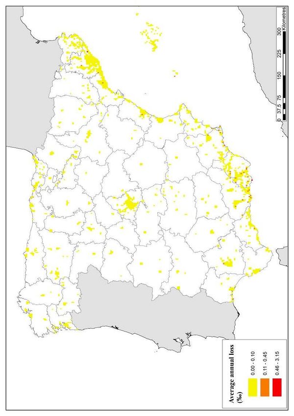
5.4.1 Comparison of the PML for different hazard models

Having mentioned the recent trend to use different Cat-Models in order to compare, validate and even produce final results (Calder et al., 2012), in this section a comparison of risk results, in terms of the PML plot is presented by using two different hazard models. The first results, denoted as Model 1 are the same as in Figure 5.3 where the seismic hazard model explained in this study has been used, while the second one, denoted as Model 2 correspond to the hazard model calculated using a smoothed seismicity approach (Ordaz et al., 2014b). In both cases the exposure database and vulnerability functions are the same. Figure 5.5 shows the results from where it can be seen that, as expected, the risk results are not exactly the same, both models lead to the same order of magnitude.

Figure 5.5. Comparison of earthquake PML for the urban areas of Spain using different seismic hazard models

In case a decision is to be made to develop any of the applications that fit onto a comprehensive disaster risk management scheme, the decision-maker when faced to the details of both hazard models, if they are transparent as the example presented here, may judge and select the most appropriate one for the case.

5.5 PROBABILISTIC SEISMIC RISK ASSESSMENT RESULTS AT
LOCAL LEVEL FOR LORCA

A fully probabilistic seismic risk assessment has been performed for Lorca, a city belonging to the Murcia region. The selection of a higher resolution level for the analysis allows considering more details including the evaluation of the seismic hazard by for example considering the local site-effects. Anyhow, even if using the same arithmetic as in the previous example, it is noteworthy to realize that modifying the scale of the exposure database may imply an abrupt change in scope and resources associated to the risk assessment, especially in countries/regions where there is little information.

Two different probabilistic seismic risk assessments were performed in Lorca. In the first stage, a single scenario analysis was conducted using a scenario with similar characteristics to the one that which occurred in May 2011. Results of the modelling were obtained in terms of MDR and the aggregated loss values and damage levels were compared with the official post-earthquake survey conducted by the local officials. On the other hand, a fully probabilistic seismic risk assessment, considering all the earthquake scenarios included in the stochastic set was performed and risk results were obtained in terms of the LEC from where other metrics such as the AAL and PML were obtained.

5.5.1 Results for the single scenario

Even if the recorded damages after earthquakes are limited, there have been different attempts to compare predicted vulnerability and damage levels with those observed after post-event damage surveys for specific building classes and different resolution levels (Benedetti and Benzoni, 1985; Crowley et al., 2008). Also, a model for reproducing a damage scenario for Lorca was developed using fragility curves (Rivas-Medina et al., 2014) and a fully probabilistic risk assessment for the Murcia region was performed after the earthquake by Valcárcel et al. (2012). All of them have concluded that although not matching the modeled and the observed figures in an exact way, said comparisons have allowed identifying that Cat-Models are useful for the estimation of order of magnitudes of potential losses keeping in mind the limitation that many parameters considered as objective are in reality subjective and depend significantly on expert judgment. Also, in all the above mentioned cases, what have been compared are the damages and not the losses.

On May 11^th at 18:47 a shallow 5.1 (Mw) earthquake occurred with epicenter located 5 km away from Lorca causing several damages in buildings located in the Murcia Region, being that the most affected city both in terms of structural damage, disruption and casualties. From the set of stochastic scenarios and knowing the characteristics in terms of magnitude, location and depth of the real event, a scenario with similar characteristics was identified and selected for the analysis. Figure 5.6 shows the PGA for the selected scenario while Table 5.2 summarizes some of the main parameters.

At this stage is important to say that the comparison of a single event (and the associated seismic intensities) against the integrated seismic hazard results for any region cannot be performed. Whilst the first represent the results of a unique event, the second approach, as explained in the PSHA section considers the participation of several events that have different magnitudes, different locations and can even be associated to different seismogenetic sources. What, for example, can be done after an event occurred is to validate, using an appropriate GMPE, that the associated seismic intensity correspond, in order of magnitudes to the M-R pair and also that its location is within the geometrical possibilities of the modelled seismogenetic sources (Iervolino, 2013), a procedure that has been conducted for this particular event and complies in all aspects.

Figure 5.6. Shakemap (PGA) for the selected event (cm/s²)

Table 5.2. Scenario characteristics

The vulnerability functions presented in the previous section were used and the convolution process between them and the hazard scenario was performed. For that scenario, around €615 million were obtained which correspond to 8.9% of the total exposed value. Again, it is worth noting that this value only considers the direct physical damage and other aspects such as the historical, heritage and cultural values of the elements are not included and are out of the scope of this study.

Besides obtaining a gross value of the expected losses, this analysis allows disagregating the results in several categories (as much as the ones included in the exposure database). For example, Table 5.3 shows the expected losses classified by building class from where it can be observed that most of the losses are concentrated mainly in masonry and earthen structures.

Table 5.3. Expected damage and MDR by building class

Additionally, results can be also disaggregated by construction date as presented in Table 5.4. From those results it can be concluded that, as expected, older buildings that are more vulnerable because poor maintenance and having lower specifications in the used building codes at the time of design and construction, concentrate higher expected losses.

Table 5.4. Expected damage and MDR by construction date

Again, this loss values in monetary units correspond to those associated to direct physical damage when then, issues like price increase in handwork and construction materials because of multiple damages within the same region (known as damage surge) cannot be captured. They also largely depend on specific local production conditions and are not feasible to be included within the selected approach for this study.

Since the risk assessment has been performed on a geo-referenced database, it is possible to obtain the geographical distribution of the expected losses and damages in terms of monetary units or also MDR for the exposed assets in Lorca. Figure 5.7 shows the expected loss geographical distribution by dwelling in Lorca. Although it contains relevant information associated to the damage and loss levels in each element, it does not explicitly show which elements have the highest risk. For example, a loss of €10,000 can correspond to a 1% MDR of an element which appraisal is equal to €1 million, while a loss of €4,000 at the same time can correspond to a 45% MDR of an element appraised in €10,000. Erroneously, one may think that the building with the highest associated loss may have a higher risk.

Because of that, risk results, when presented through maps, are better understood if the risk results are normalized by their exposed value. In that case it means that the best metric to select is the MDR as shown in Figure 5.8 where for example it can be clearly seen that the highest damage levels are concentrated in the historical centre of the city as well as in the zones with the oldest (and more vulnerable) structures.

Figure 5.7. Expected loss for the modelled scenario in Lorca

Figure 5.8. MDR (%) for the modelled scenario in Lorca

5.5.2 Comparison with the damage levels recorded after May’s 2011 earthquake

The May 2011 earthquake that stroke Lorca, associated to the Alhama de Murcia fault which extends for more than 100 km, that also has an inverse focal mechanism, although having a moderate magnitude caused several casualties (9 death and more than 300 injured) and important structural damage that did not allow more than 10,000 people to return to their homes. Also, two health centers were evacuated because of severe structural damage that threatened both patients and medical personnel. The earthquake led to a chaotic situation in the post-earthquake phase because no previous experience in the implementation of an emergency plan existed, notwithstanding the delay in many of the response actions (Barbat et al., 2011a).

According to the damage survey conducted by the local administration (Ayuntamiento de Lorca), 19% of the buildings were not inspected since, at first sight, they only suffered minor damage. 52% of the inspected buildings were classified as habitable because of the lack of important damage, 16% of the inspected buildings were classified with restricted access since no structural damage occurred but non-structural elements were affected, 9% of the inspected buildings were classified with prohibited access because high structural damage levels and finally, for 4% of the inspected buildings a demolition order was issued (Ayuntamiento de Lorca, 2012).

Insured losses, mostly related to residential and commercial units reached almost €490 million (CCS, 2012) and, although that figure does not correspond to the direct damage cost in Lorca, since not all underwritten insurance policies have the same conditions and there are particular deductible and limit conditions on each of them, can be used as a reference order of magnitude value.

Regarding the characteristics of the observed damage it can be said that many shear stress damages were observed in masonry units that, as seen in the exposure section, constitute a vast majority of the building stock in Lorca. For reinforced concrete dwellings, damage associated to facades and division walls (mainly built with brick masonry) was commonly observed but also, in waffled-slab buildings, damage associated to shear stresses was observed. Finally, damages because of the short column typology was observed in the reinforced concrete dwellings and even more, the only building that collapsed during the earthquake failed because of that effect.

This section presents a comparison between the observed and recorded damage after the earthquake according to the official post-event damage survey and the modeled scenario whose results were previously shown. According to the damage survey performed by the Ayuntamiento de Lorca (2012), affected elements were classified in the next four categories:

1. Habitable (green)

2. Restricted access because damage on non-structural elements (yellow)

3. Prohibited access because structural damage requiring repairing and retrofitting measures (red).

4. Mandatory demolition order (black)

A total of 7,852 buildings were inspected, accounting for approximately 44% of the buildings in Lorca. It was observed that 19% of those did not suffer any significant damage. The distribution of recorded damage among the four categories is shown in Table 5.5.

Table 5.5. Recorded damage statistics and categories for the Lorca earthquake

These results have the same order of magnitude than other damage surveys conducted in the city by other experts and institutions (Benito et al. 2012; IGN et al. 2011, Barbat et al. 2011b, Álvarez et al. 2013; Menéndez et al. 2012).

The damage survey was geo-located and the damage map shown in Figure 5.9 is available online (Ayuntamiento de Lorca 2012). The number of inspected buildings can be considered as statistically significant and then useful for establishing damage distributions along Lorca.

Figure 5.9. Online damage viewer with the recorded damage levels

In order to compare the observed with the simulated damage, MDR ranges were set to represent the different damage categories. It is assumed that buildings need a demolition order if MDR is higher than 40%; have forbidden access if MDR is between 16 and 39.9%; have restricted access if MDR is between 10 and 15.9%; are habitable if MDR is between 4 and 9.9%; and have no damage if MDR is lower than 4%. According to these levels, the statistics for all buildings in Lorca is presented in Table 5.6.

Table 5.6. Modelled damage categories for the scenario in Lorca

The percentage values of the simulated scenario are similar in all damage categories presented in Table 5.5 with the exception of the buildings with demolition order. Figure 5.10 shows the simulated results grouped in damage categories.

Figure 5.10. Damage categories geographical distribution for the modelled scenario in Lorca

As it is well known, physical risk estimations are intended to provide an order of magnitude of the expected losses and their average frequency of occurrence if a loss exceedance curve is computed, and not to predict the exact damage and its geographical location in the area under analysis.

A model calibration is not possible from a methodological point of view because it cannot be based on a unique observed damage case. Even more, the coincidence of the modelled results with a single observation can even be interpreted as a mere coincidence. Even if Cat-Models are only providing estimations of the feasible future losses, the statement made by the British philosopher Carveth Read that “It is better to be vaguely right than exactly wrong” applies.

After a disaster occurs, performing a good quantification of the losses is not an easy task and big challenges arise when trying to disaggregate the records by categories. Double counting and the aggregation level have to do with the final recorded values (Cochrane, 2004). Also in Lorca, defining that no damage (and loss) occurred by a single and simple observation may not be sufficient for a rigorous comparison.

Since Cat-Models are mostly intended to work on a global basis, a single event is clearly not statistically significant. Moreover, catastrophic events have low occurrence frequencies and thus there are no sufficient observed damage and loss records available which can be used in a comprehensive calibration process. Obviously, even if a Cat-Model is adjusted to match the observed damage for a unique event, this does not guarantee the reliability for a different event at a different location with different characteristics. On the other hand, no amount of observations can deny the possibility of a surprise (Woo, 2011).

Catastrophe events have associated a power law and because of that, errors even two-folding what is being modelled and observed (or the other way round) can be considered as acceptable (Woo, 2011). Again, the main objective of the Cat-Models is not to exactly predict what is going to happen in the future but to provide an order of magnitude of the expected losses.

Also, as a reflection of what happened in Lorca after the earthquake, it is important to mention that many buildings were not demolished because they presented a high level of damage and could not be retrofitted or repaired but due to social, institutional and insurance reasons. Also, it is important to remember that a catastrophic event, by destroying the most vulnerable elements, can somehow decrease the risk level whilst also the reconstruction process can represent an economic boost for the affected region and in the medium-long term lead to improvements in the economic performance from a macroeconomic perspective.

Even if today there are still many structures to be rebuilt in Lorca, the reconstruction process has assured the use of the updated earthquake resistant building code where it is expected that the overall vulnerability of the building stock is to decrease. Since a considerable number of elements were given a mandatory demolishing order, if a future assessment considering the new (and in theory lower) vulnerability levels, it should provide lower loss values than the presented in this study.

5.5.3 Comprehensive and fully probabilistic seismic risk results for Lorca

The second stage of the probabilistic seismic risk assessment in Lorca consists in a fully probabilistic assessment where now not only one but more than 50,000 scenarios are considered for the evaluation. The methodology is the same as the presented for the national risk assessment and the seismic hazard model corresponds to the presented in this document while the exposure database and vulnerability functions are the same as for the scenario analysis presented before.

Because a complete set of stochastic scenarios was considered, it is possible to express the risk results for Lorca in terms of the LEC as shown in Figure 5.11 (Salgado-Gálvez et al., 2015b). In this case, a log-log scale has been selected for both axis and it is the reason for the difference in the shape if compared to the national level LEC presented in Figure 5.1.

Figure 5.11. Earthquake Loss Exceedance Curve for Lorca

Table 5.7 shows a summary of the risk results in terms of the AAL and selected PML and now, relative risk values are much higher that a national level. A 2.4‰ relative AAL combined with relative PMLs close to 10% of the total exposed value, represent a high risk level.

Table 5.7. Summary of seismic risk results for Lorca

Figure 5.12 shows the PML plot for Lorca that, as explained before, contains exactly the same information as the LEC but arranged in a different style.

Figure 5.12. Earthquake PML plot for Lorca

Seismic risk results can be disaggregated according to the categories included in the exposure database so that they can be useful not only to have an idea of the geographical concentration of the risk but to know which building classes, age ranges and heights, have the highest risk. In all cases, the chosen risk metric to present the results is AAL (both absolute and relative) because of the advantages presented at the beginning of this section.

Table 5.8 shows the seismic risk results disaggregation by building class for Lorca, from where it can be seen that the building class with highest relative AAL is the earthen one, followed by masonry (brick and stone dwellings). An important finding here corresponds to the masonry walls and R/C buildings that it is well-known to have poor performance under earthquake loads and, therefore, a high relative AAL.

Table 5.8. Probabilistic seismic risk results disaggregation by building class in Lorca

Table 5.9 shows the results disaggregation by age range from where it can be seen that the relative AAL increase with the age of the structure. One of the parameters not captured in this assessment is if the dwelling had any retrofitting measure between the construction time and the cadastral database assembly process and it is assumed that nothing occurred.

Table 5.9. Probabilistic seismic risk results disaggregation by age range in Lorca

Finally, Table 5.10 shows the results disaggregation by height range from where first it can be seen that the building stock of Lorca is mostly comprised by low rise structures (between 1 and 3 stories) and of course most of the absolute AAL figures are concentrated there. On the other hand, considerable lower relative AAL exist between the different height ranges that can be explained by the use of strict standards and earthquake resisting building codes when structures of said size are built.

Table 5.10. Probabilistic seismic risk results disaggregation by height range in Lorca

As in the case of the single scenario assessment, seismic risk maps can be obtained for the fully probabilistic case. The best metric to represent seismic risk in graphical terms is the AAL either in absolute (Figure 5.13) or in relative (Figure 5.14) terms. In absolute terms, the same problem as the absolute MDR can arise and there may be cases where the highest values may correspond to the most expensive buildings and not the ones with actually the highest risk. Because of that, normalized AAL is preferred for seismic risk representation through maps.

Figure 5.13. Average Annual Loss (absolute) for the building stock in Lorca

Figure 5.14. Average Annual Loss (relative) for the building stock in Lorca

When reliable information about the total constructed area is available, such as it is the case for Lorca, an interesting combination between risk results and it can be obtained. In this case, the absolute AAL has been divided by the total constructed area of the dwellings and the geographical distribution of it is shown in Figure 5.15.

Figure 5.15. Absolute Average Annual Loss per constructed square meter in Lorca

Given that earthquakes associated to different seismogenetic sources can cause damages and losses in Lorca and, also, since an event-based approach has been selected for the risk assessment, it is possible to disaggregate the AAL by seismogenetic source to see the overall contribution of the events associated to them in the total value. Figure 5.16 presents those results from where it can be seen that most of the events contributing to the AAL are associated to the ESAS250 source with a participation above 88%, whilst events associated to the Africa, ESAS 246 and ESAS247 seismogenetic sources account for approximately 10% of the AAL.

Figure 5.16. Relative AAL participation by seismogenetic source

The reason for the big difference between the national and local relative seismic risk levels lies mainly on the geographical distribution of the exposed assets. Whilst in the first case, elements are distributed along the Peninsula and Balearic Islands but not all of them are exposed to earthquakes, in the second case, all dwellings in Lorca are located in seismic hazard prone areas.

In the case that specific risk transfer mechanisms were to be developed for any of the two case studies, the approaches for them must be different. In the first case, because of the geographical distribution of the exposed elements lower loss correlation is to be expected since, even if a strong earthquake occurs, the number of damaged assets, relative to the total, if compared with the local assessment. In some cases catastrophic losses are insured at national level using the same premium value for all elements, an issue that whilst having an advantage from a solidarity perspective, may generate incentives about using high hazard prone areas and poor construction practices.

5.6 USING THE PROBABILISTIC SEISMIC RISK RESULTS AT URBAN LEVEL

Quantifying seismic risk is not an ending point but a starting point in a comprehensive risk management scheme. As explained in the foreword, this key stage allows identifying, in many cases, where risk is concentrated and therefore, helps planning specific actions in order to mitigate it. Not all the measures that can be taken are related to structural retrofitting actions and in some cases, financial arrangements in order to guarantee access to the required funds in an expedite way after a disaster occurs can be based on results like the ones obtained for Lorca. By having taken ex-ante measures related to the financial planning of the required resources, does not only guarantees the availability of said resources to be used on time, but decreases the transaction and negotiation costs since obtaining loans and credits after a disaster, may lead to higher interest rates and less favorable payment conditions. Collective urban catastrophe insurance schemes, such as the one successfully implemented in Manizales, Colombia (Marulanda et al., 2014) can be based on robust models such as the one presented here.

Because risk has several dimensions, the physical results can be integrated into comprehensive and holistic approaches to obtain an urban seismic risk index (USRi) (Cardona, 2001; Carreño, 2006; Carreño et al., 2007; 2012) where a set of factors related to social fragility and lack of resilience aggravate the physical risk conditions. Results are usually calculated for different zones of the urban areas such as neighborhoods or administrative divisions allowing direct comparison among them. Since several factors are combined in this approach and those can be capturing very different aspects of a society (i.e. available public area, delinquency rates), the final USRi value can be disaggregated and therefore identify which of the factors is most contributing to it. The results obtained in this study can be used as input in the EvHo tool (CIMNE-RAG, 2014) to calculate the USRi using both a probabilistic and holistic approach.

Since the CAPRA Platform (see Annex G) allows calculating risk with a multi-hazard approach, the results obtained in this study can be combined with for example landslide susceptibility analysis using the methodology proposed by Ordaz (2014) in Lorca. As it is known, several landslides occurred because of the May 2011 earthquake along the Murcia Region and it is a field of further research that can be comprehensively integrated with the results obtained in this study.

REFERENCES

Abrahamson N.A. (1988). Statistical properties of peak ground accelerations recorded by the SMART 1 array. Bulletin of the Seismological Society of America. 78(1):26-41.

Abrahamson N.A. (2000). Prestandard and commentary for the seismic rehabilitation of buildings. Federal Emergency Management Agency. FEMA-356 report.

Agnanos T. and Kiremidjian A.S. (1988). A review of earthquake occurrence models for seismic hazard analysis. Probabilistic Engineering Mechanics. 3(1):3-11.

AIS – Asociación Colombiana de Ingeniería Sísmica (2013). Recomendaciones para requisitos sísmicos de estructuras diferentes de edificaciones. Bogotá, Colombia.

AIS – Asociación Colombiana de Ingeniería Sísmica (2010). Reglamento Colombiano de Construcción Sismo Resistente. Bogotá, Colombia.

Albala-Bertrand J.M. (2006). The unlikeliness of an economic catastrophe: localization and globalization. Queen Mary University of London. Department of Economics. London, U.K.

Albala-Bertrand J.M. (1993). Natural disaster situations and growth: A macroeconomic model for sudden disaster impacts. 21(9):1417-1434.

Álvarez R., Díaz-Pavón E., Rodríguez R. (2013). El terremoto de Lorca, efectos en los edificios. Consorcio de Compensación de Seguros.

Ambraseys N., Douglas J., Sarma K. and Smit P. (2005). Equations for the estimation of strong ground motions from shallow crustal earthquakes using data from Europe and the Middle East: Horizontal peak ground acceleration and spectral acceleration. Bulletin of Earthquake Engineering. 3(1). 1-53.

Andersen T.J. (2002). Innovative financial instruments for natural disaster risk management. Technical paper, Inter-American Development Bank.

ATC – Applied Technology Council (1996). ATC-40. Seismic evaluation and retrofit of concrete buildings. California, USA.

ATC – Applied Technology Council (1985). ATC-13. Earthquake damage evaluation data for probable maximum loss studies of California buildings. California, USA.

Arrow K.J. (1996). The theory of risk-bearing: small and great risks. Journal of risk and uncertainty. 12:103-111.

Arrow K.J. and Lind R.C. (1970). Uncertainty and the evaluation of public investment decisions. The American Economic Review. 60(3):364-378.

Arroyo D., Ordaz M. and Rueda R. (2014). On the selection of Ground-Motion Prediction Equations for Probabilistic Seismic-Hazard Analysis. Bulletin of the Seismological Society of America. 104(4):1860-1875.

Ayuntamiento de Lorca. (2012). “Visor geográfico seismo de Lorca del 11 de mayo de 2011”, http://www.lorca.es/seismo11demayo/seismo11demayo.asp?id=1540. Accessed on January 03, 2014.

Baker J.W. and Cornell C.A: (2006). Which spectral acceleration are you using? Earthquake Spectra. 22(2):293-312.

Banks E. (2004). Alternative risk transfer: integrated risk management through insurance, reinsurance and the capital markets. Wiley Finance. 238pp.

Barbat A.H. (1998). El riesgo sísmico en el diseño de edificios. Calidad Siderúrgica. Madrid.

Barbat A.H., Carreño M.L., Figueras S., Goula X., Irizarry J., Lantada N., Macau A. and Valcárcel J. (2011a). El terremoto de Lorca del 11 de mayo de 2011. Institut Geològic de Catalunya-IGC. Barcelona.

Barbat A. H., Carreño M.L., Cardona O.D. and Marulanda M. (2011b). Evaluación holística del riesgo sísmico en zonas urbanas. Revista Internacional de Métodos Numéricos para Cálculo y Diseño en Ingeniería. 27(1):3-27.

Barbat A. H., Lagomarsino S. and Pujades L. (2006). Vulnerability assessment of dwelling buildings. In: Assessing and managing earthquake risk. C Sousa, X Goula and A. Roca editors. 115-134. Springer

Barbat A. H., Mena U., and Yépez F. (1998). Evaluación probabilista del riesgo sísmico en zonas urbanas. Revista Internacional de Métodos Numéricos para Cálculo y Diseño en Ingeniería. 14(2):247-268.

Barbat A. H. and Bozzo L. (1997). Seismic analysis of base isolated buildings. Archives of Computational Methods in Engineering. 4(2):153-192.

Bazzurro, P. and Luco, N. (2005). Accounting for uncertainty and correlation in Earthquake loss estimation. ICOSSAR. 2687-2694.

Bender B. (1983). Maximum likelihood estimation of b values for magnitude grouped data. Bulletin of the Seismological Society of America. 73(3):831-851.

Bender B. and Perkins D.M. (1987). SEISRISK III: A computer program for seismic hazard estimation. United States Geological Survey – USGS. Bulletin 1772. 48pp.

Benedetti D. and Benzoni G.M. (1985). Seismic vulnerability index vs damage for unreinforced masonry buildings. US-Italy workshop on seismic hazard and risk analysis.

Benito B., Rivas A., Gaspar-Escribano J. and Murphy P. (2012). El terremoto de Lorca (2011) en el contexto de la peligrosidad y el riesgo sísmico en Murcia. Física de la Tierra. 24:255-287.

Benito B. and Gaspar-Escribano J.M. (2007). Ground motion characterization and seismic hazard assessment in Spain: context, problems and recent developments. Journal of Seismology. 11. 433-452.

Benito B., Carreño E., Jiménez M., Murphy P., Martínez J., Tsige M., Gaspar-Escribano J. García M., García J., Canora C., Álvarez J and García I. (2005). Riesgo Sísmico en la Región de Murcia – RISMUR. Instituto Geográfico Nacional. Spain.

Bernal G.A. (2014). Metodología para la modelación, cálculo y calibración de parámetros de la amenaza sísmica para la evaluación probabilista del riesgo. Ph.D. Thesis. Polytechnic University of Catalonia. Barcelona, Spain.

Birkmann J. (ed.) (2014). Measuring vulnerability to natural hazards: towards disaster resilient societies. Second edition. United Nations University Press.

BMZ – Federal Ministry for Economic Cooperation and Development (2014). The vulnerability sourcebook. Concept and guidelines for standardized vulnerability assessments.

Bohn J.G. and Hall B. (1999). The moral hazard of insuring the insurers. In: The financing of Catastrophe Risk. Froot K.A. (ed). National Bureau of Economic Research. Universtiy of Chicago Press.

Bommer J.J. (2012). Challenges of building logic trees for probabilistic seismic hazard analysis. Earthquake Spectra. 28(4):1723-1735.

Bommer J.J. and Crowley H. (2006). The influence of ground-motion variability in earthquake loss modelling. Bulletin of Earthquake Engineering. 4:231-248.

Boore D. (1983). Stochastic simulation of high-frequency ground motion based on seismological models of radiated spectra. Bulletin of the Seismological Society of America. 73. 1865-1884.

Bozzo L. and Barbat A. (2000). Diseño sísmico de edificios, técnicas convencionales y avanzadas. Editorial Reverté S.A. Barcelona, Spain.

Brune J. (1970). Tectonic stress and the spectra of seismic S waves from earth. Journal of Geophysical Research. 75. 4997-5009.

Buforn E., Bezzeghoud M., Udías A. and Pro C. (2004). Seismic Sources on the Iberia-African Plate Boundary and their Tectonic Implications. Pure and Applied Geophysics. 161. 623-646.

Buforn E. and Udías A. (2007). Sismicidad y mecanismo focal de los terremotos de la región Cabo de San Vicente-Argelia. Revista de la Sociedad Geológica de España. 20(3-4). 301-310.

Buforn E., Udías A. and Colombás M.A. (1988). Seismicity, source mechanisms and seismotectonic of the Azores-Gibraltar plate boundary. Tectonophysics. 11. 111-137.

Caers J. (2011). Modeling Uncertainty in the Earth Sciences. Wiley-Blackwell.

Calder A., Couper A. and Lo J. (2012). Catastrophe model blending techniques and governance. The actuarial profession.

Cardona O.D. (2009). La gestión financiera del riesgo de desastre. Instrumentos financieros de retención y transferencia para la Comunidad Andina. PREDECAN. Lima, Perú.

Cardona O.D. (2001). Estimación holística del riesgo sísmico utilizando sistemas dinámicos complejos. Ph.D. Thesis. Polytechnic University of Catalonia. Barcelona, Spain.

Cardona O.D., Ordaz M.G., Mora M., Salgado-Gálvez M.A., Bernal G.A., Zuloaga-Romero D., Marulanda M.C., Yamín L. and González D. (2014). Global risk assessment: a fully probabilistic seismic and tropical cyclone wind risk assessment. International Journal of Disaster Risk Reduction. 10:461-476.

Cardona O.D., Ordaz M., Reinoso E., Yamín L.E. and Barbat A.H. (2012). CAPRA – Comprehensive Approach to Probabilistic Risk Assessment: International Initiative for Risk Management Effectiveness. Proceedings of the 15^th World Conference on Earthquake Engineering. Lisbon, Portugal.

Cardona O.D., Ordaz M., Reinoso E., Yamín L.E. and Barbat A. (2010). Comprehensive Approach to Probabilistic Risk Assessment (CAPRA); International initiative for disaster risk management effectiveness. Proceedings of the 14^th European conference on earthquake engineering, Ohrid, Macedonia.

Cardona O.D., Ordaz M., Yamín L.E., Marulanda M.C. and Barbat A.H. (2008a). Earthquake loss assessment for integrated disaster risk management. Journal of Earthquake Engineering. 12(S2):48-59.

Cardona O.D., Ordaz M., Marulanda M.C. and Barbat A.H. (2008b). Estimation of probabilistic seismic losses and the public economic resilience – An approach for macroeconomic impact evaluation. Journal of Earthquake Engineering. 12(S2):60-70.

Carreño M.L. (2006). Técnicas innovadoras para la evaluación del riesgo sísmico y su gestión en centros urbanos: Acciones ex ante y ex post. Doctoral Thesis. Universidad Politécnica de Cataluña, Barcelona, Spain.

Carreño M.L., Cardona O.D. and Barbat A.H. (2012). New methodology for urban seismic risk assessment from a holistic perspective. Bull. of earthq. eng. 10(2): 547-565.

Carreño M.L., Cardona O.D. and Barbat A.H. (2007). Urban seismic risk evaluation: a holistic approach. Nat. Hazards. 40(1): 137-172.

Carreño M.L., Cardona O.D. and Barbat A.H. (2005). Sistema de indicadores para la evaluación de riesgos. Monografía de Ingeniería Sísmica IS-52. ISBN: 84-95999-70-6. Centro Internacional de Métodos Numéricos en Ingeniería. Barcelona, Spain.

Carreño M.L., Cardona O.D. and Barbat A.H. (2004). Metodología para la evaluación del desempeño de la gestión del riesgo. Monografía de Ingeniería Sísmica IS-51. ISBN: 84-95999-66-8. Centro Internacional de Métodos Numéricos en Ingeniería. Barcelona, Spain.

Chávez-López G. and Zolfaghari M. (2010). Natural catastrophe loss modelling: the value of knowing how little you know. Proceedings of the 14^th European Conference on Earthquake Engineering. Ohrid, Macedonia.

CIMNE, ITEC, INGENIAR and EAI (2013). Probabilistic modelling of natural risks at the global level: Global Risk Model. Background paper for the Global Assessment Report on Disaster Risk Reduction 2013.

CIMNE-RAG (2014). Holistic risk evaluation tool EvHo V1.0. Program for computing holistic risk at urban level. Centro Internacional de Métodos Numéricos en Ingeniería, CIMNE, Risk Assessment Group, RAG, Barcelona, Spain.

Coburn A. and Spence R. (2002). Earthquake protection second edition. Wiley 436pp.

Cochrane H. (2004). Economic loss: myth and measurement. Disaster prevention and management. 13(4):290-296.

Cornell, C. A., and E. H. Van Marke (1969). The major influences on seismic risk, in Proceedings of the Third World Conference on Earthquake Engineering, Santiago, Chile, A-1, 69–93.

Crowley H., Stafford P.J. and Bommer J.J. (2008). Can earthquake loss models be validated using field observations? Journal of Earthquake Engineering. 12:1078-1104.

Crowley H. and Bommer J.J. (2006). Modelling seismic hazard in earthquake loss models with spatially distributed exposure. Bulletin of Earthquake Engineering. 4:249-273.

De Bono A. and Mora M.G. (2014). A global exposure modelfor disaster risk assessment. International Journal of Disaster Risk Reduction. 10:442-451.

De Vicente G., Cloetingh S., Muñoz A., Olaiz A., Stich D., Vegas R., Galindo J. and Fernández J. (2008). Inversion of moment tensor focal mechanisms for active stresses around the microcontinent Iberia: Tectonic implications. Tectonics. 27. 1-22.

De Vicente G., Vegas R., Guimera J., Muñoz A., Casas A., Martín S., Heredia N., Rodríguez L. González J. Cloetingh S., Andeweg B., Álvarez J. and Olaiz A. (2004). Evolución geodinámica cenozoica de la placa ibérica y su registro en el antepaís. Geología de España. 597-602. SGE.IGME, Madrid, Spain.

Der Kiureghian and Ditlevsen O. (2009). Aleatory or epistemic? Does it matter? Structural safety. 31:105-112.

Douglas R. (2014). Integrating natural disaster risks and resilience into the financial system. Willis Research Network. Concept Note. London, U.K.

Egozcue J., Barbat A., Canas J., Miquel J. and Banda E. (1991). A method to estimate occurrence probabilities in low seismic activity regions. Earthquake Engineering and Structural Dynamics. 20(1):43-60.

ERN-AL Consortium (2011). ERN-Vulnerabilidad. Program for developing vulnerability functions. http://www.ecapra.org

ERN-AL Consortium (2009). Perfil de riesgo catastrófico por terremoto y huracán. Informe Técnico ERN-CAPRA-T3-5.

Esteva L. (1967). Criterios para la construcción de espectros de diseño sísmico. Proceedings of the third Pan-American Symposium of Structures. Caracas, Venezuela.

ECS – European Committee for Standardisation (2004). Eurocode-8: Design of structures for earthquake resistance.

FEMA – Federal Emergency Management Agency (2011). Multi-hazard loss estimation methodology. Earthquake Model HAZUS-MH 2.1 Technical Manual.

FEMA – Federal Emergency Management Agency (1997). FEMA-273. NEHRP guidelines for the seismic rehabilitation of buildings.

Field E.H., Jordan T.H. and Cornell C.A. (2003). OpenSHA: A developing community-modeling environment for seismic hazard analysis. Seismological Research Letters. 74:406-419.

Fischhoff B. (1994). Acceptable risk: a conceptual proposal. Available at: http://www.piercelaw.edu/risk/vol5/winter/fischhof.htm

Freeman P., Keen M. and Mani M. (2003). Dealing with increased risk of natural disasters: challenges and options. Vol N.8 2003-2197. International Monetary Fund. Fiscal Affairs Department.

García L.E. (1998). Dinámica estructural aplicada al diseño sísmico. Universidad de Los Andes. Bogotá, Colombia.

García-Mayordomo J. (2005). Caracterización y análisis de la peligrosidad sísmica en el sureste de España. Ph.D. Thesis. Universidad Complutense de Madrid. Madrid, Spain.

García-Mayordomo J., Gaspar-Escribano J.M. and Benito B. (2007). Seismic hazard assessment of the Province of Murcia (SE Spain): analysis of source contribution to hazard. Journal of Seismology. 11. 453-471.

Gardner J.K. and Knopoff L. (1974). Is the sequence of earthquakes in Southern California with aftershocks removed, Poissonian? Bulletin of the Seismological Society of America. 64. 1363-1367.

GRCG – German Research Center for Geosciences. (2010). Seismic Hazard Harmonization in Europe SHARE. Development of a common methodology and tools to evaluate earthquake hazard in Europe. Theme 6: Environment. German Research Center for Geosciences.

GFDRR – Global Facility for Disaster Reduction and Recovery (2014a). Understanding Risk. Review of Open Source and Open Access Software Packages Available to Quantify Risk from Natural Hazards. Washington D.C., USA.

GFDRR – Global Facility for Disaster Reduction and Recovery (2014b). Understanding Risk. The evolution of disaster risk assessment. Washington D.C., USA.

Gini C. (1912). Variabilita e Mutuabilita. Contributo allo Studio delle Distribuzioni e delle Relazioni Statistiche. C. Cuppini. Bologna, Italy.

Global Reinsurance (2013). Opening the black box. Special report: CAT Modelling.

Grossi P. (2000). Quantifying the uncertainty in seismic risk and loss estimation. Proceedings of the Second EuroConference on global change and catastrophe risk management: Earthquake risks in Europe.

Grossi P., Kleindorfer P. and Kunreuther H. (1998). The impact of uncertainty in managing seismic risk: the case of earthquake frequency and structural vulnerability. The Wharton School, University of Pennsylvania.

Grünthal G. (1998). European Macroseismic Scale. Centre Européen de Géodynamique et de Séismologie.

Grünthal G., Bosse C., Sellami S., Mayer-Rosa D. and Giardini D. (1999). Compilation of the GSHAP regional seismic hazard for Europe, Africa and the Middle East. Annali di Geofisica. 42(6). 1215-1223.

Gurenko E.N. (2004). Catastrophe risk and reinsurance. ISBN: 9781906348823

Gutenberg R. and Richter C. (1944). Frequency of earthquakes in California. Bulletin of the Seismological Society of America. 34. 185-188.

Guy Carpenter (2011). Managing catastrophe model uncertainty. Issues and Challenges.

Hallegate S. and Przyluski V. (2010). The economics of natural disasters. Concepts and methods. The World Bank. Policy Research Working Paper 5507.

Hochrainer S., Timonina A., Williges K, Pflug G and Mechler R. (2013). Modelling the economic and fiscal risks from natural disasters. Insights based on the CatSim model. Background paper prepared for the Global Assessment Report on Disaster Risk Reduction 2013.

Iervolino I. (2013). Probabilities and fallacies: why hazard maps cannot be validated by individual earthquakes. 29(3):1125-1136.

IGN - Instituto Geográfico Nacional and UPM - Universidad Politécnica de Madrid. (2013a). Actualización de mapas de peligrosidad sísmica de España 2012. Madrid, Spain.

IGN - Instituto Geográfico Nacional. (2013b). Catálogo de terremotos. Recuperado de: http://www.ign.es/ign/layoutIn/sismoFormularioCatalogo.do

IGN - Instituto Geográfico Nacional, Universidad Complutense de Madrid, Universidad Politécnica de Madrid, Instituto Geológico y Minero de España, Asociación Española de Ingeniería Sísmica (2011). Informe del sismo de Lorca del 11 de mayo de 2011. Madrid, Spain.

INE - Instituto Nacional de Estadística. (2011). Censo de población y vivienda 2011. http://www.ine.es/censos2011_datos/cen11_datos_res_pob.htm

Jaiswal K. and Wald D. (2010). An empirical model for global earthquake fatality estimation. Earthquake Spectra. 26(4):1017-1037.

Jaramillo C.R. (2009). Do natural disasters have long-term effects on growth? Facultad de Economía, Universidad de Los Andes. Bogotá, Colombia.

Jiménez M.J. and García-Fernández M. (1999) Seismic hazard assessment on the Ibero-Maghreb region. Annali di Geofisica. 42(6). 1057-1065.

Jiménez M.J., Giardini D. and Grünthal G. (2001). Unified seismic hazard modelling throughout the Mediterranean Region. Bolletino di Geofisica Teorica e Applicata. 42(1-2). 3-18.

Joyner W.B. and Boore D.M. (1981). Peak horizontal acceleration and velocity from strong-motion records including records from the 1979 Imperial Valley, California, Earthquake. Bulletin of the Seismological Society of America. 71:2011-2038.

Kramer S, (1996). Geotechnical earthquake engineering. Ed. Prentice Hall. 653pp.

Keogh B. (2011). In: Eqecat’s Keogh stresses the limitations of models. Cat risks – ILS.

Kiremidjian A. S. and Anagnos T. (1984). Stochastic Slip-Predictable Model for Earthquake Occurrences. Bulletin of the Seismological Society of America, Vol.74, No.2,pp.739-755, April

Krinitzsky E.L. (2002). How to obtain earthquake ground motions for engineering design. Engineering Geology. 65:1-16.

Kunreuther H. (2002). Risk analysis and risk management in an uncertain world. Risk Analysis. 22(4):655-664.

Kunreuther H. and Kleffner A. (1992). Should earthquake mitigation measures be voluntary or required? Journal of Regulatory Economics. 4:321-333.

Lantada N., Irrizari J., Barbat A., Goula X., Roca A., Susagna T and Pujades L. (2010). Seismic hazard and risk scenarios for Barcelona, Spain, using the Risk-UE vulnerability index method. Bulletin of Earthquake Engineering. 8:201-229.

Lee R. and Kiremidjian A.S. (2007). Uncertainty and correlation for loss assessment of spatially distributed systems. Earthquake Spectra. 23(4):753-770.

Liechti D., Rüttener E. and Zbinden A. (2000). Disaggregation of annual average loss. Proceedings of the XXV European Geophysical Society General Assembly.

Marulanda M.C. (2013). Modelación probabilista de pérdidas económicas por sismo para la estimación de la vulnerabilidad fiscal del estado y la gestión financiera del riesgo soberano. Ph.D. Thesis. Polytechnic University of Catalonia. Barcelona, Spain.

Marulanda M.C., Cardona O.D., Mora M.G. and Barbat A.H. (2014). Design and implementation of a voluntary collective earthquake insurance policy to cover low-income homeowners in a developing country. Natural Hazards. doi:10.1007/s11069-014-1291-4.

Marulanda M.C., Carreño M.L., Cardona O.D., Ordaz M.G. and Barbat A.H. (2013). Probabilistic earthquake risk assessment using CAPRA: application to the city of Barcelona, Spain. Bulletin of Earthquake Engineering. 69:59-84.

Marulanda M.C., Cardona O.D. and Barbat A.H. (2010). Revealing the socioeconomic impact of small disasters in Colombia using the DesInventar database. Disasters. 34(2):552-570.

Marulanda M.C, Cardona O.D. and Barbat A.H. (2009). Robustness of the holistic seismic risk evaluation in urban centers using the USRi. Natural Hazards. 49(3):501-516.

Marulanda M.C, Cardona O.D., Ordaz M. and Barbat A. (2008). La gestión financiera del riesgo desde la perspectiva de los desastres: evaluación de la exposición fiscal del estado y alternativas de instrumentos financieros de retención y transferencia del riesgo. Monografía, CIMNE IS-61. Barcelona, Spain.

May P.J. (2001). Societal perspectives about earthquake performance: the fallacy of “acceptable risk”. Earthquake Spectra. 17(4):725-737.

Menéndez L., Díaz-Pavón E., Rodríguez R. and Álvarez R. (2012). El terremoto de Lorca. La necesidad de revisar algunos principios. Cuadernos INTEMAC. Vol 88.

McGuire R.K. (2004). Seismic hazard and risk analysis. Earthquake Engineering Research Institute. Oakland, California, USA.

McGuire R.K. (2001). Deterministic vs. probabilistic earthquake hazards and risks. Soil Dynamics and Earthquake Engineering. 21:377-384.

McGuire R.K. (1967). FRISK: A computer program for seismic risk analysis using faults as earthquake sources. United States Geological Survey –USGS. 90pp.

McGuire R. and Hanks T. (1981). The character of high frequency strong motion. Bulletin of the Seismological Society of America. 71. 2071-2095.

MF - Ministerio de Fomento. (2009). Norma de construcción sismorresistente. Parte general y edificación.

MHAP - Ministerio de Hacienda y Administración Pública. (2013). Dirección General del Catastro. http://www.catastro.meh.es/

Miranda E. (1999). Approximate seismic lateral deformation demands in multistory buildings. Journal of Structural Engineering. 417-426.

Muir-Wood R. (1993). From global seismotectonics to global seismic hazard. Annali di Geofisica. Vol. XXXVI, N. (3-4):153-168.

Münchener Rückversicherungs-Gesellschaft (2012). Natural Catastrophes 2011. NatCatSERVICE

Murphy C., Gardoni P. and Harris C.E. (2011). Classification and moral evaluation of uncertainties in engineering modeling. Science and engineering ethics. 17:553-570.

Navarro M., García-Jerez A., Alcalá F.J., Vidal F. and Enomoto T. (2014). Local site effect microzonation of Lorca town (SE Spain). Bulletin of Earthquake Engineering. 12:1933-1959.

Oller S., Luccioni B. and Barbat A.H. (1996). Un método de evaluación del daño sísmico en pórticos de hormigón armado. Revista Internacional de Métodos Numéricos para Cálculo y Diseño en Ingeniería. 12(2):215-238.

ORNL - Oak Ridge National Laboratory. (2007). LandScan global population distribution data. U.S. Department of Energy.

Ordaz M. (2014). A simple probabilistic model to combine losses arising from the simultaneous occurrence of several hazards. Natural Hazards. doi:10.1007/s11069-014-1495-7.

Ordaz M. (2008). Relaciones entre curvas de fragilidad, matrices de probabilidad y funciones de vulnerabilidad. Technical note. ERN.

Ordaz M. (2000). Metodología para la evaluación del riesgo sísmico enfocada a la gerencia de seguros por terremoto. Universidad Nacional Autónoma de México. México D.F.

Ordaz M., Martinelli F., Aguilar A., Arboleda J., Meletti C. and D’Amico V. (2014a) CRISIS 2014 V1.2, Program for computing seismic hazard. Instituto de Ingeniería, Universidad Nacional Autónoma de México.

Ordaz M., Cardona O.D., Salgado-Gálvez M.A., Bernal-Granados G.A., Singh S.K. and Zuloaga-Romero D. (2014) Probabilistic seismic hazard assessment at global level. International Journal of Disaster Risk Reduction. 10:419-427.

Ordaz M., Miranda E., Reinoso E. and Pérez-Rocha L.E. (2000). Seismic loss estimation model for Mexico City. Proceedings of the 12th World Conference on Earthquake Engineering.

Polackova H. (1999). Contingent government liabilities a hidden fiscal risk. Finance & Development. March

Rasmussen T.N. (2004). Macroeconomic implications of natural disasters in the Caribbean. International Monetary Fund Working Paper.

Renn O. (1992). Concepts of risk: A classification. In S. Krimsky and D. Golding (eds.): Social Theories of Risk.

RMS – Risk Management Solutions (2008). A guide to catastrophe modelling. The Review.

Rivas-Medina A., Martínez-Cuevas S., Quirós L.E., Gaspar-Escribano J.M. and Staller A. (2014). Models for reproducing the damage scenario of the Lorca earthquake. Bulletin of Earthquake Engineering. 12:2075-2093.

Satterthwaite D. (2006). Outside the large cities: the demographic importance of small urban centres and large villages in Africa, Asia and Latin America. IIED, London, UK.

Salgado-Gálvez M.A., Zuloaga D., Bernal G. and Cardona O.D. (2015a). Comparación de los resultados de riesgo sísmico en dos ciudades con los mismos coeficientes de diseño sismo resistente. Revista de Ingeniería. Universidad de Los Andes. In press.

Salgado-Gálvez M.A., Carreño M.L., Barbat A.H. and Cardona O.D. (2015b). Evaluación probabilista del riesgo sísmico en Lorca mediante simulaciones de escenarios. Revista Internacional de Métodos Numéricos para Cálculo y Diseño en Ingeniería. In press.

Salgado-Gálvez M.A., Zuloaga D., Bernal G., Mora M.G. and Cardona O.D. (2014a). Fully probabilistic seismic risk assessment considering local site effects for the portfolio of buildings in Medellín, Colombia. Bulletin of Earthquake Engineering. 12:671-695.

Salgado-Gálvez M.A, Zuloaga D., Velásquez C.A, Carreño M.L., Cardona O.D. and Barbat A.H. (2014b). Urban seismic risk index for Medellín, Colombia. A probabilistic and holistic approach. Proceedings of the Second European Conference on Earthquake Engineering. Istambul, Turkey.

Salgado-Gálvez M.A., Zuloaga D. and Cardona O.D. (2013). Evaluación probabilista del riesgo sísmico de Bogotá y Manizales con y sin la influencia de la Caldas Tear. Revista de Ingeniería, Universidad de Los Andes. 38:6-13.

Salgado-Gálvez M.A., Bernal G.A., Yamín L.E. and Cardona O.D. (2011). Evaluación de la amenaza sísmica de Colombia. Actualización y uso en las nuevas normas colombianas de diseño sismo resistente NSR-10. Revista de Ingeniería, Universidad de Los Andes. 32:28-37.

Silva V., Crowley H., Pagani M., Monelli D. and Pinho R. (2014). Development of the OpenQuake engine, the Global Earthquake Model’s open-source software for seismic risk assessment. Natural Hazards. 72-1409-1427.

Spector T. (1997). Ethical dilemmas and seismic design. Earthquake Spectra 13(3):489-504.

Spence R., Bommer J., Del Re D., Bird J., Aydinoglu N. and Tabuchi S. (2003). Comparing loss estimation with observed damage: A study of the 1999 Kocaeli Earthquake in Turkey. Bulletin of Earthquake Engineering. 1:83-113.

Starr C. (1969). Societal benefit versus technological risk. Science. American Association of the Advancement of Science.

Storchak D.A., Di Giacomo D., Bondár I., Engdahl E.R., Harris J., Lee W.H.K., Villaseñor A. and Bormann P. (2013). Public release of the ISC-GEM Global Instrumental Earthquake Catalogue (1900-2009).

The World Bank (2006). Where is the wealth of the nations? Measuring capital for the 21^st century. Washington D.C. USA.

Tinti S. and Mulargia F. (1985). An improved method for the analysis of the completeness of a seismic catalogue. Lettere al Nuovo Cimento. Series 2. 42(1). 21-27.

UNISDR – United Nations International Strategy for Disaster Risk Reduction. (2014). Progress and challenges in disaster risk reduction. A contribution towards the development of policy indicators for the Post-2015 Framework on Disaster Risk Reduction. Geneva, Switzerland.

UNISDR – United Nations International Strategy for Disaster Risk Reduction. (2013). Global Assessment Report on Disaster Risk Reduction. Geneva, Switzerland.

UNISDR – United Nations International Strategy for Disaster Risk Reduction. (2002). Natural disasters and sustainable development.

Valcárcel J., Bernal G.A. and Mora M.G. (2012). Lorca earthquake May 11 2011: a comparison between disaster figures and risk assessment outcomes. Proceedings of the 15^th World Conference on Earthquake Engineering. Lisbon, Portugal.

Vargas Y., Pujades L., Barbat A. and Hurtado J. (2013a). Capacity, fragility and damage in reinforced concrete buildings: a probabilistic approach. Bulletin of Earthquake Engineering. 11(6):2007-2032.

Vargas Y., Pujades L. and Barbat A. (2013b). Evaluación probabilista de la capacidad, fragilidad y daño sísmico en edificios de hormigón armado. Revista Internacional de Métodos Numéricos para Cálculo y Diseeño en Ingeniería. 29(2):63-78.

Vargas Y., Barbat A., Pujades L. and Hurtado J. (2013c). Probabilistic seismic risk evaluation of reinforced concrete buildings. Structures and buildings. Proceedings of the institution of civil engineering doi:10.1680/stub.12.00031.

Velásquez C.A:, Cardona O.D:, Mora M.G., Yamín L.E., Carreño M.L. and Barbat A.H. (2014). Hybrid loss exceedance curve (HLEC) for disaster risk assessment. Natural Hazards. 72:455-479.

Vielma J.C., Barbat A.H., and Oller S (2010). Seismic safety of low ductility structures used in Spain. Bulletin of Earthquake Engineering. 8(1):135-155.

Vielma J.C., Barbat A.H. and Oller S. (2009). Seismic performance of waffled-slab floor buildings. Structures and Buildings (Proceedings of the Institution of Civil Engineering). 162(SB3):169-182.

Vilanova S.P. and Fonseca J.F.B.D. (2007). Probabilistic seismic-hazard assessment for Portugal. Bulletin of the Seismological Society of America. 97(5). 1702-1717.

Wyss M., Tolis S., Rosset P. and Pacchiani F. (2013). Approximate model for world-wide building stock in three size categories of settlements. Background paper prepared for the Global Assessment Report on Disaster Risk Reduction 2013.

Woo G. (2011). Calculating catastrophe. Imperial College Press.

Zolfaghari M.R. (2000). Earthquake loss estimation model for southern Europe. Proceedings of the sixth international conference on seismic zonation.

Zuccaro G. (1998). Seismic vulnerability of Vesuvian villages: structural distributions and a possible scenario. Proceedings of the Reducing earthquake risk to structures and monuments in the EU Conference.

.

Annex A. Magnitude recurrence rate plots for the considered seismogenetic sources

Figure A.1. Magnitude recurrence plot for Africa seismogenetic source

Figure A.2. Magnitude recurrence plot for ESAS231 seismogenetic source

Figure A.3. Magnitude recurrence plot for ESAS232 seismogenetic source

Figure A.4. Magnitude recurrence plot for ESAS234 seismogenetic source

Figure A.5. Magnitude recurrence plot for ESAS241 seismogenetic source

Figure A.6. Magnitude recurrence plot for ESAS242 seismogenetic source

Figure A.7. Magnitude recurrence plot for ESAS243 seismogenetic source

Figure A.8. Magnitude recurrence plot for ESAS244 seismogenetic source

Figure A.9. Magnitude recurrence plot for ESAS245 seismogenetic source

Figure A.10. Magnitude recurrence plot for ESAS246 seismogenetic source

Figure A.11. Magnitude recurrence plot for ESAS247 seismogenetic source

Figure A.12. Magnitude recurrence plot for ESAS248 seismogenetic source

Figure A.13. Magnitude recurrence plot for ESAS249 seismogenetic source

Figure A.14. Magnitude recurrence plot for ESAS250 seismogenetic source

Figure A.15. Magnitude recurrence plot for ESAS251 seismogenetic source

Figure A.16. Magnitude recurrence plot for ESAS252 seismogenetic source

Figure A.17. Magnitude recurrence plot for ESAS253 seismogenetic source

Figure A.18. Magnitude recurrence plot for ESAS255 seismogenetic source

Figure A.19. Magnitude recurrence plot for ESAS262 seismogenetic source

Figure A.20. Magnitude recurrence plot for ESAS265 seismogenetic source

Figure A.21. Magnitude recurrence plot for ESAS270 seismogenetic source

Figure A.22. Magnitude recurrence plot for ESAS278 seismogenetic source

Figure A.23. Magnitude recurrence plot for ESAS465 seismogenetic source

Figure A.24. Magnitude recurrence plot for ESAS472 seismogenetic source

Figure A.25. Magnitude recurrence plot for ESAS474 seismogenetic source

Figure A.26. Magnitude recurrence plot for ESAS969 seismogenetic source

Figure A.27. Magnitude recurrence plot for ESAS971 seismogenetic source

Figure A.28. Magnitude recurrence plot for ESAS979 seismogenetic source

Figure A.29. Magnitude recurrence plot for FRAS115 seismogenetic source

Figure A.30. Magnitude recurrence plot for FRAS168 seismogenetic source

Figure A.31. Magnitude recurrence plot for FRAS466 seismogenetic source

Figure A.32. Magnitude recurrence plot for FRAS468 seismogenetic source

Figure A.33. Magnitude recurrence plot for FRAS469 seismogenetic source

Figure A.34. Magnitude recurrence plot for FRAS470 seismogenetic source

Figure A.35. Magnitude recurrence plot for FRAS471 seismogenetic source

Figure A.36. Magnitude recurrence plot for FRAS473 seismogenetic source

Figure A.37. Magnitude recurrence plot for MAAS269 seismogenetic source

Figure A.38. Magnitude recurrence plot for MAAS442 seismogenetic source

Figure A.39. Magnitude recurrence plot for MAAS444 seismogenetic source

Figure A.40. Magnitude recurrence plot for MAAS445 seismogenetic source

Figure A.41. Magnitude recurrence plot for PTAS27 seismogenetic source

Figure A.42. Magnitude recurrence plot for PTAS257 seismogenetic source

Figure A.43. Magnitude recurrence plot for PTAS258 seismogenetic source

Figure A.44. Magnitude recurrence plot for PTAS259 seismogenetic source

Figure A.45. Magnitude recurrence plot for PTAS260 seismogenetic source

Figure A.46. Magnitude recurrence plot for PTAS261 seismogenetic source

Figure A.47. Magnitude recurrence plot for PTAS263 seismogenetic source

Figure A.48. Magnitude recurrence plot for PTAS264 seismogenetic source

Figure A.49. Magnitude recurrence plot for PTAS266 seismogenetic source

Figure A.50. Magnitude recurrence plot for PTAS268 seismogenetic source

Figure A.51. Magnitude recurrence plot for PTAS274 seismogenetic source

Figure A.52. Magnitude recurrence plot for ZZAS267 seismogenetic source

Annex B. Probabilistic seismic hazard maps for Spain

Figure B.1. Seismic hazard map of Spain. PGA, 225 years return period (cm/s²)

Figure B.2. Seismic hazard map of Spain. PGA, 975 years return period (cm/s²)

Figure B.3. Seismic hazard map of Spain. PGA, 2,475 years return period (cm/s²)

Figure B.4. Seismic hazard map of Spain. 0.1 sec., 475 years return period (cm/s²)

Figure B.5. Seismic hazard map of Spain. 0.25 sec., 475 years return period (cm/s²)

Figure B.6. Seismic hazard map of Spain. 0.5 sec., 475 years return period (cm/s²)

Figure B.7. Seismic hazard map of Spain. 1.00 sec., 475 years return period (cm/s²)

Annex C. Age distribution by inspected zone in Lorca

Figure C.1. Age distribution of the inspected zone 1

Figure C.2. Age distribution of the inspected zone 2

Figure C.3. Age distribution of the inspected zone 3

Figure C.4. Age distribution of the inspected zone 4

Figure C.5. Age distribution of the inspected zone 5

Figure C.6. Age distribution of the inspected zone 6

Figure C.7. Age distribution of the inspected zone 7

Figure C.8. Age distribution of the inspected zone 8

Figure C.9. Age distribution of the inspected zone 9

Figure C.10. Age distribution of the inspected zone 10

Figure C.11. Age distribution of the inspected zone 11

Annex D. Vulnerability functions used for the probabilistic risk assessment at national level

Figure D.1. Vulnerability for the C1M_M

Figure D.2. Vulnerability for the W1_H

Figure D.3. Vulnerability for the W1_M

Figure D.4. Vulnerability for the S3_M

Figure D.5. Vulnerability for the S3_L

Figure D.6. Vulnerability for the S4_M

Figure D.7. Vulnerability for the RM1L_M

Figure D.8. Vulnerability for the RM1L_L

Figure D.9. Vulnerability for the RM2M_M

Figure D.10. Vulnerability for the RM2M_L

Annex E. Vulnerability functions used for the probabilistic risk assessment at local level

Figure E.1. Vulnerability for the E-H2-H building class

Figure E.2. Vulnerability for the E-H2-L building class

Figure E.3. Vulnerability for the E-H2-M building class

Figure E.4. Vulnerability for the E-HF-H building class

Figure E.5. Vulnerability for the E-HF-L building class

Figure E.6. Vulnerability for the E-HF-M building class

Figure E.7. Vulnerability for the E-H-H building class

Figure E.8. Vulnerability for the E-H-L building class

Figure E.9. Vulnerability for the E-H-M building class

Figure E.10. Vulnerability for the E-HX-H building class

Figure E.11. Vulnerability for the E-HX-L building class

Figure E.12. Vulnerability for the E-HX-M building class

Figure E.13. Vulnerability for the E-MT-H building class

Figure E.14. Vulnerability for the E-MT-L building class

Figure E.15. Vulnerability for the E-MT-M building class

Figure E.16. Vulnerability for the M-ET-M building class

Figure E.17. Vulnerability for the M-ET-L building class

Figure E.18. Vulnerability for the M-H-L building class

Figure E.19. Vulnerability for the M-H-M building class

Figure E.20. Vulnerability for the M-L-L building class

Figure E.21. Vulnerability for the M-PP-L building class

Figure E.22. Vulnerability for the M-TT-L building class

Annex F. CRISIS 2014. A desktop software to perform probabilistic seismic hazard assessment

With the contribution of Professor Mario G. Ordaz

The program CRISIS 2014 employs a probabilistic methodology to assess seismic hazard in regions. The required input data for CRISIS 2014 are: the geometry of the seismogenetic sources, the seismicity parameters of the sources and the GMPEs for seismic intensities. Each seismogenetic source can be represented by means of different geometrical models, such as areas, lines or points. The seismicity of the sources can be considered either by Poissonian or non-Poissonian models. The seismic hazard assessment is performed for a grid which characteristics in terms of spacing and shape are user defined. The program also has numerous graphical helps that facilitate the data processing and results interpretation and analysis.

This version corresponds to the latest release of the CRISIS program and is the seismic hazard module of the CAPRA Platform, which, as explained in Annex G is an open-source system with flexible and modular architecture. This module estimates the intensities of future earthquake events and to do so, the seismic intensity exceedance rates are calculated. The exceedance rate corresponds to the average number of times in which, in a selected site, intensities equal or higher to a selected value occur. As explained before, the exceedance rate is the inverse value of the return period. For example, by calculating seismic hazard with CRISIS 2014 it is possible to determine that in a city, it is feasible to expect every 100 years a PGA of 0.23g and an acceleration of 0.53g in a building with a fundamental period of 0.15sec.

To calculate the intensity exceedance rates in CRISIS 2014 it is required the following:

1. Define the zones where earthquakes are to occur (seismogenetic sources)

2. Assign the magnitude recurrence relationships for each seismogenetic source

3. Assign a GMPE to each seismogenetic sources

4. A set of calculation points is defined

CRISIS 2014 has different interfaces that allow assigning each of the required inputs to calculate seismic hazard. The main window (Figure F.1) allows direct access to each of the other windows either to define new data or to modify the ones included in a previous project.

Figure F.1. CRISIS 2014 V1.2 main window

GEOMETRICAL MODELS

CRISIS2014 accepts source geometries of the following types: (1) area (see Figure F.2), (2) lines, (3) points, (4) grids and (5) area-plane. Area-planes is a modified version of the area source where in previous versions the rupture planes were planes formed by the area itself, while in this new option, the rupture planes have a constant orientation defined by the user. This latter is useful when working with GMPEs that use distances in which rupture size is relevant.

For the gridded option, the active source is defined as a collection of point sources located at the nodes of a rectangular gridded that is set parallel to the surface of the Earth, which means that all of the nodes of the grid have the same depth. Each node is a hypocentre that the program will consider in the calculation as point sources. Care needs to be taken by the user since if the grid is not dense enough, the calculation sources will lie too far apart.

The user has the option to predefine an aspect ratio for the elliptical rupture, which the program, in case that is needed and according to fault’s geometry automatically will adjust. By doing so, the rupture will have an aspect ratio complying with what is known as strict boundaries.

Figure F.2. CRISIS 2014 V1.2 geometry model window

SEISMICITY MODELS

CRISIS2014 includes the seismicity models included in CRISIS2008 that are the two varieties of Poissonian descriptions of earthquake occurrences, the modified Gutenberg-Richter curve and the characteristic-earthquake model (Kiremidjian and Agnanos, 1984). When selecting the modified G-R model and adding the seismicity parameters to the sources, a plot of the magnitude recurrence function is displayed. Also, as in previous versions, the user also has the option to select a generalized non-Poissonian time-dependent models that allows specifying the probabilities of having 1, 2, ..., Ns earthquakes of given magnitudes, in a given location, during the next Tf years. As an improvement, in this version the user can also select a generalized Poissonian model where seismicity is described by means of a non-parametric description of the activity (or occurrence) rates of earthquakes of given magnitudes at one or various sources. Finally, seismicity can be defined in terms of grids (for the gridded geometric model) only considering a modified Gutenberg-Richter seismicity model. İn this case, for each source a threshold magnitude (M₀) is defined and grids with the λ₀, β, and M_Uparameters are assigned to them. OpenQuake faults are limited to the use of the seismicity model that has been initially assigned to them in said platform. CRISIS2014 interprets all the information in terms of geometry, rupture and seismic activiy from the input data and therefore, cannot have associated any of the other above mentioned seismicity models.

The selection of any seismicity model can be done directly on the program as shown in Figure F.3.

Figure F.3. CRISIS 2014 V1.2 seismicity model window

GROUND MOTION PREDICTION EQUATIONS

Ground Motion Prediction Equations (GMPEs) are the probabilistic relations that quantify in physical terms the earthquake characteristics mostly based on magnitude and distance. In most cases the seismic intensities are considered as random variables whose probability distribution is completely fixed by the GMPE. Also, it is common practice to assume that GMPEs follow a lognormal distribution and therefore, are at least the first two probability moments, that is, the median and the standard deviation of the natural logarithm are provided. GMPEs can be defined in CRISIS2014 in three different ways that are attenuation tables, built-in models and/or generalized models.

In CRISIS2014, a larger set of built-in GMPEs models are included (see Figure F.4) where they have associated the tectonic regime for which were developed for. A brief description of the models highlighting the magnitude range, distance limit and distance type associated to each GMPE is included in the visualization window in the program.

Figure F.4. CRISIS 2014 V1.2 built-in GMPE

Once the GMPEs have been assigned to the CRISIS2014 project, they can be directly assigned through the interface window as shown in Figure F.5. Every seismogenetic source must have assigned a GMPE in order to proceed with the hazard assessment.

Figure F.5. CRISIS 2014 V1.2 GMPE assignation window

COMPUTATION SITES

CRISIS 2014 has a window interface to define the computation sites (see Figure F.6). each node in the grid is identified through their respective longitude and latitude. CRISIS 2014 will therefore calculate the intensity exceedance rates for each of the nodes. Limits of the grid are defined by the characteristics and shape of the region under study; nevertheless, the selection of the grid density depends on several factors. As the grid becomes denser, it is possible to expect more detailed results but, on the other hand, a very dense grid may imply a lot of computation time.

Figure F.6. CRISIS 2014 V1.2 computation sites window

SEISMIC INTENSITIES

CRISIS 2014 considers the intensity as a reasonable measure that has an engineering meaning related to the size of the earthquake in the site of interest. Common intensity measures are peak ground acceleration (PGA) and spectral accelerations with 5% damping. CRISIS 2014 estimates the intensities that can occur and how often they can occur in every point of analysis, for that, the exceedance rates for the intensities defined by the user are calculated. To do so, CRISIS 2014 requires the lower and upper limits to define the intensity range and the number of points to be considered within said interval (see Figure F.7). The intensities interval limits usually requires modifications in function of the seismic hazard results, that is, they need to be calibrated until the most representative intensities are reached to obtain better approximations to the exceedance rate plots.

Figure F.7. CRISIS 2014 V1.2 seismic intensities assignation window

GLOBAL PARAMETERES

When designing a building, it is needed to establish its expected lifetime. The earthquake forces that may affect it are a function of the number of years a building will serve. For considerations as the previous one, in CRISIS 2014 it is possible to define return periods (in years) that will indicate, on average, how often it is possible to expect an intensity level (Figure F.8).

With the objective of performing time-efficient calculations in CRISIS 2014, it is required to define a maximum radio for the analysis points; therefore, CRISIS 2014 will ignore the influence that seismogenetic sources outside the circumference defined have on the analysis point. When there are doubts on what distance to set a as maximum radio, it is suggested to use large values to avoid hazard assessment errors by ignoring seismic sources and underestimating the results.

Figure F.8. CRISIS 2014 V1.2 global parameters setting window

ASCII format results files

CRISIS 2014 can generate the following output files in ASCII format:

• *.res file that contains the information of the input data for the seismic hazard assessment. The exceedance rate tables for each calculation site and some parameters describing the calculations performed can also be written in this file.

• *.gra file that contains the exceedance rates for each computation site and for each spectral ordinate.

• *.map file that contains the intensities for fixed return period and spectral ordinate.

• *.fue file that contains the exceedance rates associated to each seismogenetic source for each computation site and each spectral ordinate.

Graphical seismic hazard results

With the CRISIS 2014 post-processor it is possible to obtain seismic hazard maps as the one shown in Figure F.9. Hazard maps can be obtained for any spectral ordinate or return period. The program allows reading the acceleration over any point of the analyzed area. If clicking with the mouse anywhere over the hazard maps, a window as the one shown in Figure F.10 will display the intensity exceedance rate (or probability exceedance) and if several spectral ordinates were selected in the analysis, the uniform hazard spectra will display.

Figure F.9. CRISIS 2014 V1.2 hazard maps viewer

Figure F.10. Intensity exceedance probability and uniform hazard spectra window

Stochastic set generator

CRISIS2014 allows generating a set of stochastic scenarios that represent seismic hazard in a mutually exclusive, collectively exhaustive and in a probabilistic way. Earthquake scenarios can have associated several seismic intensities and are described by means of the first two probability moments and characterized by a frequency of occurrence. Results are saved on *.AME format, compatible with the CAPRA Platform and are useful for probabilistic seismic risk assessments.

Annex G. CAPRA Platform

With the contributions of Professor Mario G. Ordaz and Dr. Gabriel A. Bernal

The CAPRA Platform originally was developed as an initiative sponsored by The World Bank, the Inter-American Development Bank and the United Nations International Strategy for Disaster Risk Reduction as a set of open-source modules to perform risk assessments due to natural events. The natural hazards that can be assessed under this initiative are:

• Earthquakes

• Tsunami

• Landslide

• Hurricanes (tropical cyclones)

• Strong winds

• Storm surge

• Cyclonic rainfall

• Flood

• Volcano

• Ash fall

• Lahar

• Pyroclastic flow

• Lava flow

This means that the initiative allows a multi-hazard approach that is very useful in regions that may be affected by events of different origins (i.e. earthquakes and hurricanes) by adding the loss exceedance curves (LEC) following the rigorous approach proposed by Ordaz (2014b).

The hazard, exposure, vulnerability and risk calculation approaches are exactly the same as those used in this study and details about the methodology for the seismic hazard, and fully probabilistic risk assessment can be found in the body of the document.

The exposure database is comprised by a web based application that allows gathering information from aerial images and then convert them onto standard ESRI shapefiles (*.shp). This tool is particularly useful when generating exposure databases in zones where no information is available and also to update existing databases making sure all the exposed dwellings to be considered are on it and if not, add them to the original one. To guarantee the spatial compatibility between the exposure and hazard data, all exposure databases must be projected onto WGS-84 system.

Besides the main modules, several tools have been developed by companies and researches with the aim of improving the existing modules such as FileCAT², CAPRA Team site effects, AMExploit and GridExploit among others.

The modules have been developed to work in different environments and therefore, some applications are desktop base while others are web based as shown in Table G.1. In the same table a brief description of the main objective of each program is presented. The desktop applications work in any commercial computer that runs on Windows OS and the programming language is Visual Basic .NET. The operating license is an Open Source Apache 2.0 and most of the software is available both in Spanish and English while the web based programs are written in HTML language with JavaScript and Google Earth Library technology.

Table G.1. CAPRA Platform modules type and description

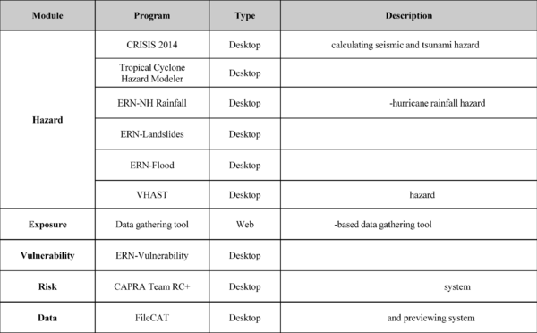
The modules are classified by topics related to hazard, exposure, vulnerability and risk assessment as shown in Figure G.1.

Figure G.1. CAPRA Platform modules

As shown in Figure G.2 all the outputs generated in any of the hazard modules are stored onto the *.AME files while exposure databases are stored onto ESRI shapefiles (*.shp). Finally, the vulnerability functions can be stored either in *.xml or ASCII format files that are then assigned in the CAPRA Team RC+ to each of the building classes included in the exposure database.

The CAPRA Platform is flexible in the sense that the hazard inputs can be generated using different modules that those that belong to the initiative with the only requisite that the hazard results are quantified using an scenario-based approach and saved in *.AME format that can be easily generated in *.xml files with the respective grids.

Figure G.2. CAPRA Platform input/output flowchart

The risk calculator of the initiative is the CAPRA Team RC+, which interface is shown in Figure G.3. The program is a parallelized probabilistic risk calculator with some GIS (geographical information system) capabilities where the different outputs generated in the hazard, exposure and vulnerability modules are added to the project. The program obtains the LEC for each of the portfolios and if several hazards are being considered, the LECs can be disaggregated.

CAPRA Team RC+ is an improved version of the original risk calculator program of the initiative known as CAPRA-GIS. Besides the parallelization process that can speed up to three times the calculation processing time, this new version has several improvements related to the flexibility and compatibility of it with different formats that are commonly used in the risk modelling community.

Figure G.3. CAPRA Team RC+ interface

The output of the CAPRA Team RC+ is an ASCII format file that contains the expected loss, variance and a-b values for the loss beta function for each of the scenarios that generate damage on the considered exposed dwellings as well as the LEC computed by 50 points from where different probabilistic risk metrics can be derived. Besides this, it is possible to obtain the PML plot directly from the program as shown in Figure G.4 where, if different hazards are considered in the assessment as in this example, a separate PML plot will be associated to each of them.

Figure G.4. CAPRA Team RC+ multi-hazard PML plot viewer

For expert users, a compact risk calculator known as the Capra Team PocketRC (see Figure G.5) is available when then, the users need to use as an input a file with the path of the hazard, exposure and vulnerability files to be used during the assessment but no visualizer is available. Results are obtained in exactly the same metrics and output files as in the CAPRA Team RC+. The main advantage of this tool is that computation time can be saved because of the lack of visualization.

Figure G.5. CAPRA Team PocketRC interface

As explained in the probabilistic risk assessment section, the physical risk results can be combined with lack of resilience and social fragility factors to have a holistic apporach for it. For this purpose, the Holistic Risk Calculator, EvHo (see Figure G.5) has been developed to incorporate the output files from the Capra Team RC+ (mainly related to urban risk assessments) into this framework.

Figure G.6. EvHo results interface

The CAPRA Initiative has been used in more than 20 countries around the world as shown in blue in Figure G.7 for detailed subnational and local risk assessments considering hazards of different origins besides being used for a fully probabilistic global risk assessment for more than 200 countries in the 2013 and 2015 versions of UNISDR Global Assessment Report on Disaster Risk Reduction.

Figure G.7. Countries where CAPRA has been used subnational and local risk assessments

The CAPRA Platform’s architecture has been thought to be modular, extensible and open, enabling the possibility of improving different inputs and existing contributions. That approach enables CAPRA to become a living instrument. CAPRA’s innovation results not only in another risk modelling platform but a community of disaster risk users that has been growing at worldwide levels through projects, training activities and workshops.

---

(²) www.filecat.org