Abstract
The trading and investment decision processes in financial markets becomes ever more dependent on the use of valuation and risk models. In certain, cases such as risk management, modelling practice has become so homogeneous that one is led to ask about the effect this has on the price formation process. Furthermore, should stable price patterns emerge from this, can sophisticated investors who have private information about the use and characteristics of these models make superior gains? The aim of this article is to test this hypothesis in a stylised market environment, where a strategic trader who trades on information about the valuation and risk management models used by competitors. Results show that for our particular market setting, such a strategy has an advantage over those that do not use this information.
Key words : Financial markets, Multi-agent simulation, Performativity, Higher-order strategies
1. Introduction
Recent advances in financial mathematics and the ready availability of computer power have led to an explosive growth in the use of simulation techniques in investment decision making. Investors, traders, and fund managers have grown accustomed to back up their decisions using valuation models and risk management systems. More so, hedge funds and proprietary desks take advantage of mathematical models to scan markets for profitable trade opportunities and nowadays automatic trading systems even act autonomously in financial markets, with only minor intervention from human actors.
As the use of mathematical models for valuation, forecasting, and risk measurement becomes more pervasive, it appears not at all unreasonable to speculate about the effect this might have on markets practice and price dynamics. MacKenzie (2004) talks here about the performativity of finance theory, in the particular case when well-established models are not merely describing market behaviour, but are instrumental in bringing into existence what they mean to describe. In a similar vane, it is possible to argue that as investment strategies in certain markets become ever more dependent on the usage of valuation and risk management models, price patterns will no doubt exhibit regularities that have not existed as such before, and which should become more pronounced the more market participants adopt a coarse grained or homogeneous set of modelling tools.
The aim of this article is to test this hypothesis in a stylised market environment similar to the one discussed in (Farmer, 1998), but with the addition of a strategic trader who utilises information on the valuation and risk management models used by the other market participants. Consequently as the decision making process of those relying heavily on models becomes more structured, sophisticated players such as our strategic trader might have a chance to take advantage of this by adjusting their strategies to take the pervasive model usage into account. Alternatively, a market regulator could use this knowledge with the intention of counteracting the negative externalities such a wide-spread, homogenous use of models could have in financial markets. We will however at this point not follow that particular line of inquiry.
2. Higher-Order Simulations
2.1 Exploiting Counterperformativity
In a recent article, MacKenzie (2003) noted that in the context of the 1998 liquidity crisis, modern risk management practice, and notably value-at-risk techniques, induced market interdependencies that lead to heightened price instability – a phenomenon that has also been commented on elsewhere (IMF, 1998; BIS, 1999; Mayer, 1999) – and, in some well-publicised cases, to large losses for the involved institutions. Although these problems have been put down by some commentators to inaccurate modelling hypotheses, it seems that in this particular case, risk models were counterperformative (MacKenzie, 2004) in the sense that they were a determining factor in creating market instability. Assuming a slightly relaxed definition of performativity, one can argue that the widespread, homogeneous use of any financial models, independently of their accuracy or correctness, ought to be constitutive of the price formation process, which, in some cases, generate adverse systemic responses.
In (Peffer, 2004; Llacay and Peffer, 2004) we have analysed the counterperformative effect that a widespread use of value-at-risk techniques has on the price dynamics and on the evolution of a trader population. In this article, we link (counter)performativity of valuation and risk management models to that of model-based investment strategies and in particular to the possibility of using higher-order strategies to gain a competitive advantage in tightly model-structured financial markets. Generally, agent interaction in financial markets is not strategic, which Morris and Shin (2000) associate with the fact that in normal times, financial markets are like roulette wheels, where the odds of placing a bet by a single player does not affect the riskiness of the gamble2. However, performativity – or more correctly counterperformativity – can severely affect or even invalidate these normality assumptions. And particularly in situations where investor behaviour is tightly linked to certain valuation and risk management models, market risk might take on a quality that is not adequately reflected in these very models. The question is then if in that case the counterperformative nature of some financial models, by reducing generic uncertainty and creating what Morris and Shin (2000) have called strategic uncertainty, allows sophisticated investors to make superior gains on their improved knowledge of the market structure.
2.2 Simulations of Simulations
The idea of directing one’s actions based on competitors’ strategic behaviour is not new, of course, and has been extensively dealt with in the game theory literature. Unfortunately, investment theory has little to say on strategic interaction in financial markets, although (Allen and Morris, 2001) discusses some noted exceptions. In fact, most models used in financial valuation, in particular those drawing on econometric or time series analysis, seem to dispense of the economic actor and its behavioural characteristics altogether or aggregate this into a number e.g. the counterparty credit risk. One of the many reasons why strategic interaction is apparently immaterial for such models is that in competitive markets, investors are considered mere price takers who cannot influence prices with their own trading activities anyway, and decisions therefore do not have to be based on competitors’ strategies.
In financial practice however, situations where market participants behave strategically with regard to others’ expectations are not uncommon. In a so-called sunspot panic for instance, a bank can become insolvent if depositors withdraw their cash solely because they think others will do so, and since in that case withdrawing one’s own funds is rational (Diamond and Dybvig, 1983). Asset bubbles are a further example of such phenomena and are brought about by beliefs, not founded in economic fundamentals, about future economic gains. There has been some interest recently in what are called global games (Morris and Shin, 2003), which acknowledge the importance of higher order beliefs (one’s beliefs about others’ beliefs about others’ beliefs and so on) in determining equilibrium outcomes of games with incomplete information.
To develop our argument, we start out from the idea of global games and apply it to situations where significant information is available about the structure of such beliefs. In particular, we assume that a large proportion of market participants’ beliefs about future events are closely related to the output from the valuation and risk measurement models they use. We view valuation, forecast, and risk models that investors and traders run on their computers as being simulations and, since we want to assess their market impact and strategic potential, make them the target of our own simulations. Following the notion of higher-order beliefs, we refer to such simulations of simulations as higher-order simulations, a concept that allows us to explore what market impact investors’ decisions have that are guided by simulations of other market participants’ behaviour, which in turn is guided by their own simulations.
3. The Methodology
The dominant modelling paradigm in economics and some areas of social sciences draws on the pivotal concept of rational choice, in which optimisation of agent satisfaction, conceptualised in the theory of expected utility and the consumer choice theory, plays a central role. However, representing half-way realistic investment models would be an onerous, if not impossible task inside a theoretic-analytical framework and we therefore pursue a different approach here altogether.
A growing number of researchers in the social sciences has moved their attention to multi-agent systems as a promising framework to model complex social interactions (Sawyer, 2003), and there has been some interest in employing this innovative approach to explain phenomena observed in financial markets (Chan et al., 1999; LeBaron, 1998). The most discernible feature which distinguishes MABS from other simulation techniques such as system dynamics modelling or Monte Carlo simulation lies in its use of multi-agent system as the fundamental reference framework within which to formulate models and run simulations.
Hence, to effectively address the question of higher order simulations in investment decision making, we present a simple multi-agent model of a stylised bond market where investment funds and relative value traders make investment decisions based on their proper valuation models and risk measurement techniques.
4. The Model
4.1 The Economic Environment
We consider a financial market for two bonds ![]() and
and ![]() in unrestricted supply, where
in unrestricted supply, where ![]() investment funds (IFs),
investment funds (IFs), ![]() reactive relative value traders (RRVTs), and
reactive relative value traders (RRVTs), and ![]() strategic relative value traders (SRVTs) are actively trading both securities using different valuation models. We assume that both bonds are substitutes in terms of their specifications but that for particular reasons which we won’t specify further, both trade at a price spread relative to each other. The investment funds act as fundamental investors, deriving the perceived value for both bonds from a private, exogenous signal they receive before each trading period. The liquidity of the bonds is given by
strategic relative value traders (SRVTs) are actively trading both securities using different valuation models. We assume that both bonds are substitutes in terms of their specifications but that for particular reasons which we won’t specify further, both trade at a price spread relative to each other. The investment funds act as fundamental investors, deriving the perceived value for both bonds from a private, exogenous signal they receive before each trading period. The liquidity of the bonds is given by ![]() and
and ![]() and their initial prices are set to
and their initial prices are set to ![]() and
and ![]() respectively.
respectively.
Agents place orders at discrete trading intervals where they decide how to change the make up of their portfolio based on the valuation models and, in the case where portfolio risk limits apply, on the Value-at-Risk (VaR) models. The capital that trading agents invest into the trading opportunities at each trading period is proportional to either a given constant or a utility-dependent factor c. In the latter case, agents gauge their past success based on a regret measure which will allow them to adjust the investment capital for the upcoming trading period.
Since the strategy of the relative value traders is based on the price difference between both instruments, we define the linear price spread as
4.2 The Market Price Dynamics
Prices ![]() and
and ![]() for both bond issues are set by a market maker in accordance with the following linear price formation rule, whereby prices have to rise (fall) in the presence of over-demand (over-supply) by an amount that is inversely proportional to the liquidity of the traded security
for both bond issues are set by a market maker in accordance with the following linear price formation rule, whereby prices have to rise (fall) in the presence of over-demand (over-supply) by an amount that is inversely proportional to the liquidity of the traded security
|
(4.1) |
where ![]() is the total time-
is the total time- ![]() excess order – the sum of all orders emitted in the time interval
excess order – the sum of all orders emitted in the time interval ![]() – of bond i and
– of bond i and ![]() is a constant liquidity factor that accounts for the depth of the market in the bond i. The disadvantage with this linear formulation is that prices can become negative, which could be avoided by using a log-price formulation for the price formation rule. Outstanding orders in any given trading interval are always filled at the quoted prices and the market maker absorbs the excess or covers the shortfall, adjusting the prices according to the impact function (4.1).
is a constant liquidity factor that accounts for the depth of the market in the bond i. The disadvantage with this linear formulation is that prices can become negative, which could be avoided by using a log-price formulation for the price formation rule. Outstanding orders in any given trading interval are always filled at the quoted prices and the market maker absorbs the excess or covers the shortfall, adjusting the prices according to the impact function (4.1).
4.3 First and Second Order Trading Strategies
In our model, a strategy is a rule by which an agent A determines the next-period order vector ![]() based on the information I he has
based on the information I he has
Zero-order strategies are those that take only information from the system environment into account. In the context of financial markets, zero order strategies may not seem particularly interesting but they are exemplified in those decisions where for instance macro-economic factors play a role. However, traders in our model will not use such strategies. Second order strategies are strategy rules that depend not only on information from the environment, but also on aggregation and individual, agent-related information, such as the type of valuation models competitors use. Between the zero and second order strategies lie those that are most pervasive in financial markets, namely the first order strategies that use macro-level, aggregate or systemic information to direct the agents’ decision process. Here, price and volatility information are perhaps the two most important market aggregates.
In the following we will introduce three types of market agents, two of which use first-order valuation strategies and a third type which uses second-order strategies based on the knowledge of models the other traders use.
4.3.1 Investment Funds (IFs)
Investment funds are so-called fundamental traders, who are not interested in historical price patterns of the securities, but in their intrinsic value. Each investment fund ![]() updates his perceived fundamental value of the bond i in accordance with an exogenous random walk of the form
updates his perceived fundamental value of the bond i in accordance with an exogenous random walk of the form
where the ![]() are drawn from the normal distribution
are drawn from the normal distribution ![]() , with agent-specific, time-independent drift and variance. In particular, investment funds’ value perception
, with agent-specific, time-independent drift and variance. In particular, investment funds’ value perception ![]() is modelled as a moving average over the past
is modelled as a moving average over the past ![]() fundamental values
fundamental values
The initial value ![]() is set to the price
is set to the price ![]() of bond i. Using a MA(m) price dynamics also allows the SRVT to make reasonably accurate value forecasts. Investment funds emit orders, whose magnitude is proportional to the difference between the actual price
of bond i. Using a MA(m) price dynamics also allows the SRVT to make reasonably accurate value forecasts. Investment funds emit orders, whose magnitude is proportional to the difference between the actual price ![]() and the perceived value
and the perceived value ![]() , and is also proportional to the available investment capital for their strategy
, and is also proportional to the available investment capital for their strategy
The capital factor ![]() is either a constant or inversely proportional to a measure of regret, which we introduce in section 4.4. Once the agents have calculated the bond orders for the current trading interval, they update their positions in both bonds
is either a constant or inversely proportional to a measure of regret, which we introduce in section 4.4. Once the agents have calculated the bond orders for the current trading interval, they update their positions in both bonds
In section 4.5, we will introduce VaR risk limits for the investors portfolios, which may restrict the total position the investment fund can take in bond i.
4.3.2 Reactive Relative Value Traders (RRVTs)
Reactive relative value traders are a special creed of momentum traders and hence belong to the class of technical traders. Their strategy is quite simple, and is based on the change in price spread ![]() between the two bonds. As in the case of the investment fund, the relative value trader places orders that are proportional to the capital factor
between the two bonds. As in the case of the investment fund, the relative value trader places orders that are proportional to the capital factor ![]() , which is either constant or reflects his idiosyncratic risk aversion and the confidence he places into his trading strategy
, which is either constant or reflects his idiosyncratic risk aversion and the confidence he places into his trading strategy
|
(4.2) |
The order of the second bond is determined so that the net cash outlay in the trade is zero
|
(4.3) |
Once the RRVT has determined the orders for both bonds, he will proceed to update the total portfolio positions according to
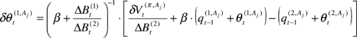
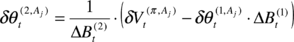
4.3.3 Strategic Relative Value Traders (SRVTs)
Strategic relative value traders base their trading strategy on a forecast of the orders of investment funds and reactive relative value traders. In the model as it stands at the moment, the strategic traders have knowledge of the past m orders ![]() placed by each one of the investment funds
placed by each one of the investment funds ![]() and know the capital factor
and know the capital factor ![]() each fund is using in their strategy. Given the past orders, the SRVT can infer the values
each fund is using in their strategy. Given the past orders, the SRVT can infer the values ![]() and hence calculate the expected value of the MA(m) indicator
and hence calculate the expected value of the MA(m) indicator
|
(4.4) |
from which the investment fund will calculate his next-period order, and where the ‘tilde’ denotes a random variable. Taking expectations on both sides of expression (4.4) then leads to the MA(m) estimate the SRVT uses to calculate the orders issued by the investment funds
The estimated total order issued by the investment funds is then determined by
The strategic relative value trader will then calculate the orders by the RRVTs in the current time period, which, knowing their capital factors, can be determined exactly and thus are equal to the one the RRVTs are calculating using (4.2) and (4.3). The total number of orders by RRVTs for both bonds is hence equal to
In some of the simulations where agents use VaR risk limits (see section 4.5 for details), order constraints can apply which the SRVT can take into account when estimating the orders the IFs and the RRVTs are likely to issue. In that case, the SRVT needs to estimate the next-period position of agent ![]() and determine whether a risk limit is likely to apply or not, based on the next-period forecast
and determine whether a risk limit is likely to apply or not, based on the next-period forecast ![]() of agent
of agent ![]() ’s portfolio volatility.
’s portfolio volatility.
Having determined the current period forecasts of the orders for both the investment funds and the reactive relative value traders, the SRVT will estimate the next-period prices ![]() and
and ![]() using the price dynamics discussed in section 4.2.
using the price dynamics discussed in section 4.2.
and a trend adjustment so that the final price estimate is equal to
|
(4.5) |
The strategic relative value trader issues orders for bond ![]() and
and ![]() based on the same spread momentum strategy used by the RRVTs, but with a next-period spread estimated using the bond price forecast (4.5)
based on the same spread momentum strategy used by the RRVTs, but with a next-period spread estimated using the bond price forecast (4.5)
Their next-period portfolio position is thus
4.4 Regret Adjustment of Agent Strategies
The market dynamics resulting from the trading activities in different agent populations is analysed in detail in sections 5.1 and 5.2 for the strategies outlined in the previous section. Up to this point, agents invested into their trading strategy independently of the actual success of that strategy. Since agents in our model cannot choose alternative strategies if theirs fail, they will want to reduce the capital outlay once it becomes apparent that the risk of loss is too great. To model this behaviour, we adjust the hitherto constant capital factor with an expected regret measure of the form
|
(4.6) |
where ![]() is the mean of total accumulated profits,
is the mean of total accumulated profits, ![]() is a scaling factor,
is a scaling factor, ![]() is one minus the strategy’s confidence level,
is one minus the strategy’s confidence level, ![]() is a measure for the investor’s risk aversion, and
is a measure for the investor’s risk aversion, and ![]() (
( ![]() ) stands for the frequency of loss (profit). Using the expected regret measure r, agents will determine at each trading interval the capital – represented by the factor c – they are prepared to invest into the trading opportunity
) stands for the frequency of loss (profit). Using the expected regret measure r, agents will determine at each trading interval the capital – represented by the factor c – they are prepared to invest into the trading opportunity
In order to determine the regret measure (4.6), agent ![]() first calculates the accumulated time-t profit
first calculates the accumulated time-t profit ![]() of his portfolio
of his portfolio
after which the confidence level is calculated following two different methods, a direct calculation of the profit frequency of a given strategy and a calculation in which we make the normality assumption for the accumulated profit.
With the direct method, agents determine their confidence level w.r.t. their strategy by calculating the ratio of profits to total traded volume
 ,
,where ![]() . In the case of the normality assumption, agent
. In the case of the normality assumption, agent ![]() calculates the mean
calculates the mean ![]() and variance
and variance ![]() of the accumulated profit and constructs a normal distribution in order to determine his confidence level
of the accumulated profit and constructs a normal distribution in order to determine his confidence level
with ![]() .
.
4.5 Portfolio VaR Limits
We are now adding a risk model to the set of models used by agents in their investment decision making process, with the intention of inducing a certain irregularity into the price dynamics in the bond market, thereby possibly increasing the possibilities for the strategic trader to gain an advantage compared to the two other types of traders, and in particular to the reactive relative value traders, since their strategies are comparable.
Currently agents determine the number of bonds they wish to buy or sell in a given trade interval using the strategy assigned to them. Since the market risk of their portfolio increases with the net position and the price volatility, we will impose VaR position limits which in effect curtail the risk of future losses. Value-at-Risk is a widely employed method to measure market risk of an investment portfolio based on the positions, volatilities, and correlations of the assets in the portfolio. Assuming that for a given portfolio ![]() and time horizon
and time horizon ![]() the P&L3
the P&L3 ![]() is distributed normally with mean
is distributed normally with mean ![]() and normalised variance
and normalised variance ![]() , we obtain the following estimate for the maximum loss within a confidence interval
, we obtain the following estimate for the maximum loss within a confidence interval ![]()
such that ![]() . After having determined their respective orders
. After having determined their respective orders ![]() , the time-t-1 change in value
, the time-t-1 change in value ![]() of the portfolio of agent
of the portfolio of agent ![]() is equal to
is equal to ![]() . Given a maximum loss limit
. Given a maximum loss limit ![]() for agent
for agent ![]() , the upper bound on the time-t value of the portfolio is equal to
, the upper bound on the time-t value of the portfolio is equal to
where we will use a confidence level of 99% or, equivalently, set ![]() . If this condition is not satisfied, the agent will reduce the time-t-1 orders to a level where the VaR risk limit condition is met and in a way that the proportion of the bonds in the portfolio does not change. Suppose that the time-t value of the portfolio exceeds the maximum permitted and that the difference between
. If this condition is not satisfied, the agent will reduce the time-t-1 orders to a level where the VaR risk limit condition is met and in a way that the proportion of the bonds in the portfolio does not change. Suppose that the time-t value of the portfolio exceeds the maximum permitted and that the difference between ![]() and the maximum time-t value and the residual value is denoted by
and the maximum time-t value and the residual value is denoted by ![]() , and that we need to reduce the time-t-1 orders with the asset proportionality factor defined as
, and that we need to reduce the time-t-1 orders with the asset proportionality factor defined as ![]() . In that case, the orders will have to be reduced by the following amounts
. In that case, the orders will have to be reduced by the following amounts
 ,
,

 ,
,
so that the VaR condition is satisfied for both bonds. The volatility of the two-bond portfolio ![]() is calculated taking into account the historical correlation between both bonds
is calculated taking into account the historical correlation between both bonds
with ![]() being the relative size of the position of asset
being the relative size of the position of asset ![]() , and the bond volatility at time t calculated over a window of size
, and the bond volatility at time t calculated over a window of size ![]() using the following standard expression
using the following standard expression
 ,
,and the correlations are calculated in the same window using a standard expression as in the case of the bond volatilities.
5. Market Simulations
By using a multi-agent simulation of the market described above, our aim is twofold. First, we want to illustrate the impact that a widespread use of valuation and risk models have on price formation and market stability. Second, and more importantly, we want to address the question of using simulations of competitors’ decision models to inform one’s investment strategies. In particular, we would like to appraise the effectiveness of using higher order simulations in the investment process for our particular market.
5.1 Case 1: A Population of Investment Funds and Reactive Relative Value Traders
In a first series of simulation experiments, we consider a trading context without the presence of higher order strategies, and hence a population consisting only of investment funds and reactive relative value traders. In each of the cases, the variable parameters of which are listed in table 5.1 below, 20 investment funds and ![]() reactive relative value traders buy and sell the two available bonds, and market prices are updated by a market maker absorbing order excesses and shortfalls as they arise over time. The number of trading intervals in each round is equal to 200 and a total of four experiments E1.1 – E1.4 have been carried out4. The initial price for both bonds is
reactive relative value traders buy and sell the two available bonds, and market prices are updated by a market maker absorbing order excesses and shortfalls as they arise over time. The number of trading intervals in each round is equal to 200 and a total of four experiments E1.1 – E1.4 have been carried out4. The initial price for both bonds is ![]() , the size of the volatility window for VaR calculations is
, the size of the volatility window for VaR calculations is ![]() , the drifts of the agent-specific, exogenous value processes are drawn from the uniform distribution
, the drifts of the agent-specific, exogenous value processes are drawn from the uniform distribution ![]() , and the volatility is equal to 0.2 for all the processes. All experiments have been carried out with both the capital factor set to 1 and with making it dependent on the regret measure discussed in section 4.4. The scaling factor
, and the volatility is equal to 0.2 for all the processes. All experiments have been carried out with both the capital factor set to 1 and with making it dependent on the regret measure discussed in section 4.4. The scaling factor ![]() used in the expression for the expected regret has been set to
used in the expression for the expected regret has been set to ![]() in all experiments and the risk aversion
in all experiments and the risk aversion ![]() of each agent is equal to
of each agent is equal to ![]() . No moving average is used to model the investment funds’ perceived fundamental value – or, equivalently, the window size has been set to
. No moving average is used to model the investment funds’ perceived fundamental value – or, equivalently, the window size has been set to ![]() . The constant parameters have been chosen so that the price dynamics is reasonable and no results have been included where prices diverge since our aim is to analyse higher-order strategies in a working market environment.
. The constant parameters have been chosen so that the price dynamics is reasonable and no results have been included where prices diverge since our aim is to analyse higher-order strategies in a working market environment.
VaR: agents using VaR position limits | ||||||||||||||||||||
|
Table 5.1: Parameter settings for case 1 |
5.1.1 Single RRVT, Low Liquidity, and no VaR (E1.1)
In this first experiment, a low liquidity environment increases price volatility and because of the overwhelming presence of investment funds, prices closely follow the random walk of the value process. In such an environment with erratically changing prices, relative value traders have little chance to make a living with their momentum-based spread strategy.
  | |
| Figure 5.1: Bond prices and price spreads for IFs and RRVTs | |
It is clear from the results that the relative value trader accumulates losses with passing time and that investment funds on average gain. However it should be noted that the IF-accumulated gains in figure 5.2 are averaged over all investment funds and that this can give the misleading impression that the IFs have a winning strategy, a fact which can be more clearly discerned from the strategy confidence levels shown in figure 5.2. In fact, as can be seen from the standard deviation of accumulated profits in figure 5.3, profits for individual investment funds are quite volatile and the confidence level seems to settle at around 0.5, the limit for a zero-sum game. The relative value trader’s confidence in his strategy however tends to zero as his loss making is gaining momentum.
  | |
| Figure 5.2: Accumulated profits and confidence level for IFs and RRVTs | |
In figure 5.3 one can observe that as the mean of accumulated profits for investment funds rises, so does the average standard deviation. Hence, although average profits for the investment funds rise, chances to make a loss at any given trading interval are only slightly smaller than those to make a profit, and the probability that the loss exceeds a given limit increases with time.
  | |
| Figure 5.3: Mean and standard deviation of accumulated profits for IFs and RRVTs | |
If instead of a constant capital factor, agents apply a variable, regret-dependent capital outlay, the profit outlook changes for the relative value trader and investment funds alike. Looking at the price time series for bond ![]() and
and ![]() , we can see that the price does not follow the value as closely as it did in the case where the capital factor was constant. In fact, comparing the average orders for bond
, we can see that the price does not follow the value as closely as it did in the case where the capital factor was constant. In fact, comparing the average orders for bond ![]() of this case with those of the case where
of this case with those of the case where ![]() , clustering of order excess and shortfall becomes apparent (figure 5.5).
, clustering of order excess and shortfall becomes apparent (figure 5.5).
  | |
| Figure 5.4: Bond prices and value processes for both bonds | |
  | |
| Figure 5.5: Shortfall and excess clustering for IFs | |
In a rising market, investment funds that have consistently believed that the asset is undervalued will have entered long positions, which in turn will have generated substantial profits for them, led to heightened confidence in their strategy and therefore contributed, through an increase in their capital factor, to even larger positions. Funds that on the other hand have, in the same rising scenario, believed that the asset is overvalued, will have entered a short position in the hope to make a profit when the prices return to their perceived valuation levels. In the meantime however, these funds will loose money and therefore reduce the capital they invest into the fundamental strategy. As shown for bond ![]() in figure 5.4, the influence of the longs in such an
environment can be so strong that they manage to push prices far beyond average valuation levels. The reason for this is that upward movements in prices increase demand in the asset by longs more than decreases in prices are able to increase the supply by shorts, because of the asymmetry created by the differing capital factors. Short-lived downward moves also do not alter significantly the confidence of longs in their strategy despite their making losses. If the downward pressure persists however, longs with substantial positions will reduce their marginal capital investment in the strategy and their influence fades, while the confidence of shorts will recover and their influence on prices will rise.
in figure 5.4, the influence of the longs in such an
environment can be so strong that they manage to push prices far beyond average valuation levels. The reason for this is that upward movements in prices increase demand in the asset by longs more than decreases in prices are able to increase the supply by shorts, because of the asymmetry created by the differing capital factors. Short-lived downward moves also do not alter significantly the confidence of longs in their strategy despite their making losses. If the downward pressure persists however, longs with substantial positions will reduce their marginal capital investment in the strategy and their influence fades, while the confidence of shorts will recover and their influence on prices will rise.
  | |
| Figure 5.6: Average confidence levels and capital factors for IFs and RRVTs | |
Comparing the RRVT confidence levels for a constant capital factor (figure 5.2) with the levels obtained in the case of agents making regret-adjusted marginal investment decisions (figure 5.6), one finds a noticeable increase in the proportion of positive payoffs for the relative value strategy to the point where it reaches the average level of investment funds. This is in stark contrast to the rapidly declining levels of confidence of the RRVT in the case of the constant capital factor. Although the RRVT is still making losses at the beginning of the trading round, these do not persist as in the constant factor case and profits recover after around 140 trading intervals.
The dynamics of the capital factors for the investment fund is more complicated altogether and shows a behaviour that is in line with our discussion on the regret-adjusted capital factor above. The left-hand graph in figure 5.7 shows all individual capital factors for the IFs and the RRVT. The right-hand graph shows the paths for the capital factors of two investment funds, where one can clearly discern how the perception of the adequacy of the fundamental strategy shifts from a high-confidence to a low-confidence level and vice-versa.
  | |
| Figure 5.7: IFs and RRVT capital factors and two individual paths | |
5.1.2 Single RRVT, High Liquidity, and no VaR (E1.2)
Setting the liquidity in the previous experiment of both bonds to higher values will smoothen the price time series and improve the profit potential of the relative value strategy, mainly because of the improved prediction accuracy of the next-period prices (see figure 5.8 below). Maximum absolute errors for instance are approximately five times as high in the low-liquidity scenario then in the case where ![]() .
.
  | |
| Figure 5.8: Comparing forecast errors of RRVT for the two cases of | |
Even in the case where the capital factor is constant, the relative value strategy shows much improved levels of confidence and accumulated profits do not show the downward trend they did in the previous example (see figure 5.9).
  | |
| Figure 5.9: Accumulated profits and confidence level for | |
5.1.3 Multiple RRVTs, Low Liquidity, and no VaR (E1.3)
In this experiment, the liquidity was reset to the value it had in E1.1 ( ![]() ) and the number of reactive relative value traders was increased from 1 to 20. In the case of a constant capital factor (
) and the number of reactive relative value traders was increased from 1 to 20. In the case of a constant capital factor ( ![]() ), prices tend to over- and undershoot the value process and the oscillatory behaviour tends to erode the profits of the RRVTs. Setting the capital factor proportional to the expected regret measure has a similar effect than it had in E1.1. Average accumulated profits and confidence levels are shown in figure 5.10 for both investment funds and relative value traders.
), prices tend to over- and undershoot the value process and the oscillatory behaviour tends to erode the profits of the RRVTs. Setting the capital factor proportional to the expected regret measure has a similar effect than it had in E1.1. Average accumulated profits and confidence levels are shown in figure 5.10 for both investment funds and relative value traders.
  | |
| Figure 5.10:Accumulated profits and confidence levels for variable capital factor and NRRVT =20 | |
5.1.4 Multiple RRVTs, Low Liquidity, and VaR Risk Limit (E1.4)
Agents will now use value-at-risk position limits to constrain the order the issue at each trading interval. We have set the maximum acceptable market risk to levels where this induces a marked rise in volatility in the bond price process and acknowledge the fact that the oscillations this is provoking might be extreme, but nevertheless underline our case. Under such a scenario, bond spreads can change abruptly and even in the case of using a variable capital factor, the RRVTs fare very poorly (see figure 5.11).
  | |
| Figure 5.11: Price spread and confidence levels when IFs use VaR | |
When introducing a strategic relative value trader into our market (see section 5.2), we will see that investing into the relative value strategy whilst being able to take into account possible future VaR adjustments can drastically improve profit outlook compared to the naïve relative value strategy used by the RRVTs.
5.2 Case 2: Adding a Strategic Relative Value Trader
In this second set of simulation experiments, we will add an additional trading agent who uses a higher order relative value strategy to trade on improved knowledge of the market structure, in particular of the models that other agents – reactive relative value traders and investment funds – use to determine their orders. Similar than in the previous case, 20 investment funds trade in each of the experiments E2.1 – E2.4 with ![]() reactive relative value traders, with the main difference that a single strategic relative value trader is also actively trading in the market, although in sizes that have only little impact on prices. In each trading interval, bond prices are again set by the market maker according to the price impact function (4.1). Each experiment6 consists of 200 trading intervals, except for E2.4, which compares profits of the SRVT with those of the RRVTs over a sample of 10,000 trading rounds (each consisting again of 200 trading intervals). The initial price for both bonds is, as in case 1,
reactive relative value traders, with the main difference that a single strategic relative value trader is also actively trading in the market, although in sizes that have only little impact on prices. In each trading interval, bond prices are again set by the market maker according to the price impact function (4.1). Each experiment6 consists of 200 trading intervals, except for E2.4, which compares profits of the SRVT with those of the RRVTs over a sample of 10,000 trading rounds (each consisting again of 200 trading intervals). The initial price for both bonds is, as in case 1, ![]() , the size of the volatility window for VaR calculations is
, the size of the volatility window for VaR calculations is ![]() , the drifts of the exogenous value processes are drawn from the uniform distribution
, the drifts of the exogenous value processes are drawn from the uniform distribution ![]() , and the volatility is equal to 0.2 in each case. All experiments except E2.4 have been carried out with the liquidity factors
, and the volatility is equal to 0.2 in each case. All experiments except E2.4 have been carried out with the liquidity factors ![]() . Simulation runs have been conducted both with a constant capital factor equal to 1 and with making it dependent on the regret measure discussed in section 4.4. The scaling factor
. Simulation runs have been conducted both with a constant capital factor equal to 1 and with making it dependent on the regret measure discussed in section 4.4. The scaling factor ![]() used in the expression for the expected regret has again been set to
used in the expression for the expected regret has again been set to ![]() in all experiments.
in all experiments.
m: moving-average window size; VaR: agents using VaR position limits | |||||||||||||||||||||||||
|
Table 5.2: Parameter settings for case 2 |
5.2.1 Single RRVT, small MA (m=1), and no VaR (E2.1)
Parameters of this first experiment are identical to those in E1.1, however with the difference that a strategic relative value trader has been added to the market. The strategies of both the RRVT and the SRVT are fundamentally the same, but whereas the RRVT uses two past values of the bond price spread to calculate his orders, the SRVT makes a prediction of next period’s spread based on the knowledge she has on the strategies – or models – used by both the RRVTs and the IFs to calculate her bond orders. Results show that confidence levels of the SRVT are lower than those by the RRVTs by a factor of 1.5 in the case of a constant capital factor (c =1), although this is an exceptional circumstance in all the results that follow. In this particular situation, with only one RRVT actively trading in the market and the capital invested in the strategy time-invariant, confidence levels are very low and do not exceed 40%, thus making both strategies unattractive compared to a fair gamble.
  | |
| Figure 5.12: Accumulated profits and confidence levels for variable capital factor | |
Similar to the previous case, an environment with predominantly investment funds is not very conducive for the relative value trading strategy of either the RRVT or the SRVT. Given that the prices follow the random walk of the fundamental values closely, there is not much room for manoeuvre to exploit the direction of spread movements. Nevertheless, we can observe in figure 5.12 that the SRVT has a slight advantage over the RRVT and that her confidence in the higher-order strategy is quite high. Hence, although average accumulated profits are lower than for the IFs, the little profit they make is more certain. We have already mentioned in experiment E1.1 that accumulated profit graphs show average values and that profits change considerably from one investment fund to another. Confidence levels are only slightly higher then 50% also in this experiment so that the IF strategy does not fair much better than a fair game.
5.2.2 Multiple RRVT, large MA (m=15), and no VaR (E2.2)
In this experiment, there are now twenty reactive relative value traders compared to only one in the previous experiment E2.1, and investment funds calculate their fundamental value forecasts using a moving average window of ![]() . The increase in the MA window size will induce a certain structure in the market – compared to the random walk of the fundamental value – that the strategic trader can exploit. In fact, as can be seen in figure 5.13, the price predictions the SRVT does based on a deeper knowledge of the strategies used by the other traders are much more accurate than those of the RRVT who uses a simple historical momentum strategy. While the RRVTs do not seem to make any substantial profits, the strategic trader does very well for both constant and variable capital factor and her low prediction error allows her to make steady gains which in turn pushes her confidence level to 100%. In this second case, when agents adjust their investment capital in accordance with the regret measure (4.6), the price behaviour becomes much less oscillatory, which is beneficial for the relative value traders, and in particular for the SRVT.
. The increase in the MA window size will induce a certain structure in the market – compared to the random walk of the fundamental value – that the strategic trader can exploit. In fact, as can be seen in figure 5.13, the price predictions the SRVT does based on a deeper knowledge of the strategies used by the other traders are much more accurate than those of the RRVT who uses a simple historical momentum strategy. While the RRVTs do not seem to make any substantial profits, the strategic trader does very well for both constant and variable capital factor and her low prediction error allows her to make steady gains which in turn pushes her confidence level to 100%. In this second case, when agents adjust their investment capital in accordance with the regret measure (4.6), the price behaviour becomes much less oscillatory, which is beneficial for the relative value traders, and in particular for the SRVT.
  | |
| Figure 5.13: Forecast error for RRVTs and SRVT (constant capital factor) | |
  | |
| Figure 5.14: Accumulated profits and confidence levels for variable capital factor | |
5.2.3 Multiple RRVT, large MA (m={1, 15}), and VaR Risk Limit (E2.3)
Our aim with this experiment is to analyse the effect that a VaR risk management model for IFs has on the price dynamics and the trade profitability. As we have seen in experiment E1.4, relatively low VaR limits tend to lead to a volatile price behaviour, which we have seen is affecting in particular the profitability of the relative value trader. In this experiment, we will analyse the results obtained by the strategic trader under two different scenarios. In a first simulation run the SRVT disregards the fact that the investment funds employ a VaR strategy to limit their positions and will face similar problems of making a profit than do the reactive relative value trader. In the second scenario, the SRVT has knowledge of the investment funds’ VaR strategy and incorporates this into her valuation model.
  | |
| Figure 5.15: Accumulated profits and confidence levels for variable capital factor (incl. VaR) | |
In the first case, figure 5.15 shows that the success of SRVT’s investment strategy suffers under the abrupt price changes induced by the use of VaR on behalf of the investment funds, even though these use a moving average model of the assets’ fundamental value (note that when the IFs used a moving average with a window of ![]() in experiment E2.2, this was clearly beneficial for the profitability of the higher-order strategy of the SRVT).
in experiment E2.2, this was clearly beneficial for the profitability of the higher-order strategy of the SRVT).
  | |
| Figure 5.16: Price spread and accumulated profits for variable capital factor | |
However, in the second scenario where the strategic relative value trader includes the knowledge of the investment funds’ VaR strategy into her own valuation model, the profitability outlook changes drastically (figure 5.16). Even in the case where ![]() , the
, the
SRVT makes a profit. From figure 5.18, one can see that the forecast errors are much smaller than for the RRVT, which is also reflected in the 100% confidence level that the higher-order strategy attains in this environment, both with a constant and a regret- dependent capital factor (figure 5.17). Although the forecast errors of the RRVT are generally small for a variable capital factor (figure 5.19), they become very large when the investment funds adjust their holding in accordance to their VaR position limits (see figure 5.16).
  | |
| Figure 5.17: Confidence levels for constant and variable capital factor | |
  | |
| Figure 5.18: Forecast error for RRVTs and SRVT (constant capital factor) | |
  | |
| Figure 5.19: Forecast error for RRVTs and SRVT (variable capital factor) | |
5.2.4 Temporal and Cross-Sectional Analysis (E2.4)
We will now present the results of a simple temporal and cross-sectional analysis of the relative performance of both the reactive relative value strategy of the RRVT and the higher-order relative value strategy of the SRVT. Furthermore, in a first set of trading rounds, the investment funds do not use VaR as a position limit, whereas in a second set, the investment funds choose their positions in accordance with the stipulations of their VaR risk model. For the purpose of this simple statistical analysis “by inspection”, we construct histograms for absolute profit differences between the RRVT and the SRVT strategy for both the cases where VaR is used and where no risk position limits are enforced.
Both cases with and without VaR are generated by a set of 10,000 trading rounds, each consisting of 200 trading intervals. There are 20 investment funds and 10 reactive relative value traders trading in the market, where the liquidity factor ![]() has been set equal to 2, and where the VaR limit has been set to
has been set equal to 2, and where the VaR limit has been set to ![]() in the cases where investment funds use a VaR position limit. The temporal histograms are constructed by averaging the differences of RRVT and SRVT profits for two particular paths and repeating this procedures for all profit path pairs in the set of 10,000 trading rounds. Similarly, the cross-sectional histograms have been generated by summing the differences of RRVT and SRVT profits at each time point over all 10,000 paths and repeating the averaging procedure for all 200 time buckets.
in the cases where investment funds use a VaR position limit. The temporal histograms are constructed by averaging the differences of RRVT and SRVT profits for two particular paths and repeating this procedures for all profit path pairs in the set of 10,000 trading rounds. Similarly, the cross-sectional histograms have been generated by summing the differences of RRVT and SRVT profits at each time point over all 10,000 paths and repeating the averaging procedure for all 200 time buckets.
 |
 Figure 5.20: Temporal and cross-sectional histograms of accumulated profit differences |
We can see from these results that the higher-order strategy of the SRVT consistently outperforms that of the RRVT. The histogram of temporal differences brings perhaps the more relevant characteristic of profit differences to the fore. The profit differences between two individual paths can be thought of as a “strong” indicator of strategic superiority, since unlike in the case of cross-sectional averaging we compare two actual realisations of the profit process. The cross-sectional histogram on the other hand provides merely a probabilistic picture – it is a “weak” indicator” – of the strategic advantage of the SRVT, since it averages profit differences for all paths at each point in time. In the case where the IFs are not using a VaR model and price behaviour is not erratic because of this, the advantage of the SRVT over the momentum strategy of the RRVT is only small. However, as soon as the investment funds use their VaR model to set position limits, we see that the SRVT strategy pays off considerably. In particular the temporal histogram – our strong indicator – clearly shows that now where the investment funds use a VaR limit, the SRVT has gained the upper hand by using a higher-order strategy which takes into account the models used by the other market players.
6. Conclusions and Future Research
In this article we have applied the concept of arbitrary but non-random performativity, as a natural extension of MacKenzie’s Austinian performativity, to a situation where investors employ higher-order strategies to trade on model-induced price patterns in a two-asset financial market. The extended concept of performativity used here includes situations where models do not perform their stated hypotheses, but where the resulting market practices and patterns assume nevertheless a stable existence and where stakeholders are perhaps reluctant to substitute the current technology with a better, but less known one. We have demonstrated that in a stylised economic environment in which the decision making process of fundamental and relative values traders is tightly linked to the use of valuation and risk management models, traders that employ second-order strategies that explicitly account for the use these models by competitors, can in some cases profit from the emerging price patterns.
The exploration of the implications of our market model was done using a somewhat watered-down version of what are called multi-agent based simulations – one would expect agents at least to engage in some form of communication in a real multi-agent simulation, or that they should exhibit a certain level of autonomy. There are initially two types of traders operating in the market: investment funds and reactive relative value traders, which employ a fundamental strategy and a technical strategy respectively. In conjunction with the simple linear price impact function we have used, the combination of the two types of trading behaviour can be viewed as a minimal set-up in which a reasonable price dynamics emerges. The investment funds – the fundamental traders – employs private, stochastic information of the value of the two bonds to decide if these are overvalued or undervalued, and to place their orders accordingly. Reactive relative value traders on the other side employ a simple spread momentum strategy to calculate their orders. Although the RRVT strategy is self-fulfilling on its own – it always forces prices into a profitable direction – this changes when investment funds with their stochastic value process invade the market. The more volatile the price process, the worse does the momentum strategy fare in an IF-invaded population, which has been demonstrated in the experiments E1.1 – E1.4.
To test the hypothesis of the exploitability of model-induced market structures by higher-order strategies, we have then introduced a third type of trader equipped with such a strategy into our market. Her strategy was basically the same than that of the reactive relative value trader, but instead of constructing a historical measure of spread momentum, this strategy included superior knowledge about the other market players’ valuation and risk management models and constructed a momentum measure based on a forecast of market orders. In case 2, we have seen throughout all experiments that the strategic relative value trader not only fares better in terms of absolute profitability than the RRVTs, but that the profit she makes with her enhanced strategy is worth more than the profit she would make with the naïve relative value strategy since, looking at the confidence levels, the risk attached to positive payoffs in the case of the higher-order strategy is lower than that of the naïve momentum strategy. In summary, the higher-order strategy benefits from an increase in the number of RRVTs, a better predictability of IF orders (from an increase in the size of the moving average window), a variable capital factor, and an increase in price volatility through the use of VaR position limits when the use of VaR models is known by the SRVT.
Two directions of future research are indicated at this point. Firstly, the strategy used by the SRVT has been chosen arbitrarily and changes in the strategy were not possible, except through an adjustment of capital outlay via the regret measure. We need to understand better – but always in the context of this stylised market with its particular price dynamics – how a successful strategy construction and selection process can be integrated in our model. In particular, the implications of the base strategies employed by investment funds and RRVTs has to be understood much better in order to gauge the results obtained after including a higher-order strategy. The higher-order strategies themselves have to be constructed in a systematic fashion and SRVTs need to be equipped with a strategy selection mechanism. Secondly, the model used here is indeed very stylistic, and in order to create a more realistic trading environment with heterogeneous and possibly (semi-)autonomous agents, we need to move away from the equation-based, analytically motivated evolutionary economics framework towards a more flexible, multi-agent systems framework which, although embracing working concepts from evolutionary economics, also allows for the efficient representation of agent autonomy and sociality.
7. References
Allen, F. and Morris, S. (2001). “Finance Applications of Game Theory.” In Chatterjee, K. and W. Samuelson (eds.), Advances in Business Applications of Game Theory, Kluwer Academic Publishers, 17-48.
BIS (1999). “A Review of Financial Market Events in Autumn 1998”, Bank for International Settlements, Basel.
Chan, N. T., LeBaron, B., Lo, A. W., Poggio, T., (1999). “Agent-Based Models of Financial Markets: A Comparison with Experimental Markets”, Center for eBusiness @ MIT, MIT Sloan School of Management.
Diamond, D. W., and Dybvig, P. H. (1983). “Bank runs, deposit insurance, and liquidity. Journal of Political Economy”, vol. 91 (June), 401–419. Reprinted in Federal Reserve Bank of Minneapolis Quarterly Review, vol. 24, No. 1, Winter 2000, 3–13.
Farmer, J.D. (1998). “Market Force, Ecology and Evolution.” Santa Fe Institute Working Paper No. 08-12-117.
IMF (1998). “World Economic Outlook and International Capital Markets”. Interim Assessment - December 1998, International Monetary Fund, Washington D.C.
Llacay, B. and Peffer, G. (2004). “Modelo evolutivo del impacto de técnicas VaR en los mercados financieros.” In 7th Spanish-Italian Meeting on Financial Mathematics, 8-9 Julio 2004, Cuenca.
LeBaron, B. (1998). “Agent Based Computational Finance: Suggested Readings and Early Research”, Journal of Economic Dynamics and Control, vol. 24, 679-702.
MacKenzie, D. (2004). “An Engine, not a Camera: Finance Theory and the Making of Markets”, MIT Press forthcoming.
MacKenzie, D. (2003). “Long-Term Capital Management and the Sociology of Arbitrage”, Economy and Society, forthcoming.
Mayer, M. (1999). “Risk Reduction in the New Financial Architecture”, Public Policy Brief No. 56, The Jerome Levy Economics Institute of Bard College.
Morris, S. and Shin, H. S. (2000). “Market Risk with Interdependent Choice”, Conference on Liquidity Risk, Frankfurt, 30 June - 1 July 2000.
Morris, S. and Shin, H. S. (2003) “Global Games: Theory and Applications.” In Dewatripont, M., L. Hansen and S. Turnovsky (eds.) Advances in Economics and Econometrics (Proceedings of the Eighth World Congress of the Econometric Society), Cambridge University Press.
Peffer, G. (2004). “The Effects of VaR Position Limits on Endogenous Price Formation in Financial Markets.” In 7th Spanish-Italian Meeting on Financial Mathematics, 8-9 Julio 2004, Cuenca.
Persaud, A. (2000). “Sending the Herd off the Cliff Edge”, Erisk, December 2000.
Sawyer, R. K. (2003). “Artificial Societies: Multiagent Systems and the Micro-Macro Link in Sociological Theory”, Sociological Methods and Research, vol. 31, No. 3, 325-363.
(1) First version submitted to the Internacional Conference on Modelling and Simulation – ICMS’04 (Valladolid, Spain, 22-24 September 2004)
Paper under revision for submission to JASSS (Journal of Artificial Societies and Social Simulation)
(2) It should however be noted that the analogy with competitive financial markets is not complete since the actions of market participants are constitutive of the outcome – the price in this case – although the decision process does not account explicitly for the beliefs about other investors' strategies and beliefs.
(3) Profit and loss
(4) Each experiment uses the same set of random numbers so that the results remain comparable
(5) The liquidity factor 12px is equal to 2 in this experiment
(6) Experiments E2.1 – E2.3 use the same underlying random number sequences to ensure that the results are comparable
Document information

Published on 01/01/2004
Licence: CC BY-NC-SA license
Share this document
Keywords

claim authorship
Are you one of the authors of this document?