An arctic low-energy house as experimental setup for studies of heat dynamics of buildings

Abstract

This paper addresses the difficulties in pinpointing reasons for unexpectedly high energy consumption in construction, and in low-energy houses especially. Statistical methods are applied to improve the insight into the energy performance and heat dynamics of a building based on consumption records and weather data. Dynamical methods separate influences from outdoor temperature, solar radiation, and wind on the energy consumption in the building. The studied building is a low-energy house in Sisimiut, Greenland. Weather conditions like large temperature differences between indoors and outdoors throughout long winters, strong winds, and very different circumstances regarding solar radiation compared to areas where low-energy houses are usually built, make the location very interesting for modeling and testing purposes. In 2011 new measurement equipment was installed in the house, which will be used to develop more detailed models of the heat dynamics and energy performance in relation to different meteorological variables, heating systems, and user behavior. This type of models is known as a graybox model and is been introduced in this paper.

Keywords

Low-energy houses ; Heat dynamics ; Arctic climate ; Statistical modeling ; Graybox modeling

1. Introduction

Increasing consciousness of the impact of human activities on the global environment – namely the consequences of emissions of greenhouse gases – has lately led to political goals of lowering energy consumption and switching to more sustainable energy supply systems. In buildings, this calls for improved methods for assessment of energy performance and characterization of heat dynamics.

In order to lower costs of collecting digital consumption data and for the consumer to be able to monitor his or her consumption pattern and maybe even adapt to price fluctuations, online data collection devices such as “Smart Meters” are getting increasingly common in dwellings. They typically monitor and log at least one consumption variable and possibly indoor climate variables. Already in Westergren et al. (1999) a framework is developed to estimate physical parameters of buildings based on weather and consumption data, and the energy consumption is modeled for a sample of buildings. In Mortensen and Nielsen (2010) rather simple methods are presented on how to estimate UA-values, gA-values and sensitivity to wind speed of buildings using only consumption and weather data. In Bacher et al. simple lowpass filters are applied to inputs and outputs in order to obtain reliable predictions of heat consumption in buildings on time intervals down to 1 h.

Discrete-time dynamical models have a large potential for use on automated and standardized measurements. ARMAX (Autoregressive Moving Average with eXogeneous inputs) models are a wide class of dynamical linear models. Norlén (1990) implements a recursive algorithm to estimate the UA-value of a test cell with ARMAX models, and in Jiménez et al. (2008a) ARMAX models are used on data from a test wall.

More detailed information about the heat dynamics of a building can be achieved by applying continuous-time models such as graybox models to data of higher resolution. This has been done for a part of a highly insulated building in Madsen and Holst (1995) . In Andersen et al. (2000) it was applied on a multi-room building, and Bacher and Madsen (2011) present a method for a consistent model selection procedure.

In 2005, a low-energy house was inaugurated in Sisimiut, Greenland. The objective was to build a house with very low energy consumption for heating, which should inspire the development of energy-efficient housing in Greenland and demonstrate the potentials for energy efficiency in a house which should also be a leading example of good indoor thermal environment. The house and its objective was also to be presented in Norling et al. (2006) . Therefore the current paper will only briefly introduce the building and then focus on how well the house has lived up to its performance targets, and which challenges it has incurred. Some preliminary performance results were presented also in Rode et al. (2009) , but significant improvements have occurred since then. The statistical analysis will be performed on data from before and after the work was conducted on the building and the results will be compared.

Apart from improvements on the energy performance of the envelope, the building has been equipped with numerous sensors and control equipment for conducting experiments in the building. Long winters of low outdoor temperatures give a high signal/noise ratio and ease planning of experiments. The modern design of the building with a high level of insulation, large window areas, and floor heating makes it interesting for studies of heat dynamics of modern low-energy construction. Moreover, it consists of two symmetrical apartments which enable studies of the influence of occupancy.

This paper presents results of statistical modeling of historical consumption data from the house in order to quantify the alleged improvement of the building envelope. It also describes the new measurement setup, and finally presents suggestions for obtaining more detailed heat dynamic models. The paper is structured in the following way: Section 2 gives a brief presentation of the low-energy house, Section 3 describes a statistical methods for analysis of data before and after the repair work on the building. Section 4 lines out plans for future experiments and analysis, and finally conclusions are given in Section 5 .

2. Description of the house

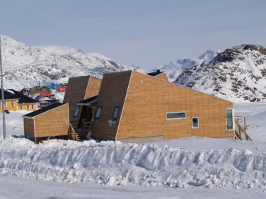
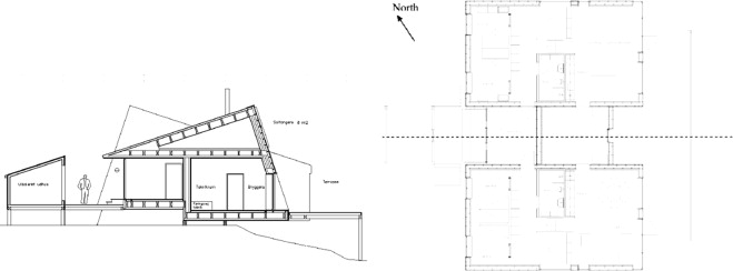
A target for the house was that the energy consumption for heating and ventilation should be only half of that permitted by the 2006 version of the Greenlandic Building Regulations: 230 kW h/m² /yr (Government of Greenland, 2006 ). Furthermore, considering that the house was planned to have a ventilation system with heat recovery – something that was not assumed for residential dwellings in the building regulations – the target value 80 kW h/m² /yr was chosen. Building energy simulations were executed to substantiate that this level of annual energy consumption was possible. The means to reduce the energy consumption in comparison with common Greenlandic houses have been to use extra insulation in floors, exterior walls and the roof. Advanced windows have been used with low energy glazing using normally 3 layers of glass. A solar collector has been installed on the roof for domestic hot water heating. The house has been orientated to exploit the light and its geometry optimizes the daylight absorption. The ventilation system is supplied with a counter-flow heat exchanger that uses the warm exhaust air to preheat the cold inlet air. Sisimiut is the second largest city of Greenland (5500 inhabitants) located on the west coast just 42 km north of the Polar Circle. The mean average temperature is around 6 °C in summer and around −13 °C in the winter months. The number of heating degree days is around 8000 K-days (base 19 °C). The house is approximately 200 m² and is made as a semi-detached house, where the two living areas are built on each side of the boiler room and an entrance hall. Figure 1 shows a picture of the house, and Figure 2 shows the cross section and floor plan. One of the two dwellings serves as home for a family, while the other is used as a guest house for visitors and for research experiments.

Figure 1. Photo of the low-energy house in Sisimiut as seen from the west.

Figure 2. Cross section and floor plan of the low-energy house. The house is built as a double house with common scullery/boiler room and entrance hall.

2.1. The building envelope

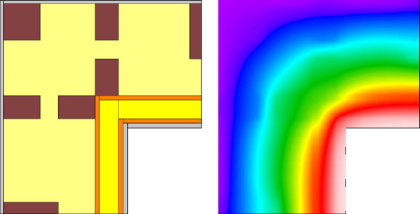
The building is generally made as a wood frame construction. The inhabited part is all on one floor, which is distributed over two slightly displaced levels, and there is a cold attic above the whole building, and an open crawl space below. The heat loss due to thermal transmittance of the building envelope constructions is kept at a minimum by using large insulation thicknesses and wooden posts and girders in two separate layers that do not touch each other, so thermal bridges are practically eliminated, see Table 1 and Figure 3 . As it can be seen from Table 1 all the constructions have U-values below the demands.

Table 1. Calculated U-values of the different constructions compared with the demands from the Greenlandic Building Regulations (GBR). The values include thermal bridge effects.

Construction	Floor	Walls	Roof
Insulation thickness (mm)	350	300	350
U-value calculated (W/m2 /K)	0.14	0.15	0.13
U-value GBR 2006 (W/m2 /K)	0.15	0.20	0.15

Figure 3. Wood based structural members near a corner of the building are configured such that thermal bridges are avoided. To the right: a plot of the calculated temperature distribution around the corner. The calculated linear thermal transmission coefficient is ${\textstyle \psi =0.015\quad W/(m\quad K)}$ .

2.2. Windows

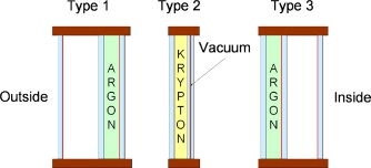
Three types of glazing units are used in the low-energy house:

Type 1- 1+2 solution: Made of one single glass layer with a hard low-emission coating and a sealed unit with two glass layers.

Type 2- Combined double energy glazing and a vacuum glazing unit.

Type 3- 2+1 solution: Made of a sealed unit with two layers of glass and a separate single layer of glass with a hard low emission coating.

The three types of glazing units are shown in Figure 4 . Data for the glazing units are shown in Table 2 . The net energy gain is calculated as a mean value of windows oriented north, east, west and south for a reference house.

Figure 4. The three glazing units used in the low-energy house.

Table 2. Heat transmission coefficient (${\textstyle U_{g}}$ , ${\textstyle U_{w}}$ ), solar energy transmission (${\textstyle g_{g}}$ , ${\textstyle g_{w}}$ ) and net annual energy gain (${\textstyle Q_{g}}$ , ${\textstyle Q_{w}}$ ). Index ${\textstyle g}$ for glazing and ${\textstyle w}$ for window.

Type	${\textstyle U_{g}}$ (W/(m2  K))	${\textstyle g_{g}}$ (–)	${\textstyle Q_{g}}$ (kW h/m2 )	${\textstyle U_{w}}$ (W/(m2  K))	${\textstyle g_{w}}$ (–)	${\textstyle Q_{w}}$ (kW h/m2 )
1: 1+2	0.7	0.45	172	1.0	0.30	−17.3
2: 2+Vac.glaz	0.7	0.40	136	1.1	0.27	−59.3
3: 2+1	0.8	0.56	228	1.1	0.47	67.1

2.3. Heating system

The low-energy house is constructed with a hydronic floor heating system based on PEX-tubes installed in aluminum plates just below the wooden floor boards. The floor heating system in the bathrooms is based on PEX-tubes cast in the concrete. The ventilation system is equipped with a heating coil which is positioned in the supply air duct after the heat exchanger. The heating coil is meant to ensure that the air supply is at a minimal temperature of 18 °C. The ventilation systems heating coil is based on the same hydronic system as the floor heating.

Hot water for the floor heating and heating coil is supplied from an oil furnace, which is located in the boiler room of the house. Heat for the domestic hot water comes from a solar collector. The oil furnace supplies back up heat in periods when the solar heating is insufficient. Finally, a radiator in the entrance hall is meant to be heated with excess heat from the solar collector system when available.

2.4. The ventilation system

Mechanical ventilation with heat recovery in cold climates can present problems with ice formation in the heat exchanger. When warm humid room air is brought in contact with the cold surfaces of the exchanger (cooled by the outside air), the moisture in the exhaust air condenses in the heat exchanger. If the outside air is below freezing, the water vapor will freeze, resulting in a larger air flow resistance on the exhaust side of the exchanger, which in turn decreases the air flow. The decrease in the amount of warm air through the exchanger will result in the exchanger being cooled further, and eventually the system will become fully blocked with ice and stop. This problem can be prevented by preheating the inlet air before it reaches the exchanger. This will however result in extra energy consumption and higher installation costs, and is therefore not an optimal solution.

A new design of a heat recovery unit was developed for the low-energy house in Sisimiut in cooperation between EXHAUSTO A/S and the Technical University of Denmark. The dimensions of the unit are length 1760 mm, width 930 mm and height 660 mm. The unit consists of two highly efficient aluminum counter flow heat exchangers coupled in a serial connection. A damper is able to switch the air flow direction through the units. When ice formation starts to reduce the air flow in the coldest exchanger, the air flow direction is switched. The exchangers, damper and filters are mounted in a cabinet with 50 mm insulation, although the unit is recommended to be placed in a heated place to minimize risks of frost damage from the condensing water. A diagram of the system is shown in Figure 5 . The theoretical temperature efficiency of the heat recovery unit is approximately 90%.

Figure 5. Diagram of the heat recovery unit with two heat exchangers. A valve and a timer switch the flow direction when ice formation reduces the air flow.

2.5. The solar collector

Solar hot water panels installed on the low-energy house constitute a flat plate collector. It has a total surface area of 8.1 m² and the system is able to collect 1700 kW h/yr. This covers approximately 57% of the hot water consumption of the house. The house and its inhabitants use around 150 L of hot water per day. The solar collector faces south-east and is tilted 70° from horizontal to have the optimal position in relation to the sun.

3. Linear modeling of existing data

Since the completion of the house, consumption and some indoor climate variables have been measured. The consumption recordings consist of common oil consumption and electricity consumption recordings for each apartment and for common areas. For the ventilation and heating systems, all inlet and outlet flows and temperatures have been measured. Moreover, measurements have been taken for temperatures and relative humidity both indoors and in some construction parts. Consumption recordings are cumulative, temperature and flow measurements are instant, and all data were logged every hour. Unfortunately, the measurement recordings have been interrupted, which limit the periods which can be used for modeling.

Two periods of approximately 2.5 months each have been chosen for analysis. The first period starts on September 1, 2009 while the second starts on February 1, 2010. Mending had been carried out between these two periods so the house was expected to perform better – namely be tighter and have a better control of the heating – in the second period.

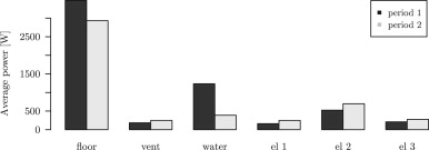
A first comparison of the energy consumption for the two periods is seen in Figure 6 . The largest power consumption is in floor heating which has been reduced by 545 W on an average or more than 15%. The ventilation heating is in general only 510% of the contribution from floor heating but it has increased by around 35%. Energy consumption for water has dropped significantly by 69%. All three electricity consumptions have increased. While for a household all power consumption is equally interesting, in the modeling of the performance of the building envelope, hot water consumption will be left out. This is because the hot water consumed is largely assumed to be drained while still warm. Omitting heating of domestic water, the average (heating and electricity) power consumption is 158 W lower in period 2 compared to period 1, which corresponds to a reduction of 3.5%.

Figure 6. Distribution of the power consumption in the building in the two considered periods.

3.1. Statistical model framework

The energy performance is hard to compare between periods because of the different weather conditions, possible differences in the use of the house, etc. For this reason, a statistical model is needed to describe the influences of different variables. The variables that will be used here are indoor and outdoor temperatures, solar radiation, and wind speed. The use of the building is assumed to have been similar in the two periods. The increased energy consumption for heating of water could suggest more occupancy in the second period, though.

An average UA-value for the building is of special interest. The average UA-value is interpreted as the steady-state heat conductivity of the envelope. Using only indoor and outdoor temperatures and solar radiation, this interpretation yields the following steady-state expression for the heat loss, ${\textstyle P_{h}}$ , through the envelope:

$P_{h}=UA(T_{i}-T_{a})-gA\cdot P_{s}$

( 1)

However, the system is never in steady state and hence must be modeled with dynamic techniques. The UA-estimate is then derived as the steady state response of the temperature difference to the heat consumption. A dynamical relation between the heat consumption and indoor temperature, outdoor temperature, and solar radiation can be modeled with an ARMAX model of the heat transfer at time n :

$A(q^{-1})P_{h}(n)=B_{1}(q^{-1})T_{i}(n)+B_{2}(q^{-1})T_{a}(n)+$$B_{3}(q^{-1})P_{s}(n)+C(q^{-1})e(n)$

( 2)

where A , B₁ , B₂ , B₄ , and C   are polynomials, and ${\textstyle q^{-1}}$ is the backward shift operator given by

$q^{-1}\cdot x(n)=x(n-1)$

( 3)

and ${\textstyle \lbrace e(n)\rbrace }$ is Gaussian white noise. Notice that ${\textstyle \lbrace n\rbrace }$ is discrete-time-normalized so that the sample period equals 1. The parameters in the ${\textstyle B_{1},B_{2},B_{3}}$ polynomials are any real numbers, while ${\textstyle a_{1}=c_{1}=1}$ . For the system to be stable, the roots of ${\textstyle A(q^{-1})}$ must lie within the unit circle. See Table 6 for nomenclature. In-depth treatment of ARMAX processes can be found in Madsen (2008) .

Table 6. Nomenclature.

Symbol	Explanation
A ,Bi ,C	Polynomials
${\textstyle C_{h}}$	Thermal capacity
${\textstyle P_{h}}$	Heat and electricity input
${\textstyle P_{s}}$	Solar radiation
R	Thermal resistance
${\textstyle T_{a}}$	Outdoor temperature
${\textstyle T_{d}}$	${\textstyle T_{i}-T_{a}}$
${\textstyle T_{i}}$	Indoor temperature
${\textstyle UA}$	Common ${\textstyle UA-value}$ for the building envelope
${\textstyle {\overset {\mbox{ˆ}}{UA}}}$	Estimate of ${\textstyle UA}$ value at Ws =0
${\textstyle {\overset {\mbox{ˆ}}{UA}}_{max}}$	Estimate of ${\textstyle UA}$ value at ${\textstyle W_{s}=8\quad m/s}$
Y	Observation
${\textstyle W_{s}}$	Wind speed
cw	A constant related to the effect of wind speed
n	Day number
${\textstyle q^{-1}}$	Backward shift operator

Since the temperature difference is included in (2) through both indoor and outdoor temperatures, the UA-value can be estimated both as the estimated stationary response from ${\textstyle T_{i}}$ to ${\textstyle P_{h}}$ and as the negative stationary response from ${\textstyle T_{a}}$ to ${\textstyle P_{h}}$ . Compare with (1) for the sign convention.

The discrete-time transfer function, H (z ), is given in the z -domain as

$Y(z)=H(z)X(z),\quad z\in C$

( 4)

where Y and X   are Z-transforms of the discrete-time processes ${\textstyle \lbrace x_{n}\rbrace }$ and ${\textstyle \lbrace y_{n}\rbrace }$ . For general treatment of signal processing and the z -domain, see e.g., Oppenheim et al. (1983) and Madsen (2008) . In the (discrete) time domain, the impulse response ${\textstyle \lbrace h_{k}\rbrace }$ is given as

$y_{n}=\sum _{k=-\infty }^{\infty }h_{k}x_{n-k}$

( 5)

The steady state response is the step response for time going to infinity. Since for the step response, x_k =0 for ${\textstyle k<0}$ , and ${\textstyle x_{k}=x}$ for ${\textstyle k\geq 0}$ , the steady state value of y becomes

$y_{\infty }=x\sum _{k=0}^{\infty }h_{k}$

( 6)

where causality of the system is assumed (h_k =0 for ${\textstyle k<0}$ ).

Since the transfer function in a causal system can be calculated from the impulse response function as

$H(z)=\sum _{k=0}^{\infty }z^{-k}h_{k}$

( 7)

it follows that

$H(1)=\sum _{0}^{\infty }h_{k}$

( 8)

and so the step response simplifies to

$y_{\infty }=x\cdot H(1)$

( 9)

Since the UA-value is the steady state extra heat transfer when the temperature difference increases by 1 °C, this further simplifies to

$y_{\infty }=H(1)$

( 10)

in this case.

Hence – given that the considered process is stationary – the steady state value of the step response from ${\textstyle T_{a}}$ to ${\textstyle P_{h}}$ is given by the transfer function from ${\textstyle T_{a}}$ to ${\textstyle P_{h}}$ for z =1:

${\overset {\mbox{ˆ}}{UA}}_{T_{i}}={\overset {\mbox{ˆ}}{B}}_{1}(1)/{\overset {\mbox{ˆ}}{A}}(1)$

( 11)

The steady state value of the step response from ${\textstyle T_{i}}$ to ${\textstyle P_{h}}$ is given by

${\overset {\mbox{ˆ}}{UA}}_{T_{a}}={\overset {\mbox{ˆ}}{B}}_{2}(1)/{\overset {\mbox{ˆ}}{A}}(1)$

( 12)

3.1.1. An optimal UA estimate based on both indoor and outdoor temperatures

To obtain an estimate of the UA-value as the steady state response of the heat consumption to a step in difference between indoor and outdoor temperatures, the two estimates from Eqs. (11)  ;  (12) must be combined. The linear combination of the two yielding the lower variance is used. This is the estimate

Failed to parse (syntax error): \overset{\mbox{ˆ}}{UA}={\lambda }^{⁎}\cdot {\overset{\mbox{ˆ}}{UA}}_{T_i}+ Failed to parse (syntax error): (1-{\lambda }^{⁎}){\overset{\mbox{ˆ}}{UA}}_{T_a}

( 13)

where

Failed to parse (syntax error): {\lambda }^{⁎}=\underset{\lambda \in R}{arg\quad min}V(\lambda {\overset{\mbox{ˆ}}{UA}}_{T_i}+ $(1-\lambda ){\overset {\mbox{ˆ}}{UA}}_{T_{a}})$

( 14)

The variance of the linear combination of the two estimates of ${\textstyle UA}$ is calculated and minimized. The variance is

$V({\overset {\mbox{ˆ}}{UA}})={\lambda }^{2}V({\overset {\mbox{ˆ}}{UA}}_{T_{i}})+$${\left(1-\lambda \right)}^{2}V({\overset {\mbox{ˆ}}{UA}}_{T_{a}})+$$2\lambda (1-\lambda )Cov({\overset {\mbox{ˆ}}{UA}}_{T_{i}},{\overset {\mbox{ˆ}}{UA}}_{T_{a}})$

( 15)

And the minimization yields

Failed to parse (syntax error): {\lambda }^{⁎}=\frac{V({\overset{\mbox{ˆ}}{UA}}_{T_a})-Cov({\overset{\mbox{ˆ}}{UA}}_{T_i},{\overset{\mbox{ˆ}}{UA}}_{T_a})}{V({\overset{\mbox{ˆ}}{UA}}_{T_i})+V({\overset{\mbox{ˆ}}{UA}}_{T_a})-2Cov({\overset{\mbox{ˆ}}{UA}}_{T_i},{\overset{\mbox{ˆ}}{UA}}_{T_a})}

( 16)

Notice that ${\textstyle \lambda }$ is unconstrained on ${\textstyle R}$ . The estimate cannot directly be interpreted as a weighted average of ${\textstyle {\overset {\mbox{ˆ}}{UA}}_{T_{i}}}$ and ${\textstyle {\overset {\mbox{ˆ}}{UA}}_{T_{a}}}$ , since ${\textstyle \lambda }$ can exceed ${\textstyle [0,1]}$ . This will happen when ${\textstyle Cov({\overset {\mbox{ˆ}}{UA}}_{T_{i}},{\overset {\mbox{ˆ}}{UA}}_{T_{a}})>V({\overset {\mbox{ˆ}}{UA}}_{T_{a}})}$ .

The variances of ${\textstyle {\overset {\mbox{ˆ}}{UA}}_{T_{i}}}$ and ${\textstyle {\overset {\mbox{ˆ}}{UA}}_{T_{a}}}$ and their covariance can be estimated by linearization (Westergren et al., 1999 ). Let ${\textstyle {\overset {\mbox{ˆ}}{x}}}$ be the estimated parameters of an ARMAX model, and ${\textstyle V({\overset {\mbox{ˆ}}{x}})=P}$ . Then the vector of the estimates, ${\textstyle {\overset {\mbox{ˆ}}{UA}}_{T_{i}}}$ , ${\textstyle {\overset {\mbox{ˆ}}{UA}}_{T_{a}}}$ , is given by a possibly non-linear but differentiable function, f   , of ${\textstyle x}$ :

$f(x)=({\begin{array}{c}{\overset {\mbox{ˆ}}{UA}}_{T_{i}}\\{\overset {\mbox{ˆ}}{UA}}_{T_{a}}\end{array}})$

( 17)

The variance–covariance matrix of the vector of estimates can be approximated by the first-order Taylor expansion:

$V(f({\overset {\mbox{ˆ}}{x}}))\approx ({\frac {\partial f}{\partial x}}){\overset {\mbox{ˆ}}{P}}{\left({\frac {\partial f}{\partial x}}\right)}^{T}$

( 18)

where ${\textstyle \partial f/\partial x}$ is the Jacobian matrix. While ${\textstyle {\overset {\mbox{ˆ}}{P}}}$ can be estimated from the estimation of ${\textstyle x}$ , the Jacobian can be derived from f , in this case by differentiating the expressions (11)  ;  (12) . It is possible to estimate the variances of (11)  ;  (12) without linearization, see e.g., Tellinghuisen (2001) . The advantage of using (18) is that it yields the covariance between the estimates directly.

3.2. Deriving time constants from a linear model

Time constants summarize valuable information about the dynamics of a system. Consider the linear first order system

${\frac {dy(t)}{dt}}=ay(t),\quad a\in R$

( 19)

The discrete time solution to this system is

$y_{t+\Delta t}=e^{a\Delta t}y_{t}=e^{-\Delta t/\tau }y_{t}$

( 20)

where ${\textstyle \Delta t}$ is the sampling period, and ${\textstyle \tau }$ is the time constant.

For each pole, ${\textstyle {\phi }_{i}}$ , of the transfer function of an ARMAX model, the corresponding time constant can be identified by solving

${\phi }_{i}=e^{-\Delta t/{\tau }_{i}},\quad {\tau }_{i},{\phi }_{i}>0$

( 21)

for ${\textstyle {\tau }_{i}}$ .

3.3. The applied model

In Mortensen and Nielsen (2010) the following model is used to estimate both UA- and gA-values based on daily average data. Let ${\textstyle T_{d}(n)=T_{i}(n)-T_{a}(n)}$ :

$P_{h}(n)={UA}_{1}\cdot T_{d}(n)+{UA}_{2}\cdot T_{d}(n-1)-gA\cdot P_{s}(n)+$$c_{w}\cdot W_{s}(n)\cdot T_{d}(n)+e(n)$

( 22)

${\textstyle UA=({UA}_{1}+{UA}_{2})/2}$ . n   is the day number, and ${\textstyle \lbrace e\rbrace }$ is the white noise. This is clearly a sub-model of (2) . The work in Mortensen and Nielsen (2010) is based on measurements where only the outdoor temperature was measured (and the indoor temperature was estimated). In the data from Sisimiut, indoor temperature measurements are available, however, and instead of using only the outdoor temperature, the difference between the indoor and outdoor temperatures can be used.

Now let ${\textstyle WT(n)=W_{s}(n)\cdot (T_{i}(n)-T_{a}(n))}$ and ${\textstyle q^{-1}WT(n)=W_{s}(n-1)\cdot (T_{i}(n-1)-T_{a}(n-1))}$ . Including an autoregressive term, this leads to the model

$P_{h}(n)+a_{1}P_{h}(n-1)=b_{1,0}T_{i}(n)+b_{1,1}T_{i}(n-1)+b_{2,0}T_{a}(n)+$$b_{2,1}T_{a}(n-1)+b_{3,0}P_{s}(n)+b_{4,0}\cdot WT(n)+e(n)$

( 23)

where ${\textstyle \lbrace e(n)\rbrace }$ are independent and for all n   : ${\textstyle e(n)\sim N(0,{\sigma }^{2})}$ . This model will be fitted to the two periods of data. The estimates of the ${\textstyle UA-values}$ are calculated as in Eqs. (13)  ;  (14) .

3.4. Data

The indoor temperature is the average of a temperature measurement placed centrally in each of the two apartments of the building. The heat input is based on an energy meter in the building measuring the energy dissipated in both floor heating and ventilation heating. The weather data are measurements from the local weather station in Sisimiut run by Asiaq (part of the Greenlandic Ministry of Housing).

The raw data has been averaged to daily values. Residuals of model (23) are plotted together with the averaged data for the two periods in Figure 7 . In the first period, the heat consumption is generally increasing as the outdoor temperature and solar radiation drop, whereas the opposite is the case in the spring (period 2). This is as expected. Three points from each data set were not well fitted and had too much influence on the parameter estimates (i.e., large Cooks distances, Ersbøll and Conradsen, 2005 ). Hence they were considered outliers and removed before the reported estimates were calculated. These points are indicated with red circles in Figure 7 .

Figure 7. Time series plots of average daily heating and explanatory variables for the first period to the left and for the second period to the right. The red points indicate outliers that have not been used for the model fits.

3.5. Results and discussion

Model (23) was fitted to the data from the two periods omitting the classified outliers, and the parameter estimates are listed in Table 3 . Supporting the model parameters themselves, estimates of ${\textstyle UA}$ - and ${\textstyle gA-values}$ are listed in Table 4 . The estimates of the UA-values are calculated as in Eqs. (11) , (12) , (13) , (14) , (15)  ;  (16) , ${\textstyle {\overset {\mbox{ˆ}}{gA}}=-{\overset {\mbox{ˆ}}{b}}_{3,0}}$ , and a parameter is related to the sensitivity to wind speed ${\textstyle {\overset {\mbox{ˆ}}{c}}_{W}={\overset {\mbox{ˆ}}{b}}_{4,0}}$ . Also, a property called ${\textstyle {\overset {\mbox{ˆ}}{UA}}_{max}}$ is reported. The term WT (n ) in Eq. (23) includes both W_s , ${\textstyle T_{i}}$ and ${\textstyle T_{a}}$ . As it contains a product of inputs, it is a nonlinear term in the model. This makes the estimate of the UA-value depend on wind speed. Hence, what is reported as ${\textstyle {\overset {\mbox{ˆ}}{UA}}}$ is for W_s =0, and ${\textstyle {\overset {\mbox{ˆ}}{UA}}_{max}}$ is calculated for ${\textstyle W_{s}=8\quad m/s}$ . Comparing ${\textstyle {\overset {\mbox{ˆ}}{UA}}}$ and ${\textstyle {\overset {\mbox{ˆ}}{UA}}_{max}}$ gives information about the sensitivity to wind speed, i.e., the tightness of the building. 8 m/s is chosen because it is a relatively high wind speed for both considered periods. For period 1 it corresponds to about the 0.97 quantile, for period 2, the 0.98 quantile.

Table 3. Parameter estimates using Model (23) for the two data periods.

Parameter	Estimate	Std. error	t value	Pr(${\textstyle >\vert t\vert }$ )
Period 1
a1 (–)	−0.40	0.11	3.80	0.000
${\textstyle b_{1,0}}$ (W/K)	−343.43	170.62	−2.01	0.048
${\textstyle b_{1,1}}$ (W/K)	420.36	160.51	2.62	0.011
${\textstyle b_{2,0}}$ (W/K)	−57.09	47.00	−1.21	0.229
${\textstyle b_{2,1}}$ (W/K)	−53.76	50.13	−1.07	0.287
${\textstyle b_{3,0}}$ (m2 )	0.06	3.23	0.02	0.985
${\textstyle b_{4,0}}$ (J/m K)	9.07	2.33	3.89	0.000
${\textstyle \sigma }$ (W)	735.41
Period 2
${\textstyle a_{1}}$ (–)	−0.29	0.08	3.58	0.001
${\textstyle b_{1,0}}$ (W/K)	203.87	116.69	1.75	0.085
${\textstyle b_{1,1}}$ (W/K)	−105.48	108.30	−0.97	0.333
${\textstyle b_{2,0}}$ (W/K)	−30.21	33.42	−0.90	0.369
${\textstyle b_{2,1}}$ (W/K)	−83.81	35.17	−2.38	0.020
${\textstyle b_{3,0}}$ (m2 )	−6.28	1.67	−3.76	0.000
${\textstyle b_{4,0}}$ (J/m K)	10.43	2.42	4.31	0.000
${\textstyle \sigma }$ (W)	658.62

Table 4. Estimates of physical properties of the building in the two periods.

Property	Period 1		Period 2
	Est	Std. E.	Est	Std. E
Individual${\textstyle gA}$
${\textstyle {\overset {\mbox{ˆ}}{UA}}}$ (W/K)	88.9	23.5	103.3	14.9
${\textstyle {\overset {\mbox{ˆ}}{UA}}_{max}}$ (W/K)	161.5	23.5	186.8	14.9
gA (m2 )	−0.1	3.2	6.3	1.7
cW (J m−1  K)	9.1	2.3	10.4	2.4
${\textstyle \tau }$ (days)	1.0		0.8
Common${\textstyle gA}$
${\textstyle {\overset {\mbox{ˆ}}{UA}}}$ (W/K)	94.6	23.6	87.8	12.3
${\textstyle {\overset {\mbox{ˆ}}{UA}}_{max}}$ (W/K)	160.5	23.6	174.8	12.3
gA (m2 )	5.7		5.7
cW (J m−1 /K)	8.2	2.2	10.9	2.4
${\textstyle \tau }$ (days)	1.0		0.8

First, the full model in Eq. (23) is fitted to the two periods, one period at a time. The estimated physical properties for the two periods are shown in the upper half of Table 4 . Both ${\textstyle UA}$ and ${\textstyle {UA}_{max}}$ increase from period 1 to period 2. However, notice that the gA-value is ${\textstyle -6\times {10}^{-2}\quad m^{2}}$ (not significantly different from zero) in the first period, while it is estimated to be around 6.3 m² in the second period. This could be part of the reason for the large difference in the ${\textstyle UA}$ estimates. In the lower part of Table 4 a common gA-value has been estimated. This is reasonable because the mending of the building did not include any changes related to the glass facades. On the other hand the surroundings may have changed, especially the reflectivity of the surroundings may have changed due to the change in snow cover and vegetation. Using the common gA estimate, there is a drop from 95 to 88 for no wind, but the estimate of UA increases from 160 to 175 for wind speed 8 m s⁻¹ . However, these changes must be compared with the uncertainties of the estimates. For the models using a common gA-value, neither UA, ${\textstyle {UA}_{max}}$ , nor c_W are significantly different between the two periods using t -tests. The estimated time constants are a little larger in the first period than in the second, dropping from 1 to 0.8 days.

It was tested whether the gA-value can be assumed to be the same for the two periods. The model fit is based on the assumption of Gaussian noise, and hence, the test becomes an F -test. The p -value is 8.1%, which means that the difference in gA-values over the two periods is statistically insignificant. Hence, the models with common gA-values could be used.

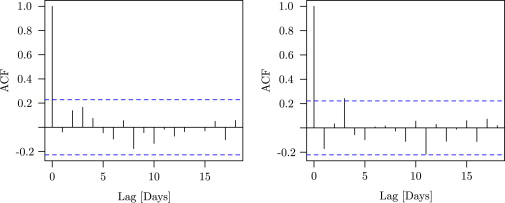
A fundamental assumption of ARMAX models is that the residuals are independent. Therefore, the autocorrelation of the residuals must be checked. Sample autocorrelation functions of the residuals of the model with common gA-values applied on the two data sets are plotted in Figure 8 together with confidence bands for white noise. The estimated autocorrelations are relatively small for both periods, and hence the dynamics of both data sets are well described by the fitted model.

Figure 8. Estimated autocorrelations of the residuals of the fits of Model (23) on the two data periods. Period 1 to the left, period 2 to the right. The dashed blue lines are confidence bands for white noise.

Using this simple ARX model, none of the properties of the building are significantly different between the two periods. It should be noticed that it is difficult to compare model fits on two different data sets. However, it demonstrates consistency in the results using this model. A clear weakness of the model is that averaging to daily values reduces the number of data points dramatically.

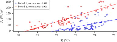
The averaging has another side-effect that may cause problems. Figure 9 shows average solar radiation versus average indoor temperature for the two periods. For period 2, there is a strong correlation (more than 0.9), which means that the impacts of the two are hard to distinguish. An approach to overcome such issues is to excite the system better by varying the indoor temperature independent of other inputs. Section 4.3 introduces methods to avoid this kind of issue in future work.

Figure 9. Average solar radiation versus average indoor air temperature for the two periods. Notice especially for period two, the large correlation between the two.

4. Future work

4.1. Improved measurement and control equipment

In the spring 2011, new measurement equipment and a programmable logic controller (PLC) system were installed in the house. These facilitate online and centralized scheduling and surveillance of experiments. Air temperatures in all rooms, heating and ventilation inlet and outlet temperatures and flows are measured. Moreover open/closed sensors are installed on all exterior doors and windows, and CO₂ concentration is measured in the apartment used for experiments.

A weather station taking meteorological measurements is installed on-site. Ambient temperature and horizontal solar radiation as well as wind speed and direction are measured. An overview of the measurements most relevant to modeling the heat dynamics is provided in Table 5 . Meteorological data is also available from the governmental weather station nearby used for analysis in this paper.

Table 5. The most important measurements in the house for modeling the heat performance of the envelope.

Measurement	Common areas	Rental apartment	Experimental apartment
Indoor temperatures	All rooms	All rooms	All rooms
			Full standard indoor temperature measurement in living room
Heating
Floor heating	2/2	5/5	5/5
Ventilation after heating	All measured together
Ventilation
Central ventilation	All measured together
Outer doors open/closed	2/2	3/3	3/3
Windows open/closed	No windows	2/2	2/2
Cooker hood	0/0	0/1	1/1
Occupancy indicators
PIR sensors	0	0	Living room/kitchen, corridor
CO2 concentration	0	Deactivated	Yes
Consumption
Oil	All measured together
Electricity	1/1	1/1	1/1
PV system	Only one system
Total heat collection
Domestic water heating
Buffer water heating
Heating system	Contributes to common system
Metereological variables	All at one common weather station
Ambient temperature
Solar radiation
Wind speed
Wind direction

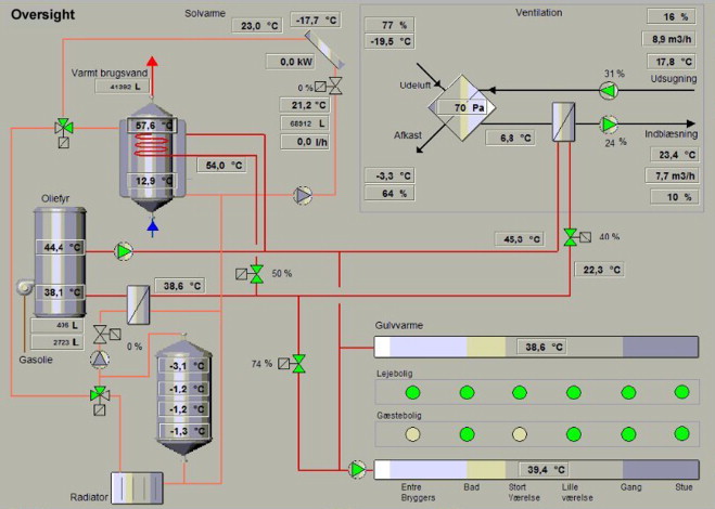
With the new control system, heating and ventilation systems can be controlled based on all measurements, functions hereof, or even exogenous inputs. An overview of the state of the system is available on-line, and a screen dump of this is seen in Figure 10 . The overview intuitively shows how the different systems are connected and interacted. There are two circulation systems, illustrated by different colors of the pipes. Follow the one leading from the boiler; it goes to the domestic hot water tank (if the return valve is open), to ventilation after heating, and/or to floor heating. Before it comes back to the furnace, it passes through a heat exchanger. The other pipe system goes from the solar panel. It goes to either heating the domestic water tank or to the radiator and buffer tank when a surplus of heat from the solar panel is present. The storage tank is both loaded and unloaded from the top so that a vertical temperature gradient can be maintained in the tank.

Figure 10. Overview of the most important flow and temperature measurements in the house.

4.2. Graybox modeling

Formulation and selection of a statistical model is an iterative process, and when modeling systems of high complexity it is often fruitful to start from a simple description and then step-by-step include new terms if they significantly improve the description of the system. An initial description of the heat loss was given in the preceding section. In order to describe the heat dynamics in more detail, graybox models (Madsen and Holst, 1995 ; Andersen et al ., 2000  ;  Bacher and Madsen, 2011 ) can be applied. Graybox modeling combines the advantages of using physical knowledge about the system with statistical methods to obtain precise descriptions of the dynamics behind measurements of a physical system. The stochastic differential equations used are based on the well-known differential equations of heat dynamics which are naturally dynamic. A very simple linear dynamical model of the indoor temperature, ${\textstyle T_{i}}$ , is formulated in (Bacher and Madsen, 2011 ):

$dT_{i}={\frac {1}{C_{h}}}({\frac {T_{a}-T_{i}}{R}}+A_{w}\cdot P_{s}+$$P_{h})dt+{\sigma }_{i}\quad d{\omega }_{i}(t)$

( 24)

where ${\textstyle T_{i}}$ is the indoor temperature, R   is the thermal resistance of the building envelope, ${\textstyle C_{h}}$ is the heat capacity of the building, ${\textstyle A_{w}}$ is the effective area of the windows, and ${\textstyle P_{h}}$ is the heat supply from the heating system. ${\textstyle {\omega }_{i}}$ is a standard Wiener process (a white noise process in continuous time), and ${\textstyle {\sigma }_{i}}$ is a constant. Eq. (24) describes the indoor temperature evolution in continuous time.

Let Y (n ) be the measurement of the indoor temperature at discrete time n :

$Y(n)=T_{i}(n)+\epsilon (n),\quad \epsilon (n)\sim N(0,{\sigma }_{o}^{2})$

( 25)

i.e., the measurements are encumbered with white noise, e (n ). For in-depth treatment of stochastic differential equations, see Øksendal (2007) . For filtering, i.e., re-construction and prediction of the temperature based on measurements, see Jazwinski (2007) .

The test facilities available for the project are expected to enable more detailed observation of the heat dynamics. Hence a more general dynamic heat balance in the house is considered. Let P in general denote a heat flux, and the subscripts h , v , c , s , and i denote the heating system, ventilation, conduction, solar radiation, and infiltration respectively. Then

$dT_{i}={\frac {1}{C_{h}}}(P_{h}+P_{v}+P_{c}+P_{s}+P_{i})\quad dt+{\sigma }_{2}\quad d{\omega }_{2}$

( 26)

expresses the interior temperature development. ${\textstyle {\sigma }_{2}}$ is a constant and ${\textstyle {\omega }_{2}}$ is a standard Wiener process.

The conduction ${\textstyle P_{c}}$ through walls, roof, doors and windows is expected to be of major importance. Let this be an example of how the model can be extended to contain more states, i.e., consist of coupled stochastic differential equations. Let it be given by a conduction from the outside surface temperature of the building, ${\textstyle T_{o}}$ , and the indoor temperature:

$P_{a}={\frac {1}{R_{oi}C_{e}}}(T_{o}-T_{i})$

The outer envelope surface could be cooled (or heated) as modeled by convection. Then that state could be written as follows:

$dT_{o}=({\frac {1}{R_{oi}C_{e}}}(T_{i}-T_{o})+f_{W}(W_{s},W_{d})(T_{a}-$$T_{o}))\quad dt+{\sigma }_{2}d{\omega }_{2}$

( 27)

where f_W could be a non-linear function of wind speed and wind direction. In Jiménez et al. (2008b) with a model similar to this one, f_W is modeled for a PV-module with an allometric function. Further extension in the present case could include dependence on the wind direction.

This non-linear extension of the linear dynamic model is only one of many possible extensions. It has been justified from physical considerations but the main criterion is the ability to describe the behavior of the system, i.e., what is reflected in the data. Hence, standardized model search procedures as in Bacher and Madsen (2011) are needed.

4.3. Experiments in early 2012

Estimation of parameters in graybox modeling requires – depending on the complexity of the models – not only good models, but also good experiments. Parameter estimates can be correlated if parametrization or the experimental plan is sub-optimal. Take Eq. (24) as an example. If ${\textstyle T_{i}}$ is constant, R   and ${\textstyle C_{h}}$ turn out not to be identifiable. Therefore, the indoor temperature has to be varied. For being able to distinguish influences from each other, the input signal (here, the floor heating) must be varied on all frequencies, which can be done using PRBS (Pseudo-Random binary signals) or ROLBS (Randomly Ordered Logarithmically distributed Binary Sequence) signals. The system is said to be excited. This was the focus of experiments that were carried out in 2012. Such input signals are said to be persistently exciting.

5. Conclusions

Statistical modeling of heat dynamics is a strong tool for characterization of and improving energy performance of buildings. A framework of linear dynamic models (ARMAX) was described together with methods to extract important information about heat dynamics from model estimates.

Promising results have already been obtained by applying linear dynamic models on heat dynamics in buildings. An example study was given where 2 periods of 2.5 months each were compared for a described low energy house in Greenland. Repair work was carried out between the two periods, and improved tightness of the envelope was expected in the second period. Heat consumption was modeled using indoor temperature and weather variables, and properties of the building were estimated and compared over the two periods. From the available measurements, the expectation that repair works had made the heating consumption in the building less sensitive to wind could not be demonstrated.

However, long testing time was needed, and separating impacts of different inputs seemed to lead to problems. Test facilities in the Arctic area have been described and the advantages of these in relation to more detailed modeling have been discussed. Finally, some examples on modeling, non-dynamic and dynamic, linear and non-linear have been given. Experiments will be carried out to apply models of this framework on experiments carried out in 2012.

References

1. Andersen et al., 2000 K.K. Andersen, H. Madsen, L.H. Hansen; Modelling the heat dynamics of a building using stochastic differential equations; Energy and Buildings, 31 (1) (2000), pp. 13–24 ISSN 03787788
2. Bacher and Madsen, 2011 P. Bacher, H. Madsen; Identifying suitable models for the heat dynamics of buildings; Energy and Buildings, 43 (2011), pp. 1511–1522 http://doi.org/10.1016/j.enbuild.2011.02.005 ISSN 0378-7788, URL: 〈http://www.sciencedirect.com/science/article/B6V2V-5281SNX-1/2/b2eae0acc59b94e358cc3e7816bd94ae 〉
3. Bacher et al., 2013 Bacher, P., Madsen, H., Nielsen, H.A., Perers, B., 2013. Short-term heat load forecasting for single family houses, Energy and Buildings 65, 101–112, http://dx.doi.org/10.1016/j.enbuild.2013.04.022.
4. Ersbøll and Conradsen, 2005 Ersbøll, B.K., Conradsen, K., 2005. An Introduction to Statistics, 7th ed., vol. 2. Informatics and Mathematical Modelling, Technical University of Denmark, Kongens Lyngby, Denmark.
5. Government of Greenland, 2006 Government of Greenland, Building Regulations 2006, 2006.
6. Jazwinski, 2007 A.H. Jazwinski; Stochastic Processes and Filtering Theory; Courier Dover Publications (2007)
7. Jiménez et al., 2008a M. Jiménez, H. Madsen, K. Andersen; Identification of the main thermal characteristics of building components using MATLAB; Building and Environment, 43 (2) (2008), pp. 170–180 http://doi.org/10.1016/j.buildenv.2006.10.030 URL: 〈http://www.sciencedirect.com/science/article/pii/S0360132306002976 〉, outdoor Testing, Analysis and Modelling of Building Components
8. Jiménez et al., 2008b M. Jiménez, H. Madsen, J. Bloem, B. Dammann; Estimation of non-linear continuous time models for the heat exchange dynamics of building integrated photovoltaic modules; Energy and Buildings, 40 (2) (2008), pp. 157–167 ISSN 03787788
9. Madsen, 2008 H. Madsen; Time Series Analysis; (1st ed.)Chapman & Hall/CRC (2008) ISBN 978-1-4200-5967-0
10. Madsen and Holst, 1995 H. Madsen, J. Holst; Estimation of continuous-time models for the heat dynamics of a building; Energy and Buildings, 22 (1) (1995), pp. 67–79 ISSN 03787788
11. Mortensen and Nielsen, 2010 Mortensen, S., Nielsen, H.A., 2010. Analysis of Energy Consumption in Single Family Houses, Technical Report 03EKS0009A002, Enfor.
12. Norlén, 1990 U. Norlén; Estimating thermal parameters of outdoor test cells; Building and Environment, 25 (1) (1990), pp. 17–24
13. Norling et al., 2006 C.R. Norling, C. Rode, S. Svendsen, J. Kragh, G.P. Reimann; A low-energy building under arctic conditions - a case study; Research in Building Physics and Building Engineering (2006), pp. 587–594
14. Oppenheim et al., 1983 A.V. Oppenheim, A.S. Willsky, S.H. Nawab; Signals and Systems, vol. 2, Prentice-Hall, Englewood Cliffs, NJ (1983)
15. Øksendal, 2007 B. Øksendal; Stochastic Differential Equations; (6th ed.)Springer-Verlag, Berlin Heidelberg (2007) ISBN 3-540-04758-1
16. Rode et al., 2009 Rode, C., Kragh, J., Borchersen, E., Vladyková, P., Furbo, S., Dragsted, J., 2009. Performance of the Low-energy House in Sisimiut. In: Cold Climate HVAC.
17. Tellinghuisen, 2001 J. Tellinghuisen; Statistical error propagation; The Journal of Physical Chemistry A, 105 (15) (2001), pp. 3917–3921
18. Westergren et al., 1999 K.-E. Westergren, H. Högberg, U. Norlén; Monitoring energy consumption in single-family houses; Energy and Buildings, 29 (3) (1999), pp. 247–257