Spare parts supply network optimization with uncertain distributed lead times and demands

Abstract

In the spare parts supply network, there are many uncertain factories, such as unpredictable demands and changeable lead times. The spare parts shortage caused by those uncertainties may lead to severe losses. To solve the uncertainty of supply network, a determined optimization model is developed and then reformulated as a robust counterpart. In the robust model, it is only necessary to know the moment information of the uncertain parameters rather than the true probability distribution. The solution obtained by the robust model can satisfy the constraints in the worst-case, that is, feasible for any probability distribution within the moment based ambiguity set. Two moment based robust models are studied in this work. The result of the experiment indicates that the robustness of the robust model is stronger than that of the determined model and chance constraint model, and the effect of safety tolerance on the robustness is revealed by sensitivity analysis. Finally, the second order moment model is verified to be superior to the first order moment model in spare parts supply network optimization.

Keywords: Spare parts supply network, uncertainty, moment based ambiguity set, chance constraint optimization, distributed robust optimization

1. Introduction

Spare parts supply network optimization is one of the hot issues of spare parts management. Many research works have been done on supply network optimization in certain circumstances. In recent years, many researchers took attention to uncertainty optimization. In the spare parts supply network, many factories such as demands, lead times, and risks are uncertain since the difficulty of data collection or complex dynamic scenarios. Although there are many advanced methods, such as reliability based [1] and data based methods [2], have been used to predict the demands or lead times, most of them are based on over-ideal assumptions and not accurate enough. In fact, in most cases, it almost cannot forecast the demand precisely at all.

To simplify the problems, many researchers assume that the demands are determined [3] or obeys specified known distribution, such as Normal distribution [4], Poisson distribution [5], Stuttering Poisson distribution [6], etc. There are also many works assumed the lead times are fixed [7] or obey known distributions [8]. These assumptions may be not effective sometimes and may cause out of stock or more serious consequences. To handle the uncertainty in the spare parts supply network, most conmen used methods are stochastic program [9], fuzzy optimization [10], and robust optimization [11]. However, in stochastic optimization, it is usually necessary to know the distribution of uncertain parameters in advance or very time-consuming by using Monte Carlo simulation. The fuzzy optimization cannot guarantee the feasibility in all time. Thus, the robust optimization was adopted in this paper because it doesn’t rely on the distribution of uncertain parameters and can guarantee the feasibility of the solution in the worst case.

This paper optimizes the supply network without thus assumption to avoid the serious losses caused by small probability events. The demands and lead times are uncertain with unknown distribution, the only things can we get from the historical data is certain known moments or known structural properties. A moment based ambiguity set was established to descript all the possible distribution, which must contain the real distribution of uncertain parameters. The robust model only needs to ensure the worst case in the ambiguity set is satisfied. The main contributions of this paper are as follows. First of all, the uncertain parameters can obey any distribution with known moments in this paper. Secondly, uncertain demand and lead time are considered at the same time. Thirdly, the robust counterparts are formulated based on inequality theory, which is easily understood than duality theory.

The remaining sections of this article are organized as follows. In Section 2, the determined model of spare parts supply network optimization is developed and then reformulated as its moment based robust counterpart. In section 3, the numerical experiment and sensitivity analysis are carried out. In section 4, the results of the robust model are compared with the determined model and chance constraint model, respectively. Finally, we summarize the paper in section 6.

2. Modeling

The classical three echelon spare parts supply network consists of supply centers, distribution centers and customers. The ordered spare parts are supported by supply centers and then distributed through the distribution centers to meet the spare parts demand of the customers. In the process of supplying, in order to save the costs, it is often unnecessary to open all of the alternative distribution centers. The research aims to decide which distribution center should be opening and also the number of spare parts flow among the nodes of the spare parts supply network.

Different from the traditional supply network, there are many uncertainty parameters in our spare parts supply network. Lead times and demands are the two most conmen considered uncertainty factories in the supply network. In terms of spare parts demands, the predicted values usually do not agree with the real data especially in some complex circumstances. Although, there are lots of state-of-the-art forecast methods are studied and used by researchers, there are still big gaps between the mathematic models and the real-world practice. Similarly, it’s also difficult to ensure the lead times of supply remain unchanged every time, even there may be some accidents that occur in transit. One of the general strategies to handle these uncertainties is assuming these uncertain parameters obey specified distribution. This assumption will not accurate because of the limitation of the historical data. So, in our supply network optimization model, the probability distribution of lead times and demands are even typically unknown. There are only some useful information can be obtained from the samples, such as certain known moments or known structural properties.

The proposed model focus on the problems that optimize the spare parts network with uncertain lead times and demands to meet the customers’ demands within the given hard time window and with the minimum total cost. The uncertainty makes the problem more complicated to be handled. Firstly, the determined model is developed, and then the corresponding robust counterpart problem will be reformulated. The objective function of the model is to minimize the total supply costs, and the constraints of the model include demand fill rate, lead time, captain limitation, flow equilibrium, and so on. The parameters and models are described as follows.

2.1 Parameter description

$I$: the amount of supply centers, $i=1,2,\cdots ,I$;

$J$: the amount of distribution centers, $j=1,2,\cdots ,J$;

$K$: the amount of customers, $k=1,2,\cdots ,K$;

$T_{ij}^{}$: the lead time between supply center $i$ and distribution center $j$ , which is uncertain;

$T_{jk}^{}$: the lead time between distribution center $j$ and customer $k$, which is uncertain;

$T$: the required maximum lead time.

$C_{ij}^{trans}$: unit spare parts transportation costs between supply center $i$ and distribution center $j$;

$C_{jk}^{trans}$: unit spare parts transportation costs between distribution center $j$ and customer $k$;

$C_{j}^{open}$: fixed opening costs of distribution center $j$;

$C_{j}^{invent}$: unit spare parts inventory cost of distribution center $j$;

$C_{k}^{invent}$: unit spare parts inventory cost of customer $k$;

$C_{k}^{short}$ : unit shortage loss of customer $k$;

$d_{k}$: spare parts demand of customer, which is uncertain $k$ ;

$U_{j}$: the maximum spare parts capacity of distribution center $j$ .

Decision variables:

$x_{ij}^{}$ : the amount of spare parts supply from supply center $i$ to distribution center $j$;

$x_{jk}^{}$: the amount of spare parts supply from distribution center $j$ to customer $k$;

$y_{j}^{}$ : binary variable, used to label the opening of distribution center $j$. If distribution center $j$ is opening, $y_{j}^{}=1$, otherwise, $y_{j}^{}=0$.

2.2 Determined model

Firstly, the determined model is developed. In this model, all parameters seem as determined parameters. The objective function is minimizing the total supply costs, which consists of opening cost, transportation costs, inventory costs, and shortage loss. The objective function is formulated as follows:

$\min C=C^{open}+C^{trans}+C^{invent}+C^{short}$

(1)

where $C^{open}$ represents the total opening costs, $C^{trans}$ the total transportation costs, $C^{invent}$ the total inventory costs, and $C^{short}$ the total shortage loss. Each costs are calculated as follows:

$C^{open}=\sum _{j\in J}C_{j}^{open}\cdot y_{j}$

(2)

$C^{trans}=\sum _{i\in I}\sum _{j\in J}C_{ij}^{trans}\cdot x_{ij}+\sum _{j\in J}\sum _{k\in K}C_{jk}^{trans}\cdot x_{jk}$

(3)

$C^{invent}=\sum _{j\in J}C_{j}^{invent}\cdot \left(\sum _{i\in I}x_{ij}-\sum _{k\in K}x_{jk}\right)+\sum _{k\in K}C_{k}^{invent}\Xi \cdot \left(\sum _{j\in J}x_{jk}-d_{k}\right)$

(4)

$C^{short}=\sum _{k\in K}C_{k}^{short}\cdot \Xi \cdot \left(d_{k}-\sum _{j\in J}x_{jk}\right)$

(5)

where $\Xi \lbrace .\rbrace$ represents $max(0,.)$ .

The following constraints should be satisfied:

s.t.

$\sum _{i\in I}\sum _{j\in J}T_{ij}\cdot sgn\left(x_{ij}\right)+\sum _{j\in J}\sum _{k\in K}T_{jk}\cdot sgn\left(x_{jk}\right)-T\leq 0$

(6)

$\sum _{i\in I}x_{ij}-y_{j}\cdot U_{j}\leq 0,\qquad j=1,2,\cdots ,J$

(7)

$\sum _{k\in K}x_{jk}-y_{j}\cdot U_{j}\leq 0,\qquad j=1,2,\cdots ,J$

(8)

$d_{k}-\sum _{j\in J}x_{jk}\leq 0,\qquad k=1,2,\cdots ,K$

(9)

$\sum _{k\in K}x_{jk}-\sum _{i\in I}x_{ij}\leq 0,\qquad j=1,2,\cdots ,J$

(10)

${\begin{array}{c}x_{ij}\in N^{+}\\x_{jk}\in N^{+}\\y_{j}=\left\{0,1\right\}\end{array}}$

(11)

where, constraint (6) is a hard time window constraint, which specifies that the spare parts must arrive at the customers before the deadline. The constraints (7) and (8) state that the closed distribution centers should not participate in the supply of spare parts. They also specify that the input of spare parts should not exceed the maximum capacity of distribution centers. Constraint (9) specifies that the demands of spare parts of all the customers must be satisfied. Constraint (10) ensures that the output of spare parts should not exceed the spare parts flow into each distribution center. Constraint (11) states the character of decision variables.

2.3 Robust counterpart problem reformulation

In the determined supply optimization model, there will be two situations of spare parts shortage. One of them is the spare parts cannot arrive in time, and another is the amount of supplied spare parts cannot meet the demand of customers. Both the two kinds of shortage can lead to serious consequences. In the determined model, it is only necessary to find the feasible solutions that satisfy all the constraints of the model. However, in the uncertain model, it is hard to find feasible solutions because of the uncertainty of lead times and demands. We need to reformulate the mathematical model in the uncertain environment and find robust solutions to ensure that the demands of spare parts are satisfied in any case. This section reformulates the determined model as an uncertain model and derives a tractable and efficient deterministic robust counterpart for the uncertain model.

For most supply practices, the supply environment is complex and changeable, and the sample data is limited. It is usually difficult to get the true probability distribution of these parameters. What only can we do is that extract useful information from these limited samples and use the statistical features to modeling and analysis. Despite the unknown distribution of parameters, the moment, such as, mean, variance, covariances, etc., can be obtained easily. The known moment of the sample contains a lot of valuable information about the distribution, so we use a moment-based ambiguity sets describe the uncertain parameters. This ambiguity set consists of all possible probability distributions satisfied the moment condition, and deservedly contains the true distribution of our parameters. If we can find the robust solutions that satisfy the constraints in the worst-case, then the constraints with real distribution can also be met by the robust solutions.

This section focuses on the robust counterpart reformulation in the case of known first order moments and the case of known both the first order and the second order moments. The ambiguity set of these two cases are expressed as follows, respectively:

$D=\left\{f(\xi ):{\begin{array}{c}\displaystyle {\int }_{\xi \in R^{K}}f(\xi )d\xi =1\\E[\xi ]-{\mu }_{0}=0\end{array}}\right\}$

(12)

$D=\left\{f(\xi ):{\begin{array}{c}\displaystyle {\int }_{\xi \in R^{K}}f(\xi )d\xi =1\\E[\xi ]-{\mu }_{0}=0\\var(\xi )=E[{\left(\xi -{\mu }_{0}\right)}^{2}]={\sigma }_{0}^{2}\end{array}}\right\}$

(13)

where, Eqs. (12) is the ambiguity set with known first order moment, and Eqs. (13) is the ambiguity set with the known first and second order moment. The parameter ${\mu }_{0}$ and ${\sigma }_{0}^{2}$ represent the mean and variance obtained from historical data, $D$ denotes the support of the family of all probability distributions with known moment information and $f(\xi )$ is the probability density function (PDF) of the random variable $\xi$.

If the function objective consists uncertain parameters, it can be use the expectation of objective to reformulate, or transfer the objective function to constraints [12]. In our spare parts optimization model, the uncertain parameters just exist in constraints. In Eqs. (6) and (9), the lead time $T_{ij}$ and $T_{jk}$ and the spare parts demands $d_{k}$ are uncertainty with some unknown distribution. It can be formulate as chance constraints to ensure that the constraint must be satisfied under a probability which greater than the specified threshold.

The single chance constraint of Eqs. (6) is as follows:

$Pr(\sum _{i\in I}\sum _{j\in J}T_{ij}\cdot sgn(x_{ij})+\sum _{j\in J}\sum _{k\in K}T_{jk}\cdot sgn(x_{jk})-T\leq 0)\geq 1-\epsilon$

(14)

The single chance constraint of Eqs. (9) is as follows:

$Pr(d_{k}-\sum _{j\in J}x_{jk}\leq 0)\geq 1-\epsilon ,\qquad k=1,2,\cdots ,K$

(15)

where, $\epsilon \in (0,1)$ represents a specified safety tolerance or violation probability, and all constraints take the same $\epsilon$.

In terms of random variable $\xi$, if the probability density function $\xi$ is known, it is easy to solve the inequality $Pr(\xi \leq b)\leq \alpha$ by $b\leq F_{\xi }^{-1}(\alpha )$ [13]. However, in our spare parts network, the distribution of lead times and demands are unknown. Even the PDF of the lead times is known, it still be difficult and time-consuming to calculate the PDF of $\sum _{i\in I}\sum _{j\in J}T_{ij}\cdot sgn(x_{ij})+$$\sum _{j\in J}\sum _{k\in K}T_{jk}\cdot sgn(x_{jk})$. Therefore, further derivation of Eqs. (14) and Eqs. (15) is needed. We use the robust chance constraints to formulate inequality (14) and (15) as follows:

${\underset {P\in D_{T}}{inf}}Pr(\sum _{i\in I}\sum _{j\in J}T_{ij}\cdot sgn(x_{ij})+\sum _{j\in J}\sum _{k\in K}T_{jk}\cdot sgn(x_{jk})-T\leq 0)\geq 1-\epsilon$

(16)

${\underset {P\in D_{d}}{inf}}Pr(d_{k}-\sum _{j\in J}x_{jk}\leq 0)\geq 1-\epsilon ,\qquad k=1,2,\cdots ,K$

(17)

In the case of only the first order moments are known, for an arbitrary distributional random variable ${\mbox{ }}{\mbox{ }}{\mbox{ }}\xi$. According to the Markov's inequality, there is $Pr\left\{\xi \geq k\right\}\leq {\frac {E(\xi )}{k}},\,X\geq 0,k\geq 0$. Therefore, we can get the robust counterparts of Eqs. (16) and (17) as follows:

$E\left\{\sum _{i\in I}\sum _{j\in J}T_{ij}\cdot sgn(x_{ij})+\sum _{j\in J}\sum _{k\in K}T_{jk}\cdot sgn(x_{jk})\right\}\leq T\epsilon$

(18)

${\frac {E(d_{k})}{\sum _{j\in J}x_{jk}}}\leq \epsilon ,\qquad k=1,2,\cdots ,K$

(19)

Proof. For inequality (16), there is:

${\underset {P\in D_{T}}{inf}}Pr\left(\sum _{i\in I}\sum _{j\in J}T_{ij}\cdot sgn(x_{ij})+\sum _{j\in J}\sum _{k\in K}T_{jk}\cdot sgn(x_{jk})-T\leq 0\right)$ $={\underset {P\in D_{T}}{inf}}\left\{1-Pr(\sum _{i\in I}\sum _{j\in J}T_{ij}\cdot sgn(x_{ij})+\sum _{j\in J}\sum _{k\in K}T_{jk}\cdot sgn(x_{jk})\geq T\right\}$ $\geq 1-{\frac {E\left\{\sum _{i\in I}\sum _{j\in J}T_{ij}\cdot sgn(x_{ij})+\sum _{j\in J}\sum _{k\in K}T_{jk}\cdot sgn(x_{jk})\right\}}{T}}\geq 1-\epsilon$ $\Rightarrow E\left\{\sum _{i\in I}\sum _{j\in J}T_{ij}\cdot sgn(x_{ij})+\sum _{j\in J}\sum _{k\in K}T_{jk}\cdot sgn(x_{jk})\right\}\leq T\epsilon$

For inequality (17), there is:

${\underset {P\in D_{d}}{inf}}Pr(d_{k}-\sum _{j\in J}x_{jk}^{}\leq 0)=1-{\underset {P\in D_{d}}{sup}}Pr(d_{k}-\sum _{j\in J}x_{jk}\geq 0)$ $\geq 1-{\frac {E(d_{k})}{\sum _{j\in J}x_{jk}}}\geq 1-\epsilon$ $\Rightarrow {\frac {E(d_{k})}{\sum _{j\in J}x_{jk}}}\leq \epsilon$

In the case of both the first and second order moments are known, for an arbitrary distributional random variable $\xi$. According to the Cantelli's inequality, there is, $Pr\left\{\xi -\mu \geq k\right\}\leq {\frac {{\sigma }^{2}}{{\sigma }^{2}+k^{2}}},$ $k\geq 0$. Therefore, we can get the robust counterparts of constraint (16) and (17) as follows:

$\displaystyle {\frac {var\left\{\displaystyle \sum _{i\in I}\sum _{j\in J}T_{ij}\cdot sgn(x_{ij}^{})+\displaystyle \sum _{j\in J}\displaystyle \sum _{k\in K}T_{jk}\cdot sgn(x_{jk})\right\}}{var\left\{\displaystyle \sum _{i\in I}\displaystyle \sum _{j\in J}T_{ij}\cdot sgn(x_{ij})+\displaystyle \sum _{j\in J}\displaystyle \sum _{k\in K}T_{jk}\cdot sgn(x_{jk})\right\}+(E\left\{\displaystyle \sum _{i\in I}\displaystyle \sum _{j\in J}T_{ij}\cdot sgn(x_{ij})+\displaystyle \sum _{j\in J}\displaystyle \sum _{k\in K}T_{jk}\cdot sgn(x_{jk})\right\}-T)^{2}}}\leq \varepsilon$ (20)

${\frac {var(d_{k})}{var(d_{k})+{\left(\displaystyle \sum _{j\in J}x_{jk}-E(d_{k})\right)}^{2}}}\leq \epsilon ,\qquad k=1,2,\cdots ,K$

(21)

Proof. For inequality (16), there is:

${\underset {P\in D_{T}}{inf}}Pr\left(\sum _{i\in I}\sum _{j\in J}T_{ij}\cdot sgn(x_{ij})+\sum _{j\in J}\sum _{k\in K}T_{jk}\cdot sgn(x_{jk})-T\right)\leq 0$ $={\underset {P\in D_{T}}{inf}}\left\{1-Pr\left(\sum _{i\in I}\sum _{j\in J}T_{ij}\cdot sgn(x_{ij})+\sum _{j\in J}\sum _{k\in K}T_{jk}\cdot sgn(x_{jk})\geq T\right)\right\}\geq 1$ $-{\frac {var\left\{\displaystyle \sum _{i\in I}\sum _{j\in J}T_{ij}^{\cdot }sgn(x_{ij})+\displaystyle \sum _{j\in J}\displaystyle \sum _{k\in K}T_{jk}\cdot sgn(x_{jk})\right\}}{var\left\{\displaystyle \sum _{i\in I}\displaystyle \sum _{j\in J}T_{ij}\cdot sgn(x_{ij})+\displaystyle \sum _{j\in J}\displaystyle \sum _{k\in K}T_{jk}\cdot sgn(x_{jk})\right\}+{\left(E\left\{\displaystyle \sum _{i\in I}\displaystyle \sum _{j\in J}T_{ij}\cdot sgn(x_{ij})+\displaystyle \sum _{j\in J}\displaystyle \sum _{k\in K}T_{jk}\cdot sgn(x_{jk})\right\}-T\right)}^{2}}}\geq 1-\epsilon$ $\Rightarrow \displaystyle {\frac {var\left\{\displaystyle \sum _{i\in I}\displaystyle \sum _{j\in J}T_{ij}^{}\cdot sgn(x_{ij}^{})+\displaystyle \sum _{j\in J}\sum _{k\in K}T_{jk}^{}\cdot sgn(x_{jk}^{})\right\}}{var\left\{\displaystyle \sum _{i\in I}\displaystyle \sum _{j\in J}T_{ij}^{}\cdot sgn(x_{ij}^{})+\displaystyle \sum _{j\in J}\displaystyle \sum _{k\in K}T_{jk}^{}\cdot sgn(x_{jk}^{})\right\}+(E\left\{\displaystyle \sum _{i\in I}\displaystyle \sum _{j\in J}T_{ij}^{}\cdot sgn(x_{ij}^{})+\displaystyle \sum _{j\in J}\displaystyle \sum _{k\in K}T_{jk}^{}\cdot sgn(x_{jk}^{})\right\}-T)^{2}}}\leq \varepsilon$

For inequality (17), there is:

${\mbox{ }}{\underset {P\in D_{d}}{inf}}Pr(d_{k}-\sum _{j\in J}x_{jk}^{}\leq 0{\mbox{ }})=1-{\underset {P\in D_{d}}{sup}}Pr(d_{k}-\sum _{j\in J}x_{jk}^{}\geq 0{\mbox{ }})$ $\geq {\mbox{ }}1-{\frac {var(d_{k})}{var(d_{k})+{\left(\sum _{j\in J}x_{jk}^{}-E(d_{k})\right)}^{2}}}\geq 1-\epsilon$ $\Rightarrow {\frac {var(d_{k})}{var(d_{k})+{\left(\sum _{j\in J}x_{jk}^{}-E(d_{k})\right)}^{2}}}\leq \epsilon$

In summary, the robust counterpart is derivated by replace the inequality (6) and (9) of the determined model by the inequality (18) and (19) or inequality (20) and (21).

3. Case study

3.1 Case description

In this case, the three echelon spare parts supply network consists of 2 supply centers, 5 distribution centers, and 4 customers. The spare parts are supported to meet the demands of customers. The first and second moments of the lead times and demands are counted from 50 samples. The relative data are shown in Tables 1-4. The required maximum lead time is 300 hours, and the safety tolerance $\epsilon$ is set from 0.1 to 0.9, respectively. The problems were solved by CPLEX and differential evolutionary algorithm.

3.2 Results and sensitive analysis

The optimal solutions of the robust optimization model with known first order moment (referred to as the first order moment model) and with known first and second moment (referred to as the second order moment model) are obtained, their corresponding objective functions and constraints are also calculated and shown in Table 5. In order to analyze the effect of safety tolerance $\epsilon$ on the robustness of the model, we take multiple values of $\epsilon$ in the first order moment model and the second order moment model, respectively. Constraint 1-20 in Table 5 is the value of the left side of the corresponding inequality constraints, that is, if the value is big than zero, the corresponding constraints are violated, otherwise, the constraint is satisfied. The following conclusion can be summed from the table:

(1) As the safety tolerance increases, the robustness of the model is gradually slack. In other words, the smaller the safety tolerance, the stricter the robustness of the constraints is. In the first order moment model, the feasible solution is obtained only when the tolerance is set as 0.9, and the constraint value is greater than zero in other cases (bold in the table), which indicates unfeasible. Comparing the value of these unfeasible solutions, it can be found that the increase of safety tolerance leads to a decrease of constraint violation degree.

Table 1. The opening costs, inventory costs and inventory capacity of distribution centers

	Distribution centers 1	Distribution centers 2	Distribution centers 3	Distribution centers 4	Distribution centers 5
Opening costs	1000	1500	2500	1800	2000
Inventory costs	12	8<	5	10	10
Inventory capacity	50	55	80	60	65

Table 2. The shortage loss, inventory costs, and demands of customers

	customer1	customer2	customer3	customer4
Shortage loss	100	120	80	150
Inventory costs	10	15	12
Expectation of demands	68	61	57	88
Variance of demands	9<	11<	7</	8

Table 3. The transportation costs between nodes of supply network

	Distribution centers 1	Distribution centers 2	Distribution centers 3	Distribution centers 4	Distribution centers 5
Supply center1	105	104	102	104	110
Supply center2	94	108	105	98	96
Customer 1	46	42	59	54	46
Customer 2	41	67	61	67	41
Customer 3	49	53	51	49	49
Customer 4	55	49	60	51	55

Table 4. The lead times between nodes of the supply network

	Distribution centers 1	Distribution centers 2	Distribution centers 3	Distribution centers 4	Distribution centers 5
Supply center1	12/1.6	11/2.5	9/1.8	11/1.1	10/2.3
Supply center2	7/0.7	15/1.3	15/1.6	7.5/1.8	8/1.1
Customer 1	5/0.2	5/0.3	7/0.5	3.7/1.2	4/0.8
Customer 2	4/0.8	5/1.1	3/0.2	4.5/0.6	4/0.3
Customer 3	3.5/0.3	2.5/0.3	2.9/0.7	1.5/0.4	5/0.8
Customer 4	2.6/0.2	4/0.4	1.6/0.2	2/0.5	3.5/0.7

(2) The value of the objective function decreases gradually as the robustness of the model enhanced. This is because when the robustness is very strict, the solutions try to meet the constraints as much as possible for the price of at the expense of objective function. For example, in order to meet the demand constraint, decision makers have to increase the amount of supplied spare parts, which makes the transportation and inventory costs increase greatly. Therefore, it’s necessary to judge and weigh the smaller objective function and the higher robust constraints to find a balance point.

(3) The robustness of the first order moment model is stronger than that of the second order moment model. However, the robustness of the first order moment model is too strict, and the feasible solutions may not be able to be found. That is because when using the Markov's inequality, the probability of constraints satisfied is reduced too small, and a lot of information is missed during this process. However, the second-order moment model is not as strict as the first-order moment model, because there is more distribution information in the second order moment. In the actual spare parts supply, if the robustness is emphasized too much, the feasibility of the solution cannot be guaranteed, and the cost of supply will be increased at the same time. It can see that, the result of second order moment model is better than the first order moment model.

Table 5. Objective function and constraints of first order and second-order moment model

Model	First order moment model					Second order moment model
Safety tolerance	0.1	0.3	0.5	0.7	0.9	0.1	0.3	0.5	0.7	0.9
Costs	42029	41679	41168	40958	39480	42634	41172	41120	39459	39392
Constraint 1	130.3	86.3	23.3	-30.2	-199.8	-1421.134	-5796.052	-10530.2	-10105.74	-13000.61
2	0	0	0	0	0	0	-3	-2	-6	-5
3	0	-1	0	0	-4	0	-1	0	-2	0
4	0	0	0	0	0	-4	-1	-5	0	-1
5	0	0	0	0	0	-1	0	0	-2	-2
6	-1	-11	0	0	0	-3	-4	-2	-6	-6
7	-2	-2	-1	0	0	0	-5	-9	-7	-6
8	-1	-5	-4	-1	-4	-6	-4	0	-2	0
9	0	-1	-2	-1	0	-4	-2	-5	0	-2
10	-2	0	0	0	0	-8	0	-1	-3	-2
11	-7	-11	-1	0	0	-7	-5	-6	-6	-6
12	59.2	41.6	26.5	15.5	-0.4	-17.5	-126	-195.5	-82	-56.7
13	55.4	44.5	31	16.2	-0.2	-2.2	-3.1	-7	-3	-2.5
14	51.8	44.4	26.5	19.2	-0.6	-0.1	-5.9	-9	-0.7	-2.9
15	77.8	56.2	39	7.5	-0.2	-12.4	-30.7	-8.5	-98.4	-128.8
16	-2	-2	-1	0	0	0	-2	-7	-1	-1
17	-1	-4	-4	-1	0	-6	-3	0	0	0
18	0	-1	-2	-1	0	0	-1	0	0	-1
19	-2	0	0	0	0	-7	0	-1	-1	0
20	-6	0	-1	0	0	-4	-1	-4	0	0

4. Robustness analysis

To verify the robustness of the uncertain model, we compare the results of the robust model with the determined model and the opportunity constraint model, respectively. Robust model refers to the first or second order moment model. The determined model refers to the model with the expected value of the uncertain parameter, which is adopted by most decision makers. The chance constraint model refers to the model with the assumption that the distribution of uncertain parameters is known. Because the distribution is unknown, the Monte Carlo method is used to solve the chance constraint model.

4.1 Comparison with determined model

In the determined model developed in section 2.3 of this paper, the expectation of lead times时and spare parts demands are adopted as the determined parameters. The comparison with the determined model is taken from two aspects. In the first aspect, the solutions of the first order moment model and the second order moment model (referred to as the robust solution) are brought into the deterministic model to test the feasibility of the robust solution in the determined model.

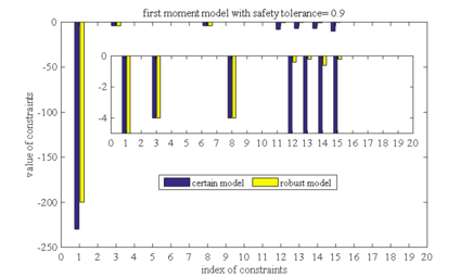
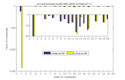
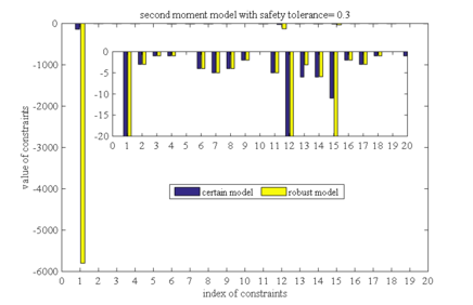
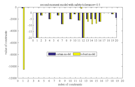
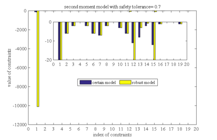
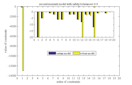
Brought the robust solutions under different safety tolerances into the determined models, and the values of all constraints are calculated respectively. The constraint value indicates constraint violation, and if the constraint value is less than or equal to 0, it means that the constraint is satisfied. Figure 1-10 is the histograms of the constraints values in these ten different cases, respectively (two different order moment models with five safety tolerance). Figure 1, taken as an example, shows the constraints values that bring the robust solutions of the first order moment model with a safety tolerance of 0.1 into the determined model. The horizontal axis represents the index of the constraint, and there are a total of 20 constraints in our case. The vertical axis is a constraint value, the yellow bars (labeled as robust model) are the constraint values of the robust model, and the blue bars (labeled as certain model) are the constraint values of determined the model.

In Figure 1, the constraints 1,12,13,14 and 15 of the robust model are not satisfied. In the corresponding determination model, there are only two violated constraints, that is, constraint 13 and constraint 14. It can be seen that although the robust solution is still unfeasible in the deterministic model, it greatly reduces the constraints violate degree. It can be seen that the first order moment model has good robustness, and the same conclusion can be drawn from Figures 2 to Figure 10.

Comparing the results in Figures 1 to Figure 5 (or Figures 6 to Figure 10), it can also be found that the constraint violations of both the determined model and the robust model decrease as the safety tolerance increases, which is consistent with conclusion (2) in section 5.2. Comparing the results of first order moment model with those in second order moment model, we can find that the robust solution of the second-order moment model makes the constraint violations in determined model much smaller than the robust solution of the first-order moment model. This conclusion is consistent with conclusion (3) in section 5.2.

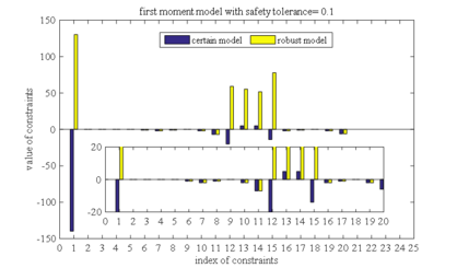
Figure 1. Constraint violation comparison between first order moment model and determined model as safety tolerance is 0.1

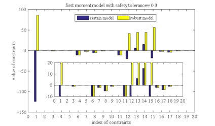
Figure 2. Constraint violation comparison between first order moment model and determined model as safety tolerance is 0.3

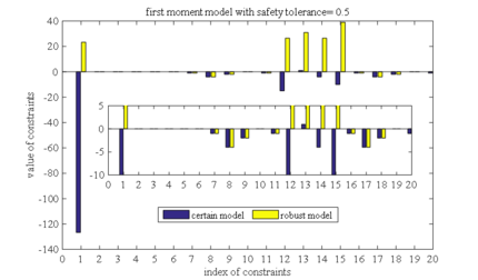
Figure 3. Constraint violation comparison between first order moment model and determined model as safety tolerance is 0.5

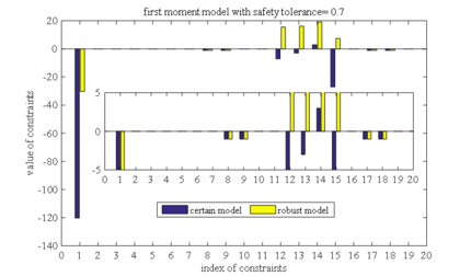
Figure 4. Constraint violation comparison between first order moment model and determined model as safety tolerance is 0.7

Figure 5. Constraint violation comparison between first order moment model and determined model as safety tolerance is 0.9

Figure 6. Constraint violation comparison between second order moment model and determined model as safety tolerance is 0.1

Figure 7. Constraint violation comparison between second order moment model and determined model as safety tolerance is 0.3

Figure 8. Constraint violation comparison between second order moment model and determined model as safety tolerance is 0.5

Figure 9. Constraint violation comparison between second order moment model and determined model as safety tolerance is 0.7

Figure 10. Constraint violation comparison between second order moment model and determined model as safety tolerance is 0.9

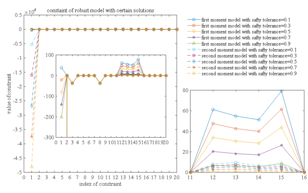
In the second aspect, take the feasible solutions obtained from the determined model into robust models to test the feasibility of the determined solutions in the robust model, and the results are shown in Figure 11. It can be seen from the figure that all the determined solutions are infeasible in the robust model. The results indicate that the solutions of the determined model can only guarantee the feasibility in a specific case, but not in the models with uncertain distribution parameters. Generally, the constraints violation degree in the second order moment model is significantly smaller than that in the first order moment model, which indicates that the first order moment is stricter than the second order moment model. With the increase of safety tolerance, the constraint violation degree decreases gradually, which indicates that the smaller the safety tolerance, the more strict of the robustness of the model is.

Figure 11. Constraint violation comparison between robust model and chance constraint model

4.2 Comparison with chance constraint model

In this section, the feasibility of robust solutions in the chance constraint model is verified. Take the robust solutions of first order moment model and second order moment model into the chance constraint model to test the feasibility. Since the uncertain parameters only exist in the constraints (6) and (9) of the spare parts supply model, only these two inequality constraints need to be tested. The corresponding opportunity constraint models are:

$Pr\left(\sum _{i\in I}\sum _{j\in J}T_{ij}\cdot sgn(x_{ij})+\sum _{j\in J}\sum _{k\in K}T_{jk}\cdot sgn(x_{jk})\leq T\right)\geq 1-\epsilon$

(22)

$Pr\left(d_{k}-\sum _{j\in J}x_{jk}\leq 0\right)\geq 1-\epsilon ,\qquad k=1,2,\cdots ,K$

(23)

Since unknown the probability distribution of lead times and demands, it cannot be solved by probability density function. Even if the distribution of uncertain parameters is known, the solution of the joint probability density function in Equation (23) is very time-consuming. So the Monte Carlo method is used to verify the feasibility of the solution

Because the first order moment robust optimization model is not feasible, only the second order moment optimization model is compared and analyzed.

50 samples of uncertain parameters are selected, take the robust solution of the second-order moment model into these samples, and calculate the times $N_{T}'$ and $N_{d}'$ that inequalities (22) and (23) are satisfied

$N_{T}'=\sum _{n=1}^{N}\Delta \left(\sum _{i\in I}\sum _{j\in J}T_{ij}\cdot sgn(x_{ij})+\sum _{j\in J}\sum _{k\in K}T_{jk}\cdot sgn(x_{jk})\leq T\right)$

(24)

$N_{d}'=\sum _{n=1}^{N}\Delta \left(d_{k}-\sum _{j\in J}x_{jk}\leq 0\right)$

(25)

where, $\Delta (.)=1$, if $.$ is satisfied. else if, $\Delta (.)=0$. Then, $N_{T}{}'/N$ and $N_{d}'/N$ are used to represent the value of $Pr(\sum _{i\in I}\sum _{j\in J}T_{ij}\cdot sgn(x_{ij})+$$\sum _{j\in J}\sum _{k\in K}T_{jk}\cdot sgn(x_{jk})\leq T)$ and $Pr(d_{k}-\sum _{j\in J}x_{jk}\leq 0)$. If $N_{T}'/N$ or $N_{d}'/N$ were greater than or equal to $1-\epsilon$, the constraints (22) and (23) are satisfied.

The constraint satisfactions of the chance constraint model are shown in Table 6. It can be seen that the constraints (22) and (23) are satisfied in all scenarios. As the safety tolerance decrease, the value of $N_{T}'/N$ and $N_{d}'/N$ are larger. This is because when the safety tolerance is small, the robust model is more strict, and the robustness of the robust solution is stronger, which lead to the greater the probability that the constraint is satisfied in chance constraint model.

Table 6. The constraint satisfied probability with second order moment model robust solution

$\epsilon$	0.1	0.3	0.5	0.7	0.9
$N_{T}'/N$	0.9692	0.8997	0.7938	0.7288	0.6992
$N_{d}'/N$, $k=1$	0.9269	0.8194	0.8187	0.7938	0.7994
$N_{d}'/N$, $k=2$	0.9524	0.8219	0.8170	0.7922	0.7223
$N_{d}'/N$, $k=3$	0.9461	0.9403	0.9396	0.8959	0.8843
$N_{d}'/N$, $k=4$	0.9289	0.8351	0.7378	0.7298	0.6537

5. Conclusion

In this paper, the spare parts network optimization with uncertainty lead times and demands is studied. The determined supply model and its robust counterpart are developed, respectively. In the uncertainty model, the probability of the uncertainties are unknown, we focus on the reformulation of this model with the known first and second order moment. The robust solutions of uncertain models are obtained and the sensitivity analysis with different safety tolerance is curry out. Then the robustness is compared between the robust model and determined model and chance constraint model. The main contributions of this paper are as follows. Firstly, the ambiguity set is used to handle the uncertain probability distributions, and the robust counterpart of the supply model is reformulated to make the model tractable and computable. Secondly, the robust solutions that ensure the feasibility in the worst-case are obtained. These solutions ensure that the uncertain constraints are satisfied under any probability distribution within the moment based ambiguity set. The results of the case study show that the robustness of these solutions are stronger than those in the determined model and chance constraint model. Finally, we verified that the second order moment model is superior to the first moment order model because the second order moment model can make a balance in robustness and flexibility.

References

[1] Eaves A.H.C.，Kingsman B.G. Forecasting for the ordering and stock-holding of spare parts. Journal of the Operational Research Society, 55(4):431-437, 2004.

[2] Mao H.L., Gao J.W., Chen X.J., Gao J.D. Demand prediction of the rarely used spare parts based on the BP neural network. Applied Mechanics and Materials, 519-520:1513–1519, 2014.

[3] Sadeghi J., Sadeghi S., Niaki S.T.A. (2014). A hybrid vendor managed inventory and redundancy allocation optimization problem in supply chain management: An NSGA-II with tuned parameters. Computers & Operations Research, 41:53–64, 2014.

[4] Qiu Z., Ni Z. Probabilistic interval approach for determining the demand of aviation spares. Acta Aeronautica Et Astronautica Sinica, 30(5):861-866, 2004.

[5] Axsäter S. Optimization of order-up-to-s policies in two-echelon inventory systems with periodic review. Naval Research Logistics, 40(2):245–253, 1993.

[6] Kouki C., Babai M.Z., Jemai Z., Minner S. Solution procedures for lost sales base-stock inventory systems with compound poisson demand. International Journal of Production Economics, S0925527318300513, 2018.

[7] Al-Rifai M.H., Rossetti M.D. An efficient heuristic optimization algorithm for a two-echelon (R, Q) inventory system. International Journal of Production Economics, 109(1-2):195–213, 2007.

[8] Hnaien F., Delorme X., Dolgui A. Multi-objective optimization for inventory control in two-level assembly systems under uncertainty of lead times. Computers & Operations Research, 37(11):1835–1843, 2010.

[9] Gicquel C., Cheng J. A joint chance-constrained programming approach for the single-item capacitated lot-sizing problem with stochastic demand. Annals of Operations Research, 264(1-2):123-155, 2018.

[10] Talaei M., Farhang M.B., Pishvaee M.S., et.al. A robust fuzzy optimization model for carbon-efficient closed-loop supply chain network design problem: a numerical illustration in electronics industry. Journal of Cleaner Production, 113:662–673, 2016.

[11] Shang C., You F. Distributionally robust optimization for planning and scheduling under uncertainty. Computers & Chemical Engineering, 110(FEB.2):53-68, 2018.

[12] Shi Y., Boudouh T., Grunder O. A fuzzy chance-constraint programming model for a home health care routing problem with fuzzy demand. International Conference on Operations Research & Enterprise Systems, 2017.

[13] Rubinstein R.Y, Kroese D.P. Simulation and the Monte Carlo method by Reuven Y. Rubinstein. Journal of the American Statistical Association, 78(382):511-512 1983.

---

• Corresponding author. Tel.: +86 18795428481; E-mail: xwzj0003@gmail.com