Machine learning techniques to predict the compressive strength of concrete

Abstract

Conventional concrete is the most common material used in civil construction and its behavior is highly nonlinear, mainly because of its heterogeneous characteristics. Compressive strength is one of the most critical parameters when designing concrete structures and it is widely used by engineers. This parameter is usually determined through expensive laboratory tests, causing a loss of resources, materials and time. However, artificial intelligence and its numerous applications are examples of new technologies that have been used successfully in scientific applications. Artificial Neural Network (ANN) and Support Vector Machine (SVM) models are generally used to resolve engineering problems. In this work, three models are designed, implemented and tested to determine the compressive strength of concrete: Random Forest, SVM and ANN. Pre-processing data, statistical methods and data visualization techniques are also employed to gain a better understanding of the database. Finally, the results obtained show high efficiency and are compared with other works, which also captured the compressive strength of the concrete.

Keywords: Compressive strength of concrete, artificial neural network, support vector machine, random forest

1. Introduction

Conventional concrete is the most common material used in civil construction, being a mixture composed of water, cement and different aggregates. Its resistance mainly depends on factors such as cement consumption, water-cement factor, degree of condensation and the nature of aggregates. The compressive strength of concrete is quite considerable, but its tensile strength is much lower. Owing to this, the concrete can be classified as a fragile material, having entirely different strength properties under tensile and compression tests [1].

The compressive strength of concrete is still one of the most widely used parameters in structural engineering for the design of reinforced concrete structures. The performance of concrete, when defined empirically, can be affected by nonlinear factors, when using the concrete compression test as a destructive procedure on concrete specimens. However, this activity involves time, planning and financial resources because the commonly used compressive strength factor is obtained on the 28th day [2].

Technological advancement allows engineering problems to be solved by the use of machine learning methods and their applications can represent good examples of fields explored with different expectations and realistic results. In general, artificial intelligence systems have shown their ability to solve real-life problems, particularly in nonlinear tasks [3]. Structural engineering has been a field of significant development through the implementation and testing of new computational models, that are able to predict the different properties of concrete mixtures. In the case of behavioral models, pattern recognition is constructive and computational intelligence methods can be used. Bio-inspired models can also be an excellent aid to the design of structures for civil engineering [4–8]. With the development of artificial intelligence, it is easier to forecast concrete compressive strength. When compared with other traditional regression methods, machine learning adopts specific algorithms that can learn from the input data and gives highly accurate results.

Currently, several machine learning algorithms are used for concrete compressive strength prediction, among which are Random Forest, Artificial Neural Network and Support Vector Machine models. A brief review on the subject is given below.

Recently, Feng et al. [9] used a new technique called XGBoosting to predict the concrete compressive strength with good results. They also used ANN and SVM to compare the obtained results with excellent predictions. ANN and Adaptive Neuro-Fuzzy Inference System (ANFIS) models were used to predict a cement-based mortar material compressive strength [10]. The paper demonstrates the ability of ANN and ANFIS models to approximate the compressive strength of mortars reliably and robustly. Also, ANN were applied to predict the strength of concrete containing construction waste, recycled aggregate concrete [11] and self-compacting concrete containing bottom ash [12]. ANN were used again to predict the strength of environmentally friendly concrete [13]. They showed that ANN models can provide high-performance prediction for concrete compressive strength. The application of ANN in predicting the compressive strength of concrete containing nano-silica and copper slag was also addressed by Chithra et al. [14], showing promising results. Machine learning techniques such as ANN and SVM were used [15] and least-square SVM was improved using the metaheuristic optimization to predict the compressive strength of high-performance concrete [16]. The compared accuracy of different data mining techniques was applied for predicting the compressive strength of environmentally friendly concrete [17] and the machine learning approaches was used to analyze the compressive strength of greenfly ash-based geopolymer concrete [18]. Finally, Chou et al. [19,20] and Young et al. [21] also considered a dataset for testing SVM and ANN methods and other machine learning methods such as the gradient boost and Random Forest.

This paper focuses on the use of computational intelligence techniques, especially Random Forest, Artificial Neural Network (ANN) and Support Vector Machine (SVM), to analyze the prediction of concrete compressive strength, emphasizing accuracy and efficiency, and their potential to deal with experimental data. This study also aims to contribute to the knowledge of the application of computational models in the prediction of compressive strength of concrete, using machine learning and pre-processing methods such as GridsearchCV and cross-validation, comparing the obtained results with other studies in the available literature.

2. Computational experiments - Material database and methods

The compressive strength of concrete required a definition to establish reliable data in the literature. The chosen database was made available in the article written by Yeh [22]. The programming language used to implement these models was Python, and the Sci-kit-learn and Keras library were also used in this work. Initially, several neural networks were tested to obtain a preliminary result of the concrete compressive strength. To improve these results, other computational models and pre-processing data methods were also implemented.

2.1. Data pre-processing and visualization

Database visualization and preprocessing seek to obtain a better understanding of the dataset to be studied. The first one intends to visualize correlations between inputs and outputs to achieve this goal.

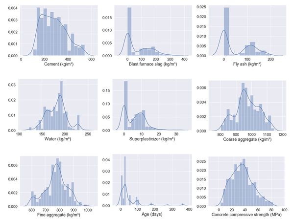
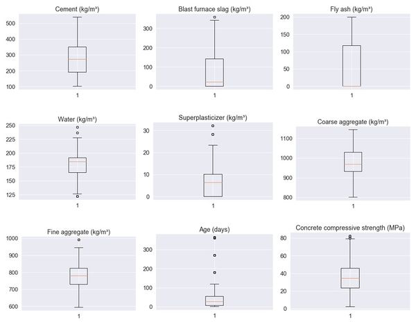
Histograms can help to form a better understanding of the data by showing information about each entry. The purpose of using histograms is to estimate whether the database has a normal distribution or whether it is biased to the left or right. The figures obtained assist the user to visualize and analyze the resources more effectively and facilitate the choice of the most suitable computational models [23]. Moreover, the density plots are variables that provide an idea of each feature distribution in the dataset. With these plots, one can see a smooth distribution curve drawn over the top of each histogram. Box plots are still another effective way to summarize the distribution of each available resource in the dataset. These boxes are useful because they give a better indication of the median value and the first and last quartile of the used data.

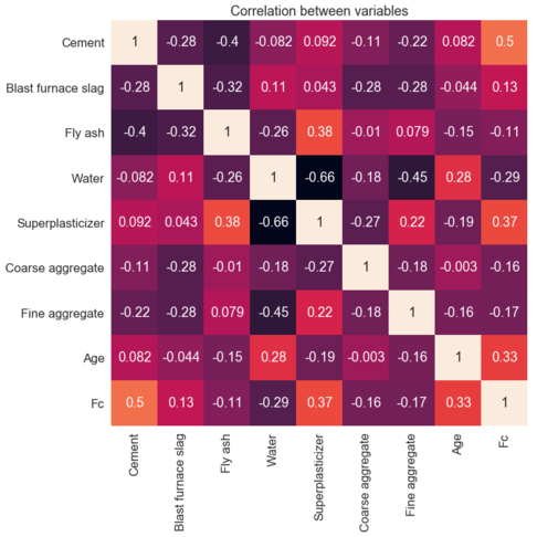
Finally, the correlation matrix is a factor that indicates how two variables are related in the dataset. This matrix describes the relationship between any pair of variables. In this matrix, it is possible to see whether the variables are positively or negatively correlated. The value obtained represents how closely these data are related. The correlation matrix can provide better insight into how the regression model can be used. Highly correlated input variables can affect the performance of specific algorithms [24].

The dataset needs to be pre-processed before its application. Pre-processing techniques have been proven effective and can improve the performance of computational models [25]. In this project, the database was pre-processed using the feature scale method. This method involves transforming all characteristics on a standard scale [26,27]. Usually, resources are transformed within a range between 0 and 1. The scale is necessary to construct the machine learning model because the Euclidean distance between points may lead to a domination point, having a more significant effect on the variable target.

To obtain better results, the database is usually split into training and testing data. Thus, the algorithm is trained with a volume of data that is validated in the test set. This is done to guarantee that the result obtained is not biased and only learns from similar data used for training. The dataset is reorganized with re-sampling. In this work, cross-validation and GridsearchCV are used. There are several types of cross-validation. However, the most common is the k-fold method. In this method, several samples k are created, each sample being set aside while the model trains with the remainder. The process repeats until it is possible to determine the “quality” of each observation. The most common values for the number of samples are between 5 and 10. This technique is most commonly used when the amount of data is lower or not sufficient to obtain a good result with more straightforward divisions [24–26].

The GridsearchCV is used as a tuning process that uses hyper-parametrization to determine the optimal values for a given model. This means that the performance of the entire model is based on the values of a specified hyper-parameter. GridsearchCV performs an exhaustive search on the specified parameters. This method is computationally expensive but produces excellent results [28,29].

2.2. Methods

2.2.1. Random forest

Random Forest models are constructed from a collection of decision trees [30,31]. They are easy to use without many pre-processing strategies. The idea is to build a collection of trees with a controlled variation. Random Forest is a clustering technique that can perform regression and classification tasks using multiple decision trees and bootstrap aggregation, commonly known as bagging. Bagging, in the Random Forest method, involves training each decision tree with a different data sample, where sampling is done with a substitution.The biggest problem with decision trees is that they tend to over-fit training data. Error pruning is the most common technique for avoiding this type of problem [32]. In this project, the Random Forest model is defined with the help of GridsearchCV.

2.2.2. Support vector machine

SVM are popular learning algorithms that work in classification and regression problems. In addition to performing linear regression and classification, SVM have also worked well on nonlinear data [33,34]. To sort linearly separable data, there may be different hyperplanes that can separate the data. The problem here would be to find a hyper-plane (margin) that could maximize the separation between two classes [35]. Therefore, SVM can be defined as a machine learning technique that can be used for regression and classification problems. This technique builds a multidimensional hyper-plane space to separate a dataset into different classes.

This paper used a support vector regressor as a non-parametric regression technique that relies solely on kernel functions. The goal is to find a function $f(x)$ that deviates from $y_{n}$ by a value no larger than $\varepsilon$ for each of the training points in our dataset and remains as flat as possible [34–36].

As the dataset is a multivariate supervised dataset, some of the cores used for regression comparison could be linear, polynomial, or RBFs [37]. In this project, GridsearchCV is used to evaluate possible kernels, linear, polynomial and RBFs. Thus, it is possible to assess the performance of these cores and evaluate different parameters of $\varepsilon$, which are the penalty parameters for the error. For polynomial and RBF kernels, there is a $\gamma$ parameter called the kernel coefficient. The best performance is evaluated based on the results of $R^{2}$. Thus, it is possible to assess the best performance of the implemented model using different kernels, $\varepsilon$ values and $\gamma$ parameters.

2.2.3. Artificial neural network

ANN are a typical example of a modern method that solves various engineering problems that could not be explained by traditional methods. The neural network can collect, memorize, analyze and process a large amount of data obtained through experimental tests [38,39]. Training data are critical to the network as they convey the information needed to find the optimal operating point. ANN are one of the most useful computational models used in supervised regression tasks and learning classification and works primarily with three layers: the input layer, the hidden layers and the output layer. However, the performance of an ANN depends mostly on the performance of hidden layers.

The number of neurons in the input layer is a pattern usually presented to the neural network. Each neuron in the input layer must represent an independent variable that affects the outcome of the network. Therefore, the number of nodes in the input layer is equal to the number of inputs.

Problems that require two or more intermediate layers are unusual. A neural network with two intermediate layers can represent functions of any shape. Therefore, there are no theoretical reasons for using more than two middle layers. However, the higher the number of layers of neurons, the better the performance of the neural network. This is because it increases learning capacity [40]. Also, the input layer may have a particular neuron called bias that increases the degrees of freedom, allowing the neural network to better adapt to the knowledge.

The number of neurons in the output layer is directly related to the task that the neural network performs. In general, the number of neurons the classifier must have is equal to the number of distinct groups.

When ANN are built, it is important to consider a suitable model architecture. In an ANN, neurons appear as

$z=w^{T}X+b$

(1)

followed by the activation function that determines whether the neuron is dispensed or follows to the output presented in the following equation

${\overset {\mbox{ˆ}}{y}}=a(z)=a(w^{T}X+b)$

(2)

However, it needs to train the neural network and evaluate the results using some function error and propagate through the neural network by updating weights ($w$) and bias ($b$). Therefore, derivatives of activation functions are used.

2.3. Performance parameters

To better evaluate the performance of predicting models, two different indicators are introduced, which are respectively defined as

* Root Mean Squared Error (RMSE)

$RMSE={\sqrt {MSE}}={\sqrt {{\frac {1}{N}}\sum _{i=1}^{N}{({y}_{i}-{\hat {y}})}^{2}}}$

(3)

* Coefficient of determination R-Squares (${R}^{2})$

${R}^{2}=1-{\frac {\sum _{i=1}^{N}{({y}_{i}-{\hat {y}})}^{2}}{\sum _{i=1}^{N}{({y}_{i}-{\overline {y}})}^{2}}}$

(4)

where ${\textstyle {\hat {y}}}$ is the predicted value of ${\textstyle y}$ and ${\textstyle y}$ is the average value of ${\textstyle y}$, ${\textstyle {\overline {y}}}$ is the mean value of all the measured values and ${\textstyle N}$ is the total number of the samples in the data set.

3. Simulation results and analysis

3.1. Database

As already said, this work required the acquisition of experimental data to determine the compressive strength of concrete through computational intelligence. The database chosen was obtained from studies by Yeh [22]. This database presents 1030 experimental stress versus compression tests. Eight input variables were used as shown in follows:

* cement;

* blast furnace slag;

* fly ash;

* water;

* superplasticizer;

* coarse aggregate;

* fine aggregate;

* age.

The output variable is the compressive strength of concrete ($F_{c}$).

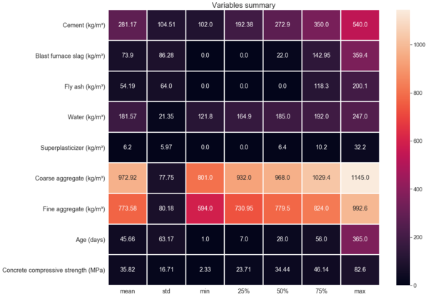
Figure 1 shows the static parameters, such as maximums and minimums of input and output components. The figure presents a heatmap, which graphically represents the measured value of numerical data using a color scheme, with warm colors representing the high-value of data points and cold colors representing the low-value data points of the data set.

Figure 1. Statistics parameters of data

It can be seen that the presented database, provided by Yeh [22], is quite consolidated and has a proper distribution for input and output variables. This fact facilitates the application of computational methods such as those presented in this work. There are also several studies in the literature that use the same database, so that a fair comparison between their results and the results obtained here can be made.

A visualization of histograms, density boxes and box plots obtained from the database used is provided in Figure 2. As stated earlier, this visualization aims to give a better idea of which method is more appropriate to obtain a better fit for the machine learning models. The variables have an almost normal distribution. Thus, it is possible to see that the efficiency of learning algorithms can be facilitated.

Figure 2. Histograms and density plots

Figure 3 shows the box plots for the variables used. An analysis of the outlier values for each input and output variable was also performed and the results are listed in Table 1. A proper distribution can be seen with no more than 10% of outliers in any attribute.

Figure 3. Box plot

Table 1. Analysis of outliers

Model attributes	Values
	Number of outliers	Percentage of outliers
Cement (kg/m³)	0	0.00
Blast furnace slag (kg/m³)	2	0.19
Fly ash (kg/m³)	0	0.00
Water (kg/m³)	9	0.87
Superplasticizer (kg/m³)	10	0.97
Coarse aggregate (kg/m³)	0	0.00
Fine aggregate(kg/m³)	5	0.49
Age (days)	59	5.73
Compressive strength of concrete (MPa)	4	0.39

Figure 4 presents the correlation matrix of the data used in the model. The correlation matrix shows no correlation between the variables used in the computational model. Therefore, it can be said that the components are mostly independent of each other.

Figure 4. Correlation matrix

To build up the used predictive models, the collected experimental data was split into two parts, the training set and the testing set. The training set is used to produce the final strong learner and the testing set is used to show the accuracy of the model in predicting the compressive strength. The results presented in this paper used 85% of the data (875 samples) for training the computer models; the remaining 15% of the data (155 samples) were used for testing. It is worth emphasizing that cross-validation was used to select the best parameters for each method, so there was not necessary to use the data validation set.

3.2. Random Forest

For the Random Forest machine learning model, the best parameters to be used in the kernel were defined after several tests. GridsearchCV and cross-validation were used to find a better correlation with the database and the model and to prevent overfitting of the models. Table 2 present the range of parameters used in the GridsearchCV and the best parameters used in the experiments for the Random Forest algorithm.

Table 2. Range of parameters and best parameters used in the Random Forest experiments

Parameter	Range	Setting
Maximum depth	4-10	10
Maximum of leaf nodes	100-120	120
Minimum number of samples required to split	7-9	7
Number of trees in the forest	400-500	500

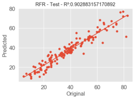
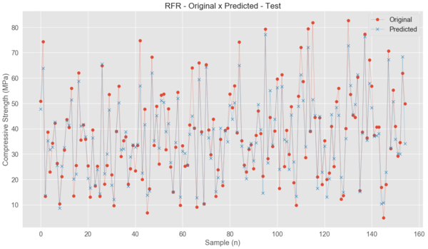
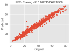
Figure 5 shows the graphical representation of the results of the test dataset. The original values are those obtained experimentally and the predicted values are the values obtained by the Random Forest model. Figure 6 presents the relationship between the predicted compressive strength values and the tested compressive strength values for the training and testing sets. For both sets, the graphs display a linear relationship between the predicted and testes values, especially for the training set. The figure also displays the value of $R^{2}$.

Figure 5. Original versus expected results for the Random Forest

Figure 6. Relationship between tested and predicted compressive strength for the Random Forest

The Random Forest model shows excellent performance in predicting compressive concrete strength values. For the training data set, performance indicators are $R^{2}=0.964$ and $RMSE=3.087$ MPa, which means that the predicted value and original values of the experiment are almost the same. The test data set shows $R^{2}=0.902$ and $RMSE=5.614$ MPa. The error ratio is very low and indicates that the Random Forest model is well suited for engineering practice.

3.3. Support vector machine

For the SVM learning model, the best parameters to be used in the kernel were defined. As GridsearchCV was used in this work to evaluate possible kernels, linear, polynomial and RBFs could be applied. The intention was to evaluate the performance of these cores in the database presented and estimate different parameters of $\varepsilon$, which are the penalty parameters for the error. For polynomial and RBF kernels, there is also a kernel coefficient called the $\gamma$ parameter. In such cases, there is a need to search these parameters to find the relationships between them and the best metrics that can optimally predict relevant results for the database.

By applying linear, polynomial and RBFs, it was found that the RBF was the best SVM kernel, i.e., which best predicts the results for the data presented. The best performance is evaluated based on the results of $R^{2}$. Thus, it is possible to evaluate the best performance of the model over different kernels, $\varepsilon$ values and $\gamma$ parameters. Table 3 presents the range of parameter used in the GridsearchCV and the best parameters used in the experiments for the SVM algorithm.

Table 3. Range of parameters used and best parameters for the SVM experiments

Parameter	Range	Setting
C	10-500	100
Degree	3-5	3
Epsilon	0.1-1	0.1
Kernel	RBF-Linear-Sigmoid	RBF

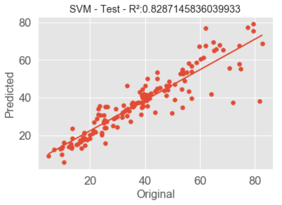
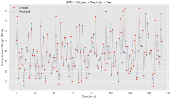
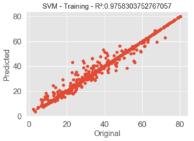
Figure 7 shows the graphical representation of the results of the test dataset. Figure 8 presents the relationship between the predicted compressive strength values and the tested compressive strength values for the training and testing sets. The relationship between the predicted and testes values can be considered linear for both sets, especially for the training set results. The figure also shows the values of $R^{2}$.

Figure 7. Original versus expected results for the SVM

Figure 8. Relationship between tested and predicted compressive strength for the SVM

The SVM model shows good performance in calculating compressive concrete strength values. For the training data set, $R^{2}=0.976$ and $RMSE=2.554$ MPa mean that the predicted value and original values of the test are very close. The test data set shows $R^{2}=0.829$ and $RMSE=7.456$. The error ratio is low and, despite being larger than that found by the Random Forest, it also indicates that the SVM model is suitable for engineering practice. However, this method does not seem to be the best suited for this database.

3.4. ANN

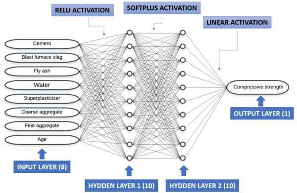
The current model used Keras, an open-source neural network library available in Python. Keras was used on the TensorFlow backend [41,42]. The neural network was trained using the SGD optimizer. The defined architecture with the best result is presented, as can be seen in Figure 9.

Figure 9. Schematic representation of the ANN

Eight neurons were used for the input layer. Further, 2 intermediate layers with 10 neurons each were used. One neuron was used in the output layer (the compressive strength of the concrete). The activation functions for the initial and intermediate layers are ReLU. This decision was made based on its well-known performance for regression problems [43,44]. It was necessary to use a linear activation function in the last layer because the method is regression [45]. Glorot uniform was used to initialize the weights, with small numbers close to 0 [46].

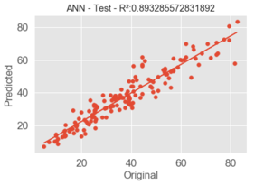
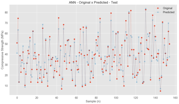
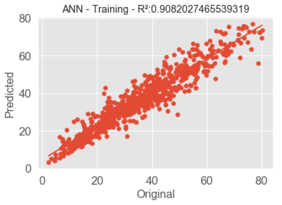
Figure 10 shows the graphical representation of the results of the test dataset, where the original and predicted values are compared. Figure 11 presents the relationship between the predicted compressive strength values and the tested compressive strength values for the training and testing sets. For both two sets, a linear relationship between the predicted and testes values is obtained. The figure also shows the values of $R^{2}$ for both sets.

Figure 10. Original versus expected results for the ANN

Figure 11. Relationship between tested and predicted compressive strength for the ANN

The ANN model shows a good performance in predicting compressive concrete strength values. For the training data set, $R^{2}=0.908$ and $RMSE=4.979$ MPa, which means the predicted value and original values of the test are comparable. The test data set shows $R^{2}=0.893$ and $RMSE=5.881$ MPa. The found error ratio is low and indicates that ANN is appropriate for engineering practice too. However, it is worth saying that the ANN model spent, among the tested models, the highest processing time with the applied database.

The summaries of the performance values obtained for the training set are summarized in Table 4. The table presents the $R^{2}$, the RMSE and the runtime for the three methods used.

Table 4. Comparison of obtained results

	$R^{2}$	RMSE (MPa)	Execution time (seconds)
Random forest	0.902	5.614	5.506
SVM	0.829	7.456	0.247
ANN	0.893	5.881	86.46

The best model, measured by the chosen performance parameters, was the Random Forest. This may be due to the fact that the random forest algorithms are known to be simpler to use and have a high learning rate. ANN algorithms still show good results and was second for the performance techniques chosen in this work. However, as seen, they have significantly higher CPU time.

The results for the testing set parameters results are also compared to some previous studies using Random Forest, SVM and ANN algorithms with the same Yeh’s dataset, as shown in Table 5.

Table 5. Comparison with the results for the same dataset in previous studies

Research	Algorithm	$R^{2}$	RMSE (MPa)
Chou et al. [19]	ANN	0.88	-
	SVM	0.91	-
Chou et al. [20]	ANN	-	7.9
	SVM	-	5.5
Young et al. [21]	Random Forest	0.86	5.7
	ANN	0.82	6.3
	SVM	0.83	6.4
This paper	Random Forest	0.90	5.6
	SVM	0.83	7.5
	ANN	0.89	5.9

The RMSE performance results obtained in this study are slight better than the results obtained in previously studies. The overall performance results obtained are significantly better for ANN and Random Forest. However, the same behavior does not happen for SVM. Nonetheless, the performance results obtained for this type of algorithm is still consistent with those obtained in the existing literature.

4. Conclusions

This work aimed to present the study of computational intelligence applied to define the concrete compressive strength from a database obtained in the studies of Yeh [22]. Three computational methods of machine learning and artificial intelligence were used, namely Random Forest, Support Vector Machines and Artificial Neural Networks. Data pre-processing and data visualization methods were also used to improve the results. Preprocessed methods known as GridsearchCV and cross-validation were employed to improve the performance of machine learning methods.

The obtained results show that the Random Forest gave the best performance ($R^{2}=0.902$ and $RMSE=5.614$) and an average execution time. It can be noted that the SVM method had the worst performance of the three used methods but presented the shortest execution time. On the other hand, the ANN showed the second-best result and the longest execution time. The overall error rate can be considered low and the techniques can adequately be used to predict the concrete compressive strength, staying within the acceptable safety range for engineering practices.

The computational intelligence models used are reliable to solve different complex problems, such as prediction problems. These models can be used to solve a specific problem when a deviation in available data is expected and accepted, and when a defined methodology is not available. Therefore, to predict the properties of concrete with high reliability, instead of using expensive experimental investigation, conventional and innovative models can be replaced by computational intelligence models.

Computational intelligence models can be used to predict the compressive strength of concrete specimens, as shown in this study. The prediction of mean percent error values for these simulations shows a high degree of consistency with compressive strength and is experimentally evaluated from the concrete specimens used. Thus, the present study suggests an alternative approach to evaluate compressive strength against destructive testing methods.

Acknowledgments

CAPES and CEFET-MG supported the work described in this paper.

References

[1] Hibbeler R.C.C. Resistência dos materiais. 7th ed., Pearson, São Paulo, SP, 2010.

[2] Babanajad S.K. Application of genetic programming for uniaxial and multiaxial modeling of concrete. Springer, Switzerland, 2015.

[3] Hoang N.D., Tran X.L., Le C.H., Nguyen D.T. A backpropagation artificial neural network software program for data classification in civil engineering developed in .NET Framework, DTU J. Sci. Technol. 03, 51–56, 2019.

[4] Reuter U., Sultan A., Reischl D.S. A comparative study of machine learning approaches for modeling concrete failure surfaces. Adv. Eng. Softw., 116:67–79, 2018.

[5] Torky A.A., Aburawwash A.A. A deep learning approach to automated structural engineering of prestressed members. Int. J. Struct. Civ. Eng., 7:347–352, 2018.

[6] Sun Z., Li K., Li Z. Prediction of concrete compressive strength based on principal component analysis and radial basis function neural network prediction of concrete compressive strength based on principal component analysis and radial basis function neural network. IOP Conf. Ser. Mater. Sci. Eng., 2019.

[7] Asteris P.G., Mokos V.G. Concrete compressive strength using artificial neural networks. Neural Comput. Appl., 32:11807–11826, 2020.

[8] Rajeshwari R., Mandal S. Prediction of compressive strength of high-volume fly ash concrete using artificial neural network. Lect. Notes Civ. Eng., 25:471–483, 2019.

[9] Feng D.C., Liu Z.T., Wang X.D., Chen Y., Chang J.Q., Wei D.F., Jiang Z.M. Machine learning-based compressive strength prediction for concrete: An adaptive boosting approach. Constr. Build. Mater., 230:117000, 2020.

[10] Armaghani D.J., Asteris P.G. A comparative study of ANN and ANFIS models for the prediction of cement-based mortar materials compressive strength. Springer London, 2020.

[11] Duan Z.H., Kou S.C., Poon C.S. Prediction of compressive strength of recycled aggregate concrete using artificial neural networks. Constr. Build. Mater., 40:1200-1206, 2013.

[12] Siddique R., Aggarwal P., Aggarwal Y. Prediction of compressive strength of self-compacting concrete containing bottom ash using artificial neural networks. Adv. Eng. Softw., 42:780–786, 2011.

[13] Naderpour H., Rafiean A.H., Fakharian P. Compressive strength prediction of environmentally friendly concrete using artificial neural networks. J. Build. Eng., 16:213–219, 2018.

[14] Chithra S., Kumar S.R.R.S., Chinnaraju K., Alfin Ashmita F. A comparative study on the compressive strength prediction models for High Performance Concrete containing nano silica and copper slag using regression analysis and Artificial Neural Networks. Constr. Build. Mater., 114:528-535, 2016.

[15] Chou J.-S.S., Tsai C.-F.F. Concrete compressive strength analysis using a combined classification and regression technique. Autom. Constr., 24:52–60, 2012.

[16] Pham, A.D., Hoang N.D., Nguyen Q.T. Predicting compressive strength of high-performance concrete using metaheuristic-optimized least squares support vector regression. J. Comput. Civ. Eng., 30:28–31, 2016.

[17] Omran B.A., Chen Q., Asce A.M., Jin R. Comparison of data mining techniques for predicting compressive strength of environmentally friendly concrete. J. Comput. Civ. Eng., 30(6), 2016.

[18] Nguyen K.T., Nguyen Q.D., Le T.A., Shin J., Lee K. Analyzing the compressive strength of green fly ash based geopolymer concrete using experiment and machine learning approaches. Constr. Build. Mater. 247:118581, 2020.

[19] Chou J., Chiu C., Farfoura M., Al-taharwa I. Optimizing the prediction accuracy of concrete compressive strength based on a comparison of data-mining techniques. J. Comput. Civ. Eng., 25(3). 2011.

[20] Chou J.S., Tsai C.F., Pham A.D., Lu Y.H. Machine learning in concrete strength simulations: Multi-nation data analytics. Constr. Build. Mater., 73:771–780, 2014.

[21] Young B.A., Hall A., Pilon L., Gupta P., Sant G. Can the compressive strength of concrete be estimated from knowledge of the mixture proportions?: New insights from statistical analysis and machine learning methods. Cem. Concr. Res., 115:379–388, 2019.

[22] Yeh I.-C. Modeling concrete strength with augment-neuron networks. J. Mater. Civ. Eng., 10(4), 1998.

[23] Scott D.W. On optimal and data-based histograms. Biometrika, 66:605–610, 1979.

[24] Steiger J.H. Tests for comparing elements of a correlation matrix. Psychol. Bull., 87:245, 1980.

[25] Wang L., Wang G., Alexander C.A. Big data and visualization: methods, challenges and technology progress. Digit. Technol., 1:33–38, 2015.

[26] Forman G. BNS feature scaling: an improved representation over tf-idf for svm text classification. In: Proc. 17th ACM Conf. Inf. Knowl. Manag., ACM, pp. 263–270, 2008.

[27] Zhang M.-L., Zhou Z.-H. Improve multi-instance neural networks through feature selection. Neural Process. Lett., 19:1–10, 2004.

[28] Buitinck L., Louppe G., Blondel M., Pedregosa F., Mueller A., Grisel O., Niculae V., Prettenhofer P., Gramfort A., Grobler J., Layton R., Vanderplas J., Joly A., Holt B., Varoquaux G. API design for machine learning software: experiences from the scikit-learn project. ArXiv Prepr. ArXiv1309.0238, 1–15, 2013.

[29] Pedregosa F., Varoquaux G., Gramfort A., Michel V., Thirion B., Grisel O., Blondel M., Prettenhofer P., Weiss R., Dubourg V. Scikit-learn: machine learning in python. J. Mach. Learn. Res., 12:2825–2830, 2011.

[30] Barandiaran I., Ho T.K. The random subspace method for constructing decision forest. IEEE Trans. Pattern Anal. Mach. Intell., 20:832–844, 1998.

[31] Pal M. Random forest classifier for remote sensing classification. Int. J. Remote Sens., 26:217–222, 2005.

[32] Breiman L. Random forests. Mach. Learn., 45:5–32, 2001.

[33] Lin C.-F., Wang S.-D. Fuzzy support vector machines. IEEE Trans. Neural Networks., 13:464–471, 2002.

[34] Scholkopf B., Smola A.J. Learning with kernels: support vector machines, regularization, optimization, and beyond. IEEE Trans. Neural Networks, 16:781–781, 2001.

[35] Suykens J.A.K., Vandewalle J. Least squares support vector machine classifiers. Neural Process. Lett., 9:293–300, 1999.

[36] Drucker H., Burges C.J.C., Kaufman L., Smola A.J., Vapnik V. Support vector regression machines. In: Adv. Neural Inf. Process. Syst., pp. 155–161, 1997.

[37] Basak D., Pal S., Patranabis D.C. Support vector regression. Neural Inf. Process. Rev., 11:203–224, 2007.

[38] Hopfield J.J. Artificial neural networks. IEEE Circuits Devices Mag., 4:3–10, 1988.

[39] Sarle W.S. Neural networks and statistical models. Proc. Ninet. Annu. SAS Users Gr. Int. Conf., 1994.

[40] Arruda V.F., Moita G.F., Silva P.F.S. Determining the optimal artificial neural network architecture capable of predict the compressive strength of concrete. Proc. XL Ibero-Latin-American Congr. Comput. Methods Eng., 2019.

[41] Goldsborough P. A tour of tensorflow. ArXiv Prepr. ArXiv1610.01178, 2016.

[42] Kossaifi J., Panagakis Y., Anandkumar A., Pantic M. Tensorly: Tensor learning in python. J. Mach. Learn. Res., 20:925–930, 2019.

[43] Clevert D.A., Unterthiner T., Hochreiter S. Fast and accurate deep network learning by exponential linear units (ELUs). 4th Int. Conf. Learn. Represent. ICLR 2016 - Conf. Track Proc., 1–14, 2016.

[44] Klambauer G., Unterthiner T., Mayr A., Hochreiter S. Self-normalizing neural networks. Adv. Neural Inf. Process. Syst., 972–981, 2017.

[45] Agarap A.F. Deep learning using rectified linear units (relu). ArXiv Prepr. ArXiv1803.08375, 2018.

[46] Kaveh A., Kalateh-Ahani M., Fahimi-Farzam M. Constructability optimal design of reinforced concrete retaining walls using a multi-objective genetic algorithm. Struct. Eng. Mech., 47:227–245, 2013.