A mis padres
Abstract
Most of the existing materials around us can be considered composite materials, since they are composed by several phases or components at certain spatial scale. The physical and chemical properties of composites, as occurs with structures composed by two or more materials, is defined by the response provided by their constituents. Therefore, a good characterization of the composite requires considering the performance of its components. In the last decades, several methods have been proposed with this approach to characterize composite materials, most of them based on multiscale techniques.
Nowadays, multiscale homogenization analysis is a popular topic in the simulation of composite materials. This is because the complexity of new composites demands of advanced analysis techniques for their correct characterization, and thanks to the continuous increase of computational capacity. However, the computational cost when multiscale procedures are taken to the non-linear range and are applied to real-size structures is still excessively high. In this context, this monograph presents a comprehensive homogenization formulation for an efficient non-linear multiscale modeling of composite structures.
The development of a composite multiscale constitutive model is addressed from two different homogenization approaches. The first one corresponds to a phenomenological homogenization procedure for the non-linear analysis of carbon nanotubes reinforced composites. The second one is a general two-scale homogenization procedure to analyze three-dimensional composite structures.
Carbon nanotubes (CNTs) have been regarded as ideal reinforcements for high-performance composites. The formulation developed takes into account explicitly the performance of the interface between the matrix and the CNTs. The load is transferred to the nanotubes through the considered interface. The composite non-linear behavior results from the non-linearities of its constituents, and in case of interface damage, it also becomes non-linear the law defined to couple the interface with the CNTs. The formulation is validated studying the elastic response and non-linear behavior of several composites.
In the context of multiscale homogenization, a first-order and an enhanced-first-order formulation is developed. The results obtained for laminate composites using the first-order formulation are compared with other microscopic formulations, showing that the homogenization method is an excellent alternative when microstructural effects must be taken into account. Then, a strategy to conduct non-linear multiscale analysis in an efficient way is proposed. The procedure conserves the dissipated energy through the scales and is mesh independence. The analysis of academic examples is used to show the capacity of the non-linear strategy. Finally, the simulation of an industrial composite component proves the performance and benefits of the non-linear homogenization procedure developed.
Acknowledgements
This work was financially supported by CIMNE together with the European Community under grant:
NMP-2009-2.5-1 246067 M_RECT “Multiscale Reinforcement of Semi-crystalline Thermoplastic Sheets and Honeycombs”,
FP7-PEOPLE-2013-IRSES 612607 TCAiNMaND “Tri Continental Alliance in Numerical Methods applied to Natural Disasters”, by European Research Council through of Advanced Grant:
ERC-2012-AdG 320815 COMP-DES-MAT “Advanced tools for computational design of engineering materials”, by Dirección General de Investigación Científica y Técnica:
MAT2014-60647-R OMMC “Optimización multi-escala y multi-objetivo de estructuras de laminados compuestos”, by ``Abengoa Research”, and by Universitat Politecnica de Catalunya (UPC).
All this support is gratefully acknowledged.
List of Acronyms
| BVP | Boundary Value Problem |
| CNTs | Carbon Nanotubes |
| CVD | Chemical Vapor Deposition |
| DDM | Discrete Damage Mechanics |
| EFO | Enhanced-First-Order |
| FE | Finite Element |
| FEM | Finite Element Method |
| FE2 | Finite Element Two-Scale |
| FO | First-Order |
| IFSS | Interfacial Shear Strength |
| LE | Linear Element |
| MWCNTs | Multiwall Carbon Nanotubes |
| NLAF | Non-Linear Activation Function |
| NLS | Non-Linear Strategy |
| OpenMP | Open Multi-Processing |
| POD | Proper Orthogonal Decomposition |
| QE | Quadratic Element |
| RHS | Right-Hand Side |
| RVE | Representative Volume Element |
| SFS | Smart First Step |
| SP | Serial-Parallel |
| SWCNTs | Single Wall Carbon Nanotubes |
Introduction
The continuum mechanics theory has made a great effort to obtain the behavior of homogeneous materials using physical and mathematical concepts showing a good agreement with reality. Furthermore, the constant improvements on computer technology and computer architecture have allowed to improve the numerical tools used to simulate mechanical structures. In the numerical simulation field, one of the most extended methods used for several applications is the Finite Element Method (FEM) [1]. In a FEM analysis the behavior of the homogeneous materials in the structure is simulated by a specific constitutive law or constitutive model with some calibrated parameters.
Composites are non-homogeneous materials formed by two or more different components which can be homogeneous materials or even micro-heterogeneous materials. The homogenized behavior of the composites depends strongly on the internal spatial distribution, the size and the properties of the material components and their respective interfaces. Therefore, composites require more complex and advanced constitutive models than the ones use in single materials.
For a linear analysis or a structural analysis to failure study it is enough to simulate the composite with one orthotropic homogenized characterization and a constitutive law with some complexity. However, more realistic composite constitutive models are necessary to simulate the structures beyond their elastic limit, to obtain the post critic behavior of these or to estimate their tenacity and structural integrity.
The direct application of the FEM is not the most appropriate or effective manner to face the described problem. In a classical FEM analysis each component material has its own constitutive model. Therefore, the numerical model of the structure must to be discretized with a Finite Element (FE) size of at least the size of the components in the composite. In general, this restriction gives as result FE meshes with large number of finite elements which demand an extremely expensive computational cost, and in some cases this analysis is unfeasible to perform. Consequently, to analyze composite structures and to characterize their behavior or fracture modes more suitable strategies must be developed.
Background and motivation
The complexity of the composite materials has promoted that several formulations appeared to predict their behavior, which are more o less suitable according to the computational cost required, the accuracy in the results desired or even the expected failure type. Further, the development of a new generation of composites with improved properties, more reliable and cheap has extended its use to many industrial applications.
The phenomenological homogenization methods are a possibility to analyze composite materials with a heterogeneous internal structure. In this context, the most usual method is the classical mixing theory proposed initially by Truesdell and Toupin [2]. The formulation obtains the homogenized behavior of the composite through the compatibility equation and from the mechanical performance of the component materials, which are simulated with their own constitutive laws. Later, several modifications and extensions of this classical theory of mixtures have enabled the resolution of any composite with reinforced matrix, without the limitation required by the compatibility equation [3].
One of the most significant modifications of the mixing theory is the Serial-Parallel (SP) continuum approach. In the SP formulation the mechanic characteristic of the composite is obtained using not only the properties and constitutive model of the material components but also taking into account their topological distribution [4]. The SP mixing theory assumes a serial-parallel self-adjusting behavior to the topological distribution of fiber embedded in the matrix of the composite material. This approach imposes the iso-strain condition in the fiber alignment direction on the components of the composite (as parallel materials) and the iso-stress condition in the orthogonal direction (as serial materials).
The reinforcements developed today, as the nanofibers or Carbon Nanotubes (CNTs) and the renewed composites as the reinforced concrete with short fibers, require sophisticated formulations for their simulation. The interface zone between matrix and reinforcement has a meaningful effect in the final properties and response of the composite structures made with these current composites. Many effort have been made to consider the debonding phenomenon in laminated composites but it is not enough to totally characterize the behavior of these micro-heterogeneous composites. Therefore, renovated formulations or renewed modifications of existing theories should be developed to face with the challenge of predict the behavior of these new composites.
The homogenization techniques are another option to analyze composite materials. In these methods the characterization of the entire composite is obtained through the analysis of its internal structure or microscopic structure. In this context, an approach extensively used is the called multiscale homogenization method. In general, the formulation is based on the use of the concept of unit cell or Representative Volume Element (RVE) [5]. The definition of the RVE corresponds with a microscopic subregion which is representative of the entire micro-structure (referred as micro-scale) level of the composite. This is employed to determine the homogenized properties and behavior of the composite level (also known as macro-scale). It is assumed that the RVE must contain a sufficient number of inclusions to make the homogenized moduli independent of homogeneous forces or displacements on the RVE boundary.
Within this context, one of the most extended and popular method is the known first-order homogenization approach [6]. This multiscale method uses the macro-scale deformation gradient tensor (or the strain tensor) to solve the micro-scale problem. The composite behavior (the macro-scale stress-strain relationship) is obtained by a detailed modeling of the internal heterogeneous structure of the composite in the RVE. Therefore, the approach does not require any composite constitutive assumption or compatibility equation to address the composite response. Moreover, there are not restriction about the constitutive law of the component materials, even non-linear materials and time-dependency models can be taken into account. The benefits of the method becomes in a challenge when a non-linear analysis of a three-dimensional structure is studied. Considering a homogenization technique [7], it is required for each time step to solve one RVE at each point of integration at the macro-scale because the non-linear threshold and non-linear behavior of the homogenized composite are unknown. Therefore, the computational cost in the non-linear analysis of an industrial component by using multiscale homogenization is extremely expensive, and in many cases, is unsuitable to perform.
In addition to the computational cost to address the non-linear problem with multiscale homogenization methods, the softening issue must be considered too. The non-linear constitutive law of the component materials are defined in the RVE problem. Consequently, the non-linear behavior starts in the micro-scale and then, it moves up to the macro-scale. Because of this, novel computationally efficient multiscale strategies dealing with non-linear problem should be developed taking into account also the conservation of the dissipated energy through the scales. Besides, they must be macro and micro mesh independence for the case of homogenization.
In the last decade, a second-order computational homogenization was proposed as a natural extension of the first-order homogenization method [8]. It was developed to be applied in critical regions of intense deformation, where the characteristic wave length of the macro-scale deformation field is of the order of the size of the micro-scale. Therefore, in this approach the macroscopic gradient of the deformation gradient is also incorporated in the microscopic scale problem. The first-order equilibrium problem is conserved in the micro-scale though a higher-order equilibrium problem appears in the macro-scale. The solution of the proposed multiscale approach is made through a complex finite element implementation, which restricted its popular application.
The main advantage of the described second-order homogenization is that it can consider intense localization phenomena, then it is a desirable approach for non-linear analysis. On the other hand, the benefit of the first-order homogenization is that it considers first-order equilibrium equations at both scales, which represents an advantage from a point of view of computational implementation. Therefore, an enhanced-first-order approach could be an interesting option to account second-order effects of the macro-scale from the micro-scale by the incorporation of macroscopic second-order deformation measure in the microscopic boundary value problem.
Objectives
The main objective of this study is to develop a comprehensive formulation for the analysis of three-dimensional composite structures in linear and non-linear range. In this context, the partial targets to address the global aim of this monograph can be written in a synthesized form as:
- Development of a phenomenological homogenization formulation based on the mixing theory for the analysis of CNTs reinforced composites. The formulation should consider the effect of the CNTs-matrix interface in the composite behavior.
- Extension to three dimensions of the first-order multiscale homogenization for the numerical analysis of composite structures. Implementation of an elimination of redundant unknowns method to solve the microscopic boundary value problem considering the constraint conditions on the boundary domain.
- Improvement of the first-order multiscale approach implemented to consider second-order effects in the microscopic scale from the macroscopic scale.
- Comparison of numerical simulations with other microscopic formulations to show the advantages and drawbacks of the developed first-order multiscale procedure.
- Development of a non-linear strategy to optimize the computational cost of the analysis of real-size composites structures using a multiscale homogenization approach.
In order to achieve the objectives described previously, there are parallel tasks that must be addressed. These are important milestones of this work that are worth to be mentioned. Among them:
- Parallel numerical implementation of the developed approaches through an Open Multi-Processing (OpenMP) philosophy in the finite element code PLCd [9].
- Development of a preprocessor manager to deal with the numerical models of the microstructure (RVE) using a GID problem type [10,11].
- Numerical validation of the different formulations implemented in PLCd through the simulation of several composites and by the analysis of real-structural components.
Outline
In the present monograph is possible to observe that from a theoretical point of view the main goal can be divided in two parts. For this reason, the document is arranged in two major self-contained parts.
In Part I a phenomenological homogenization model for the analysis of composites material using CNTs as reinforcement is presented. The formulation developed is based on the mixing theory. In this context, Chapter 2 shows a review of the state of the art of the classical mixing theory and its subsequent modifications while Chapter 3 introduces general considerations about the CNTs and a state of the art of the production methods and of the measured mechanical properties. Then, Chapter 4 presents the formulation and numerical implementation of the “ad hoc” homogenization model developed in this study. Chapter 5 shows the validation and numerical examples analyzed using the formulation proposed in the above chapter. Finally, in Chapter 6 the conclusions and future work about the model developed in this part of the monograph is approached.
In Part 6 the developed multiscale homogenization approach for composite structures is described. The state of the art is addressed in Chapter 8, which shows the fundamental theories and the latest developments about this research topic. Chapter 9 presents the formulations and implementations of the first-order homogenization and the proposed enhanced-first-order extension to consider second-order effects. In Chapter 10 the implemented two-scale homogenization procedure is compared with other micro-structural formulations. Chapter 11 describes the non-linear strategy proposed for multiscale approaches, also its validation and numerical applications are shown. The conclusions and future work of this second part are addressed in Chapter 12.
In the final conclusions chapter the achievements of the present study are exposed along with concluding remarks and future works derived from this monograph.
Research dissemination
The work included in this monograph resulted in the following scientific publications:
Part I
- F. Otero, S. Oller, X. Martinez and O. Salomon. Modelling of behaviour of carbon nanotube-reinforced composites. In: MATCOMP'11 - IX Congreso Nacional de Materiales Compuestos. Girona, España 2011.
- F. Otero, S. Oller, X. Martinez and O. Salomon. Numerical modelling of behaviour of carbon nanotube-reinforced composites. In: COMPLAS XI - XI International Conference on Computational Plasticity. Fundamentals and Applications. Barcelona, España, 2011.
- F. Otero, S. Oller, X. Martinez and O. Salomon. Modelling the elastic behavior of carbon nanotube-reinforced composites. In: Composites 2001 - 3rd ECCOMAS Thematic Conference on the Mechanical Response of Composites. Hannover, Germany, 2011.
- F. Otero, S. Oller, X. Martinez and O. Salomon. Modelling viscoelastic behaviour of carbon nanotube-reinforced thermo-plastics. In: MECOM 2012 - X Congreso Argentino de Mecanica Computacional. Salta, Argentina, 2012.
- F. Otero, X. Martinez, S. Oller and O. Salomon. Study and prediction of the mechanical performance of a nanotube-reinforced composite. Composite Structures. 2012, 94(9):2920-2930. doi: 10.1016/j.compstruct.2012.04.001.
Part II
- X. Martinez, F. Otero and S. Oller. Strategy for an efficient material non-linear multiscale analysis In: COMAT 2015 - VI International Conference on Science and Technology of Composite Materials. Buenos Aires, Argentina, 2015.
- F. Otero, S. Oller, X. Martinez and O. Salomon. Numerical homogenization for composite materials analysis. Comparison with other micro mechanical formulations. Composite Structures. 2015, 122:405-416. doi: 10.1016/j.compstruct.2014.11.041.
- F. Otero, X. Martinez, S. Oller and O. Salomon. An efficient multi-scale method for non-linear analysis of composite structures. Composite Structures. 2015, 131:707-719. doi: 10.1016/j.compstruct.2015.06.006.
- F. Otero, S. Oller and X. Martinez. Multiscale computational homogenization: review and proposal of a new enhanced-first-order method. Archives of Computational Methods in Engineering. 2016, 1-27. doi: 10.1007/s11831-016-9205-0
In addition, part of the work was presented at the following unpublished conferences:
- F. Otero, S. Oller, X. Martinez and O. Salomon. Numerical homogenization for the simulation of composites materials. Comparison with other micro mechanical formulations. Mechanics of Composites (MECHCOMP2014). Long Island, NY State, USA, 8-12 June 2014.
- F. Otero, S. Oller and X. Martinez. Non-linear multiscale strategy to analyze composite materials efficiently. 18th International Conference on Composites Structures (ICCS18). Lisbon, Portugal 15-18 June, 2015.
Finally, part of the work presented in this document is the result of the collaborating with external researchers during the following research stays:
- WVU-(West Virginia University), 6-month doctoral research stay. Worked under the direct supervision of Prof. Ever J. Barbero in the Mechanical and Aerospace Engineering of the Benjamin M. Statler College of Engineering and Mineral Resources, WVU. Morgantown, USA. January - June 2014. The following article resulted from the work developed during the stay: M.M. Moure, F. Otero, S.K. García-Castillo, S. Sánchez-Sáez, E. Barbero and E.J. Barbero. Damage evolution in open-hole laminated composite plates subjected to in-plane loads. Composites Structures. 2015, 133:1048-1057. doi: 10.1016/j.compstruct.2015.08.045.
- CIMAT-(Centro de Investigación en MATemáticas), 2-month research stay in the framework of the TCAiNMaND project, a Marie Curie International Research Staff Exchange Scheme (IRSES) under grant agreement FP7-612607. Worked under the direct supervision of Dr. Salvador Botello in the Computational Sciences Department of CIMAT. Guanajuato, México. November - Dicember 2015.
Part I. Phenomenological homogenization
1 Introduction
Composites are materials made of at least two different components. Generally, are constituted by a matrix that surrounds the reinforcing elements, which may be in the form of particles, nanotubes, short fibers, fibers, etc [12]. The main function of matrix component is to give cohesion, support the reinforcement and transfer the external actions to the reinforcements. While the main task of the reinforcement component is to improve the matrix properties. The appropriate design of structural elements made of this type of composite material requires the use of composite constitutive models capable of estimating their stiffness, strength and different failure modes.
In case of using fibers or nanotubes as reinforcement components, the performance of the composite depends on the achievement of the following four main characteristics:
- Aspect ratio of the fibers. The fiber aspect ratio is a dimensionless geometric measurement that results from dividing the length of the reinforcement by its diameter. This parameter is important because the stress distribution in the reinforcement depends on it [13]. In fibers with high aspect ratios the fiber end effect is less important. The reinforcement is considered to behave as a long fiber when its aspect ratio is larger than 1000.
- Dispersion of fibers in the composite. A uniform distribution of reinforcement in the composite is fundamental to ensure that it is completely surrounded by matrix. This is necessary to obtain an effective stress transfer. A good dispersion of the reinforcement in the composite also helps to have a more uniform stress distribution in it, reducing the regions susceptible having stress concentrations.
- Fiber alignment. It has been shown that the difference between random distribution and perfect alignment may represent a factor of five in the composite Young's modulus [14]. Fiber alignment also affects the isotropy of the composite, as perfect alignments increase its anisotropy.
- Load transmission from the matrix to the fiber. The last and probably most important factor is the interfacial tension between matrix and reinforcement. In general, the loads in a composite structure are introduced through the matrix and are transferred to the reinforcement through the interface [13]. Therefore, the interface can be defined as the region surrounding the reinforcement where this stress transfer takes place. The properties of the composite depend on the properties of this region, and on its ability to transfer the load efficiently.
On the other hand, the external load applied to a composite is shared disproportionately by the different components, as their elastic properties are different. In case of considering an iso-strain hypothesis [2] the stresses on the reinforcement will be larger than in the matrix, as the reinforcement is stiffer than the matrix. This unequal stress distribution generates shear stresses between both materials in a region that can is usually called the interface. The load transfer from the matrix to the reinforcement is produced in this region. Shear stresses in the interface increase proportionally to the external load until a critical value, beyond which the interface breaks. This critical value is known as Interfacial Shear Strength (IFSS) and it limits the stress transfer capacity.
In this context, the classical rule of mixtures was one of the first theories used to address a composite constitutive model from a phenomenological point of view [2]. The theory defines the manner in which all components interact to provide the material performance. The iso-strain hypothesis defined in the mixing theory implies a parallel distribution on the components in the composite. It is possible to think in an inverse mixing theory which replaces the iso-strain assumption by an iso-stress assumption, therefore it means a serial distribution on the components in the composite. The characterization of the composite depends of the hypothesis used in the formulation. Then, modifications of the mixing theory capable to consider all possible behaviors of the composite: parallel, serial and mixed were proposed [15]. Finally, the serial/parallel concept was introduced in the theory, which replaced the iso-strain hypothesis by an iso-strain condition in the fiber direction and iso-stress condition in the transversal directions [4].
The mixing theory began to be considered as a constitutive equation manager when its hypothesis were coupled with a thermodynamical description of the composite components [16]. Therefore, the formulation obtains the relation between the components even when they have reached their elastic limit. With this at hand, the different failure phenomenons present in the composites such as debonding or delamination were modeled through of the constitutive law of the material components.
1.1 Part's outline
In this part of the monograph a renewed modification of the mixing theory is proposed to consider the effect of the reinforcement-matrix interface zone in the final response of composite. The present formulation is developed for composites that use CNTs as reinforcement.
Following this aim, Chapter 2 shows an state of the art of the classical mixing theory and its modifications since the early inclusion of the SP concept until the current sophisticated modifications. Chapter 3 presents a review of the state of the art regarding the different production methods and measured mechanical properties found in the literature regarding CNTs is presented. In this chapter is also addressed the different issues that should be considered in a constitutive formulation for reinforced composites with CNTs.
In Chapter 4 the phenomenological homogenization based in the on the mixing theory is developed. The insertion of the concepts of serial and parallel behavior in the CNTs-matrix bonding through of the definition of a parallel factor is shown. The CNTs debonding phenomena is also considered by a material non-linearity proposed. At the end of the chapter, the implementation in the FEM code PLCd is presented.
Chapter 5 shows the results of validation of the implemented composite constitutive model using information data from literature. The validation of the model is made for linear and non-linear behavior using experimental data of several composites. Then, numerical examples are developed showing the good behavior of the phenomenological homogenization model developed.
Finally, Chapter 6 the conclusions about the composite constitutive formulation developed in this part of the study are addressed in detail.
2 State of the art
The first part of the present study proposes a phenomenological composite constitutive model which is based on the classical rule of mixtures. Therefore, in the following a literature review is dedicated to explain this mixing theory and the modifications which have been developed over the years.
2.1 Classical mixing theory
The mixing theory was originally proposed by Truesdell and Toupin [2]. Later, Truesdell [17] extended the theory to linear systems and Green and Adkins [18] presented a general non-lineal constitutive equations. Finally, Ortiz and Popov [19,20] proposed a general constitutive equations for unreinforced concrete idealized as a composite material.
The classical mixing theory is based on the mechanical of local continuous solid and it is appropriated to explain the behavior of a point in a solid compound. It is based on the principle of interaction of the component substances in the composite material, assuming the following hypothesis: i) on each infinitesimal volume of the composite are involved a set of component substances,ii) each component contributes to the behavior of the compound material in the same proportion as their volumetric fraction, iii) all component materials have the same deformation (compatibility equation or closure equation) and iv) the occupied volume of each component is much smaller than the total volume of the composite.
The second hypothesis implies a homogeneous distribution of all substances in the compound material. The volume fraction, the internal distribution and the interaction between the different substances components, which have its respective constitutive law, determine the behavior of the composite material. This allows combining materials with different behavior (elastic, elasto-plastic, elasto-damage, etc.), which have an evolutionary behavior governed by its own law and internal variables [20,16].
The third hypothesis demands that the following condition of compatibility must be fulfilled
|
|
(2.1) |
where the assumption of infinitesimal deformations on each components are considered and where, and are the strain tensors of the composite and of the component of the compound material, respectively.
The specific Helmholtz free energy of the composite is given by the sum of the specific Helmholtz free energies of each components of the composite multiplied by its volume fraction, that is
|
|
(2.2) |
where is the specific Helmholtz free energy, is the volume fraction, is the plastic strain tensor and are the inner variables of each one of the components in the composite.
The volume fraction coefficient allows to consider the contribution of each material to the composite and it is obtained with the following equation as
|
|
(2.3) |
where is the volume of the component and is the total volume of the composite. The volume fractions of the components must to satisfied the following condition:
|
|
(2.4) |
Equation 2.4 guarantees the conservation of mass. Following with the procedure used for a simple material [21,22,23,24], from the Clausius-Duhem inequality and applying the Coleman method, the constitutive equation of the composite is obtained as
|
|
(2.5) |
where, and are the stress tensors of the composite and of the component of the compound material, respectively. The composite constitutive tensor is obtained considering the variation of the composite stress tensor respect to the strain tensor, therefore
|
|
(2.6) |
However, the closure equation given by 2.1 imposes a strong limitation of the classical theory of mixtures because it is strictly valid only for composites with parallel behavior. Moreover, this limitation is extended to non-linear range because each component can have different deformation for a given load step. Because of this, several formulations have been proposed from the classical mixing theory in order to consider different internal behavior (not only parallel behavior) and the nonlinearity of each components too.
2.2 Modifications to the mixing theory
Over the years the classical mixing theory has had many modifications and improvements with the objective of expanding its scope. Some of the most relevant developments are presented in this section.
2.2.1 Mixing theory using serial-parallel model
The classical theory of mixtures was modified by Oller et al. [25] and Neamtu et al. [15] introducing the serial-parallel concept. The model allows to represent composites for various possible combinations of serial and/or parallel behavior of their components. The properties of the composite are obtained using the properties of each component and taking into account its topological distribution. The modification is based on the definition of the total strain field as a weighted sum of the contributions of the deformation components in series and parallel. Therefore
|
|
(2.7) |
where is the total strain tensor of the composite, and represent the parallel and serial strain tensor, respectively. And is the coupling parameter that relates in weighted form the serial-parallel behavior, it has a value range from 0 to 1. The deformation components in parallel and serial behavior are approximated by
|
|
(2.8) |
This modification of the classical mixing theory has the disadvantage that the coupling parameter, in general, must be calibrated with experimental tests of the composite.
2.2.2 Generalized mixing theory
The proposed modification of the classical theory of mixtures by Oller [3] is a generalization of this theory. The new proposed is enabled to solve any reinforced matrix composite, without the limitation of the compatibility equation (see 2.1) required by the classical theory. The closure equation is satisfied automatically by the proposed modification. The fundamental hypothesis of this theory's generalization is a new definition of the third hypothesis of the classical theory. The new third hypothesis is: iii) the components must satisfy a generalized compatibility equation to fit the topology of the serial-parallel composite. The new hypothesis allows establishing the relationship between the composite deformation and the deformation of each component. The new compatibility equation provides the link between the parallel behavior and the serial behavior and can be expressed as
|
|
(2.9) |
where is the strain tensor of the component, which can be separated in its parallel and serial component, respectively, and is the total strain tensor in the composite. Equation 2.9 can be rewritten as
|
|
(2.10) |
where is a plastic strain tensor without physical meaning, which is defined only for operating purpose and it is obtained from the plastic strain tensor of the composite distributed among its components according to and the plastic strain tensor of the current component . The serial-parallel coupling parameter is defined as , where corresponds to the existing angle between the reinforcement orientation and the orientation of the higher principal stress.
2.2.3 Mixing theory expressed in finite strains
The extension to finite strains of the classical theory of mixtures considers that the third hypothesis (original closure equation given by 2.1) must be verified on the referential configuration and on the spatial configuration for each component[26]
|
|
(2.11) |
where is the Green-Lagrange strain tensor and is the Almansi strain tensor. Considering the definition of the right Gauchy-Green tensor and 2.11 the compatibility equation can be written as a function of the deformation gradient tensor as
|
|
(2.12) |
The others hypothesis of the classical theory must be also verified. The relationship between the volume of a component in the spatial configuration and in the referential configuration is given by the determinant of the deformation gradient tensor and it is
|
|
(2.13) |
With 2.13 it is possible to demonstrate that the volume fraction of the components do not change in both configurations.
The solution process starts by estimating the strain increments at the reference configuration and then through tensor transport operations (“push-forward”) the strain tensor in the updated configuration can be obtained. The constitutive equation of each components of the composite is integrated in the updated configuration. Each of these components may have different kinds of constitutive behavior (plasticity, damage, etc.) and also, these constitutive models may be isotropic or anisotropic. Then, with the integrated stress state of the components it is possible to obtain the stress state and the constitutive tensor of the composite. Finally, the obtained composite informations are transported (“back-forward”) to the reference configuration and then, the internal forces are computed. The balance between the internal forces and applied external forces is verified in an iterative procedure until convergence.
2.2.4 Generalized mixing theory expressed in finite strains
The procedure to extend the generalized theory of mixtures to finite strains is the same than the one used to extend the classical mixing theory in Section 2.2.3. This generalized theory starts with the non-compliance of the classical compatibility equation. Therefore, the proposed new closure equation given by 2.10 must be written now in the reference and the updated configuration, that is
|
|
(2.14) |
Equations 2.14 give the strain tensors for each component in both configurations. The constitutive equations are obtained following a similar formulation used in the classical theory of mixtures in finite strains. Finally, the stress tensors of the composite in the reference configuration and in the current configuration, the Kirchoff stress tensor are, respectively
|
|
(2.15) |
|
|
(2.16) |
where is the fourth order identify tensor, and are the tangent constitutive tensors for the component in each configuration, and are the elastic strain tensors and is the Cauchy stress tensor.
2.2.5 Mixing Theory by short fiber reinforcements
The formulation of the mixing theory is oriented to a composite where the reinforcements are long fibers, and the condition of the compatibility equations is verified. However, when the aspect ratio of the fiber decreases, the condition of fiber-matrix compatibility is not satisfied. This is because the effect of slip and the limit transmission of forces between fiber and matrix at the ends of the fiber take increasingly significant. This situation creates conditions of stress concentration and distortion in the fiber and the surrounding matrix because of the discontinuity. The effectiveness of the fibers in the composite stiffness decreases when the length of the fiber decreases.
Equation 2.17 shows the axial stress distribution along the fiber [13] as
|
|
(2.17) |
where is the Young's modulus, is the length of the reinforcement, is the longitudinal strain of the matrix and the parameter is defined as
|
|
(2.18) |
where is the cross section of the fiber, is the shear modulus of the composite and is the mean distance between the reinforcing fibers.
One way to consider the contribution of the short fiber reinforcement in the classical mixing theory is through the average stress along the fiber, then
|
|
(2.19) |
Here, is the average or homogenized Young's modulus of the reinforcement, which is function of the length of the fiber and of the geometric parameters of the composite.
The obtained short fiber homogenized Young's modulus is smaller than the real fiber Young's modulus, this shows that its participation on the mechanical properties of the composite depend not only of its mechanical properties but also of the overall properties of the matrix-reinforcement assemblage. The same concept used to homogenize the stress along the fiber can be extended to get the three dimension homogenized constitutive tensor of the short fiber reinforcement as
|
|
(2.20) |
where is the orthotropic constitutive tensor in the referential configuration of the reinforcement. Using the previously described concept, the incorporation of the short fiber in the theory of mixtures can be extend to finite strains too [3].
2.2.6 Serial-Parallel (SP) continuum approach
The SP continuum approach has been proposed by Rastellini et al. [4], and it is a natural evolution of the parallel mixing theory developed by Car et al. [26,3]. The theory is based on the compatibility conditions defined by Trusdell and Toupin [2], but introduces a modification in the iso-strain hypothesis. The iso-strain condition is imposed in the reinforcement direction (normally fiber) and a new iso-stress condition is imposed in the transversal directions. The theory is based on the following hypotheses:
- The constituent materials of the composite are subjected to the same strain in the parallel (fiber) direction.
- Constituent materials are subjected to the same stress in the serial direction.
- The response of the composite material is directly related to the volume fractions of its constituent materials.
- The phases in the composite are considered to be homogeneously ditributed.
- The constituent materials are considered to be perfectly bonded.
In this formulation the definition of the constitutive model for the composite needs the introduction of additional equations that specify somehow the interaction between the component phases. Then, the resulting composite material model will depend crucially on the adopted specific additional equations that characterizes the mechanical interaction at the micro-scale. These additional sets of equations are referred to as “closure equations” and are obtained taking the iso-strain hypothesis in the reinforcement direction and iso-stress hypothesis in transversal directions. Considering only two composite components, the equations that define the stress () equilibrium and setting up the strain () compatibility between the individual components follow the hypothesis previously described are:
- Parallel behavior
|
|
(2.21) |
- Serial behavior
|
|
(2.22) |
where, the superscripts , and stand for composite, matrix and fiber, respectively, the subscripts and correspond to the serial and parallel behavior and is the volume fraction of each constituent in the composite.
Composite materials that can be modeled with this formulation are those formed of long fibers embedded in a matrix. The theory predicts the different behavior of the composite, depending on the load direction. This formulation can obtain the linear and non linear behavior of structural elements made of composite materials as has been proved in several papers [27,28,29,30,31,32]. The SP theory is able to simulate the delamination problem naturally, without having to define specific elements or predefine the path of fracture. The approach has been also extended to tri-dimensional framework by Martinez et al. [33] and applied for the numerical simulation of structures of reinforced concrete retrofitted with carbon fiber reinforced polymers. In this study the tangent constitutive tensor of each component of the composite is obtained by means of a perturbation method.
3 Carbon nanotubes reinforced polymers
Since their discovery by Lijima in 1991 [34], CNTs are considered a new generation of reinforcements [35]. Their “nano” size structure makes them potentially free of defects, which gives them excellent physical properties [36,37]. A nanotube is a tubular cylinder formed by sp2 bonds between the carbon atoms along its length. There are two main nanotube types: Single Wall Carbon Nanotubes (SWCNTs), which are made of a single wall tube with an outer diameter in the order of 1 nm; and Multiwall Carbon Nanotubes (MWCNTs), which consist in several concentric walls, one inside the other, separated by a distance of 0.34 nm [34]. The diameters range of MWCNT varies from 2 to 100 nm. MWCNT can have lengths up to 100 m.
Carbon nanotubes can be obtained by several procedures. The first method used was the arc-discharge [38], which consists in generating an arc discharge between two graphite electrodes in an inert gas atmosphere at low pressure. The continuous electric discharge sublimates the carbon atoms of the electrodes and forms a plasma around them. This method produces free defect nanotubes along their length. The length of these nanotubes can reach 50 m. Another procedure is the laser ablation. This consists in vaporizing the graphite by radiation with a laser pulse, in an inert gas atmosphere, inside a high temperature reactor. The nanotubes are formed when the graphite vapor touches the cold walls of the reactor. Finally, the most common procedure used for commercial production of carbon nanotubes is the deposition of Catalytic Vapour Phase (also named, Chemical Vapor Deposition (CVD)). This procedure allows producing large amounts of nanotubes at a low cost. This method prepares a substrate with a metal layer. The nanotube diameter depends on the size of the metal particles. The process starts by mixing two gases; one of them is used as a source of carbon, and the other for the process itself. The nanotubes grow on the side of the metal catalyst. The generated nanotubes have defects on its surface. This method can provide oriented nanotubes if there is plasma during their growth.
Nanotubes obtained by arc-discharge have Young's modulus values in the order of 1TPa. Recent measurements carried out in arc-MWCNTs (multiwall nanotubes made by arc-discharge) have provide Young's modulus values with values varying from 0.27 to 0.95 TPa, ultimate strain values higher than 12%, and ultimate tensile stresses in the range of 11 to 63 GPa [39]. In these measurements it was also obtained the stress-strain curve of the MWCNTs with help an electric microscope.
The properties obtained for CVD-MWCNTs (multiwall carbon nanotubes obtained by CVD) are low due to the defects in the nanotubes surface. The firsts Young modulus measurement known was made with an atomic force microscope [40] and the values obtained were in the range of 12 to 50 GPa. Later on, new measurements have shown Young modulus values in order of 0.45 TPA, and ultimate tensile stresses of 3.6 GPa [41]. The lower measured values were associated with defects in the nanotube and with the slipping of the inner tubes in MWCNTs. The difference in measured values between CVD-MWCNTs and arc-MWCNTs shows the influence of defects on the properties of these new materials.
It is not entirely clear which nanotube type performs better as a reinforcement. A recent study made by Cadeck et al. [42] comparing the properties of a polyvinylalcohol (PVA) matrix reinforced with different types of CNTs nanotubes (double wall nanotubes (DWCNT), SWCNTs, arc-MWCNTs and CVD-MWCNTs) showed that the effectiveness of reinforcement is inversely proportional to its diameter, except when using SWCNTs. The study also proved that the composite properties are proportional to the total interface area. The composite reinforced with SWCNTs had the lowest properties; this result is associated with slipping of SWCNTs inside the bundles. Finally, the study states that the best properties are obtained with the CVD-MWCNTs with smaller diameter.
Currently, there are several methods that can be used to produce nanotube-reinforced composites. The choice of the most appropriate method depends of nature of the involved components [35]. All methods seek to produce a composite with a good dispersion of the CNT reinforcement and to create an interface capable of transmitting the external load to the nanotubes. The manufacturing process has to be selected taking into account that it must not affect the properties of the composite components.
Several studies have shown that the composite formation generates an interface zone around the carbon nanotubes. This interface has a different morphology and properties than the original matrix [43,44]. The size, shape and properties of the interface have a strong dependence on the matrix type [45] and the formation process. Pull out experimental tests indicate that IFSS values are much higher than the theoretical ones [46], which are calculated using the shear strength of the matrix. This result suggests that the interface region around the nanotube has better properties than the rest of the matrix [47]. Some studies estimate that in this region matrix properties may improve by an order of magnitude [48]. Fracture surface images obtained from composites with strong nanotube-matrix bond show that the interface zone has a thickness several times larger than the nanotube diameter [49,50]. In the case of semi-crystalline matrices, the interface zone is associated with crystal nucleation around the nanotubes [51].
All manufacture processes seek to obtain a composite with a strong bond between the nanotube and the matrix, in order to transfer effectively the loads. The IFSS defines the capacity of the bond. Values of 500 MPa have been obtained for the IFSS when observing the stresses induced to a broken nanotube, these values where obtained using a Transmission Electron Microscope (TEM). The study attributes this value to the presence of covalent bonds between the matrix and the nanotube [52]. Molecular Dynamics (MD) simulations carried out confirm that strong bonds are obtained when these are covalent. In fact, the transfer load of the interface increases by an order of magnitude with just a 1% of covalent bonds in its surface [53]. On the other hand, the generation of many covalent bonds in the interface is detrimental to the intrinsic properties of the nanotube [53,54].
When there are not covalent bonds, the interaction between matrix and nanotube is made with Van der Waals forces. Several studies show that this union is weaker. Molecular Dynamics simulations made by [53] predicted values of the IFSS that do not exceed 2.8 MPa. Another study made by [55] predicted values up to 160 MPa. According to [56], the differences in the results depend on the polymer type and they can be in the range of 80 to 135 Mpa. The difference in the results, and the good values of IFSS, were attributed to the morphology and the capacity of the matrix to generate helical chains around the nanotube. On the other hand, nanotubes have a smoother outer surface and therefore, the contribution of the frictional forces to the IFSS are an order of magnitude lower [57].
Experimental results of pull-out tests show values of IFSS between 20-90 MPa [48,57]. Other experiments using the drag-out technique have shown values between 35-376 MPa [47]. The disparity of the results suggests that is not always possible to generate covalent bonds. The maximum values obtained experimentally are associated to covalent bonds and consider that the interface zone has better properties than the rest of the matrix.
Carbon nanotubes, mainly SWCNTs, tend to agglomerate. This makes very difficult to obtain a good dispersion of those in the polymer. Besides, the smooth surface of the nanotubes leads to a possible lack of bond between the nanotube and the matrix. Currently these problems are solved with a chemical functionalization of the CNTs. The covalent functionalization can be done by modifying the carboxylic acid groups on the nanotube surface and or by direct addition of reagents. The drawback of functionalizing the nanotubes is that there is an intrinsic degradation of their properties [54]. In general, two different methods have been used for the functionalization: “grafting from” and “grafting to”.
The “grafting from” method is based on the initial immobilization of initiators on the nanotube surface, followed by an in situ polymerization of the suitable matrix for the formation of polymer molecules around the nanotube [58,59]. The advantage of this method is that it allows the formation of composites with a high density of nanotubes. The disadvantage is that this method requires strict control of the quantities and the conditions in which the polymerization reaction takes place.
The “grafting to” method makes the union of preformed polymer molecules to functional groups on the surface of the nanotube through chemical reactions [60,61]. The advantage of this method is that it can be used with commercial polymers. However, it has as a limitation that the initial union of the polymer chains inhibits the diffusion of macromolecules to the surface. Therefore, the density of functionalization is low.
The above description shows that the final properties of the composite depend on many parameters. Together with these, there are others aspects that may also condition the final properties of the composite, such as the undulation and misalignment of the nanotubes inside the matrix. All this variability can be considered the responsible of not having yet an accepted theory capable of describing correctly the performance of nanotube-reinforced composites. It is also the reason because the existing theories fail in their predictions. Comparisons between measured mechanical properties and theoretical results, show that the theoretical predictions are generally three times higher than measured results [50,62].
4 Phenomenological homogenization of CNTs reinforced polymers
Carbon nanotubes have been regarded as ideal reinforcements of high performance composites. A key factor for the reinforcement efficiency is the interface bonding between the CNTs and the matrix. In this chapter the formulation and numerical implementation of a new constitutive model to predict the performance of composites made of CNTs is presented [63]. The composite constitutive model takes intro account explicitly the mechanical performance of the interface between the matrix and the CNTs. The proposed model is based in the classical mixing theory. As it is written, the mixing theory can be understood as a constitutive model manager. Therefore, the mechanical performances of the composite are obtained from the behavior of the composite components, each one simulated with its own constitutive law [26,64]. The present new composite constitutive model is formulated with the same philosophy, which increases its versatility and simulation capability.
4.1 Description of the composite constitutive model
The proposed composite constitutive model assumes that the composite is a combination of three different materials: matrix, CNTs and an interface [65]. The interface component corresponds to the matrix that surrounds the CNTs. It is considered as an independent component, with its own constitutive law. The interface is used to define the capacity of the matrix to transfer the loads to the reinforcement.
Although the phenomenological performance of the composite already justifies the definition of an interface material; images obtained with Scanning Electron Microscope (SEM) of CNTs reinforced composites, such the ones shown in Figure 1, prove its actual existence. These images reveal that the structures protruding from the fractured surface have larger diameters than the original MWCNTs used in the sample preparation [49]. The material surrounding the CNTs corresponds to the interface. The presence of an interface, as a differentiable material, is also proved by Differential Scanning Calorimetry (DSC) measurements carried out in composites with a semi-crystalline polymer as matrix. These measurements show a linear increase of crystalline matrix as the nanotube volume fraction increases, suggesting that each nanotube has a crystalline coating [66].
![SEM image of nanomanipulation and fracture surface of composites [49].](/wd/images/thumb/9/99/Draft_Content_281472310-monograph-01Nanotubos.png/600px-Draft_Content_281472310-monograph-01Nanotubos.png)
|
| Figure 1: SEM image of nanomanipulation and fracture surface of composites [49]. |
Once having conveyed the necessity of including the interface material in the formulation to simulate the mechanical performance of CNTs reinforced composites, in the following is described the new procedure proposed, which is summarized in Figure 2. This figure shows that the composite is divided in several layers, each one containing carbon nanotubes with a different orientation. All layers are coupled together using the parallel mixing theory. This is, assuming that all layers have the same deformation. The new formulation developed provides the mechanical performance of each layer by combining the response of the three coexisting materials: matrix, interface and CNTs. The layer response depends on the materials and on their volumetric participation in the composite.
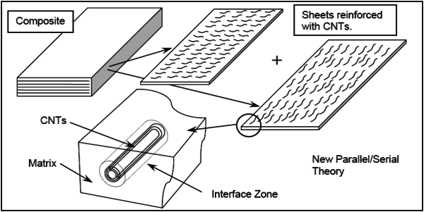
|
| Figure 2: Representation of formation for reinforced composite. |
First, the layer is split into matrix and a new material that results of coupling the CNTs with the interface. The relation between the matrix and the CNT-interface material is established in terms of the parallel mixing theory (they are assumed to have an iso-strain behavior). On the other hand, CNTs and the interface are coupled together with a combination of parallel and serial mixing theories. The serial mixing theory assumes that all components have the same stresses.
Figure 3 shows scheme used to obtain the performance of the CNT-interface material. This is based in the short-fiber model developed by Jayatilaka [13]. According to this model, the load is transferred from the interface to the nanotube at the ends of the reinforcement, through shear stresses. In this region normal stresses in the fiber increase from zero to their maximum value, which is reached in the central part of the reinforcement. In this region there is not load transfer and shear stresses are null. This whole stress transfer scheme can be simplified assuming a CNT-interface performance defined by a serial mixing theory at the ends of the reinforcement and a parallel mixing theory at the center of it.
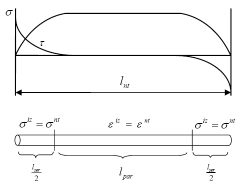
|
| Figure 3: Different regions in the new material CNT-interface. |
A parallel factor named is defined to differentiate these two regions. This parameter, multiplied by the nanotube length, provides the length of the nanotube-interface element with a parallel behavior. The length with a serial performance is defined by the complementary factor.
4.2 Formulation of the composite constitutive model
The Helmholtz free energy [67] of a material point subjected to infinitesimal deformations can be described with the following thermodynamic formulation [16,22]
|
|
(4.1) |
where is the strain tensor, a measure of temperature and a set of inner variables, for example: is the plastic strain tensor, damage inner variable and any other material internal variables.
The proposed model simulates the composite combining the different components using the serial and parallel mixing theories. If this combination is performed according to what has been described in previous Section 4.1, the expression of the Helmholtz free energy may be written as
|
|
(4.2) |
where , and are the specific Helmholtz free energy for the matrix, the nanotube and the interface components, respectively; , and are the volume fraction of each component, is the parallel factor and,
|
|
(4.3) |
are the volume fractions of the carbon nanotubes and the interface in the new CNT-interface material. These volume fractions must verify
|
|
(4.4) |
The relation among the strain tensors of the different components is
|
|
(4.5) |
being and the composite and matrix strain tensor, respectively; the strain tensor of the new CNT-interface material with a parallel behavior; and the strain tensor of the CNT-interface material with a serial behavior.
The tangent constitutive tensor of the composite material may be derived from 4.2 as
|
|
(4.6) |
A parallel behavior means that all composite constituents have the same strain value. Therefore:
|
|
(4.7) |
|
|
(4.8) |
And, a serial behavior means that all composite constituents have the same stress value. Thus:
|
|
(4.9) |
|
|
(4.10) |
Replacing 4.8 and 4.10 in 4.6 it is possible to obtain a simplified expression of the tangent constitutive tensor as
|
|
(4.11) |
The formulation developed require all composite components to fulfill the expression given by 4.1. Therefore, it is possible to use any constitutive law to describe the mechanical performance of the different components.
4.2.1 Definition of the parallel factor
The parallel factor is defined as
|
|
(4.12) |
where is the length of the nanotube and is function of geometry and mechanical properties of the nanotube and the interface. The value of this length can be obtained from the equation of tension distribution in a reinforcement considering perfect bond with the matrix, which is [13]
|
|
(4.13) |
|
|
(4.14) |
where represents the longitudinal positions in the reinforcement, and the subscripts “nt” and “iz” refers to the properties of nanotube and interface zone, respectively. and are the Young's modulus and the shear modulus, and is the thickness material around of the CNTs associated with the interface zone.
Defining , its value can be obtained by finding the position “x” for which the effective modulus obtained from the integration of the tension distribution becomes
|
|
(4.15) |
This procedure provides a value of the parallel length of
|
|
(4.16) |
4.2.2 Definition of the volume fraction of the interface region
Based on the results reported in [66], the interface zone can be considered the region surrounding the carbon nanotube in which an amorphous matrix becomes crystalline. The volume fraction of the interface zone can be obtained as
|
|
(4.17) |
where are the volume fractions of crystalline matrix with and without CNTs, respectively. Assuming that the interface zone is a cylinder around the CNTs, it is possible to relate the volume fraction of the interface zone with the parameter as
|
|
(4.18) |
where is the total composite volume, is the radius of interface zone and is the total number of nanotubes in the composite.
The relation between the radius of the nanotube and the interface is obtained replacing 4.18 in 4.17 as
|
|
(4.19) |
and therefore
|
|
(4.20) |
4.2.3 Equivalent properties for MWCNTs
MWCNTs consist of concentric SWCNTs joined together with relatively weak van der Waals forces. For this reason, the capacity to transfer the load from the external wall to the internal walls is low. Some papers [68,69] propose to simulate the CNTs like a solid cylinder with same exterior diameter and length, but with effective properties. The effective properties are obtained assuming that the outer wall takes the total load. In this approach it is assumed that the properties of the outer wall correspond to those of a graphite sheet. The effective stiffness of the MWCNT is calculated by imposing that for a same applied force, the deformation must be the same
|
|
(4.21) |
where and are the Young's modulus of the effective solid nanotube and graphite sheet, respectively, and and are the areas of the effective solid nanotube and outer wall, respectively. Equation 4.21 can be also read as
|
|
(4.22) |
being the thickness of one wall in the MWCNT and is the external diameter of the MWCNT.
Using the same procedure it is possible to obtain the shear modulus of the solid cylinder, by forcing the same twist when applying the same torque (T).
|
|
(4.23) |
where and are the shear modulus of the effective solid CNTs and graphite sheet, respectively, and and are the polar moment of inertia of the effective solid CNTs and outer wall, respectively. They are
|
|
(4.24) |
Replacing the expressions given by 4.24 in 4.23, the equivalent shear modulus can be written as
|
|
(4.25) |
Finally, it is necessary to obtain the new density of the effective solid CNTs, as the total weight of the MWCNTs can not change in the composite when they are considered a solid cylinder, then
|
|
(4.26) |
being the density of the graphite sheet () and the internal diameter of the MWCNTs.
The most common parameter used to define the amount of CNTs added to a composite is their weight fraction. However, the composite constitutive model developed requires knowing the volume fraction. The volume fraction of CNTs in the composite is the volume that occupies a solid cylinder with the same external diameter. This parameter can be calculated with the following expression [68] as
|
|
(4.27) |
where is the weight fraction and is the density of the matrix.
4.2.4 Material non-linearity of the proposed model
In the proposed model, the composite performance is obtained from the mechanical response of its constituent materials, and each component is simulated with its own constitutive law. Therefore, if a constituent (i.e. the interface) is simulated with a non-linear law, the whole composite will become non-linear. As it has been already explained, with the present model it is possible to use any non-linear formulation to simulate the component behavior, such as plasticity, damage, viscosity, etc.
Besides the non-linear performance provided by each constituent, the load transfer capacity of the interface region is also affected if the interface is damaged. This effect must be included in the formulation.
According to Figure 3, the load is transferred from the interface to the CNTs reinforcement at their ends. Interface damage is expected to occur at the ends of the reinforcement, where there is larger stress concentrations. Assuming that the damaged region is unable to transfer loads and that the length required to transfer loads must remain constant, interface damage ends up affecting the parallel length of the nanotube, which can be calculated as
|
|
(4.28) |
Here, is the initial length of the nanotube working in parallel and is the interface damage inner variable.
The dependence of the parallel length on the interface material damage provides a non-linear response of the composite, even when matrix and the carbon nanotube reinforcement are in their linear range.
4.3 Numerical Implementation
The proposed composite constitutive model has been implemented in PLCd [9], a finite element code that works with 3D solid geometries. The algorithm developed is described in Figure 4. PLCd has already implemented the constitutive laws that will be used to predict the performance of the composite components (elasto-plastic, elasto-damage and elastic). The formulation proposed has been written so that the constitutive laws of the constituents are seen as “black boxes”, following the recommendations of [33] and [4].
The FEM code enters into the new formulation with the prediction of the strain tensor of the composite material in the actual time step. Layers are assumed to have all the same strain; therefore the strain tensor of each layer is obtained rotating the composite strain to the direction in which the CNTs are oriented. In each layer, the strain of the matrix and the CNTs-interface are the same, as they work in parallel, (see 4.5). Knowing the strains for matrix material it is possible to obtain its stresses straightforward. On the other hand, to obtain the stresses for the CNT-interface material, it is necessary to separate it in two regions. In the flow chart shown in Figure 4, these two regions are represented as “Parallel Block” and “Serial Block”. This division is performed based on the value of (defined in 4.12). This value depends on the damage evolution of the interface, as has been explained in section 4.2.4.
The Parallel Block corresponds to the central region, where the CNTs and the interface work in parallel behavior and, therefore, they have the same strains. In this region the stresses for each component are obtained from the strain tensor, using their constitutive equation. Finally, the stress tensor of the CNT-interface material in the “Parallel Block” at time is
|
|
(4.29) |
On the other hand, at the ends of the CNTs, the interface-CNTs material has a serial behavior and it is necessary an initial prediction of the CNT or of the interface strains, in order to integrate the local stress in both components. If this initial prediction is made on the interface, its strains can be computed as
|
|
(4.30) |
|
|
(4.31) |
|
|
(4.32) |
And, the strain tensor of the interface in the iteration step is used to calculate the strain tensor of the CNT as
|
|
(4.33) |
|
|
(4.34) |
Once knowing the strain tensor of both component materials, the constitutive law of each one is used to calculate their stress tensor. Afterwards it is necessary to verify that the iso-stress condition is indeed fulfilled. Therefore
|
|
(4.35) |
If the residual stress is greater than the tolerance, the prediction of the interface strain must be corrected. A Newton-Raphson scheme is adopted to do this correction. The method uses the Jacobian to update the unknown variable, in this case, the interface strain, then
|
|
(4.36) |
and, finally
|
|
(4.37) |
Therefore, the strain tensor of the interface for the next step n+1 is estimated as
|
|
(4.38) |
This iterative process continues until the residual stress is smaller than the required tolerance.
The final stresses in the serial region “Serial Block” of the CNTs-interface are
|
|
(4.39) |
And at the end, the final stress tensor for a specific layer is obtained as
|
|
(4.40) |
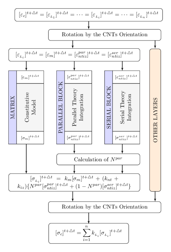
|
| Figure 4: Flow chart of the proposed model in a FEM code. |
5 Validation and numerical results
In this chapter, the validation of the proposed constitutive model using data from the literature is presented. Then, a numerical example is shown using the model calibrated. The basic formulation of the different constitutive models used for the simple materials can be seen in the Appendix A.
5.1 Validation of the elastic response
In the following section are compared the composite stiffness predicted by the composite constitutive model (see Section 4.2) with experimental data obtained from the literature. For this elastic properties validation the experimental data presented in the papers of Coleman et al. [65,70] is used. In these works several composites made of the same matrix with different MWCNTs are experimental tested.
Materials description
In the following, it will present the mechanical properties of the material components used and the composites data.
Matrix component:
The matrix material is polyvinyl alcohol (PVA) and its Young's modulus is given by the authors as [GPa] [65].
Interface component:
The authors found that the Young's modulus of the crystalline polymer phase is of [GPa]. On the other hand, the parameter is estimated following the procedure described in Section 4.2.2.
MWNTs component:
The nanotubes used in [65] are an arc grown MWCNT (Arc-MWCNT), two types of catalytic MWCNT from Nanocyl S.A. (CVD-1, CVD-2), a catalytic MWCNT produced in Orléans (France) (CVD-3), and a double walled nanotube (Dwnt). While in [70] the nanotube used is MWCNT from Nanocyl S.A. (MWCNT).
The maximum Young's modulus of the CNTs is [TPa][65], which corresponds to the stiffness of a perfect graphite sheet. The equivalent stiffness (see Section 4.2.3) of the nanotubes are calculated using this perfect stiffness value and considering a thickness of the outer layer of [nm][34,68].
The most important collected data of the nanotubes used are presented in table 1:
| Type | ||||||
| Arc-MWCNT | 24 | 1 | 42 | 0.81 | 56 | 0.97 |
| CVD-3 | 16 | 3.8 | 238 | 1.47 | 83 | 0.99 |
| CVD-2 | 14 | 2.1 | 150 | 2.27 | 95 | 0.99 |
| CVD-1 | 15 | 1.8 | 120 | 2.83 | 89 | 0.98 |
| Dwnt | 2.5 | 2.2 | 880 | 4.87 | 470 | 0.99 |
| MWCNT | 15 | 1.72 | 115 | 3.30 | 89 | 0.98 |
Composites:
A parameter missing in Table 1 is the direction distributions of the CNT. In general, obtaining this information from the composite is very complicated. To outstep this impediment it is possible to rewrite equation given by 4.11 for one layer as
|
|
(5.1) |
where
|
|
(5.2) |
Cox [71] and Krenchel [72] modified the rule of mixtures proposing the following equation to calculate the composite Young's modulus
|
|
(5.3) |
where and , are the Young's modulus of the matrix and effective reinforcement, respectively. The volume fraction for each component is and is a fiber orientation efficiency factor. For the present validation 5.3 will be modified, adapting it to the developed formulation. Therefore
|
|
(5.4) |
The value of the efficiency factor related to fiber orientation was taken from literature. In composites with a random distribution, .
Results
![Comparison of numerical and experimental results [65,70].](/wd/images/thumb/1/16/Draft_Content_281472310-monograph-05Elastic_Results.png/600px-Draft_Content_281472310-monograph-05Elastic_Results.png)
|
| Figure 5: Comparison of numerical and experimental results [65,70]. |
Figure 5 shows the values of , this is: the slope of the curves of Young's modulus () divided by volume fractions of nanotubes (), for the different composites considered. In the figure the short lines represent the limits of the range experimental results presented in [65,70] and the red points correspond to the numerical result for each CNT type, obtained with the proposed composite model.
This figure shows that the formulation is capable of predicting the elastic stiffness of the composite, as most of the values obtained are comprehended between the limits defined by the experimental tests. There is only one case in which the value obtained exceeds the limits of the experimental test. This is because the effective Young's modulus of the Dwnt is highest since its diameter is really low.
5.2 Validation of the non-linear performance
The non-linear behavior of the composite constitutive model has been validated comparing the results provided by the model with the experimental data obtained from the paper of Meng et al. [73]. In that article the matrix used is Polyamide 6 (PA6) and all composites contained a 1 wt% of MWCNTs reinforcement.
The MWCNTs used in the experimental tests were purchased from Chengdu Organic Chemistry Co. Ltd. Two different composites where manufactured with these nanotubes. One of them contains the nanotubes “as is”, without any previous treatments. These nanotubes are called U-MWCNT. The other composite uses nanotubes that where treated with a mixture of concentrated sulfuric and nitric acids. These are called A-MWCNT.
Materials description
In the following, it will present the properties of the material components used and the information of the composites.
Matrix component:
The matrix material is characterized with an isotropic, elasto-plastic model using a Von-Mises yield criterion. The mechanical parameters of the model were calibrated using the experimental data described in [73], obtaining a Young's modulus of [GPa], a Poisson ratio of and an elastic threshold of 35 [MPa]. The parameters used to simulate matrix material are validated comparing the stress-strain graph obtained with the numerical model with the experimental one. This comparison is shown in Figure 6.
![PA6 stress-strain relations for static tests [73].](/wd/images/thumb/9/9b/Draft_Content_281472310-monograph-06PA6PaperMeng.png/600px-Draft_Content_281472310-monograph-06PA6PaperMeng.png)
|
| Figure 6: PA6 stress-strain relations for static tests [73]. |
Interface component:
The interface zone is associated with the crystalline matrix around of MWCNTs. The properties of this material are better than those of the amorphous matrix. The volume fraction of the interface zone has been estimated with the data presented in the paper of Meng [73] and the equations developed in Section 4.2.2. On the other hand, the mechanical properties of the interface are used to calibrate the model. In current simulation, the interface has been defined with a isotropic, elasto-damage model with linear softening and Tresca yield surface. The mechanical parameters used are [GPa], and [GPa]. Damage in the interface starts for a stress threshold of 120 [MPa]. This value is in the range of theoretical and experimental tests value obtained in [46].
MWCNTs component:
Numerical simulations of molecular structural mechanics of CNTs show that the Young's moduli are in the range of [TPa] and the shear moduli is about [TPa] [74]. It has been also shown that these values do not change significantly for CNTs with two, tree or four walls.
Regarding the transverse modulus of CNTs, it has been assessed from numerical and experimental results that there is an inverse relationship between axial and transverse modulus for carbon fibers [75]. Higher axial stiffness is associated to a longer and more aligned crystalline structure of the nanotube in this direction, which reduces properties in the transverse direction. Following this approach, in current simulation the transverse moduli of the MWCNTs are defined with the same values of the interface component.
Therefore, the equivalent properties of the MWCNTs were obtained using the equations described in Section 4.2.3. The diameter of MWCNT is [nm]. The measurement of several MWCNTs provided an estimation of the internal diameter of [nm] [68]. The effective density of MWCNTs has a value of ; and the volume fraction of MWCNTs in the composite is 0.51 % The MWCNTs have been simulated using an elastic orthotropic material with the following properties:
[GPa] , [GPa]
[GPa] , [GPa]
Composite:
The composites tested had a random distribution of the MWCNTs. This is simulated in the numerical model by dividing the composite in several layers, each one containing CNTs with a different orientation. Current simulation divides the composite in 10 layers and CNTs angles varying from to . Each layer has a volume fraction of 10 % Table 2 shows the volume fractions of the three composite components in each layer. This table also shows some geometry information of the MWCNTs and the interface zone, as well as the initial value of .
| Composite | [% | [% | [% | |||
| PA6/A-MWCNT | 0.5 | 4.1 | 95.4 | 250 | 2.00 | 0.98 |
| PA6/U-MWCNT | 0.5 | 5.3 | 94.2 | 250 | 2.35 | 0.98 |
Results
In Figure 7 are represented the numerical and experimental results obtained for the composite made with A-MWCNTs. This figure shows an initial reduction of the composite stiffness, result of matrix yielding. Afterwards damage begins in the interface zone and, consequently, the composite continues reducing its stiffness. Interface damage leads to a reduction of the parallel length (see 4.28). When the interface is completely damaged, the whole CNT-interface material has a serial performance. At this stage stresses in the interface are zero, and so must be the stresses in the carbon nanotubes. Therefore, the final stiffness of the composite corresponds to a material with a volumetric participation of 95.4 % of PA6 matrix, and the rest of the material correspond to voids.
![PA6/A-MWCNT stress-strain relations for static tests [73].](/wd/images/thumb/d/da/Draft_Content_281472310-monograph-07PA6_AMWNT_PaperMeng.png/600px-Draft_Content_281472310-monograph-07PA6_AMWNT_PaperMeng.png)
|
| Figure 7: PA6/A-MWCNT stress-strain relations for static tests [73]. |
Figure 8 shows the results for the composite made with U-MWCNTs. This composite is the same than the previous one (made with A-MWCNTs), with the only difference that in this case the bond between U-MWCNTs and interface zone is weaker. To take into account this difference, the numerical model used for this composite is the same used for the previous one, varying the threshold at which damage starts in the interface. In current simulation this value is reduced to 70 [MPa].
This simulation provides a maximum stress in the composite lower than the value obtained for previous one, consequence of having a weaker interface. The simulation also shows some divergences between the numerical and the experimental values. Both graphs start to differ for a strain of 2.5 % and the maximum load reached by the numerical simulation is larger than in the experimental tests. However, it has to be noted that the experimental tests provide a maximum stress lower than having just plain matrix (see Figure 6). Therefore, the differences observed in Figure 8 may be justified.
![PA6/U-MWCNT stress-strain relations for static tests [73].](/wd/images/thumb/e/e0/Draft_Content_281472310-monograph-08PA6_UMWNT_PaperMeng.png/600px-Draft_Content_281472310-monograph-08PA6_UMWNT_PaperMeng.png)
|
| Figure 8: PA6/U-MWCNT stress-strain relations for static tests [73]. |
5.3 Simulation of a four points bending beam
5.3.1 Materials properties, geometry and FE model of the analyzed structure
This section presents the numerical simulation of a four points bending beam, which is shown in Figure 12. Although there is no experimental results available to compare the results obtained with the numerical simulations, the analysis performed is used to show the numerical performance of the proposed model and the effect of reinforcing the polymer with CNTs. The validity of the results is assumed, based on the comparisons made in Section 5.1 and 5.2. The composite used in the simulation is a reinforced matrix with MWCNTs and it has been proposed in the framework of M_RECT project. The matrix in the composite is a Polyether Ether Ketone (PEEK) thermoplastic polymer provided by Victrex company. While the MWCNTs are the NanocylNC7000 from Nanocyl S.A. Two composite with different weight fractions percentage (0.5 and 2.0 wt%) of MWCNTs reinforcement will be analyzed.
In the following, it will describe the properties and constitutive model of the material components and the composites information.
5.3.1.1 Matrix component
An elasto-plastic constitutive model with hardening is applied to characterize the behavior of the PEEK component. The matrix material has a Young's modulus of [GPA], a shear modulus of [GPA], a Poisson ratio of . These elastic mechanical properties are obtained from M-RECT project and of the information provided by Victrex(http://www.victrex.com). The constitutive model is calibrated with an elastic threshold of [MPa] and an ultimate tensile strength of [MPa]. Figure 9 shows the comparison between the experimental data from the project and numerical results obtained with the constitutive model calibrated.
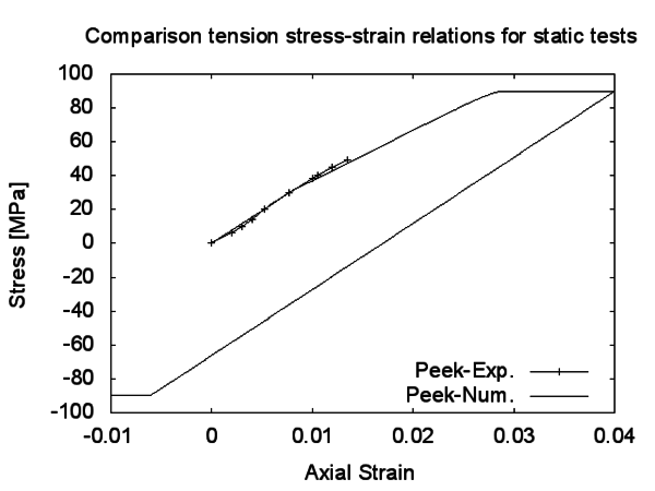
|
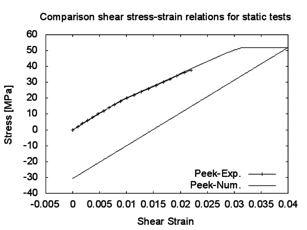
|
| (a) In a tensile test. | (b) In a shear test. |
| Figure 9: Comparison of the experimental data with the numerical results for PEEK. | |
5.3.1.2 Interface component
The constitutive model used to simulate the behavior of the crystalline PEEK around of the MWCNTs is an elasto-damage model with exponential softening. The mechanic properties of this interface zone are obtained following the same procedure used by Coleman et al. [65] but using the information presented in the works of Diez-Pascual et al. [76,77], which use the PEEK material as matrix too. Then, the properties obtained are, a Young's modulus of [GPa], a shear modulus of [GPa] and a Poisson ratio of . The value of the elastic threshold used in the model is of 28 [MPa]. This parameter is obtained when the composite constitutive model is calibrated to reproduce the experimental curve shown in Figure 10. This experimental data is for a PEEK reinforced with 3 wt% of MWCNTs obtained in the framework of the previous referred project.
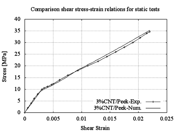
|
| Figure 10: Experimental data and numerical response with the calibrated interface component model. |
5.3.1.3 MWCNTs component
The geometric characteristics of the MWCNTs are obtained from the paper of Jiang et al. [78], who obtains as average diameter and length of [nm] and [m], respectively. For the simulation the MWCNTs are considered as an orthotropic elastic material. The equivalent properties are obtained using the equations described in Section 4.2.3, assuming [TPa] and [TPa][74] and a thickness of the outer layer of [nm][34,68]. And taking the same consideration than before, the transverse properties are defined with the same values of the interface.
[GPa], [GPa],
[GPa], [GPa],
,
.
5.3.1.4 Composites
Table 3 shows the volume fractions of each component in the composites simulated.
| Composite | [% | [% | [% |
| PEEK-0.5CNT | |||
| PEEK-2.0CNT |
The orientation distribution of the MWCNTs has been defined assuming that the composite is formed by several layers, each one with a specific angle and volume fraction of MWCNTs. The volume fractions of the MWCNTs for the different layer in the composite are shown in the Figure 11. The value of the volume fractions in the figure are relative values respect to the total volume fraction of the MWCNTs in the composite.
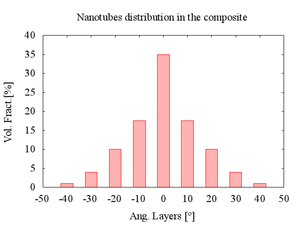
|
| Figure 11: MWCNTs orientation distribution in the composite. |
5.3.1.5 Geometry of the simulated structure
The selected structure for the numerical simulations is a simple supported beam with two concentrated loads, which are applied at of both beam ends. Figure 12 shows the geometry and its dimensions, the boundary conditions and the load position on the analyzed structure.

|
| Figure 12: Geometry and extra information of the analyzed structure. |
5.3.1.6 FE model used
The symmetry of the geometry, of the applied load and of the boundary conditions of the structure allows to reduce the numerical model in the simulation. For this case, the reduced FE model is a quarter of the real geometry of the structure. Figure 13 shows the numerical model and the FE mesh used for the numerical analysis. The more relevant data about the FE mesh is shown in the Table 4.
| Item | Nodes | Elements | Type Elem. | Order |
| Quantity/Type | 1953 | 1200 | Hexahedron | Quadratic |
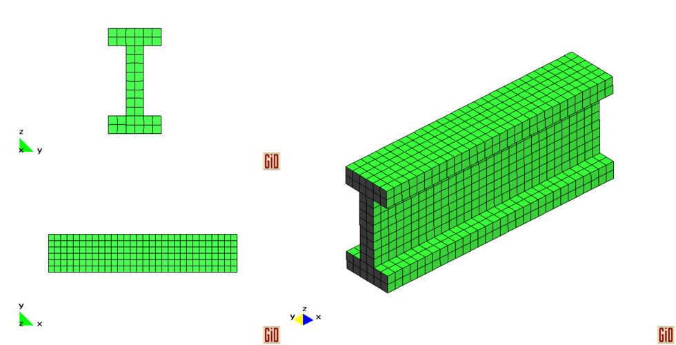
|
| Figure 13: FE mesh used in the reduce model. |
In order to obtain the real behavior of the structure with the reduced FE model it is necessary impose the restrictions on the numerical model given by the symmetry. There are two symmetry planes: The X-axis symmetry plane that has as normal axis the longitudinal axis (X-axis). In this symmetry plane, X direction displacements on the plane's nodes are restricted to zero. The other symmetry plane is the Y-axis symmetry plate, which has as normal axis the Y-axis in the model. For this symmetry plane, the null displacements restriction on the plane's nodes is Y direction. The longitudinal direction in the numerical model (X-axis) is taking as a reference direction for the definition of the layes' angle in the composite.
5.3.2 Linear analysis
The numerical results obtained in the simulation are presented in comparative form, taking as reference the result obtained for the non-reinforced matrix (plain PEEK material).
In all cases, the applied load for elastic analysis is a fixed displacement of a [mm] in Z direction at P position (see the Figure 12). The result considered for the comparison is the reaction force in Z direction on the support. As the imposed displacement is the same for all analysis, the reaction force increases when the material is the PEEK reinforced. Table 5 shows the results obtained for the different composites normalized by the non-reinforced PEEK results.
| PEEK | PEEK-0.5%CNT | PEEK-2.0%CNT |
| 1 | 1.20 | 1.52 |
In the central section of the beam, between concentrated loads, there is a pure bending situation. While, at both ends of the beam there are a coupling bending and shear conditions. In Table 6, it is possible to observe the longitudinal (X direction) and shear (XZ direction) stresses obtained in the structure with the different composites.
| Longitudinal Stress | Shear Stress | |
| PEEK | 
|
|
| PEEK-0.5%CNT | 
|
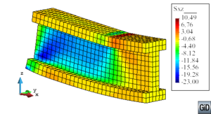
|
| PEEK-2.0%CNT | 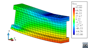
|
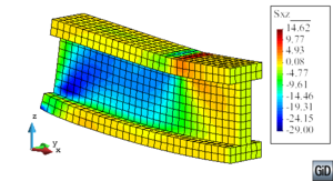
|
5.3.3 Non-linear analysis
In order to obtain the non-linear response of the structure the fixed displacement at P position is gradually increased in the simulation. Therefore, the reaction force in the support in Z direction increases too until the maximum value that the structure is able to take. The total force is four times the value obtained from the numerical model because the symmetry. The vertical (Z direction) displacement at the middle of the beam is taking as the reference loading increase.
The fixed displacement is applied to the numerical model in load steps of [mm]. Figure 14 shows the results obtained in the simulation for the different composites. When the vertical displacement is around [mm] the curves show the first loss of stiffness. This is because in the middle of the beam starts the plasticity in the PEEK. Then, when the vertical deformation is between [mm] to [mm] there is the second loss of stiffness. In this case, it is due to the damage in the interface zone. Subsequently, it is possible to observe that the model with non-reinforced PEEK has a higher stiffness than the ones with MWCNTs. This strange phenomenon is because at this point of the simulation the interface zone is completely damaged and, therefore, the contribution of the MWCNTs to the global stiffness is null. The stiffness obtained with the composites with MWCNTs are equivalent to the stiffness of a plain PEEK material but with some holes. This effect is clearly observed in Figure 15. This Figure shows the curves obtained for the simulation until a vertical displacement of [mm].
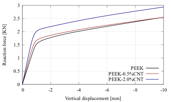
|
| Figure 14: No-linear structural response for PEEK-CNT. |
Figure 15 shows a new loss of stiffness that takes place from [mm] to [mm] of vertical displacement. This laster loss of stiffness is because the plasticity model in the PEEK arrives to the ultimate tensile strength in the middle zone of the beam.
![No-linear structural response for PEEK-CNT up to 50 [mm] of vertical displacement.](/wd/images/thumb/b/bf/Draft_Content_281472310-monograph-ForcevsDispl_2.png/600px-Draft_Content_281472310-monograph-ForcevsDispl_2.png)
|
| Figure 15: No-linear structural response for PEEK-CNT up to [mm] of vertical displacement. |
Figure 16a shows the distribution of the longitudinal stress and Figure 16b of the shear stress for the composite reinforced with 0.5% of MWCNTs for a vertical displacement of 1 [mm]. The longitudinal plastic strain for the same composite and displacement state is shown in Figure 16c and the equivalent stress in Figure 16d.
5.3.4 Visco-elastic analysis
One of the main improvements shown by CNTs reinforced composites is their good damping response and energy dissipation, which makes them very useful for impact or vibration absorption purposes [69,79,80]. For this reason, in the following is analyzed the visco-elastic performance of the numerical model developed under such conditions. In order to obtain a viscous response of the composite it is necessary to use a visco-elastic model to characterize its components. The visco-elastic model used for the matrix and the interface zone is the generalized Maxwell model (see Figure 17) [3], which is already implemented in the PLCd code (see Section A.4 in Appendix A). To conduct the visco-elastic analysis, the MWCNTs are considered to have a linear elastic behavior.
![Scheme of the generalized visco-elastic Maxwell model [3].](/wd/images/f/f8/Draft_Content_281472310-monograph-Viscomodel.png)
|
| Figure 17: Scheme of the generalized visco-elastic Maxwell model [3]. |
| Mat./Prop. | [MPa] | [MPa] | [MPa.seg] |
| PEEK | 3900 | 390 | 39 |
| Interface | 5070 | 1521 | 152 |
The response obtained, after calibrating the model (see Table 7), is shown in Figure 18. This figure shows the stress-strain curve of a point inside of the structure in a complete sinusoidal load-unload cycle. The numerical simulation has been conducted using the two composites previously described (0.5% and 2.0% wt) and the plain PEEK. Figure 18 shows that the areas enclosed by the curve, in the load-unload cycle, in the composites reinforced with MWCNTs are larger than the non-reinforced matrix (plain PEEK). In other words, the dissipation capacity of a composite with MWCNTs is better than the matrix alone. The composite reinforced with 0.5% wt of MWCNTs has higher dissipative capacity than the other composite (2.0% wt). This is because, in this composite, the volume fraction of the interface zone is higher than in the other, as it is shown in Table 3. This phenomenon occurs because when the volume fraction of the MWCNTs in the composite is low, their distribution in the composite improves, and then, increasing the interface volume.
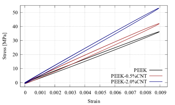
|
| Figure 18: Structural response for a sinusoidal load-unload of 1 Hz. |
5.4 Effect of the CNTs angle on the elastic properties
The present study about the influence of the CNTs angle in the resulting elastic properties using the developed composite constitutive model has been performed to asses the importance of having a good orientation of the CNTs in the composite.
The composite used for the analysis is a CNTs reinforced PEEK matrix and it has been also proposed in the framework of M_RECT project. The PEEK material used as matrix in the composite is the same than the one used in the above section (see Section 5.3.1). Therefore, the elastic properties previously obtained for the matrix and interface components have been used in this study. However, the MWCNTs used as reinforcements in the composite are the Baytubes C70P from Bayer, which have different geometric characteristics than the ones used in the above section. The current CNTs have an average diameter and length of [nm] and [m], respectively. The CNTs are considered as an orthotropic elastic material and the equivalent properties are obtained using the equations described in Section 4.2.3, assuming [TPa] and [TPa][74] and a thickness of the outer layer of [nm][34,68]. Considering that the transverse properties are defined with the same values of the interface, the CNTs properties are
[GPa], [GPa],
[GPa], [GPa],
,
.
The composite simulated in the analysis has a 3% weight of CNTs, which represent a 1.94% of volume fraction. However, measurements made with X-rays show an apparent 5% weight. This difference is obtained because the MWCNTs have a higher apparent diameter than the original one. Therefore, the parameter is estimated assuming that this extra 2% weight in the measurement is the coating polymer around the nanotubes and then, it is the interface component considered. Taking this into account, the interface component has an approximate volume fraction of 1.31% and .
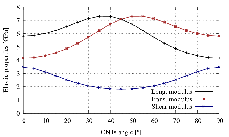
|
| Figure 19: Change of elastic properties of CNTs reinforced PEEK with the CNTs angle. |
Figure 19 shows the variation in the longitudinal elastic modulus, the transversal elastic modulus and the shear elastic modulus in the composite obtained when the CNTs angle is changed. The curves obtained, which are shown in the figure are symmetric with respect to the 45º vertical line. This behavior is different to the typical ones expected for reinforced matrices. In general, the maximum value of the longitudinal Young's modulus in the composite is obtained when the angle of the reinforcement is equal to 0º. For this reinforced PEEK with CNTs, the longitudinal Young's modulus increases from 0º until 40º and then, it decreases until its minimum value, which is obtained for an angle of 90º. A similar behavior presents the transversal Young's modulus but symmetrically respect to the 45º vertical line. The maximum value for the shear modulus is presented for an angle of 0º and the minimum for 45º.
6 Phenomenological homogenization. Concluding remarks
A new phenomenological composite constitutive model, based on the mixing theory, capable of predicting the mechanical performance of composites reinforced with carbon nanotubes has been presented. The formulation presented relates the reinforcement and the matrix in which they are embedded, using an interface material. This approach makes possible to consider non-linear phenomenons, such as debonding, by using non-linear constitutive laws to characterize the interface material. The formulation is written in a way in which all materials can be defined with their own constitutive law, improving the versatility of the model.
It has been shown that the elastic properties estimated with the model are in good agreement with experimental values obtained from literature. Only the numerical model of the composite made with the Dwnt reinforcement has given results in which the composite stiffness is overestimated. This is because the Dwnt has a very small diameter, which leads to a very high value of its equivalent Young's modulus.
The validation of the non-linear response provided by the proposed composite model has been performed using the experimental data of two different composites made with MWCNTs randomly distributed. The numerical curve obtained for the A-MWCNT is in good agreement with the experimental results. On the other hand, the numerical prediction obtained for the U-MWCNTs differs from the experimental results for strains larger than 2.5% However, it has to be said that the experimental results are lower than expected, as this composite is weaker than plain matrix.
Then, the formulation has used to predict and compare the mechanical properties of a straight beam subjected to four-point bending, with different material configurations. A non-linear analysis has also been made using the same structure and composites. The non-linear response of the beam obtained from the numerical simulation shows different points where there is a loss of structural stiffness. This structural behavior is obtained because the component materials in the composite reach their elastic thresholds and ultimate strength.
A visco-elastic material constitutive model is used for the polymeric matrix and the interface zone. The viscous response within the elastic range of the materials has been studied. The good capacity of energy dissipation in composites reinforced with MWCNTs has been proved with the simulations performed.
Finally, the composite constitutive model has been used to analyze the effect of nanotube orientation in the elastic properties of the composite, showing that the CNTs distribution within the reinforced matrix has a meaningful influence on the composite properties achieved.
All these tests have proved the validity of using a phenomenological model for the characterization of these materials. The developed composite constitutive model allows an accurate characterization of this kind of composites with an affordable computational cost, moreover taking into account the scale size of these reinforcements.
Part II. Multiscale homogenization
7 Introduction
In the last decades, several formulations have been developed to mathematically characterize and model composites as heterogeneous materials. Large number of composite models have been proposed to assess the global behavior of these materials by fulfilling the thermodynamic laws in linear and non-linear range. Constitutive equations have been developed for composites with different arrangements such as materials with long and short fibers, nanofibers, fibers laminated with one or more directions, and even random reinforcement distributions, etc. However, these formulations are limited because the constitutive relationships were made on a particular composite material and in general, can not be extrapolated to other composites.
The homogenization methods analyze the composite materials from an internal structure point of view. Over the years, many techniques have been developed, among them: the effective medium approach [81]; the self-consistent method [82]; the variational boundary method, which provides upper and lower limits of the total stiffness [83,84]; and the asymptotic homogenization method [85,86]. Due to the complex task that is required to represent the microscopic mechanical behavior of composites, homogenization approaches that use the RVE concept, together with stable computational methods, are very convenient in most cases. The behavior of the whole composite is obtained by a micromechanical study of the material components and their interaction within of the composite's microstructure through an RVE model.
Within the context of the homogenization methods, the known multiscale techniques use the RVE concept to address the characterization of composites and structures. As a result, these multiscale procedures do not obtain a closed form for the general constitutive equations. The stress-strain relationship of the composite is obtained by performing a detailed modeling of the its microstructure at the micro-scale in the RVE model. Among the main advantages of these techniques it is found that: they do not require any composite constitute assumption at the macro-scale; they can use any constitutive law in the simple materials, even non-linear response and time-dependency; and they can employ many computational techniques to find the response at the micro-scale, such as, the FEM, the Voronoi cell method, or numerical methods based on the fast Fourier transforms, etc.
The first-order homogenization [6] is one of the most extended and popular multiscale methods used nowadays. The approach uses the macro-scale deformation gradient tensor (or the strain tensor) to solve the micro-scale problem and then, by means of the microscopic results obtain the macro-scale stress tensor. The microscopic problem is solved through a Boundary Value Problem (BVP) on the RVE with particular boundary conditions, which are obtained using the macroscopic input. The resolution of the micro-scale BVP can be obtained through any mathematical or numerical approaches. After the solution of microstructural BVP, the microscopic displacement, deformation and stress fields are found and then, the macroscopic stress tensor is calculated as the volume average of the microscopic stress field. The BVP on the macro structure can be also approached through mathematical or numerical methods. When the solution of the coupled macro-micro BVPs is faced by FEM at both scales the formulation/implementation is called homogenization [7].
The advantages above described of the multiscale techniques become a challenge when a non-linear analysis is made on a realistic three-dimensional structure using a homogenization approach. In general, the required computational cost is extremely expensive for non-linear simulations because they require to solve, for each integration point at the macro-scale, one RVE at each time step of the analysis. Furthermore, from an energetic point of view the method must be consistent and therefore, the conservation of the dissipated energy through the scales should be guaranteed.
In the last decade, a second-order computational approach was proposed to be applied in critical regions of intense deformation, where the characteristic wave length of the macro-scale deformation field is of the order of the size of the micro-scale [8]. The homogenization technique has been developed as a natural extension of the first-order homogenization method. In the approach, the macroscopic gradient of the deformation gradient is also incorporated in the microscopic BVP and them, the stress tensor and a second-order stress tensor are retrieved. In the micro-scale level a first-order equilibrium problem is conserved but extra boundary conditions in the BVP must be verified. However, a full second gradient continuum theory appears in the macro-scale level, which requires solving a higher-order equilibrium problem. The solution of the reformulated macroscopic BVP is made through a complex finite element implementation, which has restricted its massive application.
The use of a second-order approach for the non-linear analysis of structures has the advantage of including higher-order effects on the micro-scale. Nevertheless, the complex computational implementation required to solve the macro-scale BVP restricts its application to realistic composite structures. From a mathematical and computational point of view the first-order approach is simpler than the second-order scheme. Then, it would be interesting to develop an enhanced-first-order approach which retains the easy computational implementation but with an enriched solution in the micro-scale.
7.1 Part's outline
In this second part of the present monograph a multiscale homogenization model for composite structures is addressed. The proposed formulation can simulate the behavior of three-dimensional structures in non-linear range.
Following this objective, in Chapter 8 a review of the state of the art of the more relevant homogenization theories is shown. The asymptotic homogenization theory introduces the concept of two or more scale lengths, therefore it lays the foundations of what is today known as multiscale homogenization using RVE concept. At the end of the chapter a review of the most important multiscale approaches found in the literature is made.
Chapter 9 presents the formulation of the two-scale homogenization developed in this study. In the beginning, the first-order homogenization approach is described and then, using concepts of the second-order approach, a enhanced-first-order homogenization is proposed. The BVPs in both scales and their computational implementation through of an efficient three-dimensional FEM is also shown.
In Chapter 10 the results obtained with the first-order homogenization proposed are validated with other microscopic formulations. From the comparison made, it can be observed that the multiscale formulation obtains a good characterization of the composite without any special consideration because the microstructure is modeled using an RVE. The computational run times and memory used are also compared showing the advantages and drawbacks of the proposed method.
Chapter 11 presents a novel strategy for the non-linear simulation of composite structures using multiscale homogenization approaches. This strategy is capable of reducing a 98% the computational time required in a non-linear analysis. The formulation is implemented in the FE code PLCd showing mesh independent at both scales as the develop approach conserves the energy through the scales.
Finally, in Chapter 12 the conclusions of the formulations presented in this part of the monograph are addressed in detail.
8 State of the art
The modeling of heterogeneous composite materials have a high degree of complexity because their constitutive behavior is strongly dependent on microstructural effects. The development of formulations based on multiple scales, capable of predicting the response of a heterogeneous material phenomenologically according to the information derived from a study at the micro-mechanical, is a natural choice to address the problem.
Numerous efforts have been made to mathematically model composite materials and structures with homogenization methods by using suitable multiscale techniques with relatively good approximation to the real global response of the composite. The most significant multiscale techniques, based in different theoretical principles, are:
8.1 The effective medium approximation
The method proposed originally by Eshelby [81] consists to find the current stresses in an elastic solid when a region of it, normally called inclusion (see Figure 20), suffers a change of shape and size which, if the surrounding material was absent, is represented by a uniform homogeneous deformation. By means of the Eshelby solution a number of very important boundary value problems can be solved, like: i) the solution for an ellipsoidal inclusion embedded within an elastically mismatched matrix, ii) the solution for an ellipsoidal cavity in an elastic solid and iii) the solutions for circular and elliptical cracks in an elastic solid. Moreover, several theories which estimate the elastic properties of composite materials use the Eshelby solution. Further developments by Hashin [87], obtain expressions for the elastic moduli and their values bounds of many-phase heterogeneous materials using an approximate method based on the variational theorems of the elasticity theory and on a concentric-spheres model. Besides, Mori and Tanaka [88] developed a method of calculating the average internal stress in the matrix of a material containing inclusions with transformation strain. The obtained actual stress in the matrix is the average stress plus the locally fluctuating stress, the average of which vanishes in the matrix. The developed method also shows that the average stress in the matrix is uniform throughout the material and independent of the position of the domain where the average treatment is carried out.
![Ellipsoidal region of the Eshelby inclusion [149].](/wd/images/thumb/2/28/Draft_Content_281472310-monograph-Eshelby_Inclusion.png/450px-Draft_Content_281472310-monograph-Eshelby_Inclusion.png)
|
| Figure 20: Ellipsoidal region of the Eshelby inclusion [149]. |
8.2 The self-consistent method
It may be considered as an extension of the effective medium approximation. The method is proposed by Hill [82] and it uses similar concepts to the Hershey-Kröner theory of crystalline aggregates. The macroscopic elastic moduli of two-phase composites taking into account the inhomogeneity of stress and strain fields are estimated. It is required phases with the character of matrix and of effectively ellipsoidal inclusions, but they can have any concentrations in the composite. The model of three phases or generalized self-consistent model given by Christensen and Lo [89] is a more elaborate version. The method embeds the spherical (or cylindrical fibers) in a cap (spherical or cylindrical) which represents the elastic properties of the matrix. Then, this set is embedded in an infinite medium with the effective properties of the composite material to be determined. Finally, the effective elastic shear modulus of the material is obtained integrating the differential equations governing the behavior of the three-phase boundary conditions and of the applied loads.
A more recent work by Mercier and Molinari [90], which is based on the interaction law (postulated by Molinari [91] and validated by Mercier et al. [92] on the Eshelby problem) proposed two self-consistent schemes for perfectly disordered materials. The first one is valid for any non-linear behavior, and the second scheme is used to aggregates with phases having the same strain rate sensitivity. Both schemes predict accurately the overall response of the composite material and they are able to capture the strain and stress histories of the components too.
8.3 Bounding methods
The bounding methods provide the lower and upper limits to the total stiffness of the system or of the composites. In general, these methods obtain a simpler expressions for the effective elastic properties through the minimum potential and complementary energies. The most relevant of those are:
8.3.1 The classical bounds of Voigt and Reuss
The Voigt approach determines the elastic moduli by averaging stresses, expressed in terms of strains. The method assumes strain uniformity throughout the composite material. Therefore, the average strain of each phase is equal to the applied strain in the composite, which is similar to the rule of mixture assumption. Hence, considering that each component is linear-elastic, the following relationship can be obtained
|
|
(8.1) |
where is the effective elastic tensor of the composite, and are the elastic constitutive tensor and the volume fraction of the phase, respectively.
On the other hand, Reuss proposed to determine the elastic moduli by averaging strains, expressed in terms of stresses but assuming stress uniformity and then all components have the same stress. Therefore, the following estimation for the effective elastic tensor of the composite is obtained as
|
|
(8.2) |
The Voigt and Reuss methods give an upper and lower bounds for the elastic moduli of a composite with an arbitrary random micro geometry. The Voigt approach gives the upper bound of the elastic moduli for the compound material, while the Reuss approach gives the lower bound. These bounding methods depend only of the phase volume fractions, and of course of the elastic constitutive tensors of the components, but do not require any further information or assumption in respect of the microstructure. The expressions obtained for the bounding effective moduli are valid even for anisotropic component materials
8.3.2 The variational bounding method
The authors Hashin and Shtrikman [83] use the variational formulation to obtained the upper and lower bounds for the effective elastic moduli of quasi-isotropic and quasi-homogeneous multiphase materials of arbitrary phase geometry. The obtained bounds are close enough to provide a good estimate to the effective moduli when the ratios between the different phase moduli are not too large. The method obtains analytical expressions for the elastic constants of a heterogeneous material with random isotropic distribution of phases. Later, Walpole [93,94] generalized the bounding method of Hashin and Shtrikman for materials with several phases, which may be arbitrarily anisotropic.
A variational method for bounding the effective properties of nonlinear composite materials with isotropic components with full variational principle status was proposed by Ponte Castañeda [84]. The author proposed two dual versions of the new variational principle and it is demonstrated their equivalence to each other and to the classical variational principles. The approaches are used to determine the bounds and to estimate the effective energy functions of nonlinear composites in the context of the deformation theory of plasticity. For completely anisotropic composites simpler forms of the classical bounds of Voigt and Reuss are recovered from the new variational principles. Also, for isotropic, particle-reinforced composites, as well as for transversely isotropic, fiber-reinforced composites simpler forms for nonlinear Hashin-Shtrikman bounds are obtained.
Lahellec and Suquet [95] proposed a new method for determining the overall behavior of composite materials which can be composed by nonlinear inelastic components. The evolution equations describing the constitutive behavior of the components can be reduced to the minimization of an incremental energy function by using an implicit time-discretization scheme. The alternative minimization problem is rigorously equivalent to a nonlinear thermoelastic problem with a transformation strain which is a nonuniform field. Comparisons with full-field simulations show that the present model is good as long as the variational procedure is accurate in the purely dissipative setting, when elastic deformations are neglected. If this is the case, the model accounts in a very satisfactory manner for the coupling between reversible and irreversible effects and is therefore an accurate model for treating nonlinear viscoelastic and elasto-viscoplastic materials. Lahellec and Suquet [96] in a second part, of the described work, proposed a proper modification of the second-order procedure of Ponte Castañeda and leads to replacing, at each time-step, the actual nonlinear viscoelastic composite by a linear viscoelastic one. The linearized problem is even further simplified by using an effective internal variable in each individual component. The resulting predictions are in good agreement with exact results and improve the predictions of the previous work. The analytical models presented in the previous sections are reasonably able to predict equivalent material properties for relatively simple geometries and low volume fraction of the second component inclusions. But they are, in general, incapable to obtain the evolution of stresses and strains in the microstructure. Moreover, the actual heterogeneous materials cannot be treated with these models because normally these composites have an arbitrary microstructural morphology.
8.4 The asymptotic homogenization theory
This theory has proven to be a powerful technique for the analysis of structural arrangements of two or more scale lengths. Through the use of asymptotic expansions of the displacement and stress fields, and appropriate variational principles, the homogenization methods can provide not only the effective (homogenized) material parameters, but also distributions of stresses and strains at the two levels. Bensoussan et al. [85] proposed an asymptotic expansion of the solution in terms of a parameter , which is the ratio of the period of the structure to a typical length in the domain. The link from the microscopic to the macroscopic description of the behavior of the system is given by solving the problem in two scales defined by the spatial variables and , where is a macroscopic quantity and is a microscopic quantity; is associated with the small length scale of the inclusions or heterogeneities. The asymptotic problem is formulated in mathematical terms as a family of partial differential operators, depending on the small parameter . The operators may be time independent or time dependent, steady or of evolution type, linear or nonlinear, etc. The coefficients of the operators are periodic functions in all or in some variables with periods proportional to . Since is assumed to be small, it is has a family of operators with rapidly oscillation coefficients. The standard classical formulation of this theory is found in the work of Sanchez-Palencia [86,97]. The two-scale process introduced in the partial differential equations of the problem produces equations in , in and in both variables. Normally, the equations in are solvable if the microscopic structure is periodic, and this leads to deduction of the macroscopic equations for the global behavior in . It is emphasized that the homogenized coefficients depend on the local structure of the medium. Fish et al. [98] presented a generalization of the mathematical homogenization method based on double-scale asymptotic expansion to account for damage effects in heterogeneous media. A closed-form expression relating local fields to the overall strain and damage is derived. Non-local damage theory is developed by introducing the concept of non-local phase fields (stress, strain, free energy density, damage release rate, etc.) in a manner analogous to that currently practiced in concrete. Numerical results of the model were found to be in good agreement with experimental data.
8.5 Homogenization using the RVE concept
The multiscale homogenization based on the use of a unit cell or RVE has emerged as one of the most promising methods to compute the response of composite structures. The unit cell is defined as a microscopic subregion that is representative of the entire microstructure in an average sense. The RVE is employed to obtain the effective properties for the homogenized material because it is assumed that it must contain a sufficient number of heterogeneities.
A thorough examination of the several representative volume element definitions found in the literature can be consulted in the review made by Gitman [99]. Moreover, Ostoja-Starzewki [100] points out that the RVE is very clearly defined in two situations only: i) unit cell in a periodic microstructure, as shown Figure 21a and ii) volume containing a very large (mathematically infinite) set of sub-scale elements, possessing statistically homogeneous and ergodic properties as shown Figure 21b.
![Representative volume element models: (a) unit cell approach; (b) statistical and ergodic approach [149].](/wd/images/9/90/Draft_Content_281472310-monograph-rve.png)
|
| Figure 21: Representative volume element models: (a) unit cell approach; (b) statistical and ergodic approach [149]. |
On the other hand, Suquet [6] gives the basic principles of homogenization to obtain the constitutive equations for homogenized properties of a heterogeneous material. The process is resumed in the following three-step scheme and in Figure 22.
- Definition of a representative volume element. The size of this should be large enough to contain a sufficient number of micro heterogeneities of which the constitutive behavior on these individual constituents is assumed to be known.
- Microscopic boundary conditions are obtained based on the macroscopic input variables (e.g. strain tensor), taking into account the geometry, constitutive laws, etc.
- Macroscopic output variables are obtained based on the solution of the microscopic behavior of the RVE. Macroscopic properties of the equivalent homogeneous medium are evaluated.
![Representative homogenization scheme [149].](/wd/images/thumb/9/9d/Draft_Content_281472310-monograph-macromicro.png/1130px-Draft_Content_281472310-monograph-macromicro.png)
|
| Figure 22: Representative homogenization scheme [149]. |
Terada et al. [101] conducted a study for multiscale homogenization of the convergence of the overall material properties when the unit cell size is increased. For general heterogeneous media that reveal irregular material distribution in a micro scale, the study showed that the periodic boundary condition provides the most reasonable estimates among the class of possible boundary conditions for statistical homogeneous media. The work demonstrated that it is not strictly required the periodicity of RVE geometry in evaluating the effective properties. Moreover, at non-linear range the mechanical behaviors are more sensitive to the size of RVE than those of linear case. The authors concluded that with more accurate geometric models of the RVE, and with larger RVE regions analyzed, the analysis provides a better understanding of the actual phenomena in the microscopic region, as well as a better characterization of the overall mechanical material performance.
8.5.1 Multiscale computational homogenization
Renard and Marmonier [102] were the first to use a finite element discretization to model heterogeneous materials with a multiscale approach. The method consists in solving two finite element problems, one for each scale. In the micro scale the geometry of the RVE is meshed and homogenization rules are used to link this with the macro scale problem.
Guedes and Kikuchi [103] studied the mechanical behavior of linear elastic 2D and 3D composite materials through the homogenization method. This study was one of the first that used homogenization in three dimensions. The method was implemented via a finite element technique to analyze a composite with a periodic microstructure. The implementation enabled the calculation of homogenized material mechanical properties, these characterized the overall behavior of the composite, as well as the analysis of the local performance of the material, as it enables the computation of local stress and strain distribution within the microstructure of the composite. An adaptive finite element method was introduced in order to improve the accuracy of the numerical results. An error measure is suggested for the homogenized material constants, based on the a priori error estimations and the numerical implementation.
8.5.1.1 Non-linearity and FE2 homogenization
Swan [104] presented a computational stress and strain controlled homogenization methods for inelastic periodic composites within the framework of displacement finite element. The implementation of the stress controlled method employs a penalty formulation to insure that the displacement solution satisfies the linear-periodic decomposition. The methods were assessed on a complete set of homogenization computations for an elasto-plastic composite, the strain-controlled method was easier to implement and was demonstrated that it has more computationally efficient than the others.
Later, Smit et al. [7] presented a homogenization method for large deformations and viscoelastic material behavior on microscopic and macroscopic level. The homogenization method was implemented in a multi-level two dimensional finite element program with meshes on macroscopic level (mesh of entire structure) and microscopic level (meshes of RVEs). The local macroscopic stress is obtained by applying the local macroscopic deformation on a unique RVE through imposing appropriate boundary conditions and averaging the resulting stress field. To each macroscopic integration point a unique discretized RVE is assigned that provides the local macroscopic stress tensor and the tangential stiffness matrix. A separate iterative finite element procedures on the RVE is used in each iteration cycle of each macroscopic increment. The following Figure 23 shows the proposed scheme by the authors. The computational cost was the main disadvantage of this implementation. The increase in computational time with respect to a single-scale analysis on the same macroscopic mesh was of 160 times for the structure analyzed.
![Schematic representation of a multiscale finite element program [7].](/wd/images/thumb/0/0f/Draft_Content_281472310-monograph-smit_scheme.png/1438px-Draft_Content_281472310-monograph-smit_scheme.png)
|
| Figure 23: Schematic representation of a multiscale finite element program [7]. |
Michel et al. [105] presented a review of several problems which are specific of composites with periodic microstructure composed of linear or non-linear constituents. The study obtains the estimation of phenomenological macroscopic constitutive models through the analysis of a microscopic representative volume element proposing the concept of “macroscopic degrees of freedom”. A general framework permitting either a strain or stress control was proposed, and the implementation of different types of boundary conditions was presented.
Haj-Ali and Muliana [106] proposed a three dimensional micromechanical modeling approach for the non-linear viscoelastic behavior of pultruded composites. A sub-laminate model is used to provide for a nonlinear equivalent continuum of a layered medium. The system is idealized using a weighted-average response of two simplified micromodels with fiber and matrix. The proposed micromechanical framework was able to generate the effective anisotropic non-linear viscoelastic response as a direct outcome of the micromechanical homogenization subcell. The same authors [107] extended the method to an integrated micromechanical and structural framework for the non-linear viscoelastic analysis of laminated composite materials and structures. The micromechanical model is numerically implemented within a shell-based non-linear finite element by imposing a plane stress constraint on its 3D formulation. The micromechanical model provides the effective non-linear constitutive behavior for each Gauss point. The formulation was validated with several experimental creep tests available in the literature. Finally, the work presents examples for non-linear viscoelastic structures, like a laminated panel and a composite ring. In a latter work, Haj-Ali et al. [108] extend the above described method for the analysis of thick-section fiber reinforced plastic (FRP) composite materials and structures. The proposed modeling framework is applied to a pultruded composite system. Non-linear 3D micromechanical models representing the different composite layers are used to generate through-thickness composite's effective responses. The nested non-linear micromechanical models are implemented at each integration point in the finite element structural analysis. The results obtained demonstrated good prediction capabilities for effective properties and for multi-axial non-linear behavior of pultruded composites.
Matsui et al. [109] made a feasibility study and introduced a parallel algorithm to achieve the computational efficiency. The focus was to the inhomogeneous deformation of the overall structure, which may imply the loss of periodicity assumed in the initial state. The study presented an efficient algorithm for the deconcentration of computational loads by using a PC-cluster system. A simple numerical example for three dimensional heterogeneous structure was made. The authors concluded that the two-scale analysis is still expensive, even if a PC-cluster system for parallel computations is available at non-linear range.
Ladeveze et al. [110,111] proposed a mixed, multilevel domain decomposition method or more accurately, as a “structure decomposition” method. The multiscale computational strategy consists of describing the structure as an assembly of simple components: substructures and interfaces. Each of these entities has its own variables and equations. The distinction between the micro and macro levels is made only at the interfaces, where forces and displacements are split into macro contributions and micro complements. A substructure is subjected to the action of its environment (the neighboring interfaces) defined by the force and a velocity distribution on its boundary. An interface between two substructures transfers both the velocity and the force distributions.
Oller et al. [112] extended the work presented by Zalamea [113], with a two-scale numerical homogenization method that assumes the periodicity of the internal structure of the material to address the problem of the steep gradient in the macroscopic field. To prevent the steep gradient in the macroscopic field variables, which is produced by local boundary effects, the authors proposed a local refinement of the finite element mesh. The objective was to maintain the periodic condition on the boundaries of the cells near to the perturbation.
De Souza Neto and Feijoo [114] discussed some equivalence relationships for large strain multiscale solid constitutive models based on the volume averaging of the microscopic stress and deformation gradient fields over a representative volume element. The work established that the volume averaging of the first Piola-Kirchhoff stress over the reference configuration of an RVE is mechanically equivalent to the spatial averaging of Cauchy stress over the deformed RVE configuration. Whenever such conditions are met, multiscale constitutive models resulting from either the reference or spatial stress averaging are identical.
8.5.1.2 High-order multiscale homogenization
The multiscale methods mentioned in the above sections are commonly denominated as first-order homogenization approaches because in the mathematical formulation considers only the first gradient of the macroscopic displacement field.
Kouznetsova and Geers proposed what is called second-order homogenization [115,8], which is an extension of the first-order theory. In this case, the macroscopic deformation gradient tensor and its Lagrangian gradient is used to solve the boundary value problem at the microstructural scale. The second-order approach allows solve problems in the presence of localization phenomena without loss of precision in the solution because the Lagrangian tensor is taken into account. The main drawbacks of this method are its computational cost and complex implementation.
Geers, Coenen and Kouznetsova [116,117] proposed a computational homogenization technique for thin-structured sheets based on the homogenization for first and second-order continua. The three dimensional heterogeneous sheet is represented by a homogenized shell continuum for which the constitutive response is obtained from the nested analysis of a microstructural representative volume element, incorporating the full thickness of the sheet and an in-plane representative cell of the macroscopic structure. At an in-plane integration point of the macroscopic shell, the generalized strains (the membrane deformation and the curvature) are used to formulate the boundary conditions for the micro RVE problem. All microstructural constituents are modeled at the RVE as an ordinary 3D continuum. Upon proper averaging of the RVE response, the macroscopic generalized stress and the moment resultants are obtained.
9 Multiscale homogenization formulations
9.1 Introduction
In the context of solid mechanics and multiscale computational homogenization, one of the most extended and popular method is called first-order computational homogenization [105,101,118]. In this approach, the macro-scale strain tensor (or deformation gradient tensor) is used as input to solve the micro-scale Boundary Value Problem (BVP). The material stress-strain relationship is obtained from the solution of problem at the micro-scale i.e. the RVE which contains the detailed modeling of the internal heterogeneous structure of the composite. Therefore, it does not require any composite constitutive assumption or compatibility equation to address the composite response [119]. And, there are not restriction on the constitutive model used in the component materials, even non-linear materials and time-dependency models can be taken into account [7,112,120].
In the last decade, a second-order computational homogenization was proposed as a natural extension of the first-order approach [115,8,121]. It was developed to be applied in critical regions of large gradient deformation, where the characteristic wave length of the macro-scale deformation field is of the order of the size of the micro-scale. In this method the macroscopic gradient of the deformation gradient is also incorporated as input in the micro-scale BVP. The first-order equilibrium problem is conserved at the micro-scale level, while a higher-order equilibrium problem appears at the structural scale. The finite element framework necessary for the numerical solution of the macro-scale problem leads to many complications [122], which has restricted its extensive applicability.
The second-order homogenization approach is able to capture the second-order effects in the microscopic scale due to macroscopic high-order phenomena such as bending or strain localization, this is its major improvement over the first-order approach. However, the first-order homogenization conserves first-order equilibrium equations at both scales, which represents an advantage from a computational point of view. With the purpose to take the best of these two methods, the presented work proposes an enhanced-first-order homogenization approach [123]. The developed procedure takes into account macroscopic second-order effects by using the macro-scale second-order deformation measure in the micro-scale BVP. Besides, the proposed formulation conserves the classical first-order equilibrium problem in the structural scale.
9.2 General considerations
The no lineal transformation between the reference configuration of the body and the current configuration of the same body is defined as: , where and are respectively the current and the reference positions of the material point. Therefore, the linear mapping for an infinitesimal material line element is
|
|
(9.1) |
where the deformation gradient tensor is defined by
|
|
(9.2) |
Here, the gradient operator is taken respect to the reference configuration .
Nevertheless, if now a finite material line within a finite volume is considered, the expression given by 9.1 does not apply any more. However, a Taylor series expansion (centered at ) can be used to obtain an expression for the finite material line in the current configuration as
|
|
(9.3) |
where the gradient of the deformation gradient tensor is defined as
|
|
(9.4) |
It can be shown that the third-order tensor has the symmetry property .
9.3 First-order homogenization approach
Let us consider a solid domain (or body ) with a periodic or quasi-periodic microstructure that can be represented by a Represent Volume Element. In this body, it is possible to establish two scale levels, a macro scale (or structural scale) for the macrostructure, and the other one micro scale (or sub scale) for the microstructure. The microstructural scale is defined using a RVE which characterizes the microstructure of the material. Let us also consider an infinitesimal material point in the reference configuration of the structure, and the RVE around this considered point as Figure 24 is showing.
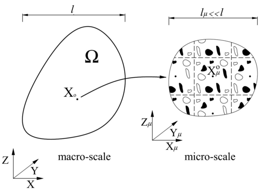
|
| Figure 24: Macrostructure and microstructure around of the point . |
The called principle of separation of scales [124] establishes that: the microstructural length scale is assumed to be much smaller than the macrostructural characteristic length , which is the length over the macroscopic space. In other words, the principle says that the existing periodical microscopic dimension around of the macrostructural point () must be smaller than the characteristic macrostructural dimension. If this principle is satisfied, the current configuration or deformed position of a material point in the RVE can be approximated as
|
|
(9.5) |
where , and is the reference configuration or non-deformed position of the material point in the RVE and and are the origin of the reference and the current coordinate system on the RVE, respectively (see Figure 25). The extra term is a microstructural displacement fluctuation field.
To simplify the symbolic manipulation of the formulation is convenient to set the coordinate system's origin as
|
|
(9.6) |
Later, it will be proved that with these values, the rigid body motion of the RVE is avoided. Considering these restrictions, the expression given by 9.5 can be rewritten as
|
|
(9.7) |
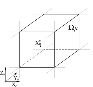
|
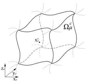
|
| Figure 25: Reference and current configuration of the RVE. | |
9.3.1 Displacement field on the RVE
The displacement field at the RVE is defined by
|
|
(9.8) |
and taking into account 9.7 in the previous equation,
|
|
(9.9) |
where is the second-order unit tensor.
9.3.2 Kinematically admissible displacement fields and boundary conditions in the RVE
The displacement fields in the RVE that are kinematically admissible are obtained as a result of the coupling between the macrostructure and the microstructure. This linkage is based on the average theorems and they have been initially proposed for infinitesimal deformations by Hill [5]. Later, Hill [125] and Nemat-Nasser [126] extended these to finite deformations.
The first of the averaging relations postulated that the volume average of the microstructural deformation gradient tensor over the RVE must be equal to the macroscopic deformation gradient tensor . In the considered point this is
|
|
(9.10) |
where is the volume of the RVE in the reference configuration.
Considering 9.7 it is possible to obtain the deformation gradient tensor in the microstructural scale as
|
|
(9.11) |
and using this relation, the right hand size of 9.10 is
|
|
(9.12) |
Equation 9.12 can be rewritten as
|
|
(9.13) |
or
|
|
(9.14) |
Finally, applying the divergence theorem, in the right hand size of 9.14, this can be also rewritten in term of surface integral as
|
|
(9.15) |
where is the RVE boundary domain in the reference configuration, and denotes the outward unit normal on .
Clearly, to satisfy the first average theorem, the integrals that depend of the displacement fluctuation in both 9.14 and 9.15 must vanish. Therefore,
|
|
(9.16) |
and
|
|
(9.17) |
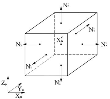
|
| Figure 26: Normal vectors to the surfaces in the reference configuration of a Cubic RVE. |
Noting Figure 25 and considering that the reference geometry configuration of the RVE is originally a cube, as the figure is showing, the integral restriction on the RVE boundary can be splitted in the different surfaces of the domain. Besides, taking the reference coordinate system that is shown in Figure 26, the outward unit normal of the cubic faces satisfy: , and . Here, the subscript makes reference to the axis which is perpendicular to the considered face and the superscript defines the position of the face on the axis. Therefore, considering this geometry, the expression given by 9.17 may be rewritten as
|
|
(9.18) |
Equation 9.18 shows that the boundary restriction on the displacement fluctuation field can be splitted on the different surface pairs (X, Y and Z) of the RVE boundary.
Previous equations from 9.16 to 9.18 can be used to obtain the different displacement fluctuation fields kinematically admissible in the microstructural level. Several models have been defined that assume different fluctuation fields, they are mentioned in the following.
(i) Taylor model (or zero fluctuations): The expression given by 9.16 is verified when
|
|
(9.19) |
This model gives homogeneous deformation in the microstructural scale level (see 9.24).
(ii) Linear boundary displacements (or zero boundary fluctuations): The expression given by 9.17 is verified when
|
|
(9.20) |
The deformation of the RVE boundary domain for this class are fully prescribed.
(iii) Periodic boundary fluctuations:
The key kinematical constraint for this class is that the displacement fluctuation must be periodic on the different faces of the RVE. That is, for each pair of boundary points the expression given by 9.18 is verified when
|
|
(9.21) |
(iv) Minimal constraint (or uniform boundary traction):
In this constraint the nontrivial solution of 9.17 is obtained.
9.3.3 Microscopic and macroscopic strain tensor
Considering a infinitesimal deformation framework the strain tensor in the microstructural level can be obtained as
|
|
(9.22) |
and, if 9.10 is satisfied it can be proved that taking the volume average of the microscopic strain tensor over the RVE domain the following relationship is obtained,
|
|
(9.23) |
Here, is the macroscopic strain tensor. Therefore, it is possible to rewrite 9.22 as
|
|
(9.24) |
where is the contribution of the displacement fluctuation field to the microscopic strain tensor and is the symmetric gradient operator. Because 9.10 is verified the volume average of over the RVE domain is equal zero.
9.3.4 Hill-Mandel principle and RVE equilibrium
The Hill-Mandel energy condition [82,127], also referred to as the macro-homogeneity condition, states that the virtual work of the point considered must be equal to the volume average of the virtual work in the RVE to any kinematically admissible displacement field, this principle can be formulated as
|
|
(9.25) |
where and are the macroscopic and microscopic stress tensor, respectively.
Using 9.24, the principle is rewritten as
|
|
(9.26) |
Taking the macroscopic stress tensor as the volume average of the microstructural stress tensor in the RVE domain, which is similar to the first average relation (see 9.10)
|
|
(9.27) |
equation 9.26 will be satisfied if
|
|
(9.28) |
Therefore, the RVE's variational equilibrium equation is
|
|
(9.29) |
which must be satisfied for any kinematically admissible displacement fluctuation field (see Section 9.3.2).
It is possible to observe that because of the symmetry of the stress tensor it can be proved that , where is a first order tensor, the 9.28 also can be rewritten as
|
|
(9.30) |
9.3.5 Microscopic and macroscopic stress tensor
The homogenized stress tensor in the macroscopic level is given by 9.27. The microscopic stress tensor can be obtained as
|
|
(9.31) |
where is the material constitutive tensor in the RVE. Then, the macro stress tensor is
|
|
(9.32) |
where,
|
|
(9.33) |
is a constitutive tensor which can be considered a microstructural material property.
Equation 9.32 shows that the stress tensor depends of the macroscopic strain tensor and also, of the microscopic strain tensor , which is obtained with the displacement fluctuation field of the RVE. Moreover, the microscopic position vector does not appear explicitly in the microstructural strain tensor expression (see 9.24). Consequently, this variable does not appear in the microstructural stress tensor either. Therefore, the periodic microstructure around the macro point does not have to be modeled with its exact dimensions. A non dimensional RVE with the internal distribution and volume fractions of the simple materials is enough to obtain the microscopic strain and stress fields. This is one of the principal advantages of this first-order homogenization approach compared to other multiscale high-order approaches.
On the other hand, it can be observed that the kinematically admissible displacement fluctuation option used to satisfy the boundary condition in the RVE problem affects the final macroscopic stress tensor obtained, as occurs in the Taylor model case. This means that if there is a null displacement fluctuation field in the total RVE domain, the stress tensor obtained only depend of the strain tensor and the constitutive tensor . In other words, the Taylor model condition returns the classical mixing theory results.
9.4 Enhanced-first-order homogenization approach
A new enhanced first order homogenization is proposed in the following, in order to enrich the displacement field of the micro model with second order information available in the macro model. The deformed position of a material point in the RVE given by 9.5, used in the first-order approach, can be improved if the second-order term of 9.3 is included. Then, it is possible to propose a new approximation of the current configuration of the RVE as
|
|
(9.34) |
and setting the coordinate system's origin as defined in 9.6, the proposed deformed position of the RVE is
|
|
(9.35) |
Therefore, the proposed displacement field on the RVE (see 9.8) can be obtained now as
|
|
(9.36) |
Noting that an extra term appears in the proposed microscopic displacement field by including the gradient of the deformation gradient tensor in 9.34. This extra second-order term is a new linking term between the macroscopic and microscopic scales. The proposed displacement field in the RVE is enhanced because it reaches more information from the macro scale.
9.4.1 Kinematically admissible displacement fields and boundary conditions in the RVE
The first of the average postulates (see 9.10) is used again to obtain the admissible displacement fields. The microscopic deformation gradient considering the expression given by 9.35 is
|
|
(9.37) |
And, the volume average of this deformation gradient over the RVE is
|
|
(9.38) |
It can be proved that if the RVE geometry in the reference configuration is originally a cube, as shown in Figure 25, and the position of the origin of the coordinate system is defined at the center of the RVE, then the first moment of volume of the RVE is
|
|
(9.39) |
Therefore, 9.38 can be rewritten as
|
|
(9.40) |
or
|
|
(9.41) |
Equation (9.41) can be rewritten in terms of surface integrals applying the divergence theorem as
|
|
(9.42) |
Equation 9.42 is exactly the same than the one obtained for the first-order approach (see 9.15) then, the restrictions on the displacement fluctuation field are the same as those shown in 9.16-9.18, and the different displacement fluctuation fields kinematically admissible presented in Section 9.3.2 are still valid for this enhanced-first-order approach.
9.4.1.1 Extra kinematic restrictions and boundary conditions because of G
The next step consists in obtaining the kinematic restrictions result of including the new term in the microscopic displacement field . In other words, some extension of the first average theorem needs to be proposed in term of the gradient of the deformation gradient. In the following, a natural extension for the first average theorem is presented. The main drawback of this proposal is that arrives to restrictions on the derivative displacement fluctuation field and therefore, a high-order problem on the RVE must be considered. To avoid this situation, and continue using the classical first-order boundary value problem on the RVE, the alternative extension proposed by Kouznetsova [115] is also presented.
Natural extension of the first average theorem
The first natural possibility for this extension could be
|
|
(9.43) |
Note that 9.43 is similar to 9.10 but in this case, the volume average of the microstructural gradient of the deformation gradient tensor over the RVE must be equal to the macroscopic gradient of the deformation gradient in the considered point .
Considering 9.37 and 9.4 the gradient of the deformation gradient in the microstructural scale is
|
|
(9.44) |
Using 9.44 and taking the volume average over the RVE it is possible to obtain
|
|
(9.45) |
or
|
|
(9.46) |
And, applying the divergence theorem in the last expression
|
|
(9.47) |
Similarly as in the first-order approach, to satisfy the proposed extension of the first average theorem, the integrals that depend of the displacement fluctuation in 9.45 and 9.47 must vanish, then
|
|
(9.48) |
and
|
|
(9.49) |
The last expression represents a new extra integral restriction on the derivative displacement fluctuation field. Taking the same consideration than before regarding the geometry of the RVE (see Figure 26), the boundary integration in 9.49 can be splitted in
|
|
(9.50) |
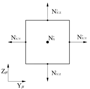
|
| Figure 27: Normal vectors to the lines in the YZ surface of the Cubic RVE. |
Some components of the integrals can also be rewritten in terms of line-boundary integrals applying the divergence theorem. For example, if the first left integral in the first term in 9.50 is taken, the line-boundary of this surface integral can be separated in four different lines, two perpendiculars to Y axis, and the other two perpendiculars to Z axis, as it is shown in Figure 27. Because of the RVE geometry considered, these lines boundary have the property of and . Then, with this information the considered integral can be rewritten as
|
|
(9.51) |
where represents the derivative with respect to the X axis, this term cannot be reduced to a line-integral using the divergence theorem. It can be seen that when the Periodic boundary fluctuations condition is the kinematically admissible option used for the displacement fluctuation field on the RVE, the two right terms on 9.51 are satisfied directly. The points on the opposing lines are a pair boundary points that have the same displacement fluctuation because of the kinematic condition imposed. Applying this same procedure to the rest of the terms of expression 9.50, this equation can be rewritten as
|
|
(9.52) |
The previous expression represents an extra restriction on the displacement fluctuation field that makes it kinematically admissible in the RVE. A possible set of boundary conditions that satisfies this restriction is
|
|
(9.53) |
Equation 9.52 is analogous to 9.18 but it is written in terms of derived displacement fluctuation field, in this case, on the normal direction of the pair surfaces (see Figure 26). Therefore, to satisfy any kinematic restriction, as for example 9.53, obtained from 9.52 a high-order problem on the microscopic scale must be considered because the restriction of the displacement fluctuation field is written on its derivate.
Alternative extension of the first average theorem
An alternative to the proposed extension of the averaging theorem given by 9.43 should be found to keep a classical boundary value problem on the microstructural RVE problem. With this aim Kouznetsova [115] proposed another alternative extension of the first average theorem. The proposed condition imposes that the second moment of area of the deformed RVE, given in terms of the microscopic displacements, must be equal to the second moment of area of the RVE expressed in terms of macroscopic deformation variables [121]. Considering the above, the expression given by 9.37 is multiplied by and integrated over the RVE volume to obtain
|
|
(9.54) |
Knowing that the first moment of volume of the undeformed RVE is zero (see 9.39), and defining the second moment of volume of the undeformed RVE as . Equation 9.54 can be rewritten as
|
|
(9.55) |
replacing the following relationships
|
|
(9.56) |
and
|
|
(9.57) |
it is obtained
|
|
(9.58) |
Using 9.35 it can be shown that
|
|
(9.59) |
which is used to obtain the final version of the sought expression
|
|
(9.60) |
Applying the divergence theorem on the right hand size of the equation, it can be rewritten in term of surface integral as
|
|
(9.61) |
It is possible to make a parallelism between 9.15 and 9.61. The additional condition regarding the second moment of area of the deformed RVE given by 9.54 requires that the influence of the displacement fluctuation field should vanish, then
|
|
(9.62) |
Equation 9.62 is a boundary restriction for the displacement fluctuation field, then it is not necessary a high-order boundary value problem, at microscopic scale, to satisfy the new boundary conditions deduced from it. Considering again the cubic geometry in the reference configuration defined previously for the RVE (see Figure 26), the restriction given by 9.62 can be splitted in the different surfaces of the domain as
|
|
(9.63) |
The last expression is used in Section 9.5.2 to obtain the boundary value problem on the RVE for the enhanced-first-order approach. In the case of Periodic boundary fluctuations condition, it can be proved that the expression 9.63 is automatically satisfied if
|
|
(9.64) |
Therefore, the extra boundary condition required in this case is that the integral of the periodic displacement fluctuations on the RVE surfaces must be zero.
9.4.2 Microscopic and macroscopic strain tensor
In this enhanced-first-order homogenization approach, the strain tensor of the microstructure for an infinitesimal deformation approach can be written as
|
|
(9.65) |
Knowing that 9.10 is satisfied and using equation 9.39, the resulting expression of the volume average of the microscopic strain tensor over the RVE domain is the same than 9.23, which was obtained previously in Section 9.3.3. Therefore, the microscopic strain tensor can be rewritten as
|
|
(9.66) |
where is a new term in the microscopic strain tensor, resulting from including the second-order term in the formulation. Using the expression given by 9.39, it can be proved that the volume average of this new term over the RVE domain is equal to zero.
9.4.3 Hill-Mandel principle and RVE equilibrium
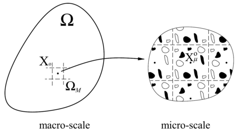
|
| Figure 28: Macro volume around point and its micro structure. |
When the second-order of the Taylor series expansion given by 9.3 is used to improve the approximation of the deformed position of a material point in the RVE (see 9.34), it is assumed that exists a macroscopic finite volume around the considered point , as it is shown in Figure 28. This finite volume must be smaller than the characteristic macroscopic dimension. Therefore, the Hill-Mandel principle should be applied now not only taking into account the virtual work of the point , but considering the volume average of the virtual work in the macro volume . This can be stated as
|
|
(9.67) |
The macroscopic deformed position of a material point in around the point can be approximated with a second-order approach using 9.3 as
|
|
(9.68) |
and the approximated macroscopic deformation gradient is
|
|
(9.69) |
The macroscopic strain tensor in the domain for infinitesimal deformation approach can be then approximated as
|
|
(9.70) |
or
|
|
(9.71) |
where .
Taking into account 9.66 and 9.71, the expression given by 9.67 can be rewritten as
|
|
(9.72) |
and because of the symmetry of the stress tensor, it can be proved that and , where is a first order tensor. Then, 9.72 is finally
|
|
(9.73) |
Following the same procedure used in Section 9.3.4 to satisfy the Hill-Mandel principle, it is necessary to define the following tensors:
|
|
(9.74) |
where is the homogenized stress tenor, which is obtained as the volume average of the stress tensor around the point , and
|
|
(9.75) |
where is the homogenized second-order stress tensor in the point , which is a the three-order tensor. Finally, the RVE's variational equilibrium equation is
|
|
(9.76) |
that must be satisfied for any kinematically admissible displacement fluctuation field shown in Section 9.4.1.
9.4.4 Homogenized stress and second-order stress tensor
The microscopic stress tensor can be obtained as
|
|
(9.77) |
then, the homogenized stress tensor at the macroscopic scale given by 9.74 is
|
|
(9.78) |
or
|
|
(9.79) |
where
|
|
(9.80) |
The tensor can be also considered a microscopic material property. This constitutive tensor relates gradient of the deformation gradient tensor , to the homogenized stress tensor , and generates a coupling effect. This tensor is analogous to the called bending-extension coupling matrix used in plates or shells theories [12].
Equation 9.79 shows that the homogenized stress tensor in the point depends of the macroscopic tensor and , of the microscopic displacement fluctuation field and also, of the vector position of the RVE. Considering now a particular case where the simple materials within the RVE are symmetrically located respect to the coordinate system's origin, which has been placed on the RVE geometric center (see Section 9.4.1). It can be proved that taking this symmetric distribution of the simple materials the value obtains for the constitutive tensor is zero. Therefore, the homogenized stress tensor for this case can be rewritten as
|
|
(9.81) |
The macroscopic second-order term and of the vector position do not affect the homogenized stress tensor. The expression given by 9.81 is the same than the one obtained for first-order homogenization given by 9.32.
On the other hand, the homogenized second-order stress tensor can be obtained using 9.75 and the microscopic stress tensor given by 9.77 as
|
|
(9.82) |
or
|
|
(9.83) |
where
|
|
(9.84) |
The tensor is also considered a microscopic material property, which is obtained with the RVE model, as it is done with tensors and . Taking into account the symmetric distribution materials inside the RVE, the expression for the homogenized second-order stress can be written as
|
|
(9.85) |
Equation 9.85 shows that the second-order stress tensor depends on the macroscopic tensor and on the microscopic displacement fluctuation field . But it also depends on the vector position of the material point in the RVE. In addition, the tensor does not vanish because of the symmetric materials distribution.
9.4.5 Final remarks on the enhanced-first-order homogenization approach
In the enhanced-first-order approach is lost the benefit shown by the first-order approach regarding the possibility of using a non dimensional RVE. The microscopic strain 9.66 and stress 9.77 tensor now have an explicit dependence with the material vector position in the RVE. This dependence has been observed also in the homogenized second-order stress tensor 9.85. While the homogenized stress tensor 9.81 is not dependent of when a symmetric internal distribution of the materials is taken. Besides, to satisfy 9.72, which is obtained from the Hill-Mandel condition extended to the enhanced-first-order approach, it is necessary to impose that . Thus the RVE's dimension used to characterize the microstructure should be equal than the size of the finite volume around the considered point . Then, the enhanced-first-order homogenization procedure can be understand as a domain decomposition where the sub-domains have a periodic microstructure.
However, the enhanced-first-order homogenization is better than the first-order homogenization from a microscopic point of view. Although the homogenized stress tensor for both theories is the same, the microscopic displacement field, the microscopic strain and, the stress tensors are not equal. The enhanced-first-order approach gets a better approximation of the microscopic behavior because it accounts for the information provided by the macroscopic second-order term . Therefore, in a non-linear analysis, the initiation and the evolution of the non-linear performance of the microstructure will be better characterized if the enhanced-first-order formulation is used.
On the other hand, a detailed analysis of the formulation shows that the first-order homogenization theory is contained in the enhanced-first-order one. Therefore, when the principle of separation of scales is verified, the results obtained using the enhanced formulation will be the same than the ones obtained using the first-order homogenization. In other words, if the periodic microstructural length scale is much smaller than the structure characteristic length (see Figure 24), the contribution of the extra term considered in 9.35 to improve the first-order approach is negligible.
The variational equilibrium equation obtained in the microstructure for both homogenization formulations is the same 9.29 and 9.76. However, in the enhanced-first-order homogenization formulation extra boundary conditions must be satisfied. High-order boundary conditions 9.53 are obtained if the natural extension of the first average theorem is proposed 9.43. In consequence, this kind of extra boundary conditions require a high-order microscopic equilibrium equation. To avoid this situation an alternative extension of the average theorem given by 9.60 is used to conserve a first-order microscopic variational problem. New extra boundary conditions using 9.60 for the case of Periodic boundary fluctuations are obtained and shown in the expression 9.64. Finally, for the enhanced-first-order approach, a macroscopic second-order stress tensor is obtained from the RVE solution. This high-order stress tensor should be considered in the macroscopic scale theory.
9.5 Macroscopic and microscopic formulation
In the following, the boundary value problem (BVP) in the macroscopic and in the microscopic scales are presented.
9.5.1 Macroscopic BVP
A BVP is considered for the macrostructural scale of a domain with a periodic internal microstructure. The kinematics of the problem is related to a displacement field on the macroscopic scale, which provides the displacement of each material point of the domain . From a continuum mechanics approach the macroscopic BVP is
|
|
(9.86) |
where is the macroscopic stress tensor, and is the internal body force associated to the mass forces of the material. The boundary of () is defined disjointedly by the surfaces where the macroscopic displacement is known (Dirichlet's condition) and where the macroscopic surface load are known (Neumann's condition) with and . Finally, are the components of an outward vector normal to the surface .
The resolution of the BVP given by 9.86 consists on the determination of the macroscopic displacement field corresponding to the solution , where is the set of continuous and sufficiently regular functions with zero-valued in . The partial differential equation in the macroscopic BVP above presented can be rewritten in a weak form (or variational form) as
|
|
(9.87) |
where are the called test functions. Equation 9.87 can be rewritten, applying the divergence theorem, as
|
|
(9.88) |
Considering infinitesimal deformations, the macroscopic strain and stress tensor are
|
|
(9.89) |
9.5.2 Microscopic BVP
The obtained variational equilibrium statement (or the virtual work equation) in the microstructure (see 9.29 and 9.76) can be written as
|
|
(9.90) |
Considering again an infinitesimal deformation, the microscopic strain tensor is
|
|
(9.91) |
where is the symmetric gradient of the microscopic displacement field in the RVE and is the set of continuous and sufficiently regular kinematically admissible RVE displacement fields. Further, it is assumed that in the microstructure the constitutive behavior is described by conventional internal dissipative constitutive theories. Therefore, the microscopic stress tensor is obtained by integrating the constitutive equations, knowing a set of internal variables , for the given strain tensor history. Then, it is
|
|
(9.92) |
With the above at hand, the resolution of the microstructure problem consists on the determination of the microscopic displacement field of the variational problem for a given macroscopic deformation gradient tensor , and its gradient in enhanced-first-order approach case. Therefore, to complete the BVP in the microscopic scale it is necessary to define the boundary condition used to obtain kinematically admissible displacement fields from the solution of 9.90.
9.5.2.1 First-order approach
In Section 9.3.2, the different displacement fluctuation fields, kinematically admissible in an homogenization analysis, were obtained. Using 9.9 is possible to obtain the boundary condition for each case in terms of the displacement field as
(i) Taylor model (or zero fluctuations):
|
|
In this model is not necessary to solve the BVP defined by 9.90.
(ii) Linear boundary displacements (or zero boundary fluctuations):
|
|
In this case a classical BVP with only Dirichlet conditions is obtained.
(iii) Periodic boundary fluctuations:
|
|
In this case, the boundary condition is a constraint boundary condition.
(iv) Minimal constraint (or uniform boundary traction):
|
|
For this case, the boundary condition is an integral constraint boundary condition.
9.5.2.2 Enhanced-first-order approach
In Section 9.4.1, the different displacement fluctuation fields kinematically admissible were obtained for the enhanced-first-order approach. Besides, with this approach exists an extra restriction on the displacement fluctuation field because the term is introduced in the microscopic displacement field. Using 9.36 it is possible to obtain the boundary condition for each case in terms of the displacement field as
(i) Taylor model (or zero fluctuations):
|
|
In this model is not necessary to solve the BVP defined by 9.90.
(ii) Linear boundary displacements (or zero boundary fluctuations):
|
|
A classical BVP with only Dirichlet conditions is obtained because the extra boundary restriction 9.62 is automatically verified.
(iii) Periodic boundary fluctuations:
|
|
To satisfy the extra boundary restriction given by 9.64 extra boundary conditions are required. These are:
|
|
In this case, one boundary condition is a constraint boundary condition and the extra boundary condition is an integral constraint boundary condition.
9.5.3 Consequence of the boundary condition considered
The RVE has a finite dimension, which is opposed to the theoretically infinite microstructure considered, which create the intrinsic problem of the non-physical RVE edges. As a result, the election of the boundary condition in the RVE problem is essential to characterize the real behavior of the microstructure. The boundary conditions shown in the above sections are obtained from the restriction on the microscopic displacement fields by the first average postulate 9.10 and they are used to impose the driving macroscopic deformation gradient tensor (or strain tensor) on the RVE. Besides, these boundary restrictions should incorporate the presence of the surrounding material of the RVE without (or minimizing) the introduction of spurious effects.
9.5.3.1 Effects on the characterization of the material properties
It has been shown in Section 9.3.5 that the boundary condition used in the RVE problem affects the macroscopic stress tensor obtained and therefore it also affects the homogenized constitutive tensor. In example, the expression 9.32 shows that using the Taylor model condition, which in fact is not a strictly boundary condition, the result provides an upper bound of the estimated homogenized microscopic stiffness, which is exactly the same that is predicted by the classical mixing theory.
On the other hand, the Minimal constraint provides a lower bound of the estimated effective microstructural stiffness. This boundary condition imposes the macroscopic strain tensor on the RVE in the weakest sense. It has been shown that the resulting boundary distribution of the microscopic stress tensor in the RVE is uniform and equal to the macroscopic stress tensor in this boundary restriction [118,128].
The Linear boundary displacements condition is a too restrictive constraint and it overestimates the homogenized microscopic stiffness [129]. A conventional BVP with full Dirichlet's condition is obtained for the microstructure when this condition is addressed.
It has been shown in the literature that in general the Periodic boundary fluctuations provide a better apparent stiffness estimate for both periodic as well as random microstructures [101,130,118,131,132,133,134]. This condition makes that the RVE self adjoint by point to point (pairs of points) coupling of boundary displacements, thereby it naturally incorporates the mechanical response of the surrounding material. Moreover, an anti-periodic condition of the boundary forces is automatically fulfilled in the microscopic problem because the boundary points of the RVE are really considered as internal points of the structure.
9.5.3.2 Effects on the non-linear response
Besides obtaining effective properties of the material at the macrocopic scale, RVE models have been also used to study damage and strain localization effects [135,136,137,138,139]. There is a significant interaction between both phenomena, when the damage occur within the RVE, small zones with high strains coalesce to form a strain localization band. If the macroscopic loading increases continuously, the microscopic strain localizes on this band, accelerating the damage development and reducing the load capacity and finally resulting in strain softening in the macroscopic scale.
The boundary conditions imposed in the microscopic BVP need to address the beginning and the development of the localization band up to the point of macroscopic localization. Too restrictive boundary constraints, such as the Linear boundary displacements case will suppress the development of the microscopic localization band, and searching an alternative localization pattern, it will overestimate the predicted macroscopic strain softening load.
The Periodic boundary fluctuations condition allows the onset of a localization path compatible with the periodicity constraints, such as horizontal, vertical, multiple parallel inclined bands and etc [138].
In order to do not restrict the development of the localization band within the RVE the Minimal constraint conditions have been used as an alternative to the others showing that the localization paths can cross the RVE in arbitrary manner [140,141]. However, besides the underestimation of the effective microstructural stiffness, this boundary condition is also sensitive to spurious localization in weak zones near the RVE boundary, resulting in an unrealistically early onset of macroscopic failure [129].
Base on the different performance described, in this work the Periodic boundary fluctuations condition will be used in the computational implementation of the microscopic BVP for both homogenization approaches considered, first-order and enhanced-first-order.
9.6 Finite element implementation
The numerical implementation of the developed homogenization approaches is made through the FEM. This method splits the total domain of the problem in finite N-subdomains, known as Finite Element (FE) where the unknown displacement field is approximated using known displacements of some points (called nodal points) and shape functions.
When the FEM is used to solve the weak formulation of a BVP the total integration domain of the problem is separated in N-subdomains which are the FE domains. The value of the definite integral in the FE domain is obtained using some numerical integration procedure. In general, the numerical integration methods approximate the integral value as the weighted sum of the evaluated integrand in a finite set of points called integration points. These integration points, and their weights, depend on the accuracy required and on the integration method. In the following, the selected method will be the Gaussian quadrature rule which uses n-points () called Gauss points and n-weights () to obtain the numerical approximate value of the integral.
To solve the BVP at the macroscopic scale for linear and non-linear range a FEM implementation is used together with a Newton-Raphson iterative scheme. Therefore, it will be necessary to know the macroscopic stress tensor on the integration points of the FEs in the macro domain. To achieve the stress tensor in the FE domain it is required a constitutive model to describe the composite behavior. The multiscale homogenization approaches above described can be chosen as the constitutive models. Consequently, the macroscopic stress tensor is obtained through the analysis of the microscopic scale. The macroscopic deformation gradient tensor (), for the first-order homogenization, and its gradient tensor (), for the enhanced-first-order homogenization, are used to solve the microscopic BVP. The microscopic solution is used to obtain the homogenized stress tensor required to solve the macroscopic BVP through the FEM.
The macrostructural point considered in the formulation represents physically the Gauss points on the FE. Therefore, the macroscopic values of the deformation gradient tensor and the gradient of the deformation gradient tensor , required by the microscopic BVP, are obtained in these Gauss points when the macroscopic BVP is solved.
9.6.1 Microscopic numerical implementation
As has been done at the macroscopic scale, the BVP at the microscopic scale is solved using the FEM. Therefore, the unknown displacement field in the BVP is reduced to a finite degrees of freedom, which are the nodal displacements at the nodal points of the FEs. At this scale the microscopic displacement field obtained from the solution of the RVE must satisfy the boundary conditions defined previously, in Section 9.5.2.
If the Taylor model condition is considered, there is no BVP to solve because the displacement field on the total microscopic domain is constrained by the condition. For the case of Linear boundary displacements condition, a conventional BVP is obtained with a Dirichlet's condition on the whole boundary domain. Finally, the cases of Periodic boundary fluctuations and Minimal constraint conditions defined a BVP with constraint boundary conditions.
The restrictions of degrees of freedom on the boundary domain can be accounted through several methods such as elimination of redundant unknowns, penalty methods and Lagrange multipliers [105]. The last two methods have the disadvantage that they lead to ill-conditioned stiffness matrix or to an increase of the number of degrees of freedom of the problem.
To avoid these two disadvantages, here it is proposed solving the RVE by an elimination of redundant unknowns [142]. The constraint condition for the Periodic boundary fluctuations is shown in Section 9.5.2, where it is possible to observe the redundant boundary unknowns of the BVP. In these boundary constraint expressions it is possible identify master unknowns (the unknowns to solve) and slave unknowns. In Appendix B.1 the master-slave kinematic relationships are derived for the Periodic boundary fluctuations condition.
9.6.1.1 Linear implementation
Following a conventional notation, the FE approximation of the variational problem 9.90, for a given discretization h, consists in the determination of the unknown vector of the microscopic global nodal displacement such as
|
|
(9.93) |
where denotes the discretized domain of the RVE, is the global strain-displacement matrix (see Appendices B.3 and B.4), is the global vector of nodal displacement fluctuation, is a set of internal variables and is the set of finite-dimensional nodal displacement vectors associated with the FE discretization h of the RVE domain . If a linear case is considered, the microscopic stress tensor is
|
|
(9.94) |
therefore, 9.93 can be written as
|
|
(9.95) |
or
|
|
(9.96) |
where,
|
|
(9.97) |
Here, is the global stiffness matrix.
Equation 9.96 does not include the boundary constraint on the unknown nodal displacement field because of the Periodic boundary fluctuations condition as it was explained in the preceding section. If this conditions are applied using an elimination of redundant unknowns method, the following system of equations is obtained
|
|
(9.98) |
where, is the reduced global stiffness matrix, the reduced global nodal displacements vector and is the Right-Hand Side global vector which is obtained as a result of the applied boundary restriction. Section B.2.1 of Appendix B.2 shows how the elimination of redundant unknowns is addressed to obtain the expression given by 9.98.
9.6.1.2 Non-linear implementation
The solution of the FE approximation of the microscopic variational problem given by 9.90 in the non-linear case is addressed by a Newton-Raphson iterative scheme. Therefore, the microscopic displacement field for a typical iteration in the micro-scale is obtained according to the following update expression
|
|
(9.99) |
where is the unknown iterative displacement field. Considering that the microscopic stress tensor can be obtained as
|
|
(9.100) |
and taking the following approximation
|
|
(9.101) |
with
|
|
(9.102) |
denoting the microscopic tangent constitutive tensor. With the above at hand, and for the given discretization , the FE approximation of the microscopic problem consists in solving the unknown iterative of the global nodal displacement vector of the following equation
|
|
(9.103) |
or
|
|
(9.104) |
where,
|
|
(9.105) |
and
|
|
(9.106) |
is the global tangent stiffness matrix of the RVE.
Like in the linear case, 9.104 does not include the boundary constraint over the RVE boundary because of the Periodic boundary fluctuations condition. If this condition is applied using an elimination of redundant unknowns method, the expression given by 9.104 can be rewritten as (see Section B.2.2 of Appendix B.2)
|
|
(9.107) |
where, is the reduced global tangent stiffness matrix, the reduced iteration of the global nodal displacements vector and is the global RHS vector of the previous iteration.
9.7 Final remarks
Based on the characteristics of the formulations developed, as well as on the implementation of these formulations when using the finite element method, in the following are included some final remarks regarding the implications of using the first-order or the enhanced-first-order models.
Let us assume, for the sake of simplicity, that the FE mesh of the macroscopic model has a single integration point. In this case, the macroscopic finite volume around the point considered in the formulation is related with the FE domain as , where is the FE domain. Taking into account the considerations made in Section 9.4.5 it can be concluded that , which means that for the integration point of the FE, the RVE domain must be geometrically equal to the FE domain. Consequently, for an enhanced-first-order approach the RVE dimension is related with the discretization mesh used in the macroscopic BVP.
The macroscopic BVP presented in Section 9.5.1 does not take into account the homogenized second-order stress tensor obtained in the enhanced-first-order homogenization. Besides, if the RVE materials are symmetrically distributed in it, the estimated homogenized stress tensor obtained is the same with both homogenization approaches. Therefore, the homogenization method considered does not improve the macroscopic results obtained for the BVP. To improve the macroscopic results, a high-order FE or enhanced FE mesh must be considered. To account for the homogenized second-order stress tensor in the macroscopic scale a second-order macroscopic formulation must be used [115,8,116].
9.7.1 Linear FE in the macroscopic mesh
In linear finite element the interpolation functions are first-order polynomials and consequently, the displacement field in the domain of the FE is a first-order function. The strain tensor is obtained by differentiating the displacement field, and then the strain tensor in the FE will be a constant function. Therefore, a fine FE mesh on the macroscopic BVP should be used to obtain an accurate approximation of the strains and stresses.
When linear finite elements and a first-order homogenization are used to solve the macroscopic problem, the RVE is just a representative sub-domain of the periodic microstructure that does not have any significance on real microscopic dimension as has been shown in Section 9.3.5. The constant value of the macroscopic gradient tensor in the integration point of the macroscopic FE is used to define the BVP in the RVE. From the solution of the microscopic problem the macroscopic stress tensor is obtained for the considered integration point.
In this case, the solution of the microscopic BVP with the enhanced-first-order homogenization is an inefficient procedure because the value of in the integration point of the macroscopic linear element has partial or even zero information.
9.7.2 High-order FE in the macroscopic mesh
To improve the FEM approach high-order elements can be used. Quadratic finite elements use second-order polynomials as interpolation functions to approximate the displacement field within the FE's domain. The deformation gradient tensor of this element is a first-order function, while gradient of the deformation gradient tensor , which is obtained deriving twice the displacement, is a constant function on the FE domain.
The enhanced-first-order homogenization approach needs at least quadratic elements in the macroscopic mesh in order for the functions and not to have zero value in the FE domain. Quadratic elements need more than one Gauss point to obtain the best integration approximation. As mentioned before, the RVE dimension must be related with the FE dimension in this enriched first-order homogenization. For quadratic elements, the RVE must represent the sub-domain within the FE associated to the Gauss point. Because the deformation gradient is not a constant function on the Gauss point domain, the RVE should not be modeled with a different periodic sub-domain of the microstructure.
In this case, the microscopic results depend of the dimension of the RVE. Therefore, to obtain the best possible approximation of the strain and stress fields using the enhanced-first-order approach, and high-order finite elements in the macroscopic mesh, the RVE geometry should represent the real volume of the surrounding domain in the Gauss point. If not, the analysis will have an associated error due to the size mismatch.
9.8 Numerical example
The objective of this section is to show the advantages and drawbacks of the enhanced-first-order computational homogenization with respect to the first-order approach through numerical examples.
Two numerical example have been analyzed with the same macroscopic geometry, the first one uses a homogeneous material and the numerical solution obtained for both procedures are compared with the existing analytical solution. The second numerical simulation uses a matrix with a long fiber reinforcement.
9.8.1 Geometry, support scheme and mesh information
9.8.1.1 Macroscopic Beam model
The chosen macroscopic structure is a three-dimensional fixed support beam that is subjected to a fixed displacement () at the free end. Figure 29 shows the dimensions and the support scheme on the geometry of the beam.
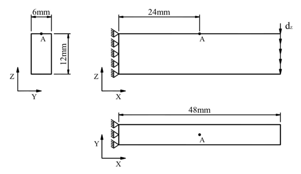
|
| Figure 29: Dimensions of the geometry and support scheme of the structure simulated. |
To study the numerical stability and convergence of the problem four mesh sizes are simulated. Linear element and quadratic element are used in the different meshes of the numerical model for the first-order homogenization case while only quadratic FEs are used for the enhanced-first-order approach. The linear FE is an hexahedron of 8 nodes and 8 Gauss points and the quadratic FE is an hexahedron with 20 nodes and 27 Gauss points.
| Mesh | Linear elements | Quadratic elements | ||||
| Elements | Nodes | Gauss | Elements | Nodes | Gauss | |
| Macro1 | 8x1x2 | 54 | 128 | 8x1x2 | 165 | 432 |
| Macro2 | 16x2x4 | 255 | 1024 | 16x2x4 | 869 | 3456 |
| Macro3 | 32x4x8 | 1485 | 8192 | 32x4x8 | 5433 | 27648 |
| Macro4 | 64x8x16 | 9945 | 65536 | 64x8x16 | 37937 | 221184 |
Table 8 shows the more relevant information about the macroscopic meshes used for the numerical simulation. These meshes are graphically show in Figure 30.
|
|
| (a) Mesh Macro1 | (b) Mesh Macro2 |
|
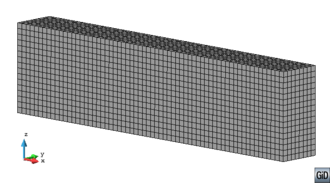
|
| (c) Mesh Macro3 | (d) Mesh Macro4 |
| Figure 30: Different mesh sizes used in the macroscopic numerical model. | |
9.8.1.2 Microscopic RVE model
The geometry design of the RVE depends of the numerical simulation case. For the case of a homogeneous material, the RVE is a simple cube with length L, this is shown in Figure 31a. In the second simulation case, the material defined is a composite with a 40% of cylindrical long fiber volume. The geometry of the RVE that represents this periodical microstructure is shown in the Figure 31b.
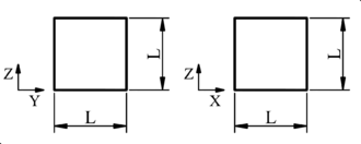
|
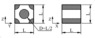
|
| (a) RVE for homogeneous material. | (b) RVE for composite material. |
| Figure 31: RVE models for the two different numerical simulation cases. | |
It has been shown in previous section that the dimension of the RVE is an important parameter for the enhanced-first-order homogenization approach. Moreover, this dimension L is directly related with the volume around the Gauss point of the FE in the macroscopic mesh. Therefore, the value of the length L depends of the dimension of the FE used in the numerical macro-model and of the number of Gauss points of the FE. In Table 9 the number of elements in the beam height, Z direction, and the value that takes the length L in the RVE for the different macroscopic meshes used are shown. The value of the length L has been calculated considering quadratic element on the macroscopic mesh.
| Data | Macro1 | Macro2 | Macro3 | Macro4 |
| Num. elem. | 2 | 4 | 8 | 16 |
| Length L [mm] | 1.3525 | 0.6762 | 0.3381 | 0.1691 |
The RVE has been analyzed with just one FE model. Figure 32a shows the mesh used in the RVE for the homogeneous material case, which has 1000 FE, and Figure 32b shows the mesh of the RVE for the composite material that has 1936 FE.
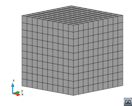
|
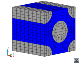
|
| (a) Mesh for homogeneous material. | (b) Mesh for composite material. |
| Figure 32: Mesh used on the RVE models for the different numerical simulations. | |
9.8.2 Results and analysis
9.8.2.1 Checkpoints and variables compared in the simulation
The reaction force in Z direction on the fixed support is a variable used for the comparison. To compare not only this macroscopic variable another checkpoint has been designed. The macroscopic stress value is compared in the macroscopic Gauss point closest to point A and the microscopic stress obtained in the RVE is also compared for this same Gauss point. The microscopic stress value used for the comparison is the one obtained in the Gauss point closest to point A within the RVE. The geometric point A is shown in Figure 29 of the beam simulated. The longitudinal stress values () and the shear stress values () will be compared on this point.
9.8.2.2 Homogeneous material simulation
When the material used in the beam is a homogeneous material it is possible to obtain the analytical solution for the support scheme shown in the Figure 29. The reaction force in Z direction is given by
|
|
(9.108) |
where and is the Young's modulus and shear modulus of the material, respectively, while , and is the second moment of area, the cross section area and the longitudinal length of the beam, respectively. Therefore, considering an isotropic material with null Poisson's ratio and taking a fixed displacement of mm, it is possible to address the values shown in Table 10 from the analytical solution. The and values shown in table correspond to the analytical values obtained in point A.
| Data | [MPa] | [MPa] | [N] | [MPa] | [MPa] |
| Values | 26560 | 13280 | 600 | 100 | 0 |
The numerical results obtained for the different approaches and meshes are presented in a simplified form using tables and graphs. On the tables, the relative error or absolute error obtained when comparing the result with the analytical solution is also shown.
Table 11 shows the reaction force in Z direction obtained with the numerical simulations. In this table, the results obtained with Linear Elements (LE) in the macro-model and the First-Order (FO) homogenization approach are shown in the first two columns. The following two columns show the results obtained with Quadratic Elements (QE) and the FO approach. And, in the last two columns, are included the results obtained with QE for the macro model, and the Enhanced-First-Order (EFO) approach.
| [N] | LE&FO | % | QE&FO | % | QE&EFO | % |
| Macro1 | 679.09 | 13.18 | 600.43 | 0.07 | 600.43 | 0.07 |
| Macro2 | 620.03 | 3.34 | 600.12 | 0.02 | 600.12 | 0.02 |
| Macro3 | 605.09 | 0.85 | 600.09 | 0.01 | 600.09 | 0.01 |
| Macro4 | 601.34 | 0.22 | 600.08 | 0.01 | 600.08 | 0.01 |
It is possible to observe that the results do not change when a Enhanced-first-order approach is used. This is because the EFO do not improve the macroscopic solution, the macroscopic stress field obtained is the same than the one obtained with a FO approach, and therefore the reaction forces are also the same (see Table 12). Another interesting conclusion obtained from the results is that an increase in the order of the macro FE model represents a meaningful improvement. The mesh Macro1 with QE obtains best results than the mesh Macro4 with LE, which is surprising because Macho4 has 16 FE in the beam height. Figure 33 shows the curves of reaction force vs number of finite elements in the beam height. This curve shows clearly the result previously addressed.
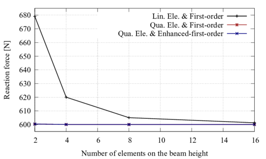
|
| Figure 33: Reaction force vs number of elements in Z direction for the different approaches. |
Table 12 shows the macroscopic longitudinal stress obtained from the numerical simulations and the relative error of these numerical results using the analytical result [MPa] as reference. The stress values shown in the table correspond to the ones obtained for the Gauss point closest to point A on the beam meshes. It has to be noted that for large meshes, the relative error is slightly increased by the distance between the Gauss point and the point A considered.
| [MPa] | LE&FO | % | QE&FO | % | QE&EFO | % |
| Macro1 | 69.43 | 30.57 | 86.08 | 13.92 | 86.08 | 13.92 |
| Macro2 | 84.02 | 15.98 | 93.00 | 7.00 | 93.00 | 7.00 |
| Macro3 | 91.82 | 8.18 | 96.50 | 3.50 | 96.50 | 3.50 |
| Macro4 | 95.86 | 4.14 | 98.25 | 1.75 | 98.25 | 1.75 |
The improvements of the EFO approach can be seen when comparing the microstructure results provided by the RVEs used in the macroscopic Gauss point closest to point A. The longitudinal stress and shear stress present in the following tables and figures are the microstructure stress values of the Gauss point in the RVE closest to point A. Table 13 shows the value of the longitudinal stress obtained within the RVE for the Gauss point closest to point A. This table shows that the results provided by the EFO model are always closer to the analytical ones, as the model is capable of capturing the bending effects on the material.
| [MPa] | LE&FO | % | QE&FO | % | QE&EFO | % |
| Macro1 | 69.43 | 30.57 | 86.08 | 13.92 | 98.66 | 1.34 |
| Macro2 | 84.02 | 15.98 | 93.00 | 7.00 | 99.59 | 0.41 |
| Macro3 | 91.82 | 8.18 | 96.50 | 3.50 | 99.87 | 0.14 |
| Macro4 | 95.86 | 4.14 | 98.25 | 1.75 | 99.96 | 0.04 |
Figure 34a shows the stress obtained as a function of the number of elements in the beam height. The general behavior of the stress when the number of elements increase is similar. When a EFO approach is used the estimation of the stress is good even for large elements. The relative error for 2 elements case is around 1% which represents a very good estimation.
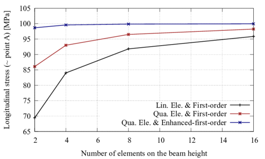
|
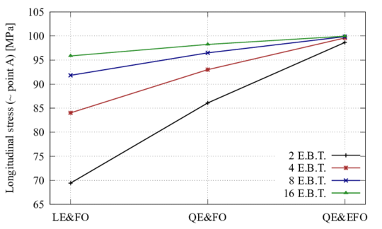
|
| (a) vs number of elements on the beam height. | (b) vs approach used in the simulation. |
| Figure 34: Longitudinal stress obtained close to point A for the different meshes and approaches used. | |
Figure 34b shows the longitudinal stress as a function of the approach used in the numerical simulation. The improvement of the stress obtained when the approach changes can be approximated as a linear function. If the number of elements in the height increase the slope of the function decreases. Therefore, the benefit of change the approach is more significant for meshes with low number of elements.
| ||||||||||||
| Figure 35: Macroscopic and Microscopic (RVE closest to point A) field for the mesh Macro3. |
As an example of the macroscopic and microscopic longitudinal stress field obtained for the different approaches the Figure 35 shows for the mesh case Macro3. For the FO approach this figure shows an uniform stress distribution in the RVE, this is because the formulation only uses the macroscopic deformation gradient to solve the RVE. This occurs independently of the macro elements uses, LE or QE. The macroscopic improvement observed in the QE model is because the solution of the macroscopic problem is better when this kind of element is used. For the same macroscopic solution, if an EFO approach is used, the approximation of the microscopic stress field improves. The RVE stress field shows a not uniform distribution (see QE&EFO case) because the EFO formulation can considered second-order effects in the microstructure.
The results obtained for the shear stress in the RVE for the Gauss point closest to point A are shown in Table 14. This table also shows the absolute error, here it is not used the relative error because for this variable the analytical value obtained in the geometric point A is [MPa]. Figure 36a shows the shear stress obtained for the different approaches as a function of the number of elements in the height of the beam. From the table and the figure it is possible to observe that the main improvement in the shear stress results it is presented when the FE is changed. This phenomenon can be observed more clearly in Figure 36b which shows the shear stress as a function of the approach used. However, the use of the EFO approach improves the shear stress obtained for all meshes considered. The reason for this improvements is, as has been pointed out with the value, the capacity that the EFO formulation gives to the RVE model to account for the second-order effects existing in the macro model.
| [MPa] | LE&FO | QE&FO | QE&EFO | |||
| Macro1 | -22.14 | 22.14 | -3.90 | 3.90 | -1.88 | 1.88 |
| Macro2 | -12.26 | 12.26 | -1.68 | 1.68 | -0.48 | 0.48 |
| Macro3 | -6.43 | 6.43 | -0.77 | 0.77 | -0.13 | 0.13 |
| Macro4 | -3.29 | 3.29 | -0.37 | 0.37 | -0.04 | 0.04 |
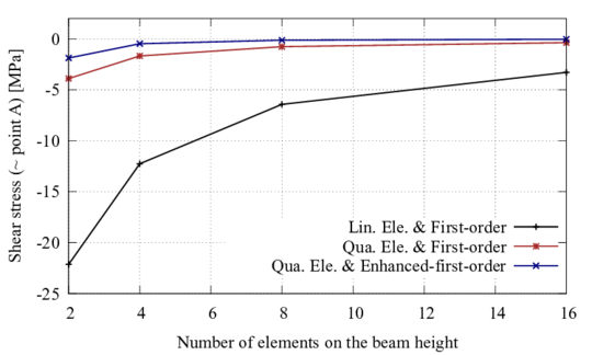
|
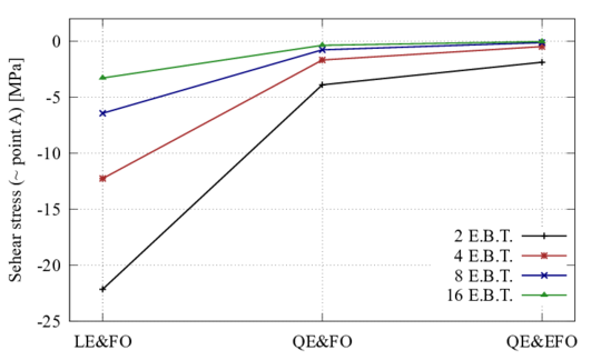
|
| (a) vs number of elements on the beam height. | (b) vs approach used in the simulation. |
| Figure 36: Shear stress obtained close to point A for the different meshes and approaches used. | |
9.8.2.3 Composite material
In the following numerical simulations, the material used is a composite with long fibers. The RVE used to simulate the internal structure of this composite is shown in Figure 31b, while the FE mesh used is shown in Figure 32b. The material used for the matrix is an elastic isotropic material (resin epoxy HSC Epikote 4652) with a Young's modulus of [GPa] and a Poisson's ratio of . The long fiber material considered is a carbon fiber (Grafil TR30S 3K carbon fiber) with a [GPa] and . The materials properties have been taken from the work of Perez et al. [32].
Table 15 shows the Z direction reaction force obtained for the different approaches and meshes used in the numerical simulation. Figure 37 shows these same reaction forces plotted against the number of elements on the beam height. This figure shows that the global performance provided in the different models for the homogeneous material is also provided for the composite material. This is: changing the homogenization approach, FO or EFO, does not change the reaction force obtained and the use of QE represents a meaningful improvement of the results obtained.
| [N] | LE&FO | QE&FO | QE&EFO |
| Macro1 | 1629.76 | 1537.74 | 1537.96 |
| Macro2 | 1559.39 | 1530.45 | 1530.46 |
| Macro3 | 1537.43 | 1529.36 | 1529.34 |
| Macro4 | 1531.30 | 1529.10 | 1529.14 |
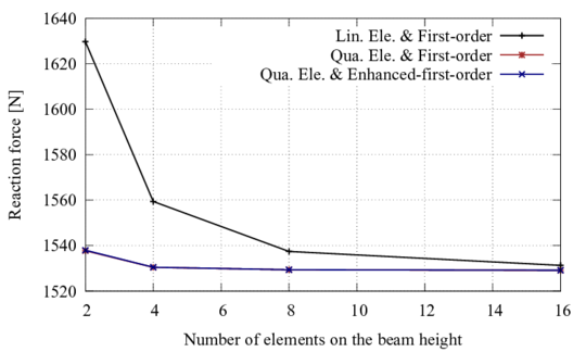
|
| Figure 37: Reaction force vs number of elements in Z direction for the different approaches. |
For the case of composite materials it is necessary make a difference between the results obtained for the homogenized composite ( macroscopic result), and the results obtained for the composite components in the RVE solution.
In Table 16 are shown the longitudinal and shear stresses for the composite obtained for the different approaches and meshes used on the beam. The macroscopic stresses values shown in the table correspond to the ones obtained in the Gauss point closest to point A. The composite stresses obtained for the QE&FO and QE&EFO cases are the same, as has been seen in Table 12. Figure 38 shows the longitudinal stress and Figure 39 the shear stress obtained for the composite. The curves show the stress obtained for the different approaches vs the number of element on the beam height. The composite stresses values obtained for QE&FO and QE&EFO are the same for all mesh analyzed because the EFO approach enriches the microscopic stress field but does not improve the macroscopic homogenized stress.
| Data | Composite [MPa] | Composite [MPa] | ||||
| LE&FO | QE&FO | QE&EFO | LE&FO | QE&FO | QE&EFO | |
| Macro1 | 185.54 | 221.36 | 221.39 | -25.19 | -9.21 | -9.21 |
| Macro2 | 218.02 | 238.29 | 238.29 | -15.02 | -4.17 | -4.17 |
| Macro3 | 235.96 | 247.13 | 247.13 | -8.17 | -1.98 | -1.98 |
| Macro4 | 245.71 | 251.59 | 251.59 | -4.27 | -0.96 | -0.96 |
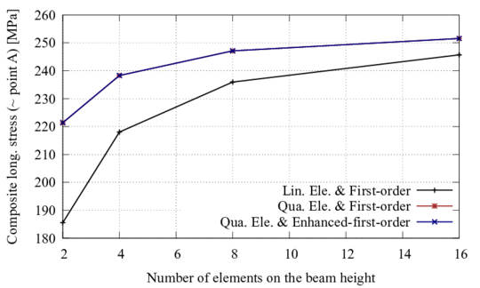
|
| Figure 38: Composite obtained close to point A for the different meshes and approaches used. |
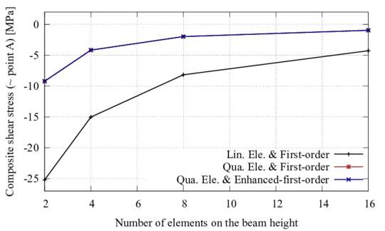
|
| Figure 39: Composite obtained close to point A for the different meshes and approaches used. |
The improvements on the microscopic results when an EFO approach is used can be seen in Figure 40. The microscopic stress fields shown in the figures correspond to the RVE of the macroscopic Gauss point closest to point A for the bean mesh Macro3. Figures on the left side present the longitudinal stress distribution obtained in the RVE for the fiber component while the right side shows the results obtained for the matrix component. The longitudinal fiber stress distribution for the FO approach is almost uniform for both kind of FE considered. While in the case of EFO approach the fiber stress distribution in the RVE is more realistic considering the bending macroscopic state. The classical linear distribution in the longitudinal stress expected for a bending load is achieved around the average value obtained for the FO approach. The stress distribution for the matrix present a similar behavior to the fiber component. It can be observed that the maximum stress for the fiber and matrix within the RVE are obtained in the Gauss points closest to point A, which is an expected result.
| ||||||||||||
| Figure 40: Fiber and matrix longitudinal stress field in the RVE of the Gauss point closest to point A for the mesh Macro3. |
To quantify the improvement on the microscopic solution due to the EFO approach, Table 17 shows the maximum values of the longitudinal stress for the fiber and matrix components within the RVE. These stress values are graphically represented in Figure 41a for the fiber material and in Figure 41b for the matrix component. From the figures is clearly seen that the response of components change when the approach is changed.
| Data | Fiber [MPa] | Matrix [MPa] | ||||
| LE&FO | QE&FO | QE&EFO | LE&FO | QE&FO | QE&EFO | |
| Macro1 | 454.56 | 543.31 | 616.13 | 11.11 | 11.18 | 14.10 |
| Macro2 | 534.71 | 584.90 | 622.41 | 11.69 | 12.01 | 13.67 |
| Macro3 | 578.97 | 606.60 | 625.56 | 12.23 | 12.46 | 13.25 |
| Macro4 | 603.02 | 617.54 | 627.07 | 12.53 | 12.68 | 12.98 |
10 Numerical comparison with other formulations
In the following chapter a comparison of the results provided by the homogenization approach presented in the previous chapter with other formulations is shown. The other two formulations used in the comparison are: a Micro model and the Serial-Parallel theory.
10.1 Introduction
The objective of these simulations is look into the strengths and weaknesses of the multiscale homogenization framework developed in this study. And, to known the computational cost required by the proposed formulation in comparison with other approaches used to analyze composite materials. The other formulations used for the comparison have been selected because they obtain the global behavior of the composite from the analysis of its microstructure. In the following, a brief description of each one of these numerical approaches is presented.
10.1.1 Micro models
In these models, the constituent materials forming the composite are modeled explicitly. Therefore, the response of the composite arises naturally. Each single material is modeled with its own constitutive law. These models are very powerful because they do not need to take any hypothesis on the microstructural behavior. However, as it will be shown, their biggest limitation is their computational cost and in most cases their use is not practical.
10.1.2 Serial-parallel mixing theory
The Serial-Parallel (SP) mixing theory could be defined as a phenomenological homogenization because it is based on the classical mixing theory. This formulation has been proposed by Rastellini et al. [4] and it assumes as principal hypothesis that the components of the composite behave as parallel materials in the fibers alignment direction and as serial materials in the orthogonal direction. The theory makes the composite behavior dependent on the constitutive laws of the component materials and of their morphological distribution inside the composite. The proposed composite constitutive model is based on the appropriate management of the constitutive models of component phases within a continuum framework by making use of suitable “closure equations” that characterize the composite micro-mechanics. For more details regarding the formulation, see Section 2.2.6 in Part I.
The potential of the SP approach is that predicts accurately the response of composites in the linear and non linear range (i.e. delamination failure) as has been proved in several papers [29,28,33,31,27,30,32]. For this reason, this theory has been selected for the comparison.
10.1.3 Homogenization approach selected
The first-order homogenization approach is used in the simulation because the aim of the comparison is to know the advantages and drawbacks of the general homogenization framework developed. Furthermore, the simulation is not looking for precision results on the microstructure, and it is conducted in the linear range.
10.2 Geometry and numerical models
A clamped beam with a vertical load at mid-span is the structure used to compare the theories described previously: micro model, serial-parallel mixing theory and first-order homogenization approach. Figure 42 shows the beam's geometry, supports and loads. A macro numerical model will be used to simulate the behavior of the structure with the different theories. In the case of the first-order homogenization approach another micro numerical model is necessary. The micro numerical model will have the internal structure of the composite.

|
| Figure 42: Geometric of the beam studied. |
10.2.1 Macro and micro numerical models
The macro FE model used is the half of the beam because the symmetry of the structure (see Figure 42). Figure 43 shows the macro numerical model with one of the meshes used. The finite element used is a first order hexahedron element. In order to obtain the real behavior of the structure with the FE model it is necessary to impose symmetric boundary conditions. The symmetry plane, the right face of Figure 43, normal to X-axis, and the X displacement is set to zero in this face. To simulate the fixed support, the nodes' movements in the left cross section are also restricted. The applied load is a Z direction fixed displacement of -0.1 mm in the rigth cross section nodes (symmetry plane).
As said before, to simulate the microstructure in the first-order homogenization a micro numerical model is required. The RVE's geometry chosen is a cube with unit length sides. The finite element used is the same than the macro numerical model. The different RVE models that will be used are shown in the Figures. 44 and 47.
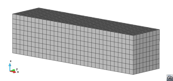
|
| Figure 43: Beam numerical model |
10.2.2 Simple materials and composite description
The simple materials in all studied cases are isotropic elastic materials. The composite material is a laminate. And, the laminate consists of several layers of material 1, called lamina 1 henceforth, and a combination of layers of material 2 (lamina 2) or material 3 (lamina 3). The volumetric participation of lamina 1 is always a 50%
Table 18 contains the mechanical properties of all the materials considered in the composite. In this table, is the Young's modulus, is the Shear modulus and is the Poisson's ratio. The “Color ref.” is the color used to represent the material in the RVEs, as it is shown in Figs. 44 and 47. The lamina 3 has the same properties as lamina 2, with the only difference of the shear modulus, which is reduced by 10. This is done to emulate the effect of a degraded lamina 2.
| Simple mat. | Color ref. | |||
| Lamina 1 | Black | 210 | 80.76 | 0.3 |
| Lamina 2 | Grey | 3.5 | 1.46 | 0.2 |
| Lamina 3 | White | 3.5 | 0.146 | 0.2 |
10.3 Comparison for several material configurations
In this section, several examples are presented to compare the behavior of the different theories. The result used to compare them is the reaction force, in Z direction, at the fixed support obtained for a fixed Z displacement applied at the symmetry plane (See Figure 42) .
10.3.1 Undamaged case
The undamaged case is the first one used to compare all theories. In this case the laminate contains 50% of lamina 1 and 50% of lamina 2, which properties are defined in Table 18.
The model using the SP mixing theory defines the composite material assuming that the parallel behavior is obtained in X and Y direction, while the rest of directions have a serial behavior. The homogenization formulation uses a RVE made with 8 elements that also contains 50% of lamina 1 and 50% of lamina 2. The RVE is shown in Figure 44. Finally, the micro-model is defined discretizing the different layers in which the laminate is divided.
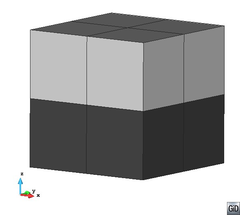
|
| Figure 44: RVE used for the undamaged case. |
A convergence analysis of SP and Homogenization theories has been made. The quantity of finite elements in the macro-model FE mesh has increased until the difference, between two consecutive results, is negligible. Figure 45 presents the results obtained for the different meshes analyzed. The micro-model used to compare the results obtained with the different theories has been made with 196608 hexahedron elements, which results in 648999 degrees of freedom.
The reaction force obtained with the SP theory is 905.9 N, with the first-order homogenization is 908.3 N and with the micro-model is 919.0 N. It can be concluded that the three theories provide almost the same result, as the difference between the reaction force value is lower than a 1% which is a really good result. Besides, all theories allow knowing not only the global performance of the beam analyzed, but also the specific response of each lamina to the loads applied.
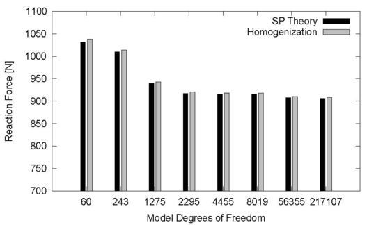
|
| Figure 45: Convergence analysis results. |
10.3.2 Global damage case
The objective for this example is to compare the responses obtained when one of the laminate materials suffers some sort of degradation. To analyze this problem, five different simulations have been performed in which the mechanical properties of one of the laminates is reduced. More specifically, the degradation is applied on the shear strength of lamina 2, which is reduced progressively until reaching the value of lamina 3 (see Table 18). Therefore, the new laminate consists 50% of lamina 1 and 50% of a new lamina that can be completely undamaged (properties of lamina 2) or with properties corresponding to 12.5%, 25%, 50% and 100% of damage (this last case, corresponds to lamina 3). The specific mechanical values considered are shown in Table 19.
| Property | 12.5% | 25% | 50% | 100% |
| 1.295 | 1.131 | 0.803 | 0.146 | |
| 3.5 | 3.5 | 3.5 | 3.5 |
The composite is simulated with the SP mixing theory and with the first-order homogenization, using the same material characterization and RVE that were used in the undamaged case. Figure 46 shows the results obtained for the conducted simulations. This figure shows that, as it is expected, the results obtained for both theories are again exactly the same. The results obtained also show that as the shear stiffness of one of the layers is reduced, the global stiffness of the beam decreases. This effect can be understood as a delamination failure, as has been previously shown by Martinez et al. [28,31]. Results also show that the reduction of global stiffness of the beam is not linear with the reduction of the shear strength of one of the laminas, being larger as the layer stiffness gets smaller.
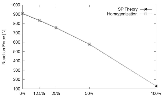
|
| Figure 46: Reaction force obtained in the global damage case. |
10.3.3 Local damage case
In this example, the objective is to compare the responses obtained when material damage takes place, not in all layers, but just in some of them. The composite considered has always 50% of lamina 1, and a 50% of lamina 2 (undamaged and damaged). It is assumed, like in the previous case, that a totally damaged lamina 2 is numerally represented by the lamina 3. The comparison is made for the cases in which there are 0%, 12.5%, 25%, 50% and 100% of layers damaged. The simulation corresponding to 0% and 100% damaged have been already conducted in two previous simulations. The simulations corresponding to intermediate cases have been studied with the three methods being compared in this chapter: first-order homogenization, SP and a micro-model.
For SP theory, the composite is obtained combining two different laminates with the SP formulation. One laminate has 50% of lamina 1 and 50% of lamina 2 and the other laminate has 50% of lamina 1 and 50% of lamina 3. The volume fraction of these laminates in the composite depend in the amount of layers assumed to be damaged. For the homogenization approach, the amount of layers damaged is represented with the RVE. Figure 47 shows the RVEs considered to account for 50%, 25% and 12.5% of damaged layers, respectively. In this figure, the darker elements correspond to lamina 1, the light-grey elements correspond to lamina 2 (undamaged) and the white elements correspond to lamina 3 (damaged). Finally, the micro-model has been simulated discretizing each one of the lamina of the beam.
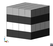
|
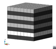
|
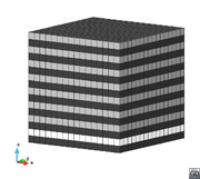
|
| Figure 47: RVEs containing 50%, 25% and 12.5% of damaged layers. | ||
Figure 48 presents the results obtained with different simulations performed. This figure shows that for the extreme cases, this is for 0% or 100% of lamina 3, the results obtained with different theories are almost equal. However, the results obtained when there are some layers damaged do not have the same agreement, especially when comparing the results obtained with the SP theory with the ones obtained with the homogenization method or the micro-model. While the decrease in the resultant reaction force with the SP theory is equal to the one obtained in the case of considering global damage (see Figure 46), this decrease is substantially larger when considering the homogenization method or a micro-model. These two theories provide nearly the same results.
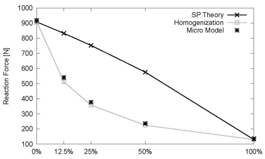
|
| Figure 48: Reaction force obtained in the local damage case. |
The explanation for the difference in the response obtained for the different models is obtained from the models themselves. The serial-parallel theory obtains the response of the composite assuming certain iso-stress and iso-strain boundary conditions that regularizes the response of the material if it is defined with several laminates. Therefore, the response of the structure and the result obtained is similar to the one obtained when this damage was present in the whole structure. On the other hand, with the homogenization and the micro-model theories, the damaged layer is discretized specifically and it is possible for the simulation to capture the dislocation that takes place, as it is shown in Figure 49 for the three cases considered. This dislocation is the responsible for the drop of the stiffness and the fast decrement on the value of the reaction obtained.
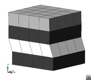
|
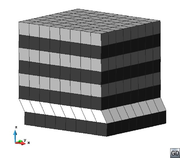
|
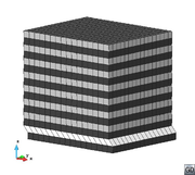
|
| Figure 49: RVEs with 50%, 25% and 12.5% of damaged layers under load. | ||
10.3.4 Local damage case in a localized region of the beam
At the light of previous results one may think that the SP theory is not capable of representing delamination processes. In this example it is shown that under some circumstances this simulation is possible. Here, the beam has been simulated with two different laminates. The central band contains 50% of lamina 1 and 50% of lamina 3 (damaged); while the rest of the beam is simulated with 50% of lamina 1 and 50% of lamina 2. Figure 50 shows the FE mesh of the beam macro-model. This example is simulated with the SP and the homogenization theory. The homogenization theory uses the RVE shown in Figure 44.
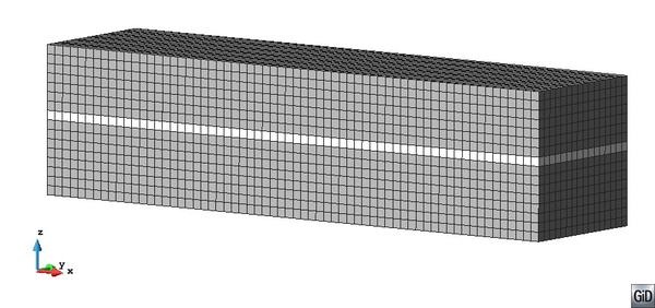
|
| Figure 50: FE mesh of the macro-model of the beam with two laminates. |
In this case, the reaction force obtained is exactly the same for both, the SP and the homogenization models: 663.9 N and 666.4 N, respectively. This example shows that the SP theory is capable of providing the same results as the homogenization theory when the response of the RVE fulfills the parameters in which is based the SP theory: iso-strain and iso-stress behavior. On the other hand, if the RVE does not fulfill this behavior (i.e. there is a dislocation in it), the SP theory is not capable of predicting accurately the material response, as it was shown in previous example.
10.4 Run times and memory used
One of the main drawbacks that has a homogenization approach nowadays is its computational cost. Therefore, in order to know the performance of this formulation it is necessary not only to compare the results obtained with it, but also to compare the computational cost in terms of time and memory requirements.
To do these comparisons, in the case of the computational homogenization, two different strategies have been considered. In the first one, the mechanical properties of the composite (stiffness matrix) are calculated at the beginning of the analysis, and these properties are used afterwards during the complete of the simulation. This case is named H-OneRVE. The other case corresponds to analyze the RVE each time that it is necessary to know the stress provided by the RVE for a given strain value. This case is named H-AllRVE. If the problem is linear, the results obtained in both cases are the same. However, in a non linear case, it is necessary to simulate the problem with an H-AllRVE strategy in order to capture properly the non linear response of the material.
| Item | Micro Model | H-OneRVE | H-AllRVE | SP Theory |
| Real Time [Min:Seg] | 6:46 | 0:01 | 2:27 | 0:02 |
| CPU Time [Min:Seg] | 8:44 | 0:03 | 9:31 | 0:17 |
| Memory [Mbytes] | 2690,00 | 7,45 | 7,45 | 15,82 |
| Reaction Force [N] | 236,09 | 224,69 | 224,69 | 576,68 |
Table 20 shows the computational times and memory required to conduct the simulations with a localized damage of a 50% The real time and cpu time are discriminated because part of the FE code used is in parallel. The results show that the CPU time in the Micro model and H-AllRVE are comparable. But, the CPU time of the H-OneRVE and SP theory are significantly better. Therefore, in terms of computational time, it is feasible to conduct a simulation with a homogenization approach, as well as with the SP theory. However, this simulation must be kept in the linear range. If the simulation is non linear, the H-AllRVE strategy must be used, which makes the SP theory the only feasible option in terms of computational time unless some non-linear strategy is developed to minimize the number of times in which the RVE has to be solved.
The main difference between the micro-model and the homogenized model is found in the memory requirements. While the computational time of the H-AllRVE and the micro-model are equivalent, the amount of memory required by this last one is substantially larger (360 times larger). This difference is found because the memory used is proportional to the FE mesh size of the numerical model and, while the micro-model has to solve a problem with a very small discretization, the homogenization framework only requires memory for the macro-problem and the RVE that is being solved. This difference makes unbearable solving large problems with micro-models and makes feasible using homogenization methods, even if the problem is in non linear range.
11 Non-linear extension proposed for multiscale methods
Most of the work on FE2 multiscale procedures are done on analyzing the numerical performance of RVE [143,144] or on connecting different scales [124]. In general, in this kind of homogenization methods the elastic properties of the microstructure are obtained solving the microstructural problem at the beginning of the structure problem. The main drawback of homogenization methods is their computational cost for a non-linear analysis because it is required solving the RVE in every integration point at the macrostructural problem, and for every time step, in order to know the non-linear limit and then the behavior of the microstructure in non-linear range. Non-linear performance has also the problem that the dissipated energy of both scales is not always related [145].
In order to improve the computational cost of the multiscale homogenization some strategies use model-order reduction techniques [146,147,148]. These methods use the Proper Orthogonal Decomposition (POD) to obtain the reduced set of empirical shape functions. Besides, [148] proved that the common approach of replacing the non-affine term by an interpolant constructed taking only POD modes arrives to ill-posed formulations. An enriched approximation space with the span of the gradient of the empirical shape functions is proposed to avoid this ill-posedness. However, these kind of procedures do not solve the complete structure.
Because of this, in the following to overcome this major drawback, this chapter presents a new procedure to reduce computational cost of multiscale simulations [120]. The chapter looks also into the problem of localization and energy dissipation across the scales, as the proposed method must be consistent [149]. In the following the formulation and algorithm schemes of the proposed procedure are described.
11.1 Introduction
The main advantage of the FE2 method compared to a micro model is the reduced computer memory requirements. To solve the same problem, the amount of memory required by the classical FE micro model method is substantially larger than FE2 procedure [119]. This difference is found because the memory used is proportional to the FE mesh size and, while the FE micro model has to solve a problem with a very small discretization, the FE2 procedure only requires memory for the macrostructural problem and the RVE that is being solved. However, if the material reaches non-linear behavior, the computational cost of FE2 method becomes as large as the one required by the micro model case, as the RVE has to be solved for each integration point when a real structure is solved. Because of this, a new Non-Linear Strategy (NLS) is proposed in this work.
Continuum mechanics establishes the limit between linear and non-linear performance of materials using a comparison criterion that compares a given combination of stresses with a threshold value (Von-Mises, Mohr-Coulomb, etc.). This approach cannot be used in an homogenization double scale solution directly as different strain-stress states may lead to different failure modes of the composite.
A possible solution is to analyze the RVE at every time step. However, as has been already stated, this is extremely expensive and very ineffective, because the structural non-linear behavior often occurs in a small part of its domain.
The non-linear strategy developed consists in the definition of a comparison criterion, based on the macrostructural deformation of the Gauss point, but takes into account that the RVE failure takes place in a small part of the domain. In the following section it is explained in detail. It has to be noted that the procedure proposed has been developed for a first-order homogenization approach. Further study will be required if it wants to be extended to the enhanced-first-order homogenization approach, as in this case it should account not only for the macrostructural Gauss point deformation, but also for its gradient.
11.2 General concepts of the proposed approach
Here is proposed to develop a comparison function that looks a maximum level of an elastic energy density that can be applied to the RVE before its failure. This is done with the definition of an activation function for each single integration point at the structural scale. It is important to remark that the proposed approach does not use a model reduction strategy, instead it is solving the actual structure, but only when it is strictly necessary.
The NLS is composed of two different procedures, a non-linear activation function and a smart first step calculation. In the following are defined both of them.
11.2.1 Non-linear activation function
The definition of a Non-Linear Activation Function (NLAF) is based on the fact that any given material begins its non-linear performance when a single particle of the material reaches its stress threshold. The objective of the NLAF is to know whether any material point of the RVE has reached its non-linear limit using homogenized variables.
To do so, it defines a function f that relates the elastic energy density () of an integration point of the RVE with the maximum elastic energy () that can be applied to this material point, before reaching the non-linear range. Therefore, f is defined as
|
|
(11.1) |
In other words, f provides a value of how far is a material point in the microstructure to reach the non-linear state.
In order to know how far is the whole RVE to reach the non-linear performance, it is necessary to use the information obtained for all the integration points of the RVE and transform it into a single representative number. This is done with the assumption stated before that the failure of the macrostructure will start when the first integration point of the microstructure fails. Therefore, the parameter of the RVE corresponds to the maximum f value of all integration points of the RVE. Then
|
|
(11.2) |
where the overline at the variables refers to the structure scale or homogenized variables. Finally, the limit elastic energy density at the macrostructure scale is obtained with the following expression
|
|
(11.3) |
where is the elastic energy density for the strain state used to calculate . The process described can be schematized as it is shown in Figure 51.

|
| Figure 51: Non-linear activation function scheme. |
The NLAF is defined as
|
|
(11.4) |
where is the elastic energy density of the macro structural integration point, which is calculated in each load step of the simulation.
The NLAF previously defined is only valid for the strain state used to calculate (see 11.3). If the strain state varies, it may also change the non-linear failure mode and, therefore, the limit elastic energy density calculated may be no longer valid. Therefore, 11.4 is valid while the strain state in the material remains proportional to the one used to obtain . To quantify this proportionality the next expression is proposed
|
|
(11.5) |
where the subscript refers to the current i-nth deformation state and is the norm's mathematical symbol. In case this proportionality is lost, it will be required to calculate again the new limit elastic energy density of the RVE. This is summarized in the following flow diagram (see Figure 52).

|
| Figure 52: Non-linear strategy algorithm scheme. |
It can be easily seen that with the proposed procedure the RVE must be solved for each macro integration point on the first time step, in order to calculate the elastic energy density limit using 11.3. Afterwards, it only will be necessary to solve the RVE again if the strain state of the integration point becomes non proportional to the calculated originally or if the NLAF is not satisfied, which means that the RVE becomes non-linear. Therefore, if only few elements of the structure reach the non-linear state, only these elements will have to be solved in the non-linear analysis.
11.2.2 Smart first step
As said before, at the beginning of the analysis it is required to solve the RVE for every single integration point of the macrostructure to obtain its . This calculation process can be extremely expensive in terms of computational cost.
In order to reduce this computational cost, it is proposed a Smart First Step (SFS) strategy. This strategy consist in solving the RVE only if the deformation applied to it is different to all other deformation states considered previously. Therefore before calculating the of the RVE, the SFS procedure compares the deformation between the current and the all previous integration points already calculated (see 11.5). If the SFS finds one comparable strain state, the current RVE takes the values of the RVE already solved. If none of the previous microstructures solved have a comparable state, the actual RVE is calculated. Figure 53 shows the scheme of the described algorithm.
It will be shown, in the validation examples, that this procedure reduces significantly the computational cost of the first step load in the simulation.
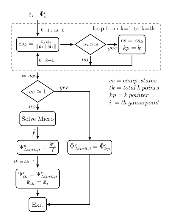
|
| Figure 53: Smart first step algorithm scheme. |
11.2.3 Numerical homogenized tangent constitutive tensor
The proposed NLS has been implemented in PLCd [9], a parallel finite element code that works with 3D solid geometries (see Appendix B.5). In the code, a Newton-Raphson scheme is adopted to solve the non-linear problem. To facilitate the convergence of the whole problem, the tangent constitutive tensor at the integration point is necessary to obtain the global tangent stiffness matrix.
A perturbation method is used to obtain a numerical approximation of the homogenized tangent constitutive tensor of the RVE in the integration point. The method implemented is analogous to the one proposed by Martinez et al. in [33] (see Section B.5.2 in Appendix B.5). Being the only difference that in current procedure the perturbations must be applied on the RVE instead of applying them to a constitutive equation. The small perturbations () are applied to the homogenized or structural strain vector. The RVE is solved times and as result gives the stress vector . Therefore, the columns of the tangent constitutive tensor for the RVE can be obtained as
|
|
(11.6) |
The calculation of the tangent stiffness tensor is necessary to obtain a good convergence of the problem but it is computationally expensive. This shows again the necessity to reduce the number of times in which this calculation is performed, and proves the necessity of having a non-linear strategy to conduct the simulation.
11.3 Energy dissipation in a multiscale analysis
The solution of material non-linear problems with a numerical double scale homogenization procedure not only should be affordable computationally, but the results obtained in the non-linear process must be also correct. Therefore, the procedure must dissipate the same energy in both scales. In order to conserve the dissipated energy through the scales, the following methodology is proposed.
11.3.1 Fracture energy
Fracture mechanics presents the fracture energy per unit of area, , as a property of the material. This energy can be calculated as
|
|
(11.7) |
where, is the energy dissipated by the fracture at the end of a quasi-static process, and is the total fractured area. This fracture energy is the link between the fracture mechanics and the constitutive model based on classical solid mechanics. The constitutive model must satisfy:
- The good representation of behavior of a set of points inside of a finite domain.
- The same energy dissipated by the total volume as the one dissipated by the solid in the real fracture process.
Considering a simple tensile test, the constitutive model must verify the following condition of dissipation
|
|
(11.8) |
where is the maximum specific energy dissipated by the constitutive model. Equation (11.8) states that the energy delivered to the tensile test must be equal to the energy dissipated by the constitutive model. In solid mechanics, the dissipation phenomena is located in a volume that can be represented as , where is a fracture length. For FE method the localization phenomena in one strip of finite elements is sought, therefore is commonly approximated by some reference length of the finite element. This length is a parameter that accounts for the amount of energy dissipated by the fractured material. Replacing the volume in 11.8 the following expression is obtained
|
|
(11.9) |
From 11.9 the relation between the material parameter and the specific energy dissipated is found
|
|
(11.10) |
11.3.2 Localization at the microstructural scale
In multiscale procedure, the specific energy at the macro structural scale is obtained as
|
|
(11.11) |
where the index is used to reference the microstructural scale variables.
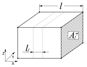
|
| Figure 54: Representative volume of the subscale. |
Taking the same consideration than macroscale solid behavior, now the dissipation phenomena is located at microstructural level (see Figure 54). In such case, we have the following dissipated equation
|
|
(11.12) |
where, is the RVE cross section area, is the length in normal direction of and is the fracture length at the microstructure (RVE). With 11.12 is possible to obtain the specific energy dissipated at the microstructural scale level as
|
|
(11.13) |
Equation 11.13 shows the relationship between the and which ensures to dissipate the same energy by the solid mechanics, using a multiscale method, than the one obtains with a tensile test. The validity of this relation is proved in the following example.
11.3.3 Validation example
A simple tensile numerical test over a material sample is simulated. The objective of this example is to analyze the objectivity of the response obtained using the proposed FE2 method. The same test using a classical one scale FE method is also solved for comparison purposes. The geometry, the supports and the displacements scheme of the simulated structure is presented in Figure 55. The applied fixed displacement is represented by the arrows in the figure.

|
| Figure 55: Structure simulated in the tensile test. |
11.3.3.1 Material
The simple material used in the tensile test takes the properties shown in Table 21. The constitutive model chosen is an explicit scalar damage model with exponential softening [150,151]. For this particular case, where the stress state is uniform and there is only one simple material, and in order to help the localization of the softening problem, the elastic limit is increased in some elements (drawn with gray color in Figure 56) up to a value of .
| Properties | ||||
| Values | 100 | 0 | 100 | 20 |
11.3.3.2 FE meshes
The finite element used to solve the problem is a first order hexahedron element. The example is solved for different combinations of finite element meshes. Figure 56 shows the different mesh sizes used in the simulation. The left side of Figure 56 shows the three different meshes used for the structural scale. The mesh Macro1 has 10 finite elements, the mesh Macro2 has 84 elements and finally the mesh Macro3 has 656 elements. On the other hand, the right side of Figure 56 shows the two different meshes used for the microstructural scale. The mesh Micro1 has 125 finite elements and the mesh Micro2 has 729 elements.
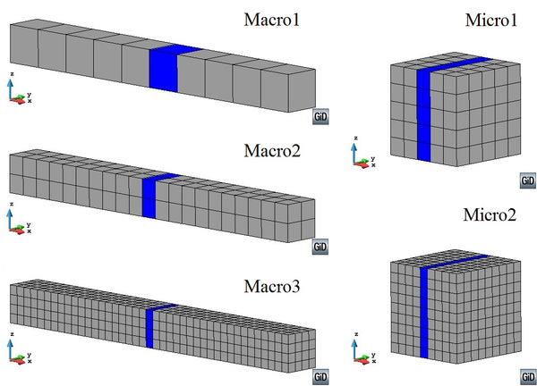
|
| Figure 56: Different meshes used in the tensile test. |
11.3.3.3 Results
The results obtained with the different mesh combinations are shown graphically in the Figure 57. As can be observed from the figure, the results are equal for all combinations, and for both methods.
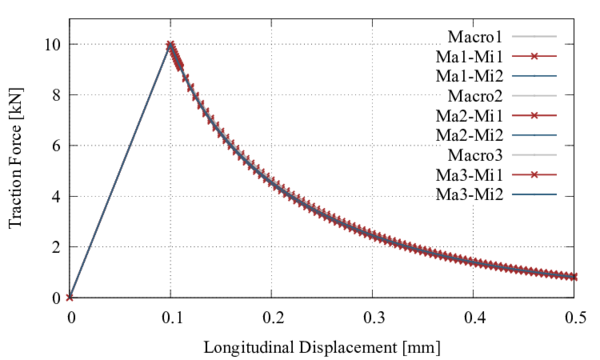
|
| Figure 57: Traction force vs displacement curves obtained in the tensile test. |
For the case considered, it is possible to validate the numerical results with analytical calculations, knowing the area of the specimen, the Young's modulus and the maximum tensile stress that can be applied, the maximum load and displacement in the beam is
|
|
It is also possible to calculate analytically the dissipated energy at the end of the test as
|
|
If this energy is calculated from the numerical models, the following table is obtained:
| Energy | Macro1 | Macro2 | Macro3 |
| One scale | 1.728 | 1.737 | 1.748 |
| Micro1 | 1.752 | 1.741 | 1.777 |
| Micro2 | 1.713 | 1.761 | 1.812 |
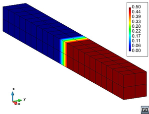
|
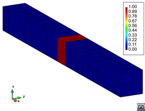
|
| Figure 58: Macrostructural results obtained at the end of the tensile test. | |
The localization of non-linear phenomena in one strip of finite elements at the structural scale is shown in the Figure 58, for the analysis made with Macro2 mesh. This figure shows that damage is concentrated in the central zone of the material sample, and therefore, the displacement too. In the proposed multiscale method the localization phenomena must be observed also at the microstructural scale. As an example, Figure 59 shows the microstructural displacement and damage obtained at the end of one tensile numerical test. In the figure can be observed that both results are localized in one strip of finite elements in the RVE meshes.
| |||||||||
| Figure 59: Microstructural results obtained at the end of the tensile test. |
11.4 Numerical examples of non-linear analyses
11.4.1 Tensile test of a plate with a hole.
The objective of this example is to show the performance of the NLS developed, as well as to analyze the failure of the structure localizes in a strip of elements. The test is a tensile test made on a plate with a hole in its center. Due to the symmetry of the geometry and of the load applied, only a quart of the real structure is simulated. Figure 60 shows the modeled geometry, the supports and the displacements scheme in the numerical model. The applied fixed displacement is represented by the arrows in Figure 60.

|
| Figure 60: Simulated structure of the plate with a hole. |
11.4.1.1 Material
Table 23 shows the properties of the simple material used. The constitutive model of the material is the same (explicit scalar damage) that has been used in the previous validation example 11.3.3.
| Properties | ||||
| Values | 100 | 0.15 | 100 | 10 |
11.4.1.2 FE meshes
To analyze the response's objectivity in the test, two finite element meshes have been used for the macroscopic model. Figure 61 shows the mesh sizes employed. Mesh1 has 360 finite elements while Mesh2 is more dense and has 2880 elements. The microstructural model and finite element meshes are the same than the ones used in previous validation example 11.3.3.

|
|
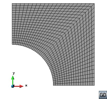
|
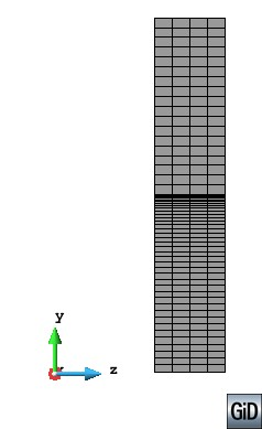
|
| Figure 61: Different meshes used in the plate with a hole. | |
11.4.1.3 Results
Figure 62 shows the traction force vs displacement curves obtained for the different mesh combinations. This figure shows that the results are almost equal. Therefore, the result obtained with the proposal method is mesh independent. The curves show than the maximum force does not pass of 80 KPa and it is obtained for an applied displacement of 0.08mm.
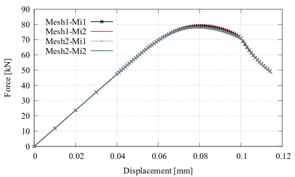
|
| Figure 62: Forve vs Displacement for the plate with a hole. |
The dissipated energy for the different mesh configurations used in this example is shown in Table 24. From the Table 24 can be observed than the worst difference between two results is less than 2%
| Energy | Mesh1 | Mesh2 |
| Micro1 | 3.152 | 3.135 |
| Micro2 | 3.192 | 3.169 |
To fully understand the behavior of the structure under the applied load several figures for different load state are presented. Figure 63 and Figure 64 show the results obtained for Mesh1 and Mesh2, respectively. In the figures, strain and stress in Y direction and scalar damage are presented for four different fixed displacement steps.
| ||||||||||||||||||||
| Figure 63: Results obtained in the plate with a hole to Mesh1. |
The figures show how at the beginning of the test (label a) d=0.05mm), the maximum strain and stress are located at the inner border of the hole. Then, the non-linear process starts there and, as a consequence, the damage increases in that zone. Due to constitutive model used, when the damage increases in the material the stress decreases. As the applied displacement continues increasing, the structure transfers the load to non damaged zones. Therefore, the zone with maximum stress moves from the inner border to the central part and the strain and damage move on as a constitutive response. At the end of the test (label d) d=0.11mm in the figures), the maximum stress is located in the right external border of the plate. It is important to mention that during the test, the stress in the structure never takes values over the limit imposed (see Table 23) as can be observed in Figures 63 and 64. Finally, the figures show how the model is capable of localizing all damage in a single strip of finite elements.
| ||||||||||||||||||||
| Figure 64: Results obtained in the plate with a hole to Mesh2. |
11.4.1.4 Computational times
To show the advantage of using the NLS proposed, in comparison with a full classical FE2, the calculation times are presented herein. A full FE2 solves the microstructural problem for every integration point of the structure, and for every time step. This procedure does not distinguish between linear range and non-linear range.
Tables 25 and 26 present the calculation times required to solve the shown example in the same desktop computer, an Intel CoreTM i7-2600 CPU @ 3.40GHz with 8GB of RAM. The tables show the times used by the FE2 and by the FE2 with the NLS incorporated. The speed ratio column has the relation times between both methodologies.
Table 25 has the total real times necessary to complete the numerical test, up to d = 0.115mm, for all mesh configurations. The speed ratio variable shows that the advantage of using the developed strategies increases specially when the size of the macrostructure's mesh increases. This is an expected result because, in larger meshes, the proportion between linear and non-linear elements becomes also larger.
| Model | FE2 | FE2+NLS | Speed ratio |
| Mesh1-Micro1 | 1:21:53 | 0:28:19 | 2.89 |
| Mesh1-Micro2 | 8:41:19 | 3:10:44 | 2.73 |
| Mesh2-Micro1 | 11:19:49 | 2:29:28 | 4.55 |
| Mesh2-Micro2 | 76:40:33 | 18:39:33 | 4.11 |
On the other hand, it is important to mention that when a RVE becomes non-linear, its computational cost is more expensive than when it is linear. This is because, besides the possible iteration required by the RVE to obtain the correct non-linear solution, the estimation of the tangent constitutive tensor by perturbation method requires to solve the RVE six more times (see Subsection 11.2.3).
Consequently, when the number of non-linear elements in a problem increase, the efficiency of the proposed method decreases. For the analyzed example, if the simulation is stopped at the maximum admissible force in the structure (around d=0.08mm in Figure 62) which probably the most interesting value for an engineer, the speed ratio would be better. To prove this, let's consider the Mesh2-Micro2 simulation. In this case, when the maximum load is applied (d=0.08mm) there are only 392 elements in non-linear range, instead of 576 elements for d=0.115mm, and therefore at this load step the speed ratio is of 7 instead of 4.11.
This simulation is also used to validate the effect of the Smart First Step procedure. To do so, Table 26 shows the computational times consumed for the first step in each one of the simulations conducted. The times shown prove that using SFS strategy improves highly the computational efficiency also for small mesh sizes, as speed ratio variable shows. The table also shows that the number of RVE solved by the SFS is independent of the mesh used in the microstructural problem.
| Model | without SFS | with SFS | Speed ratio | ||
| Time | RVE solved | Time | RVE solved | ||
| Mesh1-Micro1 | 0:17.9 | 2880 | 0:01.0 | 151 | 17.9 |
| Mesh1-Micro2 | 1:48.3 | 2880 | 0:06.5 | 151 | 16.7 |
| Mesh2-Micro1 | 2:12.0 | 23040 | 0:02.6 | 303 | 50.8 |
| Mesh2-Micro2 | 14:05.9 | 23040 | 0:12.5 | 303 | 67.7 |
11.4.2 Industrial Component
In order to validate the efficiency obtained with the NLS when it is applied to the solution of a real structure, in the following is included the non-linear simulation of an structural component. In this case, the structure selected for analysis is the industrial component shown in Figure 65. The geometry of this engine stiffener has been proposed in the framework of M-RECT Project. The stiffener is linked on one side to the gearbox, and on the other side to the engine. This component has the objective of improving the connection between engine and gearbox, as well as changing the dynamic properties of the overall structure.
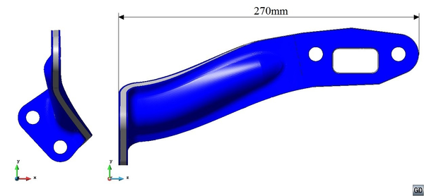
|
| Figure 65: Engine stiffener part. |
11.4.2.1 Materials
The material that will be used for the stiffener, different from the one used in M-RECT, is a laminated thermoplastic composite. Therefore, the material properties vary through the laminate thickness and respect to the laminate's reference direction. The composite is made with three orthotropic sheets (see Figure 65). The two external sheets (drawn in blue) have a thickness of 1.5mm each one and, the core sheet (drawn in gray) has a thickness of 5.5mm.
The external laminae is composed by carbon fibers in an epoxy matrix. The periodic microstructure of the external sheets can be represented by the RVE shown in the Figure 66. The laminate has a 40% of cylindrical long fiber volume.
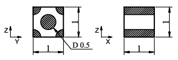
|
|
| (a) b) Mesh used in the RVE | |
| |
| Figure 66: Geometry and mesh of the RVE used in the external sheets. | |
The matrix is an isotropic material, simulated with an explicit scalar damage constitutive model with exponential softening (resin epoxy HSC Epikote 4652). The long fiber is modeled with an elastic constitutive model (Grafil TR30S 3K carbon fiber). The properties of these simple materials are shown in Table 27 [32].
| Material | ||||
| Epoxy matrix | 4.52 | 0.36 | 68 | 780 |
| Carbon fiber | 235 | 0.21 | 4410 | - |
Finally, the FE mesh employed to analyze the RVE is shown in Figure 66. The mesh uses 1464 first order hexahedra finite elements.
On the other hand, the core sheet of the engine stiffener is a TenCate commercial product, Cetex TC1200 PEEK 5HS LAMINATE. The properties of this material have been obtained from TenCate website [152] and are shown in Table 28. For the simulation, the core material is modeled using an elastic constitutive model.
| Propertie [GPa] | (In plane) | ||
| TenCate lamina | 56.1 | 55.6 | 4.5 |
11.4.2.2 Mesh and boundary conditions
Figure 67 label a) shows the mesh used to simulate the engine stiffener. The mesh has 355.302 first order tetrahedra finite elements. The external laminae requires 108.041 elements while the core lamina has 247.261 elements.
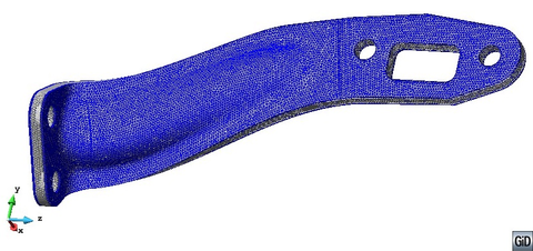
|
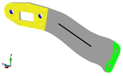
|
| (a) b) Nodes restricted and laminate's reference direction | (b) Mesh and boundary conditions used in the engine stiffener. |
| Figure 67 | |
The nodes that will be restricted and the laminate's reference direction are shown in Figure 67 label b). The nodes with green color are over the face in contact with the gearbox. These nodes have a zero movement restriction in all directions. On the other hand, the nodes drawn in yellow are on the face in contact with the engine. In this case, the restriction on these nodes is a fixed displacement in X direction. The laminate's reference direction is the long fiber longitudinal direction in the external laminae.
11.4.2.3 Results
The analysis conducted on the first step to evaluate the elastic energy density available in each integration point allows defining a “possible damage” map of the structure, as it is shown in Figure 68 label a), where is presented. The blue zones in the external sheets have an near to zero, which means that in these zones the relation between the elastic energy density required by the load, , and the available elastic energy density in the material under that load, , is very small. On the other hand, regions with values near to one can be defined as critical zones, as in these is very close to . Therefore, these zones are the regions where non-linear process has more possibilities to start. In this example, the SFS has required analyzing 6.514 RVEs to determine the threshold functions of the whole structure. This quantity represents only the 6% of the elements on the external laminae.
The numerical simulation has been stopped for a fixed X displacement of 1.36mm. The homogenized stress at the end of the analysis in the laminate's reference direction is shown in Figure 68 label b). From the figure it is observed that the maximum absolute stress is a compressive stress and it is located near to the face in contact with the gearbox. The maximum tensile stress is located in the same region but in the opposite external sheet.
Figure 68 label c) shows the scalar homogenized damage at the end of the test. The damaged area shown in figure has a relation with the previous results presented. It is on the maximum compressive stress zone (see label b)) and it is a critical zone in Figure 68 label a).
To understand the internal structure behavior in the damaged zone it is necessary to observe the mechanical performance of the most damaged RVE. In current simulation the RVE selected is the one with the maximum homogenized damage, in the engine stiffener mesh (see Figure 68 label c)). Figure 69 shows the results obtained for this RVE. This shows the stress in the RVE's local X axis at the beginning (label a) at first step) and at the end (label b) at last step) of the test. The shear stress in XY and YZ direction is also shown in the figure for the first step of the analysis. Finally, the matrix scalar damage variable in the RVE is shown for the last step.
From Figure 69 can be observed that X compression stress is the dominant state in the RVE but, its failure is produced by shear in the matrix material. In order to account for the high strength threshold of the carbon fiber (see Table 27), and to reduce computational cost, this material has been simulated with an elastic constitutive model. Figure 69 shows that this assumption is correct, as the maximum fiber stress reached in the analysis (label b) at last step) is far away of its strength threshold as it was expected.
The Figure 69 shows that the external sheet has interlaminar delamination in the damaged zone (see Figure 68 label c)). It is important to stand out that although the damage in the matrix is located in a small zone its global effect is meaningful. Figure 68 label c) shows that some elements have lost about 75% of its original load capacity.
This example has shown that it is possible to solve real problems with a non-linear homogenization scheme. However, to see the advantages of the proposed NLS procedure, it is necessary to analyze the computational times required by the simulation, these are shown in Table 29. The FE2 computational time has been evaluated based on the time required to solve one RVE and the number of steps and iterations required by the simulation. Table 29 shows that a FE2 has a computational cost that makes unfeasible these sort of simulations. In current case, the simulation requires more than 32 days and 14 hours to be completed. The proposed method has a really good computational time, less than 12 hours, and it is capable of speeding up the process at a speed ratio of 67.4. This implies a reduction of more than a 98% of the computational time required to conduct the calculation. In other words, it makes feasible a numerical analysis that was previously unfeasible.
| Methods | FE2 | FE2+NLS | Speed ratio |
| Time [hs:min] | 782:46 | 11:36 | 67.4 |
12 Numerical Homogenization. Concluding remarks
The multiscale homogenization framework proposed in Part 6 of the dissertation, which is described in detail in Chapter 9, has been proved a competitive alternative to model three-dimensional composite structures. An extension of the first-order homogenization approach developed has been proposed to consider high-order effects in the microstructure. The called Enhanced-first-order homogenization presented in Section 9.4 preserves a classical first-order BVP at the microstructure scale but also at the macrostructure scale. Therefore, with this new approach bending effects can be seen in the microscopic scale without increase the complexity of the macroscopic formulation and its computational implementation. However, there is no improvements in the macrostructure solution considering the one obtained with the first-order homogenization approach, as has been proven in the numerical example present in Section 9.8. The elimination of redundant unknowns implemented, for both cases of homogenization approaches developed, to solve the microscopic BVP through a cubic RVE has proven to be an efficient option to satisfy the boundary conditions.
For linear analysis, the comparison presented in the Chapter 10 proves that the multiscale homogenization has many advantages over other theories, such as micro models or the SP theory, as it is capable of capturing complex responses of the material (such as dislocations) with an affordable computational cost. The homogenization approach can represent accurately effects such as a local damaged lamina because the internal structure of the composite is physically modeled in the RVE. The SP theory cannot account automatically for such effects, unless they are present in the whole finite element, as has been shown in the examples presented in Sections 10.3.2 and 10.3.4. However, the main advantage of the SP theory is that it is capable of conducting non-linear analysis without increasing substantially the computational cost of the simulation.
The comparison of the computational cost presented in Section 10.4 by the different formulations has shown that, in terms of computational time, the cost of the first-order homogenization for elastic simulations that solve the RVE only at the beginning to characterize the material, and the SP theory is comparable. Besides, this computational cost is substantially lower than the one required by a micro model or for non-linear simulations conducted with a classical FE2 homogenization framework. However, the main difference between the full FE2 homogenization approach and the micro models is found in the memory required by the simulation, being the cost of this last one 360 times larger.
A proposed extension to non-linear range of the FE2 computational homogenization is proposed and presented in Chapter 11. The developed formulation uses a non-linear activation function defined in the structural scale that is obtained by solving the microstructure scale. The activation function predicts if a material point (or integration point) in the structure is in linear or non-linear range. Therefore, the approach proposed only analyzes the non-linear integration points by solving the microscopic BVP using the RVE. Section 11.2 shows the formulation developed to obtain the non-linear strategy proposed in this study. Besides, a smart first step had to be also developed to obtain in an efficient way the activation function.
The purpose of the non-linear procedure developed is to solve non-linear problems, and the first requirement to meet is conserve the dissipated energy through the scales. Section 11.3 describes in detail how the fracture length concept applied to one scale continuum mechanics is extended to multiscale homogenization approach. It is shown that the non-linear formulation presented is energy consistent and mesh independence at the macroscopic and microscopic scale.
The main objective of the proposed non-linear strategy is to reduce significantly the computational times requested by a multi-scale approach. The plate with a hole example presented in Section 11.4.1 shows how the computational times are reduced around four times. Besides, the mesh independence and energy consistency of the proposed methodology is proved again. The example also shows how the localization phenomena in the structural scale, in this case the plate with a hole, appears naturally from the microstructure scale. Finally, an engine stiffener has been solved in Section 11.4.2 to prove the large computational advantage of the proposed procedure when a real industrial component is simulated. The computational time is less than 12 hours comparing to 32 days and almost 15 hours required by a full FE2 approach. In addition, the method predicted the failure zone naturally and the mode failure of the composite's internal structure.
Conclusions
In this final chapter the main contributions of this monograph are presented in terms of achievements and in terms of concluding remarks. Future improvements and future lines of work based on the expertise gained and on the main difficulties found while developing this research are suggested at the end.
Achievements
The main aim of the present monograph was to develop a comprehensive constitutive formulation for the analysis of three-dimensional composite structures in linear and non-linear range. In this context, a phenomenological homogenization method for composites using carbon nanotubes as reinforcement was developed in the first stage of this study [63]. Then, with the objective to reach a broader internal structures composite a multiscale homogenization procedure was proposed. A first-order homogenization approach and an extension of this, to account high-order effects in the microstructure, called enhanced-first-order homogenization were developed [119,123]. An efficient and consistent methodology was developed to address non-linear FE2 homogenization analysis for realistic composite structures [120].
In Part I, the composite constitutive model proposed, based on the mixing theory, for reinforced composites with carbon nanotubes has been presented. The developed formulation relates the reinforcement and the matrix components through an interface material. Therefore, it is possible to consider non-linear phenomenons by using non-linear constitutive laws to characterize the interface material.
It has been shown that the elastic properties estimated with the proposed formulation are in good agreement with experimental data obtained from the literature. The validation of the composite non-linear response, provided by the presented constitutive model, has been performed using the experimental data of two different composites made with MWCNTs randomly distributed.
The developed formulation has been used to predict and compare the mechanical properties of a straight beam subjected to four-point bending with different material configurations. In addition, a non-linear analysis has also been made using the same structure and composites showing the capacity of the proposed methodology to obtain the complete response of the composite structures behavior.
A visco-elastic analysis of the beam structure used previously has been conducted for a sinusoidal load. For this simulation, a visco-elastic constitutive model was defined in the matrix and interface components. The results of the analysis proved the improvement in the capacity of energy dissipation for the composite with MWCNTs. Finally, the effect of the nanotubes angle in the mechanical properties of the composite obtained was studied. It has been proven that the nanotubes distribution has an significant influence in the composite achieved.
In Part 6, the proposed FE2 homogenization framework and its extension to non-linear range have been presented. A first-order homogenization approach and an enhanced-first-order homogenization, which is able to consider second-order effects of the macrostructure in the microstructure, have been considered. The enhanced-first-order homogenization approach has proven to be able to obtain a more realistic microstructural solution as compared with the first-order approach when a bending macrostructural state is considered.
The developed formulation has shown to be a competitive alternative to model three-dimensional composite structures. For linear analysis, the presented methodology has proved to have many advantages over other theories, as it is capable of capturing complex responses of the material with an affordable computational cost. However, for non-linear analysis of structures the computational time of the computational homogenization approach is extremely expensive, although the procedure shows a significant reduction on the memory requirements, when compared with a micro model.
To outcome these problems, a novel extension for FE2 homogenization approach to non-linear range is developed. The proposed formulation uses a non-linear activation function in the macrostructural scale and its task is predict if a material point on the structure is in linear or non-linear range. Because of this, the developed strategy only solves the microstructural scale, through a BVP in the RVE, for the macroscopic non-linear integration points found. In addition, a smart first step had to be also developed to obtain in an efficient way this activation function. The fracture length concept has been extended to multiscale homogenization framework so it has allowed that the developed approach is energy consistent and mesh independence at the macrostructural and microstructural scale.
The example of the plate with a hole shows how the localization phenomenon on the structural appears naturally from the microstructural scale. The presented examples also show the significantly reduction of the computational times of the developed non-linear strategy. For the engine stiffener example, the computational time is less than 12 hours comparing to 32 days and almost 15 hours required by a classical FE2 approach. In addition, in the examples the method predicted the failure zone naturally and the mode failure of the internal structure.
Concluding remarks
As result of this monograph a multiscale composite constitutive model to analyze complex materials has been achieved. With the models developed is possible to conduct linear and non-linear simulations of structural components. Multiscale analysis can be phenomenological or computational and depending of the needs it may be decided for one option or another, or even a mix of them.
In the case of the phenomenological model, the constitutive formulation developed has been focused in reinforced composite using CNTs, and is based on the classical mixing theory. The presented model has proven that is possible to consider CNTs reinforcements in composites through numerical simulations with a low computational cost. In addition, this phenomenological homogenization approach can be considered as a constitutive equation manager as the theory of mixtures is. Therefore, the developed methodology could be easily extended to other composites which using reinforcements with similar behavior such as nanofibers or short fibers.
With the developed model the non-linear performance of the composite is provided by each constitutive model and the load transfer capacity of the interface region is also affected if the interface is damaged. The formulation has included this effect affecting the parallel length with the damage level of the interface. Therefore, if the interface is fully damaged the contribution of the CNTs to the composite is null.
However, as every phenomenological method, the developed constitutive model requires some parameters to be calibrated such as the geometric parameters and mechanical properties of the interface component. These, together with the intrinsic problems of the mixing theory, are the main drawbacks of the proposed procedure.
In the case of the computational homogenization, the presented FE2 framework has proven to be able to simulate structural components in non-linear range with an affordable computational cost. It has been also shown that when the macroscopic second-order term is considered in the formulation more realistic microstructural solutions are achieved.
The decision of following a first-order homogenization approach and then improve it to obtain a enhanced-first-order formulation over using a full second-order computational approximation was based on the fact that the computational implementation of the high-order formulation reached at the macrostructural level generally involve elements that use larger number of nodes, degrees of freedom and boundary conditions.
The solution of the microstructural problem has been addressed using a Periodic boundary fluctuations condition. It has been shown that the other boundary conditions overestimate or underestimate the characterization of the microstructure. However, the periodic boundary conditions have proven to obtain a good estimate of the homogenized microstructural stiffness. In non-linear range, this condition also allows an strain localization band within the RVE without spurious effects.
The softening problem and the strain localization band in the FE2 approach were addressed in both scales through the fracture length concept. The conventional method used in FEM to approximate the fracture length by some reference length of the finite element was extended to FE2 homogenization. Therefore, the specific energy at the microstructural scale is related to the fracture energy through both reference lengths now. The developed procedure has shown to be a good and simple computationally way to conserve the energy through the scales and ensures the objectivity of the FE2 response.
The homogenization approaches developed have been complemented with a Non Linear Strategy, developed to decide whether the RVE has to be solved or not in a non-linear problem. The strategy has been applied to the solution of a real engineering structure proving that with it is possible to reduce the computational cost of a non-linear simulation by a 98%, when compared with a FE2 homogenization procedure.
Finally, as concluding remark, it can be said that the different formulations and numerical procedures presented in this work, together with the simulations conducted to prove their validity, have shown that it is possible to accomplish multiscale analyses of engineering composites taking into account their non-linear behavior. This is an important achievement that contributes to make of this models, in a near future, the new simulation standard for composite materials.
Future work
In the following is described some of the further work that can be derived from current research:
- In general, the carbon nanotubes tend to agglomerate, also they have the undulation and misalignment problems during the manufacture of the composite. The effect of these issues on the final properties and response of the composite some time is meaningful. Therefore, the introduction of some corrector parameters to control these phenomenons would be a significant improvement for the phenomenological homogenization proposed.
- General extension of the phenomenological homogenization developed in Part I to consider any kind of short reinforcement and thereby extend its application to short fiber reinforced composites and to the new generation of concrete materials reinforced with steel short fiber.
- Use the developed homogenization framework, specially the non-linear strategy together to the enhanced-first-order homogenization approach, to solve engineering problems in which the non-linear behavior of complex composites play an important role.
- Implementation of new constitutive laws for the simulation of simple materials such as plasticity in the microstructural scale. Therefore, other failure phenomena may be studied in the macrostructural scale.
- Extension of the multiscale homogenization implemented to different element theories for the simulation of the structure or macroscopic scale, such as shell and plates formulations.
- In many composites can be observed two or more reinforcement levels. For example, a composite of long fiber reinforced matrix where the matrix also is reinforced with nanotubes. It is possible to think in a multiscale/multi-method approach to analyze this kind of materials. The FE2 homogenization will simulate an RVE of long fibers embedded in a matrix and, this last material, will be simulated with the phenomenological homogenization proposed.
- Improve the efficiency of the parallelization process in order to get a fully optimized approach. In the current parallel implementation the calculation process on the macrostructural scale is subdivided in an efficient dynamic way using the OpenMP philosophy. The calculation process on the microstructural scale is addressed in a serial process. A new parallel implementation using a Message Passing Interface (MPI) method in the macrostructure and then a OpenMP method in the microstructure will reduce the computational times of the simulations.
APPENDICES
Appendix A. Constitutive models
The formulation developed is Section 4.2 require that all composite components must fulfill the expression given by 4.1. Therefore, it is possible to use any constitutive law to describe the mechanical performance of the different components. In this appendix are defined the models that are used in this monograph to characterize the different composite component defined.
A.1 Elastic constitutive model
The specific Helmholtz free energy for this material can be written as
|
|
(A.1) |
And the local form of the Clausius-Duhem inequality given by A.7 can be expressed in this case as
|
|
(A.2) |
or
|
|
(A.3) |
Therefore, to ensure compliance with the second thermodynamic law
|
|
(A.4) |
A.2 Elasto-plastic constitutive model
For this material case, the specific Helmholtz free energy, considering uncoupled elasticity is
|
|
(A.5) |
where is the specific elastic free energy, is the specific plastic free energy, is the specific temperature free energy, is a internal variable tensor associated with plastic behavior. The total deformation of the material tensor is split into its elastic, and plastic, parts. This is
|
|
(A.6) |
The local form of the Clausius-Duhem inequality for this material can be expressed as
|
|
(A.7) |
and using the above expression it can rewritten as
|
|
(A.8) |
or
|
|
(A.9) |
being the stress tensor, the entropy, and the vector field of heat flow. To ensure compliance with the second thermodynamic law it must be defined
|
|
(A.10) |
where is the thermodynamic tensor associated with the internal variable tensor . Finally, the mechanical dissipation for a material point is
|
|
(A.11) |
A.3 Elasto-damage constitutive model
In this case, the expression of the Helmholtz free energy is
|
|
(A.12) |
where is a internal variable associated with the damage. The local form of the Clausius-Duhem inequality given by A.7 for this material can be expressed as
|
|
(A.13) |
or
|
|
(A.14) |
To ensure compliance with the second thermodynamic law it must be defined
|
|
(A.15) |
being the thermodynamic scalar associated with the internal scalar variable . And, the mechanical dissipation for a material point is
|
|
(A.16) |
A.4 Visco-elastic constitutive model
The present visco-elastic constitutive model is a generalized Maxwell model [3], which is an alternative general form to summarize the Kelvin and the Maxwell simplified model in a single formulation. Therefore, this model tends to the basic Kelvin model when or it transforms into the basic Maxwell model when (see Figure 70). Then, this formulation is useful and suitable for the representation of different types of viscous behavior in solids.
![Scheme of the generalized visco-elastic Maxwell model [3].](/wd/images/f/f8/Draft_Content_281472310-monograph-Viscomodel.png)
|
| Figure 70: Scheme of the generalized visco-elastic Maxwell model [3]. |
The stress state at any time can be expressed as
|
|
(A.17) |
Considering the equilibrium condition the following relation can be written
|
|
(A.18) |
starting that and operation algebraically in A.18, the stress equation is obtained as
|
|
(A.19) |
Taking into account the second expression in A.17, the differential equation for the inelastic strain is obtained as
|
|
(A.20) |
where, the time delay is defined by . Applying a strain since a time , the solution for obtained from previous differential equation is
|
|
(A.21) |
and using this solution into A.19, the following expression for the stress is obtained
|
|
(A.22) |
Defining now the uniaxial relaxation function , as the inverse of the uniaxial creep function
|
|
(A.23) |
and, taking into account the inversion of the relaxation function for this particular model, the uniaxial creep function is
|
|
(A.24) |
The integration of the A.22 can be made by parts, and therefore the stress can be written as the following compact form
|
|
(A.25) |
A.4.1 Numerical solution of the integral
To obtain the solution of the visco-elastic problem the convolution integral in A.25 must be solved. Considering that the function or comply with the semi-group property, and therefore the functions inside the integral meet the condition
|
|
(A.26) |
the convolution integral can be avoided by carrying out the following time integral,
|
|
(A.27) |
The integral of the previous time is used in each time step and the integration is carried out only at the current time integral . The exponential function found in the model, based on spring-damping analogies, lead to exponential relaxation function that comply with the semi-group property.
A.4.2 Multiaxial extension of the visco-elastic model
The multiaxial extension for the expression of the stress given by A.22 is written at through the following approximation
|
|
(A.28) |
where is the multiaxial extension of and it can be also written as , the is the classic elastic constitutive tensor for the material without viscous effect. The integral solution can be carried out without a convolution, it is then rewritten as
|
|
(A.29) |
integrating the third term of the right hand side using the trapezoidal rule and reordering the expressions obtained, the stress can be written as
|
|
(A.30) |
Appendix B. Computational implementation
B.1 Microscopic Kinematic relationships
Taking a structured FE mesh on the boundary of the RVE shown in Figure 71, it is possible identify easily master and slave nodes. The right part of figure shows the chosen master nodes (named with a letter) and the slave nodes (named with a letter and number). The quantity of periodic nodes depends on the FE mesh. Table 30 shows master nodes and the slave nodes located on the edges and surfaces of the RVE shown in Figure 71. Moreover, Table 31 shows the eight periodic vertices nodes in the RVE (see left part of Figure 71). In these vertices nodes, also it is possible to identify a master node and seven slave nodes. In the following, the vertex node “1” will be the master vertex node and the others seven vertices nodes (“2” ,“3” , ... and “8”) are the slaves nodes.
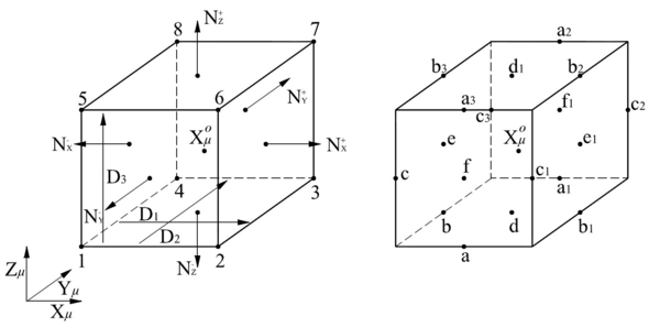
|
| Figure 71: Master and slaves nodes in a general hexagonal RVE. |
| Master nodes | a | b | c | d | e | f |
| Slave nodes | a1, a2, a3 | b1, b2, b3 | c1, c2, c3 | d1 | e1 | f1 |
| Nodes | 1 | 2 | 3 | 4 | 5 | 6 | 7 | 8 |
Considering a generic master node “a” on the axis X and its slave nodes ``, `` and `` the position vector difference between their in the reference configuration is
|
|
(B.1) |
Following the same procedure is possible to obtain the position vector difference for the other master and slave nodes as
|
|
And, for the vertices nodes are
|
|
where , and are the X, Y and Z direction size of the RVE.
B.1.1 Master-slave kinematic relationships
In the following sections the kinematic master-slave relationships will be obtained for the first-order and enhanced-first-order homogenization approaches.
B.1.1.1 First-order approach
Taking into account that Periodic boundary fluctuations condition are considered in the microscopic BVP and the proposed displacement field given by 9.9 is possible to write the displacement of the slave node `` as a function of the displacement of the master node “a” as
|
|
(B.2) |
and using the above expression
|
|
(B.3) |
To simplify the final expressions is defined: . Therefore, it can be shown that
|
|
(B.4) |
And, for the vertices nodes
|
|
(B.5) |
B.1.1.2 Enhanced first-order approach
Considering again that Periodic boundary fluctuations condition are considered in the microscopic BVP and the proposed displacement field given by 9.36, it is possible to rewrite the displacement of the slave node `` as a function of the displacement of the master node “a” for the enriched approach as
|
|
(B.6) |
using B.1, last expression can be rewritten as
|
|
(B.7) |
To simplify the final expressions is defined
|
|
Therefore, it can be shown that the slaves nodes are
|
|
(B.8) |
And, taking into account that the position vector of the master vertex node “1” is: , the slaves vertices nodes are
|
|
(B.9) |
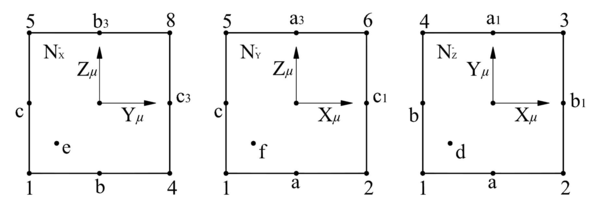
|
| Figure 72: Master and slaves nodes on the negative faces of the RVE. |
For the enhanced-first-order approach an extra boundary restrictions must be satisfied. In the Periodic boundary fluctuations considered these extra boundary conditions are integral boundary constraints on each negative face of the RVE. The extra boundary constraints described in Section 9.5.2 can be rewritten as
|
|
(B.10) |
where,
|
|
and,
|
|
Here, , and are the shape functions on the negative face , and of the RVE, respectively. And, from Figure 72 it is possible to write the displacement vectors of the nodes on the different negative faces as
|
|
In the previous displacement vectors of the nodes on the negative faces of the RVE it is possible identify masters and slaves nodes. Therefore, using B.8 and B.9 the boundary constraints B.10 above obtained can be written in terms of master nodes only as
|
|
(B.11) |
where,
|
|
and, as an example, the term of the matrix for the of the master nodes on the negative face is
|
|
and the contribution to for the of the slave nodes on the negative face is
|
|
The master nodes on the different negative faces of the RVE must verify B.11. Therefore, with the aim to find redundant unknowns, it is possible to identify another slave extra node by each negative face which can be obtained as a function of the other master nodes. Then,
|
|
(B.12) |
B.2 Elimination of the slave degrees of freedom
In the present section the reduction of the degrees of freedom on the equation system is shown for the different cases.
B.2.1 Linear implementation
Introducing the concept of master nodes and slave nodes into the equation system, it can be rewritten as
|
|
(B.13) |
where the subscripts , , and refer to the degrees of freedom of the internal nodes, master nodes and slave nodes, respectively. If the contribution of each type of degree of freedom is separated
|
|
(B.14) |
Considering that Periodic boundary fluctuations condition are taken in the microscopic problem, it is possible to write in matrix form the master-slave kinematic relationship presented in the Section B.1.1 of the Appendix B.1 as
|
|
(B.15) |
Introducing B.15 in B.14, the following expression is obtained
|
|
(B.16) |
and, it is possible to arrange the above equation as
|
|
(B.17) |
Thanks to the boundary conditions considered for the problem, it can be shown that the relationships of the displacement fluctuation field between the boundary master and slave nodes, written in a matrix form are
|
|
(B.18) |
therefore, it is possible to reduce the system of equations shown in B.17 as
|
|
(B.19) |
Defining the reduced stiffness matrix, the reduced displacements vector, and the Right-Hand Side (RHS) vector as
|
|
(B.20) |
|
|
(B.21) |
|
|
(B.22) |
therefore, the starting problem has been reduced to
|
|
(B.23) |
And finally, the reduced equation system to be solved is
|
|
(B.24) |
Equation B.24 shows that the degrees of freedom of the slave nodes are not included in the reduced displacements vector. The reduced equation system has less degrees of freedom than the original one and it also satisfies automatically the boundary conditions considered.
B.2.2 Non-linear implementation
Introducing the concept of master nodes and slave nodes into the equation system, it can be rewritten as
|
|
(B.25) |
where the subscripts , , and refer to the degrees of freedom of the internal nodes, master nodes and slave nodes, respectively. Considering the update formula of the Newton-Raphson method for the master degrees of freedom as
|
|
(B.26) |
It is possible to write B.15 in the current micro problem iteration as
|
|
(B.27) |
where the superscript is associated to the current iteration of the macro problem. Then, using B.26 the above expression can be written as
|
|
(B.28) |
and the following relationships is found
|
|
(B.29) |
|
|
(B.30) |
Considering B.18 in the above expression, it is possible to reduce the system of equations shown in B.25 as
|
|
(B.31) |
or in its reduced form using the definitions of the previous section
|
|
(B.32) |
Therefore, the reduced equation system to be solved is
|
|
(B.33) |
Equation B.33 shows that the degrees of freedom of the slave nodes are not included in the displacements vector, even for the non-linear case, and the reduced equation system also satisfies automatically the boundary conditions.
B.3 Derivatives of the shape functions
The finite element method uses the shape functions to approximate the continuous displacement field within the finite element domain. In general, the shape functions are defined in an iso-parametric domain, then
|
|
(B.34) |
The derivatives of the shape functions are computed in the iso-parametric domain as
|
|
(B.35) |
Considering that the finite element domain is approximated as
|
|
(B.36) |
where are the coordinate values of the finite element nodes in the element domain. Then, the Jacobian matrix which transforms the iso-parametric domain to the finite element domain, is defined as
|
|
(B.37) |
and
|
|
(B.38) |
The shape functions and their derivatives have to be calculated in the finite element domain
|
|
(B.39) |
Therefore, the values on the finite element domain are obtained as following:
B.3.1 Value of the shape functions
|
|
(B.40) |
B.3.2 First derivative of the shape functions
|
|
(B.41) |
B.3.3 Second derivative of the shape functions
|
|
(B.42) |
and considering the above expression
|
|
(B.43) |
Taking intro account that
|
|
(B.44) |
and
|
|
(B.45) |
It is possible to obtain the unknown term as
|
|
(B.46) |
Therefore,
|
|
(B.47) |
B.4 Derivation of displacement field, deformation gradient and gradient of the deformation gradient tensor
B.4.1 Displacement field
Taking into account the consideration made in Section B.3, the displacement field in the finite element domain can be approximated as
|
|
(B.48) |
where are the nodal displacement values of the finite element.
B.4.2 Deformation gradient tensor
If the current configuration position of the structure is approximated as
|
|
(B.49) |
where the deformation gradient tensor is obtained
|
|
(B.50) |
then,
|
|
(B.51) |
B.4.3 Gradient of the deformation gradient tensor
|
|
(B.52) |
finally,
|
|
(B.53) |
B.5 FEM implementation in PLCd code
The numerical implementation of the homogenization method is carried out through of a coupled solution scheme in two scales by means of PLCd program. The PLCd code is an implicit FEM code developed in FORTRAN by Prof. Oller's group at CIMNE [9]. The program solves solid mechanics problems which can either be linear or non-linear and take into account small or large deformation hypothesis. It has been developed to treat a large variety of composite materials through the use of different composite theories and can support materials with general anisotropy.
The basic problem in a general non-linear analysis is to find the state equilibrium of a body in function of the applied loads, by using an incremental solution approach. In the case of a static or quasi-static analysis, in which the time effect does not affect the equilibrium equations, the time factor is only a convenient variable which denote different intensities of applied load. In a classical FEM implementation the non-linear response is effectively carried out using a step-by-step incremental solution, in which the total applied load is divided into several number of load steps. Then, in each load step an iterative process must be performed until the solution for the equilibrium equation is achieved. The iterative process is conducted with a Newton-Raphson procedure. Figure 73 shows a flow diagram of the incremental solution and the iterative method implemented in PLCd code at macroscopic scale.
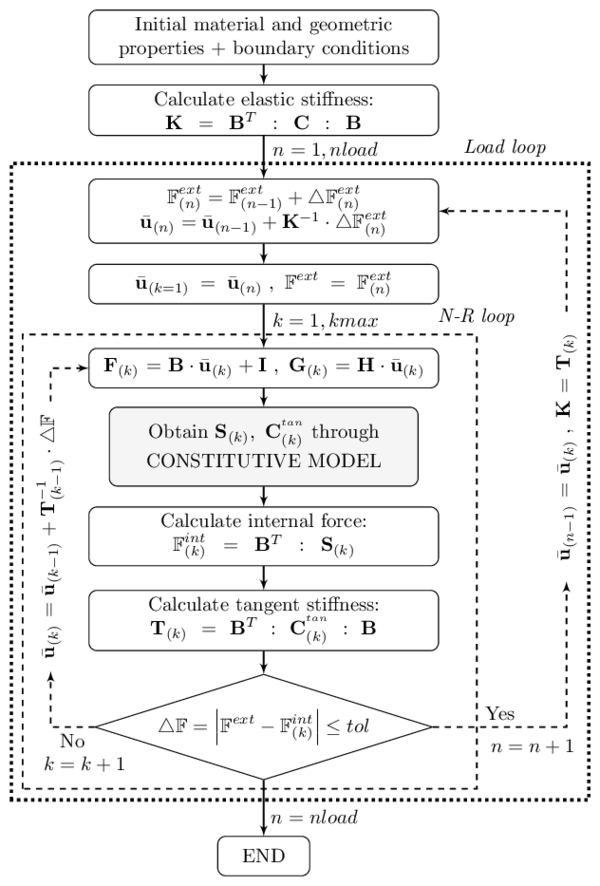
|
| Figure 73: PLCd Flow diagram of the FEM implementation at the macro-scale. |
B.5.1 PLCd FE22 implementation
In the PLCd program, the macro-scale problem is solved by a classical FE implementation and the micro-scale problem is also solved using a FE implementation. The general framework of the solution consists in solving for each Gauss point of each FE at the macro-scale, another FE problem defined by the RVE in order to address the response at the micro-scale that will give the homogenized solution of the Gauss point at the macro-scale.
However, considering that all materials in the micro-scale have an elastic behavior and assuming a perfect contact between the component materials, the elastic constitutive tensor for the composite which relates the macroscopic homogenized variables remains constant. Therefore, the expression given by 9.32 in the first-order homogenization and 9.81 in the enhanced-first-order homogenization can be expressed in a similar way as in the classical expression for homogeneous materials as
|
|
(B.54) |
where is a tensor formed by the elastic constants of the homogenized composite, called homogenized elastic constitutive tensor and and are the macroscopic or homogenized stress and strain tensors.
Rewriting B.54 using a Voigt notation , where it is possible to observe that one way to obtain this constitutive tensor of the material is by applying a macroscopic strain tensor on the RVE in order to compute the microscopic stress tensor . Then, the macroscopic stress tensor in the RVE is calculated for each macroscopic strain tensor applied according to expression given by 9.27 or 9.74.
Considering a three-dimensional problem, it is necessary six independent strains cases to obtain the homogenized constitutive tensor, each one accounting for a different principal direction. The macroscopic strain tensor for each direction is designed taking a unit value on the direction analyzed and zero for the others. For example, in the X direction case is
|
|
(B.55) |
Figure 74 shows a flow diagram with the implementation in PLCd code to calculate the homogenized constitutive tensor.
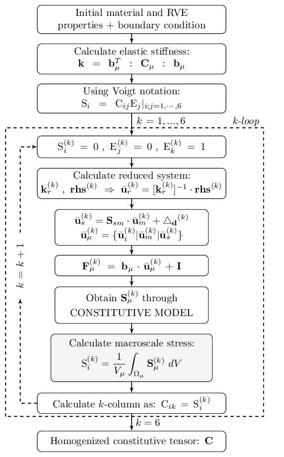
|
| Figure 74: Flow diagram of the homogenized elastic constitutive tensor calculation in PLCd code. |
B.5.1.1 Non-linear FE2 implementation
When a non-linear analysis is addressed by a FE2 numerical homogenization the non-linear response of the homogenized composite is obtained through the analysis of the RVE. Therefore, the macroscopic stress tensor is obtained through the solution of one RVE for each Gauss point at the macro-scale FE mesh. In Figure 75 is possible to observe a flow diagram of the FE2 numerical implementation developed for the FEM code used. The micro-scale problem is solved using another FE problem. Therefore, when the non-linear behavior begins on a component material in the RVE it is necessary an iterative process to address the solution. Figure 76 shows the flow diagram of the FE implementation at the micro-scale. The flow diagrams shown that for each non-linear macro-scale step there are one macro-scale iterative process and several micro-scale iterative processes for each non-linear RVE.
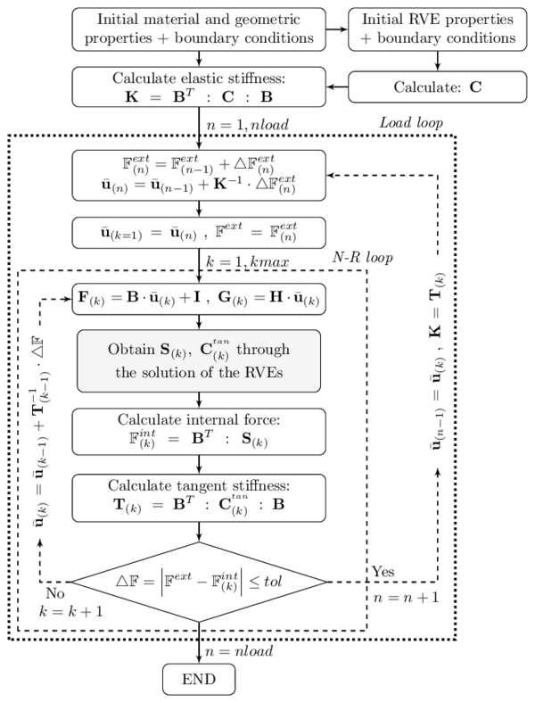
|
| Figure 75: PLCd flow diagram of the FE2 implementation. |
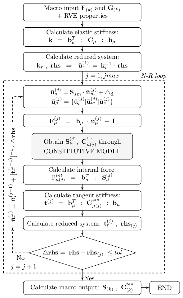
|
| Figure 76: PLCd flow diagram of the FE2 implementation at the micro-scale. |
B.5.2 Numerical tangent constitutive tensor
The perturbation method used to obtain the homogenized tangent tensor of the RVE is described in this section. It follows the same procedure defined in [33]. The tangent constitutive tensor () is defined as
|
|
(B.56) |
The matrix description given by B.56 can be written for orthotropic materials as
|
|
(B.57) |
The stress vector rate can be obtained as the sum of stress vectors, which are the product of the component of the strain vector rate and the column of the tangent tensor. Then
|
|
(B.58) |
where
|
|
(B.59) |
Equation B.58 can be used to obtain the column of the tangent constitutive tensor as
|
|
(B.60) |
The perturbation method consists in defining small variations, or perturbations, of the strain vector , to obtain stress vectors to obtain the numerical approach given by B.60 of the tangent constitutive tensor. Figure 77 is showing a flow diagram of the implementation in the PLCd of the perturbation method described to obtain the macroscopic tangent constitutive tensor.
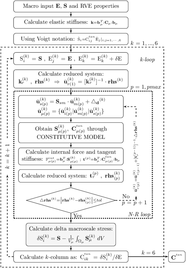
|
| Figure 77: Flow diagram of the perturbation method implemented at PLCd to obtain the macroscopic tangent constitutive tensor. |
B.5.3 PLCd parallelization and memory improvements
B.5.3.1 Parallelization tasks
The objective of parallelizing the code is to reduce the computing time in order to improve the overall performance of the FE2 homogenization method developed. The parallelization of the FEM code has been done using OpenMP (http://www.OpenMP.org).
OpenMP is a shared memory application program interface that can be implemented on a broad range of architectures. It consists in a set of compiler directives, run-time library routines and environment variables that can be added to sequential FORTRAN code in order to specify how the work is to be accessed and shared among threads that will execute on different processors or cores and to order accesses to the shared data as needed.
According to Amdahl's law, to obtain a maximum speedup or scalability, in a parallel program, is important parallelize the maximum percentage of the code. Therefore, the parallelization of a computational code is an unfinished task. Because of this, during the study many sequential loops in the PLCd have been parallelized to improve the scalability, such as convergence element loop, writing database no-converged to converged element loop, assemble sparse stiffness matrix element loop and assemble residual forces vector element loop.
On the other hand, in a non-linear analysis, the tasks balance between the cores is a significant variable to maintain the speedup. Then, an efficient parallelization strategy in the constitutive element loop (see Figure 78) has been addressed with the aim to improve the tasks balance in the threads during a non-linear analysis. The ``OMP_SET_SCHEDULE(type,chunk) instruction is used to configure the parallel strategy. In the default static type strategy the number of elements is divided into the number of threads and they are assigned to the threads at the beginning of the loop. Therefore, when a thread receives many elements with a non-linear behavior the tasks balance is lost. This situation is more critical in a FE2 implementation because the composite constitutive model is another micro FE problem. To conserve a good tasks balance a dynamic type strategy with a chunk of 1 is set. The dynamic strategy assigns the chunk quantity of elements to the threads at the beginning and then, when a thread has finished with that task, a new chunk number of elements is assigned to it. In other works, the tasks assigned to each thread is dynamic.
B.5.3.2 Memory manager
The advantage of the reduced memory requirement of the multiscale approach in linear range is lost when the method is extended to non-linear case. The non-linear behavior of the component materials in the RVE depend of the internal variables and strain tensor history. Therefore, the internal RVE database for each Gauss point of the macro-scale mesh should be saved in the memory. To minimize the memory requirements for non-linear analyses a management procedure to assign dynamic memory is implemented in PLCd code. While all component materials in the RVE of the macro Gauss point are in the elastic range the code does not reserve memory for the internal RVE database. However, if some micro Gauss points of the RVE of a macro Gauss point begin with a non-linear behavior only for these Gauss points is reserved space in memory. With this memory strategy, the memory requirement for non-linear analyses through a multiscale homogenization is reduced to the minimum required.
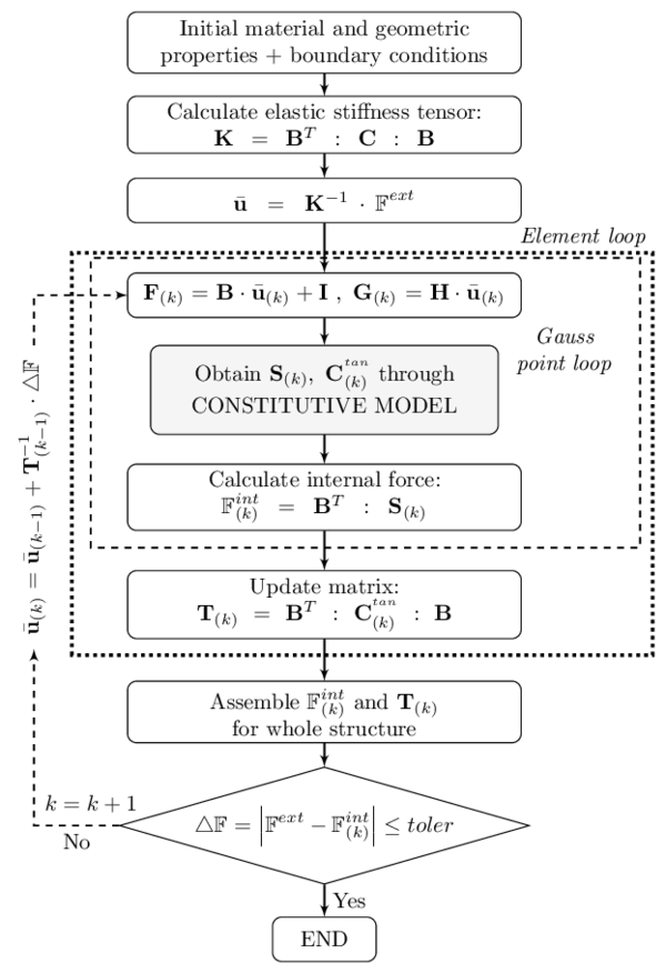
|
| Figure 78: PLCd flow diagram of the parallel element loop implementation at the macro-scale. |
References
[1] Zienkiewicz, O.C. and Taylor, R.L. and Zhu, J.Z. (2013) "The Finite Element Method: Its Basis and Fundamentals". Elsevier Ltd, Seventh Edition
[2] Truesdell, C. and Toupin, R. (1960) "The Classical Field Theories", Volume 3. Springer-Verlag 226–858
[3] Oller, Sergio. (2014) "Numerical Simulation of Mechanical Behavior of Composite Materials". Springer International Publishing
[4] Rastellini, Fernando and Oller, Sergio and Salomón, Omar and Oñate, Eugenio. (2008) "Composite materials non-linear modelling for long fibre-reinforced laminates. Continuum basis, computational aspects and validations", Volume 86. Computers and Structures 9 879–896
[5] Hill, R. (1963) "Elastic properties of reinforced solids: Some theoretical principles", Volume 11. Journal of the Mechanics and Physics of Solids 5 357–372
[6] Suquet, Pierre M. (1985) "Local and global aspects in the mathematical theory of plasticity". Plasticity Today - Modeling Methods and Applications. Elsevier, London 279–310
[7] Smit, R.J.M. and Brekelmans, W.A.M. and Meijer, H.E.H. (1998) "Prediction of the mechanical behavior of nonlinear heterogeneous systems by multi-level finite element modeling", Volume 155. Computer Methods in Applied Mechanics and Engineering 1-2 181–192
[8] Kouznetsova, V. G. and Geers, M. G. D. and Brekelmans, W. A. M. (2004) "Multi-scale second-order computational homogenization of multi-phase materials: a nested finite element solution strategy", Volume 193. Computer Methods in Applied Mechanics and Engineering 48-51 5525–5550
[9] PLCd research group "PLCd: Non-linear thermo-mechanic finite element code for research-oriented applications". Free access code developed at CIMNE. Available from: http://www.cimne.com/PLCd, 1991-to present
[10] Melendo, A and Coll, A and Pasenau, M and Escolano, E and Monros, A. (2015) "www.gidhome.com"
[11] Coll, A and Ribó, R and Pasenau, M and Escolano, E and Perez, J.Suit. and Melendo, A and Monros, A. (2014) "GiD v.12 Customization Manual". CIMNE
[12] Barbero, Ever J. (2010) "Introduction to composite materials design". CRC Press, Second Edition
[13] Jayatilaka, Ayal de S. (1979) "Fracture of engineering brittle materials". Elsevier Science Ltd 378
[14] Halpin Affdl, J. C. and Kardos, J L. (1976) "The Halpin-Tsai equations: A review", Volume 16. Polymer Engineering and Science 5 344–352
[15] Neamtu, L and Oller, S and Oñate, E. (1997) "A generalized mixing theory elasto-damage-plastic model for finite element analysis of composites". Computational plasticity 1214–1219
[16] Oller, S. and Oñate, E. and Miquel, J. and Botello, S. (1996) "A plastic damage constitutive model for composite materials", Volume 33. International Journal of Solids and Structures 17 2501–2518
[17] Truesdell, C. (1962) "Mechanical Basis of Diffusion", Volume 37. The Journal of Chemical Physics 10 2336
[18] Green, A. E. and Adkins, J. E. (1964) "A contribution to the theory of non-linear diffusion", Volume 15. Archive for Rational Mechanics and Analysis 3 235–246
[19] Ortiz, M and Popov, E. P. (1982) "A Physical Model for the Inelasticity of Concrete", Volume 383. Proceedings of the Royal Society A: Mathematical, Physical and Engineering Sciences 1784 101–125
[20] Ortiz, Miguel and Popov, Egor P. (1982) "Plain concrete as a composite material", Volume 1. Mechanics of Materials 2 139–150
[21] Oller, S. (1988) "Un modelo constitutivo de daño continuo para materiales friccionales". Department of strength of materials and structures in engineering. Technical University of Catalonia
[22] Lubliner, J. and Oliver, J. and Oller, S. and Oñate, E. (1989) "A plastic-damage model for concrete", Volume 25. International Journal of Solids and Structures 3 299–326
[23] Lubliner, Jacob. (1990) "Plasticity theory". Collier Macmillan
[24] Oller, S. and Oñate, E. (1996) "A hygro-thermo-mechanical constitutive model for multiphase composite materials", Volume 33. International Journal of Solids and Structures 20-22 3179–3186
[25] Oller, S and Neamtu, L and Oñate, E. (1995) "Una generalización de la teoría de mezclas clásica para el tratamiento de compuestos en serie/paralelo". Congreso Nacional de Materiales Compuestos 433–438
[26] Car, E. and Oller, S. and Oñate, E. (2000) "An anisotropic elastoplastic constitutive model for large strain analysis of fiber reinforced composite materials", Volume 185. Computer Methods in Applied Mechanics and Engineering 2-4 245–277
[27] Mata, P. and Oller, S. and Barbat, A.H. (2007) "Static analysis of beam structures under nonlinear geometric and constitutive behavior", Volume 196. Computer Methods in Applied Mechanics and Engineering 45-48 4458–4478
[28] Martínez, Xavier and Oller, Sergio and Barbero, Ever. (2008) "Study of Delamination in Composites by Using the Serial/Parallel Mixing Theory and a Damage Formulation". Mechanical Response of Composites. Springer Netherlands 119–140
[29] Martinez, Xavier and Oller, Sergio. (2009) "Numerical Simulation of Matrix Reinforced Composite Materials Subjected to Compression Loads", Volume 16. Archives of Computational Methods in Engineering 4 357–397
[30] Paredes, Jairo A. and Barbat, Alex H. and Oller, Sergio. (2011) "A compression–tension concrete damage model, applied to a wind turbine reinforced concrete tower", Volume 33. Engineering Structures 12 3559–3569
[31] Martinez, Xavier and Rastellini, Fernando and Oller, Sergio and Flores, Fernando and Oñate, Eugenio. (2011) "Computationally optimized formulation for the simulation of composite materials and delamination failures", Volume 42. Composites Part B: Engineering 2 134–144
[32] Pérez, Marco A. and Martínez, Xavier and Oller, Sergio and Gil, Lluís and Rastellini, Fernando and Flores, Fernando. (2013) "Impact damage prediction in carbon fiber-reinforced laminated composite using the matrix-reinforced mixing theory", Volume 104. Composite Structures 239–248
[33] Martinez, Xavier and Oller, Sergio and Rastellini, Fernando and Barbat, Alex H. (2008) "A numerical procedure simulating RC structures reinforced with FRP using the serial/parallel mixing theory", Volume 86. Computers and Structures 15-16 1604–1618
[34] Iijima, Sumio. (1991) "Helical microtubules of graphitic carbon", Volume 354. Nature 6348 56–58
[35] Coleman, Jonathan N. and Khan, Umar and Blau, Werner J. and Gun’ko, Yurii K. (2006) "Small but strong: A review of the mechanical properties of carbon nanotube–polymer composites", Volume 44. Carbon 9 1624–1652
[36] Ruoff, Rodney S. and Lorents, Donald C. (1995) "Mechanical and thermal properties of carbon nanotubes", Volume 33. Carbon 7 925–930
[37] Salvetat, J-P and Bonard, J-M and Thomson, N.H. and Kulik, A.J. and Forró, L. and Benoit, W and Zuppiroli, L. (1999) "Mechanical properties of carbon nanotubes", Volume 69. Applied Physics A: Materials Science and Processing 3 255–260
[38] Cadek, M and Murphy, R and McCarthy, B and Drury, A and Lahr, B and Barklie, R.C and in het Panhuis, M and Coleman, J.N and Blau, W.J. (2002) "Optimisation of the arc-discharge production of multi-walled carbon nanotubes", Volume 40. Carbon 6 923–928
[39] Yu, Min-Feng and Lourie, Oleg and Dyer, Mark J. and Moloni, Katerina and Kelly, Thomas F. and Ruoff, Rodney S. (2000) "Strength and Breaking Mechanism of Multiwalled Carbon Nanotubes Under Tensile Load", Volume 287. Science 5453 637–640
[40] Salvetat, Jean-Paul and Kulik, Andrzej J and Bonard, Jean-Marc and Briggs, G Andrew D and Stöckli, Thomas and Méténier, Karine and Bonnamy, Sylvie and Béguin, Francois and Burnham, Nancy A and Forró, Lásló. (1999) "Elastic Modulus of Ordered and Disordered Multiwalled Carbon Nanotubes", Volume 11. Advanced Materials 2 161–165
[41] Xie, Sishen and Li, Wenzhi and Pan, Zhengwei and Chang, Baohe and Sun, Lianfeng. (2000) "Mechanical and physical properties on carbon nanotube", Volume 61. Journal of Physics and Chemistry of Solids 7 1153–1158
[42] Cadek, M and Coleman, J N and Ryan, K P and Nicolosi, V and Bister, G and Fonseca, A and Nagy, J B and Szostak, K and Béguin, F and Blau, W J. (2004) "Reinforcement of Polymers with Carbon Nanotubes: The Role of Nanotube Surface Area", Volume 4. Nano Letters 2 353–356
[43] McCarthy, B and Coleman, J N and Czerw, R and Dalton, A B and in het Panhuis, M and Maiti, A and Drury, A and Bernier, P and Nagy, J B and Lahr, B and Byrne, H J and Carroll, D L and Blau, W J. (2002) "A Microscopic and Spectroscopic Study of Interactions between Carbon Nanotubes and a Conjugated Polymer", Volume 106. The Journal of Physical Chemistry B 9 2210–2216
[44] McCarthy, B and Coleman, J N and Curran, S A and Dalton, A B and Davey, A P and Konya, Z and Fonseca, A and Nagy, J B and Blau, W J. (2000) "Observation of site selective binding in a polymer nanotube composite", Volume 19. Journal of Materials Science Letters 24 2239–2241
[45] Yang, Mingjun and Koutsos, Vasileios and Zaiser, Michael. (2005) "Interactions between Polymers and Carbon Nanotubes: A Molecular Dynamics Study", Volume 109. The Journal of Physical Chemistry B 20 10009–10014
[46] Tsuda, Terumasa and Ogasawara, Toshio and Deng, Fei and Takeda, Nobuo. (2011) "Direct measurements of interfacial shear strength of multi-walled carbon nanotube/PEEK composite using a nano-pullout method", Volume 71. Composites Science and Technology 10 1295–1300
[47] Cooper, Carole A. and Cohen, Sidney R. and Barber, Asa H. and Wagner, H. Daniel. (2002) "Detachment of nanotubes from a polymer matrix", Volume 81. Applied Physics Letters 20 3873
[48] Barber, Asa H. and Cohen, Sidney R. and Wagner, H. Daniel. (2003) "Measurement of carbon nanotube–polymer interfacial strength", Volume 82. Applied Physics Letters 23 4140
[49] Ding, W and Eitan, A and Fisher, F T and Chen, X and Dikin, D A and Andrews, R and Brinson, L C and Schadler, L S and Ruoff, R S. (2003) "Direct Observation of Polymer Sheathing in Carbon Nanotube-Polycarbonate Composites", Volume 3. Nano Letters 11 1593–1597
[50] Sandler, Jan and Werner, Philipp and Shaffer, Milo S.P and Demchuk, Vitaly and Altstädt, Volker and Windle, Alan H. (2002) "Carbon-nanofibre-reinforced poly(ether ether ketone) composites", Volume 33. Composites Part A: Applied Science and Manufacturing 8 1033–1039
[51] Sandler, J and Broza, G and Nolte, M and Schulte, K and Lam, Y. -M. and Shaffer, M S P. (2003) "Crystallization of Carbon Nanotube and Nanofiber Polypropylene Composites", Volume 42. Journal of Macromolecular Science, Part B 3 479–488
[52] Wagner, H D and Lourie, O and Feldman, Y and Tenne, R. (1998) "Stress-induced fragmentation of multiwall carbon nanotubes in a polymer matrix", Volume 72. Applied Physics Letters 2 188
[53] Frankland, S J V and Caglar, A and Brenner, D W and Griebel, M. (2002) "Molecular simulation of the influence of chemical cross-links on the shear strength of carbon nanotube-polymer interfaces", Volume 106. The Journal of Physical Chemistry B 12 3046–3048
[54] Garg, Ajay and Sinnott, Susan B. (1998) "Effect of chemical functionalization on the mechanical properties of carbon nanotubes", Volume 295. Chemical Physics Letters 4 273–278
[55] Liao, Kin and Li, Sean. (2001) "Interfacial characteristics of a carbon nanotube–polystyrene composite system", Volume 79. Applied Physics Letters 25 4225
[56] Lordi, Vincenzo and Yao, Nan. (2000) "Molecular mechanics of binding in carbon-nanotube–polymer composites", Volume 15. Journal of Materials Research 12 2770–2779
[57] Barber, Asa H. and Cohen, Sidney R. and Kenig, Shmuel and Wagner, H.Daniel. (2004) "Interfacial fracture energy measurements for multi-walled carbon nanotubes pulled from a polymer matrix", Volume 64. Composites Science and Technology 15 2283–2289
[58] Hwang, G. L. and Shieh, Y-T and Hwang, K. C. (2004) "Efficient Load Transfer to Polymer-Grafted Multiwalled Carbon Nanotubes in Polymer Composites", Volume 14. Advanced Functional Materials 5 487–491
[59] Xia, Hesheng and Wang, Qi and Qiu, Guihua. (2003) "Polymer-Encapsulated Carbon Nanotubes Prepared through Ultrasonically Initiated In Situ Emulsion Polymerization", Volume 15. Chemistry of Materials 20 3879–3886
[60] Lou, Xudong and Detrembleur, Christophe and Sciannamea, Valérie and Pagnoulle, Christophe and Jérome, Robert. (2004) "Grafting of alkoxyamine end-capped (co)polymers onto multi-walled carbon nanotubes", Volume 45. Polymer 18 6097–6102
[61] Bhattacharyya, S. and Sinturel, C. and Salvetat, J. P. and Saboungi, M.-L. (2005) "Protein-functionalized carbon nanotube-polymer composites", Volume 86. Applied Physics Letters 11 113104
[62] Deng, Fei and Ogasawara, Toshio and Takeda, Nobuo. (2007) "Tensile properties at different temperature and observation of micro deformation of carbon nanotubes–poly(ether ether ketone) composites", Volume 67. Composites Science and Technology 14 2959–2964
[63] F. Otero and X. Martinez and S. Oller and O. Salomon. (2012) "Study and prediction of the mechanical performance of a nanotube-reinforced composite", Volume 94. Composite Structures 9 2920 - 2930
[64] A.R. Melro and P.P. Camanho and F.M. Andrade Pires and S.T. Pinho. (2013) "Micromechanical analysis of polymer composites reinforced by unidirectional fibres: Part l – Constitutive modelling", Volume 50. International Journal of Solids and Structures 11–12 1897 - 1905
[65] Coleman, Jonathan N. and Cadek, Martin and Ryan, Kevin P. and Fonseca, Antonio and Nagy, Janos B. and Blau, Werner J. and Ferreira, Mauro S. (2006) "Reinforcement of polymers with carbon nanotubes. The role of an ordered polymer interfacial region. Experiment and modeling", Volume 47. Polymer 26 8556–8561
[66] Cadek, M. and Coleman, J. N. and Barron, V. and Hedicke, K. and Blau, W. J. (2002) "Morphological and mechanical properties of carbon-nanotube-reinforced semicrystalline and amorphous polymer composites", Volume 81. Applied Physics Letters 27 5123
[67] Malvern, L E. (1969) "Introduction to the mechanics of a continuous medium". Prentice Hall
[68] Thostenson, E T and Chou, T. (2003) "On the elastic properties of carbon nanotube-based composites: modelling and characterization", Volume 36. Journal of Physics D: Applied Physics 5 573–582
[69] Zhou, X. and Shin, Eungsoo and Wang, K.W. and Bakis, C.E. (2004) "Interfacial damping characteristics of carbon nanotube-based composites", Volume 64. Composites Science and Technology 15 2425–2437
[70] Coleman, J. N. and Cadek, M and Blake, R and Nicolosi, V and Ryan, K. P. and Belton, C and Fonseca, A and Nagy, J. B. and Gun'ko, Y. K. and Blau, W. J. (2004) "High Performance Nanotube-Reinforced Plastics: Understanding the Mechanism of Strength Increase", Volume 14. Advanced Functional Materials 8 791–798
[71] Cox, H L. (1952) "The elasticity and strength of paper and other fibrous materials", Volume 3. British Journal of Applied Physics 3 72–79
[72] Krenchel, Herbert. (1964) "Fibre reinforcement : theoretical and practical investigations of the elasticity and strength of fibre-reinforced materials". Copenhagen : Akademisk Forlag
[73] Meng, H. and Sui, G.X. and Fang, P.F. and Yang, R. (2008) "Effects of acid- and diamine-modified MWNTs on the mechanical properties and crystallization behavior of polyamide 6", Volume 49. Polymer 2 610–620
[74] Li, Chunyu and Chou, TW. (2003) "Elastic moduli of multi-walled carbon nanotubes and the effect of van der Waals forces", Volume 63. Composites Science and Technology 11 1517–1524
[75] Maurin, Romain and Davies, Peter and Baral, Nicolas and Baley, Christophe. (2008) "Transverse Properties of Carbon Fibres by Nano-Indentation and Micro-mechanics", Volume 15. Applied Composite Materials 2 61–73
[76] Díez-Pascual, Ana M. and Naffakh, Mohammed and González-Domínguez, José M. and Ansón, Alejandro and Martínez-Rubi, Yadienka and Martínez, M. Teresa and Simard, Benoit and Gómez, Marián A. (2010) "High performance PEEK/carbon nanotube composites compatibilized with polysulfones-I. Structure and thermal properties", Volume 48. Carbon 12 3485–3499
[77] Díez-Pascual, Ana M. and Naffakh, Mohammed and González-Domínguez, José M. and Ansón, Alejandro and Martínez-Rubi, Yadienka and Martínez, M. Teresa and Simard, Benoit and Gómez, Marián A. (2010) "High performance PEEK/carbon nanotube composites compatibilized with polysulfones-II. Mechanical and electrical properties", Volume 48. Carbon 12 3500–3511
[78] Jiang, Zhenyu and Hornsby, Peter and McCool, Rauri and Murphy, Adrian. (2012) "Mechanical and thermal properties of polyphenylene sulfide/multiwalled carbon nanotube composites", Volume 123. Journal of Applied Polymer Science 5 2676–2683
[79] Koratkar, Nikhil A. and Suhr, Jonghwan and Joshi, Amit and Kane, Ravi S. and Schadler, Linda S. and Ajayan, Pulickel M. and Bartolucci, Steve. (2005) "Characterizing energy dissipation in single-walled carbon nanotube polycarbonate composites", Volume 87. Applied Physics Letters 6 063102
[80] Gibson, Ronald F. and Ayorinde, Emmanuel O. and Wen, Yuan-Feng. (2007) "Vibrations of carbon nanotubes and their composites: A review", Volume 67. Composites Science and Technology 1 1–28
[81] Eshelby, J D. (1957) "The Determination of the Elastic Field of an Ellipsoidal Inclusion, and Related Problems", Volume 241. Proceedings of the Royal Society A: Mathematical, Physical and Engineering Sciences 1226 376–396
[82] Hill, R. (1965) "A self-consistent mechanics of composite materials", Volume 13. Journal of the Mechanics and Physics of Solids 4 213–222
[83] Hashin, Z. and Shtrikman, S. (1962) "On some variational principles in anisotropic and nonhomogeneous elasticity", Volume 10. Journal of the Mechanics and Physics of Solids 4 335–342
[84] Ponte Castañeda, P. (1992) "New variational principles in plasticity and their application to composite materials", Volume 40. Journal of the Mechanics and Physics of Solids 8 1757–1788
[85] Bensoussan, A. and Lions, J.L. and Papanicolaou, G. (1978) "Asymptotic Analysis for Periodic Structures". North-Holland
[86] Sanchez-Palencia, E. (1980) "Non-Homogeneous Media and Vibration Theory", Volume 127. Lecture Notes in Physics. Springer-Verlag
[87] Hashin, Zvi. (1962) "The Elastic Moduli of Heterogeneous Materials", Volume 29. Journal of Applied Mechanics 1 143–150
[88] Mori, T and Tanaka, K. (1973) "Average stress in matrix and average elastic energy of materials with misfitting inclusions", Volume 21. Acta Metallurgica 5 571–574
[89] Christensen, R.M. and Lo, K.H. (1979) "Solutions for effective shear properties in three phase sphere and cylinder models", Volume 27. Journal of the Mechanics and Physics of Solids 4 315–330
[90] Mercier, S. and Molinari, A. (2009) "Homogenization of elastic–viscoplastic heterogeneous materials: Self-consistent and Mori-Tanaka schemes", Volume 25. International Journal of Plasticity 6 1024–1048
[91] Molinari, Alain. (2002) "Averaging Models for Heterogeneous Viscoplastic and Elastic Viscoplastic Materials", Volume 124. Journal of Engineering Materials and Technology 1 62
[92] Mercier, S and Jacques, N and Molinari, A. (2005) "Validation of an interaction law for the Eshelby inclusion problem in elasto-viscoplasticity", Volume 42. International Journal of Solids and Structures 7 1923–1941
[93] Walpole, L.J. (1966) "On bounds for the overall elastic moduli of inhomogeneous systems—I", Volume 14. Journal of the Mechanics and Physics of Solids 3 151–162
[94] Walpole, L.J. (1966) "On bounds for the overall elastic moduli of inhomogeneous systems—II", Volume 14. Journal of the Mechanics and Physics of Solids 5 289–301
[95] Lahellec, Noël and Suquet, Pierre. (2007) "On the effective behavior of nonlinear inelastic composites: I. Incremental variational principles", Volume 55. Journal of the Mechanics and Physics of Solids 9 1932–1963
[96] Lahellec, Noël and Suquet, Pierre. (2007) "On the effective behavior of nonlinear inelastic composites: II A second-order procedure", Volume 55. Journal of the Mechanics and Physics of Solids 9 1964–1992
[97] Sanchez-Palencia, E. (1983) "Homogenization method for the study of composite media", Volume 985. Asymptotic Analysis II —. Springer Berlin Heidelberg 192–214
[98] Fish, Jacob and Yu, Qing and Shek, Kamlun. (1999) "Computational damage mechanics for composite materials based on mathematical homogenization", Volume 45. International Journal for Numerical Methods in Engineering 11 1657–1679
[99] Gitman, I.M. and Askes, H. and Sluys, L.J. (2007) "Representative volume: Existence and size determination", Volume 74. Engineering Fracture Mechanics 16 2518–2534
[100] Ostoja-Starzewski, M. (2002) "Microstructural Randomness Versus Representative Volume Element in Thermomechanics", Volume 69. Journal of Applied Mechanics 1 25–35
[101] Terada, Kenjiro and Hori, Muneo and Kyoya, Takashi and Kikuchi, Noboru. (2000) "Simulation of the multi-scale convergence in computational homogenization approaches", Volume 37. International Journal of Solids and Structures 16 2285–2311
[102] Renard, J and Marmonier, M F. (1987) "Etude de linitiation de lendommagement dans la matrice dun matériau composite par une méthode dhomogénéisation", Volume 6. Aerospace Science and Technology 37–51
[103] Guedes, JoséMiranda and Kikuchi, Noboru. (1990) "Preprocessing and postprocessing for materials based on the homogenization method with adaptive finite element methods", Volume 83. Computer Methods in Applied Mechanics and Engineering 2 143–198
[104] Swan, Colby C. (1994) "Techniques for stress- and strain-controlled homogenization of inelastic periodic composites", Volume 117. Computer Methods in Applied Mechanics and Engineering 3-4 249–267
[105] Michel, J.C. and Moulinec, H. and Suquet, P. (1999) "Effective properties of composite materials with periodic microstructure: a computational approach", Volume 172. Computer Methods in Applied Mechanics and Engineering 1-4 109–143
[106] Haj-Ali, Rami M. and Muliana, Anastasia H. (2003) "A micromechanical constitutive framework for the nonlinear viscoelastic behavior of pultruded composite materials", Volume 40. International Journal of Solids and Structures 5 1037–1057
[107] Haj-Ali, Rami M. and Muliana, Anastasia H. (2004) "A multi-scale constitutive formulation for the nonlinear viscoelastic analysis of laminated composite materials and structures", Volume 41. International Journal of Solids and Structures 13 3461–3490
[108] Haj-Ali, Rami and Kilic, Hakan and Muliana, Anastasia. (2007) "Nested nonlinear micromechanical and structural models for the analysis of thick-section composite materials and structures", Volume 67. Composites Science and Technology 10 1993–2004
[109] Matsui, Kazumi and Terada, Kenjiro and Yuge, Kohei. (2004) "Two-scale finite element analysis of heterogeneous solids with periodic microstructures", Volume 82. Computers and Structures 7-8 593–606
[110] Ladeveze, Pierre and Nouy, Anthony. (2003) "On a multiscale computational strategy with time and space homogenization for structural mechanics", Volume 192. Computer Methods in Applied Mechanics and Engineering 28-30 3061–3087
[111] Ladeveze, Pierre and Néron, David and Gosselet, Pierre. (2007) "On a mixed and multiscale domain decomposition method", Volume 196. Computer Methods in Applied Mechanics and Engineering 8 1526–1540
[112] Oller, S and Miquel Canet, J. and Zalamea, F. (2005) "Composite Material Behavior Using a Homogenization Double Scale Method", Volume 131. Journal of Engineering Mechanics 1 65–79
[113] Zalamea, F. (2000) "Tratamiento numérico de materiales compuestos mediante la teoría de homogeneización (in Spanish)". Department of strength of materials and structures in engineering. Technical University of Catalonia
[114] de Souza Neto, E.A. and Feijóo, R.A. (2008) "On the equivalence between spatial and material volume averaging of stress in large strain multi-scale solid constitutive models", Volume 40. Mechanics of Materials 10 803–811
[115] Kouznetsova, V. and Geers, M. G. D. and Brekelmans, W. A. M. (2002) "Multi-scale constitutive modelling of heterogeneous materials with a gradient-enhanced computational homogenization scheme", Volume 54. International Journal for Numerical Methods in Engineering 8 1235–1260
[116] Geers, M G D and Coenen, E W C and Kouznetsova, V G. (2007) "Multi-scale computational homogenization of structured thin sheets", Volume 15. Modelling and Simulation in Materials Science and Engineering 4 S393–S404
[117] Coenen, E W C and Kouznetsova, V G and Geers, M G D. (2010) "Computational homogenization for heterogeneous thin sheets", Volume 83. International Journal for Numerical Methods in Engineering 8-9 1180–1205
[118] Miehe, Christian. (2002) "Strain-driven homogenization of inelastic microstructures and composites based on an incremental variational formulation", Volume 55. International Journal for Numerical Methods in Engineering 11 1285–1322
[119] Otero, F. and Oller, S. and Martinez, X. and Salomón, O. (2015) "Numerical homogenization for composite materials analysis. Comparison with other micro mechanical formulations", Volume 122. Composite Structures 405–416
[120] Otero, F. and Martinez, X. and Oller, S. and Salomón, O. (2015) "An efficient multi-scale method for non-linear analysis of composite structures", Volume 131. Composite Structures 707–719
[121] Kaczmarczyk, Łukasz and Pearce, Chris J. and Biani, Nenad. (2008) "Scale transition and enforcement of RVE boundary conditions in second-order computational homogenization", Volume 74. International Journal for Numerical Methods in Engineering 3 506–522
[122] Kouznetsova, V. G. (2002) "Computational homogenization for the multi-scale analysis of multi-phase materials". Eindhoven University of Technology, Eindhoven, The Netherlands
[123] Otero, Fermin and Oller, Sergio and Martinez, Xavier. (2016) "Multiscale Computational Homogenization: Review and Proposal of a New Enhanced-First-Order Method". Archives of Computational Methods in Engineering 1–27
[124] Geers, M. G. D. and Kouznetsova, V. G. and Brekelmans, W. A. M. (2010) "Multi-scale computational homogenization: Trends and challenges", Volume 234. Journal of Computational and Applied Mathematics 7 2175–2182
[125] Hill, R. (1984) "On macroscopic effects of heterogeneity in elastoplastic media at finite strain", Volume 95. Mathematical Proceedings of the Cambridge Philosophical Society 03 481
[126] Nemat-Nasser, Sia. (1999) "Averaging theorems in finite deformation plasticity", Volume 31. Mechanics of Materials 8 493–523
[127] Mandel, J. (1971) "Plasticité Classique Et Viscoplasticité". Springer-Verlag
[128] de Souza Neto, E. A. and Feijóo, R. A. (2006) "Variational foundations of multi-scale constitutive models of solid: small and large strain kinematical formulation", Volume 16. LNCC research and development report, No 16. National laboratory for scientific computing
[129] Coenen, E.W.C. and Kouznetsova, V.G. and Geers, M.G.D. (2012) "Novel boundary conditions for strain localization analyses in microstructural volume elements", Volume 90. International Journal for Numerical Methods in Engineering 1 1–21
[130] van der Sluis, O. and Schreurs, P.J.G. and Brekelmans, W.A.M. and Meijer, H.E.H. (2000) "Overall behaviour of heterogeneous elastoviscoplastic materials: effect of microstructural modelling", Volume 32. Mechanics of Materials 8 449–462
[131] Kanit, T. and Forest, S. and Galliet, I. and Mounoury, V. and Jeulin, D. (2003) "Determination of the size of the representative volume element for random composites: statistical and numerical approach", Volume 40. International Journal of Solids and Structures 13-14 3647–3679
[132] Kanit, Toufik and N’Guyen, Franck and Forest, Samuel and Jeulin, Dominique and Reed, Matt and Singleton, Scott. (2006) "Apparent and effective physical properties of heterogeneous materials: Representativity of samples of two materials from food industry", Volume 195. Computer Methods in Applied Mechanics and Engineering 33-36 3960–3982
[133] Miehe, C. and Dettmar, J. and Zäh, D. (2010) "Homogenization and two-scale simulations of granular materials for different microstructural constraints", Volume 83. International Journal for Numerical Methods in Engineering 8-9 1206–1236
[134] Peri, D. and de Souza Neto, E. A. and Feijóo, R. A. and Partovi, M. and Molina, A. J. Carneiro. (2011) "On micro-to-macro transitions for multi-scale analysis of non-linear heterogeneous materials: unified variational basis and finite element implementation", Volume 87. International Journal for Numerical Methods in Engineering 1-5 149–170
[135] Ghosh, Somnath and Bai, Jie and Paquet, Daniel. (2009) "Homogenization-based continuum plasticity-damage model for ductile failure of materials containing heterogeneities", Volume 57. Journal of the Mechanics and Physics of Solids 7 1017–1044
[136] Mahmoodi, M.J. and Aghdam, M.M. and Shakeri, M. (2010) "Micromechanical modeling of interface damage of metal matrix composites subjected to off-axis loading", Volume 31. Materials & Design 2 829–836
[137] Kim, B.R. and Lee, H.K. (2010) "Elastoplastic modeling of circular fiber-reinforced ductile matrix composites considering a finite RVE", Volume 47. International Journal of Solids and Structures 6 827–836
[138] A.R. Melro and P.P. Camanho and F.M. Andrade Pires and S.T. Pinho. (2013) "Micromechanical analysis of polymer composites reinforced by unidirectional fibres: Part ll – Micromechanical analyses", Volume 50. International Journal of Solids and Structures 11–12 1906 - 1915
[139] A. Arteiro and G. Catalanotti and A.R. Melro and P. Linde and P.P. Camanho. (2014) "Micro-mechanical analysis of the in situ effect in polymer composite laminates", Volume 116. Composite Structures 827 - 840
[140] Mesarovic, Sinisa Dj. and Padbidri, Jagan. (2005) "Minimal kinematic boundary conditions for simulations of disordered microstructures", Volume 85. Philosophical Magazine 1 65–78
[141] Inglis, Helen M. and Geubelle, Philippe H. and Matous, Karel. (2008) "Boundary condition effects on multiscale analysis of damage localization", Volume 88. Philosophical Magazine 16 2373–2397
[142] Giusti, S.M. and Blanco, P.J. and de Souza Netoo, E.A. and Feijóo, R.A. (2009) "An assessment of the Gurson yield criterion by a computational multi-scale approach", Volume 26. Engineering Computations 3 281–301
[143] Würkner, Mathias and Berger, Harald and Gabbert, Ulrich. (2014) "Numerical investigations of effective properties of fiber reinforced composites with parallelogram arrangements and imperfect interface", Volume 116. Composite Structures 388–394
[144] Pontefisso, Alessandro and Zappalorto, Michele and Quaresimin, Marino. (2015) "An efficient RVE formulation for the analysis of the elastic properties of spherical nanoparticle reinforced polymers", Volume 96. Computational Materials Science 319–326
[145] Bazant, Zdenek P. (2010) "Can Multiscale-Multiphysics Methods Predict Softening Damage and Structural Failure?", Volume 8. International Journal for Multiscale Computational Engineering 1 61–67
[146] Yvonnet, J. and He, Q.-C. (2007) "The reduced model multiscale method (R3M) for the non-linear homogenization of hyperelastic media at finite strains", Volume 223. Journal of Computational Physics 1 341–368
[147] Monteiro, E. and Yvonnet, J. and He, Q.C. (2008) "Computational homogenization for nonlinear conduction in heterogeneous materials using model reduction", Volume 42. Computational Materials Science 4 704–712
[148] Hernández, J.A. and Oliver, J. and Huespe, A.E. and Caicedo, M.A. and Cante, J.C. (2014) "High-performance model reduction techniques in computational multiscale homogenization", Volume 276. Computer Methods in Applied Mechanics and Engineering 149–189
[149] Badillo Almaraz, H. (2011) "Numerical modelling based on the multiscale homogenization theory. Application in composite materials and structures". Department of strength of materials and structures in engineering. Technical University of Catalonia
[150] Simo, J.C. and Ju, J.W. (1987) "Strain- and stress-based continuum damage models—I. Formulation", Volume 23. International Journal of Solids and Structures 7 821–840
[151] Oliver, J. and Cervera, M. and Oller, S. and Lubliner, J. (1990) "Isotropic damage models and smeared crack analysis of concrete.". Proc. SCI-C Computer Aided Analysis and Design of Concrete Structures 945–957
[152] TenCate "Technical Data WebSide" http://www.tencate.com/amer/Images/CETEX-TC1200_DS_053014_Web29-3782.pdf, accessed: 2015-02- 12.
Document information
Published on 01/01/2018
Licence: CC BY-NC-SA license
Share this document
claim authorship
Are you one of the authors of this document?
