Analysis of post-tensioned structures by means of a constitutive serial-parallel rule of mixtures

Resumen

El objeto de la presente monografía es el de presentar una metodología novedosa para el cálculo de estructuras de hormigón posteso, basada en las posibilidades que brinda el uso de la teoría Serie Paralelo para la modelización de materiales compuestos. Se exponen, así mismo, las ventajas de esta metodología frente a los mecanismos actuales de cálculo que aparecen en los estándares de diseño de estructuras y aquellos otros basados en la simulación numérica a través del método de elementos finitos (MEF).

La teoría Serie Paralelo permite la modelización individualizada de los materiales componentes, actuando como una gestora de modelos constitutivos con el objetivo de simular el comportamiento del material compuesto en cuestión. Se modela el hormigón pretensado como un material compuesto de fibras largas en que la orientación de la fibra la marca el tendón de acero.

Así pues, se puede usar el modelo constitutivo que más convenga para la matriz - hormigón (modelo de daño isótropo) y para la fibra - acero (modelo de viscoelasticidad) logrando gran nivel de detalle en la micro-escala. El ánalisis se fundamenta en el MEF, que combinado con la teoría Serie Paralelo permite abordar estructuras de gran envergadura y adaptándose a los requerimientos geométricos específicos en cada caso.

Se incluyen tres ejemplos de aplicación de la metodología presentada, los cuales pretenden servir de validación y demostrar el potencial de cálculo de la misma. En los dos primeros casos se analizan dos vigas isoestáticas que permiten la comparativa con los resultados que se obtienen del ánalisis mediante métodos analíticos y, en el tercer caso se presentan los resultados de un Benchmark en el cual se ha trabajado en los últimos meses en que se estudia el comportamiento de un modelo a escala de un edificio de contención de una central nuclear.

Abstract

The main objective of this monograph is to present a novel methodology for the analysis of post-tensioned concrete structures, based on the potential offered by the use of the Serial-Parallel Rule of Mixtures when modelling composite materials. The advantages of this methodology are studied in comparison to the available approaches, i.e. the formulation proposed by the standards used in the design of structures and the mechanism used in numerical simulation based on the finite element method (FEM).

The Serial-Parallel Rule of Mixtures allows the modelization of each component material in depth, working as a constitutive model manager in order to simulate the composite material being studied. The prestressed concrete is modelled as a composite material with long fibres where the fibre orientation is defined by the steel tendon direction.

Therefore, the most suitable constitutive model can be used in each case. In the present monograph this is: for the matrix - concrete an isotropic damage model and for the fibre - steel a viscoelasticity model, achieving an extraordinary accuracy in the micro-scale. The analysis is based on the FEM, which combined with the Serial-Parallel Rule of Mixtures theory allows the study of large-scale structures, taking into account the specific geometric requirements of the construction.

Three application examples are included which are used for validating the methodology and the potential of this approach. The first two cases are two isostatic beams that allow the comparison with the results obtained through the study using analytical methods. Finally, the third case shows the results obtained recently for the analysis of a Benchmark, in which the behaviour of a mock-up of a reactor containment building has been studied.

Al equipo del proyecto ANAV. Éste es el fruto de más de un año de trabajo, que nos ha convertido en lo que somos, una familia

1 Introduction: motivation and objectives

In the last decades engineering researchers have bet on the use of numerical modelling as a recurring tool for their work. Computational calculation improvements have set the suitable scenario for a prompt development, achieving a wide range of useful techniques which can be applied in many fields, from structures to agriculture engineering or soil mechanics.

The Finite Element Method (FEM) [1] is one of the most well known computational techniques and it will be of interest for the purpose of the monograph. However, there are other methodologies such as the Finite Difference Method (FDM), the Discrete Element Method (DEM) [2,3], the Particle Finite Element Method (PFEM) [4] or the Multiscale Analysis [5] that are also widely extended.

Thanks to the application of FEM in the structural analysis scope, a deeper assessment of the structure can be driven compared to those obtained using conventional techniques, which include notorious geometric and constitutive simplifications. Despite this, the results obtained from numerical modelling strongly depend on the model quality and on the veracity of the implemented attributes, i.e. boundary conditions, applied loads and material properties..

According to this, complex structures with singular areas, material heterogeneities, non-linear behaviours, etc. require more sophisticated models that could bring suitable results.

Post-tensioned reinforced concrete elements are an example of this. Their behaviour is controlled by the three materials that conform the structure, i.e. concrete, reinforcing steel and prestressing steel. Codes and standards [6] provide sufficient guidance to carry out the design and validation of a multiple number of cases, but the applicability of the proposed formulation becomes questionable when the studied element has not a simple geometry. Numerical modelling is then used.

The present monograph aims to introduce a new approach that increases the range of structures that can be analysed and solves many of the problems that other techniques have (see Section 2). This is the study of post-tensioned structures by means of a serial-parallel rule of mixtures (SP RoM) [7,8,9].

The document is divided in two main sections. In the first one, the theoretical bases are introduced in order to fully comprehend the mechanisms that govern the proposed method. Thus, a brief presentation of the FEM is done, paying special attention to the 3-D formulation and then the SP RoM bases are introduced.

The second part is centred on verifying the robustness and accuracy of the approach through several cases. The complexity of these examples progressively increases from a straight rectangular beam to a real structure. Thus, the initial cases will be useful to compare those results that could be calculated using analytical techniques and the ones obtained with the computational mechanisms introduced in the monograph. And the last examples will be useful to exemplify the full potential of the technique using a real structure.

2 State of the art

Prestressed concrete appeared at the beginning of the twentieth century when high resistance concrete and steel were available. The function of that new material was to solve the cracking problems that the reinforced concrete structures had [10].

Eugene Fryssinet is considered the father of this material which quickly became popular in France and Germany. It was after Second World War when its uses expands all around the world and started competing with great magnitude steel structures. Nowadays prestressed concrete is used in a wide range of structures like braces, railway sleepers, bridges, slabs, runways, reactor containment buildings, etc. This generalised use accentuates the priority of having the correct tools to evaluate these structures.

2.1 Codes approach

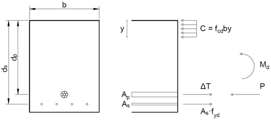
National and international standards such as EHE-08 [6], EC2 [11] or BPEL [12] propose their own procedure that helps the engineer at the design and/or at the analysis stage of the prestressed concrete structure. The methodology presented is similar in all of them and works through the analysis of the structure critical sections at Ultimate Limit State (ULS) (Figure 1). The prestressing steel effect is included in the section equilibrium equations (Equation 2.1 and 2.2) as a force applied at the tendon position and a bending moment, if needed, that accounts for hyperstatic effects [13].

Figure 1: Section analysis

$P=C-\Delta T-A_{s}f_{yd}$ $y={\dfrac {A_{p}f_{pyd}+A_{s}f_{yd}}{f_{cd}b}}={\dfrac {U_{p}+U_{s}}{f_{cd}b}}$

(2.1)

$M_{d}+P(d_{s}-d_{p})=C(d_{s}-{\frac {y}{2}})-\Delta T(d_{s}-d_{p})$ $U_{p}+U_{s}=f_{cd}bd_{s}\left(1-{\sqrt {1-{\dfrac {2\left(M_{d}+U_{p}\left(d_{s}-d_{p}\right)\right)}{f_{cd}bd_{s}^{2}}}}}\right)$

(2.2)

The rectangular section represented in Figure 1 and analysed in Equations 2.1 and 2.2 corresponds to the mid-span of a simple supported beam. Only prestressing steel and tensile reinforcing steel has been considered and the final equation has been written in the format that EHE-08 proposes for reinforced concrete rectangular sections subjected to flexure (EHE-08, Anejo 7. Cálculo simplicado de secciones en Estado Lite de Agotamiento frente a solicitaciones normales [6]) where ${\textstyle P}$ and ${\textstyle M_{d}}$ are acting forces on the beam section, i.e. the prestressing force and the bending moment due to external forces, respectively, ${\textstyle C}$, ${\textstyle A_{s}f_{yd}}$ and ${\textstyle \Delta T}$ are the resulting efforts due to external action, i.e. the compression in concrete due to ${\textstyle M_{d}}$ and the resulting tension in reinforcing and prestressing steel respectively, ${\textstyle f_{cd}}$, ${\textstyle f_{yd}}$ and ${\textstyle f_{pd}}$ are the strengths of concrete in compression, reinforcing steel and prestressing steel, respectively, ${\textstyle U_{p}}$ and ${\textstyle U_{s}}$ are notation parameters used in the same way that EHE-08 and the other variables are geometric parameters defined in Figure 1. The analysis would be complete when all the efforts have been studied, i.e. bending, shear and axial analysis.

Alternatively, codes provide stress limits at section level that must be respect for the design. These limits are grouped at Magnel equations (Equations 2.3, 2.4, 2.5 and 2.6) [14] which create the space of feasible solutions for a specified tendon geometry on elastic analysis. This theory has been already extended to non-linear behaviour needed when studying partially prestressed concrete sections [15].

Stress at transfer

$\sigma _{c,\,top}^{tra}=d{\frac {\gamma _{p}P}{A_{c,\,net}}}+{\dfrac {\gamma _{p}Pe_{net}v_{net}}{I_{c,\,net}}}+d{\frac {M_{sw}v_{net}}{I_{c,\,net}}}\geq \left\{{\begin{array}{c}-f_{ctmj}\\0\end{array}}\right.$

(2.3)

$\sigma _{c,\,bot.}^{tra}={\dfrac {\gamma _{p}P}{A_{c,\,net}}}+{\dfrac {\gamma _{p}Pe_{net}{v'}_{net}}{I_{c,\,net}}}+{\dfrac {M_{sw}{v'}_{net}}{I_{c,\,net}}}\leq 0.6f_{ckj}$

(2.4)

Stress at service

$\sigma _{c,\,top}^{ser}={\dfrac {\gamma _{p}P}{A_{c,\,hom}}}+{\dfrac {\gamma _{p}Pe_{hom}v_{hom}}{I_{c,\,hom}}}+{\dfrac {M_{char}^{SLS}v_{hom}}{I_{c,\,hom}}}\leq 0.6f_{ckj}$

(2.5)

$\sigma _{c,\,bot}^{ser}={\dfrac {\gamma _{p}P}{A_{c,\,hom}}}+{\dfrac {\gamma _{p}Pe_{hom}{v'}_{hom}}{I_{c,\,hom}}}+{\dfrac {M_{char}^{SLS}{v'}_{hom}}{I_{c,\,hom}}}\geq \left\{{\begin{array}{c}-f_{ctmj}\\0\end{array}}\right.$

(2.6)

In these equations, the stress is computed at the top and the bottom of the studied concrete section (${\textstyle i}$) and at transfer or service (${\textstyle j}$), i.e. ${\textstyle \sigma _{c,\,i}^{j}}$ generated by the prestressing force ${\textstyle P}$ factorized using ${\textstyle \gamma _{p}}$ and the corresponding bending moment ${\textstyle M}$ and it is compared with the specific concrete strength ${\textstyle f_{c},\,i}$ in each case. The other parameters are geometric variables: the section inertia (${\textstyle I}$), the section area (${\textstyle A}$) and the distance between the studied extreme of the section (top or bottom) and the neutral axis, i.e. ${\textstyle v}$ and ${\textstyle v'}$. And all them considering the net area or the full concrete.

In addition to the section equilibrium done at ULS, Service Limit State (SLS) is also checked at the codes approach. In fact, post-tensioned concrete structures are usually designed according to a limit in the maximum crack width (${\textstyle w_{max}}$) as shown in Table 2.1 obtained from EHE-08 and EC2.

In all the cases, the parameter that governs the design of a structure is the prestressing force value at the studied section. Codes provide the needed formulation that transforms the initial force applied at the anchorage area into the one transmitted along the studied element, i.e. prestressing losses calculation of post-tensioned elements [11,6,12].

Table. 1 Maximum crack width from EHE-08 and EC2

EHE 08
	$w_{max}\,[mm]$
	Reinforced members (quasi-permanent load combination)	Prestressed members (frequent load combination)
	0.4	0.2
IIa, IIb, H	0.3	0.2
IIIa, IIIb, IV, F, Qa	0.2	Decompression
IIIc, Qb, Qc	0.1
EC2
	$w_{max}\,[mm]$
	Reinforced members and prestressed members with unbounded tendons (quasi-permanent load combination)	Prestressed members with bounded tendons (frequent load combination)
	0.4	0.2
XC2, XC3, XC4	0.3	0.2
XD1, XD2, XD3, XS1, XS2, XS3		Decompression

Immediate losses

Immediate losses are those generated during the application of the prestressing force and at the wedge blocking operation. These losses have different origin and are studied independently, differentiating between:

• Friction losses, $\Delta P_{\mu }$. The contact between tendons and ducts prevent the force transmission from the active end, where tendons are being tensioned. The expression proposed at codes that calculates these losses from the applied force (${\textstyle P_{0}}$) is:

$\Delta P_{\mu }=P_{0}\left(1-e^{-\left(\mu \alpha {+}kx\right)}\right)$

(2.7)

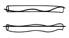
The variables that control force losses in Equation 2.7 are ${\textstyle \mu }$ and ${\textstyle k}$. This evidences the existence of two kind of friction that have different nature. ${\textstyle \mu }$ is related to the contact produced at curve zones of the tendon path and therefore it appears next to ${\textstyle \alpha }$, that is the total angular displacement. On the other hand, ${\textstyle k}$ is related to a friction produced by an unintentional angular displacement at straight areas of the tendon path and so it is proportional to the length ${\textstyle x}$ (Figure 2).

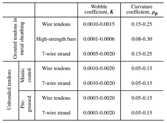
Values for these two parameters are obtained experimentally. Standards provide their own proposal depending on the type of steel that is used, the kind of bounding that is used, the duct diameter, etc. (Figure 3).

]

Figure 2: Graphical description for $k$ coefficient [10]

]

Figure 3: $\mu$ and $k$ values from the American Concrete Institue (ACI 318-05) [16]

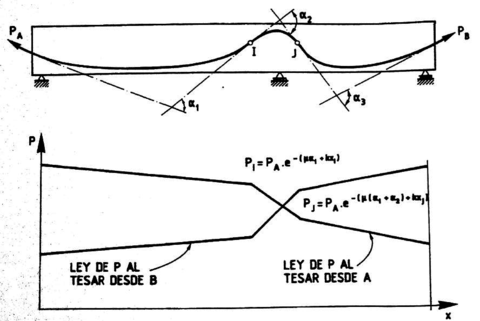
Equation 2.7 is usually applied discreetly at sections with curvature changes and then these values are linearly interpolated for the whole structure. A visual example that helps to fully comprehend the result that could be obtained using the previous expression is shown at Figure 4, where the prestressing force distribution after friction losses is drawn for a three-span continuous beam.

]

Figure 4: Prestressing force distribution after friction losses [10]

• Losses due to wedge draw-in of the anchorage devices, $\Delta P_{a}$. When post-tensioned tendons are anchored, some of the force applied during the post-tensioning operation is lost. It is important to minimize the amount of stress lost and the affected length by this phenomenon. Expression 2.8 [17] point out the variables involved in the problem:

$a=\int _{0}^{L}{\dfrac {\Delta P_{a}(x)}{E_{p}A_{p}}}dx$

(2.8)

Where ${\textstyle A_{p}}$ and ${\textstyle E_{p}}$ are the prestressing steel total area and longitudinal elastic modulus, ${\textstyle a}$ is the pull-in at wedge blocking and ${\textstyle L}$ is the tendon length. Considering that the function that describes the force loss due to wedge blocking behaves in the same way than the one used for friction losses (Figure 5), then Equation 2.8 can be rewritten as:

$a={\dfrac {S}{A_{p}E_{p}}}={\dfrac {\Delta P_{a}l_{p}}{2E_{p}A_{p}}}={\dfrac {P_{A}\left[1-e^{-\left(\mu \alpha {+}kl_{p}\right)}\right]l_{p}}{A_{p}E_{p}}}$

(2.9)

Where ${\textstyle P_{A}}$ is the applied force at the active end of the tendon and ${\textstyle l_{p}}$ is the affected length due to anchorage operation.

]

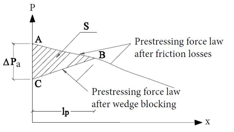Figure 5: Prestressing force redistribution after wedge blocking [17]

• Losses due to concrete instantaneous deformation, $\Delta P_{el}$. The stress transmission from tendons to concrete during anchorage operations generates a deformation in concrete that reduces the prestressing force at tendon. This is only a problem when several tendons are tensioned and the operation cannot be done simultaneously. The consecutive concrete deformations generate force losses at tendons that have been previously anchored.

Standards provide formulas with similar format to Equation 2.10, which consider that concrete deformations remain in the elastic domain.

$\Delta P_{el}=A_{p}E_{p}\sum {\left[{\dfrac {j\,\Delta \sigma _{c}(t)}{E_{cm}(t)}}\right]}$

(2.10)

Where ${\textstyle A_{p}}$ and ${\textstyle E_{p}}$ are again the prestressing steel total area and the longitudinal elastic modulus, ${\textstyle E_{cm}(t)}$ is the concrete elastic modulus at the age that tension operations take place, ${\textstyle \Delta \sigma _{c}(t)}$ is the variation of concrete stress at the centre of gravity of the tendons applied at time ${\textstyle t}$ and ${\textstyle j}$ is a coefficient equal to ${\textstyle {\dfrac {n-1}{2n}}}$ as shown by Aguado, Mirambell, Murcia and Marí (1983) [18] that can be approximated to ${\textstyle j=0.5}$ when the number of tendons, ${\textstyle n}$, is high.

According to Murcia, Aguado and Marí (1993) [10] and the EHE-08 [6], ${\textstyle \Delta \sigma _{c}(t)}$ value can be computed as ${\textstyle P_{0}-\Delta P_{\mu }-\Delta P_{a}}$ and should be checked the transfer state where only prestressing force and self weight are applied because this situation could be more restrictive [10].

The formulas introduced in this section are valid only for post-tensioned concrete structures, which are the object of study of this monograph. Pre-tensioned concrete structures are treated in a different way.

Time dependent losses

Once the prestressing operations have taken place, rheological mechanisms start to develop which lead to a generalised stress loss in the prestressing system. These procedures are known as time dependent losses, which are originated by creep and shrinkage at concrete and relaxation at the prestressing system.

The incorporation of these mechanisms into the structure analysis is complex due to the existing interdependence between them, e.g. shrinkage generates stress losses that affect creep and steel relaxation procedures. In practice standards try to simplify these calculations by uncoupling the mechanisms and study them independently [12] or by using specific formulation depending on the structure conditions [19]. EC2 and EHE-08, for example, propose a simplified method based on the ageing coefficient (${\textstyle \chi }$):

$\Delta P_{c+s+r}=A_{p}{\dfrac {\varepsilon _{cs}+E_{p}+0.8\Delta \sigma _{pr}+{\dfrac {E_{p}}{E_{cm}}}\varphi (t,t_{0})\sigma _{c,QP}}{1+{\dfrac {E_{p}}{E_{cm}}}{\dfrac {A_{p}}{A_{c}}}\left(1+{\dfrac {A_{c}}{I_{c}}}z_{cp}^{2}\right)\left[1+\chi \varphi (t,t_{0})\right]}}$

(2.11)

Where:

• is the force loss due to creep, shrinkage and steel relaxation at location ${\textstyle x}$, at time ${\textstyle t}$
• shrinkage strain
• Young modulus for the prestressing steel
• Young modulus for the concrete
• stress loss due to steel relaxation
• is the creep coefficient at a time ${\textstyle t}$ and load application at time ${\textstyle t_{0}}$
• concrete stress due to the prestressing effect, the self-weight and the dead loads. This stress is measured at the centre of gravity of the prestressing steel area (${\textstyle A_{p}}$).
• is tendons total area at the location ${\textstyle x}$
• is concrete total area at the location ${\textstyle x}$
• is the moment of inertia of the concrete section
• is the distance between the centre of gravity of the tendons and the concrete section
• is the ageing coefficient that can be approximated as ${\textstyle \chi =0.8}$ when time tends to infinity

2.2 FEM approach

The use of numerical techniques in the structural analysis field has provided researchers a powerful tool that permits a global study of the structure. The accuracy level that these methodologies can achieve and the potential for solving complex cases make them attractive for many research lines.

Despite this, these computational techniques have also drawbacks. Therefore, it is important to know when to use them and which is the best type of analysis to be performed. For example, regions with discontinuities in geometry or actions, also known as D-regions [11,6], not necessarily have to be designed using a finite element (FE) model, strud-and-tie method [20] can be used instead. Another example is the case of bridges. For these structures it is not always needed a 3-D FEM design, many bridge decks have been designed using simplified methodologies such as the Grillage method [21].

Prestressed concrete structures can be studied using the FEM and the interest on its use increases as the structure becomes more complex. There is no standardised procedure for the analysis of these structures, research papers can show the wide range of options that exist [22,23,24,25]. The difficulties that arise from their analysis are originated by the coexistence of three different materials: concrete, reinforcing steel and prestressing steel.

While the concrete modelization is similar in all cases, the way that strands and tendons are included in the FE analysis make the difference between the existing approaches. Some of these are:

3-D solid elements

The use of 3-D elements for the prestressing steel modelization (see Figure 6) is used mainly in pre-tensioned beams [25] where one of the main stress transfer mechanisms between strands and concrete (Hoyer effect [26]) is also of 3-D nature.

]

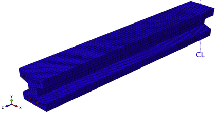Figure 6: Tendon modelization using 3-D solid elements [25]

Modelling through 3-D elements introduces the need for using rectangular equivalent cross section for the prestressing steel but this allows an easy optimization of the contact between concrete and steel elements.

The use of this modelization scheme restricts the range of structures that can be studied. In fact, only construction with straight tendons are valid for this approach, i.e. only pre-tensioned structures or simple post-tensioned ones.

Truss discrete elements

This is probably the most extended option when using FEMs. In this case, tendons are simulated using trusses, which are linked somehow to the 3D FE mesh of the structure and the prestressing effect is considered as an imposed strain to the bar elements.

At the beginning, this methodology was only used in small structures because it had a big restriction: the FE mesh depended on the trusses path. This was because the methodology took into account the tendons effect by coupling the strengths of the prestressing steel and the concrete at the FE mesh nodes [22,23,24].

Building a mesh adjusted to the tendons path is only possible in those cases where there are few tendons or when their geometry is simple, therefore this technique could not be used in most of the real life scenarios.

Despite this, it exists an approach introduced by the commercial code Abaqus [27] that solves this big restriction. It is currently used in most of the prestressed concrete simulations and it is based on the so called embedded elements [28].

]

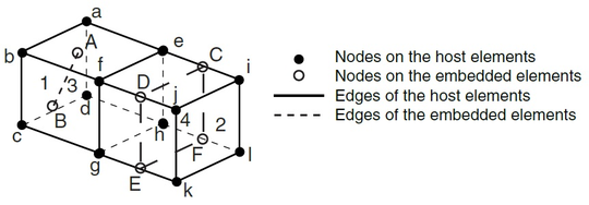Figure 7: Abaqus example of an embedded element [28]

Figure 7 shows an example of two embedded elements. This approach constrains the degrees of freedom of the embedded element to the closest nodes of the hosting element using weight factors, which are determined based on their geometric location. This technique is not limited to truss elements. It can be used for membranes for example.

In spite of this improvement, the procedure has limitations. This is, in fact, an interpolation technique, where the results obtained in the analysis for the 3D FE mesh are used to compute results for the embedded elements. In the scenario of prestressed concrete structures, where the non-linear behaviour of concrete and the time dependent mechanisms of prestressing steel have to be considered, the use of this approach only solves partially the problem and there are still things to improve.

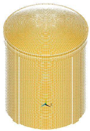
Figure 8a shows an example of a structure solved using Abaqus embedded elements.

Truss smeared elements

This last approach is usually applied for big structures where using the other techniques is not feasible. In these cases, tendons are introduced in the analysis as embedded reinforcement, i.e. the prestressing steel only appears in the analysis as an increment of the strength of the concrete FE. Therefore, this methodology introduces big simplifications in the analysis and has to be used carefully.

In fact, this approach is commonly used in current analysis to account for the reinforcing steel effect. In real prestressed concrete structures, this material is distributed more or less uniformly in specific directions (longitudinal rebars and shear reinforcement), which constitutes the perfect scenario to apply this approach.

This is the strategy followed by Tavakkoli, Kianoush et al. (2017) [24] for the analysis of the reactor containment building shown in Figure 8b.

]	]
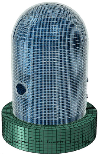(a) FE mesh of a containment building analysed using Abaqus [23]	(b) Containment building model where truss smeared elements are used for rebars [24]
Figure 8: Examples where tendons and reinforcement have been modelled using truss elements

3 Modelization through the FEM

This section intends to introduce the FEM, which is used as a base for the application of the SP RoM. In particular, the text will be focused on the development of the three-dimensional formulation using an elastic constitutive model.

3.1 Introduction to FEM

The FEM is a numerical method used in the analysis of structures to give an approximate solution to the differential equations that govern the problem. The use of this technique allows obtaining a continuum solution and therefore, getting a global vision of the structural behaviour. This is very attractive for studying the response of complex areas, e.g. D-regions or full structures with non-intuitive behaviour.

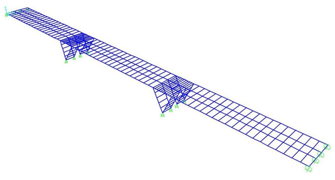
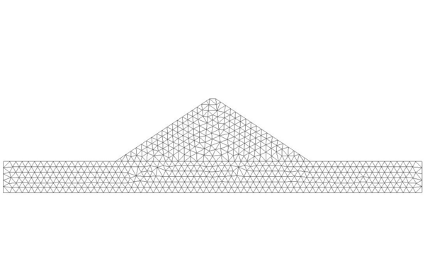
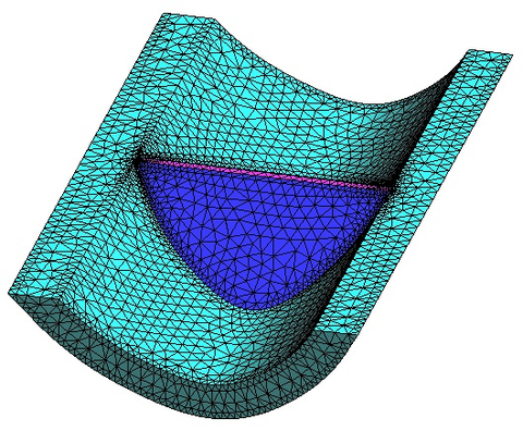
This methodology is build around the concept of FEs. These should be understood as each division in which the structure is split and analysed. Depending on the analysis nature, FEs can be 1-D (truss elements), 2-D (triangular or quadrilateral elements) or 3-D (tetrahedral or hexahedral elements) (Figure 9). For the development of the approach introduced at this monograph, hexahedral elements are needed, therefore the formulation presented in this section is the one used for 3-D problems.

(a) Bridge modelled using truss elements
(b) Dam mesh using triangle elements	(c) Dam mesh using tetrahedral elements
Figure 9: Examples of the type of mesh that can be build using the FEM

In the end, the FEM solves the whole structure working through many simple element equations over many small domains, i.e. the FEs. The procedure followed while performing a simulation using the FEM can be summed up in the following steps [29,30]:

• Generate an appropriate model. The first thing to be done is a correct modelization of the problem. This includes:

• Build a geometrical model that represents the studied structure, paying attention to the possibility of including simplifications that could lighten the simulation, e.g. symmetries, plane stress case, plane strain case [1], etc.
• Consider how the real constraints and the applied forces should be included in the model and so define the boundary conditions.
• Apply the correct material properties to the model.
• Define the scope of the analysis, e.g. small or large displacements, static or dynamic analysis, etc.
• Generate the mesh of FEs. The model is discretized in sub-domains in which the problem is solved locally. This mesh can be structured, unstructured or semi-structured [31] and coarse or fine as needed.
• Define the equilibrium condition through the Principle of Virtual Work (PVW). The PVW is a necessary and sufficient condition for the equilibrium of the whole analysed structure or any of its sub-domains [1].
• Compute the stiffness matrix ${\textstyle K^{e}}$ and load vector ${\textstyle f^{e}}$ for each element. These are obtained from the PVW expression in terms of the nodal displacement of the FE mesh, i.e. ${\textstyle K^{e}\,a^{e}-f^{e}=\Delta f^{e}}$. This expression will be analysed later on.
• Obtain the global stiffness matrix (${\textstyle K}$) and the global load vector (${\textstyle f}$). These are obtained assembling all the ${\textstyle K^{e}}$'s and ${\textstyle f^{e}}$'s that come from the FE's analysis.
• Solve the system of equations ${\textstyle K\,a=f}$. The unknown displacement ${\textstyle a}$ is obtained.
• Result assessment. Once the system of equations has been solved and the displacement vector ${\textstyle a}$ has been found out, strains and stresses can be evaluated at each element. Also reactions at the restraint nodes can be computed. These results can be load into the model and presented graphically to their assessment. This is known as post-processing step.
• Possible modifications. The last step of the FEM consists in considering possible changes that could improve the analysis performed. For example, consider a finer FE mesh or changing the FE typology.

Once the general procedure has been introduced, it is important to go in depth with the 3-D formulation and introduce the main concepts that are relevant for the monograph.

3.2 FEM three dimensional formulation

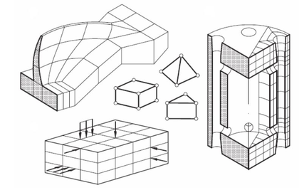
The use of a 3-D analysis using the FEM is usually related to the impossibility of using less costly procedures. This is the case of structures with irregular shapes and situations where the load patterns are arbitrary or the material properties are heterogeneous (Figure 10). In general, this is the case of post-tensioned concrete structures. Thus, the understanding of the subsequent formulation is essential for the progress of this dissertation.

]

Figure 10: Structures which require a 3-D analysis [1]

Isotropic elasticity theory is used at this stage in order to facilitate introducing the 3-D formulation although any other constitutive model could have been used instead.

Before dealing with the equations derived from the FEM, the formulas that control the 3-D elasticity problem must be introduced.

3.2.1 Displacement, strain and stress field

In a 3-D solid, the movement description of any point that belongs to that solid is done through the three components of the displacement vector:

$\mathbf {u} =\left[u,v,w\right]^{T}$

(3.1)

Where ${\textstyle u}$, ${\textstyle v}$ and ${\textstyle w}$ are the displacement components of vector ${\textstyle \mathbf {u} }$ in the directions of a cartesian reference system ${\textstyle x}$, ${\textstyle y}$ and ${\textstyle z}$, respectively.

The strain field is then defined through the six strain components of the 3-D elasticity:

${\boldsymbol {\varepsilon }}=\left[\varepsilon _{x},\varepsilon _{y},\varepsilon _{z},\gamma _{xy},\gamma _{xz},\gamma _{yz}\right]^{T}$ $=\left[{\dfrac {\partial u}{\partial x}},{\dfrac {\partial v}{\partial y}},{\dfrac {\partial w}{\partial z}},{\dfrac {\partial u}{\partial y}}+{\dfrac {\partial v}{\partial x}},{\dfrac {\partial u}{\partial z}}+{\dfrac {\partial w}{\partial x}},{\dfrac {\partial v}{\partial z}}+{\dfrac {\partial w}{\partial y}}\right]^{T}$

(3.2)

Where ${\textstyle \varepsilon _{x}}$, ${\textstyle \varepsilon _{y}}$ and ${\textstyle \varepsilon _{z}}$ are the normal strains and ${\textstyle \gamma _{xy}}$, ${\textstyle \gamma _{xz}}$ and ${\textstyle \gamma _{yz}}$ are the tangential strains. These can be written in terms of the displacement vector components as shown in Equation 3.2.

Likewise, stress field can be defined through the six stress components as:

${\boldsymbol {\sigma }}=\left[\sigma _{x},\sigma _{y},\sigma _{z},\tau _{xy},\tau _{xz},\tau _{yz}\right]^{T}$

(3.3)

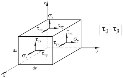
Where ${\textstyle \sigma _{x}}$, ${\textstyle \sigma _{y}}$ and ${\textstyle \sigma _{z}}$ are the normal stresses and ${\textstyle \tau _{xy}}$, ${\textstyle \tau _{xz}}$ and ${\textstyle \tau _{yz}}$ are the tangential stresses defined according to the sign criterion shown in Figure 11.

]

Figure 11: Sign criterion for the stresses in a 3-D solid [1]

Finally, the relation between the strain and stress fields is expressed through a constitutive equation. In terms of isotropic elasticity this relationship can be written as:

${\boldsymbol {\sigma }}=\mathbf {C} \left({\boldsymbol {\varepsilon }}-{\boldsymbol {\varepsilon ^{0}}}\right)+{\boldsymbol {\sigma ^{0}}}$

(3.4)

Where the isotropic constitutive matrix (${\textstyle \mathbf {C} }$) depends only on two material parameters, i.e. the Young modulus (${\textstyle E}$) and the Poisson's ratio (${\textstyle \nu }$). Therefore, the symmetric tensor ${\textstyle \mathbf {C} }$ is given by:

$\mathbf {C} ={\dfrac {E\left(1-\nu \right)}{\left(1+\nu \right)\left(1-2\nu \right)}}\left[{\begin{matrix}1&{\dfrac {\nu }{1-\nu }}&{\dfrac {\nu }{1-\nu }}&0&0&0\\&1&{\dfrac {\nu }{1-\nu }}&0&0&0\\&&1&0&0&0\\&&&{\dfrac {1-2\nu }{2\left(1-\nu \right)}}&0&0\\&\mathrm {Sym.} &&&{\dfrac {1-2\nu }{2\left(1-\nu \right)}}&0\\&&&&&{\dfrac {1-2\nu }{2\left(1-\nu \right)}}\end{matrix}}\right]$

(3.5)

And the initial strain vector (${\textstyle {\boldsymbol {\varepsilon ^{0}}}}$) due to thermal strains is:

${\boldsymbol {\varepsilon ^{0}}}=\alpha \left(\Delta T\right)\left[1,1,1,0,0,0\right]^{T}$

(3.6)

3.2.2 Equilibrium equation in 3-D (PVW)

Equilibrium is guaranteed through the PVW [1] expression that for 3-D solids is:

$\iiint _{V}\delta {\boldsymbol {\varepsilon }}^{T}{\boldsymbol {\sigma }}\,dV=\iiint _{V}\delta \mathbf {u} ^{T}\mathbf {b} \,dV+\iint _{A}\delta \mathbf {u} ^{T}\mathbf {t} \,dA+\sum _{i}\delta \mathbf {a} _{i}^{T}\mathbf {p} _{i}$

(3.7)

Where ${\textstyle \delta {\boldsymbol {\varepsilon }}}$ and ${\textstyle \delta \mathbf {u} }$ are respectively the virtual strains and virtual displacements, ${\textstyle V}$ and ${\textstyle A}$ are respectively the volume and the surface in which the body forces (${\textstyle \mathbf {b} =\left[b_{x},b_{y},b_{z}\right]^{T}}$) and the surface tractions (${\textstyle \mathbf {t} =\left[t_{x},t_{y},t_{z}\right]^{T}}$) are applied and ${\textstyle \mathbf {p} _{i}=\left[P_{x_{i}},b_{y_{i}},b_{z_{i}}\right]^{T}}$ are the point loads acting at node ${\textstyle i}$. It is important to notice that ${\textstyle C^{0}}$ continuity is required for the finite element approximation because only first derivatives of the displacement are involved in Equation 3.7.

3.2.3 Finite element formulation. The 8-noded hexahedra

Once the equilibrium expression has been defined and all the involved variables have been introduced analytically, the FEM can be applied. For the purpose of this tmonograph, hexahedral elements are used and so it is interesting to present the finite element formulation using these elements.

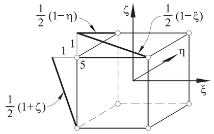
There are several type of hexahedral elements but the current code used to run the methodology presented in this monograph is prepared to work using 8-noded linear hexahedras (Figure 12).

]

Figure 12: Example of a 8-noded hexahedra with linear shape function [1]

Shape functions

Shape functions (${\textstyle N_{i}^{\left(e\right)}}$) are polinomial interpolating functions defined over the domain of each element in the FE mesh that take the value one at node ${\textstyle i}$ and zero at all other nodes. Therefore, Equation 3.11 satisfies ${\textstyle u\left(x_{i}\right)=u_{i}^{\left(e\right)}}$.

For 8-noded linear hexahedra, the nodal shape function can be written as:

$N_{i}\left(\xi ,\eta ,\zeta \right)={\dfrac {1}{8}}\left(1+\xi _{i}\xi \right)\left(1+\eta _{i}\eta \right)\left(1+\zeta _{i}\zeta \right)$

(3.8)

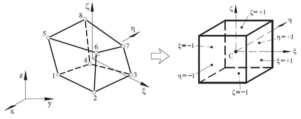
Where ${\textstyle \xi ,\eta ,\zeta }$ are the natural coordinates as shown in Figure 13. This expression satisfies the two necessary conditions of a shape function: condition of nodal compatibility (Equation 3.9) and rigid body condition (Equation 3.10).

$N_{i}\left(\xi _{j},\eta _{j},\zeta _{j}\right)=\left\{{\begin{array}{lll}1&\mathrm {if} &i=j\\0&\mathrm {if} &i\neq j\end{array}}\right.$

(3.9)

$\sum _{i=1}^{n}N_{i}\left(\xi ,\eta ,\zeta \right)=1$

(3.10)

Further details about the procedure to be followed when obtaining shape functions can be found in specialised bibliography [29,1].

]

Figure 13: Example of a generic hexahedra FE and its normalized geometry [1]

Discretization of the displacement field

Considering a 3-D solid discretized into 8-noded hexahedras, the displacement field within each element can be expressed as:

$\mathbf {u} =\left\lbrace {\begin{matrix}u\\v\\w\end{matrix}}\right\rbrace =\sum _{i=1}^{8}\mathbf {N} _{i}\mathbf {a} _{i}^{\left(e\right)}=\mathbf {N} \mathbf {a} ^{\left(e\right)}$

(3.11)

Where

$\mathbf {N} =\left[\mathbf {N} _{1},\mathbf {N} _{2},\dots ,\mathbf {N} _{8}\right]\qquad \qquad \mathbf {N} _{i}=\left[{\begin{matrix}N_{i}&0&0\\0&N_{i}&0\\0&0&N_{i}\end{matrix}}\right]$

(3.12)

and

$\mathbf {a} ^{\left(e\right)}=\left\lbrace {\begin{matrix}\mathbf {a} _{1}^{\left(e\right)}\\\mathbf {a} _{2}^{\left(e\right)}\\\vdots \\\mathbf {a} _{8}^{\left(e\right)}\end{matrix}}\right\rbrace \qquad \qquad \mathbf {a} _{i}^{\left(e\right)}=\left\lbrace {\begin{matrix}u_{i}\\v_{i}\\w_{i}\end{matrix}}\right\rbrace$

(3.13)

are the shape function matrix and the displacement vector for each element and a node ${\textstyle i}$.

Discretization of the strain field

The new expression for representing the strain field in terms of the FEM is obtained combining Equation 3.2 and Equation 3.11. The result is:

${\boldsymbol {\varepsilon }}=\sum _{i=1}^{8}\left\lbrace {\begin{matrix}{\dfrac {\partial N_{i}}{\partial x}}u_{i}\\{\dfrac {\partial N_{i}}{\partial y}}v_{i}\\{\dfrac {\partial N_{i}}{\partial z}}w_{i}\\{\dfrac {\partial N_{i}}{\partial y}}u_{i}+{\dfrac {\partial N_{i}}{\partial x}}v_{i}\\{\dfrac {\partial N_{i}}{\partial z}}u_{i}+{\dfrac {\partial N_{i}}{\partial x}}w_{i}\\{\dfrac {\partial N_{i}}{\partial z}}v_{i}+{\dfrac {\partial N_{i}}{\partial y}}w_{i}\\\end{matrix}}\right\rbrace =\sum _{i=1}^{8}\mathbf {B} _{i}\mathbf {a} _{i}^{\left(e\right)}=\sum _{i=1}^{8}\mathbf {B} \mathbf {a} ^{\left(e\right)}$

(3.14)

Where ${\textstyle \mathbf {B} }$ is the element strain matrix that can be written as:

$\mathbf {B} =\left[\mathbf {B} _{1},\mathbf {B} _{2},\dots ,\mathbf {B} _{8}\right]$

(3.15)

and ${\textstyle \mathbf {B} _{i}}$ is the strain matrix of the node ${\textstyle i}$:

$\mathbf {B} _{i}=\left[{\begin{matrix}{\dfrac {\partial N_{i}}{\partial x}}&0&0\\0&{\dfrac {\partial N_{i}}{\partial y}}&0\\0&0&{\dfrac {\partial N_{i}}{\partial z}}\\{\dfrac {\partial N_{i}}{\partial y}}&{\dfrac {\partial N_{i}}{\partial x}}&0\\{\dfrac {\partial N_{i}}{\partial z}}&0&{\dfrac {\partial N_{i}}{\partial x}}\\0&{\dfrac {\partial N_{i}}{\partial z}}&{\dfrac {\partial N_{i}}{\partial y}}\end{matrix}}\right]$

(3.16)

Obtaining the shape function derivatives with respect to cartesian coordinates requires the use of the chain rule because they are expressed in normalized coordinates.

Equilibrium equation in terms of the FEM

Finally, the PVW expression (Equation 3.7) can be written using the described formulas (Equations 3.8 to 3.16). Therefore:

$\iiint _{V}\mathbf {B} ^{T}{\boldsymbol {\sigma }}\,dV=\iiint _{V}\mathbf {N} ^{T}\mathbf {b} \,dV+\iint _{A}\mathbf {N} ^{T}\mathbf {t} \,dA+\Delta \mathbf {f} ^{\left(e\right)}$

(3.17)

Where it has been taken into account that virtual strain and virtual displacement are:

$\delta {\boldsymbol {\varepsilon }}=\mathbf {B} \delta \mathbf {a} \qquad \qquad \delta \mathbf {u} =\mathbf {N} \delta \mathbf {a}$

(3.18)

Equation 3.17 sets the equilibrium of internal and external forces at each element. ${\textstyle \iiint _{V}\mathbf {B} ^{T}{\boldsymbol {\sigma }}\,dV}$ is the internal nodal force vector for the element ${\textstyle f_{int}^{\left(e\right)}}$ and the term ${\textstyle \iiint _{V}\mathbf {N} ^{T}\mathbf {b} \,dV+\iint _{A}\mathbf {N} ^{T}\mathbf {t} \,dA}$ is the external load vector, which gives the information of the forces applied in each element ${\textstyle f_{ext}^{\left(e\right)}}$. Thus, this expression is equivalent to ${\textstyle f_{int}^{\left(e\right)}-f_{ext}^{\left(e\right)}=\Delta \mathbf {f} ^{\left(e\right)}}$. Finally, ${\textstyle \Delta \mathbf {f} ^{\left(e\right)}}$ is the vector of equilibrating nodal forces, i.e. it has the information that guarantees the equilibrium of each element. Therefore, when the assembling is done it only contains the information related with the reaction forces.

Equation 3.17 can be rewritten as a system of equations considering the relation between strain and stress given by Equation 3.4:

$\iiint _{V}\mathbf {B} ^{T}\mathbf {C} \mathbf {B} \,dV\mathbf {a} ^{\left(e\right)}-\iiint _{V}\mathbf {B} ^{T}\mathbf {C} {\boldsymbol {\varepsilon }}^{0}\,dV+$ $+\iiint _{V}\mathbf {B} ^{T}\mathbf {C} {\boldsymbol {\sigma }}^{0}\,dV-\iiint _{V}\mathbf {N} ^{T}\mathbf {b} \,dV-\iint _{A}\mathbf {N} ^{T}\mathbf {t} \,dA=\Delta \mathbf {f} ^{\left(e\right)}$

(3.19)

Using the stiffness matrix (${\textstyle \mathbf {K} ^{\left(e\right)}}$) and the equivalent force vector (${\textstyle \mathbf {f} ^{\left(e\right)}}$) concepts, this equation is equivalent to:

$\mathbf {K} ^{\left(e\right)}\mathbf {a} ^{\left(e\right)}-\mathbf {f} ^{\left(e\right)}=\Delta \mathbf {f} ^{\left(e\right)}$

(3.20)

Where:

$\mathrm {Stiffness\,matrix:} \qquad \mathbf {K} ^{\left(e\right)}=\iiint _{V}\mathbf {B} ^{T}\mathbf {C} \mathbf {B} \,dV$ $\mathrm {Equivalent\,force\,vector:} \qquad \mathbf {f} ^{\left(e\right)}=\iiint _{V}\mathbf {B} ^{T}\mathbf {C} {\boldsymbol {\varepsilon }}^{0}\,dV-\iiint _{V}\mathbf {B} ^{T}\mathbf {C} {\boldsymbol {\sigma }}^{0}\,dV+$ $\qquad +\iiint _{V}\mathbf {N} ^{T}\mathbf {b} \,dV+\iint _{A}\mathbf {N} ^{T}\mathbf {t} \,dA$

Equation 3.20 sets the problem to be solved element by element and the global linear system of equation:

$\mathbf {K} \mathbf {a} =\mathbf {f}$

(3.21)

can be obtained assembling the ${\textstyle \mathbf {K} ^{\left(e\right)}}$ and ${\textstyle \mathbf {f} ^{\left(e\right)}}$ contributions.

3.3 Solving the system of equations

At this stage of the analysis, the system of equations must be solved in order to finally obtain the strain values, the stress values, etc. at the studied structure. The procedure to be followed now depends on the type of analysis performed: linear or non-linear.

Prestressed concrete structures are a clear example of non-linear behaviour. The main procedures that can drive the structure in this range are related with the material degradation (damage in concrete, plasticity in steel, etc.) and the unavoidable changes that take place with time (creep, stress relaxation in prestressing steel, etc.). Therefore, for the purpose of this monograph, a strategy to solve non-linear systems of equations must be followed.

In these problems, the existence and uniqueness of the solution is not guaranteed. This makes it necessary to use an approach that follows the equilibrium path by using incrementation or continuity, which gives more information on the mechanical behaviour of the system and it also helps tracing the equilibrium path near critical points and facilitates convergence.

There are several techniques that can be used in order to solve a non-linear system of equations, which can be classified in explicit or implicit methods. For the purpose of this monograph an implicit approach has been used due to the robustness and the stability of these mechanisms: the Newton-Raphson technique [32].

This iterative method assumes that, in a static analysis, the equilibrium equation has the general form:

$\Delta \mathbf {f} =\left[\mathbf {f} ^{int}\left(\mathbf {u} \right)\right]^{t+\Delta t}-\left[\mathbf {f} ^{ext}\right]^{t+\Delta t}=\mathbf {0}$

(3.22)

Where ${\textstyle \mathbf {f} ^{int}}$ and ${\textstyle \mathbf {f} ^{ext}}$ are the internal and external force vectors that have already been introduced.

Equation 3.22 is the objective function and thus, the algorithm will iterate until this condition is reached. This expression can be written using the Taylor approximation series truncated at the second term:

$0={^{i+1}}\left[\Delta \mathbf {f} \right]^{t+\Delta t}\simeq {^{i}}\left[\Delta \mathbf {f} \right]^{t+\Delta t}+{^{i}}\left[{\dfrac {\partial \Delta \mathbf {f} }{\partial \mathbf {u} }}\right]^{t+\Delta t}{^{i+1}}\left[\Delta \mathbf {u} \right]^{n+1}=$ $={^{i}}\left[\Delta \mathbf {f} \right]^{t+\Delta t}+{^{i}}\left[\mathbf {J} \right]^{t+\Delta t}{^{i+1}}\left[\Delta \mathbf {u} \right]^{t+\Delta t}$

(3.23)

Where ${\textstyle i}$ represents the iteration counter and ${\textstyle t}$ is the current time. This is solved inverting the Jacobian operator:

${^{i+1}}\left[\Delta \mathbf {u} \right]^{t+\Delta t}=-\left({^{i}}\left[\mathbf {J} \right]^{t+\Delta t}\right)^{-1}{^{i}}\left[\Delta \mathbf {f} \right]^{t+\Delta t}$

(3.24)

The Jacobian matrix is the tangent stiffness matrix if the problem is static, which is linear, i.e. ${\textstyle \mathbf {J} =\mathbf {K} _{tang}}$.

Finally, the displacement at the end of each iteration is written as:

${^{i+1}}\left[\mathbf {u} \right]^{t+\Delta t}={^{i}}\left[\mathbf {u} \right]^{t+\Delta t}+{^{i+1}}\left[\Delta \mathbf {u} \right]^{t+\Delta t}$

(3.25)

Figure 14 shows an overview of what the Newton-Raphson is doing at each step of the calculation.

]

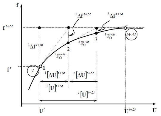Figure 14: Newton-Raphson technique scheme [32]

This method has quadratic convergence which is really helpful for the calculation but it also has some drawbacks that must be considered:

• Jacobian operator cost. This approach computes the Jacobian matrix at each iteration which is usually costly. There are alternatives that can be used instead (modified Newton-Raphson) but then the speed of convergence is lost. Thus, it is important to know which situation is better.
• Antisymmetric Jacobian operators. There are scenarios where the Jacobian matrix is not symmetric and so its inversion is difficult.
• The proximity of the studied point. The speed of convergence depends on whether the point being studied is close or far away from the previous one. Thus, quadratic convergence is only achieved when the solution point is close to the previous one.
• The presence of local extrema. When local extrema are found, the algorithm can lose information and has problems in leaving them afterwards. This can be solved using auxiliary techniques, such as displacement-controlled methods (arc-length).

4 Serial-Parallel Rule of Mixtures

Now that the algorithm applied at the analysis of the prestressed concrete structure, the FEM, has been introduced, it is important to establish how the structure is considered within the study. This is done through the Serial-Parallel Rule of Mixtures (SP RoM). While the origin of this technique dates back to the end of the nineteenth century, its use in the assessment of prestressed concrete structures is novel.

In this section, the bases of the methodology will be introduced in order to fully comprehend the procedure followed during the structural modelization. Furthermore, this will show the potential of the algorithm in comparison with the procedures introduced in Chapter 2.

4.1 Modelling composites - RoM evolution

Nowadays, there are several techniques that allow the modelization of composite materials. These differ among them in terms of the scale used, giving rise to micro-mechanic, macro-mechanic or homogenization methods [8].

The SP RoM can be included in the category of Micro-Mechanic Methods, specifically it can be catalogued as a Mean Field Method (MFM). It is the result of a century of evolution of the original idea but the bases have the essence of these methodologies. Micro-Mechanic Models study the strain and stress fields at a micro-scale level in order to build the constitutive laws and MFMs add to this conception the fact that:

• Mean stresses and strains at each component of the composite material are representative of the constituent behaviour.
• Stresses and strains at the composite material are related with the stresses and strains at each constituent.

The origin of the RoM theory is attributed to Voigt [33] and Reuss [34] who developed a methodology for computing the elastic properties of a composite material. The procedure was quickly extended to the calculation in the non-linear domain [35,36]. At that stage, the RoM depended only on one micro-mechanical property, the volumetric contribution of each component in relation to the whole composite material. This was the only variable when computing global properties from the ones calculated for the material constituents.

This approach evolved in 1960 towards a new version of the RoM known as Classical Mixing Theory (CMT). This new approach allowed the analysis of composite structures at the non-linear domain. Despite this, it had a big limitation: the isostrain hypothesis, i.e. all the coexisting materials in a point of the composite were subjected to the same strain field (pure parallel behaviour).

This limitation could be overcome by using a mixture of the isostrain condition (pure parallel behaviour) and the isostress condition (pure serial behaviour), which would had allowed the simulation of the real behaviour of the composite material. This change was not made effective until the end of 90's, leading to the SP RoM. The version of the methodology used in this monograph is the consequence of twenty years of evolution of the theory [37,8].

4.2 SP RoM formulation

The formulation presented in this section will be of assistance in order to understand how composite properties can be obtained from the components properties. Despite this, these equations are only valid for the case of small strains.

Notice that the SP RoM is a MFM and therefore, the strain and stress values calculated here are always mean values of these fields:

${\bar {\boldsymbol {\varepsilon }}}:={\dfrac {\int _{\Omega }{\boldsymbol {\varepsilon }}\;dV}{\int _{\Omega }\;dV}}\qquad \qquad {\bar {\boldsymbol {\sigma }}}:={\dfrac {\int _{\Omega }{\boldsymbol {\sigma }}\;dV}{\int _{\Omega }\;dV}}$

(4.1)

Where ${\textstyle \Omega \subset \mathbb {R} }$ is the reference frame of the composite material. Despite this, the subsequent formulation takes for granted this fact and omits the use of ${\textstyle {\bar {\bullet }}}$ to indicate the mean value condition of the variable.

Compatibility conditions

The compatibility conditions [7] are the starting point for the development of the SP RoM theory. These are derived from the compatibility conditions demanded in the CMT and defined by Trusdell and Toupin [38]. These are needed to build the formulation that allows coupling the constitutive behaviour of ${\textstyle N}$ simple materials modelled with any constitutive law. The compatibility conditions are:

• Each infinitesimal volume of composite material contains a finite number of component materials.
• The contribution of each component to the composite global behaviour is proportional to their volumetric participation in the infinitesimal volume being studied.
• Each component volume is significantly lower than the composite volume.
• All the component materials are perfectly bonded. Therefore, there is no relative displacement between them.
• All the component materials are subjected to the same strain field in a specific direction (parallel direction).
• All the component materials are subjected to the same stress field in a specific direction (serial direction).

These conditions show something that has been introduced before, that the composite material behaviour depends on the direction.

Serial and parallel problem description

When defining the serial and parallel directions that control the composite behaviour, it is important to know which composite material is being modelled. Depending on their topology, composite materials can be classified as [37]:

• Materials with composite matrix. This is the case of cermet (ceramic and metal) and concrete.
• Materials with composite matrix and short fibres. This is the case of fibre-reinforced concrete and some aeronautical materials.
• Materials with composite matrix and long fibres. This is the case of reinforced concrete and some aeronautical materials.
• Laminar materials. This is the case of some aeronautical materials and materials used in the automotive industry.

Therefore, prestressed concrete can be studied as a composite material with long fibres, where the fibres are the prestressing steel and the matrix is the concrete. In these cases, the direction that determines the parallel behaviour corresponds to the one set by the fibres. In a real structure modelled using the FEM, this is imposed element by element. Mathematically, the parallel direction is defined using the ${\textstyle \mathbf {e} _{1}}$ vector that is oriented along the material fibre:

$\mathbf {N} _{P}=\mathbf {e} _{1}\otimes \mathbf {e} _{1}$

(4.2)

Where ${\textstyle \mathbf {e} _{1}}$ is the base vector that defines locally the parallel behaviour at the studied element and ${\textstyle \mathbf {N} _{P}}$ is the second order parallel projector tensor, which is used when obtaining the projection in the fibre direction of a vector ${\textstyle {\mathit {\mathbf {v} }}}$:

${\mathit {\mathbf {v} }}_{P}=\mathbf {N} _{P}{\mathit {\mathbf {v} }}$

(4.3)

The reference frame is completed with the base vectors ${\textstyle \mathbf {e} _{2}}$ and ${\textstyle \mathbf {e} _{3}}$ that define the serial behaviour. It is important to notice that for this case the parallel behaviour is imposed just in one direction, i.e. ${\textstyle \mathbf {e} _{1}}$. This only happens in composite materials with long fibres, but can be extended to two dimensions (laminar materials) or to the three dimensions (full parallel behaviour, i.e. CMT approach) or changed to a full serial behaviour.

Using the ${\textstyle \mathbf {N} _{P}}$ tensor, the parallel and serial components of the strain and stress fields can be calculated. This is done defining the fourth order parallel projector ${\textstyle \mathbb {P} _{p}}$:

$\mathbb {P} _{P}=\mathbf {N} _{P}\otimes \mathbf {N} _{P}$

(4.4)

and the fourth order serial projector ${\textstyle \mathbb {P} _{S}}$:

$\mathbb {P} _{S}=\mathbb {I} -\mathbb {P} _{P}$

(4.5)

Now the parallel and serial components of the strain (Equation 4.6) and stress (Equation 4.7) fields are defined as:

${\boldsymbol {\varepsilon }}_{P}=\mathbb {P} _{P}:{\boldsymbol {\varepsilon }}\qquad \qquad {\boldsymbol {\varepsilon }}_{S}=\mathbb {P} _{S}:{\boldsymbol {\varepsilon }}$

(4.6)

${\boldsymbol {\sigma }}_{P}=\mathbb {P} _{P}:{\boldsymbol {\sigma }}\qquad \qquad {\boldsymbol {\sigma }}_{S}=\mathbb {P} _{S}:{\boldsymbol {\sigma }}$

(4.7)

These decompositions of the stress and the strain fields drive to a serial and parallel description of the constitutive fourth order tensor, ${\textstyle \mathbb {C} }$:

$\left[{\begin{matrix}{\boldsymbol {\sigma }}_{P}\\{\boldsymbol {\sigma }}_{S}\end{matrix}}\right]=\left[{\begin{matrix}\mathbb {C} _{PP}&\mathbb {C} _{PS}\\\mathbb {C} _{SP}&\mathbb {C} _{SS}\end{matrix}}\right]:\left[{\begin{matrix}{\boldsymbol {\varepsilon }}_{P}\\{\boldsymbol {\varepsilon }}_{S}\end{matrix}}\right]$

(4.8)

Where:

${\begin{matrix}\mathbb {C} _{PP}=\mathbb {P} _{P}:\mathbb {C} :\mathbb {P} _{P}={\dfrac {\partial {\boldsymbol {\sigma }}_{P}}{\partial {\boldsymbol {\varepsilon }}_{P}}}\qquad \qquad &\mathbb {C} _{PS}=\mathbb {P} _{P}:\mathbb {C} :\mathbb {P} _{S}={\dfrac {\partial {\boldsymbol {\sigma }}_{P}}{\partial {\boldsymbol {\varepsilon }}_{S}}}\\\mathbb {C} _{SP}=\mathbb {P} _{S}:\mathbb {C} :\mathbb {P} _{P}={\dfrac {\partial {\boldsymbol {\sigma }}_{S}}{\partial {\boldsymbol {\varepsilon }}_{P}}}\qquad \qquad &\mathbb {C} _{SS}=\mathbb {P} _{S}:\mathbb {C} :\mathbb {P} _{S}={\dfrac {\partial {\boldsymbol {\sigma }}_{S}}{\partial {\boldsymbol {\varepsilon }}_{S}}}\end{matrix}}$

(4.9)

Finally, Equation 4.5 shows that the parallel and serial decompositions are complementary. This can be extrapolated to strain and stress field as:

${\boldsymbol {\varepsilon }}={\boldsymbol {\varepsilon }}_{P}+{\boldsymbol {\varepsilon }}_{S}$

(4.10)

${\boldsymbol {\sigma }}={\boldsymbol {\sigma }}_{P}+{\boldsymbol {\sigma }}_{S}$

(4.11)

Composite material, matrix and fibre relations

The general expressions presented before are needed in the SP RoM to describe the behaviour at all scales, i.e. they are used to describe the behaviour of the whole composite material (${\textstyle c}$), but also the matrix (${\textstyle m}$) and the fibre (${\textstyle f}$) components.

Using the compatibility conditions written above, the following expressions can be derived for a composite material with only two components: fibre and matrix.

${\boldsymbol {\varepsilon }}={^{f}}k\,{^{f}}{\boldsymbol {\varepsilon }}+{^{m}}k\,{^{m}}{\boldsymbol {\varepsilon }}\qquad \qquad {\boldsymbol {\sigma }}={^{f}}k\,{^{f}}{\boldsymbol {\sigma }}+{^{m}}k\,{^{m}}{\boldsymbol {\sigma }}$

(4.12)

$\mathrm {Parallel\;direction:} \left\{{\begin{matrix}&{^{c}}{\boldsymbol {\varepsilon }}_{P}={^{f}}{\boldsymbol {\varepsilon }}_{P}={^{m}}{\boldsymbol {\varepsilon }}_{P}\\&{^{c}}{\boldsymbol {\sigma }}_{P}={^{f}}k\,{^{f}}{\boldsymbol {\sigma }}_{P}+{^{m}}k\,{^{m}}{\boldsymbol {\sigma }}_{P}\end{matrix}}\right.$

(4.13)

$\mathrm {Serial\;direction:} \left\{{\begin{matrix}&{^{c}}{\boldsymbol {\varepsilon }}_{S}={^{f}}k\,{^{f}}{\boldsymbol {\varepsilon }}_{S}+{^{m}}k\,{^{m}}{\boldsymbol {\varepsilon }}_{S}\\&{^{c}}{\boldsymbol {\sigma }}_{S}={^{f}}{\boldsymbol {\sigma }}_{S}={^{m}}{\boldsymbol {\sigma }}_{S}\end{matrix}}\right.$

(4.14)

Equation 4.12 expresses mathematically what is set in compatibility condition 2. ${\textstyle {^{f}}k}$ and ${\textstyle {^{m}}k}$ are coefficients that reflect the volumetric contribution of each component and therefore, verify the condition ${\textstyle {^{f}}k+{^{m}}k=1}$. On the other hand, equations 4.13 and 4.14 represent the compatibility conditions 5 and 6, respectively. Furthermore, it is important to keep in mind that the condition 2 is still prevailing. Thus:

${^{c}}{\boldsymbol {\varepsilon }}_{P}={^{f}}k\,{^{f}}{\boldsymbol {\varepsilon }}_{P}+{^{m}}k\,{^{m}}{\boldsymbol {\varepsilon }}_{P}{\underset {Eq.4.13}{=}}{^{c}}{\boldsymbol {\varepsilon }}_{P}\left({^{f}}k+{^{m}}k\right)={^{c}}{\boldsymbol {\varepsilon }}_{P}$

(4.15)

${^{c}}{\boldsymbol {\sigma }}_{S}={^{f}}k\,{^{f}}{\boldsymbol {\sigma }}_{S}+{^{m}}k\,{^{m}}{\boldsymbol {\sigma }}_{S}{\underset {Eq.4.14}{=}}{^{c}}{\boldsymbol {\sigma }}_{S}\left({^{f}}k+{^{m}}k\right)={^{c}}{\boldsymbol {\sigma }}_{S}$

(4.16)

Composite constitutive model. Closure equations

The SP RoM formulation is strain driven [8,9], this means that the problem is controlled by the strain field, which is the independent driving variable. Therefore, the current state at a point ${\textstyle x_{i}}$ in any of the component materials that constitute a two-phased composite (fibre and matrix) is completely defined just with:

• The strain field at the studied point, i.e. ${\textstyle {^{f}}{\boldsymbol {\varepsilon }}\left(x_{1}\right)}$ and ${\textstyle {^{m}}{\boldsymbol {\varepsilon }}\left(x_{2}\right)}$, where ${\textstyle x_{1}\subset \Omega _{f}}$, ${\textstyle x_{2}\subset \Omega _{m}}$ and ${\textstyle \Omega =\Omega _{f}\cup \Omega _{m}}$.
• A finite set of internal variables denoted by the vector ${\textstyle {^{f}}{\boldsymbol {\beta }}}$ for the fibre and ${\textstyle {^{m}}{\boldsymbol {\beta }}}$ for the matrix. These internal variables are correlated with the constitutive model used when modelling the component materials.

This can be expressed as:

${^{f}}S=\left\lbrace {^{f}}{\boldsymbol {\varepsilon }},{^{f}}{\boldsymbol {\beta }}\right\rbrace \qquad \qquad {^{m}}S=\left\lbrace {^{m}}{\boldsymbol {\varepsilon }},{^{m}}{\boldsymbol {\beta }}\right\rbrace$

(4.17)

Thus, for the composite material the problem is governed by the cartesian product of the two sets ${\textstyle {^{f}}S}$ and ${\textstyle {^{m}}S}$:

$I={^{f}}S\times {^{m}}S=\left\lbrace {^{f}}{\boldsymbol {\varepsilon }},{^{m}}{\boldsymbol {\varepsilon }},{^{f}}{\boldsymbol {\beta }},{^{m}}{\boldsymbol {\beta }}\right\rbrace$

(4.18)

And the composite mean strain (${\textstyle {^{c}}{\boldsymbol {\varepsilon }}}$).

At this stage, the SP RoM has allowed the description of the existing relations between the components and the composite material. Despite this, the set of equations described at this point are insufficient to build the system of equations that allows the study of the composite element, which is controlled by the set of variables described in Equation 4.18 and ${\textstyle {^{c}}{\boldsymbol {\varepsilon }}}$. The equations missing are those that capture the interaction between the component materials, i.e. the closure equations:

$f_{i}=\left({^{f}}{\boldsymbol {\varepsilon }},{^{m}}{\boldsymbol {\varepsilon }},{^{f}}{\boldsymbol {\beta }},{^{m}}{\boldsymbol {\beta }},{^{f}}{\boldsymbol {\sigma }},{^{m}}{\boldsymbol {\sigma }}\right)=0,\qquad i=1,\dotsc ,6$

(4.19)

The closure equations are specific for each problem and are used to simulate phenomenons like the debounding or the fibre pull-out [8,9].

An example of appropriate closure equation for long fibre composites (LFC) is the one used in the Serial-Parallel Basic model (SPB model) [8]. This equation is independent of the internal variables of each component ${\textstyle {^{f}}{\boldsymbol {\beta }}}$ and ${\textstyle {^{m}}{\boldsymbol {\beta }}}$ and can be written as:

${^{f}}{\boldsymbol {\varepsilon }}_{P}={^{m}}{\boldsymbol {\varepsilon }}_{P}\qquad \qquad {^{f}}{\boldsymbol {\sigma }}_{S}={^{m}}{\boldsymbol {\sigma }}_{S}$

(4.20)

There are other closure equations that can be used instead but, the simplicity of this one has generalised its use for the composite materials analysis. Despite this, it is important to be aware of the limitations of this approach, produced by the iso-stress condition in the serial direction which leads to inaccurate predictions of the transversal stiffness.

Now the system of equations that controls the composite behaviour is completed [8,9]:

$\left\{{\begin{matrix}{^{f}}{\dot {\boldsymbol {\sigma }}}&={^{f}}{\mathit {\mathbf {g} }}\left({^{f}}{\boldsymbol {\varepsilon }},{^{f}}{\boldsymbol {\beta }},{^{f}}{\dot {\boldsymbol {\varepsilon }}}\right)\\{^{f}}{\dot {\boldsymbol {\beta }}}&={^{f}}{\mathit {\mathbf {h} }}\left({^{f}}{\boldsymbol {\varepsilon }},{^{f}}{\boldsymbol {\beta }},{^{f}}{\dot {\boldsymbol {\varepsilon }}}\right)\\{^{m}}{\dot {\boldsymbol {\sigma }}}&={^{m}}{\mathit {\mathbf {g} }}\left({^{m}}{\boldsymbol {\varepsilon }},{^{m}}{\boldsymbol {\beta }},{^{m}}{\dot {\boldsymbol {\varepsilon }}}\right)\\{^{m}}{\dot {\boldsymbol {\beta }}}&={^{m}}{\mathit {\mathbf {h} }}\left({^{m}}{\boldsymbol {\varepsilon }},{^{m}}{\boldsymbol {\beta }},{^{m}}{\dot {\boldsymbol {\varepsilon }}}\right)\\{\boldsymbol {\varepsilon }}&={^{f}}k\,{^{f}}{\boldsymbol {\varepsilon }}+{^{m}}k\,{^{m}}{\boldsymbol {\varepsilon }}\\{\boldsymbol {\sigma }}&={^{f}}k\,{^{f}}{\boldsymbol {\sigma }}+{^{m}}k\,{^{m}}{\boldsymbol {\sigma }}\\{^{f}}{\boldsymbol {\varepsilon }}_{P}&={^{m}}{\boldsymbol {\varepsilon }}_{P}\\{^{f}}{\boldsymbol {\sigma }}_{S}&={^{m}}{\boldsymbol {\sigma }}_{S}\end{matrix}}\right.$

(4.21)

Where the first four expressions correspond to the constitutive models of the component materials. These reflect the stress and the internal variables evolution in terms of the independent variables (Equation 4.17).

Algorithm for the solution of the SP RoM problem

Now that the driving variables that define the problem (Equation 4.18) and the set of equations that govern it (Equation 4.21) are known, the problem statement can be formulated [8] as follows: 'Knowing the driving variables at time ${\textstyle t}$:

${^{t}}\left[{^{f}}{\boldsymbol {\varepsilon }}\right],{^{t}}\left[{^{m}}{\boldsymbol {\varepsilon }}\right],{^{t}}\left[{^{f}}{\boldsymbol {\beta }}\right],{^{t}}\left[{^{m}}{\boldsymbol {\beta }}\right],{^{t}}\left[{\boldsymbol {\varepsilon }}\right]$

(4.22)

and the composite material strain at time ${\textstyle t+\Delta t}$:

${^{t+\Delta t}}\left[{\boldsymbol {\varepsilon }}\right],$

(4.23)

find out the updated state for composite at time ${\textstyle t+\Delta t}$, defined by the variables:

${^{t+\Delta t}}\left[{^{f}}{\boldsymbol {\varepsilon }}\right],{^{t+\Delta t}}\left[{^{m}}{\boldsymbol {\varepsilon }}\right],{^{t+\Delta t}}\left[{^{f}}{\boldsymbol {\beta }}\right],{^{t+\Delta t}}\left[{^{m}}{\boldsymbol {\beta }}\right],{^{t+\Delta t}}\left[{^{f}}{\boldsymbol {\sigma }}\right],{^{t+\Delta t}}\left[{^{m}}{\boldsymbol {\sigma }}\right],{^{t+\Delta t}}\left[{\boldsymbol {\sigma }}\right]$

(4.24)

that satisfy the equations that control the composite behaviour (Equation 4.21) at the time slot ${\textstyle \left[t,t+\Delta t\right]}$'.

The strategy followed to solve the system of equations depends on the constitutive model used at each component. For the case of prestressed concrete structures, a non-linear approach must be considered and therefore, the system will be solved by an iterative procedure, as shown in Section 3.3.

The independent variable chosen for the Newton-Raphson algorithm is the serial component of the strain matrix (${\textstyle {^{m}}{\boldsymbol {\varepsilon }}_{S}}$) and the residual to be minimized is the serial stress imbalance (${\textstyle \Delta {\boldsymbol {\sigma }}_{S}}$), defined as:

$\Delta {\boldsymbol {\sigma }}_{S}={^{m}}{\boldsymbol {\sigma }}_{S}-{^{f}}{\boldsymbol {\sigma }}_{S}$

(4.25)

Only one independent variable is needed for the approach, the other variables of the problem, for both component materials, can be calculated from an initial approximation of the ${\textstyle {^{m}}{\boldsymbol {\varepsilon }}_{S}}$.

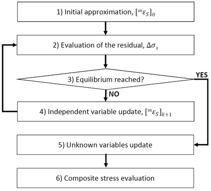
The following organigram (Figure 15) summarizes the steps to be followed in order to give an answer to the problem stated previously. If these steps are included in a FE code as the composite constitutive model [7,8], the code will be suitable for the modelization of LFC problems.

Figure 15: Flow chart with the strategy followed to solve the system of equations

• Initial approximation. An initial value for the variable ${\textstyle {^{m}}{\boldsymbol {\varepsilon }}_{S}}$ is needed. The accuracy of this initial approximation will influence the number of iterations required for the problem convergence. Thus, it is important to provide a good attempt for the first iteration, ${\textstyle \left[{^{m}}{\boldsymbol {\varepsilon }}_{S}\right]_{k=0}}$. This is usually achieved considering a linear behaviour for all the component materials. If the hypothesis is true, the obtained value will be correct and no iterations will be needed. This is expressed as:

$\left[{^{m}}\Delta {\boldsymbol {\sigma }}\right]_{0}={^{t}}\left[{^{m}}\mathbb {C} \right]:\left[{^{m}}\Delta {\boldsymbol {\varepsilon }}\right]_{0}$

(4.26)

$\left[{^{f}}\Delta {\boldsymbol {\sigma }}\right]_{0}={^{t}}\left[{^{f}}\mathbb {C} \right]:\left[{^{f}}\Delta {\boldsymbol {\varepsilon }}\right]_{0}$

(4.27)

Where ${\textstyle \left[{^{i}}\Delta \bullet \right]_{0}={^{t+\Delta t}}\left[{^{i}}\bullet \right]_{0}-{^{t}}\left[{^{i}}\bullet \right]}$ with ${\textstyle i=f}$ or ${\textstyle m}$, is the increment of the variable ${\textstyle \left[{^{i}}\bullet \right]}$ from one step to the next (do not confuse with the residual to be minimized introduced in Equation 4.25), the subscript ${\textstyle 0}$ indicates the first iteration of the new step ${\textstyle t+\Delta t}$ and ${\textstyle {^{t}}\left[{^{i}}\mathbb {C} \right]}$ is the tangent constitutive tensor of each component material ${\textstyle i=f}$ or ${\textstyle m}$, computed using the set of known variables shown in Equation 4.22.

Considering now only the serial terms of the previous expressions, as set in Equation 4.8:

$\left[{^{m}}\Delta {\boldsymbol {\sigma }}_{S}\right]_{0}={^{t}}\left[{^{m}}\mathbb {C} _{SS}\right]:\left[{^{m}}\Delta {\boldsymbol {\varepsilon }}_{S}\right]_{0}+{^{t}}\left[{^{m}}\mathbb {C} _{SP}\right]:\left[{^{m}}\Delta {\boldsymbol {\varepsilon }}_{P}\right]_{0}$

(4.28)

$\left[{^{f}}\Delta {\boldsymbol {\sigma }}_{S}\right]_{0}={^{t}}\left[{^{f}}\mathbb {C} _{SS}\right]:\left[{^{f}}\Delta {\boldsymbol {\varepsilon }}_{S}\right]_{0}+{^{t}}\left[{^{f}}\mathbb {C} _{SP}\right]:\left[{^{f}}\Delta {\boldsymbol {\varepsilon }}_{P}\right]_{0}$

(4.29)

Using these two expressions and the relations set by the Closure Equation 4.20:

$\overbrace {\left[{^{m}}\Delta {\boldsymbol {\sigma }}_{S}\right]_{0}-\left[{^{f}}\Delta {\boldsymbol {\sigma }}_{S}\right]_{0}} ^{=0}={^{t}}\left[{^{m}}\mathbb {C} _{SS}\right]:\left[{^{m}}\Delta {\boldsymbol {\varepsilon }}_{S}\right]_{0}+{^{t}}\left[{^{m}}\mathbb {C} _{SP}\right]:\overbrace {\left[{^{m}}\Delta {\boldsymbol {\varepsilon }}_{P}\right]_{0}} ^{=\left[\Delta {\boldsymbol {\varepsilon }}_{P}\right]_{0}}-$ $-{^{t}}\left[{^{f}}\mathbb {C} _{SS}\right]:\left[{^{f}}\Delta {\boldsymbol {\varepsilon }}_{S}\right]_{0}+{^{t}}\left[{^{f}}\mathbb {C} _{SP}\right]:\overbrace {\left[{^{f}}\Delta {\boldsymbol {\varepsilon }}_{P}\right]_{0}} ^{=\left[\Delta {\boldsymbol {\varepsilon }}_{P}\right]_{0}}\Longrightarrow$

$\Longrightarrow 0={^{t}}\left[{^{m}}\mathbb {C} _{SS}\right]:\left[{^{m}}\Delta {\boldsymbol {\varepsilon }}_{S}\right]_{0}-{^{t}}\left[{^{f}}\mathbb {C} _{SS}\right]:\left[{^{f}}\Delta {\boldsymbol {\varepsilon }}_{S}\right]_{0}+$ $+\left({^{t}}\left[{^{m}}\mathbb {C} _{SP}\right]-{^{t}}\left[{^{f}}\mathbb {C} _{SP}\right]\right):\left[\Delta {\boldsymbol {\varepsilon }}_{P}\right]_{0}$

(4.30)

This equation can be simplified using the Compatibility Conditions (Equation 4.14):

$0={^{t}}\left[{^{m}}\mathbb {C} _{SS}\right]:\left[{^{m}}\Delta {\boldsymbol {\varepsilon }}_{S}\right]_{0}-{^{t}}\left[{^{f}}\mathbb {C} _{SS}\right]:\left({\dfrac {1}{{^{f}}k}}\left[\Delta {\boldsymbol {\varepsilon }}_{S}\right]_{0}-{\dfrac {{^{m}}k}{{^{f}}k}}\left[{^{m}}\Delta {\boldsymbol {\varepsilon }}_{S}\right]_{0}\right)+$ $+\left({^{t}}\left[{^{m}}\mathbb {C} _{SP}\right]-{^{t}}\left[{^{f}}\mathbb {C} _{SP}\right]\right):\left[\Delta {\boldsymbol {\varepsilon }}_{P}\right]_{0}\Longrightarrow$

$\Longrightarrow \left({^{t}}\left[{^{m}}\mathbb {C} _{SS}\right]+{\dfrac {{^{m}}k}{{^{f}}k}}{^{t}}\left[{^{f}}\mathbb {C} _{SS}\right]\right):\left[{^{m}}\Delta {\boldsymbol {\varepsilon }}_{S}\right]_{0}=$ $={\dfrac {1}{{^{f}}k}}{^{t}}\left[{^{f}}\mathbb {C} _{SS}\right]:\left[\Delta {\boldsymbol {\varepsilon }}_{S}\right]_{0}+\left({^{t}}\left[{^{m}}\mathbb {C} _{SP}\right]-{^{t}}\left[{^{f}}\mathbb {C} _{SP}\right]\right):\left[\Delta {\boldsymbol {\varepsilon }}_{P}\right]_{0}$

(4.31)

And finally, setting: ${\textstyle \mathbb {A} =\left({^{f}}k{^{t}}\left[{^{m}}\mathbb {C} _{SS}\right]+{^{m}}k{^{t}}\left[{^{f}}\mathbb {C} _{SS}\right]\right)^{-1}}$, Equation 4.31 is rewritten as:

$\left[{^{m}}\Delta {\boldsymbol {\varepsilon }}_{S}\right]_{0}=\mathbb {A} :\left[{^{t}}\left[{^{f}}\mathbb {C} _{SS}\right]:\left[\Delta {\boldsymbol {\varepsilon }}_{S}\right]_{0}+{^{f}}k\left({^{t}}\left[{^{m}}\mathbb {C} _{SP}\right]-{^{t}}\left[{^{f}}\mathbb {C} _{SP}\right]\right):\left[\Delta {\boldsymbol {\varepsilon }}_{P}\right]_{0}\right]$

(4.32)

From this equation, ${\textstyle {^{t+\Delta t}}\left[{^{m}}{\boldsymbol {\varepsilon }}_{S}\right]_{k=0}}$ is computed (${\textstyle {^{t+\Delta t}}\left[{^{m}}{\boldsymbol {\varepsilon }}_{S}\right]_{k=0}={^{t}}\left[{^{m}}{\boldsymbol {\varepsilon }}_{S}\right]+\left[{^{m}}\Delta {\boldsymbol {\varepsilon }}_{S}\right]_{0}}$) and the algorithm moves to step 2.

• Evaluation of the residual. Once the independent variable ${\textstyle {^{t+\Delta t}}\left[{^{m}}{\boldsymbol {\varepsilon }}_{S}\right]_{k}}$ has been obtained, it is necessary to determine its reliability by means of the residual. It is computed as shown in Equation 4.25, using the serial stress values at ${\textstyle t+\Delta t}$ of each component material. Thus, obtaining ${\textstyle {^{t+\Delta t}}\left[{^{m}}{\boldsymbol {\sigma }}\right]}$ and ${\textstyle {^{t+\Delta t}}\left[{^{f}}{\boldsymbol {\sigma }}\right]}$ is the main objective of this step because Equation 4.7 allows the computation of the serial component of these variables.

The first thing to do before the serial stress imbalance could be estimated, is to determine the total strains for each component:

$\left[{^{m}}{\boldsymbol {\varepsilon }}\right]_{k}=\left[{^{m}}{\boldsymbol {\varepsilon }}_{P}\right]+\left[{^{m}}{\boldsymbol {\varepsilon }}_{S}\right]_{k},{\textrm {where:}}\left[{^{m}}{\boldsymbol {\varepsilon }}_{P}\right]=\left[{^{f}}{\boldsymbol {\varepsilon }}_{P}\right]=\left[{\boldsymbol {\varepsilon }}_{P}\right]$ $\left[{^{f}}{\boldsymbol {\varepsilon }}\right]_{k}=\left[{^{f}}{\boldsymbol {\varepsilon }}_{P}\right]+\left[{^{f}}{\boldsymbol {\varepsilon }}_{S}\right]_{k},{\textrm {where:}}\left[{^{f}}{\boldsymbol {\varepsilon }}_{S}\right]_{k}={\dfrac {1}{{^{f}}k}}\left[{\boldsymbol {\varepsilon }}_{S}\right]-{\dfrac {{^{m}}k}{{^{f}}k}}\left[{^{m}}{\boldsymbol {\varepsilon }}_{S}\right]_{k}$

(4.33)

These equations are based on the complementarity property of the serial and parallel parts of the strain and stress fields (equations 4.10 and 4.11) and are valid for all the iterations of the problem, therefore, ${\textstyle k}$ is not necessary equal to ${\textstyle 0}$.

Finally, the stresses and the internal variables are computed based on the real constitutive model of each component material (the elastic hypothesis used at step 1 is no longer valid) and the residual ${\textstyle \Delta {\boldsymbol {\sigma }}_{S}={^{m}}{\boldsymbol {\sigma }}_{S}-{^{f}}{\boldsymbol {\sigma }}_{S}}$ is evaluated.

• Equilibrium reached?. At this stage, the algorithm decides whether the obtained solution for the set of variables at step ${\textstyle t+\Delta t}$ is valid or not. This decision is made according to a given tolerance. Its value is imposed as a function of the serial stresses for each component at the previous step ${\textstyle t}$, i.e. ${\textstyle tol\sim f\left({^{t}}\left[{^{i}}{\boldsymbol {\sigma }}_{S}\right]\right){\textrm {,where}}i=f,m}$ [8]. This function is defined as:

$f_{1}\left({^{t}}\left[{^{m}}{\boldsymbol {\sigma }}_{S}\right],{^{t}}\left[{^{f}}{\boldsymbol {\sigma }}_{S}\right]\right)=\min \left\lbrace ||{^{t}}\left[{^{m}}{\boldsymbol {\sigma }}_{S}\right]||,||{^{t}}\left[{^{f}}{\boldsymbol {\sigma }}_{S}\right]||\right\rbrace$ $f_{2}\left({^{t}}\left[{^{m}}{\boldsymbol {\sigma }}_{S}\right],{^{t}}\left[{^{f}}{\boldsymbol {\sigma }}_{S}\right]\right)=\min \left\lbrace ||{^{t}}\left[{^{m}}\mathbb {C} _{SS}\right]:\left[{\boldsymbol {\varepsilon }}_{S}\right]||,||{^{t}}\left[{^{f}}\mathbb {C} _{SS}\right]:\left[{\boldsymbol {\varepsilon }}_{S}\right]||\right\rbrace$ $tol=10^{-4}\cdot \left\{{\begin{matrix}&f_{1}\left({^{t}}\left[{^{m}}{\boldsymbol {\sigma }}_{S}\right],{^{t}}\left[{^{f}}{\boldsymbol {\sigma }}_{S}\right]\right),\quad {\textrm {if}}\quad f_{1}\left({^{t}}\left[{^{m}}{\boldsymbol {\sigma }}_{S}\right],{^{t}}\left[{^{f}}{\boldsymbol {\sigma }}_{S}\right]\right)>0\\&f_{2}\left({^{t}}\left[{^{m}}{\boldsymbol {\sigma }}_{S}\right],{^{t}}\left[{^{f}}{\boldsymbol {\sigma }}_{S}\right]\right),\quad {\textrm {if}}\quad f_{1}\left({^{t}}\left[{^{m}}{\boldsymbol {\sigma }}_{S}\right],{^{t}}\left[{^{f}}{\boldsymbol {\sigma }}_{S}\right]\right)=0\end{matrix}}\right.$

(4.34)

Therefore:

${\textrm {If}}\quad ||\left[\Delta {\boldsymbol {\sigma }}_{S}\right]_{k}||\leq tol\quad {\textrm {thengoto''Step5''.}}$ ${\textrm {If}}\quad ||\left[\Delta {\boldsymbol {\sigma }}_{S}\right]_{k}||>tol\quad {\textrm {thengoto''Step4''.}}$

(4.35)

• Independent variable update. This step is used when the ${\textstyle {^{t+\Delta t}}\left[{^{m}}{\boldsymbol {\varepsilon }}_{S}\right]_{k}}$ value is not good enough according to the tolerance computed at step 3. In this case, ${\textstyle {^{t+\Delta t}}\left[{^{m}}{\boldsymbol {\varepsilon }}_{S}\right]_{k}}$ should be recalculated as follows:

• Compute the tangent constitutive tensor for each component material ${\textstyle {^{t+\Delta t}}\left[{^{i}}\mathbb {C} \right]_{k}}$ using the results of the current iteration step k, i.e. ${\textstyle {^{t+\Delta t}}\left[{^{i}}{\boldsymbol {\varepsilon }}\right]_{k}}$ and ${\textstyle {^{t+\Delta t}}\left[{^{i}}{\boldsymbol {\beta }}\right]_{k}}$.

• Jacobian matrix computation [8,7].

${^{t+\Delta t}}\left[\mathbb {J} \right]_{k}={^{t+\Delta t}}\left[{^{m}}\mathbb {C} _{SS}\right]_{k}+{\dfrac {{^{m}}k}{{^{f}}k}}{^{t+\Delta t}}\left[{^{f}}\mathbb {C} _{SS}\right]_{k}$

(4.36)

Where ${\textstyle \left[{^{m}}\mathbb {C} _{SS}\right]}$ and ${\textstyle \left[{^{f}}\mathbb {C} _{SS}\right]}$ are computed as shown in Equation 4.9 from the tangent constitutive tensors ${\textstyle \left[{^{m}}\mathbb {C} \right]}$ and ${\textstyle \left[{^{f}}\mathbb {C} \right]}$. This expression is obtained from the general Jacobian definition introduced in Section 3.3 and using its notation: ${\textstyle \Delta f=\Delta {\boldsymbol {\sigma }}_{S}}$ and ${\textstyle u={^{m}}{\boldsymbol {\varepsilon }}_{S}}$. Therefore:

$\left[\mathbb {J} \right]_{k}=\left.{\dfrac {\partial \left[\Delta {\boldsymbol {\sigma }}_{S}\right]}{\partial \;{^{m}}{\boldsymbol {\varepsilon }}_{S}}}\right|_{{^{m}}{\boldsymbol {\varepsilon }}_{S}=\left[{^{m}}{\boldsymbol {\varepsilon }}_{S}\right]_{k}}={\dfrac {\partial \left[{^{m}}{\boldsymbol {\sigma }}_{S}\right]_{k}}{\partial \;{^{m}}{\boldsymbol {\varepsilon }}_{S}}}-{\dfrac {\partial \left[{^{f}}{\boldsymbol {\sigma }}_{S}\right]_{k}}{\partial \;{^{f}}{\boldsymbol {\varepsilon }}_{S}}}:{\dfrac {\partial \;{^{f}}{\boldsymbol {\varepsilon }}_{S}}{\partial \;{^{m}}{\boldsymbol {\varepsilon }}_{S}}}=$ $=\left[{^{m}}\mathbb {C} _{SS}\right]_{k}-\left[{^{f}}\mathbb {C} _{SS}\right]_{k}:\left(-{\dfrac {{^{m}}k}{{^{f}}k}}\;\mathbb {I} \right)=$ $=\underbrace {\left[{^{m}}\mathbb {C} _{SS}\right]_{k}+{\dfrac {{^{m}}k}{{^{f}}k}}\left[{^{f}}\mathbb {C} _{SS}\right]_{k}} _{Eq.4.36}$

(4.37)

• Unknown ${\textstyle {^{t+\Delta t}}\left[{^{m}}{\boldsymbol {\varepsilon }}_{S}\right]_{k}}$ update. Once more, this is done as previously introduced in Section 3.3:

${^{t+\Delta t}}\left[{^{m}}{\boldsymbol {\varepsilon }}_{S}\right]_{k+1}={^{t+\Delta t}}\left[{^{m}}{\boldsymbol {\varepsilon }}_{S}\right]_{k}-{^{t+\Delta t}}\left[\mathbb {J} \right]_{k}^{-1}:\left[\Delta {\boldsymbol {\sigma }}_{S}\right]_{k}$

(4.38)

Once this has been done, the algorithm moves back to step 2 and starts a new iteration ${\textstyle k+1}$.

• Unknown variables update. Once the problem has converged, it is time to prepare the data for the next time step. The results of the variables stated at Equation 4.24 are now the known variables of the new time step.

• Composite stress evaluation. At this last step the composite total stress (${\textstyle {^{t+\Delta t}}\left[{\boldsymbol {\sigma }}\right]}$) is computed. This is done using the Equation 4.12:

${^{t+\Delta t}}\left[{\boldsymbol {\sigma }}\right]={^{f}}k\,{^{t+\Delta t}}\left[{^{f}}{\boldsymbol {\sigma }}\right]+{^{m}}k\,{^{t+\Delta t}}\left[{^{m}}{\boldsymbol {\sigma }}\right]$

(4.39)

This algorithm is used to obtain the unknowns at all the composite elements of the FE mesh used in the simulation. This provides the local solution of the problem, but the global behaviour is still unknown. The global solution for the structure is obtained through the Equation 3.21, where the global stiffness matrix is made up of all the composite tangent constitutive tensors ${\textstyle \mathbb {C} }$ from each element of the FE mesh. Two approaches can be followed in order to obtain these tensors:

• Calculation using numerical perturbations [37]. At this stage, the stress and strain fields of the composite material are known, therefore the composite ${\textstyle \mathbb {C} }$ tensor can be obtained activating small strains and analysing the results obtained, i.e. ${\textstyle \mathbb {C} ={\boldsymbol {\sigma }}:{\boldsymbol {\varepsilon }}^{-1}}$.

• Calculation through the component tangent constitutive tensors [8,9]. The composite tangent constitutive tensor has been defined in Equations 4.8 and 4.9. These expressions can be written in terms of the components tangent constitutive tensors as:

$\mathbb {C} _{PP}={^{m}}k{^{f}}k\left({^{f}}\mathbb {C} _{PS}-{^{m}}\mathbb {C} _{PS}\right):\mathbb {A} :\left({^{f}}\mathbb {C} _{SP}-{^{m}}\mathbb {C} _{SP}\right)+$ $+\left({^{f}}k{^{f}}\mathbb {C} _{PP}+{^{m}}k{^{m}}\mathbb {C} _{PP}\right)$ $\mathbb {C} _{PS}=\left({^{f}}k{^{f}}\mathbb {C} _{PS}:\mathbb {A} :{^{m}}\mathbb {C} _{SS}+{^{m}}k{^{m}}\mathbb {C} _{PS}:\mathbb {A} :{^{f}}\mathbb {C} _{SS}\right)$ $\mathbb {C} _{SP}=\left({^{m}}k{^{f}}\mathbb {C} _{SS}:\mathbb {A} :{^{m}}\mathbb {C} _{SP}+{^{f}}k{^{m}}\mathbb {C} _{SS}:\mathbb {A} :{^{f}}\mathbb {C} _{SP}\right)$ $\mathbb {C} _{SS}={\dfrac {1}{2}}\left[\left({^{m}}\mathbb {C} _{SS}:\mathbb {A} :{^{f}}\mathbb {C} _{SS}\right)+\left({^{f}}\mathbb {C} _{SS}:\mathbb {A} :{^{m}}\mathbb {C} _{SS}\right)\right]$

(4.40)

By doing this, it is possible now to solve the global system of equations and move to the next time step.

4.3 Prestressed concrete structures singularities

At this stage, the general algorithm used for the SP RoM and all the properties of the LFCs are known. Despite this, as the present monograph is focused on the analysis of prestressed concrete structures, some of the introduced generalities can be particularized.

Constitutive models

The main advantage of the SP RoM is the chance to use whatever constitutive model is desired for the component materials. This allows to capture perfectly the behaviour of simple materials and then the algorithm will automatically compute the complex response of the composite material. Thus, it is interesting to know which are the constitutive models selected for the prestressed concrete analysis driven in this project.

Concrete modelization - Isotropic continuous damage model

The Continuum Damage Mechanics is a branch of the Continuum Mechanics that provides the needed framework for characterizing, representing and modelling the effects of distributed defects on the material behaviour. The propagation and coalescence of these defects generates a progressive and irreversible degradation of the elastic properties of the material, characterized by a stiffness loss [30,39,32].

The Continuous Damage theory was first introduced by Kachanov [40] in 1958 but it has evolved from then and now there are several approaches that can be used in the damage field. For the purpose of this monograph, the isotropic continuous damage model has been chosen for the concrete modelization. During the last years the use of this constitutive model has been widely accepted for the simulation of many materials used in engineering [41,42] due to its simplicity in the implementation, versatility and coherence.

The isotropic damage model is completely characterized by one variable (${\textstyle d}$) that takes into account the presence and growth of small fractures and micro voids in the material structure. Thus, this damage variable measures the level of deterioration in the material and works affecting the stress field by transforming the stress real tensor into an effective stress tensor. In general terms, this is expressed as:

${\boldsymbol {\sigma }}_{0}=\mathbb {M} ^{-1}:{\boldsymbol {\sigma }}$

(4.41)

Where ${\textstyle \mathbb {M} }$ is the fourth-order tensor of the anisotropic damage model. Nevertheless, for the isotropic damage model that has been used for concrete, the tensor only depends on one scalar variable ${\textstyle d}$ and Equation 4.41 can be rewritten as:

${\boldsymbol {\sigma }}_{0}=\left[\left(1-d\right)\mathbb {I} \right]^{-1}:{\boldsymbol {\sigma }}={\dfrac {\boldsymbol {\sigma }}{1-d}}{\textrm {,}}d\in \left[0,1\right]$

(4.42)

Where ${\textstyle {\boldsymbol {\sigma }}}$ is the Cauchy stress tensor, ${\textstyle {\boldsymbol {\sigma }}_{0}}$ is the effective stress tensor and ${\textstyle d}$ is the internal variable of damage such that ${\textstyle d=0}$ indicates that the material is not damaged and ${\textstyle d=1}$ indicates that the material is completely damaged, i.e. there is a local fracture.

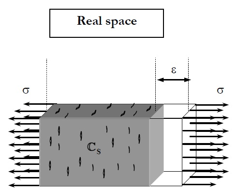
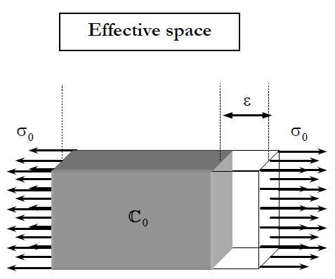
The effective stress ${\textstyle {\boldsymbol {\sigma }}_{0}}$ concept was first introduced by Kachanov (1958) to carry out fracture simulations. This tensor must be understood as the stress state in a non-damaged element, which generates the same strain that ${\textstyle {\boldsymbol {\sigma }}}$ produces in a damaged element. Figure 16 represents this idea.

(a) Damaged real element	(b) Non-damaged equivalent element
Figure 16: Graphic representation of the effective stress definition [32]

Consequently, the relation between ${\textstyle {\boldsymbol {\sigma }}_{0}}$ and the induced strain (${\textstyle {\boldsymbol {\varepsilon }}}$) can be formulated in elastic terms as:

${\boldsymbol {\sigma }}_{0}=\mathbf {C} \,{\boldsymbol {\varepsilon }}$

(4.43)

Where ${\textstyle \mathbf {C} }$ is the elastic constitutive matrix. Considering now the formulation in terms of the real stress tensor ${\textstyle {\boldsymbol {\sigma }}}$ by using Equation 4.42, the constitutive law for the isotropic damage model can be written as:

${\boldsymbol {\sigma }}=\left(1-d\right)\mathbf {C} \,{\boldsymbol {\varepsilon }}$

(4.44)

Now, only one question remains: How is the internal variable of damage ${\textstyle d}$ controlled? Of course ${\textstyle d}$ is not constant. It is defined by two properties:

• Damage threshold criterion. This makes the distinction between an elastic behaviour of the material and another in which the degradation process of the material's properties takes place. This criterion is specific to the material that is being modelled but can be defined in general terms as:

$\mathbb {F} \left({\boldsymbol {\sigma }}_{0};\mathbf {q} \right)=f\left({\boldsymbol {\sigma }}_{0}\right)-c\left(d\right)\leq 0,\quad \mathrm {with} \;q\equiv \left\lbrace d\right\rbrace$

(4.45)

Where ${\textstyle f\left({\boldsymbol {\sigma }}_{0}\right)}$ is a function of the stress tensor ${\textstyle {\boldsymbol {\sigma }}_{0}=\mathbb {C} _{0}:{\boldsymbol {\varepsilon }}}$ and ${\textstyle c\left(d\right)}$ is the scalar function defining the damage threshold position. The initial value of this damage threshold ${\textstyle c\left(d^{0}\right)=c^{max}={\boldsymbol {\sigma }}^{max}}$ is a property of the material and is related to its compressive strength.

Concrete is the material that is being simulated using the damage model, therefore a yield criteria appropriate for frictional materials is needed. The FE code used during the analysis performed for this monograph uses the Mohr-Coulomb modified function [32]. This yield criteria is specific for concrete, which has an internal friction angle of ${\textstyle \phi =32^{\circ }}$ and a compression - tension strength ratio ${\textstyle \mathbb {R} _{Mohr}^{0}=\|{\boldsymbol {\sigma }}_{C}^{0}/{\boldsymbol {\sigma }}_{T}^{0}\|\simeq 10.0}$. These characteristics cannot be achieved with the original Mohr-Coulomb function and so this alternative is used. In this scenario, Equation 4.45 is rewritten as:

${\begin{matrix}\mathbb {F} \left({\boldsymbol {\sigma }},c,\phi \right)=f\left({\boldsymbol {\sigma }},\phi \right)-c\left(d\right)=0\\\mathrm {or} \\{\bar {\mathbb {F} }}\left({\boldsymbol {\sigma }},c,\phi \right)=G\left[f\left({\boldsymbol {\sigma }},\phi \right)\right]-G\left[c\left(d\right)\right]=0\end{matrix}}$

(4.46)

Both expressions are equivalent. ${\textstyle G\left[\chi \right]}$ is a scalar monotonically increasing function, positive invertible, with positive derivative, ${\textstyle f\left({\boldsymbol {\sigma }},\phi \right)}$ is the stress function that control the Mohr-Coulomb function, which can be expressed as:

$f\left({\boldsymbol {\sigma }},\phi \right)={\dfrac {1}{\cos \left(\phi \right)}}\left\lbrace {\dfrac {I_{1}}{3}}\mathbb {K} _{3}+{\sqrt {J_{2}}}\left[\mathbb {K} _{1}\cos \left(\theta \right)-\mathbb {K} _{2}{\dfrac {\sin \left(\theta \right)\sin \left(\phi \right)}{\sqrt {3}}}\right]\right\rbrace$

(4.47)

${\textstyle I_{1}}$ is the first invariant of the stress tensor, ${\textstyle J_{2}}$ is the second invariant of the deviatoric stress tensor and ${\textstyle \theta }$ is the Lode's similarity angle ${\textstyle \theta =\arcsin \left[\left(3{\sqrt {3}}J_{3}\right)/\left(2J_{2}^{3/2}\right)\right]}$. ${\textstyle \mathbb {K} _{i}}$ are the factors that allow the generalisation of the Mohr-Coulomb yield function and thus, depend on the friction angle ${\textstyle \phi }$ and on the compression - tension ratio.

]

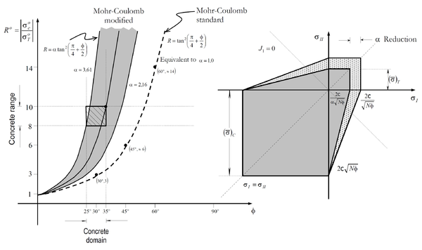Figure 17: Graphical representation of the Mohr-Coulomb modified function [32]

• Evolution law of the damage variable, ${\textstyle d}$. The general equation that determines the evolution of this variable is:

${\dot {d}}={\dot {\mu }}{\dfrac {\partial {\bar {\mathbb {F} }}\left({\boldsymbol {\sigma }}_{0};\mathbf {q} \right)}{\partial \left[f\left({\boldsymbol {\sigma }}_{0}\right)\right]}}\equiv {\dot {\mu }}{\dfrac {\partial G\left[f\left({\boldsymbol {\sigma }}_{0}\right)\right]}{\partial \left[f\left({\boldsymbol {\sigma }}_{0}\right)\right]}}$

(4.48)

Where ${\textstyle \mu }$ is a non-negative scalar called damage consistency parameter, which is used to define loading, unloading and reloading conditions [32].

Therefore, the damage criterion can change depending on the definition of the ${\textstyle G\left[\chi \right]}$ functions, which control the threshold and the evolution of the damage law.

The damage model used for the concrete modelization in this monograph is based on an exponential approach, which leads to the following expression for the damage internal variable:

$d=1-\left[{\dfrac {f^{0}\left({\boldsymbol {\sigma }}_{0}\right)}{\tau }}e^{A\left(1-{\dfrac {\tau }{f^{0}\left({\boldsymbol {\sigma }}_{0}\right)}}\right)}\right]$

(4.49)

Where ${\textstyle f^{0}\left({\boldsymbol {\sigma }}_{0}\right)=c^{max}}$ is the initial value of the damage threshold, ${\textstyle A}$ is a parameter that depends on the fracture energy and ${\textstyle \tau }$ is the damage threshold condition, which sets the beginning of the damage procedure for ${\textstyle \tau =G\left[f\left({\boldsymbol {\sigma }}_{0}\right)\right]>\tau _{max}=G\left[c\left(d\right)\right]}$.

Finally, the effect of the damage in the material is, of course, a progressive degradation of the material properties. This means that the constitutive matrix ${\textstyle \mathbb {C} }$ is not constant and so it is necessary to define it in terms of the damage parameters and compute it at each iteration and time step. This is the tangent constitutive tensor of damage:

$\mathbb {C} ^{T}=\left(1-d\right)\mathbb {C} _{0}-{\dfrac {\partial G\left[f\left({\boldsymbol {\sigma }}_{0}\right)\right]}{\partial \left[f\left({\boldsymbol {\sigma }}_{0}\right)\right]}}\left[\mathbb {C} _{0}:{\boldsymbol {\varepsilon }}\right]\otimes {\dfrac {\partial f\left(\mathbb {C} _{0}:{\boldsymbol {\varepsilon }}\right)}{\partial {\boldsymbol {\varepsilon }}}}$

(4.50)

Using all this information, the constitutive model used for the concrete is completely defined.

Prestressing steel modelization - Viscoelasticity model

Prestressing steel is characterized by a high compressive/tensile strength compared to the other component materials of the prestressed concrete. This allows considering an elastic constitutive model for its numerical modelization. Despite this, the use of a constitutive model constant in time does not reproduce the real behaviour of this material. A time-dependent model is needed instead.

There are two types of time-dependent elasticity models [32]:

• Delayed elasticity or creep model. In these models, the stress is the free variable of the problem and so the strains change in time depending on the free variable value. The Kelvin viscoelastic model is a good example. This idea is shown in Figure 18a.
• Relaxation model. In these models the strain is the free variable of the problem and so the stresses change in time depending on the free variable value. The Maxwell viscoelastic model is a good example. This idea is shown in Figure 18b.

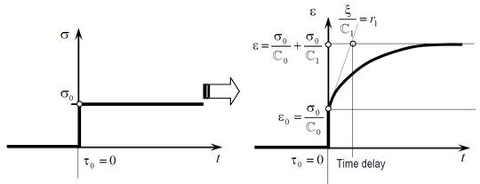
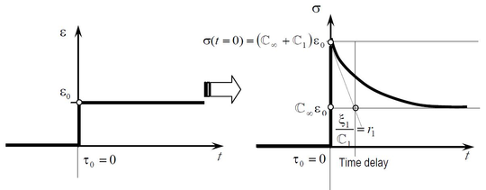
(a) Response of the generalized Kelvin model under a constant stress	(b) Response of the generalized Maxwell model under a constant deformation
Figure 18: Time-dependent elasticity models [32]

The prestressing steel behaviour in time consists of a progressive stress loss and thus, the Maxwell model is the one chosen for the material modelization. In fact, a generalization of this model is used: the generalized Maxwell model.

Before moving to the multiaxial generalization of this model, it is better to introduce it using an uniaxial representation based on a spring-damping analogy (Figure 19).

]

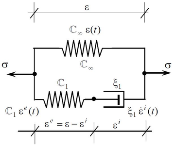Figure 19: The Generalized Maxwell model [32]

In this model, the stress state at any time is expressed in terms of the free variable ${\textstyle {\boldsymbol {\varepsilon }}}$ as:

${\boldsymbol {\sigma }}\left(t\right)={\boldsymbol {\sigma }}^{i}\left(t\right)+{\boldsymbol {\sigma }}^{\infty }\left(t\right),\quad \mathrm {where:} \left\{{\begin{matrix}&{\boldsymbol {\sigma }}^{i}\left(t\right)=\mathbb {C} _{1}\left({\boldsymbol {\varepsilon }}\left(t\right)-{\boldsymbol {\varepsilon }}^{i}\left(t\right)\right)=\xi _{1}{\dot {\boldsymbol {\varepsilon }}}^{i}\left(t\right)\\&{\boldsymbol {\sigma }}^{\infty }\left(t\right)=\mathbb {C} _{\infty }{\boldsymbol {\varepsilon }}\left(t\right)\end{matrix}}\right.$

(4.51)

This equation expresses mathematically what is shown in Figure 19: the model is governed by an elastic component and an inelastic component. The inelastic component progressively disappears with time until the elastic component fully controls the material behaviour.

Adding both terms in Equation 4.51 the equilibrium condition is written:

${\boldsymbol {\sigma }}\left(t\right)={\boldsymbol {\sigma }}^{i}\left(t\right)+{\boldsymbol {\sigma }}^{\infty }\left(t\right)=\mathbb {C} _{1}\left({\boldsymbol {\varepsilon }}\left(t\right)-{\boldsymbol {\varepsilon }}^{i}\left(t\right)\right)+\mathbb {C} _{\infty }{\boldsymbol {\varepsilon }}\left(t\right)=\xi _{1}{\dot {\boldsymbol {\varepsilon }}}^{i}\left(t\right)+\mathbb {C} _{\infty }{\boldsymbol {\varepsilon }}\left(t\right)$

(4.52)

This can also be expressed as:

${\boldsymbol {\sigma }}\left(t\right)=\mathbb {C} _{0}{\boldsymbol {\varepsilon }}\left(t\right)-\mathbb {C} _{1}{\boldsymbol {\varepsilon }}^{i}$

(4.53)

Where ${\textstyle \mathbb {C} _{0}=\mathbb {C} _{\infty }+\mathbb {C} _{1}}$.

These equations fully define the Maxwell model, they are the constitutive equation. Despite this, it is interesting to eliminate the inelastic strain variable from the equation. This can be achieved by solving the differential equation:

${\dfrac {{\boldsymbol {\varepsilon }}\left(t\right)}{r_{1}}}={\dfrac {{\boldsymbol {\varepsilon }}^{i}\left(t\right)}{r_{1}}}+{\dot {\boldsymbol {\varepsilon }}}^{i}\left(t\right)$

(4.54)

Where ${\textstyle r_{1}={\dfrac {\xi _{1}}{\mathbb {C} _{1}}}}$. This equation is obtained from the definition of the inelastic stress component written in Equation 4.51.

The solution of this differential equation is:

$\left\{{\begin{matrix}&{\boldsymbol {\varepsilon }}^{i}\left(t\right)=0\qquad &\forall \,\tau <\tau _{0}\\&{\boldsymbol {\varepsilon }}^{i}\left(t\right)=\int _{-\infty }^{t}{\dfrac {1}{r_{1}}}e^{-\left(t-s\right)/r_{1}}{\boldsymbol {\varepsilon }}\left(s\right)ds\qquad &\forall \,\tau \geq \tau _{0}\end{matrix}}\right.$

(4.55)

Where ${\textstyle \tau _{0}}$ is the time at which a strain ${\textstyle {\boldsymbol {\varepsilon }}\left(t\right)}$ is applied. Substituting this equation into Equation 4.53:

$\left\{{\begin{matrix}&{\boldsymbol {\sigma }}\left(t\right)=0\qquad &\forall \,\tau <\tau _{0}\\&{\boldsymbol {\sigma }}\left(t\right)=\mathbb {C} _{0}{\boldsymbol {\varepsilon }}\left(t\right)-{\dfrac {\mathbb {C} _{0}}{r_{1}}}\int _{-\infty }^{t}e^{-\left(t-s\right)/r_{1}}{\boldsymbol {\varepsilon }}\left(s\right)ds\qquad &\forall \,\tau \geq \tau _{0}\end{matrix}}\right.$

(4.56)

Figure 18b shows the particular case where the imposed strain at time ${\textstyle t=\tau _{0}}$ is:

$\left\{{\begin{matrix}&{\boldsymbol {\varepsilon }}\left(t\right)=0\qquad &\forall \,t<\tau _{0}=0\\&{\boldsymbol {\varepsilon }}\left(t\right)={\boldsymbol {\varepsilon }}_{0}\qquad &\forall \,t\geq \tau _{0}=0\end{matrix}}\right.$

(4.57)

And thus, the stress expression obtained from Equation 4.56:

$\left\{{\begin{matrix}&{\boldsymbol {\sigma }}\left(t\right)=0\qquad &\forall \,\tau <\tau _{0}\\&{\boldsymbol {\sigma }}\left(t\right)=\left(\mathbb {C} _{\infty }+\mathbb {C} _{1}e^{-t/r_{1}}\right){\boldsymbol {\varepsilon }}_{0}\qquad &\forall \,\tau \geq \tau _{0}\end{matrix}}\right.$

(4.58)

Now that the uniaxial approach has been introduced, it is easier to describe the multiaxial approach of the generalized Maxwell model. Equation 4.56 is now written at a time ${\textstyle t+\Delta t}$, as follows:

${\boldsymbol {\sigma }}_{ij}\left(t+\Delta t\right)=\mathbb {C} _{ijkl}\left[{\boldsymbol {\varepsilon }}_{ij}\left(t+\Delta t\right)-{\dfrac {\mathbb {C} _{1}}{\mathbb {C} _{0}\xi }}\int _{-\infty }^{t+\Delta t}e^{-\left(t+\Delta t-s\right)/r_{1}}{\boldsymbol {\varepsilon }}_{kl}\left(s\right)ds\right]=$ $=\mathbb {C} _{ijkl}{\boldsymbol {\varepsilon }}_{ij}\left(t+\Delta t\right)-\left[\mathbb {C} _{ijkl}{\dfrac {\mathbb {C} _{1}}{\mathbb {C} _{0}\xi }}\int _{-\infty }^{t}e^{-\left(t-s\right)/r_{1}}{\boldsymbol {\varepsilon }}_{kl}\left(s\right)\right]-$ $-\mathbb {C} _{ijkl}{\dfrac {\mathbb {C} _{1}}{\mathbb {C} _{0}\xi }}\int _{t}^{t+\Delta t}e^{-\left(t+\Delta t-s\right)/r_{1}}{\boldsymbol {\varepsilon }}_{kl}\left(s\right)=$ $={\boldsymbol {\sigma }}_{ij}\left(t+\Delta t\right)={\boldsymbol {\sigma }}_{ij}\left(t\right)e^{-\left(\Delta t\right)/r_{1}}-\mathbb {C} _{ijkl}{\boldsymbol {\varepsilon }}_{kl}\left(t\right)e^{-\left(\Delta t\right)/r_{1}}\left[1+{\dfrac {\mathbb {C} _{1}}{\mathbb {C} _{0}\xi }}{\dfrac {\Delta t}{2}}\right]+$ $+\mathbb {C} _{ijkl}{\boldsymbol {\varepsilon }}_{kl}\left(t+\Delta t\right)\left[1-{\dfrac {\mathbb {C} _{1}}{\mathbb {C} _{0}\xi }}{\dfrac {\Delta t}{2}}\right]$

(4.59)

Where the integral has been solved using the trapezoidal rule as proposed by Oller (2014) [32].

Effect of the prestressing over the SP RoM formulation

Having a look at the compatibility conditions written in Section 4.2, it can be observed that the current definition of the SP RoM is not valid for the modelization of prestressing steel. Condition 4 imposes that there is no possible relative displacement between component materials, but the prestressing effect imposes an initial relative displacement between the matrix and the fibre. Therefore, it is necessary to modify the original formulation.

A new compatibility condition is included:

• Relative movement between the component materials is allowed if and only if an imposed strain condition exists over one of them.

Therefore, loss of adherence is allowed only in the presence of the prestressing effect, included as an imposed strain.

Equation 4.13 must be modified to take into account the imposition of an initial strain for the fibre in order to represent the prestressing effect. The new equation is piecewise function:

• In the first iteration of the S-P RoM algorithm, the parallel component of the strain tensor of the prestressing steel is fixed to the imposed prestressing value ${\textstyle {\boldsymbol {\varepsilon }}_{imp}}$ and the parallel component of the matrix component remains equal to the parallel component of the composite strain.

${\textrm {incr.}}=1{\textrm {anditer.}}=1\quad \Rightarrow \quad {^{m}}{\boldsymbol {\varepsilon }}_{P}={^{c}}{\boldsymbol {\varepsilon }}_{P}\quad \wedge \quad {^{f}}{\boldsymbol {\varepsilon }}_{P}={\boldsymbol {\varepsilon }}_{imp}$

(4.60)

• For the rest of the steps of the analysis, the parallel component of the strain tensor of the active steel is computed through the current prestressing value ${\textstyle {\boldsymbol {\varepsilon }}_{imp,t}}$ and the parallel component of the composite strain. On the other hand, the parallel component of the matrix component is still equal to the parallel component of the composite strain.

${\textrm {incr.}}\geq 1{\textrm {anditer.}}>1\quad \Rightarrow \quad {^{m}}{\boldsymbol {\varepsilon }}_{P}={^{c}}{\boldsymbol {\varepsilon }}_{P}\quad \wedge \quad {^{f}}{\boldsymbol {\varepsilon }}_{P}={^{c}}{\boldsymbol {\varepsilon }}_{P}+{\boldsymbol {\varepsilon }}_{imp,t}$

(4.61)

Pre/Post tensioned structures and bonding effect

The present monograph is focused on the analysis of post-tensioned concrete structures. Despite this, there are another type of prestressed concrete structures that can be analysed through the SP RoM, i.e. the pre-tensioned concrete structures.

The analysis of these structures do not add any difference to the approach, although the construction procedures and the uses of this typology are different to the ones of post-tensioned structure.

Despite this, there is a specific case in which some modifications must be considered: unbonded post-tensioned concrete structures. In this case, the post-tensioning of steel is modelled by considering the three transversal modulus of the steel close to 0 and therefore allowing the steel to glide without friction inside the concrete. In order to fully allow deformation of the steel in a decoupled way from the concrete, its Poisson coefficients are set to 0, which allows the complete description of the post-tensioning process. Pre-tensioning and bonded post-tensioning, on the other hand, are reproduced by considering both, the transversal modulus and the Poisson coefficients for steel at their common value.

Reinforcing steel

The SP RoM is a useful technique but it has to be used appropriately. The formulation introduced in Section 4.2 is valid for composite materials with only two phases. Therefore, in those cases where a FE contains concrete, prestressing steel and reinforcement steel, the formulation is no longer valid.

The possibility of generalising the SP RoM theory for ${\textstyle n}$ materials exists but it has a big computational cost. A different approach is considered instead.

In general, reinforcing steel has either a clear directional contribution when only longitudinal or transversal reinforcement is used or a uniform effect when it is organized as a dense grid. This allows accounting for it by using an approach introduced in Section 2.2: smeared elements.

Therefore, what is done is that the rebars effect is included in the computation as an increment in the concrete strength. This approach allows the inclusion of different reinforcing contributions in each direction and in each FE.

Finally, by using this methodology the SP RoM formulation is valid again. The two component materials are now: the prestressing steel (${\textstyle =}$ fibre) and the concrete including the rebars contribution (${\textstyle =}$ matrix).

5 Application examples

Once the fundamentals that support the SP RoM theory and the FEM have been introduced, it is time to show how these bases are applied to the analysis of post-tensioned structures.

In this section three cases are presented which are intended to validate the methodology and demonstrate its potential. Two isostatic beams have been selected in order to compare the results obtained with the SP RoM approach and those obtained from an analytical approach.

The last example is the result of the recent work developed at the International Centre for Numerical Method in Engineering (CIMNE). It is the study of a mock-up of a reactor containment building as part of the VeRCoRs Project [43]. This analysis allows to demonstrate the potential of the proposed methodology.

5.1 Required software

The analysis performed has been possible thanks to GiD${\textstyle ^{\mbox{®}}}$ [44,31] and PLastic Crack dynamic (PLCd) [45].

GiD is a pre and post processor for numerical simulations in science and engineering developed by CIMNE. Gid version 13.1.7 has been used for building the models and for the results display. Therefore, the images presented in this section have been obtained with this software.

On the other hand, PLCd is an implicit finite element code for the numerical simulation of nonlinear dynamic behaviour of structures of complex constitution. It was created in 1989 and it has been continuously evolving since then. The SP RoM is implemented in this code, thus it has been used for the calculation of the structures tested here.

Next section will show how these software are used in the calculation procedure.

(a) GiD logo	(b) PLCd logo
Figure 20: Software used during the analysis

5.2 Procedure description

The steps followed during the analysis performed are quite standardized, regardless of what structure is being studied. Thus, it is possible to describe the general procedure and it will remain valid for any case:

• Model generation. The procedure starts creating a 3-D model that represents adequately the structure that is being analysed. It can be generated using GiD preprocessing tools but other software can be used instead and then load it into GiD, which accepts many formats, e.g. IGES, STEP, DXF, ACIS, VDA, Rhinoceros, etc.

The model is complete when all the elements are defined, i.e. lines, surfaces and volumes. Prestressing steel is not included as a 3-D element, curvilinear lines are used with this purpose and, when the SP RoM is performed, the tendon area is taken into account.

• Attributes allocation. Once the model has been created, it is time to define the boundary conditions, the material properties and the load cases and apply them properly to the model entities.

The prestressing force is not assigned at this step. In fact it is defined as an imposed strain and not as a force.

• FE mesh generation. Two FE meshes are generated for the calculations. The first one is built using 8-noded linear hexahedral elements with GiD. It can be structured, unstructured or semistructured depending on the geometry requirements. The second mesh is generated using the tendons. Thus, the other elements are disabled and only the lines that constitute the tendons are used.

• Intersections. This step is used to define the relation between the two meshes, i.e. identify the path that the tendons describe through the hexaedra.

By doing this, besides finding out the hexaedras that are crossed by a tendon, the points where the intersection is produced are found and stored. This operation is essential for the composite material description because these coordinates describe the fibre orientation for each composite material.

• Composite generation. Each composite material is characterized by the matrix and fibre material properties defined and assigned at step 2 and the fibre orientation defined at step 4. With this information, the program compiles all the information and generates a file with all the casuistic and the FEs associated to each one. Thus, this file contains the information that characterize a composite material, i.e. ${\textstyle \mathbf {e} _{1}}$ vector and ${\textstyle {^{f}}k}$ and ${\textstyle {^{m}}k}$ coefficients (see Section 4).

• Description of the loading sequence. The output obtained at the last step is the file required for the PLCd calculation. Despite this, the file is incomplete at this stage. The information missing is the one that describes the load sequences that take place at the structure, the so called stages. At least two stages are usually included: the self-weight and the prestressing operation. These sections include not only the load values and the elements affected by them, but also the increments in which loads are applied or the tolerance admitted at each iteration.

At this moment, the code allows imposing only a constant strain value for each tendon that accounts for the prestressing effect. This means that immediate prestressing losses are not being considered by the software. Therefore, a previous calculation that takes into consideration these losses is necessary and then a mean strain can be used as the initial prestressing value. The procedure followed is explained in detail in Section 5.4.

• Structure computation. PLCd is used now for the computation. The SP RoM approach is applied and the analysis is performed.

• Display of results. The results obtained with PLCd can now be displayed using GiD. The calculation software computes stresses, strains, displacements and reactions, which can be loaded on the structure model and visualized in the post-process.

5.3 Validation examples

Two beams are analysed in this section and two approaches are used in each case: the SP RoM and the analytic formulation used in the Strength of Materials theory [46]. This allows the comparison of the results and the validation of the proposed methodology before moving to a real scenario.

These examples have been faced assuming several simplifications, which allow delimiting the scope of the problem and orient it towards the desired direction:

• Prestressed cantilever with a linear centred tendon. This case has been generated to measure the deformation that a tendon induces in a structural element due to the prestressing effect when it is introduced by one end. The pure longitudinal response can only be achieved when the self weight is not considered and the tendon is linear and is centred in the beam section. Furthermore, as PLCd only admits constant stress distribution at the tendon, the analytic approach must be formulated under the same conditions.

• Prestressed simply supported beam with a parabolic tendon. This example is used to compute the vertical deformation induced by the prestressing force. Again, the self-weight is not considered because it would interfere in the calculations. In addition, a constant stress distribution at the tendon is considered once more.

In both cases elastic materials have been used because the analytic formulation used for comparison works in the elastic domain. Therefore, these are not realistic structures and the results obtained here are not translatable to a real situation, but this is not the purpose of them. They are only used for validating the methodology.

Prestressed cantilever with a linear centred tendon

A cantilever beam has been modelled using GiD (Figure 21). It has a square section with sides ${\textstyle b=h=1.1m}$ and length ${\textstyle L=7m}$. The boundary condition has been imposed on one face by blocking displacements in the three directions (Figure 22).

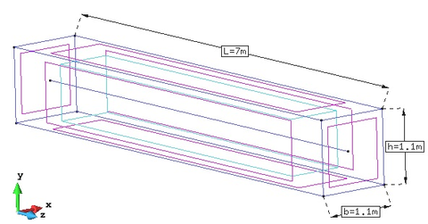
Figure 21: GiD model with the main geometry dimensions

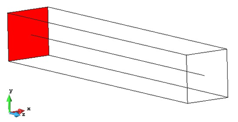
Figure 22: Fixed end of the cantilever beam at GiD model

The properties of the materials used for the beam simulation are summarized in Table 2. These values are frequent for materials used in prestressed structures.

Table. 2 Concrete and prestressing steel properties

Material Properties
Concrete
	Young modulus, $E_{c}$ [GPa]	35.00
	Area, $A_{c}$ [$m^{2}$]	1.205
Prestressing steel
	Young modulus, $E_{p}$ [GPa]	190.00
	Area, $A_{p}$ [$m^{2}$]	0.005
	Prestressing tension [MPa]	1500.00

The material strengths have not been included in the table, this is because, as stated before, the materials are assumed to have an elastic behaviour and so, these parameters are not needed for the current analysis.

Figure 23 shows the FE mesh generated with GiD and needed for the numerical analysis with PLCd. It is composed of 8470 8-nodded hexahedra.

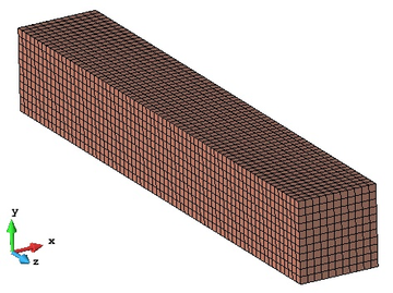
Figure 23: FE mesh created with GiD

The results of the PLCd calculation by means of the SP RoM are shown in Figure 24. The maximum displacement is produced near the free end and is ${\textstyle -1.59\times 10^{-3}m}$. It is located near the end of tendon, but not at the beam surface where the maximum displacement value is ${\textstyle -1.36\times 10^{-3}m}$.

Figure 24: Displacements in z direction [$m$]

For the beam analysis using the Strength of Materials theory, the prestressing effect is transformed into an axial distributed compression load along the whole beam, ${\textstyle N(z)}$ (Figure 25):

$N(z)=\sigma \cdot A_{p}=1500{\textrm {''MPa''}}\cdot 0.005m^{2}=-7500{\textrm {''kN''}}$

(5.1)

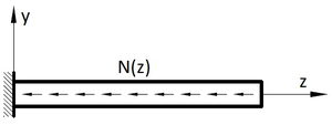
Figure 25: Scheme for the analysis through the Strength of Materials theory

Therefore, the beam total deformation can be written as [46]:

$\delta _{long}=\int _{0}^{L}{\dfrac {N(z)}{E_{comp}A_{comp}}}dz={\dfrac {NL}{E_{c}A_{c}+E_{p}A_{p}}}=$ $=-{\dfrac {7500{\textrm {''kN''}}\cdot 7m}{35{\textrm {''GPa''}}\cdot 1.205m^{2}+190{\textrm {''GPa''}}\cdot 0.005m^{2}}}=-1.22\times 10^{-3}m$

(5.2)

Where ${\textstyle E_{comp}}$ and ${\textstyle A_{comp}}$ are the equivalent Young modulus for the composite material and the section area of the beam. The decomposition into the component variables ${\textstyle E_{c}}$, ${\textstyle E_{p}}$, ${\textstyle A_{c}}$ and ${\textstyle A_{p}}$ only is valid for a full parallel behaviour.

The results obtained with both approaches are similar but the numerical simulation predicts a higher deformation. This happens because, in the analytical calculation, the whole section is supposed to deform equally. This is equivalent to the use of one FE in the whole section and solving the problem through the SP RoM. Nevertheless, this behaviour is not real and what happens in fact is that the area surrounding the tendon deforms more than the external regions, which is the behaviour obtained with the numerical simulation. Thus, the only way to obtain the same results with both approaches would be increasing the prestressing steel area by incrementing the tendon diameter or by adding more tendons.

Figure 26 shows the results of a beam with the same properties as the studied one but with the prestressing effect distributed in more tendons. This test has been performed to demonstrate that the difference between the numerical and the analytical approaches are those stated previously. It can be observed that the obtained deformation for this case with four tendons is almost the same as the one obtained in Equation 5.2.

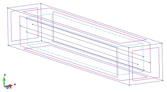
Figure 26: Beam with four prestressed tendons. Model (top) and displacement field in $z$ direction [$m$] (bottom). Prestressing tension: $375$MPa

Prestressed simply supported beam with a parabolic tendon

In this case, a simply supported beam with an embedded parabolic steel tendon has been analysed (Figure 27). It has a square section with sides ${\textstyle b=h=1m}$ and the span between the supports is ${\textstyle L=10m}$. One end of the beam is fully constrained in the three directions, but the other one allows deformations in the horizontal direction. The tendon describes a perfect parabola with eccentricities ${\textstyle e_{1}=e_{2}=0.3m}$ with respect to the beam neutral axis (Figure 31).

Figure 27: GiD model with the main geometry dimensions

The properties of the materials used for the beam simulation are summarized in Table 3. Both tendon ends are active and the prestressing tension is equivalent to a force ${\textstyle P=5000}$kN, that is assumed to be distributed uniformly in the whole length of the tendon.

Table. 3 Concrete and prestressing steel properties

Material Properties
Concrete
	Young modulus, $E_{c}$ [GPa]	35.00
	Area, $A_{c}$ [$m^{2}$]	0.995
Prestressing steel
	Young modulus, $E_{p}$ [GPa]	210.00
	Area, $A_{p}$ [$m^{2}$]	0.005
	Prestressing tension [MPa]	1000.00

Figure 28 shows the FE mesh created using GiD, which has 1250 8-nodded hexahedra. In addition, the elements intersected by the tendon are coloured. These elements are composite materials (concrete ${\textstyle +}$ steel) and are modelled through the SP RoM in PLCd.

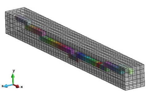
Figure 28: FE mesh and composite material generated

The results of the PLCd analysis are shown in Figures 29 and 30. The first image shows the beam displacements generated by the prestressing force in the vertical direction ${\textstyle y}$. It can be observed that the symmetry of the problem is preserved and that the maximum displacement takes place at the mid-span area, with a value of ${\textstyle 4.41\times 10^{-3}m}$. The second image shows the horizontal shortening that the prestressing steel generates in the beam. The maximum displacement is located at the end where the longitudinal movement is allowed and its value is ${\textstyle -2.34\times 10^{-3}m}$.

Figure 29: Displacement in $y$ direction [m] due to the prestressing effect

Figure 30: Displacement in $x$ direction [m] due to the prestressing effect

For the analytical approach, the prestressing steel effect has been introduced as a set of forces. Figure 31 shows the problem to be solved.

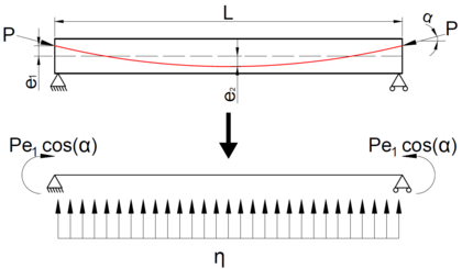
Figure 31: Scheme of the problem to be solved analytically

In this scenario, the vertical displacement is generated by the vertical uniform distributed load (${\textstyle \eta }$) and the bending moments at the edges (${\textstyle M=Pe_{1}\cos(\alpha )}$), i.e. ${\textstyle \delta (x)=f(\eta )+f(M)}$. The maximum deflection will be located at the beam mid span due to the symmetry conditions and can be calculated as [46]:

$\delta _{max}=\delta (x=L/2)={\dfrac {5\eta L^{4}}{384EI}}-{\dfrac {Pe_{1}\cos(\alpha )L^{2}}{8EI}}$

(5.3)

Where ${\textstyle P}$ is the prestressing force of ${\textstyle 5000}$kN, ${\textstyle e_{1}}$ is the tendon eccentricity at the supports (${\textstyle e_{1}=0.3m}$), ${\textstyle L}$ is the beam span (${\textstyle L=10m}$), ${\textstyle \alpha }$ is the tendon angle at the supports sections, which can be computed through the derivative at the support section of the parabolic function that describes the tendon path (${\textstyle y(x)}$):

$y(x)={\dfrac {8e_{1}}{L^{2}}}\left(x^{2}-Lx\right)+e_{1}\Rightarrow y'(0)=\tan(\alpha )=-{\dfrac {8e_{1}}{L}}\Rightarrow \alpha =13.50^{\circ }$

(5.4)

${\textstyle \eta }$ is the vertical distributed load equivalent to the prestressing effect that can be computed as ${\textstyle \eta =Py''(x)={\dfrac {16Pe_{1}}{L^{2}}}=240}$kN/m [10]. Finally, ${\textstyle I}$ is the section inertia in ${\textstyle z}$ direction according to the model reference system, that can be computed as ${\textstyle I={\dfrac {1}{12}}bh^{3}=8.33\cdot 10^{-2}m^{4}}$ and ${\textstyle E}$ is the Young Modulus of the composite section, which can be computed following the procedure used in Equation 5.2, i.e. ${\textstyle E={\dfrac {A_{c}}{A}}E_{c}+{\dfrac {A_{p}}{A}}E_{p}=35.88}$GPa.

Therefore, the maximum deflection is equal to ${\textstyle \delta _{max}=4.36\times 10^{-3}m}$, which is really close to the one computed through the numerical simulation (${\textstyle e_{r}\simeq 1.2\%}$).

Finally, in addition to the displacement evaluation, it is interesting to compare the maximum tension and compression values derived from these two approaches. These points are located at the beam midspan.

5.4 Mock-up of a reactor containment building

The VeRCoRs Project is an initiative promoted by the company Électricité de France (eDF) in which a mock-up of a reactor containment building at ${\textstyle 1/3}$ scale is built and tested.

The construction finished in 2015 and from then several experiments have been conducted. The main objectives of this project are to study [43]:

-

• The behaviour at early age and the ageing of the structure.
• The evolution of the leak tightness under the effect of aging.
• The behaviour under severe accident conditions for which the thermo-mechanical loading is maintained for several days.

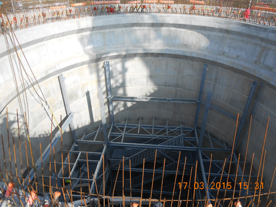
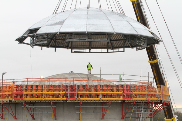
(a) View during construction (March 2015)	(b) External dome lifting (November 2015)
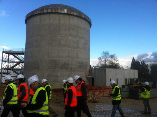
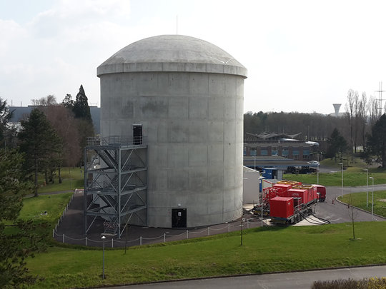
(c) Image taken during the first Benchmark (March 2016)	(d) Image taken before the $5^{th}$ pressure test (March 2018)
Figure 32: Reactor containment building during and after its construction [43]

The project is divided in three phases that have the format of a benchmark. The first one took place in 2015 and it was dedicated to early age, mechanical and leaktightness behaviours. In 2017 the second benchmark started and it has finished in April of 2018. The results presented in this monograph have been obtained from the analysis performed by CIMNE team (A. Barbat, S. Oller, L. Barbu, A. Cornejo and S. Jiménez) at this benchmark, which was oriented towards the study of the mechanical behaviour of the containment during pressurization tests. The last benchmark is planned to take place in 2021 and it will be focused on the behaviour prediction under severe accident conditions.

Problem statement

The mock-up of the reactor containment was built between 2014 and 2015. After finishing the construction and after the prestressing stage, the containment has been subjected to several pressure tests. Table 4 summarizes all the operations done from its construction.

Table. 4 Operation sequence at the mock-up reactor containment building

Operation Sequence
Raft concreting	24 July, 2014
End of construction	06 May, 2015
End of prestressing	17 August, 2015
1st Pressure test ('Pre-op')	04 November, 2015
2nd Pressure test ('VC1')	25 January, 2016
3rd Pressure test ('VD1')	14 March, 2017
4th Pressure test ('VD1 bis')	21 March, 2017
5th Pressure test ('VD2')	02 April, 2018

All the pressure tests follow a similar pattern (Figure 33). First the pressure is increased inside the containment up to ${\textstyle 4.2\,bar}$, it remains constant for a few hours and then it is reduced again to ${\textstyle 0\,bar}$.

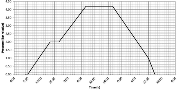
Figure 33: General description of a pressure test

The goal of this benchmark is to predict stresses and strains distribution during the pressure tests.

For the purpose of this monograph, the benchmark format has not been followed exactly. Therefore, not all the results shown here have been included on the benchmark final template and not all the results presented for the benchmark have been included here. Despite this, the main objective is still the same: reproduce the whole procedure and analyse what happens during this time.

Geometry and GiD model

The real structure is composed of two containments, one internal and the other one external (Figure 34). The external one does not have any structural purpose, it is used to provide thermal and humidity protection, and to recreate an annular space for leakage rates measurements (Figure 35). Therefore, for the purpose of this monograph, only the internal structure has been modelled.

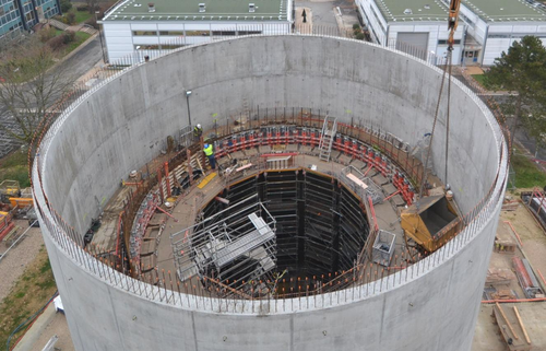
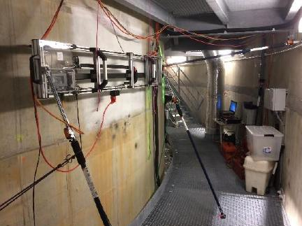
(a) The two containments during construction	(b) Internal corridor with the view of the internal and external walls
Figure 34: Reactor containment building during and after its construction [43]

	]
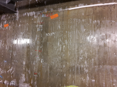Figure 35: Images taken during the leakage tests [43]

The internal structure has the shape of a typical reactor containment but scaled ${\textstyle 1/3}$ (Figure 36). The main dimensions of this structure are summarized in Table 5 and can be compared with the dimensions of a regular containment structure.

Table. 5 Geometric characteristics of the inner containment model

	VeRCoRs model	Regular containment
2-3 Height from gusset to the top [m]	20.79	62.38
Internal radius of cylinder [m]	7.30	21.90
Thickness of cylinder [m]	0.40	1.20
Internal radius of the dome (tore) [m]	2.67	8.00
Internal radius of the dome (centre) [m]	10.67	32.00
Thickness of the dome [m]	0.30	0.90
Free volume inside containment [m3]	3160.00	85350.00

]

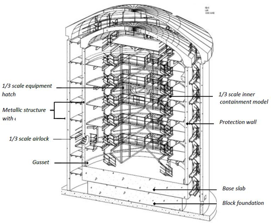Figure 36: General view of the VeRCoRs mock-up [47]

In addition to this, the containment is placed on a two meters thick foundation and it has two vertical prestressing buttresses that are also scaled. There are only two significant openings: one equipment hatch (${\textstyle \Phi =2.71m}$) and one personal airlock (${\textstyle \Phi =1.21m}$)

The prestressing steel system is organised in four families.

• Horizontal tendons (spacing ${\textstyle 133mm}$ in typical area). These tendons go from one buttress to the other one, overcoming the equipment and personal hatches. There are ${\textstyle 122}$ tendons in total and both ends are active.
• Vertical tendons (spacing ${\textstyle 290mm}$ in typical area). These tendons go from the top (ring beam) to the mock-up foundation. There are ${\textstyle 57}$ tendons in total and only one end is active, the lower extreme.
• Dome tendons (spacing ${\textstyle 205mm}$ in the dome). These tendons cross the dome from one side to the other creating a sort of grid. There are ${\textstyle 18}$ tendons in total and both ends are active.
• Gamma tendons (spacing ${\textstyle 205mm}$ in the dome). These tendons are the result of the combination of vertical and dome tendons. Thus, the path that these tendons follow is similar to a ${\textstyle \Gamma }$. There are ${\textstyle 98}$ tendons in total and both ends are active.

The layout is exactly scaled, including any deviations around penetrations and all of them have been cement grouted as in regular structures in France.

Finally, the reinforcing steel is distributed in the whole structure. Rebars spacing and diameters are scaled to keep the same ratios ${\textstyle \rho \,(\%)}$ as in full-size structures. In typical areas of the cylinder, reinforcement principles are alternatively HB 6/8 at 6.7cm in horizontal direction at both inner and outer face, and HB 8/10 at ${\textstyle 0.7^{o}}$ in vertical direction. In the dome, reinforcement principles are also alternatively HB 8/10 at 9.8cm at both faces. The stirrups in the whole containment are made with HB 5.

Using this information and the mock-up plans provided by the company in charge, the GiD model has been built. Figures 37 to 40a show the containment model and the tendons layout for each family.

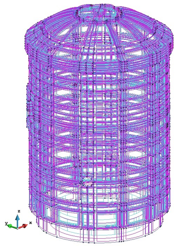
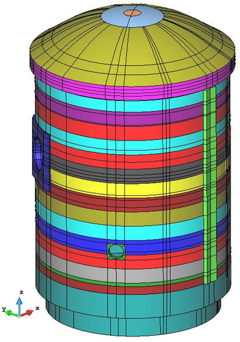
(a) Containment view with normal render from GiD	(b) Containment view with flat render from GiD
Figure 37: GiD geometry of the reactor containment building

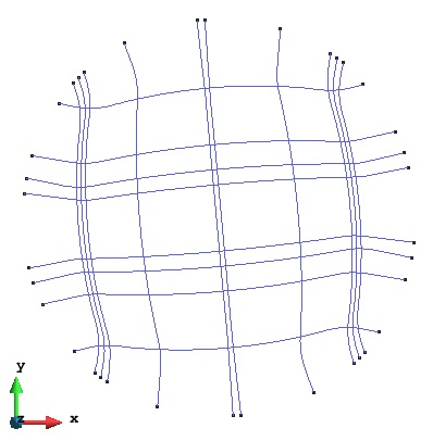
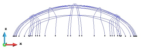
(a) Plan view of the dome tendons	(b) Elevation view of the dome tendons
Figure 38: GiD model with the dome tendons

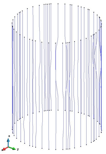
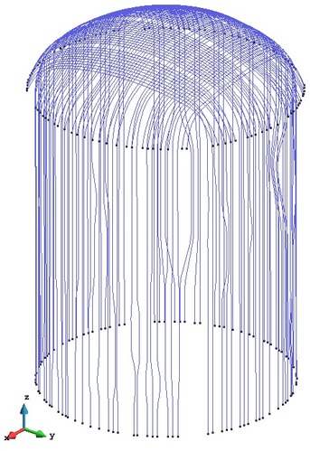
(a) GiD model with the vertical tendons	(b) GiD model with the gamma tendons
Figure 39: GiD model with the vertical tendons and gamma tendons

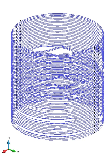
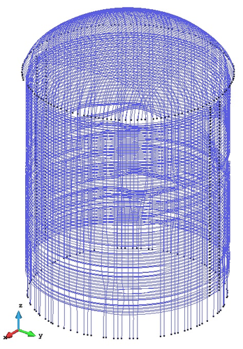
(a) GiD model with the horizontal tendons	(b) GiD model with the prestressing system
Figure 40: GiD model of the horizontal tendons and whole the prestressing system

The reinforcement has not been drawn in the model. The big density of this material within the structure allows including it as an increment in the concrete strength and stiffness.

Material properties, loads and boundary conditions

The company in charge of the mock-up has provided to participants all the material properties referred to concrete, reinforcing steel and prestressing steel. Tables 6, 7 and 8 summarize these values, which have been used in the performed analysis. Figure 41 shows a general view of the containment model and has been selected to facilitate the understanding of Table 6

Table. 6 Concrete properties

CONCRETE
	Young modulus [GPa]	Compressive strength (28 days) [MPa]	Tensile strength (28 days) [MPa]	Density [$kg/m^{3}$]
2-5 Cylinder	34.26	48.68	4.36	2395
Equipment hatch	34.26	48.68	4.36	2395
Personal hatch	34.26	48.68	4.36	2395
Buttresses	39.20	48.68	4.36	2395
Dome	32.51	40.90	4.20	2350
Ring beam	34.26	56.90	4.50	2430
Foundation	33.26	38.50	3.60	2360

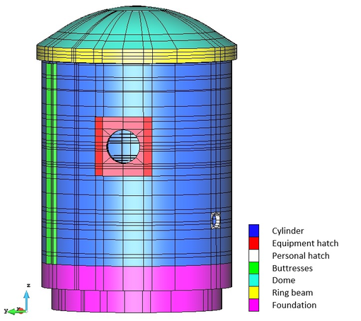
Figure 41: Concrete materials identified at the numerical model

Table. 7 Reinforcing steel properties

REINFORCING STEEL
Yield strength [MPa]	500
Young modulus [MPa]	200000

Table. 8 Prestressing steel properties

PRESTRESSING STEEL
Prestressing system
	System C (4C15) (Fryssinet) ETA-06/0226
	Bonded prestressing
	Pull-in at wedge blocking [mm]		8
Strands
	Strand section (T15) [$mm^{2}$]		139
	Tensile stregth [MPa]		1860
Tendons
	Tendon		4T15
	Tendon maximal prestressing stress (at anchor, before wedge blocking) [MPa]		1488
	Tendon Young modulus [MPa]		190000
Friction
	Vertical tendons	Friction coefficient	0.16
		Wobble coefficient	0.0008
	Horizontal tendons	Friction coefficient	0.17
		Wobble coefficient	0.0015
	Gamma tendons	(Vertical part) Friction coefficient	0.16
		(Vertical part) Wobble coefficient	0.0008
		(Dome part) Friction coefficient	0.16
		(Dome part) Wobble coefficient	0.0015
	Dome tendons	Friction coefficient	0.16
		Wobble coefficient	0.0015

As shown in Table 6, it has been necessary to define seven different concrete materials for the containment. There is no inconvenient in PLCd to define as many materials as the user desires, but the assignation of these properties to the FEs must be done carefully.

Table 7 shows the reinforcing steel properties. As mentioned before, this material has been included in the analysis as indicated in Section 4.3 and thus, its effect is considered as an increment in the concrete strength and stiffness. The magnitude of this effect has been defined per areas depending on the volumetric participation of the reinforcement in each of them. Six regions have been selected: the cylinder, the buttresses, the ring beam, the dome, the hatches and the foundation.

Table 8 contains the information relative to the tensile stress of each tendon and also the parameters required when computing the immediate losses using a standard code (Section 2.1). As mention previously, PLCd cannot compute the immediate loses. In fact it computes the losses due to concrete instantaneous deformation but friction losses and losses due to tendon anchorage are not taken into account.

Therefore, it has been necessary to compute these losses beforehand and use for PLCd the prestressing values after deducting immediate losses. For this uncoupled calculation, a code written in Visual Basic for Applications (VBA) has been developed. It calculates the stress distribution in all the tendons of the mock-up. This is done subtracting the friction losses and the losses due to tendon anchorage from the initial prestressing stress value (${\textstyle 1860}$MPa).

The full code is attached in Appendix 7. It has been created using the formulas proposed at the EHE-08, which have been already presented in Section 2.1. The code main inputs can be obtained from Table 8 and from the model geometry. An example of the final output of this code is displayed at Figures 42 and 43.

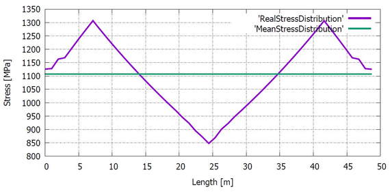
Figure 42: Real and mean stress distribution in a horizontal tendon (H46)

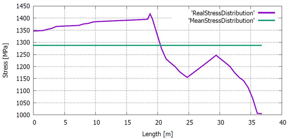
Figure 43: Real and mean stress distribution in a gamma tendon (G155)

It is interesting to see how the RealStressDistribution lines change from one family to the other. Figure 42 has been taken from a horizontal tendon, where the friction losses are significant and the stress distribution is quite symmetric due to the path that these tendons trace. On the other hand, Figure 43 shows the behaviour of a gamma tendon. In this family the stress distribution is asymmetric due to the two different zones that the tendons cross. In fact, the shape of the curve is similar to the addition of the vertical tendons curve (left branch of the graph) and the dome tendons curve (right branch of the graph).

MeanStressDistribution lines are obtained from the RealStressDistribution lines by equalling the areas under the curve. These constant values are the ones that PLCd reads. Although PLCd is prepared to read different prestressing values for each tendon i.e. the MeanStressDistribution values, only one stress value per family has been used for the evaluation of the containment structure. This stress value is obtained as the average of all the MeanStressDistribution values for each family. Table 9 summarizes the result of these operations.

Table. 9 Average stress and strain value per family due to prestressing effect

	Stress [MPa]	Strain
2-3 Horizontal tendons	1087.533	5.72$\times 10^{-3}$
Vertical tendons	1352.632	7.12$\times 10^{-3}$
Dome tendons	1115.099	5.87$\times 10^{-3}$
Gamma tendons	1269.843	6.68$\times 10^{-3}$

In addition to the prestressing effect, the other loads considered for the containment analysis are the self weight and the internal pressure that appears during the five pressure tests. This pressure is applied normal to the model internal surface in GiD considering the containment wall and the hatches (Figure 44a).

Only one boundary condition has been considered for the analysis: the structure is fixed at the base (Figure 44b). This hypothesis is presumably valid as the base slab is anchored in a very thick concrete block that connects the internal and the external structures.

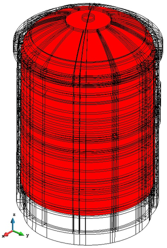
(a) Surface where the pressure is applied	(b) Fixed base of the structure
Figure 44: Loads and boundary conditions at the containment

Finite element mesh

Once the model is complete, the next step is to generate the FE mesh used in the analysis. Figure 45a shows the final layout which consists of ${\textstyle 199600}$ 8-noded hexahedras with linear shape functions. All the FEs have more or less the same dimensions, Figure 45b shows how the elements are distributed in the thickness. This rule is respected everywhere except on the base slab (Figure 45e), where the FEs are bigger. This is because the interest on the slab behaviour during the simulation is reduced and having bigger elements helps to reduce the computational time.

Figures 45c and 45d show a detail of the FE mesh at the dome. It can be seen that there are three volumes there and that the mesh changes from one to another. What is happening is that, while the external ring is meshed following the pattern established in the cylinder, there are two internal crowns that have been meshed using a semi-structured mesh. The use of this strategy allows the generation of an efficient mesh without using too small elements.

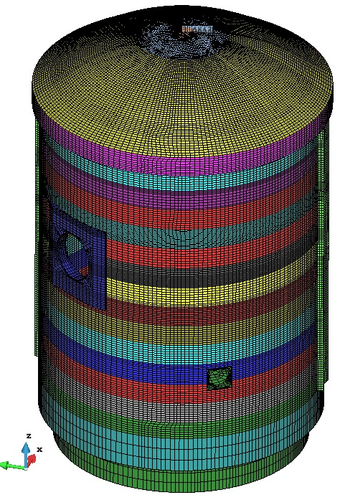
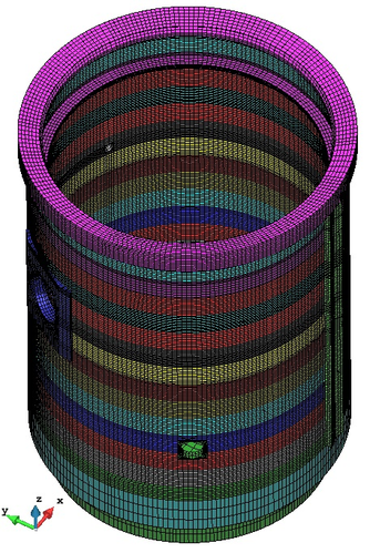
(a) Full structure view	(b) View inside the cylinder and view of the wall thickness
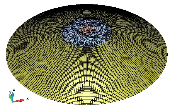
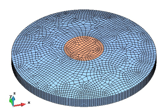
(c) Dome detail	(d) Dome internal region
(e) Foundation detail
Figure 45: FE mesh of the containment model

Results of the analysis

Once the analysis has been performed, there are two kind of results that can be of interest: the global behaviour of the structure and the prestressing steel behaviour. The validation of the results is complex due to the type of structure that is being analysed but there are some aspects that can be predicted:

- The overall behaviour should be:

$\bullet$ Nearly symmetric. The structure is almost symmetrical, therefore, the stress and strain distribution should be also symmetric. The only areas that introduce clear asymmetries to the containment are the hatches in the cylinder wall.

$\bullet$ Invariant in time. The only material with an associated time dependency is the prestressing steel, through the Generalized Maxwell model (see Section 4.3). Therefore, when the global behaviour is analysed, no significant changes will be observed from one pressure test to the next one. Although this is the expected behaviour from the simulation performed, other time dependent effects take place in reality: creep and shrinkage in concrete. The damage model used for concrete modelization does not consider these effects, thus the only way to account for them is using an uncoupled calculation, e.g. using a Generalized Kelvin model [32].

-The prestressing system behaviour is characterized by:

$\bullet$ A progressive decrease in the prestressing tension. The prestressing steel behaviour is reproduced using a Generalised Maxwell model for each tendon family. The company in charge of the benchmark did not give any information that helps to calibrate these models, thus previous experience has been used to build them. CIMNE has analysed the Ascó and Vandellós containments recently¹ and the model parameters used there have been considered here. Table 10 summarizes the Maxwell model parameters for each tendon family and Figure 46 shows the aspect of these curves starting at the anchorage operation moment (${\textstyle t=0}$ years).

Table. 10 Generalized Maxwell model parameters for each tendon family

	Horizontal tendons	Vertical tendons	Dome tendons	Gamma tendons
2-5 Young modulus [MPa]	190000	190000	190000	190000
Initial stress [MPa]	1087.53	1352.63	1115.10	1269.84
$K_{visco}$	0.15	0.15	0.15	0.15

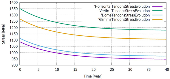
Figure 46: Maxwell model for each family of tendons

$\bullet$ A similar response from one pressure test to another. The prestressing steel has been modelled as a viscoelastic material and therefore, the effect that the pressure will induce in the steel should remain more or less constant in time.

And now, paying attention to this background, results can be explored. Figures 47 to 58 show the stress distribution and the displacement field in the mock-up reactor containment at several points of the analysis: just after introducing the prestressing effect, at the maximum of the first pressure test, at the beginning of the fifth pressure test and at the maximum of the fifth pressure test.

Figure 47: Beginning of the Pre-op test. Displacements [$m$]

Figure 48: Beginning of the Pre-op test. Maximum principal stress - tension stress distribution [$Pa$] at the dome (Cupula) and at the cylinder (Anillo)

Figure 49: Beginning of the Pre-op test. Minimum principal stress - compression stress distribution [$Pa$] at the dome (Cupula) and at the cylinder (Anillo)

Figure 50: Maximum pressure at the Pre-op test. Displacements [$m$]

Figure 51: Maximum pressure at the Pre-op test. Maximum principal stress - tension stress distribution [$Pa$] at the dome (Cupula) and at the cylinder (Anillo)

Figure 52: Maximum pressure at the Pre-op test. Minimum principal stress - compression stress distribution [$Pa$] at the dome (Cupula) and at the cylinder (Anillo)

Figure 53: Beginning of the VD2 test. Displacements [$m$]

Figure 54: Beginning of the VD2 test.Maximum principal stress - tension stress distribution [$Pa$] at the dome (Cupula) and at the cylinder (Anillo)

Figure 55: Beginning of the VD2 test. Minimum principal stress - compression stress distribution [$Pa$] at the dome (Cupula) and at the cylinder (Anillo)

Figure 56: Maximum pressure at the VD2 test. Displacements [$m$]

Figure 57: Maximum pressure at the VD2 test. Maximum principal stress - tension stress distribution [$Pa$] at the dome (Cupula) and at the cylinder (Anillo)

Figure 58: Maximum pressure at the VD2 test. Minimum principal stress - compression stress distribution [$Pa$] at the dome (Cupula) and at the cylinder (Anillo)

It can be observed that the predictions made for the overall structure behaviour are satisfied. The images show a clear symmetric behaviour in both scenarios: with and without internal pressure (Figures 47 and 50).

Furthermore, comparing the images taken from the first pressure test and those from the fifth pressure test, it can be seen that the structure behaves more or less constant in time. Minimum changes can be produced by the damage of the concrete or the prestressing loss, but the overall behaviour remains immutable. The critical areas of the containment are the equipment hatch and the dome where the maximum tensions and compressions are located. The level of stress recorded suggests that damage probably has been activated as will be shown afterwards.

From the previous images it can be conclude that the prestressing system seems to be correctly designed because the overall behaviour remains in compression even when the internal pressure is applied, which is essential in this type of structures.

Finally, Figures 59, 60, 61 and 62 ratify the expected behaviour in the prestressing force evolution. The first chart for all the families shows the progressive decrease of the initial prestressing tension. The other two graphics in each family show a detail of the second, third and fourth pressure tests. Between the second and the third tests there is a time gap of one year in which the Generalized Maxwell model is working, but it can be observed that the effects of each pressure test are nearly the same, only displaced in the Stress-axis.

An interesting effect can be seen that was not considered at the beginning: there are differential behaviours between tendons that belong to the same family. This happens in horizontal tendons (Figure 59) and in dome tendons (Figure 61). Red lines in those graphs are used to point out this phenomena, which can be explained as follows:

• In horizontal tendons, red lines, that are those that show the highest prestressing level, correspond to those tendons located near the containment rigid areas, i.e. the foundation and the ring beam. Therefore, during the pressure tests, these tendons remain more stable.
• In dome tendons, red lines, that are those that show the highest prestressing level, correspond to those tendons that do not go through or near the dome peak. Therefore, during the pressure tests, these tendons remain more stable.

(a) Stress evolution for the whole analysis period

(b) Stress evolution during the second pressurization test

(c) Stress evolution during the third and the fourth pressurization test

Figure 59: Stress evolution at the horizontal tendons

(a) Stress evolution for the whole analysis period

(b) Stress evolution during the second pressurization test

(c) Stress evolution during the third and the fourth pressurization test

Figure 60: Stress evolution at the vertical tendons

(a) Stress evolution for the whole analysis period

(b) Stress evolution during the second pressurization test

(c) Stress evolution during the third and the fourth pressurization test

Figure 61: Stress evolution at the dome tendons

(a) Stress evolution for the whole analysis period

(b) Stress evolution during the second pressurization test

(c) Stress evolution during the third and the fourth pressurization test

Figure 62: Stress evolution at the gamma tendons

In addition to these stress and displacement results of the containment building, PLCd prints the evolution of the damage internal variable ${\textstyle d}$ for each FE. This variable quantifies the damaged volumetric percentage of the finite element but this type of result is not so intuitive.

Therefore, it has been decided to transform this parameter into another one: the crack opening displacement ${\textstyle u_{crack}}$. This new variable is computed inside the FE code at each integration point as:

$u_{crack}=\left(d\cdot \varepsilon _{eq}\right)\cdot l_{f}$

(5.5)

Where ${\textstyle l_{f}}$ is the characteristic length of the element and ${\textstyle \varepsilon _{eq}}$ is the equivalent strain of the integration point, which is computed as:

$\varepsilon _{eq}={\dfrac {{\boldsymbol {\sigma }}:{\boldsymbol {\varepsilon }}}{f\left({\boldsymbol {\sigma }}\right)}}$

(5.6)

Where ${\textstyle f\left({\boldsymbol {\sigma }}\right)}$ is the uniaxial equivalent stress.

This new parameter is an estimation of the maximum crack width that could appear in each FE. Therefore, this is not a function that gives the real crack distribution, but an overview of the problem.

The definition used for this ${\textstyle u_{crack}}$ allows obtaining the crack evolution in the containment building. The presence of cracks depends on the stress state as stated in Equations 5.5 and 5.6 and so it can be observed that ${\textstyle u_{crack}}$ values increase while the pressure tests are being performed but, when there is no internal pressure, these values decrease, i.e. the cracks close. Although this is a realistic behaviour, it is important to keep in mind that the involved materials do not reduce their damage level (${\textstyle d}$ does not decrease) and thus, they do not recover their initial properties.

Figures 63 to 66 show the evolution through the first pressure test of the damage internal variable ${\textstyle d}$ and the crack opening displacement ${\textstyle u_{crack}}$. It is interesting to see that the prestressing operation induces damage to the concrete (Figure 63) and furthermore, it can be seen that the damaged areas match with those with the highest stress state, i.e. the equipment hatch and the dome.

Finally, the evolution in time of these parameters show that the damage effect is accentuated by the rise of the internal pressure, which also leads to an increment in the crack opening displacement.

Figure 63: Beginning of the Pre-op test. Damage internal variable $d\in \left[0,1\right]$ at the dome (Cupula) and at the cylinder (Anillo)

Figure 64: Beginning of the Pre-op test. Crack opening displacement $u_{crack}$ [$m$] at the dome (Cupula) and at the cylinder (Anillo)

Figure 65: Maximum pressure at the Pre-op test. Damage internal variable $d\in \left[0,1\right]$ at the dome (Cupula) and at the cylinder (Anillo)

Figure 66: Maximum pressure at the Pre-op test. Crack opening displacement $u_{crack}$ [$m$] at the dome (Cupula) and at the cylinder (Anillo)

(¹) Cálculo de la vida remanente del sistema de postensado de las centrales nucleares de Ascó y Vandellós y acciones derivadas - CIMNE - Ref.: 16BCX1000154

Conclusions

The analysis of the mock-up reactor containment building helps to visualize the potential of the proposed technique. In this scenario, with a FE mesh of nearly 200000 hexahedras and performing a non-linear analysis with damage in concrete and viscoelasticity in prestressing steel, the computational analysis ran in 10h and 15min, using the CIMNE computational resources (32-threads and 250GB of RAM).

The main advantage of the SP RoM lies in the fact that it works as a manager of constitutive models. Therefore, the user only has to be focused on the accurate definition of the constitutive model of each composite material. The use of the isotropic damage model for the concrete modelization and the viscoelasticity model for prestressing simulation accounts for many of the phenomena that take place in prestressed concrete structures and so are considered appropriate.

The results obtained from the performed analysis match with the ones that were expected. Now its time to see which is the real behaviour of the structure and compare the results obtained through the numerical simulation with those measured in situ during the pressure tests. These results will be provided soon by the company in charge of the benchmark.

It is important to keep in mind the simplifications, the hypothesis considered in this analysis and the possible points to be improved:

• The prestressing sequence has not been considered in the simulation. Thus, all the tendons have been tensioned at the same time. Despite this, the code allows the introduction of the prestressing stage in as many phases as the user desires and take into account this effect in the analysis. Despite this, considering that the simulation lasts for three years while the maximum gap between prestressing operations is of few hours, the inclusion of the prestressing sequence in the analysis has been discarded.

This accuracy level has been used in other cases where the time gaps during the prestressing stage were bigger.

• The FE mesh used in the analysis could be improved. Performing a sensibility analysis changing the model mesh for this structure is quite complex. The algorithm used for the calculation has some restrictions that affect notoriously in the final mesh layout.

The formulation that controls the SP RoM has been written for composite materials with only two component materials: a matrix and a fibre material. The tendon orientation controls the parallel and series behaviour of each element. Therefore, if a FE contains more than one tendon PLCd gives an error message. In general, this can be avoided using a fine FE mesh. Therefore, the maximum FE size is limited.

On the other hand, prestressing steel is included in the model as a truss element with no area information and it is used to compute the intersections needed for the composite elements definition. When the composite generation step (Section 5.2) takes place, the area information is then loaded in order to compute the volumetric participations (${\textstyle {^{f}}k}$ and ${\textstyle {^{m}}k}$). If the FE is smaller than the fibre, then incoherent volumetric participation values are obtained. This happens because the element that is being analysed cannot be simulated as a composite material, it is in fact composed by only prestressing steel. This situation must be avoided and thus, the minimum FE size is controlled by this situation [48].

• Not all the phenomena are predicted. The constitutive models have been chosen in order to reproduce the real behaviour of the structure. Despite this, there are some phenomena that cannot be predicted. This is the case of the time dependent procedures that take place in concrete (creep and shrinkage).

• The prestressing steel effect has been included using a uniform strain value per family. PLCd allows the use of different strain values per tendon but this does not introduce a significant difference in the results that would be obtained because there are no significant differences between the mean stress values of the tendons that belong to the same family.

In addition to this simplification, the numerical simulation cannot compute the instantaneous losses due to friction and wedge blocking. Therefore, this calculation is done uncoupled to the simulation.

• The rheological behaviour of the prestressing steel should be revised. The Maxwell models used for the prediction of the prestressing tension evolution have been defined without any possible calibration. These are based on previous experience in this type of structures, but should be calibrated with the real response of the structure.

Despite this, these drawbacks can be solved and thus, the SP RoM is an interesting technique for the analysis of prestressed concrete structures.

6 Conclusions and future research lines

At this stage, once the bases that support the SP RoM are clear and the applicability of this technique in the analysis of prestressed concrete elements has been shown, some conclusions can be drawn.

The use of this methodology applied to the assessment of this type of structure is quite new. This means that there are still many things that can be improved in order to finally obtain an approach that fully predicts the real behaviour of the prestressed concrete structures. Despite this, the application examples give an accurate idea of the current potential of the methodology and show that it is already a competitive tool.

In fact, compared with the existing alternatives reviewed in Section 2, the SP RoM approach introduces several improvements. The main one is that this technique takes into account the fact that prestressed concrete is a composite material. Therefore, the methodology allows considering concrete and prestressing steel properly in the simulation, i.e. the SP RoM includes physically the tendons into the analysis as the fibre of a LFC. In addition, different constitutive models can be used to predict the behaviour of each component material, which not only allows obtaining the global response, but also the results at each component material. This is really interesting compared to the alternative of using homogenized material properties and interpolation techniques for the analysis of the structure.

On the other hand, in addition to those issues that should be improved in the methodology, there is an important issue related to the accessibility of this FE code that could be considered as a drawback. PLCd is the FE code used for the analysis by means of the SP RoM. It is an extraordinary code which allows performing many type of studies. Despite this, it is not a commercial code and therefore it is difficult to widely distribute the methodology. Thus, the only way to use this approach without using PLCd is by reproducing the code in another FE code.

Some of the issues that should be improved for the proposed methodology are common to other approaches. Therefore, there is a real need to work in those directions and develop feasible solutions. This is the case of the automatic computation of instantaneous prestressing losses or the possibility of considering the prestressing effect with the real stress distribution and not an equivalent constant stress distribution.

Other aspects are specific of the SP RoM. For example, it is convenient to keep working on the correct modelization of the component materials. In this regard, it can be interesting to change from a viscoelsticity model to a viscoplasticity one for the prestressing steel simulation or modify the isotropic damage model to include time-dependent phenomena like creep or shrinkage.

Finally, it would be interesting to improve the methodology and then take part in the last VeRCoRs benchmark. Analysing a structure of this magnitude is an unique opportunity.

References

[1] Oñate, E. (2009) "Structural analysis with the finite element method. Linear statics. Volume 1. Basis and solids"

[2] Cundall, P. and Strack, O. (1979) "A discrete numerical model for granular assemblies", Volume 29. Geotechnique 1 45-65

[3] Oñate, E and Zárate, F. and Miquel, J. and others. (2015) "A local constitutive model for the discrete element method. application to geomaterials and concrete", Volume 2. Computational Particle Mechanics 2 139-160

[4] Franci, A. and Zhang, X. (2018) "3D numerical simulation of free-surface Bingham fluids interacting with structures using the PFEM", Volume 259. Journal of Non-Newtonian Fluid Mechanics 1-15

[5] Otero, F. and Martinez, X. and Oller, S. and Salomon, O. (2015) "An efficient multi-scale method for non-linear analysis of composite structures", Volume 131. Composite Structures

[6] Ministerio de Fomento. (2011) "EHE-08. Instrucción de Hormigón Estructural"

[7] Martínez, X. and Oller, S. and Rastellini, F.G. (2014) "Aplicaciones avanzadas de los materiales compuestos en la obra civil y la edificación". OmniaScience

[8] Rastellini, F. G. (May 2006) "Modelación numérica de la no-linealidad constitutiva de laminados compuestos". UPC-ETSECCPB

[9] Serpieri, R. (November 2005) "A novel constitutive model of composite materials with unidirectional long fibers: theoretical aspects and computational issues". Università degli Studi di Napoli "Federico II"

[10] Murcia, J. and Aguado, A. and others. (1993) "Hormigón armado y pretensado - I"

[11] . (Decembre 2004) "Eurocode 2: design of concrete structures (EN 1992-1-1)"

[12] Ministere de l'Équipment du Logement et des Transports. (September 1992) "Regles techniques de conception et de calculus des ouvrages et constructions en beton precontraint suivant la methode des etats limites - BPEL 91"

[13] Post-Tensioning Institute. (2006) "Post-tensioning manual", $6^{th}$ Edition

[14] Claramunt, D. (2010) "Criterios simplificados para dimensionamiento de elementos pretensados con fisuración controlada". ETSECCPB - UPC

[15] Bairán, J. and Marí, A. and Duarte, N. (2012) "Direct optimal design of partially prestressed concrete for controlled cracking or fatigue". Conference: fib Symposium: Concrete Structures for a Sustainable Community

[16] ACI Committee 318. (2005) "Building code requirements for structural concrete (ACI 318-05) and commentary (ACI 318R-05)"

[17] Marí, A. and Aguado, A. and others. (April 1999) "Hormigón armado y pretensado. Ejercicios"

[18] Aguado, A. and Mirambell, E. and Murcia, E. and Marí, A. (1983) "Problemas de hormigón armado y pretensado". E.T.S. de Ingenieros de Caminos de Barcelona (UPC)

[19] American Association of State Highway and Transportation Officials (AASHTO). (2014) "LRFD bridge design specifications"

[20] Murcia, J. and Aguado, A. and others. (1993) "Hormigón armado y pretensado - II"

[21] Shreedhar, R. and Kharde, R. (February 2013) "Comparative study of Grillage method and Finite Element Method of RCC bridge deck". International Journal of Scientific and Engineering Research

[22] Rodríguez, F.B. (2016) "Comportamiento no lineal de vigas isostáticas de hormigón parcialmente pretensado". ETSECCPB - UPC

[23] Shokoohfar, A. and Rahai, A. (2016) "Nonlinear analysis of pre-stressed concrete containment vessel (PCCV) using the damage plasticity model". Nuclear Engineering and Design

[24] Tavakkoli, I. and Kianoush, M.R. and others. (2017) "Finite element moelling of a nuclear containment structure subjected to high internal pressure". International Journal of Pressure Vessels and Piping

[25] Yapar, O. and Basu, P.K. and Nordendale, N. (2015) "Accurate finite element modeling of pretensioned prestressed concrete beams". Engineering Structures

[26] Briere, V. and Harries, K. A and others. (2013) "Dilation behavior of seven-wire prestressing strand - the Hoyer effect". Construction and Building Materials

[27] "3DS Simulia". https://www.3ds.com/es/productos-y-servicios/simulia/productos/abaqus/

[28] 3DS Simulia. (35.4.1-1 to 35.4.1-6) "ABAQUS 6.14. Analysis user's guide. Volume V: prescribed conditions, constraints and interactions"

[29] Hinton, E. and Owen, D.R.J. (1980) "Introduction to finite element computations"

[30] Cornejo, A. (June 2017) "Numerical simulation of multi-fracture in materials using a coupled FEM-DEM formulation". ETSECCPB-UPC

[31] . (2016) "GID the universal, adaptative and user friendly pre and postprocessing system for computer analysis"

[32] Oller, S. (2014) "Nonlinear dynamics of structures"

[33] Voigt, W. (1889) "Ueber die Beziehung zwischen den beiden Elasticitätsconstanten isotroper Körper". Annalen der Physik

[34] Reuss, A. (1929) "Berechnung der Fliebgrenze von Mischkristallen auf Grund der Plastizitätsbedingung für Einkristalle". ZAMM - Journal of Applied Mathematics and Mechanics

[35] Bishop, J.F.W. and Hill, R. "A theoretical derivation of the plastic properties of a polycrystalline face-centred metal". The London, Edinburgh, and Dublin Philosophical Magazine and Journal of Science

[36] Taylor, G. I. (1938) "Plastic strain in metals". Journal of the Institute of Metals

[37] Oller, Sergio. (April 2003) "Simulación numérica del comportamiento mecánico de los materiales compuestos"

[38] Truesdell, C. and Toupin, R. (1960) "The classical field theories"

[39] Kondo, D. and Welemane, H and Cormery, F. (2007) "Basic concepts and models in continuum damage mechanics". Revue européenne de génie civil

[40] Kachanov, L. (1958) "On the time of fracture under conditions of creep". Izvestia Akademii nauk

[41] Ohno, N. and Wang, J. (1993) "Kinematic hardening rules with critical state of dynamic recovery, Part I: Formulation and basic features for ratcheting behavior". International Journal of Plasticity

[42] Washizu, K. (1974) "Variational methods in elasticity and plasticity". Pergamon Press.

[43] Électricité de France (EDF) "VeRCoRs Project eDF". https://fr.xing-events.com/EDF-vercors-project.html?page=1426249

[44] "GiD the personal pre and post processor". https://www.gidhome.com/

[45] "PLastic Crack dynamic". http://www.cimne.com/PLCd

[46] Canet, J.M. (2012) "Resistencia de materiales y estructuras"

[47] Cobin, M. and Garcia, M. (February 2016) "International Benchmark. VeRCoRs 2015 - Overview, synthesis and lessons learnt". Électricité de France

[48] Cornejo, A and Barbu, L.G. and Escudero, C. and others. (2018) "Methodology for the analysis of post-tensioned structures using a constitutive serial-parallel rule of mixtures", Volume 200. Composite Structures 480-497

Appendix A. Immediate losses