Validation of the particle finite element method (PFEM) for simulation of rock slides in lakes and reservoirs

1. Introduction

The analysis of landslides in reservoirs is particularly interesting because the oscillation of the water surface elevation (especially rapid drawdowns) can foster their occurrence. The existence of the reservoir for a long enough time makes the material of the slopes turn saturated, thus its pore pressure raises and, as a consequence, its effective stress is reduced. This unstabilizing effect is partially compensated by the raise of total stress due to hydrostatic pressure generated by the water in the reservoir. A rapid drawdown eliminates the stabilization in a lapse which is frequently not enough for the pore pressure to be dissipated (this depends on the permeability of the material as well as on the velocity of the water level drop, but is quite frequent). In this situation, the probability of occurrence of a landslide is greater.

Another important feature of this kind of landslides is that they impact against the still water in the reservoir, generating an impulse wave which can cause severe damages in the population and goods placed near the shores. This effect is generated in the same way when the instability happens in lakes or in the sea shore.

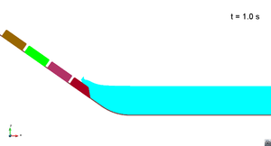
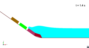
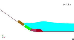
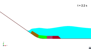
In this report some validation cases are described, where the impact of sliding blocks against a mass of water is simulated, as well as the generation and propagation of the subsequent impulse wave. They are based on the experiments performed by Sælevik et al. [21].

Numerical modeling of this phenomenon is complex because interaction between the sliding mass, the still water in the reservoir and the dam has to be taken into account. It can be considered one of the so-called fluid-structure-interaction (FSI) problems.

Typical difficulties of FSI analysis in free surface flows using the FEM both the Eulerian or Arbitrary Lagrangian Eulerian (ALE) formulation include the treatment of the convective terms and the incompressibility constraint in the fluid equations, the modelling and tracking of the free surface in the fluid, the transfer of information between the fluid and the moving solid domains via the contact interfaces, the modeling of wave splashing, the possibility to deal with large motions of multi-bodies within the fluid domain, the efficient updating of the finite element meshes for both the structure and the fluid, etc. Examples of 3-D analysis of FSI problems using ALE and space-time FEM are reported in [1,2,3,13,3,14,15].

Most of the above problems disappear if a Lagrangian description is used to formulate the governing equations of both the solid and the fluid domains. In the Lagrangian formulation the motion of the individual particles are followed and, consequently, nodes in a finite element mesh can be viewed as moving material points (here forth called “particles”). Hence, the motion of the mesh discretizing the total domain (including both the fluid and solid parts) is followed during the transient solution.

The authors have previously worked in the development of a particular class of Lagrangian formulation for solving problems involving complex interaction between free surface ﬂuids and solids. The method, called the particle finite element method (PFEM, www.cimne.com/pfem), treats the mesh nodes in the ﬂuid and solid domains as particles which can freely move and even separate from the main ﬂuid domain representing, for instance, the effect of water drops. A mesh connects the nodes discretizing the domain where the governing equations are solved using a stabilized FEM.

An advantage of the Lagrangian formulation is that the convective terms disappear from the ﬂuid equations [3,23]. The difficulty is however transferred to the problem of adequately (and efficiently) moving the mesh nodes. We use a mesh regeneration procedure blending elements of different shapes using an extended Delaunay tesselation with special shape functions [5]. The theory and applications of the PFEM are reported in [3,6,10,11,16,17,18,19,20].

2. Overview of the PFEM

Let us consider a domain containing both fluid and solid subdomains (the solid subdomain may include soil/rock materials and/or structural elements). The moving fluid particles interact with the solid boundaries thereby inducing the deformation of the solid which in turn affects the flow motion and, therefore, the problem is fully coupled.

In the PFEM, both the fluid and the solid domains are modelled using an updated Lagrangian formulation [21]. That is, all variables are assumed to be known in the current configuration at time t. The new set of variables in both domains is sought for in the next or updated configuration at time t +Δt. The finite element method (FEM) is used to solve the equations of continuum mechanics for each of the subdomains. Hence a mesh discretizing these domains must be generated in order to solve the governing equations for each subdomain in the standard FEM fashion. The quality of the numerical solution depends on the discretization chosen as in the standard FEM. Adaptive mesh refinement techniques can be used to improve the solution in zones where large motions of the fluid or the structure occur.

2.1 Basic steps of the PFEM

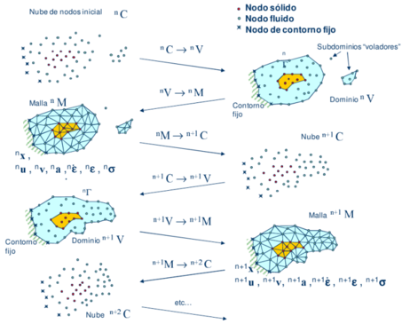
For clarity purposes it will be defined the collection or cloud of nodes (C) belonging to the fluid and solid domains, the volume (V) defining the analysis domain for the fluid and the solid and the mesh (M) discretizing both domains.

A typical solution with the PFEM involves the following steps.

1. The starting point at each time step is the cloud of points in the fluid and solid domains. For instance ⁿC denotes the cloud at time t = t_n (Figure 1).

1. Identify the boundaries for both the fluid and solid domains defining the analysis domain ⁿV in the fluid and the solid. This is an essential step as some boundaries (such as the free surface in fluids) may be severely distorted during the solution, including separation and re-entering of nodes. The Alpha Shape method [6] is used for the boundary definition.

2. Discretize the fluid and solid domains with a finite element mesh ⁿM . PFEM uses an innovative mesh generation scheme based on the extended Delaunay tessellation [7,8,9].

3. Solve the coupled Lagrangian equations of motion for the fluid and the solid domains. Compute the state variables in both domains at the next (updated) configuration for t+ ∆t: velocities, pressure and viscous stresses in the fluid and displacements, stresses and strains in the solid.

4. Move the mesh nodes to a new position ⁿ⁺¹C where n + 1 denotes the time t_n + ∆t, in terms of the time increment size. This step is typically a consequence of the solution process of step 4.

5. Go back to step 1 and repeat the solution process for the next time step to obtain ⁿ⁺²C.

Figure 1. Sequence of steps to update a “cloud” of nodes representing a domain containing a fluid and a solid part from time n(t=t_n) to time n+2 (t=t_n+2∆t). Larese et al. [3].

One of the main tasks in the PFEM is the correct definition of the boundary domain. Boundary nodes are sometimes explicitly identified. In other cases, the total set of nodes is the only information available and the algorithm must recognize the boundary nodes.

3. Experiments

The benchmark experiments carried out by Sælevik et al. [21] were performed in the wave tank at the Hydrodynamics Laboratory at the University of Oslo, in a prismatic channel of 25 m long, 0.51 m wide and 1 m deep.

The sliding masses were simulated with rigid box modules of 0.5 and 0.6 m long, covering slide lengths of 1, 1.6 and 2 m. The boxes were connected, and the gap between them was around 5 cm, that allows the slide to bend. The thickness of the boxes was 0.12 m in one of the tests and 0.16 m in the other two. The width (this parameter is not important as the study carried out was in two dimensions) was the same in all scenarios (0.45 m), as well as the front angle, fixed to 45º.

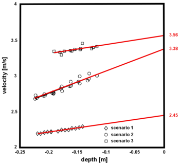
A conveyor belt was used to accelerate the boxes before they entered the slide panel. At the entrance of the slide plane, guiding walls were assuring that the boxes entered the slide plane correctly. In the experiment the velocities of the boxes along the slide plane at impact were estimated by optically tracking the front of the boxes. The trend for all three scenarios was close to linear, thus the impact velocity of the boxes was found by linear extrapolation.

The estimated velocities are presented in Figure 3.

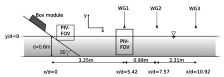
The water depth in the model was 0.6 m, and the slide plane angle is 35º. The transition from the slide plane to the bottom of the tank was rounded (the radius is not specified in [21]). Figure 2 shows schematically the disposal of all the elements in the experiments. In the figure it can be seen the box module, the ramp angle, the water depth and the location of WG1, WG2 and WG3, which are three sensors that measure the evolution of the free surface over time.

Figure 2. Scheme of the experiments conducted by Sælevik et al. [21].

Figure 3. Estimation of the box velocity and linear fit. Adapted from Sælevik et al. [21].

The geometrical parameters and estimated velocities at impact for each scenario are summarized in Table 1.

Table 1. Summary of the parameters with regard to the geometry and kinematics of the blocks in the experiments. Adapted from Sælevik et al. [21].

Scenario	Height [m]	Total length [m]	Impact velocity [m/s]
1	0.16	2	2.45
2	0.16	1	3.38
3	0.12	1.6	3.56

4. Numerical simulation

All three scenarios studied by Sælevik et al. [21] were simulated using the PFEM. The geometry of the blocks and the channel were reproduced according to the published information. However, the kinematics of the sliding blocks is not fully defined in the references. Only the variation of velocity over time before the impact was recorded, thus there is not information about the behavior of the blocks once submerged. The numerical simulations have been set assuming that the blocks impact into the water with the same velocity as in the experiments (velocity at depth=0 in Figure 3). That velocity is assumed to be constant until all the blocks reach the bottom of the tank.

The parameters used in the simulations are shown in Table 2.

Table 2. Summary of the slide parameters in the numerical model.

Scenario	Height [m]	Total length [m]	Impact velocity [m/s]
1	0.16	4 blocks of 0.5*	2.45
2	0.16	2 blocks of 0.5*	3.38
3	0.12	2 blocks of 0.5 and 1 of 0.6*	3.56

(*)The gap between blocks was considered of 0.05 m.

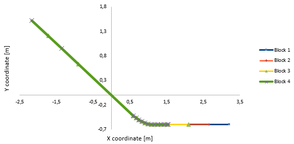
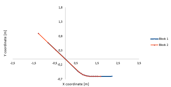
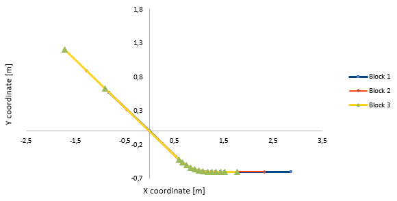
In the numerical model, the abovementioned velocity is imposed by means of appropriate time-series of the position of the front, formed by triplets (coordinates, angle and time). Figures 4, 5 and 6 show the points considered to describe the movement.

The position of the front over time can be easily calculated from the assumption made with regard to the velocity of the blocks. A spreadsheet has been elaborated to generate the values of the triplets for each scenario, which was passed to PFEM (Table 3).

Figure 4 shows the trajectory of the front point of the blocks in scenario 1. The points taken into account to define the movement are sketched in the graph. The difference between the three scenarios (Figures 4, 5 and 6) can be easily appreciated paying attention to the end point.

Figure 4. Position of the frontal point of each block in scenario 1, used to define the movement.

Figure 5. Position of the frontal point of each block in scenario 2, used to define the movement.

Figure 6. Position of the frontal point of each block in scenario 3, used to define the movement.

Table 3. Position of the frontal point for the first block at different instants. Scenario 1.

Time (s)	X coordinate (m)	Y coordinate (m)
0.00	-0.819	0.574
0.82	0.000	0.000
1.11	0.599	-0.419
1.15	0.672	-0.466
1.19	0.750	-0.506
1.22	0.830	-0.540
1.26	0.913	-0.566
1.29	0.999	-0.585
1.33	1.085	-0.596
1.36	1.172	-0.600
1.40	1.260	-0.600
1.44	1.349	-0.600
1.47	1.437	-0.600
1.51	1.525	-0.600
2.19	3.202	-0.600

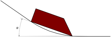
Once the movement is defined it is necessary to describe the evolution of the angle formed by the bottom of each block and the horizontal plane. That parameter was calculated geometrically using GiD. The angle is measured as depicted in Figure 7.

Figure 7. Angle formed by the bottom of the block and the horizontal plane.

Table 4 shows the evolution of the angle of the first block over time in scenario 1. It should be noticed that the blocks start the movement forming a 35º angle with the horizontal plane, so the angle that has to be provide to PFEM is the angle α shown in Figure 7 minus the initial angle (35º).

Table 4. Angle at each moment for the first block. The data provided to PFEM are the first and the third columns. Scenario 1.

Time	Angle α (º)	Angle (α - 35º)
0.00	35.00	0.00
1.11	35.00	0.00
1.15	34.56	-0.44
1.19	33.26	-1.74
1.22	31.10	-3.91
1.26	28.07	-6.93
1.29	24.20	-10.80
1.33	19.48	-15.52
1.36	14.48	-20.52
1.40	9.84	-25.16
1.44	6.06	-28.94
1.47	3.19	-31.81
1.51	1.24	-33.76
1.76	0.00	-35.00

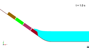
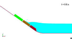
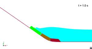
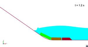
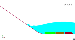
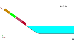
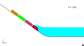
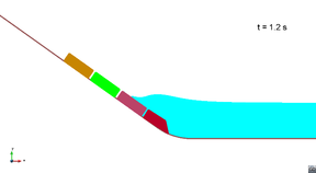
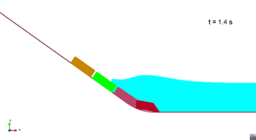
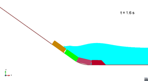
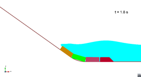
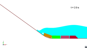
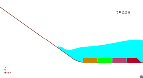
Figure 8 shows the movement of the blocks along the slide ramp in scenario 1. It can be seen that there is a small overlap between the blocks when they are in the rounded part. This is because the gap between the lower part of the blocks was considered constant (5 cm).

Figure 8. Results of the simulation of scenario 1.

5. Results and discussion

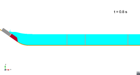
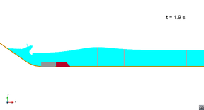
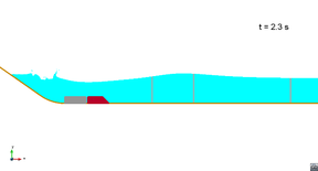
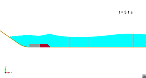
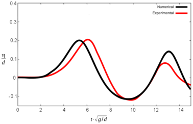
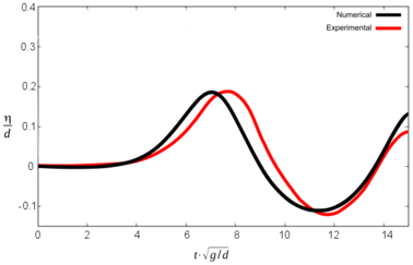
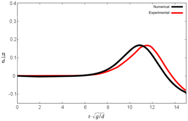
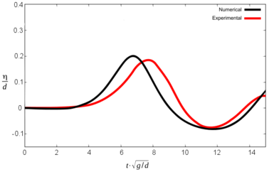
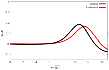
For all scenarios, the features of the leading wave were used to compare the results between experimental and numerical simulation. Sælevik et al. [21] provide data of the evolution of the free surface in the three sensors defined in Figure 2. PFEM allows users to set the position of a number of sensors for storing the free surface elevation in every time step, thus they have been situated coinciding with the gauges in the experiment. Figure 9 shows the evolution of the free surface in the three sensors in different instants during scenario 2.

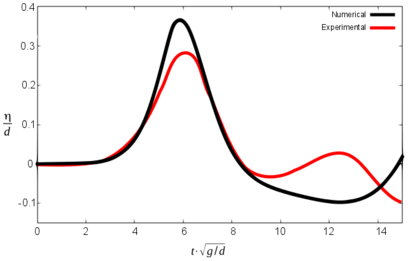
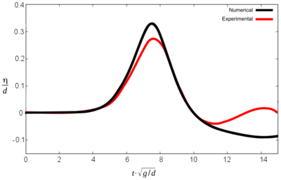
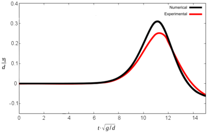
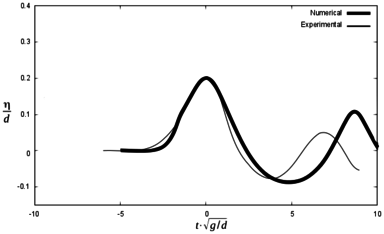
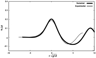
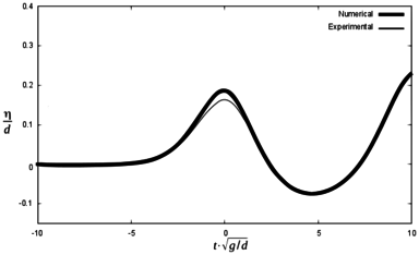
Figure 9. Free surface evolution in scenario 2.

Figures 10, 11 and 12 show the comparative graphs of the experimental results and those obtained with PFEM for scenario 1, 2 and 3 respectively.

It is important to note that in this graphs the origin of time-axis coincides with the instant when the front impacts the water (in opposition to Tables 3 and 4, where t was set to zero at the beginning of the simulation).

Figure 10. Comparison between the results of the physical model (taken from Sælevik et al. [21], red line) and the PFEM calculation (black line) for scenario 1. From top to bottom, sensors WG1, WG2 and WG3 (see location in Figure 2). η = free surface elevation (m), d = initial water depth (0.6 m), t = time (s), g = gravitational acceleration (m/s²).

Figure 11. Comparison between the results of the physical model (taken from Sælevik et al. [21], red line) and the PFEM calculation (black line) in scenario 2. From top to bottom, sensors WG1, WG2 and WG3 (see location in Figure 2). η = free surface elevation (m), d = initial water depth (0.6 m), t = time (s), g = gravitational acceleration (m/s²).

Figure 12. Comparison between the results of the physical model (taken from Sælevik et al. [21], red line) and the PFEM calculation (black line) in scenario 3. From top to bottom, sensors WG1, WG2 and WG3 (see location in Figure 2). η = free surface elevation (m), d = initial water depth (0.6 m), t = time (s), g = gravitational acceleration (m/s²).

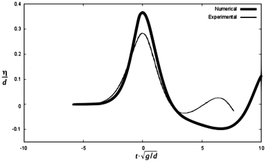
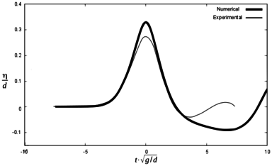
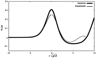
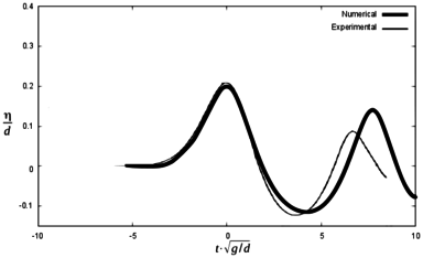
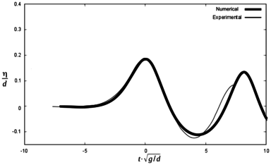
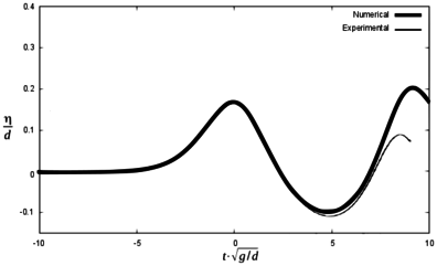
In order to check difference between the maximum height of the first wave in the experiments and in the numerical simulations, Figures 13, 14 and 15 are presented below. They represent the same scenarios 1, 2 and 3, but time axis was shifted so that the maximum wave height coincided between numerical and experimental results. Zero time is considered to be the time for the maximum free surface elevation at each gauge.

Figure 13. Comparison between the first wave elevation of the physical model (taken from Sælevik et al. [21], finer line) and the PFEM calculation (wider line). From top to bottom, sensors WG1, WG2 and WG3 (see location in Figure 2) in scenario 1. η = free surface elevation (m), d = water depth (0.6 m), t = time (s), g = gravitational acceleration (m/s²). Zero time is considered to be the time for the maximum free surface elevation at WG1.

Figure 14. Comparison between the first wave elevation of the physical model (taken from Sælevik et al. [21], finer line) and the PFEM calculation (wider line). From top to bottom, sensors WG1, WG2 and WG3 (see location in Figure 2) in scenario 2. η = free surface elevation (m), d = water depth (0.6 m), t = time (s), g = gravitational acceleration (m/s²). Zero time is considered to be the time for the maximum free surface elevation at WG2.

Figure 15. Comparison between the first wave elevation of the physical model (taken from Sælevik et al. [21], finer line) and the PFEM calculation (wider line). From top to bottom, sensors WG1, WG2 and WG3 (see location in Figure 2) in scenario 3. η = free surface elevation (m), d = water depth (0.6 m), t = time (s), g = gravitational acceleration (m/s²). Zero time is considered to be the time for the maximum free surface elevation at WG3.

It can be seen that the numerical model reproduces the results of the experiment with certain discrepancies both in terms of wave height and the time for maximum free surface elevation. Table 5 summarizes the results.

Table 5. Summary of results. Zero time is considered to be the time for the first block to reach the water.

Sc 1	Max. wave height (m)
	G1 ex	G1 num	Dif (%)	G2 ex	G2 num	Dif (%)	G3 ex	G3 num	Dif (%)
	0.168	0.216	28.6	0.165	0.198	20	0.156	0.186	19.2
	Time for maximum wave (s)
	G1 ex	G1 num	Dif (s)	G2 ex	G2 num	Dif (s)	G3 ex	G3 num	Dif (s)
	1.51	1.43	0.08	1.90	1.83	0.07	2.77	2.72	0.05
Sc 2	Max. wave height (m)
	G1 ex	G1 num	Dif (%)	G2 ex	G2 num	Dif (%)	G3 ex	G3 num	Dif (%)
	0.126	0.120	4.8	0.114	0.114	0	0.102	0.102	0
	Time for maximum wave (s)
	G1 ex	G1 num	Dif (s)	G2 ex	G2 num	Dif (s)	G3 ex	G3 num	Dif (s)
	1.48	1.29	0.19	1.90	1.73	0.17	2.87	2.70	0.17
Sc 3	Max. wave height (m)
	G1 ex	G1 num	Dif (%)	G2 ex	G2 num	Dif (%)	G3 ex	G3 num	Dif (%)
	0.120	0.120	0	0.111	0.120	8.1	0.102	0.111	8.8
	Time for maximum wave (s)
	G1 ex	G1 num	Dif (s)	G2 ex	G2 num	Dif (s)	G3 ex	G3 num	Dif (s)
	1.48	1.24	0.24	1.90	1.66	0.24	2.84	2.62	0.22

In previous sections, special attention has been paid to the kinematics of the blocks, given that there is not enough information in the references to characterize it completely. It has been set taking some assumptions, what leads to differences between the numerical and the experimental models. This discrepancy can be the cause of the mismatch between the results in terms of both the maximum wave height and the arrival time.

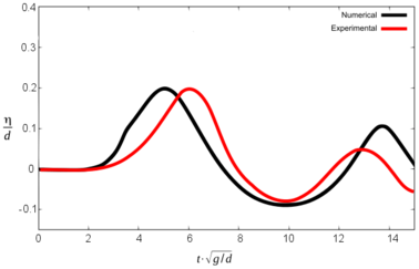
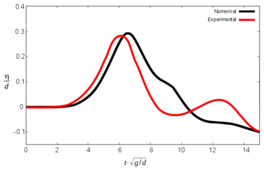
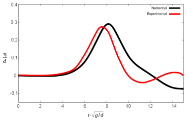
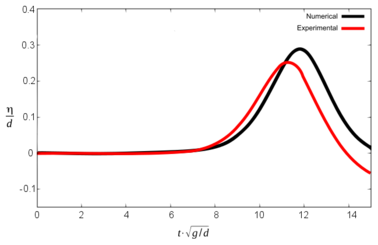
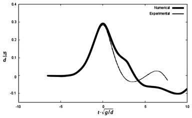
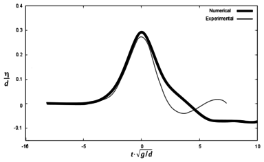
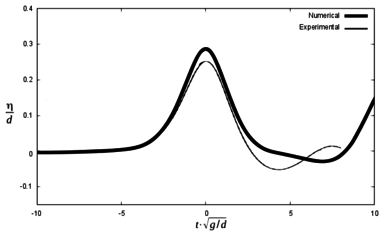
A further numerical simulation (run 2) has been performed in order to check the influence of the kinematics of the blocks in the results. It reproduces scenario 1, but the velocity of the blocks is set to decrease linearly once they enter into the water (instead of being constant until they stop, as before). Figures 16 and 17 show the results.

Figure 16. Comparison between the results of the physical model (taken from Sælevik et al.[21], red line) and the PFEM (black line). From top to bottom, sensors WG1, WG2 and WG3 in scenario 1, run 2 (see location in Figure 2). η = free surface elevation (m), d = water depth (0.6 m), t = time (s), g = gravitational acceleration (m/s²).

Figure 17. Comparison between the first wave elevation of the physical model (taken from Sælevik et al. [21], finer line) and the PFEM (wider line). From top to bottom, sensors WG1, WG2 and WG3 in scenario 1, run 2 (see location in Figure 2). η = free surface elevation (m), d = water depth (0.6 m), t = time (s), g = gravitational acceleration (m/s²). Zero time is considered to be the time for the maximum wave height at each gauge.

As expected, the results are much closer to the experiments, both for the maximum wave height and for the arrival time. Table 6 shows the results, in comparison with previous ones.

Table 6. Comparison of results between both runs of scenario 1.

Sc 1. Run 1	Max. wave height (m)
	G1 ex	G1 num	Dif (%)	G2 ex	G2 num	Dif (%)	G3 ex	G3 num	Dif (%)
	0.168	0.216	28.6	0.165	0.198	20	0.156	0.186	19.2
	Time for maximum wave (s)
	G1 ex	G1 num	Dif (s)	G2 ex	G2 num	Dif (s)	G3 ex	G3 num	Dif (s)
	1.51	1.43	0.08	1.90	1.83	0.07	2.77	2.72	0.05
Sc 1. Run 2	Max. wave height (m)
	G1 ex	G1 num	Dif (%)	G2 ex	G2 num	Dif (%)	G3 ex	G3 num	Dif (%)
	0.168	0.174	3.6	0.165	0.174	5.5	0.156	0.171	9.6
	Time for maximum wave (s)
	G1 ex	G1 num	Dif (s)	G2 ex	G2 num	Dif (s)	G3 ex	G3 num	Dif (s)
	1.51	1.61	0.10	1.90	2.05	0.15	2.77	2.89	0.12

7. Summary and Conclusions

The physical experiments carried out by Sælevik et al [21], representing a falling mass impacting against a mass of water, have been reproduced with the PFEM. The sliding mass is considered as a set of rigid solids in all the simulations, in accordance with the experiments (PFEM can also consider landslides moving as a fluid with given density, as described in [20]).

The three different scenarios run by Sælevik where reproduced numerically. Both the geometry and the physics of the experiments were considered in the numerical model, except the kinematics of the sliding blocks, which had to be estimated. The maximum wave height recorded in the numerical simulation matches the experimental results within 0.0 to 8.8% for scenarios 2 and 3. Discrepancies in scenario 1 are larger (up to 28.6%).

The influence of the kinematics of the blocks was assessed by repeating the simulation of scenario 1 with a different estimation of the velocity: it was set so that it decreases linearly once the last block reaches the bottom of the channel. Table 7 summarizes the results.

Table 7. Summary of the results. Difference in the maximum wave height between the physical experiments and the numerical simulations.

Scenario	Run	Difference in maximum wave height (%)
Scenario	Run	WG1	WG2	WG3
1	1	28.6	20.0	19.2
2	1	4.8	0.0	0.0
3	1	0.0	8.1	8.8
1	2	3.6	5.5	9.6

It can be seen that the discrepancies between the experimental and the numerical results are reduced in the second run for scenario 1, what suggest that the inexact definition of the velocity of the blocks can be the cause of the mismatch in the results.

In spite of that, results show that PFEM can be used for the numerical simulation of sliding blocks impacting against a mass of still water, providing useful results in terms of the maximum wave height and the arrival time. The inaccuracy in the results is neatly lower than the uncertainty associated with the analysis of the phenomenon (due to the lack of precise information about the geometry and geotechnical features of the potentially unstable mass).

Although the cases presented were run in 2D, the same numerical scheme can be directly applied to 3D cases, with no extra complexity in the model.

References

[1] Baiges J., Codina R. (2010). The fixed-mesh ALE approach applied to solid mechanics and fluid-structure interaction problems. Int. J. Num. Methods Eng. 81:1529–1557

[2] Bazilevs Y., Hsu M-C., Zhang Y., Wang W., Liang X., Kvamsdal T., Brekken R., Isaksen, J. (2010). A fully coupled fluid–structure interaction simulation of cerebral aneurysms. Comput Mechan 46: 3–16

[3] Carbonell, J. M., Oñate, E. & Suárez, B. (2010). Modeling of ground excavation with the Particle Finite Element Method. Journal of Engineering Mechanics (ASCE) 136(4):455–463

[4] Donea J., Huerta A. (2003). Finite element method for flow problems. Wiley, Chichester.

[5] Idelsohn, S.R., Oñate, E., Calvo, E.N. & Del Pin, F. (2003a). The meshless finite element method. Int. J. Num. Meth. Eng. 58(6) 893-912

[6] Edelsbrunner H., Mucke E.P. (1999). Three dimensional alpha shapes. ACM Trans Graphics 13:43–72

[7] Idelsohn S.R., Oñate E., Calvo N., Del Pin F. (2003). The meshless finite element method. Int J Numer Methods Eng 58(6):893–912

[8] Idelsohn S.R., Calvo N., Oñate E. (2003). Polyhedrization of an arbitrary point set. Comput Methods Appl Mech Eng 192(22– 24):2649–2668

[9] Idelsohn S.R., Oñate E., Del Pin F. (2004). The particle finite element method: a powerful tool to solve incompressible flows with free-surfaces and breaking waves. Int J Numer Methods Eng 61: 964–989 21

[10] Idelsohn, S. R., Oñate, E. y Del Pin, F. (2003b). A lagrangian meshless finite element method applied to fluid-structure interaction problems. Comput. Struct. 81 (2003) 655-671

[11] Idelsohn, S.R., Oñate, E., Del Pin, F. y Calvo, N. (2006). Fluid-structure interaction using the particle finite element method. Computer Methods in Applied Mechanics and Engineering, 195, pp. 2100-2123

[12] Larese A., Rossi R., Oñate E., Idelsohn S.R. (2008). Validation of the particle finite element method (PFEM) for simulation of free surface flows. Eng Comput 25(4):385–425

[13] Löhner R. (2008) Applied CFD techniques. Wiley, Chichester

[14] Oñate E., García J. (2001) .A finite element method for fluid– structure interaction with surface waves using a finite calculus formulation. Comp. Methods Appl. Mech. Eng. 191:635–660

[15] Oñate E., García J., Idelsohn S.R., Del Pin F. (2006). FIC formulations for finite element analysis of incompressible flows Eulerian, ALE and Lagrangian approaches. Comput. Methods Appl. Mech. Eng. 195(23–24):3001–3037

[16] Oñate E., García, J. (2001). A ﬁnite element method for ﬂuid-structure interaction with surface waves using a ﬁnite calculus formulation. Comput. Meth. Appl. Mech.Engrg. 191:635–660

[17] Oñate, E., Idelsohn, S. R., Del Pin, F. & Aubry, R. (2004). The particle ﬁnite element method. An overview. Int. J. Comput. Methods 1(2):267–307

[18] Oñate E., Celigueta, M. A. & Idelsohn, S. R. (2006). Modeling bed erosion in free surface ﬂows by the Particle Finite Element Method, Acta Geotechnia 1(4):237–252

[19] Oñate, E., Idelsohn, S.R, Celigueta, M.A., & Rossi, R. (2008). Advances in the particle finite element method for the analysis of fluid-multibody interaction and bed erosion in free surface flows. Comp. Methods in Apll. Mech. And Eng., Vol. 197, 1777-1800

[20] Salazar, F., Oñate, E. & Morán, R. (2011). Modelación numérica de deslizamientos de ladera en embalses mediante el método de partículas y elementos finitos (PFEM). Rev. Int. Mét. Num. Cálc. Dis. Ing. 2012; 28(2):112-123

[21] Sælevik, G., Jensen, A. Pedersen, G. (2009). Experimental investigation of impact generated tsunami; related to a potential rock slide, Western Norway. Coastal Engineering. 56 (2009) pp: 897-906

[22] Zienkiewicz O.C., Taylor R.L. (2005). The finite element method for solid and structural mechanics. Elsevier, Oxford

[23] Zienkiewicz, O., Taylor, R. L. & Nithiarasu, P. (2006). The finite element method for fluid dynamics. Elsevier

Appendix. Results of the numerical simulations

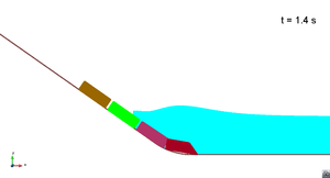
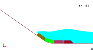
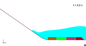
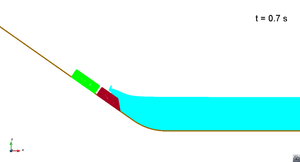
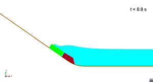
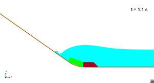
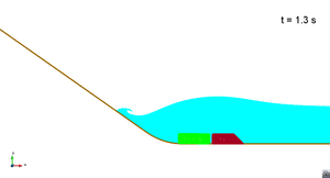
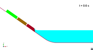
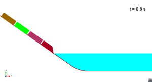
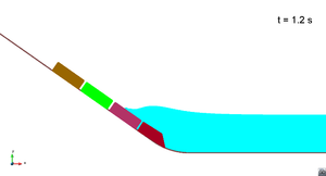
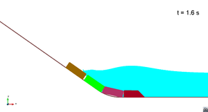
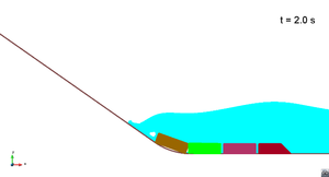
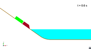
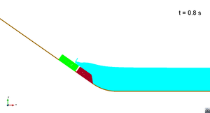
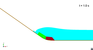
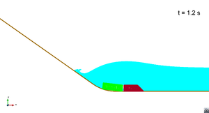
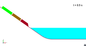
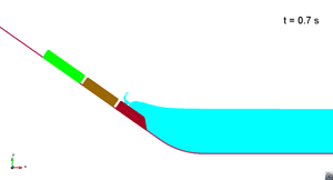
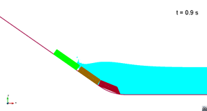
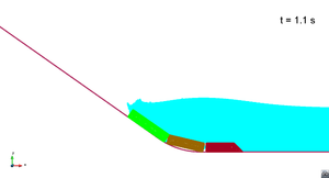
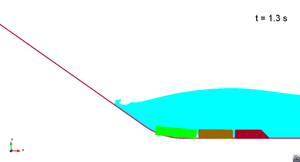
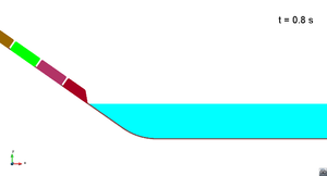
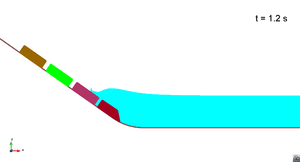
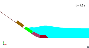
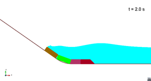
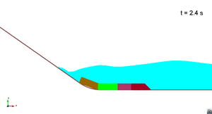
In this appendix some images from the numerical simulations are presented. For each scenario and run, two set of images are included; first, a detailed view of the impact of the blocks against the water and the wave generation; then, an overall view of the wave propagation.