Climatology and interannual variability of the annual mean Hadley circulation in CMIP5 models

Abstract

Using 26 climate models from the Coupled Model Intercomparison Project Phase 5 (CMIP5), climatology and the interannual variability of the annual mean Hadley circulation are evaluated. The results show that most of 26 models perform well in simulating the spatial structure of the climatology of the annual mean Hadley circulation, but the results derived from these models are generally weaker than that derived from the reanalysis dataset. Eighteen models can properly simulate well the asymmetric mode and symmetric mode of the annual mean Hadley circulation variability. Two models can only simulate asymmetric mode or symmetric mode and the other two models simulate reversed sequences of asymmetric mode and symmetric mode.

The possible reason why some models cannot properly simulate the asymmetric mode and symmetric mode is that these models do not properly simulate the structure of zonal mean sea surface temperature (SST). Especially, not properly simulating variances of symmetric and asymmetric components of the SSTA will lead to reversed sequence of symmetric mode and asymmetric mode. And not properly simulated either symmetric or asymmetric component of the SSTA will lead to inability in simulating symmetric mode or asymmetric mode. On the other hand, some models properly simulate the asymmetric mode and symmetric mode, but do not properly simulate the responses to SST change. These models can not reflect the air sea coupling processes in associated with the Hadley circulation, therefore they should be taken more care when classify the models into groups.

Keywords

Hadley circulation ; CMIP5 models ; Symmetry ; Meridional SST gradient

1. Introduction

As one of the most important large-scale circulations in the tropics, Hadley circulation (HC) plays an important role in modulating the climate system, such as the hydrological process (Schneider et al., 2010 ), the subtropical droughts (Fu et al., 2006 ), the tropical cyclone (Zhang and Wang, 2013  and Zhang and Wang, 2015 ) and the extratropical climate (Hou, 1998 ). Due to the importance of HC research, more and more attentions have been paid to the changes of HC in recent years.

Although there are many studies discussing the changes of HC, no consensus has been reached about the changes of HC intensity. Using the observational datasets, some studies showed that the intensity of the annual mean HC increased in the 1990s (Chen et al., 2002  and Wielicki et al., 2002 ). However, some subsequent studies reported that the intensity of HC is seasonally dependent. In the boreal winter (December, January and February, DJF), HC has strengthened since the 1950s (Quan et al., 2004 , Ma and Li, 2007 , Ma and Li, 2008 , Feng et al., 2013  and Mitas and Clement, 2005 ); Feng et al. (2013) further pointed out that in boreal spring, the HC also intensified; but some other studies revealed that the strength of the HC in boreal summer shows no significant increasing trend (Tanaka et al., 2004  and Feng et al., 2011 ).

In addition to the intensity, the HC width also attracts lots of attentions. It is reported that the HC has a poleward expansion trend since 1979 (Fu et al., 2006 , Frierson et al., 2007 , Lu et al., 2007 , Seidel et al., 2008  and Hu and Fu, 2007 ; Hu et al., 2011  and Johanson and Fu, 2009 ). The widening of the HC results in a poleward extension of the subtropical dry zones (Polvani et al., 2011 ).

Given the fact that HC has important climate impacts, its spatial structure is also worth investigating. Dima and Wallace (2003) found that the annual march of HC is consisted of two components: the asymmetric and symmetric parts. Subsequently, Ma and Li (2008) found that the principal modes of the year-to-year variability of DJF HC show asymmetric mode (AM) for EOF1 and symmetric mode (SM) for EOF2. Similar results were also obtained in boreal summer and spring (Feng et al., 2011 , Feng et al., 2013  and Li et al., 2013 ). Feng and Li (2013) pointed out that the classical El Niño events have different impact on HC structure from that of the El Niño Modoki events. The former can lead to symmetric HC anomaly, while the latter will lead to asymmetric HC anomaly. The asymmetric HC anomaly is documented to have impacts on subtropical precipitation (Feng et al., 2013  and Li et al., 2015 ) and tropical cyclone (Zhang and Wang, 2013 ).

The above mentioned studies indicate that the HC variability is complex and has important climate impacts. Understanding the HC variability and its future change are quite necessary. However, the trends of the HC are inconsistent among different datasets because of the atmospheric thermal structure bias (Stachnik and Schumacher, 2011 , Nguyen et al., 2013  and Mitas and Clement, 2006 ). To better understand how HC changes, the high-performance numerical models are needed. The Coupled Model Intercomparison Project Phase 5 (CMIP5) provides useful benchmark for evaluating the state-of-art coupled models' performance in simulating the climate system. Previous studies demonstrated that the current climate models underestimated the poleward expansion of the HC (Hu et al., 2013  and Quan et al., 2014 ). Feng et al. (2015) even pointed out that no models can capture the long-term trend in the AM of annual mean HC due to the failure in simulating the interhemispheric sea surface temperature (SST) difference among the 10 CMIP5 models they selected. Hence, it is important to analyze the climatology and interannual variability of the annual mean HC simulation by using more CMIP5 models.

In this paper, 26 CMIP5 models were employed to evaluate their ability in reproducing the observed climatology and interannual variability of the annual mean HC. In addition, the SST anomaly (SSTA) patterns corresponding to the HC principal modes were also analyzed. The remainder of the manuscript is arranged as follows: Section 2 described the reanalysis data, the CMIP5 models and the methods; Section 3 presented the results. Discussion and conclusions were given in Section 4 .

2. Data, model description and methods

2.1. Data and methods

The atmospheric variables were employed from the Interim European Centre for Medium-Range Weather Forecasts (ECMWF) Re-Analysis (ERAI), which has time coverage from 1979 to present, with a 2.5° × 2.5° horizontal resolution and 37 vertical levels (Dee et al., 2011 ). The SST data used in this study is from the monthly mean Extended Reconstruction of Historical Sea Surface Temperature version 3b (ERSST v3b) dataset, which has a 2.0° × 2.0° horizontal resolution and covers the period from 1854 to present (Smith et al., 2008 ).

We use mass stream function (MSF) to represent the HC, which is calculated by integrating the zonal mean meridional wind (Holton, 1992  and Li, 2001 ). The empirical orthogonal function (EOF) analysis is used to extract the principal modes HC.

2.2. Model description

We employed 26 CMIP5 models (https://pcmdi9.llnl.gov , Taylor et al., 2012 ) in this study, and the further details are listed in Table 1 . The first realizations of the historical experiments were used to make each model have equal weight in the multi-model ensemble (MME) mean. All the outputs from the atmospheric components were interpolated to a 2.5° × 2.5° common grid and the outputs from the ocean components were interpolated on to a 2.0° × 2.0° common grid for the convenience to compare with the observations. The study period is 1979–2005, which is the overlapped period of all datasets.

Table 1. A brief introduction of the CMIP5 models used in this study.

Model	Institution and country	Layers	Atmospheric resolution
bcc-csm1-1	Beijing Climate Center, China Meteorological Administration	26	128 × 64
CESM1-CAM5	Community Earth System Model contributors	17	192 × 288
HadCM3	Met Office Hadley Centre	17	72 × 96
BNU-ESM	College of Global Change and Earth System Science, Beijing Normal University	17	64 × 128
CCSM4	National Center for Atmospheric Research	26	288 × 192
CanESM2	Canadian Centre for Climate Modelling and Analysis	35	128 × 64
CESM1-WACCM	Community Earth System Model contributors	23	96 × 144
CNRM-CM5	Centre National de Recherches Météorologiques/Centre Européen de Recherche et Formation Avancée en Calcul Scientifique	31	256 × 128
CSIRO-Mk3-6-0	Commonwealth Scientific and Industrial Research Organization in collaboration with Queensland Climate Change Centre of Excellence (CSIRO-QCCCE)	18	192 × 96
EC-EARTH	EC-EARTH consortium	16	160 × 320
FGOALS-g2	LASG, Institute of Atmospheric Physics, Chinese Academy of Sciences and CESS, Tsinghua University	26	128 × 60
FGOALS-s2	LASG, Institute of Atmospheric Physics, Chinese Academy of Sciences and CESS, Tsinghua University	26	128 × 108
FIO-ESM	First Institute of Oceanography, State Oceanic Administration (SOA), China	17	64 × 128
GFDL-CM3	NOAA/Geophysical Fluid Dynamics Laboratory	48	144 × 90
GFDL-ESM2G	NOAA/Geophysical Fluid Dynamics Laboratory	17	90 × 144
GFDL-ESM2M	NOAA/Geophysical Fluid Dynamics Laboratory	17	90 × 144
GISS-E2-H	NASA Goddard Institute for Space Studies	17	89 × 144
GISS-E2-R	NASA Goddard Institute for Space Studies	17	90 × 144
HadGEM2-AO	National Institute of Meteorological Research/Korea Meteorological Administration	17	144 × 192
inmcm4	Institute of Numerical Mathematics	17	120 × 180
IPSL-CM5A-LR	L'Institute Pierre-Simon Laplace	17	96 × 96
MIROC5	Atmosphere and Ocean Research Institute (University of Tokyo), National Institute for Environmental Studies, and Japan Agency for Marine-Earth Science and Technology	17	128 × 256
MIROC-ESM	Japan Agency for Marine-Earth Science and Technology, and Ocean Research Institute (University of Tokyo), and National Atmosphere Institute for Environmental Studies	35	64 × 128
MPI-ESM-LR	Max Planck Institute for Meteorology	25	96 × 192
MRI-CGCM3	Meteorological Research Institute	23	160 × 320
NorESM1-M	Norwegian Climate Centre	17	96 × 144

3. Results

3.1. Climatology

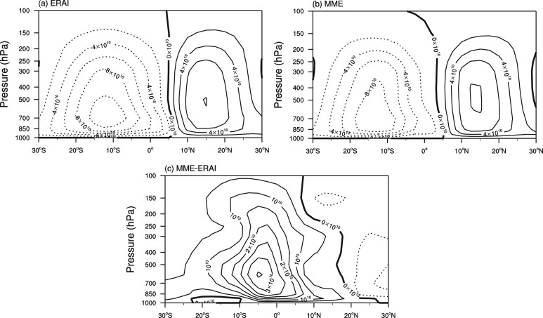
Fig. 1 shows the annual mean climatology of MSF derived from MME, ERAI, and the differences between MME and ERAI. Fig. 1 a and 1 b shows that the spatial structure of MSF derived from MME and ERAI, the two datasets are consistent, with one cell in each hemisphere. The southern cell is slightly stronger than the northern one and the southern cell extends to the northern hemisphere at about 7°N, which corresponds to the location of the intertropical convergence zone (ITCZ). The descending branches of the two cells locate at about 30°S and 30°N, respectively. In spite of the consistent spatial structure of MSF, the magnitude of MSF derived from MME is weaker than that from ERAI in both southern and northern cells (Fig. 1 c). The weak bias is especially obvious in the southern cell.

Fig. 1. Climatology of annual mean mass stream function (MSF) from (a) ECMWF Re-Analysis (ERAI), (b) multi-model ensemble mean (MME), and (c) the difference of MME (unit: kg s−1 ).

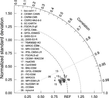
The performance of each model in simulating the climatology of the annual mean HC is further evaluated with the Taylor diagram shown in Fig. 2 . Except for GFDL-CM3, GISS-E2-H and MIROC-ESM, the strength of the climatological HC of the remaining models are weaker than that of the ERAI. The models have high pattern correlations with ERAI (r  > 0.9), except MRI-CGCM3, indicating that the models have good performance in simulating the spatial structure of the climatology of annual mean HC. But most models underestimated the intensity of the annual mean HC, except for GISS-E2-H and FIO-ESM which perform well in simulating both the structure and intensity. In general, the CMIP5 models can simulate the climatology of the annual mean HC properly, but with weak bias in southern hemisphere.

Fig. 2. Taylor diagram for annual mean mass stream function (MSF).

3.2. Spatial structure of the principal modes of the annual mean HC

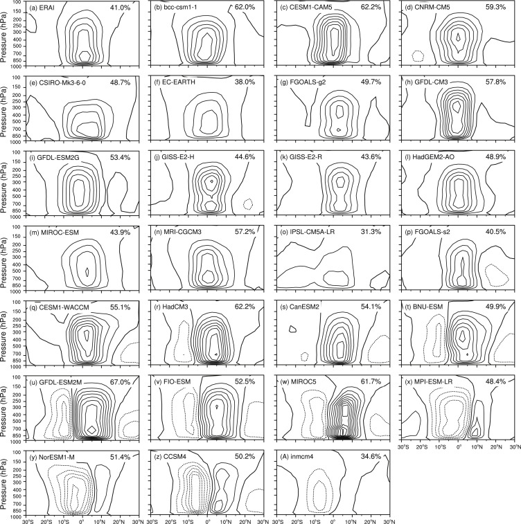
Here, the spatial structure simulated by the models is mainly focused on. Fig. 3 shows the EOF1 of the annual mean HC from ERAI and the 26 CMIP5 models. The EOF1 of the annual mean HC derived from ERAI presents AM, with ascending (descending) motion at 10°S (10°N). Most models can generally simulate the AM, which is similar to that from the ERAI. But there are 8 models (BNU-ESM, GFDL-ESM2M, FIO-ESM, MIROCS, MPI-ESM-LR, NorESM1M, CCSM4 and inmcm4) having different results, which not only have a cross-equatorial cell, but also a relatively weak cell accompanying with the asymmetric cells. The EOF1 of CCSM4 shows approximately a SM. The explained variance of ERAI is 41.0%, but the models range from 31.3% to 67.0%. Additionally, the EOF1 of IPSL-CM5A-LR has a cross-equatorial cell extending to 30°S, which is much wider than ERAI.

Fig. 3. EOF1 of annual mean mass stream function (MSF) from (a) ECMWF Re-Analysis (ERAI), and (b–A) each model for the period of 1979–2005. The contour intervals are 2 × 109  kg s−1 . The solid (dashed) contours indicate the positive (negative) values. The value at the top-right corner of each figure is the explained variance to the total for each dataset.

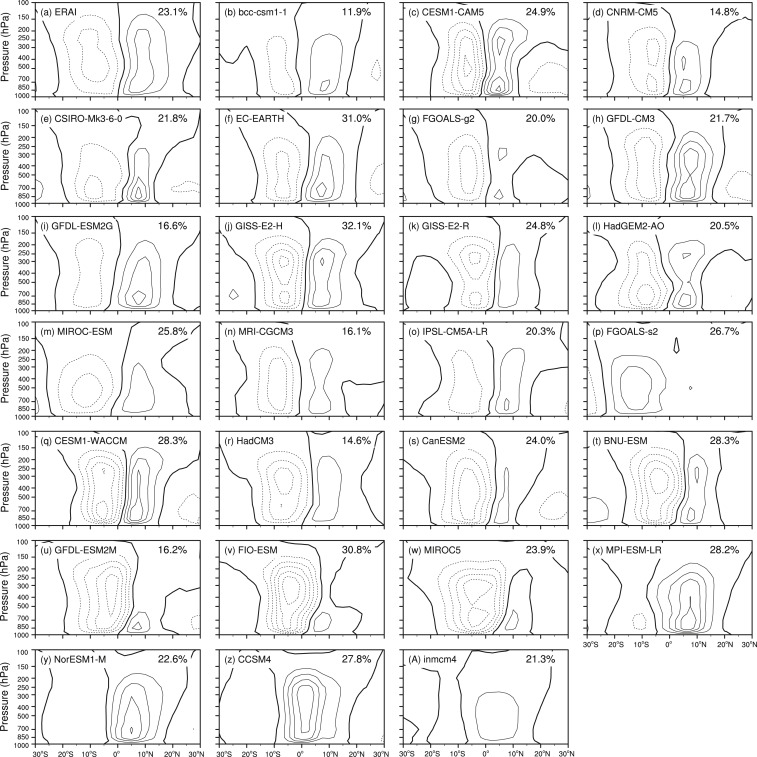
Fig. 4 shows the EOF2 of the annual mean HC from ERAI and the models. The EOF2 of ERAI presents SM, with two comparable cells in different signs on the flanks of the equator. They share the same upward branch at the equator, but with descending branches at 20°S and 20°N, respectively. Most models can present such spatial structure for their EOF2, but the 8 models mentioned above still have differences. For BNU-ESM, GFDL-ESM2M, FIO-ESM and MIROC5, the southern cells extend to the northern hemisphere. For MPI-ESM-LR, NorESM1-M, CCSM4 and inmcm4, they only have a strong cross-equatorial cell. The results indicate that for EOF2, ERAI and most models shows symmetric structure, while the 8 models shows asymmetric structure. Noting that the model FGOALS-s2 shows a single cell in the southern hemisphere, which is different from both AM and SM.

Fig. 4. Same as Fig. 3 , but for EOF2.

Except for the spatial structures of the principal modes, the associated time series is another important aspect of the interannual variability. The time series of the first two principal modes of models were also compared with ERAI. The results show that all of the CMIP5 models have weak correlations with observation (r  < 0.3). This indicates that the CMIP5 models have weak ability to reproduce a consistent temporal evolution of the principal modes with the observation. However, as another aspect of the interannual variability, the spatial structure of the principal mode can be well captured by most of the CMIP5 models.

In order to evaluate how well each model simulate the AM and SM, Table 2 lists the pattern correlation coefficients of the principal modes between ERAI and models. It can be seen from Fig. 3  and Fig. 4 and Table 2 that the pattern correlation coefficients above 0.7 indicate good simulations of the spatial structures. Eighteen out of the 26 models have high pattern correlations with the observations indicating that these models can properly reproduce both AM and SM. IPSL-CM5A-LR can reproduce SM properly, but shows poor simulation of AM. On the contrary, FGOALS-s2 can reproduce AM, but cannot reproduce SM. The remaining 4 models (FIO-ESM, MIROC5, MPI-ESM-LR, NorESM1-M) will not be discussed because that the difference between r_{(EOF1, AM)} and r_{(EOF2, AM)} of these models are small, and it is the same case for r_{(EOF1, SM)} and r_{(EOF2, SM)} . This implies that the EOF1 and EOF2 are hard to distinguish among these models. The last two models, CCSM4 and inmcm4, simulate a reversed sequence of AM and SM, i.e., the EOF1s of the annual mean HC in these two models are SM and EOF2s of the annual mean HC are AM.

Table 2. Pattern correlation coefficients of leading modes between model and observation during the period of 1979–2005.

Category	Model	r(EOF1, AM)	r(EOF2, SM)	r(EOF2, AM)	r(EOF1, SM)
Group A	bcc-csm1-1	0.94a	0.81a	0.17	0.25
	CESM1-CAM5	0.96a	0.75a	0.25	0.06
	CNRM-CM5	0.96a	0.82a	0.18	0.01
	CSIRO-Mk3-6-0	0.87a	0.78a	0.01	0.23
	EC-EARTH	0.93a	0.87a	0.03	0.09
	FGOALS-g2	0.92a	0.75a	0.02	0.30
	GFDL-CM3	0.92a	0.87a	0.26	0.21
	GFDL-ESM2G	0.89a	0.89a	0.29	0.37
	GISS-E2-H	0.94a	0.9a	0.03	0.13
	GISS-E2-R	0.83a	0.71a	0.36	0.52
	HadGEM2-AO	0.97a	0.74a	0.31	0.02
	MIROC-ESM	0.94a	0.87a	0.21	0.12
	MRI-CGCM3	0.97a	0.86a	0.24	0.03
	CESM1-WACCM	0.93a	0.82a	0.03	0.29
	HadCM3	0.89a	0.88a	0.08	0.13
	CanESM2	0.91a	0.81a	0.16	0.23
	BNU-ESM	0.78a	0.75a	0.19	0.39
	GFDL-ESM2M	0.73a	0.72a	0.14	0.37
Group B	CCSM4	0.11	0.23	0.93a	0.86a
	inmcm4	0.15	0.44	0.82a	0.75a
Group C	IPSL-CM5A-LR	0.66	0.86a	0.38	0.57
	FGOALS-s2	0.95a	0.5	0.44	0.65
	FIO-ESM	0.65	0.61	0.58	0.69
	MIROC5	0.56	0.6	0.69	0.68
	MPI-ESM-LR	0.64	0.67	0.62	0.62
	NorESM1-M	0.60	0.65	0.67	0.69

a. Indicates the values larger than 0.7.

According to the above results, all the models are grouped into 3 categories: Group A (bcc-csm1-1, CESM1-CAM5, CNRM-CM5, CSIRO-Mk3-6-0, EC-EARTH, FGOALS-g2, GFDL-CM3, GFDL-ESM2G, GISS-E2-H, GISS-E2-R, HadGEM2-AO, MIROC-ESM, MRI-CGCM3, CESM1-WACCM, HadCM3, CanESM2, BNU-ESM, GFDL-ESM2M) can properly reproduce both AM and SM; Group B (IPSL-CM5A-LR, FGOALS-s2) can only reproduce one of AM or SM; Group C (CCSM4, inmcm4) simulated reversed sequence of AM and SM.

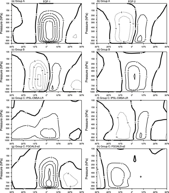
Fig. 5 shows the first two principal modes of each group. The spatial structure of EOF1 and EOF2 from Group A has good consistency with those from ERAI, but the strength is relatively weaker than ERAI (Fig. 3  and Fig. 4 a). For Group B, EOF1 shows SM with southern cell stronger than northern cell and EOF2 shows AM. For Group C, the IPSL-CM5A-LR can only reproduce the SM as EOF2, while the EOF1 shows a cross-equatorial cell, which is too large compared with observation. The FGOALS-s2 can only simulate the AM in EOF1, the EOF2 shows a single cell in the southern Hemisphere unlike neither AM nor SM.

Fig. 5. The (a) first and (b) second principal modes of the annual mean Hadley circulation variability from multi-model ensemble mean of Group A during 1979–2005. (c)–(d) for multi-model ensemble mean of Group B. (e)–(f) as in (a)–(b), but for IPSL-CM5A-LR in Group C. (g)–(h) for FGOALS-s2 in Group C. The contour intervals are 2 × 109  kg s−1 . The solid (dashed) contours indicate the positive (negative) values.

3.3. Relationship between the principal modes and the tropical SST

The tropical circulation has been proved to be closely related to the SST structure (Feng and Li, 2013  and Hu et al., 2014 ). Previous studies also documented that the AM is caused by asymmetric SSTA and SM is caused by symmetric SSTA (Feng et al., 2013  and Feng and Li, 2013 ). How this relationship works in CMIP5 models is an interesting question. The time series (PC) of AM and SM will be used to regress the zonal mean SSTA, thus, the corresponding SST structure can be observed.

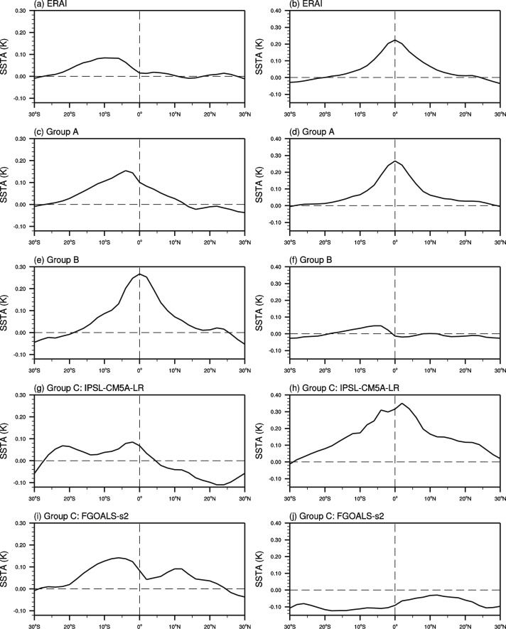
Fig. 6 shows the regressed zonal mean SSTA by PC1 and PC2 of the reanalysis data and models. For ERAI and Group A, PC1 regressed SSTA presents a peak value at 10°S and 5°S (Fig. 6 a and c), respectively, leading to asymmetric thermal forcing and thus AM. The PC2 regressed SSTA shows symmetric pattern with peak values at the equator, which can lead to symmetric thermal forcing and SM occurrence. For Group B, the PC1 regressed SSTA shows symmetric pattern while the PC2 regressed SSTA shows asymmetric pattern, which may be the reason why it simulates a reversed sequence of AM and SM compared with the observation. For IPSL-CM5A-LR in Group C, the PC2 of regressed SSTA shows similar pattern as in ERAI and Group A, thus it can simulate well the SM. But the PC1 regressed SSTA is flat in the southern hemisphere, which may be related to the wide latitudinal range of the cross-equatorial cell structure (Fig. 5 c). And it also shows negative SSTA in northern hemisphere which is different from the near zero values in observation. For FGOALS-s2 in Group C, the PC1 regressed SSTA is similar to ERAI and Group A, thus it can simulate the AM, while the poor simulation of PC2 regressed SSTA may leads to the poor simulation of SM.

Fig. 6. The time series of the (a) first and (b) second principal modes regressed zonal mean SSTA based on ECMWF Re-Analysis (ERAI) during the period of 1979–2005. (c–d) for Group A and B, respectively. (g–h) and (i–j) for IPSL-CM5A-LR and FGOALS-s2, respectively.

Fig. 7 shows the relationship between the principal modes' strength (represented by PC of each modes) and the meridional SST gradient index. The meridional symmetric SST index (MSSI) and the meridional asymmetric SST index (MASI) are defined as (Feng and Li, 2013 ):

$MSSI={\overline {SSTA}}_{\left[5{\mbox{°}}S-5{\mbox{°}}N\right]}-$$0.5\cdot {\overline {SSTA}}_{\left[5{\mbox{°}}N-15{\mbox{°}}N\right]}-$$0.5\cdot {\overline {SSTA}}_{[15{\mbox{°}}S-5{\mbox{°}}S],}$

( 1)

$MASI={\overline {SST}}_{\left[5{\mbox{°}}N-15{\mbox{°}}N\right]}-$${\overline {SST}}_{[15{\mbox{°}}S-5{\mbox{°}}S],}$

( 2)

where the overbars denote zonal mean and square brackets denote the latitudes where average is performed.

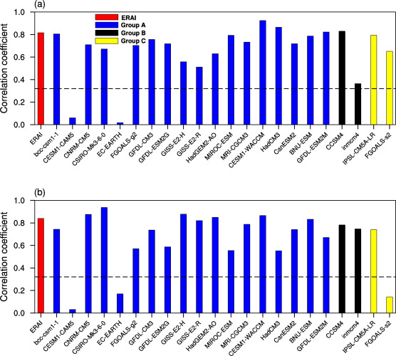
Fig. 7. Correlation coefficients between the time series of (a) asymmetric mode (AM) and the asymmetric sea surface temperature (SST) index during 1979–2005, (b) for correlation coefficients between symmetric mode (SM) and symmetric SST index. The dashed line indicates the 90% confidence level.

Only the models in the 3 categories were considered. It can be seen that except for CESM-CAM5 and EC_EARTH, all the models shows high correlation coefficients between the variabilities of AM and the asymmetric SST component, which is consistent with the observation (Fig. 7 a). For SM, all the models, except CESM-CAM5, EC-EARTH and FGOALS-s2, have high correlation coefficients between variabilities of SM and the symmetric SST component, which is also consistent with observation (Fig. 7 b). Note that although CESM-CAM5 and EC_EARTH in Group A have good simulation of the AM or SM spatial structure, they have weak ability in reflecting the circulation response to the SST gradient forcing.

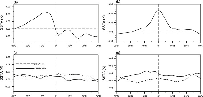
Further, how well each model performs in simulating the variability of meridional SST gradient itself has not been recognized. It is possible that CESM-CAM5 and EC-EARTH have poor simulation of the SST structure corresponds to AM and SM. Fig. 8 shows the PC1 and PC2 regressed zonal mean SSTA based Group A excluding CESM-CAM5 and EC-EARTH. PC1 regressed SST in Group A shows the peak value closer to the equator than observation and has larger cross-equatorial SST gradient (Fig. 6 a and c). When excluding the CESM-CAM5 and EC-EARTH, the regressed SST peak value is more approaching to that of observation and the cross-equatorial SST gradient is also more consistent with the observation (Fig. 8 a). For PC2 regressed SSTA, there is no big change before and after excluding the two models (Fig. 6  and Fig. 8 b). When observed independently, the two models show no asymmetric and symmetric structure for PC1 and PC2 regressed zonal mean SSTA. Instead, PC1 regressed SSTA for both models and PC2 regressed SSTA for EC-EARTH present homogenous warming in the tropics, and PC2 regressed SSTA present asymmetric distribution (Fig. 8 c and d). It implies that although the two models simulate properly the AM and SM, but do not properly simulate the SST structure corresponding to the principal modes.

Fig. 8. (a–b) as in Fig. 6 (a–b), respectively, but for Group A excluding CESM-CAM5 and EC-EARTH. (c–d) for CESM-CAM5 (solid line) and EC-EARTH (dashed line).

4. Discussion and conclusions

In this paper, the climatology and interannual variability of the annual mean HC by using 26 climate models from CMIP5 are analyzed. The results show that most models perform well in simulating the spatial structure of the annual mean climatology of the HC, but the strengths of HC in most models are weaker than the observation. Eighteen of the CMIP5 models in Group A (Table 2 ) can simulate both the AM and SM well. The CCSM4 and inmcm4 present a reversed sequence of AM and SM, i.e., EOF1 shows SM-like spatial structure while EOF2 shows AM-like spatial structure. IPSL-CM5A-LR can only reproduce SM and FGOALS-s2 can only reproduce AM properly. The rest of the models can simulate neither AM nor SM. All the models have relatively weak ability in simulation of the time evolution of the AM and SM, the correlation coefficients with observation are less than 0.3.

Further analysis shows that the symmetry of the HC principal modes has close relationship with the symmetry of the zonal mean SSTA, i.e., the symmetric (asymmetric) SSTA corresponds to the SM (AM). Some models do not properly simulate AM and SM, this is possibly because these models cannot simulate SSTA structure properly. Most models have good response to the meridional SST gradient, even if some models do not properly simulated the SST structure. On the other hand, some models properly simulated the principal modes, but do not properly simulate the corresponding SST structure. Therefore, these models should be taken more care when classify the models into groups.

The results provide clues that why some models have larger explained variance of SM than AM. It is possibly because that the models with SM for EOF1 have larger variance of symmetric SSTA than asymmetric SSTA. Also, not properly simulating either symmetric or asymmetric SSTA will lead to the decrease of the ability in simulating SM or AM as in Group C.

The current study draws the attention to the model performance in simulating both the HC principal modes and their relationship with the air–sea coupling processes. More studies needs to be carried out to investigate why some models do not properly simulate the SST structure and its relationship with the HC principal modes. These works can help the models to gain higher scores in the climate projection, because the HC is key to the climate system changes.

Acknowledgments

This work was supported by the National Natural Science Foundation of China (41530424 and 41475076 ).

References

1. Chen et al., 2002 J.Y. Chen, B.E. Carlson, A.D. Genio; Evidence for strengthening of the tropical general circulation in the 1990s; Science, 295 (2002), pp. 838–841
2. Dee et al., 2011 D.P. Dee, S.M. Uppala, A.J. Simmons, et al.; The ERA-interim reanalysis: configuration and performance of the data assimilation system; Q. J. R. Meteorol. Soc., 137 (2011), pp. 553–597
3. Dima and Wallace, 2003 I.M. Dima, J.M. Wallace; On the seasonality of the Hadley cell; J. Atmos. Sci., 60 (2003), pp. 1522–1527
4. Feng et al., 2011 R. Feng, J.-P. Li, J.C. Wang; Regime change of the boreal summer Hadley circulation and its connection with the tropical SST; J. Clim., 24 (2011), pp. 3867–3877
5. Feng et al., 2013 J. Feng, J.-P. Li, F. Xie; Long-term variation of the principal mode of boreal spring Hadley circulation linked to SST over the Indo-Pacific warm pool; J. Clim., 26 (2013), pp. 532–544
6. Feng and Li, 2013 J. Feng, J.-P. Li; Contrasting impacts of two types of ENSO on the boreal spring Hadley circulation; J. Clim., 26 (2013), pp. 4773–4789
7. Feng et al., 2015 J. Feng, J.-P. Li, J.-L. Zhu, et al.; Simulation of the equatorially asymmetric mode of the Hadley circulation in CMIP5 models; Adv. Atmos. Sci., 32 (8) (2015), pp. 1129–1142
8. Frierson et al., 2007 D.M.W. Frierson, J. Lu, G. Chen; Width of the Hadley cell in simple and comprehensive general circulation models; Geophys. Res. Lett., 34 (18) (2007), p. L18804
9. Fu et al., 2006 Q. Fu, C.M. Johanson, J.M. Wallace, et al.; Enhanced mid-latitude tropospheric warming in satellite measurements; Science, 312 (2006), p. 1179
10. Holton, 1992 J.R. Holton; An Introduction to Dynamic Meteorology; (third ed.)Academic Press San Diego, Calif (1992)
11. Hou, 1998 A.Y. Hou; Hadley circulation as a modulator of the extratropical climate; J. Clim., 55 (1998), pp. 2437–2457
12. Hu et al., 2014 D.-Z. Hu, W.-S. Tian, F. Xie, et al.; Effects of meridional sea surface temperature changes on stratospheric temperature and circulation; Adv. Atmos. Sci., 31 (2014), pp. 1–13
13. Hu and Fu, 2007 Y.-Y. Hu, Q. Fu; Observed poleward expansion of the Hadley circulation since 1979; Atmos. Chem. Phys., 7 (2007), pp. 5229–5236
14. Hu et al., 2011 Y.-Y. Hu, C. Zhou, J.-P. Liu; Observational evidence for poleward expansion of the Hadley circulation; Adv. Atmos. Sci., 28 (1) (2011), pp. 33–44
15. Hu et al., 2013 Y.-Y. Hu, L.-J. Tao, J.-P. Liu; Poleward expansion of the Hadley circulation in CMIP5 simulations; Adv. Atmos. Sci., 30 (3) (2013), pp. 790–795
16. Johanson and Fu, 2009 C.M. Johanson, Q. Fu; Hadley cell widening: model simulations versus observations; J. Clim., 22 (2009), pp. 2713–2725
17. Li, 2001 J.-P. Li; Atlas of Climate of Global Atmospheric Circulation I; China Meteorology Press, Beijing (2001) (in Chinese)
18. Li et al., 2013 J.-P. Li, R.-C. Ren, Y.-Q. Qi, et al.; Progress in air–land–sea interactions in Asia and their role in global and Asian climate change; Chin. J. Atmos. Sci., 37 (2) (2013), pp. 518–538 (in Chinese)
19. Li et al., 2015 X.-F. Li, J.-P. Li, Y. Li; Recent winter precipitation increase in the middle–lower Yangtze River Valley since the late 1970s: a response to warming in the tropical Indian Ocean; J. Clim., 28 (2015), pp. 3857–3879
20. Lu et al., 2007 J. Lu, G.A. Vecchi, T. Reichler; Expansion of the Hadley cell under global warming; Geophys. Res. Lett., 34 (2007), p. L06805
21. Ma and Li, 2007 J. Ma, J.-P. Li; Strengthening of the boreal winter Hadley circulation and its connection with ENSO; Prog. Nat. Sci., 17 (2007), pp. 1327–1333
22. Ma and Li, 2008 J. Ma, J.-P. Li; The principal modes of variability of the boreal winter Hadley cell; Geophys. Res. Lett., 35 (2008), p. L01808
23. Mitas and Clement, 2005 C.M. Mitas, A. Clement; Has the Hadley cell been strengthening in recent decades?; Geophys. Res. Lett., 32 (2005), p. L03809
24. Mitas and Clement, 2006 C.M. Mitas, A. Clement; Recent behavior of the Hadley cell and tropical thermodynamics in climate models and reanalyses; Geophys. Res. Lett., 33 (2006), p. L01810
25. Nguyen et al., 2013 H. Nguyen, A. Evans, C. Lucas, et al.; The Hadley circulation in reanalyses: climatology, variability, and change; J. Clim., 26 (2013), pp. 3357–3376
26. Polvani et al., 2011 L.M. Polvani, D.W. Waugh, G.J.P. Correa, et al.; Stratospheric ozone depletion: the main driver of 20th century atmospheric circulation changes in the Southern Hemisphere; J. Clim., 24 (2011), pp. 795–812
27. Quan et al., 2004 X.-W. Quan, H.F. Diaz, M.P. Hoerling; Change in the tropical Hadley cell since 1950; H.F. Diaz, R.S. Bradley (Eds.), The Hadley Circulation: Past, Present, and Future, Cambridge University Press, Cambridge (2004), pp. 85–120
28. Quan et al., 2014 X.W. Quan, M.P. Hoerling, J. Perlwitz, et al.; How fast are the tropics expanding?; J. Clim., 27 (2014), pp. 1999–2013
29. Schneider et al., 2010 T. Schneider, P.A. O'Gorman, X.J. Levine; Water vapor and the dynamics of climate changes; Rev. Geophys., 48 (2010), p. RG3001
30. Seidel et al., 2008 D.J. Seidel, Q. Fu, W.J. Randel, et al.; Widening of the tropical belt in a changing climate; Nat. Geosci., 1 (2008), pp. 21–24
31. Smith et al., 2008 T.M. Smith, R.W. Reynolds, T.C. Peterson, et al.; Improvements NOAAs historical merged land-ocean temp analysis (1880–2006); J. Clim., 21 (2008), pp. 2283–2296
32. Stachnik and Schumacher, 2011 J.P. Stachnik, C. Schumacher; A comparison of the Hadley circulation in modern reanalyses; J. Geophys. Res., 116 (2011), p. D22102
33. Tanaka et al., 2004 H.L. Tanaka, N. Ishizaki, A. Kitoh; Trend and interannual variability of Walker, monsoon and Hadley circulations defined by velocity potential in the upper troposphere; Tellus, 56A (2004), pp. 250–269
34. Taylor et al., 2012 K.E. Taylor, R.J. Stouffer, G.A. Meehl; An overview of CMIP5 and the experiment design; Bull. Am. Meteorol. Soc., 93 (2012), pp. 485–498
35. Wielicki et al., 2002 B.A. Wielicki, T. Wong, R.P. Allan, et al.; Evidence for large decadal variability in the tropical mean radiative energy budget; Science, 295 (2002), pp. 841–843
36. Zhang and Wang, 2013 G. Zhang, Z. Wang; Interannual variability of the Atlantic Hadley circulation in boreal summer and its impacts on tropical cyclone activity; J. Clim., 26 (2013), pp. 8529–8544
37. Zhang and Wang, 2015 G. Zhang, Z. Wang; Interannual variability of tropical cyclone activity and regional Hadley circulation over the Northeastern Pacific; Geophys. Res. Lett., 42 (2015), pp. 2473–2481