Offshore wind energy potential estimation using UPSCALE climate data

Abstract

Offshore and near-shore wind energy is one of the major renewable energy resources, which already make a substantial contribution to the energy supply in Europe. Nevertheless, development is still in the start-up phase, with new projects being planned and implemented continuously. This development needs to be informed, to enable deployment at the most suitable/ideal locations. However, in order to predict the potential energy yield, forecasts have to be made. In this paper the authors present a scoping study. This study uses high-resolution climate data to predict wind speeds at various heights, and various locations along the coast of Mexico. Several techniques for wind extrapolation are explored, alongside a new method based on data analysis. The results show clearly a strong sensitivity to the method chosen, and results have to be interpreted accordingly. Also, the impact of water vapor is shown, using a method that predicts the moist air density at the hub height. The paper indicates that valuable information can be gained from the analyses undertaken, prior to embarking on detailed, targeted studies. The paper concludes with recommendations for further work.

Introduction

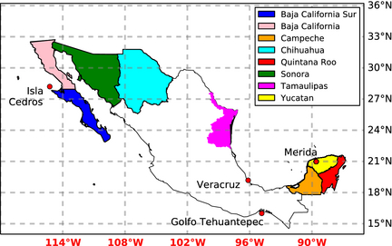
Prior to micrositing campaigns, which estimate the potential of wind energy resources, and proposals for development that follow, likely sites of interest have to be identified. This has to be informed from the country-wide scale down to the local scale. At the local scale, in particular if complex orography is present, high-resolution models are required, sometimes even requiring 3d turbulence models (cf. [1]). However, this analysis is costly and prior to this available data sources have to be exhausted to inform these campaigns. To date no systematic and complete analysis for Mexico has been performed. Individual studies exist, driven by individual local interests. The National Renewable Energy Laboratory (NREL) lists eight areas for Mexico, an atlas for Oaxaca and individual maps for Baja California (north and south), western Chihuahua, northwestern Mexico, Sonora (east and west) and Quintana Roo and Yucatan. Refer to Figure 1 for these and other locations referred to in this paper. However, together these only represent three continuous and distinct geographic areas and do not include resource assessments at offshore sites (a few include a near coastal area).

Figure 1. Map indicating geographic locations referred to in this study.

In this work, data from one of the largest global climate simulation initiatives to date were analyzed to assess offshore wind energy potential around Mexico. Using a global climate simulation has the advantage that the energy yield resulting from the analysis is comparable for all regions of interest, that is self-consistent. Furthermore, climatologically correct data are available, even at locations which have a low density of observations. There is of course a limit to which data that is climatology correct can be relied on as being accurate. Most noteworthy in this respect is probably the large wind bias found in the North American Regional Reanalysis (NARR) data when compared to the observational North American Monsoon Experiment (NAME) data set. A reanalysis, such as the NARR data, would be assumed to be closer to observations as it is constrained to observations. Nevertheless a wind bias can be found, cf. [2]. It is more difficult to assess an unconstrained data set, such as the upscale data set. Single temporal meteorological events, such as the Gulf surge, a northward surge of cold air along the Gulf of California, for example, may occur at different times. A one-to-one comparison would then show up two failures, one when the surge was observed, but did not occur in the model, and another when the surge eventually occurred in the model, but was not observed (because it had already passed). To be climatologically correct the surges have to occur at roughly the correct rate. However, they do not have to occur at the same time. A further disadvantage is that the output is usually highly compressed, using time and domain profiles which sample the whole data set at discrete locations (often pressure levels at full horizontal resolution) and apply time averaging. For all grid points in the region considered here the data were analyzed with respect to 10 m wind speed histogram, direction histogram, vertical velocity/air density distribution, and wind power density.

The Data Source

For this paper the main data source is the global N512 (512 is the number of two grid length waves that can be supported in the EW direction, hence N512 yields 1024 × 768 grid points EWxNS) UPSCALE data set, based on the HadGEM3-GA3.0 configuration of the Met Office Unified Model (MetUM) version 8.0, combined with the GL3.0 configuration of the JULES community land surface model, as documented in [3]. The model was configured to reproduce the present climate for the period February 1985 to December 2011. More detailed information about the UPSCALE model simulations is available in [4, 5]. The HadGEM model has a proven track record in the area, in particular for local climate features such as Mid Summer Drought and Great Plains low-level jet, for example (cf. [6, 7]). Furthermore, in the results presented here are compared to the NREL results, where available, as a means of validation.

Analysis

A complication with using climate data is the fact that the output is sparse, in space and time. This has been improved in this data set markedly, previously cell sizes where in the order of 125 km [8] or 80 km [9], and not 25 as in this data set (or for example CMIP5: HadGEM-CC which was run at N96). However, not all model levels are stored during the run and not all time steps are available for retrospective analysis. From this data set the 10 m wind speeds are available as daily means, 6 h maximum, daily max wind speed, daily mean components and three hourly instantaneous components. Additionally restart dumps are available. These contain all model variables at full model resolution for 30 discrete points in time, distributed over the analysis period. These 30 points in time are on the 1st of March of every year, starting in 1985, using a 360 day calendar. Therefore, seasonal variation (or even decadal variation) cannot be included in the derivation of the height extrapolation coefficients (see Section 'Wind speed' below). In the vertical the dumps contain 85 levels for “ρ points”, that is where density, pressure and velocity are stored, and 86 “θ levels”, that is where potential temperature and moisture are stored, frequently referred to as Charney–Phillips grid [10]. The first four heights (over sea) are listed in Table 1.

Table 1. Vertical resolution above sea [m].

θ points	ρ points
20.0	10
53.3	36.7
100.0	76.7
160.0	130

In the vertical, in the climate data set, either the 10 m or pressure coordinates wind speed are available. However, the first pressure coordinate (aside from 1000 hPa) is 925 hPa, approximately 750 m, which is much higher than useful for wind energy resource exploitation. This means that in the vertical the wind speeds have to be extrapolated. This extrapolation can be then tested against the 30 available full model level profiles, as shown below. Furthermore, the air density needs to be evaluated, extrapolated and tested in the same fashion.

Air density

From the 30 vertical profiles, a representative vertical structure for air density can be derived, using (cf. equation 42 in [11])

${\rho }_{dry}=p_{o}{\frac {{\overline {\pi }}^{\frac {1-\kappa }{\kappa }}}{R{\theta }_{\upsilon }}},$

(1)

${\rho }_{wet}={\rho }_{dry}\left(1+m\right),$

(2)

and

$\kappa ={\frac {R}{c_{p}}},$

(3)

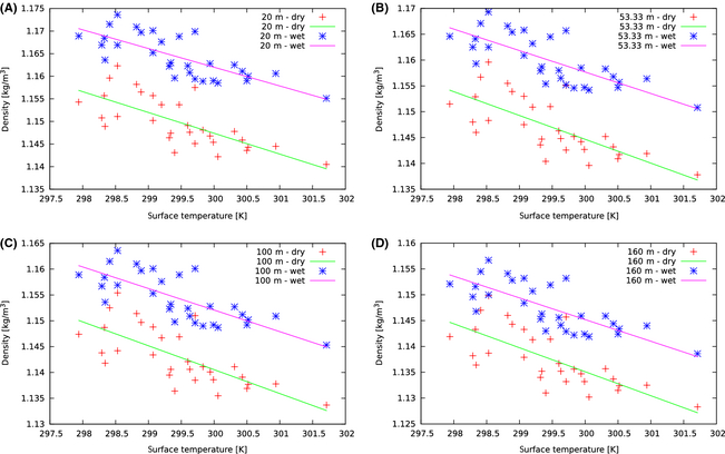
where the constants p₀, R, and c_p, denote the surface reference pressure, gas constant and specific heat capacity, and the spatially (3D) and temporally varying variables π, θ_v and m denote Exner pressure (point wise vertically averaged onto the location of θ, because in this model θ_v is staggered vertically with respect to π, that is not on the same height – hence the bar), dry virtual temperature and mixing ratio, respectively. Linear regression is applied to these data at discrete heights, as shown in Figure 2, yielding the coefficients a_h and b_h – one set of coefficients for each horizontal grid point analyzed according to

${\rho }_{wet}\left(z=h\right)=a_{h}T_{s}+b_{h},$

(4)

Figure 2. Comparison of the 30 model values for air density versus the linear regression (Equation (4)) and the four lowest discrete model levels for the first grid point (see Section 'Wind speed'). (A) at 20 m (B) at 53.33 m (C) at 100 m (D) at 160 m.

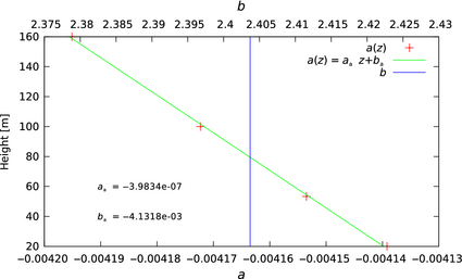
where T_s denotes the model surface temperature. The coefficients a_h and b_h can then be further approximated with respect to height as

$a_{h}\left(z\right)=a_{a}z+b_{a}\quad {\mbox{and}}\quad b_{h}\equiv {\mbox{const}},$

(5)

as shown in Figure 3.

Figure 3. Regression of the coefficients of the linear equation for wet air density.

The quality of the regression can potentially be enhanced by using more data points from the surrounding area or even the whole domain. A shortcoming is that these are only representative data for 30 days. Therefore, seasonal variation is not included. However, in first order the air density depends on temperature, and close to the ocean this air temperature depends closely on the surface temperature and the vertical moisture distribution. As neither air density, pressure, temperature nor humidity are available in the data set (at sufficient resolution) this is probably an acceptable compromise, especially considering that the air density variation is around 3% and only contributes linearly to the WPD. Nevertheless, a clear and systematic difference between wet and dry air density can be observed, of roughly 2.5%. Figure 2 clearly emphasizes the importance of moisture in the estimation of air density.

Wind speed

In order to estimate the velocities at different heights (rarely are turbines situated at 10 m) a power law relationship

${\frac {u}{u_{r}}}=({\frac {z}{z_{r}}})^{\alpha },$

(6)

is frequently used, where u represents the wind speed (in meters per second) at height z (in meters), and u_r is the known wind speed at a reference height z_r, respectively. The exponent α is an empirically derived coefficient, frequently taken as 1/7 [12], but other sources (for example [13]) quote 0.11 to be a better choice over open water. More complex estimations could be made, if the surface roughness length and the vertical Monin-Obukhov stability function were known. However, this is usually not the case. [12] suggest a different method to compute α when the wind profile is known:

$\alpha ={\frac {log{\frac {u_{r}}{u}}}{log{\frac {z_{r}}{z}}}}$

(7)

Here, z was chosen at 36.7 m and z_r at 76.7 m, resulting from the aforementioned vertical grid (cf. Table 1). A fourth method, developed here, similar to the method used for air density, involves regressing the 30 known vertical profiles against the functional relationship

${\frac {u(z)}{u(10)}}={\left({\frac {z}{10}}+cz\right)}^{a+b/z}$

(8)

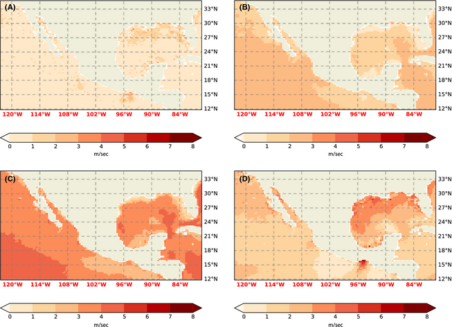
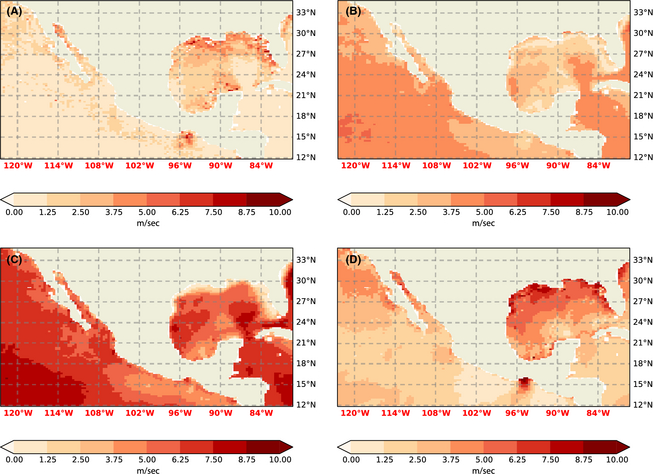
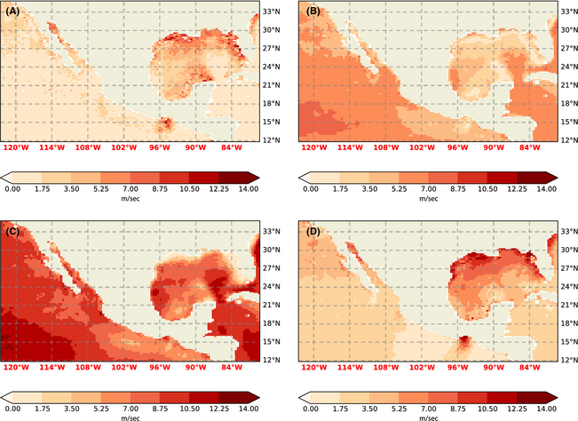
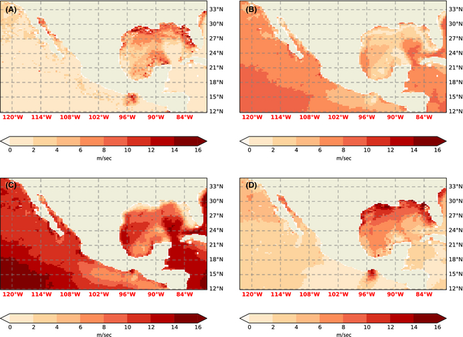
Since here instantaneous data at high vertical resolution are needed the main output of the climate model is not usable for the purpose of generating the extrapolation coefficients. Therefore, for this task the 30 restart dumps have to be used, which contain all vertical model levels, albeit at coarse (yearly) temporal resolution. The 10 m wind speed and surface temperature, which are used to compute the Wind Power Density, are available at high spatial and temporal resolution form the standard model output and hence include seasonal and decadal changes. The resulting coefficients a, b, and c are filtered, such that only those where b > 0 and c < 0 are used. The coefficients outside of these limits are unphysical results generated by profiles which first increase with height and then decrease. The velocities can then be reconstructed in the vertical using the average of these filtered coefficients. The obtained RMS errors (eq. (9)) for the first grid point (at latitude degrees north of 34.687 and longitude degrees east of 237.656), are presented in Table 2. Occasionally the above procedure is suboptimal, as can be seen in the plots in Figures 4-7 in the Gulf of México, for example. At the example of Figure 7 it can be seen how α = 0.11 is performing better in most parts of the Gulf and α = 1/7 is only preferable at the northern coast. Using eq. (8) has a clear advantage at the western coast and eastern mouth, even when compared to α = 0.11. Equation (7) has some advantage at the coast of Campeche and Yucatan. Therefore, for the results reproduced below, the equation with the lowest RMS error

$RMS={\sqrt {{\frac {1}{n}}\sum _{1}^{n}{\left(u-u_{est}\right)}^{2}}},$

(9)

Table 2. RMS error in vertical velocity reconstruction using the presented method with the resulting coefficients a = 4.854 × 10⁻² m, b = 0.942 m and c = −2.251 × 10⁻⁴ per m at the first grid point versus other popular choices using Equation (6).

Height	Equation (8)	α = 0.11	α = 1/7
10 m	0.0134 m/sec	0 m/sec	0 m/sec
36.67 m	0.1986 m/sec	2.3798 m/sec	4.4679 m/sec
76.67 m	0.3435 m/sec	4.6109 m/sec	8.2049 m/sec
130 m	0.2813 m/sec	6.8678 m/sec	11.7066 m/sec
196.66 m	0.1995 m/sec	9.1507 m/sec	15.0730 m/sec

Figure 4. RMS error (temporally meaned over the –30 data sets instantaneous wind – cf. Section 'Analysis') of wind extrapolation at 36.7 m. (A) Equation (8). (B) α = 0.11. (C) α = 1/7. (D) Equation (7).

Figure 5. RMS error (as in Fig. 4) of wind extrapolation at 76.7 m. (A) Equation (8). (B) α = 0.11. (C) α = 1/7. (D) Equation (7).

Figure 6. RMS error (as in Fig. 4) of wind extrapolation at 130 m. (A) Equation (8). (B) α = 0.11, (C): α = 1/7. (D) Equation (7).

Figure 7. RMS error (as in Fig. 4) of wind extrapolation at 196.7 m. (A) Equation (8). (B) α = 0.11. (C) α = 1/7. (D) Equation (7).

here defined as the absolute error, with u and u_est denoting wind in the model vertical profile and extrapolated wind, respectively, is chosen, on a gridpoint by gridpoint basis.

Wind speed histograms and wind power density

The wind speed histograms were binned using a 0.1 per ms bin and direction histograms using a 2π/100 radian bin width. Initially, the Wind Power Density, WPD, was computed assuming an air density of 1 kg m⁻³, as a proxy for not knowing the correct air density, that is

${\mbox{WPD}}={\frac {1}{2n}}\sum _{t=1}^{n}{\rho }_{t}{\mu }_{t}^{3}\quad \quad {\mbox{with}}\quad {\rho }_{t}\quad \equiv \quad 1\quad {\mbox{kg}}m^{-3},$

(10)

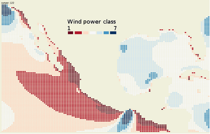
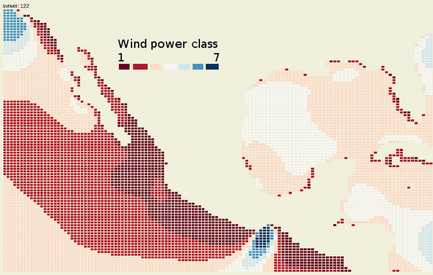
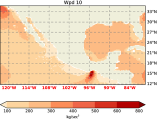
with n and t denoting the number of three hourly “measurements” (i.e., 79,440 samples covering the period 01/February/1985 to 1/September/2012 with a three hourly interval) and summation index, respectively. Unless otherwise noted 3 h instantaneous wind speed was used to compute the WPD, hence yielding a mean instantaneous wind power density, which, given sufficient samples, is reliable. The WPD class was then assigned using Table 3. The results are reproduced in Figures 8, 9. Then the extrapolated density ρ_wet, as derived above, was used to compute the Wind Power Density (Figure 10).

${\mbox{WPD}}={\frac {1}{2n}}\sum _{t=1}^{n}{\rho }_{wet}u^{3},$

(11)

Table 3. Wind energy class in Wm⁻².

Class	WPD10 m from	to WPD10 m
1	0	100
2	100	150
3	150	200
4	200	250
5	250	300
6	300	400
7	400	1000

Figure 8. Wind Power Class based on analysis using air density of 1 kg/m3 for the 10 m 6 h max wind speed. An output of the analysis is an online clickable map, providing straight forward access to the histograms and analysis results.

Figure 9. Wind Power Class based on analysis using air density of 1 kg/m3 for the 10 m 3 h instantaneous wind speed.

Figure 10. WPD with ρwet at 10 m.

where the subscript t indicating the summation of ρ and u is implied, for all remaining Figures. In Figure 8 the maximum wind speed over the 6 h period was used to derive the Wind Power Density, strictly a mean of the maximum wind power density. This quantity can serve as an absolute upper limit – that will not be achieved – as no further adjustment was made to accommodate the wind speed distribution.

Results and Discussion

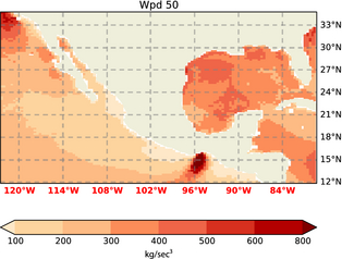
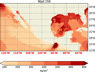
Comparing the panels in Figures 4-7 it is apparent that using α = 0.11 over sea is usually a better choice than the standard 1/7. However, the error can still be substantial, and better options clearly exist. Using a coefficient derived from two measurements, as proposed by [12], improves the predictions over open water, but still has significant error, even over such large water bodies as the Gulf of México. Also, in general, the Pacific and Atlantic coast as well as the eastern shore and mouth of the Gulf of México clearly benefit from the “ensemble fit” eq. (8), as presented in this paper. These errors (also when normalized by the mean wind speed) usually increase with height. This is due to two reasons: The mean wind speed increasing with height and a deviation from the log profile. The estimate of the climatological mean WPD in the Gulf of México depends crucially in the choice of extrapolation method used, as is obvious from the speckled coloring of the Gulf of México in Figures 11, 12. Obviously this caution does also need to be extended to studies that choose a constant method of extrapolation. There the uncertainty is even greater because it will not manifest itself the way it does here, in a highly spatially variable result.

Figure 11. WPD with ρwet at 50 m.

Figure 12. WPD with ρwet at 150 m.

Areas of interest

The results indicate six areas of special interest:

Upper Gulf of California

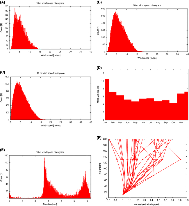
WPD from 300–400 W/m² at 50 m, increasing to 400–600 at 150 m can be reported here. The histograms in Figure 13 indicate strong directionality with two prevailing directions, Figure 13E, and only a moderate number of high wind occurrences Figure 13C. Despite the seasonal peak in January, Figure 13D, the monthly climatologies are similar, around 6 m/sec. Naturally uncertainty in this region is high, due to the orography and land sea contrast, which is not well resolved, even in this data set. A down scaling study will definitely be required here.

Figure 13. Upper Gulf of California. (A) Daily mean wind speed. (B) 6 h max wind speed. (C) Three hour instantaneous wind speed. (D) Monthly mean. (E) Wind direction (Northward wind is π rad, Eastward wind at 3/2π, Southward is 2π). (F) Vertical wind profile (normalized by 10 m wind speed).

North of Isla Cedros

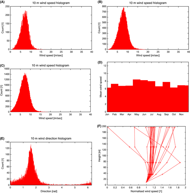
The predicted wind power density here is similar to the one in the Upper Gulf of California. However, the wind is mostly unidirectional, Figure 14E, significantly reduced seasonality, Figure 14D, and more symmetric distribution of high and low wind events Figure 14C.

Figure 14. North of Isla Cedros. (A) Daily mean wind speed. (B) 6 h max wind speed. (C) Three hour instantaneous wind speed. (D) Monthly mean. (E) Wind direction. (F) Vertical wind profile (normalized by 10 m wind speed).

Pacific coast of the northern part of Baja California Sur

Again, the histograms in Figure 15 are very similar to the ones for Isla Cedros, Figure 14, however notable here is the skew toward higher winds, Figure 15C.

Figure 15. Baja California Sur. (A) Daily mean wind speed. (B) 6 h max wind speed. (C) Three hour instantaneous wind speed. (D) Monthly mean. (E) Wind direction. (F) Vertical wind profile (normalized by 10 m wind speed).

Gulf of Tehuantepec

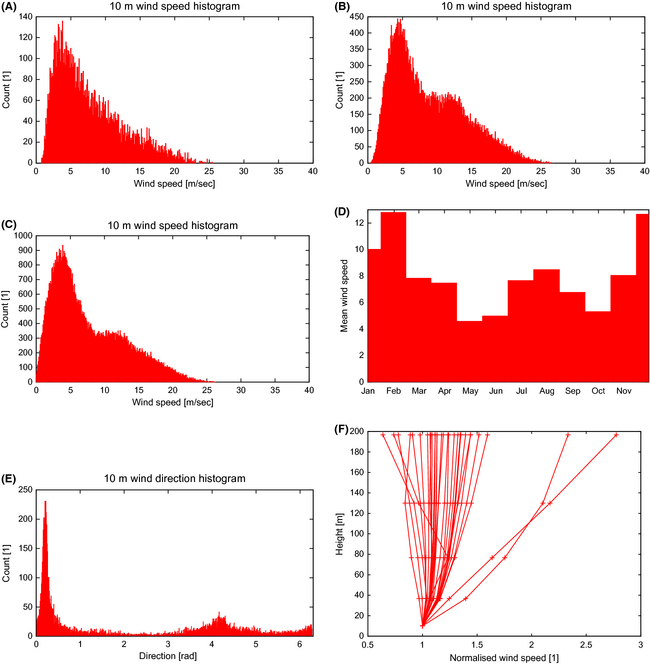
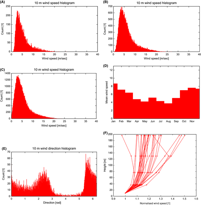
This region is often favored due to its prominence in wind energy density plots, promising yields in excess of 1000 W/m². Nevertheless the histograms indicate that, whilst the histogram peaks at roughly 5 m/sec, Figure 16C, there is a substantial high wind component, reaching up to 25 m/sec. Considering that here the unextrapolated 10 m winds are reported, the substantial technical challenges associated with harnessing these high and gusty winds that have a wide range of direction, Figure 16E, and have strong seasonality (4–12 m/sec), Figure 16D, should not be underestimated.

Figure 16. Gulf of Tehuantepec. (A) Daily mean wind speed. (B) 6 h max wind speed. (C) Three hour instantaneous wind speed. (D) Monthly mean. (E) Wind direction. (F) Vertical wind profile (normalized by 10 m wind speed).

Veracruz

Not as extreme as Gulf of Tehuantepec, but also showing some high wind gusts, change in directionality and substantial seasonal variation (4–8 m/sec), Figure 17C–E.

Figure 17. Veracruz. (A) Daily mean wind speed. (B) 6 h max wind speed. (C) Three hour instantaneous wind speed. (D) Monthly mean. (E) Wind direction. (F) Vertical wind profile (normalized by 10 m wind speed).

North of Merida

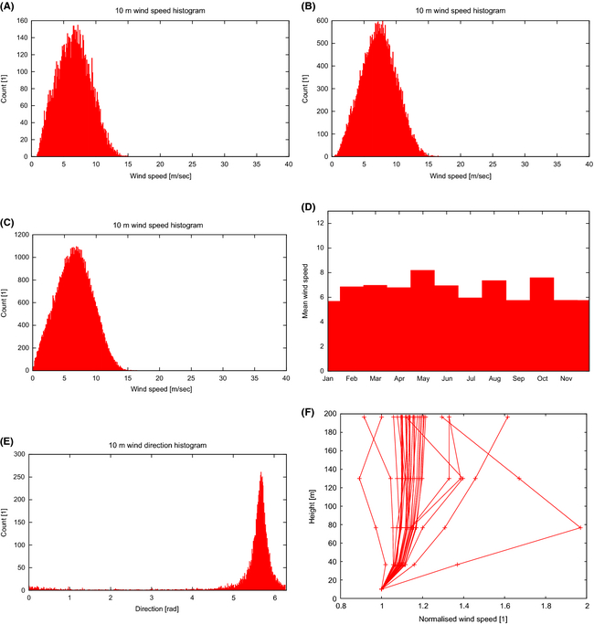
Here the winds are more reliable, with calmer events, rather than gustiness, Figure 18C, very similar to Baja California Sur. Exhibiting a very stable monthly seasonality, Figure 18D. The vertical profiles, Figure 18F, may suggest that height extrapolations have to be interpreted with caution.

Figure 18. North of Merida. (A) Daily mean wind speed. (B) 6 h max wind speed. (C) Three hour instantaneous wind speed. (D) Monthly mean. (E) Wind direction. (F) Vertical wind profile (normalized by 10 m wind speed).

Quintana Roo

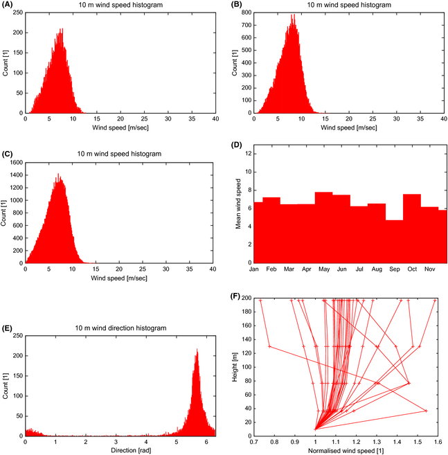
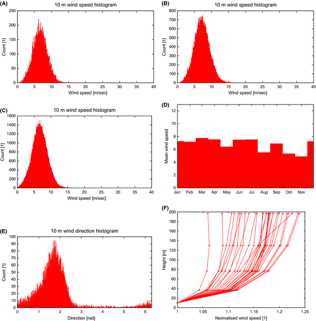
The results indicate a reliable source, certainly the vertical profiles are significantly more uniform, Figure 19F. A well-balanced histogram, Figure 19C, and stable low seasonal variation, more so in the first half of the year, Figure 19D, indicate that the 400–500 W/m² may be feasible here.

Figure 19. Quintara Roo. (A) Daily mean wind speed. (B) 6 h max wind speed. (C) Three hour instantaneous wind speed. (D) Monthly mean. (E) Wind direction. (F) Vertical wind profile (normalized by 10 m wind speed).

Comparison with other studies

There is also a good correspondence with the maps produced by NREL:

• In the Gulf of Tehuantepec, satellite data confirm the offshore potential above 1000 W/m² and also indicate a strong seasonal variability. There is very good agreement when compared to the satellite-derived WPD in [14]. Only a slight difference in location of the isolines (a couple of grid boxes), however this has to be expected when comparing climate data with an observational product. The seasonal dependence of the mean wind speed was reproduced here with an average high of around 10 m/sec in November–April and a low of around 6 m/sec in May to October (cf. Figure 16D).
• The local peak at the north western coast of Campeche, near Merida, as reported by NREL as “moderate/good” (200–250 W/m² at 30 m) [15] was also reproduced well here, with 200–300 W/m² at 10 m and 400–500 W/m² at 50 m, extending offshore. What can be seen on the NREL map as a thin sliver of “good” conditions along the east coast of Yucatan (250–350 W/m² at 30 m) can be seen to extend further into the Caribbean sea here with 200–300 W/m² at 10 m and 300–400 W/m² at 50 m.
• A hint toward “good to excellent” conditions (400–500 W/m² at 50 m) in the upper Gulf of California can be seen in the NREL map for western Sonora [16], where some coastal area is also covered. This is also reproduced here with 200–300 W/m² at 10 m and a more promising (and geographically more prominent) 300–400 W/m² at 50 m
• NREL reports localized “fair” conditions (300–400 W/m² at 50 m) along the west coast of Baja California and 200–250 W/m² at 30 m at isolated locations in Baja California Sur (without covering coastal or offshore locations) [17, 18]. Here, it can be seen that the conditions improve further offshore, with a sustained 300–400 W/m² at 50 m and even a peak toward 400–500 W/m². Although this peak is too small to be taken too serious, however it supports an estimate closer to 400 W/m² rather than 300 W/m² in that location.

Carrasco-Díaz et al. [19] summarize the Wind Power Potential for Tamaulipas coast as 200–300 W/m² for the southern coast and 400–500 W/m² in the northern half of the State. Here this has been reproduced, with the northern half also falling into the 400–500 W/m² at 50 m bracket. The estimate for the southern half is a slightly higher with 300–400 W/m² at 50 m, which seems reasonable as there would be no immediate explanation for the gap between the two estimates.

Conclusions and Further Work

The uncertainty involved in height extrapolation has been illustrated above. Also an improved methodology for extrapolation has been presented and the importance of moisture demonstrated. It is clear that the wind energy sector would benefit from additional diagnostics in climate model outputs and/or dedicated runs. Nevertheless, the current data can provide key guidance as to where to focus future investigation. Based on this work, dedicated downscaling experiments can now be performed, with specific setups, and with an increased number of vertical levels in the area of interest. This approach would eliminate the need for extrapolation.

Then, with the benefit of improved resolution, the results can be compared to predictions from coastal meteorological stations. In this study, the effect of orography and the land surface overall could not be taken into account satisfactorily and therefore has been deliberately excluded from the start. However, with the high-resolution results at hand, the error incurred by not having sufficient resolution in the present study can be quantified and the study area extended further inland with more confidence.

The high-resolution result, however, will also have to be treated with care: If there is one small area which is classed as very promising in an area otherwise termed uneconomic then there has to be a very good meteorological reason for this and not numerical error or variability. Too often are results presented at an incredible resolution and associated detail, however the confidence in such results has to be questioned thoroughly. The variability in the wind on the fine scale should in general quickly average out as long as the time series is long enough, removing this – in source temporal, in consequence spatial – pattern from the result. High values are expected along elevation, or where there are funneling effects due to the orography. But not randomly appearing without good reason (such as turbulence may manifest itself in a temporal snapshot).

Local observational data can now be sought just before deploying micrositing studies to further, incrementally, build confidence.

Acknowledgments

This work is based on the UPSCALE data set licensed from the University of Reading which includes material from NERC and the Controller of HMSO & Queens Printer. The UPSCALE data set was created by P. L. Vidale, M. Roberts, M. Mizielinski, J. Strachan, M. E. Demory and R. Schiemann using the HadGEM3 model with support from NERC and the Met Office and the PRACE Research Infrastructure resource HERMIT based in Germany at HLRS. The authors thank anonymous reviewer one for his time, dedication and thoroughness, providing plenty of recommendations which led to a significantly improved and clearer manuscript.

Conflict of Interest

None declared.

References

1. Carvalho, D., A. Rocha, C. Silva Santos, and R. Pereira. 2013. Wind resource modelling in complex terrain using different mesoscale-microscale coupling techniques. Appl. Energy108:493–504.
2. Ciesielski, P. E. and R. H. Johnson. 2008. Diurnal cycle of surface flows during 2004 NAME and comparison to model reanalysis. J. Clim.21:3890–3913.
3. Walters, D. N., M. J. Best, A. C. Bushell, D. Copsey, J. M. Edwards, P. D. Falloon, et al. 2011. The met office unified model global atmosphere 3.0/3.1 and JULES global land 3.0/3.1 configurations. Geosci. Model Dev.4:919–941. doi: 10.5194/gmd-4-919-2011.
4. Mizielinski, M. S., M. J. Roberts, P. L. Vidale, R. Schiemann, M. E. Demory, J. Strachan, et al. 2014. High-resolution global climate modelling: the upscale project, a large-simulation campaign. Geosci. Model Dev.7:1629–1640. doi: 10.5194/gmd-7-1629-2014.
5. Donlon, C. J., M. Martin, J. Stark, J. Roberts-Jones, E. Fiedler, and W. Wimmer. 2012. The operational sea surface temperature and sea ice analysis (ostia) system. Remote Sens. Environ.116:140–158. doi: 10.1016/j.rse.2010.10.017.
6. Sheffield, J., A. P. Barrett, B. Colle, D. N. Fernando, R. Fu, K. L. Geil, et al. 2013. North American climate in CMIP5 experiments. Part I: evaluation of historical simulations of continental and regional climatology. J. Climate26:92099245.
7. Sheffield, J., S. J. Camargo, R. Fu, Q. Hu, X. Jiang, N. Johnson, et al. 2013. North American climate in CMIP5 experiments. Part II: evaluation of historical simulations of intraseasonal to decadal variability. J. Climate26:92479290.
8. Kållberg, P., A. Simmons, S. Uppala, and M. Fuentes. 2004. The ERA-40 archive. Technical Report 17. ECMWF, Shinfield Park, Reading
9. Dee, D. P., S. M. Uppala, A. J. Simmons, P. Berrisford, P. Poli, S. Kobayashi, et al. 2011. The erainterim reanalysis: configuration and performance of the data assimilation system. QJR Meteorol. Soc.137:553–597. doi: 10.1002/qj.828.
10. Charney, J. G., and N. A. Phillips. 1953. Numerical integration of the quasi-geostrophic equations for barotropic and simple baroclinic flows. J. Meteorol.10:71–99.
11. Wood, N., A. Staniforth, A. White, T. Allen, M. Diamantakis, M. Gross, et al. 2014. An inherently mass-conserving semi-implicit semi-lagrangian discretization of the deep-atmosphere global non-hydrostatic equations. QJR Meteorol. Soc.140:1505–1520. doi: 10.1002/qj.2235.
12. Ahmed, S. 2011. Wind energy: theory and practice. PHI Learning, India.
13. Hsu, S. A., E. A. Meindl, and D. B. Gilhousen. 1994. Determining the power-law wind-profile exponent under near-neutral stability conditions at sea. J. Appl. Metrol.33:757–765.
14. Elliott, D., M. Schwartz, G. Scott, S. Haymes, D. Heimiller, and R. George. 2003. Wind energy resource atlas of Oaxaca. Technical Report. NREL, Colorado, USA.
15. NREL wind power density map for yucatan. Available at http://www.nrel.gov/wind/images/mexico-yucatan-windmap.gif (accessed 08 February 2015).
16. NREL wind power density map for western sonora. Available at http://www.nrel.gov/wind/pdfs/mexico_w_sonora.pdf. (accessed 08 February 2015).
17. NREL wind power density map for baja california. http://www.nrel.gov/wind/pdfs/mexico_baja.pdf. (accessed 08 February 2015).
18. NREL wind power density map for baja californiasur. http://www.nrel.gov/wind/pdfs/mexico-bajasur.pdf. (accessed 08 February 2015).
19. Carrasco-Díaz, M., D. Rivas, M. Orozco-Contreras, and O. Sánchez-Montante. 2015. An assessment of wind power potential along the coast of Tamaulipas, Northeastern México. Renewable Energy78:295–305. doi: 10.1016/j.renene.2015.01.007.