Explicit dynamic analysis of thin membrane structures

Abstract

An explicit dynamic structural solver developed at CIMNE for the analysis of parachutes is presented. The canopy fabric has a negligible out-of-plane stiffness, therefore its numerical study presents important challenges. Both the large changes in geometry and the statically indeterminate character of the system are problematic from the numerical point of view. This report covers the reasons behind the particular choice of solution scheme as well as a detailed description of the underlying algorithm. Both the theoretical foundations of the method and details of implementation aiming at improving computational efficiency are given. Benchmark cases to assess the accuracy of the solution as well as examples of practical application showing the performance of the code are finally presented.

1 Problem overview

This report describes the theoretical foundation as well as applications of PUMI_MEM, an explicit dynamics structural solver developed at CIMNE. This code is part of the PARAFLIGHT parachute simulation suite [1] which also includes a potential flow solver [2]. The mechanical analysis of thin membrane structures braced with cables (e.g. parachutes) is a challenging task. Two effects entail a host of numerical problems [3]:

• In general the structure is not statically determinate for an arbitrary set of loads (i.e. it behaves like a mechanism). Thus, it might be impossible to reach an equilibrium state without drastic changes in geometry. The structural response is therefore highly nonlinear and may cause severe convergence problems.

• Due to the virtually zero bending stiffness of the components the material behaviour is irreversible. The fabric is able to resist tensile stresses but buckles (wrinkles) almost immediately under compressive loads. This asymmetric behaviour further complicates the mechanical analysis [4][5].

In the particular case of parachutes there is an additional complication due to the nature of the applied forces. These being mostly pressure loads, their direction is not known a priori but is a function of the deformed shape and must therefore be computed as part of the solution. This is an additional source of non-linearity. Finally, matters are further complicated by the extreme sensitivity of the pressure field to changes in geometry [6].

In view of these challenges it was decided to use a finite element (FE) dynamic structural solver. An unsteady analysis is insensitive to the problems caused by the lack of a definite static equilibrium configuration. In a dynamic problem the structure is constantly in equilibrium with the inertial forces so the solution is always unique. Even if only the long-term static response is sought the dynamic study offers clear advantages. Furthermore, the extension to transient dynamic problems becomes trivial. There are two basic kinds of dynamic solvers, implicit and explicit [7]. Their main features are:

• Implicit: Can be made unconditionally stable (allows for large time steps). Cost per time step is large, each step requires solving a non linear problem using an iterative algorithm. The radius of convergence of the iterative algorithms is however limited so the time step cannot be made arbitrarily large.

• Explicit: Only conditionally stable. The stability limit is determined by the material properties and the geometry of the FE mesh. Cost per time step is low.

When the structural response does not deviate much from linearity the implicit treatment is advantageous as it allows advancing in time quickly. Also, the static equilibrium (when it exists) can be reached in a small number of iterations. However, when the behaviour is heavily non-linear, the time increment must be cut back in order for the iterative schemes to converge and the computational increases quickly. There is also a loss of robustness caused by the possibility of the algorithms failing to converge. On the other hand, the explicit method is extremely insensitive to these effects and requires a number of time steps that does not change substantially as the system response becomes more complex. Material non-linearities and large displacements which are extremely detrimental for the convergence behaviour of the implicit scheme do not affect so adversely the explicit algorithm.

In view of the difficulties expected the choice was made to use an Explicit FE structural solver. A further advantage is the ability of the algorithm to be easily vectored and thus take advantage of modern parallel processing architectures. Linear cable and membrane elements where selected due to their ease of implementation. The fabric is modelled using three-node membrane elements due to their geometric simplicity. As the three nodes of the element can be always assumed to lie in a plane, the definition of the local coordinate systems is straightforward. When a quadrilateral element is passed from the aerodynamic solver, it is internally transformed into a pair of triangular elements in order to carry the analysis.

A local corrotational reference frame is used for each cable and membrane element in order to remove the large rigid-body displacement field and isolate the material strains. Inside each element a simple small-strain formulation is used due to the properties of the fabric. Tensile deformations are always small, on the other hand compressive strains can become extremely large due to the inclusion of a wrinkling model (zero compression stiffness). There is however no stress associated with the compressive strains and, correspondingly, no strain energy. The small-strain formulation is therefore adequate, as only the small tensile deformations must be into account to calculate the stress state.

While not strictly necessary to model the parachute behaviour, tetrahedral solid (3D) elements have been included in the code. They prove useful in modelling the dynamic interaction between the parachute and its payload. As they are meant to model bodies undergoing only small deformations a linear formulation is considered adequate for the task at hand.

2 Problem Formulation

2.1 Weak equilibrium statement

We start using the internal equilibrium statement for a continuum which relates the gradient of the stress field to the applied loads

${\begin{array}{c}\sum _{j}{\frac {\partial {\sigma }_{ij}}{\partial x_{j}}}+b_{i}=0{\mbox{ }}{\mbox{ }}{\mbox{ }}{\mbox{ }}{\mbox{ }}\forall {\mbox{ }}{\mbox{ }}{\mbox{ }}{\boldsymbol {x}}\in \Omega {\mbox{ }}{\mbox{ }}{\mbox{ }}{\mbox{ }}{\mbox{ }}i=1,2,3\\u_{i}={\overline {u}}_{i}({\boldsymbol {x}}){\mbox{ }}{\mbox{ }}{\mbox{ }}{\mbox{ }}{\mbox{ }}\forall {\mbox{ }}{\mbox{ }}{\mbox{ }}{\boldsymbol {x}}\in {\Gamma }_{D}\\\sum _{j}{\sigma }_{ij}\cdot n_{j}={\overline {t}}_{i}({\boldsymbol {x}}){\mbox{ }}{\mbox{ }}{\mbox{ }}{\mbox{ }}{\mbox{ }}\forall {\mbox{ }}{\mbox{ }}{\mbox{ }}{\boldsymbol {x}}\in {\Gamma }_{N}{\mbox{ }}{\mbox{ }}{\mbox{ }}{\mbox{ }}\end{array}}$

(2.1)

were ${\textstyle {\overline {u}}_{i}}$ and ${\textstyle {\overline {t}}_{i}}$ stand for prescribed surface displacements and tractions. In the case of a dynamic problem the body forces (b_i) include the inertial loads given by:

${b_{i}\vert }_{inertial}=-\rho {\frac {d^{2}u_{i}}{dt^{2}}}$

(2.2)

where ρ is the density of the solid. Note that the time derivative in (2.2) is a total one, i.e. tracking the material particles. To obtain the Finite Element (FE) formulation of the problem we construct the weak formulation of (2.1). Let δu_i be an arbitrary test function (representing in this case a virtual displacement field). We may thus write:

${\begin{array}{c}\left({\frac {\partial {\sigma }_{ij}}{\partial x_{j}}}+b_{i}\right)\delta u_{i}=0{\mbox{ }}{\mbox{ }}{\mbox{ }}{\mbox{ }}{\mbox{ }}\forall {\mbox{ }}{\mbox{ }}{\mbox{ }}{\boldsymbol {x}}\in \Omega {\mbox{ }}{\mbox{ }}{\mbox{ }}{\mbox{ }}{\mbox{ }}i=1,2,3\\\left(u_{i}-{\overline {u}}_{i}\right)\delta u_{i}=0{\mbox{ }}{\mbox{ }}{\mbox{ }}{\mbox{ }}{\mbox{ }}\forall {\mbox{ }}{\mbox{ }}{\mbox{ }}{\boldsymbol {x}}\in {\Gamma }_{D}\\\left({\sigma }_{ij}\cdot n_{j}-{\overline {t}}_{i}\right)\delta u_{i}=0{\mbox{ }}{\mbox{ }}{\mbox{ }}{\mbox{ }}{\mbox{ }}\forall {\mbox{ }}{\mbox{ }}{\mbox{ }}{\boldsymbol {x}}\in {\Gamma }_{N}\end{array}}$

(2.3)

Note that in (2.3) implicit summation has been used in order to keep the notation compact. Now, the weighted average of the equations is taken over the relevant domains

$\int _{\Omega }\left({\frac {\partial {\sigma }_{ij}}{\partial x_{j}}}\delta u_{i}+\right.$$\left.b_{i}\delta u_{i}\right)d\Omega +\int _{{\Gamma }_{D}}\left(u_{i}\delta u_{i}-\right.$$\left.{\overline {u}}_{i}\delta u_{i}\right)d\Gamma +\int _{{\Gamma }_{N}}\left({\overline {t}}_{i}\delta u_{i}-\right.$$\left.{\sigma }_{ij}\cdot n_{j}\delta u_{i}\right)d\Gamma =$$0$

(2.4)

If (2.4) holds for any virtual displacement field, the equation becomes equivalent to (2.5). To keep the expressions simple without loss of generality it is common practice to assume that the virtual displacement field is compatible with any existing prescribed displacement constraints. This way the integrals over Γ_D can be dropped (i.e. $\delta u_{i}=0{\mbox{ }}{\mbox{ }}\forall {\mbox{ }}{\mbox{ }}{\boldsymbol {x}}\in {\Gamma }_{D}$ ) but care must be taken to ensure that the solution is indeed compatible with the constraints. The term containing the internal stresses can be integrated by parts yielding

$\int _{\Omega }\left(-{\sigma }_{ij}{\frac {\partial \delta u_{i}}{\partial x_{j}}}+\right.$$\left.b_{i}\delta u_{i}\right)d\Omega +\int _{{\Gamma }_{N}}{\overline {t}}_{i}\delta u_{i}{\mbox{ }}d\Gamma =$$0$

(2.6)

The deformation gradient can be split into a symmetric and an antisymmetric part:

${\frac {\partial \delta u_{i}}{\partial x_{j}}}={\frac {1}{2}}\left({\frac {\partial \delta u_{i}}{\partial x_{j}}}+\right.$$\left.{\frac {\partial \delta u_{j}}{\partial x_{i}}}\right)+$${\frac {1}{2}}\left({\frac {\partial \delta u_{i}}{\partial x_{j}}}-\right.$$\left.{\frac {\partial \delta u_{j}}{\partial x_{i}}}\right)=$$\delta {\epsilon }_{ij}+\delta {\omega }_{ij}$

(2.7)

In the expression above ε_ij represents the virtual strain field and ω_ij is the virtual local rotation. Given that the stress tensor is symmetric the product ${\sigma }_{ij}{\omega }_{ij}$ vanishes. Expression (2.6) then becomes the virtual work principle

$\sum _{i,j}\int _{\Omega }{\sigma }_{ij}\delta {\epsilon }_{ij}{\mbox{ }}d\Omega =$$\sum _{i}\int _{\Omega }b_{i}\delta u_{i}{\mbox{ }}d\Omega +$$\sum _{i}\int _{{\Gamma }_{N}}{\overline {t}}_{i}\delta u_{i}{\mbox{ }}d\Gamma$

(2.8)

Eq. (2.8) states that when the system is in equilibrium the change in strain energy caused by an arbitrary virtual displacement field equals the work done by the external forces.

2.2 Finite element discretization

To obtain the FE discretization we build an approximate solution interpolating the nodal values of the displacements [8]. A virtual displacement field can be obtained in the same way

${\tilde {u}}_{i}({\boldsymbol {x}})=N^{k}({\boldsymbol {x}}){\mbox{ }}{\tilde {u}}_{i}^{k}{\mbox{ }}{\mbox{ }}{\mbox{ }}{\mbox{ }}{\mbox{ }}{\mbox{ }}{\mbox{ }}\delta u_{i}({\boldsymbol {x}})=$$N^{l}({\boldsymbol {x}}){\mbox{ }}\delta u_{i}^{l}$

(2.9)

In (2.9) ${\textstyle {\tilde {u}}}$ represents the approximate solution and N^k is the interpolation function corresponding to the k^th node (called a shape function). From now on supra-indexes will be used to indicate nodal values. The virtual strain field is a linear function of the virtual displacement field so it also a linear function of ${\textstyle \delta u_{i}^{l}}$ , it is possible therefore to write

$\delta {\epsilon }_{ij}=A_{ij,m}^{l}\delta u_{m}^{l}{\mbox{ }}{\mbox{ }}{\mbox{ }}{\mbox{ }}{\mbox{ }}{\mbox{ }}{\mbox{ }}{\mbox{ }}A_{ij,m}^{l}=$${\frac {\partial {\epsilon }_{ij}}{\partial u_{m}^{l}}}=L(N^{l})$

(2.10)

With the $A_{ij,k}^{l}$ coefficients being linear functions of the shape function gradients. For a dynamic problem the inertial term (2.2) is discretized as

${{\tilde {b}}_{i}\vert }_{inertial}=-\rho N^{k}{\frac {d^{2}u_{i}^{k}}{dt^{2}}}$

(2.11)

As the shape functions are not functions of time (their value does not change for a given material point) the time derivative in (2.11) affects only the nodal displacements. Rearranging equation (2.8) so only the inertial term remains on the LHS yields

$\int _{\Omega }\rho N^{k}{\frac {d^{2}u_{i}^{k}}{dt^{2}}}N^{l}\delta u_{i}^{l}{\mbox{ }}d\Omega =$$\int _{\Omega }b_{i}N^{l}\delta u_{i}^{l}{\mbox{ }}d\Omega +$$\int _{{\Gamma }_{N}}{\overline {t}}_{i}N^{l}\delta u_{i}^{l}{\mbox{ }}d\Gamma -$$\int _{\Omega }{\sigma }_{ij}A_{ij,m}^{l}\delta u_{m}^{l}{\mbox{ }}d\Omega$

(2.12)

As the virtual nodal displacements are arbitrary, it is possible to set all but one of them to zero. This way as many equations as degrees of freedom existing on the system are obtained. By setting

${\textstyle \delta u_{a}^{b}=1{\mbox{ }}{\mbox{ }}{\mbox{ }}{\mbox{ }}{\mbox{ }}{\mbox{ }};{\mbox{ }}{\mbox{ }}{\mbox{ }}{\mbox{ }}{\mbox{ }}{\mbox{ }}\delta u_{a}^{b}=}$$1{\mbox{ }}{\mbox{ }}:{\mbox{ }}{\mbox{ }}i\not =a{\mbox{ }}{\mbox{ }},{\mbox{ }}{\mbox{ }}j\not =$$b$

(2.13)

The following set of equations is obtained:

$\int _{\Omega }\rho N^{b}N^{k}d\Omega {\frac {d^{2}u_{a}^{k}}{dt^{2}}}=$$\int _{\Omega }b_{a}N^{b}d\Omega +\int _{{\Gamma }_{N}}{\overline {t}}_{a}N^{b}d\Gamma -$$\int _{\Omega }{\sigma }_{kj}A_{kj,a}^{b}d\Omega {\mbox{ }}{\mbox{ }}{\mbox{ }}{\mbox{ }}{\mbox{ }}\lbrace {\begin{array}{c}a=1,2,3\\b=1,...,n_{nod}\end{array}}$

(2.14)

In the equation above sum is assumed over j & k. The equations can also be written in matrix form as

${\boldsymbol {M{\ddot {u}}}}={\boldsymbol {b}}+{\boldsymbol {t}}-$${\boldsymbol {I}}$

(2.15)

M is called the mass matrix, b and t are the external nodal generalized forces and I is the internal force vector. If the mechanical response is linear the stress tensor can be written as a linear combination of the nodal displacements. The internal force vector can then be recast as

${\boldsymbol {I=Ku}}$

(2.16)

where K is the stiffness matrix of the system. Even if the behaviour of the structure is not truly linear, this may be useful as a linearization around some base state.

It is possible to solve for the acceleration in (2.15) by inverting the mass matrix

${\boldsymbol {\ddot {u}}}={\boldsymbol {M}}^{\boldsymbol {-1}}\left[{\boldsymbol {b}}+\right.$$\left.{\boldsymbol {t}}-{\boldsymbol {I}}\right]$

(2.17)

The system of ODEs (2.17) together with the suitable initial conditions

${\begin{array}{c}{{\boldsymbol {u}}\vert }_{t=o}={\boldsymbol {u}}_{\boldsymbol {0}}\\{{\boldsymbol {\dot {u}}}\vert }_{t=o}={\boldsymbol {\dot {u}}}_{\boldsymbol {0}}\end{array}}$

(2.18)

can be advanced in time to yield the displacement field at every instant. Solving for the acceleration term in (2.17) requires inverting the mass matrix. To speed up the computations without significant loss of accuracy, the mass matrix is usually replaced by its lumped (diagonal) counterpart

$M_{ij}^{d}={\delta }_{ij}\sum _{j}M_{ij}$

(2.19)

In the expression above ${\textstyle {\delta }_{ij}}$ represents the Kronecker delta function (i.e. one when i=j and zero otherwise).

In order to form the matrix and load vectors appearing in (2.15) an element-by-element approach is used. As the shape function of node k is nonzero only inside elements containing said node, the integrals need only evaluated in the appropriate elements, for example:

$M_{ij}=\int _{\Omega }\rho N^{i}N^{j}d\Omega =\sum _{el}\int _{{\Omega }_{el}}\rho N^{i}N^{j}d\Omega {\mbox{ }}{\mbox{ }}{\mbox{ }}{\mbox{ }}{\mbox{ }}{\mbox{ }}/{\mbox{ }}{\mbox{ }}{\mbox{ }}i,j\subset el$

(2.20)

2.3 Time integration

The integration of the system (2.17) can be performed using both implicit and explicit schemes [7]. For the reasons outlined previously, the explicit method has been chosen. The explicit second order central differencing scheme has been selected due to its high efficiency coupled with acceptable accuracy. Given a series of points in time and their corresponding time increments

${\begin{array}{c}t^{\left(0\right)}{\mbox{ }}{\mbox{ }}{\mbox{ }},{\mbox{ }}{\mbox{ }}{\mbox{ }}...{\mbox{ }}{\mbox{ }}{\mbox{ }},{\mbox{ }}{\mbox{ }}{\mbox{ }}t^{\left(i-1\right)}{\mbox{ }}{\mbox{ }}{\mbox{ }},{\mbox{ }}{\mbox{ }}{\mbox{ }}t^{\left(i\right)}{\mbox{ }}{\mbox{ }}{\mbox{ }},{\mbox{ }}{\mbox{ }}{\mbox{ }}t^{\left(i+1\right)}{\mbox{ }}{\mbox{ }}{\mbox{ }},{\mbox{ }}{\mbox{ }}{\mbox{ }}...\\...{\mbox{ }}{\mbox{ }}{\mbox{ }},{\mbox{ }}{\mbox{ }}{\mbox{ }}\Delta t^{\left(i\right)}=t^{\left(i\right)}-t^{\left(i-1\right)}{\mbox{ }}{\mbox{ }}{\mbox{ }},{\mbox{ }}{\mbox{ }}{\mbox{ }}\Delta t^{\left(i+1\right)}=t^{\left(i+1\right)}-t^{\left(i\right)}{\mbox{ }}{\mbox{ }}{\mbox{ }},{\mbox{ }}{\mbox{ }}{\mbox{ }}...\end{array}}$

(2.21)

let us define the change in midpoint velocity as

${\frac {d{\boldsymbol {u}}}{dt}}^{\left(i+{\frac {1}{2}}\right)}-$${\frac {d{\boldsymbol {u}}}{dt}}^{\left(i-{\frac {1}{2}}\right)}=$${\frac {\Delta t^{\left(i+1\right)}+\Delta t^{\left(i\right)}}{2}}\cdot {\frac {d^{2}{\boldsymbol {u}}^{\left(i\right)}}{dt^{2}}}$

(2.22)

Observe that in (2.22) the accelerations and velocities are expressed at different instants. This scheme provides second order time-accuracy by virtue of using a centered approximation for the time derivative. Once the intermediate velocities have been computed, the displacements can be updated

${\boldsymbol {u}}^{\left(i+1\right)}={\boldsymbol {u}}^{\left(i\right)}+$$\Delta t^{\left(i+1\right)}\cdot {\frac {d{\boldsymbol {u}}^{\left(i+{\frac {1}{2}}\right)}}{dt}}=$${\boldsymbol {u}}^{\left(i\right)}+\Delta t^{\left(i+1\right)}\cdot \left[{\frac {d{\boldsymbol {u}}}{dt}}^{\left(i-{\frac {1}{2}}\right)}+\right.$$\left.{\frac {\Delta t^{\left(i+1\right)}+\Delta t^{\left(i\right)}}{2}}\cdot {\frac {d^{2}{\boldsymbol {u}}^{\left(i\right)}}{dt^{2}}}\right]$

(2.23)

This scheme is fully explicit in that sense that if ${\boldsymbol {u}}^{\left(i\right)}{\mbox{ }},{\mbox{ }}{\frac {d{\boldsymbol {u}}}{dt}}^{\left(i-{\frac {1}{2}}\right)}{\mbox{ }},{\mbox{ }}{\frac {d^{2}{\boldsymbol {u}}^{\left(i\right)}}{dt^{2}}}$ are kwon, it is possible to compute the updated displacement and velocity without the need to solve any equations. That is, (2.23) yields the new values without the need to solve any additional equation. Obviously the method is not self-starting, as at the initial time step the value of ${\frac {d{\boldsymbol {u}}}{dt}}^{\left(-{\frac {1}{2}}\right)}$ is not known (the initial conditions (2.18) are specified for i=0). To deal with this inconvenience we may use one sided differencing to estimate the velocity at i=+1/2

${\frac {d{\boldsymbol {u}}}{dt}}^{\left(+{\frac {1}{2}}\right)}=$${\frac {d{\boldsymbol {u}}}{dt}}^{\left(0\right)}+{\frac {\Delta t^{\left(1\right)}}{2}}\cdot {\frac {d^{2}{\boldsymbol {u}}^{\left(0\right)}}{dt^{2}}}$

(2.24)

Using this value together with (2.22) gives

${\frac {d{\boldsymbol {u}}}{dt}}^{\left(-{\mbox{ }}{\frac {1}{2}}\right)}=$${\frac {d{\boldsymbol {u}}}{dt}}^{\left(0\right)}-{\frac {\Delta t^{\left(0\right)}}{2}}\cdot {\frac {d^{2}{\boldsymbol {u}}^{\left(0\right)}}{dt^{2}}}$

(2.25)

Using this dummy velocity value the time integration can be started. Please remark that the choice of $\Delta t^{\left(0\right)}$ has no effect on the final result. The method outlined has an extremely low computational cost per time step, however it shows a very important limitation. The explicit scheme is only conditionally stable meaning the time step cannot be made arbitrarily large lest the solution diverges. The maximum allowable time step is given by

$\Delta t\leq {\frac {2}{{\omega }_{max}}}$

(2.26)

with ω_max being the angular frequency of the highest eigenmode of the system. The expression (2.26) is truly valid only for undamped systems. If damping is included in the model (it always is for practical reasons) then its effect can be accounted for trough

$\Delta t\leq {\frac {2}{{\omega }_{max}}}\cdot \left({\sqrt {1+{\xi }^{2}}}-\right.$$\left.\xi \right)$

(2.27)

In the expression above ξ is the damping ratio of the highest eigenmode. From (2.27) it becomes obvious that damping can have a very detrimental effect on the stability limit. While (2.27) provides a very good estimate of the allowable time step, it is not practical to calculate the highest eigenvalue of the system as this calls for solving a complex problem (the number of degrees of freedom in the model can be very large). Fortunately there is a simple upper bound estimate of ω_max

${\omega }_{max}\leq {\omega }_{max}^{elem}$

(2.28)

with ${\omega }_{max}^{elem}$ being the highest elemental eigenfrequency in the model. The interaction with neightbouring elements always causes the highest system eigenmode to be slower than the highest isolated-element normal mode. Thus a conservative stability limit can be used in place of (2.26)

$\Delta t\leq {\frac {2}{{\omega }_{max}^{elem}}}$

(2.29)

The maximum frequency is associated with dilatational modes. An alternative estimate of the maximum time step is given by the minimum transit time of the dilatational waves across the elements of the mesh:

$\Delta t\leq min\left({\frac {L_{e}}{c_{d}}}\right)$

(2.30)

In (2.30) L_e is some characteristic element dimension and c_d is the dilatational wave speed. For an isotropic linear elastic solid

${\begin{array}{c}c_{d}={\sqrt {\frac {\lambda +2\mu }{\rho }}}\\\lambda =K-{\frac {2}{3}}G{\mbox{ }}{\mbox{ }}{\mbox{ }}{\mbox{ }}{\mbox{ }};{\mbox{ }}{\mbox{ }}{\mbox{ }}{\mbox{ }}\mu =G={\frac {E}{2(1+\nu )}}{\mbox{ }}{\mbox{ }}{\mbox{ }}{\mbox{ }}{\mbox{ }};{\mbox{ }}{\mbox{ }}{\mbox{ }}{\mbox{ }}K={\frac {E}{3\left(1-2\nu \right)}}\end{array}}$

(2.31)

where λ and μ are the Lamé constants which can be calculated from the shear modulus (G) and bulk modulus (K) as stated above.

2.4 Mass scaling

If a poor quality mesh is used, some degenerate elements (i.e. having close to zero volume) might be present. These can be extremely detrimental to the performance of the algorithm as their associated characteristic lengths will be very small. Hence, the global stability limit given by (2.30) becomes extremely low, calling for a large number of time steps in order to finish the simulation. To overcome this problem the code includes a selective mass scaling options which introduces local changes in the element density in order to keep the stability limit within acceptable levels. For those elements where the value given by (2.30) is considered excessively small the density is artificially augmented in order to decrease the wave speed (2.31). The user can select the maximum acceptable scatter in the elemental stability limits and the code (using the statistics for the complete model) automatically corrects the elements falling outside the established bounds. It must be stressed that the effect of the increased density on the global dynamic response is very small because the elements affected are only those with very small volumes. As the mass of these elements, even after scaling, is a negligible fraction of the total system mass the overall behaviour of the structure is almost unchanged (i.e. the inertial properties remain basically the same). In those cases where only the system’s static response in sought, mass scaling can be used in a more aggressive manner without altering the solution.

3 Numerical damping

To achieve a smooth solution it is always needed to introduce some amount of damping into the numerical model. In a real structure different types of damping are always present (e.g. material, aerodynamic, etc…) so the observed behaviour is usually smooth. On the other hand, the dissipation provided by the basic explicit algorithm is really small. This is a problem when a steady state solution is sought but is also undesirable when simulating transient events as high frequency noise can contaminate the solution. To allow greater flexibility controlling the solution process two forms of user-adjustable damping are provided; Rayleigh damping and bulk viscosity. In the first case a damping matrix is built from the mass and stiffness matrices:

${\boldsymbol {C}}=\alpha {\boldsymbol {M}}+\beta {\boldsymbol {K}}$

(3.1)

The equation system (2.15) supplemented with this damping term becoming

${\boldsymbol {M{\ddot {u}}}}={\boldsymbol {b}}+{\boldsymbol {t}}-$${\boldsymbol {I}}-{\boldsymbol {C{\dot {u}}}}$

(3.2)

The α term creates a damping force which is proportional to the absolute velocity of the nodes. This is roughly equivalent to having the nodes of the structure move trough a viscous fluid. The damping ratio introduced by the mass proportional damping term on a mode of frequency ω is

$\xi ={\frac {\alpha }{2\omega }}$

(3.3)

From (3.3) it is apparent that the α term affects mainly the low frequency components of the solution. It can be useful to accelerate convergence to a static solution when only the long-term response is sought. However, when the transient response must be accurately determined this factor should not be included (or at least the α parameter must be chosen in order to ensure the damping ratio for the lowest mode is very small). The β term on the other hand introduces forces that are proportional to the material strain rate. An extra stress σ_d is added to the constitutive law

${\boldsymbol {\sigma }}_{\boldsymbol {d}}=\beta {\boldsymbol {D}}^{\boldsymbol {el}}{\boldsymbol {:{\dot {\epsilon }}}}$

(3.4)

with D^el being the tangent stiffness tensor of the material. The fraction of critical damping for a given mode is:

$\xi ={\frac {\beta {\mbox{ }}\omega }{2}}$

(3.5)

In this case only the high order modes are affected appreciably. This is desirable as it prevents high frequency noise from propagating while leaving the low order response (which is usually the part sought) almost unchanged. The β parameter however must be used sparingly, as it has a very detrimental effect on the stability limit (because its effect is greatest for the highest eigenmode of the system).

An additional form of damping is included to prevent high frequency “ringing”. This is caused by excitation of element dilatational modes which are always associated with the highest eigenvalues of the system. An additional hydrostatic stress is included in the constitutive routines which is proportional to the volumetric strain rate. This volumetric viscous stress is given by

${\sigma }_{h}=b_{1}{\mbox{ }}\rho {\mbox{ }}c_{d}{\mbox{ }}L_{e}{\mbox{ }}{\dot {\epsilon }}_{vol}$

(3.6)

In the expression above b₁ is the desired damping ratio for the dilatational mode. A suitable value is b₁=0,06.

4 Element formulation

The elements chosen are linear two-node cables and three node membranes. As an introduction to the details of implementation the cable element formulation is described first. While extremely simple, it contains many of the relevant features needed to formulate the surface element. As only small tensile strains are expected, a small-strain formulation has been adopted to calculate the elemental stresses. This assumption allows for efficient coding while maintaining acceptable accuracy.

4.1 Two-node linear cable element

Let us consider a linear element stretching between nodes i and j

Fig. 1 – Linear cable element internal and external loads

An external distributed loading per unit length ${\textstyle {\boldsymbol {f}}_{\boldsymbol {d}}}$ acts on the element whose cross sectional area will be denoted by A. As we shall be facing a large displacement problem, the position of the nodes can be written either on the undeformed (reference) configuration or in the deformed (current) configuration. From now on we shall use upper-case letters to denote the original coordinates while lower-case will be reserved for the current configuration. For example, the original length of the cable element is given by

$L_{0}=\Vert {\boldsymbol {X}}_{\boldsymbol {j}}-{\boldsymbol {X}}_{i}\Vert$

(4.1)

while the actual length at any given time is

$L(t)=\Vert {\boldsymbol {x}}_{\boldsymbol {j}}-{\boldsymbol {x}}_{\boldsymbol {i}}\Vert$

(4.2)

The unit vector along the element is

${\boldsymbol {e}}_{\boldsymbol {l}}={\frac {{\boldsymbol {x}}_{\boldsymbol {j}}-{\boldsymbol {x}}_{\boldsymbol {i}}}{\Vert {\boldsymbol {x}}_{\boldsymbol {j}}-{\boldsymbol {x}}_{\boldsymbol {i}}\Vert }}$

(4.3)

From the change in length of the element the axial strain and stress can be obtained. Assuming linear elastic behaviour:

$\epsilon ={\frac {L-L_{0}}{L_{0}}}{\mbox{ }}{\mbox{ }}{\mbox{ }}{\mbox{ }};{\mbox{ }}{\mbox{ }}{\mbox{ }}{\mbox{ }}\sigma =$$max(0{\mbox{ }},{\mbox{ }}E\epsilon )$

(4.4)

As we assume the cables buckle instantly under compressive loads, there is a lower bound on the allowable stresses. Therefore in (4.4) a minimum stress value of zero is enforced. Using this result the internal forces at the nodes become:

${\boldsymbol {I}}_{\boldsymbol {i}}=-\sigma A{\boldsymbol {e}}_{\boldsymbol {l}}{\mbox{ }}{\mbox{ }}{\mbox{ }}{\mbox{ }};{\mbox{ }}{\mbox{ }}{\mbox{ }}{\mbox{ }}{\boldsymbol {I}}_{\boldsymbol {j}}=$$+\sigma A{\boldsymbol {e}}_{\boldsymbol {l}}$

(4.5)

The nodal generalized external force due to the distributed loading is calculated as indicated in (2.14). If the load ${\textstyle {\boldsymbol {f}}_{\boldsymbol {d}}}$ is constant across the element it reduces to:

${\boldsymbol {b}}_{\boldsymbol {i}}=\int _{0}^{L}N_{i}{\boldsymbol {f}}_{\boldsymbol {d}}dL=$${\frac {L}{2}}{\boldsymbol {f}}_{\boldsymbol {d}}$

(4.6)

When numerical damping is included the stress term in (4.4) is augmented with the viscous contributions

${\frac {d\epsilon }{dt}}={\frac {({\boldsymbol {\dot {x}}}_{\boldsymbol {j}}-{\boldsymbol {\dot {x}}}_{\boldsymbol {i}})\cdot {\boldsymbol {e}}_{\boldsymbol {1}}}{L_{0}}}{\mbox{ }}{\mbox{ }}{\mbox{ }}{\mbox{ }};{\mbox{ }}{\mbox{ }}{\mbox{ }}{\mbox{ }}\sigma =$$E\left(max(0{\mbox{ }},{\mbox{ }}\epsilon )+\beta {\dot {\epsilon }}\right)+$$b{\mbox{ }}\rho {\mbox{ }}c_{d}{\mbox{ }}L_{0}{\mbox{ }}{\dot {\epsilon }}$

(4.7)

Note that in (4.7) the bulk viscosity term is slightly modified as it includes the axial strain rate instead of the volumetric strain rate. While using equations (4.1)-(4.7) is the most efficient way to calculate the internal forces for the element in a large displacement problem, it is also useful to have a closed expression for the elemental stiffness matrix (if the Rayleigh damping matrix is needed for example). This is specially simple if a local reference frame aligned with the element is chosen:

Fig. 2 – Cable local reference frame

For a virtual displacement of the end nodes we can calculate the change in length and in stress as

$\delta L=\delta u_{\zeta }^{j}-\delta u_{\zeta }^{j}{\mbox{ }}{\mbox{ }}{\mbox{ }}\Rightarrow {\mbox{ }}{\mbox{ }}{\mbox{ }}\delta \sigma =$${\frac {E}{L_{0}}}\left(\delta u_{\zeta }^{j}-\delta u_{\zeta }^{j}\right)$

(4.8)

Thus, the element stiffness matrix in the local coordinate system is given by

${\boldsymbol {K}}={\frac {EA}{L_{0}}}\left[{\begin{array}{cc}1&-1\\-1&1\end{array}}\right]$

(4.9)

Of course, the stiffness matrix is taken as zero whenever compressive strains exist in the element. The mass matrix can be obtained using (2.20) and the expressions of the shape functions in the local reference frame

${\begin{array}{c}N^{i}=1-{\frac {\xi }{L}}{\mbox{ }}{\mbox{ }}{\mbox{ }}{\mbox{ }};{\mbox{ }}{\mbox{ }}{\mbox{ }}{\mbox{ }}N^{j}={\frac {\xi }{L}}\\{\boldsymbol {M}}=\rho AL\left[{\begin{array}{cc}{\frac {1}{3}}&{\frac {1}{6}}\\{\frac {1}{6}}&{\frac {1}{3}}\end{array}}\right]\end{array}}$

(4.10)

As previously stated, the diagonal form of the mass matrix is usually preferred, thus (4.10) is replaced with:

${\boldsymbol {M}}^{\boldsymbol {d}}={\frac {\rho AL}{2}}\left[{\begin{array}{cc}1&0\\0&1\end{array}}\right]$

(4.11)

The element characteristic size used to estimate the allowable time step (2.30) for the case of a simple cable element is taken as L₀ (the cable reference length). Note that it is not necessary to consider the possibility of smaller values as a cable under compression shows no stiffness and therefore has a vanishing elastic wave speed. Due to the one-dimensional character of the problem, the dilatational wave speed can be safely replaced with the longitudinal wave speed

$c_{l}={\sqrt {\frac {E}{\rho }}}$

(4.12)

4.2 Three-node linear membrane element

Given that large displacements are expected, the strain state of the element is easier to assess using a local corrotational frame than in the global reference system [9]. Let us consider a triangular element defined by its three corner nodes

Fig. 3 – Triangle local reference frame

The three unit vectors along the local axes are obtained from

${\boldsymbol {e}}_{\boldsymbol {1}}={\frac {{\boldsymbol {x}}^{2}{-}{\boldsymbol {x}}^{1}}{\Vert {\boldsymbol {x}}^{2}{-}{\boldsymbol {x}}^{1}\Vert }}~;~{\boldsymbol {n}}={\frac {{\boldsymbol {e}}_{1}\times ({\boldsymbol {x}}^{3}{-}{\boldsymbol {x}}^{1})}{\Vert {\boldsymbol {e}}_{1}\times ({\boldsymbol {x}}^{3}{-}{\boldsymbol {x}}^{1})\Vert }}{\mbox{ }};{\mbox{ }}{\boldsymbol {e}}_{2}={\boldsymbol {n}}\times {\boldsymbol {e}}_{1}$

(4.13)

Any point of the triangle can now be identified by its two local coordinates (ξ,η)

$(\xi ,\eta )=\left(({\boldsymbol {x-}}{\boldsymbol {x}}^{1})\cdot {\boldsymbol {e}}_{1},({\boldsymbol {x}}-{\boldsymbol {x}}^{1})\cdot {\boldsymbol {e}}_{2}\right)$

(4.14)

As a linear triangle always remains flat, the problem is greatly simplified by analysing the stress state on the ξ-η plane.

Fig. 4 – Nodal coordinates in the local triangle reference frame

It is worth mentioning that the strain state of the triangle depends only on three parameters, as some of the nodal coordinates vanish in the corrotational reference frame (Fig. 4). In Fig. 4 the original (undeformed) geometry has been denoted with the subindex 0. The material strain is obtained from the interpolated displacement field

$(u_{\xi },u_{\eta })=\sum _{j=2}^{3}N^{j}(u_{\xi }^{j},u_{\eta }^{j})$

(4.15)

Note that in (4.15) node 1 has been excluded from the sum as it is fixed at the origin of the local reference system. To calculate the strain the gradients of the shape functions must be known. While it is possible to obtain a closed expression for the shape functions of an arbitrary triangle it is somewhat simpler to operate on a “canonical” element shape where the functions have a simpler form. To this effect we use an additional transformed coordinate system (p-q)

Fig. 5 - Transformed coordinate system

The shape functions now become:

$N^{1}=1-p-q{\mbox{ }}{\mbox{ }}{\mbox{ }}{\mbox{ }};{\mbox{ }}{\mbox{ }}{\mbox{ }}{\mbox{ }}N^{2}=$$p{\mbox{ }}{\mbox{ }}{\mbox{ }}{\mbox{ }};{\mbox{ }}{\mbox{ }}{\mbox{ }}{\mbox{ }}N^{3}=$$q$

(4.16)

The transform from the p-q plane to the ${\textstyle \xi -\eta }$; system is given by the isoparametric transform

$(\xi ,\eta )=\sum _{j=2}^{3}({\xi }^{j},{\eta }^{j})N^{j}$

(4.17)

The gradients of the shape functions can be recovered from

$\left[{\begin{array}{c}{\frac {\partial N^{i}}{\partial p}}\\{\frac {\partial N^{i}}{\partial q}}\end{array}}\right]=\left[{\begin{array}{cc}{\frac {\partial \xi }{\partial p}}&{\frac {\partial \eta }{\partial p}}\\{\frac {\partial \xi }{\partial q}}&{\frac {\partial \eta }{\partial q}}\end{array}}\right]\left[{\begin{array}{c}{\frac {\partial N^{i}}{\partial \xi }}\\{\frac {\partial N^{i}}{\partial \eta }}\end{array}}\right]={\boldsymbol {J}}\left[{\begin{array}{c}{\frac {\partial N^{i}}{\partial \xi }}\\{\frac {\partial N^{i}}{\partial \eta }}\end{array}}\right]$

(4.18)

where J is the Jacobian of the isoparametric transform. Its value can be obtained from (4.16) & (4.17) and is constant across the element (due to its linear nature)

${\boldsymbol {J}}=\left[{\begin{array}{cc}{\xi }^{2}&0\\{\xi }^{3}&{\eta }^{3}\end{array}}\right]$

(4.19)

Inverting the system (4.18) yields the gradients sought

$\left[{\begin{array}{c}{\frac {\partial N^{i}}{\partial \xi }}\\{\frac {\partial N^{i}}{\partial \eta }}\end{array}}\right]={\bf {J}}^{-1}\left[{\begin{array}{c}{\frac {\partial N^{i}}{\partial p}}\\{\frac {\partial N^{i}}{\partial q}}\end{array}}\right]={\frac {1}{\xi _{2}\eta _{3}}}\left[{\begin{array}{cc}\eta _{3}&0\\-{\xi }_{3}&{\xi }_{2}\end{array}}\right]\left[{\begin{array}{ccc}-1&1&1\\-1&0&1\end{array}}\right]={\frac {1}{\xi _{2}\eta _{3}}}\left[{\begin{array}{ccc}-{\eta }_{3}&{\eta }_{3}&0\\{\xi }_{3}-{\xi }_{2}&-{\xi }_{3}&{\xi }_{2}\end{array}}\right]$

(4.20)

The components of the strain tensor can now be determined easily

$\left[{\begin{array}{c}{\epsilon }_{\xi }\\{\epsilon }_{\eta }\\{\gamma }_{\xi \eta }\end{array}}\right]=\left[{\begin{array}{l}{\frac {\partial N^{2}}{\partial \xi }}u_{\xi }^{2}\\{\frac {\partial N^{3}}{\partial \eta }}u_{\eta }^{3}\\{\frac {\partial N^{2}}{\partial \eta }}u_{\xi }^{2}+{\frac {\partial N^{3}}{\partial \eta }}u_{\xi }^{3}\end{array}}\right]$

(4.21)

Note that in (4.21) the null terms have been dropped in order to achieve an efficient algorithm. The corresponding stresses are calculated assuming a plane stress state (an acceptable hypothesis for thin surface elements) and linear elastic isotropic behaviour.

$\left[{\begin{array}{c}{\sigma }_{\xi }\\{\sigma }_{\eta }\\{\tau }_{\xi \eta }\end{array}}\right]={\frac {E}{1-{\nu }^{2}}}\left[{\begin{array}{c}{\epsilon }_{\xi }+\nu {\epsilon }_{\eta }\\{\epsilon }_{\eta }+\nu {\epsilon }_{\xi }\\{\frac {1-\nu }{2}}{\gamma }_{\xi \eta }\end{array}}\right]$

(4.22)

As the membrane buckles under compressive loads, the stresses given by the expression above must be corrected to account for this fact. To this end we shall refer to (4.22) as the trial stress state (σ^t). Three different membrane states are considered [10]:

• Taut: The minimum principal trial stress is positive. No corrections are needed (Fig. 6-A)

• Wrinkled: Membrane is not taut, but the maximum principal strain is positive. Trial state is replaced with a uniaxial stress state (Fig. 6-B)

• Slack: The maximum principal strain is negative. The corrected stresses are zero (Fig. 6-C)

Fig. 6 – Trial membrane stress states - Taut (A) Wrinkled (B) and Slack (C)

To calculate the correct stress state the average in-plane direct strain and maximum shear strain are first found:

${\epsilon }_{m}^{}={\frac {{\epsilon }_{\xi }^{}+{\epsilon }_{\eta }^{}}{2}}{\mbox{ }}{\mbox{ }}{\mbox{ }}{\mbox{ }};{\mbox{ }}{\mbox{ }}{\mbox{ }}{\mbox{ }}{\frac {{\gamma }_{max}^{}}{2}}=$${\sqrt {{\left({\frac {{\epsilon }_{\xi }^{}-{\epsilon }_{\eta }^{}}{2}}\right)}^{2}+{\frac {{\gamma }_{\xi \eta }^{2}}{4}}}}$

(4.23)

The principal strains can now be evaluated and the stress state of the membrane assessed. If the maximum principal strain is compressive the membrane is slack and the stress tensor is null

${\epsilon }_{I}={\epsilon }_{m}+{\frac {{\gamma }_{max}}{2}}{\mbox{ }}{\mbox{ }}{\mbox{ }}{\mbox{ }};{\mbox{ }}{\mbox{ }}{\mbox{ }}{\mbox{ }}if{\mbox{ }}{\mbox{ }}{\epsilon }_{I}\leq 0\Rightarrow {\boldsymbol {\sigma }}=$${\boldsymbol {0}}$

(4.24)

otherwise, the minimum principal trial stress is checked. Whenever it is positive (tensile) the membrane is considered taut

${\begin{array}{c}{\epsilon }_{II}={\epsilon }_{m}-{\frac {{\gamma }_{max}}{2}}{\mbox{ }}{\mbox{ }}{\mbox{ }}{\mbox{ }};{\mbox{ }}{\mbox{ }}{\mbox{ }}{\mbox{ }}{\sigma }_{II}^{t}={\frac {E}{1-{\nu }^{2}}}\left({\epsilon }_{II}+\nu {\epsilon }_{I}\right)\\{\mbox{ }}{\mbox{ }}{\mbox{ }}{\mbox{ }}{\mbox{ }}{\mbox{ }}{\mbox{ }}{\mbox{ }}{\mbox{ }}{\mbox{ }}{\mbox{ }}{\mbox{ }}{\mbox{ }}{\mbox{ }}{\mbox{ }}if{\mbox{ }}{\mbox{ }}{\sigma }_{II}^{t}\geq 0\Rightarrow {\boldsymbol {\sigma }}={\boldsymbol {\sigma }}^{t}\end{array}}$

(4.25)

Under any other circumstances the membrane is wrinkled and the stress state must be properly corrected (Fig. 7)

${\begin{array}{c}{\sigma }_{I}=E{\epsilon }_{I}{\mbox{ }}{\mbox{ }}{\mbox{ }};{\mbox{ }}{\mbox{ }}{\mbox{ }}{\sigma }_{II}=0{\mbox{ }}{\mbox{ }}{\mbox{ }}{\mbox{ }};{\mbox{ }}{\mbox{ }}{\mbox{ }}{\mbox{ }}{\tau }_{max}={\sigma }_{m}={\frac {{\sigma }_{I}}{2}}{\mbox{ }}{\mbox{ }}{\mbox{ }}{\mbox{ }};{\mbox{ }}{\mbox{ }}{\mbox{ }}{\mbox{ }}\theta ={tan}^{-1}\left({\frac {{\gamma }_{\xi \eta }}{2{\epsilon }_{\xi }}}\right)\\{\sigma }_{\xi }={\sigma }_{m}\left(1+{\frac {{\epsilon }_{\xi }-{\epsilon }_{\eta }}{{\gamma }_{max}}}\right){\mbox{ }}{\mbox{ }}{\mbox{ }}{\mbox{ }};{\mbox{ }}{\mbox{ }}{\mbox{ }}{\mbox{ }}{\sigma }_{\eta }={\sigma }_{m}\left(1-{\frac {{\epsilon }_{\xi }-{\epsilon }_{\eta }}{{\gamma }_{max}}}\right){\mbox{ }}{\mbox{ }}{\mbox{ }}{\mbox{ }};{\mbox{ }}{\mbox{ }}{\mbox{ }}{\mbox{ }}{\tau }_{\xi \eta }={\sigma }_{m}{\frac {{\gamma }_{\xi \eta }}{{\gamma }_{max}}}\end{array}}$

(4.26)

Fig. 7 – Stress correction for wrinkled membrane

The elastic stresses are next augmented with viscous terms to introduce a suitable level of numerical damping. To speed-up calculations the nodal velocities are expressed in a reference frame attached to the first node of the element, thus cancelling out the corresponding values:

${\boldsymbol {v}}_{\boldsymbol {r}}^{\boldsymbol {1}}={\boldsymbol {0}}{\mbox{ }}{\mbox{ }}{\mbox{ }};{\mbox{ }}{\mbox{ }}{\mbox{ }}{\boldsymbol {v}}_{\boldsymbol {r}}^{\boldsymbol {2}}=$${\boldsymbol {v}}^{\boldsymbol {2}}-{\boldsymbol {v}}^{\boldsymbol {1}}{\mbox{ }}{\mbox{ }}{\mbox{ }};{\mbox{ }}{\mbox{ }}{\mbox{ }}{\boldsymbol {v}}_{\boldsymbol {r}}^{\boldsymbol {3}}=$${\boldsymbol {v}}^{\boldsymbol {3}}-{\boldsymbol {v}}^{\boldsymbol {1}}$

(4.27)

The velocities are then expressed in their components on the local reference frame

$\left(v_{\xi }^{i},v_{\eta }^{i}\right)=\left({\boldsymbol {v}}_{\boldsymbol {r}}^{\boldsymbol {i}}\cdot {\boldsymbol {e}}_{\boldsymbol {1}},{\boldsymbol {v}}_{\boldsymbol {r}}^{\boldsymbol {i}}\cdot {\boldsymbol {e}}_{\boldsymbol {2}}\right)$

(4.28)

Note that the velocity components in (4.28) are not those measured in the corrotational reference frame, but simply the projections over the local axes of the nodal relative velocities. It is not necessary to subtract the effect of the rotation as the spin rate will be automatically eliminated from the velocity gradient when calculating the strain rate (2.7). The components of the strain rate tensor are

$\left[{\begin{array}{c}{\dot {\epsilon }}_{\xi }\\{\dot {\epsilon }}_{\eta }\\{\dot {\gamma }}_{\xi \eta }\end{array}}\right]=\left[{\begin{array}{l}{\frac {\partial N^{2}}{\partial \xi }}v_{\xi }^{2}\\{\frac {\partial N^{2}}{\partial \eta }}v_{\eta }^{2}+{\frac {\partial N^{3}}{\partial \eta }}v_{\eta }^{3}\\{\frac {\partial N^{2}}{\partial \eta }}v_{\xi }^{2}+{\frac {\partial N^{3}}{\partial \eta }}v_{\xi }^{3}+{\frac {\partial N^{2}}{\partial \xi }}v_{\eta }^{2}\end{array}}\right]$

(4.29)

In a similar way to (4.7) the damping stresses are given by

${\left[{\begin{array}{c}{\sigma }_{\xi }\\{\sigma }_{\eta }\\{\tau }_{\xi \eta }\end{array}}\right]}_{damp}={\frac {\beta E}{1-{\nu }^{2}}}\left[{\begin{array}{c}{\dot {\epsilon }}_{\xi }+\nu {\dot {\epsilon }}_{\eta }\\{\dot {\epsilon }}_{\eta }+\nu {\dot {\epsilon }}_{\xi }\\{\frac {1-\nu }{2}}{\dot {\gamma }}_{\xi \eta }\end{array}}\right]+b_{1}\rho c_{m}L\left({\dot {\epsilon }}_{\xi }+\right.$$\left.{\dot {\epsilon }}_{\eta }\right)\left[{\begin{array}{c}1\\1\\0\end{array}}\right]$

(4.30)

where the characteristic wave speed for the membrane has been taken as

$c_{m}={\sqrt {\frac {E}{\rho \left(1-{\nu }^{2}\right)}}}$

(4.31)

The total stress (elastic plus viscous) is then used to calculate the nodal forces using the change in energy due to the internal forces. Using the virtual deformation field

$\left[{\begin{array}{c}\delta {\epsilon }_{\xi }\\\delta {\epsilon }_{\eta }\\\delta {\gamma }_{\xi \eta }\end{array}}\right]=\left[{\begin{array}{cccccc}{\frac {\partial N^{1}}{\partial \xi }}&0&{\frac {\partial N^{2}}{\partial \xi }}&0&0&0\\0&{\frac {\partial N^{1}}{\partial \eta }}&0&{\frac {\partial N^{2}}{\partial \eta }}&0&{\frac {\partial N^{3}}{\partial \eta }}\\{\frac {\partial N^{1}}{\partial \eta }}&{\frac {\partial N^{1}}{\partial \xi }}&{\frac {\partial N^{2}}{\partial \eta }}&{\frac {\partial N^{2}}{\partial \xi }}&{\frac {\partial N^{3}}{\partial \eta }}&0\end{array}}\right]\left[{\begin{array}{c}\delta u_{\xi }^{1}\\\delta u_{\eta }^{1}\\\delta u_{\xi }^{2}\\\delta u_{\eta }^{2}\\\delta u_{\xi }^{3}\\\delta u_{\eta }^{3}\end{array}}\right]$

(4.32)

The total work done by the internal stresses during a virtual displacement is calculated integrating over the element the change in energy. As the triangular linear elements create a constant strain (and stress) field a single point Gauss quadrature is adequate to capture the effect of the virtual displacement

$\int {\boldsymbol {\sigma }}:\delta {\boldsymbol {\epsilon }}{\mbox{ }}d\Omega =$$tA_{0}\left({\sigma }_{\xi }\delta {\epsilon }_{\xi }+\right.$$\left.{\sigma }_{\eta }\delta {\epsilon }_{\eta }+\right.$$\left.{\tau }_{\xi \eta }\delta {\gamma }_{\xi \eta }\right)$

(4.33)

with t being the element thickness and A₀ its reference (undeformed) area. The original surface is used in (4.33) because under compressive loads the element can shrink to a small fraction of its original dimensions. However, as long as the material remains active (i.e. wrinkled but not slack) the actual volume of material stressed is given not by the element projected area (as calculated from the nodal coordinates) but from its original surface. On the other hand, when the membrane is taut the small strains involved make the reference area a good approximation of the real surface.

The internal force vector derived from (4.33) is:

$\left[{\begin{array}{c}I_{\xi }^{1}\\I_{\eta }^{1}\\I_{\xi }^{2}\\I_{\eta }^{2}\\I_{\xi }^{3}\\I_{\eta }^{3}\end{array}}\right]=tA_{0}\left[{\begin{array}{l}{\sigma }_{\xi }{\frac {\partial N^{1}}{\partial \xi }}+{\tau }_{\xi \eta }{\frac {\partial N^{1}}{\partial \eta }}\\{\sigma }_{\eta }{\frac {\partial N^{1}}{\partial \eta }}+{\tau }_{\xi \eta }{\frac {\partial N^{1}}{\partial \xi }}\\{\sigma }_{\xi }{\frac {\partial N^{2}}{\partial \xi }}+{\tau }_{\xi \eta }{\frac {\partial N^{2}}{\partial \eta }}\\{\sigma }_{\eta }{\frac {\partial N^{2}}{\partial \eta }}+{\tau }_{\xi \eta }{\frac {\partial N^{2}}{\partial \xi }}\\{\tau }_{\xi \eta }{\frac {\partial N^{3}}{\partial \eta }}\\{\sigma }_{\eta }{\frac {\partial N^{3}}{\partial \eta }}\end{array}}\right]$

(4.34)

In order to keep the algorithm as efficient as possible, the terms that vanish due to the particular choice of reference frame have been dropped from the expression above.

When the element faces are subject to a pressure loading, the corresponding nodal generalized forces are obtained from (2.14). For the particular case of a uniform pressure p acting on the upper face (the side towards which the normal vector n points) the values are

$\left[{\begin{array}{c}I_{n}^{1}\\I_{n}^{2}\\I_{n}^{3}\end{array}}\right]=-{\frac {pA_{p}}{3}}\left[{\begin{array}{c}1\\1\\1\end{array}}\right]$

(4.35)

where A_p stands for current projected area of the element:

${\textstyle A_{p}={\frac {{\xi }_{2}{\eta }_{3}}{2}}}$

(4.36)

Finally, once all the components of the internal forces have been determined on the local reference frame, the global force vector can be assembled. The transformation to the global inertial reference system is performed through

${\boldsymbol {I}}_{\boldsymbol {glob}}^{\boldsymbol {i}}=$$I_{\xi }^{i}{\boldsymbol {e}}_{\boldsymbol {1}}+I_{\eta }^{i}{\boldsymbol {e}}_{\boldsymbol {2}}+$$I_{n}^{i}{\boldsymbol {n}}$

(4.37)

The mass matrix for the element, assuming uniform density, is

${\boldsymbol {M}}={\frac {\rho tA_{0}}{3}}\left[{\begin{array}{ccc}{\frac {1}{2}}&{\frac {1}{4}}&{\frac {1}{4}}\\{\frac {1}{4}}&{\frac {1}{2}}&{\frac {1}{4}}\\{\frac {1}{4}}&{\frac {1}{4}}&{\frac {1}{2}}\end{array}}\right]$

(4.38)

The lumped mass matrix is obtained summing the columns of (4.38)

${\boldsymbol {M}}^{\boldsymbol {d}}={\frac {\rho tA_{0}}{3}}\left[{\begin{array}{ccc}1&0&0\\0&1&0\\0&0&1\end{array}}\right]$

(4.39)

To obtain a safe estimate of the allowable time step, a conservative estimate of the characteristic element length has been used. The element size is taken as:

$L_{e}={\frac {2A_{0}}{max\left(\Vert {\boldsymbol {x}}^{j}-{\boldsymbol {x}}^{i}\Vert \right)}}$

(4.40)

4.3 Four-node linear tetrahedral solid element

This element has been designed to model the loads suspended from the parachute in order to enable modelling of the complete parachute-payload dynamical system. While only small strains are expected the rigid body displacements involved are usually very large. In order to completely isolate the material behaviour from these effects a corrotational formulation similar to case of the membrane has been adopted. The base of the element is used to define the local corrotational reference frame in the same way as it was done for the triangular membrane.

Fig. 8 – Tetrahedron corrotational reference frame

The three unit vectors along the local axes are obtained from

${\boldsymbol {e}}_{\boldsymbol {1}}={\frac {{\boldsymbol {x}}^{\boldsymbol {2}}{\boldsymbol {-}}{\boldsymbol {x}}^{\boldsymbol {1}}}{\Vert {\boldsymbol {x}}^{\boldsymbol {2}}{\boldsymbol {-}}{\boldsymbol {x}}^{\boldsymbol {1}}\Vert }}{\mbox{ }}{\mbox{ }}{\mbox{ }}{\mbox{ }};{\mbox{ }}{\mbox{ }}{\mbox{ }}{\mbox{ }}{\boldsymbol {n}}=$${\frac {{\boldsymbol {e}}_{\boldsymbol {1}}\times ({\boldsymbol {x}}^{3}{\boldsymbol {-}}{\boldsymbol {x}}^{\boldsymbol {1}})}{\Vert {\boldsymbol {e}}_{\boldsymbol {1}}\times ({\boldsymbol {x}}^{3}{\boldsymbol {-}}{\boldsymbol {x}}^{\boldsymbol {1}})\Vert }}{\mbox{ }}{\mbox{ }}{\mbox{ }}{\mbox{ }};{\mbox{ }}{\mbox{ }}{\mbox{ }}{\mbox{ }}{\boldsymbol {e}}_{\boldsymbol {2}}=$${\boldsymbol {n}}\times {\boldsymbol {e}}_{\boldsymbol {1}}$

(4.41)

Any point x of the tetrahedron can now be identified by its three local coordinates (ξ,η񡒄ζ)

$(\xi ,\eta ,\zeta )=\left(({\boldsymbol {x-}}{\boldsymbol {x}}^{1})\cdot {\boldsymbol {e}}_{1},({\boldsymbol {x}}-{\boldsymbol {x}}^{1})\cdot {\boldsymbol {e}}_{2},({\boldsymbol {x}}-{\boldsymbol {x}}^{1})\cdot {\boldsymbol {n}}\right)$

(4.42)

Due to this particular choice of coordinates, the vertices of the element no longer have arbitrary coordinates because some components are null

${\begin{array}{c}{\boldsymbol {x}}^{\boldsymbol {1}}=\left(0,0,0\right)\\{\boldsymbol {x}}^{2}=\left({\xi }^{2},0,0\right)\\{\boldsymbol {x}}^{3}=\left({\xi }^{3},{\eta }^{3},0\right)\\{\boldsymbol {x}}^{4}=\left({\xi }^{4},{\eta }^{4},{\zeta }^{4}\right)\end{array}}$

(4.43)

Therefore, it is possible to calculate the strain field inside the tetrahedron (which is constant for linear elements) as a function of only six variables. The interpolated displacement field is given by

$(u_{\xi },u_{\eta },u_{\zeta })=\sum _{j=2}^{4}N^{j}(u_{\xi }^{j},u_{\eta }^{j})$

(4.44)

where node 1 does not enter the sum as it remains always at the origin of the local frame. In order to calculate the gradients of the shape functions an isoparametric transform is applied in order to perform the relevant operations on a simpler geometry. The transformed coordinate system shall be denoted as (p-q-r).

Fig. 9 – Tetrahedron reference coordinates in the p-q-r system

The shape functions in the transformed system have very simple expressions:

$N^{1}=1-p-q-r{\mbox{ }}{\mbox{ }}{\mbox{ }}{\mbox{ }};{\mbox{ }}{\mbox{ }}{\mbox{ }}{\mbox{ }}N^{2}=$$p{\mbox{ }}{\mbox{ }}{\mbox{ }}{\mbox{ }};{\mbox{ }}{\mbox{ }}{\mbox{ }}{\mbox{ }}N^{3}=$$q{\mbox{ }}{\mbox{ }}{\mbox{ }}{\mbox{ }};{\mbox{ }}{\mbox{ }}{\mbox{ }}{\mbox{ }}N^{4}=$$r$

(4.45)

It can be observed in (4.45) that the four shape functions always add to one. The ξ񡒅η񡒅ζ coordinates of a point with know values of p-q-r is given by

$(\xi ,\eta ,\zeta )=\sum _{j=2}^{4}({\xi }^{j},{\eta }^{j},{\zeta }^{j})N^{j}$

(4.46)

Using the chain rule the derivatives of the shape functions with respect to the transformed coordinates can be obtained from

$\left[{\begin{array}{c}{\frac {\partial N^{i}}{\partial p}}\\{\frac {\partial N^{i}}{\partial q}}\\{\frac {\partial N^{i}}{\partial r}}\end{array}}\right]=\left[{\begin{array}{ccc}{\frac {\partial \xi }{\partial p}}&{\frac {\partial \eta }{\partial p}}&{\frac {\partial \zeta }{\partial p}}\\{\frac {\partial \xi }{\partial q}}&{\frac {\partial \eta }{\partial q}}&{\frac {\partial \zeta }{\partial q}}\\{\frac {\partial \xi }{\partial r}}&{\frac {\partial \eta }{\partial r}}&{\frac {\partial \zeta }{\partial r}}\end{array}}\right]\left[{\begin{array}{c}{\frac {\partial N^{i}}{\partial \xi }}\\{\frac {\partial N^{i}}{\partial \eta }}\\{\frac {\partial N^{i}}{\partial \zeta }}\end{array}}\right]={\boldsymbol {J}}\left[{\begin{array}{c}{\frac {\partial N^{i}}{\partial \xi }}\\{\frac {\partial N^{i}}{\partial \eta }}\\{\frac {\partial N^{i}}{\partial \zeta }}\end{array}}\right]$

(4.47)

The Jacobian of the isoparametric transform (J) can be obtained from (4.45) & (4.46)and is constant across the element

${\boldsymbol {J}}=\left[{\begin{array}{ccc}{\xi }^{2}&0&0\\{\xi }^{3}&{\eta }^{3}&0\\{\xi }^{4}&{\eta }^{4}&{\zeta }^{4}\end{array}}\right]$

(4.48)

Inverting the system (4.47) yields the gradients sought

$\left[{\begin{array}{c}{\frac {\partial N^{i}}{\partial \xi }}\\{\frac {\partial N^{i}}{\partial \eta }}\end{array}}\right]={\frac {1}{{\xi }_{2}{\eta }_{3}{\zeta }_{4}}}\left[{\begin{array}{cccc}-{\eta }_{3}{\zeta }_{4}&{\eta }_{3}{\zeta }_{4}&0&0\\{\xi }_{3}{\zeta }_{4}-{\xi }_{2}{\zeta }_{4}&-{\xi }_{3}{\zeta }_{4}&{\xi }_{2}{\zeta }_{4}&0\\{\xi }_{4}{\eta }_{3}-{\xi }_{3}{\eta }_{4}+{\xi }_{2}{\eta }_{4}-{\xi }_{2}{\eta }_{3}&{\xi }_{3}{\eta }_{4}-{\xi }_{4}{\eta }_{3}&-{\xi }_{2}{\eta }_{4}&{\xi }_{2}{\eta }_{3}\end{array}}\right]$

(4.49)

The components of the strain tensor can now be determined easily

$\left[{\begin{array}{c}{\epsilon }_{\xi }\\{\epsilon }_{\eta }\\{\epsilon }_{\zeta }\\{\gamma }_{\xi \eta }\\{\gamma }_{\xi \zeta }\\{\gamma }_{\eta \zeta }\end{array}}\right]=\left[{\begin{array}{l}N_{\xi }^{2}u_{\xi }^{2}\\N_{\eta }^{3}u_{\eta }^{3}\\N_{\zeta }^{4}u_{\zeta }^{4}\\N_{\eta }^{2}u_{\xi }^{2}+N_{\eta }^{3}u_{\xi }^{3}\\N_{\zeta }^{2}u_{\xi }^{2}+N_{\zeta }^{3}u_{\xi }^{3}+N_{\zeta }^{4}u_{\xi }^{4}\\N_{\zeta }^{3}u_{\eta }^{3}+N_{\zeta }^{4}u_{\eta }^{4}\end{array}}\right]$

(4.50)

To keep the notation as compact as possible, a sub-index has been introduced in (4.50) which indicates derivation of the shape function with respect to a certain local coordinate. For example:

$N_{\eta }^{i}={\frac {\partial N^{i}}{\partial \eta }}$

(4.51)

As was the case for the membrane element, the null terms in (4.50) have been dropped to improve efficiency. The corresponding stresses are calculated assuming a linear elastic isotropic behaviour.

${\begin{array}{c}{\boldsymbol {\sigma }}=2G{\boldsymbol {e}}+{\sigma }_{h}{\boldsymbol {I}}\\{\boldsymbol {e}}={\boldsymbol {\epsilon }}-{\frac {{\epsilon }_{v}}{3}}{\boldsymbol {I}}{\mbox{ }}{\mbox{ }}{\mbox{ }};{\mbox{ }}{\mbox{ }}{\mbox{ }}{\epsilon }_{v}={\epsilon }_{\xi }+{\epsilon }_{\eta }+{\epsilon }_{\zeta }{\mbox{ }}{\mbox{ }}{\mbox{ }};{\mbox{ }}{\mbox{ }}{\mbox{ }}{\sigma }_{h}=K{\epsilon }_{v}\end{array}}$

(4.52)

The corresponding nodal generalized forces can be determined form the principle of virtual work. Given an arbitrary virtual displacement field, the work done by the nodal loads should equal the virtual change in strain energy

$\sum _{j}{\boldsymbol {F}}^{j}\delta {\boldsymbol {u}}^{j}=\int _{{\Omega }_{el}}{\boldsymbol {\sigma }}:\delta {\boldsymbol {\epsilon }}{\mbox{ }}d\Omega$

(4.53)

The virtual strain field is a linear combination of the gradients of the shape functions and the virtual nodal displacements given by

$\left[{\begin{array}{c}\delta {\epsilon }_{\xi }\\\delta {\epsilon }_{\eta }\\\delta {\epsilon }_{\zeta }\\\delta {\gamma }_{\xi \eta }\\\delta {\gamma }_{\xi \zeta }\\\delta {\gamma }_{\eta \zeta }\end{array}}\right]=\left[{\begin{array}{l}N_{\xi }^{1}\delta u_{\xi }^{1}+N_{\xi }^{2}\delta u_{\xi }^{2}\\N_{\eta }^{1}\delta u_{\eta }^{1}+N_{\eta }^{2}\delta u_{\eta }^{2}+N_{\eta }^{3}\delta u_{\eta }^{3}\\N_{\zeta }^{1}\delta u_{\zeta }^{1}+N_{\zeta }^{2}\delta u_{\zeta }^{2}+N_{\zeta }^{3}\delta u_{\zeta }^{3}+N_{\zeta }^{4}\delta u_{\zeta }^{4}\\N_{\eta }^{1}\delta u_{\xi }^{1}+N_{\xi }^{1}\delta u_{\eta }^{1}+N_{\eta }^{2}\delta u_{\xi }^{2}+N_{\xi }^{2}\delta u_{\eta }^{2}+N_{\eta }^{3}\delta u_{\xi }^{3}\\N_{\zeta }^{1}\delta u_{\xi }^{1}+N_{\xi }^{1}\delta u_{\zeta }^{1}+N_{\zeta }^{2}\delta u_{\xi }^{2}+N_{\xi }^{2}\delta u_{\zeta }^{2}+N_{\zeta }^{3}\delta u_{\xi }^{3}+N_{\zeta }^{4}\delta u_{\xi }^{4}\\N_{\zeta }^{1}\delta u_{\eta }^{1}+N_{\eta }^{1}\delta u_{\zeta }^{1}+N_{\zeta }^{2}\delta u_{\eta }^{2}+N_{\eta }^{2}\delta u_{\zeta }^{2}+N_{\zeta }^{3}\delta u_{\eta }^{3}+N_{\eta }^{3}\delta u_{\zeta }^{3}+N_{\zeta }^{4}\delta u_{\eta }^{4}\end{array}}\right]$

(4.54)

Notice that the expression for the virtual deformation field is far more complex than the formula for the strain field (4.50). This happens because no single component of the virtual displacement field can be discarded. Combining (4.54) and (4.53) yields the internal force vector

$\left[{\begin{array}{l}I_{\xi }^{1}\\I_{\eta }^{1}\\I_{\zeta }^{1}\\I_{\xi }^{2}\\I_{\eta }^{2}\\I_{\zeta }^{2}\\I_{\xi }^{3}\\I_{\eta }^{3}\\I_{\zeta }^{3}\\I_{\xi }^{4}\\I_{\eta }^{4}\\I_{\zeta }^{4}\end{array}}\right]={\Omega }^{el}\left[{\begin{array}{l}{\sigma }_{\xi }N_{\xi }^{1}+{\tau }_{\xi \eta }N_{\eta }^{1}+{\tau }_{\xi \zeta }N_{\zeta }^{1}\\{\sigma }_{\eta }N_{\eta }^{1}+{\tau }_{\xi \eta }N_{\xi }^{1}+{\tau }_{\eta \zeta }N_{\zeta }^{1}\\{\sigma }_{\zeta }N_{\zeta }^{1}+{\tau }_{\xi \zeta }N_{\xi }^{1}+{\tau }_{\eta \zeta }N_{\eta }^{1}\\{\sigma }_{\xi }N_{\xi }^{2}+{\tau }_{\xi \eta }N_{\eta }^{2}+{\tau }_{\xi \zeta }N_{\zeta }^{2}\\{\sigma }_{\eta }N_{\eta }^{2}+{\tau }_{\xi \eta }N_{\xi }^{2}+{\tau }_{\eta \zeta }N_{\zeta }^{2}\\{\sigma }_{\zeta }N_{\zeta }^{2}+{\tau }_{\xi \zeta }N_{\xi }^{2}+{\tau }_{\eta \zeta }N_{\eta }^{2}\\{\tau }_{\xi \eta }N_{\eta }^{3}+{\tau }_{\xi \zeta }N_{\zeta }^{3}\\{\sigma }_{\eta }N_{\eta }^{3}+{\tau }_{\eta \zeta }N_{\zeta }^{3}\\{\sigma }_{\zeta }N_{\zeta }^{3}+{\tau }_{\eta \zeta }N_{\eta }^{3}\\{\tau }_{\xi \zeta }N_{\zeta }^{4}\\{\tau }_{\eta \zeta }N_{\zeta }^{4}\\{\sigma }_{\zeta }N_{\zeta }^{4}\end{array}}\right]$

(4.55)

As always, only the non-vanishing terms have been included in (4.55) for the sake of efficiency. The volume of the element is obtained from the isoparametric transform as

${\Omega }^{el}={\frac {\vert {\boldsymbol {J}}\vert }{6}}=$${\frac {{\xi }_{2}{\eta }_{3}{\zeta }_{4}}{6}}$

(4.56)

In order to calculate the damping terms, the nodal velocities are transformed to the corrotational reference frame. This is a two step process. First, the velocities of all the nodes are measured relative to the origin of the system (i.e. the first node). This yields the intermediate velocity w whose components are given by:

$\left(w_{\xi }^{i},w_{\eta }^{i},w_{\zeta }^{i}\right)=\left({\boldsymbol {v}}_{\boldsymbol {r}}^{\boldsymbol {i}}\cdot {\boldsymbol {e}}_{\boldsymbol {1}},{\boldsymbol {v}}_{\boldsymbol {r}}^{\boldsymbol {i}}\cdot {\boldsymbol {e}}_{\boldsymbol {2}},{\boldsymbol {v}}_{\boldsymbol {r}}^{\boldsymbol {i}}\cdot {\boldsymbol {n}}\right){\mbox{ }}{\mbox{ }}{\mbox{ }}{\mbox{ }}{\mbox{ }}{\mbox{ }}{\mbox{where}}{\mbox{ }}{\mbox{ }}{\mbox{ }}{\mbox{ }}{\mbox{ }}{\boldsymbol {v}}_{\boldsymbol {r}}^{\boldsymbol {i}}=$${\boldsymbol {v}}^{\boldsymbol {i}}-{\boldsymbol {v}}^{1}$

(4.57)

Due to the choice of the reference frame, the following relationship must exist between the intermediate velocities and the angular velocity of the corrotational reference system

$\lbrace {\begin{array}{l}w_{\eta }^{2}={\Omega }_{\zeta }{\xi }^{2}\\w_{\zeta }^{2}=-{\Omega }_{\eta }{\xi }^{2}\\w_{\zeta }^{3}={\Omega }_{\xi }{\eta }^{3}-{\Omega }_{\eta }{\xi }^{3}\end{array}}$

(4.58)

It is therefore easy to calculate the spin rate of the local reference frame

${\boldsymbol {\Omega }}:\left({\frac {w_{\eta }^{2}}{{\xi }^{2}}},-\right.$$\left.{\frac {w_{\zeta }^{2}}{{\xi }^{2}}},{\frac {1}{{\eta }^{3}}}\left(w_{\zeta }^{3}-\right.\right.$$\left.\left.{\frac {w_{\zeta }^{2}}{{\xi }^{2}}}{\xi }^{3}\right)\right)$

(4.59)

Subtracting the spin-induced components from the intermediate velocities, the corrotational velocities are finally obtained

${\begin{array}{c}{\boldsymbol {\tilde {v}}}^{1}:\left(0,0,0\right)\\{\boldsymbol {\tilde {v}}}^{2}:\left(w_{\xi }^{2},0,0\right)\\{\boldsymbol {\tilde {v}}}^{3}:\left(w_{\xi }^{3}+{\Omega }_{\zeta }{\eta }^{3},w_{\eta }^{3}-{\Omega }_{\zeta }{\xi }^{3},0\right)\\{\boldsymbol {\tilde {v}}}^{4}:\left(w_{\xi }^{4}-{\Omega }_{\eta }{\zeta }^{4}+{\Omega }_{\zeta }{\eta }^{4},w_{\eta }^{4}+{\Omega }_{\xi }{\zeta }^{4}-{\Omega }_{\zeta }{\xi }^{4},w_{\zeta }^{4}-{\Omega }_{\xi }{\eta }^{4}+{\Omega }_{\eta }{\xi }^{4}\right)\end{array}}$

(4.60)

In (4.60) the tilde indicates the value measured in the corrotational frame of reference. The velocities (4.60) can be used together with (4.50) to yield the components of the strain rate tensor

$\left[{\begin{array}{c}{\dot {\epsilon }}_{\xi }\\{\dot {\epsilon }}_{\eta }\\{\dot {\epsilon }}_{\zeta }\\{\dot {\gamma }}_{\xi \eta }\\{\dot {\gamma }}_{\xi \zeta }\\{\dot {\gamma }}_{\eta \zeta }\end{array}}\right]=\left[{\begin{array}{l}N_{\xi }^{2}{\tilde {v}}_{\xi }^{2}\\N_{\eta }^{3}{\tilde {v}}_{\eta }^{3}\\N_{\zeta }^{4}{\tilde {v}}_{\zeta }^{4}\\N_{\eta }^{2}{\tilde {v}}_{\xi }^{2}+N_{\eta }^{3}{\tilde {v}}_{\xi }^{3}\\N_{\zeta }^{2}{\tilde {v}}_{\xi }^{2}+N_{\zeta }^{3}{\tilde {v}}_{\xi }^{3}+N_{\zeta }^{4}{\tilde {v}}_{\xi }^{4}\\N_{\zeta }^{3}{\tilde {v}}_{\eta }^{3}+N_{\zeta }^{4}{\tilde {v}}_{\eta }^{4}\end{array}}\right]$

(4.61)

In order to improve performance the elastic stresses and the stiffness proportional terms from the Rayleigh damping are computed together in a single step. To this effect an equivalent strain tensor is defined as

${\boldsymbol {\epsilon }}^{\boldsymbol {eq}}={\boldsymbol {\epsilon }}+$$\beta {\boldsymbol {\dot {\epsilon }}}$

(4.62)

The equivalent strain is used in the constitutive law (4.52) in order to efficiently include the damping term. Additionally, a bulk viscosity is included both to reduce high frequency ringing and to prevent collapse during high speed events. The linear bulk viscosity takes the form defined in (3.6). Therefore an additional hydrostatic stress is included in the material computations, which is given by

${\sigma }_{h}^{lbv}=b_{1}{\mbox{ }}\rho {\mbox{ }}c_{d}{\mbox{ }}L_{e}{\mbox{ }}{\dot {\epsilon }}_{vol}$

(4.63)

Under high rate of deformation conditions the nodal velocities may become higher than the dilatational wave speed of the material. The element could therefore flip inside-out in less than one time step. To prevent this kind of behaviour an additional quadratic bulk viscous term is included which smears shocks over several elements. This allows simulation of, for example, impact and blast events. The quadratic hydrostatic viscous stress takes the form:

${\sigma }_{h}^{qbv}={\mbox{ }}-\rho {\left[b_{2}L_{e}min(0,{\dot {\epsilon }}_{vol})\right]}^{2}$

(4.64)

Note that the quadratic bulk viscosity (4.64) is only active when the strain rate is compressive. As the only purpose of this term is to prevent the elements from collapsing, it is not included when the material undergoes an expansion. The fraction of the critical damping (needed to calculate the stability limit) due to the combined effect of the viscous stresses (4.63) & (4.64) is

${\xi }^{bv}=b_{1}-b_{2}^{2}{\frac {L_{e}}{c_{d}}}min(0,{\dot {\epsilon }}_{vol})$

(4.65)

Under most circumstances a value of 1,2 is appropriate for the quadratic bulk viscosity parameter (b₂).

When pressure loads are prescribed on faces of a tetrahedral element, the contributions to the internal force vector can be obtained from:

${\boldsymbol {I}}^{\boldsymbol {j}}=-p^{i}\left(1-{\delta }_{ij}\right){\frac {A^{i}}{3}}{\boldsymbol {n}}^{\boldsymbol {i}}{\mbox{ }}{\mbox{ }}{\mbox{ }}{\mbox{ }}{\mbox{ }}j=$$1,2,3,4$

(4.66)

In (4.66) index j indicates the node on which the load is calculated and i is the face number on which pressure pⁱ is acting; Aⁱ is the face area and nⁱ the outward normal. Face numbering is shown in Fig. 10.

Fig. 10 - Face numbering for tetrahedral elements

Once all nodal loads have been calculated on the corrotational frame, the contribution to the global force vector (which is always expressed in global coordinates) is obtained from (4.37).

The mass matrix for the element, assuming uniform density, is

${\boldsymbol {M}}={\frac {\rho {\Omega }^{el}}{20}}\left[{\begin{array}{cccc}2&1&1&1\\1&2&1&1\\1&1&2&1\\1&1&1&2\end{array}}\right]$

(4.67)

Therefore, the lumped mass becomes

${\boldsymbol {M}}^{\boldsymbol {d}}={\frac {\rho {\Omega }^{el}}{4}}\left[{\begin{array}{cccc}1&0&0&0\\0&1&0&0\\0&0&1&0\\0&0&0&1\end{array}}\right]$

(4.68)

A safe estimate of the allowable time step is given by the minimum height of the element

$L_{e}={\frac {3{\Omega }^{el}}{max\left(A^{i}\right)}}$

(4.69)

5 Validation examples

In this chapter several benchmark cases are presented in order to test solution accuracy. The cases focus on the non-linear aspects of the solutions, the main challenge when analysing structural membranes.

5.1 Cable element subject to weight load

From elementary mechanics it is known that the equilibrium deformed shape of a cable with uniform weight per unit length is a catenary. The vertical position and arc length along the cable vary according to:

$y=a\cos h\left({\frac {x}{a}}\right){\mbox{ }}{\mbox{ }}{\mbox{ }}{\mbox{ }};{\mbox{ }}{\mbox{ }}{\mbox{ }}{\mbox{ }}s=a\sin h\left({\frac {x}{a}}\right)$

(5.1)

where the parameter a depends on the boundary conditions. We consider the problem of a cable which stretches across two point at the same level located a distance 2d apart. Initially the cable is shaped like a “V” with the apex a distance d below the suspension points. The total length of the cable is therefore ${\textstyle 2{\sqrt {2}}d}$ . Substituting this condition in (5.1) the value of a and the height of the catenary (δ) can be obtained

${\textstyle {\frac {d}{a}}=1,49{\mbox{ }}{\mbox{ }}{\mbox{ }};{\mbox{ }}{\mbox{ }}{\mbox{ }}{\mbox{ }}\delta =}$$0,895d$

(5.2)

Fig. 11 - Catenary problem definition

The cable has been discretized with 20 linear elements. In order to check also the behaviour of the membrane formulation a strip made of triangular elements has been suspended the same way as the cable. The strip is modelled with a mesh of 20x4 triangles. The relevant properties chosen are:

$E=10GPa{\mbox{ }}{\mbox{ }}{\mbox{ }};{\mbox{ }}{\mbox{ }}{\mbox{ }}\rho =$$1000{\frac {kg}{m^{3}}}{\mbox{ }}{\mbox{ }}{\mbox{ }};{\mbox{ }}{\mbox{ }}{\mbox{ }}g=$$9,8{\frac {m}{s^{2}}}$

(5.3)

The values of δ obtained from the FEM solution are given in Table 1, the agreement with the theoretical calculation is excellent. The deformed mesh shape is shown in Fig. 12.

Fig. 12 - Catenary problem. Deformed shape

	Cable elements	Membrane elements
δ/d	0,896	0,8971

Table 1 - Computed geometry for the catenary problem

(¹) Value for the triangular elements is an average. Due to the constraints imposed by the discretisation the deformed shape is not perfectly cylindrical.

5.2 Circular membrane under uniform pressure

Also known as Henky’s problem in the literature [11] this benchmark studies the elastic deformation of an initially round and flat membrane with fixed edge. The membrane is pressurized thus acquiring a dome-like shape. The characteristics of the membrane are:

$R=0,1425m{\mbox{ }}{\mbox{ }}{\mbox{ }};{\mbox{ }}{\mbox{ }}{\mbox{ }}Et=$$311488Nm{\mbox{ }}{\mbox{ }}{\mbox{ }};{\mbox{ }}{\mbox{ }}{\mbox{ }}\nu =$$0,34$

(5.4)

Reference values can be found in the literature for the vertical displacement of the central point of the membrane for an applied pressure of 100KPa (Pauletti 2005). The solution was computed using an unstructured mesh containing 344 triangular elements.

	Pauletti (SATS)	Pauletti (ANSYS)	PUMI_MEM
Deflection (mm)	33,1	31,9	34,8

Table 2 – Central deflection of the membrane (mm)

While there is not a single definite reference solution in the literature, the result obtained compares well with the two values presented. It must be stressed that slight differences must be expected because the deformations experienced by the membrane exceed the strict limits of validity of linear elasticity.

Fig. 13 – Henky’s problem. Deformed shape

5.3 Square airbag inflation test

This benchmark computes de vertical displacement at the centre of an initially flat square airbag of side length 840mm. An internal pressure of 5kPa is applied. This is a validation test for the wrinkling model, as the deformed configuration is strongly affected by the no-compression condition. The textile properties are:

$E=588MPa{\mbox{ }}{\mbox{ }}{\mbox{ }};{\mbox{ }}{\mbox{ }}{\mbox{ }}t=$$0,6mm{\mbox{ }}{\mbox{ }}{\mbox{ }};{\mbox{ }}{\mbox{ }}{\mbox{ }}\nu =$$0,4$

(5.5)

A mesh composed of 16x16 squares is used for each side of the airbag. Each square has then been divided into 4 equal triangles in order to eliminate mesh orientation effects. The total number of triangular elements is therefore 2048. The next table shows the comparison of the result from PUMI_MEM with several sources [12][13][14]. The differences are negligible.

	Contri	Ziegler	Hornig	PUMI_MEM
Deflection (mm)	217,0	216,0	216,3	216,2

Table 3 – Central displacement of the airbag (mm)

Fig. 14 – Square airbag. Deformed shape

6 Application examples

Here some examples of the use of the code are presented. The focus during the design of PUMI_MEM was on parachute analysis. As such many examples come from this field. Applications to other fields will also be highlighted.

6.1 Ram air parachute modelling

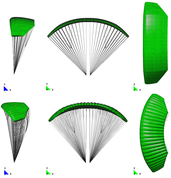
Coupled with a potential flow solver, the code has been used to simulate a high-performance parachute for delivery of heavy payloads. The canopy was designed and manufactured by CIMSA in the framework of the FASTWing Project [10]. The model contains an unstructured distribution of 11760 triangular elements (8824 for the aerodynamic surfaces exposed to the wind and 2936 for the internal ribs) and 11912 cable elements to model the suspension and control lines as well as the reinforcement tapes integrated into the canopy. The simulation is initialized with a partially inflated parachute configuration. The aerodynamic loads are updated as the simulation proceeds until a stable configuration is reached. Fig. 15 shows the change in shape from the beginning of the simulation to the equilibrium configuration.

Fig. 15 - Fastwing parachute. Initial configuration and final deformed shape

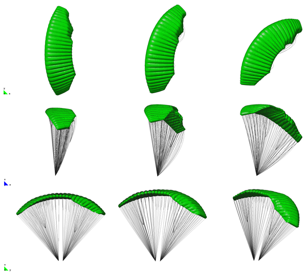
The code has also been used to predict the dynamic response of the parachute in order to simulate, for example, manoeuvres. The choice of an explicit scheme allows for instant transition from static to dynamic analysis if an unsteady flow solver is available. It must be stressed that the time step used by the structural solver is very short while for most applications the high-order modes of the mechanical response are of little relevance. Therefore it is not necessary to update the aerodynamic loads at every step in order to obtain a satisfactory global response. This saves processing time on the part of the flow solver. Fig. 16 illustrates a right turn manoeuvre.

Fig. 16 – Fastwing parachute right turn manoeuvre. Starting from the steady state the right brake is pulled. Yaw angle increases form left to right

6.2 Drag canopy deployment

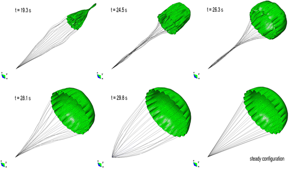
This is a simple inflation test aimed at exploring the capabilities of the code to simulate parachute deployment and inflation. Direct calculation of the pressure field around the partially inflated canopy is an extremely challenging task. Therefore, semi-empirical correlations have been used for the pressure field. Deployment takes place in two steps. Initially the apex of the canopy is pulled in the direction of the incident wind. Once the lines and canopy have been stretched the inflation phase begins. The parachute is discretized with an unstructured grid of 3390 triangular elements and 2040 cable elements modelling the suspension lines and fabric reinforcements. Fig. 17 shows the inflation stage, including the final steady configuration.

Fig. 17 – Several stages of the parachute deployment

6.3 Draping simulation

By virtue of the wrinkling model the code is able to simulate the interaction between flexible fabrics and rigid objects. In the example shown a square membrane 3m across is released on top of a rigid circular disc with a diameter of 2m. The fabric is subject to the action of gravity, contact forces and damping forces introduced to simulate the effect of the air. The definition of the rigid surface is analytic so it does not need to be discretized (i.e. it does not enter the mesh). The membrane has been meshed with an unstructured grid of 8262 elements. The complete process, 4s of real time, can be simulated in just 9s in a current mid-range desktop computer. Fig. 18 shows several snapshots of the process.

Fig. 18 - Draping simulation. Snapshots taken every 0,4s

6.4 Blast loading of inflatable structures

In recent times, use of inflatable structures as shelters against blast waves and even as a means of containing the effects of explosions has become a topic of interest. In order to address this kind of problem an additional material model has been incorporated in the code which allows for simulation of the propagation of pressure perturbations on air. An equation of state model has been used together with the tetrahedral elements in order to asses the blast wave attenuation which takes place across the inflatable structure. The events being simulated involve extremely short time scales during which the distances travelled by most nodes of the mesh are not large compared with the general dimensions of the structure. Thus, a lagrangian formulation for the air is acceptable, at least for those volumes not directly exposed to the effect of the blast. This is the case for the air contained inside the structure and for those parts of the atmosphere shielded from the explosion. Assuming an ideal gas which evolves in an isentropic way, the relation between pressure and density is:

${\frac {p}{{\rho }^{\gamma }}}={\frac {p_{0}}{{\rho }_{0}^{\gamma }}}$

(6.1)

where the subindex 0 denotes some reference conditions (e.g. initial conditions) and γ is the ratio of specifics heats of the gas. The pressure at any time is therefore obtained from

$p=p_{0}{\left({\frac {\rho }{{\rho }_{0}}}\right)}^{\gamma }=$$p_{0}{\left({\frac {{\Omega }_{0}}{\Omega }}\right)}^{\gamma }$

(6.2)

It is thus possible to calculate the pressure using the initial conditions and the change in volume of the element. This information is available from (4.56). The speed of sound in the medium is given by

$c^{2}=\gamma {\frac {p}{\rho }}$

(6.3)

An equivalent bulk stiffness for the air can be obtained from (6.3) by defining

$c^{2}={\frac {K_{eq}}{\rho }}{\mbox{ }}{\mbox{ }}{\mbox{ }}\Rightarrow {\mbox{ }}{\mbox{ }}{\mbox{ }}K_{eq}=$$\gamma p$

(6.4)

The parameter Keq is an estimate of the volumetric stiffness of the air. A gas has no shear stiffness so excessive mesh distortions could appear if only the pressure term (6.2) were included into the material response for those elements modelling air. To counter this problem some level of numerical shear stiffness is added to the formulation in order to control mesh distortion while not affecting the overall properties of the solution. To this effect this stabilizing term is defined as:

$G_{num}=\delta K_{eq}{\mbox{ }}{\mbox{ }}{\mbox{ }}{\mbox{ }}{\mbox{ }}{\mbox{ }}\left(\delta <<1\right)$

(6.5)

The parameter δ must be kept small in order to prevent excessive accumulation of energy in the form of shear deformation. The complete material response (including the shear stabilization term) is then given by

${\boldsymbol {\sigma }}=2G_{num}{\boldsymbol {e}}-p_{0}{\left({\frac {{\Omega }_{0}}{\Omega }}\right)}^{\gamma }{\boldsymbol {I}}$

(6.6)

The stability limit for the gas elements is calculated in the usual way (2.30) using (6.3) as the characteristic wave sped. As the speed of sound in air is much smaller that the wave speeds in solids, the air elements are not usually a limiting factor (except in cases of severe element distortion).

The example presented corresponds to a conceptual design for a blast containment device. The overall dimensions of the structure are 16x11x4,5m. Due to the double symmetry only a quarter of the geometry has been modelled. The mesh contains 2376000 tetrahedral elements and 79440 triangular membrane elements. The volume elements are located inside the cells of the structure and in the surrounding atmosphere. The volume of atmosphere meshed extends 9m outside the structure (see Fig. 19).

Fig. 19 – Computational domain geometry. Structure shown in dark grey and surrounding atmosphere in light gray

The pressure field corresponding to the explosion of a charge of 10kg of TNT has been computed with an Euler flow solver and used as prescribed load history on the inner wall of the structure. In a regular desktop computer the code is able to advance 10 time steps approximately every 9s. Given to short time scales involved (the time it takes for the shockwave to leave the domain is on the order of 10ms) the CPU time for a complete simulation is in the neighbourhood of 10 minutes (the exact value depends on the particular conditions of each simulation, as the stability limit changes as the mesh deforms). The explicit algorithm proves itself extremely efficient when dealing with fast transient events. Fig. 20 shows four snapshots of the temporal evolution of the structural deformations.

Fig. 20 - Inflatable structure subject to blast loading. Time between frames: 2ms

7 Conclusions

The theoretical background as well as details of implementation of an explicit dynamic structural solver (PUMI_MEM) have been presented. The software was developed as part of a broader effort to build a coupled fluid-structural analysis package for parachute simulations. The code was designed to obtain robust solutions of the highly nonlinear behaviour of structural membranes. The severe convergence problems due to the statically indeterminate behaviour of the structure where overcome by performing a dynamic simulation (even when only the static solution is sought). To counter the limitations imposed by the large changes in geometry expected an explicit time integration scheme was chosen. While this limits the allowable time step, issues related to the limited convergence radius of implicit schemes are completely eliminated. Even if the time step limitation might seem problematic at first, the very lost cost per iteration more than overcomes this issue. Another important characteristic of thin membranes is their virtually zero compression strength due to wrinkling. This has to be accounted for in order to obtain realistic solutions. As there is no global stiffness matrix to assemble in the explicit method, implementation of a wrinkling model is straightforward. Only the constitutive law has to be changed to include no-compression behaviour. Several benchmarks have been presented showing the accuracy of the results in situations where the geometrical nonlinearities and the asymmetry of the material response are determinant. The choice of a dynamic solver also enables study of the system’s transient response with no changes to the code. Examples of application to parachute deployment and manoeuvres have been presented. While initial focus was on parachute simulation, applications to other fields of technological interest have been tested. In all cases the code has shown an excellent performance in terms of CPU time.

Acknowledgements

The authors wish to thank the support from CIMSA Ingeniería y Sistemas [15] for providing sample parachute geometries as well as experimental measurements used during the development of the code.

References

[1] E. Ortega, R. Flores and E. Oñate. Innovative numerical tools for the simulation of parachutes. CIMNE publication, PI341, 2010.

[2] E. Ortega, R. Flores and E. Oñate. A 3D low-order panel method for unsteady aerodynamic problems. CIMNE publication, PI343, 2010.

[3] R. Rossi. Light weight structures: Structural analysis and coupling issues. PhD thesis, University of Bologna, 2005.

[4] J. Drukker and. D.G. Roddeman. The wrinkling of thin membranes: Part 1 -theory. Journal of Applied Mechanics, 54:884–887, 1987.

[5] J. Drukker and. D.G. Roddeman. The wrinkling of thin membranes: Part 2 - numerical analysis. Journal of Applied Mechanics, 54:888–892, 1987.

[6] R. Rossi, R. Vitaliani. Numerical coupled analysis of flexible structures subjected to the fluid action. In 5^th PhD symposium, Delft, 2004.

[7] T. Belytschko, W.K. Liu, and B. Moran. Nonlinear finite elements for continua and structures. John Wiley & Sons, 2000.

[8] O.C. Zienkiewicz and R.L Taylor. The finite element method, Volume I. Butterworth-Heinemann, 2000.

[9] R.L. Taylor. Finite element analysis of membrane structures. Technical report, CIMNE, 2001

[10] R. Rossi. A finite element formulation for 3D membrane structures including a wrinkling modified material model. Technical Report 226, CIMNE, 2003.

[11] R.M. Pauletti, D.M. Guirardi and T.E. Deifeld. Argyri’s natural membrane finite element revisited. Proceedings of the International Conference on Textile composites and Inflatable Structures, Barcelona, 2005.

[12] P. Contri and B.A. Schrefler. A geometrically nonlinear finite element analysis of wrinkled membrane surfaces by a no-compression material model. Communications in applied numerical methods, 4:5–15, 1988.

[13] R. Ziegler, W. Wagner and K. Bletzinger. A multisurface concept for the finite element analysis of wrinkled membranes. Proceedings of the 4^th International colloquium on computation of shell & spatial structures, IASS – IACM, 2000.

[14] J. Hornig. Analyse der Faltenbildung in Membranen aus unterschiedlichen Material. PhD thesis, Technischen Universität Berlin, 2004.

[15] CIMSA Ingeniería y Sistemas. Web page: http://www.cimsa.com/ (checked February 8^th 2011).