Design and optimization of a self-deployable composite structure

1 Symbols and Abbreviations

CNC	Computer Numerical Control
ESA	European Space Agency
FEA	Finite Element Analysis
GA	Genetic Algorithm
MARSIS	Mars Advanced Radar for Surface and Ionosphere Sounding
PSO	Particle Swarm Optimization
${\mathit {\boldsymbol {A}}}$	Ply angle
${\mathit {\boldsymbol {C}}}_{\mathit {\boldsymbol {0}}}$	Coefficient of inertia
${\mathit {\boldsymbol {C}}}_{\mathit {\boldsymbol {1}}}$	Coefficient of cognitive behavior
${\mathit {\boldsymbol {C}}}_{\mathit {\boldsymbol {2}}}$	Coefficient of social behavior
${\mathit {\boldsymbol {E}}}_{\mathit {\boldsymbol {11}}}$	Young’s modulus in the direction 11
${\mathit {\boldsymbol {E}}}_{\mathit {\boldsymbol {22}}}$	Young’s modulus in the direction 22
${\mathit {\boldsymbol {G}}}_{\mathit {\boldsymbol {12}}}$	Shear modulus in the direction 12
${\mathit {\boldsymbol {IF}}}$	Index of failure
${\mathit {\boldsymbol {P}}}$	Penalty factor
${\mathit {\boldsymbol {Perf}}}$	Performance value
${\mathit {\boldsymbol {P}}}_{\mathit {\boldsymbol {n}}}$	Number of plies
${\mathit {\boldsymbol {R}}}_{\mathit {\boldsymbol {i}}}$	Internal radius of the composite tube
${\mathit {\boldsymbol {R}}}_{\mathit {\boldsymbol {1}}}{\mathit {\boldsymbol {,\,}}}{\mathit {\boldsymbol {R}}}_{\mathit {\boldsymbol {2}}}$	Radius of the left or right circle of the slot
${\mathit {\boldsymbol {R}}}_{{\mathit {\boldsymbol {1}}}{\mathit {\boldsymbol {r}}}}{\mathit {\boldsymbol {,\,}}}{\mathit {\boldsymbol {R}}}_{{\mathit {\boldsymbol {2}}}{\mathit {\boldsymbol {r}}}}$	Ratio between the width of the slot and ${\textstyle {R}_{1}}$ or ${\textstyle {R}_{2}}$
${\mathit {\boldsymbol {SD}}}$	Slot’s displacement relatively to the longitudinal axis of the tube
${\mathit {\boldsymbol {SL}}}$	Slot’s length
${\mathit {\boldsymbol {\nu }}}_{\mathit {\boldsymbol {12}}}$	Poison’s coefficient in the direction 12
${\mathit {\boldsymbol {\nu }}}_{\mathit {\boldsymbol {23}}}$	Poison’s coefficient in the direction 23
${\mathit {\boldsymbol {X}}}_{\mathit {\boldsymbol {t}}}$	Longitudinal tensile strength
${\mathit {\boldsymbol {X}}}_{\mathit {\boldsymbol {c}}}$	Longitudinal compressive strength
${\mathit {\boldsymbol {Y}}}_{\mathit {\boldsymbol {t}}}$	Transverse tensile strength
${\mathit {\boldsymbol {Y}}}_{\mathit {\boldsymbol {c}}}$	Transverse compressive strength

2 Introduction

In spacecraft design, one of the major constraints is the capability of the launcher, considering both size and total mass. Designs that are based on large, rigid structures are constrained in size by the dimensions of the fairing. At the same time, developing launchers capable of sending larger payloads is an extremely difficult task. Given this scenario, adopting deployable structures, capable of changing their configuration from a packed and compact form to a large and deployed state once the payload is in orbit, is a highly attractive solution [1]. First, metallic solutions were developed and then upgraded to lighter composite systems that deploy by releasing the strain energy stored during the compaction process [2], [3]. Well-known applications of this concept are the elastic-hinges included in the monopole and dipole antennas of MARSIS (Mars Advanced Radar for Surface and Ionosphere Sounding), which allowed the folding of antennas with lengths up to 20 meters [4] (Figure 1 and Figure 2, respectively).

Figure 1. Functioning of an elastic-hinge (adapted from [5]).

Figure 2. Monopole and dipole antennas of MARSIS (adapted from [6]).

However, deployable structures have two opposing requirements: flexibility to sustain high strain deformations and rigidity to support external loads and/or reach certain natural frequencies [2]–[4], [7]–[11].

Numerical models that predict the stress-strain state of the material have aided the design of these structures, which require high strain capability and damage tolerance [5], [12], [13]. Despite the fact that designs that minimize the damage installed in the structure have been reported in the literature, a geometry that does not initiate damage during operation while meeting frequency requirements has not been found [4]. As an example, the experimental validation of the antennas of MARSIS, designed to have a natural frequency higher than 0.05Hz, reports “no significant damage to the fully flight representative hardware” [4].

Furthermore, in recent years, the European Space Agency (ESA) considered that telecommunication satellites could employ this technology. Once again, the objective is to replace mechanical arms with a lighter solution. However, the antennas of these satellites require a natural frequency higher than 1.0Hz, 20 times above the requirements of MARSIS [14], and 100 times higher than the natural frequency obtained by implementing solutions available in the literature [5]. This increases the difficulty of meeting the opposing requirements that characterize deployable structures and their applications.

3 Framework

Given the difficulties involved in the design of deployable structures, the increasing requirements and their potential use, this paper aims at applying optimization algorithms to find an optimal solution of an elastic-hinge capable of meeting damage and frequency requirements.

During this research, numerical models capable of estimating the natural frequency and the structural integrity of the structure were implemented. The structural model was experimentally validated using a representative specimen of the elastic-hinge, comparing the numerical and experimental folding behavior and the forces involved in the process. The experimental validation of the natural frequency model was performed and reported in [15], therefore, it was not repeated in this investigation.

The numerical models were integrated in an optimization process that used them to estimate the frequency and structural behavior of possible elastic-hinge designs. The optimization process was divided in two section: first, a global and discrete search that utilized a genetic algorithm (GA), then, a local and continuous search through a particle swarm optimization (PSO) method. A meta-optimization process was used in an attempt to find the most suitable internal parameters for the aforementioned optimization algorithms.

The approach was validated experimentally. However, the output obtained did not comply with the design requirements. Therefore, a second iteration of the slot hinge geometry was investigated numerically and the results discussed.

4 Design Requirements

In this research, the deployable structure considered is a composite arm with two integrated elastic-hinges. Each end of the arm should be connected to the satellite and to an antenna, respectively. Figure 3 best describes the application.

Figure 3. Description of the deployable system considered in this research.

The design requirements include geometric and functional requisites. From a functional point of view, the deployable structure should have a natural frequency higher than 1.0Hz and should not initiate damage during operation. In this research, the damage requirement is evaluated by means of different failure criteria: Hashin’s failure criteria, Azzi-Tsai-Hill, Tsai-Hill, Tsai-Wu and Maximum Stress. It is assumed that no damage has initiated during operation if the maximum index of every failure of these criteria is lower than 1.0. From a geometric perspective, it is imposed that the arm should have a circular cross-section, whose diameter cannot exceed 200.0mm.

These requirements correspond to the minimum requirements for this application, as reported in [14]. To obtain a more robust solution, a safety factor of 10% was applied to the frequency and damage requirements. This implies that the natural frequency should be higher than 1.1Hz and that the index of failure must be lower than 0.9 for all the criteria under assessment.

Additionally, it is assumed that the location of the elastic-hinges in the deployable arm is fixed and that the antenna to be attached on its free-end has a mass of 27kg. The center of mass of the antenna is located at 1.4m away from the tip of the arm.

As a result of these restrictions, the modifiable parameters are: the radius of the arm, the material, number of plies, ply-orientation and the geometry of the slot that characterizes the elastic-hinge.

5 Numerical Details

Finite element analysis was carried out to estimate the natural frequency and structural integrity of the system, using ABAQUS^®. In this section, the implemented numerical models are described. Both models consider a parametrization of the modelled geometry, which is described in detail in section 7.1, allowing an easy modification of the numerical models.

5.1 Natural Frequency Model

The natural frequency finite element model considers the integrated system composed by the composite arm with two elastic-hinges and the antenna attached to its free-end.

The antenna is represented as a point mass of 27kg, located 1.4m away from the tip of the composite arm and connected to it through a beam multi-point constraint. The other end of the composite arm is fixed, representing its attachment to the satellite. Figure4 represents these boundary conditions applied to a generic antenna arm.

Figure 4. Highlight of the boundary conditions considered in the natural frequency model.

The deployable arm was modelled with three-dimensional deformable shell elements with 4 nodes (S4R in ABAQUS^®) and reduced integration. Each element had an average size of 2.5mm. The material properties introduced in the numerical model are summarized in Table 1.

The natural frequency is determined using a linear perturbation analysis, which applies the Lanczos algorithm. This approach has been used several times in the literature to estimate the natural frequency of similar deployable structures [5], [12], [16] and even some different concepts [17]. It has been experimentally validated in [15], reporting an error of 6% between numerical and experimental results for the first natural frequency and 20% for the higher order frequencies.

Since the objective of the natural frequency model is to estimate the first natural frequency of the system and that an error of only 6% was observed through experimental validation, the numerical model is considered suitable for this investigation.

This numerical model considers a parametrization of the geometry of the structure, allowing an easy modification of the geometry of the modelled structure

5.2 Structural Model

The structural model considers a segment of the composite arm, corresponding to only one elastic-hinge. Similarly to the natural frequency model, three-dimensional deformable shell elements with 4 nodes (S4R in ABAQUS ^®) and reduced integration were used to model the elastic-hinge. Nonetheless, to reduce the computational cost of the finite element model, the elastic-hinge was divided in three regions, as shown in Figure 5.

Figure 5. Highlight of the different regions considered in the structural model. Each region is represented with a different colour (blue, dark-grey and light-grey) and has a different mesh size.

The central region, highlighted with a light-grey colour, corresponds to the area where the slot of the elastic-hinge is located and where the highest stress concentration occurs. Therefore, the numerical model considers the existence of a composite layup feature with multiple plies in this region, allowing a more detailed analysis of the stress and strain state of each element. The elements in this region had an approximate size of 2.5mm.

The other two regions do not sustain significant stresses or strains. This fact makes them only relevant for the analysis of the folding and deployment behaviours of the elastic-hinge to capture the full component rigidity behaviour when solicited. Since their stress and strain states are not significant from a design point of view, they were modelled as a single layer of elements with the homogenized properties of the composite. This procedure reduces the number of calculations in the model and, therefore, the computational time. The elements in the blue region had an approximate average size of 4mm, while the elements in the dark-grey region create a transition between both neighbour meshes.

In order to replicate the experimental testing equipment, the applied boundary conditions consider the existence of two holders, responsible for supporting the ends of the composite arm. An angular rotation is applied, forcing the arm to fold, and two plates, that pinch the tapes of the elastic hinge, force them to bend before the folding of the component starts. These boundary conditions are in accordance with [5] and represented in Figure 6.

Figure 6. Visual representation of the three folding steps (image adapted from [5]).

6 Validation of the Structural Model

The structural model was validated experimentally by comparing the experimental and numerical torque-angle curves. These curves indicate the total torque that is applied at the ends of the elastic-hinge to fold it, as a function of the folding angle, and were first used as a validation method in [13] and [18].

The following sections describe in detail the materials used, geometry of the specimens, experimental setup, calibration procedure and output comparison.

6.1 Materials and Specimens

The material considered in this research was AS4/8552, an unidirectional carbon/epoxy system provided by Hexcel. The mechanical properties implemented in the models are summarized in Table 1.

Table 1. Elastic and strength properties of AS4/8552, according to [19] and [20], respectively

	Property	Value	Unit
Elastic properties	${E}_{11}$	128	GPa
	${E}_{22}$	7625	MPa
	${\nu }_{12}$	0.35	-
	${\nu }_{23}$	0.45	-
	${G}_{12}$	4358	MPa
Strength properties	${X}_{t}$	2300	MPa
	${X}_{c}$	1200	MPa
	${Y}_{t}$	100	MPa
	${Y}_{c}$	220	MPa
	${S}_{L}$	100	MPa

The geometry of the specimens used in the experimental validation is described by Figure 8. This geometry consists on a tubular structure with two 0.18125mm thick plies oriented at +/- 45º, an internal diameter of 39mm and a cut-out, defining the slot of the elastic-hinge.

Figure 7. Test rig used for measure the torque as a function of the folding angle.

Figure 8. Geometry of the specimen used for the experimental validation of the structural model.

Each specimen was manufactured by hand lay-up and cured in an autoclave according to the manufacturer specifications. Then, the slot was cut using a CNC machine.

6.2 Experimental Setup and Procedure

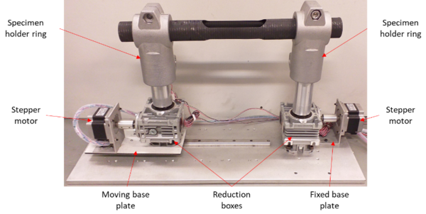
The torque necessary to fold the elastic-hinge as a function of the folding angle was used to validate the numerical model. A custom test rig (Figure 7) was developed based on the work described in [13], [18]. The rig consists of two sets of holders that support the composite tube, and are able to apply torsion at both ends of the tube.

The torsion is controlled by the movement of two stepper motors. One of the stepper motors is fixed to the base of the machine, allowing the holder to rotate only around a fixed axis. The other motor is fixed to a moving base, allowing the holder to rotate while moving along a linear track. Figure 7 shows the mechanism.

The torque measurement is made using a ±45º strain gauge attached to the shaft of the specimen holder ring. The strain gauge in connected to a signal amplifier HX711, that delivers the information to a User Interface using an Arduino based microcontroller.

Before testing, each holder is calibrated. The calibration procedure consists on fixing a rod, with a known length, to the holder and placing a calibrated weight on its end (Figure 9). The torque is determined mathematically and the output from the electronic system is recorded. The next step is to place, in the same location, another calibrated weight, so the system output can be sensed and recorded. This step has to be repeated until the estimated torsion value is reached corresponds to that of the calibrated weights. Once all the data is collected, a simple linear, quadratic or higher order regression has to be applied to fit the data and obtain the torque equation for this particular system.

Figure 9. Calibration method using a rod and a calibrated weight.

6.3 Output Comparison

The experimental procedure was repeated for three valid experiments, with different test specimens. A representative curve of the torque-angle measurement is shown in Figure 10 and compared to the numerical prediction, revealing a good agreement between both results. It is possible to observe some irregularities in the experimental curve, which do not exist in the numerical prediction. This difference is caused by the use of the two stepper motors, which do not allow a continuous movement, but rather a movement caused by a series of small increments. This factor, in conjunction with the existence of friction, causes some irregularities in the experimental torque-angle curve. The maximum torque values observed during the different experimental tests are reported in Table 2, indicating consistent results with an average deviation of 0.06.

Figure 10. Torque applied to an elastic-hinge as a function of the folding angle.

Table 2. Maximum torque according to experimental and numerical results

		Maximum torque (N.m)
Experimental results	Sample 1	5.25
	Sample 2	5.33
	Sample 3	5.16
	Average	5.25
	Average deviation	0.06
Numerical results		5.14

7 Design and Optimization

This section describes the design and optimization process of the composite deployable arm, including: the design variables, objective function, selected optimization algorithms, internal parameters selected for each algorithm and an analysis of the obtained outputs.

Section 7.1 describes the design variables used. This includes a description of the possible geometries that can be obtained, by means of the selected parametrization, and a definition of the design space.

The description of the objective function (section 7.2) explains how the information obtained from the numerical models is utilized to explore and improve possible solutions.

The section dedicated to the optimization process (7.3) explains how a genetic algorithm and a particle swam optimization method were combined. In this integration, advantage was taken from their respective discrete and continuous natures to develop an optimization process divided in a global and local search. This enables a quick overview of the design space, followed by a detailed search in the neighbourhood of the most promising solution.

Finally, the last section (Erro! A origem da referência não foi encontrada.) reports the process used to select the internal parameters of the optimization algorithms.

7.1 Design Variables

The considered design variables define the geometry of the slot and of the composite arm as a combination of geometrical figures. This parametrization, described in Figure 11, is inspired in the work reported in [13] but allows a larger number of possible designs and the inclusion of asymmetries, as shown in Figure 12.

Figure 11. Visual representation of the design variables that define the geometry of the slot of the elastic-hinge.

Figure 12. Examples of possible geometries considered by the parametrization used.

In total, nine design variables were considered. These include the number of plies of the composite ${\textstyle \left({P}_{n}\right)}$ , ply angle ${\textstyle \left(A\right)}$ and the following geometric variables:

* ${\textstyle {\mathit {\boldsymbol {R}}}_{\mathit {\boldsymbol {i}}}}$ – Internal radius of the tube.

* ${\textstyle {\mathit {\boldsymbol {R}}}_{\mathit {\boldsymbol {1}}}}$ and ${\textstyle {\mathit {\boldsymbol {R}}}_{\mathit {\boldsymbol {2}}}}$ – Radius 1 and 2, defined as a percentage of ${\textstyle {\mathit {\boldsymbol {R}}}_{\mathit {\boldsymbol {i}}}}$;

* ${\textstyle {\mathit {\boldsymbol {R}}}_{{\mathit {\boldsymbol {1}}}{\mathit {\boldsymbol {r}}}}}$ and ${\textstyle {\mathit {\boldsymbol {R}}}_{{\mathit {\boldsymbol {2}}}{\mathit {\boldsymbol {r}}}}}$ – Ratio between the slot’s width and ${\textstyle {\mathit {\boldsymbol {R}}}_{\mathit {\boldsymbol {1}}}}$ or ${\textstyle {\mathit {\boldsymbol {R}}}_{\mathit {\boldsymbol {2}}}}$ on the center of each circle (visually described by ${\textstyle {W}_{1}}$ and ${\textstyle {W}_{2}}$, where ${\textstyle {W}_{n}=}$${R}_{n}\times {R}_{nr}$, with ${\textstyle n=1,2}$);

* ${\textstyle {\mathit {\boldsymbol {SL}}}}$ – Slot’s length, defined as the product of a scalar and ${\textstyle {\mathit {\boldsymbol {R}}}_{\mathit {\boldsymbol {i}}}}$;

* ${\textstyle {\mathit {\boldsymbol {SD}}}}$ – Slot’s displacement from the longitudinal axis of the tube. Defined as a percentage of the largest value between ${\textstyle {\mathit {\boldsymbol {R}}}_{\mathit {\boldsymbol {1}}}}$ and ${\textstyle {\mathit {\boldsymbol {R}}}_{\mathit {\boldsymbol {2}}}}$;

Each variable has the following minimum and maximum value, shown in Table 3. These variables were mainly defined as percentages and ratios to ensure that the algorithm cannot generate impossible solutions by combining incompatible design values. An example of an impossible solution would be a slot with ${\textstyle {R}_{1}}$ larger than ${\textstyle {R}_{i}.}$ Avoiding these unrealistic cases leads to a simpler design space and a higher probability of success in finding the global optimum.

Table 3. Maximum and minimum values of each design variable

Variable	Minimum	Maximum	Unit
${\mathit {\boldsymbol {R}}}_{\mathit {\boldsymbol {i}}}$	20	100	mm
${\mathit {\boldsymbol {R}}}_{\mathit {\boldsymbol {1}}}{\mathit {\boldsymbol {,\,}}}{\mathit {\boldsymbol {R}}}_{\mathit {\boldsymbol {2}}}$	15	80	%
${\mathit {\boldsymbol {R}}}_{{\mathit {\boldsymbol {1}}}{\mathit {\boldsymbol {r}}}}{\mathit {\boldsymbol {,\,}}}{\mathit {\boldsymbol {R}}}_{{\mathit {\boldsymbol {2}}}{\mathit {\boldsymbol {r}}}}$	0.1	1.0	-
${\mathit {\boldsymbol {SL}}}$	3	10	-
${\mathit {\boldsymbol {SD}}}$	0	100	%
${\mathit {\boldsymbol {P}}}_{\mathit {\boldsymbol {n}}}$	1	4	pair(s)
${\mathit {\boldsymbol {A}}}$	0	90	º

7.2 Objective Function

The design process of the composite deployable arm considers geometrical, damage and frequency requirements. The geometrical requirements, such as the diameter, which cannot exceed 200.0mm, can be addressed by restraining the domain of the design variable(s), as described in section 7.1. The frequency requirement can be seen as another constraint, where solutions whose natural frequency is lower than 1.0Hz are rejected. These two considerations leave the minimization of the installed damage as the only objective of the optimization process and avoids the use of multi-objective optimization processes where the complexity is far greater.

With this strategy in mind, the objective function was defined as the minimization of damage, where the damage installed in each possible design was estimated using the structural numerical model described in section 5.2. However, executing a structural analysis on every possible solution would lead to an exceedingly large computational cost. To avoid such situation, each candidate solution had its natural frequency estimated through the numerical model described in section 5.1. If the natural frequency of a possible solution was larger than 1.1Hz and lower than 1.25Hz, it would be evaluated through a structural analysis and its performance value ${\textstyle \left(Perf\right)}$ set equal to the maximum index resulting from the application of the failure criteria included in the numerical model (listed in section 4). If the natural frequency was not within this range, the performance value was set equal to a penalty factor ${\textstyle \left(P\right)}$ and the structural analysis skipped. Equation (1) shows the formula used to determine the performance value of a solution, while Figure 13 shows a graphic representation of the penalty factor as a function of the natural frequency.

${\textstyle \left\{{\begin{matrix}Perf=15,\quad \,\,0.0\leq f<1.0\,\vee 1.25<f\leq 1.5\,\\Perf=12,\quad \,\,1.0\leq f<1.1\\{\begin{matrix}Perf=Max\left(IF\right),\quad \,1.1\leq f\leq 1.25\\Perf=20,\quad \,1.5<f<+\infty \end{matrix}}\end{matrix}}\right.}$ $(1)$

Where ${\textstyle Max\left(IF\right)}$ is the largest index of failure of the failure criteria included in the structural analysis (listed in section 4).

Figure 13. Graphic representation of the penalty factor as a function of the natural frequency of the design considered.

Solutions whose natural frequency was lower than 1.1Hz received a penalty factor for not meeting the frequency requirement. This penalty was more severe for solutions whose natural frequency was lower than 1.0Hz, since they were further away from the minimum requirement. The penalty applied to solutions with a natural frequency above 1.25Hz is justified by the proportionality between the stiffness of a structure and its natural frequency. The increase in natural frequency implicates an increase in stiffness, making the structure less flexible and less likely to fold without initiating damage. Even more severe penalties were applied to solutions with a frequency larger than 1.5Hz, for the same reason.

7.3 Optimization Process

The optimization process considered two different optimization algorithms: a genetic algorithm, inspired by the theory of natural selection [21], [22] and a particle swarm optimization method, a heuristic search method inspired by the collaborative behavior of biological populations [23]. Considering the classic implementation of these algorithms, it is possible to classify the GA as naturally discrete and the PSO as naturally continuous. The implication of this nature is that a classic GA is more suitable to optimize discrete variables and that a classic PSO is more suitable to optimize continuous variables. Given these characteristics, the optimization process was divided into a global and a local search.

The GA was applied during the global search, where only discrete values of each design variable were considered. This decision led to a reduction in the number of possible solutions that the optimization algorithm had to explore. Once a solution was found, the local search initiated. The local search consisted of applying the PSO method to search for an optimal solution in the neighbourhood of the solution found during the global search. The local search domain was defined by a ${\textstyle \pm 10\%}$ variation of each design variable, except for the number of plies, which was not included in the local search. This sequence of operations allows for a quick survey of the design space, followed by a more refined search near the optimum found.

8 Results and Discussion

Through multiple optimization attempts, it was observed that the best solutions found in each attempt usually had large slot radiae ${\textstyle \left({R}_{1},\,{R}_{2}\right)}$ and smaller widths ${\textstyle \left({R}_{1r},{R}_{2r}\right)}$ . Cases a), b) and c), shown in Figure 14, are examples of this scenario. However, these solutions did not meet the design requirements due to their maximum indexes of failure being 2.01, 2.04 and 2.05, respectively. Further evaluation of the geometries generated by the optimization algorithm led to the discovery of case d), which is also representative of this situation and corresponds to the solution with a lower index of failure (1.86), but did not to meet the natural frequency requirement (0.57Hz).

The best result obtained through the optimization process is shown in Figure 14 e) and has a maximum index of failure of 1.63, according to the Hashin’s failure criteria for matrix under compression, and a natural frequency of 1.22Hz. However, despite having a natural frequency higher than 1.1Hz, this solution fails to meet the damage requirements. The indexes of failure of this solution are shown in Table 4, while the design variables that define the geometry are shown in Table 5.

Figure 14. Best solutions found through the optimization processes. Cases b) and c) differ slightly in the slot’s width. Case d) has a lower index of failure (1.86) but does not meet the frequency requirement (0.57Hz). Case e) is the solution with the lowest index of failure (1.63) that meets the frequency requirements (1.22Hz).

Table 4. Indexes of failure observed according to each failure criterion

Criteria		Initial case
Azzi-Tsai-Hill		1.24
Hashin	Fibre compression	1.04
	Fibre tension	0.31
	Matrix compression	1.63
	Matrix tension	1.48
Maximum stress		1.22
Tsai Hill		1.25
Tsai Wu		1.40
Maximum index of failure		1.63

Furthermore, by analyzing the outputs of the structural models, it was possible to observe two main stress concentration regions, highlighted in red and orange in Figure 15. It was also observed that the amount of damaged material (red region) would decrease as the radius of the slot increased. The location of the stress concentration points, as well as the type of geometry found during the optimization process, is in agreement with the analysis reported in [13], [31], [32], which found similar designs through a parametric analysis.

Table 5. Variables defining the slot geometry used to compare the influence of the boundary conditions and of the removal of material. *Rounded value in mm, after obtaining the product between the percentage and ${\textstyle {\mathit {\boldsymbol {R}}}_{\mathit {\boldsymbol {i}}}}$.

Variable	Value	Unit
${\mathit {\boldsymbol {R}}}_{\mathit {\boldsymbol {i}}}$	85.0	mm
${\mathit {\boldsymbol {R}}}_{\mathit {\boldsymbol {1}}}$	35	%
${\mathit {\boldsymbol {R}}}_{\mathit {\boldsymbol {2}}}$	15	%
${\mathit {\boldsymbol {R}}}_{{\mathit {\boldsymbol {1}}}{\mathit {\boldsymbol {r}}}}$	0.35	-
${\mathit {\boldsymbol {R}}}_{{\mathit {\boldsymbol {2}}}{\mathit {\boldsymbol {r}}}}$	0.65	-
${\mathit {\boldsymbol {SL}}}$	480*	mm
${\mathit {\boldsymbol {SD}}}$	${\textstyle 4.0}$*	mm
${\mathit {\boldsymbol {P}}}_{\mathit {\boldsymbol {n}}}$	2	pair(s)
${\mathit {\boldsymbol {A}}}$	40	º

Additionally, it is noticeable that the solution with the lowest index of failure (case e) has an asymmetric design, which results in a stiffer region located on one end of the slot. This solution implies a direct relation between the boundary conditions, that define the folding process, and the installed damage initiation in the component. Therefore, the boundary conditions implemented in the folding process need to be revised in order for their effect in the damage initiation be minimized.

Figure 15. Highlight of the stress concentration zones. The regions marked in red have the largest failure indexes, followed by the orange region.

Based on these observations, it can be theorized that further improvements on the design, at the damage and frequency levels, of the elastic-hinge should be achieved by implementing two modifications. The first, concerning the boundary conditions. The loads installed on the edges of the tapes of the elastic hinge are the result of the rotations applied to each holder. Therefore, as an alternative, the folding process should consider the vertical displacement of the lowest tape, resulting in a reduction of compressive loads. The second modification involves the design variables in order for the optimization process of the slot geometry to consider possible removal of material from the stress concentration points highlighted in Figure 15.

9 Conclusion

This research consisted of the integration of finite element numerical models, used to estimate the structural performance and natural frequency of a deployable structure, in an optimization process that involved a genetic algorithm, for a global search followed by a particle swarm optimization method, for a local, more refined, search. Through this research, the following conclusions are summarized:

- The numerical results obtained from the structural analysis of the elastic-hinge were in good agreement with the experimental results.

- Analysis of the results obtained led to the identification of limitations of the design variables commonly used in the literature to design this type of structures. These variables do not include geometries that may minimize the stress installed in the deployable structure.

- A geometry capable of reaching a natural frequency of 1.22Hz and a maximum index of failure of 1.63 was found. This solutions meets the natural frequency requirement but initiates damage during operation, and therefore is rejected.

- It is observed that the folding process directly affects the damage installed. This is the result of a non-optimized folding process, which translates in large compressive loads observed in the elastic-hinge. An alternative folding process should allow the reduction of damage installed and further enable the use of this type of methodologies.

- Future work should look towards including geometrical modifications to the stress hotspot areas in the algorithm. This will allow the computational process to have an exponential new alternatives to test and provide a better assessment of the slot geometry as well as further optimize the damage onset and frequency. Therefore, fulfilling the restrict imposed design requirements.

Acknowledgements

Authors gratefully acknowledge the funding of Project NORTE-01-0145-FEDER-000022 - SciTech - Science and Technology for Competitive and Sustainable Industries, financed by Programa Operacional Regional do Norte (NORTE2020), through Fundo Europeu de Desenvolvimento Regional (FEDER).”

This research was supported by ESA through the ESA ARTES programme.

We thank our colleagues from INEGI, SONACA and ESA who provided insight and expertise that greatly assisted the research.

References

[1] L. Puig, A. Barton, and N. Rando, “A review on large deployable structures for astrophysics missions,” Acta Astronaut., vol. 67, no. 1–2, pp. 12–26, (2010).

[2] S. Ferraro and S. Pellegrino, “Self-Deployable Joints for Ultra-Light Space Structures,” in AIAA Spacecraft Structures Conference, pp. 0694–0707, (2018).

[3] M. Kroon et al., “Articulated Deployment System for Antenna Reflectors,” in Proc. 16th European Space Mechanisms and Tribology Symposium, Bilbao, (2015).

[4] G. W. Marks, M. T. Reilly, and R. L. Huff, “The lightweight deployable antenna for the MARSIS experiment on the Mars express spacecraft,” in 36th Aerospace Mechanisms Symp, (2002), pp. 183–196.

[5] H. M. Y. C. Mallikarachchi and S. Pellegrino, “Quasi-Static Folding and Deployment of Ultrathin Composite Tape-Spring Hinges,” J. Spacecr. Rockets, vol. 48, no. 1, pp. 187–198, (2011).

[6] N. Grumman, “Photo Release -- NASA’s Jet Propulsion Laboratory, Royal Aeronautical Society Recognize Northrop Grumman for Success in Space Deployables,” (2007). [Online]. Available: https://news.northropgrumman.com/news/releases/photo-release-nasa-s-jet-propulsion-laboratory-royal-aeronautical-society-recognize-northrop-grumman-for-success-in-space-deployables. [Accessed: 27-Nov-2018].

[7] L. T. Tan and S. Pellegrino, “Thin-Shell Deployable Reflectors with Collapsible Stiffeners: Experiments and Simulations,” AIAA J., vol. 50, no. 3, pp. 659–667, (2012).

[8] D. Piovesan, M. Zaccariotto, C. Bettanini, M. Pertile, and S. Debei, “Design and Validation of a Carbon-Fiber Collapsible Hinge for Space Applications: A Deployable Boom,” J. Mech. Robot., vol. 8, no. 3, pp. 031007–031018, (2016).

[9] C. Wu and A. Viquerat, “Natural frequency optimization of braided bistable carbon/epoxy tubes: Analysis of braid angles and stacking sequences,” Compos. Struct., vol. 159, pp. 528–537, (2017).

[10] X. Tong, W. Ge, Y. Zhang, and Z. Zhao, “Topology design and analysis of compliant mechanisms with composite laminated plates,” J. Mech. Sci. Technol., vol. 33, no. 2, pp. 613–620, (2019).

[11] P. Kumar, A. Saxena, and R. A. Sauer, “Computational Synthesis of Large Deformation Compliant Mechanisms Undergoing Self and Mutual Contact,” J. Mech. Des., vol. 141, pp. 012302–012313, (2019).

[12] H. M. Y. C. Mallikarachchi and S. Pellegrino, “Deployment Dynamics of Ultrathin Composite Booms with Tape-Spring Hinges,” J. Spacecr. Rockets, (2014).

[13] H. Mallikarachchi and S. Pellegrino, “Design and Validation of Thin-Walled Composite Deployable Booms with tape-Spring Hinges,” in 52nd AIAA/ASME/ASCE/AHS/ASC Structures, Structural Dynamics and Materials Conference, (2011).

[14] ESA, “Statement of Work AO8702 - Antenna Deployment Arm with Integrated Elastic Hinges,” (2016).

[15] M. Sakovsky, “Design and Characterization of Dual-Matrix Composite Deployable Space Structures.” California Institute of Technology, (2018).

[16] H. Mallikarachchi and S. Pellegrino, “Simulation of quasi-static folding and deployment of ultra-thin composite structures,” in 49th AIAA/ASME/ASCE/AHS/ASC Structures, Structural Dynamics, and Materials Conference, 16th AIAA/ASME/AHS Adaptive Structures Conference, 10th AIAA Non-Deterministic Approaches Conference, 9th AIAA Gossamer Spacecraft Forum, 4th AIAA Multidisciplinary Des, p. 2053, (2008).

[17] E. C. Borowski, “Viscoelastic Effects in Carbon Fiber Reinforced Polymer Strain Energy Deployable Composite Tape Springs,” (2017).

[18] C. Boesch, C. Pereira, R. John, T. Schmidt, K. Seifart, and J. M. Lautier, “Ultra light self-motorized mechanism for deployment of light weight reflector antennas and appendages,” in European Space Agency, (Special Publication) ESA SP, (2007).

[19] E. V González, P. Maimí, P. P. Camanho, A. Turon, and J. A. Mayugo, “Simulation of drop-weight impact and compression after impact tests on composite laminates,” Compos. Struct., vol. 94, no. 11, pp. 3364–3378, (2012).

[20] C. S. Lopes, P. P. Camanho, Z. Gürdal, P. Maimí, and E. V González, “Low-velocity impact damage on dispersed stacking sequence laminates. Part II: Numerical simulations,” Compos. Sci. Technol., vol. 69, no. 7–8, pp. 937–947, (2009).

[21] D. Whitley, “A genetic algorithm tutorial,” Stat. Comput., vol. 4, no. 2, pp. 65–85, (1994).

[22] M. Gen and R. Cheng, Genetic algorithms and engineering optimization, vol. 7. John Wiley & Sons, (2000).

[23] R. Hassan, B. Cohanim, O. De Weck, and G. Venter, “A comparison of particle swarm optimization and the genetic algorithm,” in 46th AIAA/ASME/ASCE/AHS/ASC structures, structural dynamics and materials conference, p. 1897, (2005).

[24] F. J. Lobo, C. F. Lima, and Z. Michalewicz, Parameter setting in evolutionary algorithms, vol. 54. Springer Science & Business Media, (2007).

[25] A. Corana and M. and C. Martini and S. Ridella, “Corrigenda: ‘Minimizing Multimodal Functions of Continuous Variables with the “Simulated Annealing” Algorithm,’” ACM Trans. Math. Softw., (1989).

[26] M. Jamil, X. S. Yang, and H. J. D. Zepernick, “Test Functions for Global Optimization: A Comprehensive Survey,” in Swarm Intelligence and Bio-Inspired Computation, (2013).

[27] M. Jamil and X.-S. Yang, “A Literature Survey of Benchmark Functions For Global Optimization Problems Citation details: Momin Jamil and Xin-She Yang, A literature survey of benchmark functions for global optimization problems,” Int. J. Math. Model. Numer. Optim., (2013).

[28] M. Clerc and J. Kennedy, “The particle swarm-explosion, stability, and convergence in a multidimensional complex space,” IEEE Trans. Evol. Comput., vol. 6, no. 1, pp. 58–73, (2002).

[29] R. Poli, J. Kennedy, and T. Blackwell, “Particle swarm optimization,” Swarm Intell., vol. 1, no. 1, pp. 33–57, (2007).

[30] B. D. Bunday, Basic optimisation methods. Edward Arnold London, (1984).

[31] H. M. Y. C. Mallikarachchi and S. Pellegrino, “Optimized Designs of Composite Booms with Tape Spring Hinges,” in 51st AIAA/ASME/ASCE/AHS/ASC Structures, Structural Dynamics, and Materials Conference 18th AIAA/ASME/AHS Adaptive Structures Conference 12th, (2010).

[32] H. M. Mallikarachchi, “Thin-walled composite deployable booms with tape-spring hinges.” University of Cambridge, (2011).

[33] D. E. Goldberg and J. H. Holland, “Genetic algorithms and machine learning,” Mach. Learn., vol. 3, no. 2, pp. 95–99, (1988).

[34] S. S. Rao, Engineering optimization: theory and practice. John Wiley & Sons, (2009).

[35] A. R. Parkinson, R. Balling, and J. D. Hedengren, “Optimization methods for engineering design,” Brigham Young Univ., vol. 5, p. 11, (2013).

[36] R. Eberhart and J. Kennedy, “Particle swarm optimization,” in Proceedings of the IEEE international conference on neural networks, vol. 4, pp. 1942–1948, (1995).

[37] M. R. Bonyadi, Z. Michalewicz, and X. Li, “An analysis of the velocity updating rule of the particle swarm optimization algorithm,” J. Heuristics, vol. 20, no. 4, pp. 417–452, (2014).

[38] J. Kennedy, “Particle swarm optimization,” Encycl. Mach. Learn., pp. 760–766, (2010).