A type-2 fuzzy system model for reducing bullwhip effects in supply chains and its application in steel manufacturing

Abstract

The purpose of this paper is to evaluate and reduce the bullwhip effect in fuzzy environments by means of type-2 fuzzy methodology. In order to reduce the bullwhip effect in a supply chain, we propose a new method for demand forecasting. First, the demand data of a real steel industry in Canada is clustered with an interval type-2 fuzzy ${\textstyle c}$ -regression clustering algorithm. Then, a novel interval type-2 fuzzy hybrid expert system is developed for demand forecasting. This system uses Fuzzy Disjunctive Normal Forms (FDNF) and Fuzzy Conjunctive Normal Forms (FCNF) for the aggregation of antecedents. An interval type-2 fuzzy order policy is developed to determine orders in the supply chain. Then, the results of the proposed method are compared with the type-1 fuzzy expert system as well as the type-1 fuzzy time series method in the literature. The results show that the bullwhip effect is significantly reduced; also, the system has less error and high accuracy.

Keywords

Supply chain management ; Fuzzy clustering ; Interval type-2 fuzzy hybrid system ; Demand forecasting ; Ordering policy ; Bullwhip effect

1. Introduction

Customer demand information is very important in supply chains because of the competitive nature of industries. So, each entity in a supply chain tries to gather the demand information of its downstream customers. Demands of the downstream customers are considered as orders for their upstream suppliers. When an end customer places an order, this order is amplified as it moves through the chain. Such a phenomenon is recognized and described by Forrester  [1] . He named this effect “demand amplification”, which is now known as the bullwhip effect  [2] . The next research is related to Sterman  [3] , who described this effect in a popular beer game.

Five reasons for bullwhip effect occurrence have been introduced by Lee et al.  [4]  and [5] . These reasons are: demand forecasting, order batching, price fluctuation, rationing and shortage gaming, and none-zero lead time. Metters  [6] , Baganha and Cohen  [7] , Chen et al.  [8] , and Campuzano et al.  [9] focused on demand forecasting. Kelle and Milne  [10] , and Lee and Wu  [11] studied order batching as one of the causes of the bullwhip effect. Pricing is considered by Özelkan and Cakanyıldırım  [12] as the other reason for bullwhip occurrence. Cachon and Lariviere  [13] studied shortage gaming. Agrawal et al.  [14] investigated the effect of information sharing and lead time on the bullwhip effect, as well as on hand inventory.

In some situations, we encounter vague information in supply chains, which is represented by linguistic terms. Fuzzy logic is a proper method to model and solve those linguistic problems. For the first time, Carlsson and Fuller  [15] used fuzzy logic in bullwhip effect problems. Fazel Zarandi et al.  [16] presented an intelligent agent-based system for reducing the bullwhip effect in supply chains, in which all demands, lead times, and ordering quantities are fuzzy variables. Other work in the area of bullwhip effects in fuzzy environments is related to Fazel Zarandi et al.  [17] and Campuzano et al.  [9] . Fazel Zarandi et al.  [17] used a multi-agent system for reducing the bullwhip effect. Campuzano et al.  [9] considered a system dynamics model with type-1 fuzzy estimations of demand.

In some situations, the information is too vague to model the problem with type-1 fuzzy sets. In type-2 fuzzy systems, each membership degree, itself, is represented by another membership degree, which is called the secondary membership  [18] . The method used for modeling and solving these kinds of problem is type-2 fuzzy theory, which was introduced by Zadeh  [19] . Turksen  [20] and Gorzalczany  [21] are pioneers of interval type-2 fuzzy sets. This fact that fuzzy normal forms can be generated from fuzzy truth tables has been presented by Turksen  [20] . Turksen  [22] introduced the Fuzzy Disjunctive Normal Form (FDNF) and the Fuzzy Conjunctive Normal Form (FCNF) for type-2 fuzzy sets, which are obtained from the fuzzy truth table. One controversial issue in type-2 fuzzy theory has been the complexity of the system. However, Sepúlveda et al.  [23] showed that interval type-2 fuzzy systems can accelerate the computation process and control uncertainty better than type-1 fuzzy systems. Moreover, Melin et al.  [24] showed that the most conspicuous images are obtained by using interval type-2 fuzzy systems. Interval type-2 fuzzy systems consist of three steps: structure identification, inference engine, and parameter tuning.

Rhee and Hwang  [25] , [26]  and [27] presented a Interval Type-2 Fuzzy ${\textstyle C}$ -Means clustering algorithm (IT2 FCM) for the structure identification phase of type-2 fuzzy systems. This method is used for Mamdani’s systems. However, the Fuzzy ${\textstyle C}$ -Regression clustering Model (FCRM) is utilized in the structure identification phase of Takagi–Sugeno’s systems.

In Mamdani’s systems, all variables in consequents and antecedents have linguistic variables. In contrast, T–S systems have linguistic variables, not in the consequent part, but in their antecedents. On the other hand, the consequent of a T–S system is a function. Therefore, they require different reasoning and structure identification techniques. Hidalgo et al.  [28] used the genetic algorithm for designing a type-2 fuzzy inference system with the Mamdani method.

Reviewing the literature of bullwhip problems shows that there is no research work on the bullwhip effect in type-2 fuzzy environments. So, this paper is the first to focus on bullwhip effect reduction, in which all demands, orders, and lead times are type-2 fuzzy sets. In order to model the problem, we extend a method introduced by Li et al.  [29] . The method presented in  [29] is FCRM for a type-1 fuzzy system, and we extend it to interval type-2 FCRM. A Gaussian Mixture Model (GMM) is developed to generate a partition matrix in the clustering algorithm. Regression coefficients are generated with a Weighted Least Square (WLS). After applying the interval type-2 fuzzy ${\textstyle c}$ -regression method, a new hybrid interval type-2 fuzzy inference system is used for demand prediction. This system is a combination of the Mamdani and Sugeno inference mechanism. We modify the FDNF and FCNF method, proposed by Turksen  [30] , for the reasoning phase of this system. In addition, the Adaptive-Network-Based Fuzzy Inference System (ANFIS) is used for the parameter tuning phase.

The rest of this paper is organized as follows: In Section  2 , the background is presented. Section  3 addresses problem definition. In this section, the structure of the proposed supply chain, the bullwhip effect in this chain and the method of reducing this effect, with numerical examples, are illustrated. Finally, in Section  4 , conclusions and future work are presented.

2. Background

In this section, first, the interval type-2 fuzzy ${\textstyle C}$ -regression clustering model for structure identification is described  [31] . Then, Turksen’s FCNF and FDNF methods  [30] are explained. Finally, the type-2 fuzzy inference system is presented.

2.1. Interval type-2 fuzzy ${\textstyle c}$ -regression clustering model2.1. Interval type-2 fuzzy c {\textstyle c} -regression clustering model

The first step in developing a fuzzy expert system is structure identification. A technique that is used in the literature for this phase is Fuzzy ${\textstyle C}$ -Means clustering (FCM). It was introduced by Bezdek  [32] , whose objective was to minimize total error and to put similar data in the same clusters. This algorithm is developed for the structure identification of Mamdani expert systems. Since our proposed method uses Interval Type-2 Fuzzy Takagi–Sugeno–Kang (IT2F TSK) expert systems, we propose an Interval Type-2 Fuzzy ${\textstyle C}$ -Regression clustering Model (IT2 FCRM)  [31] . This method is the extended model of the type-1 FCRM proposed by Li et al.  [29] .

In contrast to FCM, in which the shapes of clusters are hyper-spheres, the clusters are hyper-planes  [29] in FCRM. The hyper-planes are generated from the regression function. In the FCRM algorithm, the distance between data and the cluster representative is obtained by calculating the total error of the system. This error is defined as the difference between actual output and estimated output  [33] . For generating the partition matrix, in the FCRM algorithm, we use the Gaussian Mixture Model (GMM). The Weighted Least Square algorithm (WLS) is applied for calculating regression coefficients. As stated by Hwang and Rhee  [34] , interval type-2 FCM is generated with two fuzzifiers, ${\textstyle m_{1}}$ and ${\textstyle m_{2}}$ . We extend the IT2 FCM algorithm proposed by Hwang and Rhee  [34] to IT2 FCRM  [31] .

Eq. (1) represents the regression function:

$y_{i}=f^{z}(x_{i},\alpha _{j})=\sum _{q=1}^{M}a_{1}^{z}x_{kq}+b_{0}^{z}{\mbox{,}}$

( 1)

where, ${\textstyle x_{i}=[x_{1,i},x_{2,i},\ldots ,x_{M,i}]^{T}}$ denotes the data points, ${\textstyle i=1,\ldots ,n}$ is the number of data, ${\textstyle j=1,\ldots ,c}$ is the number of clusters (or rules), ${\textstyle z=1,\ldots ,r}$ is the number of regression functions, ${\textstyle b}$ is a constant number, and ${\textstyle q=1,\ldots ,M}$ is the number of variables in each regression. Regression coefficients are represented by ${\textstyle \alpha _{j}}$ , and the Weighted Least Square method (WLS) is used to calculate them in Eq. (2)   [35] :

$\lbrace {\begin{array}{c}X_{i}=[{\begin{array}{c}x_{1,i}\\x_{2,i}\\\vdots \\x_{M,i}\end{array}}]^{T}{\mbox{,}}\quad y=[{\begin{array}{c}y_{1}\\y_{2}\\\vdots \\y_{M}\end{array}}]^{T},W_{i}=[{\begin{array}{cccc}w_{j}(x_{1})&0&\cdots &0\\0&w_{j}(x_{2})&\cdots &0\\\vdots &\vdots &\ddots &\vdots \\0&0&\cdots &w_{j}(x_{M})\end{array}}]\\\alpha _{i}=[X^{T}W_{i}X]^{-1}X^{T}W_{i}y\end{array}}$

( 2)

where ${\textstyle x}$ is a data point matrix for inputs, and ${\textstyle y}$ is a data point matrix for outputs.

Gaussian mixture distribution is used for generating the partition matrix in Eq. (3) . This method can be used in clustering  [36] :

$N(x;{\overline {x}},C)={\frac {1}{(2\pi )^{\frac {\vert x\vert }{2}}{\sqrt {\vert C\vert }}}}exp({\frac {-1}{2}}(x-{\overline {x}})^{T}C^{-1}(x-{\overline {x}})){\mbox{,}}$

( 3)

where ${\textstyle {\overline {x}}}$ is the mean and ${\textstyle C}$ is the covariance matrix of the Gaussian distribution. ${\textstyle C}$ is often diagonal  [37] . The likelihood of a given ${\textstyle x}$ being determined by a GMM is  [37] :

$P(x)=\sum _{i=1}^{N}w_{i}N(x;{\overline {x}},C){\mbox{,}}$

( 4)

where ${\textstyle N}$ is the number of Gaussians and ${\textstyle w_{i}}$ is the weight of a Gaussian ${\textstyle i}$   [37] .

$\sum _{i}w_{i}=1\quad {\mbox{and  }}\forall i:w_{i}\geq 0{\mbox{.}}$

( 5)

We consider two fuzzifiers or weighting exponents, ${\textstyle m_{1}}$ and ${\textstyle m_{2}}$ , as proposed by Choi and Rhee  [38] , for representing the problem into Interval Type-2 Fuzzy (IT2F). However, the difference between our method and the model in  [38] is that ours is FCRM, but theirs is FCM  [31] . We extend the type-1 NFCRM algorithm presented by Li et al.  [29] to IT2 FCRM, with the following objective functions  [31] :

$\lbrace {\begin{array}{c}J_{m_{1}}(U,v)=\sum _{i=1}^{n}\sum _{j=1}^{C}u_{j}(x_{i})^{m_{1}}E_{ji}(\alpha _{j})\\J_{m_{2}}(U,v)=\sum _{i=1}^{n}\sum _{j=1}^{C}u_{j}(x_{i})^{m_{2}}E_{ji}(\alpha _{j})\end{array}}$

( 6)

where, as stated in  [35] , (for type-1 FCRM) ${\textstyle E_{ji}}$ is the total error of the model.

$E_{ji}(\alpha _{j})=(y_{i}-f_{j}(x_{i},\alpha _{j}))^{2}{\mbox{.}}$

( 7)

In order to make upper and lower memberships, we use the definition given by Hwang and Rhee  [34] with some modifications (the method presented in  [34] is for IT2 FCM, but our proposed method is IT2 FCRM):

${\overline {u_{j}}}(x_{i})=\lbrace {\begin{array}{c}{\frac {1}{\sum _{k=1}^{c}[E_{ji}(\alpha _{i})/E_{ki}(\alpha _{j})]^{1/(m_{1}-1)}}}{\mbox{if  }}{\frac {1}{\sum _{k=1}^{c}[E_{ji}(\alpha _{i})/E_{ki}(\alpha _{j})]^{1/(m_{1}-1)}}}<{\frac {1}{c}}\\{\frac {1}{\sum _{k=1}^{c}[E_{ji}(\alpha _{i})/E_{ki}(\alpha _{j})]^{1/(m_{2}-1)}}}\quad {\mbox{Otherwise}}\end{array}}$

( 8)

After calculating the upper and lower memberships, Liang and Mendel’s type reduction technique  [36] is used for reducing the complexity of the system. Eq. (10) shows the type reduction technique used for further calculations  [31] :

$u_{j}(x_{i})={\frac {{\overline {u}}_{j}(x_{i})+{\underline {u}}_{j}(x_{i})}{2}}{\mbox{.}}$

( 10)

After applying type reduction, the regression coefficients (${\textstyle \alpha _{i}}$ ) are calculated again with the updated ${\textstyle u_{j}(x_{i})}$ from Eq. (10) . Eqs.  (2) , (7) , (8) , (9) and (10) are iterated until the specific threshold is satisfied.

In order to generate Gaussian membership functions, we define interval type-2 mean ${\textstyle {\overline {v}}_{ji}}$ for upper Gaussian memberships and ${\textstyle {\underline {v}}_{jk}}$ for lower memberships in Eqs.  and  . Then, Eqs.  and  show standard deviation, ${\textstyle {\overline {\sigma }}_{jk}}$ , for upper Gaussian memberships and ${\textstyle {\underline {\sigma }}_{jk}}$ for lower ones, respectively. (Type-1 FCRM presented by Li et al.  [29] is extended to IT2 FCRM in the following equations  [31] .)

${\overline {v}}_{jk}={\frac {\sum _{i=1}^{n}{\overline {u}}_{j}(x_{i})X_{jk}}{\sum _{i=1}^{n}{\overline {u}}_{j}(x_{i})}}{\mbox{,}}\quad j=1,2,\ldots ,c,k=1,2,\ldots ,M{\mbox{,}}$

( 11)

where ${\textstyle j}$ is the number of clusters, ${\textstyle k}$ is the number of variables, and ${\textstyle i}$ is the number of data points.

${\overline {\sigma }}_{jk}={\sqrt {\frac {2\sum _{i=1}^{n}{\overline {u}}_{j}(X_{jk}-{\overline {v}}_{jk})^{2}}{\sum _{i=1}^{n}u_{j}(x_{i})}}}{\mbox{,}}\quad j=1,2,\ldots ,c,k=1,2,\ldots ,M$

( 13)

Then, by putting Gaussian membership function parameters, ${\textstyle ({\overline {v}}_{ji},{\overline {\sigma }}_{jk}),({\underline {v}}_{jk},{\underline {\sigma }}_{jk})}$ , in Eqs.  and  , the upper and lower Gaussian membership functions are constructed, respectively:

${\overline {\mu }}_{x}=exp(-{\frac {(X_{k}-{\overline {v}}_{jk})^{2}}{{\overline {\sigma }}_{jk}}}){\mbox{,}}\quad j=1,2,\ldots ,c,k=1,2,\ldots ,M{\mbox{,}}$

( 15)

Consequent parameters are defined similar to the method proposed by Kim et al.  [39] and Li et al.  [29] in Eq. (17) :

${\begin{array}{l}\displaystyle y=p\theta +e{\mbox{,}}\quad \theta =[\theta _{1}^{0},\ldots ,\theta _{1}^{M},\ldots ,\theta _{c}^{0},\ldots ,\theta _{c}^{M}]{\mbox{,}}\quad y=[y_{1},y_{2},\ldots \\\displaystyle y_{n}]{\mbox{,}}\end{array}}$

( 17)

where ${\textstyle e=[e_{1},e_{2},\ldots ,e_{n}]^{T}}$ is the error vector, ${\textstyle e_{k}=y_{k}-{\overset {\mbox{ˆ}}{y}}_{k}(1\leq k\leq n)}$ , and

${\begin{array}{l}\displaystyle p^{i}(x_{k})=[1,\lambda _{1k}x_{k1},\ldots ,\lambda _{1k}x_{kM},\ldots ,1,\lambda _{ck}x_{k1},\ldots \\\displaystyle \lambda _{ck}x_{kM}]{\mbox{,}}\end{array}}$

( 18)

where ${\textstyle x_{kj}(1\leq k\leq n,1\leq j\leq d)}$ is the ${\textstyle j}$ th element of the ${\textstyle k}$ th input, and ${\textstyle \lambda _{ik}(1\leq i\leq c,1\leq k\leq n)}$ is the combination of the weight of rules  [39]  and [29] .

$\lambda _{ik}={\frac {w_{i}}{\sum _{i=1}^{n}w_{i}}}{\mbox{.}}$

( 19)

2.2. Type II reasoning

A Type II inference process with a rule set is represented in Eqs. (20) , (21) , (22) , (23)  and (24)   [30] :

${\begin{array}{l}\displaystyle \mu _{B}^{_{\ast }}(y)=[{\underset {x\in X}{\bigvee }}{\acute {\mu }}_{A}(x)T[\mu _{FDNF}(A\rightarrow B)(x\\\displaystyle y)]{\underset {x\in X}{\bigvee }}{\acute {\mu }}_{A}(x)T[\mu _{FCNF}(A\rightarrow B)(x,y)]]{\mbox{,}}\forall y\in Y{\mbox{,}}\end{array}}$

( 20)

where ${\textstyle \mu _{FDNF}(A\rightarrow B)(x,y)}$ and ${\textstyle \mu _{FCNF}(A\rightarrow B)(x,y)}$ are two boundaries of Type II approximate reasoning, based on fuzzy normal forms. ${\textstyle \mu _{B}^{_{\ast }}(y)}$ is the consequence of an inference result, and ${\textstyle {\acute {\mu }}_{A}(x)}$ is the observed membership value. In Eq. (20) , “${\textstyle T}$ ” is used to indicate ${\textstyle T}$ -norm between two membership functions:

$\lbrace {\begin{array}{c}A(x_{D,i,r}^{_{\ast }}(r))=\mu (x_{FDNF(A(i,r))}^{_{\ast }}(r)){\mbox{,}}\\A(x_{C,i,r}^{_{\ast }}(r))=\mu (x_{FCNF(A(i,r))}^{_{\ast }}(r)){\mbox{.}}\end{array}}$

( 21)

In Eq. (21) , ${\textstyle \mu (x_{FDNF(A(i,r))}^{_{\ast }}(r))}$ is the membership value of the fuzzy disjunctive normal form of the left-hand side of the ${\textstyle i}$ th rule, which has “${\textstyle r}$ ” input variables evaluated at ${\textstyle x_{(r)}^{_{\ast }}=(x_{1}^{_{\ast }},x_{2}^{_{\ast }},\ldots ,x_{r}^{_{\ast }})}$ . Moreover, ${\textstyle \mu (x_{FCNF(A(i,r))}^{_{\ast }}(r))}$ is the membership value of the fuzzy conjunctive normal form  [30] .

${\textstyle A(x_{D,i,r}^{_{\ast }}(r))}$ is computed recursively as  [30] :

$\lbrace {\begin{array}{c}A_{D,i,\rho }(x^{_{\ast }}(\rho ))=[A_{D,i,\rho -1}(x^{_{\ast }}(\rho -\\\displaystyle -1))TA_{i,\rho }(x_{\rho }^{_{\ast }})]S[A_{D,i,\rho -1}(x^{_{\ast }}(\rho -1))TA_{i,\rho }(x_{\rho }^{_{\ast }})]\\{\mbox{For  }}\rho =2,3,4,\ldots ,r{\mbox{.}}\end{array}}$

( 22)

Such that ${\textstyle X^{_{\ast }}(2)=(X_{1}^{_{\ast }},X_{2}^{_{\ast }})}$ and ${\textstyle A(i,2)=A_{i1}ANDA_{i2}}$ . In the definition of “${\textstyle A_{D,i,\rho }(x^{_{\ast }}(\rho ))}$ ”, “${\textstyle S}$ ” indicates ${\textstyle S}$ -norm of two membership functions  [30] .

${\textstyle A_{C,i,r}(x^{_{\ast }}(r))}$ is computed recursively as  [30] :

${\begin{array}{l}\displaystyle A_{C,i,\rho }(x^{_{\ast }}(\rho ))=[A(x_{C,i,\rho -1}^{_{\ast }}(\rho -\\\displaystyle -1))SA_{i\rho }(x_{\rho }^{_{\ast }})]T[A(x_{C,i,\rho -1}^{_{\ast }}(\rho -\\\displaystyle -1))SA_{i\rho }(x_{\rho }^{_{\ast }})]T[A(x_{C,i,\rho -1}^{_{\ast }}(\rho -\\\displaystyle -1))Sn(A_{i\rho }(x_{\rho }^{_{\ast }}))]T[A(x_{C,i,\rho -1}^{_{\ast }}(\rho -\\\displaystyle -1))Sn(A_{i\rho }(x_{\rho }^{_{\ast }}))]T[n(A(x_{C,i,\rho -1}^{_{\ast }}(\rho -\\\displaystyle -1))S(A_{i\rho }(x_{\rho }^{_{\ast }})))]T[n(A(x_{C,i,\rho -1}^{_{\ast }}(\rho -\\\displaystyle -1))S(A_{i\rho }(x_{\rho }^{_{\ast }})))]{\mbox{,}}\rho =2,3,4,\ldots ,r{\mbox{.}}\end{array}}$

( 23)

In Eq. (23) , ${\textstyle A_{C,i,r}(x^{_{\ast }}(r))}$ is the membership value of the fuzzy conjunctive normal form of the left-hand side of the ${\textstyle i}$ th rule which has “${\textstyle r}$ ” input variables evaluated at ${\textstyle x_{(r)}^{_{\ast }}=(x_{1}^{_{\ast }},x_{2}^{_{\ast }},\ldots ,x_{r}^{_{\ast }})}$   [30] .

After aggregating the antecedents, the implication process was presented by Türksen  [30] . The implication and aggregation of consequents proposed in  [30] are not mentioned here, because, in our proposed method, we only use FDNF and FCNF for aggregation of antecedents. In Eq. (24) , ${\textstyle B^{_{\ast }}(y)}$ is the final output of the model, which is obtained by combining the final output of FDNF and FCNF  [30] .

$B^{_{\ast }}(y)=\beta B_{D}^{_{\ast }}(y)+(1-\beta )B_{C}^{_{\ast }}(y){\mbox{,}}\quad \forall y\in Y,0\leq \beta \leq 1{\mbox{,}}$

( 24)

where ${\textstyle \beta _{D}^{_{\ast }}(y)}$ is the final result of the inference system for FDNF, and ${\textstyle \beta _{C}^{_{\ast }}(y)}$ is the final result for FCNF after the inference process.

2.3. Interval type-2 fuzzy inference system

An interval type-2 fuzzy rule base system is presented in the following equation  [33] :

${\tilde {R}}_{i}:{\mbox{IF  }}{\underset {j=1}{\overset {nv}{AND}}}\quad (x_{j}\in X_{j}\quad isr\quad {\tilde {A}}_{ij})\quad {\mbox{THEN  }}y\in Y\quad isr\quad {\tilde {B}}_{i}{\mbox{,}}$

( 25)

where ${\textstyle x_{j}}$ is the ${\textstyle j}$ th input variable, ${\textstyle j=1,\ldots ,nv}$ , “${\textstyle nv}$ ” is the total number of input variables, ${\textstyle X_{j}}$ is the domain of ${\textstyle x_{j}}$ , and ${\textstyle {\tilde {A}}_{ij}}$ is the linguistic label associated with the ${\textstyle j}$ th input variable in the ${\textstyle i}$ th rule represented by a type-2 membership function. In addition, ${\textstyle y}$ is the output variable, ${\textstyle Y}$ is the domain of ${\textstyle y}$ , and ${\textstyle {\tilde {B}}_{i}}$ is the linguistic label associated with the output variable in the ${\textstyle i}$ th rule with type-2 membership function. In Eq. (25) , AND is the logical connective used to aggregate membership values of input variables for a given observation in order to find the degree of fire of each rule. Moreover, in Eq. (25) , THEN is the logical IMPLICATION connective.

Liang and Mendel  [36] considered the upper and lower membership functions of IT2F sets as lower and upper points of an interval. Let ${\textstyle \mu _{\tilde {A}}^{U}(x)}$ be the upper membership function, and ${\textstyle \mu _{\tilde {A}}^{L}(x)}$ the lower membership function. Liang and Mendel  [36] described the IT2F inference system:

$\mu _{\tilde {A}}(x):x\rightarrow 1/u{\mbox{,}}\quad u\in [\mu _{\tilde {A}}^{L}(x),\mu _{\tilde {A}}^{U}(x)]{\mbox{.}}$

( 26)

Aggregated antecedent membership values for each rule are calculated by:

${\begin{array}{l}\displaystyle {\tilde {\mu }}_{i}^{L}(x)=T_{j=1}^{nv}({\tilde {\mu }}_{i}^{L}(x_{j})){\mbox{,}}\quad {\tilde {\mu }}_{i}^{U}(x)=\\\displaystyle =T_{j=1}^{nv}({\tilde {\mu }}_{i}^{U}(x_{j})){\mbox{,}}\end{array}}$

( 27)

where ${\textstyle T}$ denotes the ${\textstyle T}$ -norm connective. ${\textstyle {\tilde {\mu }}_{i}^{{_{\ast }}L}(y)}$ and ${\textstyle {\tilde {\mu }}_{i}^{{_{\ast }}U}(y)}$ are upper and lower memberships for consequents.

${\tilde {\mu }}_{i}^{_{\ast }}(y):Y\rightarrow {\frac {1}{w}}{\mbox{,}}\quad w\in [{\tilde {\mu }}_{i}^{{_{\ast }}L}(y),{\tilde {\mu }}_{i}^{{_{\ast }}U}(y)]{\mbox{.}}$

( 28)

The aggregated antecedents and consequents for lower and upper membership functions are presented in Eqs.  and    [33] :

${\tilde {\mu }}_{i}^{{_{\ast }}L}(y)=T({\tilde {\mu }}_{i}^{L}(x),{\tilde {\mu }}_{i}^{L}(y)){\mbox{,}}$

( 29)

Eqs.  and  present the aggregation stage of all rules:

${\tilde {\mu }}^{{_{\ast }}L}(y)=S_{i=1}^{c{_{\ast }}}({\tilde {\mu }}_{i}^{L}(y)){\mbox{,}}$

( 31)

where “${\textstyle S}$ ” is ${\textstyle S}$ -norm or ${\textstyle T}$ -conorm operator, and “${\textstyle c}$ ” is the number of rules. At the end of the inference process, a crisp output is required. The following equation has been presented by Liang and Mendel  [36] to calculate the crisp output (${\textstyle y^{_{\ast }}}$ ).

$y^{_{\ast }}=[y^{{_{\ast }}L}+y^{{_{\ast }}U}]/2{\mbox{,}}$

( 33)

where ${\textstyle y^{{_{\ast }}L}}$ and ${\textstyle y^{{_{\ast }}U}}$ are lower and upper bounds, i.e. ${\textstyle y^{_{\ast }}\in [y^{{_{\ast }}L},y^{{_{\ast }}U}]}$ .

3. Problem definition

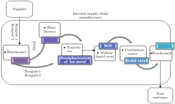
In this paper, we focus on a supply chain of a real steel industry in Canada. The total supply chain consists of eight entities and three echelons (supplier, manufacturer, and customer). Its entities are: supplier, warehouse1, blast furnace, torpedo car, Basic Oxygen Furnace (BOF), continuous caster, warehouse2, and customer, as shown in Figure 1 . The internal supply chain consists of six entities: warehouse1, blast furnace, torpedo car, BOF, continuous caster, and warehouse2. We briefly describe the steel making process in this section.

Figure 1. Supply chain of the steel industry.

3.1. Steel making process in supply chain

Since the end customer requires and orders high quality steel, we categorize steel demand by the degree of sulphur. The higher the degree of sulphur is, the lower the quality of steel. So, for reducing the amount of sulphur, two reagents are used in a steel factory: reagent1 and reagent2. When a customer places an order for steel with low sulphur, it means that the steel needs an especial amount of reagents to achieve the desired degree of sulphur (target sulphur). In such a situation, the amount of reagents is considered as a demand in the supply chain. The demands of the reagents move through the chain from downstream to upstream. The steel factory provides its raw material from the supplier. In this paper, we consider reagent1 and reagent2 as the main materials ordered by the factory. The steel making process is described as follows.

After providing raw materials (reagent1 and reagent2) from a supplier, the material batches are gathered in a warehouse of raw material, which is named warehouse1. Then, in the blast furnace, a batch melting process, which produces batches of molten steel, is implemented. The third step is desulphurization of the hot metal, which is implemented in the torpedo car. In this step, sulphur is removed from the hot metal leaving the blast furnace by injection of two reagents  [40] . After the desulphurization process, the liquid steel is transported to a Basic Oxygen Furnace (BOF). The BOF is a large, open-mouthed, pear-shaped vessel lined with a basic refractory material that refines molten iron from the torpedo car, and ferrous scrap into steel, by injecting a jet of high-purity oxygen to remove carbon as CO and CO₂ . The steel is produced in BOFs and follows similar routes after the molten steel is poured from the furnace. The molten steel is transferred from the ladle metallurgy to the continuous caster, which casts the steel into semi-finished shapes (e.g., slabs, blooms, billets, rounds and other special sections)  [41] .

Since reagents are expensive materials, steel factories are eager to reduce their consumption. An inaccurate prediction of reagents leads to their consummation being more than their demand, especially when the demands of the reagents move through the chain. The bullwhip effect exists in supply chains, which causes demand amplification. So, if it is not controlled, the second echelon manufacturer will order more reagents than the real demands of the customers. This phenomenon causes a lot of cost for the factory. So, in this paper, we focus on demand prediction as one of the main causes of the bullwhip effect. We show that when demands, orders, and lead times are type-2 fuzzy variables, the bullwhip effect is significantly reduced, in comparison with the type-1 fuzzy system.

In order to measure the bullwhip effect, the following process should be developed in the supply chain of a steel industry:

• The end customer’s demand process;
• The policy that the participant at each stage applies to determine its inventory level and order quantity;
• The forecasting method of each stage for predicting demands and orders to the upstream stage  [16] . In order to predict end customer demands, we develop a hybrid expert system. First, we implement an Interval Type-2 FCRM clustering algorithm (IT2 FCRM)  [31] , which was presented in Section  2.1 , for the structure identification phase of the expert system. The outputs of the IT2 FCRM are membership function parameters of antecedents and regression coefficients of consequents in a rule based system.

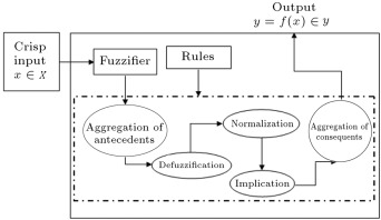
Then, we use the outputs of the IT2 FCRM algorithm in a hybrid expert system. This system is a combination of the Mamdani and Sugeno inference mechanism. It uses regression functions in consequents of the rule base system, similar to the Sugeno method. There is no defuzzification step in the Sugeno system because the consequents are functions. In contrast to the Sugeno method, the antecedents and consequents of the Mamdani rule-based system are fuzzy sets, so defuzzification is required. Therefore, by combining these two inference engines, the new method is obtained. In order to aggregate the antecedents, we use FDNF and FCNF and modify the algorithm proposed by Türksen  [30] . For the implication process, we first defuzzify the result of the aggregated antecedents; then, the result of the defuzzification step is normalized. Next, parameters of the system are tuned with the Adaptive-Network-Based Fuzzy Inference System (ANFIS).

3.2. Steps of the proposed inference system

•  Fuzzification

In this step, in order to identify membership functions and the number of rules, the result of the IT2 FCRM algorithm is used from Section 2.1.  [42] .

•  Aggregation of antecedents

For this step, Türksen’s FDNF and FCNF methods, which are obtained from the truth table, are used in order to aggregate antecedents. The formulations of these methods are presented in Eq. (22) for FDNF. Eq. (23) describes the FCNF method for each upper and lower membership functions. Those two equations are used to aggregate antecedents. Because the consequent parts of our proposed method are auto-regressive moving average functions, FDNF and FCNF are used only for aggregation of antecedents. The implication and aggregation of consequents proposed by Türksen  [30] are not mentioned here. Aggregation of antecedents was presented by Türksen  [30] , and we propose the following stages for the remaining inference engine processes  [42] .

•  Defuzzification

In the Mamdani method, defuzzification is used after inference. However; since FDNF and FCNF are used in our proposed method, aggregated antecedents should be defuzzified in order to take the weighted average of crisp consequents and aggregated antecedents. It means that defuzzification is done in the inference engine. In this paper, Yager defuzzification, which is presented in Eq. (34) , is used. In the following equations, ‘${\textstyle i}$ ’ indicates the number of rules  [42] .

$B_{i}={\frac {\sum _{x}A_{i}(x^{_{\ast }}(r))^{\alpha }\times x}{\sum _{x}x^{\alpha }}}\quad \forall i=1,\ldots ,c0<\alpha <1{\mbox{.}}$

( 34)

•  Normalization

In order to take the weighted average of aggregated antecedents and consequents, the crisp value of each rule obtained from the previous step should be normalized  [42] .

$W_{i}={\frac {B_{i}}{\sum B_{i}}}\quad \forall i=1,\ldots ,c{\mbox{.}}$

( 35)

•  Implication

This step is used in order to weight the crisp consequent of each rule  [42] .

$Y_{i}=W_{i}\times D_{i}\quad \forall i=1,\ldots ,c{\mbox{.}}$

( 36)

•  Aggregation of Consequents

The model output of each rule is aggregated by taking the weighted average of the output of each rule in the fuzzy rule base  [42] .

$Y={\frac {\sum _{i=1:c}Y_{i}}{\sum _{i=1:c}W_{i}}}\quad \forall i=1,\ldots ,c{\mbox{.}}$

( 37)

These steps are used separately for upper and lower membership functions for both FDNF and FCNF. After applying the last step in the inference engine, the final output of the model is obtained by combining the outputs of FDNF and FCNF  [42] . Figure 2 shows the proposed interval type-2 fuzzy hybrid expert system.

Figure 2. Structure of the proposed interval type-2 fuzzy hybrid system.

3.3. The proposed method in a steel supply chain

In order to predict end customer demands, we identify the variables which influence the amount of reagents; Table 1 shows these variables. First, we predict the amount of reagents related to the degree of sulphur with the proposed expert system, in which consequents are regression functions.

Table 1. Input and output variables of a steel company in Canada.

Column	Description
Id	Batch Id column is created by K.I.L
Reagent1	Amount of reagent1 used in the process
Reagent2	Amount of reagent2 used in the process
Startsulphur(ss)	Sulphur level of the batch before the desulphurization process
Endsulphur(es)	Sulphur level of the batch after the desulphurization process
Aimsulphur	The aimed level of sulphur which is planned to be retrieved after desulphurization process
Car	Car identifier. It can be grouped in three categories: small (607–623), medium (637–641 and 601–623), jumbo (630–636)
Pos	Is the specific station in which the sulphurization took place (there are four stations)
KGS	Weight of the batch
Temp	Temperature of the hot metal as it leaves the blast furnace
Practice 1	Indicates a certain type of intervention or modification to the normal operating practice. These take place over the course of desulphurization and are not often known in advance
Practice2
Practice3
Practice4

3.3.1. Predicting the amount of reagent1

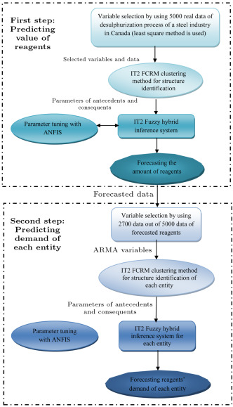
The steps of developing the IT2 fuzzy expert system is depicted in Figure 3 . In the variable selection phase, the following variables are selected: Endsulphur, KGS, Temp, FB, compound1, compound2, compound3, compound4 , and compound5 .

Figure 3. Framework of interval type-2 fuzzy hybrid expert system.

If the starting amount of sulphur in the product is much higher than the expectation, then, two reagents will be added simultaneously. In this case, Reagent2 is the output and Reagent1 is the input of the system. If the starting level of sulphur is close to the targeted value, then only reagent1 will be used  [37] . So, first, we predict the amount of reagent1 and, then, reagent2 is forecasted. In the forecasting process of reagent2, reagent1 is an input of the model.

The first step for forecasting the amount of reagent is to obtain the number of rules and the parameters of antecedents and consequents from the IT2 FCRM clustering algorithm. In the second step, we use the proposed IT2 fuzzy hybrid expert system. In addition, ANFIS is used for tuning the upper and lower membership function parameters of antecedents and regression coefficients in consequents of the IT2F hybrid expert system.

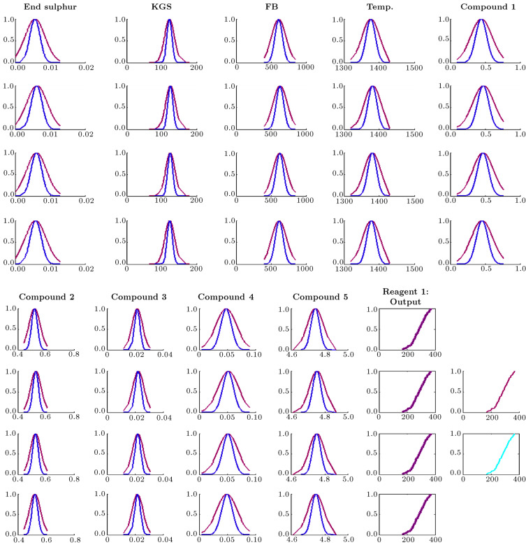
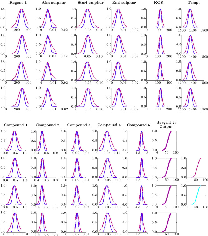
Table A.1 in Appendix A shows the membership function and regression parameters obtained from the IT2 FCRM clustering method. Table A.2 in Appendix A demonstrates the parameters of regression functions in consequents of the IT2F hybrid expert system after tuning. Figure 4 depicts the rule base and inference mechanism for the proposed IT2F hybrid expert system. The first four rows show four rules for the first five variables, and the second four rows depict the four rules for the remaining variables and output of the system. The consequent of each rule is shown in the second column from the right hand side of the last four rows. The last column from the right side of the figure contains two subfigures. The first subfigure from the top indicates the output of the system for both upper and lower bounds. The second subfigure depicts the final output of the system, which is the aggregated result of a combination of FDNF and FCNF.

Table A.1.

Membership function and regression parameters where reagent1 is an output of the IT2 FCRM.

IT2 fuzzy parameters
Rule1
	200.386923889683	199.78273665084	29.154714561463	28.71977903503	0.992306953796287
	${\textstyle {\overline {v}}_{12}}$	${\textstyle {\underline {v}}_{12}}$	${\textstyle {\overline {\sigma }}_{12}}$	${\textstyle {\underline {\sigma }}_{12}}$	${\textstyle a_{2}^{1}}$
	240.378987444701	240.22008138113	6.9997872565227	6.829769919302	0.0680872873954286
	${\textstyle {\overline {v}}_{13}}$	${\textstyle {\underline {v}}_{13}}$	${\textstyle {\overline {\sigma }}_{13}}$	${\textstyle {\underline {\sigma }}_{13}}$	${\textstyle a_{3}^{1}}$
	256.521432108360	256.36670121299	6.2021546606634	6.014976281301	0.0680872873954286
	${\textstyle {\overline {v}}_{14}}$	${\textstyle {\underline {v}}_{14}}$	${\textstyle {\overline {\sigma }}_{14}}$	${\textstyle {\underline {\sigma }}_{14}}$	${\textstyle a_{4}^{1}}$
	270.370177742795	270.19520552506	8.8560714904950	8.792889134618	−0.00164602183212992
	${\textstyle {\overline {v}}_{15}}$	${\textstyle {\underline {v}}_{15}}$	${\textstyle {\overline {\sigma }}_{15}}$	${\textstyle {\underline {\sigma }}_{15}}$	${\textstyle a_{5}^{1}}$
	286.721704150994	286.60505717758	6.3582965563913	6.236712872548	0.0134452820420847
	${\textstyle {\overline {v}}_{16}}$	${\textstyle {\underline {v}}_{16}}$	${\textstyle {\overline {\sigma }}_{16}}$	${\textstyle {\underline {\sigma }}_{16}}$	${\textstyle a_{6}^{1}}$
	301.200089303269	301.08604752786	5.5081435487796	5.369661628348	0.0243054005841259
	${\textstyle {\overline {v}}_{17}}$	${\textstyle {\underline {v}}_{17}}$	${\textstyle {\overline {\sigma }}_{17}}$	${\textstyle {\underline {\sigma }}_{17}}$	${\textstyle a_{7}^{1}}$
	317.277927250643	317.15689587577	5.6781761024962	5.518121102838	−0.0390284665409126
	${\textstyle {\overline {v}}_{18}}$	${\textstyle {\underline {v}}_{18}}$	${\textstyle {\overline {\sigma }}_{18}}$	${\textstyle {\underline {\sigma }}_{18}}$	${\textstyle a_{8}^{1}}$
	334.286405695644	334.12455470885	9.8015632817378	9.656319722936	−0.0160002726338462
	${\textstyle {\overline {v}}_{19}}$	${\textstyle {\underline {v}}_{19}}$	${\textstyle {\overline {\sigma }}_{19}}$	${\textstyle {\underline {\sigma }}_{19}}$	${\textstyle a_{9}^{1}}$
	359.505054161935	359.25061733505	11.076768586337	10.77929424939	0.00266575697423832
					${\textstyle b_{0}^{1}}$
					−6.45425755158067
Rule2	${\textstyle {\overline {v}}_{21}}$	${\textstyle {\underline {v}}_{21}}$	${\textstyle {\overline {\sigma }}_{21}}$	${\textstyle {\underline {\sigma }}_{21}}$	${\textstyle a_{1}^{2}}$
	199.883623589104	200.14662509359	27.733210119964	28.02615271308	0.997597096013124
	${\textstyle {\overline {v}}_{22}}$	${\textstyle {\underline {v}}_{22}}$	${\textstyle {\overline {\sigma }}_{22}}$	${\textstyle {\underline {\sigma }}_{22}}$	${\textstyle a_{2}^{2}}$
	240.356503783117	240.40784233873	6.4835381253128	6.492926097973	−0.0241309895445738
	${\textstyle {\overline {v}}_{23}}$	${\textstyle {\underline {v}}_{23}}$	${\textstyle {\overline {\sigma }}_{23}}$	${\textstyle {\underline {\sigma }}_{23}}$	${\textstyle a_{3}^{2}}$
	256.604227543059	256.67589840588	5.7162738665179	5.689179006228	0.0266908722829839
	${\textstyle {\overline {v}}_{24}}$	${\textstyle {\underline {v}}_{24}}$	${\textstyle {\overline {\sigma }}_{24}}$	${\textstyle {\underline {\sigma }}_{24}}$	${\textstyle a_{4}^{2}}$
	270.126604401960	270.26274128284	8.5418333764863	8.542130177744	−0.0116598585227621
	${\textstyle {\overline {v}}_{25}}$	${\textstyle {\underline {v}}_{25}}$	${\textstyle {\overline {\sigma }}_{25}}$	${\textstyle {\underline {\sigma }}_{25}}$	${\textstyle a_{5}^{2}}$
	286.668763654920	286.73274608976	5.8653181701639	5.915270247358	0.0546987912421173
	${\textstyle {\overline {v}}_{26}}$	${\textstyle {\underline {v}}_{26}}$	${\textstyle {\overline {\sigma }}_{26}}$	${\textstyle {\underline {\sigma }}_{26}}$	${\textstyle a_{6}^{2}}$
	301.163210994670	301.21143581545	5.0292683392491	5.055587995164	−0.00258356434642337
	${\textstyle {\overline {v}}_{27}}$	${\textstyle {\underline {v}}_{27}}$	${\textstyle {\overline {\sigma }}_{27}}$	${\textstyle {\underline {\sigma }}_{27}}$	${\textstyle a_{7}^{2}}$
	317.320595845143	317.35511840629	5.1015789328826	5.113713102915	−0.0160782763996394
	${\textstyle {\overline {v}}_{28}}$	${\textstyle {\underline {v}}_{28}}$	${\textstyle {\overline {\sigma }}_{28}}$	${\textstyle {\underline {\sigma }}_{28}}$	${\textstyle a_{8}^{2}}$
	334.173447366642	334.27992424031	9.2983167439347	9.293036693155	−0.0123426710515560
	${\textstyle {\overline {v}}_{29}}$	${\textstyle {\underline {v}}_{29}}$	${\textstyle {\overline {\sigma }}_{29}}$	${\textstyle {\underline {\sigma }}_{29}}$	${\textstyle a_{9}^{2}}$
	359.472869743826	359.59872066176	10.189734005043	10.20880665460	0.000958262007770827
					${\textstyle b_{0}^{2}}$
					−3.20224236324430
Rule3	${\textstyle {\overline {v}}_{31}}$	${\textstyle {\underline {v}}_{31}}$	${\textstyle {\overline {\sigma }}_{31}}$	${\textstyle {\underline {\sigma }}_{31}}$	${\textstyle a_{1}^{3}}$
	200.084831524207	199.47384345974	28.521312399802	28.61924619775	1.00038021589899
	${\textstyle {\overline {v}}_{32}}$	${\textstyle {\underline {v}}_{32}}$	${\textstyle {\overline {\sigma }}_{32}}$	${\textstyle {\underline {\sigma }}_{32}}$	${\textstyle a_{2}^{3}}$
	240.300442141778	240.13271074641	6.8439544018164	6.858928128989	−0.0187914857187934
	${\textstyle {\overline {v}}_{33}}$	${\textstyle {\underline {v}}_{33}}$	${\textstyle {\overline {\sigma }}_{13}}$	${\textstyle {\underline {\sigma }}_{33}}$	${\textstyle a_{3}^{3}}$
	256.451792214693	256.30035076015	6.1006254784743	6.084011227327	−0.00410993461491671
${\textstyle {\underline {v}}_{34}}$	${\textstyle {\overline {\sigma }}_{34}}$	${\textstyle {\underline {\sigma }}_{34}}$	${\textstyle a_{4}^{3}}$		${\textstyle {\overline {v}}_{34}}$
	270.340229583777	270.12998447347	8.7247474292744	8.759538603582	0.0149190465381253
	${\textstyle {\overline {v}}_{35}}$	${\textstyle {\underline {v}}_{35}}$	${\textstyle {\overline {\sigma }}_{35}}$	${\textstyle {\underline {\sigma }}_{35}}$	${\textstyle a_{5}^{3}}$
	286.692057152096	286.52857224753	6.1929887585724	6.208349034995	−0.0625144882289987
	${\textstyle {\overline {v}}_{36}}$	${\textstyle {\underline {v}}_{36}}$	${\textstyle {\overline {\sigma }}_{36}}$	${\textstyle {\underline {\sigma }}_{36}}$	${\textstyle a_{6}^{3}}$
	301.160692538486	301.02286250282	5.2812794298939	5.302542982667	−0.028968875209102
	${\textstyle {\overline {v}}_{37}}$	${\textstyle {\underline {v}}_{37}}$	${\textstyle {\overline {\sigma }}_{37}}$	${\textstyle {\underline {\sigma }}_{37}}$	${\textstyle a_{7}^{3}}$
	317.260640030407	317.13372907610	5.4389609025414	5.476156928078	0.0337565070894925
	${\textstyle {\overline {v}}_{38}}$	${\textstyle {\underline {v}}_{38}}$	${\textstyle {\overline {\sigma }}_{18}}$	${\textstyle {\underline {\sigma }}_{38}}$	${\textstyle a_{8}^{3}}$
	334.268895045785	334.04485324558	9.6310699934765	9.670662675240	0.0205755915972077
	${\textstyle {\overline {v}}_{39}}$	${\textstyle {\underline {v}}_{39}}$	${\textstyle {\overline {\sigma }}_{39}}$	${\textstyle {\underline {\sigma }}_{39}}$	${\textstyle a_{9}^{3}}$
	359.389624517381	359.14132614800	10.754432441651	10.76161026005	0.0137478195538279
					${\textstyle b_{0}^{3}}$
					5.82769897207618
Rule4
	${\textstyle {\overline {v}}_{41}}$	${\textstyle {\underline {v}}_{41}}$	${\textstyle {\overline {\sigma }}_{41}}$	${\textstyle {\underline {\sigma }}_{41}}$	${\textstyle a_{1}^{4}}$
	200.564962571797	200.19247348018	29.356754189162	29.21609218973	1.00295877840290
	${\textstyle {\overline {v}}_{42}}$	${\textstyle {\underline {v}}_{42}}$	${\textstyle {\overline {\sigma }}_{42}}$	${\textstyle {\underline {\sigma }}_{42}}$	${\textstyle a_{2}^{4}}$
	240.469140900366	240.39103433857	6.9659813293248	6.977026792209	−0.0359335819175612
	${\textstyle {\overline {v}}_{43}}$	${\textstyle {\underline {v}}_{43}}$	${\textstyle {\overline {\sigma }}_{43}}$	${\textstyle {\underline {\sigma }}_{43}}$	${\textstyle a_{3}^{4}}$
	256.627757645573	256.55255206873	6.2040546078353	6.149153117260	0.0258010084103262
	${\textstyle {\overline {v}}_{44}}$	${\textstyle {\underline {v}}_{44}}$	${\textstyle {\overline {\sigma }}_{44}}$	${\textstyle {\underline {\sigma }}_{44}}$	${\textstyle a_{4}^{4}}$
	270.650153530683	270.60291904336	8.8672042415837	8.876849369984	0.0401843806685065
	${\textstyle {\overline {v}}_{45}}$	${\textstyle {\underline {v}}_{45}}$	${\textstyle {\overline {\sigma }}_{45}}$	${\textstyle {\underline {\sigma }}_{45}}$	${\textstyle a_{5}^{4}}$
	286.812715748138	286.76688080765	6.2883402135872	6.312697123053	0.000421580994043325
	${\textstyle {\overline {v}}_{46}}$	${\textstyle {\underline {v}}_{46}}$	${\textstyle {\overline {\sigma }}_{46}}$	${\textstyle {\underline {\sigma }}_{46}}$	${\textstyle a_{6}^{4}}$
	301.264920538835	301.18901571181	5.4216435762859	5.402242700356	−0.0596213198150508
	${\textstyle {\overline {v}}_{47}}$	${\textstyle {\underline {v}}_{47}}$	${\textstyle {\overline {\sigma }}_{47}}$	${\textstyle {\underline {\sigma }}_{47}}$	${\textstyle a_{7}^{4}}$
	317.335079274534	317.24934112582	5.6584438772265	5.621983051787	−0.0363773121353006
	${\textstyle {\overline {v}}_{48}}$	${\textstyle {\underline {v}}_{48}}$	${\textstyle {\overline {\sigma }}_{48}}$	${\textstyle {\underline {\sigma }}_{48}}$	${\textstyle a_{8}^{4}}$
	334.433249345254	334.38228537627	9.8783783207043	9.831625767418	0.0109459600346327
	${\textstyle {\overline {v}}_{49}}$	${\textstyle {\underline {v}}_{49}}$	${\textstyle {\overline {\sigma }}_{49}}$	${\textstyle {\underline {\sigma }}_{49}}$	${\textstyle a_{9}^{4}}$
	359.646364080831	359.47866655465	10.974619178208	10.92916206040	0.00836995833742549
					${\textstyle b_{0}^{4}}$
					13.5331820361316

Table A.2. Parameters of regression functions in consequents for reagent1 after tuning.

Rules	Regression function parameters
Rule1	${\textstyle a_{1}^{1}}$	${\textstyle a_{2}^{1}}$	${\textstyle a_{3}^{1}}$	${\textstyle a_{4}^{1}}$	${\textstyle a_{5}^{1}}$
	16.02	6.611	−50.82	26.23	−27.17
	${\textstyle a_{6}^{1}}$	${\textstyle a_{7}^{1}}$	${\textstyle a_{8}^{1}}$	${\textstyle a_{9}^{1}}$	${\textstyle b_{0}^{1}}$
	43.08	25.6	−59.76	22.47	−9.745
Rule2	${\textstyle a_{1}^{2}}$	${\textstyle a_{2}^{2}}$	${\textstyle a_{3}^{2}}$	${\textstyle a_{4}^{2}}$	${\textstyle a_{5}^{2}}$
	5.87	3.245	−20.63	14.39	2.784
	${\textstyle a_{6}^{2}}$	${\textstyle a_{7}^{2}}$	${\textstyle a_{8}^{2}}$	${\textstyle a_{9}^{2}}$	${\textstyle b_{0}^{2}}$
	10.85	1.444	−22.4	7.383	−10.27
Rule3	${\textstyle a_{1}^{3}}$	${\textstyle a_{2}^{3}}$	${\textstyle a_{3}^{3}}$	${\textstyle a_{4}^{3}}$	${\textstyle a_{5}^{3}}$
	−8.003	2.942	46.46	−42.28	12.88
	${\textstyle a_{6}^{3}}$	${\textstyle a_{7}^{3}}$	${\textstyle a_{8}^{3}}$	${\textstyle a_{9}^{3}}$	${\textstyle b_{0}^{3}}$
	−45.23	−13.58	63.53	−18.02	−9.304
Rule4	${\textstyle a_{1}^{4}}$	${\textstyle a_{2}^{4}}$	${\textstyle a_{3}^{4}}$	${\textstyle a_{4}^{4}}$	${\textstyle a_{5}^{4}}$
	−10.15	−12.41	25.79	1.507	12.34
	${\textstyle a_{6}^{4}}$	${\textstyle a_{7}^{4}}$	${\textstyle a_{8}^{4}}$	${\textstyle a_{9}^{4}}$	${\textstyle b_{0}^{4}}$
	−9.53	−13.72	18.92	−12.33	−10.54

Figure 4. Rule base and inference mechanism in which reagent1 is an output for the proposed IT2F hybrid expert system.

3.3.2. Predicting end customer demand with ARMA method

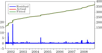
The first step for measuring the bullwhip effect is to predict end customer demand. After predicting the amount of reagent1, the end customer demand should be predicted for steel with different degrees of sulphur in the desulphurization process for the next 300 days. An Auto Regressive Moving Average (ARMA) method is used for demand prediction. It means that the consequent parts of the IT2F hybrid expert system are ARMA functions. 2700 data from 5000 data of the predicted amount of reagents are selected for identifying the ARMA function. After applying the statistical test, these variables are selected: AR(2), AR(4), AR(5), AR(9), MA(1), MA(2), MA(3), MA(4), and MA(80). Table 2 shows the results of the statistical test. Figure 5 depicts the residual of the model and actual output, as well as the fitted output.

Table 2. Coefficient test for reagent1.

Variables	Coefficient	Std. error	${\textstyle t}$ -statistic	Prob.
AR(2)	−0.103309	0.004282	−24.12827	0.0000
AR(4)	0.824410	0.006266	131.5599	0.0000
AR(5)	0.357875	0.017997	19.88511	0.0000
AR(9)	−0.077964	0.018936	−4.117280	0.0000
MA(1)	0.980674	0.018719	52.38938	0.0000
MA(2)	1.075049	0.016387	65.60504	0.0000
MA(3)	1.094153	0.016185	67.60324	0.0000
MA(4)	0.249138	0.019124	13.02720	0.0000
MA(80)	0.018188	0.004884	3.724168	0.0002
${\textstyle R}$ -squared	0.999889	Mean dependent var	285.4900	${\textstyle R}$ -squared
Adjusted ${\textstyle R}$ -squared	0.999888	S.D. dependent var	46.92681	Adjusted ${\textstyle R}$ -squared
S.E. of regression	0.495660	Akaike info criterion	1.437487	S.E. of regression
Sum squared resid	658.9117	Schwarz criterion	1.457212	Sum squared resid
Log likelihood	−1925.139	Hannan–Quinn criter.	1.444622	Log likelihood

Figure 5. Actual and fitted data with the residual of the system.

After determining ARMA variables, we divide 2700 data of reagents into nine groups for nine ARMA variables, which were selected from the variable selection phase. This leads to allocating 300 data to each variable for predicting end customer demand for the next 300 days. Figure 3 depicts the results of applying the IT2 FCRM method using 300 data for each ARMA variable.

In the next step, ANFIS is used for tuning the upper and lower membership function parameters of antecedents and ARMA coefficients in the consequents of the IT2F hybrid expert system. Table A.2 in Appendix A demonstrates the parameters of regression functions in consequents after tuning. In this table, ${\textstyle {\overline {v}}_{jk}}$ is the mean of the upper Gaussian membership function and ${\textstyle {\underline {v}}_{jk}}$ is the mean of the lower Gaussian membership function. In addition, ${\textstyle {\overline {\sigma }}_{jk}}$ and ${\textstyle {\underline {\sigma }}_{jk}}$ are the standard deviations of upper and lower Gaussian membership functions, respectively. In Appendix A , Table A.3 shows the tuned parameters of upper membership functions, and Table A.4 shows the tuned parameters of lower membership functions.

Table A.3. Parameters of upper membership function for reagent1 after tuning.

Rules	Membership functions parameters
Rule1	${\textstyle [{\overline {v}}_{11},{\overline {\sigma }}_{11}]}$	${\textstyle [{\overline {v}}_{12},{\overline {\sigma }}_{12}]}$	${\textstyle [{\overline {v}}_{13},{\overline {\sigma }}_{13}]}$	${\textstyle [{\overline {v}}_{14},{\overline {\sigma }}_{14}]}$	${\textstyle [{\overline {v}}_{15},{\overline {\sigma }}_{15}]}$
	[29.15 200.4]	[7.007 240.4]	[6.18 256.5]	[8.865 270.4]	[6.422 286.7]
	${\textstyle [{\overline {v}}_{16},{\overline {\sigma }}_{16}]}$	${\textstyle [{\overline {v}}_{17},{\overline {\sigma }}_{17}]}$	${\textstyle [{\overline {v}}_{18},{\overline {\sigma }}_{18}]}$	${\textstyle [{\overline {v}}_{19},{\overline {\sigma }}_{19}]}$
	[5.454 301.2]	[5.632 317.3]	[9.82 334.3]	[11.09 359.5]
Rule2	${\textstyle [{\overline {v}}_{21},{\overline {\sigma }}_{21}]}$	${\textstyle [{\overline {v}}_{22},{\overline {\sigma }}_{22}]}$	${\textstyle [{\overline {v}}_{23},{\overline {\sigma }}_{23}]}$	${\textstyle [{\overline {v}}_{24},{\overline {\sigma }}_{24}]}$	${\textstyle [{\overline {v}}_{25},{\overline {\sigma }}_{25}]}$
	[27.73 199.9]	[6.491 240.4]	[5.71 256.6]	[8.555 270.1]	[5.895 286.7]
	${\textstyle [{\overline {v}}_{26},{\overline {\sigma }}_{26}]}$	${\textstyle [{\overline {v}}_{27},{\overline {\sigma }}_{27}]}$	${\textstyle [{\overline {v}}_{28},{\overline {\sigma }}_{28}]}$	${\textstyle [{\overline {v}}_{29},{\overline {\sigma }}_{29}]}$
	[4.998 301.2]	[5.089 317.3]	[9.3 334.2]	[10.2 359.5]
Rule3	${\textstyle [{\overline {v}}_{31},{\overline {\sigma }}_{31}]}$	${\textstyle [{\overline {v}}_{32},{\overline {\sigma }}_{32}]}$	${\textstyle [{\overline {v}}_{33},{\overline {\sigma }}_{33}]}$	${\textstyle [{\overline {v}}_{34},{\overline {\sigma }}_{34}]}$	${\textstyle [{\overline {v}}_{35},{\overline {\sigma }}_{35}]}$
	[28.52 200.1]	[6.836 240.3]	[6.125 256.5]	[8.7 270.3]	[6.133 286.7]
	${\textstyle [{\overline {v}}_{36},{\overline {\sigma }}_{36}]}$	${\textstyle [{\overline {v}}_{37},{\overline {\sigma }}_{37}]}$	${\textstyle [{\overline {v}}_{38},{\overline {\sigma }}_{38}]}$	${\textstyle [{\overline {v}}_{39},{\overline {\sigma }}_{39}]}$
	[5.331 301.2]	[5.469 317.3]	[9.626 334.3]	[10.75 359.4]
Rule4	${\textstyle [{\overline {v}}_{41},{\overline {\sigma }}_{41}]}$	${\textstyle [{\overline {v}}_{42},{\overline {\sigma }}_{42}]}$	${\textstyle [{\overline {v}}_{43},{\overline {\sigma }}_{43}]}$	${\textstyle [{\overline {v}}_{44},{\overline {\sigma }}_{44}]}$	${\textstyle [{\overline {v}}_{45},{\overline {\sigma }}_{45}]}$
	[29.35 200.6]	[6.96 240.5]	[6.207 256.6]	[8.872 270.7]	[6.253 286.8]
	${\textstyle [{\overline {v}}_{46},{\overline {\sigma }}_{46}]}$	${\textstyle [{\overline {v}}_{47},{\overline {\sigma }}_{47}]}$	${\textstyle [{\overline {v}}_{48},{\overline {\sigma }}_{48}]}$	${\textstyle [{\overline {v}}_{49},{\overline {\sigma }}_{49}]}$
	[5.456 301.3]	[5.686 317.3]	[9.864 334.4]	[10.95 359.6]

Table A.4. Parameters of lower membership function for reagent1 after tuning.

Rules	Membership functions parameters
Rule1	${\textstyle [{\underline {v}}_{11},{\underline {\sigma }}_{11}]}$	${\textstyle [{\underline {v}}_{12},{\underline {\sigma }}_{12}]}$	${\textstyle [{\underline {v}}_{13},{\underline {\sigma }}_{13}]}$	${\textstyle [{\underline {v}}_{14},{\underline {\sigma }}_{14}]}$	${\textstyle [{\underline {v}}_{15},{\underline {\sigma }}_{15}]}$
	[28.72 199.8]	[6.829 240.2]	[6.015 256.4]	[8.791 270.2]	[6.235 286.6]
	${\textstyle [{\underline {v}}_{16},{\underline {\sigma }}_{16}]}$	${\textstyle [{\underline {v}}_{17},{\underline {\sigma }}_{17}]}$	${\textstyle [{\underline {v}}_{18},{\underline {\sigma }}_{18}]}$	${\textstyle [{\underline {v}}_{19},{\underline {\sigma }}_{19}]}$
	[5.368 301.1]	[5.516 317.2]	[9.657 334.1]	[10.78 359.3]
Rule2	${\textstyle [{\underline {v}}_{21},{\underline {\sigma }}_{21}]}$	${\textstyle [{\underline {v}}_{22},{\underline {\sigma }}_{22}]}$	${\textstyle [{\underline {v}}_{23},{\underline {\sigma }}_{23}]}$	${\textstyle [{\underline {v}}_{24},{\underline {\sigma }}_{24}]}$	${\textstyle [{\underline {v}}_{25},{\underline {\sigma }}_{25}]}$
	[28.03 200.1]	[6.493 240.4]	[5.689 256.7]	[8.861 270.3]	[5.915 286.7]
	${\textstyle [{\underline {v}}_{26},{\underline {\sigma }}_{26}]}$	${\textstyle [{\underline {v}}_{27},{\underline {\sigma }}_{27}]}$	${\textstyle [{\underline {v}}_{28},{\underline {\sigma }}_{28}]}$	${\textstyle [{\underline {v}}_{29},{\underline {\sigma }}_{29}]}$
	[5.054 301.2]	[5.111 317.4]	[9.293 334.3]	[10.21 359.6]
Rule3	${\textstyle [{\underline {v}}_{31},{\underline {\sigma }}_{31}]}$	${\textstyle [{\underline {v}}_{32},{\underline {\sigma }}_{32}]}$	${\textstyle [{\underline {v}}_{33},{\underline {\sigma }}_{33}]}$	${\textstyle [{\underline {v}}_{34},{\underline {\sigma }}_{34}]}$	${\textstyle [{\underline {v}}_{35},{\underline {\sigma }}_{35}]}$
	[28.62 199.5]	[6.859 240.1]	[6.084 256.3]	[8.761 270.1]	[6.211 286.5]
	${\textstyle [{\underline {v}}_{36},{\underline {\sigma }}_{36}]}$	${\textstyle [{\underline {v}}_{37},{\underline {\sigma }}_{37}]}$	${\textstyle [{\underline {v}}_{38},{\underline {\sigma }}_{38}]}$	${\textstyle [{\underline {v}}_{39},{\underline {\sigma }}_{39}]}$
	[5.305 301]	[5.48 317.1]	[9.67 334]	[10.76 359.1]
Rule4	${\textstyle [{\underline {v}}_{41},{\underline {\sigma }}_{41}]}$	${\textstyle [{\underline {v}}_{42},{\underline {\sigma }}_{42}]}$	${\textstyle [{\underline {v}}_{43},{\underline {\sigma }}_{43}]}$	${\textstyle [{\underline {v}}_{44},{\underline {\sigma }}_{44}]}$	${\textstyle [{\underline {v}}_{45},{\underline {\sigma }}_{45}]}$
	[29.22 200.2]	[6.977 240.4]	[6.149 256.6]	[8.877 270.6]	[6.312 286.8]
	${\textstyle [{\underline {v}}_{46},{\underline {\sigma }}_{46}]}$	${\textstyle [{\underline {v}}_{47},{\underline {\sigma }}_{47}]}$	${\textstyle [{\underline {v}}_{48},{\underline {\sigma }}_{48}]}$	${\textstyle [{\underline {v}}_{49},{\underline {\sigma }}_{49}]}$
	[5.403 301.2]	[5.623 317.2]	[9.831 334.4]	[10.93 359.5]

After identifying the parameters of the system with IT2 FCRM, the inference step should be performed. Eq. (38) shows the structure of the rules, which are used in the IT2F hybrid expert system for the inference phase. We assign nine linguistic terms to the ARMA variables: “very very high”, “very high”, “high”, “medium high”, “medium”, “medium low”, “low”, “very low”, and “very very low”. This means that the demand for each reagent is related to the amount of sulphur. For example, when the amount of sulphur is “very very low” it consumes lower reagents, and the demand for low sulphur steel is “very very high”. Also, the demand for “very low” sulphur steel is “very high”. The next linguistic is “low” sulphur, which is equal to “high” demand. “medium low” sulphur has “medium high” demand. Other linguistic variables are assigned to IT2 fuzzy demands by the same order. This order continues to reach the final linguistic, which is “very very high” sulphur, whose demand is “very very low”:

${\begin{array}{l}\displaystyle R^{k}:{\mbox{IF  }}D_{t-2}^{k}{\mbox{  is  }}{\tilde {A}}{\mbox{  AND  }}D_{t-4}^{k}{\mbox{  is  }}{\tilde {B}}{\mbox{  AND  }}D_{t-5}^{k}{\mbox{  is  }}{\tilde {C}}{\mbox{AND  }}D_{t-9}^{k}{\mbox{  is  }}{\tilde {E}}{\mbox{  AND  }}\epsilon _{t-1}{\mbox{  is  }}{\tilde {F}}{\mbox{  AND  }}\epsilon _{t-2}{\mbox{  is  }}{\tilde {G}}{\mbox{  AND  }}\epsilon _{t-3}{\mbox{is  }}{\tilde {H}}{\mbox{  AND  }}\epsilon _{t-4}{\mbox{  is  }}{\tilde {I}}{\mbox{  AND  }}\epsilon _{t-80}{\mbox{  is  }}{\tilde {J}}{\mbox{  THEN  }}D_{t}^{k}=\\\displaystyle =\varphi _{1}\times D_{t-2}^{k}+\varphi _{2}\times D_{t-4}^{k}+\varphi _{3}\times D_{t-5}^{k}+\varphi _{4}\times D_{t-9}^{k}+\\\displaystyle +\theta _{1}\times \epsilon _{t-1}^{k}+\theta _{2}\times \epsilon _{t-2}^{k}+\theta _{3}\times \epsilon _{t-3}^{k}+\theta _{4}\times \epsilon _{t-4}^{k}+\\\displaystyle +\theta _{5}\times \epsilon _{t-80}^{k}{\mbox{,}}\end{array}}$

( 38)

where ${\textstyle R^{k}}$ is the ${\textstyle k}$ th rule, and ${\textstyle {\tilde {A}},{\tilde {B}},{\tilde {C}},{\tilde {E}},{\tilde {F}},{\tilde {G}},{\tilde {H}},{\tilde {I}}}$ , and ${\textstyle {\tilde {J}}}$ are type-2 linguistic variables. In Eq. (38) , ${\textstyle D_{t-i}^{k}}$ indicates the demand for the ${\textstyle (t-i)}$ th period and the ${\textstyle k}$ th rule; ${\textstyle \varphi _{i}}$ is the autoregressive coefficient. In Eq. (38) , ${\textstyle \epsilon _{t-j}^{k}}$ indicates the moving average for the ${\textstyle (t-j)}$ th period and the ${\textstyle k}$ th rule; ${\textstyle \theta _{i}}$ is the moving average coefficient, where, ${\textstyle i=2,4,5,9}$ and ${\textstyle j=1,2,3,4,80}$ .

Using the IT2F hybrid expert system with the above rule base, which consists of four rules, we forecast end customer demand.

3.3.3. Predicting the order policy for each entity in the chain

The second step for measuring the bullwhip effect is the policy that each participant at each stage applies to determine its inventory level and order quantity. The order that moves from end customer to upstream (warehouse2) is calculated with the following equations  [43] (we extend the type-1 fuzzy ordering policy presented by  [43] to the type-2 fuzzy model):

${\tilde {S}}_{k,t}={\tilde {m}}_{k,t}+z_{k}{\sqrt {v_{k,t}}}{\mbox{,}}$

( 39)

where:

${\tilde {m}}_{k,t}=E(\sum _{i=1}^{{\tilde {l}}_{k+1}}{\tilde {D}}_{k,t+i}\vert {\tilde {D}}_{k,t}){\mbox{,}}$

( 40)

where ${\textstyle {\tilde {S}}_{k,t}}$ is an interval type-2 fuzzy value of “the order-up-to level” at stage ${\textstyle k}$ and period ${\textstyle t}$ , ${\textstyle E(\sum _{i=1}^{{\tilde {l}}_{k+1}}{\tilde {D}}_{k,t+i}\vert {\tilde {D}}_{k,t})}$ is the mean of the interval type-2 fuzzy set, and ${\textstyle var(\sum _{i=1}^{{\tilde {l}}_{k+1}}{\tilde {D}}_{k,t+i}\vert {\tilde {D}}_{k,t})}$ is equal to the variance of interval type-2 fuzzy sets. In order to calculate the mean and variance of interval type-2 fuzzy sets, we use Wu and Mendel’s definitions  [44] .

Definition 1.

Centroid of an IT2 FS. The centroid ${\textstyle C_{\tilde {A}}}$ of an IT2 FS ${\textstyle {\tilde {A}}}$ is the union of the centroids of all its embedded T1 FSs ${\textstyle A_{e}}$ , i.e.  [44] :

$C_{\tilde {A}}\equiv {\underset {\forall A_{e}}{\bigcup }}C(A_{e})=[C_{l}({\tilde {A}}),C_{r}({\tilde {A}})]{\mbox{,}}$

( 43)

where ${\textstyle \cup }$ is the union operation, and:

$C_{l}({\tilde {A}})={\underset {\forall A_{e}}{min}}C(A_{e}){\mbox{,}}$

( 44)

${\textstyle C_{l}({\tilde {A}})}$ and ${\textstyle C_{r}({\tilde {A}})}$ can be expressed as  [44] , [45] , [46]  and [47] :

$C_{l}({\tilde {A}})={\frac {\sum _{i=1}^{L}x_{i}{\overline {\mu }}_{\tilde {A}}(x_{i})+\sum _{i=L+1}^{N}x_{i}{\underline {\mu }}_{\tilde {A}}(x_{i})}{\sum _{i=1}^{L}{\overline {\mu }}_{\tilde {A}}(x_{i})+\sum _{i=L+1}^{N}{\underline {\mu }}_{\tilde {A}}(x_{i})}}$

( 46)

where ${\textstyle {\underline {\mu }}_{\tilde {A}}(x_{i})}$ is the lower membership function, and ${\textstyle {\overline {\mu }}_{\tilde {A}}(x_{i})}$ is the upper one in domain ${\textstyle x_{i}}$ .

Definition 2.

Variance of an IT2 FS. One way to define variance ${\textstyle V_{\tilde {A}}}$ of an IT2 FS ${\textstyle {\tilde {A}}}$ is to find the union of the variances of all its embedded T1 FSs ${\textstyle A_{e}}$ , i.e.  [44] :

$V_{\tilde {A}}={\underset {\forall A_{e}}{\bigcup }}v(A_{e})={\underset {\forall A_{e}}{\bigcup }}[{\frac {\sum _{i=1}^{N}[x_{i}-C(A_{e})]^{2}\mu _{A_{e}}(x_{i})}{\sum _{i=1}^{N}\mu _{A_{e}}(x_{i})}}]{\mbox{.}}$

( 48)

Since there are an uncountable number of ${\textstyle A_{e}}$ , this method cannot compute the variances of all ${\textstyle A_{e}}$ ; Wu and Mendel  [44] have presented Eqs.  and  to calculate the variance of IT2F sets:

$v_{\tilde {A}}(A_{e})={\frac {\sum _{i=1}^{N}[x_{i}-C(A)]^{2}\mu _{A_{e}}(x_{i})}{\sum _{i=1}^{N}\mu _{A_{e}}(x_{i})}}{\mbox{,}}$

( 49)

where ${\textstyle C(A)}$ is the center of the centroid of ${\textstyle {\tilde {A}}}$ and ${\textstyle C_{\tilde {A}}}$ that was given in Eq. (43)   [44] .

3.3.4. Demand prediction of each entity in the supply chain

The third step that should be determined for measuring the bullwhip effect is the demand forecasting method of each entity  [16]  and [43] . It is assumed that each entity in the supply chain has the same inventory and order policy as follows  [16] :

${\tilde {D}}_{k+1,t}={\tilde {D}}_{k,t}+({\tilde {S}}_{k,t}-{\tilde {S}}_{k,t-1}){\mbox{,}}$

( 51)

where ${\textstyle {\tilde {S}}_{k,t}}$ is an interval type-2 fuzzy value of “the order-up-to level” at stage ${\textstyle k}$ and period ${\textstyle t}$ , and ${\textstyle {\tilde {D}}_{k,t}}$ is an interval type-2 fuzzy value of “demand” at stage ${\textstyle k}$ and period ${\textstyle t}$ . In order to predict the demand of each entity in supply chains, we use the proposed interval type-2 fuzzy hybrid expert system. First, we use the IT2 FCRM algorithm to cluster the data of these variables: ${\textstyle ({\tilde {D}}_{k+1,t},{\tilde {D}}_{k,t},{\tilde {S}}_{k,t},{\tilde {S}}_{k,t-1})}$ . Then, the following rule base system is utilized in an interval type-2 fuzzy hybrid expert system for the inference phase. It should be mentioned that ANFIS is implemented seven times for tuning the parameters of the system for each entity in the supply chain:

${\begin{array}{l}\displaystyle R^{k}:{\mbox{IF  }}{\tilde {D}}_{k,t}{\mbox{  is  }}{\tilde {A}}{\mbox{  AND  }}{\tilde {S}}_{k,t}{\mbox{  is  }}{\tilde {B}}{\mbox{  AND  }}{\tilde {S}}_{k,t-1}{\mbox{  is  }}{\tilde {C}}{\mbox{,}}\quad {\mbox{THEN  }}{\tilde {D}}_{k+1,t}=\gamma \times {\tilde {D}}_{k,t}+(\delta \times {\tilde {S}}_{k,t}-\\\displaystyle -\tau \times {\tilde {S}}_{k,t-1})\end{array}}$

( 52)

where ${\textstyle \gamma ,\delta }$ and ${\textstyle \tau }$ are regression coefficients. We consider Eq. (51) , the ordering policy, as the regression function for predicting the value of ${\textstyle {\tilde {D}}_{k+1,t}}$ .

3.3.5. Measuring and reducing bullwhip effect in type-1 and type-2 fuzzy environment

In order to measure the bullwhip effect in the type-1 fuzzy environment, the amount of reagents should be predicted. We use the type-1 fuzzy expert system for predicting the amount of reagents. The first phase of the type-1 fuzzy expert system is structure identification with type-1 fuzzy ${\textstyle c}$ -regression clustering  [29] . This algorithm has been presented by Li et al.  [29] , and we use it with some modifications.

The first modification is the use of a Gaussian mixture for generating the partition matrix. The other modification is to use the weighted least square method, presented in Eq. (2) , for producing regression coefficients instead of Eq. (57) .

In FCRM, the distance between the data pair and the cluster representative is defined by Eq. (53) . The goal of the FCRM algorithm is to minimize the objective function, represented in Eq. (54) . Eq. (56) shows the constraint in the FCRM algorithm, wherein the summation of memberships of a data point in all clusters has to be one  [29] :

$d_{ik}(\theta _{i})=\vert y_{k}-[x_{k}1]\cdot \theta _{i}^{T}\vert {\mbox{.}}$

( 53)

where ${\textstyle {\overset {\mbox{ˆ}}{x}}_{k}=[x_{k},1],m\in (1,\infty )}$ is the fuzzy weighting exponent, and ${\textstyle \mu _{ik}\in [0,1]}$ is the fuzzy membership degree of the ${\textstyle k}$ th data pair belonging to the ${\textstyle i}$ th cluster. Eq. (55) shows this membership function:

$\mu _{ik}={\frac {1}{\sum _{j=1}^{c}[d_{ik}(\theta _{i})/d_{jk}(\theta _{j})]^{2/(m-1)}}}{\mbox{,}}$

( 55)

Eqs.  and  show the means and standard deviations of the Gaussian membership function of premises  [29]  and [39] :

$v_{ij}={\frac {\sum _{k=1}^{n}\mu _{ik}x_{kj}}{\sum _{k=1}^{n}\mu _{ik}}}{\mbox{,}}\quad i=1,2,\ldots ,cj=1,2,\ldots ,M{\mbox{,}}$

( 58)

The consequent parameters are defined by Eq. (60)   [29]  and [39] :

${\begin{array}{l}\displaystyle y=p\theta +e{\mbox{,}}\quad \theta =[\theta _{1}^{0},\ldots ,\theta _{1}^{M},\ldots ,\theta _{c}^{0},\ldots ,\theta _{c}^{M}]{\mbox{,}}\quad y=[y_{1},y_{2},\ldots \\\displaystyle y_{n}]{\mbox{,}}\end{array}}$

( 60)

where ${\textstyle e=[e_{1},e_{2},\ldots ,e_{n}]^{T}}$ is the error vector, ${\textstyle e_{k}=y_{k}-{\overset {\mbox{ˆ}}{y}}_{k}(1\leq k\leq n)}$ ,

${\begin{array}{l}\displaystyle p^{i}(x_{k})=[1,\lambda _{1k}x_{k1},\ldots ,\lambda _{1k}x_{kM},\ldots ,1,\lambda _{ck}x_{k1},\ldots \\\displaystyle \lambda _{ck}x_{kM}]{\mbox{,}}\end{array}}$

( 61)

where ${\textstyle x_{kj}(1\leq k\leq n,1\leq j\leq d)}$ is the ${\textstyle j}$ th element of the ${\textstyle k}$ th input and ${\textstyle \lambda _{ik}(1\leq i\leq c,1\leq k\leq n)}$ is the combination of weights of rules  [29]  and [39] .

$\lambda _{ik}={\frac {w_{i}}{\sum _{i=1}^{n}w_{i}}}{\mbox{.}}$

( 62)

After identifying the parameters of antecedents and consequents, the type-1 fuzzy expert system is used for predicting the amount of reagents. Then, the end customer demand is predicted for steel with different degrees of sulphur in the desulphurization process for the next 300 days. The Auto Regressive Moving Average (ARMA) method is used for demand prediction. It means that the consequent parts of the type-1 fuzzy expert system are ARMA functions.

The next step for measuring the bullwhip effect is the policy that each participant at each stage applies to determine its inventory level and order quantity. The order that moves from end customer to upstream (warehouse2) is calculated with the method presented in  [43] . We explained that method in Section  3.3.3 for the type-2 fuzzy system. In this section, we use it in a type-1 fuzzy expert system.

After predicting end customer demand, determining ordering policy, and predicting the demands of each entity in the supply chain, the bullwhip effect is measured with both a type-1 fuzzy expert system and an interval type-2 fuzzy hybrid expert system.

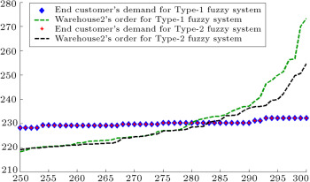
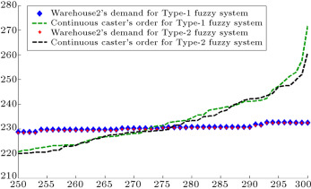
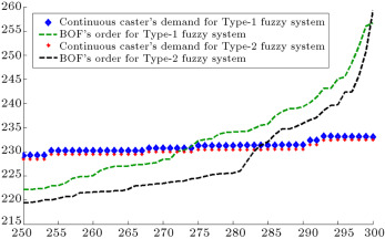
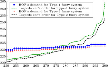
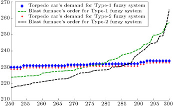
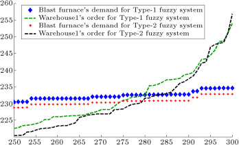
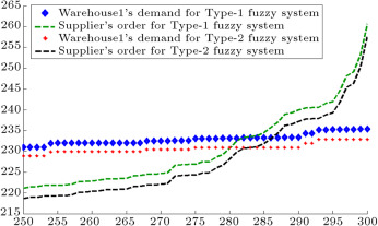
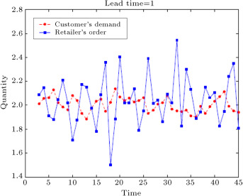
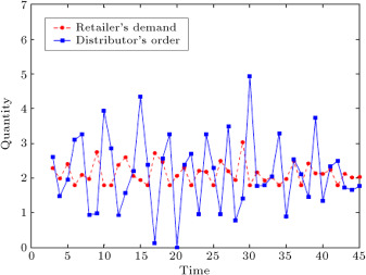
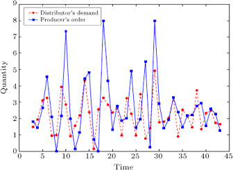
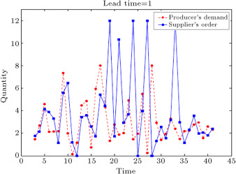
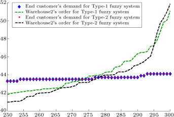
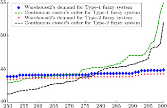
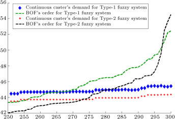
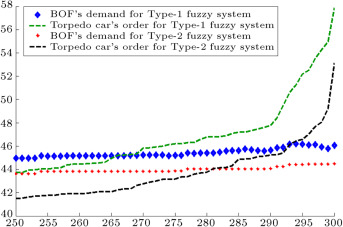
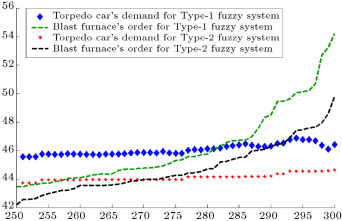
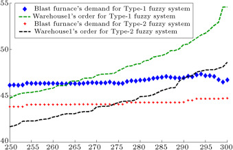
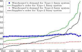
When demands move from downstream to upstream, they are amplified. This demand amplification is named the bullwhip effect. Figure 6 , Figure 7 , Figure 8 , Figure 9 , Figure 10 , Figure 11  and Figure 12 depict the demand and order of each entity for type-1 and interval type-2 fuzzy systems, as well as demand amplification (bullwhip effect), in the supply chain. In order to show demand amplification clearly in these figures, we use the last 51 data points from 300 data. If we used the whole 300 data, the boundary of lines would not be recognizable because of the massive data points in the figures. As these figures show, the bullwhip effect is significantly reduced by our proposed interval type-2 fuzzy hybrid expert system in comparison with the type-1 fuzzy expert system and fuzzy time series presented in  [16] .

Figure 6. End customer’s demand and warehouse2’s order (first entity in manufacturer tier).

Figure 7. Warehouse2’s demand and continuous caster’s order (second entity in manufacturer tier).

Figure 8. Continuous caster’s demand and BOF’s order (third entity in manufacturer tier).

Figure 9. BOF’s demand and torpedo car’s order (forth entity in manufacturer tier).

Figure 10. Torpedo car’s demand and blast furnace order (fifth entity in manufacturer tier).

Figure 11. Blast furnace demand and warehouse1’s order (sixth entity in manufacturer tier).

Figure 12. Warehouse1’s demand and supplier’s order.

In order to validate our model, we compare the results of the interval type-2 fuzzy hybrid expert system with the type-1 fuzzy time series method in the literature. This method has been presented by Fazel Zarandi et al.  [16] . They used the fuzzy time series for demand prediction. The method that they applied for predicting end customer demand was a fuzzy triangular number, in which the midpoint was ARMA and the left and right points were generated randomly. Figure 13 , Figure 14 , Figure 15  and Figure 16 show the results of the demand and order prediction of that model. As Figure 13 , Figure 14 , Figure 15  and Figure 16 show, the variability of demands and orders from downstream to upstream is high in comparison with our proposed method.

Figure 13. Customer’s demand and retailer’s order forecasted by type-1 fuzzy time series  [16] .

Figure 14. Retailer’s demand and distributer’s order forecasted by type-1 fuzzy time series  [16] .

Figure 15. Distributer’s demand and producer’s order forecasted by type-1 fuzzy time series  [16] .

Figure 16. Producer’s demand and supplier’s order forecasted by type-1 fuzzy time series  [16] .

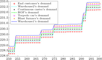
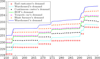
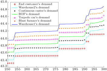
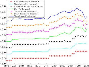
Figure 17 depicts demands of the end customer, warehouse2, continuous caster, BOF, torpedo car, blast furnace, and warehouse1, which are obtained from the interval type-2 fuzzy hybrid expert system. In order to show demand amplification clearly in Figure 17  and Figure 18 , we use the last 51 data points from 300 data. Figure 17 shows that the difference between the demands of each entity and the demands of its upstream supplier is very low. Figure 18 depicts the demands of the entities forecast by the type-1 fuzzy expert system. This figure shows that the difference between the demands of each entity and the demands of its upstream supplier is higher than our proposed interval type-2 fuzzy hybrid expert system. It means that the demand variation in the type-1 fuzzy expert system is more than the demand amplification in our proposed interval type-2 fuzzy hybrid expert system.

Figure 17. Demands of each entity in the chain forecasted by IT2F hybrid expert system.

Figure 18. Demands of each entity in the chain forecasted by type-1 fuzzy expert system.

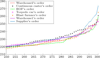
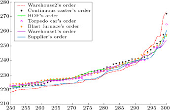
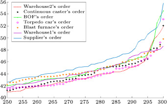
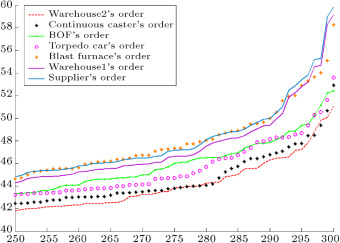
Figure 19 depicts the orders of warehouse2, continuous caster, BOF, torpedo car, blast furnace, warehouse1, and supplier. The orders of each entity are very close to its upstream cooperator in the chain. Figure 20 shows the orders of each entity calculated with the type-1 fuzzy expert system. In comparison with the IT2F system, the orders of each entity are farther from its upstream cooperator in the chain.

Figure 19. Orders of each entity in the chain forecasted by IT2F hybrid expert system.

Figure 20.

Orders of each entity in the chain forecasted by type-1 fuzzy expert system.

If  ${\textstyle V\,ar(D_{end~customer})<V\,ar(D_{Warehouse2})<V\,ar(D_{Continuous~caster})<V\,ar(D_{BOF})<V\,ar(D_{Torpedo~car})<V\,ar(D_{Blast~Furnace})<V\,ar(D_{Warehouse1})}$ exists between the demand variance of end customer, warehouse2, continuous caster, BOF, torpedo car, blast furnace, and warehouse1, it means that the bullwhip effect exists in the chain. Table 3 shows that in the type-1 fuzzy method, the above relation between the variance of demands is true. However, in the proposed interval type-2 fuzzy hybrid expert system, the inequality sign (“ >”) exists between the variance of each entity from downstream (“end customer”) to upstream (“warehouse1”). It means that the bullwhip effect in the steel supply chain is significantly reduced with the proposed IT2F hybrid expert system.

Table 3. Value of demand variance and BW metric of reagent1 for different entities.

	End customer	Warehouse2	Continuous caster	BOF	Torpedo car	Blast furnace	Warehouse1
Type-1 fuzzy variance of demands	400.8059594	401.0527292	402.2934512	404.1183751	404.4611015	405.5177001	406.6546425
Metric value for Type-1 expert system	–	0.000615684	0.003093663	0.0045363	0.000848084	0.002612361	0.002803681
Interval Type-2 fuzzy variance of demands	408.3135523	408.1530656	407.9833725	407.8328927	407.5073497	407.2617169	407.1679306
Metric value for IT2F hybrid expert system	–	0.000393048	0.000415758	0.000368838	0.000798226	0.000602769	0.000230285

In order to quantify the bullwhip effect, we utilize a metric proposed by Li et al.  [48] . This metric uses the variance of demands predicted by our proposed interval type-2 fuzzy hybrid expert system. Then, we calculate this metric with the variance of demands predicted by the type-1 fuzzy expert system and the method proposed by Fazel Zarandi et al.  [16] . In the next step, we compare the results of the metric obtained from those aforementioned methods. Eq. (63) shows this metric:

$A_{i,j}={\frac {V\,ar(D_{i})-V\,ar(D_{j})}{V\,ar(D_{j})}}{\mbox{.}}$

( 63)

When this metric is used, if ${\textstyle \vert A_{k+2,k+1}\vert >\vert A_{k+1,k}\vert }$ , it is said that the information transformation propagates from stage ${\textstyle k}$ to ${\textstyle k+2}$ in an increasing magnitude. Otherwise, if ${\textstyle \vert A_{k+2,k+1}\vert <\vert A_{k+1,k}\vert }$ , we say that the information transformation propagates from stage ${\textstyle k}$ to ${\textstyle k+2}$ in a decreasing magnitude  [16] . In order to calculate interval type-2 fuzzy variance, Wu and Mendel’s formulation  [44] , presented in Section  3.3.3 , is used. The results of computing the metric value are presented in Table 3 . The results show that the metric value for our proposed interval type-2 fuzzy hybrid expert system is reduced significantly in comparison with the type-1 fuzzy system. After comparing the results of the proposed method (Table 3 ) with the results of Fazel Zarandi et al.  [16] , which are shown in Table 4 , this conclusion is obtained: The metric value for each entity is reduced drastically in the interval type-2 fuzzy hybrid expert system in comparison with the method proposed in  [16] . In addition, the type-1 fuzzy expert system used in this paper has less metric value than its corresponding value in  [16] .

Table 4. Value of sample variance and BW metric for different stages.

	Retailer	Distributor	Producer	Supplier
Variance of demand	0.0640	0.2994	1.0329	1.9142
Metric value	–	0.7862	0.7721	0.4604

[16] .

3.3.6. Predicting the amount of reagent2

When the start sulphur is far from the targeted sulphur, reagent2 is added in the desulphurization process for reducing the amount of sulphur. So, in this section, similar to the processes for reagent1, first, we predict the amount of reagent2 with the interval type-2 fuzzy hybrid expert system. The variable selection is done with the least square method. These variables are selected with that method for predicting reagent2: Reagent1, AimSulphur, StartSulphur, EndSulphur, KGS, Temp, Compound1, Compound2, Compound3, Compound4, and Compound5.

The rule base and inference mechanism for the proposed IT2F hybrid system is depicted in Figure 21 . The first four rows show four rules for the first six variables, and the second four rows depicts the four rules for the remaining variables and output of the system. The second column from the right hand side shows the consequent of each rule. The last column from the right side of the figure contains two subfigures. The first subfigure from the top indicates the output of the system for both upper and lower bounds. The second subfigure depicts the final output of the system, which is the aggregated result of FDNF and FCNF for predicting the amount of reagent2.

Figure 21. Rule base and inference mechanism where reagent2 is an output for the proposed IT2F hybrid expert system.

Table 5 indicates the Mean Square Error (MSE) of the proposed method, multiple-regression, type-1 fuzzy expert system, interval type-2 fuzzy TSK, and the method proposed by Fazel Zarandi et al.  [37] . The results show that the proposed IT2F hybrid expert system has less error and higher accuracy than other methods. Table 5 shows that the MSE of the proposed method after training is 0.048482 for reagent1. This error is less than the MSE of type-1 fuzzy (0.191931), MSE of multiple-regression (0.065927), and MSE of interval type-2 fuzzy TSK (0.057487). Moreover, the proposed method has less error (0.048482) in comparison with the method presented in  [37] , which is equal to 0.049523. The error reduction power of the proposed method is more observable for reagent2. This powder is a more important material in the desulphurization process of steel making, since it is more expensive in comparison to reagent1. So, we need to predict the amount of reagent2 as accurately as possible, in order to avoid ordering more than the real requirement of the factory. The MSE of the proposed method after training, for reagent2, is 0.003692, which is less than the MSE of type-1 fuzzy (0.074957), MSE of multiple-regression (0.033650), and MSE of interval type-2 fuzzy TSK (0.029406). In addition, the proposed method has less error (0.003692) in comparison with the method presented in  [37] , which is equal to 0.047454.

Table 5. Mean Square Error (MSE) of different methods.

MSE	Systems
	Multiple regression	The method presented by Fazel Zarandi et al.  [16]	Type-1 fuzzy model	Interval type-2 fuzzy TSK	Proposed method before training	Proposed method after training
Error for the first model, in which reagent1 is an output	0.065927	0.049523	0.191931	0.057487	0.056470	0.048482 (with 20 hidden layers)
Error for the second model, in which reagent2 is an output.	0.033650	0.047454	0.074957	0.029406	0.029187	0.003692 (with 100 hidden layers)

[42] .

3.3.7. Predicting end customer demand with ARMA method

In this section, reagent2 is considered as the end customer demand. Predicting end customer demand is the first step towards measuring the bullwhip effect. End customer demand should be predicted for the next 300 days for each degree of sulphur in the desulphurization process. The Auto Regressive Moving Average (ARMA) method is used for demand prediction. It means that the consequent part of the IT2F hybrid expert system is an ARMA function. In order to identify the ARMA function, we select 2700 data from 5000 data of the predicted amount of reagents. After applying statistical tests, these variables are selected: AR(2), AR(4), AR(5), AR(9), MA(1), MA(2), MA(3), MA(4), and MA(80).

After determining ARMA variables, we divide 2700 data of reagents into nine groups for nine ARMA variables, which were selected from the variable selection phase. This process leads to assigning 300 data to each variable for predicting end customer demand for the next 300 days. The IT2 FCRM method, which was presented in Section  2.1 , is applied using 300 data for each ARMA variable. In Appendix B , Table B.1  and Table B.2 show membership function parameters obtained from the IT2 FCRM clustering method after parameter tuning with ANFIS. Table B.3 indicates parameters of regression functions in consequents after tuning.

Table B.1. Parameters of upper membership function for reagent2 after tuning.

Rules	Membership functions parameters
Rule1	${\textstyle [{\overline {v}}_{11},{\overline {\sigma }}_{11}]}$	${\textstyle [{\overline {v}}_{12},{\overline {\sigma }}_{12}]}$	${\textstyle [{\overline {v}}_{13},{\overline {\sigma }}_{13}]}$	${\textstyle [{\overline {v}}_{14},{\overline {\sigma }}_{14}]}$	${\textstyle [{\overline {v}}_{15},{\overline {\sigma }}_{15}]}$
	[7.588 36.03]	[1.605 45.8]	[1.225 49.23]	[1.782 51.95]	[1.158 55.21]
	${\textstyle [{\overline {v}}_{16},{\overline {\sigma }}_{16}]}$	${\textstyle [{\overline {v}}_{17},{\overline {\sigma }}_{17}]}$	${\textstyle [{\overline {v}}_{18},{\overline {\sigma }}_{18}]}$	${\textstyle [{\overline {v}}_{19},{\overline {\sigma }}_{19}]}$
	[1.178 58.02]	[1.137 61.38]	[1.953 64.65]	[2.345 69.79]
Rule2	${\textstyle [{\overline {v}}_{21},{\overline {\sigma }}_{21}]}$	${\textstyle [{\overline {v}}_{22},{\overline {\sigma }}_{22}]}$	${\textstyle [{\overline {v}}_{23},{\overline {\sigma }}_{23}]}$	${\textstyle [{\overline {v}}_{24},{\overline {\sigma }}_{24}]}$	${\textstyle [{\overline {v}}_{25},{\overline {\sigma }}_{25}]}$
	[7.366 36.28]	[1.527 45.84]	[1.157 49.3]	[1.744 51.99]	[1.08 55.27]
	${\textstyle [{\overline {v}}_{26},{\overline {\sigma }}_{26}]}$	${\textstyle [{\overline {v}}_{27},{\overline {\sigma }}_{27}]}$	${\textstyle [{\overline {v}}_{28},{\overline {\sigma }}_{28}]}$	${\textstyle [{\overline {v}}_{29},{\overline {\sigma }}_{29}]}$
	[1.141 58.1]	[1.079 61.43]	[1.884 64.7]	[2.213 69.87]
Rule3	${\textstyle [{\overline {v}}_{31},{\overline {\sigma }}_{31}]}$	${\textstyle [{\overline {v}}_{32},{\overline {\sigma }}_{32}]}$	${\textstyle [{\overline {v}}_{33},{\overline {\sigma }}_{33}]}$	${\textstyle [{\overline {v}}_{34},{\overline {\sigma }}_{34}]}$	${\textstyle [{\overline {v}}_{35},{\overline {\sigma }}_{35}]}$
	[7.175 36.66]	[1.527 45.9]	[1.178 49.36]	[1.759 52.14]	[1.058 55.34]
	${\textstyle [{\overline {v}}_{36},{\overline {\sigma }}_{36}]}$	${\textstyle [{\overline {v}}_{37},{\overline {\sigma }}_{37}]}$	${\textstyle [{\overline {v}}_{38},{\overline {\sigma }}_{38}]}$	${\textstyle [{\overline {v}}_{39},{\overline {\sigma }}_{39}]}$
	[1.06 58.1]	[1.055 61.48]	[1.89 64.8]	[2.199 69.98]
Rule4	${\textstyle [{\overline {v}}_{41},{\overline {\sigma }}_{41}]}$	${\textstyle [{\overline {v}}_{42},{\overline {\sigma }}_{42}]}$	${\textstyle [{\overline {v}}_{43},{\overline {\sigma }}_{43}]}$	${\textstyle [{\overline {v}}_{44},{\overline {\sigma }}_{44}]}$	${\textstyle [{\overline {v}}_{45},{\overline {\sigma }}_{45}]}$
	[7.393 36.42]	[1.595 45.94]	[1.15 49.32]	[1.765 52.07]	[1.134 55.27]
	${\textstyle [{\overline {v}}_{46},{\overline {\sigma }}_{46}]}$	${\textstyle [{\overline {v}}_{47},{\overline {\sigma }}_{47}]}$	${\textstyle [{\overline {v}}_{48},{\overline {\sigma }}_{48}]}$	${\textstyle [{\overline {v}}_{49},{\overline {\sigma }}_{49}]}$
	[1.15 58.1]	[1.021 61.47]	[1.889 64.78]	[2.177 69.94]

Table B.2. Parameters of lower membership function for reagent2 after tuning.

Rules	Membership functions parameters
Rule1	${\textstyle [{\underline {v}}_{11},{\underline {\sigma }}_{11}]}$	${\textstyle [{\underline {v}}_{12},{\underline {\sigma }}_{12}]}$	${\textstyle [{\underline {v}}_{13},{\underline {\sigma }}_{13}]}$	${\textstyle [{\underline {v}}_{14},{\underline {\sigma }}_{14}]}$	${\textstyle [{\underline {v}}_{15},{\underline {\sigma }}_{15}]}$
	[7.712 36.14]	[1.634 45.85]	[1.235 49.26]	[1.811 52.02]	[1.175 55.25]
	${\textstyle [{\underline {v}}_{16},{\underline {\sigma }}_{16}]}$	${\textstyle [{\underline {v}}_{17},{\underline {\sigma }}_{17}]}$	${\textstyle [{\underline {v}}_{18},{\underline {\sigma }}_{18}]}$	${\textstyle [{\underline {v}}_{19},{\underline {\sigma }}_{19}]}$
	[1.197 58.06]	[1.154 61.41]	[1.993 64.71]	[2.367 69.84]
Rule2	${\textstyle [{\underline {v}}_{21},{\underline {\sigma }}_{21}]}$	${\textstyle [{\underline {v}}_{22},{\underline {\sigma }}_{22}]}$	${\textstyle [{\underline {v}}_{23},{\underline {\sigma }}_{23}]}$	${\textstyle [{\underline {v}}_{24},{\underline {\sigma }}_{24}]}$	${\textstyle [{\underline {v}}_{25},{\underline {\sigma }}_{25}]}$
	[7.191 36.44]	[1.5 45.88]	[1.124 49.33]	[1.73 52.01]	[1.059 55.28]
	${\textstyle [{\underline {v}}_{26},{\underline {\sigma }}_{26}]}$	${\textstyle [{\underline {v}}_{27},{\underline {\sigma }}_{27}]}$	${\textstyle [{\underline {v}}_{28},{\underline {\sigma }}_{28}]}$	${\textstyle [{\underline {v}}_{29},{\underline {\sigma }}_{29}]}$
	[1.071 58.08]	[1.02 61.5]	[1.843 64.73]	[2.131 69.92]
Rule3	${\textstyle [{\underline {v}}_{31},{\underline {\sigma }}_{31}]}$	${\textstyle [{\underline {v}}_{32},{\underline {\sigma }}_{32}]}$	${\textstyle [{\underline {v}}_{33},{\underline {\sigma }}_{33}]}$	${\textstyle [{\underline {v}}_{34},{\underline {\sigma }}_{34}]}$	${\textstyle [{\underline {v}}_{35},{\underline {\sigma }}_{35}]}$
	[7.119 36.59]	[1.523 45.93]	[1.158 49.35]	[1.759 52.14]	[1.077 55.32]
	${\textstyle [{\underline {v}}_{36},{\underline {\sigma }}_{36}]}$	${\textstyle [{\underline {v}}_{37},{\underline {\sigma }}_{37}]}$	${\textstyle [{\underline {v}}_{38},{\underline {\sigma }}_{38}]}$	${\textstyle [{\underline {v}}_{39},{\underline {\sigma }}_{39}]}$
	[1.079 58.12]	[1.052 61.43]	[1.877 64.79]	[2.172 69.99]
Rule4	${\textstyle [{\underline {v}}_{41},{\underline {\sigma }}_{41}]}$	${\textstyle [{\underline {v}}_{42},{\underline {\sigma }}_{42}]}$	${\textstyle [{\underline {v}}_{43},{\underline {\sigma }}_{43}]}$	${\textstyle [{\underline {v}}_{44},{\underline {\sigma }}_{44}]}$	${\textstyle [{\underline {v}}_{45},{\underline {\sigma }}_{45}]}$
	[7.4 36.7]	[1.571 45.89]	[1.176 49.32]	[1.756 52.06]	[1.104 55.28]
	${\textstyle [{\underline {v}}_{46},{\underline {\sigma }}_{46}]}$	${\textstyle [{\underline {v}}_{47},{\underline {\sigma }}_{47}]}$	${\textstyle [{\underline {v}}_{48},{\underline {\sigma }}_{48}]}$	${\textstyle [{\underline {v}}_{49},{\underline {\sigma }}_{49}]}$
	[1.114 58.09]	[1.054 61.45]	[1.899 64.74]	[2.216 69.92]

Table B.3. Parameters of regression functions in consequents for reagent2 after tuning.

Rules	Regression function parameters
Rule1	${\textstyle a_{1}^{1}}$	${\textstyle a_{2}^{1}}$	${\textstyle a_{3}^{1}}$	${\textstyle a_{4}^{1}}$	${\textstyle a_{5}^{1}}$
	0.918	−0.457	1.897	−1.195	−7.319
	${\textstyle a_{6}^{1}}$	${\textstyle a_{7}^{1}}$	${\textstyle a_{8}^{1}}$	${\textstyle a_{9}^{1}}$	${\textstyle b_{0}^{1}}$
	−1.225	10.05	−1.332	−0.859	0.2829
Rule2	${\textstyle a_{1}^{2}}$	${\textstyle a_{2}^{2}}$	${\textstyle a_{3}^{2}}$	${\textstyle a_{4}^{2}}$	${\textstyle a_{5}^{2}}$
	−2.016	8.179	−18.74	5.75	22.02
	${\textstyle a_{6}^{2}}$	${\textstyle a_{7}^{2}}$	${\textstyle a_{8}^{2}}$	${\textstyle a_{9}^{2}}$	${\textstyle b_{0}^{2}}$
	−3.695	−2.681	1.667	−8.097	1.286
Rule3	${\textstyle a_{1}^{3}}$	${\textstyle a_{2}^{3}}$	${\textstyle a_{3}^{3}}$	${\textstyle a_{4}^{3}}$	${\textstyle a_{5}^{3}}$
	−0.7194	21.25	−30.01	2.06	36.57
	${\textstyle a_{6}^{3}}$	${\textstyle a_{7}^{3}}$	${\textstyle a_{8}^{3}}$	${\textstyle a_{9}^{3}}$	${\textstyle b_{0}^{3}}$
	32.24	−12.62	−8.303	−29.57	−1.492
Rule4	${\textstyle a_{1}^{4}}$	${\textstyle a_{2}^{4}}$	${\textstyle a_{3}^{4}}$	${\textstyle a_{4}^{4}}$	${\textstyle a_{5}^{4}}$
	5.687	−27.16	45.91	−6.957	−52.81
	${\textstyle a_{6}^{4}}$	${\textstyle a_{7}^{4}}$	${\textstyle a_{8}^{4}}$	${\textstyle a_{9}^{4}}$	${\textstyle b_{0}^{4}}$
	−25.58	5.299	8.779	37.34	−1.572

After identifying the parameters of the system with IT2 FCRM, the inference step should be developed. Nine linguistic terms are assigned to the ARMA variables for reagent2 in the fuzzification step: “very very high”, “very high”, “high”, “medium high”, “medium”, “medium low”, “low”, “very low”, and “very very low”.

The ordering policy and demand of each entity in the chain for reagent2 is calculated similar to reagent1, which was presented in Sections  3.3.3  and 3.3.4 .

3.3.8. Measuring and reducing bullwhip effect

The next steps for measuring the bullwhip effect are to calculate the demand of each entity and the order that moves upstream. For this purpose, both type-1 fuzzy expert system and the proposed interval type-2 fuzzy hybrid expert system are used.

After identifying the parameters of antecedents and consequents with IT2 FCRM, the type-1 fuzzy expert system is implemented. Figure 22 , Figure 23 , Figure 24 , Figure 25 , Figure 26 , Figure 27  and Figure 28 depict the demand and order of each entity estimated by type-1 and the proposed type-2 fuzzy systems. As shown in these figures, the bullwhip effect is significantly reduced by using the proposed interval type-2 fuzzy expert system in comparison with the type-1 fuzzy system.

Figure 22. End customer’s demand and warehouse2’s order for reagent2.

Figure 23. Warehouse2’s demand and continuous caster’s order for reagent2.

Figure 24. Continuous caster’s demand and BOF’s order for reagent2.

Figure 25. BOF’s demand and torpedo car’s order for reagent2.

Figure 26. Torpedo car’s demand and blast furnace’s order for reagent2.

Figure 27. Blast furnace’s demand and warehouse1’s order for reagent2.

Figure 28. Warehouse1’s demand and supplier’s order for reagent2.

Figure 29 shows the demands of the end customer, warehouse2, continuous caster, BOF, torpedo car, blast furnace, and warehouse1 for the proposed Interval Type-2 Fuzzy (IT2F) expert system. The corresponding demands in the type-1 fuzzy expert system are depicted in Figure 30 . Figure 29 shows that the proposed type-2 fuzzy hybrid expert system has a little demand amplification (bullwhip effect) from the end customer to the upstream entities. The comparison of Figure 29 with Figure 30 shows that the demand variation in the type-1 fuzzy expert system is much more than the demand amplification in the proposed IT2F hybrid expert system.

Figure 29. Demands of each entity in the chain for reagent2 forecasted by IT2F hybrid expert system.

Figure 30. Demands of each entity in the chain for reagent2 forecasted by type-1 fuzzy expert system.

Figure 31 depicts the orders of warehouse2, continuous caster, BOF, torpedo car, blast furnace, warehouse1, and supplier forecast by the IT2F hybrid expert system. As explained for demand predictions, the orders of each entity are very close to its upstream cooperator in the chain. The orders predicted by the type-1 fuzzy expert system are shown in Figure 32 . The variation of orders calculated by the type-1 fuzzy system is higher than those predicted by the IT2F expert system.

Figure 31. Orders of each entity in the chain forecasted by IT2F hybrid expert system.

Figure 32. Orders of each entity in the chain for reagent2 forecasted by type-1 fuzzy expert system.

The results of computing the metric values are presented in Table 6 . The results show that the metric value for an interval type-2 fuzzy hybrid expert system is reduced significantly in comparison with a type-1 fuzzy system.

Table 6. Value of demand variance and BW metric of reagent2 for different entities.

	End customer	Warehouse2	Continuous caster	BOF	Torpedo car	Blast furnace	Warehouse1
Type-1 fuzzy variance of demands	26.02314613	26.42708973	26.67347479	26.52753078	26.5174378	26.31382465	26.34257093
Metric value for Type-1 expert system	–	0.015522474	0.009323201	0.005471504	0.000380472	0.007678462	0.00109244
Interval Type-2 fuzzy variance of demands	26.13074482	26.12773479	26.17700797	26.15481011	26.15406357	26.19792586	26.27029294
Metric value for IT2F hybrid expert system	–	0.000115191	0.001885857	0.000847991	0.000028543	0.001677074	0.002762321

4. Conclusions and future research

In this paper, for the first time, the bullwhip effect was measured and reduced in a type-2 fuzzy environment, in which all demands, lead times, and orders were type-2 fuzzy sets. This paper has focused on demand prediction as one of the main causes of the bullwhip effect. The real data of a Canadian steel company was applied, and the bullwhip effect was measured in the supply chain of this industry. This is the first work investigating the supply chain of a steel company. It was shown that demand prediction with the proposed interval type-2 fuzzy hybrid expert system has less error than other methods in literature. It also leads to reducing the bullwhip effect more effectively than the type-1 fuzzy expert system, which was implemented in this paper, and the type-1 fuzzy time-series in the literature. An interval type-2 fuzzy ${\textstyle c}$ -regression clustering algorithm was used in the structure identification phase of the proposed system. An adaptive-network-based fuzzy inference system was used for tuning the parameters of the system. The inference engine of the proposed system was a combination of Mamdani and Sugeno methods, and it used fuzzy disjunctive and conjunctive normal forms in the inference mechanism. Studying other reasons for the bullwhip effect in a type-2 fuzzy environment, such as non-zero lead time, can be considered in future work.

Appendix A. 

See Table A.1 , Table A.2 , Table A.3  and Table A.4 .

Appendix B. 

See Table B.1 .

References

1. [1] J.W. Forrester; Industrial Dynamics, a Major Breakthrough for Decision Makers; (36th Edn.)Harvard Bus. Rev. (1958), pp. 37–66
2. [2] S.M. Disney, M.R. Lambrecht; On replenishment rules, forecasting, and the bullwhip effect in supply chains technology; J. Inf. Oper. Manag., 20 (1) (2007), p. 4 now Publishers Inc.
3. [3] J.D. Sterman; Modeling managerial behavior: misperceptions of feedback in a dynamic decision making experiment; Manage. Sci., 35 (3) (1989), pp. 321–339
4. [4] H.L. Lee, V. Padmanabhan, S. Whang; The bullwhip effect in supply chains; Sloan Manage. Rev., 38 (3) (1997), pp. 93–102
5. [5] H.L. Lee, V. Padmanabhan, S. Whang; Information distortion in a supply chain: the bullwhip effect; Manage. Sci., 43 (4) (1997), pp. 546–558
6. [6] R. Metters; Quantifying the bullwhip effect in supply chains; J. Oper. Manage., 15 (2) (1997), pp. 89–100
7. [7] M. Baganha, M. Cohen; The stabilizing effect of inventory in supply chains; Oper. Res., 46 (1998), pp. 572–583
8. [8] F. Chen, Z. Drezner, J.K. Ryan, D. Simchi-Levi; Quantifying the bullwhip effect in a simple supply chain: the impact of forecasting, lead times, and information; Manage. Sci., 46 (3) (2000), pp. 436–443
9. [9] F. Campuzano, J. Mula, D. Peidro; Fuzzy estimations and system dynamics for improving supply chains; Fuzzy Sets and Systems, 161 (2010), pp. 1530–1542
10. [10] P. Kelle, A. Milne; The effect of (s,S) ordering policy on the supply chain; Int. J. Prod. Econ., 59 (1999), pp. 113–122
11. [11] H.T. Lee, J.C. Wu; A study on inventory replenishment policies in a two-echelon supply chain system; Comput. Ind. Eng., 51 (2) (2006), pp. 257–263
12. [12] E.C. Özelkan, M. Çakanyıldırım; Reverse bullwhip effect in pricing; European J. Oper. Res., 192 (2009), pp. 302–312
13. [13] G.P. Cachon, M.A. Lariviere; Capacity choice and allocation: strategic behavior and supply chain performance; Manage. Sci., 45 (8) (1999), pp. 1091–1108
14. [14] S. Agrawal, R. Nandan Sengupta, K. Shanker; Impact of information sharing and lead time on bullwhip effect and on-hand inventory; European J. Oper. Res., 192 (2009), pp. 576–593
15. [15] Carlsson, C. and Fuller, R. “Reducing the bullwhip effects by means of intelligent, soft computing methods”, Proceeding of the 34th Hawaii International Conference on System Science (2001).
16. [16] M.H. Fazel Zarandi, M. Pourakbar, I.B. Turksen; A fuzzy agent-based system model for reduction of bullwhip effect in supply chain systems; Expert Syst. Appl., 34 (2008), pp. 1680–1691
17. [17] Fazel Zarandi, M.H., Avazbeigi, M. and Turksen, I.B. “An intelligent fuzzy multi-agent system for reduction of bullwhip effects in supply chains”, The 28th North America Fuzzy Information Processing Society Annual Conference (Nafips2009) Cincinatti , Ohio, USA (June 14–17, 2009).
18. [18] Dickens, E. “Type-2 fuzzy logic”, Retie Neurali 2 Dipartimento di Informatics , Universita di Pisa., Pisa. Available from: eridi563@student.liu.se (2003).
19. [19] L.A. Zadeh; The concept of a linguistic variable and its application to approximate reasoning-I; Inform. Sci., 8 (1975), pp. 199–249
20. [20] I.B. Turksen; Interval valued fuzzy sets based on normal forms; Fuzzy Sets and Systems, 20 (2) (1986), pp. 191–210
21. [21] M.B. Gorzalczany; A method of inference in approximate reasoning based on interval valued fuzzy sets; Fuzzy Sets and Systems, 21 (1987), pp. 1–17
22. [22] I.B. Türksen; Type I and interval-valued type II fuzzy sets and logics; P.P. Wang (Ed.), Advances in Fuzzy Theory and Technology, Vol. 3, Bookright Press, Raleight, NC (1995), pp. 31–82
23. [23] R. Sepúlveda, O. Montiel, O. Castillo, P. Melin; Embedding a high speed interval type-2 fuzzy controller for a real plant into an FPGA; Appl. Soft Comput., 12 (3) (2012), pp. 988–998
24. [24] P. Melin, O. Mendoza, O. Castillo; An improved method for edge detection based on interval type-2 fuzzy logic; Expert Syst. Appl., 37 (12) (2010), pp. 8527–8535
25. [25] Rhee, F. and Hwang, C. “A type-2 fuzzy ${\textstyle C}$ -means clustering algorithm”, Proceedings of the Joint Conference IFSA/NAFIPS , pp. 1919–1926 (2001).
26. [26] Rhee, F. and Hwang, C. “An interval type-2 fuzzy perceptron”, Proceedings of the IEEE International Conference on Fuzzy Systems , pp. 1331–1335 (2002).
27. [27] Rhee, F. and Hwang, C. “An interval type-2 fuzzy ${\textstyle K}$ -nearest neighbor”, Proceedings of the IEEE International Conference on Fuzzy Systems , pp. 802–807 (2003).
28. [28] D. Hidalgo, P. Melin, O. Castillo; An optimization method for designing type-2 fuzzy inference systems based on the footprint of uncertainty using genetic algorithms; Expert Syst. Appl., 39 (4) (2012), pp. 4590–4598
29. [29] C. Li, J. Zhou, X. Xiang, Q. Li, X. An; T–S fuzzy model identification based on a novel fuzzy ${\textstyle c}$ -regression model clustering algorithm  ; Eng. Appl. Artif. Intell., 22 (2009), pp. 646–653
30. [30] I.B. Türksen; Type I and Type II fuzzy system modeling; Fuzzy Sets and Systems, 106 (1999), pp. 11–34
31. [31] M.H. Fazel Zarandi, R. Gamasaee, I.B. Turksen; A type-2 fuzzy ${\textstyle c}$ -regression clustering algorithm for Takagi–Sugeno system identification and its application in the steel industry  ; Inform. Sci., 187 (2012), pp. 179–203
32. [32] Bezdek, J. “Fuzzy mathematics in pattern classification”, Ph.D. Thesis Applied Math, Center, Cornell University, Ithaca, USA (1973).
33. [33] A. Celikyilmaz, I.B. Türksen; Modeling Uncertainty with Fuzzy Logic: with Recent Theory and Applications; Springer-Verlag, Berlin, Heidelberg (2009)
34. [34] C. Hwang, F. Rhee; Uncertain fuzzy clustering: interval type-2 fuzzy approach to ${\textstyle C}$ -means  ; IEEE Trans. Fuzzy Syst., 15 (1) (2007), pp. 107–120
35. [35] R.J. Hathaway, J.C. Bezdek; Switching regression models and fuzzy clustering; IEEE Trans. Fuzzy Syst., 1 (3) (1993), pp. 195–204
36. [36] Q. Liang, J.M. Mendel; Interval type 2 fuzzy logic systems: theory and design; IEEE Trans. Fuzzy Syst., 8 (5) (2000), pp. 535–550
37. [37] M.H. Fazel Zarandi, I.B. Turksen, O. Torabi Kasbi; Type-2 fuzzy modeling for desulphurization of steel process; Expert Syst. Appl., 32 (2007), pp. 157–171
38. [38] B.I. Choi, F.C. Rhee; Interval type-2 fuzzy membership function generation methods for pattern recognition; Inform. Sci., 179 (13) (2009), pp. 2102–2122
39. [39] E. Kim, M. Park, S. Ji, M. Park; A new approach to fuzzy modeling; IEEE Trans. Fuzzy Syst., 5 (3) (1997), pp. 328–337
40. [40] Madandar, M. “Type-2 fuzzy clustering for type-2 fuzzy modeling”, Master’s Thesis, Department of Industrial Engineering, Amirkabir University of Technology (2005).
41. [41] Lee Jones, D. “Available and emerging technologies for reducing greenhouse gas emissions from the iron and steel industry”, Prepared by the Sector Policies and Programs Division Office of Air Quality Planning and Standards US Environmental Protection Agency Research Triangle Park, North Carolina 27711 (October 2010).
42. [42] Fazel Zarandi, M.H., Gamasaee, R. and Turksen, I.B. “A Type-2 fuzzy expert system based on a hybrid inference method for steel industry”, Int. J. Adv. Manuf. Technol , (in press) (2012).
43. [43] D. Hayman, M. Sobel; Stochastic Models in Operations Research, Vol. II; McGraw Hill, New York (1984)
44. [44] D. Wu, J.M. Mendel; Uncertainty measures for interval type-2 fuzzy sets; Inform. Sci., 177 (2007), pp. 5378–5393
45. [45] N.N. Karnik, J.M. Mendel; Centroid of a type-2 fuzzy set; Inform. Sci., 132 (2001), pp. 195–220
46. [46] J.M. Mendel; Rule-Based Fuzzy Logic Systems: Introduction and New Directions; Prentice-Hall, Upper Saddle River, NJ (2001)
47. [47] J.M. Mendel, H. Wu; New results about the centroid of an interval type-2 fuzzy set, including the centroid of a fuzzy granule; Inform. Sci., 177 (2007), pp. 360–377
48. [48] G. Li, S. Wang, H. Yan, G. Yu; Information transformation in a supply chain; Comput. Oper. Res., 32 (2005), pp. 707–725