Abstract
This paper examines the impact of the Catalan 2004 law aimed at increasing public childcare coverage for under three years-old on the participation in formal childcare for families from different socio-economic backgrounds. To this purpose, it uses the Panell de Desigualtats Socials a Catalunya (PaD) database and exploits the uneven increase in public coverage across counties (comarques). The paper finds that while the policy alleviates the socio-economic participation gap between lower- and higher-income families, this one persists for certain sub-groups. More specifically, children whose parents have low education levels, or those from low-income families where the mother works part-time or is in charge of the house and children are significantly less likely to participate in formal childcare than their high-income counterparts.
Note 1: The source of all data, figures and tables that refer to the Panell de Desigualtats dataset is: PaD (Panel de Desigualtats Socials a Catalunya)- Fundació Jaume Bofill (2002 a 2012). They have been provided by the Fundació Jaume Bofill (FJB).
Acknowledgements: I thank Laura Morato from the Fundacio Jaume Bofill for all her support in providing the PaD dataset and answering all my queries and doubts, and Juli Carrere Balcells for his support in clarifying dataset-related questions on education.
1. Introduction
Socio-economic gaps in cognitive and non-cognitive behaviour start at an early age, even before school begins (Francesconi and Heckman 2016). Already at the age of three, children from professional families have a wider range of vocabulary than families in welfare or working-class families (Heckman and Mosso 2014). These early life skill gaps can be explained by the importance of early years to the development of certain parts of the brain, such as speech production or higher cognitive functions (Shonkoff and Phillips 2000). At the same time, research also shows that disadvantages experienced at an early stage are difficult to be fully overcome at later stages in life (Heckman and Mosso 2014).
Against this backdrop, policy interventions in early years have been championed as potential ‘solutions’ to remedy or at least alleviate the deficiency of cognitive and non-cognitive skills experienced by some children at early stages of the life cycle. Policy interventions can be manifold – ranging from income-enhancement policies to parental leave policies, home visits, or non-parental early childhood education and care provision – and a growing body of literature is gathering evidence on their effectiveness. So far, early childhood education and care provision (henceforth childcare provision) seems a promising avenue, with research showing quite consistently that expansion of such programmes have benefits at school age and beyond in terms of cognitive and non-cognitive outcomes (Heckman and Mosso 2014).
Evidence from small-scale trials conducted in the US, with programmes such as the Perry School project and the Carolina Abecedarian project who followed children up until beyond their 30s, showed that providing high quality early childcare to disadvantaged children had a lasting impact on socio-economic outcomes (Almond and Currie 2011). Ruhm and Waldfogel (2011) arrive to the same conclusion after reviewing evidence of more universal policies in Europe, US, South America and India which provide publicly funded and universal childcare provision for pre-school children (of varying age, depending on the analysis). As the US evidence suggests, gains are generally largest for those children coming from disadvantaged backgrounds, suggesting that the socio-economic skills gap can be significantly alleviated if the right programme is put in place.
In Europe, this mounting evidence has gone hand in hand with a new emphasis on the implementation of early childhood education and care policies. The move is part of a wider overhaul of the welfare state towards the so-called social-investment state, which aims at going beyond the traditional welfare state functions of providing for unemployment, old age, sickness and invalidity, and towards preparing individuals at all stages of their life cycle to increase their life earnings capacity. In this aspect, early childhood education and care is catering towards this goal in a twofold way. First, by preventing socio-economic skill gaps to arise at early stages, or by repairing them as soon as possible. Second, by making it easier for mothers to enter or re-enter the labour market after giving birth.
Despite its popularity in EU circles, the social-investment strategy has not been unanimously applauded. Critics have emphasised that in some countries social-investment has shifted resources away from social protection (Cantillon 2011, Vandenbroucke and Vleminckx 2011), when in fact, the success of the former depends on the existence of the latter (Esping-Andersen, 2002). More importantly for this paper, the social-investment literature has found that when it comes to childcare provision, the middle-income classes tend to be the main beneficiaries, with take-up rates for lower-income classes being substantively lower (Cantillon 2011, Van Lancker 2015). This effect has received the name of the Matthew Effect, coined by the sociologist Robert K. Merton in the late 60s and taking its name from the following parable in the Gospel of Matthew: ‘for unto everyone that hath shall be given, and he shall have in abundance; but from him that hath not shall be taken away even that which he hath’ (Merton 1968). Vandenbroucke and Vleminckx (2011) identify three conditions for the Matthew effect to thrive: a system of childcare provision that favours children whose parents work, low public childcare coverage, and high social stratification of female labour force participation.
While the existence of a Matthew effect has been widely corroborated, less research has been done about the effects of public policy in alleviating it. Given the link between early-life skills gap and economic and social outcomes later on in life, and the potential of early childcare provision in alleviating this gap, it is crucial to understand what the government can do to increase childcare participation of lower-income classes. This paper aims to contribute towards this goal by looking at a 2004 government policy in Catalonia that set its mind to increase public childcare coverage for under-three years old by 30,000 places. While an increased public childcare coverage is likely to decrease the Matthew effect, it is not clear a priori whether the effect will be significant, given that other factors, such as social stratification of labour force, policy design or other demand-related factors (i.e. reasons families may have for not embracing the policy) may be at play. The question the paper answers is therefore as follows: has the 2004 policy of increasing public childcare coverage resulted in a significant reduction of the socio-economic participation gap in formal childcare? The paper aims at highlighting the complexity of the issue of low take-up rates among lower-income classes as well as getting a better understanding of its potential reasons.
The next section reviews the 2004 Catalan policy and at the same time it puts it within the broader context of childcare provision both in Spain and the European Union. Section 3 describes the data and methods, section 4 presents the results, followed by section 5 that shows some robustness checks. Finally, section 6 discusses the findings and concludes.
2. Early childhood education and care in Catalonia
The 2004 law approved in Catalonia (law 5/2004, 9 July), stipulated that at the end of the 2004-2008 period, at least 30,000 new public childcare settings for under-threes had to be created and maintained thereafter, prioritizing disadvantaged areas, respecting the territorial equilibrium and taking demand into account (Sindic de Greuges 2007). This law was the response to a popular legislative initiative from 2002 that demanded an increase in the number of public childcare settings to fulfil the increasing demand (ibid.).
The law was a step forward in emphasising the importance of early childhood education and care for under-three year-olds at a time when this area of welfare had been undermined centrally by the right-wing Spanish government. Two years earlier, in 2002, the Spanish government had passed a law (LOCE, law 10/2002, 23 December) which separated the education for under-three year-olds from the rest, emphasising its caring objectives and taking away the educational and pedagogical character that had been stipulated in the 1990 Education Law (LOGSE). The setback, however, would not last, and in 2006, the new socialist Spanish government approved a new law (LOE, 2/2006), putting to rest the previous caring character and integrating childcare for under three year-olds in the education system.
Early childhood education and care for under-threes is a devolved competency from the central government to the regions, who can determine the curricular contents for this stage of education, the regulation of its centres and the qualifications of its teachers (Sindic de Greuges, 2007). In Catalonia, part of this competency has been further devolved to the municipalities, who can, if they want to, set different admission criteria than the ones stipulated by the Catalan government for public settings. Education at this age is not free at point of use, and the cost of public childcare setting for under-threes bore by families is around €2,000 (numbers from 2007), which is significantly lower than that of private settings.
At the time of the reform in 2004, Catalonia had a participation rate in early childhood education and care for under-threes of 29%, slightly below the 33% recommended by the EU in its Barcelona targets (European Commission, 2013), and way above the Spanish average of 14% (more recent numbers for the year 2015-16 show Spain’s participation rate to be on average 35%, very similar to the Catalan one of 36%). Slightly less than half of childcare provision in Catalonia and Spain was public (for the year 2015-16, 60% was public in Catalonia and 51% in Spain) (Sindic de Greuges 2007, INE 2018, MECD 2018). Despite faring good in European and Spanish terms, the territorial heterogeneity within Catalonia is substantial, and more so for public childcare provision, as the map below suggests. Similarly, the report from the Catalan Ombudsman points at existing Matthew effects, which we shall discuss in the following sections.
3. Data description and empirical strategy
3.1 Data
The paper uses the Panell de Desigualtats Socials a Catalunya (PaD) - the Social Inequalities Panel in Catalonia survey, in English – which is a representative longitudinal survey that follows up to 1,991 households and 5,785 individuals from 2001-02 to 2012. All members of the household aged 15 and over are interviewed over a wide range of social and economic issues, and information on younger children is asked to the parents. Therefore, we are able to know whether children younger than 3 years-old are attending formal childcare, and we have information on parental education and income, working patterns and other demographic variables of interest.
There are 1,158 children in the sample, with a combination of children who are observed more than once and a maximum of three times, and children who are only observed one year, due to their families dropping out of the panel or being interviewed only once (if, say, they were 2 years old when the family was first interviewed). The latter option is possible since the sample was enlarged four times, in 2007, 2008, 2009 and 2011. Overall there are around 60% of families for whom we have a short panel (on average, the panel lasts for less than two waves), and 40% for whom we have cross-sectional data.
The paper’s dependent variable is a dummy for participation in formal childcare, which takes value 0 if the children does not engage in any type of formal childcare and 1 if otherwise. This is provided directly by the dataset. The two main independent variables are family income level and public childcare coverage. Family income is provided by the dataset and I have categorised it by quintiles. Income in the lowest quintile ranges from €0 to €18,000, the second quintile from €18,001 to €25,250, the third from €25,251 to €34,880, the fourth from €34,881 to €45,650 and the highest quintile comprises all income from €45,651 onwards. In the robustness checks, mother’s and father’s income are used instead of family income, also categorised by quintiles.
Information on the levels of public childcare coverage from 2002 until 2012 is taken from the Census in Idescat dataset (Institut d’estadistica de Catalunya 2018) and the Catalan Department for Education (Departament d’Ensenyament 2018). The latter contains county and yearly information on the number of children attending Early Childhood Education and Care (Educacio Infantil, Primer cicle), and the former contains yearly data on the number of children aged 0-2 years old. These two datasets are combined to get the yearly percentage of public (and private) childcare attendance, which results from the ratio between the number of children aged 0-2 years old attending formal childcare over the total number of children of the same age. We then use it as proxy for public childcare coverage.
It could be argued a priori that this ratio - the percentage of attendance - might be in line with the demand for education at this age range, and as a consequence, coverage rates are not the same as attendance rates, with the former being much higher, given that all families who want to bring their children to nursery can do it. However, as a report by the Catalan Ombudsman highlights, most of the counties in Catalonia suffer from a deficit in the supply of childcare for children aged 0-2 years old, and in those counties were supply is abundant and demand is reduced (mostly rural areas in the Pyrenees), the percentage of childcare attendance is of 50% of all children aged 0-2 years old, suggesting that any percentage below this cannot be considered as coverage being complete (Sindic de Greuges 2007).
A number of controls are added at parental, household, mother and child level, as well as some institutional controls. The education variable displays the highest level of education attained at a household level, and there are 5 categories: no education/primary/first cycle of secondary education, second cycle of secondary education, secondary vocational education, post-secondary but not tertiary education, and university education. It was necessary to include no education, primary and first cycle of secondary education as one single category due to the small number of observations. The working status of the mother and father is included separately, with categories being full-time workers, part-time workers, unemployed, in charge of house chores and children, and other. Also included is the age of the mother, age and sex of the child, the number of siblings and the size of town, the latter ranging from rural, to rural dense and urban. Unfortunately, the number of parents in the household and whether grandparents live in the household could not be included, since there were only a handful of observations with single parents and with grandparents living in the household. The level of private childcare coverage is also included, with data coming from the same exact sources as the data on public childcare coverage. Finally, county (comarca) dummies and a time trend are also included.
Table 1 below shows the descriptive statistics for all variables above-mentioned. Participation in childcare is around 30%, which is in line with the average at Catalonia’s level, public childcare coverage is slightly less than 20%, above that of private coverage, which amounts to 16%. Household income is divided in quintiles, with the lowest quintile comprising incomes below €18,000 and the highest quintile those above €45,651. It is apparent from the income descriptive statistics that mothers income is lower than that of fathers, with the lowest quintile for mothers comprising those incomes below €430, which compares to €1,000 for fathers, and the highest quintile including incomes of €1,600 and above for mothers and €2,100 for fathers. Most fathers work full-time, while only half of the mother’s sample works full-time. This number includes mothers who are on maternity leave but have a full-time contract. Approximately the same proportion of mothers work on a part-time basis or report being in charge of household and children, and finally, 8% of mothers in the sample are unemployed. When it comes to education, half of the sample have a joint parental education where at least someone in the sample has a university degree. The other half are distributed between other education levels, with second cycle of secondary education being the one with the lowest percentage of parents (only 7%). Most of the sample has either no siblings or one to two siblings, with only 9% of the sample with three or more siblings. The average maternal age is 34 years old and the average child age is higher but close to one. Finally, most of the families in the sample – around 70%- live in urban areas.
Given our interest in the impact of the increase in public coverage on participation in formal childcare, the figure below summarises this information, by time periods. It shows that the percentage of children in formal childcare increases from less than 25% to around 35% during the time period in which the government rolled-out the policy aimed at increasing coverage. In the following period up to 2010 the percentage of households with 0 to 2 year olds participating in formal childcare kept increasing until reaching 40%, to then decrease to 35%, coinciding with the austerity period. The level of public childcare coverage follow a similar trend during these periods, with growth overall even in the latter period (2011-12), although less pronounced.
Nevertheless, heterogeneity of participation in childcare in terms of income and counties persists. Figure 3 below shows that there is indeed a difference in participation between low incomes (lowest and second quintiles) and high income (the rest) across all periods. And the map in section 2 has also shown that the figures above conceal a high level of heterogeneity across counties.
3.2 Empirical strategy
Empirically, we can formalise the relationship between public childcare coverage, income and the probability of a child to participate in formal childcare as follows:
P(Ych =1) = α + β1Pubcovct + β2incomeh + β3 Pubcovct*incomeh + β4Xi,j,ch,c + tt + µc + e (1)
where Ych refers to the likelihood of the child to participate in formal childcare, Pubcov is the level of public childcare coverage in each county (c) and year (t) and incomeh is the family income. Public childcare coverage and income are interacted to understand the effects of an increase in coverage for each socio-economic group. Xi,h,ch,a includes a set of characteristics from the mother (i), the father (j), and the child (ch), stated in the descriptive statistics, as well as the level of private childcare coverage in percentage (at county level). tt is a time trend and county dummies (c) are also included. The errors are robust and clustered at the province level. This is because, despite introducing county dummies, there is still the possibility that there is within-province cross-county correlation of the regressors and errors (Cameron and Miller, 2015).
The paper’s aim is to identifying the effect of an increase in public childcare coverage on the formal childcare participation rates of children from different socio-economic backgrounds. Ideally, a difference-in-difference strategy would allow for a good identification of a policy effect. However, in this case, it is not possible to use it, first, because the policy does not have a cut-off date; instead it was rolled-out progressively and unevenly across counties. Second, there is no control group – all families with 0 to 2 years-old can access public childcare places.
The strategy adopted is one that tries to control for other potential sources that can be confounded with the increase in public childcare coverage. First, the analysis includes county dummies, so that the coefficients are estimated within each county. In this way, we make sure that the effect that we see is not the effect of different public childcare coverage levels in different counties, but rather, the increase in public childcare coverage within a certain county. Second, we include a time trend. This is because it is plausible that during the decade for which we carry out the analysis, the participation to formal childcare changes, say, because of higher female labour force participation rates, or because of changing norms, or due to any other variable that may follow a linear trend across time. The chosen strategy does not deal with problems of reverse causality – participation in formal childcare driving increase in public coverage - and does not fully deal with the problem of omitted variable bias. Having said that, given that it is the first study of this kind, I believe the added value is still very significant.
4. Results
Table 2 below presents the main results. All regressions show the average marginal effects of our main independent variables – an increase in public childcare coverage and family income - on the probability of attending formal childcare arrangements. Model 1 shows the effect of the main independent variables, with no interactions and no controls. Model 2 interacts the two main variables, model 3 adds socio-economic controls and model 4 adds demographic and institutional controls. All models include a time trend and county dummies.
The results in model 1 show that an increase of ten percentage points in public childcare coverage increases the probability of attending nursery by 9%, and, as expected, the family income variable indicates the existence of a Matthew effect, with lower income families (in the lowest and second quintile) being between 15-22% less likely of attending nursery than the families in the highest income quintile. When the interaction between income and public childcare coverage is added, it shows that the effect of an increase in public childcare coverage on the probability of attending nursery is slightly higher for the lowest quintile than for the rest of quintiles. An increase in ten percentage points coverage leads to an increase in probability of attending nursery of 11% for the lowest quintile and around 8-9% for the other quintiles, with the effect being stable as we add several controls.
With regard to the effect of our socio-economic control variables, the direction of the effects are as expected, with lower education levels being associated with lower nursery attendance – albeit not in a statistically significant way, and part-timers, unemployed and house-carers being significantly less likely to send their children to nursery. From the demographic controls, the age of child is, as expected, strongly associated with an increase in the probability of attending nursery, and so is living in an urban area, although the effect is barely statistically significant. Having siblings doesn’t seem to affect the probability of attending nursery in a significant way, and this might be related to the fact that the children in our sample are between 0-2 years old, probably too young for older siblings to be left in their charge. With regard to the private childcare coverage at county level, it has a high correlation with that of the time trend, and thus the effect is lost when adding the latter variable. The goodness of fit of the model seems to be good, with an R-squared around 30%.
So far, Table 2 has suggested that while the Matthew effect is present at average coverage levels (model 1), the increase in public childcare coverage positively and significantly affects the probability of attending nursery for low income families (as well as high income ones). The question is whether this effect is large enough to erase the Matthew effect; i.e. whether with increasing coverage, low income families are equally or similarly likely to attend nursery than families in the highest income quintile. This is what Table 3 below shows. It presents the average marginal effects of income on the probability of attending nursery, and it does so for different levels of public childcare coverage. It is clear from the table that at a coverage level of 10%, families in the lowest quintile are less likely to attend nursery. More specifically, they are 13% less likely to do so than their counterparts in the highest income quintile. This difference continues up until public coverage reaches 25%. From then onwards, both the coefficients and the significance level decrease, and so at around 40% public childcare coverage, families in the lowest quintile are on average 3% less likely to attend nursery than their highest quintile counterparts, with the effect not being statistically significant. The table also shows that at low public coverage levels the Matthew effect only exists for families in the lowest quintile, with the second and third quintiles exhibiting certain differences in attending childcare compared to the highest quintiles, but ones that are not statistically significant (or only at 10% significance level).
- 4.1 Heterogeneity effects
This section examines the possibility that the results above conceal some differences in formal childcare participation amongst the families in the lower quintiles. This concern is driven by the existence of high heterogeneity in both education levels and maternal working patterns for the low income families, shown in Figures 4 and 5 below. Figure 4 presents the joint parental highest education level by income quintile, and it is evident from the figure that while from the third quintile onwards more than half of the observations have a university degree, the lowest and second quintile’s levels of education are more heterogeneous, with a non-negligible percentage having university education as well. A similar trend, albeit less pronounced, happens when we look at maternal working patterns in Figure 5. In there it is clear that working full-time is the norm from the third quintile onwards, but once again, the lower quintiles exhibit a higher heterogeneity of working patterns, especially the lowest quintile (most fathers in the sample worked full-time, but the same cannot be said about the mothers, hence the focus on maternal working patterns).
Based on this heterogeneity, this section hypothesises that an increase in public childcare coverage may increase participation of lower income families conditional on their education or working patterns. There are several reasons for higher levels of education to lead to higher participation in early childhood education and care in children’s early years. First, educational attainment is associated with higher opportunity costs of not working (see for example Boeri and Ours 2013:209). Second, education is also linked with less traditional gender roles orientations, with highly-educated parents having more egalitarian attitudes towards women (Harris and Firestone 1998, Thornton, Alwin and Camburn 1983). Finally, highly educated parents have higher awareness of public childcare schemes as well as better information on the positive effects of early socialisation in nursery settings than lower educated parents (Bennett 2012).
With regard to the role of maternal working patterns, the literature on social investment is clear on the role of social stratification of the labour market on the Matthew effect, arguing that one of the key reasons for its existence is the fact that in lower income families mothers are less likely to work full-time than middle-income mothers. Given that early childhood education and care is not compulsory, this makes it less likely for the former group of mothers to bring their children to formal childcare arrangements.
Education heterogeneity
With this in mind, Table 4 shows, first, the effects of an increase in public childcare coverage for different combinations of income and education (Panel A), and second, how these effects impact the Matthew effect, for each combination of income and education (Panel B). In this table, low income families refer to families in the lowest and second quintile, and low education includes vocational education, education at secondary and primary level and no education. The aggrupation of income levels and education levels was done because there were not enough observations to interact each level of education with each level of income. However, different groupings of education and income have been tested, and results (not shown) are robust.
Panel A shows that an increase in public childcare coverage has an effect on all combinations of income and education with the exception of high-income and low-educated families. This, together with the results in Panel B gives us more information on the consequences for the Matthew effect. At low levels of coverage, income seems to be the relevant variable, with those families in lower income levels being between 7-12% less likely to attend nursery than their high-income, highly-educated counterparts (the base category). As public coverage increases, the Matthew effect persists for low-income families with low education. Note that Panel A suggested that this group did react to an increase in public childcare coverage. However, the difference with the high-income, high-educated is not reduced since this latter category also reacts similarly to the increase in coverage. Conversely, the Matthew effect is significantly reduced for the low-income, high-educated group. As stated above, these ones start with a significant Matthew effect – albeit one that is much lower than their low-income, low-educated counterparts. Their stronger reaction to the increase in coverage - of 12% for a ten percentage point increase in public coverage - together with their lower initial Matthew effect implies that their participation to formal childcare increases to the point that resembles that of the high-income, high-educated group, therefore eroding the Matthew effect.
Even more interesting is what happens to the high-income, low-educated group. These ones started with a similar participation rate to formal childcare than the high-income, high-educated group, evidencing that at low coverage rates, income explained differences in participation rates. However, as public childcare coverage increases, their behaviour does not change. Indeed, Panel A shows that their reaction to the increase in coverage is null, both economically and statistically. As Panel B shows, this implies that there is a creation of a Matthew effect, with the high-income, low-educated group being slightly less than 20% less likely to attend nursery at 30% public coverage (level of coverage recommended by the EU). These results suggest that when public coverage is higher, what matters is more education levels than income levels, with families with lower education showing signs of participating significantly less in formal childcare arrangements.
Working patterns heterogeneity
Table 5 turns our attention to potential heterogeneity related to maternal working patterns. The Table is organised in the same way as Table 4, with Panel A showing the effects of an increase in public childcare coverage for different combinations of income and working patterns, and Panel B looking at how these coefficients impact the Matthew effect for each combination of income and working patterns, comparing them to the base category: high-income, full-time group of families. The only difference is that in this table, low-income groups refer to the lowest income quintile. Indeed, when we add the second quintile to the category ‘low income’ (not shown), all effects fade away, suggesting that maternal working patterns are relevant to explain formal childcare participation only for the lowest income quintile.
Panel A’s coefficients show that, of all groups, part-timers and housewives within the low-income groups are the ones reacting less to an increase in public coverage, between 2-7% for a ten percentage point increase in coverage. This compares to 11-17% for the other groups. Panel B interprets these numbers in terms of Matthew effects. Income seems to matter greatly when coverage is low, since regardless of the maternal working patterns, all low-income groups show a lower probability of engaging in formal childcare arrangements than the base category (although that of full-timers has a larger standard error). However, when coverage increases, low-income full-timers manage to substantively narrow the gap with their high-income, full-timer counterparts (the base category). This is not the case of part-timers and housewives, who see as their differences in participation in formal childcare either increases or persists at the same high level (much cannot be said about the unemployed group, as the significance of the coefficients decreases but it is still rather high, suggesting they are rather imprecise).
Interestingly enough, part-timers and housewives in high-income families exhibit a very different behaviour from their counterparts in low-income families. Part-timers are very much alike full-timers when it comes to participation in formal childcare, regardless of the level of coverage. This matches with the similar coefficients and significance level for full- and part-timers, high-income groups in Panel A. With regard to housewives, these ones start off with a big gap in participation levels compared to the full-timers, high-income groups, but it gradually disappears. These results show that both income and working-patterns matter and, more specifically, they suggest that part-timers and housewives in low-income groups might be a different lot from their counterparts in high-income groups. (This cannot be said about the unemployed, since both low- and high-income unemployed exhibit high gaps in participation compared to high-income full-timers).
Therefore, from these results it could be implied that within the low-income families, the ones leading on the Matthew effect are those families in which the mother either works part-time or is in charge of the house and children. Nevertheless, being a part-time worker or a housewife is not per se a problem when it comes to participation in formal childcare, since those part-timers and housewives in high-income families are as likely as their full-timer counterparts to bring their children to formal childcare arrangements. Arrived at this point, a word of caution is in order. As the note in Table 5 states, the number of observations for each group in the table is sometimes lower than 100 observations.
In the quest of trying to understand more why part-timers and housewives from different income levels might behave differently, I venture that education or number of hours worked (for part-timers) may differ. Figure 6 shows some evidence that this may be the case. When analysing the education level of part-time mothers in both income groups, one can observe that around 60% of those in high-income groups have a university degree, whereas the percentage is less than 40% for those in low-income groups. A similar pattern is seen with housewives, although the trend is not that marked. The number of working hours for part-time mothers in high-income families are also higher than for those mothers in low-income groups, although the difference is not extreme.
5. Robustness checks
In this section, some robustness checks with reference to the dependent, independent variables, sample and methods are carried out. Table 6 summarises the results.
Model 1 in Table 6 is the full model, to which all other models shall be compared. Model 2 and 3 restrict the sample to children aged 0 to 1 years old and 1 to 2 years old, respectively. This is to see whether the effect of increasing public childcare coverage is restricted to a certain age range. The results in Panel A show that, indeed, the effect of increasing coverage is mostly significant in families with older children, although we cannot discard that this is due to lower number of observations for families with younger children. Indeed, Panel B suggests that the Matthew effect for children aged 0 to 1, whilst it starts being higher than that of children aged 1 to 2 at low levels of public coverage, it ends up disappearing in a similar fashion than that of children aged 1 to 2 years old. Therefore, I conclude that, while the effect of increasing coverage is more precisely estimated and slightly larger for families with older children, it is not the case that families with younger children do not benefit from an increase in public childcare coverage.
Model 4, 5 and 6 focus on the main independent variables. Model 4 and 5 substitute the family income variable with mother’s and father’s income, respectively. The effects of an increase in coverage, shown in Panel A, suggest that there is not much difference between taking the father’s or the mother’s income. However, in Panel B it can be seen that the Matthew effect exists when father’s income is taken into account. The results with father’s income are very similar to those of the full model (model 1). In model 6, the increase in private coverage is analysed, as opposed to that of public coverage. I posit that maybe it is the effect of coverage – either private or public – which has a positive effect on participation in formal childcare. Middle-income and high-income classes may hold a preference for private settings, which, if increased in their number, may free spaces up for families with lower income. In the face of the results in model 6, this hypothesis doesn’t seem to hold. Panel A shows that an increase in private coverage mostly affects the highest quintile in an significant way – both economically and statistically speaking. The effect for the lowest quintile is also rather large, but very imprecise. Indeed, a look at Panel B shows that the Matthew effect not only does not decrease, but it rather increases and becomes less precise (with larger standard errors). This however can be due to the relationship that the existence of private and public settings have in Catalonia, with an increase in one usually associated with a decrease in the other (the correlation is of a magnitude of -60%). We cannot therefore conclude that an increase in private settings has the same effect as an increase in public settings. Nevertheless, it would be interesting for further research to carry out analyses on the effect of an increase in private settings.
Models 7 and 8 carry out some robustness checks associated with the methods. As the section on descriptive statistics showed, there are quite a lot of children – around 60% - who are observed for at least twice. This means that, if there are omitted variables correlated to our covariates, errors may be correlated between some observations, biasing the results. A potential solution is to carry out the analysis using individual fixed effects, which is what Model 7 does. Unfortunately, the fixed effects model has its own problems. When the panel is short – as this one is, with observations being repeated twice or, in rare occasions, three times – and the variation of the regressors of interest is mostly cross-sectional rather than from one year to the other, estimates can be very imprecise and have large standard errors. Indeed, this is what we see in the results of Model 7. In Panel A, the coefficients are not so different from those in the full model, but they all have very large standard errors. Panel B’s coefficients are rather different from those in the full model and suffer from very large standard errors. This is understandable, given that the main independent variables, family income (in categories) and public coverage, are not likely to vary that much between two years. Moreover, we are mostly interested in assessing whether the response to the policy is different depending on the socio-economic status of the family, which almost implies that we are interested in how different families react to the increase in coverage. Therefore, the fixed-effects models would not be the preferred one. Yet, the conclusion must therefore be that while I have tried to deal with omitted variable bias with county dummies, time trends and controlling for a large number of covariates, it is still possible that the results have some bias, and we should be careful in interpreting them causally, limiting our language to that of association.
Finally, the last robustness check in model 8 attempts to alleviate potential problems stemming from attrition. It is usually the case that a larger proportion of lower socio-economic classes are lost over time when conducting panel surveys. This can have some consequences, depending on the nature of the drop-out families. If the low-income families who have dropped out are different from the low-income families who have stayed in the sample – say, they are least likely to react to an increase in public childcare – then with our analysis we might be overestimating the effect of an increase in public childcare. However, if they are similar, their absence is not necessarily leading to any bias. Table 7 compares these two groups in an attempt to figure out whether the low-income families who drop out of the sample are any different than their staying counterparts. Given that the analysis shows that the reaction to an increase in public childcare depends, at least to a certain extent, to education levels and working patterns, these two variables, together with the probability of attending nursery are included. As it can be seen, none of the differences are statistically significant and therefore, we can tentatively suggest that these two groups are not entirely different.
To increase the security that attrition does not lead to problematic estimates, in model 8 the sample is restricted to the cross-sectional observations and the first observations of the panel individuals. This restricted sample, however, has a lower average child age than the full sample, with the former being, on average, less than one, compared to 1.25 in the full sample. With regard to income levels, the restricted sample has 24% of families in the lowest income, whereas the full sample has 21%, which is not a significant difference. The same happens with education levels, with the restricted sample having 12% of parents with lowest level of education, compared to 10% in the full sample. Indeed, it seems that the largest difference between the two samples is the age of the child, and results in Panel A confirm it, displaying certain similarities in the coefficients with those in model 2, where only children aged 0 and 1 where included. The estimates in Panel B, albeit different from those in the full sample, are not strikingly different, with the confidence intervals overlapping. From these results we can conclude that attrition is not likely to significantly alter our results.
6. Discussion and conclusion
This paper has examined the impact of increasing public childcare coverage in Catalonia during the 2000s. The findings suggest that, while the policy was a much needed step towards the right direction - alleviating the socio-economic participation gap between lower-income and higher-income families - this one persists for certain sub-groups. More specifically, the paper has found that even at higher public childcare coverage levels, children whose parents have lower education levels are significantly less likely to participate in formal childcare than their more educated counterparts, regardless of their income. Similarly, low-income families where the mother works part-time or is in charge of the house and children also fall short of participating in formal childcare at equal rates than their higher-income counterparts.
These findings are relevant for several reasons. First, they are in line with the social-investment literature in finding a Matthew effect, thus putting more pressure to governments to review the social-investment strategy and more specifically their early childhood education and care policies. Second, they show that while low public coverage is a driver of the Matthew effect, increasing it substantially does not necessarily lead to its erosion. The fact that the persistence of the Matthew effect is found in women from low-income families who do not work full-time suggest that social stratification of female labour force participation is a barrier to increasing public childcare participation for disadvantaged families. Third, and relatedly, the findings point out at the need for an overarching policy that deals with employment and social issues simultaneously. Too often labour market policies are dealt separately from social policies, with the consequence that improvements in one area do not lead to general improvements because there is no complementary policy in the other area.
At the same time, the paper maybe raises more questions than it answers. The finding that even with higher coverage levels the families with lower-educated parents still participate less in formal childcare than their more educated counterparts raises questions on what factors are exactly at play. As argued in the paper, education is linked to higher opportunity costs, more liberal values on gender roles, and higher levels of information and awareness of the benefits of early childcare education and care. The present paper cannot disentangle which of these factors (or other) are part of the underlying cause for the persistence of the Matthew effect. Unless we understand the root causes that lead lower-educated families to participate less in formal childcare, we will keep raising a society that is, in its foundation, unequal. Similarly, while the link between not working full-time and lower participation rates seems strong for lower-income classes, the paper doesn’t analyse the direction of the relationship. Is the decision to work part-time endogenous and related to the willingness to care for their children? If so, why don’t we see the same participation rates for mothers in charge of the house chores and part-time mothers from higher-income families? These and other related questions should be tackled in subsequent research.
Bibliography
ALMOND, D. and CURRIE, J. (2011) “Human capital development before age five”. In O. Ashenfelter and D. Card (Eds.), Handbook of Labor Economics, Volume 4B, Chapter 15, pp. 1315–1486. North Holland: Elsevier.
BENNETT, J. (2012) “Early childhood education and care (ECEC) for children from disadvantaged backgrounds: Findings from a European literature review and two case studies” Commissioned by the European Commission.
BOERI, T., and OURS, J.C.V. (2013) “Economics of imperfect labor markets” (2nd ed.). Princeton ; Oxford: Princeton University Press.
CAMERON, A. C., and MILLER, D. L. (2015) “A Practitioner's Guide to Cluster-Robust Inference”. Journal of Human Resources, 50(2), 317-372.
CANTILLON, B. (2011) “The paradox of the social investment state: growth, employment and poverty in the Lisbon era”, Journal of European Social Policy 2011 21 (5)
CARRERE BALCELLS, J. (2014) “Reconstrucció de les transicions educatives critiques en el Panel de Desigualtats a Catalunya (PaD)” Metodologia del PaD. Fundació Jaume Bofill.
DEPARTAMENT D’ENSENYAMENT DE CATALUNYA (2018) “Estadistica de l’Ensenyament. Cursos anteriors”. Generalitat de Catalunya. [last accessed 27 February, 2018).
ESPING-ANDERSEN, G., GALLIE, D., HEMERIJCK, A. and MYLES, J. (2002) “Why We Need a New Welfare State”, Oxford: Oxford University Press
FRANCESCONI, M. and HECKMAN, J.J. (2016) “Child Development and Parental Investment: introduction”. The Economic Journal, 126 (October), pp. F1-F27.
FUNDACIÓ JAUME BOFILL, PaD (Panel de Desigualtats Socials a Catalunya). Questionaris del PaD, 1a (2001) a 11a (2012) onades. February 2018. Barcelona: Fundació Jaume Bofill.
FUNDACIÓ JAUME BOFILL, PaD (Panel de Desigualtats Socials a Catalunya). Llibres de codis long llar. February 2018. Barcelona: Fundació Jaume Bofill.
FUNDACIÓ JAUME BOFILL, PaD (Panel de Desigualtats Socials a Catalunya). Llibres de codis long individuals. February 2018. Barcelona: Fundació Jaume Bofill.
FUNDACIÓ JAUME BOFILL, PaD (Panel de Desigualtats Socials a Catalunya). Informe longitudinal de Continguts 2001-2012. February 2018. Barcelona: Fundació Jaume Bofill.
HARRIS, R. J., and FIRESTONE, J.M. (1998) “Changes in predictors of gender role ideologies among women: A multivariate analysis”. Sex Roles, 38(3-4), 239-252.
HECKMAN, J.J. and MOSSO, S. (2014). “The economics of human development and social mobility”, Annual Review of Economics, vol. 6(1), pp. 689–733
INSTITUT D’ESTADISTICA DE CATALUNYA (IDESCAT) (2018) “Padro municipal d’habitants. Sexe i edat. Comarques”. Generalitat de Catalunya.
INSTITUTO NACIONAL DE ESTADISTICA (2018) “Principales series de población desde 1998: Población (españoles/extranjeros) por edad (año a año), sexo y año, CC.AA.” [accessed 19 February, 2018).
MERTON, R. (1968) ‘The Matthew Effect in Science’, Science 6: 56−63.
MINISTERIO DE EDUCACION, CULTURA Y CIENCIA (2018) “EDUCAbase. Serie: enseñanzas no universitarias / alumnado matriculado / curso 2015-2016” [accessed 19 February, 2018).
RUHM, C. and WALDFOGEL, J. (2011) “Long-Term Effects of Early Childhood Care and Education”, IZA DP No. 6149
SINDIC DE GREUGES DE CATALUNYA (2007) “L'escolarització de 0 A 3 anys a Catalunya” Informe extraordinari, Biblioteca de Catalunya – Dades CIP.
SHONKOFF, J., and PHILLIPS, D., EDS. (2000) National Research Council and Institutes of Medicine, “From Neurons to Neighborhoods: The Science of Early Childhood Development”, (Washington D.C.:National Academy Press).
THORNTON, A., ALWIN, D.F., and CAMBURN, D. (1983). Causes and Consequences of Sex Role Attitudes and Attitude-Change. American Sociological Review, 48(2), 211-227.
VANDENBROUCKE, F. and VLEMINCKX, K. (2011) “Disappointing poverty trends: Is the social investment state to blame?”, Journal of European Social Policy, 21 (5), 450-471.
VAN LANCKER, W. (2015) “Effects of Poverty on the Living and Working Conditions of Women and their Children”, in Workshop on the Main Causes of Female Poverty, Workshop for the FEMM Committee. Strasbourg: European Parliament
Tables and Figures
Table 1 Descriptive statistics
| Dependent variables | Mean | s.d. | |||
| Participating in formal childcare | 0.33 | - | |||
| Independent variables | Mean | s.d. | Independent variables | Mean | s.d. |
| Public childcare coverage | 18.85 | 9.71 | Mother’s income | ||
| Household income | <€430 | 0.20 | - | ||
| <€18,000 | 0.22 | - | €431 - €825 | 0.20 | - |
| €18,001 - €25,250 | 0.18 | - | €826 - €1,200 | 0.21 | - |
| €25,251 - €34,880 | 0.20 | - | €1,201 - €1,600 | 0.20 | - |
| €34,881 - €45,650 | 0.20 | - | €1,601 + | 0.19 | - |
| €45,651 + | 0.20 | - | |||
| Father’s income | |||||
| <€1,000 | 0.21 | - | |||
| €1,001 - €1,320 | 0.19 | - | |||
| €1,321 - €1,700 | 0.20 | - | |||
| €1,701 - €2,100 | 0.20 | - | |||
| €2,101 + | 0.20 | - | |||
| Controls | Mean | s.d. | Controls (cont’d) | Mean | s.d. |
| Highest education of couple/single parent | Num. siblings of child in household | ||||
| No education, primary, 1C secondary | 0.11 | - | No siblings | 0.46 | - |
| 2C Secondary | 0.07 | - | From 1 to 2 siblings | 0.42 | - |
| Secondary-vocational | 0.15 | - | 3 or more siblings | 0.09 | - |
| Post-secondary – non-tertiary | 0.17 | - | Age mother at interview | 33.9 | 4.75 |
| University level | 0.50 | - | Child age in months | 1.26 | 0.72 |
| Working status mother | Size of town | ||||
| Full-time | 0.50 | - | Rural | 0.20 | - |
| Part-time | 0.20 | - | Rural dense | 0.12 | - |
| Unemployed | 0.08 | - | Urban | 0.68 | - |
| Housewife | 0.17 | - | Private childcare coverage | 15.96 | 6.40 |
| Working status father | |||||
| Full-time | 0.91 | - | |||
| Part-time | 0.02 | - | |||
| Unemployed | 0.05 | - | |||
| Househusband | 0.02 | - |
Table 2 Average marginal effects of Public childcare coverage and income level on the probability of attending formal childcare arrangements.
|
(1) |
(2) |
(3) |
(4) | |
|
Public childcare coverage |
||||
|
Average income level |
0.009 |
|||
|
(0.004)*** |
||||
|
Lowest quintile |
0.010 |
0.013 |
0.011 | |
|
(0.003)*** |
(0.003)*** |
(0.004)*** | ||
|
Second quintile |
0.010 |
0.010 |
0.009 | |
|
(0.004)*** |
(0.005)** |
(0.004)** | ||
|
Third quintile |
0.008 |
0.008 |
0.008 | |
|
(0.006) |
(0.004)** |
(0.004)* | ||
|
Fourth quintile |
0.008 |
0.007 |
0.008 | |
|
(0.003)** |
(0.002)*** |
(0.002)*** | ||
|
Highest quintile |
0.011 |
0.010 |
0.009 | |
|
(0.006)** |
(0.004)** |
(0.005)* | ||
|
Family income level |
||||
|
[base: highest quintile] |
||||
|
Lowest quintile |
-0.224 |
-0.221 |
-0.122 |
-0.115 |
|
(0.052)*** |
(0.052)*** |
(0.049)** |
(0.045)** | |
|
Second quintile |
-0.147 |
-0.143 |
-0.087 |
-0.083 |
|
(0.036)*** |
(0.035)*** |
(0.038)** |
(0.043)* | |
|
Third quintile |
-0.049 |
-0.048 |
-0.025 |
-0.050 |
|
(0.037) |
(0.042) |
(0.019) |
(0.030)* | |
|
Fourth quintile |
-0.019 |
-0.019 |
-0.011 |
-0.003 |
|
(0.019) |
(0.006)*** |
(0.015) |
(0.009) | |
|
Highest education level |
||||
|
[base: university level] |
||||
|
None, primary, secondary 1C |
-0.061 |
-0.064 | ||
|
(0.052) |
(0.045) | |||
|
Secondary 2C |
-0.023 |
-0.035 | ||
|
(0.071) |
(0.064) | |||
|
Vocational education |
-0.008 |
-0.015 | ||
|
(0.033) |
(0.042) | |||
|
Post-secondary – no tertiary |
0.077 |
0.069 | ||
|
(0.031)** |
(0.028)** | |||
|
Working status mother |
||||
|
[base: full time] |
||||
|
Part-time |
0.010 |
-0.021 | ||
|
(0.010) |
(0.012)* | |||
|
Unemployed or inactive |
-0.206 |
-0.211 | ||
|
(0.075)*** |
(0.061)*** | |||
|
Housewife |
-0.220 |
-0.227 | ||
|
(0.049)*** |
(0.044)*** | |||
|
Working status father |
||||
|
[base: full time] |
||||
|
Part-time |
-0.233 |
-0.233 | ||
|
(0.055)*** |
(0.080)*** | |||
|
Unemployed or inactive |
0.041 |
-0.009 | ||
|
(0.100) |
(0.069) | |||
|
House-husband |
-0.085 |
-0.035 | ||
|
(0.070) |
(0.044) | |||
|
Age mother |
0.001 | |||
|
(0.002) | ||||
|
Number of siblings |
||||
|
[base: none] |
||||
|
One |
0.031 | |||
|
(0.040) | ||||
|
Two |
0.002 | |||
|
(0.059) | ||||
|
Three or more |
0.037 | |||
|
(0.101) | ||||
|
Age of child |
0.279 | |||
|
(0.018)*** | ||||
|
Sex of child |
-0.000 | |||
|
[base: male] |
(0.012) | |||
|
Size of town |
||||
|
[base: rural] |
||||
|
Rural dens |
-0.034 | |||
|
(0.065) | ||||
|
Urban |
0.033 | |||
|
(0.019)* | ||||
|
Private childcare coverage |
0.005 | |||
|
(0.003) | ||||
|
County dummies |
Yes |
Yes |
Yes |
Yes |
|
Time trend |
Yes |
Yes |
Yes |
Yes |
|
N |
1,145 |
1,145 |
1,099 |
1,099 |
|
Pseudo-R2 |
0.08 |
0.09 |
0.13 |
0.32 |
|
Note: Logistic regressions, with robust clustered standard errors at province level, county (comarca) dummies and a time trend. Column 1 includes the variables nursery public coverage and family income levels. Columns 2 to 4 include the two main variables, public coverage and income levels, and its interaction. Column 3 includes socio-economic controls, and column 4 socio-economic and demographic controls. * p<0.1; ** p<0.05; *** p<0.01 | ||||
Table 3 Average marginal effects of income on the probability of participating in formal childcare, for different levels of public coverage. Base category: highest income quintile
| Public childcare coverage | |||||||
| 10% | 15% | 20% | 25% | 30% | 35% | 40% | |
| Level of income | |||||||
| Lowest quintile | -0.135 | -0.127 | -0.114 | -0.097 | -0.077 | -0.055 | -0.032 |
| (0.060)** | (0.049)*** | (0.046)** | (0.053)* | (0.069) | (0.087) | (0.105) | |
| Second quintile | -0.086 | -0.085 | -0.082 | -0.078 | -0.072 | -0.066 | -0.058 |
| (0.063) | (0.048)* | (0.043)* | (0.054) | (0.076) | (0.101) | (0.127) | |
| Third quintile | -0.047 | -0.048 | -0.050 | -0.050 | -0.050 | -0.050 | -0.049 |
| (0.052) | (0.039) | (0.028)* | (0.028)* | (0.039) | (0.056) | (0.073) | |
| Fourth quintile | 0.004 | 0.000 | -0.004 | -0.008 | -0.011 | -0.015 | -0.019 |
| (0.022) | (0.009) | (0.012) | (0.028) | (0.045) | (0.062) | (0.077) | |
| Highest quintile | Base category | ||||||
| Note: Logistic regressions, with robust clustered standard errors at province level, county (comarca) dummies, a time trend and full controls. The table shows the average marginal effects of income levels on the probability of participating in formal childcare for different levels of public coverage, compared to the highest income level. N=1,099. * p<0.1; ** p<0.05; *** p<0.01 | |||||||
Table 4 Average marginal effects. Income and education interacted.
| Panel A: Average Marginal Effects of an increase in public childcare coverage for different levels of income and education | ||||||||||
| Different levels of income and education | ||||||||||
| Low income | High income | |||||||||
| Δ Public childcare places | ||||||||||
| Low education | 0.009 | -0.000 | ||||||||
| (0.003)*** | (0.003) | |||||||||
| High education | 0.012 | 0.010 | ||||||||
| (0.005)** | (0.004)** | |||||||||
| Panel B: Average Marginal Effects of income and education levels for different levels of public childcare coverage | ||||||||||
| Public childcare coverage | ||||||||||
| 10% | 15% | 20% | 25% | 30% | 35% | 40% | ||||
| Level of income & education | ||||||||||
| Low income | ||||||||||
| Low education | -0.115 | -0.124 | -0.130 | -0.135 | -0.137 | -0.136 | -0.134 | |||
| (0.052)** | (0.037)*** | (0.024)*** | (0.027)*** | (0.044)*** | (0.066)** | (0.087) | ||||
| High education | -0.072 | -0.068 | -0.061 | -0.052 | -0.041 | -0.030 | -0.019 | |||
| (0.034)** | (0.037)* | (0.047) | (0.060) | (0.075) | (0.089) | (0.101) | ||||
| High income | ||||||||||
| Low education | 0.036 | -0.014 | -0.067 | -0.121 | -0.175 | -0.229 | -0.282 | |||
| (0.025) | (0.029) | (0.046) | (0.067)* | (0.089)** | (0.110)** | (0.130)** | ||||
| High education | Base category | |||||||||
| Note: Logistic regressions, with robust clustered standard errors at province level, county (comarca) dummies, a time trend and full controls. Low income includes lowest and second income quintiles; low education includes secondary level, vocational level or below. Results do not vary substantively when lower income includes up to the fourth quintile (not shown). N=1,100. N by group: Low-income, low-educated: 257 obs. Low-income, high-educated: 207 obs. High-income, low-educated: 122 obs. High-income, high-educated: 572 obs. * p<0.1; ** p<0.05; *** p<0.01 | ||||||||||
Table 5 Average marginal effects. Income and working patterns interacted.
| Panel A: Average Marginal Effects of an increase in public childcare coverage for different levels of income and working patterns | ||||||||||
| Different levels of income and working patterns | ||||||||||
| Low income | High income | |||||||||
| Δ Public childcare coverage | ||||||||||
| Full-time | 0.016 | 0.011 | ||||||||
| (0.006)*** | (0.006)* | |||||||||
| Part-time | 0.002 | 0.011 | ||||||||
| (0.006) | (0.007) | |||||||||
| Unemployed | 0.013 | 0.012 | ||||||||
| (0.009) | (0.005)** | |||||||||
| Housewife | 0.007 | 0.017 | ||||||||
| (0.002)*** | (0.003)*** | |||||||||
| Panel B: Average Marginal Effects of income and working patterns for different levels of public childcare coverage | ||||||||||
| Public childcare coverage | ||||||||||
| 10% | 15% | 20% | 25% | 30% | 35% | 40% | ||||
| Level of income & working patterns | ||||||||||
| Low income | ||||||||||
| Full-time | -0.101 | -0.080 | -0.054 | -0.025 | 0.005 | 0.032 | 0.056 | |||
| (0.075) | (0.059) | (0.044) | (0.045) | (0.062) | (0.085) | (0.104) | ||||
| Part-time | -0.041 | -0.083 | -0.126 | -0.169 | -0.212 | -0.254 | -0.294 | |||
| (0.020)** | (0.024)*** | (0.029)*** | (0.034)*** | (0.041)*** | (0.050)*** | (0.060)*** | ||||
| Unemployed | -0.302 | -0.322 | -0.318 | -0.283 | -0.219 | -0.138 | -0.052 | |||
| (0.051)*** | (0.051)*** | (0.074)*** | (0.115)** | (0.162) | (0.199) | (0.213) | ||||
| Housewife | -0.288 | -0.315 | -0.334 | -0.342 | -0.337 | -0.320 | -0.293 | |||
| (0.055)*** | (0.037)*** | (0.025)*** | (0.034)*** | (0.058)*** | (0.087)*** | (0.116)** | ||||
| High income | ||||||||||
| Full-time | Base category | |||||||||
| Part-time | -0.019 | -0.019 | -0.019 | -0.018 | -0.017 | -0.016 | -0.015 | |||
| (0.034) | (0.019) | (0.018) | (0.036) | (0.056) | (0.076) | (0.093) | ||||
| Unemployed | -0.226 | -0.229 | -0.221 | -0.204 | -0.178 | -0.146 | -0.111 | |||
| (0.077)*** | (0.073)*** | (0.062)*** | (0.041)*** | (0.017)*** | (0.031)*** | (0.063)* | ||||
| Housewife | -0.241 | -0.232 | -0.203 | -0.157 | -0.099 | -0.039 | 0.018 | |||
| (0.010)*** | (0.024)*** | (0.056)*** | (0.086)* | (0.111) | (0.131) | (0.144) | ||||
| Note: Logistic regressions, with robust clustered standard errors at province level, county (comarca) dummies, a time trend and full controls. Low income includes the lowest income quintile. Results vary substantively when lower income includes other quintiles than the lowest, with the Matthew effect disappearing for all working patterns (not shown). This suggests that working patterns are relevant to explain nursery attendance only for the lowest income quintile. N=1,050. N by group: Low-income: Full-time: 62 obs, part-time: 39 obs, unemployed: 32, housewives: 100. High-income: Full-time: 517 obs, part-time: 194 obs, unemployed: 61 obs, housewives: 90 obs. * p<0.1; ** p<0.05; *** p<0.01 | ||||||||||
Table 6 Robustness checks. Average marginal effects.
| Panel A: Average marginal effects of public childcare coverage, by income levels. Different specifications | ||||||||
| (1) | (2) | (3) | (4) | (5) | (6) | (7) | (8) | |
| Public childcare places | ||||||||
| Lowest quintile | 0.011 | 0.008 | 0.011 | 0.013 | 0.009 | 0.008 | 0.008 | 0.003 |
| (0.004)*** | (0.005) | (0.003)*** | (0.002)*** | (0.003)** | (0.007) | (0.010) | (0.002) | |
| Second quintile | 0.009 | 0.002 | 0.007 | 0.005 | 0.009 | 0.000 | 0.005 | 0.005 |
| (0.004)** | (0.006) | (0.004)* | (0.004) | (0.006) | (0.005) | (0.009) | (0.004) | |
| Third quintile | 0.008 | 0.002 | 0.006 | 0.012 | 0.015 | 0.005 | 0.015 | -0.005 |
| (0.004)* | (0.010) | (0.004) | (0.005)** | (0.002)*** | (0.002)*** | (0.010) | (0.004) | |
| Fourth quintile | 0.008 | -0.001 | 0.007 | 0.008 | 0.007 | 0.005 | 0.009 | -0.005 |
| (0.002)*** | (0.006) | (0.001)*** | (0.007) | (0.007) | (0.006) | (0.010) | (0.003)* | |
| Highest quintile | 0.009 | -0.000 | 0.006 | 0.008 | 0.007 | 0.010 | 0.007 | -0.005 |
| (0.005)* | (0.008) | (0.005) | (0.006) | (0.004)* | (0.005)** | (0.010) | (0.004) | |
| Panel B: Average marginal effects of income, by levels of public childcare coverage. Different specifications | ||||||||
| (1) | (2) | (3) | (4) | (5) | (6) | (7) | (8) | |
| Lowest quintile [base: highest quintile] | ||||||||
| Public childcare coverage | ||||||||
| 10% | -0.135 | -0.288 | -0.179 | -0.032 | -0.117 | -0.098 | -0.010 | -0.176 |
| (0.060)** | (0.064)*** | (0.069)*** | (0.075) | (0.057)** | (0.039)** | (0.120) | (0.054)*** | |
| 15% | -0.127 | -0.265 | -0.161 | -0.011 | -0.111 | -0.108 | -0.004 | -0.135 |
| (0.049)*** | (0.025)*** | (0.059)*** | (0.073) | (0.035)*** | (0.033)*** | (0.099) | (0.052)*** | |
| 20% | -0.114 | -0.229 | -0.138 | 0.015 | -0.103 | -0.118 | 0.001 | -0.095 |
| (0.046)** | (0.019)*** | (0.058)** | (0.079) | (0.018)*** | (0.046)*** | (0.091) | (0.065) | |
| 25% | -0.097 | -0.177 | -0.112 | 0.042 | -0.094 | -0.126 | 0.006 | -0.053 |
| (0.053)* | (0.057)*** | (0.067)* | (0.093) | (0.032)*** | (0.071)* | (0.098) | (0.086) | |
| 30% | -0.077 | -0.104 | -0.083 | 0.071 | -0.082 | -0.133 | 0.012 | -0.012 |
| (0.069) | (0.112) | (0.083) | (0.111) | (0.059) | (0.100) | (0.117) | (0.110) | |
| 35% | -0.055 | -0.014 | -0.053 | 0.099 | -0.069 | -0.138 | 0.017 | 0.030 |
| (0.087) | (0.185) | (0.100) | (0.131) | (0.089) | (0.131) | (0.145) | (0.135) | |
| 40% | -0.032 | 0.088 | -0.023 | 0.124 | -0.055 | -0.141 | 0.022 | 0.072 |
| (0.105) | (0.262) | (0.118) | (0.152) | (0.119) | (0.161) | (0.177) | (0.159) | |
| N | 1,099 | 587 | 922 | 1,099 | 1,099 | 1,099 | 1,110 | 569 |
| Num. groups | 639 | |||||||
| Pseudo-R2 | 0.32 | 0.26 | 0.27 | 0.33 | 0.33 | 0.32 | 0.46 | 0.28 |
| Note: Logistic regressions, with robust clustered standard errors at province level, county (comarca) dummies and a time trend. Model 1: full model (Table X, column 4). Model 2: restricted sample of children aged 0 to 1. Model 3: restricted sample of children aged 1 to 2. Model 4: Variable income is mother’s income. Model 5: Variable income is father’s income. Model 6: Private coverage is used instead of public coverage. Model 7: Model with FE. Model 8: Model alleviating attrition problems. * p<0.1; ** p<0.05; *** p<0.01 | ||||||||
Table 7 Sample of cross-sectional observations compared to sample with panel observations
| Observations only observed once | Observations observed more than once | t-test | |
| % attending formal childcare arrangements | 0.21 | 0.18 | t = 0.49 |
| % in lowest education level | 0.34 | 0.24 | t = 1.60 |
| % of mothers working part-time | 0.15 | 0.16 | t = -0.33 |
| % of mothers taking care of house and children | 0.38 | 0.42 | t = -0.70 |
FIGURES
Figure 1 Percentage of under-three year-olds participating in public childcare settings, by counties, 2005-2006.
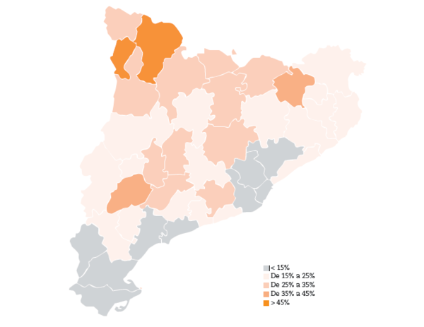

Source: Sindic de Greuges 2007, their own elaboration based on data from the Catalan Department for Education and the Census.
Figure 2 percentage of household using formal childcare arrangements, and level of public childcare coverage, by time periods.

Figure 3 Percentage of children participating in formal childcare, by family income levels and time period

Figure 4 Parents’ education level, by income groups
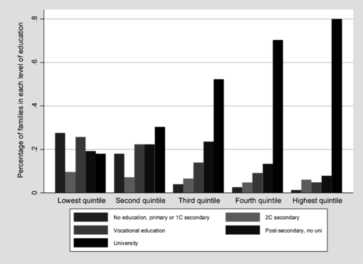

Figure 5 Mother’s working pattern, by income groups
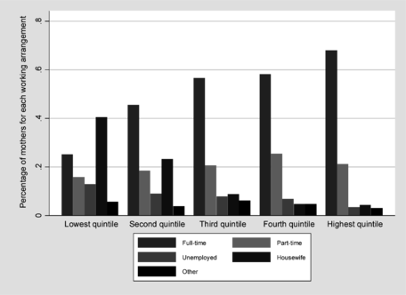

Figure 6 Education and number of hours worked as potential causes of heterogeneity between low-income and high-income part-timers and low-income and high-income housewives.
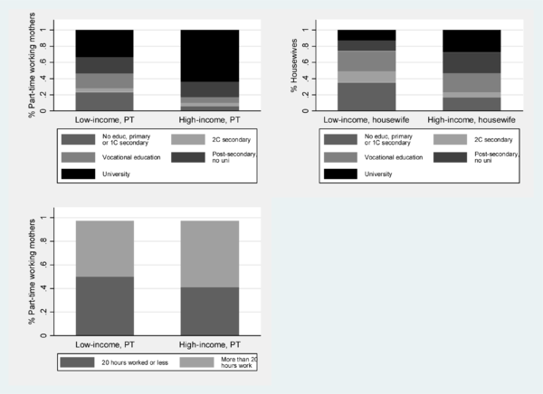

Note: Upper-left: the figure shows the education levels of part-time working mothers, for low-income and high-income families. Upper-right: the figure shows the education levels of housewives, for low-income and high-income families. Bottom-left: the figure shows the number of hours of part-time working mothers, for low-income and high-income families.
Document information

Published on 11/05/18
Accepted on 08/04/18
Submitted on 28/02/18
Licence: CC BY-NC-SA license
