On application of the finite point method to heat and elasticity problems

Abstract

A stabilized version of the Finite Point Method (FPM) is presented. A source of instability due to the evaluation of the base function using a least square procedure is discussed. A suitable mapping is proposed and employed to eliminate the ill-conditioning effect due to directional arrangement of the points. A step by step algorithm is given for finding the local rotated axes and the dimensions of the cloud using local average spacing and inertia moments of the points distribution. It is shown that the conventional version of FPM may lead to wrong results when the proposed mapping algorithm is not used.

It is shown that another source for instability and non-monotonic convergence rate in collocation methods lies in the treatment of Neumann boundary conditions. Unlike the conventional FPM, in this work the Neumann boundary conditions and the equilibrium equations appear simultaneously in a weight equation similar to that of weighted residual methods. The stabilization procedure may be considered as an interpretation of the Finite Calculus (FIC) method. The main difference between the two stabilization procedures lies in choosing the characteristic length in FIC and the weight of the boundary residual in the proposed method. The new approach also provides a unique definition for the sign of the stabilization terms. The reason for using stabilization terms only at the boundaries is discussed and the two methods are compared.

Several numerical examples are presented to demonstrate the performance and convergence of the proposed methods.

1. INTRODUCTION

Advances in computer science and technology in the past three decades have lead to development of robust numerical methods such as Finite Element (FE) and Finite Volume (FV) methods in computational mechanics. Although these two methods are still receiving considerable attention and every year thousands of papers are published, the idea of using simpler methods is also the subject of many research works. This is mainly because the mesh generation part of the solution has shown to be a very time consuming challenge especially in application of FE and FV methods to three-dimensional problems. In this way, the idea of developing methods requiring no mesh has led to emerging of a new class of so called “Meshless” methods.

A survey in the literature shows that the first application of the Meshless methods, proposed by Lucy [1], was in the solution of astrophysical problems. The method, called Smooth Particle Hydrodynamics (SPH), was further developed and studied in some research works by Monagham [2,3]. A fast growing attention on the subject can be seen in the 1990’s when a number of methods were proposed. A good survey, up to the date, can be found in Reference [4].

The term “meshless” has been used to convey the idea of using no grid of elements. Some early versions of the method uses background meshes to perform the integration required in the solution and thus are not “truly meshless” methods. Considerable attempts to propose truly meshless methods were made during the past decade. Today, researches are convinced that the approach is useful for some class of problems, e.g. crack propagation, for which the finite element solution requires subsequent remeshing.

Meshless methods can generally be classified in two major categories. The first one based on a weak integral form of the governing equations and thus requires a suitable integration scheme. Meshless methods based on collocation schemes can be included in the second category. For example the finite difference method on irregular grids falls within the latter category.

Among the methods using the weak formulation we find the Diffuse Element (DF) method proposed by Nayroles et al [4]. In DF the unknowns are approximated through a Moving Least Square (MLS) procedure and an integral form of the differential equations are satisfied in a Galerkin form of weighting.

Belytschko and co-workers followed a rather similar approach called Element Free Galerkin (EFG) method [5]. The main difference between DE and EFG lies in the computation of the derivatives of the functions. In the DE method, some terms of derivatives of the shape functions are ignored while in the EFG full derivatives of shape functions are used which leads to more accurate results. In both methods, numerical integration requires a mesh of quadrature points in the background of the domain and therefore they are not truly meshless methods.

In a series of papers written by Liu and co-workers, a new concept, referred to as Reproducing Kernel Particle Method (RKPM), for producing consistent base functions for the interpolation of unknowns was presented [6-10]. On the same line, the Partition of Unity (PU) method proposed by Babuška and Melenk should also be mentioned [11,12]. Application of hp-cloud method, proposed by Duarte and Oden, on a grid of points is also considered as a meshless approach [13]. Other meshless methods, called Meshless Local Petrov-Galerkin (MLPG) and Local Boundary Integral Equation (LBIE), using moving least square approximations were proposed by Zhu et al [14] and Atluri and Zhu [15,16], respectively. On the same basis, De and Bathe presented the method of finite spheres [17].

In the context of collocation methods early research by Jensen in 1972, as a promotion of the finite difference method, can be categorized within the class of meshless methods [18]. In this work the derivatives of a function are approximated in terms of its nodal values by means of two-dimensional truncated Taylor series. This was an important step towards approximation of functions on irregular grids of nodes.

Another finite difference method on arbitrary grids was proposed by Perrone and Kao in 1975 [19]. Again, truncated Taylor series were used for approximating the unknown function. A specific procedure for selection of a set of neighboring nodes in the cloud was introduced to guarantee the accuracy and stability of the results in the least square procedure.

One of the major drawbacks of the FD method on irregular grids is the instability of the results. Thus, the convergence of the solution is highly sensitive to the geometry of the cloud and to the selection of the nodes around the master node. Stabilization of the FD method has therefore been the goal of several research works. Demkowicz and co-workers published an article in which a new criteria was proposed for selection of neighboring nodes [20]. It was proven that satisfying such criteria leads to convergent results when the FD method is applied on irregular grids. Another attempt for stabilizing the method was made by Liszka and co-workers, in 1996, who developed a new version of the FD method called hp-Meshless cloud method [21]. This method uses Moving Least Squares (MLS) to fit a truncated Taylor series on a set of nodal values. To solve the instability problem, a new version of the moving least square approximation (Hermitian type of approximation) was developed in which the derivatives of the unknown function in the normal direction to the boundary were considered as additional variables for the boundary nodes. This technique improves the quality of the approximation in the vicinity of the boundaries.

The Finite Point Method (FPM), proposed by Oñate et al in 1996 for solution of fluid flow problems [22], uses a Weighted Least Square (WLS) scheme for approximating the unknown function. The governing differential equations and the boundary conditions are satisfied using point collocation. In this research an upwinding approach was used as stabilization procedure. The application of the method to advective-diffusive fluid problems can be found in [23]. A residual stabilization technique was later used as another alternative by the same authors [24]. The technique was a basis for development of a stabilized version of the FPM using Finite Calculus (FIC) proposed in 1998 [25]. The FIC method is not only useful for stabilization of results in FP, FD and FE methods but also has a wide range of applications in computational mechanics [26].

An overall view of the possibilities of the finite point method to incompressible flow problems was presented in [27]. The reader is referred to a recent work performed by Löhner and co-workers for compressible flow problems as another attempt for achieving stabilized results using the finite point method [28].

For elasticity problems, Oñate et al presented a finite point method using the FIC technique in order to overcome the instability of the results obtained from the conventional version of FPM [29,30]. This stabilization procedure dramatically improves the convergence and accuracy of the method.

Although meshless methods based on weak form formulations are shown to be robust, they are very time consuming due to the integration required in the formulation. On the other hand, meshless methods based on point collocation, though not fully stable, are very fast and have received considerable attention. In this paper we shall focus on the finite point method and propose two simple remedies to overcome the instability problems.

The layout of the paper is the following. After a brief review of the least square procedures, we propose a mapping scheme to reduce the problem of ill-conditioning of the coefficient matrix which sometimes occurs due to non-isotropic arrangement of the points. The procedure of polynomial fitting will be followed by a modified version of the method consistent with the mapping scheme and suitable for application of the Dirichlet boundary conditions.

In the section of solution methods, we shall propose a simple correction, inspired from the general form of the weighted residual approach. The method is in fact a reinterpretation of the Finite Calculus procedure using a special form of the characteristic length. In a detailed discussion we compare the similarities between the two methods. Several examples are given to demonstrate the performance of the proposed FP methods.

2. APPROXIMATION METHODS

In this section we shall give an overview to the approximation used to construct the base functions. The first step is choosing an appropriate polynomial.

2.1 The polynomial used

As mentioned in the previous section, the first stage for the numerical solution of differential equations is the approximation of the unknown function in terms of a set of nodal values. One of the simplest and oldest approximation methods, first used in finite difference methods on irregular grids, is based on truncated Taylor series.

Let the function be continuously differentiable up to the required order. Its expansion in a two-dimensional space can be written as

(1)

Here and are suitable local coordinates. The function might be approximated by a finite number of terms of a Taylor series as follows

(2)

where is a measure of the average spacing between nodes and is the order of the approximation.

On view of (2) the unknown function may be approximated by a complete polynomial as

(3)

The coefficient values for a finite region around the -th master node are determined by imposing the following condition at a finite number of nodes

;

(4)

where is the number of nodes selected in the vicinity of the -th master node. Obviously, to obtain a square system of equations, must, at least, be equal to the number of monomials in (3). Unfortunately, the application of the method on some grids may lead to a singular or ill-conditioned system of equations. Some of such arrangements are shown in Figure 1. To tackle the problem, a least square procedure with the number of nodal unknowns greater than the number of monomials is usually employed. However even in such least square fitting, there is not a guarantee to avoid an ill-conditioned matrix. A detailed description for this class of approximation methods is given in the next section.

Figure 1. (a) Singular arrangement of nodes for fitting a quadratic polynomial; (b) Ill-conditioned arrangement of nodes.

2.2 Weighted Least Square Method

Least square methods are useful procedures for approximating the unknown functions in meshless methods. The bases of the method are given next.

Assume function is to be approximated in domain with nodal points. The approximate function in sub-domain in vicinity of the -th node with neighboring nodes (see Figure 2) may be written as Equation (3) or as

(5)

where is a vector of base monomials and is a vector of coefficients.

Figure 2. (a) Domain with nodes; (b) Sub-domain with nodes.

As mentioned in the previous section, the values of for the -th cloud are determined from the satisfaction of (4). Assuming that generally is greater than , then satisfaction of (4) requires a least square procedure, which leads to minimization of the following discrete norm

(6)

Where is a suitable weighting function for the -th cloud.

Note that for each cloud a local coordinate system is defined, the origin of which is located at the master node of the cloud (node number ). The approximate function for the cloud is obtained on such a coordinate system.

The discrete norm in equation (6) is minimized as

(7)

which yields the following system of equations

(8)

where

(9)

and

(10)

Solution of (8) gives

(11)

Depending on the arrangement of the nodes and the weighting function used in the cloud, matrix may become singular (see Figure 1 for instance). Here we will assume that is regular so that is available. In case that the node arrangement is directional, matrix may become ill-conditioned but with the aid of appropriate cloud dimensions, as suggested in the forthcoming subsections, this effect can be reduced.

The approximation for the -th cloud is obtained by substituting Equation (11) in (5) as

(12)

where is a matrix containing the shape functions for each cloud.

The term ‘cloud’ refers here to a circular or rectangular area, with the center at the master node, containing at least the minimum number of points required for the weighted least square (WLS) procedure. The way we allocate an area to a master node will be described later.

A primary cloud is chosen first with some selected points. However, the primary cloud is just used for further process in order to find the final configuration of the main cloud over which the least square procedure is performed. The selected points in the final cloud might be slightly different (due to aspect ratio) from those selected in the primary cloud. The weighting function is defined over the final configuration of the cloud.

There is an important criterion for selecting the weighting functions in (6). The maximum value of the w_i should, preferably, occur at (the master node of the cloud) to capture the nodal value, or at least to obtain a sufficiently close value, to be used at the Dirichlet boundary condition. It might be argued the necessity of assigning the maximum weight to the master node and some may prefer to let this happen at the vicinity of the master node. This assumption intuitively emerges from the fact that the approximate information at the master node is to be extracted, preferably, from the information available at the node, as a first priority, and from the rest of the points in the cloud with less priority as the weighting indicates. If the maximum weighting is assigned to other places, there will be no guarantee for such extraction of information when the point distribution around the master node is dense. However, what we shall explain in the forthcoming sections can be applied to such cases with no loose of generality.

Figure 3. Normalized Gaussian weight function.

In this paper we shall use a truncated Gaussian weighting function, as Figure 3 depicts, defined by

(13)

Where denotes the distance between the point and the master node. Also and denote two distances proportional to the distance between the master node and the most remote point in the cloud, i.e. and . The weighting function is, in fact, suitable for circular clouds. This weighting was suggested in reference [5] and later used in many studies [15,16,22]. For rectangular clouds the product of two weighting functions written along the two principle directions may be used. It may be noticed that the weighting at the most distant node can be controlled by parameters and in the weight expression. This might be interpreted as choosing a larger fictitious area, containing the selected points (although it may cover more points than those selected). In this paper we have used and .

It is obvious that since the approximation in the least square procedure is based on the minimization of an error norm, the approximate function does not have the selectivity property. In other words

(14)

This property creates an inconsistency to satisfy the Dirichlet boundary conditions and this is a source of instability when the meshless procedure is used with a weak formulation [6-10]. Although, for point collocation methods the deficiency has not been reported, we recommend to employ the modified form of the WLS method as defined in a next section.

2.3. Selection of clouds

Several cloud definitions may be given for a collection of nodes. In general, the geometry of the cloud should follow the distribution of the nodes. In other words, for isotropic distributions circular or square clouds are preferred, while for non-isotropic distributions the use of elliptic or rectangular clouds may give better results (Figure 4).

Figure 4. Cloud selection for a typical master node: (a) Isotropic distribution of nodes; (b) Non-isotropic distribution of nodes.

Here we shall briefly describe the cloud selection for both isotropic and non-isotropic distribution of points.

2.3.1 Isotropic point distribution

When the points are distributed with a uniform density a circular or square cloud may be used. The dimension of the cloud depends on the number of points required for polynomial fitting. For instance, if circular clouds are used, the procedure starts by choosing a minimum radius for each circle followed by a progressive increase of the radius until the required number of points, say twice as many as the monomial terms, is available. The dimension of the first circle and the rate of the enlargement are usually chosen by average spacing of the points.

A general adaptive solution may start from an isotropic point distribution. As the point insertion goes on, a directional point distribution may be observed where the variation of the function is very high. Therefore, in order to generalize the application of any meshless method, it is essential to devise a suitable scheme for handling such arrangements of points.

2.3.2 Non-isotropic point distribution

When the point density is directional, the application of circular or square clouds may lead to an ill-conditioning or even singular coefficient matrix in Equation (9). Even in robust numerical solutions, such as the FEM, similar situations may happen when elements with high aspect ratio are used and the shape functions are defined in terms of global non-scaled coordinates. Nowadays, it is well understood that defining the shape functions in local normalized coordinates solves the problem. In this section, we propose a remedy for such situations in meshless methods, based on an analogy with the FEM.

Application of normalized clouds

As the anisotropy of the grid increases, matrix in Equation (9) becomes ill-conditioned and the quality of the approximation deteriorates. In the classical least square procedure, i.e. with weights equal to unity, the elements in , as is seen in (10), are proportional to the powers of the relative distances between the master node and the other nodes (recalling that the origin of the coordinates has been placed at the master node). In a WLS procedure, the weights in the expression of may accelerate the dimension dependency of the solution. We note that when circular clouds are used this effect is worse than in rectangular clouds. The reason is that in circular clouds the weighting is defined in terms of the absolute maximum distance between nodes.

In order to prevent such undesirable effect, a mapping may be used to compute the values of the shape functions and their derivatives with a higher quality. A fictitious square domain is chosen as an intermediate cloud and all points within the main cloud are transferred to such fictitious isotropic sub-domain. The least square procedure is then performed on the normalized cloud. This may be interpreted as preconditioning the matrix in a consistent manner.

Figure 5. (a) Non-isotropic grid; (b) Cloud of a typical node; (c) Normalized cloud of the typical node.

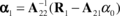
Let us consider a cloud with the correct point density. A local coordinate system is chosen with origin at the master node where (see Figure 5)

,

(15)

Here and denote maximum distances along x and y measured from the master node and the exterior nodes in the cloud. The A and B matrices in Eq. (9) have now the following form in terms of the local coordinates

  ,       

where the weighting function is rewritten as

were we have used , and as usual , . Note that we are using a circular weighting function on a square cloud.

The coefficient matrix is not longer dependent on the cloud dimensions. The approximate function is also expressed in terms of the local coordinates as

(16)

provided again that exists, which means that the points should be properly distributed in the new square domain. If is still singular, the dimensions of the main cloud are successively altered, and the procedure is repeated with new selected points and repetition of the mapping, until a non singular coefficient matrix is obtained. If such strategy does not lead to a regular matrix, a point selection criteria, as used in [19] or [20], might be employed within the normalized cloud. According to our experience, usually there is no need to use any point selection criteria.

Having found the base functions, the derivatives with respect to the global coordinates may be computed by the chain rule

,

(17a)

or

, ,

(17b)

and so forth. The effect of such a mapping is illustrated in the following sample problem.

Sample problem

A rectangular cloud with 9 points, similar to Figure 5, is considered for the polynomial fitting. A second order complete polynomial with six unknown coefficients is to be fitted on nine values at the points. The least square procedure is performed using both non-normalized and normalized coordinates. It is desirable to recapture the unit value for the base function at the central node, as this will reproduce the nodal value after the fitting process. As an indication for the deterioration of the fitting process due to the aspect ratio dependency of matrix , in Table 1 the value obtained for the central base function of node 1 at the origin of the coordinates, i.e. at is monitored for different aspect ratios. It can be seen that the quality of the base function deteriorates when the aspect ratio increases and a non-mapped cloud is used. On the other hand, when using a mapped cloud the quality remains unchanged. It is noteworthy that in this sample problem we have used a weighting function with circular support on a rectangular cloud. The circular support function, i.e. a circle with radius of , passes over the corners of the cloud.

Table 1. Values of shape function at a master node with non-mapped and mapped clouds

	N(0,0) (non-mapped cloud)	N(0,0) (mapped cloud)
1.0	0.9677	0.9677
0.5	0.7546	0.9677
0.25	0.5516	0.9677

The fast deterioration of the fitting process quality is mainly due to the low values of the weights of points 3, 4, 5, 7, 8 and 9, in comparison with the weight of points 2 and 6, while decreases. For instance for the maximum weight for the six points at the upper and lower edges amounts to while for points 2 and 6 the weight values amount to which results in a ratio with logarithmic order of six. For a square cloud, the weight values at points 2, 4, 6 and 8 are equal to , which in comparison with the weight value at points 3 ,5 , 7 and 9 the ratio is of logarithmic order of three. In fact, when decreases the procedure resembles to fitting a second order polynomial using information from just three points. This is a physical interpretation of what happens within the weighting least square procedure.

Looking into the sample problem in more detail, one may write Equation (9) in partitioned form as

where the first unknown , corresponding to the approximation at master node, in Equation (3) is split from the remaining part of . Now if the polynomial coefficients are determined as

  ,          

it can be concluded that the accuracy and value of the approximation at the master node is dependent on the regularity of . Denoting the weight values at points 2 to 9 in Figure 5 as , and , a parametric form of matrix for the above sample problem is

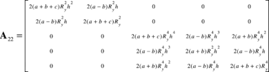
where . It can be seen that when decreases matrix becomes ill-conditioned, irrespective of the weight values (note that , and ).

Also, even if the aspect ratio is not so large, the weight values can accelerate the ill-conditioning of A₂₂ particularly when one of the weights, or , becomes much larger that the other two, i.e. . In that case the third and fifth rows of above matrix tend to become a multiple of each other. This is the case, for instance, when in which is of six logarithmic order larger than the other two weights. Of course, this is not the case for a square cloud in which both and are equal and are of just three logarithmic orders larger than .

Clearly, the ill-conditioning may also happen in a square cloud if (the weight value at the corner points in Figure 5) becomes very small. This means that we are fitting a second order polynomial on just five points. We note that the user can control the weight values at the corner points by allocating different values to the parameters in the expression of the weights given previously.

It can also be concluded that the effect of the aspect ratio on decreasing the quality of the least square procedure increases when higher order polynomials are used.

In above example we have just focused on values obtained at a master node as an indicator. The reader may notice that the non zero matrix in includes coefficients of second order monomials, and therefore, when ill-conditioning happens all the corresponding coefficients are of poor accuracy. This leads to inaccurate results in problems with second order differential equations for instance, letting alone the inaccuracy of the solution at the Dirichlet boundary.

We also note that even if a modified version of WLS is employed so that the recovered value at the central point becomes unity, as recommended in the next subsection, the problem of ill-conditioning of the coefficient matrix remains unless a normalized cloud is used.

Before explaining the way the main cloud is selected, it is worthwhile to complete the mapping by a simple rotation in local normalized axes.

In case the point distribution is not along the global axes, the governing direction may be sought by finding the principal axes of the point pattern. This requires calculating the moments of inertia of the points assuming equal mass/weight for the points as

, ,

(18)

The corresponding angle is then obtained as

(19)

The first derivatives, for instance, in global coordinates may be evaluated by

,

(20)

with and being the cloud dimensions in the new coordinates.

Figure 6. (a) A primary circular cloud with points, (b) Main cloud is built through finding the principal axes and proper aspect ratio, (c) normalized cloud with circular weight support.

Now the question of the appropriate cloud selection must be addressed. For a very irregular grid of nodes, the cloud selection and mapping process may be summarized as follows (see Figure 6 for details):

- A number of the nearest points to the master node, say the minimum number required for the final least square procedure, are selected. The distance between the master node and the most remote point is calculated. A circular area is considered of radius equal to the calculated length. The area may cover more points than those selected at the beginning of the step. The circular area may be viewed as a primary cloud. It should be noted that the cloud chosen in this step is not the one on which the least square is performed. In fact, such a primary cloud is only intended for evaluating the local governing directions of the point distribution.

• The angle of the principal axes of the selected points is found through relations (18) and (19).

• The average spacing of the points is determined along the two new axes. This can be performed by sorting out the node numbers with respect to their new coordinates so that and for the direction and once more, and for the direction of . Now distinct locations of point concentrations, along and , must be found. In our work we have used a very simple approach for finding the point concentration locations, although more sophisticated (and expensive) methods may be applied. All sequentially ordered coordinates having a difference less than a specified tolerance, e.g. and with being the number of points, are considered as a point concentration and the average of the coordinates is taken as their representative. Assuming that and are the number of points concentrated along the two axes, clearly and , the average point spacing is be found as

,

where and denote the coordinates of the points concentrated along the rotated axes and , respectively.

• A primary rectangular domain with aspect ratio of is built on the master node (with center at the master node and edges parallel to the rotated axes). The dimension of the rectangle is increased sequentially, maintaining the aspect ratio, until a minimum number of points fall into the cloud. The sequence length may be chosen as one of the average spacing calculated. The selected points, at this stage, are not necessarily the same as those selected at the first step.

• The dimensions of the cloud along the two axes, to be used in the normalization procedure, are calculated as and .

• The polynomial fitting is performed using the new positions of the points in the normalized coordinates. If the coefficient matrix is singular, the rectangular cloud selected in the previous step, i.e. the last one with aspect ratio of , is further enlarged and some new points are added to the first set. The procedure is repeated until a non singular coefficient matrix is attained. Generally, there is no need to repeat the first step and change the dimensions of the primary cloud, as the information required for the approximation at the master node is taken from the closest points whose distribution has been already calculated. However, if the number of points added is much larger than that of the first set, say three times as large, it might be preferable to repeat the cloud selection process with a larger value for the minimum number of points, or a sequence of enlargements with a sequence length of .

Once the approximate functions over the cloud at each master node are found the shape function derivatives with respect to the global coordinates are evaluated through Equations (20).

In section 4 we present an example to show that without using the above procedure, especially when the arrangement of the points is directional, wrong answers may be obtained.

2.4. Modified Weighted Least Square Method

We have shown in previous section that using normalized local coordinates not only reduces the instability induced by the fitting processes, but also improves the accuracy of the procedure near the master node so that the selectivity property of Eq.(14) is proposed achieved. In this section a modified version of the weighted least square method is recommended, in which the deviation from unity is recovered and the approximate function passes exactly by the central node of each cloud. A similar method was presented in reference 21 for direct calculation of derivatives of the approximate function in global coordinates. The method is revisited here for evaluation of the base functions in the normalized cloud to be differentiated later with respect to the global axes through relations (20).

Assume that for the -th node a cloud of neighboring nodes is defined. The local number of the master node is set to be unity. The approximate function, in the normalized coordinates, may be written as

(21)

In other words

(22)

An example of in above equation is

; (For quadratic approximation)

(23)

In order to determine the values, we substitute equation (22) into (7). Hence

(24)

As the error for node 1 is equal to zero, it does not enter in the above norm.

The discrete norm of equation (24) is minimized as follows

;

(25)

which as before leads to

(26)

where

,

(27)

and

(28)

One can use the following equation to replace by

(29)

with being the following transformation matrix

; ,

(30)

Equation (26) may be rewritten as

(31)

which gives

(32)

Once again we have assumed that the point distribution is such that is available. Substitution of (32) into (22) gives

(33)

On the other hand we have

(34)

where

(35)

Finally we have

(36)

where is the shape function matrix for the -th cloud.

The procedure gives slightly different results for the derivatives of the functions when it is used in the collocation formulation. The reader will notice that the method differs from a simple shifting of the polynomial fitted in (13) since the number of variables in the least square procedure is less.

3. SOLUTION OF BOUNDARY VALUE PROBLEMS

Having found appropriate base functions for interpolation of the unknowns, a suitable solution method should be chosen. The mathematical model is usually summarized as a set of differential equations

(37)

which is to be satisfied with the following boundary conditions

(38a)

and

on

(38b)

where ${\boldsymbol {\cal {A}}}$ and ${\boldsymbol {\cal {B}}}$ are differential operators for the governing equation in the domain and the Neuman boundary conditions, respectively. The domain is a subset of in which equation (37) is to be satisfied and is the boundary of the domain on which equations (38a) and (38b) are to be satisfied.

To solve the problem numerically, we start from the general weighted residual expression. Thus

(39)

in which , and are suitable weighting functions arranged in diagonal matrices. If the equation holds for any arbitrary weighting functions, then it follows that . But as this is not generally possible, depending on the choice for the set of weighting functions, will be an approximate of . The essential boundary conditions are usually satisfied exactly (see section 2.4) and thus the main integral equation is

(40)

Now the weighting functions are to be chosen so that the number of equations and nodal values be in balance to obtain a system of equations as

(41)

Depending on the choices for and different numerical solutions will result. To explain our interpretation of the weighted form of (40), the weak formulation will be written next.

Weak formulation

The weak formulation is obtained when an integral by parts is performed of the integral containing the operator ${\boldsymbol {\cal {A}}}$ giving

(42)

Where ${\boldsymbol {\cal {A}}}_{1}$, ${\boldsymbol {\cal {A}}}_{2}$ and ${\boldsymbol {\cal {C}}}$ are suitable operators extracted from the integration by part and consistent with operator ${\boldsymbol {\cal {A}}}$, for instance ${\boldsymbol {\cal {A}}}\equiv {\boldsymbol {\cal {A}}}_{1}{\boldsymbol {\cal {A}}}_{2}$. In boundary value problems, usually, operators ${\boldsymbol {\cal {B}}}$ and ${\boldsymbol {\cal {C}}}$ contain similar terms so that they can be eliminated when the weighting functions are selected by choosing

(43)

which leads to elimination of the natural boundary conditions. Now, if the Galerkin method is employed, i.e. , the approximation is said to be optimal (for elliptic problems). Indeed, it can be shown that in such a case the solution is equivalent to minimization of a suitable norm of the approximate solution error with respect to nodal variables [32].

The reader will notice that if we substitute Equation (43) into (40) gives

(44)

It should be noted that as the base functions and the weighting functions are defined on small sub-domains few of them have edges at the boundaries. Therefore

(45)

and

(46)

Finite Point Method as a Subdomain or Point Collocation Method

Now assuming that is small and is chosen, similar to a sub-domain collocation, such that

(47)

Then

(48a)

and

(48b)

In above, a “bar” is used to indicate evaluation of the average of the function over and is the projection of on the boundary. Equations (45) and (46) can be rewritten as

(49a)

and

(49b)

Since is assumed to be very small, the average values on may be taken as proportional to the corresponding values at the master node and thus

(50)

Here denotes the number of the master node and and are appropriate coefficients. Assuming that is so small that the average values and the master node values are of the same sign, then Equations (49) can be written as

(51a)

and

(51b)

Above equation is equivalent to using a collocation method considering the area and the edge length influenced by the node as the weights.

We notice that in Eq.(51b) the equilibrium equations and the Neumann boundary condition appear with opposite signs in a single equation. It may be also observed that in Equation (51b) the ratio of the sub-domain to its projection to the boundary, i.e. a characteristic length, is of more importance than the absolute values. Therefore, to solve the problem using a finite number of points, the smallest area around a point is chosen in order to evaluate an appropriate characteristic length. The reader will notice that such a characteristic length is only used at the boundary nodes.

In summary, the following equations must be solved for nodes at inside or at the boundary of the domain:

(52a)

(52b)

In above and are the areas associated to the node and the nearest neighboring points as shown in Figure 7, and and are their projections on the boundary. Also is a suitable factor. Our studies show that and are the best choices for elasticity and Poisson’s equations, respectively.

Figure 7. Evaluation of and values for Neumann boundary nodes: point 1 is the closest inside point to master node , and are the projections of constructed sub-domains and to the boundary of the domain.

Analogy with Finite Calculus (FIC)

A similar set of stabilized discretized equations can be obtained using the finite calculus (FIC) method proposed by Oñate [25]. The FIC method has been used for stabilization of the finite point method [29,30] using a generalization of the method originally proposed for convection-diffusion and fluid flow problems [25]. To illustrate the analogy between the two methods, in this section we shall overview some features of FIC method. This will provide another interpretation for effectiveness of adding two residuals in one set of equations.

The idea of the FIC method is to apply the basic thermodynamic balance laws not to an infinitesimal domain but to a domain with finite dimensions. This leads to a modified system of governing equations which contain additional terms than the standard differential equations of the infinitesimal theory.

Let represent the standard differential equations at a point in two dimensional space. The modified governing equations obtained with the FIC method can be written as [25,26]

(53)

where is a characteristic length vector whose direction is to be specified. Several stabilization methods may be interpreted by choosing appropriate magnitude and direction for . For example, in fluid flow problems a Streamline Upwind Petrov-Galerkin (SUPG) may be recovered if is taken in direction of the velocity , i.e.

(54)

Other possibilities are discussed in details in [25,26].

The FIC approach if applied at the boundaries with the Neumann condition results in the following modified equation [25]

(55)

where is the unit normal to the boundary. This equation may be compared with Equation (51b). Here we note that depending on the direction of h the stabilized boundary conditions can be written in two forms:

(56a)

and

(56b)

where .

When the stabilization is generalized to elasticity problems the choice of the sign in the equation remains unsolved.

Note that the first form of Equation (56) is analogous to that of Equation (51b) deduced from the weighted residual formulation. Also, as discussed in the previous subsection, the choice of (56b) in which both the equilibrium equation and boundary condition residuals appear with similar signs is not consistent with the optimal solutions. Hence the form of Equation (56a) should be used in practice.

Incidentally in references 29 and 30 the correct choice of signs in Equation (56a) was selected and it was shown that the resulting FPM gave stable results for a variety of problems. It is noteworthy to mention that our formulation shows that there is no need to add any additional terms for the residual equations at the inside nodes. This coincides with the observation made in [29] and [30] in which adding an stabilization term to the equations within the analysis domain, similar to Equation (53), has been recognized to be not effective.

Another difference with the FIC stabilization procedure presented in [29,30] is the way we select the characteristic length parameter via Equation (52b).

4. NUMERICAL RESULTS

In this section we present some numerical examples to show the reliability of the method proposed in this paper. A quadratic interpolation has been used in all problems.

Simply supported beam under uniform load

A two dimensional simply supported beam subjected to uniform load has been solved under plane stress condition. In order to demonstrate the effect of using normalized and rotated coordinates the point distribution is selected first as the pattern shown in Figure 8-b. The displacements obtained using the proposed approach are given in Figure 9. It can clearly be seen that without using the normalized and rotated coordinates some wrong answers are obtained. From this example on we shall use the mapping algorithm to minimize the effect of instability due to polynomial fitting.

Figure 8. (a) Simply supported beam under uniform load; (b) skew grid; (c) cartesian grid.

Figure 9. Vertical displacement at the top fiber of simply supported beam.

The problem is also used to study the convergence rate of solution when the proposed stabilized Finite Point Method is employed. The simply supported beam has been solved using a series of regular point distributions one of which is depicted in Figure 8-c. Although not shown in the figure, to prevent singularity effect at the supports, two parabolic distributions of shear stresses equilibrated with the distributed loads, are considered. Only one node is restrained at each end to eliminate rigid body motion. Maximum deflection and flexural stress are used to evaluate the accuracy of the solutions. For presentation of the errors, the exact values for the quantities are obtained from a two dimensional elasticity solution given by Timoshenko and Goodier [33] for modeling of an equivalent beam problem. The problem solved in the reference requires a longitudinal stress distribution which varies with a cubic polynomial along the height and is constant along the length of the beam and also has zero resultant axial force and bending moment. Such stress distribution may be added, as additional tractions, at the two ends. However, in our model we have neglected the effects of the longitudinal stress distribution because of two reasons. Firstly, due to Saint-Venant’s principle the effect of such additional tractions is negligible at the middle of the beam (as also discussed in [33]). Secondly, even in the exact solution, the discrepancy from neglecting such stress distribution, considering the dimensions shown in Figure 8-a, is about compared to the exact value . This error is less than the accuracy we need for presentation of performances of the conventional and modified versions. Nevertheless, we have used the relations given in [33] for the exact values for our presentation and this means that we obtain around more error which leads a shift in stress error diagram considering the range of the error shown in figures. Figures 10-a and 10-b show the results of the errors for both the conventional and the stabilized versions of the Finite Point Method. It can be seen that the monotonic convergence is lost when the solution is performed with no stabilization terms. However, when the boundary described in Section 3 is used, i.e. when the equilibrium residual terms are added to the traction residuals, monotonic convergence is achieved.

Figure 10. Solution of simply supported beam under uniform load using conventional and stabilized versions of FPM; (a) Error of maximum vertical displacement; (b) Error of maximum tensile stress.

The variation of deflection along the length and variation of normal stress along the height of the beam for various numbers of degrees of freedom are given in Figures 11-a and 11-b. In Figures 10-a and 11-a the exact deflection of the beam is calculated from the relation given in [33] taking into account the effects of shear deformations.

Figure 11. Simply supported beam under uniform load: (a) Distribution of vertical displacement along central fiber of the beam (y=0.5); (b) Distribution of normal stress along the central cross section of the beam (x=4).

Laplace equation in a unit square

To demonstrate the performance of the standard and stabilized versions of FPM for problems with scalar differential equations, solution of a Laplace equation as

 ,             ,         

on a square domain shown in Figure 12-a is considered as another benchmark problem. The Dirichlet boundary conditions, at and , and Neumann boundary conditions, at and , are defined in accordance with the following exact solution

Two sets of regular and irregular point distributions have been chosen for the numerical solutions. In all cases the mapping algorithm presented in Section 2.3.2 has been used and thus the main difference between the versions lies in the application of the stabilization method via the correction of the boundary residuals.

Figure 12. Laplace equation in a square domain: (a) The domain; (b) Solutions by conventional and stabilized versions of FPM.

To demonstrate the deviation of the answers from the exact values in all points, the following error norm is defined

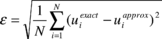
Where and are the exact and approximate values of u_i and is the total number of discrete values.

The results obtained using the standard FPM (Figure 12-b), clearly demonstrate the lack of monotonic convergence specially for irregular patterns. It can be seen that when the stabilization presented in Section 3 is applied, the convergence is improved as Figure 12-b depicts.

It is worth to compare the overall rate of convergence for regular grids of nodes in Figures 12-b. It is observed that the convergence rate of the stabilized version is slightly less than that of the conventional FPM. The reason may lie in the fact that the stabilized version is much closer to an optimal solution than the original version. In fact, in a nearly optimal solution, the error density distribution is expected to be uniform over the domain. This means that the error at the boundaries propagates within the domain in the improved version and thus the overall accuracy appears to be deteriorated (the reader will note that the ratio of interior node number to the total number of nodes increases when the mesh becomes finer). For irregular grids the same discussion seems to be valid if the first non monotonic part of the curves are put aside and the convergence rates at the last three points are compared. In any case, an important conclusion is the elimination of the sharp upward jumps appearing in the conventional (non stabilized) FPM solutions.

A cantilever beam with an end load

A two dimensional cantilever beam, shown in Figure 13-a, is solved under plane stress condition. The problem has been solved as a benchmark problem in many references [15, 16 29 and 31]. The exact solution can be found in literature [33].

 ,

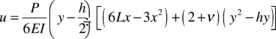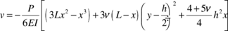
Where and are displacement components along and , is Poisson’s ratio, is elasticity modulus, and are height and length of the beam and . In this example we use , , , and . The end load is the resultant of a parabolic distribution of the shear stress. The results are obtained for regular and irregular point distributions. Here again to prevent singularity at the fixed end, a parabolic distribution of shear stresses is considered and just one point is restrained in order to eliminate the rigid body motion in the vertical direction. All horizontal displacements are restrained at the fixed end and the prescribed values are obtained from the exact solution.

Figures 13-b and 13-c show the results for a regular point distribution when no stabilization is used for the boundary points. The errors in these figures represent error norms, as defined in the previous problem, for each component. Similar to the previous example the convergence rate is not monotonic. However, when the stabilization described in Section 3 is used, a major improvement is observed and the rate of convergence becomes monotonic. This can clearly be seen in Figures 14-a and 14-b.

Figure 13. Cantilever beam under unit end load. Solution with conventional FPM; (a) geometry; (b) Error norms for each component of displacement field; (c) Error norms for each component of stress field.

Figure 14. Cantilever beam under unit end load. Solution with stabilized version of FPM; (a) Error norms for components of displacement field; (b) Error norms for components of stress field.

Figure 15-a depicts the beam deflection for various solutions. The stress distribution of the shear stress on a cross section at the mid span is given in Figure 15-b.

Figure 15. Cantilever beam under unit and load; (a) Distribution of vertical displacement along central fiber of the beam (y=0.5); (b) Distribution of shear stress along the central cross section of the beam (x=2.5).

Perforated plate under uniform tensile tractions

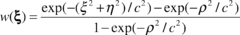
The final example is a plane stress solution of a perforated plate under tension. A quarter of the plate is solved using the tractions evaluated from the exact stress field (Figure 16). The exact solution of the problem is given below

where

,

In above equations, is the radius of the hole and are the polar coordinates of the points, with origin at center of the hole.

Figure 17 shows some of the results obtained from solution of the problem by application of the stabilized version of FPM presented in this paper.

Figure 16. Square plate under tension: (a) Infinite domain under tension; (b) A quarter of the finite domain under tractions; (c) A grid of nodes for solution of the problem.

Figure 17. Stabilized FPM solution of square plate with hole: (a) Error norms for components of displacement field; (b) Error norms for components of stress field; (c) Distribution of vertical displacement along line x=0; (d) Distribution of horizontal stress along line x=0.

5. CONCLUSIONS

The Finite Point Method was revisited in this paper. As for other collocation methods, numerical instabilities may appear from application of the standard (non stabilized) FPM. In this paper we have shown that polynomial fitting and treatment of the collocation equations near the boundaries are the two main sources of instability in the FPM.

Application of normalized clouds was proposed and examined through some examples. The method is similar to using mapping in the FEM and helps to overcome the ill-conditioning in the least square fitting especially when the point distribution in the cloud is directional. The study of a sample problem has shown that wrong answers might be obtained when the conventional form of polynomial fitting is used.

A stabilized version of the FPM using equilibrium residuals at the boundaries was presented. The formulation is consistent with the general formulation, which is usually used for weighted residual methods and leads to optimal solutions.

The analogy between the proposed stabilization method and the finite calculus (FIC) approach has been discussed. The conclusions can be summarized as

• Using the weighted residual approach shows that one of the remedies for the solution of instability in boundary value problems lies in the treatment of the Neumann boundary conditions.

• Stabilization based on an optimal solution via a weighted residual formulation has a unique form and the residuals of the equilibrium equations and the Neumann boundary conditions appear with opposite signs at the boundary equations where tractions are prescribed. Although the same form of stabilization may be obtained using the FIC method, the method proposed here helps to choose adequately the sign of the stabilization term at the Neumann boundary.

• A small area next to the boundary node, and its projection, may be used as the suitable weights in the proposed stabilization approach.

Examples show that the problem of non-monotonic convergence, usually observed in the application of the standard (non-stabilized) FPM, is effectively reduced using the stabilized formulation. Further studies on the mathematical basis of the method are needed in order to ensure that the monotonic convergence is always achievable.

References

[1] Lucy L. B., “ A numerical approach to the testing of the fission hypothesis” , Astron. J., Vol. 82,

No. 12, pp. 1013-1024,1977.

[2] Monaghan J.J., “ Why particle methods work”, SIAM J. Science and Statist. Comput., Vol. 3, No. 4,

pp. 422-433, 1982.

[3] Monaghan J.J., “An introduction to SPH”, Comput. Phys. Comm., Vol. 48, pp. 89-96, 1988.

[4] Nayroles G. B., Touzot and Villon P., “Generalizing the finite element method: diffuse approximation

and diffuse elements”, Comput. Mech., Vol. 10, pp. 307-318, 1992.

[5] Belytschko T., Lu Y. Y. and Gu L., “Element-Free Galerkin methods”, Int. J. Numer. Meth. Engrg.,

Vol. 37, pp. 229-256, 1994.

[6] Liu W. K. and Chen Y., “Wavelet and multiple scale reproducing kernel methods”, Int. J. Numer. Meth.

Engrg., Vol. 21, pp. 901-931, 1995.

[7] Liu W. K., Chen Y., Chang C.T. and Belytschko T., “Advances in multiple scale kernel particle

methods”, Comput. Mech., Vol. 18, pp. 73-111, 1996.

[8] Liu W. K., Chen Y., Jun S., Chen J.S., Belytschko T., Pan C. and Uras R. A., Chang C. T., “Overview

and application of the reproducing kernel particle methods”, Arch. Comput. Meth. Engrg: State of the

Art Reviews, Vol. 3, pp. 3-80, 1996.

[9] Liu W. K., Jun S., Li S., Adee J. and Belytschko T., “Reproducing kernel particle methods for

structural dynamics”, Int. J. Numer. Meth. Engrg., Vol. 38, pp. 1655-1679, 1995.

[10] Liu W. K., Jun S. and Zhang Y. F., “Reproducing kernel particle methods”, Int. J. Numer. Meth.

Fluids., Vol. 20, pp. 1081-1106, 1995.

[11] Melenk J. M. and Babuška I., “The partition of unity finite element method: basic theory and

applications”, Comput. Meth. Appl. Mech. Engrg., Vol. 139, pp. 289-314, 1996.

[12] Babuška I. and Melenk J. M., “The partition of unity method”, Int. J. Numer. Meth. Engrg., Vol. 40,

pp.727-7585, 1997.

[13] Duarte C. A. and Oden J. T., “An h-p adaptive method using clouds”, Comput. Meth. Appl. Mech.

Engrg., Vol. 139, pp. 237-262, 1996.

[14] Zhu T., Zhang J-D and Atluri S.N., “A local boundary integral equation (LBIE) method in

computational mechanics, and a meshless discretization approach”, Comput. Mech., Vol. 21,

pp. 223-235, 1998.

[15] Atluri S. N. and Zhu T., “A new Meshless Petrov-Galerkin (MLPG) approach in computational

mechanics”, Comput. Mech., Vol. 22, pp. 117-127, 1998.

[16] Atluri S. N. and Zhu T., “The meshless local Petrov-Galerkin (MLPG) approach for solving problems in elasto-statics”, Comput. Mech., Vol. 25, pp. 169-179, 2000.

[17] De S. and Bathe K. J., “ The method of finite spheres”, Comput. Mech., Vol. 25, pp. 329-345, 2000.

[18] Jensen P. S., “Finite difference techniques for variable grids”, Comput. Struct., Vol. 2, pp. 17-29,

[19] Perrone N. and Kao R., “A general finite difference method for arbitrary meshes”, Comput. Struct.,

Vol. 5, pp. 45-58, 1975.

[20] Demkowicz L., Karafiat A. and Liszka T., “On some convergence results for FDM with irregular

mesh”., Comput. Meth. Appl. Mech. Engrg., Vol. 42, pp. 343-355, 1984.

[21] Liszka T. J., Duarte C. A. M. and Tworzydlo W. W., “hp-Meshless cloud method”, Comput. Meth.

Appl. Mech. Engrg., Vol. 139, pp. 263-288, 1996.

[22] Oñate E., Idelsohn S., Zienkiewicz O. C. and Taylor R. L., “A finite point method in computational

mechanics-applications to convective transport and fluid flow”, Int. J. Numer. Meth. Engrg., Vol. 139,

pp. 3839-3866, 1996.

[23] Oñate E. and Idelsohn S., “ A mesh free finite point method for advective-diffusive transport and

fluid flow problems”, Comput.l Mech., Vol. 21, pp. 283-292, 1998.

[24] Oñate E., Idelsohn S., Zienkiewicz O. C., Taylor R. L. and Sacco C., “A stabilized finite point method for analysis of fluid mechanics problems”, Comput. Meth. Appl. Mech. Engrg., Vol. 139, pp. 315-346, 1996.

[25] Oñate E., “Derivation of stabilized equations for numerical solution of advective-diffusive transport and fluid flow problems”, Comput. Meth. Appl. Mech. Engrg., Vol. 151, pp. 233-265, 1998.

[26] Oñate E., “ Possibilities of finite calculus in computational mechanics”, Submitted to Int. J. Numer. Meth. Engrg., Sept. 2002.

[27] Oñate E., Sacco C. and Idelsohn S., “ A finite point method for incompressible flow problems”, Computing and Visual. Science., Vol. 2, pp.67-75, 2000.

[28] Löhner R., Sacco C., Oñate E. and Idelsohn S., “A finite point method for compressible flow”, Int.

J. Numer. Meth. Engrg., Vol. 53, pp. 1765-1779, 2002.

[29] Oñate E., Perazzo F. and Miquel J., “A finite point method for elasticity problems”, Comput. Struct.,

Vol. 79, pp. 2151-2163, 2001.

[30] Oñate E., Perazzo F. and Miquel J., “Advances in the stabilized finite point method for structural mechanics”, International Center for Numerical Methods in Engineering (CIMNE), Universidad Politécnica de Cataluña (Tech. Rep. 164), Presented in European Conference on Computational Mechanics (ECCM), München, Germany, 1999.

[31] Aluru N. R., “A point collocation method based on reproducing kernel approximations”, Int. J.

Numer. Meth. Engrg., Vol. 47, pp. 1083-1121, 2000.

[32] Zienkiewicz O. C. and Taylor R. L., “The finite element method”, 5^th edition, Butterworth-Heineman,

[33] Timoshenko S. P. and Goodier J.N., “Theory of Elasticity” (3^rd edn.) McGraw-Hill, New York, 1970.