Finding the optimum location in a one-median network problem with correlated demands using simulated annealing

Abstract

The one median location problem with stochastic demands can be solved as a deterministic problem by considering the mean of weights as demands. There are also some other approaches in consideration of this problem. However, it is better to find the probability for each node that shows the chance of the node being in the optimal location, especially when demands are correlated to each other. With this approach, alternative answers with their optimality probability can be found. In small networks with a few nodes, it is not so difficult to solve the problem, because a multivariate normal probability for each node should be calculated. But, when the number of nodes increases, not only do the number of probability calculations increase, but also, the computation time for each multivariate normal distribution grows exponentially. In this paper, a meta-heuristic algorithm, based on modified Simulated Annealing (SA), with consideration of a short term memory module is proposed to find the optimality probability more efficiently. The algorithm was performed on some sample networks with correlated demands.

Keywords

Weber problem ; Stochastic ; Correlated demands ; Simulated annealing ; Multivariate normal distribution

1. Introduction

There is much research into the one-median location problem (also called Weber location problem) in the literature. The objective of this problem is to find the location of a facility, such that the sum of transportation costs for all nodes is minimized. In a simple problem, the cost for each node is the weighted distance from the facility.

We can show that in a network, one-median facility, location problem, where nodes are demand points, the location of the facility will be placed on a node  [1] .

Frank  [2]  and [3] analyzed the stochastic one-median location problem. Frank  [4] selected a threshold value, and proposed a maximum probability median that maximizes the probability of the total weighted distance not being larger than that threshold value. Wesolowsky  [5] found the optimum node when weights have normal distribution and demand points are across a line. Drezner and Wesolowsky  [6] tried to find the expected difference in the cost function between states in which the location is determined by expected weights and when the location determined by actual weights. Drezner and Wesolowsky  [7] analyzed the Weber problem by considering rectilinear, Euclidian, and general distances. Kariv and Hakimi  [8] proposed a polynomial time algorithm to solve a tree ${\textstyle p}$ -median problem Berman and Wang  [9] proposed two approximation solution methods for large networks, where demands had general continuous distributions. Berman and Wang  [10] studied the problem of location ${\textstyle p}$ facilities to serve clients residing at the nodes of a network with discrete probabilistic demand weights. Berman and Drezner  [11] analyzed a problem of locating ${\textstyle p}$ facilities, when it is possible that up to ${\textstyle q}$ facilities will have to be located in the future. They formulated the problem on a graph by integer programming and then suggested some heuristic algorithms. Tadei et al.  [12] tried to find the location of ${\textstyle p}$ facilities when the cost for using a facility is a stochastic variable with unknown probability distribution. Berman and Krass  [13] introduced an analytical approach that represented the stochastic problem as a linear combination of deterministic median problems, for studying the problem of locating ${\textstyle n}$ facilities subject to failure on a unit line segment, when it is assumed that customers have information about the status of each facility. Berman et al.  [14] tried to locate a single facility in a gradual covering location problem on a network with uncertain demands. Li and Ouyang  [15] developed a continuum approximation model for the reliable uncapacitated fixed charge problem, where spatially correlated disruptions may occur with location-dependent probabilities; the problem was studied under normal and failure scenarios. Albareda-Sambola et al.  [16] formulated the capacitated discrete location problem with Bernoulli demands as a two stage stochastic program. Averbakh  [17] considered some single facility location problems on a network with random edge lengths which have unknown distributions. Drezner and Shiode  [18] studied the Weber location problem on a network where weights at the nodes are drawn from multivariate normal distribution. But, in their examples, due to the small number of nodes, there is no calculation time problem, however, by increasing node numbers, the calculation will grow exponentially. To overcome this problem, a meta-heuristic algorithm can be suitable. Drezner and Drezner  [19] developed an algorithm to minimize the probability of over-running a cost threshold in a Weber problem were the weights are drawn from multivariate distribution.

Table 1 shows classification of some articles based on their uncertain variables and considering correlation, and it is obvious that there are few articles in the field of stochastic location problems considering correlation. As mentioned before, this study is based on correlated demands in an uncertainty environment.

Table 1. Classifying some related stochastic location studies.

Uncertain variable	Considering correlation	Article(s)
Demand	No	Frank  [2–4], Wesolowsky  [5], Drezner and Wesolowsky  [6,7], Kariv and Hakimi  [8], Berman and Wang  [9,10], Berman and Drezner  [11], Berman, et al.  [14] and Albareda-Sambola, et al.  [16]
Demand	Yes	Drezner and Shiode  [18] and Drezner and Drezner  [19]
Cost	No	Tadei, et al.  [12]
Facility failure	No	Berman and Krass  [13]
Facility failure	Yes	Li and Ouyang  [15]
Edge length	No	Averbakh  [17]

In deterministic demand problems, it is very easy to find the facility location. The only thing that should be calculated is the total cost for each node. The node with minimum total cost is the best location for the facility. But, in real problems, demands are not deterministic, because there are many reasons due to which their values are changed during the time. Moreover in the real world, when the demand of a city changes, it can have an impact on the demands of other cities. So, we can consider stochastic values for correlated demands to explain the problem more realistically. With this hypothesis, it is better to find a probability for the optimality of each node instead of finding a node as a facility location, because we cannot find only one answer for this problem, when weights have stochastic values and are not deterministic. Consequently, there is a probability that our answer is correct. In other words, when the demand of each node is changed stochastically, the objective function should be the optimality probability of each node instead of the transportation cost. This matter will be more realistic if we consider the problem when the demands have a correlation structure with each other. This approach has been developed before by Drezner and Shiode  [18] . However, in this study a modified simulated annealing has been proposed to solve the problem, and also the fixed construction cost in each node has been considered in the proposed model.

We can divide networks into two types: General networks, and tree networks. In a general network, there is more than one path between two nodes, while there is only one path between two nodes in a tree network. In our approach, we can find the probability that a given node is a local optimum, but, because of the fact that in a tree network the local optimum is equal to global one, we can find the global optimum probabilities for each node in a tree network.

When the general graph is not very large, we can find the global optimum probability for each node, but in the case of a large graph, finding the optimality probability for all nodes may take longer computational time. A good solution to overcome this issue can be the use of a meta-heuristic algorithm to check some nodes which have more chance to be optimum, rather than all. In this paper, we propose a modified simulated annealing to select some nodes and find the probability of their optimality. This paper has been organized as follows:

In the next section, we state the model and define the local optimum and global optimum probabilities. In the Section  3 , we try to express the necessity of using a modified simulated annealing for large general networks and compare it with the Tabu search algorithm. Section  4 contains some numerical examples for both tree and general networks with different numbers of nodes. After that, a sensitivity analysis is performed in Section  5 , and finally, Section  6 contains the conclusion and future research.

2. Model formulation and optimality probability index

Suppose that there is a graph, ${\textstyle G}$ , with ${\textstyle n}$ demand points on it. The set of the points is ${\textstyle N}$ and the set of the links between the points is ${\textstyle L}$ . for each node, ${\textstyle i\in N}$ , the weight (or demand) ${\textstyle W_{i}}$ has normal distribution with a mean of ${\textstyle w_{i}}$ , a standard deviation of ${\textstyle \sigma _{i}}$ and a deterministic construction cost, ${\textstyle c_{i}}$ . Weights cannot be negative, so, we need ${\textstyle w_{i}\geq 3\sigma _{i}}$ to ensure that negative weights are negligible. In real problems, the demand of a node (a city for example) can affect other nodes demands (other cities). So, we define a correlation coefficient, ${\textstyle r_{ij}}$ , between ${\textstyle W_{i}}$ and ${\textstyle W_{j}}$ , as demands of nodes ${\textstyle i}$ and ${\textstyle j}$ , respectively, to consider the problem in a more realistic situation. We want to find the probability of optimality for each node. So, we define:

n	the number of nodes on the graph, G.
Wi	the stochastic weight at node i.
wi	the mean of the weight at node i.
σi	the standard deviation of the weight at node i.
rij	the correlation coefficient between stochastic weight at node i and node j.
ci	the deterministic and fixed construction cost at node i.
dij	the length of the shortest path between node i and node j.
Ni	the set of connected nodes to node i.

The objective function value for node ${\textstyle k}$ is calculated as:

$Y_{k}=\sum _{i=1}^{n}W_{i}d_{ik}+c_{k}{\mbox{.}}$

( 1)

The global optimum probability can be found by considering all nodes. The node with the smallest value of the objective function is the best node, so, the probability that node ${\textstyle k}$ is global optimum, ${\textstyle P_{k}^{G}}$ , based on Drezner and Shiode  [18] can be calculated as below:

$P_{k}^{G}=P({\underset {\frac {j=1}{j\not =k}}{\overset {n}{\bigcap }}}\lbrace Y_{k}\leq Y_{j}\rbrace )=P({\underset {\frac {j=1}{j\not =k}}{\overset {n}{\bigcap }}}\lbrace Y_{k}-Y_{j}\leq 0\rbrace ){\mbox{.}}$

( 2)

For calculating these multivariate normal distribution function parameters, a univariate distribution for node ${\textstyle j\not =k}$ can be considered, which is ${\textstyle Y_{k}-Y_{j}=\sum _{i=1}^{n}W_{i}(d_{ik}-d_{ij})+c_{k}-c_{j}}$ , with a mean of ${\textstyle \mu _{j}^{G}=\sum _{i=1}^{n}w_{i}(d_{ik}-d_{ij})+c_{k}-c_{j}}$ and a variance of ${\textstyle {\begin{array}{l}\displaystyle V\,ar(Y_{k}-Y_{j})=\sum _{m=1}^{n}\sum _{i=1}^{n}\sigma _{i}\sigma _{m}(d_{ik}-d_{ij})(d_{mk}-\\\displaystyle -d_{mj})r_{im}\end{array}}}$ .

The correlation coefficient between ${\textstyle Y_{k}-Y_{j}}$ and ${\textstyle Y_{k}-Y_{s}}$ can be calculated as follows:

$\rho _{js}={\frac {\sum _{m=1}^{n}\sum _{i=1}^{n}\sigma _{i}\sigma _{m}(d_{ik}-d_{ij})(d_{mk}-d_{ms})r_{im}}{\sqrt {V\,ar(Y_{k}-Y_{j})V\,ar(Y_{k}-Y_{s})}}}{\mbox{.}}$

( 3)

By standardizing the distribution, the probability can be calculated as:

$P_{k}^{G}=P({\underset {\frac {j=1}{j\not =k}}{\overset {n}{\bigcap }}}\lbrace Z_{j}\leq {\frac {-\mu _{j}^{G}}{\sqrt {V\,ar(Y_{k}-Y_{j})}}}\rbrace ){\mbox{,}}$

( 4)

whose correlation matrix is computed by Eq. (3) .

Eq. (4) can be used to find the most probable node for both general and tree networks. But, it can be shown that in a tree network, the local optimum probability is equal to global one. So, we can calculate local optimum probabilities to save time.

To find the local optimum probability for a given node, ${\textstyle k}$ , the value of the objective function must be calculated by moving the location along all of the connected links to neighboring nodes. So, node ${\textstyle k}$ is local optimum, if, by moving along links, these values do not decrease. The local optimum probability at node ${\textstyle k}$ , based on Drezner and Shiode  [18] , is:

$P_{k}^{L}=P({\underset {j\in N_{k}}{\bigcap }}\lbrace Y_{k}\leq Y_{j}\rbrace )=P({\underset {j\in N_{k}}{\bigcap }}\lbrace Y_{k}-Y_{j}\leq 0\rbrace ){\mbox{.}}$

( 5)

To calculate parameters for Eq. (5) , a univariate distribution for node ${\textstyle j\in N_{k}}$ can be considered as ${\textstyle Y_{k}-Y_{j}=\sum _{i=1}^{n}W_{i}(d_{ik}-d_{ij})+c_{k}-c_{j}}$ , with a mean of ${\textstyle \mu _{j}^{G}=\sum _{i=1}^{n}w_{i}(d_{ik}-d_{ij})+c_{k}-c_{j}}$ and a variance of ${\textstyle {\begin{array}{l}\displaystyle V\,ar(Y_{k}-Y_{j})=\sum _{m=1}^{n}\sum _{i=1}^{n}\sigma _{i}\sigma _{m}(d_{ik}-d_{ij})(d_{mk}-\\\displaystyle -d_{mj})r_{im}\end{array}}}$ .

The correlation coefficient between ${\textstyle Y_{k}-Y_{j}}$ and ${\textstyle Y_{k}-Y_{s}}$ is calculated by Eq. (3) , where node ${\textstyle j}$ and node ${\textstyle s}$ are members of ${\textstyle N_{i}}$ .

By standardizing the distribution, Eq. (5) can be rewritten as:

$P_{k}^{L}=P({\underset {j\in N_{k}}{\bigcap }}\lbrace Z_{j}\leq {\frac {-{\underset {j}{\overset {L}{\mu }}}}{\sqrt {V\,ar(Y_{k}-Y_{j})}}}\rbrace ){\mbox{,}}$

( 6)

whose correlation matrix is computed by Eq. (3) .

Now, suppose that weights have another distribution rather than normal. In these cases, first, we can use the NORTA inverse method  [20] to convert weights to normal ones and then solve the problem using the proposed method. The normal to anything method (NORTA)  [21] generates a ${\textstyle k}$ -dimensional random vector ${\textstyle X}$ , where ${\textstyle X_{i}}$ has an arbitrary cumulative distribution function, ${\textstyle F_{X_{i}}}$ , and ${\textstyle \Sigma _{x}}$ correlation matrix. The NORTA vector, ${\textstyle X}$ , can be generated by transforming a ${\textstyle k}$ -dimensional standard multivariate normal vector with correlation matrix ${\textstyle \Sigma _{x}}$ , as below:

$X=({\begin{array}{c}F_{X_{1}}^{-1}[\Phi (z_{1})]\\F_{X_{21}}^{-1}[\Phi (z_{2})]\\\vdots \\F_{X_{k}}^{-1}[\Phi (z_{k})]\end{array}}){\mbox{,}}$

( 7)

where ${\textstyle \Phi }$ is the cumulative distribution function of a univariate standard normal.

The NORTA inverse method can transform a vector of multi attribute variables to a multivariate normal distribution by the following formula:

${\begin{array}{l}\displaystyle Y=[Y_{1},Y_{2},\ldots ,Y_{k}]^{T}=[\Phi ^{-1}(F_{X_{1}}(x_{1})),\Phi ^{-1}(F_{X_{2}}(x_{2})),\ldots \\\displaystyle \Phi ^{-1}(F_{X_{k}}(x_{k}))]^{T}{\mbox{.}}\end{array}}$

( 8)

To use the NORTA inverse method, we can produce some random values from weight distribution by considering its means, variances and correlation coefficients at first. Then, we find probability values of the simulated data. After that, using the inverse of normal distribution, the values can be transformed to normal with desired mean and variance matrices and then we can find its correlation coefficient matrix.

It is worth mentioning that many real problems are in a general network form, so, the proposed solution algorithm is not efficient enough. In the next section, a modified simulated annealing algorithm has been proposed to solve the general form in large scale network problems.

3. Modified SA algorithm

In a huge network with a large number of nodes and links, checking all nodes to find the local or global optimum is very time consuming. So, finding a more efficient solution algorithm to find a more probable node is desired. The proposed algorithm is based on Simulated Annealing, modified by adding short term memory to check better neighbors and to check others with a probability. So, it is obvious that the calculations will be for some selected nodes instead of all nodes to find the optimal location in an efficient way.

Selecting a better node at the start, can reduce the running time and improve our algorithm. In this problem, we consider the node with a minimum sum of distances from other nodes as the starting node, because it is probable that the optimality probability of a node with less distance from other nodes is larger than a node with a higher total distance value. Moreover, to reduce the algorithm running time, we can add another stopping criterion in addition to the SA default. An appropriate stop criterion can be defined, such that when the algorithm finds a node with optimality probability higher than one, minus the sum of other node optimality probabilities, stop the search, because it is obvious that there is not another node with larger optimality probability. The algorithm stops when ${\textstyle (1-\sum _{k\in U}P_{k})<P^{_{\ast }}}$ in which ${\textstyle U}$ is the considered nodes set and ${\textstyle P^{_{\ast }}}$ is the highest computed probability up to the current iteration. To illustrate the efficiency of proposed SA algorithm, another meta-heuristic solution, based on the Tabu Search (TS) algorithm with the expressed stopping criterion, was used. Note that in cases with a small number of nodes, TS may have better computional time, but, by increasing the number of nodes, SA show better results, because it can search neighbouring nodes and move between them more logically. The results has been compared in the next section. In order to achieve better results, we can add the short term memory module of the Tabu search algorithm to SA. By doing this, ignoring the duplicate nodes, the desired number of iterations can be guaranteed. Note that the effect of this trick can be seen in huge networks, especially when other proposed tricks are absent. As another contribution to modified the SA algorithm, we can find a neighbour for the selected node by considering the sum of distances. By doing this, the chance of finding the optimum node in each iteration increases. To better comprehend the effects of these tricks on computational time, please refer to the last example.

Table 2 shows the pseudo-code of the proposed modified simulated annealing algorithm for the stochastic one median location problem to find the optimum probability in a network with a large number of nodes. Note that as mentioned before, if the demands have any distribution rather than normal, we should transform them to normal values before using the proposed modified simulated annealing.

Table 2. Proposed modified SA algorithm in pseudo-code for stochastic Weber problem.

select an initial temperature T0>0; set T=T0

select the node with minimum sum of distances, k, and make it current best node, k∗;

define the short term memory, stm with desired size, stm_size;

calculate multivariate probability for k∗, p∗, by considering nodes in the interval μ±σZα/2;

repeat

set number of viewed neighbors n=1;

repeat

choose the neighbor with minimum sum of distances kn for k;

calculate μj for considered nodes in respect to kn;

calculate variance for all nodes in respect to kn;

calculate variance–covariance matrix;

calculate multivariate probability, pkn, by considering nodes in the interval μ±σZα/2;

calculate Δ=p∗−pkn;

ifΔ<0   then   k=kn and k∗=kn and p∗=pkn;

else   k=kn with the probability of p=e−Δ/T;

remove the oldest member of short term stm and add k to it;

n=n+1;

until   n> maximum number of viewed neighbors at each temperature;

reduce the temperature T;

until stop criterion is true.

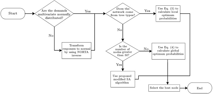
According to what has been stated so far, the proposed method is depicted in Figure 1 as a flowchart. As can be seen, either tree or general networks with normal or non-normal distributed demands can be studied with this method. In the case of general networks with a large number of nodes (greater than 50), the proposed modified SA algorithm can be used.

Figure 1. Flowchart of the proposed method.

4. Numerical examples

In all of the following examples, it is supposed that each node demand has a normal distribution with a mean of 1 and a variance of 1/12, and the fixed construction cost is equal to 10 for all nodes. In the third example, the mean and variance of each node differs from the others. Note that variance must be smaller than a third of the mean, so that negative values for demands can be negligible. Moreover, the demand of each city can affect other cities demands. To interpret this effect, we define the correlation between nodes. So, there is a correlation coefficient between each two nodes’ demands. For better comprehension of the method for solving the problems with other distributions, except that normal, we consider example 3 with another scenario in which each node has exponential distribution with a mean of 1/3. Note that Examples 2 and 4 are taken from Drezner and Shiode  [18] and the results can be compared with that paper. All examples were run on a notebook with an AMD E-350 dual-core processor and 4 GB of RAM.

4.1. Example 1

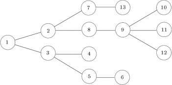
For the first example, suppose that there is a tree graph with 13 cities and 12 paths between them. Figure 2 shows the graph. It is supposed that the correlation coefficients between demands are the same and equal 0.1 for each two nodes. An algorithm was coded in MATLAB that checks all nodes and computes probabilities. The elapsed time for running the algorithm was 0.2684 of a second.

Figure 2. The tree graph with 13 nodes in Example 1.

Table 3 shows the results and it can be seen that node 2 is the best node with a probability of 0.9966.

Table 3. Probabilities results for tree network with 13 nodes in Example 1.

Node	Local optimum probability
2	0.9966
1	0.0017
8	0.0017

4.2. Example 2

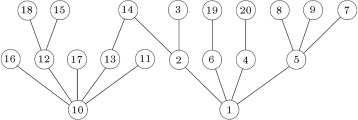
As the second example, suppose that a tree graph has 20 cities with 19 paths between them and the correlation coefficients are equal to 0.1. The tree has been shown in Figure 3 . After 0.5246 of a second, as computational time for the algorithm, it shows that node 2 is the most probable, with a probability of 0.8937.

Figure 3. The tree graph with 20 nodes in Example 2.

Table 4 shows the probabilities for some other nodes. It can be seen that the local optimum probabilities are the same as Drezner and Shiode  [18] and it confirms the accuracy of the method. It is obvious that in such problems, with few numbers of nodes, the SA algorithm cannot help reduce calculation time.

Table 4. Probabilities results for tree network with 13 nodes in Example 2.

Node	Local optimum probability	Drezner and Shiode  [18] probability
2	0.8937	0.8937
1	0.0531	0.0531
14	0.0523	0.0523
13	0.0009	0.0009

Now, let us consider some general networks. In these problems, unlike previous examples, the global optimum probability should be calculated for each node. To exemplify the proposed model, the third and fourth examples have been illustrated. However, other examples show the proposed solution algorithm performance.

4.3. Example 3

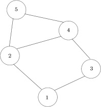
Consider a general network with 5 cities that has been shown in Figure 4 . Construction cost, ${\textstyle c}$ , matrix, mean, ${\textstyle m}$ , variance, ${\textstyle v}$ , and correlation coefficient, ${\textstyle r}$ , matrices for demands are as follows:

$c=[{\begin{array}{ccccc}10.1&10.2&11.5&10.6&10.3\end{array}}]{\mbox{,}}$

To solve this example, the algorithm takes 1.23 s. Table 5 shows the global optimum probabilities for the nodes.

Figure 4. The general graph with 5 nodes in Example 3.

Table 5. Probabilities results for general network with 5 nodes in Example 3.

Node	Global optimum probability
2	0.7433
4	0.2105
1	0.0457
5	0.0004
3	0.0000

Now, suppose that the demands have another multivariate distribution rather than normal. To study such a problem, we first use the NORTA method to transform the mentioned normal demands to exponential distributed ones. Note that the NORTA method was used to ensure correct distribution for demands. Now, suppose that all demand nodes have an exponential distribution with a mean of 1/3 and a variance of 1/9. Construction cost, ${\textstyle c}$ , and correlation coefficient, ${\textstyle r}$ , matrices have been estimated using NORTA as below:

$c=[{\begin{array}{ccccc}10.1&10.2&11.5&10.6&10.3\end{array}}]{\mbox{,}}$

By utilization of the NORTA inverse, as explained before, we can transform demands to normal distribution and then continue with the proposed method. So, after transformation demand nodes distribution to normal with a mean of 1 and standard deviation of 1/12, the correlation coefficient matrix, ${\textstyle r^{'}}$ , is, as below, for normal distributions:

$r^{'}=[{\begin{array}{ccccc}1&0.30&0.19&-0.15&0.10\\0.30&1&-0.03&0.06&0.02\\0.19&-0.03&1&0.35&0.45\\-0.15&0.06&0.35&1&0.23\\0.10&0.02&0.45&0.23&1\end{array}}]{\mbox{.}}$

Our algorithm finds node 1 as the global optimum after 2.66 s. Table 6 shows the results for other nodes:

Table 6.

Probabilities results for general network include 5 nodes with exponential demand distributions in Example 3.

Node	Global optimum probability
1	0.3849
4	0.2791
2	0.1913
5	0.1446
3	0.0001

4.4. Example 4

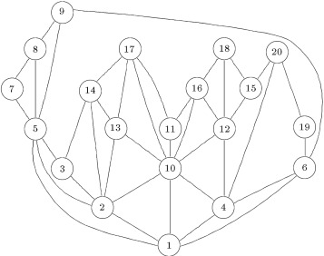
Now, suppose that we have a general network with 20 cities and 40 paths, as shown in Figure 5 . The correlation coefficients are equal to 0.3. The algorithm takes 96.99 s to answer. The results are shown in Table 7 and, as can be seen, are the same as Drezner and Shiode  [18] results.

Figure 5. The general graph with 20 nodes in Example 4.

Table 7. Probabilities results for general network with 20 nodes in Example 4.

Node	Global optimum probability	Drezner and Shiode  [18] probability
10	0.8490	0.8490
1	0.1414	0.1414
2	0.0092	0.0092
4	0.0003	0.0003

In this example, we should calculate a multivariate normal probability in a dimensionality of 19 for each node to find the global optimum probabilities. So, let us evaluate multivariate probabilities. To do it, based on the suggestion of Drezner and Shiode  [18] , for each node, ${\textstyle k}$ , first, all right hand side (RHS) values must be computed:

$RHS_{kj}={\frac {-\mu _{j}}{\sqrt {V\,ar(Y_{k}-Y_{j})}}}{\mbox{.}}$

( 9)

Now, we should determine the error rate, which is negligible for us. For this example, with an error rate of 0.0025%, the upper and lower bounds can be calculated by ${\textstyle \mu \pm \sigma Z_{\alpha /2}}$ and are 4 and −4, respectively. Then, if there is at least one RHS value smaller than lower bound, the result of multivariate normal probability can be evaluated as zero. Otherwise, a maximum of 10 largest RHS values that are smaller than upper bound must be considered, and, so, a multivariate normal probability with maximum dimension of 10 can be calculated for each node. Now, with this strategy, the algorithm running time is reduced from 96.99 to just 1.8 s. The results after evaluating multivariate normal probability are shown in Table 8 .

Table 8. Probabilities results for general network with 20 nodes by considering candidate nodes in Example 4.

Node	Global optimum probability	Number of candidate RHS values
10	0.8490	4
1	0.1414	4
2	0.0092	5
4	0.0003	5

The forth column shows the number of RHS values between −4 and 4 for each node. Note that because of less calculation, we consider up to 10 RHS values for evaluating multivariate normal distribution for each node.

4.5. Example 5

Suppose that we have a network with 100 cities and 420 paths between them, and correlation coefficients equal to 0.1. Due to the large number of nodes, it is not possible to find the global optimum probability for each node in a reasonable time, as it is necessary to calculate a multivariate normal distribution for each node with a dimensionality of 99. So, the normal distribution probability must be evaluated. Moreover, checking all nodes can require much computational time, so, an SA algorithm was coded in MATLAB. First, we try to find the best node in the same way as the previous examples. After 814.5432 s as the algorithm running time, it shows that node 3 is optimal with probability of 0.6748. Table 8 shows the results for some other nodes. Then, we use our SA algorithm to find the most probable node with default SA stopping criterion only. Computations take 679.1529 s and the result shows that node 3 is the global optimum in this network with a probability of 0.6748. By considering our proposed stopping criterion, computational time is reduced to 14.1905 s and node 3 is selected as the best node with an optimality probability of 0.6748.

Table 9 shows results for some other nodes. The fourth column shows the number of RHS values between −4 and 4 for each node. Note that because of decreasing calculation time, we consider up to 10 RHS values for evaluating multivariate normal distribution for each node.

Table 9. Probabilities results for general network with 100 nodes by considering candidates nodes in Example 5.

Node	Global optimum probability	Number of candidates RHS values
3	0.6748	5
23	0.2442	7
27	0.0254	11
56	0	13
69	0.0541	6

4.6. Example 6

Suppose a network with 50 nodes as cities and 112 links as paths. Correlation coefficients, the same as the previous example, are equal to 0.1. The proposed SA algorithm was performed for this example and after 46.5612 s, it is found that node 2 is the global optimum with a probability of 0.3310.

4.7. Example 7

Consider a graph with 150 cities and 100 paths. Correlation coefficients are equal to 0.3. To better comprehend the effect of the used trick in the SA algorithm, we perform it multiple times with different options on Example 7. At the first run, the classic framework of SA was used without any changes. The problem was solved in 1302.7548 s and the results show that node 22 is the global optimum. Then, short term memory was added to the algorithm and the computation time was reduced to 724.4957 s. It can be a great save by about 45%. At the next step, we consider the sum of distances in selecting the neighbour node. By doing this, computatinal time decreased to 365.6470 s. Finally, by adding the proposed stopping criterion, the problem is solved in about 45.6111 s only. Note that when the proposed stopping criterion is added to the algorithm, because of its excellent effect on reducing computational time, the efficiency of the short term memory and consideration of the sum of the distances can be negligible.

Table 10 shows the results of the last three examples in each method. The used method column illustrates that we checked all nodes of graph (CA), or used the Tabu search algorithm with the proposed stopping criterion (TSP), or used the proposed simulated annealing algorithm without short term memory with default stop criterion only (SA), or used the proposed modified Simulated Annealing Algorithm (SAP). Comparisons between the 3 methods show the efficiency of the proposed algorithm.

Table 10. Comparing methods in some of examples.

Example number	Best node	Optimality probability	Computational time	Used method
5	3	0.6746	814.5432	CA
5	3	0.6746	679.1529	SA
5	3	0.6749	222.9713	TSP
5	3	0.6746	14.1905	SAP
6	2	0.3310	230.4531	CA
6	2	0.3310	119.7761	SA
6	2	0.3310	122.0363	TSP
6	2	0.3310	46.5612	SAP
7	22	0.6230	3364.3945	CA
7	22	0.6229	1590.2928	TSP
7	22	0.6230	1302.7548	SA
7	22	0.6230	45.6111	SAP

As can be seen, the proposed modified SA algorithm (SAP) has the best results in all three examples in comparison with other methods.

5. Sensitivity analysis

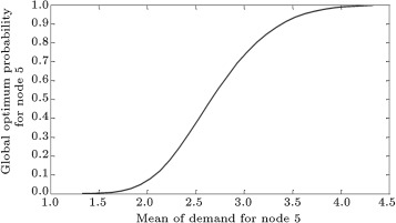
In this section, some parameters have been analyzed in the optimality probability value. Consider the third example, which is for general networks. There are 5 cities with different demand parameters. It is obvious that if a demand mean of a city increases, its optimality probability will increase. For example, if the mean of the demand for node 5 increases to 3.33, and its global optimum probability will increase from 0.0004 to 0.8825. Figure 6 shows global optimum probability changes for node 5, when it’s mean of demand increases from 1.33 to 4.33.

Figure 6. Global optimum probability changes with different value of mean of node 5 demand in Example 3.

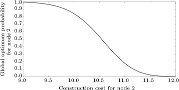
By increasing fixed construction cost on each node, its optimality probability will decrease. For example, if the fixed construction cost for node 2 increases from 10.2 to 11, its optimality probability will decrease from 0.7433 to 0.1790. Figure 7 illustrates it more clearly.

Figure 7. Global optimum probability changes according to the different values of node 2 construction cost in Example 3.

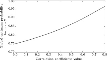
For analyzing the effect of correlation coefficients on the most probable node, suppose that all nodes have the same correlation coefficient. Figure 8 shows the global optimum probability changes for the most probable node, when correlation coefficients are the same and increase from 0 to 0.8. It can be seen that by increasing correlation coefficients, the global optimum probability for most probable node will increase.

Figure 8. Global optimum probability changes according to the node 2 correlation coefficient changes in Example 3.

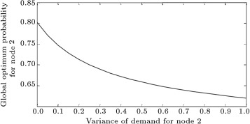
Changing the variance of the most probable node has an effect on its optimality probability, which has been illustrated in Figure 9 . It is obvious that by increasing the variance, optimality probability decreases.

Figure 9. Global optimum probability plot with different values of node 2 demand variance in Example 3.

6. Conclusions

We discussed a Weber location problem on a network with normal distributed demand points and fixed construction cost, where demands are correlated. A transformation, based on the NORTA inverse, was proposed to solve the problems with other distributions rather than normal. In a small network, we should calculate a multivariate normal distribution for each node to find the global optimum point with the most probability of optimality, but, when the number of nodes increases, finding the probability for each node needs much computational time. In this study, we proposed the SA algorithm for the stochastic one median problem. To save more time, some tricks were added to the simulated annealing. The results show that for large networks with several nodes, the proposed modified SA algorithm is an efficient solution approach. Two-median and generally ${\textstyle p}$ -median location problems can be studied in the future. Also, location-allocation problems with normal distributed demand points can be studied, as other related future research.

References

1. [1] S. Hakimi; Optimum location of switching centers and the absolute centers and medians of a graph; Operations Research, 12 (1964), pp. 450–459
2. [2] H. Frank; Optimum locations on graphs with correlated normal demands; Operations Research, 15 (1966), pp. 552–557
3. [3] H. Frank; A note on a graph theoretic game of Hakimi’s; Operations Research, 15 (1967), pp. 567–570
4. [4] H. Frank; Optimum location on a graph with probabilistic demands; Operations Research, 14 (1966), pp. 409–421
5. [5] G.O. Wesolowsky; Probabilistic weights in the onedimensional facility location problem; Management Science, 24 (1977), pp. 224–229
6. [6] Z. Drezner, G.O. Wesolowsky; The expected value of perfect information in facility location; Operations Research, 28 (1980), pp. 395–402
7. [7] Z. Drezner, G.O. Wesolowsky; Optimum location probabilities in the lp distance Weber problem; Transportation Science, 15 (1981), pp. 85–97
8. [8] O. Kariv, S. Hakimi; An algorithmic approach to network location problems II: the ${\textstyle p}$ -medians  ; SIMA Journal of Applied Mathematics, 37 (1979), pp. 539–560
9. [9] O. Berman, J. Wang; The 1-median and 1-antimedian problems with continuous probabilistic demand weights; INFOR, 44 (2006), pp. 267–283
10. [10] O. Berman, J. Wang; The network ${\textstyle p}$ -median problem with discrete probabilistic demand weights  ; Computers & Operations Research, 37 (2010), pp. 1455–1463
11. [11] O. Berman, Z. Drezner; The ${\textstyle p}$ -median problem under uncertainty  ; European Journal of Operational Research, 189 (1) (2008), pp. 19–30
12. [12] R. Tadei, N. Ricciardi, G. Perboli; The stochastic ${\textstyle p}$ -median problem with unknown cost probability distribution  ; Operations Research Letters, 37 (2) (2009), pp. 135–141
13. [13] O. Berman, D. Krass; On ${\textstyle n}$ -facility median problem with facilities subject to failure facing uniform demand  ; Discrete Applied Mathematics, 159 (6) (2011), pp. 420–432
14. [14] O. Berman, D. Krass, J. Wang; The probabilistic gradual covering location problem on a network with discrete random demand weights; Computers & Operations Research, 38 (11) (2011), pp. 1493–1500
15. [15] X. Li, Y. Ouyang; A continuum approximation approach to reliable facility location design under correlated probabilistic disruptions; Transportation Research Part B: Methodological, 44 (4) (2010), pp. 535–548
16. [16] M. Albareda-Sambola, E. Fernández, F. Saldanha-da-Gama; The facility location problem with Bernoulli demands; Omega, 39 (3) (2011), pp. 335–345
17. [17] I. Averbakh; Complexity of robust single facility location problems on networks with uncertain edge lengths; Discrete Applied Mathematics, 127 (3) (2003), pp. 505–522
18. [18] Z. Drezner, S. Shiode; A distribution map for the one-median location problem on a network; European Journal of Operational Research, 179 (2007), pp. 1266–1273
19. [19] T. Drezner, Z. Drezner; The Weber location problem: the threshold objective; Information Systems and Operational Research, 49 (2011), pp. 212–220
20. [20] S.T.A. Niaki, B. Abbasi; Monitoring multi-attribute processes based on NORTA inverse transformed vectors; Communications in Statistics–Theory and Methods, 38 (2009), pp. 964–979
21. [21] Cario, M.C. and Nelson, B.L. “Modeling and generating random vectors with arbitrary marginal distributions and correlation matrix”, Department of Industrial Engineering and Management Sciences, Northwestern University Technical Report (1997).