Advanced computationally efficient modeling of RC structures nonlinear cyclic behavior

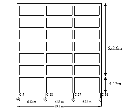
“Structural engineering is the art of molding materials we don't wholly understand, into shapes we can't fully analyze, so as to withstand forces we can't really assess, in such a way that the community at large has no reason to suspect the extent of our ignorance”

James E. Amrhein

Resumen

El comportamiento estructural de edificios y otras construcciones bajo severas excitaciones sísmicas es muy complejo e implica temas como, la interacción suelo-estructura, grandes esfuerzos y desplazamientos, daños, plasticidad y el comportamiento de la estructura cerca del colapso. Por otra parte, en estructuras de hormigón armado, existen varios modos de fallo y de degradación: agrietamiento, aplastamiento y desprendimiento del hormigón, plastificación y extracción de las armaduras traccionadas y plastificación y pandeo de las armaduras comprimidas. Además, otras circunstancias hacen que la situación sea más alarmante: dada la creciente conciencia y preocupación por el enorme riesgo sísmico mundial, la ingeniería sísmica ha experimentado en los últimos años avances sustanciales, para lo cual se han propuesto nuevas estrategias de análisis y diseño, lo que conduce a desarrollos relevantes. Estos desarrollos se basan en pruebas y simulaciones numéricas basadas principalmente en modelos simplificados referidos en este trabajo como modelo basados en la estructura, resultando un costo computacional moderado. Por lo tanto, existen una gran necesidad de verificar la fiabilidad de los nuevos desarrollos en comparación con los análisis realizados utilizando herramientas de simulación más avanzadas y con ensayos. Esta trabajo se organiza en dos partes; en la primera se describe un modelo preciso basado en la mecánica del medio continuo y en la segunda se presenta otro modelo más simplificado basado en los componentes de la estructura.

Primera parte. En esta parte se desarrolla un nuevo modelo basado en la mecánica del medio continuo para simular el comportamiento monotónico y cíclico de estructuras de hormigón armado. El modelo desarrollado combina una nueva metodología para el cálculo de las variables del daño en el Modelo de Daño Plástico del Hormigón “CPDM”, y un nuevo enfoque para integrar el CPDM con un modelo de interface de 3-D desarrollado en otra investigación. También se presenta un nuevo esquema para implementar la interfaz del modelo en un modelo FEM continuo de regiones con armaduras que se cruzan en varias direcciones. La precisión, la fiabilidad y la insensibilidad a la malla del modelo propuesto se verifican simulando varias pruebas incrementales y cíclicas; los resultados obtenidos se comparan con experimentales, lográndose un ajuste satisfactorio.

Segunda parte. El modelo desarrollado en el Primer Parte ha sido comparado con modelos simplificados basados en los componentes estructurales de uso común en la ingeniería sísmica, los resultados mostraron la superioridad del modelo propuesto para predecir el comportamiento real de los elementos y pórticos RC altamente dañados, capturando la reducción de la resistencia, la degradación de la rigidez y el efecto pinzamiento (“pinching”). Sin embargo, algunos de los modelos basados en componentes estructurales han mostrado un desempeño aceptable teniendo en cuenta el costo computacional de la ley en comparación con el modelo avanzado basado en la mecánica del medio continuo. Con de esta conclusión, este parte de este trabajo presenta un estudio numérico sobre la relación entre los modos de deterioro no-simulados de pórticos de hormigón sin ductilidad y su capacidad última. Se ha desarrollado un modelo avanzado basado en los componentes de la estructura para simular el comportamiento dinámico no lineal de las estructuras sin ductilidad, teniendo en cuenta los modos de deterioro de flexión, corte y axial. El modelo desarrollado es numéricamente eficiente, siendo pues adecuado para el uso profesional en ingeniería sísmica. La capacidad del modelo desarrollado se verifica mediante la simulación del comportamiento dinámico no lineal de un edificio no dúctil existente y del edificio prototipo. Los resultados obtenidos muestran que el desarrollado, a pesar de su coste computacional moderado, detecta y reproduce con precisión el comportamiento dinámico no lineal de estructuras RC no dúctiles, capturando también los modos de deterioro que no contemplan los modelos más simplificados. La comparación con los resultados de modelos más simplificados resalta la importancia de los modos de falla no considerados en el comportamiento de cada elemento y en los mecanismos generales de colapso. Se aborda la relación entre los modos de fallo no simulados y el fenómeno de la “Resurrección Estructural”.

Summary

Under severe seismic excitation, structural behavior of buildings and other constructions is highly complex. It involves, among other issues, soil-structure interaction, large strains and displacements, damage, plasticity, and near-collapse behavior. Moreover, in reinforced concrete structures, there are several coupled degradation and failure modes: cracking, crushing and spalling of concrete, yielding and pull-out of tensioned reinforcement, yielding and buckling of compressed reinforcement. Furthermore, another circumstance makes the situation more alarming: given the increasing awareness and concern on the huge worldwide seismic risk, earthquake engineering has experienced in last years substantial advances. New design and analysis strategies have been proposed, leading to relevant developments. These developments rely on extensive testing and numerical simulation mainly based on oversimplified models referred in this work as structural component-based models, as a result of their moderate computational cost. Therefore, there is a strong need of verifying the reliability of the new developments by comparison with analyses performed using more advanced simulation tools and with experiments. This work is organized in two parts. First part presents an accurate model, while the second part deals with a more simplified model, although highly computational efficient.

First part. This research clarifies the aforementioned issues by developing a new continuum mechanics-based model for simulating the monotonic and cyclic behavior of reinforced concrete structures. The developed model combines a new methodology for calculating the damage variables in Concrete Plastic Damage Models “CPDM”, and a new approach to integrate CPDM with a 3-D interface bond-slip model developed by other researchers. A new scheme to implement the interface model in a continuum FEM model of regions with crossing reinforcement bars is also presented in this research. Mesh-insensitivity, accuracy and reliability of the proposed model are verified by simulating several monotonic and cyclic tests; the obtained results are compared with experimental ones, satisfactory agreement has been accomplished.

Second part. The developed model in the First Part is compared with oversimplified structural component-based models that are commonly used in earthquake engineering; results have shown the superiority of the proposed model to predict the actual behavior of highly damaged RC elements and frames, capturing strength reduction, stiffness degradation and pinching phenomena. However, some of the structural component-based models have shown an acceptable performance considering the law computationally cost in comparison with the advanced continuum mechanics-based model. After this conclusion, this part presents a numerical study on the relation among the non-simulated deterioration modes of the elements in non-ductile RC frames and their final capacity. A structural component-based model has been developed for simulating the nonlinear dynamic behavior of non-ductile reinforced structures, accounting for flexure, shear and axial deterioration modes. The developed model is numerically efficient, thus being suitable for day use in earthquake engineering. The capacity of the developed model is verified by simulating the nonlinear dynamic behavior of an existing non-ductile building and the prototype building. Obtained results show that the developed model, despite its moderate computational cost, detects and reproduces accurately the nonlinear dynamic behavior of non-ductile RC structures, as well, capturing the deterioration modes that are blind to the simplified models. Comparison with results from more simplified models highlights the importance of hidden failure modes in the behavior of each element and in the overall collapse mechanisms. The relation between the non-simulated failure modes and the so-called "Structural Resurrection" is addressed.

List of symbols

Roman letters. Lower case

a_c / a_t / b_c / b_t: dimensionless coefficients in equations

b: ${\textstyle {\epsilon }_{c}^{pl}/{\epsilon }_{c}^{ch}}$ ratio

c / c₁ / c₂: cohesion / coefficients in the uniaxial tensile behavior of concrete

d / d_c / d_t: damage variable / compression damage variable / tension damage variable

b´´/d´´: are the width and depth of the confined core respectively

f / f_cm / f_tm / f_c0 / f_t0 / f_ck: stress strength / concrete compressive stress strength / concrete tensile stress strength / limit stress of linear compressive branch / limit stress of linear tensile branch / characteristic value of concrete compressive strength

f / f_b0 / f_c0 / f_cm / f_tm / f_c0 / f_t0 / f_ck/f'_c: stress strength / biaxial compressive yield strength / uniaxial compressive yield strength / concrete compressive stress strength / concrete tensile stress strength / limit stress of linear compressive branch / limit stress of linear tensile branch / characteristic value of concrete compressive strength/concrete compressive strength.

f_y / f_u: longitudinal reinforcing bars stresses yield / ultimate

f_yh / f_u: transverse reinforcing bars yield stress

g_c / g_t: compressive / tensile energies per unit volume dissipated by damage along entire deterioration process

${\textstyle {h}_{c}}$ / ${\textstyle {h}_{t}}$: weighting factors accounting for stiffness recovery

l_eq: mesh size (finite element characteristic length)

r*: stress state; for uniaxial stress r*(σ₁₁) = 1 for tension and r*(σ₁₁) = 0 for compression

s_c / s_t: coefficients accounting for stress state and stiffness recovery effects

p: hydrostatic pressure stress

q: Von Mises-equivalent effective stress

r*: stress state; for uniaxial stress r*(σ₁₁) = 1 for tension and r*(σ₁₁) = 0 for compression

s_c / s_t: coefficients accounting for stress state and stiffness recovery effects

w / w_c: crack opening / crack opening at fracture

Roman letters. Upper case

D_b: reinforcement bar diameter

E / E₀ / E_ci: modulus of deformation / undamaged modulus of deformation / tangent modulus of deformation of concrete for zero stress

E_s / E_sh: steel modulus of elasticity / slope of hardening branch

EI_flex : column effective flexural rigidity

F: loading (yield) function

G / G_ch / G_F: flow potential / crushing energy per unit area / fracture energy per unit area

H: Mohr-Coulomb yield surface function

I₁: first invariant of stress tensor

J₂ / J₃: second / third invariants of deviatoric stress tensor

K_c: ratio of second stress invariants on tensile and compressive meridians

K_deg: shear degradation stiffness (Elwood 2005 mode [1])

C_slip: Stiffness of linear slip spring

L: column height

L: mesh size for the spring bond-slip model.

M_SP: moment at spalling of concrete

F_bs : is the equitant bond force

S₁ / S₂ / S₃: relative normal displacement / longitudinalslip / transverse slip

S_peak / ${\textstyle {S}_{max}^{+}\,/\,{S}_{max}^{-}\,/{\,S}_{cum}}$: peak slip / maximum positive slip / maximum negative slip / cumulated slip

S_R:clear spacing between bar ribs

S: is the center to center spacing of the hoops

A_s´´: is the cross-sectional area of the hoop bar

A_g/A_eff: are the gross section area/ the effective shear section area.

R_c : is the pinching parameter of [124] model.

M: fourth-order tensor for anisotropic damage model

I identity tensor

Greek letters

ε / ε_c / ε_t / ε^el / ε^pl / ε_cm / ε_tm: strain / compression strain / tensile strain / elastic strain / plastic strain / strain at compressive strength / strain at tensile strength

${\textstyle {\epsilon }_{c}^{pl}}$ / ${\textstyle {\epsilon }_{t}^{pl}}$ / ${\textstyle \,{\epsilon }_{c}^{el}}$ / ${\textstyle \,{\epsilon }_{t}^{el}}$ / ${\textstyle \,{\epsilon }_{c}^{ch}}$ / ${\textstyle \,{\epsilon }_{t}^{ck}}$ / ${\textstyle {\epsilon }_{0c}^{el}}$ / ${\textstyle \,{\epsilon }_{0t}^{el}}$: strains at Figure 27; subindexes “c”, “t”, “0c” and “0t” and refer to compression, tension, undamaged compression and undamaged tension, respectively; superindexes “pl”, “el”, “ch” and “ck” and refer to plastic, elastic, crushing and cracking, respectively

ε_s / ε_y /ε_sh /ε_u: axial steel strain / yielding steel strain / hardening steel strain / ultimate steel strain

${\textstyle {\epsilon }_{c}^{ch}}$ / ${\textstyle \,{\epsilon }_{t}^{ck}}$: crushing compressive strain / cracking tensile strain

${\textstyle {\epsilon }_{c}^{pl}}$ / ${\textstyle \,{\epsilon }_{t}^{pl}}$: plastic compressive / tensile strain

ε_sh / ε_u: steel strain that corresponds to onset of hardening / ultimate strain

ε_50u /ε_50c: are the strain corresponds to 50% of concrete maximum compressive strength for unconfined and confined concrete respectively

ρ_b,s / ρ_f,s: reduction factor in bar bearing resistance accounting for steel yielding in tension / reduction factor in bar friction resistance accounting for steel yielding in tension

ρ_b,c / ρ_f,c: reduction factor in bar bearing resistance accounting for slip history / reduction factor in bar friction resistance accounts for slip history

ρ_n: reduction factor accounting for opening of splitting cracks

ρ_sh: is the transverse reinforcement ratio

ρ´´ : is the volumetric ratio of confining hoops to volume of concrete core measured to the outside of the perimeter hoops.

ϵ: eccentricity of the plastic potential surface

ϕ: friction angle

θ: Lode similarity angle

θ: is the critical crack angle (Elwood 2005 mode [1])

θ_cap: is the plastic rotation at onset of strength loss (Ibarra et al model [2])

θ_pc: is the post-capping stiffness (Ibarra et al model [2])

λ: is the energy dissipation parameter Ibarra et al model [2])

ρ: octahedral radius

σ / σ₁₁ / σ_t0 / σ_c(1) / σ_c(2) / σ_c(3): stress / first principal uniaxial stress / uniaxial tensile stress at failure / concrete compressive stress at first / second / third segment

σ^' /α' : the deviatoric parts of the stress and backstress tensors σ /α respectively

σ₀ : the effective stresses tensor

ε/ ε^e/ ε^pl: are tensors of (total strain, elastic strain, plastic strain)

${\textstyle {\overline {{\sigma }_{c}}}}$ / ${\textstyle {\overline {{\sigma }_{t}}}}$ : effective compressive / tensile cohesion stress

σ₁:normal bond stress

σ / σ₁₁: normal stress / first principal uniaxial stress

τ₂ / τ_max / τ_b/ τ_f:longitudinalshear bond stress / peak bond strength / due to bar bearing resistance/ due to friction resistance

τ₃:transverseshear bond stress

ξ: distance from origin of stress space to stress plan

ѱ: dilatancy angle

${\textstyle {C}_{m\,}and\,{\gamma }_{m\,}}$: Steel material parameters

Φ_y: Yield curvature

Δ_y/Δ_flex/Δ_slip/Δ_shear: are the yield drift displacement/ displacement due to flexure/ displacement due to slip/ displacement due to shear.

Δ_y/L, Δ_y/L: Are the drift limit angle at flexure-shear and flexure-shear-axial deterioration (Elwood 2005 mode [1])

General introduction to earthquake engineering

This section presents a brief introduction and a concise historical review of earthquake-resistant design of structures and the nonlinear analysis of RC structures.

The first seismic analysis methods appear on the year 1923 in Japan (after the earthquake in Kanto [3] and can be included within the package of so-called Earthquake Analysis Methods Based on Resistance. These procedures were intended to provide buildings with lateral (horizontal) resistance; it was believed that if the structure of the building had enough lateral resistance it should be capable to survive the design earthquake. This resistance is guaranteed by designing the structure to be able to withstand horizontal forces applied at each floor level and in each direction of the building (usually two orthogonal directions). Figure 1 illustrates this concept.

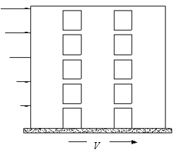
Figure 1. Lateral forces that are equivalent to a seismic input.

In Figure 1, V is the sum of the forces acting at each floor level; in other words, the horizontal interaction force between the ground and the building. V is also known as base shear. Obviously, the value of V quantifies the severity of the earthquake effect on the building.

In the firstly developed earthquake-resistant design methods, horizontal forces represented in Figure 1 were obtained by multiplying the weight of each floor by a constant coefficient. This ratio between the horizontal and vertical forces was called seismic coefficient and in the first 1923 Japanese Seismic Code [3] it was estimated as 0.1. This value gradually increased as it was experienced that structures designed with this resistance value failed when an earthquake stronger than expected occurred. This ratio took to the values of 0.10, 0.15 and 0.20 until, thanks to the development of computers and by having more and more seismic experiences, it was concluded that structures that had been designed with a certain lateral resistance, did not reach collapse but could suffer damage in the case of a larger earthquake. After that, resistance was not the primary goal and everybody started paying more attention to the ductility; it can be roughly defined as the ability of a given structure to resist after the onset of damage. The ductility of a given building can be estimated from observed damages. The regulations began to introduce the concept of ductility by quantifying it with a response reduction factor, which reduces the equivalent lateral forces shown in Figure 1; it was mentioned in the 1957 American design code [4]. Thus, this approach has been incorporated to the current worldwide regulations. In summary, most of the earthquake-resistant regulations require to provide buildings with a certain level of lateral resistance. This resistance is obtained by dividing the resistance that a given building should have to remain in the elastic range under the design input by the aforementioned response reduction factor. This factor should obviously be equal to or greater than the unity. This coefficient is represented by different symbols in each standard; in the European standard [5] it is named q, in the United States [6]it is known as R. It is remarkable that, in fact, this ratio does not take into account only the ductile behavior of the structure but also includes the over-resistance of the building due to the conservative considerations that are regularly considered (safety factors, among others) and the increase of the material resistance under dynamic inputs (“strain rate effect”).

In any case, it should be kept in mind that in these methods the effect of the earthquake on the structure is characterized by means of equivalent static forces Figure 1; they are determined as those that generate a lateral displacement equal to the maximum one that would occur along the duration of the earthquake. However, another possible strategy is to represent the seismic action by a much more direct way: as input accelerograms. In this case, dynamic analysis must be performed to determine the time-history responses; then, the maximum values will be selected, they would represent the design demands. This formulation is often referred to as earthquake-resistant design based on dynamic calculations. This strategy seems appropriate and has apparently shown to be quite capable of simulating the actual seismic behavior of structures with great accuracy and reliability; however, there are some drawbacks that hinder the use of such formulations: (1) the information about the earthquakes that may occur for a particular structure during its lifetime is limited, which severely impairs the accuracy of the study, (2) for economic reasons, structures are designed to behave nonlinearly during the design earthquake (the most severe earthquake expected with a reasonable probability) and, hence, nonlinear dynamic analyses are a must. Dynamic analyses in the nonlinear regime are much more complex than the, already complex, dynamic linear calculations.

Earthquake-resistant design based on spectra:

In general terms, these methods are based on estimating the equivalent static forces (which characterize the effect of the seismic action) in terms of the fundamental period of the structure. This is done by using response spectra; they are plots whose ordinates are certain response magnitudes and whose abscissas are the natural periods of SDOF systems that represent the structure. Up to date, three types of spectra have been basically proposed: absolute acceleration, relative displacement, and energy spectra. In the absolute acceleration spectra, the ordinates are the ratio between the maximum absolute acceleration in the top of the building and the maximum input acceleration in the base of the building. In the relative displacement spectra, the ordinates are the ratio between the maximum relative displacement between the top and the base of the building and the maximum input relative displacement. In the energy spectra, the ordinates are the input energy introduced by the seismic input in the building. It is noteworthy that each of these three spectra considers a meaningful response magnitude: the relative displacement is an indicator of the apparent structural damage level (i.e. not cumulative), the absolute acceleration is related the human perception of the motion and the damage to the facilities (and, more generally, to all the non-structural elements) and the energy reports on the accumulated structural damage.

Linear spectra plot the ratio between the maximum values of the response of an elastic single-degree-of-freedom system and of the input acceleration. Figure 2 shows an elastic model of a single-degree-of freedom system undergoing a horizontal ground motion z_g.

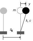
Figure 2. Elastic single-degree-of-freedom systems.

In Figure 2, m, c and k are the mass, damping and stiffness coefficients, respectively, y is the relative displacement between the mass and the base (degree-of-freedom) and z_g is the displacement of the ground. Noticeably that the model in Figure 2 can incorporate the relative displacement between the foundation and soil, this is termed as Soil Structure Interaction SSI . Yet this formulation is commonly applied to horizontal motion, can be also considered for vertical vibrations.

The equation of motion of the system described in Figure 2, is given by

$m{\ddot {y}}+c{\overset {\cdot }{y}}+ky=-m{\ddot {z}}_{g}$

(1)

By dividing both sides by m, (1) becomes

${\ddot {y}}+2z{w}_{0}{\overset {\cdot }{y}}+{w}_{0}^{2}y=-{\ddot {z}}_{g}$

(2)

In this relationship, ${\textstyle {w}_{0}}$ is the undamped natural frequency of the system and ζ is the critical damping factor. These coefficients are given by

${w}_{0}={\sqrt {\frac {k}{m}}}$ $z={\frac {c}{2m{w}_{0}}}$

(3)

The damped natural frequency ${\textstyle {w}_{d}}$ is related to ${\textstyle {w}_{0}}$ and to ζ by

${w}_{d}={w}_{0}{\sqrt {1-{z}^{2}}}$

(4)

It is remarkable that, unless the damping ζ takes extremely high values, ${\textstyle {w}_{0}}$ and ${\textstyle {w}_{d}}$ are nearly coincident.

The acceleration, velocity and displacement spectra are obtained, for each input z_g(t), as the maximum values of the absolute acceleration ${\textstyle \,{\ddot {x}}\,}$ (where ${\textstyle {\ddot {x}}=}$${\ddot {y}}+{\ddot {z}}_{g}$), relative velocity ${\textstyle {\overset {\cdot }{y}}\,}$ and relative displacement y. They depend on the natural period T (T = 2 π/ ω₀) and on the damping factor ζ. These quantities are obtained by the following linear relationships [7]:

$y\left(t\right)=-{\frac {1}{m{w}_{d}}}\int _{0}^{t}m{\ddot {z}}_{g}\left(t\right)\mathrm {sin} \,\left({w}_{d}\left(t-t\right)\right){e}^{-z{w}_{0}\left(t-t\right)}dt$	(5)
${\overset {\cdot }{y}}\left(t\right)=\int _{0}^{t}{\ddot {z}}_{g}\left(t\right)\mathrm {cos} \,\left({w}_{d}\left(t-t\right)\right){e}^{-z{w}_{0}\left(t-t\right)}dt-$${\frac {z{w}_{0}}{{w}_{d}}}\int _{0}^{t}{\ddot {z}}_{g}\left(t\right)\mathrm {sin} \,\left({w}_{d}\left(t-t\right)\right){e}^{-z{w}_{0}\left(t-t\right)}dt$	(6)
${\ddot {x}}\left(t\right)=\mathrm {\left({\frac {2{z}^{2}{w}_{0}^{2}}{{w}_{d}}}-{\frac {{w}_{0}^{2}}{{w}_{d}}}\right)\int _{0}^{t}{\ddot {z}}_{g}cos} \,\left({w}_{d}\left(t-t\right)\right){e}^{-z{w}_{0}\left(t-t\right)}dt-$$2z{w}_{0}\int _{0}^{t}{\ddot {z}}_{g}\left(t\right)\mathrm {cos} \,\left({w}_{d}\left(t-t\right)\right){e}^{-z{w}_{0}\left(t-t\right)}dt$	(7)

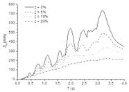
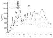
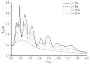
Figure 3.a.b.c show, relative displacement, relative velocity and absolute acceleration spectra, respectively. Such spectra correspond to the accelerogram registered in the ICA2 station (E-W component) during the Pisco earthquake, 15 august 2007.

1) Relative displacement spectra	2) Relative velocity spectra	3) Absolute acceleration spectra
Figure 3. Displacement, velocity and acceleration spectra for Pisco earthquake 2007- ICA2-EW

Figure 3.a.b.c show that the spectral ordinates decrease with the increasing damping ratio; this shows that damping has a beneficial effect, since it contributes to reduce relevant response magnitudes (relative displacement, relative velocity and absolute acceleration). Moreover, the spectrum corresponding to zero damping exhibits sharper peaks than the spectra for non-zero damping; it means damping contributes to smoothen the spectra, e.g. making it less sensitive to small period changes.

It has been demonstrated [8] that for small values ​​of damping and not too long periods (under 10 seconds), the velocity spectra are obtained by multiplying the acceleration spectra by T / 2π and that the displacement spectra are obtained in the same way from the velocity ones:

${\textstyle S_{v}=S_{a}(T/2\pi )</sub>\qquad S_{d}=S_{v}(T/2\pi )=S_{a}(T/2\pi )^{2}}$ (8)

Absolute acceleration response spectra

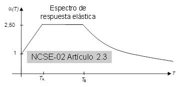
As discussed in the previous subsection, the absolute acceleration response spectra are curves that represent, in ordinates, the ratio between the maximum values of the absolute acceleration of the SDOF system that represents the dynamic behavior of the structure in a given vibration mode and the ground acceleration. The design spectra are smoothed envelopes obtained from a number of individual records. Figure 4 shows the design spectrum of the Spanish regulation [NCSE-02 2002].

Figure 4. Design acceleration spectrum [NCSE-02 2002].

The spectrum shown in Figure 4 consists of three branches: a linearly increasing one, a constant one and a hyperbolically decreasing one. Periods T_A and T_B depend on the characteristics of the soil, being higher as it has less stiffness; in some codes, the spectral ordinate (e.g. the height of spectrum) also grows as the flexibility of the soil does. The interpretation of each of these branches in terms of the effect of the earthquake on the structure is quite clear: (1) short-period structures are very rigid and tend to behave as the surrounding soil, but its motion is amplified as its rigidity decreases, (2) in the medium period range, the ground motion reaches its highest amplification inside the building and, (3) in the long periods range, structures are flexible enough so that its stiffness is not capable of overcoming the high inertia forces. This interpretation helps us to understand the influence of the soil stiffness in T_A and T_B: for stiff soil the range of building periods whose motion is highly amplified (in between T_A and T_B) is narrow, while this range widens and encompasses higher rise buildings as the soil becomes less stiff. This spectrum is commonly presented in dimensionless form (the ordinates S_a are dimensionless).

Performance-based earthquake-resistant design

The objective of the current seismic design codes is to prepare the structure to resist the design seismic input only under ultimate limit state; in other words, the structure is intended to resist the design earthquake with an acceptable level of serious damage but without collapse (in other words, avoiding at all costs the loss of human lives). Remarkably, that approach does not include any requirement about the behavior under seismic actions with lower or higher level of severity; this contrasts with the usual strategy against other type of actions (gravity, for example) where two types of limit states (ultimate and service) are considered. This approach is broadly valid and has been used for decades but was in shortage especially after the Northridge earthquake in 1994 and Kobe in 1995; after these highly severe earthquakes it was found that some structures, even those relatively new and that had been designed with the latest seismic standards, did not collapse (and in them there were no human casualties), but the damage to buildings (both structural and non-structural) was very serious. In the Kobe earthquake, some hospitals had been so intensely reinforced that effectively its structure did not collapse but absolute accelerations in the building were so high that it damaged the installations and were unusable at the time of greatest need (a few hours after the earthquake). After these events, the earthquake engineering was directed not only to prevent loss of human lives but also to quantify, reduce and prevent the damage. Depending on the damage, we are able to accept when an earthquake occurs, different solutions can be proposed. This strategy is commonly known as “Performance Based Design”; it is mainly described in the references [9], [10], [11], [12]. These documents present different seismic design methodologies oriented to control and to quantify the level of structural damage due to seismic action and to design structures that do not exceed the corresponding level.

Based on structural and non-structural damage, the following four levels of performance (“Performance States”) are defined according to SEAOC 1995 [9]:

• Fully Operational. Uninterrupted service. Negligible structural and non-structural damage.

• Operational. Most of the activities can be resumed immediately. The structure is safe and can be inhabited. The essential activities are maintained while the non-essential ones are interrupted. Repairs are necessary to resume the non-essential activities. Slight damage.

• Life Safe. Moderate damage, the structure remains safe. Some elements or components of the building may be protected to avoid damage. The risk of loss of life is low. The building may need to be evacuated after the earthquake. The repair is possible, but can be economically unfeasible.

• Near Collapse. Severe damage, but without risk of collapse. Possible fall of non-structural elements.

More recently, another similar classification is considered according to ATC-40 [10] and FEMA 356 [12];

• Immediate Occupancy. Achieve essentially elastic behavior by limiting structural damage (e.g., yielding of steel, significant cracking of concrete, and non-structural damage.). Important services are not uninterrupted. The period of lack of functionality (“down time”) is about 14 hours.

• Damage Control. Slight structural damage. Achievable occupants’ safety. The essential activities are repairable. Moderate overall damage. The period of lack of functionality (“down time”) is about 2 or 3 weeks.

• Life Safety. Limit damage of structural and non-structural components but no collapse. No risk from falling non-structural elements. The evacuation of the occupants can be done without risk. Possibility of irreparable building.

• Collapse Prevention. Severe structural damage, with risk of collapse. Likely fall of non-structural elements. The evacuation of the occupants may involve risk. Building likely irreparable.

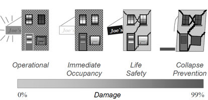
These four levels are often represented by their initials: IO, DC, LS and CP. The three levels IO, LS and CP are the most commonly used for seismic design; Figure 5 presents a graphical and easily understandable way, the practical significance of these levels and their relationship with the percentage of damage. The case “operational” in this case refers to a building without any damage.

Figure 5. Damage levels [13]

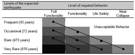
Regarding the seismic action, four levels of severity a defined as specified in Table 1.

Table 1. Severity levels of the seismic inputs

Design Earthquake	Return Periods (years)	Probability of Occurrence
Frequent	43	50% in 30 years
Occasional	72	50% in 50 years
Rare	475	10% in 50 years
Very rare	970	10% in 100 years

Table 1 shows that the severity of the earthquakes is quantified in terms of their return period; it is understood as the average of the elapsed time among earthquakes with the same magnitude or, almost equivalently, as the inverse of the probability of occurrence in one year. In some cases, seismic actions more severe than those contained in Table 1 are considered; the so-called MCE (“Maximum Considered Earthquake”) corresponds to a return period of about 2475 years. The relationship between the return period T and the probability p_n of being exceeded n years is given by the expression ${\textstyle T=}$$-n/ln\left(1-{p}_{n}\right)$ ; it is often used to indicate the severity of an earthquake by the probability p₅₀ to be exceeded in 50 years, for example, in the case of MCE

is ${\textstyle {p}_{50}=1-{e}^{-{\frac {50}{2475}}}=0.02}$ and in the case of an earthquake “Rare” is ${\textstyle {p}_{50}=1-}$${e}^{-{\frac {50}{475}}}=0.10$.

Table 2 shows the demand levels for each of the four performance levels previously described [9] , when the earthquakes that have the probability of occurrence specified in Table 1 occur.

Table 2 shows three levels of protection (expressed by the three represented diagonals): less intense for systems of moderate importance (“Basic Facilities”), more intense for major facilities (“Essential / Hazardous Facilities”) and even more intense for crucial facilities (“Safety critical Facilities”). For example, in “Essential / Hazardous Facilities” (diagonal terms) it is required that for an earthquake of return period of 75 years the building remains fully operational, for an earthquake of return period of 475 years the building keeps operating in its major functions and for a return period of 970 years the building is able to preserve the lives of its occupants.

Table 2. Severity levels of the seismic inputs and damage levels

Nonlinear static analysis (Pushover)

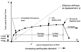
The method of earthquake-resistant design based on nonlinear static analyses consists basically of comparing the capacity of the structure, characterized by a capacity curve representing its behavior under pushing incremental forces, with the effect of the design earthquake, characterized by a demanding spectrum. The intersection between both curves is termed as target drift or target displacement or the most common “the performance point”; in other words, that point indicates the effect produced by the earthquake on the structure ATC-40 1996 [10]. The capacity curve is usually expressed by representing on the vertical axis the base shear force V and on the horizontal axis the displacement of the top floor. The analysis that generates this curve is static, monotonic, and obviously is nonlinear, being commonly known as push-over. Figure 6 shows an example of a capacity curve obtained from a push-over analysis.

Figure 6. Capacity curve obtained from push-over analyses ATC-40 1996 [10]

In the push-over analyses the base shear force is distributed along the floors according to certain patterns; the most commonly used are the first modal shape, uniform or linear (“triangular”) distributions. The push-over analyses are made incrementally, in other words, the lateral forces are increased progressively. For small values ​​of V, the behavior of the structure is linear and as V increases, the structure is becoming gradually more damaged; the stiffness of the structure decreases and its capacity curve becomes more flat. The smallest slope of the capacity curve with the increasing displacement illustrates clearly the elongation of the natural period of the structure.

Some researchers [14], [15] have proposed techniques to modify the distribution of the lateral forces among the floors to take into account the variation of the modal properties and the contribution of higher modes " Modal Push-Over Analysis".

The demand is characterized by the design spectrum for the considered level of seismic action Table 1; to be able to intersect it with the capacity curve, it is represented as the absolute acceleration spectrum S_a (vertical axis) vs. the relative displacement spectrum S_d (horizontal axis). This type of representation is commonly known as “Acceleration-Displacement Response Spectra” (ADRS).

The methods mostly used to obtain the target displacements are: Capacity Spectrum Method ATC-40 1996 [10], Displacement Coefficient Method FEMA-356 2000 [12], Equivalent linearization method FEMA-440 2005 [16], Modified displacement coefficient method FEMA-440 2005 [16], Modified Capacity Spectrum ATC-40 1996 [10].

The analysis push-over characterizes the nonlinear dynamic behavior of the structure by means of increasing static forces. The main drawback of this strategy is that the response of the structure to a given input is not incremental but cyclical and the push-over analyses cannot take into account the accumulated plastic strain, in other words, the cumulated damage. Therefore, we cannot establish a clear relationship between the maximum displacement of the structure and the energy stored during plastic deformation cycles. When the structure enters the inelastic range, deterioration occurs by the accumulation of plastic incursions; that can produce the complete breakdown of structural elements for deformations smaller than those that could be resisted under monotonic forces. This type of failure is called low cycle fatigue or plastic fatigue. Another drawback of the earthquake design strategy based on displacements is that the hysteretic behavior is interpreted as an equivalent viscous damping (ζ_eq); this introduces a relevant error, especially for significant levels of damping. Moreover, such identification is not based on any physical principle that justifies, in inelastic systems, the existence of a direct relationship between the energy corresponding to the maximum displacement and the equivalent viscous damping.

Dynamic analysis:

This procedure evaluates the effect of earthquakes on buildings based on determining the dynamic response (commonly known as “time history”) to the expected accelerograms. The most relevant response quantities are; the maximum relative displacements in between consecutive floors (inter-story drifts), and the maximum absolute accelerations. The maximum relative displacements report about the experienced level of structural damage, the maximum absolute accelerations are directly correlated with the non-structural damage and the human comfort conditions. Since the dynamic calculations take into account the performance of buildings under seismic inputs in a more direct way than in the methodologies based on response spectra, in general the dynamic analyses are able to provide more accurate results. In particular, the comparison between the nonlinear static methods (push-over) and the nonlinear dynamic methods is clearly favorable to them because, besides being more accurate in general, they have two important advantages: (i) by considering the cyclical behavior they are able to reproduce the accumulated plastic damage and (ii) the consideration of the effect of damping (both the present in the undamaged structure and the generated for increasing damage) is more direct.

In zones of medium or high seismicity, buildings are often designed by accepting a given level of structural damage under the design earthquake. Accordingly, in these cases the dynamic analyses should be nonlinear, in other words, must be able to reproduce the behavior of the structure when it been damaged and therefore has experienced significant reductions in its strength and rigidity. Moreover, second-order analyses may be necessary because of the significant relative horizontal displacements, this being another source of complexity and increased computational cost. Although the nonlinear dynamic analyses are increasingly used in the earthquake-resistant design of important structures, this procedure is rarely used in the design of ordinary structures, this is due to the high computational cost involved and to the effort required to properly interpret the large amount of generated information.

Incremental Dynamic Analysis IDA

With the main purpose of alleviating the problem derived from the fact that the push-over analysis cannot take into account the accumulated plastic strain, the so-called Incremental Dynamic Analysis IDA has been proposed [17]. It is remarkable that the incremental dynamic analyses require making several nonlinear dynamical calculations, which are expensive in computational time; on the other hand, it may be necessary to perform second-order analyses. However, the incremental dynamic analyses, especially when applied to several earthquakes, constitute powerful formulations, which may provide greater and more useful information than the rest of approaches that have been described in this section.

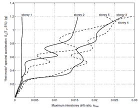
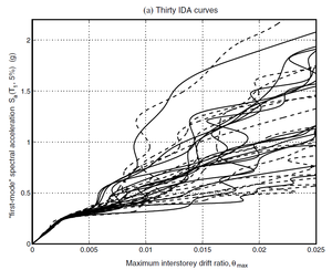
The results of these procedures are usually represented by the so-called IDA curves. These representations consist of capacity curves similar to the result of the push-over analyses; on the horizontal axis, an index related to the magnitude of the response is usually represented and the vertical axis usually contains an index related to the severity of excitation. Figure 7 shows the results of this kind; Figure 7.(a) corresponds to a single record and Figure 7.(b) corresponds to multiple (30) records. In both representations the severity of the seismic action is quantified by the ordinate of acceleration response spectrum for the first mode S_a(T₁, 0.05) and the magnitude of the response is quantified by the maximum value (along the duration of the earthquake) of the relative displacement between floors (inter-story drift). Figure 7.(a) shows both increases and decreases of the damage on the upper floors with increasing severity of excitation, this effect is obviously due to the “protection” provided by the lower floors. None of the other methods described in this section are able to predict this phenomenon so clearly. Figure 7.(b) shows the remarkable variability in the response of a determined structure to records that have, in first approximation, a comparable level of severity.

1) Single Register	2) Thirty Registers
Figure 7. Examples of IDA curves [17]

Usually the damage thresholds IO, LS and CP are related with certain values ​​of the index that quantify the magnitude of the excitation (ordinate in Figure 7); in this way performance-based analyses can be made from incremental dynamic calculations.

Deterioration modes in RC structures

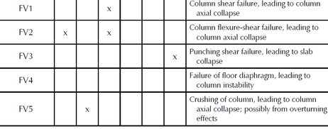
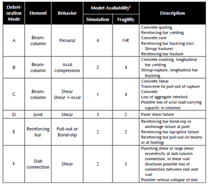
While buildings are usually designed for seismic resistance using elastic analysis, most will experience significant inelastic deformations under large earthquakes. Deterioration modes for RC frame components have been identified in [18] based on a review of experimental tests, published information and observation from past earthquakes. They are classified into six modes depending on the type of structural element and the physical behavior associated with deterioration shown in Figure 8. For each mode, currently available nonlinear components models are rated from low to high confidence “1 to 5” for their ability to simulate the deterioration.

Figure 8. Deterioration modes for reinforced concrete frame components [18]

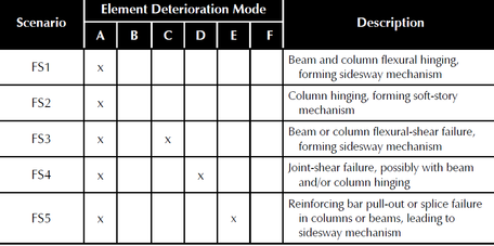
Progressive deterioration can cause structural collapse, this can be generated in two forms; Local Collapse; identified as part of structure has been collapsed in result of ground shaking causes elements deterioration modes form a collapse mechanism, the localized part in RC frame structures is one floor that is usually the so called “soft story”, vertical loads still can be transmited by the non-damaged component. Second form is the Global Collapse; the entire structure collapsed and cannot transmit any vertical neither lateral loading. In regards to structure collapse, two possible mechanisms “scenarios” are defined; Sidesway Collapse induced by dynamic instability as result of unlimited story drifts amplified by a combination of P-Δ effects and deterioration in strength of the structural components. Vertical Collapse; this kind of collapse occurs as a result of the loss of one or several elements the vertical load carrying capacity causes a local collapse, and eventually entire vertical collapse due to a developed progressive collapse mechanism. These possible collapse mechanisms are principally dependent on the developed deterioration modes at the components level. Contribution of the predefined deterioration modes on the collapse mechanism "scenario" is defined in Figure 9 according to [18].

Figure 9. Deterioration modes for reinforced concrete frame components [18]

Nonlinear Analysis

Modern performance-based design methods require ways to determine the realistic behavior of structures under strong earthquakes. Enabled by advancements in computing technologies and available test data, nonlinear analyses provide the means for calculating structural response beyond the elastic range, including strength and stiffness deterioration associated with inelastic material behavior and large displacements. As such, nonlinear analysis plays an important role in the seismic assessment of new and existing buildings. In contrast to linear elastic analysis and design methods that are well established, nonlinear inelastic analysis techniques and their application to design are still evolving and may require engineers to develop new skills. Nonlinear analyses require thinking about inelastic behavior and limit states that depend on deformations as well as forces, different degradation modes among their interaction at the structural components must to be captured.

Depending on the structural configuration, the results of nonlinear analyses can be extremely sensitive to the assumed input parameters and of implemented numerical models, these models must confirm the locations of expected or observed inelastic deformations and trace the structural behavior up to the onset of collapse. This requires sophisticated models that are validated against physical tests to capture the highly nonlinear response approaching collapse.

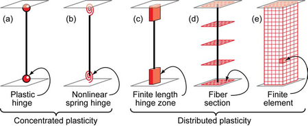
Capturing the aforementioned deterioration models and collapse mechanisms requires that the numerical model has the capacity to represent; the behavior of concrete and steel materials at high level of monotonic and cyclic loading, as well the interaction between both materials during the loading process characterized by the bond-slip behavior. Numerical models can be differentiated by the way that plasticity is distributed through the member cross sections and along its length. Figure 10 illustrates several idealized model types for simulating the nonlinear response of beam-column elements, same concepts can be applied for other element (e.g. braces and shear walls).

Figure 10. Beam-Column nonlinear models [19]

Concentrated Plasticity Models are the simplest formulation, representation of such models are shown in Figure 10-a,b. these models are based on concentrating the inelastic deformations at a specific location where the damage is expected to be located (e.g. ends of beams and columns). Numerically this is represented by attaching zero-length or spring element at location of the inelastic deformation, the behavior of this nonlinear element is governed by the so-called “backbone” or capacity curve that can be represented by moment-rotation or force-deformation relation for ductile and brittle behavior respectively. For cyclic loading, a hysteretic behavior is also incorporated in the behavior of the nonlinear element. Both the capacity curve and the hysteretic properties in these models are usually calibrated after experimental results and observation of past earthquakes. This formulation can be used to reflect the effect of some degradation phenomena such as bond-slip or bar buckling.

Distributed Plasticity Models are more complex to represent the distribution of the inelastic deformation. The distribution varies as well between the simple and the more complex. The Finite Length Hinge Model Figure 10-c is an efficient distributed plasticity formulation with designated hinge zones at the member ends. Cross sections in the inelastic hinge zones are characterized through either nonlinear moment-curvature relationships or explicit fiber-section integrations that enforce the assumption that plane sections remain plane. The inelastic hinge length may be fixed or variable, as determined from the moment-curvature characteristics of the section together with the concurrent moment gradient and axial force. Integration of deformations along the hinge length captures the spread of yielding more realistically than the concentrated hinges, while the finite hinge length facilitates calculation of hinge rotations.

Another more complex distributed plasticity formulation is the Fiber Section Model Figure 10-d. This model distributes plasticity by numerical integrations through the member cross sections and along the member length. The section is discretized by several fibers “portions”. Uniaxial material models are defined to capture the nonlinear hysteretic axial stress-strain characteristics in the cross sections, each fiber is assigned to a material (e.g. steel, confined and unconfined concrete). The plane-sections-remain-plane assumption is enforced, where uniaxial material “fibers” are numerically integrated over the cross section to obtain stress resultants (axial force and moments) and incremental moment-curvature and axial force-strain relations. The cross section parameters are then integrated numerically at discrete sections along the member length, using displacement or force interpolation functions. The most complex models are the Continuum Models Figure 10-e. These models discretize the continuum along the member length and through the cross sections into small (micro) finite elements with nonlinear hysteretic constitutive properties. This fundamental level of modeling offers the most versatility since the inelastic behavior can be captured in all the location and for different material, moreover the relation between concrete and steel “bond-slip” can be treated also by a constitutive model. The big challenge for Continuum formulation is providing integrated efficient model for RC simulation.

From the previous literature; two main modeling formulations can be defined to simulate the complex inelastic behavior of RC structures, the definition is based on the method each model presents the degradation at the components and material levels. The most commonly used formulation in earthquake engineering and performance based design is the Structural Component-Based Formulation represented by the models in Figure 10-a,b,c,d, and the most complex and general formulation is the Continuum-Based Formulation represented by Figure 10-e. In this dissertation, the simple and advanced formulations are verified and used to develop an appropriate tool for simulating the nonlinear dynamic behavior of RC frame structures.

Objectives

Main objective

To establish the requirements of developing a computationally efficient model for nonlinear cyclic behavior for RC structures. This study will consider advanced models derived from continuum mechanics-based formulations, and the simplified structural component-based models. This research will focus on RC frames behavior.

Particular objectives

This global objective will be pursued through the following particular objectives:

• Review the numerical models commonly used for describing the nonlinear dynamic behavior of RC frames under earthquake excitation. This study encompasses the most spread models based on structural component-based approaches (e.g. Lumped Plastic, Distributed Plastic).

• Review the more sophisticated numerical models derived from continuum mechanics formulations. This study encompasses the models for concrete, reinforcing bars and the models to describe the relation between both materials under monotonic and cyclic loading.

• Development of 3D continuum mechanics-based model for simulating the nonlinear cyclic behavior of RC structures, the model uses concrete plastic damage model and phenomenological interface bond-slip model.

• Verifying the capacity of the developed 3D continuum mechanics-based model, as well the simplified components-based models with experimental results of RC structures subjected to monotonic and cyclic loading.

• Development of an advanced and day use structural component-based model to simulate the nonlinear dynamic behavior of non-ductile RC structures.

• Performing Incremental Dynamic Analysis (IDA) study using the developed structural component-based model. The study investigates the importance of hidden failure modes as well as the relation between these modes and the so called “Structural Resurrection Phenomena”

Outline

This dissertation is organized in two parts, description of each part as well the new contribution is presented as follow:

Part I focuses on the "numerical models of RC structure that are based on continuum mechanics-based formulations". Two major contributions are developed in this part. First contribution is a new methodology for calculating the damage variables "damage evolution" in Concrete Plastic Damage Models (CPDM), implementation of this methodology for CPDM of ABAQUS finite element analysis program is described as well. The second contribution is a new modeling scheme for 3D implementation of an interface bond-slip model developed by [20] and implemented in ABAQUS. Combining the methodology for calculating damage evolution in CPDM, as well the modeling scheme of the bond-slip model, results in an integrated continuum-based model for monotonic and cyclic simulation of RC structure. Proposed model is implemented in ABAQUS and verified with experimental results. Part I is organized in seven chapters as follow:

Chapter 1 provides an introduction to Part I, motivation and new contribution are also described. Chapter ‎2 describes in general the modeling of concrete material, models derived from plasticity, damage and coupled plastic-damage are described in this part, as well as the used concrete plastic damage model. Chapter 3 presents the proposed methodology for calculating the damage evolution in concrete plastic damage models. Chapter 4 describes the used model of steel material, while Chapter ‎5 describes the bond-slip phenomena and the implemented interface model in this work, the new modeling scheme is described in the subsection ‎5.4. Chapter ‎6 presents numerical simulation of real experiments conducted on reinforced concrete structures, experimental results are compared with ones obtained by the proposed models, finally Chapter ‎7 addresses a general concluding remarks about Part I.

Part II focuses on numerical models that are based on simplified formulations referred as "structural component-based approaches" models. In this part the oversimplified models and commonly used in earthquake engineering are verified with experimental results and compared with the advanced model derived in Part I. The main contribution in this part is developing an advanced structural component-based model for nonlinear dynamic simulation of non-ductile RC framed structures. A numerical study is conducted using the developed model on the relation among the non-simulated deterioration modes of the elements of non-ductile RC frames and their final capacity. Part II is organized in six chapters as follow:

Chapter 1 provides an introduction to Part II, motivation and new contribution are also described. Chapter ‎2 describes the structural component-based models commonly used in the simulation of reinforced concrete structures. Chapter ‎3 verifies the capacity of the models presented in chapter ‎2 to capture the nonlinear behavior of the simulated experiments in Part I, obtained results are also compared with the ones from the continuum mechanics-based model developed in Part I. Chapter ‎4 presents the developed model to simulate the nonlinear dynamic behavior of non-ductile reinforced concrete structures. Chapter ‎5 verifies the capacity of the presented model in chapter ‎4 by performing numerical simulation of a two non-ductile structures, obtained results are also compared with experimental ones. Conclusions of this part are addressed in Chapter ‎6.

In the final conclusions chapter, the achievements of the present study are exposed along with concluding remarks and future works derived from this dissertation.

1 Introduction and motivation

Under severe seismic excitation, structural behavior of buildings and other constructions is highly complex. It involves, among other issues, soil-structure interaction, large strains and displacements, damage, plasticity, and near-collapse behavior. Moreover, in reinforced concrete structures, there are several coupled degradation and failure modes: cracking, crushing and spalling of concrete, yielding and pull-out of tensioned reinforcement, yielding and buckling of compressed reinforcement. Numerical model must be able to predict the global behavior of the elements among the interaction of the forces acting on each element. In other words, the model must capture the interaction between axial, shear, torsion and flexural moment, as well the subsequent degradation modes represented in strength reduction, stiffness degradation and pinching. Models based on simplified theories referred in this work as structural component-based models are commonly used in earthquake engineering, as a result of their moderate computational cost. Such models might serve to predict the seismic behavior of RC structures in some particular cases. However, in many cases the oversimplified models are not capable to capture adequately the entire range of deformation till the structure reaches its collapse state.

Therefore, in earthquake engineering, advanced numerical simulations based on continuum mechanics are strongly necessary. These models are commonly used in small size simulation due to their expensive computationally cost. The motivation in this part is to developed computationally efficient model based on advanced formulations. The developed model can be used for simulating small size structures or to investigate particular joints or some parts in reinforced concrete structures. Another application of the proposed model is to improve the performance of existing simplified models, as well to calibrate new models that can be used afterwards to simulate large scale models.

Using continuum mechanics-based formulations to describe the behavior of a mixed material such concrete implies that each material is assigned to a set of elements, the relation between materials must be also described by incorporating new elements or by imposing some bond conditions. In the developed model, concrete material is simulated by solid finite elements, steel bars are simulated by truss finite element and bond between steel and concrete is simulated by either; an interface elements or by assuming perfect bond conditions for cyclic and monotonic loading respectively. This part of the work describes shortly the bases of concrete constitutive modeling, as well the used damage-plastic model. Regarding steel bars, the basic plasticity model is described with its implementation. The complex relation between concrete and steel bars "bond-slip" is revised under monotonic and cyclic loading, modeling these phenomena in a 3D continuum model is explained.

The main contributions in this part are: Developing a new methodology for calculating the damage variables "damage evolution" in Concrete Plastic Damage Models "CPDM" [21] [22] [23] [24] [25] [26] [27] [28] [29] [30], this methodology is described in section ‎3. As well as a new scheme to implement interface bond-slip model in 3D FEM simulation described in subsection ‎5.4. As a final contribution, a new approach to integrate CPDM and bond-slip model in simulating the cyclic and monotonic behavior of RC structures is presented in subsection ‎6.1

2 Concrete modeling

2.1 Introduction

Quasi-brittle materials, as concrete, exhibit nonlinear stress-strain response mainly because of micro-cracking. Cracks are oriented as the stress field and generate the failure modes. In tension, failure is localized in a narrow band; stress-strain behavior is characterized by sudden softening accompanied with reduction in the unloading stiffness. In compression, failure begins usually in the outside and is more complex, involving volumetric expansion, strain localization, crushing, inclined slipping and spalling; stress-strain behavior involves ductile hardening followed by softening and reduction in the unloading stiffness. In mixed stress states, failure depends usually on the ratio between the principal stresses. Nonlinear concrete response can be represented using plasticity or damage theory. However, none of these formulations alone is able to describe adequately this phenomenon. Plastic models [31] [32] might represent realistically the observed deformation in high confined concrete but do not capture the stiffness degradation observed in experiments [21]. Damage-based models [33] [34] [35] [36] are based on gradual reduction of the elastic stiffness; they can describe the stiffness degradation in tension and low confined compression, but are not suitable to capture the irreversible deformations observed in experiments and the inelastic volumetric expansion in compression. In addition, fracture propagation can be represented by embedded crack models, where standard FEM interpolations are enriched with strain or displacement discontinuities [37] [38] [39]. These models can be used for high strain localization problems (fracture). The mechanical behavior among the constitutive modeling of concrete are described in the next sections.

2.2 Mechanical behavior

The fundamental characteristics of concrete behavior are established through experimental testing of plain concrete specimens subjected to specific, relatively simple load histories. Continuum mechanics provides a framework for developing an analytical model that describe these fundamental characteristics. Experimental data provide additional information for refinement and calibration of the analytical model. Some important mechanical features of concrete are summarized in this section. This furnishes a background for the review and further study on the constitutive modelling of concrete in the following subsections.

2.2.1 Uniaxial behavior

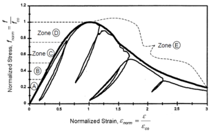
The behavior of concrete is highly nonlinear in both uniaxial tension and compression. Under uniaxial compression stress state, five different deformational stages can be observed as shown in Figure 11.a. For axial stresses up to about 30% of the maximum compressive stress, the uniaxial compressive behavior of concrete can be considered linear with existing micro-cracks in the material remaining nearly unchanged (Zone A). The second stage is between 30 % and 50% of the maximum compressive stress, results in some reduction in the initial stiffness due to the significant increase in crack imitation (Zone B). noticeably that crack does not continue to grow under constant load. Third stage is between 50 % and 75% of maximum compressive stress, results also in more reduction in the initial stiffness due to further initiation and growth of crack (Zone C). At this stage crack continue to grow under constant load. For stress state more than 75% of the maximum compressive strength, results in increasing compressive strain under constant loading (Zone D). After reaching the maximum compressive stress, softening behavior is observed with crack localization that varies according to the boundary conditions (Zone E). The softening under compression is more complicated than tension one and no general model is yet accepted such the crack model in tension. This is because of many factors such as the size and shape of the specimen, concrete strength and boundary conditions.

a) Stress-strain relation [40]	b) normalized stiffness reduction evolution versus normalized plastic strain under cyclic loading [41]
Figura 11. Uniaxial concrete response under monotonic and cyclic compression loading

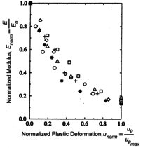
Uniaxial compression under cyclic loading shows important characteristics as shown in Figure 11.a; the developed stress follows the path of monotonic stress response, initial stiffness in each unloading and reloading stiffness faces a progressive deterioration with increasing the demand. The phenomena of stiffness degradation upon increasing the demand is referred as damage. Figure 11.b; shows a plot a data from [41] of normalized unloading stiffness as a function of normalized plastic compressive deformation. Plastic deformation is defined as the deformation that is not recovered upon unloading to zero compressive stress and this deformation is normalized with respect to the deformation at approximately zero compressive strength.

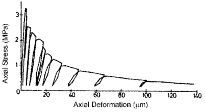
In uniaxial tension stress state, observed deformation process is different from that in compression. The low tensile strength of concrete is primarily due to the low tensile strength of the aggregate-mortar interface, which has a significantly lower strength than the mortar. This interface is known to be the weakest link in this composite material, with cracks usually occurring at the interface. Figure 12 shows typical concrete stress stain response under cyclic loading [42]. The response is essentially linear before reaching the maximum tensile strength capacity, corresponds to stable microcracks. After reaching the maximum strength, softening is observed due to the development of localized continuous crack system mainly perpendicular to the stress direction. Unloading and reloading after reaching the maximum capacity showed also degradation in the initial stiffness.

Figure 12. Uniaxial concrete response under cyclic tension loading [42]

2.2.2 Multiaxial behavior

Since plain concrete in RC elements is usually subjected to multi-dimensional stresses, developed constitutive models are not only based on the uniaxial behavior of concrete. A number of researchers have studied the biaxial and triaxial behavior of concrete experimentally and analytically.

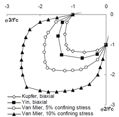
Investigations by [43] and [44] mainly focused on biaxial loading and developed experimentally a failure surface as shown in Figure 13. The 2D failure surfaces were extended by data from [45] by studying the effect of low levels of confinement pressure in the third direction. Results obtained by [45] showed that relatively small confinement pressure can significantly increase the concrete strength in the direction perpendicular to the confinement pressure up to 2.5 times the uniaxial compressive strength Figure 13.

1) Biaxial compressive failure surface for concrete. Data from [43,44,45] and presented by [46]	2) Concrete tensile and compressive meridians. Data from [47-50] and presented by [51]
Figure 13. Experimental failure surfaces for concrete

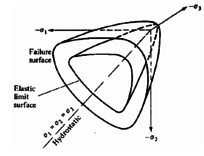
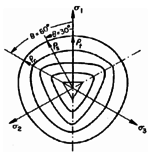
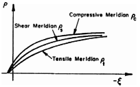
Tow envelopes must be considered to describe the behavior of concrete; elastic limit surface defining the elastic region and the failure surface characterizing the maximum-strength envelope as shown in Figure 14.a. It's been wildly accepted that concrete behavior can be considered as isotropic, therefore both surfaces can be described in terms of stress invariants; I₁ the first invariant of the stress tensor, J₂ and J₃ the second and third invariants of deviatoric stress tensor respectively. Haigh-Westergaard space can be used to define the failure surface in principal stress space Figure 14.a.b, in which the position of a stress point is determined by three coordinates ρ , ξ and θ, where ρ is the octahedral radius, ξ is the distance from the origin of stress space to the stress plan, θ is the Lode similarity angle.

${I}_{1}\,={\sigma }_{11}+{\sigma }_{22}+{\sigma }_{33}$

(9)

${J}_{2}\,={\frac {1}{6}}\left[{\left({\sigma }_{11}-{\sigma }_{22}\right)}^{2}+\right.$$\left.{\left({\sigma }_{22}-{\sigma }_{33}\right)}^{2}+{\left({\sigma }_{33}-{\sigma }_{11}\right)}^{2}\right]+$${{\sigma }_{12}}^{2}+{{\sigma }_{13}}^{2}+{{\sigma }_{23}}^{2}$

(10)

${J}_{3}\,={\frac {1}{27}}\left(2{I}_{1}^{3}-9{I}_{1}{I}_{2}+27{I}_{31}\right)$

(11)

$\xi \,={\frac {{I}_{1}}{\sqrt {3}}}\qquad \qquad$ $\rho \,={\sqrt {2{J}_{2}}}$

(12)

a) In principal stress space [52]	b) In deviatoric plans [53]	c) In the meridian sections [53]
Figure 14. Concrete failure surfaces in different views

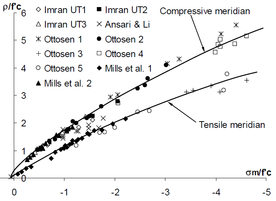
From experimental results in Figure 13, it can been seen that the failure surface has an open shape. The shapes of the failure surface in the deviatoric and meridians plans is shown respectively in Figure 14.b.c, it can be seen that the deviatoric plans are different in size and shape according to the level of the hydrostatic pressure. ρ_s, ρ_t and ρ_c correspond respectively to shear, tension and compression meridians and are determined according to Lode angle.

2.3 Concrete constitutive models

In principle, it is desired that the above-mentioned macroscopic features of the

material behavior be reflected in any constitutive models dedicated to concrete

modelling. However, it is quite difficult to incorporate all of these aspects of material

behavior in a constitutive model. Those experimentally observed features are all of

macroscopic nature, which can only be characterized through some material and

structural quantities and cannot always represent what truly happens at the microscopic

level. This is the disadvantage of the macroscopic approach to constitutive modelling. However, developing an analytical model for concrete has been the aim of many researchers in the last thirty years. Early models were based on elastic theory, more recent use plasticity, damage and fracture mechanics. Majority of the models capture particular aspects concrete response under different type of loading, however, most of the models have acceptable accuracy and efficiency.

2.3.1 Models based on plasticity

Plasticity in material can be defined as the accumulation of uncovered deformation upon loading beyond the yield limit. Experimental results showed that concrete exhibits plastic strain when it's subjected to compression and tension, therefore, constitutive model must incorporate plastic theory.

Developing a plasticity-based constitutive model requires defining; rule for decomposition of the total stain, elastic material constitutive relationship, yield/failure surfaces law and flow rule.

The total stain is usually assumed to be the sum of elastic and accumulated plastic strain

${\overset {\cdot }{\boldsymbol {\varepsilon }}}\,={\overset {\cdot }{{\boldsymbol {\varepsilon }}^{e}}}+$${\overset {\cdot }{{\boldsymbol {\varepsilon }}^{pl}}}$

(13)

Elastic constitutive relationship follows Hook's law

${\boldsymbol {\quad \quad \,\,}}{\overset {\cdot }{\boldsymbol {\sigma }}}=\,{\boldsymbol {D}}_{0}^{el}\,:{\overset {\cdot }{{\boldsymbol {\varepsilon }}^{e}}}=$${\boldsymbol {D}}_{0}^{el}\,:\left({\overset {\cdot }{\boldsymbol {\varepsilon }}}-{\overset {\cdot }{{\boldsymbol {\varepsilon }}^{pl}}}\right)$

(14)

${\textstyle {\boldsymbol {D}}_{0}^{el}}$ is the elastic stiffness tensor, ${\textstyle {\boldsymbol {\sigma }}}$ and ${\textstyle {\boldsymbol {\epsilon }}}$ are the stress and strain tensors.

For concrete, the available material data facilitated definition of the yield surface in stress space and it is most appropriate to consider a yield surface that evolves as a function of the load history. A hardening rule defines the evolution of the yield surface. The flow rules define the evolution of a set of internal variables that uniquely define the material state. In particular, a flow rule defines the orientation of plastic strain which may be associated, defined as normal to the yield surface, or non-associate. Proposed plastic models for concrete vary in the definition of the yield surface, the hardening rules and the flow rules.

Regarding the distinction of the yield surface and the failure surface Figure 14.a, we can see that these two surfaces coincide in plasticity theory. In other words, a single loading surface acts as a yield-failure surface in plasticity theory. This combined surface is often a scaled down version of the failure envelope of the material. Numerous forms of yield surfaces have been proposed and can be classified based on either the number of model parameters [53] or on the shape of the surface in principal stress space.

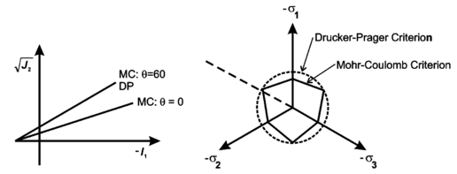
The first yield criteria to characterize the behavior of plain concrete were Mohr-Columb and Druker-Prager [42] shown in Figure 15, these criteria were developed to describe the response of material such as sand, rock and concrete for which hydrostatic pressure affects the material yield and failure strengths.

The Mohr-Coulomb criterion is defined as follows:

$H\left({I}_{1},\,{J}_{2},\theta ,\phi ,c\right)=\,{\frac {1}{3}}{I}_{1}\,sin\,\phi +$${\sqrt {\,{J}_{2}}}sin\,\left(\theta +{\frac {\pi }{3}}\right)+\,{\frac {\sqrt {\,{J}_{2}}}{\sqrt {\,3}}}cos\left(\theta +\right.$$\left.{\frac {\pi }{3}}\right)sin\phi -c\,cos\phi =0$	(15)
$\theta =\,{\frac {1}{3}}\mathrm {acos} \,\left({\frac {3{\sqrt {3}}}{2}}{\frac {\,{J}_{3}}{\,{{J}_{2}}^{\frac {3}{2}}}}\right)$	(16)

In the previous, ϕ is the friction angle, and c is the material cohesion. Equations (15) and (16) represent a straight line of variable slope in the meridian plane and an irregular hexagon in the ${\textstyle \pi }$ plane as shown in Figure 15.

Figure 15. Mohr-Coulomb and Drucker-Prager Failure Criteria [42]

The Drucker-Prager criterion represents moderately well the response of plain concrete

subjected to multi-axial compression and provides a smooth yield surface Figure 15. This criterion is defined as follows:

$H\left({I}_{1},\,{J}_{2},\alpha ,y\right)={\sqrt {\,{J}_{2}}}+\alpha {I}_{1}+y=$$0$

(17)

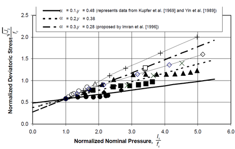
In the previous criterion, α and y are material constants. The values of theses constants significantly change the yield surface as shown in Figure 16.

Figure 16. Drucker-Prager Failure Criterion Compared with Experimental Data as presented by [51]

As indicated in Figure 16, Imran and Pantazopoulou 1996 [48] propose α =0.3 for characterizing the response of concrete subjected to triaxial compression. The response of concrete subjected to biaxial compressive loading Kupfer et al. 1969 [43] and Yin et al. 1989 [44] is characterized well by α =0.1. All of the presented yield criteria are calibrated to predict the observed uniaxial compressive strength.

Comparison of the Drucker-Prager criterion with experimental data shows that while

the criterion may be used to represent the response of concrete subjected to multi-axial

compression, the model over-estimates the capacity of concrete subjected to compression-tension or tension-tension type loading. Variation in concrete response under various load regimes has been addressed by a number of researcher through the use of multi-surface plasticity models. Murray et al. 1997 [54] model proposes a three surface model to characterize the response of plain concrete subjected to biaxial loading, this approach was extended to concrete loaded in three-dimensions by Chen and Chen 1975 [31] and Lubliner et al. 1989 [30].

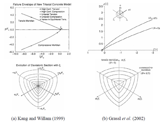
The main shortcoming of Mohr-Columb and Druker-Prager surfaces is that they assume a linear relationship between J₂ and I₁ (between ρ and ξ in the meridian plan), although this relationship has been experimentally shown to be nonlinear Figure 14.c. More recent failure criteria with nonlinear relation between J₂ and I₁ with incorporating Lode angel θ in the formulation have incorporated the [53], [55], [51], [56]. The typical deviatoric and meridian sections of those failure surfaces are shown in Figure 17

Figure 17. Deviatoric and meridian sections of two typical failure surfaces

In plasticity theory, the definition of a yield surface, the shape of which is usually similar to that of the failure surface (i.e. the yield surface by Grassl et al. 2002 [56]), is required. However, as pointed out by [53] yield surfaces as scaled down versions of failure surfaces at maximum loading are inadequate for concrete modelling. The open shape of such yield surfaces does not reflect the true behavior of concrete under hydrostatic loading. A solution for this is the use of an additional “cap surface” for the behavior of the model under hydrostatic compressive pressure.

The volumetric expansion of concrete under compression makes the application of the associated flow rule for concrete inappropriate. A non-associated flow rule, which is defined by the plastic potential other than the yield function should be used instead. This feature is included in the model developed by [53], [22], [55]. Deterioration in the initial stiffness beyond unloading and reloading has a significant impact on the response of RC structures. Such aspect should be captured by the analytical model that aims to represent the behavior under cyclic loading. Conventional plasticity models are not able to represent this degradation as plastic theory was invented for metallic materials.

2.3.2 Models based on damage mechanic

The damage "stiffness degradation" of a continuous solid is an alteration of the elastic properties during load application due to a decrease of the effective strength area. This effective area loss is normally caused by the increase of voids and/or micro fractures [57]. The continuous damage theory was first introduced by Kachanov in 1958 [58], further contribution was given by Rabotnov in 1963 [59] by introducing the concept of effective stresses. However, the basic development of continuum damage mechanics only began in the 1970s and then in the 1980s with a more rigorous basis, based on thermodynamics and micromechanics. Since then there have been numerous continuum damage mechanics models proposed for the constitutive modelling of materials in general and concrete in particular.

The quantities of continuum mechanics are defined at a mathematical point. However, from the physical point of view, and accounting for the heterogeneity of the material in reality, these quantities should be considered in two scale [60] to have been averaged over a certain volume called a “Representative Volume Element” whose size depends on each material [61]. To define the material damage at a mathematical point M in Figure 18, let us consider a Representative Volume Element (RVE) oriented by a plane defined by its normal ${\textstyle {\overset {\rightarrow }{n}}}$ and its abscissa x along the direction ${\textstyle {\overset {\rightarrow }{n}}}$.

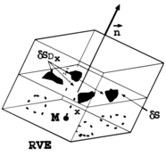
Figure 18. Definition of damage variable [61]

The damage value D(M, ${\textstyle \,{\overset {\rightarrow }{n}}}$, x) at point M in the direction ${\textstyle {\overset {\rightarrow }{n}}}$ and at abscissa x is defined as:

$D\left(M,{\overset {\rightarrow }{n}},x\right)={\frac {\delta {S}_{{D}_{x}}}{\delta S}}$

(18)

δS is the area of the intersection considered plan and the RVE, and ${\textstyle \delta {S}_{{D}_{x}}}$ is the effective area of intersections of all microcracks and microcavities in δS as illustrated in Figure 18. The anisotropic aspect of damage can be understood by assuming that the failure of the RVE depends on the direction on ${\textstyle {\overset {\rightarrow }{n}}}$. If microcracks and microcavities are uniformly distributed in the RVE, it's adequate to assume isotropic damage and damage variable D(M, ${\textstyle \,{\overset {\rightarrow }{n}}}$, x) doesn't depend on the direction, thus and scalar damage will control the deterioration.

To understand better the damage concept, let's consider the case of uniaxial tension force F with scalar damage variable. After reaching the maximum tensile strength and after occur of damage, the cross sectional area is reduced and becomes the effective cross sectional area S – SD. Where S is the original cross sectional area and SD is the total area of microcracks. The stress is no longer σ = F/ S but replaced by the effective stress σ₀ = F / (S − SD) = σ (1− D) ≥ σ. This concept can be extended to multiaxial stress state.

Physically, the degradation process of the virgin materials is due to the presence and growth of small fractures and micro voids. This growth process can be simulated within the context of the mechanics of continuous media, taking into consideration the theory of internal state variables, introducing an internal variable of damage represented by a scalar, vector or tensor. This internal variable of damage characterizes the level of damage in the material and transforms the stress real tensor into the so called "effective stress tensor" as follow:

${\boldsymbol {\sigma }}_{\mathit {\boldsymbol {0}}}={\boldsymbol {M}}^{-1}\,:{\boldsymbol {\sigma }}$

(19)

Mis a fourth-order tensor for anisotropic damage model. It's well approved that damage in concrete can be accepted to be isotropic. However, damage models using scalar damage variables are still preferred because of their simplicity in the formulation.

For isotropic damage mode, the material degradation is alike in all direction and the tensor M is reduced to M = (1-d) I, where I is an identity tensor. The equation (19) can be written for scalar-damage model:

${\boldsymbol {\sigma }}_{\mathit {\boldsymbol {0}}}={\frac {\boldsymbol {\sigma }}{\left(1-d\right)}}$

(20)

where d is an internal scalar variable range between 0 for no damage state and 1 for full distortion, σ₀ is effective stress tensor measured in the non-damaged space. The effective stress concept was formulated for the first time in connection with the equivalent deformation hypothesis by [62] as follow " The deformation associated to a damaged state subjected to a stress σ is equivalent to the deformation associated to the non-damage state subjected to an effective stress σ₀). A graphical representation of the effective and real space is illustrated in Figure 19.

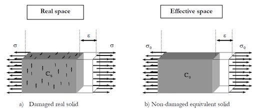
Figure 19. Graphic representation of the effective stress hypothesis presented by [57]

Continuum damage mechanics approach has been proved by many authors to be appropriate for constitutive models of concrete; different damage models have been proposed by researchers, among others [63], [64], [34], [65], [66], [67] [36].

Material deterioration in damage-based model is controlled by damage variable. The evolution law of damage, which plays a very important role in any damage-based model, is different for many continuum damage mechanics models. However, it is possible to group almost all existing approaches into three categories: one when the damage evolution law is imposed (e.g. [68,65,67]). Another approach is based on obtaining the damage evolution from a dissipation potential [69,61]. Third approach is based on using implicitly defined damage evolution law (e.g. [23,24,25], ).

2.3.3 Coupling between damage and plasticity

It is been widely accepted that coupling between damage and plasticity models is essential to capture the nonlinear behavior of concrete [26]. Coupled damage and plasticity models for concrete differ mainly in the coupling method and the damage evolution law.

In the implicit coupling, damage and plasticity are implicitly embedded in the yield and damage criteria [23,24,25], with the material strength being a decreasing function with respect to the damage variable. This implicit coupling characterizes the strength reduction due to the material deterioration and is equivalent to introducing effective instead of nominal stress into the yield function. Therefore, the concept of effective stress is still applicable in this case. This way of introducing coupling enables the constitutive modelling to use separate yield and failure criteria. The corresponding internal variables (damage variable and plastic strains for the coupled model) of the model do not explicitly depend on each other. Nevertheless, the parameter identification becomes more difficult as the model responses in this case are governed by all the internal variables used in the coupled model.

Other researchers describe coupling using a single function, in which only one loading function is specified and used to control the dissipation process. This function can be a damage loading function [68] or a yield function [22,61], the concept of effective stresses is applied by defining the yield function in the effective stresses space. In the first case with a damage loading function governing the dissipation process, an evolution law for the plastic strain is required [68]. For the use of a yield function, damage measure can be based on some criteria or by postulating damage variables law [22,61]. Figure 20 shows a representation of coupling between plasticity and damage [30].

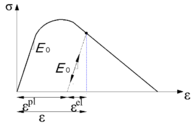
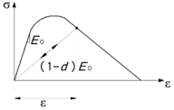
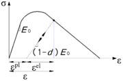
(a) Plasticity Model	(b) Damage Model	(c) Plastic Damage Model
Figure 20. Representation of coupling between damage and plasticity

In coupled models, plasticity for concrete can be described with isotropic hardening; however, damage in many cases is not isotropic but has preferential directions [70]. Some plastic isotropic damage models have been proposed, e.g. [21-23,25-29]; these models have shown good performance in capturing concrete behavior in tests on full-scale structures [70] [26]. Anisotropy can be added to the damage to capture the anisotropy feature of concrete both for compression and tension. Although anisotropic damage models are complex and coupling with plasticity in the application to practical engineering is not straightforward, researchers have investigated this issue and proposed plastic anisotropic damage models, among others [64,71-80].

Advantages and limitations of some coupled plastic damage models for concrete are presented briefly as follow:

Yazdani and Schreyer 1990 [81]: In this approach, the pressure-dependent damage surface is used as a failure surface, and enhanced with a Von Mises yield surface. In principal stress space, this yield surface covers the damage surface in the positive

hydrostatic axis, and lies almost entirely inside the damage surface in the opposite

direction Figure 21. Attention was also paid to the multi-axial behaviour of the

model, with the failure surface being calibrated to account for the strength enhancement and ductility under increasing lateral confinement Figure 21.

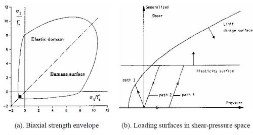
Figure 21. Coupled damage-plasticity model by Yazdani and Schreyer 1990 [81]

Compared to other coupled damage-plasticity models, this model is able to capture the irrecoverable strains using inelastic damage mechanism to account for the misfit of crack surfaces. Nevertheless, this capability is restricted to compressive mode of cracking only [81]. As a consequence, with a pure damage mechanism activated in tension, the model exhibits an inability to capture the observed permanent deformation in tensile loading.

Lee and Fenves 1998 [22]: This model has been developed for the numerical analysis of concrete dam, it was originally proposed for monotonic, cyclic and dynamic behavior by Lubliner et al.1989 [30]. In this model, a combined yield-failure surface is defined and evolves with damage variables, for which the evolution laws are postulated. The yield surface in two-dimensional principal stress space is shown in Figure 22.

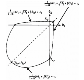
Figure 22. Yield surface in plane stress space Lee /Lubliner [22,30]

Yield criterion is based on a modified version of Drucker-Prager function. Stiffness deterioration is described by a scalar damage that is calculated as a function of the uniaxial damage variables in tension and compression. The opening/closing of microcracks also features in the model. This model has no damage loading function, and the evolution of the yield surface is governed by the damage variables.

Although the whole model is defined from several “pieces”, its thermodynamic

consistency can be readily ensured. However, the model showed very good performance in simulating concrete behavior under uniaxial and biaxial stress state, but is not recommend for high multiaxial stress state. This model is adopted in this research. The constitutive behavior, as well the implementation is presented in the next subsection.

Faria et al. 1998 [68]:

Similarly to the model of Lee and Fenves 1998 [22], this model possesses only one loading surface and was formulated on the basis of an effective stress tensor. However, in contrast with that by [22], a composite damage loading surface, instead of a yield surface, is used to govern the constitutive behavior of the model.

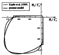
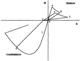
a) Initial 2D elastic domain	b) Uniaxial cyclic behavior
Figure 23. Coupled damage-plasticity model by Faria et al. 1998 [68]

The composite damage loading surface is formed by two separated damage surface, these function are used to define the strength envelope shown in Figure 23a. The evolution of damage variables in tension and compression are defined by law for each that contains three material parameters to be defined experimentally. This model showed good performance for biaxial and multiaxial loading, but fails to capture the permanent deformation in tension as shown in Figure 23b.

2.4 Concrete Plastic Damage Model

Since concrete behavior is brittle, but, under stress reversal, tensile cracks might close, then broken parts being reassembled. Therefore, concrete behavior can be better described with models that combine damage and plasticity. These models are particularly well suited for reproducing failure modes that are based on tensile cracking and compression crushing.

After the previous literature, in this work the coupled model of Lee and Fenves 1998 [22] is adopted. This model is described with a multiaxial model that considers parallel combination of scalar (isotropic) damaged elasticity and non-associated multi-hardening plasticity. This model is termed as “Concrete Plastic Damage Model” (CPDM) along this research. Was proposed for monotonic, cyclic and dynamic behavior by [30] and was further developed by [22]. This model shows good performance in primarily uniaxial and biaxial stress states, but should not be used in case of significant triaxial compressive stresses. Since the purpose of this research is to simulate the monotonic and cyclic behavior of RC structures where no serious triaxial compressive stresses are expected, hence, this model can be considered appropriate. The fundamental bases of this model are described in this subsection, necessary parameters to use the predefined model in the FEM software ABAQUS are also described. This subsection furnishes the base for the next subsection where a new methodology to define damage evolution is presented.

Going back to Figure 20, it displays uniaxial stress-strain plots typical of plasticity, damage and damage plasticity models; loading branches are represented with solid thick lines and unloading / reloading branches are plotted with dashed thin lines. E₀ is the initial (undamaged) elastic stiffness (deformation modulus), and ε^el and ε^pl are the elastic (recoverable) and plastic (irrecoverable) strain, respectively. Figure 20 shows that damage generates stiffness degradation [57] since the slope of unloading / reloading branch is (1  d) E₀ where d is a damage variable ranging between 0 (no damage) and 1 (destruction).

This models assumes that the main two failure mechanisms are tensile cracking and compressive crushing of the concrete material. The evolution of the yield (or failure) surface is controlled by two hardening variables, ${\textstyle {\epsilon }_{t}^{pl}}$ and ${\textstyle {\epsilon }_{c}^{pl}}$, linked to failure mechanisms under tension and compression loading, respectively. In Lee and Fenves 1998 [22] model, for uniaxial compression and tension, the stress-strain relation under uniaxial loading in displayed in Figure 20.c, can be written as:

${\sigma }_{c}\,=\left(1-{d}_{c}\right)\,{E}_{0\,}({\epsilon }_{c}-{\epsilon }_{c}^{pl})$

(21)

${\sigma }_{t}\,=\left(1-{d}_{t}\right)\,{E}_{0\,}({\epsilon }_{t}-{\epsilon }_{t}^{pl})$

(22)

where subindexes c and t refer to compression and tension, respectively.

For uniaxial cyclic loading-unloading conditions, Lee and Fenves 1998 [22] model assumes that the degradation in the elastic stiffness is given by

style="text-align: center;" $E=\left(1-d\right)\,{E}_{0}\,$

(23)

In equation (23), E is the reduced tangent stiffness and d is a scalar degradation variable, which is a function of stress state and of compression and tension damage variables (d_c and d_t, respectively):

$1-d=\left(1-{s}_{t}{d}_{c}\right)\,(1-{s}_{c}{d}_{t})\,$

(24)

In equation (24), s_c and s_t are dimensionless coefficients accounting for stress state and stiffness recovery effects, being given by

${s}_{c}=\,1-{h}_{c}\,(1-{r}^{\ast }\left({\sigma }_{11}\right))\,$	(25)
${s}_{t}=\,1-{h}_{t}\,{r}^{\ast }\left({\sigma }_{11}\right)\,$	(26)

In equations (25) and (26), ${\textstyle {\sigma }_{11}}$ is the first principal uniaxial stress (positive for tension), r* is a stress state parameter being ${\textstyle {r}^{\ast }\left({\sigma }_{11}\right)}$  = 1 for tension and ${\textstyle {r}^{\ast }\left({\sigma }_{11}\right)}$  = 0 for compression, and ${\textstyle {h}_{c}}$ and ${\textstyle {h}_{t}\,}$ are weighting factors ranging between 0 and 1. Factor ${\textstyle {h}_{c}}$ accounts for re-closing of cracks after tension-compression reversal; ${\textstyle {h}_{t}\,}$ represents recovery of crushed concrete after compression-tension reversal. If ℎ_c = 0.9 and ℎ_t = 0 for example; this means that 90% of the cracks close upon tension-compression reversal and the crushed concrete does not experience any recovery. Equations (25) and (26) show that ${\textstyle {s}_{c}}$ and ${\textstyle {s}_{t}}$ also range between 0 and 1.

For a better understanding of the effect of s_c and s_t coefficients, Figure 24 displays plots of uniaxial stress-strain loading-unloading behavior. The initial elastic branch with slope E₀ reaches the descending branch (Figure 27.b) at peak point 1, then cracking begins; later, unloading starts at point 2. At that point, there is no compression damage and d_c = 0, r* = 1, and s_c = 1; therefore, equation (24) shows that d = d_t. Consequently, the linear unloading branch has slope (1 d_t) E₀. In the way to stress reversing point 3, cracks begin closing. After point 3, r* = 0, s_c = 1 h_c, s_t = 1, d_c = 0, and equation (24) shows that d = (1 h_c) d_t. Therefore, the slope of the ongoing compression segment of the branch depends on parameter h_c; three options are plotted in Figure 24: (i) h_c = 0 (no crack is closed) with slope (1 d_t) E₀, (ii) h_c = 0.5 (half of the cracks are closed) with slope (1 0.5 d_t) E₀, (iii) h_c = 1 (all cracks are closed) with slope E₀. Noticeably, in the third option (h_c = 1), there is no compressive strength reduction. At point 4, an unloading branch arises; at that point, r* = 0, s_c = 1 h_c, s_t = 1, and equation (24) shows that 1 d = (1 d_c) [1 (1 h_c) d_t] = 1 d_c. Point 5 correspond again to stress reversal; after it, provided that h_t = 0, the slope of the ongoing branch is equal to (1 d_t) (1 d_c) E₀. Point 6 is the peak for the reduced tensile strength; after it, cracking reinitiates and a new descending branch is generated.

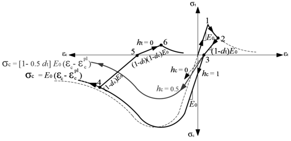
Figure 24. Uniaxial loading-unloading law

In this work and for cyclic loading simulation, ℎ_c = 0.9 is assumed in the main concrete bodies (90% of the stiffness in compression is recovered once cracks close), and lower values are taken in the zones where widely-opened cracks and bond-slip effects concentrate. ℎ_t = 0.0 is assumed for all the sections (referrer to subsection ‎6.1).

For multiaxial condition, the stress-strain relationship is given by:

${\boldsymbol {\sigma }}=\left(1-d\right)\,{\boldsymbol {D}}_{0}^{el}\,:({\boldsymbol {\epsilon }}-$${\boldsymbol {\epsilon }}^{pl})$

(27)

In equation (27), ${\textstyle {D}_{0}^{el}}$ is the elastic stiffness tensor, and ${\textstyle {\boldsymbol {\sigma }}}$ and ${\textstyle {\boldsymbol {\epsilon }}}$ are the stress and strain tensors, respectively. Scalar damage variable d keeps same meaning than for uniaxial condition, although replacing scalar factor ${\textstyle {r}^{\ast }}$ with a multiaxial one [22].

Regarding plasticity model, yield condition is based on the loading (yield) function F proposed in [30] with modifications suggested by [22] to account for different tension and compression strength evolution.

$F=\,{\frac {1}{1-\alpha }}\left(q-3\,\alpha \,p+\,\beta \,\left\langle {\sigma }_{max}\right\rangle -\right.$$\left.\gamma \,\left\langle -{\sigma }_{max}\right\rangle \right)-\,{\overline {{\sigma }_{c}}}=$$0$	(28)
$\alpha ={\frac {\left({f}_{b0}/{f}_{c0}\right)-1}{2\,\left({f}_{b0}/{f}_{c0}\right)-1}};\,\beta =$${\frac {\overline {{\sigma }_{c}}}{\overline {{\sigma }_{t}}}}\,\left(1-\alpha \right)-$$\left(1+\alpha \right);\,\gamma ={\frac {3\left(1-{K}_{c}\right)}{2\,{K}_{c}-1}}$	(29)

In equations (28) and (29), ${\textstyle \left\langle \cdot \right\rangle \,}$ is the Macaulay bracket, ${\textstyle p}$ is the hydrostatic pressure stress, ${\textstyle q}$ is the Von Mises-equivalent effective stress (effective stress accounts for stress divided by 1 d), and f_b0 and f_c0 are the biaxial and uniaxial compressive yield strengths, respectively; since f_b0 ≥ f_c0, α ranges between 0 (f_b0 = fc₀) and 0.5 (f_b0 ${\textstyle \gg }$ fc₀). ${\textstyle {\sigma }_{max}}$ is the maximum principal effective stress, and ${\textstyle {\overline {{\sigma }_{c}}}}$ and ${\textstyle {\overline {{\sigma }_{t}}}}$ are the effective compressive and tensile cohesion stress, respectively. ${\textstyle {\overline {{\sigma }_{c}}}}$ and ${\textstyle {\overline {{\sigma }_{t}}}}$ are defined as ${\textstyle {{\overline {{\sigma }_{c}}}=\sigma }_{c}\,/\left(1-\right.}$$\left.{d}_{c}\right)$ and ${\textstyle {{\overline {{\sigma }_{t}}}=\sigma }_{t}\,/\left(1-\right.}$$\left.{d}_{t}\right)$ . K_c is the ratio of second stress invariants on tensile and compressive meridians.

The plasticity model assumes non-associated potential plastic flow. The flow potential G is the Drucker-Prager hyperbolic function given by:

$G={\sqrt {{\left(\epsilon \,{\sigma }_{t0}\mathrm {tan} \,\psi \,\right)}^{2}+{q}^{2}}}\,-$$\,p\mathrm {tan} \,\psi$

(30)

In equation (30), σ_t0 is the uniaxial tensile stress at failure, ϵ is the eccentricity of plastic potential surface, and ѱ is the dilatancy angle measured in ${\textstyle p}$- ${\textstyle q}$ (deviatory) plan at high confining pressure.

As discussed previously, K_c is the ratio between the magnitudes of deviatoric stress in uniaxial tension and compression; K_c ranges between 0.5 (Rankine yield surface) and 1 (Von Mises). In this study, K_c is obtained from the Mohr-Coulomb yield surface function in cylindrical coordinates [57]:

$H\left(\rho ,\,x,\theta ,\phi ,c\right)=\,{\sqrt {2}}\,x\,sin\,\phi +{\sqrt {3}}\,\rho \,cos\,\theta -$$\rho \mathrm {sin} \,\theta \,sin\phi -{\sqrt {6}}\,c\,cos\phi =0$

(31)

In equation (31), ρ is the octahedral radius, ξ is the distance from the origin of stress space to the stress plan, θ is the Lode similarity angle, ϕ is the friction angle, and c is the cohesion. In equation (31), ${\textstyle r=}$${\sqrt {2\,{J}_{2}}}$, ξ = I₁ / ${\textstyle {\sqrt {3}}}$, and ${\textstyle \mathrm {sin} \,q=}$${\frac {3{\sqrt {3}}{J}_{3}}{2{J}_{2}^{3/2}}}$; I₁ is the first invariant of stress tensor and J₂ and J₃ are the second and third invariants of deviatoric stress tensor, respectively.

For ${\textstyle x}$ = 0 and θ = ± π / 6 (negative/positive for tension/compression meridian plans), the magnitudes of deviatory stress in uniaxial compression and tension at yield (ρ_c0 and ρ_t0) and K_c are

$\,{\rho }_{c0}=\,{\frac {2\,c\,{\sqrt {6}}\,cos\phi \,}{3-sin\phi \,}}$ ${\rho }_{t0}=\,{\frac {2\,c\,{\sqrt {6}}\,cos\phi }{3+sin\phi }}$ ${K}_{c}\,={\frac {{\rho }_{t0}}{{\rho }_{c0}}}={\frac {3-sin\phi }{3+sin\phi }}$

(32)

By assuming that ϕ = 32° [57], last equation in (32) shows that K_c = 0.7. Figure 25 represents the yield surface in deviatory plan for several values of K_c ranging from 0.5 to 1. CM and TM account for compression/tension meridian plans, respectively.

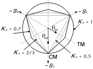
Figure 25. Yield surface in the deviatory plan for several values of Kc

Equations (30), (28) and (29) show that the concrete behavior depends on four constitutive parameters K_c, ѱ, f_b0 / f_c0, ϵ; it can be assumed that ѱ =13° [82]. Table 3 describes the values used in this study.

Table 3. Parameters of CPDM

Kc	Ѱ (º)	fb0 / fc0	ϵ
0.7	13	1.16	0.1

Since this model uses the concept of effective stresses as it’s indicated in equations (27), (28) and (29), as well, the cyclic uniaxial and multiaxial behavior is dominated by the same variables. All these direct influences of damage variables make the approach to calculate them an essential issue. Defining these variables is a hard task, as no clear guide is available to calculate and implement such variables in the CPDM of Abaqus software. Next section presents a new approach for calculating and implementing these variables in CPDM, the proposed approach can be uses for the model already implemented in Abaqus, as well as any model requires the damage evolution to be defined.

3. Proposed methodology for calculating damage variables of CPDM

3.1 Introduction

As described before, damage evolution law plays a significant role in any damage model, particularly when this law is imposed. An important number of researchers have proposed different damage evolutions laws. Most of them are based on splitting damage into compressive and tensile parts and each one is determined separately by its evolution law; total damage is calculated with some combination rules e.g. [68], [83], [80], [84]. Few evolution laws are based on general formulae for calculating damage in compression and tension [85]. In most of the available damage evaluating formulae the parameters need to be calibrated experimentally. Following some approaches that can be used to calculate the damage evolution for CPDM:

• Mazars, Pijaudier-Cabot 1989 [34]. Defined a formula to calculate the total scalar damage as the sum of the uniaxial compressive and tensile damage evolution. The model is originally developed by Mazars 1984-1986 ( [33] [86]), and formulated in the next formula

${\textstyle d={\alpha }_{t}{d}_{t}+\,{\alpha }_{c}{d}_{c}}$

(33)

d_t and d_c are the damage evolution for uniaxial tension and compression respectively, α_t and α_c are weight factor and can be calculated according to [33]. Uniaxial damage evolution is presented in the following formulation, "i" takes the same meaning for "c" compression and "t" tension.

${d}_{i}=\,1-\,{\frac {\left({1-A}_{i}\right){K}_{0}}{\overline {\epsilon }}}-{\frac {{A}_{i}}{exp\left[{B}_{i}\left({\overline {\epsilon }}-{K}_{0}\right)\right]\,}}\,$

(34)

${\textstyle {\overline {\epsilon }}}$ is the equivalent strain, and the parameters A_c, A_t, B_c, B_t and K₀ are derived from compression test on cylinders and bending test on beams.

• Birtel, Mark 2006 [83]. Tension and compression damage variables "damage evolution" are calculated by assuming constant ratios between compressive plastic and crushing strains, and between tensile plastic and cracking strains, respectively. The uniaxial damage evolution is presented in the next formulation, "i" takes the same meaning for "c" compression and "t" tension.

${d}_{i}=\,1-\,{\frac {{\sigma }_{i}{E}_{0}^{-1}}{{\epsilon }_{i}^{pl}\left({\frac {1}{{b}_{i}}}-1\right)+{\sigma }_{i}{E}_{0}^{-1}}}\,$

(35)

E₀ is the original concrete stiffness modulus, ε^pl is the uniaxial plastic strain, b_i is a parameter that needs to be calibrated from cyclic uniaxial tension and compression tests.

• Häussler-Combe, Hartig 2008 [85]. Defined a scalar damage evolution function with three material parameters. Damage function is given in the next formulation:

$D=\,1-{e}^{-{\left[{\frac {\left({k}_{d}-{e}_{d0}\right)}{{e}_{d}}}\right]}^{{g}_{d}}}\,\,$

(36)

k_d is the equivalent damage strain variable defined in [85], e_d0, e_d and g_d are material parameters to be calibrated with experimental results.

• Yu et al. 2010 [87]. This work focuses on confined concrete. A linear expression of damage variable vs. stress is proposed for the compressive descending branch (compressive damage) as follow:

$d=\,1-\,{\frac {{\sigma }_{c}}{{f}_{c0}^{'}}}\,$

(37)

Where ${\textstyle {f}_{c0}^{'}}$ is the maximum strength of concrete. For constant confinement pressure, the damage function becomes:

$d=\,1-\,{\frac {{\sigma }_{c}-\,{\frac {1+C+2A}{1-A}}{\sigma }_{1}}{{f'}_{cc}^{\ast }-{\frac {1+C+2A}{1-A}}{\sigma }_{1}}}$

(38)

${\textstyle {f'}_{cc}^{\ast }}$ the maximum concrete strength under constant confining pressure, σ₁ is the confining pressure, C and A are material parameters need to be calibrated from experiments.

• Zheng et al. 2012 [88]. Modified the function developed by Mazars, Pijaudier-Cabot 1989 [34], uniaxial damage evolution function is presented as follow:

${d}_{i}=\,1-\,{\frac {{1-A}_{i}}{1+{\frac {{k}_{i}^{d}}{{\epsilon }_{i}^{f}}}}}-{\frac {{A}_{i}}{exp\left[{B}_{i}{\frac {{k}_{i}^{d}}{{\epsilon }_{i}^{f}}}\right]\,}}\,$

(39)

${\textstyle {\epsilon }_{i}^{f}}$ is defined as the pick value of strain when damage occurs, ${\textstyle {k}_{c}^{d}}$ and ${\textstyle {k}_{t}^{d}}$ are calculated according to [Zheng et al. 2012], A_c, A_t, B_c, B_t shall be calibrated form experiments.

• López-Almansa et al. 2014 [84]. Damage variables are determined by an iterative empirical procedure aiming to fit experimental results. The damage evolution function for compression and tension is presented as follow:

${d}_{i}=\,1-\,{e}^{\left(-{a}_{i}{\epsilon }_{i}^{pl}\right)}\,$

(40)

Parameters a_c, a_t needs to be calibrated from the uniaxial tension and compression stress-strain behavior.

After these investigations, this section proposes a new approach for obtaining damage variables. The need of proposing a new methodology arises from their advantages:

• Is based on the formulation by Lubliner and Lee/Fenves, which is the base for the ABAQUS plastic damage model for concrete. The proposed approach modifies this formulation and obtains closed-form expressions of the damage variables in terms of the corresponding strains; these expressions are derived after integration of concrete fracture and crushing energy.

• No calibration with experimental results is required.

• Implementation is particularly easy.

• Results are insensitive of mesh size, since a strategy aiming to avoid mesh-dependency is incorporated.

All these advantages make this methodology well suited for practical applications. Noticeably, the default ABAQUS model based on the Lubliner/Lee/Fenves approach requires that the uniaxial damage variables (i.e. the damage evolution) are provided by the user, and no guidelines are provided. Therefore, defining the damage evolution is a big concern for any user of the Concrete Damage Plastic Model. In the proposed model, constant mesh size is required in the elements corresponding to the same material. If elements with different size are employed for a single material, their parameters should be defined individually for each size following the proposed methodology.

This approach can consider any concrete constitutive law, either empirical (e.g. like formulations commonly recommended by design codes) or directly based on particular experiments; noticeably, any such constitutive law should account for mesh-sensitivity. In this paper, a particular algorithm that uses laws based on European recommendations is derived; in this case, the only input parameters are concrete compressive strength and mesh size. This algorithm is implemented in the software package ABAQUS [89]; could be also implemented in other computer codes that contain Plastic Damage Model and that require values of damage variables.

Next subsections describe the bases of the proposed approach as well as its implementation for CPDM. Mesh-insensitivity is validated in a simple tension example, accuracy and reliability are also verified by simulating a cyclic experiment on plain concrete specimens. Furthermore, three laboratory experiments are described with the proposed approach to investigate its capability to reproduce the behavior of reinforced concrete (RC) framed structures under monotonic and cyclic loading.

3.2 General description

The proposed approach for calculating the damage variables starts from definition of compressive and tensile variables as the portion of normalized energy dissipated by damage:

${\,d}_{c}\,={\frac {1}{{\,g}_{c}}}\int _{0}^{{\epsilon }_{c}^{ch}}{\sigma }_{c}\,d{\epsilon }_{c}^{ch}$ ${\,d}_{t}\,={\frac {1}{{\,g}_{t}}}\int _{0}^{{\epsilon }_{t}^{ck}}{\sigma }_{t}\,d{\epsilon }_{t}^{ck}$

(41)

In equation (41), ${\textstyle {\epsilon }_{c}^{ch}}$ and ${\textstyle {\epsilon }_{t}^{ck}}$ are the crushing and cracking strains respectively, see Figure 27. Normalization coefficients g_c and g_t represent the energies per unit volume dissipated by damage along the entire deterioration process:

${\,g}_{c}\,=\int _{0}^{\infty }{\sigma }_{c}\,d{\epsilon }_{c}^{ch}$ ${\,g}_{t}\,=\int _{0}^{\infty }{\sigma }_{t}\,d{\epsilon }_{t}^{ck}$

(42)

Equations (41) and (42) show that d_c and d_t range between 0 (no damage) and 1 (destruction). Figure 26 describes the meaning of g_c and g_t.

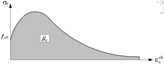
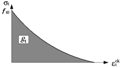
a) Compression (gc)	b) Tension (gt)
Figure 26. Parts of energy dissipated by damage

Noticeably, the energies per unit area and per unit volume are related by ${\textstyle {\,g}_{c}\,=}$${\,G}_{ch\,}/\,{l}_{eq}$ and ${\textstyle {\,g}_{t}\,={\,G}_{F}\,/{\,l}_{eq}}$; ${\textstyle {\,G}_{ch}}$ and ${\textstyle {\,G}_{F}}$ are material parameters defined as crushing and fracture energies and ${\textstyle {\,l}_{eq}}$ is the characteristic length of the element (subsection ‎3.3).

Relation between compressive and tensile stress and, respectively, crushing and cracking strain, is established, according to [30], as:

${\sigma }_{c}={f}_{c0}\left[\left(1+{a}_{c}\right)exp\left(-{b}_{c\,}{\epsilon }_{c}^{ch}\right)-\right.$$\left.{a}_{c}exp\left(-{2b}_{c\,}{\epsilon }_{c}^{ch}\right)\right]$	(43)
${\sigma }_{t}={f}_{t0}\left[\left(1+{a}_{t}\right)exp\left(-{b}_{t\,}{\epsilon }_{t}^{ck}\right)-\right.$$\left.{a}_{t}exp\left(-{2b}_{t\,}{\epsilon }_{t}^{ck}\right)\right]$	(44)

In equations (43) and (44), f_c0 and f_t0 and are the compressive and tensile stresses that correspond to zero crushing ( ${\textstyle {\epsilon }_{c}^{ch}=}$$0$) and to onset of cracking ( ${\textstyle {\epsilon }_{t}^{ck}=}$$0$), respectively; see Figure 26. As well, a_c, a_t, b_c and b_t are dimensionless coefficients to be determined. Replacing equations (43) and (44) in equation (42), provides the following relations among g_c and g_t and such coefficients:

${g}_{c}={\frac {{f}_{c0}}{{b}_{c\,}}}\left(1+{\frac {{a}_{c\,}}{2}}\right)$ ${g}_{t}={\frac {{f}_{t0}}{{b}_{t\,}}}\left(1+{\frac {{a}_{t\,}}{2}}\right)$

(45)

Coefficients b_c and b_t can be obtained by replacing ${\textstyle {g}_{c}\,=}$${\,G}_{ch}\,/\,{l}_{eq}$ and ${\textstyle {\,g}_{t}\,={\,G}_{F}\,/\,{l}_{eq}\,}$ in equation (45):

${b}_{c}={\frac {{f}_{c0\,}{l}_{eq}}{{G}_{ch\,}}}\,\left(1+{\frac {{a}_{c\,}}{2}}\right)$ ${b}_{t}={\frac {{f}_{t0\,}{l}_{eq}}{{G}_{F\,}}}\,\left(1+{\frac {{a}_{t\,}}{2}}\right)$

(46)

By substituting results (43) through (45) in equation (41), the proposed tensile and compressive damage functions are derived:

${\,d}_{c}\,=1-{\frac {1}{2+{a}_{c}}}\left[2\,\left(1+{a}_{c}\right)\,exp\left(-\right.\right.$$\left.\left.{b}_{c\,}{\epsilon }_{c}^{ch}\right)-{a}_{c}\,exp\left(-{2\,b}_{c\,}{\epsilon }_{c}^{ch}\right)\right]$	(47)
${\,d}_{t}\,=1-{\frac {1}{2+{a}_{t}}}\left[2\,\left(1+{a}_{t}\right)\,exp\left(-\right.\right.$$\left.\left.{b}_{t\,}{\epsilon }_{t}^{ck}\right)-{a}_{t}\,exp\left(-{2\,b}_{t\,}{\epsilon }_{t}^{ck}\right)\right]$	(48)

Therefore, provided that coefficients a_c and a_t are not zero:

$exp\left(-{b}_{c\,}{\epsilon }_{c}^{ch}\right)={\frac {1}{{a}_{c}}}\left[1+{a}_{c}-\right.$$\left.{\sqrt {1+{a}_{c}\,\left(2+{a}_{c}\right)\,{d}_{c}}}\right]$	(49)
$exp\left(-{b}_{t\,}{\epsilon }_{t}^{ck}\right)={\frac {1}{{a}_{t}}}\left[1+{a}_{t}-\right.$$\left.{\sqrt {1+{a}_{t}\,\left(2+{a}_{t}\right)\,{d}_{t}}}\right]$	(50)

By zeroing derivatives of σ_c and σ_t (equations (43) and (44), respectively) with respect to, respectively, crushing and cracking strain, maximum values f_cm and f_tm (Figure 27) are obtained:

${f}_{cm}={\frac {{f}_{c0}{\left(1+{a}_{c}\right)}^{2}}{4{\,a}_{c}}}$ ${f}_{tm}={\frac {{f}_{t0}{\left(1+{a}_{t}\right)}^{2}}{4{\,a}_{t}}}$

(51)

Equations (51) provide:

${a}_{c}=2\,\left({\frac {{f}_{cm}}{\,{f}_{c0}}}\right)-1+2\,{\sqrt {{\left({\frac {{f}_{cm}}{{\,f}_{c0}}}\right)}^{2}-\left({\frac {{f}_{cm}}{\,{f}_{c0}}}\right)}}$	(52)
${a}_{t}=2\,\left({\frac {{f}_{tm}}{{\,f}_{t0}}}\right)-1+2\,{\sqrt {{\left({\frac {{f}_{tm}}{\,{f}_{t0}}}\right)}^{2}-\left({\frac {{f}_{tm}}{\,{f}_{t0}}}\right)}}$	(53)

These developments complete the description of the proposed methodology. Parameters a_c, a_t, b_c and b_t can be determined from equations (52), (53) and (46) in terms of f_cm, f_c0, f_tm, f_t0, l_eq, G_ch and G_F. Then, the damage functions can be calculated according equations (47) and (48). An implementation of the proposed approach using the concrete behavior described in next subsection is presented in subsection ‎3.4.

3.3 Uniaxial concrete behavior

This subsection describes the concrete uniaxial stress-strain law that is selected for implementation. Figure 27.a and Figure 27.b explain the compressive and tensile models, respectively; noticeably, tensile model is smeared, i.e. strain includes both crack opening and actual tensile strain between cracks. Figure 27 displays the constitutive laws (thick solid lines) and the unloading / reloading branches (thin dashed lines). Figure 27 corresponds to the damage-plasticity behavior depicted in Figure 20.c. The ascending compressive segments in Figure 27.a follow the Model Code recommendations [90] and the descending segment is engendered as [28]. Tensile stress-strain relation consists of an initial linear segment and a nonlinear descending branch [91] [92], as shown in Figure 27.b. Both compressive and tensile descending branches are generated to ensure nearly mesh-independency; the regularization approach is based on selecting the softening branches of concrete constitutive laws depending on mesh size. In Figure 27, f_cm and f_tm represent compressive and tensile stress strength, respectively; corresponding strains are ε_cm and ε_tm, respectively. According to [90], it is assumed that ε_cm = 0.0022, f_cm = f_ck + 8 (f_ck is the characteristic value of concrete compressive strength), and ${\textstyle \,{f}_{tm}\,=}$$0.3016\,{f}_{ck}^{2/3}$; these stresses and the deformation modulus are expressed in MPa. In Figure 27.a, ${\textstyle {\epsilon }_{c}^{ch}}$ and ${\textstyle {\epsilon }_{0c}^{el}}$ are the crushing and elastic undamaged components of strain; ${\textstyle {\epsilon }_{c}^{pl}}$ and ${\textstyle {\epsilon }_{c}^{el}}$ are the plastic and elastic damaged components. In Figure 27.b, ${\textstyle {\epsilon }_{c}^{ck}}$ and ${\textstyle {\epsilon }_{0t}^{el}}$ are the cracking and elastic undamaged strain components; ${\textstyle {\epsilon }_{t}^{pl}}$ and ${\textstyle {\epsilon }_{t}^{el}}$ are the plastic and elastic damaged components.

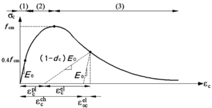
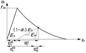
a) Compression	b) Tension
Figure 27. Assumed uniaxial model of concrete behavior

First segment in Figure 27.a is linear, ${\textstyle {\,\sigma }_{c(1)}=}$${E}_{0}\,{\epsilon }_{c}$, reaching 0.4 f_cm; second (ascending) segment (in between 0.4 f_cm and f_cm) is quadratic [90]:

${\sigma }_{c(2)}=\,{\frac {{E}_{ci\,}\,{\frac {{\epsilon }_{c}}{{f}_{cm}}}-\,{\left({\frac {{\epsilon }_{c}}{{\epsilon }_{cm}}}\right)}^{2}}{1+\left({E}_{ci\,}{\frac {{\epsilon }_{cm}}{{f}_{cm}}}-2\right)\,{\frac {{\epsilon }_{c}}{{\epsilon }_{cm}}}}}{f}_{cm}$

(54)

In equation (54), E_ci is the modulus of deformation of concrete for zero stress, given by ${\textstyle {\,E}_{ci}=}$$10000\,{{f}_{cm}}^{1/3}$ and E₀ = (0.8 + 0.2 f_cm / 88) E_ci (in MPa) [90]. In the initial linear branch, E₀ is the secant modulus that corresponds to 0.4 f_cm stress.

Third (descending) segment is given by:

${\sigma }_{c(3)}=\,{\left({\frac {2+\,{\gamma }_{c}\,{f}_{cm}{\,\epsilon }_{cm}}{2\,{f}_{cm}}}-{\gamma }_{c}{\,\epsilon }_{c}+{\frac {{\,{\epsilon }_{c}^{2}\,\gamma }_{c\,}}{2\,{\epsilon }_{cm}}}\right)}^{-1}$	(55)
${\gamma }_{c}=\,{\frac {{\pi }^{2}{\,f}_{cm\,}{\epsilon }_{cm\,}\,}{2{\left[{\frac {{G}_{ch}}{{l}_{eq}}}-0.5\,{f}_{cm\,}\left({\epsilon }_{cm\,}\left(1-b\right)+b\,{\frac {{f}_{cm\,}}{{E}_{0\,}}}\right)\right]}^{2}}}$ $\qquad b={\frac {{\epsilon }_{c}^{pl}\,}{{\epsilon }_{c}^{ch}}}$	(56)

In equations (55) and (56), G_ch is the crushing energy per unit area [28], and l_eq is the characteristic length, which depends on the mesh size, the type of finite element and the crack direction [93] [28] [94]. Assuming idealized behavior of single band of cracks, the characteristic length can be determined after the mesh size; [95] relate the crack width with the square root of the finite element area for 2D elements. In this work, brick solid elements are utilized; the characteristic length is taken as average length of the brick element.

Based on experimental observations, b = 0.9 (equation (56)) can be initially assumed. After calculating the damage variables, the average value of b along the relevant strain range is obtained; iterative calculations are performed until reaching convergence. The final value of b affects the softening branch of the compressive stress-strain relation (equations (55) and (56)); therefore, the dissipated crushing energy will be changed. Anyway, this effect is not very intense.

Equation (55) shows that the descending branch approaches asymptotically zero; therefore, a fictitious maximum strain shall be selected for calculation purposes. The maximum strain value shall fulfill that the crushing energy in equation (60) is equal to the area under the corresponding compressive stress-strain law multiplied by the characteristic length.

Regarding tensile behavior, the ratio between tensile stress σ_t(w) (for crack width w) and maximum tensile strength f_tm, is given by [96]:

$\,{\frac {{s}_{t}(w)}{{f}_{tm}}}=\,\left[1+\,{\left({c}_{1}{\frac {w}{{w}_{c}}}\right)}^{3}\right]{e}^{-{c}_{2}\,{\frac {w}{{w}_{c}}}}\,-$${\frac {w}{{w}_{c}}}\left(1+{c}_{1}^{3}\right)\,{e}^{-{c}_{2}}$

(57)

In equation (57), c₁= 3, c₂= 6.93 [96], and w_c is the critical crack opening. Equation (57) shows that σ_t(0) = f_tm and σ_t(w_c) = 0. Therefore, w_c can be considered as the fracture crack opening. Equation (58) [96] relates w_c with the tensile strength and fracture energy G_F per unit area:

${\,w}_{c}=5.14\,{G}_{F}\,/{f}_{tm}\,$

(58)

According to [90], G_F (N/mm) can be calculated as

${G}_{F}=0.073\,{f}_{cm}^{0.18}$

(59)

In equation (59), f_cm is expressed in MPa. The ratio between crushing and fracture energies can be assumed proportional to square of the ratio between compressive and tensile strengths [94]:

${G}_{ch}={\left({\frac {{f}_{cm}}{{f}_{tm}}}\right)}^{2}{G}_{F}$

(60)

In this work, the actual crack spacing is not studied, it has been assumed that there is a single crack per element. This supposition is suitable for global-purpose simulation. After this assumption, in the descending segment of the tensile stress-strain curve (Figure 27.b), the strain can be obtained in terms of the crack opening from the following kinematic relation:

${\,\epsilon }_{t}\,={\epsilon }_{tm}+w\,/\,{l}_{eq}$

(61)

This subsection describes the concrete uniaxial concrete behavior; next subsection describes their implementation in the proposed approach.

3.4 Implementation

Following the formulation described in the previous subsection, coefficients a_c, a_t, b_c and b_t (subsection ‎3.2) can be determined. Coefficient a_c is obtained by replacing f_c0 = 0.4 f_cm (Figure 27.a) in equation (52). Figure 27.b shows that f_tm = f_t0, then equation (53) shows that a_t = 1. Coefficient b_c can be determined from equation (46) by replacing f_c0 = 0.4 f_cm = 0.4 (f_ck + 8) MPa. Coefficient b_t is determined by replacing a_t = 1 and ${\textstyle {f}_{t0}\,=}$${f}_{tm}\,=0.3016\,{f}_{ck}^{2/3}$ [90] in equation (46). Therefore:

${a}_{c}=7.873$ ${a}_{t}=1$ ${b}_{c}={\frac {1.97({f}_{ck}\,+\,8)}{{G}_{ch}}}{l}_{eq}$ ${b}_{t}={\frac {0.453{f}_{ck}^{2/3}}{{\boldsymbol {\,}}{\,G}_{F}}}{l}_{eq}$

(62)

In the last two expressions in equation (62), f_ck is expressed in MPa. After parameters a_c, a_t, b_c and b_t, damage variables d_c and d_t are determined by equations (47) and (48) in terms of crushing and cracking strain, respectively.

A particular implementation of the proposed methodology by using the previously described concrete constitutive law is described next. All stress values are in MPa.

1. The input data are the concrete compressive strength f_ck, the parameters in Table 3, the mesh size ${\textstyle {l}_{eq}}$, and the ratio b (eqn. (56)). Initial assumption is b = 0.9

2. Calculate the compressive / tensile stress strength f_cm = f_ck + 8 / ${\textstyle {f}_{tm}\,=}$$0.3016\,{f}_{ck}^{2/3}$

3. State the strain at compressive stress strength as ε_cm = 0.0022

4. Calculate the initial tangent modulus of deformation of concrete ${\textstyle {\,E}_{ci}=}$$10000\,{{f}_{cm}}^{\frac {1}{3}}$ and the undamaged modulus of deformation ${\textstyle {\,E}_{0}=}$${\,E}_{ci}(0.8+0.2{\frac {{f}_{cm}}{88}})$

5. Calculate the fracture / crushing energy (N/mm) ${\textstyle {G}_{F}=}$$0.073\,{f}_{cm}^{0.18}$ / ${\textstyle {G}_{ch}={\left({\frac {{f}_{cm}}{{f}_{tm}}}\right)}^{2}{G}_{F}}$

6. Calculate the critical crack opening ${\textstyle {\,w}_{c}=}$$5.14\,{G}_{F}\,/\,{f}_{tm}$

7. Build the first / second / third segments of the concrete uniaxial compressive law: ${\textstyle {\sigma }_{c(1)}=}$${E}_{0}\,{\epsilon }_{c}$ / eqn. (54) / eqn. (55). In eqn. (55), strain is bounded; the selected upper bound should fulfill the condition that the crushing energy G_ch (equation (60)) is reached

8. Build the first / second segment of the concrete uniaxial tensile law: ${\textstyle {\sigma }_{t(1)}=}$${E}_{0}\,{\epsilon }_{t}$ / eqns. (57) and (61)

9. Calculate the damage parameters according equation (62): ${\textstyle {a}_{c}=}$$7.873$; ${\textstyle {a}_{t}=1}$; ${\textstyle {b}_{c}=}$${\frac {1.97({f}_{ck}\,+\,8)}{{G}_{ch}}}{l}_{eq}$; ${\textstyle {b}_{t}=}$${\frac {0.453{f}_{ck}^{2/3}}{{\boldsymbol {\,}}{\,G}_{F}}}{l}_{eq}$

10. Calculate the compressive / tensile damage variables (damage evolution) according to eqns. (47) / (48)

11. Calculate the compressive and tensile plastic strains as indicated in Figure 27: ${\textstyle {\epsilon }_{c}^{pl}\,=}$${\epsilon }_{c}^{ch}-{\sigma }_{c}{d}_{c}/\left(1-{d}_{c}\right)\,{E}_{0\,}$ , ${\textstyle {\epsilon }_{t}^{pl}\,=}$${\epsilon }_{t}^{ck}-{\sigma }_{t}{d}_{t}/\left(1-{d}_{t}\right)\,{E}_{0\,}$

12. Calculate the average value of ratio ${\textstyle b={\frac {{\epsilon }_{c}^{pl}\,}{{\epsilon }_{c}^{ch}}}}$ and compare with the assumption in step ‎1. Repeat until reaching convergence.

Once convergence is reached, the major output are curves of compressive / tensile stress and damage variables vs. crushing / cracking strain, respectively. These plots constitute the input of the implementation in any model describing the global structural behavior. This algorithm is suited for software package ABAQUS [89] [97] [98]. Noticeably, the proposed approach can be also fitted for other computer codes and for other concrete formulations, either empirical (code-type) or directly based on experiments. A flow chart of the methodology implementation is displayed in Figure 28.

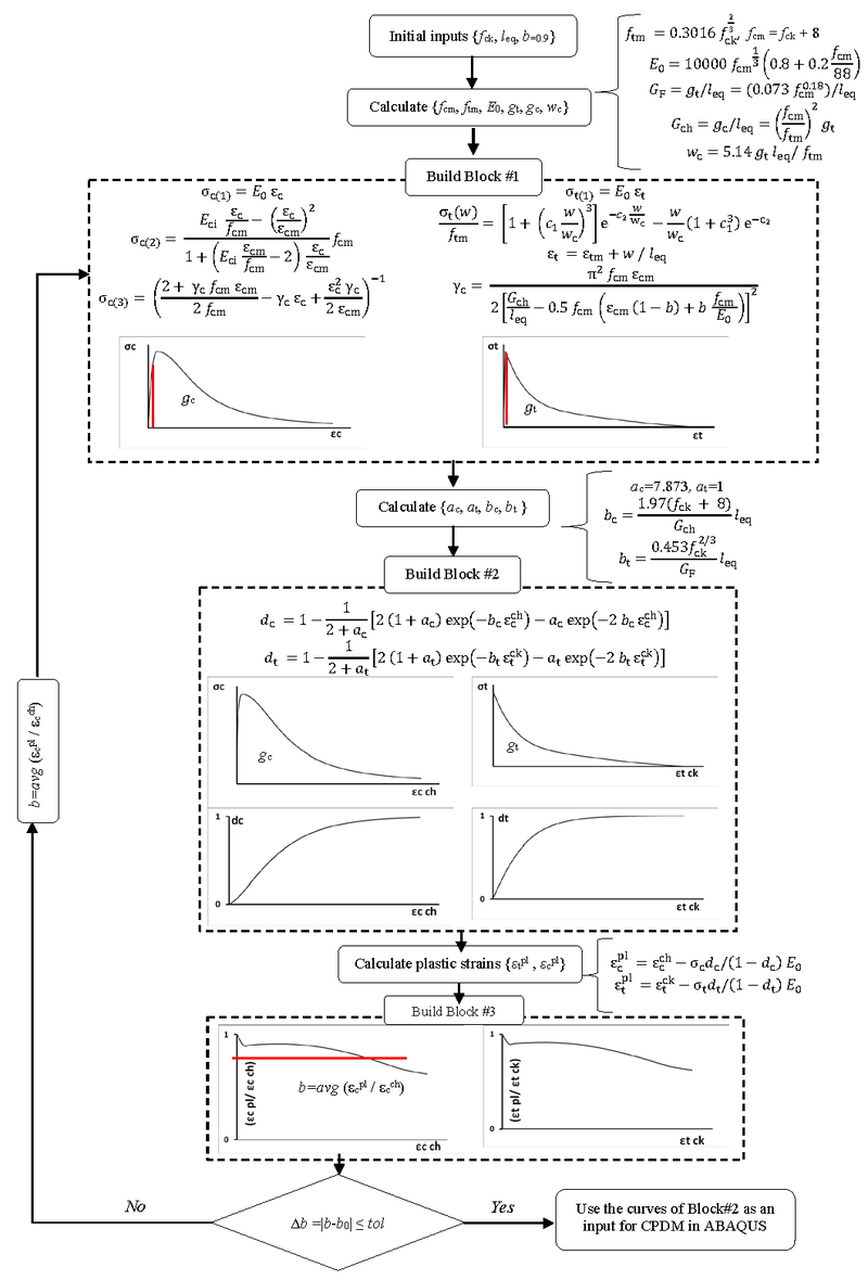
Figure 28. Flow chart of the proposed methodology implementation

3.5 Mesh insensitivity verification

When the material exhibits softening, finite element size influences significantly the entire model behavior due to localization since the dissipated energy decreases upon mesh refinement. This can be solved by the so-called mesh regularization techniques. One of the simplest remedy is the Crack Band Method; it uses energy-based scaling of the softening part of the stress-strain relation [99]. This technique can be considered as a simple and effective method for practical engineering analysis and has been implemented in many concrete plastic damage models, among others [21] [78]. More advanced techniques are the so-called Non-Local approaches; they are based on introducing non-locality in the constitutive model. This non-locality can be incorporated into an integral format [100] [100]; this approach has been implemented in different plastic damage models [101] [26]. Another strategy for incorporating non-locality is including higher-order deformation gradients in the model [102]. This has been implemented in several plastic damage models [103] [104].

As the model of [30] is the base of this work and this model uses the fracture energy-based regularization to describe the softening in tension and compression, the crack band technique is considered. Then both fracture and crushing energies are scaled in relation to the finite element size. The main assumption in this technique is that damage is localized in a single raw of elements; this is true for the physical failure mechanism of concrete in tension but is not exactly right for compression. Uniaxial compression tests show a great relation between boundary conditions, concrete strength, size, and failure mechanism [105] [106]. It varies between cone failure and vertical splitting modes. Cone failure occurs when friction at top and bottom sections restraints lateral expansion; this mode is characterized by inclined slip bands at each corner and crushing in the middle zone for very stocky specimens. Vertical splitting mode can happen for highly slender specimens when the effect of friction is neglectable. Intermediate scenarios can occur for different degrees of friction and slenderness; they are characterized mainly by inclined shear band zone. Regarding damage localization under compression, experimental observation by [105] [92] [107] showed strain localization; analytical investigation by [108] showed that the concept of fracture energy in tension holds true for compression. This gives the evidence to use the fracture energy-based regularization in describing the softening of concrete under compression [109].

In this subsection the capacity of proposed methodology to overcome mesh insensitivity is verified for a uniaxial tension problem. Given the above considerations, it is apparent that the uniaxial compression case cannot be verified in the same way. For practical engineering applications, behavior is mainly controlled by bending and there will be mixed stresses states with high stress gradients; therefore, the possible inaccuracies will have little effect on overall results.

This subsection describes the application of the proposed methodology to the problem of uniaxial tension of a 200 mm × 200 mm × 200 mm cube, as described in Figure 29. The cube is discretized with a uniform mesh of 3D 8-node hexahedron solid finite elements (C3D8R). Figure 29 displays three sketches of the cube discretized with a coarse mesh (l_eq = 200 mm, one element), a medium mesh (l_eq = 50 mm, 64 elements) and a fine mesh (l_eq = 25 mm, 512 elements), respectively. The objective of this analysis is to verify the allegedly low sensitivity to mesh size.

This problem is analyzed with the algorithm described in subsection ‎3.4. Table 4 displays the values of the parameters for each mesh size. Any of the values of parameter b in Table 4 is the result of an independent iterative process starting from 0.9. For consistency, the final value is independent on this initial assumption.

The algorithm is implemented in ABAQUS code [89]. The displacement is applied incrementally; for coarse / medium / fine meshes, the maximum number of iterations is 4, 6 and 5, respectively.

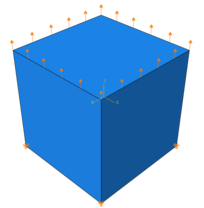
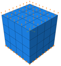
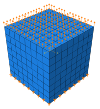
(a) Coarse mesh (200 mm)	(b) Medium mesh (50 mm)	(c) Fine mesh (25 mm)
Figure 29. Uniaxial tension example

Tabla 4. Parameters for the mesh-insensitivity verification example

Mesh	leq	fck	fcm	ftm	Gch	GF	b	ac	at	bc	bt
	(mm)	(MPa)	(MPa)	(MPa)	(N/mm)	(N/mm)
Coarse	200	25	33	2.58	22.43	0.137	0.6	7.873	1	581	5648
Medium	50	25	33	2.58	22.43	0.137	0.914	7.873	1	145.2	1412
Fine	25	25	33	2.58	22.43	0.137	0.967	7.873	1	72.6	706

Figure 30 presents the plots that constitute the major inputs for this implementation. Figure 30.a and Figure 30.b display plots of compressive/tensile stress vs. crushing/cracking strain, respectively; Figure 30.c and Figure 30.d display plots of compressive/tensile damage variable vs. crushing/cracking strain, respectively. Figure 30 shows that the inputs are strongly dependent on the mesh size; conversely, outputs are expected to be almost independent on it. Noticeably, compressive plots are displayed only for information.

(a) Compressive stress vs. crushing strain	(b) Tensile stress vs. cracking strain
(c) Compressive damage variable vs. crushing strain	(d) Tensile damage variable vs. cracking strain
Figure 30. Results of the proposed algorithm for the uniaxial tension example using coarse, medium and fine meshes

Given that the problem under consideration is extremely simple, a closed-form solution can be provided. This solution is derived from the uniaxial tensile constitutive law given by equation (57) (Figure 27.b), with the critical crack opening w_c obtained from equation (58) (w_c = 0.273 mm).

After the implementation in ABAQUS of the plots displayed in Figure 30, Figure 32 presents the force- displacement plots that are obtained for each mesh size. For comparison purposes, Figure 32 contains also the aforementioned closed-form solution. Figure 32 shows a satisfactory agreement among the plots for the three mesh sizes; this observation corroborates the mesh-insensitiveness of the proposed methodology. As well, numerical results match analytical ones, thus confirming the accuracy. Noticeably, the best match is provided by the coarse mesh; this circumstance can be explained because a single element is the closest representation of the closed-form solution. On the other hand, the result of the fine mesh is better that the one of the medium mesh; certainly, further refinements would lead to higher accuracy.

(a) Coarse mesh (200 mm)	(b) Medium mesh (50 mm)	(c) Fine mesh (25 mm)
Figure 31. Uniaxial damage localization

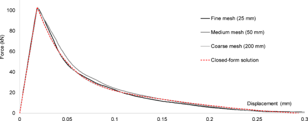
Figure 32. Force-deflection plots for the uniaxial tension example (coarse, medium and fine meshes)

The area under the plots in Figure 32 (between the peak and the displacement for zero stress in the closed-form solution) is equal to 5.5149, 5.6358 and 5.3965 Nm for coarse, medium and fine meshes, respectively. These quantities represent the fracture work; it can be converted into fracture energy per unit area (G_F) dividing by the area perpendicular to the applied displacement following the regularization method [99]; results are: 0.1379, 0.1409 and 0.1349 N/mm for coarse, medium and fine meshes, respectively. Comparison with the values indicated in Table 4 shows a satisfactory agreement.

3.6 Experimental validation of damage evolution

Accuracy and reliability of the proposed methodology are verified by simulating one experiment with the particular algorithm described in subsection ‎3.4 and with the formulation to determine the damage variables described in subsection‎3.1. The experiment [110] consisted in imposing a cyclic force law to a number of plain concrete cylinders. Figure 33 displays the imposed force law (in terms of stress).

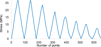
Figure 33. Input force law for the plain concrete test

This experiment had been previously simulated [80] [111]. Analog to the mesh sensitivity verification example, the proposed approach has been implemented in ABAQUS FEM program.

The simulated test refers to a cube element with 125 mm side; it is discretized with a single element. The maximum number of iterations is 2, and loading increment is 4 × 10^-4 mm. Table 5 displays the values of the parameters.

Tabla 5. Parameters for the simulation of the plain concrete test

fck (MPa)	fcm (MPa)	ftm (MPa)	Gch (N/mm)	GF (N/mm)	b	ac	at	leq (mm)	bc	bt
18	26	2.07	20.7	0.1312	0.8	7.873	1	125	310.48	2960

Figure 34 displays major outputs of the simulations, compared with the corresponding experimental results. Figure 34.a exhibits stress-strain plots and Figure 34.b shows the evolution of damage variable (d) in terms of strain. In points “▲” in Figure 34.b, the abscissa corresponds to measured values of strain and the ordinate corresponds to damage determined applying equation (23) to the experimental plots in Figure 34.a, as average for each pair of unloading and reloading branches. In the numerical plots in Figure 34.b, the horizontal segments belong to constant damage along unloading and reloading branches.

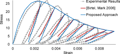
(a) Stress-strain

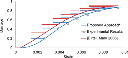
(b) Damage-strain

Figure 34. Comparison between experimental and simulated results for the plain concrete test

Figure 34.a shows a satisfactory agreement between numerical and experimental results, particularly in terms of envelope curve; noticeably, envelope results from both models are almost identical (because the same uniaxial constitutive laws have been considered). Figure 34.b shows an adequate agreement between the experimental damage (at the measured strains) and the numerical damage calculated with the proposed approach, given that points “▲” are highly close to the numerical curve.

4 Reinforcing bars modeling

4.1 Introduction

The behavior of reinforcing steel may control the response of reinforced concrete structural elements subjected to earthquake loading. Thus, it is necessary to use an appropriate model that predicts the fundamental characteristics of steel within a range of loading.

This section presents the analytical model used in this work to simulate the linear and nonlinear behavior of reinforcing bars. 2D truss finite element is used in this study to model the reinforcing bars, the model assigned to such element is used to perform the simulation of different reinforced concrete elements subjected to monotonic and cyclic loading.

4.2 Reinforcing bars models for cyclic and monotonic loading

A rate-independent elasto-plasticity model with isotropic hardening has been used for the simulation of monatomic loading, in the other hand a combined isotropic-kinematic hardening has been used for the simulation of cyclic loading. The available steel plastic models in ABAQUS [89] has been used to simulate the behavior of steel reinforcement. In these models the total stain is written in terms of elastic and plastic strain rates as:

${\overset {\cdot }{\boldsymbol {\varepsilon }}}\,={\overset {\cdot }{{\boldsymbol {\varepsilon }}^{e}}}+$${\overset {\cdot }{{\boldsymbol {\varepsilon }}^{pl}}}$

(63)

The elastic behavior follows Hook's law and is written as:

${\boldsymbol {\quad \quad \,\,}}{\overset {\cdot }{\boldsymbol {\sigma }}}=\,{\boldsymbol {D}}_{0}^{el}\,:{\overset {\cdot }{{\boldsymbol {\varepsilon }}^{e}}}=$${\boldsymbol {D}}_{0}^{el}\,:\left({\overset {\cdot }{\boldsymbol {\varepsilon }}}-{\overset {\cdot }{{\boldsymbol {\varepsilon }}^{pl}}}\right)$

(64)

${\textstyle {\boldsymbol {D}}_{0}^{el}}$ is the elastic stiffness tensor, ${\textstyle {\boldsymbol {\sigma }}}$ and ${\textstyle {\boldsymbol {\varepsilon }}}$ are the stress and strain tensors.

These models use the Von Mises yield condition with an associated plastic flow. Hence, the yield function and plastic potential are defined by the same function. The pressure-independent yield function is defined by the function

$F({\boldsymbol {\sigma }},{\boldsymbol {\alpha }})={\sqrt {{\frac {3}{2}}\left({\boldsymbol {\sigma }}^{'}-{\boldsymbol {\alpha }}^{'}\right):{\left({\boldsymbol {\sigma }}^{\boldsymbol {'}}-{\boldsymbol {\alpha }}^{'}\right)}}}\,-$$\,{\sigma }_{y}$

(65)

where σ^' and α' are the deviatoric parts of the stress and backstress tensors σ and α respectively, σ_y is the uniaxial yield stress.

As it's mentioned above, an associated plastic flow is used. Therefore, as the material yields, the inelastic deformation rate is in the direction of the normal to the yield surface and there's no volumetric plastic strains. This assumption is generally acceptable for application of reinforced concrete cyclic simulation as long as microscopic details, such as localization of plastic flow occurring as a metal component ruptures due to cyclic fatigue loads, are not of interest.

The plastic flow is given by:

${\boldsymbol {\quad \quad \,\,}}{\overset {\cdot }{{\boldsymbol {\varepsilon }}^{pl}}}=$$\,{\overset {\cdot }{\overline {\varepsilon }}}^{pl}{\frac {\partial F}{\partial {\boldsymbol {\sigma }}}}$

(66)

where ${\textstyle {\overset {\cdot }{\overline {\epsilon }}}^{pl}}$ is the equivalent plastic strain rate.

The nonlinear isotropic-kinematic hardening model is based on the work of Lemaitre and Chaboche (1990) [69]. In this model, the evolution law consists of two components; Nonlinear kinematic hardening describes the translation of the yield surface in stress space through the backstress tensor α, the isotropic hardening describes the change of the equivalent stress that defines the size of the yield surface σ⁰ as a function of plastic deformation. The nonlinear kinematic hardening component is defined to be two terms; Linear kinematic hardening and relaxation term which introduces the nonlinearity, nonlinear kinematic hardening law is defined in the next formulation:

${\overset {\cdot }{\mathit {\boldsymbol {\alpha }}}}_{}={C}_{m\,}{\frac {1}{{\sigma }_{y}}}\left({\boldsymbol {\sigma }}-\right.$$\left.{\boldsymbol {\alpha }}\right){\overset {\cdot }{\overline {\epsilon }}}^{pl}-$${\gamma }_{m\,}{\mathit {\boldsymbol {\alpha }}}_{k\,}{\overset {\cdot }{\overline {\varepsilon }}}^{pl}$

(67)

where ${\textstyle {C}_{m\,}and\,{\gamma }_{m\,}}$are material parameters that can be calibrated form cycle test data, ${\textstyle {\overset {\cdot }{\overline {\epsilon }}}^{pl}}$ is the equivalent plastic strain rate. When ${\textstyle {\gamma }_{m\,}}$is zero, the model recovers to Linear kinematic hardening.

The isotropic hardening component of the model defines the evolution of the yield surface size, this evolution can be defined by a simple exponential law

${\sigma }^{0}={\sigma }_{y}+{Q}_{\infty }\left(1-{e}^{-{b}_{m}{\overline {\varepsilon }}^{pl}}\right)$

(68)

where ${\textstyle {Q}_{\infty }\,and\,{b}_{m}\,}$ are material parameters and can be calibrated from test data.

The required data for the kinematic hardening component have been obtained from the results of stabilized cycle simulation. In this work the FEM package seismostruct [112] has been used to obtain the cyclic behavior of reinforcing bars subjected to symmetric strain cycles. A stabilized cycle is obtained by cycling a specimen over fixed strain range Δε until the stress strain curve is no longer changes from one cycle to the next. Figure 35 shows the strain stress curve for a stabilized cycle according to [89], each pair of ( ${\textstyle {\sigma }_{i},{\epsilon }_{i}^{pl})}$ is specified after shifting the strain axes to ${\textstyle {\epsilon }_{p}^{0}}$.

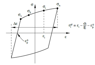
Figure 35. Stress-strain data for a stabilized cycle [89]

The shifted data are entered in tabular form in ABAQUS [89] as stress-strain, more detailed information about the calibration and the calculation of the back stresses can be found in [89].

Another possibility to simulate the nonlinear behavior of steel bars under cyclic loading is to use a linear-kinematic hardening model instead of combined hardening "isotropic and kinematic"; such model requires the hardening parameter to be defined. Hardening parameter is defined as the difference between the yield stress and higher stress value divided over the plastic strain "strain difference between the total strain correspond to the higher stress and the yield strain value".

5 Bond-slip effect modeling

5.1 Introduction

This section provides a general overview of the fundamental mechanisms governing the bond behavior between reinforcing bars and the surrounding concrete. A summary about the recent and past studies and models is also provided. Finally, a new implementation scheme is presented, this scheme is particular appropriate to implement the interface bond model developed by [20] in 3D FEM simulation.

The stress transfer capacity between concrete and reinforcing bars is generally referred as the bond of reinforcing bars. This phenomenon is an essential mechanism that engages both material generating the composite action of reinforced concrete structures. Bond of deformed bars (not plain) has been studied and characterized by large number of researchers, which has led to be well documented in design and modeling codes [113] and [114]. Transfer of forces from the reinforcement to the surrounding concrete for a deformed bar shown in Figure 36 occurs by :

• Chemical adhesion between the bar and the concrete;

• Frictional forces arising from the roughness of the interface, forces transverse to the bar surface, and relative slip between the bar and the surrounding concrete.

• Mechanical anchorage or bearing of the ribs against the concrete surface.

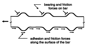
Figure 36. Source of bond resistance in a deformed bar [114]

When deformed bar moves with respect to the surrounding concrete (slip), the chemical surface adhesion is lost while bearing and friction forces are mobilized; friction forces are mobilized due to bar roughness and bearing forces at the ribs caused by the wedding action against the concrete. The pressure exerted by ribs onto concrete creates micro crack referred as Goto cracks [115] starting at the tip of the ribs and propagating transversally away from the bar as shown in Figure 37. With increasing the demand and the slip, the wedging action of the ribs tends to introduce a radial expansion at the interface, which activates the passive confinement in the concrete. Radial expansion produces a hoop expansion in the concrete, which causes splitting cracks to develop at the surface in contact with the bar and propagate radially, as shown in Figure 37. This hoop expansion is restrained by the undamaged outer concrete ring aswell as the confining reinforcement if any. For low confinement conditions, splitting cracks propagate radially through the concrete cover and the bond fails abruptly. This type of failure is referred as splitting failure and can be represented by vertical drop of the bond stress at point A in Figure 38.a, the horizontal axes in Figure 38 the is referred to the relative displacement "slip".

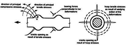
Figure 37. Goto cracks due to bond slip [114]

When sufficient confinement and cover are provided, the bond resistance will be increased due to introducing large radial stresses at the contact between the concrete and the bars. Further slip occurs after crushing the concrete front of the ribs, crushed particles of concrete contributes to increase the radial component of the bearing forces and lateral shear crack will be generated in as shown in Figure 38.b. At this point the slope of bond-slip decrease rapidly (approximately at point B in Figure 38.b). If the confinement of the concrete is not sufficient, splitting failure can happen, conversely if the concrete is well confined, higher bond strength can be achieved till reaching the maximum bond-strength at point C in Figure 38.c, at this state a part of or the total concrete keys will be crashed and sheared. Bond stress starts to decrease with increasing the slip and more concrete will be crushed, failure occurs due to loss of interlocking action caused by crushing and shearing the concrete keys between ribs. Eventually, the bar is pulled out from the concrete and only frictional resistance remains at point E in Figure 38.c, this type of failure is referred as pull-out failure. Figure 38 shows a representation of the damage evolution for pull-put failure type under monotonic loading.

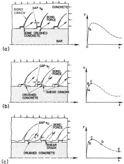
Figure 38. Monotonic bond-slip behavior for pull-out failure [116]

Bond-slip behavior and damage mechanism under cyclic loading are even more complex, the hysteretic behavior is well studied and theorized by [116] as shown in Figure 39.

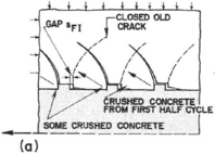
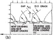
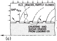
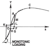
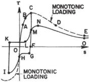
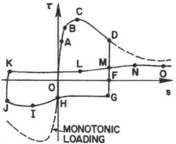
(a)	(b)	(c)
Figure 39. Cyclic bond-slip behavior for pull-out failure [116]

Cyclic behavior for low demand reversal before developing shear crack is presented in Figure 39.a. After unloading at point A along path AF, the gap between the right side of the ribs and the adjacent concrete, after concrete crushing on the left side of the ribs, remains open with a width equal to the residual slip at point F. Only a small fraction of the slip is recovered by the elastic unloading of the concrete. When the slip is reversed along path GH, some frictional resistance is built up. At H, the ribs are in contact again with the concrete but a gap has opened on the left side of the ribs. Because of a resumed contact with the concrete, a sharp increase in stiffness occurs along path HI. With increasing load, the old inclined cracks close, allowing the transfer of compressive stresses across them with no noticeable reduction in stiffness. Inclined cracks perpendicular to the old ones appear as the stress increases in this direction. At point I, a gap equal to the distance between points F and I has opened. When reversing the slip, the path IKL is similar to AFH. However, the bond resistance starts to increase again at L, when the ribs start to press broken pieces of concrete against the previous bearing face. With further movement, the transverse cracks previously closed are opened and the cracks previously opened are closed. At M, the ribs and the concrete are in full contact and the monotonic loading curve is recovered.

If the slip reversal occurs after horizontal shear cracks have initiated, a different behavior is obtained as shown Figure 39.b. When loading in the opposite direction (along path HI), the ribs press against the concrete in between whose resistance has been lowered by the shear cracks. Therefore, the bond resistance is lowered compared to the monotonic curve. When reversing the slip again (along path IKLMN), the resistance is further lowered compared to that at point I because of the additional shearing damage in the concrete. When a large slip is imposed during the first cycle, almost all the concrete between the ribs can be sheared off and the behavior will be like the one shown in Figure 39.c. When moving the bar back (along path GH), the frictional resistance is higher than that for the previous cases, in which the slip in the first cycle is smaller, because the concrete surface along the shear crack is rougher. When reloading in the opposite direction, the peak resistance (point I) is lowered. When reversing the slip again, the frictional resistance is lowered because the surface has been smoothened (path KL).

From the simulation point of view, a number of numerical models have been proposed to simulate bond-slip behavior; they can be classified depending on their scale [117].

Rib scale. The detailed geometry of the interface, including bar ribs, is modelled, concrete and steel are discretized with continuum elements [118] [119]. These models can provide very high accuracy, although with a high computational cost.

Bar scale. Ribs are not directly included in the simulation; the contact surface is idealized as smooth. Concrete and steel can be discretized with different types of elements (e.g. solid for concrete and truss or beam for steel). The interaction forces (cohesion, friction and bearing) are represented by tangential (bond) and normal stress; particular attention is usually paid to the tangential component. Bond-slip is represented through relation between bond stress and bar slip implemented in zero-thickness interface element. [120] developed a four-node zero-thickness bond-slip element to be used for two-dimensional modelling; other studies using this model have been reported. Broadly speaking, bar scale models have good balance between computational cost and ability to reproduce accurately bond behavior.

Structural Element scale. The bond-slip effects are either incorporated in the formulation of the element or taken into consideration through zero-length springs. [121] introduced the beam-column model with bond-slip proposed by [122] into the force-based fiber-section element developed by [123]. In regards to zero-length approach; [124] proposed a law to relate bar stress and slip at end of anchorage in footing-column or beam-column connections; this law has been calibrated with experimental results and used as a constitutive relation for steel fibers in a zero-length fiber-section element to simulate end rotation of RC columns. These models have low computational cost and, therefore, are suitable for simulation of full-scale structures; conversely, they do not study explicitly the bond behavior, merely reflect the additional flexibility provided by bond-slip.

Rib scale models are too computationally expensive for the practical simulation of full-scale actual structures, and element scale models can be an attractive option for large-scale simulation but cannot capture strength reduction due to bond degradation (because of slip, concrete spalling or steel yielding) and cannot be implemented in continuum elements. Bar scale models are the most appropriate for implementation in continuum elements under seismic excitation, as they represent efficiently interaction between two materials and predict different deterioration modes. A number of models of this type have been proposed:

• [Gan 2000] [125]. A double-node zero-thickness contact element is used to connect steel bar elements with the surrounding concrete. The monotonic and cyclic behavior of this element is governed by a bond-slip law originally proposed by [116] and later modified by [125] according to experimental observations. This contact element was implemented in Finite Element Code TRIX99 and used to perform 2-D cyclic analysis for shear walls.

• [Ožbolt et al. 2002] [126]. These researchers proposed a monotonic bond-slip law based on experimental results [116] and [127]. This law was implemented in the finite element code MASA using a zero-width element. Concrete and steel are discretized with solid and truss elements, respectively. This model was been verified with pull-out tests and simply-supported RC beams.

• [Lowes et al. 2004] [120]. A four-node zero-thickness bond-slip element is used for two-dimensional monotonic and cyclic modelling. The model is characterized by a normalized bond stress-slip law and a relation between the maximum bond strength and stress-strain state of concrete and steel.

• [Rabczuk et al. 2005] [128]. A 2-D two-double-node interface element, bond behavior is described in terms of radial stress-strain relation. This element was implemented in FE package ABAQUS using user subroutine; it was used in the simulation of a prestressed RC beam subjected to static load.

• [Murcia-Delso, Shing 2015a] [129]. These researchers developed a general 3-D bond-slip model accounting for bond deterioration due to cyclic slip reversals, concrete splitting, and bar yielding in tension. This model is an extension, to represent different bond deteriorations, of the semi-empirical cyclic bond-slip law proposed by [20] and [130] which is similar to that proposed by [116]. This model was implemented in a four-node zero-thickness interface element with linear shape functions and two integration points.

5.2 Spring model

This subsection describes a simple and practical model that can be used only for monotonic loading simulation. The model can be implemented in any FEM package that provides nonlinear 3D spring element with ability to define the constitutive force displacement law.

The relation between concrete and steel bars is represented by four nonlinear spring that connect the nodes of truss elements representing reinforcement bars from one side, and the nodes of 3D solid elements representing concrete material form the other side. Only the longitudinal component of bond is assigned to the springs, while the normal and rotation stiffness are ignored. Figure 40.a.b show respectively a 3D and 2D representation of the model. In Figure 40, A and B are the start and end nodes of the truss element, "Spr" refers to spring. Under well confined conditions it can be assumed to consider average "local bond" versus "local slip" relation between reinforcement and concrete, this relation can be described by bond-slip law. [90] provides detailed monotonic bond-slip law for pull-out and splitting failure as a function of bond stress τ₂ and the relative displacement S₂ as shown in Figure 41. Once the bond stress-slip relation is defined, it can be converted to force-slip law and attached to each spring as its constitutive law.

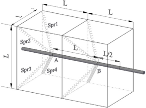
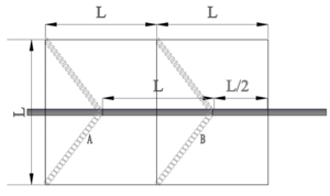
(a)	(b)
Figure 40. Implementation of Spring model for bond-slip [129]

In Figure 41; τ_f is the friction bond resistance, S_R is the distance between the bars ribs.

Bond-slip law is converted to force displacement relation and assigned as a constitutive law for the spring elements.

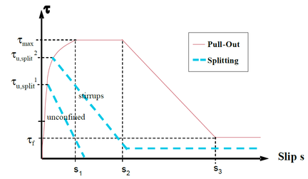
Figure 41. Monotonic bon-slip law [90]

For uniform mesh size discretization for truss and solid elements as shown in Figure 40, the force in one spring can be calculated according to Eq (69).

${F}_{bs}=\,1.36\,{D}_{b}L{\tau }_{2}$

(69)

F_bs is the equitant bond force in the spring, D_b is the bar diameter, L is the mesh size.

What makes this model useful only for monotonic loading simulation is the hardening and plasticity evolution of spring element. As was described in the general explanation of bond-slip in subsection ‎5.1, the cyclic behavior of bond stress-slip is not possible to be described by standard isotropic hardening model This might require special treatment and developing of special constitutive law to cover the nonlinear behavior of this element.

5.3 Interface model

The 3-D interface model proposed by [129] is used in this research to represent the bond relation between the longitudinal reinforcement bars and the surrounding concrete. This model is assigned to a 2-D interface element connecting steel and concrete representing a fraction of the perimeter of the bar. Their interaction is represented in the longitudinal direction by the relation between an equivalent bond stress and the bar slip. The stress-slip constitutive law uses the phenomenological law proposed by [130] which is based on concepts originally developed by [116]. This law was extensively verified by pull-out tests on bars embedded in well confined concrete.

Figure 42 displays the three components of interaction stress (σ₁, τ₂, τ₃) and relative displacement (S₁, S₂, S₃) during sliding.

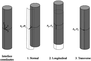
Figure 42. Stress and relative displacement components at bar-concrete interface [129]

5.3.1 Bond-stress vs slip law

The bond resistance τ₂ in the model proposed by [129] is decomposed into bearing and friction components:

${\tau }_{2}=\,{\rho }_{n}\left({\rho }_{b,s}\,\,{\rho }_{b,c\,}{\tau }_{b}+\right.$$\left.{\rho }_{f,s}\,{\rho }_{f,c\,}{\tau }_{f}\right)$

(70)

In equation (70), τ_b and τ_f are the full bearing and friction resistance of an elastic bar under monotonic pull-out action. Such resistances are multiplied by reductions factors. ρ_b,s and ρ_f,saccount for the influence of yielding of bar in tension,ρ_b,c and ρ_f,c represent the effect of slip history, and ρ_n takes into consideration splitting cracks and is a function of S₁.

Figure 43 shows the considered monotonic and cyclic bond stress versus bar slip curves. These curves are defined piecewise using polynomial functions [129] in terms of three parameters: the peak bond strength τ_max, the slip at the pick bond strength S_peak and the clear spacing between the bar ribs S_R.

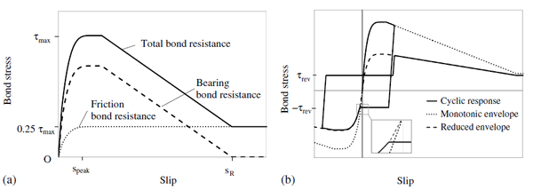
Figure 43. Bond stress-versus-slip law: (a) monotonic response; (b) cyclic response [129]

One of the main features of this model is the consideration of the reduction of bearing and friction resistance because of the diminution of the bar contact area due to yielding in tension [131] and [132]. Reduction factors that account for steel yielding in tension are expressed as follows:

${\rho }_{b,s}({\epsilon }_{s})=\left\{{\begin{matrix}1\quad \quad \quad {\rm {for}}\quad {\epsilon }_{s}\leq {\epsilon }_{y}\\{\frac {{\epsilon }_{sh}-{\epsilon }_{s}}{{\epsilon }_{sh}-{\epsilon }_{y}}}\quad \quad \,\,{\rm {for}}\quad {\epsilon }_{y}<{\epsilon }_{s}<{\epsilon }_{sh}\,\,\\0\quad \quad \quad {\rm {for}}\quad {\epsilon }_{s}>{\epsilon }_{sh}\end{matrix}}\right\}$	(71)
${\rho }_{f,s}({\epsilon }_{s})=\left\{{\begin{matrix}1\quad \quad \quad \quad \,\,{\rm {for}}\quad {\epsilon }_{s}\leq {\epsilon }_{sh}\\{\frac {{\epsilon }_{u}-{\epsilon }_{s}}{{\epsilon }_{u}-{\epsilon }_{sh}}}\quad \quad {\rm {for}}\quad {\epsilon }_{s}>{\epsilon }_{sh}\,\,\end{matrix}}\right\}$	(72)

In equations (71) and (72), ε_y, ε_sh andε_u are yielding, hardening and ultimate strains, respectively.

Reduction factors due to the slip history are given by:

${\rho }_{b,c}=1.2{\,e}^{-2.7{\left({\frac {{\overline {S}}_{max}}{{S}_{R}}}\right)}^{0.8}}\leq 1\,$	(73)
${\rho }_{f,c}=1-min\left({\frac {{S}_{max}^{+}+{S}_{max}^{-}}{{S}_{R}}},1\right)\left(1-\right.$$\left.{e}^{-0.45{\left({\frac {{S}_{cum}}{{S}_{R}}}\right)}^{0.75}}\right)$	(74)

In equations (73) and (74), ${\textstyle {S}_{max}^{+}}$ and ${\textstyle {S}_{max}^{-}}$ are the maximum absolute values of slip in positive and negative directions, respectively. ${\textstyle {S}_{cum}}$ is the cumulated slip after slip exceeds S_peak for the first time. ${\textstyle {\overline {S}}_{max}}$ is equal to:

${\overline {S}}_{max}=0.75\mathrm {max} \,\left({S}_{max}^{+},{S}_{max}^{-}\right)+$$0.25\,\left({S}_{max}^{+}+{S}_{max}^{-}\right)$

(75)

In this work, the normal displacement S₁ is assumed to be very small due to the well confined conditions in the region where it is expected that slip occurs. Therefore, the reduction factor that accounts for splitting cracks is equal to 1: ρ_n = 1.

The interface element has two additional components perpendicular to the bar longitudinal axis, one normal and one transverse tangential. The stress-displacement relations in the normal direction represent the splitting stresses introduced by the wedging action of the bar ribs. Assuming that the resultant bond force has a fixed angle of inclination of 60º as proposed in [129], the normal stress is proportional to the bond stress. For the transverse tangential direction, a penalty stiffness is introduced to restrain the rotation of the bar about its longitudinal axis.

5.4 Proposed Implementation Approach

5.4.1 General Consideration

Next subsection presents a new modeling scheme to implement the bond-slip model described in the previous subsection "developed by [129] and [133]" in a FEM analysis.

5.4.2 Modeling Scheme for Bond-Slip

The bond-slip model was originally implemented in an interface element in the FEM package ABAQUS using the user element subroutine UEL. This interface element can connect truss or beam elements representing reinforcing bars with solid elements representing surrounding concrete, as shown in Figure 44a. The modeling scheme proposed by [129] required the same discretization for steel, interface and concrete elements. This technique is efficient when longitudinal reinforcement consists of parallel bars, but can complicate the mesh when there are crossing bars with non-parallel directions. Figure 44b describes the basis of the new modeling scheme proposed herein.

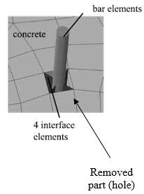
(a) Modeling scheme used in [129]	(b) Proposed modeling scheme
Figure 44. Modeling schemes with bond-slip interface model

Figure 44.b shows that the proposed technique is based on assigning, for each interface element, a pair of tie-constraint conditions; this being defined as two surfaces having the same degrees of freedom in all the contact points. The softest and stiffest surfaces are slave and master, respectively. The first tie-constraint (1) connects concrete nodes (master surface) with the interface nodes on the concrete side (slave surface). The second constrain (2) ties bar nodes (master surface) and the interface nodes on the bar side (slave surface). Hence, the relative displacement between the concrete and the bar is equal to the relative displacement at the interface element.

Figure 45 illustrates the modeling scheme for two perpendicular crossing bars. Figure 45.b and Figure 45.c show, respectively, that Bar 1 (CD) and Bar 2 (AB) are connected to four interface elements each.

(a) Two bars crossing within a solid element	(b) Four inteface elements attached to Bar 1 (CD)	(c) Four inteface elements attached to Bar 2 (AB)
Figure 45. Application of the proposed modeling scheme for two orthogonal longitudinal crossing bars

By using tie constraints, the proposed technique does not require that interface and solid elements have the same discretization. This strategy aims to overcome meshing problems and convergence difficulties. It is particularly suitable for regions with non-parallel longitudinal reinforcement bars, such as beam-column and slab-column joints, structural walls, foundations, and connections among these elements.

6. Finite element analysis verification examples

6.1 Integrating CPDM and bond-slip

In the next two subsections the proposed model is verified with large scale experiments, this involves a verification of 2D RC frames and bridge column subjected to monotonic and cyclic loading actions. CPDM described in subsection 2.4 and the proposed methodology presented in section 3 are used for the simulation of monotonic loading tests, while perfect bond conditions are assumed for such type of loading. Bond-slip model described in subsection 5.3 and its implementation scheme proposed in subsection 5.4 are implemented in the simulation of cyclic loading tests.

Bond-slip effects and damage evolution can be considered as essential issues in RC structures when they are subjected to cyclic loading. In this context, a few researchers have attempted also to integrate concrete damage-plastic behavior and bond-slip of reinforcement for practical 3-D continuum simulation of RC structures subjected to seismic loads:

• [Car et al. 2002] [60]. These researchers proposed a constitutive model based on assuming that stress transfer from concrete to steel depends on concrete damage and steel strength. Slip is represented by an irrecoverable inelastic steel strain.

• [Deaton 2013] [134]. Proposed a general model to study the 3-D cyclic behavior of non-seismic RC beam-column joints. Concrete behavior was represented by a damage model originally developed by [135] and implemented in the FE analysis program DIANA. Bond-slip was described with an interface model “line-to-solid” that follows a built-in stress-slip hysteretic law. Verifications with experimental results showed the inability of the bond model to represent the actual hysteretic behavior; concrete model showed good capacity to represent the capacity envelope but not the dissipated energy.

• [Ali et al. 2013] [136]. Studied the cyclic behavior of composed concrete–steel shear walls. The original CDPM that is implemented in ABAQUS was used to simulate concrete behavior; bond-slip is described with contact conditions. Comparison with experimental results, pointed out the lack of capturing the pinching effect (due to bond degradation and cracks opening-closing) and the strength degradation.

• [Murcia-Delso 2013] [20]. The 3-D bond-slip model was used together with the original CDPM that is implemented in ABAQUS. It is calibrated with pull-out tests and utilized to simulate 3-D cyclic behavior of RC columns supported on enlarged pile shaft foundations; satisfactory agreement was obtained. Discrete cracks were introduced at column base to simulate opening and closing of wide flexural cracks at this location and circumvent limitations of the CDPM in ABAQUS to handle the large stiffness degradation required to accurately represent cyclic response of cracks.

New smeared strategy to simulate the reclosing of cracks after tension-compression reversals is proposed in this work. As discussed in subsection 2.4 the reclosing of cracks after tension-compression reversals is governed by the parameter h_c, representing the percentage of compression stiffness recovery in the reclosed cracks. Low values of ℎ_c reduce the concrete strength after reversing; subsequently, the relative displacement between concrete and steel will be higher, thus simulating bond degradation and poor quality concrete.

In actual structures, highly uneven behavior is expected, due to the irregular distribution of bond-slip effects and to the poorer performance in the casting joints. For both reasons, in any framed structure, significantly less reclosing of cracks is expected at the member ends and the nearby segments. To enhance the opening-closing simulation of widely opened cracks in the casting joint region, [20] introduced discrete cracks at the member ends. In the current study, an alternative solution is proposed by using smaller values of h_c near the member ends. Figure 46 displays a frame modelled with different values of h_c; in the darker shadowed zones, little or no stiffness is expected upon cracks reclosing.

Figure 46. Zones of framed structures with different cracks opening-closing behavior

In practical applications, the darker shadowed areas in Figure 46 can correspond to the first and last rows of finite elements in the discretization of each column; the lighter shadowed segments can comprise the zones where bond-slip is modelled.

6.2 Simulation of monotonic loading tests

6.2.1 One floor RC frame Pires 1990

This experiment [137] is a quasi-static test consisting of imposing a displacement law to a laboratory single-span, single-story 2-D RC frame. Figure 47.b describes the tested frame, and Figure 47.a and Figure 47.c display beam and columns sections, respectively. Figure 47.b shows that both columns were loaded with constant forces and that displacement was imposed to the top left joint. Noticeably, as in the first frame test, given the absence of distributed loads on beams, there was no initial cracking.

	(a) Beam section
(b) Tested frame	(c) Column section
Figure 47. [Pires 1990] frame experiment [138] [139]

Mechanical parameters of materials are based on nominal values. The characteristic value of the concrete compressive strength is 20 MPa (C20/25, [140], and the steel yield point is 400 MPa for the longitudinal reinforcement and 500 MPa for the stirrups [141]. As described in Figure 47.c, in the critical end segments (“confinement sections”), closer stirrup spacing was used; the lengths of these segments are 40 cm in beam and 30 cm in columns. This frame had been previously simulated by [138] [139] by using concentrated and distributed plasticity models.

This test is simulated implementing the methodology of calculating the damage variables (section ‎3) in ABAQUS code [89]. Time integration follows an implicit formulation, and the global algorithm is generated by imposing energy balance. In this work, analyses are conducted for large displacements, although not for large strains. The maximum number of iterations is 10, and loading increment ranges between 0.0001 mm and 0.01 mm. Table 6 displays the selected values of the parameters. Time integration follows an implicit formulation, and the global algorithm is generated by imposing energy balance. In this work, analyses are conducted for large displacements, although not for large strains.

Tabla 6. Parameters for monotonic simulation of [Pires 1990] frame experiment

fck (MPa)	fcm (MPa)	ftm (MPa)	Gch (N/mm)	GF (N/mm)	b	ac	at	leq (mm)	bc	bt
20	28	2.222	21.12	0.133	0.9	7.873	1	25	65.48	626.67

Figure 48 displays the finite element mesh; the right part depicts steel discretization with 2-node truss elements (T3D2) and the left part describes concrete discretization with 3D 8-node hexahedron solid elements (C3D8R). Embedded element technique [142] has been used to connect reinforcing bars with the surrounding concrete assuming perfect bond conditions. Isotropic hardening has been assigned to steel material for both longitudinal and transverse bars.

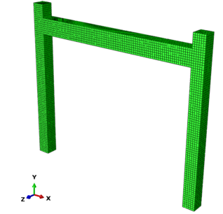
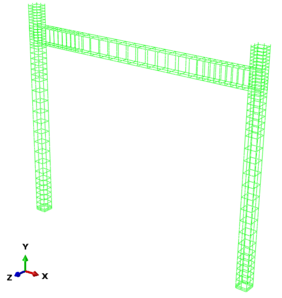
a) Initial 2D elastic domain	b) Uniaxial cyclic behavior
Figure 48. Finite element discretization of [Pires 1990] RC frame experiment

Figure 49 presents the plots that constitute the major inputs of the proposed methodology, Figure 49.a and Figure 49.b display plots of compressive/tensile stress vs. crushing/cracking strain, respectively; Figure 49.c and Figure 49.d display plots of compressive/tensile damage variable. These plots correspond to the only mesh size in the model as presented in Table 6.

For comparison results are plotted in Figure 50 together with the experimental performance. Plots from Figure 50 show that the proposed methodology captures the initial stiffness, the inception of overall yielding, maximum strength capacity, ductility phase, sequence of damage progression and the final state.

(a) Compressive stress vs. crushing strain	(b) Tensile stress vs. cracking strain
(c) Compressive damage variable vs. crushing strain	(d) Tensile damage variable vs. cracking strain
Figure 49. Major inputs of the damage variables methodology for [Pires 1990] RC frame experiment

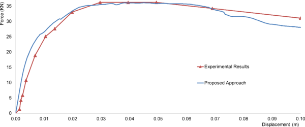
Figure 50. Experimental and simulated capacity curves for [Pires 1990] RC frame

Figure 51 shows the final damage state at the base of the right column, describing the final state and the evolution from the undamaged state. Figure 51.a and Figure 51.c represent the distribution of the compressive and tensile damage variables, respectively. Figure 51.b and Figure 51.d display, for selected finite elements, plots of such variables vs. beam displacement, respectively. Figure 51.a and Figure 51.c show that there is hinging, since both damage variables attain values close to 1. Figure 51.b and Figure 51.d show that cracking occurs for smaller displacement (approximately 20 mm) than crushing (more than 100 mm).

(a) Distribution of dc at the final state	(b) Evolution of dc
(c) Distribution of dt at the final state	(d) Evolution of dt
Figure 51. Damage at the right column base for [Pires 1990] frame experiment

Figure 51 shows that the observed phenomena are adequately reproduced by the proposed methodology, since the obtained damage distributions fit the expected results. Results from Figure 51.b.d show the rapid damage evolution in terms of top floor displacement when concrete is subjected to mainly tensile stresses in comparison to compressed side, this also fits with expected behavior and the inputs shown in Figure 49. First bars yielding under tension is detect at the top-right edge of the beam, subsequently both column at the bases, ending by yielding at top-right, bottom left edges of beam and at column bases. Compressed bars at the bases of the columns reached as well the yield stress. Figure 52.a shows the distribution of plastic stain in the longitudinal bars at the base of the right column. Figure 52.b and Figure 52.c show respectively the tension and compression stress versus the lateral displacement at the beam. The stresses values in Figure 52.b and Figure 52.c are taken as the average stress value in the highly stresses elements in the three bars shown in Figure 52.a at each side.

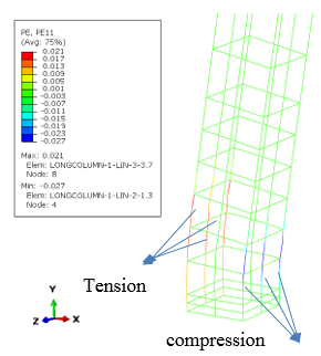
(a) Plastic strain
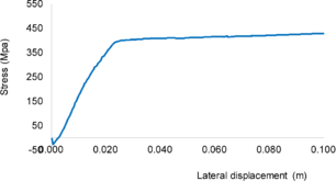
	(b) Tensile stress vs. displacement
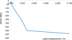
	(c) Compressive stress vs. displacement
Figure 52. Plastic strain in reinforcing bars are the right base column of [Pires 1990] experiment.

Final damaged state of the frame is demonstrated in Figure 53, compression, tension and scalar damage are presented respectively in Figure 53.a.b.c. Final stress state (KN/m²) in reinforcing bars is demonstrated in Figure 53.d

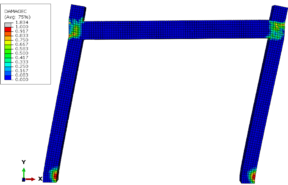
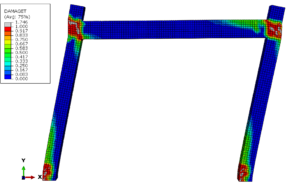
(a)	(b)
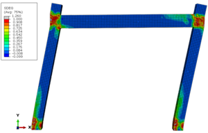
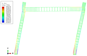
(c)	(d)
Figure 53. Final damaged state of [Pires 1990] RC frame experiment

6.2.2 Two floors RC frame [Vecchio and Emara 1990]

This experiment [143] is a quasi-static test consisting of pushing monotonically until failure a laboratory, single-span, two-story, planar RC frame. Figure 54.b and Figure 54.c display front and side views of the tested frame, respectively. Figure 54.a and Figure 54.d exhibit cross sections of columns and beams, respectively. In Figure 54 dimensions are in mm. Figure 54.b shows that both columns were loaded with constant forces, and that pushing consisted in imposing a displacement law to the top left joint. Noticeably, since there were no distributed forces acting on the beams, there was no cracking prior to the lateral pushing. The tested frame was widely instrumented, thus providing extensive information of the damage progression.

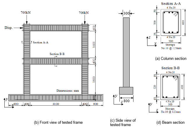
Figure 54. Frame experiment [Vecchio and Emara 1990]

Concrete mechanical parameters were determined from standard cylinder tests. The characteristic value of compressive strength is 30 MPa and the average value of secant deformation modulus is 23.67 GPa. Poisson ratio and shear deformation modulus were estimated as 0.2 and 9.86 GPa, respectively. The steel parameters were obtained from coupon tests; the stress-strain plots were approximately trilinear: an initial linear elastic branch, a horizontal yielding plateau and a plastic hardening branch. Table 7 displays the most relevant figures regarding reinforcement steel. In Table 7, bars No. 20 and 10 correspond to longitudinal and transverse reinforcement, respectively (Figure 54.a and Figure 54.d). D_b is the bar diameter, f_y / f_u are the yield point / ultimate stress, E_s is the steel modulus of elasticity, E_sh is the slope of the hardening branch, ε_sh is the strain that corresponds to the onset of hardening, and ε_u is the ultimate strain.

Table 7. Reinforcement steel parameters for the [Vecchio and Emara 1990] frame experiment

Bar No.	Db (mm)	fy (MPa)	fu (MPa)	Es (GPa)	Esh (MPa)	εsh	εu
20	19.5	418	596	192.5	3100	0.0095	0.0669
10	11.3	454	640	200	3100	0.0095	0.0695

Figure 55 summarizes the results of the experiment. Figure 55.a displays plots of pushing force vs. top level displacement. The first observed damage was flexural cracking at the end sections of the first level beam, for force 52.5 kN and displacement 2 mm; this instant can be considered as the overall yield point, since, after that point, the capacity curve became nonlinear. Under force 145 kN and displacement 9.3 mm, flexural cracks were perceived at the columns bases, and shear cracks were simultaneously detected at the first story beam. When force reached 264 kN and displacement 26.4 mm, first steel yielding was perceived in the bottom tensioned longitudinal reinforcement of the left end section of the first story beam; for force 287 kN and displacement 31.6 mm, the top tensioned longitudinal reinforcement of the right end section of the first story beam also yielded. For force 323 kN and displacement 52.5 mm, the longitudinal reinforcements of the column bases yielded as well, and hinges at the ends of the first story beam failed; this failure involved yielding of longitudinal reinforcement, and crushing of compressed concrete. Then, for force 329 kN and displacement 74.7 mm, similar failure was apparent at the column bases. Almost simultaneously, same failure affected at ends of second story beam. Afterwards, lateral stiffness was almost non-existent; therefore, collapse mechanism consisted in formation of six hinges. The experiment was terminated, for pushing force 332 kN and lateral displacement 150 mm, due to stroke limitations of the actuator, see Figure 55.a. Figure 55.b and Figure 55.c display images of the damaged bottom section of the right column, and the top left connection, respectively.

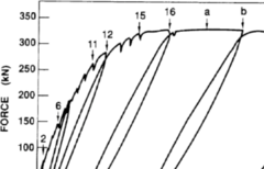
(a) Force-displacement plot	(b) Right column base	(c) Top left connection
Figure 55. Results of [Vecchio and Emara 1990] frame experiment [143]

The main objective of this experiment was to investigate the influence of shear-related effects in the overall structural behavior; the results showed that approximately 20% of the nonlinear lateral displacement was due to shear effects. Noticeably, at failure, around 12% of the overturning moment was due to P-Δ effects. Supplementary information regarding this experiment is available in [144].

This test had been previously simulated by some of the authors of this work [145] [146] [147], and by other researchers [148]. [145], used a viscous damage model, which was implemented in a fiber model with Timoshenko frame elements. [146] [147], implemented a damage plasticity formulation in a finite element model with planar 2D elements. [148], employed commercial software packages and an ad-hoc fiber model developed at University of Toronto.

Analogously to the simulated experiment in the previous subsection ‎6.2.1, this test is simulated implementing the damage evolution algorithm in ABAQUS code [89]. The maximum number of iterations is 10, and loading increment ranges between 10^-11 mm and 0.01 mm. Table 8 displays the selected values of parameters. Figure 56 displays the finite element mesh; the right side depicts steel discretization with 2-node truss elements (T3D2) and the left side describes concrete discretization with 3D 8-node hexahedron solid elements (C3D8R).Perfect bond is also assumed between concrete and reinforcing bars.

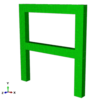
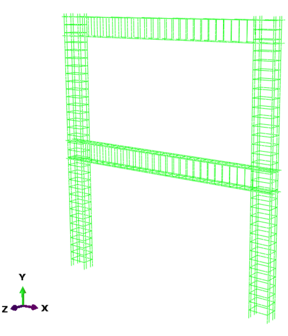
Figure 56. Finite element discretization of [Vecchio and Emara 1990] RC frame experiment

Table 8. Parameters for simulation [Vecchio and Emara 1990] frame experiment

fck (MPa)	fcm (MPa)	ftm (MPa)	Gch (N/mm)	GF (N/mm)	b	ac	at	leq (mm)	bc	bt
30	38	2.912	23.93	0.1405	0.75	7.873	1	50	156.83	1554.54

Figure 57.a displays plots of ratio ${\textstyle {\epsilon }_{c}^{pl}\,/\,{\epsilon }_{c}^{ch}}$ vs. ${\textstyle {\,\epsilon }_{c}^{ch}}$ (refer to section ‎3); Figure 57.b displays analogous plots for the tensile behavior. Figure 57 highlights that, in the proposed methodology, damage and plastic energy absorptions are not related, since ratios ${\textstyle {\epsilon }_{c}^{pl}\,/{\,\epsilon }_{c}^{ch}}$ and ${\textstyle {\epsilon }_{t}^{pl}\,/{\,\epsilon }_{t}^{ck}}$ do not approach zero when damage variables d_c and d_t are close to 1. Figure 57.a shows that the average value of ratio b (equation (56)) is approximately 0.75 (Table 8).

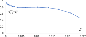
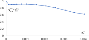
(a) Compression	(b) Tension
Figure 57. Variation of ratio between plastic and crushing / cracking strains for [Vecchio and Emara 1990] experiment

Figure 58 displays experimental results (Figure 55.a) plotted together with numerical results obtained with the proposed methodology. Descriptions of observed damage states are also displayed.

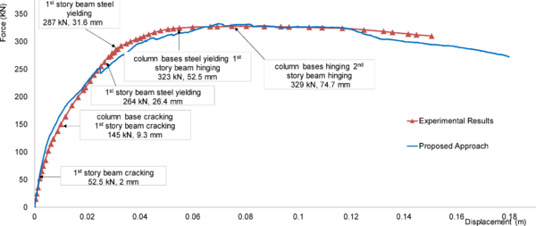
Figure 58. Experimental and simulated capacity curves for [Vecchio and Emara 1990] frame experiment

Plots from Figure 58 show the superior ability of the proposed methodology to reproduce the experimental results along the whole displacement range. It captures the initial stiffness, the onset of overall yielding, ductility phase and the sequence of damage progression and the final state. Noticeably, “overall yielding” does not refer to steel yielding but to inception of overall nonlinear behavior, due to cracking of tensioned concrete.

(a) Distribution of dt at the first story right beam-column connection	(b) Distribution of dt at the frame
Figure 59. Tensile damage variable for force 52.5 kN and displacement 2 mm for [Vecchio and Emara 1990] frame experiment

To further highlight the capacity of the proposed methodology to capture damage progression, Figure 59 through Figure 61 display the damage predicted for some of the previously described stages. Figure 59 displays the distribution of the tensile damage variable for force 52.5 kN and top level displacement 2 mm; it corresponds to the first cracking at end sections of 1^st story beam. Figure 59.a and Figure 59.b refer to the first story right beam-column connection and to the overall frame, respectively. Figure 59.a shows that cracking (indicated with lighter gray) actually occurred in the top part of beam, since the tensile damage variable reaches values close to one. Figure 59.b shows that the overall distribution of cracking fits the expected pattern according to structural analysis principles, with onset of cracking in the bottom part of the first story right beam-column connection. Figure 60 and Figure 61 refer to the final damaged state, distributions of the scalar damage variable (d) for the right column base and the top left beam-column connection are shown respectively in Figure 60.a.b.

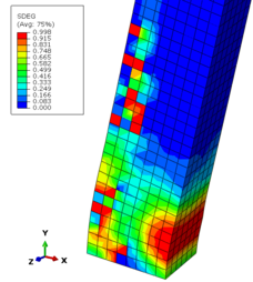
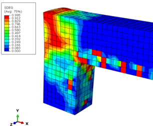
(a) Right column base	(b) Top left connection
Figure 60. Distribution of d at the final state of [Vecchio and Emara 1990] frame experiment

(a) Distribution of dc at the final state	(b) Evolution of dc
(c) Distribution of dt at the final state	(d) Evolution of dt
Figure 61. Damage at the right column base [Vecchio and Emara 1990] frame experiment

Figure 61 refers to the right column base, describing both the final state and the evolution from the undamaged state. Figure 61.a and Figure 61.c represent the distribution of the compressive and tensile damage variables, respectively; Figure 61.b and Figure 61.d display, for selected finite elements, plots of such variables vs. top level displacement, respectively. In all the images, higher damage corresponds to lighter grey. Figure 60 and Figure 61 show that the observed phenomena are adequately reproduced by the proposed methodology, since the obtained damage distributions fit the expected results. Comparison between Figure 60.a and the observed damage in Figure 55.b shows a satisfactory fit, since cracking and crushing are detected by the obtained higher values of d. Comparison between Figure 60.b and the observed damage in Figure 55.c shows also a satisfactory match. Figure 61.a and Figure 61.c show that there is hinging, since both damage variables attain values close to 1; this circumstance is observed in Figure 55.b. Figure 61.b and Figure 61.d show that cracking occurs for smaller displacement (approximately 10 mm) than crushing (more than 150 mm).

Final damaged state of the frame is demonstrated in Figure 62, compression, tension and scalar damage are presented respectively in Figure 62.a.b.c. Final stress state in reinforcing (KN/m²) bars is demonstrated in Figure 62.d

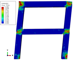
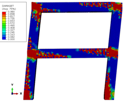
(a)	(b)
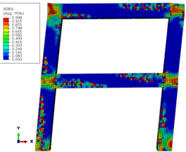
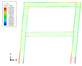
(c)	(d)
Figure 62. Final damaged state of [Vecchio and Emara 1990] frame experiment

6.3 Simulation of Cyclic loading tests

6.3.1 Bridge column [Tanaka 1990]

Several RC columns have been tested by [Tanaka 1990] [149] to study the effect of lateral confinement on their ductility. Main differences are the type of transverse reinforcement, its anchorage detailing, the axial force, and the mechanical and geometric parameters. Column unit 6 [149] has been analyzed with the proposed model. Figure 63 describes the tested column and the experimental mockup.

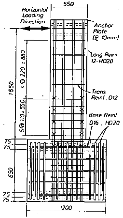
(b) Vertical section
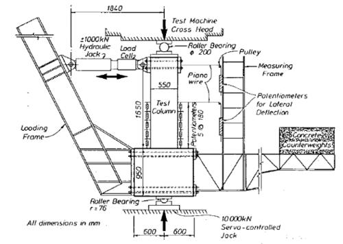
	(a) Loading arrangements
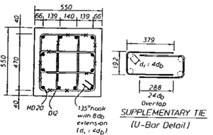
	(c) Horizontal section
Figure 63. Experiment on [Tanaka 1990] bridge column [98]

Figure 63.b and Figure 63.c display the geometry of the column, dimensions are in mm. The column was loaded with constant force 0.1 f’_c/A_g and a cyclic lateral displacement protocol was imposed by hydraulic jacks as shown in Figure 63.a. Concrete mechanical parameters were determined from standard cylinder tests. The characteristic value of compressive strength is 32 MPa and the average value of secant deformation modulus is 27.65 GPa; Poisson ratio and shear deformation modulus were estimated as 0.2 and 11.52 GPa, respectively. Steel parameters were obtained from coupon tests. Table 9 displays the most relevant information regarding reinforcement steel. In Table 9, bars HD20 and D12 correspond to longitudinal and transverse reinforcement, respectively. D_b is bar diameter, f_y / f_u are yield point / ultimate stress, E_s is modulus of elasticity, ε_sh is the strain corresponding to onset of hardening, and ε_u is ultimate strain.

Tabla 9. Reinforcement steel parameters for [Tanaka 1990] bridge column

Bar Id.	Db (mm)	fy (MPa)	fu (MPa)	Es (GPa)	εsh	εu
HD20	20	511	675	200	0.0165	0.14
D12	12	325	429	200	0.015	0.14

Figure 64 displays the imposed displacement law.

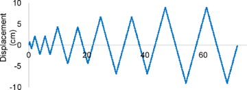
Figure 64. Imposed displacement law for [Tanaka 1990] bridge column experiment

The results of the experiment showed stable hysteretic behavior, good energy dissipation and limited strength reduction up to the final stage. Substantial crushing of compressed cover concrete (spalling) was first observed near peak load during the first cycle. During the final stage, the visible damage was concrete crushing and slight buckling of longitudinal reinforcement bars.

Figure 65 depicts the element discretization. Figure 65.a describes the concrete discretization with 3-D 8-node hexahedron solid elements (C3-D8R). Figure 65.b and Figure 65.c represent the steel and interface elements; steel is discretized with 2-node truss elements (T3-D2). Bond-slip effect is considered for the column longitudinal bars at the base of the column and development region in the footing, as shown in Figure 65.b; full bond conditions are assumed for the other segments of longitudinal bars as well as for transverse reinforcement because minimal bar slip is expected for these bars.

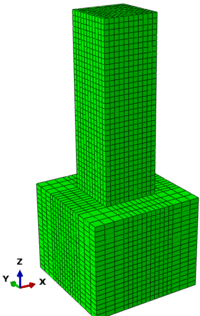
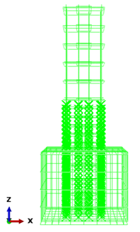
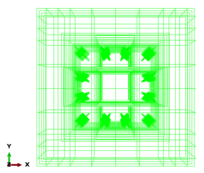
(a) Column discretization	(b) Steel and interface elements	(c) Plan view of steel and interface elements
Figure 65. Finite element discretization of [Tanaka 1990] bridge column

Steel behavior is described with a classical plastic model; isotropic hardening is used for stirrups, and nonlinear isotropic/kinematic hardening for longitudinal bars. Concrete behavior is simulated by implementing the methodology described section ‎3 in ABAQUS code [89].

Figure 66.a displays plots of ratio ${\textstyle {\epsilon }_{c}^{pl}\,/\,{\epsilon }_{c}^{ch}}$ vs. ${\textstyle {\,\epsilon }_{c}^{ch}}$, where ${\textstyle {\epsilon }_{c}^{pl}}$ refers to plastic compressive strain. Figure 66.b displays analogous plots for the tensile behavior ( ${\textstyle {\epsilon }_{t}^{pl}\,/\,{\epsilon }_{t}^{ck}}$ vs. ${\textstyle {\,\epsilon }_{t}^{ck}}$).

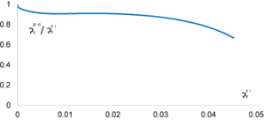
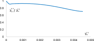
(a) Compression	(b) Tension
Figure 66. Variation of ratios plastic and crushing / cracking strains for [Tanaka 1990] bridge column experiment

Figure 66.a points out that the average of ${\textstyle {\epsilon }_{c}^{pl}\,/\,{\epsilon }_{c}^{ch}}$ is approximately equal to 0.88; this magnitude is termed b and is a required parameter in the implementation of the algorithm [150]. Table 10 displays the considered values of the parameters.

Tabla 10. Límites mínimos y máximos de riesgos de las funciones de trasformación utilizadas

fck (MPa)	fcm (MPa)	ftm (MPa)	Gch (N/mm)	GF (N/mm)	b	ac	at	leq (mm)	bc	bt
24	32	2.51	22.14	0.136	0.889	7.873	1	50	142.65	1381.74

Figure 67 displays comparisons between experimental and numerical hysteresis loops calculated with the proposed model. In Figure 67.a, the numerical results are obtained by using h_c = 0.9 in all the body, and generating a discrete crack at the footing-column interface; normal friction contact condition is assumed at that interface. In Figure 67.b, the approach to represent concrete discontinuity described in subsection ‎6.1 is applied by assigning ℎ_c = 0.01 to the first row of elements above the footing, ℎ_c = 0.1 to the elements where bond-slip is considered (Figure 65.b), and ℎ_c = 0.9 for the rest of the model (Figure 46). These values have been selected to provide the best fit with the experiment.

(a) Experiment and proposed formulation with a discrete crack	(b) Experiment and proposed formulation with reduced ℎc (subsection 6.1)
Figure 67. Experimental and numerical force-displacement response of [Tanaka 1990] bridge column experiment

Figure 67 shows that the proposed model provides a satisfactory agreement with test results, capturing initial stiffness, strength and stiffness degradation, and pinching. Plots from Figure 67.a show that the model with discrete crack is able to reproduce the main aspects of cyclic behavior; the analysis ended prematurely due to the large nonlinearity and the important separation between both blocks. The model with reduced ℎ_c (Figure 67.b) captured suitably the dissipated energy from the experiment with difference 1.66 %; conversely, the model with discrete crack (Figure 67.a) overestimated that energy by 22.88 %.

Figure 68 displays comparisons between pairs of plots obtained by numerical simulation with the proposed model and with a similar model assuming perfect bond between the reinforcement and the surrounding concrete. In Figure 68.a a discrete crack is introduced in the proposed model (as in Figure 67.a), and in Figure 68.b reduced values of ℎ_c are considered (as in Figure 67.b).

(a) Proposed formulation with a discrete crack vs. perfect bond	(b) Proposed formulation with reduced ℎc (subsection 6.1)
Figure 68. Numerical force-displacement response of [Tanaka 1990] bridge column experiment

Figure 68 highlights the relevance of bond-slip. Comparison between Figure 68.a and Figure 68.b shows that differences are more significant in the smeared model. The discrete crack model response in Figure 68.a exhibits some pinching due to the added flexibility at the column bottom; conversely, the smeared model response in Figure 68.b shows higher energy dissipation.

Figure 69 shows the experimental results plotted together with the ones obtained from the models assuming perfect bond, plots show that models with perfect bond reproduce satisfactorily the envelope behavior but lack to capture the unloading and reloading branches.

(a) Experiment vs. Perfect bond proposed formulation with a discrete crack	(b) Experiment vs. Perfect bond proposed formulation model with reduced ℎc (subsection 6.1)
Figure 69. Numerical force-displacement response of [Tanaka 1990] bridge column

Experimental observations revealed buckling in the longitudinal reinforcement bars at column bottom [149]. Figure 70 presents numerical (Figure 70.a and Figure 70.b) and experimental (Figure 70.c) representations of this failure. Figure 70.a displays the buckling that is detected at the last cycle, Figure 70.b shows the final damage state and Figure 70.c depicts the observed damage. Comparison between numerical and experimental results highlights the accuracy of the proposed formulation.

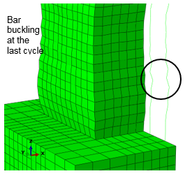
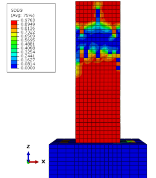
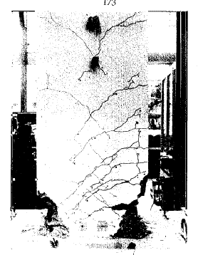
(a) Buckling in the longitudinal bars	(b) Final damage state	(c) Final state [149]
Figure 70. Final state of the bridge column

The average stress-vertical displacement behavior of the bottom-left corner longitudinal bars presented in Figure 65.c is shown in Figure 71. The average stress-displacement along embedded part of the bar inside the footing is shown in Figure 71.a, while the average stress- displacement along the region where interface elements are assigning (Figure 65) is shown in Figure 71.b. Plots from Figure 71 shown the significant influnce of introducing the bond-slip elemnts in comparision with perfect bond model on the hesteritic behavior of stress-displacment in longitudinal bars. The higher negative displacement in the hysteretic behavior of the model with bond-element shown in Figure 65, can be understood as a result of penetration due to bond degradation.

(a) Proposed formulation with reduced ℎc (subsection 6.1) vs. perfect bond along 55 cm	(b) Proposed formulation with reduced ℎc (subsection 6.1) vs. perfect bond along 130 cm
Figure 71. Numerical results of stress-slip relation in the reinforcing bars for [Tanaka 1990] bridge column experiment

The average cyclic damage evolution at the bottom of the column with depth 50 cm (See Figure 73) is presented in Figure 72. Plots in Figure 72 are obtained from the proposed model with reduced h_c (subsection ‎6.1). Plots from Figure 72 show the evolution of the compressive, tensile and scalar damage along the entire range of loading. It can be seen that the scalar damage follows mainly the tensile damage at a certain value, subsequent, the value of the scalar damage exceeds the tensile one and rises up as long as the compressive damage is increasing. This results holds true for a low value of h_c in the considered zone, as well low value of r* as it’s explained in subsection ‎2.4, equations (24) (25) (26).

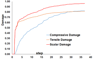
Figure 72. Cyclic damage evolution of [Tanaka 1990] bridge column experiment, proposed formulation with reduced ℎc (subsection 6.1)

Same plots from Figure 72 are plotted versus top lateral displacement in Figure 73.b.c.d for compressive, tensile and scalar damage respectively. Plots from Figure 73 confirm the expected results, in which the damage variables, as well the scalar damage increase along increasing the displacement, as well as, when at the last two cycles for constant value of displacement (see Figure 64)

(a) Cinsidered zone for damage evolution	(b) Compressive damage evolution
(c) Tensile damage evolution	(d) Scalar damage evolution
Figure 73. Cyclic damage evolution vs. top displacement of [Tanaka 1990] bridge column experiment, proposed formulation with reduced ℎc (subsection 6.1)

6.3.2 Building frame [Pires 1990]

The experiment presented subsection ‎6.2.1 and initially was simulated for monotonic loading, is further studied and simulated again under cycle loading. The RC frame is subjected to cyclic displacement law in Figure 74, this displacement is imposed at the beam side. Mechanical parameters of materials as well as the geometry of the frame are presented in subsection ‎6.2.1.

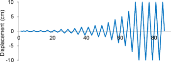
Figure 74. Imposed cyclic displacement law for [Pires 1990] frame experiment

Analogously to bridge column experiment (subsection ‎6.2.1), this test is simulated by implementing the damage variables algorithm [129] in ABAQUS code and the interface bond-slip model described in ‎5.3, modeling schemes described in subsections ‎5.4 and ‎6.1 are also incorporated. The model has been refined to implement the bond-slip elements in the foundation. Table 6 displays the calculated values for the parameters of the damage variables methodology.

Table 11. Parameters for monotonic simulation of [Pires 1990] frame experiment

fck (MPa)	fcm (MPa)	ftm (MPa)	Gch (N/mm)	GF (N/mm)	b	ac	at	leq (mm)	bc	bt
20	28	2.222	21.12	0.133	0.97	7.873	1	21.6	56.57	541.45
20	28	2.222	21.12	0.133	0.94	7.873	1	37	96.91	927.48

This experiment is simulated using bond-slip elements where bars are expected to slip. Figure 75 displays the frame discretization; Figure 75.a shows the overall discretization, Figure 75.b presents a general view of steel elements, Figure 76.a shows the discretization of interface element "bond-slip element" attached to longitudinal bars, Figure 76.b depicts a more detailed view of the right beam-column joint steel bars, and Figure 76.c shows the same of Figure 76.b with bond-slip element, Figure 76.d depicts a closer view of the right column base.

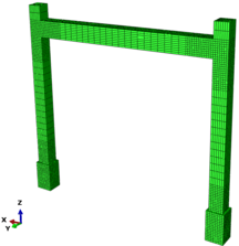
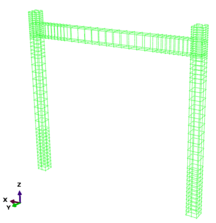
(a) Frame discretization	(b) Steel elements discretization
Figure 75. Finite element discretization of [Pires 1990] frame experiment

As shown in Figure 76.a, bond-slip elements are assigned to the longitudinal bars along the column foundation, inside beam-column joints, at the column top and bottom ends, and at beam-ends. Noticeably, the proposed modeling scheme (subsection ‎5.4) allows that bar elements intersect in the same solid element without need to generate perpendicular holes nor to use double nodes. Regarding the approach described in subsection ‎6.1, similarly to Figure 46, ℎ_c = 0.01 for the bottom and top row of elements inside the columns; then, ℎ_c = 0.1 for the elements where bond-slip is considered (Figure 76), and ℎ_c = 0.9 for the rest of the model. The results from this approach are compared with those after introducing discrete cracks right above the footings.

(a) Steel and interface elements	(b) Steel element at right beam-column joint
(c) Interface elements at the right beam-column joint	(d) Interfce elements at the right column base
Figure 76. Bond-slip elements discretization of [Pires 1990] frame experiment

Analogously to Figure 67, Figure 77 displays comparisons between experimental and numerical hysteresis loops obtained with the proposed model. Plots from Figure 77 provide similar conclusions than Figure 67.

(a) Experiment and proposed formulation with a discrete crack	(b) Experiment and proposed formulation with reduced ℎc (subsection 6.1)
Figure 77. Experimental and numerical force-displacement response of [Pires 1990] frame experiment

Similarly to Figure 68, Figure 78 displays comparisons between numerical hysteresis loops obtained with the proposed model and assuming perfect bond. Figure 78 allows deriving parallel observations than Figure 68.

(a) Proposed formulation with a discrete crack vs. perfect bond	(b) Proposed formulation with reduced ℎc (subsection 6.1) vs. perfect bond
Figure 78. Numerical force-displacement response of the frame experiment

(a) Experiment vs. Perfect bond proposed formulation with a discrete crack	(b) Experiment vs. Perfect bond proposed formulation model with reduced ℎc (subsection 6.1)
Figure 79. Numerical force-displacement response of [Pires 1990] frame experiment

Figure 99 display similar comparison as shown in Figure 69, derived observation are also similar. Final state in terms of tensile, compressive, and total damage is represented in Figure 80, results from Figure 80 show that the damage is mainly localized at the top and bottom of the column, as well in the joints. This can be explained by the small sections of column in comparison with the beam section, also since the beam is not loaded by any vertical load before applying the lateral displacement conversely to the columns.

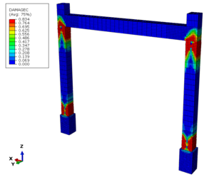
(a) Compressive damage

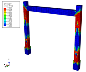
(b) Tensile damage

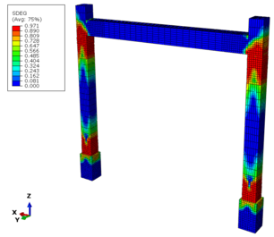
(c) Scalar damage

Figure 80. Final damage state, proposed formulation with reduced ℎc (subsection 6.1) of [Pires 1990] frame experiment

Similarly to Figure 72, the average cyclic damage evolution at the bottom of the column with depth 30 cm is presented in Figure 81. Plots in Figure 72 are obtained from the proposed model with reduced h_c (subsection ‎6.1). Plots from Figure 81 show the evolution of the compressive, tensile and scalar damage along the entire range of loading. Similar results to Figure 72 can be derived from plots in Figure 81

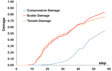
Figure 81. Cyclic damage evolution of [Pires 1990] frame experiment, proposed formulation with reduced ℎc (subsection 6.1), bottom of column

Same plots from Figure 81 are plotted versus top lateral displacement in Figure 82.b.c.d for compressive, tensile and scalar damage respectively. Plots from Figure 82confirm again the expected results, in which the damage increases along the last five cycles at a constant displacement value (see Figure 74).

(a) Cinsidered zone for damage evolution	(b) Compressive damage evolution
(c) Tensile damage evolution	(d) Scalar damage evolution
Figure 82. Cyclic damage evolution vs. top displacement of [Pires 1990] frame experiment, proposed formulation with reduced ℎc (subsection 6.1), bottom of column

Similar plots to the ones in Figure 81 and Figure 82 are presented in the next figures for the average damage evolution at top part of the column, and at the beam column joint. Same results can be derived.

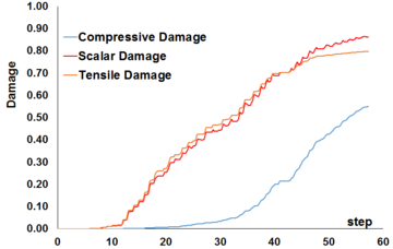
Figure 83. Cyclic damage evolution of [Pires 1990] frame experiment, proposed formulation with reduced ℎc (subsection 6.1), top of column

(a) Cinsidered zone for damage evolution	(b) Compressive damage evolution
(c) Tensile damage evolution	(d) Scalar damage evolution
Figure 84. Cyclic damage evolution vs. top displacement of [Pires 1990] frame experiment, proposed formulation with reduced ℎc (subsection 6.1), top of colum

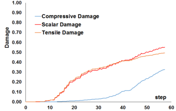
Figure 85. Cyclic damage evolution of [Pires 1990] frame experiment, proposed formulation with reduced ℎc (subsection 6.1), beam column joint

(a) Cinsidered zone for damage evolution	(b) Compressive damage evolution
(c) Tensile damage evolution	(d) Scalar damage evolution
Figure 86. Cyclic damage evolution vs. top displacement of [Pires 1990] frame experiment, proposed formulation with reduced ℎc (subsection 6.1), beam column joint

7 Continuum mechanics-based approaches concluding remarks

A new methodology to calculate damage variables "damage evolution" for Concrete Plastic Damage Models has been proposed, the methodology is suitable to simulate the monotonic and cyclic behavior of reinforced concrete structures.

The proposed methodology is mesh-insensitive, is based on a sound continuum mechanics formulation, and does not require calibration with experimental results. Implementation is straightforward. A particular algorithm is presented to implement the methodology in the CPDM of FEM software ABAQUS. Mesh-insensitivity is validated in a simple tension example. Accuracy and reliability of the proposed methodology are verified by simulating a cyclic loading experiment on plain concrete specimens, the methodology has been verified as well by simulating large scale tests consist in pushing monotonically and cyclically until failure different RC structures. Following the main verification conclusions:

Tension example. This example confirms the mesh-insensitiveness of the proposed methodology. As well, numerical results match analytical ones, thus ratifying their accuracy.

Cyclic experiment on plain concrete. The simulation of the cyclic experiment on plain concrete corroborates the capacity of the proposed approach to reproduce damage evolution and stress-strain behavior, both in terms of envelope curve and stiffness degradation at each unloading / reloading cycle. Agreement between experimental and numerical damage at measured strain levels is satisfactory.

Validation with Experiments-Monotonic loading: Two RC frames have been simulated, results have proved the ability of the proposed methodology to reproduce accurately the experimental force-displacement results along the whole displacement range. Captures initial stiffness, onset of the overall yielding, sequence of the damage progression, collapse mechanism, and final state. All failure and degradation modes are adequately simulated: tensioned concrete cracking, compressed concrete crushing, and reinforcement steel yielding.

Aforementioned work has been extended to study the cyclic behavior of RC structures. In this context, an integrated continuum FEM model is proposed for monotonic and cyclic simulation of RC frames. The model combines the methodology proposed for calculating the damage variables of CPDM and the 3-D interface bond-slip model developed by [20]. A new technique to integrate the interface model in a continuum FEM model of regions with crossing bars is presented. The proposed model is used to simulate two experiments consisting in imposing cyclic displacement laws to an RC column and a frame. These experiments are also simulated with the same model although assuming perfect bond conditions.

Validation with Experiments-Cyclic loading: Obtained results of simulating the cyclic behavior of one RC bridge column and one RC building frame, show that the proposed model is able to predict the actual behavior of highly damaged RC elements and frames, capturing strength reduction, stiffness degradation and pinching. Noticeably, this model uses only a reduced number of parameters and does not require any calibration with experimental results. Comparison with the results obtained assuming perfect bond points out the high relevance of bond-slip in the hysteretic behavior and the energy dissipation capacity.

The proposed integrated model can constitute a practical tool for accurate simulation of highly damaged medium-size RC structures, both in research and in conventional analyses. It can be also used to calibrate more simplified models.

PART II-STRUCTURAL COMPONENT-BASED APPROACHES

1 Introduction and motivation

The purpose of developing Part II is; First, investigate the capacity of the simplified numerical models and commonly used in earthquake engineering. Second, although the advanced model developed in Part I showed satisfactory performance, its high computational cost raises the need to develop a model that can capture the overall response with lower cost.

As discussed in the general introduction of this dissertation, numerical models can be divided into two main groups according to their formulation to describe the nonlinear behavior of structures. Part I dealt with complex models that are based on continuum mechanics-based approaches, this implied that structural components (e.g. columns, beams, walls) are discretized to many micro finite elements. Reinforced concrete elements are simulated by combining two materials, concrete simulated by solid elements while steel bars are described by truss bars, each is associated to a constitutive material model, relation between concrete and steel elements is described as well by a continuum model. Part II will deal with more simple models that are based on structural approaches. In other words, the models discussed in this part are derived from simplified theories of mechanics of material, structural components can be discretized with simple finite elements models (e.g. flexural bar element for column and beams). The composite material behavior is not described explicitly, rather the used element in these models aims to describe the response of the complete structural component. Different sources of degradation are also described, either by the element directly or by attaching specific element in the locations where the damage is expected to occur. These models are referred in this work as structural component-based models.

It can be distinguished between two type of structural component-based models according to the distribution of plasticity. These models are named as lumped and distributed models. Lumped plasticity models assume that the plastic deformation will be concentrated at one point along the length of the element, while distributed plasticity models provide more accuracy by capturing the plastic deformations along a specific plastic hinge length of at different locations along the element length and at different points at the cross section of the element. The lumped plasticity approach is advantageous due to its computational efficiency and for its analogy to simple elasto-plastic analysis procedures used in design practice. The distributed plasticity approach, however, is convenient for performance based design since it has the ability to capture local behaviors at intermediate element lengths and takes the spread of plasticity along an element length into account. Both approaches are discussed in the following sections, their capacity is verified by simulating the experiments described in the previous part of this dissertation.

After verifying the commonly used structural component-based models in earthquake engineering, a numerical study is conducted on the relation among the non-simulated deterioration modes of the elements of non-ductile RC frames and their final capacity.

The main contribution of this part is developing an advanced structural component-based model for simulating the nonlinear dynamic behavior of old reinforced structures, accounting for flexure, shear and axial deterioration modes. The capacity of the developed model is verified by simulating the nonlinear dynamic behavior of an existing non-ductile building and the prototype building.

2 Models for nonlinear analysis

2.1 Lumped plasticity models

The lumped plasticity approach utilizes the simplicity of the plastic hinge concept by separating a line element into elastic and inelastic components. A fixed point "zero length element" or predetermined length (typically the plastic hinge length), is determined to be the region in which all inelastic action is concentrated, while elastic properties are assigned to the remainder of the element. The inelastic behavior in the plastic hinge is determined from a sectional analysis of the critical section, which has detailed description of the geometry and material properties (uniaxial constitutive models) assigned to sections within this region. Uniaxial constitutive material models for both steel and concrete is defined and assigned to the corresponding components of a discretized section. This section is then assigned to the plastic hinge(s) of the element. Determining the section’s behavior usually requires a sectional analysis to be completed first, and then the moment-curvature relationship is assigned to the plastic hinge(s) to determine the element response under external loads. Other methods define a backbone curve (capacity curve), such methods are acceptable when the element behavior is previously well known and does not require the initial sectional analysis.

The first inelastic concentrated plasticity model was proposed by Clought et al in 1965. [151] shown in Figure 87.a. In this model, known as the two-component model, a bilinear elastic-strain hardening moment-curvature relationship is assumed along the length of the element. The beam model consists of two components acting in parallel: one which is linear elastic and one which is elastic-perfectly plastic with the plastic deformations concentrated in plastic hinges at the ends of the element. The elastic modulus of the linear component is equal to the strain hardening modulus p ⋅ EI of the moment-curvature relation, where EI is the pre-yield section stiffness. The elastic modulus of the elasto-plastic component is equal to q ⋅ EI where q = 1− p. One of the shortcomings of this model is the difficulty of accounting for the stiffness deterioration of RC elements during cyclic load reversals.

To overcome the problem of stiffness deterioration, Giberson proposed another model in 1967 [152] . This model is known as the one-component model shown in Figure 87.b . It consists of two nonlinear rotational springs which are attached at the ends of a perfectly elastic element representing the girder. All nonlinear deformations of the girder element are lumped in the two rotational springs. This is a simplification of experimental evidence which shows that inelastic deformations spread over a finite region at the ends of the girder. Giberson's model has the advantage that any kind of hysteretic law can be assigned to the nonlinear springs. This fact along with the simplicity of the model accounts for its wide use in analytical studies to date.

To describe the cyclic behavior of nonlinear spring, a hysteretic law is needed. The first model was proposed by [151] and a more refined model was Takeda et.al 1970 [153]. After this, Takeda's model has been widely used in the description of the hysteretic moment curvature or moment-rotation relation of RC members.

The concentrated plasticity concept was generalized to incorporate axial-moment interaction at the element ends, the first model with interaction between normal loads and bending moment was proposed by Lai et.al in 1985 [154]. Much later, these concepts were used to develop a simplified macro-element capable of accounting for inelastic lateral-torsional coupling in asymmetric buildings. This model was developed considering a perfect elasto-plastic interaction between the story-shears and torque [155]. More recently, other researchers have included effects such as hardening into bi-dimensional hinges by introducing a hardening rule to the yield surface [156].

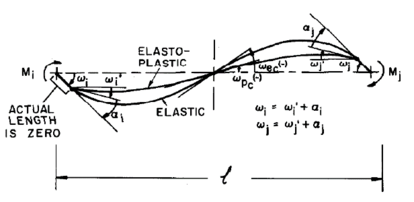
Two-component model [151]

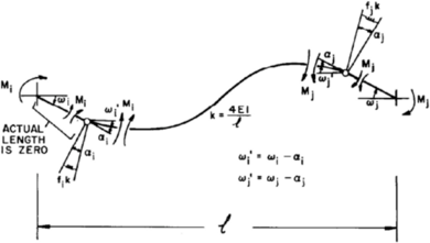
(a) One-component model [152]

Figure 87. Nonlinear two and one component models for a nonlinear beam element

A complete model for the analysis of seismic response of RC structures was proposed by Banon et al.1981 [157]. The one-component model in its original form describes the nonlinear behavior of the girder. The hysteretic moment-rotation relation is based on a modified Takeda model. In order to reproduce the "pinching" effect due to shear and bond deterioration, a nonlinear rotational spring is inserted at each member end. The hysteretic model of the nonlinear springs is based on a bilinear skeleton curve with strength decay under large deformations and includes the effect of "pinching" during reloading.

The method of defining backbones curves is well approved as the most practical way in performance based design, such backbones or capacity curves can be represented by moment-rotation or force-deformation relation for ductile and brittle behavior respectively [158] [16].

Figure 88 shows a general representation of lumped plasticity model with assigned capacity curves for plastic hinges. Backbone curve can be obtained from experimental results (Figure 88.b) as the envelope of the hysteretic behavior, they can be classified according to the level of the ductility into three levels [16] as shown in Figure 88.c. For cyclic loading a hysteretic response must be assigned to the plastic hinge, the hysteretic response must reflect the main characteristics of the cyclic behavior (e.g. strength reduction, stiffness degradation, buckling in compressed reinforcing bars, cracks opening and closing and bond-slip degradation).

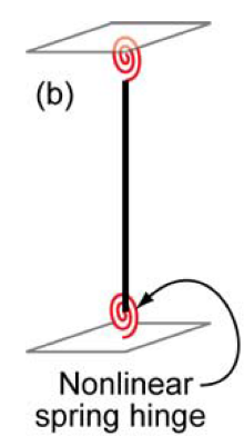
(a)) Lumped plasticity model
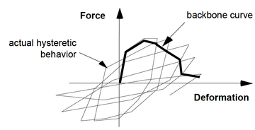
	(b) Backbone representation of hysteretic behavior [16]
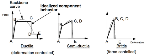
	(c) Backbone curve types [16]
Figure 88. Nonlinear behavior of lumped plasticity model

As mentioned before, Takeda model has been widely used for reinforced concrete simulation, however, many calibrated models have been developed recently. The most recent model is Ibarra et al.2005 [2]that is based on modifying three of the basic hysteretic models used in seismic demand evaluation to include deterioration properties: bilinear, peak-oriented, and pinching. The modified models include most of the sources of deterioration: i.e. various modes of cyclic deterioration and softening of the post-yielding stiffness, and also account for a residual strength after deterioration. The models incorporate an energy-based deterioration parameter that controls four cyclic deterioration modes: basic strength, post-capping strength, unloading stiffness, and accelerated reloading stiffness deterioration. Figure 89 shows the main hysteretic features of Ibarra model

Some types of concentrated hinge models employ axial load-moment (P-M) yield surfaces. Whereas these models generally do a good job at tracking the initiation of yielding under axial load and bending, they may not capture accurately the post-yield and degrading response. On the other hand, some hinge elements with detailed moment-rotation hysteresis models may not capture P-M interaction, except to the extent that the moment-rotation response is defined based on average values of axial load and shear that are assumed to be present in the hinge.

(a) Basic strength deterioration	(b) Post-capping strength deterioration
(c) Unloading stiffness deterioration	(d) Accelerated reloading stiffness deterioration
(e) Basic pinching model rules	(f) Modification in pinching according to reloading
Figure 89. Hysteretic bases of Ibarra et al. 2005 model [2]

2.2 Distributed plasticity models

From the physical behavior point of view, the damage in reinforced concrete structures is not lumped in a specific section, hence, spreading the plasticity along a specific length gives more accuracy to represent the nonlinear behavior of RC structure.

The first model which accounts for the spread of inelastic deformations into the member was introduced by Soleimani et al.1979 [159]. In this model a zone of inelastic deformations gradually spreads from the beam-column interface into the member as a function of loading history. The rest of the beam remains elastic. The fixed-end rotations at the beam-column interface are modeled through point hinges which are inserted at the ends of the member. These are related to the curvature at the corresponding end section through an "effective length" factor which remains constant during the entire response history. The model of Soleimani was further improved by Meyer et al. 1983 [160], by proposing different way to calculate the stiffness of the plastic zone during reloading and incorporating Takeda's law to describe the hysteretic behavior. This model was used to simulate the nonlinear behavior of beam and column with counting for the axial load. Further development of Meyer's model to incorporate the effect of shear and axial load has been done by Roufaiel and Meyer 1987 [161]. Another approaches were proposed by Filippou and Issa 1988 [162], in this model the element is divided into a finite number of short subelements. Each subelement describes a single effect, such as inelastic behavior due to bending, shear behavior at the interface or bond-slip behavior at the beam column joint.

Distributed plasticity models were stated at the beginning into displacement method (stiffness method). In this approach the unknowns are the displacement and cubic interpolation functions are used to approximate the deformation along the beam-column element. The first displacement-based model used the cubic Hermitian interpolation functions to describe the deformation of the element along its length. Relation between the element deformation and nodal displacement of the beam-column element represented in Figure 90 is writing as follow:

$\left\{\left.d(x)\right\}\right.=\left[N\right]\left\{\left.\delta \right\}\,\right.$

(76)

Where ${\textstyle d(x)}$ is the transverse and longitudinal displacement along the longitudinal axes (x), ${\textstyle \left[N\right]}$ is the matrix of the interpolation functions and ${\textstyle \left\{\left.\delta \right\}\,\right.}$ is the vector of the nodal displacements presented in Figure 90. Equation (76) can be written as :

$\left\{\left.{\begin{matrix}u(x)\\v(x)\end{matrix}}\right\}\right.=\left[{\begin{matrix}{N}_{1}&0&0\\0&{N}_{3}&{N}_{4}\end{matrix}}\,\,{\begin{matrix}{N}_{2}&0&0\\0&{N}_{5}&{N}_{6}\end{matrix}}\right]\,\left\{\left.{\begin{matrix}{\begin{matrix}{u}_{i}\\{\nu }_{i}\\{\theta }_{i}\end{matrix}}\\{u}_{j}\\{\begin{matrix}{\nu }_{j}\\{\theta }_{j}\end{matrix}}\end{matrix}}\right\}\right.$

(77)

where

${\begin{array}{ll}\displaystyle {N}_{1}=1-{\frac {x}{L}}&\displaystyle {N}_{4}={\frac {{x}^{3}}{{L}^{2}}}-2{\frac {{x}^{2}}{L}}+x\\\displaystyle {N}_{2}={\frac {x}{L}}&\displaystyle {N}_{5}=-2{\frac {{x}^{3}}{{L}^{3}}}+3{\frac {{x}^{2}}{{L}^{2}}}\\\displaystyle {N}_{3}=2{\frac {{x}^{3}}{{L}^{3}}}-3{\frac {{x}^{2}}{{L}^{2}}}+1&\displaystyle {N}_{6}={\frac {{x}^{3}}{{L}^{2}}}-{\frac {{x}^{2}}{L}}\end{array}}$

(78)

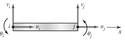
Figure 90. Nodal displacement of beam-column element in 2D [163]

The generalized deformations of the problem are the axial strain ε(x) and the curvature about the z-axis φ_z (x)_. Under the assumptions that displacements are small and plane sections remain plane the section deformations "generalized deformations" a(x) are related to the nodal displacements by:

$\left\{\left.a(x)\right\}\right.=\left\{\left.{\begin{matrix}\epsilon (x)\\\varphi z(x)\end{matrix}}\right\}\right.=$$\left\{\left.{\begin{matrix}{u}^{'}(x)\\{v}^{'}(x)\end{matrix}}\right\}\right.=$$\left[B\right]\left\{\left.\delta \right\}\,\right.$

(79)

Where ${\textstyle \left[B\right]=\,\left[dN\right]}$ , the derivative of the interpolation function matrix. Using the principal of virtual displacement of the principal of minimum potential energy, the element stiffness matrix can be writing as the integral of the section stiffness matrix ${\textstyle \left[k\right]}$ :

$\left[K\right]=\int _{0}^{L}{\left[B\right]}^{T}\left[k\right]\left[B\right]{d}_{x}$

(80)

The section stiffness matrix ${\textstyle \left[k\right]}$ relates the section forces with the corresponding deformations:

$\left\{\left.D(x)\right\}\right.=\left[k\right]\left\{\left.a(x)\right\}\right.$

(81)

Where ${\textstyle \left\{\left.D(x)\right\}\right.}$ is the vector of the section forces "the generalized stresses"; the axial force N(x) and the bending moment M_z(x) at section x.

The main shortcoming of this classical finite element displacement-based approach is their inability to describe the behavior of the member near its ultimate resistance and after the onset of strain softening, this is because of assumption of cubic interpolation functions, which result in a linear curvature distribution along the element. This assumption leads to satisfactory results under linear or nearly linear response. However, when the reinforced concrete member undergoes significant yielding at the ends, the curvature distribution becomes highly nonlinear in the inelastic region. This requires the use of a very fine discretization in the inelastic regions of stiffness based elements. This shortcoming has been demonstrated in the interesting study developed by Zeris and Mahin 1988 and 1991 [164], [165]; by studying the softening behavior of a cantilever beam it has been observed that assumed curvature distribution deviates significantly from the actual distribution during element softening, as the sharp jump in the curvature value near the fixed end. Results of this study are shown in Figure 91 as presented by [166]

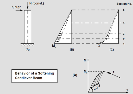
Figure 91. softening behavior for cantilever beam [166], (A) member and loading, (B) Moment distribution, (C) Curvature distribution, (D) Moment-Curvature relation.

It has been agreed that a more convenient format for distributed plasticity models is in terms of force method (flexibility method) where the unknowns are the forces, which implies assuming force interpolation functions. This approach uses the generalized deformation of the element instead of the displacement at the joints. The generalized deformation for the beam-column element represented in Figure 92 are: end rotations relative to the chord and the axial differential displacement, these deformations are demonstrated in

Figure 92.a. Accompaniment element forces "called as the generalized forces" are demonstrated in Figure92.b

(a) Generalized deformations	(b) Generalized forces
Figure 92. Beam-column element in force-based method

Assuming that the bending moment distribution inside the element is linear and that the axial force distribution is constant, the section forces "generalized stresses" can be related to the element force in a similar concept of equation (76) as follow:

$\left\{\left.D(x)\right\}\right.=\left[b\right]\left\{\left.Q\right\}\,\right.$

(82)

${\textstyle \left[b\right]}$ is the matrix containing the force interpolation functions, ${\textstyle \left\{\left.Q\right\}\,\right.}$ is the vector of the generalized force demonstrated in

Figure92.b. Equation (92) can be written as follow:

$\left\{\left.{\begin{matrix}N(x)\\{M}_{Z}(x)\end{matrix}}\right\}\right.=\left[{\begin{matrix}0&0&1\\{\frac {x}{L}}-1&{\frac {x}{L}}&0\end{matrix}}\right]\,\left\{\left.{\begin{matrix}{Q}_{1}\\{Q}_{2}\\{Q}_{3}\end{matrix}}\right\}\right.$

(83)

The application of the virtual force principle yields the element flexibility

$\left[F\right]=\int _{0}^{L}{\left[b\right]}^{T}\left[f\right]\left[b\right]{d}_{x}$

(84)

Where ${\textstyle \left[f\right]}$ is the section flexibility, equation (81) can be rewritten as:

$\left\{\left.a(x)\right\}\right.=\left[f\right]\left\{\left.D(x)\right\}\right.\,$

(85)

The advantage of this formulation is satisfying the element equilibrium in a strict sense. Whatever the material nonlinearity take place at the section level and even as the element starts softening when deformed beyond its ultimate resistance, the assumed internal force distributions are exact [166].

In1984 the concept of fiber element was introduced by kaba and Mahin [167]. In this model the element is discretized into longitudinal sections called control sections and each section is divided into several fibers. The constitutive relation of the section is not explicitly specified, but is derived by integrating the response of the fibers, which follow the uniaxial stress-strain relation of the particular material as shown in Figure 93.

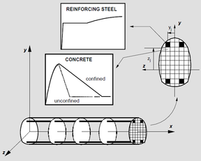
Figure 93. Fiber element model [166]

This concept has been well accepted and approved as a good approach to simulate the nonlinear behavior of reinforced concrete beams and columns. Two main models have been developed according to the concept of fiber element. Displacement-Based and Force-Based models termed in this research as DB and FB respectively. Both approaches allow plastic hinges to form at any location and account for axial moment interaction by integrating the force-deformation response at sections along the element length. The number of sections and their location is determined by the numerical quadrature rule, such as those based on Gauss quadrature are used to integrate the element force-deformation relationship.

DB follow the standard finite element approach, in which the element displacement field is expressed as a function of the nodal displacement using displacement interpolation functions. The displacement field is approximate; thus several displacement-based elements are required along the length of a frame member to represent the deformations in a plastic hinge region [168] [169]. In contrast, FB approach interpolates the section forces in terms of the basic forces, satisfying equilibrium even in the range of nonlinear material response [123] [170]. The primary advantage of FB formulation over the DB is the ability to use one force-based element to simulate the material nonlinear response of a frame member, compared with several displacement-based elements, thereby keeping the number of degrees of freedom in the structural model to a minimum.

While distributed plasticity formulations model variations of the stress and strain through the section and along the member in more detail, important local behaviors, such as strength degradation due to local buckling of steel reinforcing bars, or the nonlinear interaction of flexural and shear, or the degradation due to bond-slip degradation are difficult to capture without sophisticated and numerically intensive models. On the other hand, concentrated hinge/spring models, may be better suited to capturing the overall response, through calibration using member test data on phenomenological moment-rotations and hysteresis curves as described in the previous subsection.

3 Structural component-based vs continuum mechanics-based approaches

3.1 Introduction

This section presents a comparison between a models derived from structural component-based approaches and the more complex models that are based on continuum mechanics formulation. Models involved in this section are the simple ones based on concentrated and distributed plasticity approaches described in the previous section, and the continuum-based model developed in Part I of this dissertation. The monotonic and cyclic experiments described in section ‎6 of Part I are simulated with both models, obtained results are compared with the ones from the experiments.

3.2 Monotonic loading simulation

The one floor RC frame experiment [Pires 1990] described in subsection ‎6.2.1 is simulated with lumped and distributed plasticity models. The concentrated plasticity model is implemented in software package SAP-2000 v.16 [171] by using the displacement formulation [172], without accounting for shear-generated deformation. Second-order effects are taken into account. Zero-length flexural and axial-flexural hinges are assigned to beams and columns, respectively. As well, shear hinges are considered for both types of members. Hinges are located at faces of joints. In flexural and axial-flexural hinges, parameters of initial and further branches of the assigned backbones curves are obtained according [173] and [12], respectively. In shear hinges, parameters of initial branch are obtained according to [173], and after-yield behavior is assumed to be totally brittle. Neither shear-flexural interaction nor shear-axial-flexural interaction is considered. Figure 94 shows the capacity curves obtained by the aforementioned concentrated plasticity model with the experimental one. Results from Figure 94 shows that model is able to capture only the initial stiffness of the frame. The rest of the behavior is not captured by the model, degradation due to flexural cracking is not represented, nor the maximum capacity. As a first observation, the concentrated plasticity model with the parameters from [173] and [12] provides poor representation of the real behavior of this one floor RC frame.

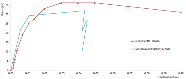
Figure 94. Capacity curves for [Pires 1990] RC frame. Experimental vs. concentrated plasticity model.

[Pires 1990] RC frame is also simulated by the distributed plasticity models. This involves the fiber element with both DB and FB approaches. The FEM package SeismoStruct V6.5 [112] is used to perform this analysis. In the DB models, each member is discretized with four 2-node finite elements. In the FB models, a single element with five integration points represents each member. For both FB and DB models, sections are discretized into 250 fibers. Second-order effects are accounted for. As in the concentrated plasticity model, the interaction between shear and flexure is not taken into consideration. Each fiber along the cross section is associated with a uniaxial stress-strain relation; concrete fibers are assigned to Mander et al. 1988 model [174] considering the confinement effect for the fibers in the inside the confinement zone, steel fibers are assigned to Menegotto and Pinto 1973 model [175] with isotropic hardening.

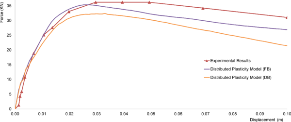
Figure 95. Capacity curves for [Pires 1990] RC frame. Experimental vs. distributed plasticity models.

Obtained results by the DB and FB models are plotted with the experimental one in Figure 95. Plots from Figure 95 show a good agreement between the numerical models and experimental behavior, initial stiffness and subsequent degradation due to flexural cracking are well represented till reaching the maximum capacity. After reaching the maximum capacity, both DB and FB models started a rapid strength reduction, while the real behavior showed some ductility. Comparing between FD and DB response, the FB approach showed better agreement in representing the maximum strength.

For comparison with the results obtained by the continuum-base model in subsection ‎6.2.1, Figure 96 displayed the plots obtained in Figure 50, Figure 94 and Figure 95. Plots from Figure 96 show the superiority of the continuum-based model to describe the response of the RC frame, results of the structural component-based model show that the concentrated plasticity model describes satisfactorily the initial slope, but fails to predict the cracking and, therefore, the onset of the overall yielding; force and displacement ductility are underestimated because of the conservative assumptions in the predefined plastic hinges. Distributed plasticity models perform better, particularly the one based on FB formulations.

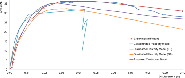
Figure 96. Capacity curves for [Pires 1990] RC frame. Experimental vs. structural and advanced models.

The two floor RC frame experiment [Vecchio and Emara 1990] described in subsection ‎6.2.2 is also simulated similarly to the previous experiment. Concentrated and distributed plasticity models are used to describe the behavior of the two floor RC frame.

Obtained capacity curve by the contracted plasticity model is displayed with the experimental behavior in Figure 97. Plots from Figure 97 drive similar observation to Figure 94. The concentrated model describes satisfactorily the initial slope, but fails to predict the cracking and, therefore, the onset of overall yielding. The maximum capacity in terms of force is underestimated because of the conservative assumptions in the predefined plastic hinges. The final failure is earlier because the actual ductility of members is also underestimated by the assumed moment-rotation laws

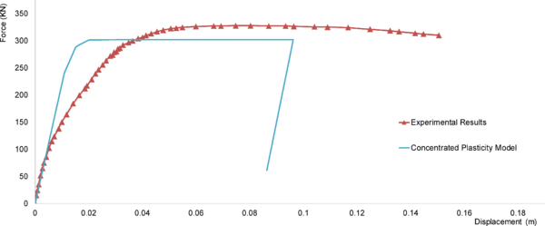
Figure 97. Capacity curves for [Vecchio and Emara 1990] RC frame. Experimental vs. concentrated plasticity model.

Similarly, to the previous experiments, the two floor RC frame is simulate as well using the fiber element with DB and FB approaches. Figure 98 shows the obtained capacity curves and experimental ones. In general, better agreement is obtained by the distributed plasticity models, particularly FB model captured the maximum strength and the ductility phase, however, earlier degradation is predicted by DB and FB models.

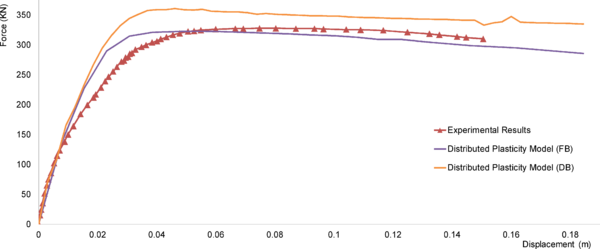
Figure 98. Capacity curves for [Vecchio and Emara 1990] RC frame. Experimental vs. distributed plasticity models.

For comparison with continuum-based model, Figure 104 collects the plots of Figure 58, Figure 97 and Figure 98. Plots from Figure 99 show again the superior ability of the proposed continuum-based model to reproduce the experimental results along the whole displacement range. Regarding the lumped plasticity model, accuracy can be considered satisfactory, given the important simplifications involved in that model. Regarding the distributed plasticity models, Figure 99 shows that they perform better, particularly FB. DB model exhibits less accuracy, because the mesh is too coarse. However, these models cannot capture adequately the gradual progression of the global softening after the initial overall yielding, due to lack of consideration of the concrete tensile strength. Noticeably, the negative slope of the final branches is due to second-order effects.

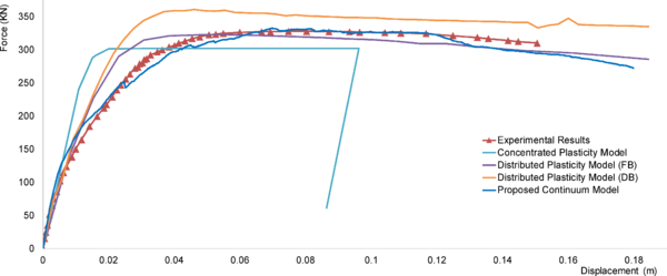
Figure 99. Experimental and simulated capacity curves for [Vecchio and Emara 1990] RC frame. structural and advanced models

An overall comparison between the experimental observation and the ones obtained by the structural and continuum-based models are demonstrated in Table 12.

Table 12. Experimental vs. numerical results [Vecchio and Emara 1990] frame. structural and advanced models

	SAP2000	SeismoStruct FB	SeismoStruct DB	ABAQUS	Experiment
Ultimate Force (KN)	302	322	361	333	332
First Plastic Hinge Developed at	Beam 1st Story	Beam 1st Story	Beam 1st Story	Beam 1st Story	Beam 1st Story
Failure Mechanism	6 Plastic Hinges	6 Plastic Hinges	6 Plastic Hinges	6 Plastic Hinges	6 Plastic Hinges
Joints Damage	N/A	N/A	N/A	YES	YES
Force at First Crack in Beam First Story	N/A	N/A	N/A	61	52.5
Force at First Crack in the column at the base	N/A	N/A	N/A	135	145
Force at first yielding in the column's reinforcement	N/A	295	327	305	323
N/A Not Available

3.3 Cyclic loading simulation

This subsection presents similarly compression to the previous subsection. The cyclic loading experiments described in subsection ‎6.3 of Part I are simulated with structural component-based models. Results are compared with the real behavior and the one previously captured by the proposed continuum mechanics-based model.

As an observation from the previous subsection, the fiber element models showed higher capacity in representing the real behavior. Hence, the concentrate plasticity models are excluded from the cyclic loading simulation and just fiber models are implemented. As well, the advanced FEM code OpenSEES [176] is used to implement the fiber model. The open source OpenSEES provides wide range or materials and elements models, as well different algorithms are available to perform nonlinear static and dynamic analysis with powerful convergence controlling.

Since the cyclic behavior of RC structures involves new degradation modes, additional elements are incorporated in the simulation. Standard fiber models nor the concentrated plastic models are able to capture the bond-slip degradation and the results represented in the so called pinching effect. To overcome this shortcoming, the strain penetration model developed by Zhao and S. Sritharan 2007 [124] is assigned into a zero length element at the elements edges where bond-slip effects are expected to occur. The strain penetration model [124] is the most common strategy to capture bond-slip effect in structural component-based models; it is assumed that bars are well anchored and slip is entirely due to strain penetration in the anchorage zone. Then, rotations at member ends are generated. A constitutive hysteretic stress-slip law for steel bars based on pull-out tests is generated; it is used for zero-length elements situated at column bottom and is integrated into a global fiber model. Figure 100.a shows the hysteretic stress-slip law for steel bars, while Figure 100.b displays the implementation of the zero length in fiber model. This model is implemented in OpenSEES [176].

(a) Influence of pinching parameter on bar stress vs slip	(b) Integrating fiber element with strain penetration model
Figure 100. Strain penetration model for bond-slip effect Zhao and S. Sritharan 2007 [124]

The RC column experiment Tanaka 1990 [98] described in subsection ‎6.3.1 is discretized with one 2-node finite elements using the force-based formulation, and one zero-length element to represent bond-slip. Sections are discretized in fibres using Concrete01 material for both confined and unconfined concrete. while Steel02 material is used for reinforcement. Figure. 101 shows the uniaxial cyclic behavior for both concrete and steel materials model OpenSEES code.

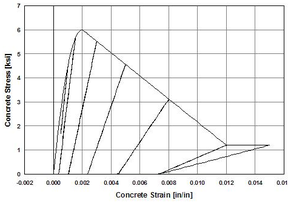
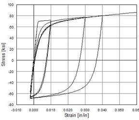
(a) Concrete01 model	(b) Steel02 model
Figure 101. Uniaxial cyclic model for concrete and steel OpenSEES

Concrete confinement is taken into consideration using the modified kent and park 1971 [177] model, this model has been developed by Scott et al. 1982 [178] by incorporating the confinement effects on the maximum strength and strain. Stress-strain response for confined and unconfined concrete according to Scott model is shown in Figure 104.a.

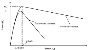
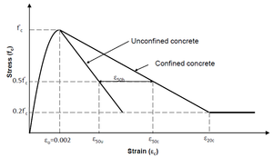
(c) Scott et al. 1982 concrete model [178]	(d) Kent and Park 1971 [177]
Figure 102. Confinement effect on Uniaxial concrete stress-strain relation

The following formulations are used to calculate Concrete01 model parameters (MPa)

${\rm {For\,}}{\epsilon }_{c}\,\leq \,0.002K\qquad f_{c}=Kf_{c}^{'}\left[{\frac {2{\epsilon }_{c}}{0.002K}}-\left({\frac {{\epsilon }_{c}}{0.002K}}\right)^{2}\right]$ ${\rm {For\,}}{\epsilon }_{c}>\,0.002K\qquad f_{c}=Kf_{c}^{'}\left[1-{z}_{m}\left({\epsilon }_{c}-0.002K\right)\right]\,\geq 0.{2Kf}_{c}^{'}$ ${z}_{m}={\frac {0.625}{{\epsilon }_{50h}+{\epsilon }_{50u\,}-0.002K}}\qquad \qquad K=1.25\left[1+{\frac {{\rho }^{''}{f}_{yh}}{{f}_{c}^{'}}}\right]$ ${\epsilon }_{50h}={\frac {3}{4}}{\rho }^{''}{\sqrt {\frac {{b}^{''}}{S}}}\qquad {\epsilon }_{50u}={\frac {3+0.29{f}_{c}^{'}}{145{f}_{c}^{'}-1000}}\qquad {\rho }^{''}={\frac {2\left({b}^{''}+{d}^{''}\right){{A}_{s}}^{''}}{{b}^{''}{d}^{''}S}}$

(86)

In equations (86), f^'_c and f_yh are concrete compressive strength and steel yield strength respectively of transverse bars, ρ´´ is volumetric ratio of confining hoops to volume of concrete core measured to the outside of the perimeter hoops, where b´´ and d´´ are the width and depth of the confined core respectively, A_s´´ is the cross-sectional area of the hoop bar and S is the center to center spacing of the hoops. ε_50u and ε_50c are the strain corresponds to 50% of concrete maximum compressive strength for unconfined and confined concrete respectively, while ε_50h is the differencebetween the previous two values as shown in Figure 104.b. Implementing concrete model Concrete01 requires the strain at the maximum strength to be calculated ε₀ as 2f^'_c/E_c where E_c is concrete modulus of elasticity, as well the ultimate compressive strain shall to be defined, in Figure 104.b this corresponds to ε_520c.In this work ε_cu is used to express the ultimate compressive strain, it’s calculated according to the formulation proposed by [178] as :

${\epsilon }_{cu}=0.004+0.9\,\left({\frac {{f}_{yh}{\rho }_{sh}}{300}}\right)$\qquad ${\rho }_{sh}={\frac {{A}_{sh}}{Sd}}$

(87)

ρ_sh and f_yh are the transverse reinforcement ratio and yield stress respectively A_sh is the total area of transverse bars acting in the considered direction of the section, d is the effective depth of the section.

Steel02 material model is based on the isotropic hardening model for steel developed by Menegotto and Pinto 1973 model [175]. Parameters of this model are obtained from OpenSEES software.

The zero-length element is discretized as any section along the length of the element, Steel02 material is replaced with the strain penetration material. This model follows the phenomenological hysteretic law proposed displayed in Figure 100.a; one of the parameters that governs reloading branch is the pinching factor R_c shown in Figure 100.a. This parameter modifies completely the response of the zero-length element; consequently, this will alter significantly column behavior. R_c = 1 represents perfect bond situation and, thus, no pinching effect; lower values of R_c correspond to significant pinching. For the simulation of Tanaka column, R_c = 0.6 has provided the best results.

Figure 103 displays comparisons between experimental and numerical hysteresis loops obtained with the abovementioned structural component-based model.

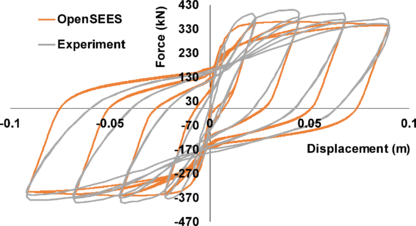
Figure 103. Hysteretic force displacement response of [Tanaka 1990] column. Experimental vs. structural component-based model

Plots from Figure 103 show that the structural component-based model is able to capture acceptably the envelope of column response, however, the maximum strength is not well captured nor the degradation upon unloading and reversing the loading direction as well the pinching effect. For comparison with results obtained previously in the Part I by the continuum-based model, Figure 104 collects the plots from Figure 67.b and Figure 103

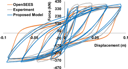
Figure 104. Hysteretic force displacement response of [Tanaka 1990] column. Experimental vs. structural and advanced model

Results from Figure 104 show that the simplified model reveals less accurate in comparison with the continuum-based model.

Similarly to the simulation of Tanaka column, the one floor RC frame described in subsection ‎6.3.2 of Part I is analyzed with the aforementioned structural component-based model. Herein the zero-length element is assigned in three places where bond-slip is expected to be significant: columns base, columns top, and beam ends.

As discussed previously, this model is particularly sensitive to pinching factor R_c; As a preliminary attempt, the calibrated value from the simulation of the bridge column R_c = 0.6 is used in the three locations. Analogously to Figure 103 comparison between experimental and numerical hysteresis loops obtained by the structural component-based is demonstrated in Figure 105.

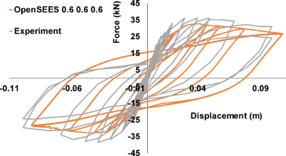
Figure 105. Hysteretic force displacement response of [Pires 1990] frame. Experimental vs. structural component-based model (constant Rc)

Plots from Figure 105 show that the response obtained by the structural component-based model is shifted from the experimental response, this can be explained by the high flexibility generated by the low values of R_c in the three locations.

To stabilize the numerical response, the value of R_c must be calibrated in each location individually. After several attempts, better results are obtained by assigning the values 0.8, 0.9 and 0.4 to the columns base, columns top, and beam ends respectively. Analogously to Figure 105, Figure 106 shows a comparison between the experimental response and the one obtained with the aforementioned R_c values.

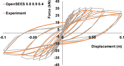
Figure 106. Hysteretic force displacement response of [Pires 1990] frame. Experimental vs. structural component-based model (varying Rc)

Plots from Figure 106 show that the structural component-based model shows very good agreement in terms of capturing the unloading stiffness and pinching effect, however the maximum strength is not well captured, as well as the strength reduction.

Analogously to Figure 104, Figure 107 displays comparisons between experimental and numerical hysteresis loops obtained with the proposed continuum-based and the simplified one with the abovementioned values of R_c. Figure 107 collects the plots from Figure 77.b and Figure 106. Results from Figure 107show that the structural component-based model has better capacity in representing the pinching effect, maximum capacity and strength reduction are better represented by the continuum-based model.

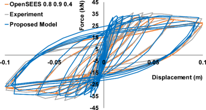
Figure 107. Hysteretic force displacement response of [Pires 1990] frame. Experimental vs. structural component-based (varying Rc) and advanced model

4 Developed model for non-ductile RC structures simulation

After verifying the capacity of structural component-based models to represent the nonlinear behavior of RC structures, this section presents an advanced structural component-based model for seismic simulation of non-ductile RC structures. The developed model accounts for flexure, shear and axial deterioration modes. It involves, advanced lumped plasticity models, as well FB fiber element model and Limit state models for shear and axial failure in columns. The developed model is numerically efficient, thus being suitable for day use in earthquake engineering.

4.1 General description

Based on experiments and observations from past earthquakes, FEMA-P695 [18] has identifies the main element (local) deterioration modes and global collapse mechanisms of RC frames. Deterioration modes of beam-column elements are classified into three categories: flexure hinging, compressive failure and shear failure. Collapse mechanisms are classified in vertical and sidesway. Collapse mechanisms and deterioration modes are closely related: flexure hinging leads usually to sidesway collapse, and column shear deterioration subsequently can lead to loss in vertical carrying capacity and vertical collapse. Modeling this phenomenon is a complex task due to the interaction among moment, shear and axial forces. Furthermore, the interaction among these modes influence the entire structure and determine its global collapse mechanism. This issue is particularly important in RC building frames when they are designed without any seismic provision, and highly vulnerable to severe earthquakes. This type of structures is commonly known as “non-ductile RC frames”. In them, the influence of brittle deterioration modes (e.g. shear and axial) of columns is high because the common requirements that ensure ductility (strong column-weak beam, and confinement of critical regions, among others) are not fulfilled.

Unfortunately, non-ductile RC frames are extremely common in seismic regions, due to, among other reasons, underestimation of actual seismicity, loose requirements of past design codes, lack of fulfillment of current codes, and poor construction practices. On the other hand, seismic design and analysis of actual buildings require dealing with complex models, having many degrees of freedom. Moreover, most of analyses are nonlinear; dynamic nonlinear analyses are becoming more frequent. Even Incremental Dynamic Analysis (IDA) starts being more popular. IDA Vamvatsikos, Cornell 2002 [17] consists in determining the dynamic structural response to one or more seismic inputs (accelerograms) scaled with increasing factors; obviously, this is highly time-consuming. Frequently, these models are excessively simplified, accounting only for flexure deterioration modes, and can lead to misleading results. Consequently, there is a strong need for models that combine numerical efficiency and accuracy, mainly with the consideration of all deterioration modes and their interaction.

In this section, a structural component-based model is developed to simulate the nonlinear dynamic behavior of non-ductile RC structures. This model is used in the next section to perform a numerical study on the relation among the non-simulated deterioration modes of the elements of non-ductile RC frames and their final capacity. The developed model is implemented in OpenSEES code McKenna et al. 2000 [176] accounting for flexure, shear and axial deterioration modes.

4.2 Implantation in finite element analysis

4.2.1 RC frame model

As described in the previous subsection, non-ductile RC structures might face non-common local deterioration modes. These modes are basically represented in shear degradation in columns, subsequently generate loss in the axial carrying capacity and ending by vertical collapse. The interaction between flexure, shear and axial forces in the nonlinear domain makes the simulation of such deterioration modes not easy. However, the consequences of disregarding deterioration modes other than flexure hinging have been studied by several researchers. The previous studies used post processing approach to check if any non-simulated deterioration mode has occurred, then the collapse capacity of the structure is modified by probabilistic formulations [179]. Aslani and Miranda [180], developed fragility functions based on 92 cyclic tests of RC columns; those functions detect column shear and axial failure by post-processing the results from ordinary dynamic analysis. Columns yielded first in flexure and then failed in shear, this being the so-called “flexure-shear” deterioration mode. Aslani and Miranda define four damage states: (1) light cracking, (2) severe cracking, (3) shear deterioration and (4) loss of load- carrying capacity; the proposed fragility functions predict the probability of each damage state in terms of drift ratio, axial load ratio and transverse reinforcement amount. Research by Aslani and Miranda show that the proposed fragility functions provide improved estimates of the probability of experiencing these damage states. This formulation was recommended by [179] [181] [182]. Liel [181] carried out IDA analyses for a 8-story RC frame using the fragility functions developed by Aslani and Miranda. Results show that, for some records, collapse is governed by shear and axial deterioration modes; for some non-ductile structures, collapse probability increases by 30% after taking into account those modes. Other displacement-based models have been proposed to capture this complex response: [183] [184] [1] [185]. Elwood model [1], succeeds in capturing the aforementioned failure modes and has been verified and recommended by several researchers and standards [186] [187] [18]. This model uses zero-length shear and axial springs that are series connected with the column.

Starting from the previous studies, a model for the nonlinear static and dynamic simulation of non-ductile RC frames accounting for flexure hinging in beams and four deterioration modes in columns is developed herein. Deterioration modes in columns are: (i) flexure hinging, (ii) flexure-shear, (iii) flexure-shear-axial, and (iv) compressive. After flexure hinging, flexure-shear consists in shear failure of concrete, yielding or fracture in the transverse reinforcement, while there is still some axial carrying capacity. After this, flexure-shear-axial represents the loss of this capacity. Compressive failure of columns is characterized by concrete crushing, longitudinal reinforcement buckling, and transverse reinforcement yielding or fracture. Flexure hinging and compressive failure are described with distributed plasticity (fiber models) using FB formulation described in subsection ‎2.2 of this part. Flexure-shear and flexure-shear-axial are simulated with shear and axial springs, respectively. Pure shear failure (force exceeds resistance) is not considered inside the analysis, given that is usually preceded by the other failures; this verification is carried out during post-processing. Bond-slip effect at the top and bottom of columns is considered by attaching linear rotational spring, in beams this effect is considered implicitly in the hysteretic behavior of the lumped plastic hinges at the beams edges. Frame elements are discretized as depicted in Figure. 108.

(a) Overall view of a frame discretization	(b) Detail of a column element joint (sketch A)
(c) Detail of a beam-column joint (sketch C)	(d) Detail of bottom column slip spring (Sketch B)
Figure 108. Discretization of beams and columns

Figure. 108.a displays an example of the discretization of a frame, additional nodes are used to account for the higher stiffness of beam-column joints; mass nodes are located at intersection points and spring nodes are situated at the ends of the joints and at intermediate sections inside beams. Figure. 108.b provides a closer view of a column element. Figure. 108.c shows a closer view of a beam-column joint, in beams, flexure hinging is modelled with zero-length rotational springs (concentrated plasticity); at the top of columns, three springs are connected in series, two nonlinear shear and axial springs represent flexure-shear and flexure-shear-axial failures, respectively, and linear represent bond-slip degradation. Nonlinear behavior of axial and shear spring is described in the following subsection ‎4.2.4, while the rotational stiffness of the slip spring is described in subsection ‎4.2.2. Figure. 108.d shows a closer view of the bottom nodes of columns where a linear rotational spring is attached for bond-slip effect, similar to the spring at the top of the column. In general, the nonlinear behavior of beams is described with concentrated plasticity models while columns are analyzed with distributed plasticity fiber models; therefore, the main segments of beams exhibit linear behavior, and those of columns behave nonlinearly.

This model is implemented in OpenSEES code [176]; the drift capacity model developed by Elwood 2004 [1] is used to describe flexure-shear and flexure-shear-axial deterioration of columns, representing by the axial and shear springs at the top of columns (Figure. 108.c). Second order effects are accounted for by a P-delta analysis.

The consideration of the plasticity and cyclic behavior in beams and columns is described next.

Beams. As described before, concentrated plastic model is used to describe the nonlinear behavior of beams element by attaching nonlinear rotational springs at the beam edges. The behavior of the rotational springs is based on the modified hysteretic model developed by Ibarra et al. 2005 [2]. Three of the basic hysteretic models used in seismic demand evaluation are modified in this model to include deterioration properties: bilinear, peak-oriented, and pinching. The modified models include most of the sources of deterioration: i.e. various modes of cyclic deterioration and softening of the post-yielding stiffness, and also account for a residual strength after deterioration. The models incorporate an energy-based deterioration parameter that controls four cyclic deterioration modes: basic strength, post-capping strength, unloading stiffness, and accelerated reloading stiffness deterioration. Figure 109 shows the backbone curve of this model as well as the main parameters.

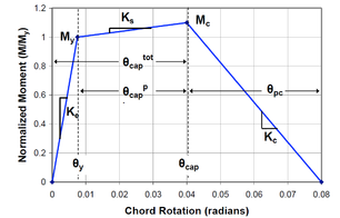
Figure 109. Backbone curve of Ibarra et al 2005 model [2].

Ibarra model can be considered as the most recent hysteretic model for seismic RC structures simulation, however, it involves many parameters to be defined. To understand better the physical behavior of each parameter among the possible prediction, Figure 110 provides information about the physical behavior contributing of each parameter, as well the possible approaches to determine these parameters.

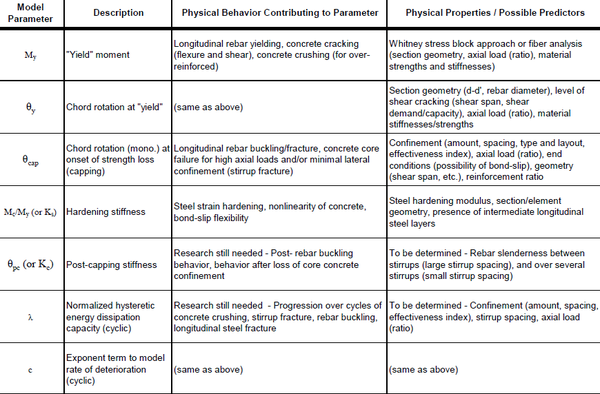
Figure 110. Description of Ibarra et al 2005 model parameters [188] .

As described in Figure 110, particular inputs of [2] model are obtained from the sectional analysis of the beams, and other parameters, such as the plastic rotations θ_cap,pl, θ_pc and the energy dissipation parameter λ , are obtained from the formulations proposed by Haselton et al 2008 [188].

${\theta }_{cap,pl}=0.12\,{\left\{{\frac {max\left(0.01,{\frac {{\rho }^{'}{f}_{y}}{{f}_{c}^{'}}}\right)}{max\left(0.01,{\frac {\rho {f}_{y}}{{f}_{c}^{'}}}\right)}}\right\}}^{0.225}\left(1+\right.$$\left.0.55{a}_{sl}\right){\left(0.16\right)}^{\nu }{\left(0.02+40{\rho }_{sh}\right)}^{0.43}\,(continued)$ ${\textstyle {\left(0.54\right)}^{0.01{{f}_{c}^{'}c}_{units\,}}{\left(0.66\right)}^{0.1{S}_{n}}\,{\left(2.27\right)}^{10\rho }}$ ${\theta }_{pc}=\left(0.76\right){\left(0.31\right)}^{\nu }{\left(0.02+40{\rho }_{sh}\right)}^{1.02}\,\leq 0.1$ $\lambda =\left(170.7\right){\left(0.27\right)}^{\nu }{\left(0.1\right)}^{\frac {S}{d}}\,$

(88)

In the previous formulations; ${\textstyle \nu }$ is the ratio of the axial forces on the gross section capacity calculated as P/A_gf' _c, ρ_, ρ^' and ρ_sh are the reinforcement ratios of positive, negative and transverse steel respectively, S/d the ratio of transverse reinforcement spacing to the depth of the section. a_sl indicator variable (0 or 1) to signify possibility of longitudinal rebar slip and taks value of slip is possible, f^'_c and f_y are the concrete and steel yield strength respectively, c_units is a unit conversion variable that takes a value of 1 when f^'_c and f_y are in MPA and 6.9 for Ksi. S_n is the rebar bucking coefficient and can be calculated as (S/D_b)(f_y/100)^0.5 for f_y in MPA, where D_b is the longitudinal bar diameter.

Columns. Distributed plasticity model is used to describe the nonlinear behavior of column element. The fiber model described in subsection ‎2.2 is implemented using the force-based formulation. Integration (along the column length) is carried out by Gauss–Lobatto quadrature rule with five integration points. Concrete and steel uniaxial behavior are considered similarly to the simulation of cyclic loading described in subsection ‎3.3. Using “Concrete01” model, with zero tensile strength and a parabolic segment in compression followed by a linear descending branch. Concrete confinement is also taken into consideration as [178]. Behavior of reinforcement bars is simulated with “Steel 02” model. Refer to subsection ‎3.3 of this part for more information about implementing material models.

4.2.2 Bond-slip effect in columns

Longitudinal reinforcement slip at column ends is represented by an increase in the corresponding rotation angles. As discussed previously, this effect is simulated by zero-length linear rotational springs, Figure. 108.c.d Stiffness of springs is selected as recommended by [189]:

${C}_{slip}={\frac {8\,{f}_{b}}{{D}_{b}\,{f}_{s}\,}}\,E{I}_{flex}$

(89)

In equation (89), D_b is the bar nominal diameter, EI_flex is the column effective flexure rigidity at first yield, f_s is the stress in the steel bars, can be taken equal to yield stress f_y Berry et al. 2004 [190], and f_b is the bond stress ${\textstyle 0.8\,{\sqrt {{f'}_{c}}}}$ (MPa) [187].

4.2.3 Effective lateral stiffness of columns

The objective of this subsection is to obtain the effective lateral stiffness of columns (in terms of EI_eff) accounting for flexure, slip and shear flexibility. The yield drift displacement Δ_y can be estimated as the sum of displacements due to these effects:

${\Delta }_{y}\,={\Delta }_{flex}+{\Delta }_{slip}+{\Delta }_{shear}$

(90)

Displacements in right hand side of equation (90) can be estimated [191] as:

${\Delta }_{slip}\,={\frac {L\,{D}_{b}\,{f}_{s}\,{f}_{y}}{8\,{f}_{b}}}$ ${\Delta }_{shear}\,={\frac {2\,{M}_{SP}}{{GA}_{eff}}}$	(91)
${\Delta }_{flex}\,={\frac {{L}^{2}}{6}}\,{f}_{y}={\frac {{L}^{2}}{6}}\,{\frac {{M}_{SP}}{{EI}_{flex}}}$

In equation (91), L is column length, ϕ_y is yield curvature, M_SP is moment at spalling of concrete, and EI_flex and GA_eff are the effective flexure and shear stiffness, respectively. Flexure displacement Δ_flex is obtained assuming that column is clamped at both ends and that curvature varies linearly along height. M_SP corresponds to concrete strain 0.004. EI_flex can be determined from the moment and curvature at first yield as shown in Figure 111. First yield is defined to be the point first occurs of either bar yielding in tension or when maximum compressive strain in concrete reaches 0.002.

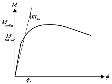
Figure 111. Flexural effective stiffness and moment curvature relationship

Finally, the response of column before yielding can be approximated as linear-elastic with single effective stiffness EI_eff is expressed as:

${EI}_{eff}={\frac {{L}^{2}}{6}}\,{\frac {{M}_{SP}}{{\Delta }_{y}}}$

(92)

This stiffness is used in the idealized bilinear model for the shear displacement law in the next section. Since this model assumes that flexure failure will occur before shear one, equation (92) can be considered as a good approximated statement to add the influence of the different components of displacement at the flexural yielding state.

4.2.4 Column flexure-shear and flexure-shear-axial deterioration models

Several studies [192] [193] [194] have shown that shear strength decays with increased inelastic deformation; hence, flexure-shear deterioration model should be based on force and deformation. Also, after flexure-shear degradation, columns tend to lose their vertical carrying capacity [195]. In this work, flexure-shear and flexure-shear-axial deterioration are described with shear and axial limit curves [1] referring to shear and axial springs that are series connected with the fiber elements, Figure. 108.c.

Shear spring predicts deterioration according to an empirical drift function [196] based on experimental results; later, axial deterioration arises from sliding along an inclined shear crack. Next equations provide drift limit angle at flexure-shear and flexure-shear-axial deterioration (Δ_s / L and Δ_a / L, respectively):

${\frac {{\Delta }_{s}}{L}}={\frac {3}{100}}+4\,{\rho }_{sh}-{\frac {1}{40}}\,{\frac {\nu \,}{\sqrt {{{f}^{'}}_{c}}}}-$${\frac {1}{40}}{\frac {P}{{A}_{g}{{f}^{'}}_{c}}}\geq {\frac {1}{100}}$	(93)
${\frac {{\Delta }_{a}}{L}}={\frac {4}{100}}\,{\frac {1+\mathrm {{tan}^{2}} \,\theta }{\mathrm {tan} \,\theta +P\,{\frac {S}{{A}_{sh}{\,f}_{sh\,}{d}_{c}\mathrm {tan} \,\theta }}}}\quad \quad$

In equations (93), ρ_sh is the transverse reinforcement ratio, ν is the demanding shear stress (V / A_g), P / A_g f_c ' is the demanding axial load ratio, d_c is the column core depth (between centre lines of stirrups), S is the transverse reinforcement spacing, A_sh and f_yh are area and yield point of transverse reinforcement, and θ is the critical crack angle (θ = 65º, [196]). Units are in MPa.

When the response reaches the shear limit curve (Δ_s / L in equation (93)), the backbone curve of the shear spring is shifted to a descending branch [1], total response of the shear spring is the sum of shear failure and flexural yielding in the column as shown in Figure 112. The total lateral stiffness K^t_deg shown in Figure 112 is obtained by combining the negative stiffness of the descending branch K_de with the stiffness given by equation (92). The total lateral stiffness K^t_deg can be calculated by assuming that axial failure occurs when shear capacity degrades to almost zero, K^t_deg can be calculated by the following equation:

${K}_{deg}^{t}=\,{\frac {{V}_{u}}{{\Delta }_{a}-{\Delta }_{s}}}$

(94)

V_u is the ultimate shear capacity of the column, and it's calculated according to ASCE41-13 [158] using the following formulation in MPa units:

${V}_{u}=\,k{V}_{0}=k\left[{\frac {{A}_{sh}{f}_{yh}d}{s}}+\lambda \left({\frac {0.5{\sqrt {{f}_{c}^{'}}}}{\frac {M}{Vd}}}{\sqrt {1+{\frac {{N}_{u}}{0.5{\sqrt {{f}_{c}^{'}{A}_{g}}}}}}}\right)0.8{A}_{g}\right]$

(95)

In the previous formulation, the ratio M/V is taken as the half column height, and N_u as the initial gravity force, k is a factor that takes a value according to the ductility displacement and it's assumed to be equal to 1, Δ_s is the calculated displacement at shear failure and Δ_a is the calculated displacement at axial failure that corresponds to the axial load measured at shear failure. Other symbols in equation (95) are described previously.

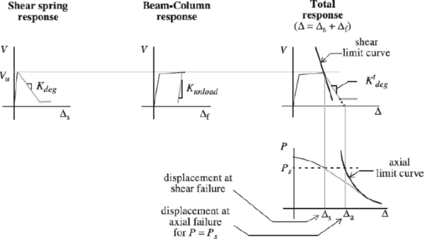
Figure 112. Determination of the degradation stiffness Kdeg [1]

Since the beam column element and the shear spring are in series, the shear degradation stiffness can be calculated from the following equation.

${K}_{deg}=\,{\left({\frac {1}{{K}_{deg}^{t}}}-{\frac {1}{{K}_{unload}}}\right)}^{-1}$

(96)

Where K_unload is the unloading flexural stiffness of the column, and for the bilinear idealization of moment-curvature relationships of beam column element, it's taken for fixed column equal to 12EI_eff/L³. Where EI_eff is determined in equation (92). The effective stiffness of column subjected to lateral load is also reported in FEMA-356 [12] as shown in Table 13. Effective flexural stiffness of reinforced concrete column, [10].

Table 13. Effective flexural stiffness of reinforced concrete column, [12]

Component	Flexural Rigidity
Columns with compression due to design gravity loads > 0.5 Agf’c	0.7 EcIg
Columns with compression due to design gravity loads < 0.3 Agf’c or with tension	0.5 EcIg

Where I_g is the moment of inertia for the gross section.

5 Nonlinear dynamic analysis of non-ductile RC structures

5.1 Introduction

To highlight the importance of hidden failure modes (flexure-shear deterioration of columns followed by loss of bearing capacity), a numerical study on the relation among the non-simulated deterioration modes of the elements in non-ductile RC frames and their final capacity is presented in this section. This study reports on the so-called “Structural Resurrection” phenomenon in Incremental Dynamic Analysis. It consists in some structures collapsing under a certain accelerogram, although resisting the same accelerogram scaled by a bigger factor.

The developed model in the previous section is implemented in OpenSEES code [176] and used to study the nonlinear static and dynamic behavior of two non-ductile structures. The first structure is a three floor prototype building described in subsection ‎5.2, while the second structure the seven floor Van Nuys Hotel building described in subsection ‎5.3. The model is verified with experimental results from a shaking table test in order to check its reliability.

To point out the importance of non-simulated failure modes, the developed model is adapted in the numerical study into four models that differ in the number of deterioration modes that are taken into consideration; from least to most:

• First model. Corresponds to simple models that are commonly used in earthquake engineering. Material degradation is simulated through concentrated/distributed plasticity (beams/columns). Second-order effects are accounted for. Bond slip in columns is accounted for through the simplified formulation in equation (89). This model is able to simulate only sidesway collapse.

• Second model. Like first model although without second-order analysis.

• Third model. This model is similar to first one, but considers also flexure-shear deterioration by attaching a shear spring in series with a bond slip element at each column top (Figure. 108.c).

• Fourth (developed) model. This model is generated following third one by incorporating also axial springs (Figure. 108.c). For the sake of better numerical stability, these springs are incorporated only to columns that have experienced flexure-shear deterioration. This model is able to predict sidesway and vertical collapse.

Previous models are used in the next subsections to perform different static and dynamic analysis.

5.2 Three floors prototype building

5.2.1 Prototype description

The first studied non-ductile structure is a prototype 3 RC story framed building that had been intentionally designed only for gravity loads [197] [198]. This building has been also studied by other researchers [199] [200]. Figure 113 displays a plan view (Figure 113.a) and an elevation (Figure 113.b) of the prototype building; floor plan is rectangular (12.19 m × 23.16 m) and story height is 3.66 m.

(a) Plan view	(b) Vertical view
Figure 113. Structural plan and section of the prototype building Bracci et al. 1992 [197]

The structure consists of 30.5 cm × 30.5 cm columns, 23 cm × 46 cm beams and 15.24 cm deep two-way solid slabs. Concrete strength is f_c’ = 24 MPa and steel yield point is 275 MPa. Geometry and reinforcement details for beams and columns are demonstrated Figure 114. Deeper description of the structure applied loads can be found in [197]. Noticeably, column section and transverse reinforcement amount are small.

A one-third scale model of a part of the prototype building was tested in a shaking table [197]. The results of the one third scale test are used to verify the reliability of the numerical model before performing the IDA study on the full scale prototype model. Next subsection presents the numerical simulation of the one third scale model, as well comparison with the experimental observations.

(a) Longitudinal beam reinforcement arrangement
(b) Longitudinal beam reinforcement sections
(c) Reinforcement arrangement for columns
Figure 114. Geometry and reinforcement details of the prototype building Bracci et al. 1992 [197]

5.2.2 Experimental verification

As described in the previous subsection, a one third scale model of the three floor prototype building has been tested on a shaking table by [197]. This subsection describes the numerical simulation of this test using the developed model (Model 4). Obtained results from the numerical models are verified with experimental ones. The aim of this verification is to validate the developed model to capture the experimental behavior of this one third scale model. These proofs consist in uniaxial shaking table testing of a one-third scale model representing a 3D frame of an internal bay in the short direction of the prototype building. A plan and vertical views of the one third scale model is shown in Figure 115. Materials properties from the experiments are described in Table 14 and Table 15.

Table 14. Concrete materials properties for the prototype one third scale test Bracci et al. 1992 [197]

Element	f'c (MPa)
Beams	35
Columns 1st floor	23.5
Columns 2nd floor	30
Columns 3rd floor	23.25

Table 15. Reinforcement steel properties of the prototype one third scale test Bracci et al. 1992 [197]

Bar No.	Db (mm)	fy (MPa)	fu (MPa)	Es (GPa)	Esh (MPa)
D4	5.7	468	503	214	5.17
D5	6.4	262	372	214	6.55
#11ga	3	386	482	205	5.1

Based on materials properties and reinforcement details for column and beams of the considered longitudinal frame shown in Figure 116, the relevant modeling parameters have been calculated following the formulations of the developed model in the previous subsection ‎4 and summarized in Table 16 and Table 17 for columns and beams respectively.

Table 16. Modeling parameters for columns of the prototype one third scale test

Location	Δs/L	Δa/L	Kdeg	Cslip (Kn.m)
1st floor-Interior	0.0296	0.0457	801	915
1st floor-Exterior	0.0314	0.0555	104	604
2nd floor-Interior	0.032	0.0562	101	1395
2nd floor-Exterior	0.0333	0.0647	56	921
3rd floor-Interior	0.0334	0.0727	38	1191
3rd floor-Exterior	0.034	0.08	29	786

Table 17. Modeling parameters for beams of the prototype one third scale test

Location	EIeff	My+ (Kn.m)	Mc+/ My+	θpl+	θpc+	My- (Kn.m)	Mc-/ My-	θpl-	θpc-	λ
Sec A	0.45 EI	38	1.05	0.0212	0.0552	23.73	1.05	0.0193	0.0552	56
Sec D	0.45 EI	38	1.05	0.0194	0.0552	44.7	1.05	0.0165	0.0552	56

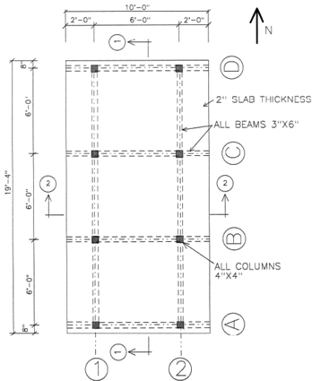
(a) Plan view

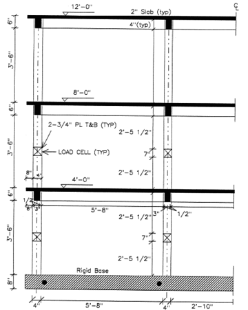
(b) Section 1-1

Figure 115. Structural plan and section of the prototype one third scale test Bracci et al. 1992 [197]

(c) Longitudinal beam reinforcement arrangement
(d) Longitudinal beam reinforcement sections
(e) Reinforcement arrangement for columns
Figure 116. Geometry and reinforcement details of the one third scale prototype test Bracci et al. 1992 [197]

The input motion of Taft earthquake and N21E component was selected for the shaking table motion. The original accelerogram shown Figure 117, has a total excitation time history of 54.4 sec with PGA equal to 0.156g at 9.1 sec. Original signal was scaled to adapt with the one third scale model by reducing the total time with a scale factor 1 / (3)^½, as well the maximum acceleration was scaled to 0.2g.

In the numerical simulation, damping is represented by a mass-proportional 2% Rayleigh model. Time step is 0.01 s.

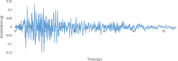
Figure 117. Accelerogram signal for original Kern County Earthquake of 21 Jul 1952 (Taft Lincoln School station-N21

During the analysis, neither flexure-shear nor flexure-shear-axial failure are detected in the analysis and damage is basically flexural in beams and columns; this result matches the observed damage [197]. Figure 118 displays a comparison between numerical and experimental time histories of the top floor relative displacement.

Figure 118. Top floor displacement of the prototype one third scale test. Modified Taft ground motion. Experiment vs. numerical model (Model 4).

Plots from Figure 118 shows a satisfactory agreement between experimental and simulated results. Noticeably, higher discrepancies correspond to the last time interval (25-30 s), where important damage in the frame has been cumulated along the analysis.

This fit confirms accuracy and reliability of the developed model and the correct estimation of the parameters of the tested structure. After this verification, next subsection presents an Incremental Dynamic Analysis of the Prototype Building with real scale.

5.2.3 Incremental Dynamic Analysis

The prototype building described in subsection ‎5.2.1 is analyzed in this subsection. A 2D inner frame in the short direction (Figure 113) is studied. The effective flexure stiffness is estimated as 0.4 EI_g for beams. The obtained fundamental period in the analyzed direction is 1.148 s. Incremental Dynamic Analysis (IDA) is carried out for the same input considered in the shaking table test described in the previous subsection, using the original signal.

To study the dynamic behavior of the 2D frame, Model 1 (simplified) and Model 4 (developed) are considered. In Model 1, stiffness and mass-proportional Rayleigh damping is used; damping ratio is 5% at first and second modes. In Model 4, just mass-proportional damping (5%) is used; stiffness-proportional damping cannot be used due to unrealistically large damping forces resulted from sudden shear and axial deterioration of zero-length springs [191]. Concrete strengths for beams and columns are summarized in Table 18, while the calculated modeling parameters are summarized in Table 19 and Table 20.

Tabla 18. Concrete materials properties for the prototype building

Element	f'c (MPa)
Beams	24
Columns	24

Tabla 19. Modeling parameters for columns for the prototype building

Location	Δs/L	Δa/L	Kdeg	Cslip (Kn.m)
1st floor-Interior	0.026	0.0264	213	17097
1st floor-Exterior	0.029	0.0373	590	14088
2nd floor-Interior	0.0274	0.03	270	15159
2nd floor-Exterior	0.03	0.0479	372	12993
3rd floor-Interior	0.03	0.0479	372	12993
3rd floor-Exterior	0.0314	0.0656	88	11626

Tabla 20. Modeling parameters for beams of the prototype building

Location	EIeff	My+ (Kn.m)	Mc+/ My+	θpl+	θpc+	My- (Kn.m)	Mc-/ My-	θpl-	θpc-	λ
Sec A	0.23EI	523	1.05	0.025	0.06	376	1.05	0.029	0.06	61
Sec D	0..23EI	523	1.05	0.029	0.06	725	1.05	0.029	0.06	61

Using Model 1 and Model 4, IDA study has been conducted on the frame shown in Figure 113. Obtained IDA curves by both models are displayed in Figure 119. IDA curves are presented in terms of maximum interstory drift ratio vs. spectral acceleration for the building fundamental period (S_a(T₁)). Comparison between curves for models 1 and 4 shows that the simplified model showed the capacity to resist higher acceleration, while the advanced model predicted the collapse before. Final state "collapse mode" for both models are displayed in Figure 120, it can be seen that each model showed different collapse mechanism. Model 1 (Figure 120.a) predicts sidesway collapse due to flexure hinging of first floor columns at S_a = 0.5 g (Figure 119), while Model 4 (Figure 120.b) detects an earlier flexure-shear deterioration of first floor columns followed by flexure-shear-axial failure (loss of axial carrying capacity) of the inner first floor columns at S_a = 0.425 g (Figure 119). As a preliminary observation from Figure 119; Flexural-shear degradation subsequent by loss of axial load carrying capacity might occur in this frame before reaching the final collapse due to flexural hinging. The simplified model "Model 1" represents the common used models in earthquake engineering, is not able to capture such degradation, this leads to overestimating in the seismic capacity of the considered frame.

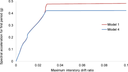
Figure 119. IDA curves of the prototype building. Taft ground motion. Models 1 and 4

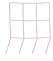
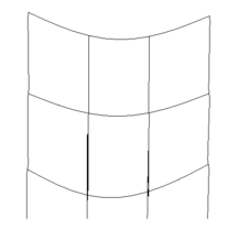
(a) Model 1	(b) Model 4
Figure 120. Collapse modes of the prototype building. Taft ground motion. Models 1 and 4

Figure. 121 displays plots of axial force vs. story drift for the first floor columns; displayed plots correspond to the final time-history analysis using Model 4 (S_a = 0.425 g, Figure 119). Figure. 121 confirms that columns C2 and C3 reach their axial limit curves. The collapse mechanism can be seen when column C2 reaches its limit curve and starts to loss part of the axial load carrying capacity following the axial limit curve as shown in Figure. 121.b, the loss of the axial force was compensated by column C3 and increase in the axial load can be seen in Figure. 121.c, this additional axial load ended by reaching C3 its axial limit curve, at this moment more axial force has been transferred to C1 and instability is detected by large vertical displacement "vertical collapse". Since [1] model assumes that flexure-shear and flexure-shear-axial deterioration precedes shear strength failure, it is necessary to verify that the demanding shear force does not exceed the corresponding capacity [158]. This is verified by comparing the shear response history with the shear strength at each increment following the formulation of ASCE 41-13 in Equation (95). Figure. 122 displays the shear response history bounded by the shear capacity history. Plots from Figure. 122 show that the demanding shear forces do not exceed the strength. Noticeably, the highest variability of shear strength in columns C2 (Figure. 122.b) is due to the bigger oscillation of demanding axial force, as being outer columns. As well, the observed peaks correspond to limitations of moment/shear ratio [158].

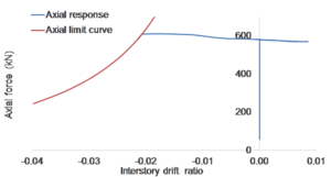
(a) Column C1 (left column in Figure 113)	(b) Column C2 (second column in Figure 113)
(c) Column C3 (third column in Figure 113)	(d) Column C4 (right column in Figure 113)
Figure 121. Axial force of first floor columns vs. drift for the prototype building. Taft ground motion. Model 4

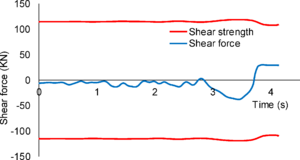
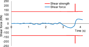
(a) Column C1 (left column in Figure 127)	(b) Column C2 (second column in Figure 127)
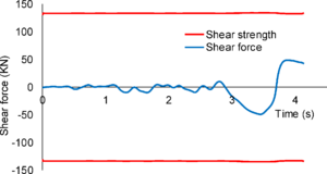
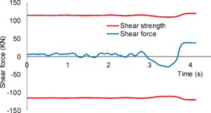
(c) Column C3 (third column in Figure 127)	(d) Column C4 (right column in Figure 127)
Figure 122. Prototype model. Shear force history of 1st floor columns. Taft ground motion scaled to Sa = 0.425 g. Model 4

5.3 Seven floors Van-Nuys hotel building

5.3.1 Building description

The seven floor Van Nuys Hotel is analyzed similarly to the prototype building in the previous subsection. This structure is considered by the Pacific Earthquake Engineering Research Center (PEER) as a test-bed structure. This construction has been studied by several researchers [201] [202] [203] [204] [205] [206] and had been instrumented prior the 1994 Northridge earthquake.

This building [207] has a non-ductile 7-story RC framed structure without basements, and its plan configuration is rectangular (19.20 m × 45.72 m), being uniform along the building height. There are 3 bays in one direction and 8 bays in the other direction (Figure 123). The long direction is oriented east-west. The building is almost 20 m tall: the first story is 4.15 m high and stories 2 through 7 are 2.59 m high. The building is located in San Fernando Valley, California, being built in 1966 and having experienced several significant earthquakes. Suffered minor structural damage and extensive non-structural damage during 1971 San Fernando earthquake, and extensive structural damage during 1994 Northridge earthquake.

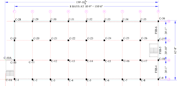
Figure 123. Structural plan of Van Nuys Hotel [206]

The RC structure has two-way flat slabs with beams in the perimeter; inner columns have square cross-section and façade columns have rectangular section. Design was carried out using 1963 version of ACI-318; columns do not have ductile detailing. Strength of columns concrete is f _c’ = 34.5/27.5/21 MPa for the 1^st/2^nd/higher stories. Strength of beams and slabs concrete is f _c’ = 27.5 MPa at 1^st and 2^nd floors and f _c’ = 21 MPa at floors 3 to 7. Columns reinforcement is made of A432-62T (Grade 60) steel; beams and slabs reinforcement is ASTM A15-62T and A305-56T (Grade 40). The geometry and reinforcement of columns and beams are displayed respectively in Figure 124 and Figure 125. Deeper description of the structure and the loads can be found in [206].

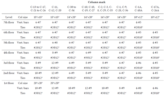
(a) Reinforcement table

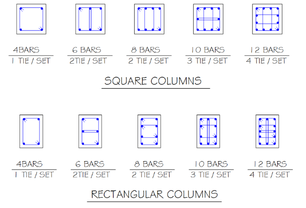
(b) Reinforcement arrangement

Figure 124. Columns reinforcement Van Nuys Hotel [206]

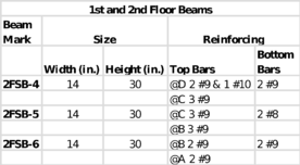
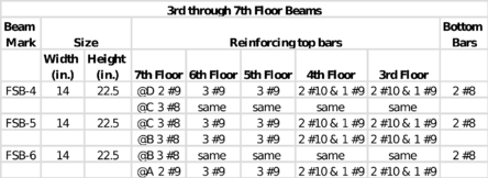
Figure 125. Beams reinforcement tables Van Nuys Hotel [206]

5.3.2 Building modelling

Previous 2D Incremental Dynamic Analyses studies have been carried out in the short direction of Van Nuys Hotel. Vamvatsikos et al. 2003 [207] studied the dynamic response of this structure by performing IDA calculations under twenty seismic records. Flexure and flexure-shear deterioration of columns were represented by non-interacting translation and rotational springs, respectively. The input severity is quantified by the spectral response ordinate for the first mode S_a(T₁,0.05), and the magnitude of the response is quantified by the maximum interstory drift (along building height and input duration). Figure 126 displays an IDA curve for 1979 Imperial Valley record, Plaster City station. The first mode period is taken as 0.8 s; the spectral ordinate for the unscaled record is S_a(0.8,0.05) = 0.194 g. In this study, structural resurrection phenomena has been detected as shown in Figure 126. The physical meaning of this phenomena can be explained as a given structure collapses under a certain input but is able to resist the same accelerogram scaled with a bigger factor. In IDA studies, the structural resurrection is defined as an extreme hardening with negative slope, the structure exhibits collapse "high value of drift or displacement" before recovering.

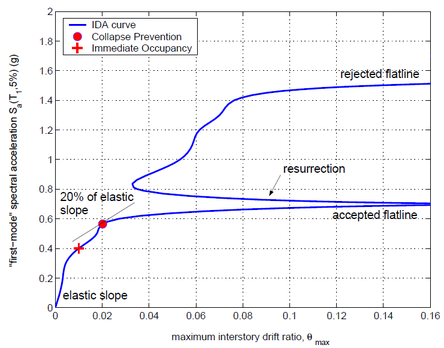
Figure 126. IDA curves for Van Nuys hotel frame with structural resurrection.Imperial Valley ground motion, Plaster City station Vamvatsikos et al. 2003 [207]

Another study was conducted by Krawinkler 2005 [206]; flexure-shear failure was accounted for using a force-distortion law. This model is independent on load history and drift demand. The initial shear strength is selected according to [208] assuming that concrete contributes only to the minimum residual capacity; and the post-peak response is modelled as highly brittle.

The structural resurrection circumstance is highly surprising, although conceivable, given the big uncertainties inherent in nonlinear time-history analyses. To investigate completely the feasibility of structural resurrection, it is necessary to account for all the degradation and failure modes and their interaction.

In this work, the developed model in subsection ‎4 is used to study the seismic performance of Van Nuys Hotel in the short direction. The structure is represented by a 2D facade frame (Figure 127), corresponding to axis 9 in Figure 123. The observed structural resurrection in previous study conducted by [207] is also investigated.

To estimate the contribution of this frame to the initial lateral stiffness of the building, a linear 3D model of the whole structure is built using SAP 2000 [Computers & Structures 2015]. The obtained percentage is 18%; mass is assigned accordingly. The seismic weight corresponds to D + 0.3 L (D: dead load, L: live load). Additional loads are applied at column ends to better represent the actual observed 3D behavior. The effective flexure stiffness of the beams is estimated as 0.35 EI_g in the first, sixth and seventh floors and 0.4 EI_g for the other floors; these coefficients are selected according to the sectional parameters. Concrete strengths for element in each floor are displayed in Table 21, the relevant modelling parameters for columns and beam are summarized respectively in Table 22 and Table 23.

Tabla 21. Concrete materials properties for the Van Nuys Hotel building

Element	f'c (MPa)
Beams 1ST and 2nd floor	27.5
Beams 3rd to 7th floor	20
Columns 1st floor	34.5
Columns 2nd	27.6
Columns 3rd to 7th	21

Table 22. Modeling parameters for columns the Van Nuys Hotel building

Location	Δs/L	Δa/L	Kdeg	Cslip (Kn.m)
1st floor-Interior	0.0282	0.0503	4620	131130
1st floor-Exterior	0.0278	0.0515	2060	131130
2nd floor-Interior	0.021	0.0455	1900	129240
2nd floor-Exterior	0.021	0.0355	2725	103103
3rd floor-Interior	0.0195	0.051	1210	94463
3rd floor-Exterior	0.0197	0.04	1422	75306
4t floor-Interior	0.02147	0.0563	945	94463
4t floor- Exterior	0.0212	0.0458	978	75306
5th floor though 7th floor	0.0226	0.0536	665	94463

Table 23. Modeling parameters for beams of the Van Nuys Hotel building

Location	EIeff	My+ (Kn.m)	Mc+/ My+	θpl+	θpc+	My- (Kn.m)	Mc-/ My-	θpl-	θpc-	λ
1st floor-B4-Ext	0.35 EI	230	1.05	0.0358	0.05	230	1.05	0.0358	0.05	106
1st floor-B4-Int	0.35 EI	230	1.05	0.0392	0.05	340	1.05	0.0333	0.05	106
1st floor-B5	0.35 EI	185	1.05	0.0392	0.05	340	1.05	0.03	0.05	106
1st floor-B6-Int	0.35 EI	230	1.05	0.0392	0.05	340	1.05	0.0333	0.05	106
1st floor-B6-Ext	0.35 EI	230	1.05	0.0358	0.05	230	1.05	0.0358	0.05	106
2nd floor-B4-Ext	0.4 EI	160	1.05	0.04	0.063	160	1.05	0.04	0.063	88
2nd floor-B4-Int	0.4 EI	160	1.05	0.0439	0.063	230	1.05	0.037	0.063	88
2nd floor-B5	0.4 EI	130	1.05	0.0437	0.063	230	1.05	0.034	0.063	88
2nd floor-B6-Int	0.4 EI	160	1.05	0.0439	0.063	230	1.05	0.037	0.063	88
2ndfloor-B6-Ext	0.4 EI	160	1.05	0.04	0.063	160	1.05	0.04	0.063	88
3rd-4th floors	0.4 EI	127	1.05	0.0473	0.063	275	1.05	0.034	0.063	88
5th floor	0.4 EI	127	1.05	0.0456	0.063	235	1.05	0.0354	0.063	88
6th floor	0.35 EI	127	1.05	0.0456	0.063	235	1.05	0.0354	0.063	88
7th floor-B4-Ext	0.35 EI	127	1.05	0.0417	0.063	160	1.05	0.0378	0.063	88
7th floor-B4-Int	0.35 EI	127	1.05	0.0432	0.063	190	1.05	0.0368	0.063	88
7th floor-B5	0.35 EI	127	1.05	0.0432	0.063	190	1.05	0.0368	0.063	88
7th floor-B6-Int	0.35 EI	127	1.05	0.0432	0.063	190	1.05	0.0368	0.063	88
7th floor-B6-Ext	0.35 EI	127	1.05	0.0417	0.063	160	1.05	0.0378	0.063	88

Figure 127. Model of the frame of the Van Nuys Hotel building

5.3.3 Push-over analysis

To point out the importance of non-simulated failure models in non-ductile RC structure, a nonlinear static analyses (pushover) are carried out using the simplified models (Model 1, Model 2 and Model 3) and the developed model (Model 4) described in subsection ‎5.1. This nonlinear static analysis furnishes for the next IDA analysis.

The pushing forces vary along building height as the first mode shape. Figure 128 and Figure 129 display, for each model, the capacity curves and the final states, respectively.

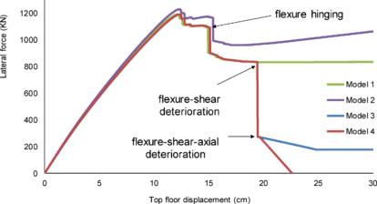
Figure 128. Capacity curve of the Van Nuys frame for the four models

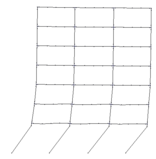
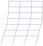
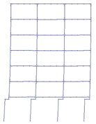
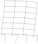
(a) Model 1	(b) Model 2	(c) Model 3	(d) Model 4
Figure 129. Deformation of Van Nuys frame at collapse. Four models

Figure 128 shows that, before reaching the maximum force capacity, the four models predict almost the same behavior; difference between Model 2 and the other models can be explained by influence of second-order effects. After this peak, all models describe flexure hinging degradation, followed by a near horizontal branch with highly similar results for models 1, 3 and 4. When flexure-shear deterioration is detected by third and fourth models, a brittle vertically descending branch is generated. Then, after reaching the residual strength, axial deterioration is detected by the fourth model; a linear descending branch (negative slope) follows that point. As expected, Figure 128 shows that, the more deterioration modes are accounted for, the less capacity is predicted; in other words, using over-simplified models leads to significant unconservative errors. Figure 129.a and Figure 129.b represent the sidesway collapse mechanisms detected by models 1 and 2, respectively; Model 2 predicts that hinging is distributed among several stories, but Model 1 indicated that it concentrates on first floor. Figure 129.c demonstrates that flexure-shear deterioration arose in first floor columns, thus generating a brittle collapse mechanism. In Figure 129.d, relevant flexure-shear-axial deterioration can be observed in right column (C36, Figure 123).

Figure 130 displays, from Model 3 and Model 4, plots of shear force vs. interstory drift ratio for first floor columns; Figure 130.a, Figure 130.b, Figure 130.c and Figure 130.d correspond to columns C9, C18, C27 and C36, respectively (Figure 123). Figure 130 shows that, after reaching the limit curve (Δ_s / L in equation (93)), shear response degrades until reaching a certain residual strength.

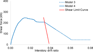
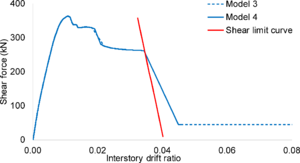
(a) Column C9 (left column in Figure 128)	(b) Column C18 (second column in Figure 128)
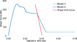
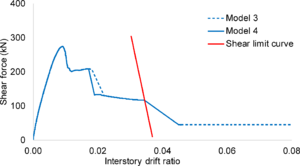
(c) Column C27 (third column in Figure 128)	(d) Column C36 (right column in Figure 128)
Figure 130. Van Nuys frame. First floor columns shear force vs. story drift. Models 3 and 4

Figure 131 displays plots of axial force vs. story interstory drift ratio for the most loaded column (C36). Figure 131 shows that, as highlighted by Figure 129.d, the limit axial curve is reached after flexure-shear deterioration.

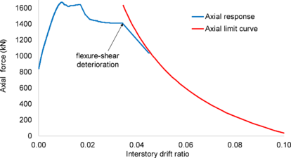
Figure 131. Van Nuys frame. Axial force vs. drift. First floor column C36. Model 4

5.3.4 Incremental Dynamic Analysis

Incremental Dynamic Analysis (IDA) is carried out for 1979 Imperial Valley ground motion, Plaster City station record, original signal is displayed in Figure 132. Noticeably, this input was also considered for the IDA analysis described in Figure 126 as described previously. The first mode period is taken as 1.3 s; the spectral ordinate for the unscaled record is S_a(1.3,0.05) = 0.244 g. Model 1 (simplified) and Model 4 (developed) are considered in this IDA study. In Model 1, stiffness and mass-proportional Rayleigh damping is used; damping ratio is 5% at first and second modes. In Model 4, just mass-proportional damping (5%) is used; stiffness-proportional damping cannot be used due to unrealistically large damping forces resulted from sudden shear and axial deterioration of zero-length springs [191]. In the most critical analyses, time step is 0.00002 s.

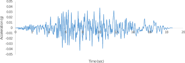
Figure 132. Accelerogram signal for original Imperial Valley ground motion, Plaster City station record

Figure 133.a displays IDA curves in terms of maximum interstory drift ratio vs. spectral acceleration at the building fundamental period (S_a(T₁)). Comparison between curves for Model 1 and Model 4 shows similarity with the results obtained in the IDA study for the prototype building in Figure 119. Results from Figure 133.a show that Model 1 predicts several segments with negative slope before reaching collapse at S_a = 0.68 g. Conversely, Model 4 provides a smoother behavior, with collapse at S_a = 0.49 g; it arises by loss of axial carrying capacity (flexure-shear-axial deterioration) of first floor columns C9, C18 and C27. Figure 134 presents four consecutive states of this brittle progressive collapse. State 1 (Figure 134.a) corresponds to flexure-shear deterioration of left column (C9). States 2 and 3 (Figure 134.b) include also flexure-shear deterioration of the other columns (C18, C27 and C36). In state 4 (Figure 134.d), columns C9, C18 and C27 also lose their bearing capacity. IDA curve from Model 1 predicts several structural resurrections in the range between S_a = 0.5 g and S_a = 0.68 g.

Figure 133.b displays IDA curves in terms of the top floor displacement, results from Figure 133.b show that the Model 1 predicts high capacity than the more sophisticated Model 4. Figure 133.b provides basically the same conclusions than Figure 133.a, although the maximum drift yields information of the behavior along the building height. Results from Figure 133 show that the judgment on reaching the collapse state is not clear by using the top floor displacement as a collapse reference, maximum top floor displacement for Model 1 at intensity S_a = 0.68 g is only 55 cm returns 2.7% top drift. Same intensity observed 14% of understory drift. Obviously this is a collapse state in the floor where this drift is detected.

Results from Figure 133 highlights again that the use of oversimplified models grossly overestimates the seismic capacity of non-ductile reinforced concrete structures. Although the structural resurrection is ignored in the construction of the fragility curves and first collapse is considered usually [17]. results obtained from Figure 133 and Figure 119 showed that the real collapse might occur before the considered one. Using models such Model 1 that are not capable to capture all the degradation modes has a direct effect on the fragility curve of the structure [181]. Results obtained by Liel [181] show that, collapse probability for non-ductile RC structures increases by 30% after taking into account the non-simulated failure mods.

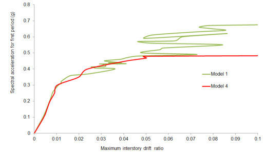
(a) IDA, interstory drift

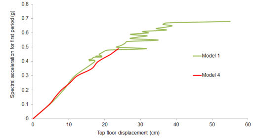
(b) IDA, top floor dispalcement

Figure 133. Van Nuys frame. IDA curves. Imperial Valley ground motion

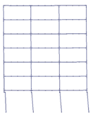
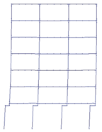
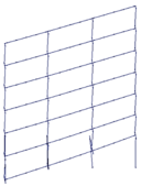
(a) State 1	(b) State 2	(c) State 3	(d) State 4
Figure 134. Van Nuys frame. Deterioration states. Imperial Valley ground motion. Model 4

Among the nonlinear dynamic analyses performed in this IDA study, Figure 135 displays meaningful top floor time-histories using Models 1 and 4 for some relevant intensities.

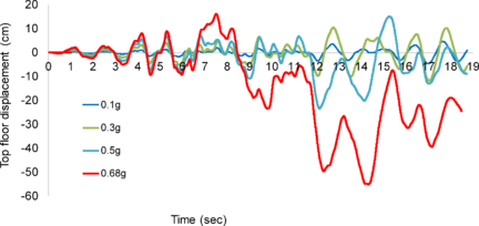
	(a) Model 1
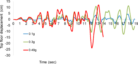
	(b) Model 4
Figure 135. Top floor time histories of Van Nuys frame with scaled (Sa(T1)) Imperial Valley ground motion

Plots from Figure 135.a show that the response for S_a(T₁) = 0.68 g is markedly nonlinear, since after 9 s the average displacement is clearly nonzero; this fits the observations from Figure 133.a. Analogously, Figure 135.b shows that, for Model 4, the response for S_a(T₁) = 0.49 g corresponds to collapse; this also fits Figure 133.b.

Figure 136 displays, similarly to Figure 131, plots of axial force vs. story drift for first floor columns; displayed plots correspond to the final time-history analysis using Model 4 (S_a = 0.49 g). Figure 136 confirms that columns C9, C18 and C27 reach their axial limit curves; bigger losses are experienced by columns C9 (mainly) and C18. Comparison among plots in Figure 136 shows that when a column reaches its axial limit curve, the subsequent axial force reduction is immediately followed by an increase in the other columns.

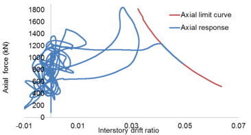
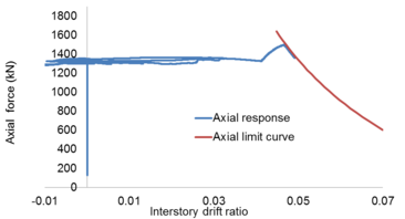
(a) Column C9 (left column in Figure 128)	(b) Column C18 (second column in Figure 128)
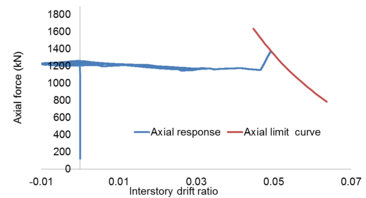
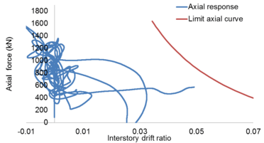
(c) Column C27 (third column in Figure 128)	(d) Column C36 (right column in Figure 128)
Figure 136. Van Nuys frame. Axial response of first floor columns vs. drift. Imperial Valley input. Model 4

As in the analysis of prototype building (Figure. 122), the shear force of first floor columns is compared with their shear capacity as shown in Figure 137 ; it is concluded that shear forces do not exceed the corresponding strength.

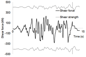
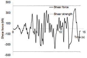
(e) Column C9 (left column in Figure 127)	(f) Column C18 (second column in Figure 127)
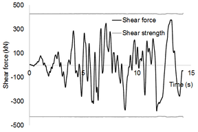
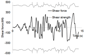
(g) Column C27 (third column in Figure 127)	(h) Column C36 (right column in Figure 127)
Figure 137. Van Nuys frame. Shear force history of 1st floor columns. Imp. Valley scaled to Sa = 0.49 g. Model 4

From the cases depicted in Figure 137, Figure 138 displays a zoom view of time histories of columns C9 and C36 in the latest time interval. Plots from Figure 137 show that, prior flexure-shear deterioration of column C9, both histories are similar; that failure generates a relevant reduction in shear force of column C9 and an equivalent increase in column C36. Flexure-shear-axial deterioration of column C9 arises (t = 14.10 s) after having reached the residual shear strength.

Figure 138. Van Nuys frame. Shear force time histories of columns C9 and C36. Imperial Valley scaled to Sa = 0.49 g. Model 4

6 Structural component-based approaches concluding remarks

The conclusion of this section are presented based on the order of conducted work as follow:

Structural component-based Vs. Continuum mechanics-based models:

In this part, structural component-based and common used models in earthquake engineering have been used to simulate the monotonic and cyclic behavior of tested reinforced concrete structures. Obtained results have been compared with experimental and numerical ones from the proposed continuum-based model presented in Part I.

The lumped plasticity models with predefined capacity curves (the parameters are obtained from seismic assessment standards) have been used to simulate the monotonic behavior of two reinforced concrete frames. Obtained results showed that such models are able to capture very well the initial stiffness of structures. Flexural craking, maximum capacity and the ductility phase are not well predicted. As a conclusion; the lumped plasticity models with predefined capacity curves showed inability to represent adequately the actual behavior of reinforced concrete frames.

Distributed plasticity models with fiber elements showed in general better performance in comparison with lumped plasticity approaches. Models with displacement and force based formulations have been used to simulate the monotonic behavior of the same two reinforced concrete frames. Obtained results have shown that the models exhibit earlier strength reduction in comparison with the actual behavior, maximum capacity is better represented by the FB models. The second order effects control the strength reduction and leads to underestimating in the maximum capacity.

Distributed plasticity models have been used as well to simulate the cyclic behavior of a bridge column and a reinforced concrete frame, a zero length element is added in the locations where bond-slip is expected to occur. The key parameter in the zero length element is the pinching effect parameter that affects the cyclic behavior of the assigned steel material in the zero length element. This parameter needs to be calibrated case by case and no general value can be assigned in all the location. However, after calibrating the pinching parameters a good agreement between the numerical and experimental behavior is achieved.

Obtained results from the previous simulations have been compared with the advanced model in Part I. Obtained results showed the superior ability of the proposed continuum-based model to reproduce the experimental results along the whole loading range. The pinching effect is better represented by the simple zero length element, however, the maximum strength and strength reduction is better represented by the continuum-based model.

Nonlinear dynamic simulation of non-ductile RC structures:

A computationally-efficient model for dynamic behavior simulation of 2-D RC frames under severe seismic excitation has been developed. The developed model used an advanced lumped plasticity model to represent the plasticity in beams, while the behavior of the columns is represented more accurately based on distributed plasticity. In the columns, the reinforcement bond-slip, flexure hinging, flexure-shear, flexure-shear-axial and compressive deterioration modes are taken into consideration. The capacity of the developed model has been verified in an existing non-ductile building and in a prototype building that have been intentionally designed without any seismic consideration. The developed model has been validated with tests of a reduced-scale laboratory model of the prototype building.

The obtained results show that the developed model, despite its moderate computational cost, detects and reproduces accurately the deterioration modes that are blind to the simplified models that are commonly employed in earthquake engineering. As well, the model is able to simulate accurately an experiment on a reduced scale model of the aforementioned prototype building. Comparison with the results from more simplified models highlights the importance of the hidden failure modes in the behavior of each element and in the overall collapse mechanisms. The use of oversimplified models can lead to important mistakes on the unsafe side, since the structural capacity is utterly overestimated. particularly, structural resurrection might be merely due to the use of too simple models.

Conclusions

In this final chapter the main contributions of this study are presented in terms

of achievements and in terms of concluding remarks. Future improvements and

future lines of work based on the expertise gained and on the main difficulties

found while developing this research are suggested at the end.

Achievements

The main aim of this study was to develop an advanced computationally efficient model for nonlinear seismic analysis of reinforced concrete structures. In this context, two advanced models have been developed respectively in Part I and Part II of this dissertation. Capacity of the developed models to capture the main characteristics of RC frames nonlinear cyclic behavior has been verified with experimental results, also with the results obtained from oversimplified models commonly used in earthquake engineering.

In Part I, the first model has been developed derived from continuum mechanics based-formulation. The model has been used to perform 3D FEM modeling of RC structures. In this context, concrete elements have been simulated using solid finite elements, while steel bars have been modeled by truss elements. Bond between steel bars and the surrounding concrete was considered to be perfect for the monotonic loading analysis. To reach the goal of cyclic loading simulation, an interface element has been used to simulate the bond-slip effects.

The first contribution was a new methodology for calculating the damage evolution "damage variables" in Concrete Plastic Damage Models "CPDM". Particular incorporation of this methodology in the CPDM originally developed by Lubliner et al 1989 [30] and further improved by Lee and Fenves [22] is provided. The second contribution in this study was a new modeling scheme to implement the interface bond-slip model of Murcia-Delso [20] [129] [133] in 3D simulation where two or more bars are crossing in the same region. The third contribution was to develop a technique to integrate the CPDM model with the interface bond-slip element to capture the crack opening and closing upon unloading and reversal loading. Combining the methodology for calculating damage evolution in CPDM, the modeling scheme of bond-slip model and the technique to integrate CPDM and bond-slip model resulted in an integrated continuum mechanics-based model. This model has been implemented in ABAQUS software [89]. The capacity of the model has been verified in terms of mesh insensitivity, capturing damage evolution of plain concrete, representing the entire range of deformation and damage of two RC frames and one RC bridge columns subjected to monotonic and cyclic loadings. Obtained results from the numerical model have been compared with experimental observations; proposed model showed a high capacity to capture adequately the cyclic and monotonic behavior of the tested structures, main characteristics of damage, strength reduction and stiffness degradation have been captured by the proposed continuum-based model. The development continuum mechanics-based model can be considered as an effective tool for small and mid-size simulation of reinforced concrete structures. Local behavior of concrete, steel among the bond between both materials under strong monotonic and cyclic loading can be studied and simulated accurately using the developed model. Although this model showed a satisfactory agreement with experimental results and succeeded to capture the entire range of loading, its computational cost is high.

In Part I, the developed model in Part I has been verified with oversimplified models derived from structural component-based approaches. The outcome of this study was the inability of these oversimplified models to capture adequately the nonlinear behavior of RC frames. However, some simplified models showed acceptable performance when special care is dedicated to the materials and elements models.

Since the model proposed in Part I is computationally expensive, Part II presented an advanced structural component-based model, this model is computationally cheap in comparison with the model in Part I and can acceptably capture the overall response of large size structures. This model has been used to perform nonlinear dynamic analysis of 2D non-ductile RC frames. The aim of developing this model was to study the relation between the hidden failure modes in non-ductile structures (e.g. flexural failure in columns subsequent with shear failure, shear failure in column subsequent by loss of axial load carrying capacity) and the overall collapse mechanism of the structures. The new contribution is developing the model by combining different pieces and generating a day use model, this model can be used to simulate the nonlinear dynamic behavior of large scale non-ductile structures considering different degradation modes in beams and columns. The model has been implemented in OpenSEES [176] finite element software using different pieces of pre-developed models to capture the nonlinear behavior of columns and beams. The model has been verified with experimental results obtained from shaking table test. After verifying the reliability of the model, it has been used to perform IDA study on two non-ductile structures. Obtained results showed the high capacity of the model to represent the dynamic behavior of non-ductile RC frames. Main achievement of developing this model was the ability to study the significant effect of shear-axial failure in columns on changing the collapse mechanism of the entire structure from sidesway to vertical in non-ductile frames. Simulating and tracking the collapse process was also a good benefit of the developed model. Developed model can be considered as a good tool for large scale dynamic simulation, particularly for non-ductile RC frames.

Conclusions

Obtained conclusions from this research are addressed as follow:

• Proposed methodology for calculating the damage variables "damage evolution" for concrete plastic damage models can be considered as a practical and efficient method to obtain these variables. The proposed methodology is mesh-insensitiveness and can reproduces adequately the damage evolution in concrete. Implementing this methodology in the Concrete Plastic Damage Model CPDM (Lubliner et al. 1989 [30], Lee and Fenves 1998 [22]) is relatively easy.

• Reinforcing bars can be simulated by simple truss elements with one degree of freedom in the longitudinal direction. Relation between truss elements and the surrounding solid elements "for concrete" can be simplified to a perfect bond conditions for monotonic loading. The embedded technique can be used to represent the bond between the reinforcing bars and concrete, this holds true for structures subjected only to monotonic loading with no reversal.

• The proposed modeling scheme for implementing the interface bond-slip elements (Murcia-Delso 2013 [20] [129] [133]) in 3D models is an efficient method. In comparision with the method proposed by (Murcia-Delso 2013 [20] [129] [133]), the proposed method simplifies the modeling and helps to overcome mesh difficulties and convergence problems. It's significantly effective in the case where two or more reinforcing bars are crossing in the same region (e.g. beam column joints, column slab joints).

• Proposed technique to integrate the CPDM and the bond-slip model by reducing the value of the compression recovery factor showed better results in comparison with the method proposed by (Murcia-Delso 2013 [20] [129] [133]) in terms of the dissipated energy. Using this technique for models with perfect bond conditions "no bond-slip elements" under cyclic loading shows that these models can capture the overall response but fails to capture the stiffness degradation as well as the pinching effect. While the method proposed by (Murcia-Delso 2013 [20] [129] [133]) by introducing discrete crack at the bottom of the columns, showed that even the model with perfect bond conditions can face some stiffness degradation due to the high flexibility introduced by the discrete crack.

• For continuum mechanics-based simulation, the proposed model in Part I involving the methodology for calculating the damage variables, the modeling scheme of bond-slip, the technique to integrate CPDM and bond-slip model is an integrated model that can be used to simulate the monotonic and cyclic behavior of RC frames till high stage of deformation.

• Oversimplified models that are based on lumped plasticity cannot capture the earlier degradation in the structure due to flexural cracking. These models underestimate the maximum capacity of the structure, particularly when they are assigned to beams and columns. If the parameters assigned to the backbone curves of the plastic hinges are obtained from some standards (e.g. FEMA 356 [13]), then these models are not able to represent adequately the ductility phase before starting the serious strength reduction.

• Simplified models based on distributed plasticity using fiber model with two approaches Force-Based and Displacement-Based, showed better performance in comparison with lumped plasticity models. These models can capture adequately the maximum strength, particularly the models based on Force Based formulation. These models can show some ductility, however, earlier strength reduction has been showed by these models, this strength reduction is mainly due to second order effect.

• Oversimplified models are not able to capture the hidden failure modes in non-ductile columns such as flexural failure subsequent by shear, or shear failure subsequent by loss of axial load carrying capacity. Using these models in Pushover or IDA studies holds error as these models will overestimate the capacity of these non-ductile structures.

• In non-ductile RC structures, there's a strong relation among the failure modes in the columns and the overall collapse state of the structure. Simplified models that are commonly used in earthquake engineering can capture mainly the degradation in columns and beams due to flexural hinging, in this case the overall collapse mode is sidesway. While in non-ductile RC structures there's a big possibility to develop different modes, mainly shear failure subsequent by loss of axial carrying capacity in columns, in this case the overall collapse mode is vertical and the most important is that this collapse might occur before the sidesway one.

• Structural resurrection phenomena in IDA might occur because of using oversimplified models. Even if the structural resurrection is ignored and the first predicted collapse is used, the real collapse might occur before the considered one.

• The developed structural component-based model in Part II can be considered as a good tool to study the dynamic behavior of non-ductile structures, it is numerically efficient, thus being suitable for day use in earthquake engineering

Future work

Following some of the future work that may be derived from the conducted research.

• In regards to the continuum mechanics-based model, the capacity of the developed model can be improved by either introducing some pinching parameters to the bond-slip model, or by modifying the proposed technique of reducing the compressive recovery factor in CPDM and assuming wider cracks are located in the zones where bond-slip is significant.

• A new concrete plastic damage model may be necessary for cases where serious triaxial stresses are expected to occur, also the current plastic damage model might be improved to represent better to cracks opening and closing.

• The developed continuum mechanics-based model can be applied to study dual reinforced concrete structures including shear walls and frames, also must be verified with element that face high shear forces such as coupling beams elements. This model can be used as well to study the relation between columns and flat slabs, column and pile foundations.

• The developed continuum mechanics-based model can be extended to perform progressive collapse analysis, considering the relation between beams and slabs and extreme deformation in columns among the impact effect due to particular floor collapse.

• Regarding the structural component-based model, the shear and axial limit models must be improved to capture directly the pure shear failure instead of doing this in a post processing check.

• Investigate the structural resurrection and the importance of non-simulated collapse modes in non-ductile structures and their effect on the fragility curves.

• Developed structural component-based model can be extended to 3D simulation taking into account the slabs effects, as well as the infill walls.

• Developed structural component-based model can be extended for non-ductile structures with dual systems of frames and walls.

• Developed structural component-based model can be extended to consider the deterioration modes that may occur in the joints between columns and beams.

Acknowledgements

First and foremost, my deepest gratitude to my supervisors, Dr. Francesc López Almansa and Dr. Sergio Oller for the opportunity to pursue a PhD under their guidance. I greatly appreciate their patience, motivation and support throughout these years, which keeps me pushing in the intent of broadening my limited knowledge and understanding.

My special thanks to the tutor and the director of the Doctoral Program Dr. Lluís G. Pujades for his strong help during these years.

My great thanks to Dr. Juan Murcia-Delso for sharing his knowledge and developments among the strong help to complete this research.

I thank my friends, colleagues and directors I've met and spent with them unforgettable time during these years in UPC, CIMNE, Luis Bozzo Estrucutras y Proyectos, CIMNE TECNOLOGIA, BuildAir.

Last but not least, I thank the invaluable support of my family and friends in Syria and abroad, for making me put things in perspective and helping me keep a balanced life. To my parents, role models who provided me with the education, motivation, loving guidance and unconditional support that lead me successfully through this journey, I am forever indebted. Finally, and most importantly, to my partner in life, Raquel. For everything we have shared over these past years.

Appendices

A. Publications

This Appendix lists the main publications generated during this research.

Peer-reviewed journal publications:

• Alfarah B, López-Almansa F, Oller S (2017). New methodology for calculating damage variables evolution in Plastic Damage Model for RC structures, Engineering Structures Journal 132-70–86.

• Alfarah B, López-Almansa F, Oller S (2017). Numerical study on relevance of the hidden failure modes in seismic capacity of non-ductile RC frames, ASCE Journal of Structural Engineering (Accepted).

• Alfarah B, Delso Murcia J, López-Almansa F, Oller S (2017). RC Structures Cyclic Behavior Simulation with a Model integrating Plasticity, Damage and Bond-Slip, Earthquake Engineering and Structural Dynamics Journal (Under Review).

• Dagen w, Tao L, Alfarah B, López-Almansa F (2017). Suitability of Base-Isolation for a RC Building In Shanghai Founded On Soft Soil, Journal of Earthquake Engineering (Under Review).

Publications in Proceedings of Conferences:

• Alfarah B, López-Almansa F, Oller S (2017). Importance of Non-Simulated Failure Modes in Incremental Dynamic Analysis (IDA) of Non-Ductile RC Frames, 16^th World Conference on Earthquake Engineering (16WCEE). Santiago, Chile (2017).

• Dagen w, Tao L, Alfarah B, López-Almansa F (2017). Nonlinear Time-History Analysis of a Base-Isolated RC Building in Shanghai Founded on Soft Soil, 16^th World Conference on Earthquake Engineering (16WCEE). Santiago, Chile (2017).

• López-Almansa F, Alfarah B, Oller S (2014). Numerical simulation of RC frame testing with Damage Plasticity Model. Comparison with Simplified Models, 15^th European Conference on Earthquake Engineering (2ECEES), Istanbul, Turkey.

References

[1]	K. Elwood, "Modelling deteriorations in existing reinforced concrete columns," Can. J. Civ. Eng, vol. 31, p. 846–859, 2004.
[2]	L. Ibarra, R. Medina and H. Krawinkler , "Hysteretic models that incorporate strength and stiffness deterioration," Earthquake Engineering and Structural Dynamics, vol. 34, no. 12, pp. 1489-1511, 2005.
[3]	U. Ohashi, "History of Structural Standards for Buildings in Japan," Japan Building Center (In Jjapanese), 1993.
[4]	G. Housner , "Historical Review of Earthquake Engineering, In: Selected Earthquake Engineering Papers of George W. Housner," American Society of Civil Engineers, p. 764–777, 1990.
[5]	E.-1. (EC-8), "Provisions for the design of earthquake-resistant structures," European Committee of Normalization, 2004.
[6]	IBC, "International Building Code," International Code Council, 2000.
[7]	R. Clough and J. Penzien, Dynamics of Structures, New York: McGraw Hill, 1993.
[8]	A. Chopra and R. Goel, "A modal pushover analysis procedure to estimating seismic demands for buildings: theory and preliminary evaluation," Pacific Earthquake Engineering Research Center, University of California, Berkeley, 2001.
[9]	SEAOC, Vision 2000, "Performance Based Seismic Engineering of Buildings," 1995.
[10]	ATC 40, "Seismic evaluation and retrofit of concrete buildings, volume 1," Applied Technology Council, California, 1996)..
[11]	ATC-58, "Development of Performance-based Earthquake Design Guidelines," Applied Technology Council, California, 2002.
[12]	FEMA 356, "Prestandard and commentary for the seismic rehabilitation of buildings," Federal Emergency Management Agency, 2000.
[13]	R. Hamburger, "VPerformance-Based Analysis and Design Procedure for Moment Resisting Steel Frames, Background Document,," SAC Steel Project, 1998.
[14]	C. Chintanapakdee and A. Chopra, "Evaluation of modal pushover analysis using generic frames," Earthquake Engineering and Structural Dynamics, vol. 32, p. 417–442, 2003.
[15]	A. Chopra and R. Goel, "A modal pushover analysis procedure for estimating seismic demands for buildings," Earthquake Engineering and Structural Dynamic, vol. 31, p. 561–582, 2002.
[16]	FEMA 440, "IMPROVEMENT OF NONLINEAR STATIC SEISMIC ANALYSIS PROCEDURES," Applied Technology Council, 2005.
[17]	D. Vamvatsikos and C. Cornell, "Incremental dynamic analysis," Earthquake Engineering & Structural Dynamics, vol. 31, pp. 491-514, 2002.
[18]	FEMA P695, "FEMA P69 Quantification of Building Seismic Performance Factors," Federal Emergency Management Agency, 2009.
[19]	NEHRP, "NIST GCR 10-917-5 Nonlinear Structural Analysis For Seismic Design , A Guide A Guide for Practicing Engineers," National Institute of Standards and Technology, California, 2010.
[20]	J. Murcia-Delso, "Bond-slip behavior and development of bridge column longitudinal reinforcing bars in enlarged pile shafts," Dept. of Structural Engineering, Univ. of California San Diego, 2013.
[21]	P. Grassl and M. Jirásek, "Damage-plastic model for concrete failure," Int J Solids Struct, vol. 43, no. 22-23, p. 7166–96, 2006a.
[22]	J. Lee and G. Fenves, "Plastic-damage model for cyclic loading of concrete structures," Eng Mech , vol. 124, no. 8, p. 892–900, 1998.
[23]	B. Luccioni, S. Oller and R. Danesi, "Coupled plastic-damaged model," Comput Methods Appl Mech Eng, vol. 129, pp. 81-9, 1996.
[24]	G. Nguyen and G. Houlsby , "A thermodynamic approach to constitutive modelling of concrete," Cardiff UK, 2004.
[25]	M. Salari, S. Saeb, K. Willam, S. Patchet and R. Carrasco, "A coupled elastoplastic damage model for geomaterials," Comput Methods Appl Mech Eng, vol. 193, no. 27-29, pp. 2625-43, 2004.
[26]	G. Nguyen and A. Korsunsky , "Development of an approach to constitutive modelling of concrete: damage coupled with plasticity," Int J Solids Struct, vol. 45, no. 20, p. 5483–501, 2008.
[27]	N. Burlion, F. Gatuingt, G. Pijaudier-Cabot and L. Daudeville, "Compaction and tensile damage in concrete: constitutive modelling and application to dynamics," Comput Methods Appl Mech Eng, vol. 183, p. 291–308, 2000.
[28]	W. Krätzig and R. Pölling, "An elasto-plastic damage model for reinforced concrete with minimum number of material parameters," Comput Struct , vol. 82, no. 15-16, p. 1201–15, 2004.
[29]	L. Jason, A. Huerta, G. Pijaudier-Cabot and S. Ghavamian, "An elastic plastic damage formulation for concrete: application to elementary tests and comparison with an isotropic damage model," Comput Methods Appl Mech Eng, vol. 92, p. 7077, 2006.
[30]	J. Lubliner, J. Oliver, S. Oller and E. Oñate, "A plastic-damage model for concrete.," Solids Struct, vol. 25, no. 3, p. 299–326, 1989.
[31]	A. Chen and W. Chen, "Constitutive relations for concrete," J Eng Mech Div, ASCE, vol. 101, p. 465–81, 1975.
[32]	F. Lin, Z. Bazant, J. Chern and A. Marchertas, "Concrete model with normality and sequential identification," Comput Struct , vol. 26, p. 1011–25, 1987.
[33]	J. Mazars, "Application de la mécanique de l’endommagement au comportement non linéaire et à la rupture du béton de structure Doctoral thesis," University of Paris, 1984.
[34]	J. Mazars and G. Pijaudier-Cabot, "Continuum damage theory-application to concrete," J Eng Mech ASCE , vol. 115, no. 2, p. 345–65, 1989.
[35]	N. Challamel, C. Lanos and C. Casandjian, "Strain-based anisotropic damage modelling and unilateral effects," Int J Mech Sci, vol. 47, pp. 459-73, 2005.
[36]	J. Oliver, M. Cervera, S. Oller and J. Lubliner, "Isotropic damage models and smeared crack analysis of concrete," in Second international conference on Computer Aided Analysis and Design of Concrete Structures, 1990.
[37]	T. Belytschko, J. Fish and B. Engelmann, "A finite element with embedded localization zones," Comput Methods Appl Mech Eng, vol. 70, p. 59–89, 1988.
[38]	J. Simo and J. Oliver, "A new approach to the analysis and simulation of strain softening in solids. In Fracture and Damage in Quasibrittle Structures," in Fracture and Damage in Quasibrittle Structures, London, E&FN, 1994, pp. 25-39.
[39]	Jirásek and Zimmermann, "Embedded crack model: I. Basic formulation," Int J Numer Meth Eng, vol. 50, p. 1269–90, 2001.
[40]	B. Bahn and T. C, "Stress-Strain Behavior of Concrete under Cyclic Loading," ACI Materials Journal, vol. 95, no. 2, pp. 178-193, 1998.
[41]	Y. Lee and K. Willam, "Mechanical Properties of Concrete in Uniaxial Compression," ACI Materials Journal, vol. 94, no. 6, pp. 457-471, 1997.
[42]	H. Reinhardt, "Fracture Mechanics of an Elastic Softening Material Like Concrete," Heron, vol. 29, no. 2, 1984.
[43]	H. Kupfer, H. Hilsdorf and H. Rusch., "Behavior of Concrete under Biaxial Stresses," ACI Journal, vol. 66, no. 8, pp. 656-666, 1969.
[44]	W. Yin, E. Su, M. Mansur and T. Hsu, "Biaxial Tests of Plain and Fiber Concrete," ACI Materials Journal, vol. 86, no. 3, pp. 236-243, 1989.
[45]	J. Van Mier, "Fracture of Concrete under Complex Stress," Heron, vol. 31, no. 3, 1986.
[46]	N. Lowes, "Finite Element Modeling of Reinforced Concrete Beam-Column Bridge Connections,PhD dissertation," University of California, Berkeley, 1999.
[47]	F. Ansari and Q. Li, "High strength concrete subjected to triaxial compression," ACI Materials Journal, vol. 95, no. 6, pp. 747-755, 1998.
[48]	I. Imran and S. Pantazopoulou, "Experimental study of plain concrete under triaxial stress," ACI Materials Journal, vol. 96, no. 6, pp. 589-601, 1996.
[49]	N. Ottosen, "A failure criterion for concrete," ASCE Journal of engineering mechanics, vol. 103, no. 4, pp. 527-535, 1977.
[50]	L. Mills and R. Zimmerman, "Compressive strength of plain concrete under multiaxial loading conditions," ACI Materials Journal, vol. 67, no. 10, pp. 802-807, 1970.
[51]	I. Imran and S. Pantazopoulou, "Plasticity model for concrete under triaxial compression," ASCE Journal of Engineering Mechanics, vol. 127, no. 3, pp. 281-290, 2001.
[52]	W. Chen, Plasticity in Reinforced Concrete, McGraw-Hill Book Company, 1982.
[53]	W. Chen and D. Han, Plasticity for structural engineers, Newyork: Springer-Verlag, 1988.
[54]	D. Murray, L. Chitnuyanondh, K. Rijub-Agha and C. Wong, "Concrete Plasticity Theory for Biaxial Stress Analysis," ASCE Journal of the Engineering Mechanics Division, vol. 105, pp. 989-1006, 1979.
[55]	H. Kang and K. Willam, "Localization characteristics of triaxial concrete model," ASCE Journal of Engineering Mechanics, vol. 125, no. 8, pp. 941-950, 1999.
[56]	P. Grassl, K. Lundgren and K. Gylltoft, "Concrete in compression: a plasticity theory with a novel hardening law," Int. J. Solids Struct, vol. 39, pp. 5205-5223, 2002.
[57]	S. Oller, Nonlinear dynamics, international center for numerical methods in engineering, Springer International Publishing, 2014.
[58]	L. Kachanov, "Time Rupture Process under Creep Conditions (In Russian)," zv.ARad.SSSR Teckh.Nauk, vol. 8, pp. 26-31, 1958.
[59]	I. Rabotnov, "On the equation of state for creep," Progress in Applied Mechanics, pp. 307-315, 1963.
[60]	E. Car, F. Zalamea, S. Oller, J. Miquel and E. Oñate, "Numerical simulation of fiber reinforced composite materials. Two procedures," International Journal of Solids and Structures, vol. 39, no. 7, pp. 1976-1986, 2002.
[61]	J. Lemaitre, A course on damage mechanics, Springer Verlag, 1992.
[62]	J. Lemaitre and J. Chaboche, "Aspect phénoménologique de la rupture par endommagement," J. Méch. Appl, vol. 2, no. 3, p. 317–365, 1978.
[63]	D. Krajcinovic and G. Fonseka, "The continuous damage theory of brittle materials – Part 1:General Theory," ASME Journal of Applied Mechanics, vol. 48, pp. 809-815, 1981.
[64]	J. Simo and Ju JW, "Strain- and stress-based continuum damage models—I. Formulation," Int J Solids Struct, vol. 23, p. 821–40, 1987.
[65]	R. Peerlings, "Enhanced damage modelling for fracture and fatigue, PhD dissertation," Eindhoven University of Technology, Eindhoven, The Netherlands, 1999.
[66]	M. Geers, R. de Borst and R. Peerlings, "Damage and crack modeling in single-edge and double-edge notched concrete beams," Engng. Fracture Mech, vol. 65, pp. 247-261, 2000.
[67]	M. Jirasek, S. Rolshoven and P. Grassl, "Size effect on fracture energy induced by non-locality," Int. J. Numer. Anal. Meth.Geomech, vol. 28, pp. 653-670, 2004.
[68]	R. Faria, J. Oliver and M. Cervera, "A strain-based plastic viscous-damage model for massive concrete structures," Int J Solids Struct, vol. 35, no. 14, p. 1533–58, 1998.
[69]	J. Lemaitre and J. Chaboche, Mechanics of solid materials, Cambridge: Cambridge University Press, 1990.
[70]	S. Fichant, C. La Borderie and G. Cabot, "Isotropic and anisotropic descriptions of damage in concrete structures," Mech Cohesive-Frict Mater, vol. 4, no. 4, p. 339–59, 1999.
[71]	M. Ortiz, " A constitutive theory for the inelastic behavior of concrete," Mech Mater , vol. 4, pp. 67-93, 1985.
[72]	J. Ju, "On energy-based coupled elasto-plastic damage theories: constitutive modeling and computational aspects," Int J Sol Struct, vol. 25, p. 803–33, 1989.
[73]	S. Govindjee, G. Kay and J. Simo, "Anisotropic modeling and numerical simulation of brittle damage in concrete," Int J Num Methods Eng, vol. 38, no. 21, p. 3611–33, 1995.
[74]	G. Meschke , R. Lackner and H. Mang, "An anisotropic elastoplastic-damage model for plain concrete," Int J Num Meth Eng, vol. 42, p. 703–27, 1998.
[75]	D. Halm and A. Dragon, "An anisotropic model of damage and frictional sliding for brittle materials," Eur J Mech Solids, vol. 17, p. 439–60, 1998.
[76]	I. Carol, E. Rizzi and K. Willam, "On the formulation of anisotropic elastics degradation. II. Generalized pseudo-Rankine model for tensile damage," Int J Solids Struct, vol. 38, p. 519–46, 2001.
[77]	E. Hansen, K. Willam and I. Carol, "A two-surface anisotropic damage/plasticity model for plain concrete," 2001.
[78]	U. Cicekli, G. Voyiadjis and A. Al-Rub, "A plasticity and anisotropic damage model for plain concrete," Int J Plast, vol. 23, p. 1874–900, 2007.
[79]	G. Voyiadjis, N. Taqieddin Ziad and P. Kattan, "Anisotropic damage–plasticity model for concrete," Int J Plast , vol. 24, p. 1946–65, 2008.
[80]	A. Al-Rub and S.-M. Kim, "Computational applications of a coupled plasticity-damage," Eng Fract Mech, vol. 77, pp. 1577-603, 2010.
[81]	S. Yazdani and H. Schreyer, "Combined plasticity and damage mechanics model for plain concrete," ASCE Journal of Engineering Mechanics, vol. 116, no. 7, pp. 1435-1450, 1990.
[82]	P. Vermeer and R. de Borst, "Non-associated plasticity for soils, concrete and rock.," Heron , vol. 29, no. 3, p. 3–64, 1984.
[83]	V. Birtel and P. Mark, "Parametrised finite element modelling of RC beam shear failure," 2006.
[84]	F. López-Almansa, B. Alfarah and S. Oller, "Numerical simulation of RC frame testing with Damage Plasticity Model," Istanbul, Turkey, 2014.
[85]	U. Häussler-Combe and J. Hartig, "Formulation and numerical implementation of a constitutive law for concrete with strain-based damage and plasticity," Int J Non-Linear Mech, vol. 43, p. 399–415, 2008.
[86]	J. Mazars, "A description of micro and macroscale damage of concrete structures," Engrg. Fract. Mech, vol. 25, pp. 729-737, 1986.
[87]	T. Yu , J. Teng, Y. Won and S. Dong, "Finite element modeling of confined concrete-II: Plastic-damage model," J Eng Struct , vol. 32, p. 680–91, 2010.
[88]	F. Zheng, Z. Wu, G. Gu, T. Bao and J. Hu, "A plastic damage model for concrete structure cracks with two damage variables," Science China, vol. 55, no. 11, pp. 2971-2980, 2012.
[89]	Abaqus, "Abaqus analysis user’s manual version 6.11.3," Pawtucket (RI):Hibbitt, Karlsson, 2013.
[90]	CEB-FIP, "Model Code 2010," Thomas Telford, London, 2010.
[91]	R. Vonk, "A micromechanical investigation of softening of concrete loaded in compression.," Heron, vol. 38, no. 3, p. 3–94, 1993.
[92]	J. Van Mier , "Strain-softening of concrete under multiaxial loading conditions PhD Thesis," Technical University of Eindhoven, 1984.
[93]	J. Oliver, "A consistent characteristic length for smeared cracking models," Int J Numer Methods Eng, vol. 28, p. 461–74, 1989.
[94]	S. Oller, "A continuous damage model for frictional materials Doctoral Dissertation," Technical University of Catalonia, 1988.
[95]	K. Mosalam and G. Paulino, "Evolutionary characteristic length method for smeared cracking finite element models," Finite Element Anal Des, vol. 1, no. 99, pp. 99-108, 1997.
[96]	D. Hordijk, "Heron," Tensile and tensile fatigue behavior of concrete; experiments,, vol. 37, no. 1, p. 3–79, 1992.
[97]	F. López-Almansa, J. Castro and S. Oller, "A numerical model of the structural behavior of buckling-restrained braces," Eng Struct, vol. 41, no. 1, p. 108–17, 2012.
[98]	J. Castro, F. L. Almansa and S. Oller, "Modelización numérica del comportamiento estructural cíclico de barras esbeltas de acero con pandeo restringido," RIMNI, vol. 30, no. 4, p. 229–37, 2014.
[99]	Z. Bazant and B. Oh, "Crack band theory for fracture of concrete," Mat Constr (RILEM), vol. 16, pp. 155-77, 1983.
[100]	Z. Bazant and G. Pijaudier-Cabot, "Nonlocal continuum damage, localization instability and convergence," Appl Mech, vol. 55, p. 287–93, 1988.
[101]	P. Grassl and M. Jirásek, "Plastic model with non-local damage applied to concrete," Int J Numer Anal Meth Geomech, vol. 30, p. 71–90, 2006b.
[102]	R. Peerlings, R. de Borst , W. Brekelmans and M. Geers , "Gradient-enhanced damage modeling of concrete fracture," Mech Cohesive-Frict Mater, vol. 3, pp. 323-43, 1998.
[103]	D. Addessi, S. Marfia and E. Sacco, "A plastic nonlocal damage model," Comput Methods Appl Mech Eng, vol. 191, p. 1291–310, 2002.
[104]	A. Al-Rub and G. Voyjadjis, "radient-enhanced coupled plasticity an isotropic damage model for concrete fracture: computational aspects and applications.," International Journal of Damage Mechanics, vol. 18, p. 115–154, 2009.
[105]	M. Kotsovos , "Effect of testing techniques on the post-ultimate behaviour of concrete in compression," Mater Struct (RILEM), vol. 16, no. 1, p. 3–12, 1983.
[106]	J. Van Mier and R. Vonk, "Fracture of concrete under multiaxial stress: recent developments," Mater Struct (RILEM) , vol. 24, no. 1, p. 61–5, 1991.
[107]	D. Jansen and S. Shah, "Effect of length on compressive strain softening of concrete," J Eng Mech ASCE, vol. 123, no. 1, p. 25–35, 1997.
[108]	G. Markeset and A. Hillerborg, "Softening of concrete in compression-localization and size effects," Cem Concr Res, vol. 25, no. 44, pp. 702-8, 1995.
[109]	. J. Van Mier, Concrete fracture a multiscale approach, Taylor & Francis, 2013.
[110]	B. Sinha, K. Gerstle and L. Tulin, "Stress-strain relations for concrete under cyclic loading," ACI Struct J , vol. 62, no. 2, pp. 195-210, 1964.
[111]	F. Aslani and R. Jowkarmeimandi, "Stress-strain model for concrete under cyclic loading," Magaz Concr Res, vol. 64, no. 8, p. 673–685, 2012.
[112]	SeismoStruct v6.5, "A computer program for static and dynamic nonlinear analysis of framed structures," 2013.
[113]	fib bulletin10, "Bond of Reinforcement in Concrete," Fédération Internationale du Béton, Lausanne, Switzerland, 2000.
[114]	ACI-408R-03, "Bond and Development of Straight Reinforcing Bars in Tension," American Concrete Institute, Farmington Hills, MI, 2003.
[115]	Y. Goto, "Cracks Formed in Concrete Around Deformed Tension Bars," ACI Journal, vol. 68, no. 4, pp. 244-251, 1971.
[116]	R. Eligehausen, E. Popov and V. Bertero, "Local bond stress—slip relationships of deformed bars under generalized excitations UCB/EERC-83/23," Earthquake Engineering Research Center, Univ. of California, Berkeley, 1983.
[117]	J. Cox and L. Herrmann, "Development of a plasticity bond model for steel reinforcement," Mechanics of Cohesive-Frictional Materials, vol. 3, no. 2, pp. 155-180, 1998.
[118]	K. Maekawa, A. Pimanmas and H. Okamura, Nonlinear mechanics of reinforced concrete, New York: Ed. Spon Press, 2003.
[119]	A. Daoud, O. Maurel and C. Laborderie, "Mesoscopic modeling of the interaction between steel reinforcement and the early-age cracking during cement hydration," in Bond in Concrete, Brescia, Italy, 2012.
[120]	L. Lowes, J. Moehle and S. Govindjee, "Concrete-Steel Bond Model for Use in Finite Element Modeling of Reinforced Concrete Structures," ACI Structural Journal, vol. 101, no. 4, pp. 501-511, 2004.
[121]	G. Monti and E. Spacone, "Reinforced concrete fiber beam element with bond-slip," ASCE Journal of Structural Engineering, vol. 126, no. 6, pp. 654-661, 2000.
[122]	G. Monti, F. Filippou and E. Spacone, "Finite element for anchored bars under cyclic load reversals," ASCE Journal of Structural Engineering, vol. 123, no. 5, pp. 614-623, 1997.
[123]	E. Spacone, V. Ciampi and F. Filippou, "Mixed formulation of nonlinear beam finite element," Comput Struct , vol. 58, no. 1, p. 71–83, 1996.
[124]	J. Zhao and S. Sritharan, "Modeling of strain penetration effects in fiber-based analysis of reinforced concrete structures," ACI Structural Journal, vol. 104, no. 2, pp. 133-141, 2007.
[125]	Y. Gan, "Bond stress and slip modeling in nonlinear finite element analysis of reinforced concrete structures. M.A.Sc. Thesis," Department of Civil Engineering, University of Toronto, 2000.
[126]	J. Ožbolt, S. Lettow and I. Kožar, "Discrete Bond Element for 3-D Finite Element Analysis of Reinforced Concrete Structures," in 3rd International Symposium: Bond in Concrete from research to standards, Budapest, 2002.
[127]	L. J. Malvar, "Bond reinforcement under controlled confinement," ACI Materials Journal, vol. 89, no. 6, pp. 711-721, 1992.
[128]	T. Rabczuk, J. Akkermann and J. Eibl, "A numerical model for reinforced concrete structures," International Journal of Solids and Structures, vol. 42, no. 5-6, pp. 1237-1354, 2005.
[129]	J. Murcia-Delso and P. Shing, "Bond-Slip Model for Detailed Finite-Element Analysis of Reinforced Concrete Structures," ASCE Journal of Structural Engineering, vol. 141, p. 04014125(10), 2015a.
[130]	J. Murcia-Delso, A. Stavridis and P. Shing, "Bond strength and cyclic bond deterioration of large diameter bars," ACI Struct. J, vol. 110, no. 4, pp. 659-669, 2013.
[131]	H. Shima, L. Chou and H. Okamura, "Bond characteristics in post-yield range of deformed bars," JSCE, vol. 6, no. 387, pp. 113-124, 1987.
[132]	X. Liang and S. Sritharan, "An Investigation of Bond-Slip Behaviour of Reinforcing Steel Subjected to Inelastic Strains," in National Conference on Earthquake Engineering Frontiers of Earthquake Engineering., Tenth U.S, 2014.
[133]	J. Murcia-Delso and P. Shing, "Elastoplastic Dilatant Interface Model for Cyclic Bond-Slip Behavior of Reinforcing Bars," ASCE Journal of Structural Engineering, vol. 142, no. 2, pp. 04015082-13, 2015b.
[134]	J. Deaton, "Nonlinear finite element analysis of reinforced concrete exterior beam-column joints with nonseismic detailing," PhD Thesis, School of Civil and Environmental Engineering Georgia Institute of Technology, 2013.
[135]	F. Vecchio and M. Collins, "The modified compression-field theory for reinforced concrete elements subjected to shear," ACI Journal, vol. 83, pp. 219-231, 1986.
[136]	A. Ali, D. Kim and S. Cho, "Modeling of Nonlinear Cyclic Load Behaviour of I-shaped Composite Steel-Concrete Shear Walls of Nuclear Power Plants," Nuclear Engineering and Technology, vol. 45, no. 1, pp. 89-98, 2013.
[137]	F. Pires, "Influência das paredes de alvenaria no comportamento de estruturas reticuladas de betão armado sujeitas a acções horizontais PhD Thesis," LNEC, Lisbon, 1990.
[138]	M. Braz-César, Oliveira D and Barros RC, "Numerical validation of the experimental cyclic response of reinforced concrete frames," in Trends in computational structures technology, B. Topping and M. Papadrakakis, Eds., Saxe-Coburg, 2008a.
[139]	M. Braz-César, D. Oliveira and R. Barros, "Comparison of cyclic response of reinforced concrete infilled frames with experimental results," Beijing,, 2008b.
[140]	EN-1992, "Eurocode 2: Design of concrete structures," European Committee for Standardization, 2004.
[141]	EN 10080, "Steel for the reinforcement of concrete, weldable, ribbed reinforcing steel," European Committee for Standardization, 2006.
[142]	G. Lykidis and K. Spiliopoulos, "3D solid finite-element analysis of cyclically loaded RC structures allowing embedded reinforcement slippage," J Struct Eng, vol. 134, no. 4, pp. 629-38, 2008.
[143]	F. Vecchio and M. Emara, "Shear deformations in reinforced concrete frames," ACI Struct J, vol. 89, no. 1, p. 46–56, 1992.
[144]	M. Emara, "Shear deformations in reinforced concrete frames M.A.Sc. Thesis.," Department of Civil Engineering, University of Toronto, 1990.
[145]	A. Barbat, S. Oller, E. Oñate and A. Hanganu, "Viscous damage model for Timoshenko beam structures," Int J Solids Struct, vol. 34, no. 30, p. 3953–76, 1997.
[146]	J. Faleiro, A. Barbat and S. Oller, "Plastic damage model for nonlinear reinforced concrete frames analysis.," 2005.
[147]	J. Faleiro, S. Oller and A. Barbat, "Plastic-damage analysis of reinforced concrete frames," Eng Comput , vol. 27, no. 1, p. 57–83, 2008.
[148]	S. Güner, "Performance assessment of shear-critical reinforced concrete plane frames-PhD. Thesis," University of Toronto; 2008, 2008.
[149]	H. Tanaka, "Effect of Lateral Confining Reinforcement on the Ductile Behaviour of Reinforced Concrete Columns, Doctoral Dissertation," University of Canterbury, New Zealand, 1990.
[150]	B. Alfarah, F. López-Almansa and S. Oller, "New methodology for calculating damage variables evolution in Plastic Damage Model for RC structures," Engineering Structures, vol. 132, pp. 70-86, 2017.
[151]	R. Clough, K. Benuska and E. Wilson, "IInelastic earthquake response of tall buildings," in 3rd World Conf. on Earthquake Engineering, Wellington, New Zealand, 1965.
[152]	M. Gilberson, "The Response of Non-linear Multi-storey Structures Subjected to Earthquake Excitations," Earthquake Engineering Research Laboratory, 1967.
[153]	T. Takeda, M. Sozen and N. Nielsen, "Reinforced Concrete Response to Simulated Earthquakes," Journal of the Structural Division, ASCE, vol. 96, no. 12, pp. 2557-2573, 1970.
[154]	S. Lai, G. Will and S. Otani, "Model for inelastic biaxial bending of concrete members," Journal of Structural Engineering, vol. 110, pp. 1563-1584, 1984.
[155]	J. de la Llera and A. Chopra, Earthquake Engineering and Structural Dynamics, vol. 24, pp. 573-594, 1995.
[156]	K. Kim and M. Engelhardt, "Beam-column element for non-linear seismic analysis of steel frames," Journal of Structural Engineering, vol. 126, pp. 915-925, 2000.
[157]	H. Banon, J. Biggs and M. Irvine, "Seismic Damage in Reinforced Concrete Frames," Journal of the Structural Division, ASCE, vol. 107, no. 9, 1981.
[158]	ASCE 41, "Seismic Evaluation and Retrofit of Existing Buildings, American Society of Civil Engineering," 2013.
[159]	D. Soleimani, E. Popov and V. Bertero, "Nonlinear Beam Model for R/C Frame Analysis," in Seventh Conference on Electronic Computation, St. Louis, Missouri, 1979.
[160]	C. Meyer, M. Roufaiel and S. Arzoumanidis, "Analysis of Damaged Concrete Frames for Cyclic Loads," Earthquake Engineering and Structural Dynamics, vol. 11, pp. 207-228, 1983.
[161]	M. Roufaiel and C. Meyer, "Analytical Modeling of Hysteretic Behavior of R/C Frames," Journal of Structural Engineering, ASCE, vol. 113, no. 3, pp. 429-444, 1987.
[162]	F. Filippou and A. Issa, "Nonlinear Analysis of Reinforced Concrete Frames under Cyclic Load Reversals EERC Report 88-12," Earthquake Engineering. Research Center, Berkeley, 1988.
[163]	D. Hutton, Fundamentals of Finite Element Analysis, McGraw-Hill, 2005.
[164]	C. Zeris and S. Mahin, "Analysis of Reinforced Concrete Beam-Columns under Uniaxial Excitation," Journal of Structural Engineering, ASCE, vol. 114, no. 4, pp. 804-820, 1988.
[165]	C. Zeris and S. Mahin, "Behavior of Reinforced Concrete Structures Subjected to Biaxial Excitation," Journal of Structural Engineering, ASCE, vol. 117, no. 9, pp. 2657-2673, 1991.
[166]	F. Taucer, E. Spacone and F. Filippou, "A fiber beam column element for seismic response analysis of reinforced concete structures," Earthquake Engineering Research Center, California, Berkeley, 1991.
[167]	S. Kaba and S. Mahin, "Refned modeling of reinforced concrete columns for seismic analysis," Earthquake Engineering Research Center, California, Berkeley, 1984.
[168]	J. Hellesland and A. Scordelis, "Analysis of RC bridge columns under imposed deformations," Delft, 1981.
[169]	A. Marí and A. Scordelis, "Nonlinear geometric material and time dependent analysis of three dimensional reinforced and prestressed concrete frames," Report 82–12. Berkeley: University of California, 1984.
[170]	A. Neuenhofer and F. Filippou, "Evaluation of nonlinear frame finite-element models," Struct Eng , vol. 123, no. 7, p. 958–66, 1997.
[171]	Computers&Structures, CSI analysis reference manual for SAP2000, ETABS and SAFE, 2012.
[172]	K. Bathe and E. Wilson, Numerical methods in finite element analysis, Prentice Hall, 1976.
[173]	ACI-318, "Building code requirements for structural concrete.," American Concrete Institute, 2011.
[174]	J. Mander, M. Priestley and R. Park, "Theoretical stress-strain model for confined concrete," Journal of Structural Engineering, vol. 114, no. 8, pp. 1804-1826, 1988.
[175]	M. Menegotto and P. Pinto, "Method of analysis for cyclically loaded R.C. plane frames including changes in geometry and non-elastic behavior of elements under combined normal force and bending," in IABSE, Zurich, 1973.
[176]	F. McKenna , G. Fenves , M. Scott and B. Jeremic , "Open System for Earthquake Engineering Simulation (OpenSees)," Pacific Earthquake Engineering Research Center, Berkeley, 2000.
[177]	D. Kent and R. Park, "Flexural members with confined concrete," Journal of the Structural Division Proc. of the American Society of Civil Engineers,, vol. 97, no. 7, pp. 1969-1990, 1971.
[178]	B. Scott , R. Park and M. Priestley, "Stress-Strain Behavior of Concrete Confined By Overlapping Hoops At Low and High Strain Rates," J. American Concrete Institute, vol. 79, pp. 13-27, 1982.
[179]	C. Haselton and G. Deierlein, "Assessing Seismic Collapse Safety of Modern Reinforced Concrete Frame Buildings," Pacific Earthquake Engineering Research Center,Technical Report No. 2007/08, 2008.
[180]	H. Aslani and E. Miranda, "Probabilistic Earthquake Loss Estimation and Loss Disaggregation in Buildings," Blume Earthquake Engineering Center, Stanford University, 2005.
[181]	A. Liel , "Assessing the Collapse Risk of California’s Existing Reinforced Concrete Frame Structures: Metrics for Seismic Safety Decisions,Doctoral Dissertation,," Stanford University, Doctoral Dissertation, 2008.
[182]	C. Haselton, A. Liel and G. Deierlein , "Simulating Structural Collapse Due To Earthquakes: Model Idealization Model Calibration, and Numerical Solution Algorithms," Rhodes, Greece, 2009.
[183]	S. Pujol, J. Ramírez and M. Sozen , "Drift Capacity of Reinforced Concrete Columns Subjected to Cyclic Shear Reversals," American Concrete Institute,SP-187, 255-274, Farmington Hills, Michigan, 1999.
[184]	D. Kato and K. Ohnishi, "Axial Load Carrying Capacity of R/C Columns under Lateral Load Reversals," in Third US-Japan Workshop on Performance-Based Earthquake Engineering Methodology for Reinforced Concrete Building Structures, Seattle, Washington, Pacific Earthquake Engineering Research Center , 2001, pp. 231-239.
[185]	H. Mostafaei and T. Kabeyasawa , "Axial-Shear-Flexure Interaction Approach for Reinforced Concrete Columns," ACI Structural Journal, vol. 104, no. 2, pp. 218-226, 2007.
[186]	ATC 78-1, "Evaluation of the methodology to select and prioritize collapse indicators in older concrete," Applied Technology Council, 2015.
[187]	S. Yavari , S. Lin and K. Elwood , "Study on collapse of flexure-shear-critical reinforced concrete frames," Beijing, China, 2008.
[188]	C. Haselton, A. Liel , S. Taylor-Lange and G. Deierlein, "Beam-Column Element Model Calibrated for Predicting Flexural Response Leading to Global Collapse of RC Frame Buildings," Pacific Earthquake Engineering Research Center,Technical Report No. 2007/03, 2008.
[189]	K. Elwood and M. Eberhard, "Effective Stiffness of Reinforced Concrete Columns," ACI Structural Journal, vol. 106, no. 4, pp. 476-484, 2009.
[190]	M. Berry , M. Parrish and M. Eberhard, "Structural Performance Database User’s Manual," PEER Pacific Earthquake Engineering Research Center , 2004.
[191]	K. Elwood and J. Moehle, "Shake Table Tests and Analytical Studies on the Gravity Load Collapse of Reinforced Concrete Frames," PEER Report 2003/01. Pacific Earthquake Engineering Research Center., 2003.
[192]	F. Watanabe and T. Ichinose , "Strength and ductility of RC members subjected to combined bending and shear," in Concrete shear in earthquake, Elsevier, 1992, p. 429–438.
[193]	M. Priestley , R. Verma and Y. Xiao, "Seismic shear strength of reinforced concrete columns," Journal of Structural Engineering, vol. 120, no. 8, p. 2310–2329, 1994.
[194]	H. Sezen, "Seismic response and modeling of reinforced concrete building columns. Doctoral Dissertation," University of California Berkeley, 2002.
[195]	T. Nakamura and M. Yoshimura , "Gravity load collapse of reinforced concrete columns with brittle deterioration modes," Journal of Asian Architecture and Building Engineering, vol. 1, no. 1, p. 21–27, 2002.
[196]	K. Elwood and J. Moehle, "Idealized Backbone Model for Existing Reinforced Concrete Columns and Comparisons With FEMA 356 Criteria," The Structural Design of Tall and Special Buildings, vol. 15, p. 553–569, 2006.
[197]	J. Bracci, A. Reinhorn and J. Mander, "Seismic Resistance of Reinforced Concrete Frame Structures Designed Only For Gravity Loads:Part I,II,III," NCEER-92-0027/28/29, 1992.
[198]	J. Bracci, A. Reinhorn and J. Mander, "Seismic resistance of reinforced concrete frame structures designed for gravity loads: Performance of structural system," ACI Structural Journal, vol. 92, no. 5, pp. 597-608, 1995.
[199]	J. Jeon , R. DesRoches and I. Brilakis , "Aftershock Fragility Curves for Damaged Non-Ductile Reinforced Concrete Buildings.," Lisbon, Portugal, 2012.
[200]	R. Han, "Performance-Based Engineering For Evaluation and Retrofitting Non Ductile Reinforced Concrete Buildings Incorporating Aftershock Hazard, Doctoral Dissertation," Michigan Technological University, 2015.
[201]	P. Jennings, "Engineering Features of the San Fernando Earthquake of February 9," Report EERL 71–02,California Institute of Technology, 1971.
[202]	R. Scholl , O. Kustu , C. Perry and J. Zanetti , "Seismic Damage Assessment for High-Rise Buildings," John A. Blume & Associates, San Francisco, 1982.
[203]	M. Islam , "Analysis of the Northridge Earthquake Response of a Damaged Non-ductile Concrete Frame Building," The Structural Design of Tall Buildings, vol. 5, pp. 151-182, 1996a.
[204]	M. Islam, "Northridge Earthquake Buildings Case Study Project Proposition," Product 3.2,Seismic Safety Commission, 189-233, 1996b.
[205]	M. Trifunac, S. Ivanovic and M. Todorovska, "Instrumented 7-Storey Reinforced Concrete Building in Van Nuys,California: Description of the Damage from the 1994 Northridge Earthquake and Strong Motion Data," University of Southern California,Technical Report CE 99-02,, 1999.
[206]	H. Krawinkler, "Van Nuys Hotel Building Testbed Report: Exercising Seismic Performance Assessment,," Pacific Earthquake Engineering Research Center, Technical Report 2005/11, 2005.
[207]	D. Vamvatsikos , F. Jalayer and C. Cornell , "Application of Incremental Dynamic Analysis to an RC-Structure," Athens, 2003.
[208]	M. Kowalsky and M. Priestley , "Improved analytical model for shear strength of circular reinforced concrete columns in seismic regions," ACI Structural Journal, vol. 97, no. 3, pp. 388-396, 2000.
[209]	Z. Bazant, T. Belytschko and T. Chang, "Continuum theory for strain-softening," Eng Mech, vol. 110, p. 1666–92, 1984.
[210]	S. Oller, E. Car and E. Oñate, "A numerical approach to simulate the behavior of fiber reinforced composite materials," in European Congress on Computational Methods in Applied Engineering , Barcelona., 2000.
[211]	fib bulletin 10, "Bond of Reinforcement in Concrete," Fédération Internationale du Béton, Lausanne, Switzerland, 2000.
[212]	J. Mazars, "Application de la mecanique de 1'endommangement au comportement non lineaire et a la rupture du beton de structure, doctoral thesis," University of Paris, Paris, 1984.
[213]	R. Clough and S. Johnston, "Effect of stiffness degradation on earthquake ductility requirements," Transactions of Japan Earthquake Engineering Symposium,, p. 195–198, 1966.
[214]	R. Medina, and H. Krawinkler, "Seismic Demands for Nondeteriorating Frame Structures and Their Dependence on Ground Motions,Report No. TR 144," John A. Blume Earthquake Engineering Center, Department of Civil Engineering, Stanford University, Stanford, California, 2003.
[215]	D. Lehman and J. Moehle, "Seismic Performance of Well-Confined Concrete Bridge Columns," PEERC , Berkeley, California, 2000.