An isotropic damage model for geomaterials in the KRATOS framework

Abstract

Progressive fracture in quasi-brittle materials such as concrete, rocks, soils, is often treated as strain softening in continuum damage mechanics. Such constitutive relations favour spurious strain localization and ill-posedness of boundary value problems, and call for some kind of regularization. In the present work, two different approaches are presented: a partially regularized local damage model that adjusts the softening part of a stress-strain law depending on the size of the element, and a fully regularized non-local damage model that introduces the characteristic length as an additional material parameter controlling the size of the fracture process zone.

In addition, the strain softening of such models usually results in highly complex structural responses, including the snap-back type, and thus in this work we will be discussing non-linearity associated to damage modelling, and a global arc-length method for tracing the equilibrium path will be exposed.

Furthermore, in the context of non-local damage models it is crucial to work with fine spatial discretizations at the damage progress zone, so that elements are smaller than the characteristic length. In this regard, a mesh-adaptive technique has been implemented with the purpose of enhancing the efficiency of the numerical analysis.

Finally, two classical examples, the three-point bending test, and the single-edge notched beam test, are performed in order to analyse the mesh objectivity of the implemented integral-type non-local damage model, and assess the strengths and limitations of the mesh-adaptive procedure.

Resum

L'evolució de la fractura en materials quasi-fragils com el formigó, les roques, o els sols, sovint és tractada amb estovament de deformacions dins el marc de la mecanica del dany continu. Aquestes relacions constitutives afavoreixen la localització fictícia de deformacions i el mal plantejament del les equacions i condicions de contorn del problema i, per tant, necessiten algun tipus de regularització. En aquest treball es plantegen dues metodologies diferents: un model de dany local parcialment regularitzat que ajusta la part d'estovament de la llei tensió-deformació en funció de la mida de l'element, i un model de dany no local plenament regularitzat que introdueix la longitud característica com un parametre del material addicional, que controla l'extensió de la zona de fractura.

D'altra banda, l'estovament de deformació d'aquests models normalment porta associades respostes estructurals complexes, incloent les de tipus snap-back i, per aixo, en aquest treball també exposarem les conseqüencies de la no-linealitat associada als problemes de dany, i presentarem un metode d'arc global per traçar el camí d'equilibri de la solució.

A més, en el marc dels models de dany no locals, és crucial treballar amb discretitzacions de l'espai prou fines a les zones de progrés del dany, per tal que els elements siguin menors que la longitud característica. En aquest sentit, s'ha implementat un tecnica de refinament de malla adaptatiu amb l'objectiu de millorar l'eficiencia dels analisis numerics.

Finalment, s'han dut a terme dos exemples classics, l'assaig d'una biga flectada per tres punts, i l'assaig d'una biga amb flexió no simetrica per quatre punts, amb l'objectiu de provar l'objectivitat de malla del model de dany no local, i analitzar els punts forts i limitacions del metode de refinament de malla adaptatiu.

1 Introduction and Objectives

Failure of quasi-brittle materials, particularly in geo-materials such as concrete, soils and rocks, is preceded by a gradual development of a non-linear fracture process zone and a localization of strain. Realistic failure analysis of such quasi-brittle structures requires the consideration of progressive damage due to micro-cracking, which is usually modelled by a constitutive law with strain softening. This typically results in highly non-linear structural responses and so efficient non-linear solvers based on arc-length control are needed for the numerical simulations.

If the damage parameter depends only on the strain state at the point under consideration, the boundary value problem becomes ill-posed and, as a result, numerical simulations exhibit a pathological mesh dependence and the energy consumed by the fracture process tends to zero as the mesh is refined.

Simple remedies based on the adjustment of the softening part of the stress-strain law, depending on discretization parameters like the size and type of the finite elements, try to enforce the correct energy dissipation by keeping the product of the width of the process zone and the local dissipation energy constant.

Advanced regularization methods introduce an additional material parameter, the characteristic length, which is related to the size and spacing of inhomogeneities and controls the width of the fracture process zone. These techniques, including non-local averaging methods, need sufficiently fine spatial discretizations in the process zone to resolve narrow bands of highly localized strains. In this regard, mesh-adaptive techniques can increase the efficiency of the analysis, automatizing the process.

In this context, the main objective of this work is to implement a robust isotropic damage model for the numerical modelling of geo-materials failure, that guarantees mesh objectivity of the solution. Furthermore, we will need to implement an incremental-iterative strategy based on the arc-length control, in order to deal with the strong non-linearities derived from the damage progression. Finally, an adaptive-mesh refinement technique would be a very attractive tool as a means to enhance the efficiency of the damage simulations.

This work is organized as follows. First of all, damage mechanics theory is introduced in the second chapter, stressing the strain localization phenomenon of classical local damage models and discussing two alternatives for regularizing the problem: the partially regularized local damage model, and the integral-type non-local damage model.

In the third chapter we will be reviewing all those tools that the damage model requires for its numerical implementation. This includes, an overview of the finite element method, a discussion on the non-linearity associated to damage problems, presenting a global arc-length strategy, and an introduction to mesh-adaptive techniques.

Finally, in the fourth chapter, two classical numerical examples in the damage mechanics field are performed in order to determine whether the non-local damage model is a robust method to model failure of quasi-brittle materials, and to test the implemented mesh-adaptive technique.

2 Damage Mechanics

2.1 Introduction

Many engineering materials subjected to unfavourable mechanical and environmental conditions undergo micro-structural changes that decrease their strength. Since these changes impair the mechanical properties of these materials, the term damage is generally used.

This effect is particularly relevant and difficult to predict in brittle or quasi-brittle materials such as concrete, rocks, mortar or other geo-materials. For instance, concrete is a highly heterogeneous, anisotropic, brittle material with a very complex non-linear mechanical behaviour due to the occurrence of localization of deformation. This localization of deformation can appear as cracks, if cohesive properties are dominant, or as shear zones, if frictional properties prevail. As a result of strain localization, material softening takes place and a significant reduction of the material stiffness during cyclic loading occurs. A good understanding of the mechanism of the formation of localization is of crucial importance since it acts as a precursor of fracture and failure.

In order to describe the behaviour of quasi-brittle materials, different approaches have been developed in the the last decades: continuum models within fracture mechanics [1], continuum damage mechanics [2,3], plasticity [4,5], coupled damage and plasticity [6,7], micro-plane theory [8,9], discrete models using a lattice approach [10,11] and the discrete element method (DEM) [12,13], to name but a few.

In the present work we have focused our efforts on developing an isotropic continuum damage model for geo-materials that works in a small deformation regime.

Particularly, this chapter will be devoted to present some basic notions on continuum damage mechanics, stressing the most relevant aspects of the implemented damage model; and then expose the strain localization phenomenon that arises in these kind of simulations, introducing two possible approaches to avoid the problems of localization.

2.2 Basic Concepts on Continuum Damage Mechanics

Continuum damage mechanics is a branch of continuum mechanics that describes the progressive loss of material integrity due to the propagation and coalescence of micro-cracks, micro-voids, and similar defects. These changes in the micro-structure lead to an irreversible material degradation, characterized by a loss of stiffness that can be observed on the macro-scale.

The term “continuum damage mechanics” was first used by Hult [14], but the concept of damage had already been introduced by Kachanov in 1958 in the context of creep rupture [15], and further developed by Rabotnov [16], Hayhurst [17], and Leckie and Hayhurst [18].

In the pioneering work of Kachanov [15] the concept of effective stress was introduced, and by using continuum damage he solved problems related to creep in metals. Rabotnov [16] gave the problem physical meaning by suggesting that the reduction of the sectional area was measured by means of the damage parameter. Thermodynamic formalism involved in the irreversible process of damage was developed by Lemaitre and Chaboche [19], and other important contributions to our knowledge about damage mechanics include: Mazars [20], Mazars and Pijaudier-Cabot [21], Chaboche [22], Simo and Ju [23], Ju [24,25], Oliver, Oller and Oñate [26], Oliver and Oller [27,28], Cervera and Chiumenti [29,30], etc.

The main objective of standard Continuum Damage Mechanics is to propose a continuum-mechanics based framework that allows to characterize, represent and model at the macroscopic scale the effects of distributed defects and their growth on the material behaviour. In order to fully understand these concepts, first it is important to make clear some basic notions of damage mechanics.

2.2.1 Description of classical uniaxial damage theory

Damage models work with certain internal variables that characterize the density and orientation of micro-defects. To introduce its basic concepts and understand the basis of damage mechanics, it is easier to begin with a uniaxial stress case.

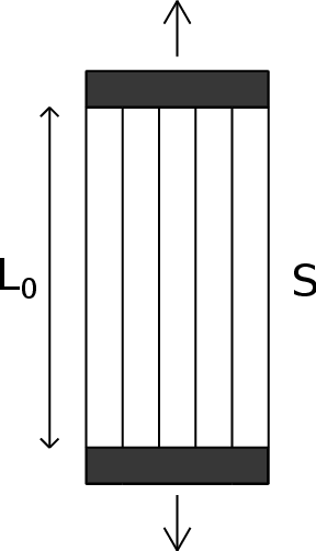
Figure 1: Idealized material for the description of the uniaxial damage theory.

For the present purpose, the material is idealized as a bundle of fibers parallel to the loading direction (Figure 1). Initially, all the fibers respond elastically, and the stress is carried by the total cross section of all fibers ${\textstyle S}$ (Figure 2.1). As the applied strain is increased some fibers start breaking (Figure 2.2). Each fiber is assumed to be perfectly brittle, meaning that the stress in the fiber drops down to zero immediately after a critical strain level is reached. However, since the critical strain can differ from one fiber to another, the effective area ${\textstyle {\bar {S}}}$ (the area of unbroken fibers that can still carry stress) will decrease gradually from ${\textstyle {\bar {S}}=S}$ to ${\textstyle {\bar {S}}=0}$. Of course, when the applied force diminishes (Figure 3.2), the affected fibers remain broken and so the damaged area of the specimen is irrecoverable.

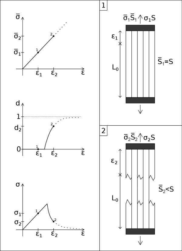
Figure 2: Scheme of a uniaxial damage model through a monotonic loading process.

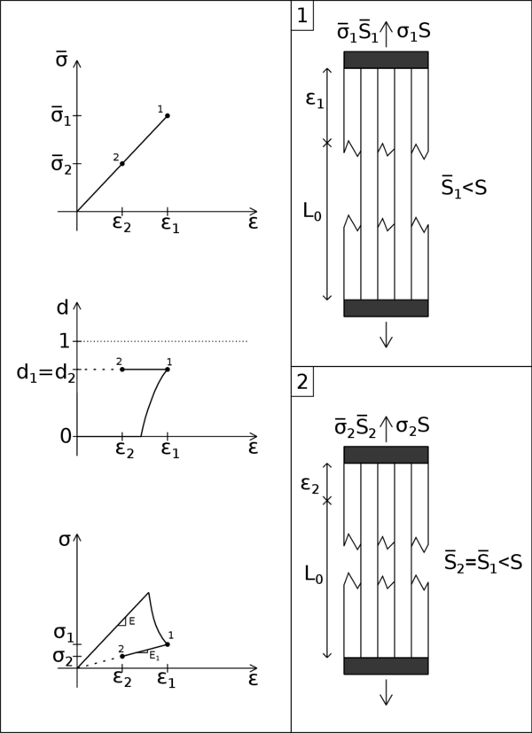
Figure 3: Scheme of a uniaxial damage model through a non-monotonic loading process.

It is important to make a distinction between the nominal stress ${\textstyle \sigma }$, defined as the force per unit initial area of the cross section, and the effective stress ${\textstyle {\bar {\sigma }}}$, defined as the force per unit effective area. The nominal stress enters the Cauchy equations of equilibrium on the macroscopic level, while the effective stress is the "actual" stress acting in the material micro-structure. From the condition of equivalence, ${\textstyle \sigma S={\bar {\sigma }}{\bar {S}}}$, we obtain:

$\sigma ={\frac {\bar {S}}{S}}{\bar {\sigma }}$

(1)

The ratio of the effective area to the total area, ${\textstyle {\bar {S}}/S}$, is a scalar characterizing the integrity of the material. Within the classical approach, a very simple measure of the damage amplitude in a given plane is obtained by measuring the area of the intersection of all defects with that plane. Thereby, we can define the damage parameter as:

$d=1-{\frac {\bar {S}}{S}}={\frac {S-{\bar {S}}}{S}}={\frac {S_{d}}{S}}$

(2)

where ${\textstyle S_{d}=S-{\bar {S}}}$ is the damaged part of the area. An undamaged material is characterized then by ${\textstyle {\bar {S}}=S}$, i.e., by ${\textstyle d=0}$. Due to propagation of micro-defects and their coalescence, the damage variable grows and at the late stages of degradation process it approaches asymptotically the limit value ${\textstyle d=1}$, corresponding to a complete damaged material with effective area reduced to zero.

In the simplest version of the presented scheme, each fiber is supposed to remain linear elastic up to the strain level at which it breaks. Consequently, the 1D effective stress ${\textstyle {\bar {\sigma }}}$ is related to the elastic strain of the material ${\textstyle \varepsilon }$ by the uniaxial Hooke's law:

${\bar {\sigma }}=E\varepsilon$

(3)

where E is the elastic modulus of the undamaged material. Combining (1), (2) and (3), it is easily seen that the constitutive law for the nominal stress ${\textstyle \sigma }$ takes the form:

$\sigma =(1-d)E\varepsilon$

(4)

For the uniaxial model formulation, equation (4) must be complemented with the damage evolution law, which can be characterized by the dependence between the damage variable and the applied strain:

${\begin{array}{cc}d=g(\varepsilon )&\quad 0\leq d\leq 1\end{array}}$

(5)

Function ${\textstyle g}$ affects the shape of the stress-strain diagram and can be directly identified from a uniaxial test.

The evolution of the effective stress, damage variable, and nominal stress in a material that remains elastic up to the peak stress is shown in Figure 2. This description is valid only for monotonic loading by an increasing applied strain ${\textstyle \varepsilon }$. When the material is first stretched up to a certain strain level ${\textstyle \varepsilon _{1}}$ that induces damage ${\textstyle d_{1}=g(\varepsilon _{1})}$ and then the strain decreases (Figure 3), the damaged area remains constant and the material responds as an elastic material with a reduced Young's modulus ${\textstyle E_{1}=(1-d_{1})E}$. This means that, during unloading and partial reloading, the damage variable in (4) must be evaluated from the largest previously reached strain and not from the current strain ${\textstyle \varepsilon }$. This means that it is crucial to introduce an internal state variable ${\textstyle r}$ characterizing the maximum strain level reached in the previous history of the material up to a given time ${\textstyle t}$:

$r(t)=\max \left\{r_{0},\max _{\tau \leq t}\varepsilon (\tau )\right\}$

(6)

The expression implies that ${\textstyle r(t)\geq r_{0}}$, where ${\textstyle r_{0}}$ is the so-called damage threshold, a material parameter that represents the value of strain at which damage starts. In this formula, ${\textstyle t}$ is not necessarily the physical time (it can be any monotonically increasing parameter controlling the loading process). The damage evolution law (5) is then rewritten in the form:

$d=g(r){\hbox{ with }}\left\{{\begin{array}{cc}g(r)=0&{\hbox{if }}r=r_{0}{\hbox{ }}\\0<g(r)\leq {1}&{\hbox{if }}r>r_{0}{\hbox{ }}\end{array}}\right.$

(7)

which remains valid not only during monotonic loading but also during unloading and reloading. The evolution of the effective stress, damage variable, and nominal stress in a non-monotonic test is shown in Figure 3. Note that, upon a complete removal of the applied force, the strain returns to zero (due to elasticity of the unbroken fibers), i.e., the pure damage model does not take into account any permanent strains. Nevertheless, the material state will be different from the initial virgin state because, according to (6) and (7), when the state variable ${\textstyle r}$ becomes greater than ${\textstyle r_{0}}$, the damage variable will not be zero again, thus the stiffness and strength mobilized in a new tensile loading process will be smaller than their initial values. Therefore, we can say that the loading history is always reflected by the value of the internal state variable ${\textstyle r}$.

To gain further insight, we can rewrite the constitutive law (4) in the form ${\textstyle \sigma =E_{sec}\varepsilon }$ where ${\textstyle E_{sec}=(1-d)E}$ is the apparent or damaged modulus of elasticity. Furthermore, instead of defining the variable ${\textstyle r}$ like (6), we can introduce a loading function ${\textstyle f(\varepsilon ,r)=\varepsilon {-}r}$ and postulate the loading-unloading conditions in the Kuhn-Tucker form:

${\begin{array}{ccc}f\leq {0};&{\dot {r}}\geq {0};&{\dot {r}}f=0\end{array}}$

(8)

The first condition indicates that ${\textstyle r}$ can never be smaller than ${\textstyle \varepsilon }$, while the second condition means that ${\textstyle r}$ cannot decrease. Finally, according to the third condition, ${\textstyle r}$ can grow only if the current values of ${\textstyle \varepsilon }$ and ${\textstyle r}$ are equal.

At this point, we can already summarize the basic components of the uniaxial damage theory:

• The stress-strain law in the secant format:

$\sigma =E_{sec}\varepsilon$

(9)

with:

$E_{sec}=(1-d)E$

(10)

• The law governing the evolution of the damage variable (7)
• The damage criterion, comprising:

• The loading function:

$f(\varepsilon ,r)=\varepsilon {-}r$

(11)

specifying the elastic domain ${\textstyle {\mathcal {E}}_{r}=\{\varepsilon |f(\varepsilon ,r)<0\}}$, i.e., the set of states for which damage does not grow.

• The loading-unloading conditions (8)

2.2.2 A simple isotropic damage theory

The simplest extension of the uniaxial damage theory to general multiaxial stress states is achieved by the isotropic damage model with a unique scalar variable. Isotropic damage models are based on the simplifying assumption that the stiffness degradation is isotropic, i.e., the stiffness moduli corresponding to different directions decrease proportionally, independently of the direction of loading. Since an isotropic elastic material is characterized by two independent elastic constrains, a general isotropic damage model should deal with two damage variables. The model with a single variable makes use of the additional assumption that the relative reduction of all the stiffness coefficients is the same, in other words, that the Poisson's ratio is not affected by damage. In this regard, the damaged constitutive tensor is expressed as:

${\boldsymbol {E}}_{sec}=(1-d){\boldsymbol {E}}$

(12)

where ${\textstyle {\boldsymbol {E}}}$ is the elastic constitutive tensor of the intact material, and ${\textstyle d}$ is the damage variable. In the present context, ${\textstyle {\boldsymbol {E}}_{sec}}$ is the secant constitutive tensor that relates the total strain ${\textstyle {\boldsymbol {\varepsilon }}}$ to the total stress ${\textstyle {\boldsymbol {\sigma }}}$, according to:

${\boldsymbol {\sigma }}={\boldsymbol {E}}_{sec}:{\boldsymbol {\varepsilon }}=(1-d){\boldsymbol {E}}:{\boldsymbol {\varepsilon }}$

(13)

One can clearly notice that (12) is a generalization of (10), and (13) is a generalization of (9) and (4). Furthermore, equation (13) can alternatively be written as:

${\boldsymbol {\sigma }}=(1-d){\boldsymbol {\bar {\sigma }}}$

(14)

which is the multidimensional generalization of (1), and where ${\textstyle {\boldsymbol {\bar {\sigma }}}}$ is the effective stress tensor defined as:

${\boldsymbol {\bar {\sigma }}}={\boldsymbol {E}}:{\boldsymbol {\varepsilon }}$

(15)

Similar to the uniaxial case, we introduce a loading function ${\textstyle f}$ specifying the elastic domain and the states at which damage grows. The loading function now depends on the strain tensor ${\textstyle {\boldsymbol {\varepsilon }}}$, and on a variable ${\textstyle r}$ that controls the evolution of the elastic domain. Physically. ${\textstyle r}$ represents a scalar measure of the largest strain level ever reached in the history of the material. States for which ${\textstyle f({\boldsymbol {\varepsilon }},r)<0}$ are supposed to be below the current damage threshold. Damage can grow only if the current state reaches the boundary of the elastic domain, i.e., when ${\textstyle f({\boldsymbol {\varepsilon }},r)=0}$. Essentially, we can postulate the damage criterion for a multiaxial isotropic damage model with:

• The loading function:

$f({\boldsymbol {\varepsilon }},r)=\varepsilon _{eq}({\boldsymbol {\varepsilon }})-r$

(16)

• The loading-unloading conditions (8)

where ${\textstyle \varepsilon _{eq}}$ is the equivalent strain, i.e., a scalar measure of the strain level, and ${\textstyle r}$ is the largest value of equivalent strain calculated in the previous deformation history of the material up to its current state. In this regard, (6) can now be generalized to:

$r(t)=\max \left\{r_{0},\max _{\tau \leq t}\varepsilon _{eq}(\tau )\right\}$

(17)

An important advantage of an isotropic damage model is that the stress evaluation algorithm is usually explicit and there is no need to use an iterative solution for non-linear equations.

Thereby, for a particular strain increment, the corresponding stress is obtained by computing the current value of equivalent strain, updating the maximum previously reached equivalent strain and the damage variable, and reducing the effective stress according to (13). In essence, one must follow the scheme of Table 1:

Table. 1 Isotropic damage model scheme.

Input data for time $t+1$: ${\boldsymbol {E}}$, ${\boldsymbol {\varepsilon }}^{t}$, $\Delta {\boldsymbol {\varepsilon }}$, $r^{t}$

1. Determine new strain vector: ${\textstyle {\boldsymbol {\varepsilon }}^{t+1}={\boldsymbol {\varepsilon }}^{t}+\Delta {\boldsymbol {\varepsilon }}}$

2. Evaluate effective stresses: ${\textstyle {\boldsymbol {\bar {\sigma }}}^{t+1}={\boldsymbol {E}}:{\boldsymbol {\varepsilon }}^{t+1}}$

3. Compute equivalent strain from the new strain vector: ${\textstyle \varepsilon _{eq}^{t+1}}$

4. Update ${\textstyle r}$ with (17): If ${\textstyle (\varepsilon _{eq}^{t+1}>r^{t})\Rightarrow r^{t+1}=\varepsilon _{eq}^{t+1}}$

5. Update damage variable: ${\textstyle d^{t+1}=g(r^{t+1})}$

6. Compute stresses: ${\textstyle {\boldsymbol {\sigma }}^{t+1}=(1-d^{t+1}){\boldsymbol {\bar {\sigma }}}^{t+1}}$

2.2.2.1 Equivalent strain forms

To some extent, the expression defining the equivalent strain plays a role similar to the yield function in plasticity, because it directly affects the shape of the elastic domain (Figure 4).

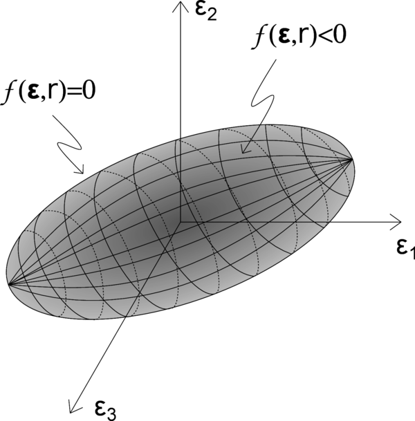
Figure 4: 3D elastic domain for a generic equivalent strain.

There are numerous forms of equivalent strain in the literature, but the simplest choice is to define it as the Euclidean norm of the strain tensor:

$\varepsilon _{eq}=\|{\boldsymbol {\varepsilon }}\|={\sqrt {{\boldsymbol {\varepsilon }}:{\boldsymbol {\varepsilon }}}}={\sqrt {\varepsilon _{ij}\varepsilon _{ij}}}$

(18)

or as the energy norm:

$\varepsilon _{eq}={\sqrt {\frac {{\boldsymbol {\varepsilon }}:{\boldsymbol {E}}:{\boldsymbol {\varepsilon }}}{E}}}={\sqrt {{\frac {1}{E}}E_{ijkl}\varepsilon _{ij}\varepsilon _{kl}}}$

(19)

where ${\textstyle E_{ijkl}}$ are the components of the elastic constitutive tensor ${\textstyle {\boldsymbol {E}}}$ and normalization by Young's modulus ${\textstyle E}$ is introduced to obtain a strain-like quantity.

The two norms of ${\textstyle {\boldsymbol {\varepsilon }}}$ introduced above, lead to symmetric elastic domain in tension and compression. Nevertheless, several materials (rocks, concrete, ceramics, etc.) often show a non symmetric damage surface, i.e., the yield value in compression can be several times the value in tension. In order to overcome this limitation, it is necessary to adjust the definition of the equivalent strain.

Micro-cracks in concrete grow mainly if the material is stretched, and so it is natural to take into account only normal strains that are positive (tensile strains) and neglect those that are negative (compressive strains). This leads to the so-called Mazars definition of equivalent strains [31]:

$\varepsilon _{eq}=\|\langle {\boldsymbol {\varepsilon }}\rangle \|={\sqrt {\langle {\boldsymbol {\varepsilon }}\rangle :\langle {\boldsymbol {\varepsilon }}\rangle }}$

(20)

or to its energetic counterpart:

$\varepsilon _{eq}={\sqrt {\frac {\langle {\boldsymbol {\varepsilon }}\rangle :{\boldsymbol {E}}:\langle {\boldsymbol {\varepsilon }}\rangle }{E}}}$

(21)

where McAuley brackets ${\textstyle \langle .\rangle }$ denote the "positive part" operator. For scalars ${\textstyle \langle x\rangle =\max(0,x)}$, i.e.,

$\langle x\rangle =\left\{{\begin{array}{ll}x&{\hbox{if }}x>0{\hbox{ }}\\0&{\hbox{if }}x\leq {\hbox{ 0 }}\end{array}}\right.$

(22)

For symmetric tensors, such as the strain tensor ${\textstyle {\boldsymbol {\varepsilon }}}$, the positive part is a tensor with the same principal directions ${\textstyle {\boldsymbol {n_{i}}}}$ as the original one, but replacing its principal values ${\textstyle \varepsilon _{i}}$ by their positive parts ${\textstyle \langle \varepsilon _{i}\rangle }$. The subscript ${\textstyle i}$ ranges from 1 to 3 (the number of spatial dimensions). If we consider the following diagonalized strain tensor:

${\boldsymbol {\varepsilon }}={\begin{bmatrix}\varepsilon _{1}&0&0\\0&\varepsilon _{2}&0\\0&0&\varepsilon _{3}\end{bmatrix}}$

(23)

the positive part of ${\textstyle {\boldsymbol {\varepsilon }}}$ is expressed as:

$\langle {\boldsymbol {\varepsilon }}\rangle ={\begin{bmatrix}\langle \varepsilon _{1}\rangle &0&0\\0&\langle \varepsilon _{2}\rangle &0\\0&0&\langle \varepsilon _{3}\rangle \end{bmatrix}}$

(24)

Thereby, knowing that ${\textstyle \langle {\boldsymbol {\varepsilon }}\rangle :\langle {\boldsymbol {\varepsilon }}\rangle =tr(\langle {\boldsymbol {\varepsilon }}\rangle ^{T}\langle {\boldsymbol {\varepsilon }}\rangle )}$, definition (20) can be rewritten as:

$\varepsilon _{eq}={\sqrt {\sum _{i=1}^{3}\langle \varepsilon _{i}\rangle ^{2}}}$

(25)

An alternative formula, called the modified von Mises definition [32], reads:

$\varepsilon _{eq}={\frac {\kappa {-1}}{2\kappa (1-2\nu )}}I_{1}+{\frac {1}{2\kappa }}{\sqrt {\left({\frac {\kappa {-1}}{1-2\nu }}I_{1}\right)^{2}+{\frac {12\kappa }{(1+\nu )^{2}}}J_{2}}}$

(26)

where ${\textstyle \kappa }$ is a model parameter that sets the ratio between the uniaxial compressive strength and the uniaxial tensile strength, ${\textstyle \nu }$ is the Poisson's ratio of the material, ${\textstyle I_{1}}$ is the first invariant of the strain tensor, and ${\textstyle J_{2}}$ is the second invariant of the deviatoric strain tensor. Given a generic symmetric strain tensor ${\textstyle {\boldsymbol {\varepsilon }}}$:

${\boldsymbol {\varepsilon }}={\begin{bmatrix}\varepsilon _{xx}&\varepsilon _{xy}&\varepsilon _{xz}\\\varepsilon _{xy}&\varepsilon _{yy}&\varepsilon _{yz}\\\varepsilon _{xz}&\varepsilon _{yz}&\varepsilon _{zz}\end{bmatrix}}$

(27)

The first invariant ${\textstyle I_{1}}$ is the trace of the strain tensor:

$I_{1}=tr({\boldsymbol {\varepsilon }})=\varepsilon _{xx}+\varepsilon _{yy}+\varepsilon _{zz}$

(28)

One can always decompose the strain tensor into its volumetric and deviatoric parts ${\textstyle {\boldsymbol {\varepsilon }}={\boldsymbol {\varepsilon }}_{v}+{\boldsymbol {\varepsilon }}_{d}}$:

${\boldsymbol {\varepsilon }}_{v}={\begin{bmatrix}{\frac {I_{1}}{3}}&0&0\\0&{\frac {I_{1}}{3}}&0\\0&0&{\frac {I_{1}}{3}}\end{bmatrix}}$

(29)

${\boldsymbol {\varepsilon }}_{d}={\begin{bmatrix}\varepsilon _{xx}-{\frac {I_{1}}{3}}&\varepsilon _{xy}&\varepsilon _{xz}\\\varepsilon _{xy}&\varepsilon _{yy}-{\frac {I_{1}}{3}}&\varepsilon _{yz}\\\varepsilon _{xz}&\varepsilon _{yz}&\varepsilon _{zz}-{\frac {I_{1}}{3}}\end{bmatrix}}$

(30)

From the deviatoric strain tensor ${\textstyle {\boldsymbol {\varepsilon }}_{d}}$ we can calculate ${\textstyle J_{1}}$ and ${\textstyle J_{2}}$:

$J_{1}=tr({\boldsymbol {\varepsilon }}_{d})=\varepsilon _{xx}-{\frac {I_{1}}{3}}+\varepsilon _{yy}-{\frac {I_{1}}{3}}+\varepsilon _{zz}-{\frac {I_{1}}{3}}=I_{1}-3{\frac {I_{1}}{3}}=0$

(31)

$J_{2}$ $={\frac {1}{2}}({\boldsymbol {\varepsilon }}_{d}:{\boldsymbol {\varepsilon }}_{d}-J_{1}^{2})={\frac {1}{2}}({\boldsymbol {\varepsilon }}_{d}:{\boldsymbol {\varepsilon }}_{d})$ $={\frac {1}{3}}\left[\varepsilon _{xx}^{2}+\varepsilon _{yy}^{2}+\varepsilon _{zz}^{2}-\varepsilon _{xx}\varepsilon _{yy}-\varepsilon _{xx}\varepsilon _{zz}-\varepsilon _{yy}\varepsilon _{zz}\right]+$ $\varepsilon _{xy}^{2}+\varepsilon _{xz}^{2}+\varepsilon _{yz}^{2}$

(32)

Another possibility is to work with an evolution of the model proposed by Simo and Ju [23], using the energy norm of the strain tensor and modifying it to take into account the different degradation in tension and compression of concrete-like materials. In this case, the equivalent strain takes the form:

$\varepsilon _{eq}=\left(\theta +{\frac {1-\theta }{\kappa }}\right){\sqrt {{\boldsymbol {\varepsilon }}:{\boldsymbol {E}}:{\boldsymbol {\varepsilon }}}}$

(33)

where the parameter ${\textstyle \theta }$ is a weighting factor depending on the effective stresses ${\textstyle {\bar {\boldsymbol {\sigma }}}}$, given by:

$\theta ={\frac {\sum _{i=1}^{3}\langle {\bar {\sigma }}_{i}\rangle }{\sum _{i=1}^{3}|{\bar {\sigma }}_{i}|}}$

(34)

As mentioned before, the parameter ${\textstyle \kappa }$ is defined by means of the ratio between the compression elastic limit ${\textstyle \sigma _{y}^{c}}$ and the tension elastic limit ${\textstyle \sigma _{y}^{t}}$, i.e.:

$\kappa ={\frac {\sigma _{y}^{c}}{\sigma _{y}^{t}}}$

(35)

In the case of concrete ${\textstyle \kappa \approx {10}}$.

The equivalent strains presented in this subsection lead to different damage surfaces but all three share a common trait, the elastic limit in tension ${\textstyle \sigma _{y}^{t}}$ is much lower than the elastic limit in compression ${\textstyle \sigma _{y}^{c}}$ (Figure 5.b, 5.c, 5.d). In contrast, the equivalent strain obtained from the original energy norm definition (19) leads to a symmetric damage surface in which there is no difference between the elastic limit in tension and compression (Figure 5.a).

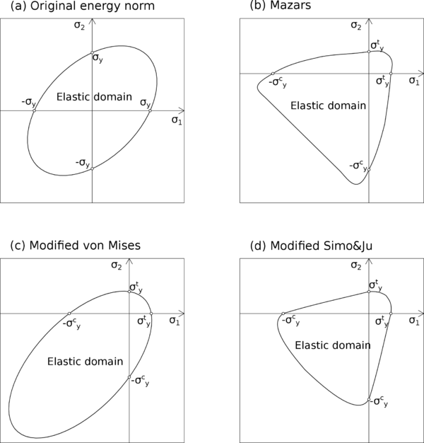
Figure 5: Damage surfaces for different equivalent strains in the 2D principal stress space.

2.2.3 Damage evolution laws

As we stated for the uniaxial case, one of the basic components of a damage model is the law governing the evolution of the damage variable (7). There are various damage governing laws ${\textstyle g(r)}$ that can be effectively used to model damage growth in geo-materials, and in the following lines we will present some of the most widely used options.

Two typical choices to describe the evolution of damage above the damage threshold ${\textstyle r_{0}}$ are the exponential law [20]:

$g(r)=1-{\frac {r_{0}(1-A)}{r}}-A\exp\{-B(r-r_{0})\}$

(36)

and the polynomial law [33]:

$g(r)=1-{\frac {1}{1+B(r-r_{0})+A(r-r_{0})^{2}}}$

(37)

In (36) and (37) parameter ${\textstyle A}$ is associated to residual strength and parameter ${\textstyle B}$ controls the slope of the softening branch at the peak of the stress-strain curve.

Another option, especially suited for simplified analyses, is the linear softening law. Limiting the state variable ${\textstyle r}$ between the damage threshold ${\textstyle r_{0}}$ and a maximum admissible value ${\textstyle r_{max}}$, damage evolves according to:

$g(r)={\frac {r_{max}}{r_{max}-r_{0}}}\left(1-{\frac {r_{0}}{r}}\right)$

(38)

which leads to a linear softening branch in the stress-strain curve.

The effect of using one form of damage evolution law or another is clearly seen in a uniaxial case. Figure 6 shows the aspect of the stress-strain curve in a unidimensional case using the three softening laws presented above. For all three cases we have used a damage threshold of ${\textstyle r_{0}=2\cdot {10}^{-4}}$ and a Young's modulus of ${\textstyle E=28000}$ MPa. The exponential law is represented with ${\textstyle A=0.8}$ and ${\textstyle B=15000}$, the polynomial law with ${\textstyle A=0.8}$ and ${\textstyle B=30000}$, and for the linear law we have defined ${\textstyle r_{max}=5\cdot {10}^{-4}}$. One can see that when the strain exceeds the damage threshold after the elastic branch ${\textstyle \varepsilon {>}r_{0}}$, a softening post-peak branch starts as a result of the damage growing.

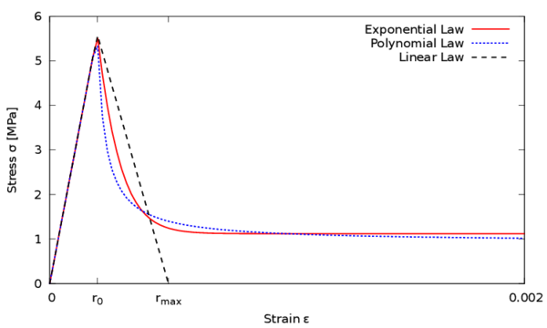
Figure 6: Unidimensional stress-strain curves for different damage evolution laws.

An alternative exponential softening model was proposed in [27]:

$g(r)=1-{\frac {r_{0}}{r}}\exp \left\{A_{f}\left(1-{\frac {r}{r_{0}}}\right)\right\}$

(39)

The parameter ${\textstyle A_{f}}$ is obtained from the following expression:

$A_{f}=\left({\frac {G_{f}}{l_{f}(r_{0})^{2}}}-{\frac {1}{2}}\right)^{-1}\geq 0$

(40)

where ${\textstyle G_{f}}$ is the specific fracture energy per unit area, ${\textstyle l_{f}}$ is the characteristic length for the fractured domain, usually taken as the characteristic length of the finite elements, and ${\textstyle r_{0}}$ is the damage threshold which, for the Simo and Ju model, can be computed from:

$r_{0}={\frac {\sigma _{y}^{t}}{\sqrt {E}}}$

(41)

being ${\textstyle \sigma _{y}^{t}}$ the tensile strength of the material, and ${\textstyle E}$ the Young's modulus.

Another popular damage evolution law specifically designed for concrete was proposed by Mazars [31,20]. He introduced two damage variables, ${\textstyle d_{c}}$ and ${\textstyle d_{t}}$, that are computed from the same equivalent strain (25) using two different damage functions, ${\textstyle g_{c}}$ and ${\textstyle g_{t}}$. Function ${\textstyle g_{c}}$ is identified from the uniaxial compressive test while ${\textstyle g_{t}}$ corresponds to the tensile test. The evolution law governing damage ${\textstyle g(r)}$ results from the combination of the two parts:

$g(r)=\alpha _{t}^{\beta }g_{t}(r)+(1-\alpha _{t})^{\beta }g_{c}(r)$

(42)

Functions characterizing the evolution of damage in compression ${\textstyle g_{c}}$ and in tension ${\textstyle g_{t}}$ were proposed in the exponential form:

$g_{c}(r)=1-{\frac {r_{0}(1-A_{c})}{r}}-A_{c}\exp\{-B_{c}(r-r_{0})\}$

(43)

$g_{t}(r)=1-{\frac {r_{0}(1-A_{t})}{r}}-A_{t}\exp\{-B_{t}(r-r_{0})\}$

(44)

where ${\textstyle A_{c}}$, ${\textstyle B_{c}}$, ${\textstyle A_{t}}$, ${\textstyle B_{t}}$ are material parameters related to the shape of uniaxial stress-strain diagrams.

The coefficient ${\textstyle \alpha _{t}}$ in (42) ranges from 0 to 1 and takes into account the character of the stress state. It is evaluated from:

$\alpha _{t}=\sum _{i=1}^{3}{\frac {\varepsilon _{ti}\langle \varepsilon _{i}\rangle }{\varepsilon _{eq}^{2}}}$

(45)

where ${\textstyle \varepsilon _{ti}}$ are the principal strains due to positive effective stresses, i.e., the principal values of ${\textstyle {\boldsymbol {\varepsilon }}_{t}={\boldsymbol {E}}^{-1}:\langle {\boldsymbol {E}}:{\boldsymbol {\varepsilon }}\rangle }$:

${\boldsymbol {\varepsilon }}_{t}=-{\frac {\nu }{E}}tr(\langle {\boldsymbol {\bar {\sigma }}}\rangle ){\boldsymbol {I}}+{\frac {1+\nu }{E}}\langle {\boldsymbol {\bar {\sigma }}}\rangle$

(46)

being ${\textstyle {\boldsymbol {I}}}$ the identity tensor.

The parameter ${\textstyle \beta }$ in (42) was equal to 1 in the original version of the model [31]. When it is higher than 1, ${\textstyle \beta }$ allows to slow down the evolution of damage under shear loading (when principal stresses have different sign).

The definition of ${\textstyle \varepsilon _{ti}}$ tells us that if all principal stresses are negative then ${\textstyle \alpha _{t}=0}$ and ${\textstyle d=d_{c}=g_{c}(r)}$, and if all principal stresses are positive we have ${\textstyle \alpha _{t}=1}$ and ${\textstyle d=d_{t}=g_{t}(r)}$. These are the "purely compressive" and "purely tensile" stress states. For intermediate stress states the value of ${\textstyle d}$ is between ${\textstyle d_{c}}$ and ${\textstyle d_{t}}$, depending on the relative magnitudes of tensile and compressive stresses.

2.2.4 Elastic-damage tangent constitutive tensor

In this section we will present the tangent constitutive tensor, which gives us an important advantage, from a computational point of view, when dealing with incremental iterative solution procedures. Basically, with the tangent constitutive tensor one can achieve a quadratic convergence rate, whereas with the secant constitutive tensor, the solution is limited to a linear convergence.

The damaged or secant constitutive tensor ${\textstyle {\boldsymbol {E}}_{sec}}$ introduced in (12) and (13) links the total stress to total strain and plays the role of the tangent stiffness only for processes with elastic loading or unloading with constant damage (${\textstyle f<0}$). To obtain the tangent stiffness for a loading process with growing damage (${\textstyle f=0}$ and ${\textstyle {\dot {f}}=0}$), it is necessary to find the link between stress and strain increments. This concepts are clearly seen in a unidimensional case (see Figure 7). In this regard, knowing the difference between secant and tangent moduli (see Figure 8.a and 8.b) is useful to understand the generalization to secant and tangent constitutive tensors.

Figure 7: Uniaxial stress-strain diagram of a loading-unloading process.

Figure 8: Secant and tangent moduli.

In essence, we define the elastic-damage tangent constitutive tensor ${\textstyle {\boldsymbol {E}}_{tan}}$ as the one that satisfies the following relation:

${\dot {\boldsymbol {\sigma }}}={\boldsymbol {E}}_{tan}:{\dot {\boldsymbol {\varepsilon }}}$

(47)

Now, by considering the equation (13), we can obtain the rate of change of stress as follows:

${\dot {\boldsymbol {\sigma }}}({\boldsymbol {\varepsilon }},d)$ $={\frac {\partial {\boldsymbol {\sigma }}}{\partial {\boldsymbol {\varepsilon }}}}:{\dot {\boldsymbol {\varepsilon }}}+{\frac {\partial {\boldsymbol {\sigma }}}{\partial d}}{\dot {d}}=(1-d){\boldsymbol {E}}:{\dot {\boldsymbol {\varepsilon }}}-{\boldsymbol {E}}:{\boldsymbol {\varepsilon }}{\dot {d}}$ $=(1-d){\boldsymbol {E}}:{\dot {\boldsymbol {\varepsilon }}}-{\bar {\boldsymbol {\sigma }}}\otimes {\dot {d}}$

(48)

from which we should distinguish two possible situations:

1. A process with elastic loading or unloading (${\textstyle {\dot {r}}=0\Rightarrow {\dot {d}}=0}$)

With ${\textstyle {\dot {d}}=0}$ equation (48) becomes ${\textstyle {\dot {\boldsymbol {\sigma }}}=(1-d){\boldsymbol {E}}:{\dot {\boldsymbol {\varepsilon }}}}$, from which we obtain that the elastic-damage tangent constitutive tensor coincides with the secant constitutive tensor:

${\boldsymbol {E}}_{tan}={\boldsymbol {E}}_{sec}=(1-d){\boldsymbol {E}}$

(49)

2. A loading process with growing damage (${\textstyle {\dot {r}}>0\Rightarrow {\dot {d}}>0}$)

In this case, in order to obtain an explicit expression of the tangent constitutive tensor, the damage rate ${\textstyle {\dot {d}}}$ should be expressed in terms of the strain rate ${\textstyle {\dot {\boldsymbol {\varepsilon }}}}$. This can be achieved by imposing the consistency condition ${\textstyle {\dot {f}}=0}$ in equation (16) and combining it with the rate of equation (7):

${\dot {d}}={\frac {dg}{dr}}{\dot {r}}={\frac {dg}{dr}}{\dot {\varepsilon }}_{eq}={\frac {dg}{dr}}{\frac {\partial \varepsilon _{eq}}{\partial {\boldsymbol {\varepsilon }}}}:{\dot {\boldsymbol {\varepsilon }}}$

(50)

For convenience, we introduce symbols ${\textstyle g'}$ for the derivative of the damage function ${\textstyle dg/dr}$, and ${\textstyle {\boldsymbol {\eta }}}$ for the second order tensor obtained from the partial derivative of the equivalent strain with respect to the strain tensor ${\textstyle \partial \varepsilon _{eq}/\partial {\boldsymbol {\varepsilon }}}$. Thereby, substituting ${\textstyle {\dot {d}}=g'{\boldsymbol {\eta }}:{\dot {\boldsymbol {\varepsilon }}}}$ into the rate of change of stress (48), we get:

${\dot {\boldsymbol {\sigma }}}=(1-d){\boldsymbol {E}}:{\dot {\boldsymbol {\varepsilon }}}-{\bar {\boldsymbol {\sigma }}}\otimes (g'{\boldsymbol {\eta }}:{\dot {\boldsymbol {\varepsilon }}})=[(1-d){\boldsymbol {E}}-g'{\bar {\boldsymbol {\sigma }}}\otimes {\boldsymbol {\eta }}]:{\dot {\boldsymbol {\varepsilon }}}$

(51)

and, consequently, the elastic-damage constitutive tensor results:

${\boldsymbol {E}}_{tan}=(1-d){\boldsymbol {E}}-g'{\bar {\boldsymbol {\sigma }}}\otimes {\boldsymbol {\eta }}$

(52)

where the form of ${\textstyle g'}$ and ${\textstyle {\boldsymbol {\eta }}}$ depend on the damage evolution law, and on the equivalent strain expression chosen for the damage model.

For instance, for a model with an equivalent strain ${\textstyle \varepsilon _{eq,1}}$ based on the energy norm of equation (19), tensor ${\textstyle {\boldsymbol {\eta }}_{1}}$ is given by:

${\boldsymbol {\eta }}_{1}={\frac {\partial \varepsilon _{eq,1}}{\partial {\boldsymbol {\varepsilon }}}}={\frac {1}{2{\sqrt {\frac {{\boldsymbol {\varepsilon }}:{\boldsymbol {E}}:{\boldsymbol {\varepsilon }}}{E}}}}}{\frac {1}{E}}2{\boldsymbol {E}}:{\boldsymbol {\varepsilon }}={\frac {\bar {\boldsymbol {\sigma }}}{E\varepsilon _{eq,1}}}$

(53)

and the resulting tangent constitutive tensor for this particular case is:

${\boldsymbol {E}}_{tan,1}=(1-d){\boldsymbol {E}}-{\frac {g'}{E\varepsilon _{eq,1}}}{\bar {\boldsymbol {\sigma }}}\otimes {\bar {\boldsymbol {\sigma }}}$

(54)

which preserves symmetry (${\textstyle {\boldsymbol {E}}_{tan,1}^{T}={\boldsymbol {E}}_{tan,1}}$). It must be noticed though that, for other definitions of equivalent strain, this kind of symmetry is lost.

The typical scheme for the numerical implementation of the elastic-damage tangent constitutive tensor is shown in Table (2).

Table. 2 Flowchart for the numerical implementation of the elastic-damage tangent constitutive tensor.

Input data for time $t+1$: ${\boldsymbol {E}}$, ${\bar {\boldsymbol {\sigma }}}^{t+1}$, $r^{t}$, $r^{t+1}$, $d^{t+1}$
If (${\textstyle r^{t+1}>r^{t}}$)	Loading with growing damage (${\textstyle {\dot {r}}>0\Rightarrow {\dot {d}}>0}$):
	1. Compute damage function derivative:
	$g'=dg/dr$
	2. Calculate equivalent strain partial derivative:
	${\boldsymbol {\eta }}=\partial \varepsilon _{eq}/\partial {\boldsymbol {\varepsilon }}$
	3. Compute tangent constitutive tensor with (52):
	${\boldsymbol {E}}_{tan}^{t+1}=(1-d^{t+1}){\boldsymbol {E}}-g'{\bar {\boldsymbol {\sigma }}}^{t+1}\otimes {\boldsymbol {\eta }}$
Else	Elastic loading or unloading (${\textstyle {\dot {r}}=0\Rightarrow {\dot {d}}=0}$):
	${\boldsymbol {E}}_{tan}^{t+1}={\boldsymbol {E}}_{sec}^{t+1}=(1-d^{t+1}){\boldsymbol {E}}$

2.3 Local and Non-local Damage Models

In previous sections we have presented the basic ideas of isotropic damage models with a unique scalar variable ${\textstyle d}$. Although these models are quite simple, they are often used to model the failure of concrete and other quasi-brittle materials that show important strain localization. If the damage parameter depends only on the strain state at the point under consideration, the numerical simulations exhibit a pathological mesh dependence, and physically unrealistic results are obtained.

This is the typical behaviour of the so-called local damage models, which are not able to properly describe both the thickness of localization and distance between them. They suffer from mesh sensitivity (for size and alignment) and produce unreliable results. The strains concentrate in one element wide zones and the computed force-displacement curves are mesh-dependent. The reason is that differential equations of motion change their type (from elliptic to hyperbolic in static problems) and the rate boundary value problem becomes ill-posed.

Thus, classical constitutive models require an extension in the form of a characteristic length to properly model the thickness of localized zones. Such extension can be done with micro-polar [34,35], strain gradient [36,37,38], viscous [39,40,41] and non-local terms [42,43,44,45]. In this work we have developed the latter approach.

Similarly to previous sections, in order to make it more understandable, we will present the inconveniences arisen due to strain localization with a uniaxial example. After that, the basic concepts of the implemented non-local damage model will be stated.

2.3.1 Strain localization phenomenon

The idea of modelling damaged concrete and other quasi-brittle materials as strain-softening continua, was not immediately accepted by all the scientific community. Actually, most of the early analyses were not truly objective and, upon mesh refinement, their results would not converge to a robust solution. Let us explain the nature of the problem by means of a unidimensional example.

Consider a straight bar with a constant cross section ${\textstyle S}$ and a total length ${\textstyle L_{0}}$ under uniaxial tension (Figure 9). The material is assumed to obey a simple stress-strain law with linear elasticity up to the peak stress ${\textstyle \sigma _{y}}$, followed by linear softening (Figure 10). If the bar is loaded in tension by an applied displacement ${\textstyle u}$ at its right extreme, the response remains linear elastic up to ${\textstyle u_{y}=L_{0}\varepsilon _{y}}$, instant at which the force transmitted by the bar (reaction at the support) attains its maximum value ${\textstyle F_{y}=\sigma _{y}S}$. After that, the resistance of the bar starts decreasing until the strain reaches ${\textstyle \varepsilon _{f}}$ and the transmitted stress completely disappears.

Figure 9: Bar under uniaxial tension.

Figure 10: Stress-strain diagram with linear softening.

Equilibrium equations imply that axial forces are constant along the bar and so the stress profile must remain also uniform (Figure 11). However, at a given stress level ${\textstyle \sigma _{1}}$ between zero and ${\textstyle \sigma _{y}}$, there are actually two values of strain, ${\textstyle \varepsilon _{1,u}}$ and ${\textstyle \varepsilon _{1,s}}$, that satisfy the constitutive equation (Figure 12). This is quite straightforward if one considers that each cross section can be either damaged, or undamaged. Indeed, an undamaged section will be on the elastic unloading branch with ${\textstyle \sigma _{1}=E\varepsilon _{1,u}}$, whereas a damaged one will fall in the softening branch with ${\textstyle \sigma _{1}=(1-d_{1})E\varepsilon _{1,s}}$.

Figure 11: Axial force acting along the bar.

Figure 12: Possible strain values corresponding to the same stress level.

Thereby, the strain profile along the bar does not have to be necessarily uniform. In fact, any piecewise constant strain distribution that jumps between the two possible strain values represents a valid solution (Figure 13). In Figure 13 we have denoted by ${\textstyle L_{s}}$ the cumulative length of the softening regions and by ${\textstyle L_{u}=L_{0}-L_{s}}$ the cumulative length of the unloading regions. When stress is completely relaxed, the strain in the unloading region is ${\textstyle \varepsilon _{u}=0}$ and the strain in the softening region is ${\textstyle \varepsilon _{s}=\varepsilon _{f}}$. Thus the total elongation of the bar in this case is ${\textstyle u_{f}=L_{u}\varepsilon _{u}+L_{s}\varepsilon _{s}=L_{s}\varepsilon _{f}}$. At this point, although ${\textstyle \varepsilon _{f}}$ is perfectly known from the linear softening law, ${\textstyle L_{s}}$ is totally undetermined. This means that the problem has infinite possible solutions with its corresponding post-peak branches of the load-displacement diagram (Figure 14). This fan of post-peak branches is bounded on one side by the solution with uniform softening (${\textstyle u_{f}=L_{0}\varepsilon _{f}}$) and on the other side by the solution with uniform unloading (${\textstyle u_{f}=0}$). The first limit corresponds to a totally damaged bar while the latter represents the case in which the bar is unloaded before any damage takes place. All the other solutions describe processes in which a part of the bar is damaged. However, it is not that easy to know which of all these solutions is the one that reflects better the actual failure process.

Figure 13: Piecewise constant strain profile along the bar.

Figure 14: Fan of possible post-peak branches of the load-displacement diagram.

The ambiguity is removed if imperfections are taken into account. The material properties and sectional dimensions of a real bar are not perfectly uniform. Thereby, supposing that there is a small region where the strength is lower than in the remaining portion of the bar, when the applied stress reaches the peak of that weaker region, softening starts and the stress decreases. Consequently, the material outside the damaged region must unload elastically because its strength has not been exhausted. This leads to the conclusion that the size of the softening region is related to the size of the region with minimum strength. The problem is that such a region can be arbitrarily small and so the corresponding softening branch is arbitrarily close to the elastic unload branch. Therefore, the standard strain-softening continuum formulation leads to a solution with several pathological features:

• The softening region is infinitely small.
• The load-displacement diagram always shows snap-back, regardless of the size of the structure and the ductility of the material.
• The total amount of energy dissipated during the failure process tends to zero.

From the mathematical point of view, these problematic features are related to the loss of ellipticity of the governing differential equation. The boundary value problem becomes ill-posed as a result, i.e., it no longer has a unique solution with continuous dependence on the given data.

From the numerical point of view, these inconveniences are manifested by a pathological sensitivity of the results to the size of the finite elements. For instance, let us suppose that the bar is discretized uniformly by ${\textstyle n}$ two-node elements with linear displacement interpolation and that the weakest region is located at the middle of the bar. The numerical algorithm will capture a very localized solution with a softening region extending over one only element. In consequence, the softening length will decrease as the number of elements increases (${\textstyle L_{s}=L_{0}/n}$) and thus the softening post-peak branch will depend completely on the number of elements of the mesh. Indeed, as it is shown in Figure 15, for ${\textstyle n=1}$ all the bar is damaged and the softening length is the total length of the bar ${\textstyle L_{s}=L_{0}}$, whereas for ${\textstyle n>1}$ the softening region is more localized with strains becoming especially important at the damaged element. In the limit case of ${\textstyle n\rightarrow \infty }$ the softening branch would coincide with the elastic branch.

Figure 15: Mesh dependence of the numerical results. (a) Load-displacement diagrams for different number of elements. (b) Strain profiles for a prescribed imposed displacement.

In this section we have seen a problem that commonly arises in the simulation of damage processes involving quasi-brittle materials: the strain localization phenomenon. Although only a uniaxial case has been discussed, this problem is also present in multidimensional problems with similar effects on the numerical results.

The simple one-dimensional example presented in this section illustrates the essence of the problem with localization of inelastic strain into a zone of an arbitrarily small width. In uniaxial cases, localization occurs when the peak of the stress-strain diagram is reached, independently of the specific constitutive model used. In multiple dimensions, the analysis of the localization process is more complicated and the derivation of a criteria for the start of localization represents a challenging problem.

Mesh refinement in multiple dimensions leads to a reduction of the total dissipated energy (area under the load-displacement curve) with a lower peak load and a more brittle response. Apart from this, upon further refinement, one can also face convergence difficulties due to the abrupt change of strain distribution, from a smoothly distributed to a highly localized one. These effects will be shown more clearly with the simulation of a bi-dimensional case later on (see Chapter 4).

2.3.2 Regularization of the problem

In the present work, two different damage models were implemented in the research of a robust code that avoided pathological sensitivity of the finite element results to the mesh size.

2.3.2.1 Partially regularized local damage model

As a first attempt, we tried a simple partially regularized local damage model, based on the crack band models [46].

This model is, essentially, an isotropic damage model following the classical local damage theory, in which an energy based adjustment of the stress-strain diagram, depending on the size of the element, is introduced in the definition of the damage parameter.

In this regard, the model makes use of the damage evolution law in (39), which depends on the characteristic length of the fractured domain ${\textstyle l_{f}}$ included in (40). This characteristic length of the fractured domain is actually what allows to partially regularize the model.

In essence, for elements larger than a prescribed limit length ${\textstyle l_{lim}}$, the fracture length takes the value of the characteristic length of the element ${\textstyle l_{e}}$, whereas for elements smaller than the limit length, the fracture length is taken as such limit length.

$l_{f}=\left\{{\begin{array}{ll}l_{e}&{\hbox{if }}l_{e}>l_{lim}{\hbox{ }}\\l_{lim}&{\hbox{if }}l_{e}\leq l_{lim}{\hbox{ }}\end{array}}\right.$

(55)

Therefore, before calculating the damage parameter, one will have to compute the characteristic length of the element and then compare it with the limit length, a material parameter usually related to the maximum aggregate size of the composite material. The characteristic length of the element, on the other hand, can be computed from the dimensions of the element. In two-dimensional analysis, for instance, the characteristic length of the element can be defined as the diameter of the circle that contains the area of the element.

$l_{e}={\sqrt {\frac {4A_{e}}{\pi }}}$

(56)

where ${\textstyle A_{e}}$ is the area of the considered element.

This approach is endowed with some, but not all, of the properties of fully regularized damage models. It can ensure a correct energy dissipation in a localized damage band, but the width of the numerically resolved fracture process zone depends on the element size and tends to zero as the mesh is refined. This is why this approach cannot be considered as a true localization limiter. It provides only a partial regularization of the problem in the sense that global response characteristics do not exhibit spurious mesh sensitivity, but the mesh-induced directional bias is still present.

Scaling of the stress-strain diagram is straightforward only for models that explicitly control the evolution of inelastic strain, e.g., for softening plasticity [47] or smeared crack models [27]. In those cases, the desired scaling effect is achieved by a modification of the hardening modulus (derivative of stress with respect to inelastic strain). Nevertheless, in continuum damage mechanics, non-linearity and softening are controlled by the damage evolution law, and the reduction factor ${\textstyle 1-d}$ multiplies the total strain. For this reason, it is not easy to scale only the post-localization part of strain while keeping the unloading part unaffected.

Furthermore, in some cases, diffuse softening damage patterns in certain parts of the structure can coexist with localized cracks in other parts, and they may even change during the loading process. In such cases it is virtually impossible to define a reasonable rule for the adjustment of the stress-strain diagram according to the element size.

2.3.2.2 Fully regularized non-local damage model

The introduction of a characteristic length into the constitutive model, and the formulation of a non-local strain-softening model, have been shown to prevent the spurious localization of strain-softening damage, to regularize the boundary value problem, and to ensure numerical convergence to physically meaningful solutions.

In this regard, fully regularized description of localized inelastic deformation is achieved by a proper generalization of the underlying continuum theory, which can be done through two different approaches: generalization of the kinematic relations, i.e., continua with micro-structure (Cosserat-type continua or strain gradient theories), and continua with non-local strain (non-local elasticity); and generalization of constitutive equations, i.e., material models with gradients of internal variables, and materials models with weighted spatial averages of internal variables.

In this work we have worked with the second kind of generalization, because kinematic and equilibrium equations remain standard, and the notions of stress and strain keep their usual meaning. Moreover, in the generalization of constitutive equations through non-local models, we have focused on the integral-type methods.

Integral-type non-local models abandon the classical assumption of locality and admit that stress a certain point depends, not only on the state variables at that point, but also on the distribution of the state variables over the whole body, or over a finite neighbourhood of the point under consideration.

The first models of this type, proposed in the 1960s, aimed at improving the description of elastic wave dispersions in crystals. Non-local elasticity was further developed by Eringen, who later extended it to non-local elasto-plasticity [48,49]. Subsequently, it was found that certain non-local formulations could act as efficient localization limiters with a regularizing effect on problems with strain localization [43].

In a general manner, the non-local integral approach consists in replacing a certain variable by its non-local counterpart, obtained by weighted averaging over a spatial neighbourhood of each point under consideration.

Let ${\textstyle f({\boldsymbol {x}})}$ be some local field in a domain ${\textstyle V}$, the corresponding non-local field is defined as:

${\tilde {f}}({\boldsymbol {x}})=\int _{V}\alpha ({\boldsymbol {x}},{\boldsymbol {\xi }})f({\boldsymbol {\xi }})d{\boldsymbol {\xi }}$

(57)

where ${\textstyle \alpha ({\boldsymbol {x}},{\boldsymbol {\xi }})}$ is the chosen non-local weighting function.

In an infinite, isotropic and homogeneous medium, the weighting function depends only on the distance ${\textstyle D=\|{\boldsymbol {x}}-{\boldsymbol {\xi }}\|}$ between the source point ${\textstyle {\boldsymbol {\xi }}}$, and the receiver point ${\textstyle {\boldsymbol {x}}}$. Thereby, we usually write ${\textstyle \alpha ({\boldsymbol {x}},{\boldsymbol {\xi }})=\alpha _{0}(\|{\boldsymbol {x}}-{\boldsymbol {\xi }}\|)}$, where ${\textstyle \alpha _{0}(D)}$ is usually chosen as a non-negative function monotonically decreasing for ${\textstyle D\geq 0}$.

One possible ${\textstyle \alpha _{0}(D)}$ is the Gauss distribution function:

$\alpha _{0}(D)=\exp \left[-\left({\frac {2D}{l_{c}}}\right)^{2}\right]$

(58)

where the characteristic length ${\textstyle l_{c}}$ is a material parameter reflecting the internal length of the non-local continuum.

If a bounded support is preferred, one can also truncate the previous function as follows:

$\alpha _{0}(D)=\left\{{\begin{array}{ll}\exp \left[-\left({\frac {2D}{l_{c}}}\right)^{2}\right]&{\hbox{if }}|D|\leq R{\hbox{ }}\\0&{\hbox{if }}|D|>R{\hbox{ }}\end{array}}\right.$

(59)

where the interaction radius ${\textstyle R}$ is a parameter related to the characteristic length ${\textstyle l_{c}}$. In the present work, we have considered ${\textstyle R=l_{c}}$.

Another typical choice for the weighting function is the following truncated quartic polynomial function:

$\alpha _{0}(D)=\left\{{\begin{array}{ll}\left(1-{\frac {D^{2}}{R^{2}}}\right)^{2}&{\hbox{if }}|D|\leq R{\hbox{ }}\\0&{\hbox{if }}|D|>R{\hbox{ }}\end{array}}\right.$

(60)

In essence, the interaction radius ${\textstyle R}$ corresponds to the smallest distance between points ${\textstyle {\boldsymbol {x}}}$ and ${\textstyle {\boldsymbol {\xi }}}$ at which the interaction weight ${\textstyle \alpha _{0}(\|{\boldsymbol {x}}-{\boldsymbol {\xi }}\|)}$ vanishes (for weighting functions with a bounded support) or becomes negligible (for weighting functions with an unbounded support). It represents a very important parameter because it controls the size of the softening region.

The interval, circle, or sphere of radius ${\textstyle R}$, centered at ${\textstyle {\boldsymbol {x}}}$, is called the domain of influence of point ${\textstyle {\boldsymbol {x}}}$. In the vicinity of the boundary of a finite body, it is simply assumed that the averaging is performed only on the part of the domain of influence that lies within the solid (Figure 16).

Figure 16: Averaging zone when the domain of influence protrudes through the boundary of a solid.

Thereby, if a weighting function with bounded support is chosen, the non-local average at (57) will be calculated as a weighted sum over the values at all the finite element integration points ${\textstyle {\boldsymbol {\xi }}}$ lying within the non-local interaction radius ${\textstyle R}$.

In the application to softening materials, it is often required that the non-local operator do not alter a uniform field (consistency of order 0), which means that the weighting function must satisfy the normalizing condition:

${\begin{array}{cc}\displaystyle \int _{V}\alpha ({\boldsymbol {x}},{\boldsymbol {\xi }})d{\boldsymbol {\xi }}=1&\forall {\boldsymbol {x}}\in V\end{array}}$

(61)

In order to satisfy it, the weighting function is usually rescaled as:

$\alpha ({\boldsymbol {x}},{\boldsymbol {\xi }})={\frac {\alpha _{0}(\|{\boldsymbol {x}}-{\boldsymbol {\xi }}\|)}{\displaystyle \int _{V}\alpha _{0}(\|{\boldsymbol {x}}-{\boldsymbol {\zeta }}\|)d{\boldsymbol {\zeta }}}}$

(62)

A suitable non-local damage formulation that restores well-posedness of the boundary value problem is obtained if damage is computed from the non-local equivalent strain [50].

In the loading function (16), the local equivalent strain ${\textstyle \varepsilon _{eq}}$ is replaced by its weighted spatial average:

${\tilde {\varepsilon }}_{eq}({\boldsymbol {x}})=\int _{V}\alpha ({\boldsymbol {x}},{\boldsymbol {\xi }})\varepsilon _{eq}({\boldsymbol {\xi }})d{\boldsymbol {\xi }}$

(63)

The internal state variable ${\textstyle r}$ is then the largest previously reached value of the non-local equivalent strain:

$r(t)=\max \left\{r_{0},\max _{\tau \leq t}{\tilde {\varepsilon }}_{eq}(\tau )\right\}$

(64)

It is important to note that the damage variable is evaluated from the non-local equivalent strain ${\textstyle {\tilde {\varepsilon }}_{eq}}$, whereas the strains ${\textstyle {\boldsymbol {\varepsilon }}}$ used in (13) to compute the stresses are considered as local. This way, during the elastic range, when the damage variable remains equal to zero, the stress-strain relation is completely local. The process for the evaluation of stresses with this non-local damage model is schematically shown in Table 3.

Table. 3 Non-local damage model scheme.

Input data for time $t+1$: ${\boldsymbol {E}}$, ${\boldsymbol {\varepsilon }}^{t}$, $\Delta {\boldsymbol {\varepsilon }}$, $r^{t}$

1. Determine new strain vector: ${\textstyle {\boldsymbol {\varepsilon }}^{t+1}={\boldsymbol {\varepsilon }}^{t}+\Delta {\boldsymbol {\varepsilon }}}$

2. Evaluate effective stresses: ${\textstyle {\boldsymbol {\bar {\sigma }}}^{t+1}={\boldsymbol {E}}:{\boldsymbol {\varepsilon }}^{t+1}}$

3. Compute equivalent strain from the new strain vector: ${\textstyle \varepsilon _{eq}^{t+1}}$

4. Calculate non-local equivalent strain from (63): ${\textstyle {\tilde {\varepsilon }}_{eq}^{t+1}}$

5. Update ${\textstyle r}$ with (64): If ${\textstyle ({\tilde {\varepsilon }}_{eq}^{t+1}>r^{t})\Rightarrow r^{t+1}={\tilde {\varepsilon }}_{eq}^{t+1}}$

6. Update damage variable: ${\textstyle d^{t+1}=g(r^{t+1})}$

7. Compute stresses: ${\textstyle {\boldsymbol {\sigma }}^{t+1}=(1-d^{t+1}){\boldsymbol {\bar {\sigma }}}^{t+1}}$

3 Numerical Implementation

3.1 Introduction

So far, we have presented the theoretical basis of the classical continuum damage mechanics, including an important limitation regarding mesh dependency of the solution, and we have seen one regularization technique to avoid the cited inconvenience.

At this point, before going into example tests of continuum damage models, we must actually understand how the explained theory can be applied in a practical way that allows the performance of such experiments. Essentially, this chapter will present a set of methods and tools, directly or indirectly related to the implementation of a damage model, that are necessary to provide a proper framework for the simulation of damage mechanics problems.

In this regard, I would like to start this section by shortly presenting KRATOS, the framework in which the damage model has been implemented.

Figure 17: KRATOS' logo.

KRATOS is an Open-Source framework for the implementation of numerical methods for the solution of engineering problems. All of its code is written in C++, and Python scripting language is used to define the main procedure of the problems, which significantly improves the flexibility of the framework in time of use. It features a "core and applications" approach, where standard tools (databases, linear algebra, search structures, etc.) come as a part of the core and are available as building blocks in the development of new applications which focus on the solution of particular problems of interest. KRATOS is designed to allow collaborative development by large teams of researchers focusing on modularity as well as on performance. Its ultimate goal is to simplify the development of new multi-disciplinary finite element programs.

Thereby, the implemented damage model must be understood as a "Damage Mechanics Application" inside that global framework, with all the consequences it implies. Perhaps the most important one is that the starting point of the "Damage Mechanics Application" was the already implemented linear-elastic Finite Element code from the "Solid Mechanics Application" of KRATOS. This means that, from the beginning of this work, I have been able to primarily focus on the implementation of the new damage model, knowing that the FEM core was properly working. The only drawback of this is that one needs to continuously adapt the new implementations to the previously set structure. That aside, it is actually advantageous to work inside KRATOS, being able to use the existing functions if convenient.

Knowing the framework of the monograph, in the following sections we are going to briefly review some basic notions on the classical Finite Element Method, focusing on the bi-dimensional elasticity theory (the one behind the examples performed). Then, we will discuss the non-linearity associated to the damage problem and its influence in the strategy chosen to solve it. Furthermore, we will review the basic aspects in the implementation of the damage model, pointing out the most relevant differences between a local and a non-local approach. Finally, we will introduce an adaptive mesh refinement technique that, although still under development, has already shown some interesting features that are worth mentioning.

3.2 Overview of the Finite Element Method

Most engineering structures are continuum, and so their behaviour cannot be properly represented in terms of a few number of discrete variables. A rigorous analysis of such structures requires the integration of the differential equations that govern the equilibrium of a generic differential element belonging to them.

The Finite Element Method (FEM) is a numerical technique for finding approximate solutions to boundary value problems for partial differential equations. It uses subdivisions of a whole problem domain, and variational methods to solve the problem by minimizing an associated error function. In the end, FEM connects many simple element equations over many small domains, to approximate a more complex equation over a larger domain.

The integration of partial differential equations helps the engineer to study uni, bi and three-dimensional structural problems, including its time evolution. In deed, although continuum structures are always three-dimensional, if the proper simplification hypothesis are fitted, one can accurately describe the behaviour of a structure by means of uni or bi-dimensional mathematical models, like in earth dams, tunnels, plates, etc.

At this point, in order to properly understand the concepts explained later on, it is important to state the generic stages for the analysis of a structure through the Finite Element Method. They can be summarized as follows:

• First of all, knowing the physics of a structure, the boundary conditions and applied loads, one must select a mathematical model that appropriately describes its behaviour. Besides, one needs to define the mechanical properties of the materials and the regime of deformations of the structure (small or large displacements, static, quasi-static or dynamic analysis, etc.). In this work, we are going to work with the elastic bi-dimensional FEM theory in a small deformation regime and quasi-static analysis. Furthermore, for the formulation of the equilibrium equations, we are going to use the Principle of Virtual Work (PVW).

• Once the mathematical model is chosen, the structure must be discretized in non-intersecting portions called finite elements. These elements are interconnected through nodes, the entities that store the main variables of the problem. In order to obtain the value of these variables at any point of the geometry, one just needs to interpolate the values stored at the nodes. The set of finite elements that conform all the model is the so called mesh.

• From the expression of the PVW one can obtain the stiffness matrix ${\textstyle {\boldsymbol {K}}^{(e)}}$ and the force vector ${\textstyle {\boldsymbol {f}}^{(e)}}$ for each element.

• Afterwards, the global stiffness matrix ${\textstyle {\boldsymbol {K}}}$ and the nodal force vector ${\textstyle {\boldsymbol {f}}}$ are obtained through the assembly of the previous elemental stiffness matrix and force vector.

• The resulting system of equations ${\textstyle {\boldsymbol {K}}{\boldsymbol {a}}={\boldsymbol {f}}}$ must be solved in order to obtain the nodal displacement vector ${\textstyle {\boldsymbol {a}}}$, i.e., the unknown variable of the FEM problem.

• From the obtained nodal displacement vector ${\textstyle {\boldsymbol {a}}}$, it is quite straightforward to calculate the strains ${\textstyle {\boldsymbol {\varepsilon }}}$ and stresses ${\textstyle {\boldsymbol {\sigma }}}$ at each element, as well as the reactions at the nodes with prescribed displacements.

• Finally, one must present and interpret the numerical results, assessing whether the solution is accurately enough captured, and introducing modifications in the previous stages if necessary. It is important to notice that the Finite Element Method is an approximate method, and so results are expected to have some solution errors, discretization errors and/or modeling errors.

The previous stages are schematically represented in Figure 18.

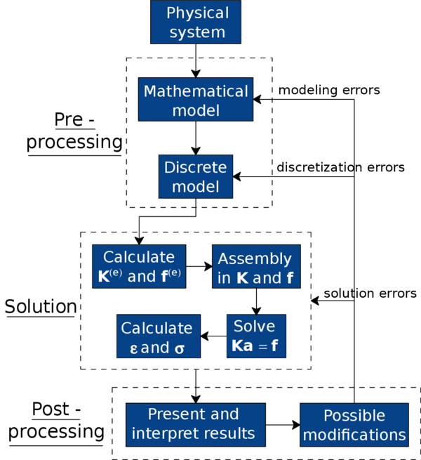
Figure 18: Global flowchart of the analysis of a system through the Finite Element Method.

Since the basis of the damage simulations performed in this work is a two-dimensional elastic finite element code, from now on we will be focusing on this kind of FEM problems.

3.2.1 Two-dimensional elasticity theory

A large variety of structures with a great interest for engineers can be studied with the hypothesis of two-dimensional elasticity. All these structures have in common an approximate right prism shape. Nonetheless, depending on the proportion of such prism dimensions and on the load configuration, the problems involving these structures can be classified in one of the following groups:

• Plane Stress Problems: one of the dimensions of the structure (thickness) is much smaller than the other two, and loads are contained in the mid-surface of that dimension (Figure 19).

• Plane Strain Problems: one of the dimensions of the structure (length) is much larger than the other two, and loads act uniformly distributed along this length, and are contained in planes orthogonal to the axis passing through the center of gravity of all cross sections (Figure 20).

Figure 19: Example of a plane stress problem.

Figure 20: Example of a plane strain problem.

3.2.1.1 Displacements, strains and stresses fields

In two-dimensional elasticity theory, a series of hypothesis are used in order to simplify the expressions defining displacements, strains and stresses. In the following lines we will be reviewing them.

The geometrical characteristics and load properties of a structure working in a plane state (plane stress or plane strain) permits stating the hypothesis that all sections perpendicular to the ${\textstyle z}$ axis suffer identical deformations contained in its own plane. This way, considering a generic cross section contained in the ${\textstyle x-y}$ plane of any of the structures in Figures 19 and 20, the displacement field of the structure can be perfectly defined if we know the displacement in the directions ${\textstyle x}$ and ${\textstyle y}$ for all points of that section. Thereby, the vector of displacements at any point is defined as:

${\boldsymbol {u}}(x,y)=\left\{{\begin{array}{c}u(x,y)\\v(x,y)\end{array}}\right\}$

(65)

where ${\textstyle u(x,y)}$ and ${\textstyle v(x,y)}$ are the displacements of the point in the directions ${\textstyle x}$ and ${\textstyle y}$, respectively.

From the displacements field (65) one can easily obtain the strains field following the general elasticity theory [51]:

$\varepsilon _{x}$ $=\displaystyle {\frac {\partial u}{\partial x}}$ $\varepsilon _{y}$ $=\displaystyle {\frac {\partial v}{\partial y}}$ (66) $\gamma _{xy}$ $=\displaystyle {\frac {\partial u}{\partial y}}+{\frac {\partial v}{\partial x}}$ $\gamma _{xz}$ $=\gamma _{yz}=0$

In plane strain problems, there is the additional hypothesis that the strain ${\textstyle \varepsilon _{z}}$ is null, whereas in plane stress problems it is the stress ${\textstyle \sigma _{z}}$ that is zero. This makes that, in any case, it is no necessary to consider strain ${\textstyle \varepsilon _{z}}$ because it does not take part in the work of deformations since ${\textstyle \sigma _{z}\varepsilon _{z}=0}$. Thereby, at any point in a plane stress or plane strain state, we can define the vector of significant strains like:

${\boldsymbol {\varepsilon }}=[\varepsilon _{x},\varepsilon _{y},\gamma _{xy}]^{T}$

(67)

From equations in (66) we can deduce that tangential stresses ${\textstyle \tau _{xz}}$ and ${\textstyle \tau _{yz}}$ are zero. Moreover, for the same reasons of the previous paragraph, stress ${\textstyle \sigma _{z}}$ does not work, and so the significant stress vector can be defined as follows:

${\boldsymbol {\sigma }}=[\sigma _{x},\sigma _{y},\tau _{xy}]^{T}$

(68)

Once the strains and stresses have been presented, it is important to stablish the relation between them. This relation can be deduced by applying the previously stated hypothesis into the three-dimensional constitutive equation of elasticity [51]. The elastic stress-strain relation can be written like:

${\boldsymbol {\sigma }}={\boldsymbol {E}}{\boldsymbol {\varepsilon }}$

(69)

where ${\textstyle {\boldsymbol {E}}}$ is the elastic constitutive matrix:

${\boldsymbol {E}}={\begin{bmatrix}E_{11}&E_{12}&0\\E_{21}&E_{22}&0\\0&0&E_{33}\end{bmatrix}}$

(70)

For elastic isotropic materials the values in matrix ${\textstyle {\boldsymbol {E}}}$ are given by:

${\hbox{Plane Stress }}$ $\qquad$ ${\hbox{Plane Strain }}$ $E_{11}=E_{22}={\frac {E}{1-\nu ^{2}}}$ $E_{11}=E_{22}={\frac {E(1-\nu )}{(1+\nu )(1-2\nu )}}$ $E_{12}=E_{21}=E_{11}\nu$ $E_{12}=E_{21}=E_{11}{\frac {\nu }{1-\nu }}$ (71) $E_{33}={\frac {E}{2(1+\nu )}}=G$ $E_{33}={\frac {E}{2(1+\nu )}}=G$

with ${\textstyle E}$ being the Young's modulus, and ${\textstyle \nu }$ the Poisson's ratio.

3.2.1.2 Natural coordinates and shape functions

One of the most important concepts of the Finite Element Method are the so called, shape functions. These functions ${\textstyle N}$ are defined at each node of a finite element and allow us to obtain the value of a nodal variable at any point of the element through interpolation.

We will present the expressions of the shape functions for the quadrilateral element of four nodes, and for the triangular element of three nodes, since these are the elements that have been used in this work. To do so, we will first introduce the concept of natural coordinates, that will be used in the expressions of the shape functions.

The natural coordinates ${\textstyle (\xi ,\eta )}$ are normalized coordinates, meaning that they range from -1 to +1, like it is shown in Figure 21. From this same figure it can be deduced that:

$\xi ={\frac {x-x_{c}}{a}}\qquad ;\qquad \eta ={\frac {y-y_{c}}{b}}$

(72)

where ${\textstyle x_{c}}$ and ${\textstyle y_{c}}$ are the coordinates of the center of the element. Moreover:

${\frac {d\xi }{dx}}={\frac {1}{a}}\qquad ;\qquad {\frac {d\eta }{dy}}={\frac {1}{b}}$

(73)

and so a differential of area is obtained like:

$dxdy=abd\xi d\eta$

(74)

and, as it will appear later on, the integral of a function ${\textstyle f(x,y)}$ over a rectangular element can be perform by means of the following transformation to the natural coordinates:

$\iint _{A^{(e)}}f(x,y)dxdy=\int _{-1}^{+1}\int _{-1}^{+1}g(\xi ,\eta )abd\xi d\eta$

(75)

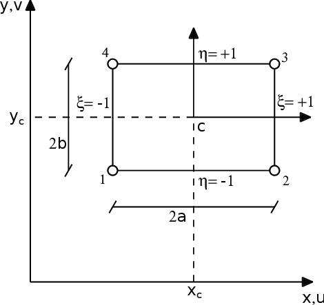
Figure 21: Geometry of a generic rectangular element. Natural and Cartesian coordinates.

In order to properly understand the expressions of the shape functions, it is interesting to introduce the complete polynomials in two-dimensions.

The shape functions can reproduce with no error polynomial variations of order less than or equal to the order of the complete polynomial contained in those shape functions. It can be deduced then, that the higher is the order of that complete polynomial, the more accurate can be the finite element solution.

In a 2D natural coordinates system, a complete polynomial of order ${\textstyle n}$ can be written like:

$f(\xi ,\eta )=\sum _{i=1}^{p}\alpha _{i}\xi ^{j}\eta ^{k}\qquad ;\qquad j+k\leq n$

(76)

where the number of terms of the polynomial is:

$p={\frac {(n+1)(n+2)}{2}}$

(77)

This way, a complete linear polynomial (${\textstyle n=1\rightarrow p=3}$) would be:

$f(\xi ,\eta )=\alpha _{1}+\alpha _{2}\xi {+\alpha }_{3}\eta$

(78)

An easy way to identify the terms of a 2D complete polynomial is by using the Pascal's triangle (Figure 22).

Figure 22: Pascal's triangle in two dimensions.

The shape functions of many elements (e.g. the 4-node quadrilateral) have terms of incomplete polynomials. Those terms generate nodal variables that barely contribute to the improvement of the element accuracy. Therefore, between two elements with shape functions containing complete polynomials of the same order, it is advisable to use that with less nodal variables.

That aside, all shape functions of an element must satisfy the following two conditions:

• Nodal compatibility condition

$N_{i}(\xi _{j},\eta _{j})=\left\{{\begin{array}{l}1\quad {\hbox{if }}i=j{\hbox{ }}\\0\quad {\hbox{if }}i\neq j{\hbox{ }}\end{array}}\right.\quad {\hbox{for }}\quad i,j=\{1,2,\dots ,n\}$

(79)

• Rigid body condition

$\sum _{i=1}^{n}N_{i}(\xi ,\eta )=1$

(80)

where ${\textstyle i}$ and ${\textstyle j}$ represent node indexes, and ${\textstyle n}$ is the number of nodes of the finite element.

At this point, we can already present the expressions of the shape functions, starting with the rectangular Lagrangian element of four nodes.

The shape functions of this element are based on polynomial interpolations of Lagrange in two dimensions. This permits defining the shape function of a generic node like the product between two uni-dimensional Lagrange polynomials in each direction of the two natural coordinates ${\textstyle \xi }$ and ${\textstyle \eta }$ at that node. Thereby, if we consider ${\textstyle l_{I}^{i}(\xi )}$ like the Lagrange polynomial of order ${\textstyle I}$ in direction ${\textstyle \xi }$ at node ${\textstyle i}$, and ${\textstyle l_{J}^{i}(\eta )}$ the one of order ${\textstyle J}$ in direction ${\textstyle \eta }$, the shape function at that node is:

$N_{i}(\xi ,\eta )=l_{I}^{i}(\xi )l_{J}^{i}(\eta )$

(81)

In particular, for the 4-node rectangular Lagrangian element, the uni-dimensional Lagrange polynomials in each direction ${\textstyle \xi }$ and ${\textstyle \eta }$ coincide with the shape functions of the 2-node bar element. Thereby, at a node ${\textstyle i}$ of the element we have:

$l_{1}^{i}(\xi )={\frac {1}{2}}(1+\xi \xi _{i})\qquad ;\qquad l_{1}^{i}(\eta )={\frac {1}{2}}(1+\eta \eta _{i})$

(82)

And consequently, the shape function at node ${\textstyle i}$ results:

$N_{i}(\xi ,\eta )=l_{1}^{i}(\xi )l_{1}^{i}(\eta )={\frac {1}{4}}(1+\xi \xi _{i})(1+\eta \eta _{i})$

(83)

The values of ${\textstyle \xi _{i}}$ and ${\textstyle \eta _{i}}$ can be seen in Figure 21 but are summarized in Table 4.

Table. 4 Natural coordinates for the rectangular Lagrangian element of four nodes.

Node	$\xi _{i}$	$\eta _{i}$
1	-1	-1
2	1	-1
3	1	1
4	-1	1

With regard to the triangular element of three nodes, we will present its shape functions also in terms of the natural coordinates, since it is how they are used in KRATOS.

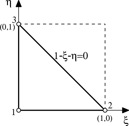
If we define a natural coordinates system over the normalized geometry of a triangular element, like in Figure 23, we can formulate the shape functions for each of its three nodes like:

$N_{1}=1-\xi {-\eta }\quad ;\quad N_{2}=\xi \quad ;\quad N_{3}=\eta$

(84)

Figure 23: Natural coordinates in a triangular element.

In this form, the triangular formulation becomes very similar to the quadrilateral one since, as it can be seen from figures 21 and 23, the normalized triangle is like a portion of a normalized square, which is very interesting when defining isoparametric elements.

3.2.1.3 Discretization of the displacements, strains and stresses fields

In summary, we have seen that thanks to the shape functions, one can obtain a variable at any point of the geometry through an interpolation from a limited number of nodal results.

Therefore, for a generic two-dimensional element of ${\textstyle n}$ nodes, we can write the displacement field like:

$u=\displaystyle \sum _{i=1}^{n}N_{i}u_{i}\quad ;\quad v=\displaystyle \sum _{i=1}^{n}N_{i}v_{i}$

(85)

where ${\textstyle (u_{i},v_{i})}$ and ${\textstyle N_{i}}$ are the horizontal and vertical displacements and the shape function of node ${\textstyle i}$. Equations in (85) can be rewritten in matrix format like:

${\boldsymbol {u}}={\begin{Bmatrix}u\\v\end{Bmatrix}}={\begin{bmatrix}N_{1}&0&\dots &N_{n}&0\\0&N_{1}&\dots &0&N_{n}\end{bmatrix}}{\begin{Bmatrix}u_{1}\\v_{1}\\\vdots \\u_{n}\\v_{n}\end{Bmatrix}}$

(86)

or equivalently:

${\boldsymbol {u}}={\boldsymbol {N}}{\boldsymbol {a}}^{(e)}$

(87)

where ${\textstyle {\boldsymbol {u}}}$ is the vector of displacements at a point of the element,

${\boldsymbol {N}}=[{\boldsymbol {N}}_{1},{\boldsymbol {N}}_{2},\dots ,{\boldsymbol {N}}_{n}]\qquad ;\qquad {\boldsymbol {N}}_{i}={\begin{bmatrix}N_{i}&0\\0&N_{i}\end{bmatrix}}$

(88)

are the matrix of shape functions of the element, and the matrix of shape functions of node ${\textstyle i}$, respectively, and

${\boldsymbol {a}}^{(e)}={\begin{Bmatrix}{\boldsymbol {a}}_{1}^{(e)}\\{\boldsymbol {a}}_{2}^{(e)}\\\vdots \\{\boldsymbol {a}}_{n}^{(e)}\end{Bmatrix}}\qquad ;\qquad {\boldsymbol {a}}_{i}^{(e)}={\begin{Bmatrix}u_{i}\\v_{i}\end{Bmatrix}}$

(89)

are the vector of nodal displacements of the element, and the vector of nodal displacements of node ${\textstyle i}$.

In the case of the strain field, we can write:

$\varepsilon _{x}$ $={\frac {\partial u}{\partial x}}=\sum _{i=1}^{n}{\frac {\partial N_{i}}{\partial x}}u_{i}$ $\varepsilon _{y}$ $={\frac {\partial v}{\partial y}}=\sum _{i=1}^{n}{\frac {\partial N_{i}}{\partial y}}v_{i}$ (90) $\gamma _{xy}$ $={\frac {\partial u}{\partial y}}+{\frac {\partial v}{\partial x}}=\sum _{i=1}^{n}\left({\frac {\partial N_{i}}{\partial y}}u_{i}+{\frac {\partial N_{i}}{\partial x}}v_{i}\right)$

and in matrix format:

${\boldsymbol {\varepsilon }}={\begin{Bmatrix}{\frac {\partial u}{\partial x}}\\{\frac {\partial v}{\partial y}}\\{\frac {\partial u}{\partial y}}+{\frac {\partial v}{\partial x}}\end{Bmatrix}}={\begin{bmatrix}{\frac {\partial N_{1}}{\partial x}}&0&\dots &{\frac {\partial N_{n}}{\partial x}}&0\\0&{\frac {\partial N_{1}}{\partial y}}&\dots &0&{\frac {\partial N_{n}}{\partial y}}\\{\frac {\partial N_{1}}{\partial y}}&{\frac {\partial N_{1}}{\partial x}}&\dots &{\frac {\partial N_{n}}{\partial y}}&{\frac {\partial N_{n}}{\partial x}}\end{bmatrix}}{\begin{Bmatrix}u_{1}\\v_{1}\\\vdots \\u_{n}\\v_{n}\end{Bmatrix}}$

(91)

or

${\boldsymbol {\varepsilon }}={\boldsymbol {B}}{\boldsymbol {a}}^{(e)}$

(92)

where

${\boldsymbol {B}}=[{\boldsymbol {B}}_{1},{\boldsymbol {B}}_{2},\dots ,{\boldsymbol {B}}_{n}]$

(93)

is the deformation matrix of the element, and

${\boldsymbol {B}}_{i}={\begin{bmatrix}\displaystyle {\frac {\partial N_{i}}{\partial x}}&0\\0&\displaystyle {\frac {\partial N_{i}}{\partial y}}\\\displaystyle {\frac {\partial N_{i}}{\partial y}}&\displaystyle {\frac {\partial N_{i}}{\partial x}}\end{bmatrix}}$

(94)

is the deformation matrix of node ${\textstyle i}$.

Now, substituting equation (92) in the relation (69), we can express the stress vector like:

${\boldsymbol {\sigma }}={\boldsymbol {E}}{\boldsymbol {\varepsilon }}={\boldsymbol {E}}{\boldsymbol {B}}{\boldsymbol {a}}^{(e)}$

(95)

If there were initial strains or stresses, they could be taken into account by using the following expression:

${\boldsymbol {\sigma }}={\boldsymbol {E}}({\boldsymbol {\varepsilon }}-{\boldsymbol {\varepsilon }}^{0})+{\boldsymbol {\sigma }}^{0}={\boldsymbol {E}}{\boldsymbol {B}}{\boldsymbol {a}}^{(e)}-{\boldsymbol {E}}{\boldsymbol {\varepsilon }}^{0}+{\boldsymbol {\sigma }}^{0}$

(96)

3.2.1.4 Equilibrium equations of the discretization

The expressions of the stiffness matrix ${\textstyle {\boldsymbol {K}}}$ and the force vector ${\textstyle {\boldsymbol {f}}}$ can be obtained form of the equilibrium equations of the discretization. To do so, we are going to start from the expression of the Principle of Virtual Works applied at the equilibrium of an element.

Let us suppose that uniformly distributed forces per unit area act over the body of the element (mass forces ${\textstyle {\boldsymbol {b}}}$), and uniformly distributed forces per unit length act over one of its sides (surface forces ${\textstyle {\boldsymbol {t}}}$). Moreover, supposing that the equilibrium of the element is achieved at the nodes, we define punctual forces acting at the nodes (nodal forces of equilibrium ${\textstyle {\boldsymbol {q}}}$) that must balance the forces that appear due to the element deformation as well as the rest of acting forces.

Thereby, we can write the Principle of Virtual Works applied at the element like:

$\iint _{A^{(e)}}\delta {\boldsymbol {\varepsilon }}^{T}{\boldsymbol {\sigma }}\;tdA=\iint _{A^{(e)}}\delta {\boldsymbol {u}}^{T}{\boldsymbol {b}}\;tdA+\oint _{l^{(e)}}\delta {\boldsymbol {u}}^{T}{\boldsymbol {t}}\;tds+[\delta {\boldsymbol {a}}^{(e)}]^{T}{\boldsymbol {q}}^{(e)}$

(97)

The first term of the expression represents the work of the stresses over the virtual strains ${\textstyle \delta {\boldsymbol {\varepsilon }}}$, whereas the terms on the right represent the work of the mass forces ${\textstyle {\boldsymbol {b}}}$, the surface forces ${\textstyle {\boldsymbol {t}}}$ and the punctual forces ${\textstyle {\boldsymbol {q}}^{(e)}}$ over the virtual displacements ${\textstyle \delta {\boldsymbol {u}}}$ and ${\textstyle \delta {\boldsymbol {a}}^{(e)}}$. ${\textstyle A^{(e)}}$ and ${\textstyle l^{(e)}}$ are the area and the contour of the element, and ${\textstyle t}$ is the thickness. In plane stress problems, ${\textstyle t}$ is the real thickness of the structure, while in plane strain ${\textstyle t}$ is usually taken as 1.

From (87) and (92), we can write:

$\delta {\boldsymbol {u}}^{T}=[\delta {\boldsymbol {a}}^{(e)}]^{T}{\boldsymbol {N}}^{T}\quad ;\quad \delta {\boldsymbol {\varepsilon }}^{T}=[\delta {\boldsymbol {a}}^{(e)}]^{T}{\boldsymbol {B}}^{T}$

(98)

Substituting (98) in (97), and rearranging terms, we obtain:

$[\delta {\boldsymbol {a}}^{(e)}]^{T}\left[\iint _{A^{(e)}}{\boldsymbol {B}}^{T}{\boldsymbol {\sigma }}\;tdA-\iint _{A^{(e)}}{\boldsymbol {N}}^{T}{\boldsymbol {b}}\;tdA-\oint _{l^{(e)}}{\boldsymbol {N}}^{T}{\boldsymbol {t}}\;tds\right]=[\delta {\boldsymbol {a}}^{(e)}]^{T}{\boldsymbol {q}}^{(e)}$

(99)

Since the virtual displacements ${\textstyle \delta {\boldsymbol {a}}^{(e)}}$ are arbitrary, we can write:

$\iint _{A^{(e)}}{\boldsymbol {B}}^{T}{\boldsymbol {\sigma }}\;tdA-\iint _{A^{(e)}}{\boldsymbol {N}}^{T}{\boldsymbol {b}}\;tdA-\oint _{l^{(e)}}{\boldsymbol {N}}^{T}{\boldsymbol {t}}\;tds={\boldsymbol {q}}^{(e)}$

(100)

Equation (100) represents the equilibrium between the nodal forces of equilibrium ${\textstyle {\boldsymbol {q}}^{(e)}}$ and the forces from the deformation of the element (first integral), the mass forces ${\textstyle {\boldsymbol {b}}}$ and the surface forces ${\textstyle {\boldsymbol {t}}}$. If we now substitute the stresses from expression (96), we get:

$\iint _{A^{(e)}}{\boldsymbol {B}}^{T}({\boldsymbol {E}}{\boldsymbol {B}}{\boldsymbol {a}}^{(e)}-{\boldsymbol {E}}{\boldsymbol {\varepsilon }}^{0}+{\boldsymbol {\sigma }}^{0})\;tdA-\iint _{A^{(e)}}{\boldsymbol {N}}^{T}{\boldsymbol {b}}\;tdA-\oint _{l^{(e)}}{\boldsymbol {N}}^{T}{\boldsymbol {t}}\;tds={\boldsymbol {q}}^{(e)}$

(101)

and rearranging terms:

$\left[\iint _{A^{(e)}}{\boldsymbol {B}}^{T}{\boldsymbol {E}}{\boldsymbol {B}}\;tdA\right]{\boldsymbol {a}}^{(e)}-\iint _{A^{(e)}}{\boldsymbol {B}}^{T}{\boldsymbol {E}}{\boldsymbol {\varepsilon }}^{0}\;tdA+$ $+\iint _{A^{(e)}}{\boldsymbol {B}}^{T}{\boldsymbol {\sigma }}^{0}\;tdA-\iint _{A^{(e)}}{\boldsymbol {N}}^{T}{\boldsymbol {b}}\;tdA-\oint _{l^{(e)}}{\boldsymbol {N}}^{T}{\boldsymbol {t}}\;tds={\boldsymbol {q}}^{(e)}$

(102)

which can be expressed like:

${\boldsymbol {K}}^{(e)}{\boldsymbol {a}}^{(e)}-{\boldsymbol {f}}^{(e)}={\boldsymbol {q}}^{(e)}$

(103)

where:

${\boldsymbol {K}}^{(e)}=\iint _{A^{(e)}}{\boldsymbol {B}}^{T}{\boldsymbol {E}}{\boldsymbol {B}}\;tdA$

(104)

is the elastic stiffness matrix of the element, and:

${\boldsymbol {f}}^{(e)}={\boldsymbol {f}}_{\varepsilon }^{(e)}+{\boldsymbol {f}}_{\sigma }^{(e)}+{\boldsymbol {f}}_{b}^{(e)}+{\boldsymbol {f}}_{t}^{(e)}$

(105)

is the vector of equivalent nodal forces of the element, with:

${\boldsymbol {f}}_{\varepsilon }^{(e)}=\iint _{A^{(e)}}{\boldsymbol {B}}^{T}{\boldsymbol {E}}{\boldsymbol {\varepsilon }}^{0}\;tdA\quad ;\quad {\boldsymbol {f}}_{\sigma }^{(e)}=-\iint _{A^{(e)}}{\boldsymbol {B}}^{T}{\boldsymbol {\sigma }}^{0}\;tdA$

(106)

being the vectors of equivalent nodal forces due to initial deformations and initial stresses, respectively;

${\boldsymbol {f}}_{b}^{(e)}=\iint _{A^{(e)}}{\boldsymbol {N}}^{T}{\boldsymbol {b}}\;tdA$

(107)

is the vector of equivalent nodal forces due to uniformly distributed forces per unit area; and

${\boldsymbol {f}}_{t}^{(e)}=\oint _{l^{(e)}}{\boldsymbol {N}}^{T}{\boldsymbol {t}}\;tds$

(108)

is the vector of equivalent nodal forces due to uniformly distributed forces per unit length.

The global equilibrium equation of the mesh is obtained by imposing that the sum of nodal forces of equilibrium at each node must equal the external nodal force:

$\sum _{e}{\boldsymbol {q}}_{i}^{(e)}={\boldsymbol {p}}_{j}$

(109)

where the left part of the expression represents the sum of contributions of the vectors of nodal forces of equilibrium of the different elements that share the global node ${\textstyle j}$, and ${\textstyle {\boldsymbol {p}}_{j}}$ represents the vector of external punctual forces acting on such node.

Therefore, the global equilibrium equation of the mesh can be obtained by assembling the contributions of stiffness matrices and vectors of equivalent nodal forces of the different elements. The global matrix equation can be written like:

${\boldsymbol {K}}{\boldsymbol {a}}={\boldsymbol {f}}$

(110)

where ${\textstyle {\boldsymbol {K}}}$, ${\textstyle {\boldsymbol {a}}}$ and ${\textstyle {\boldsymbol {f}}}$ are, respectively, the stiffness matrix, the vector of nodal displacements, and the vector of equivalent nodal forces of the whole mesh.

3.2.1.5 Isoparametric elements and numerical integration

At this point, we have already obtained the equilibrium equations of the discretization, but we have not presented yet a convenient numerical technique to integrate the expressions of the stiffness matrix and the vectors of equivalent nodal forces of the elements.

The integration of the expressions of the stiffness matrix and the vectors of equivalent nodal forces, will be performed by means of Gauss-Legendre quadratures. This technique allow us to integrate any function over a normalized domain, using tabulated Gauss point coordinates and weights. However, we need to transform first the integrals over the element domain into integrals over the normalized space of the natural coordinates.

In order to do so, we must first introduce a very important concept in the Finite Element Method: the isoparametric interpolation. In this regard, we will present the isoparametric quadrilateral elements, and the isoparametric triangular elements.

The concept of isoparametric interpolation comes from the usage of the same shape functions to interpolate the geometry and the displacements. Thereby, just as we saw in (85), we can express the geometry of a two-dimensional isoparametric element from the coordinates ${\textstyle x_{i}}$ and ${\textstyle y_{i}}$ of its nodes like:

$x=\sum _{i=1}^{n}N_{i}(\xi ,\eta )x_{i}\quad ;\quad y=\sum _{i=1}^{n}N_{i}(\xi ,\eta )y_{i}$

(111)

where ${\textstyle N_{i}(\xi ,\eta )}$ are the element shape functions. Equations in (111) relate the cartesian coordinates of a point with the natural coordinates ${\textstyle \xi }$ and ${\textstyle \eta }$, which is very convenient for the transformation of the integration domain.

In this regard, in order to formulate the change of variables from cartesian coordinates to natural coordinates, we need to compute the determinant of the Jacobian matrix. This can be obtained by deriving the shape functions with respect to ${\textstyle \xi }$ and ${\textstyle \eta }$. If we consider ${\textstyle N_{i}(\xi ,\eta )=N_{i}(x(\xi ,\eta ),y(\xi ,\eta ))}$ then, applying the chain rule, we have:

${\begin{array}{l}\displaystyle {\frac {\partial N_{i}}{\partial \xi }}=\displaystyle {\frac {\partial N_{i}}{\partial x}}{\frac {\partial x}{\partial \xi }}+{\frac {\partial N_{i}}{\partial y}}{\frac {\partial y}{\partial \xi }}\\\\\displaystyle {\frac {\partial N_{i}}{\partial \eta }}=\displaystyle {\frac {\partial N_{i}}{\partial x}}{\frac {\partial x}{\partial \eta }}+{\frac {\partial N_{i}}{\partial y}}{\frac {\partial y}{\partial \eta }}\end{array}}$

(112)

or in matrix format:

${\begin{Bmatrix}{\frac {\partial N_{i}}{\partial \xi }}\\{\frac {\partial N_{i}}{\partial \eta }}\end{Bmatrix}}={\begin{bmatrix}{\frac {\partial x}{\partial \xi }}&{\frac {\partial y}{\partial \xi }}\\{\frac {\partial x}{\partial \eta }}&{\frac {\partial y}{\partial \eta }}\end{bmatrix}}{\begin{Bmatrix}{\frac {\partial N_{i}}{\partial x}}\\{\frac {\partial N_{i}}{\partial y}}\end{Bmatrix}}={\boldsymbol {J}}^{(e)}{\begin{Bmatrix}{\frac {\partial N_{i}}{\partial x}}\\{\frac {\partial N_{i}}{\partial y}}\end{Bmatrix}}$

(113)

where ${\textstyle {\boldsymbol {J}}^{(e)}}$ is the Jacobian matrix of the transformation of natural coordinates to cartesian coordinates. From (113) we can derive:

${\begin{Bmatrix}{\frac {\partial N_{i}}{\partial x}}\\{\frac {\partial N_{i}}{\partial y}}\end{Bmatrix}}=\left[{\boldsymbol {J^{(e)}}}\right]^{-1}{\begin{Bmatrix}{\frac {\partial N_{i}}{\partial \xi }}\\{\frac {\partial N_{i}}{\partial \eta }}\end{Bmatrix}}={\frac {1}{\left|{\boldsymbol {J}}^{(e)}\right|}}{\begin{bmatrix}{\frac {\partial y}{\partial \eta }}&-{\frac {\partial y}{\partial \xi }}\\-{\frac {\partial x}{\partial \eta }}&{\frac {\partial x}{\partial \xi }}\end{bmatrix}}{\begin{Bmatrix}{\frac {\partial N_{i}}{\partial \xi }}\\{\frac {\partial N_{i}}{\partial \eta }}\end{Bmatrix}}$

(114)

where ${\textstyle \left|{\boldsymbol {J}}^{(e)}\right|}$ is the determinant of the Jacobian.

The determinant of the Jacobian permits expressing the differential of area in natural coordinates [52] like:

$dx\;dy=\left|{\boldsymbol {J}}^{(e)}\right|d\xi \;d\eta$

(115)

Now, using the isoparametric transformation (111) we can obtain the terms of the Jacobian:

${\frac {\partial x}{\partial \xi }}=\sum _{i=1}^{n}{\frac {\partial N_{i}}{\partial \xi }}x_{i}\quad ;\quad {\frac {\partial x}{\partial \eta }}=\sum _{i=1}^{n}{\frac {\partial N_{i}}{\partial \eta }}x_{i}\quad ;\quad {\hbox{etc. }}$

and so:

${\boldsymbol {J}}^{(e)}=\sum _{i=1}^{n}{\begin{bmatrix}{\frac {\partial N_{i}}{\partial \xi }}x_{i}&{\frac {\partial N_{i}}{\partial \xi }}y_{i}\\{\frac {\partial N_{i}}{\partial \eta }}x_{i}&{\frac {\partial N_{i}}{\partial \eta }}y_{i}\end{bmatrix}}$

(116)

Furthermore, substituting the expressions of equation (114) in (94) we obtain the deformation matrix of an isoparametric element in terms of the natural coordinates:

${\boldsymbol {B}}_{i}(\xi ,\eta )={\frac {1}{\left|{\boldsymbol {J}}^{(e)}\right|}}{\begin{bmatrix}b_{i}&0\\0&c_{i}\\c_{i}&b_{i}\end{bmatrix}}$

(117)

where

$b_{i}={\frac {\partial y}{\partial \eta }}{\frac {N_{i}}{\partial \xi }}-{\frac {\partial y}{\partial \xi }}{\frac {\partial N_{i}}{\partial \eta }}\quad ;\quad c_{i}={\frac {\partial x}{\partial \xi }}{\frac {N_{i}}{\partial \eta }}-{\frac {\partial x}{\partial \eta }}{\frac {\partial N_{i}}{\partial \xi }}$

(118)

Finally, by applying the previous expressions, the elastic stiffness matrix (104) can be written like an integral over the normalized domain of the natural coordinates.

For quadrilateral elements we have:

${\boldsymbol {K}}^{(e)}=\iint _{A^{(e)}}{\boldsymbol {B}}^{T}{\boldsymbol {E}}{\boldsymbol {B}}\;tdxdy=\int _{-1}^{+1}\int _{-1}^{+1}{\boldsymbol {B}}^{T}(\xi ,\eta ){\boldsymbol {E}}{\boldsymbol {B}}(\xi ,\eta )\left|{\boldsymbol {J}}^{(e)}\right|\;td\xi d\eta$

(119)

And for triangular elements we must consider the different domain of integration (see Figure 23):

${\boldsymbol {K}}^{(e)}=\int _{0}^{1}\int _{0}^{1-\eta }{\boldsymbol {B}}^{T}(\xi ,\eta ){\boldsymbol {E}}{\boldsymbol {B}}(\xi ,\eta )\left|{\boldsymbol {J}}^{(e)}\right|\;td\xi d\eta$

(120)

At this point we can already use the Gauss quadrature to solve the integrals of the previous expressions. First, though, let us remind the fundamentals of the Gauss-Legendre quadrature for rectangular and triangular domains.

The integral of a generic function ${\textstyle g(\xi ,\eta )}$ over the domain of natural coordinates of a quadrilateral element can be evaluated by means of a Gauss quadrature like:

$\int _{-1}^{+1}\int _{-1}^{+1}g(\xi ,\eta )d\xi d\eta =\int _{-1}^{+1}d\xi \left[\sum _{q=1}^{n_{q}}g(\xi ,\eta _{q})W_{q}\right]=\sum _{p=1}^{n_{p}}\sum _{q=1}^{n_{q}}g(\xi _{p},\eta _{q})W_{p}W_{q}$

(121)

where ${\textstyle n_{p}}$ and ${\textstyle n_{q}}$ are the number of integration points in each direction ${\textstyle \xi }$ and ${\textstyle \eta }$; ${\textstyle \xi _{p}}$ and ${\textstyle \eta _{q}}$ are the natural coordinates of the integration points ${\textstyle p}$, ${\textstyle q}$ and ${\textstyle W_{p}}$, ${\textstyle W_{q}}$ the weights of that point corresponding to each direction.

On the other hand, the Gauss quadrature for a triangular element can be written like:

$\int _{0}^{1}\int _{0}^{1-\eta }g(\xi ,\eta )d\xi d\eta =\sum _{p=1}^{n_{p}}g(\xi _{p},\eta _{p})W_{p}$

(122)

The coordinates and weights of the integration points are tabulated. And the number of integration points must be properly chosen, taking into account that a Gauss quadrature of order ${\textstyle n}$ in each natural direction permits integrating with no error a polynomial of order ${\textstyle \leq 2n-1}$ in the corresponding natural coordinate. In our case, we have been using 2x2 integration points for the quadrilateral elements of four nodes, and 1 integration point for the triangular elements of three nodes.

Now, substituting (121) in (119), we can obtain the expression of the elastic stiffness matrix for an isoparametric quadrilateral element, evaluated through numerical integration:

${\boldsymbol {K}}^{(e)}=\int _{-1}^{+1}\int _{-1}^{+1}{\boldsymbol {B}}^{T}{\boldsymbol {E}}{\boldsymbol {B}}\left|{\boldsymbol {J}}^{(e)}\right|\;td\xi d\eta =\sum _{p=1}^{n_{p}}\sum _{q=1}^{n_{q}}\left[{\boldsymbol {B}}^{T}{\boldsymbol {E}}{\boldsymbol {B}}\left|{\boldsymbol {J}}^{(e)}\right|t\right]_{p,q}W_{p}W_{q}$

(123)

And from (120) and (122) we obtain the expression corresponding to a triangular element:

${\boldsymbol {K}}^{(e)}=\int _{0}^{1}\int _{0}^{1-\eta }{\boldsymbol {B}}^{T}{\boldsymbol {E}}{\boldsymbol {B}}\left|{\boldsymbol {J}}^{(e)}\right|\;td\xi d\eta =\sum _{p=1}^{n_{p}}\left[{\boldsymbol {B}}^{T}{\boldsymbol {E}}{\boldsymbol {B}}\left|{\boldsymbol {J}}^{(e)}\right|t\right]_{p}W_{p}$

(124)

Thereby, we can see that the numerical integration of the stiffness matrix requires the evaluation of the Jacobian ${\textstyle {\boldsymbol {J}}^{(e)}}$, its determinant ${\textstyle \left|{\boldsymbol {J}}^{(e)}\right|}$, the deformation matrix ${\textstyle {\boldsymbol {B}}}$, the constitutive matrix ${\textstyle {\boldsymbol {E}}}$, and the thickness ${\textstyle t}$ at each integration point.

Similarly, the computation of any of the vectors of equivalent nodal forces that imply integrals over a quadrilateral element, for instance (107), can be performed like:

${\boldsymbol {f}}_{b}^{(e)}$ $=\iint _{A^{(e)}}{\boldsymbol {N}}^{T}{\boldsymbol {b}}tdxdy=\int _{-1}^{+1}\int _{-1}^{+1}{\boldsymbol {N}}^{T}{\boldsymbol {b}}\left|{\boldsymbol {J}}^{(e)}\right|td\xi d\eta$ $=\sum _{p=1}^{n_{p}}\sum _{q=1}^{n_{q}}\left[{\boldsymbol {N}}^{T}{\boldsymbol {b}}\left|{\boldsymbol {J}}^{(e)}\right|t\right]_{p,q}W_{p}W_{q}$

(125)

For triangular elements the double sum is replaced by the simple sum of (122).

Finally, the computation of the vector of surface forces (108) is a bit different because the integral is performed over the contour of the element ${\textstyle l^{(e)}}$. In general, such contour represents a straight line ${\textstyle \xi =}$const or ${\textstyle \eta =}$const in the space of natural coordinates. Therefore, for example, for a contour of an isoparametric quadrilateral element corresponding to the straight line ${\textstyle \eta =1}$, the differential of length ${\textstyle ds}$ is computed like:

$[ds]_{\eta =1}$ $=\left[{\sqrt {dx^{2}+dy^{2}}}\right]_{\eta =1}=\left[{\sqrt {\left({\frac {dx}{d\xi }}\right)_{\eta =1}^{2}+\left({\frac {dy}{d\xi }}\right)_{\eta =1}^{2}}}\right]d\xi$ $=\left[{\sqrt {\left(\sum _{i=1}^{n}{\frac {dN_{i}}{d\xi }}x_{i}\right)_{\eta =1}^{2}+\left(\sum _{i=1}^{n}{\frac {dN_{i}}{d\xi }}y_{i}\right)_{\eta =1}^{2}}}\right]d\xi =c(\xi )d\xi$

(126)

Substituting (126) in (108) we obtain a line integral that depends only on the natural coordinate ${\textstyle \xi }$ and that can be computed through a uni-dimensional quadrature like:

${\boldsymbol {f}}_{t}^{(e)}=\oint _{l^{(e)}}\left[{\boldsymbol {N}}^{T}\right]_{\eta =1}{\boldsymbol {t}}\;t\;c(\xi )d\xi =\int _{-1}^{+1}{\boldsymbol {g}}(\xi )d\xi =\sum _{p=1}^{n_{p}}{\boldsymbol {g}}(\xi _{p})W_{p}$

(127)

A more extended overview on the Finite Element Method can be found in [53,54].

3.3 Non-linearity Associated to Damage

In the previous section we reviewed fundamental concepts on the Finite Element Method centering our attention on the two-dimensional elasticity theory, which is the basis of the implemented damage code.

In this regard, when deriving the equilibrium equations of the discretization from the Principle of Virtual Works (97), we used an elastic stress-strain relation (69). Nonetheless, in the previous chapter we explained that in order to take into account the lost of stiffness due to damage progression, a different stress-strain relation had to be used.

If we now consider the stress-strain law (13) in voigt notation:

${\boldsymbol {\sigma }}={\boldsymbol {E}}_{sec}{\boldsymbol {\varepsilon }}=(1-d){\boldsymbol {E}}{\boldsymbol {\varepsilon }}$

(128)

and we introduce it into a general expression of the PVW (100), we obtain the following relation:

$\left[\iint _{A^{(e)}}{\boldsymbol {B}}^{T}(1-d){\boldsymbol {E}}{\boldsymbol {B}}tdA\right]{\boldsymbol {a}}^{(e)}-\iint _{A^{(e)}}{\boldsymbol {N}}^{T}{\boldsymbol {b}}\;tdA-\oint _{l^{(e)}}{\boldsymbol {N}}^{T}{\boldsymbol {t}}\;tds={\boldsymbol {q}}^{(e)}$

(129)

where ${\textstyle d}$ is the damage parameter.

Expression (129) can be rewritten like:

${\boldsymbol {K}}^{(e)}(d)\,{\boldsymbol {a}}^{(e)}-{\boldsymbol {f}}^{(e)}={\boldsymbol {q}}^{(e)}$

(130)

where

${\boldsymbol {K}}^{(e)}(d)=\iint _{A^{(e)}}{\boldsymbol {B}}^{T}(1-d){\boldsymbol {E}}{\boldsymbol {B}}tdA$

(131)

is the damaged or secant stiffness matrix of the element, and

${\boldsymbol {f}}^{(e)}={\boldsymbol {f}}_{b}^{(e)}+{\boldsymbol {f}}_{t}^{(e)}$

(132)

is the vector of equivalent nodal forces of the element, in which ${\textstyle {\boldsymbol {f}}_{b}^{(e)}}$ and ${\textstyle {\boldsymbol {f}}_{t}^{(e)}}$ coincide with (107) and (108), respectively.

Like we stated before, by assembling the contributions of the different elements of the mesh we can obtain the global matrix equation:

${\boldsymbol {K}}(d)\,{\boldsymbol {a}}={\boldsymbol {f}}$

(133)

where ${\textstyle {\boldsymbol {K}}(d)}$ is the global secant stiffness matrix ${\textstyle {\boldsymbol {K}}_{sec}}$.

By the way, we saw in Chapter 2 that ${\textstyle d=g(r)}$, where ${\textstyle r}$ is the internal state variable depending on the equivalent strains ${\textstyle \varepsilon _{eq}}$. Therefore, since the strains are directly related to the displacements through (92), we can say that damage also depends on the displacements, i.e. ${\textstyle d=f({\boldsymbol {a}})}$. Taking into account this last consideration, expression (133) results:

${\boldsymbol {K}}_{sec}({\boldsymbol {a}})\,{\boldsymbol {a}}={\boldsymbol {f}}$

(134)

which is a non-linear system of equations.

Thereby, the inclusion of damage mechanics in the classical elasticity theory introduces a non-linearity that must be taken into account when solving this kind of problems. In this section we are going to review how we solve such non-linear system of equations, but before let us introduce the fundamentals of non-linear problems that will help us understand the results of the simulations performed.

3.3.1 Fundamentals of non-linear problems

Let us begin by introducing the term response as a pictorial characterization of non-linearity of a structural system. Response is a graphical representation of the fundamental concept of equilibrium path. Through this representation many concepts can be illustrated and interpreted in physical, mathematical or computational terms.

In this regard, a solid mechanics problem is said to be non-linear when the response diagram is not proportional, i.e. when it does not follow Hooke's law.

The most widely used form of these pictures is the load-deflection response diagram. Given an action parameter (e.g. the applied load) and a response parameter (e.g. the displacement), one can plot a response diagram for the equilibrium path of any system. In fact, real problems have multidimensional response diagrams but, in order to make it understandable, they are usually represented from two representative variables. Figure 24 shows two possible non-linear response diagrams.

Figure 24: Response diagrams: (a)Load-deflection diagram showing equilibrium path. (b)Diagram distinguishing primary from secondary equilibrium path.

3.3.1.1 Terminology

Before going into the different kinds of non-linear behaviour, let us briefly introduce some basic terminology concerning response diagrams.

The continuous curve shown in a load-deflection diagram is called a path. Paths are piecewise smooth, that is, they have a continuous tangent except at some exceptional points.

Each point in the path represents a possible configuration state of the structure. If the path represents configurations in static equilibrium it is called equilibrium path.

The origin of the response diagram (zero load and zero deflection) is called the reference state because it is the configuration from which loads and deflections are measured.

For ideal cases, the reference state is unstressed and undeformed, and it is also an equilibrium state. This means that an equilibrium path passes through the reference state like in Figure 24.a.

The path that crosses the reference state is called the fundamental equilibrium path, fundamental path or primary path. The fundamental path extends from the reference state up to special states called critical points. Any path that is not a fundamental path but connects with it at a critical point is called a secondary equilibrium path or secondary path (see Figure 24.b).

Qualifiers "primary" and "secondary" are linked with the relative importance of these equilibrium paths in design. Most structures are designed to operate in the fundamental path, with some sort of safety factor against reaching a critical point. However, knowledge of secondary paths may be important in some aspects of the design process, for example in the assessment of structural behaviour under emergency scenarios.

Apart from the stated terminology, there are a pair of additional concepts involving the response diagram that must be pointed out.

The tangent to an equilibrium path may be informally viewed as the limit of the ratio between a force increment and a displacement increment. This is by definition the tangent stiffness associated to the representative force-displacement diagram.

The sign of the tangent stiffness is closely related to the question of stability of an equilibrium state. A negative stiffness is necessarily associated to unstable equilibrium, whereas a positive stiffness is necessary but not sufficient for stability.

If the load and deflection quantities are conjugate in the virtual work sense, the area under a load-deflection diagram may be interpreted as work performed by the system or energy spent in the deformation process.

3.3.1.2 Special equilibrium points

As we have seen, certain points of an equilibrium path have special significance in the applications and thus receive special names. Of particular interest are critical, turning, and failure points.

Critical points can be classified in two groups: limit points, at which the tangent to the equilibrium path is horizontal; and bifurcation points, at which two or more equilibrium paths cross. At critical points the relation between the characteristic load and the associated deflection is not unique. At these points, the structure becomes physically uncontrollable, and so they have engineering significance from a design perspective.

Turning points are states at which the tangent to the equilibrium path is vertical. These are not critical points and have less physical significance, although they can be of interest in connection with the so-called "snap-back" phenomenon. However, turning points may have computational significance because they can affect the performance of certain "path following" solution methods.

Finally, points at which a path suddenly stops or breaks because of physical failure are called failure points. The phenomenon of failure may be local or global in nature. In the first case the structure may regain functional equilibrium after dynamically jumping to another equilibrium path. In the latter case the failure is catastrophic and so the structure cannot regain functional equilibrium.

3.3.1.3 Linear response

A few lines above, we stated that a system is considered non-linear when the response is not proportional. In order to properly understand what a non-linear problem implies, let us first present what a linear response is.

A linear system is a mathematical model characterized by a linear fundamental equilibrium path for all possible choices of load and deflection variables. The consequences of such behaviour are the following:

• A linear structure can sustain any load level and undergo any displacement magnitude.
• There are no critical, turning or failure points.
• Response to different load systems can be obtained by superposition.
• Removing all loads returns the structure to the reference position

The requirements for such a model to be applicable are:

• Perfect linear elasticity for any deformation
• Infinitesimal deformations
• Infinite strength

These assumptions are not only physically unrealistic but mutually contradictory, and thus there are necessarily limits placed on the validity of a linear model. Nevertheless, the linear model can be a good approximation of portions of the non-linear response, for instance, the fundamental path in the vicinity of the reference state. Thereby, since for many structures this segment represents the operational range, the linear model is widely used in design calculations.

3.3.1.4 Response behaviours

Once the linear regime is abandoned, the response diagram may present different basic types of behaviour. Let us present some interesting cases.

Figure 25 illustrates three monotonic types of response: linear, hardening, and softening. Symbols ${\textstyle R}$, ${\textstyle F}$ and ${\textstyle L}$ identify reference, failure and limit points, respectively.

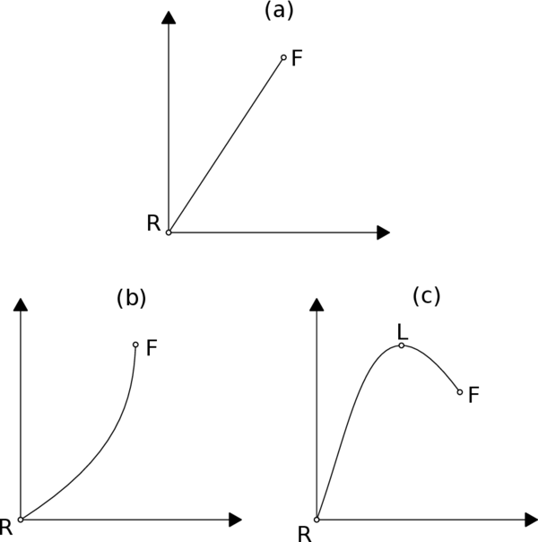
Figure 25: Basic behaviours for a non-linear response. (a)Linear until brittle failure. (b)Hardening. (c)Softening.

The response shown in Figure 25.a: linear until fracture, is characteristic of pure crystals, glassy, as well as certain high strength composite materials that contain such materials as fibers.

The response illustrated by Figure 25.b is typical of cable, netted and pneumatic (inflatable) structures. The stiffening effect comes from geometry adaptation to the applied loads.

A response such as in Figure 25.b is more common for structure materials, like concrete or steel, than the previous two. A linear branch is followed by a softening regime that may occur suddenly or gradually.

The diagrams of Figure 26 show a combination of basic behaviours that can complicate the response of the structure. Here ${\textstyle B}$ and ${\textstyle T}$ denote bifurcation and turning points.

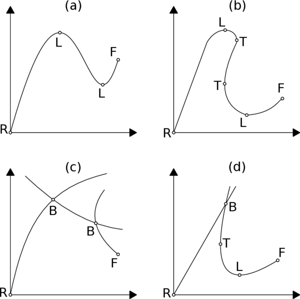
Figure 26: Complex non-linear responses. (a)Snap-through. (b)Snap-back. (c)Bifurcation. (d)Bifurcation with snap-back.

The snap-through response in Figure 26.a combines softening with hardening following the second limit point. The response branch between the two limit points has a negative stiffness and is therefore unstable. A response of this type is typical of slightly curved structures such as shallow arches.

The snap-back in Figure 26.b is an exaggerated snap-through, in which the response curve turns back in itself at the turning points. The equilibrium between the two turning points may be stable and physically realizable. This type of response is exhibited by folded and thin shell structures in which moving arch effects occur following the first limit point.

In the previous diagrams the response was a unique curve. Nevertheless, at bifurcation points of Figures 26.b and 26.c more than one response path is possible. The structure takes the path that is dynamically preferred over the others, i.e., the path that implies spending less energy. Bifurcation points can appear in any sufficient thin structure that experiences compressive stresses.

3.3.1.5 Sources of non-linearities

A response diagram characterizes only the gross behaviour of a structure, as it could be observed by performing an experiment on a mechanical testing machine. Further insight into the source of non-linearity is required to capture such physical behaviour with mathematical and computational models.

For structural analysis we can encounter four sources of non-linear behaviour: geometric, material, force boundary conditions, and displacement boundary conditions.

Geometric non-linearities appear when the difference between the deformed and undeformed configurations is taken into account when setting up the strain-displacement and equilibrium equations. Examples of geometric non-linearities include: slender structures in aerospace, civil and mechanical engineering applications; tensile structures such as cables and inflatable membranes; metal and plastic forming, etc.

Material non-linearity is the case of systems whose constitutive behaviour depends on the current deformation state and possibly past history of the deformation. Other constitutive variables may be involved. We can find material non-linearity in structures undergoing non-linear elasticity, plasticity, visco-elasticity, damage, creep, etc.

Non-linear force boundary conditions are applied forces that depend on the deformation. The most important engineering applications concerns pressure loads of fluids. These include hydrostatic loads on submerged or container structures; aerodynamic and hydrodynamic loads (wind loads, wave loads, drag forces). Also gyroscopic and non-conservative followers forces are of mathematical interest.

Lastly, displacement boundary conditions non-linearities come from displacement boundary conditions that depend on the deformation of the structure. The most well-known application is the contact problem, in which no-interpenetration conditions are enforced on flexible bodies while the extent of the contact area is unknown. Non-structural applications of this problem include: ice melting, phase changes, flow in porous media, etc.

Our damage mechanics problem falls into the material non-linearity category, and we will be working with conservative loads and constant boundary conditions.

3.3.2 Strategies for the solution of non-linear problems

After reviewing the different response behaviours of non-linearity as well as the sources behind it, one can clearly see that it is not easy to deal with non-linear problems. Several difficulties may arise due to a number of reasons.

The proper definition of the non-linear problem is one of these reasons. Indeed, most of the non-linear models are build "neglecting" many of the non-linear effects presents in the problem (coupling between various phenomena, geometric non-linearity, material non-linearities, contact, etc.).

Another difficulty comes from the lack of uniqueness. In non-linear problems existence and uniqueness of the solution is not guaranteed. Neither it is possible to estimate the computational cost of finding one or more solutions.

Besides, even when one finds a possible solution, the reliability of that solution depends on the robustness of the algorithm used. Usually, parametric studies are necessary to verify the solution (type and number of finite elements used, size of the time steps, boundary conditions, etc.). Furthermore, numerical problems appear when the original problem is not sufficiently well posed, that is, it is not correctly formulated.

Taking into account these difficulties, let us present one of the most widely used strategies to solve non-linear problems like the one in this work.

3.3.2.1 Incremental-iterative methods

Because of the lack of uniqueness of the solution, in many cases the correct solution is path dependent and so it depends on the path followed to reach a given equilibrium state.

In this regard, in many cases it is advisable to follow the physics of the problem and consider the solution, not only as the response to a given action, but as a full historical sequence of the successive states of equilibrium that go from the reference state to another one.

Apart from the stated above, it is interesting to follow the full history of a non-linear process because it gives more information on the mechanical behaviour of the system (engineering reason); and it also helps tracing the equilibrium path near critical points and facilitates convergence (mathematical reason).

Thereby, the method for solving non-linear solid mechanic problems consists on following the equilibrium path by using incrementation or continuity strategies. Assuming the action and the response is known at a given equilibrium state, a new equilibrium state is sought, located on the same branch of equilibrium path and a certain distance from the previous one.

Three different strategies for advance control are typically used:

1. Control of the action or force control: The action (force) is incremented and the corresponding incremental change in the response (displacement) is computed. This is the more commonly used method because of its simplicity, but it is unable to overcome limit points. (Figure 27.a)
2. Control of the response or displacement control: The response (displacement) is incremented and the corresponding incremental change in the action (force) is computed. It allows to overcome limit points, but it cannot deal with turning points. (Figure 27.b)
3. Mixed control or arc-length control: A nearby point on the equilibrium path is sought at a given distance from the previous equilibrium point, measured with a certain norm in the mixed space of action-response (load-displacement). This method is very general and allows overcoming limits and turning points, although its effectiveness depends on the selection of the appropriate distance norm. (Figure 27.c)

Figure 27 displays the geometric representation of the three strategies for advance control presented. In this figure, S represents the last solution point, P is the predicted point, and C is the converged solution after a corrective process.

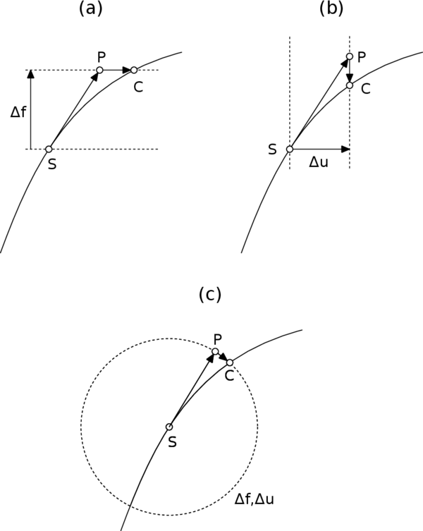
Figure 27: Geometric representations of different strategies for advance control: (a)Force control. (b)Displacement control. (c)Arc-length control

In order to clearly explain the incremental-iterative concept, let us formulate our case using the simple force control strategy as example.

The non-linear system of equations obtained in a damage mechanics problem (134) can be expressed like the residual between the internal and the external forces. Thereby, at step ${\textstyle n}$ of a force control strategy we can write:

${\boldsymbol {R}}(^{n}{\boldsymbol {a}})={\boldsymbol {f}}_{int}(^{n}{\boldsymbol {a}})-{^{n}{\boldsymbol {f}}}_{ext}={\boldsymbol {0}}$

(135)

where

${\boldsymbol {f}}_{int}(^{n}{\boldsymbol {a}})={\boldsymbol {K}}_{sec}(^{n}{\boldsymbol {a}})\,^{n}{\boldsymbol {a}}$

(136)

and ${\textstyle ^{n}{\boldsymbol {f}}_{ext}}$ is the vector of external forces at the load step ${\textstyle n}$, i.e. ${\textstyle ^{n}{\boldsymbol {f}}_{ext}\equiv {^{n}{\boldsymbol {f}}}}$.

Supposing that step ${\textstyle n}$ is in equilibrium, we must first increase the external load by a prescribed ${\textstyle {^{n+1}\Delta }{\boldsymbol {f}}_{ext}}$. Consequently, the new external force is:

$^{n+1}{\boldsymbol {f}}_{ext}={^{n}{\boldsymbol {f}}}_{ext}+{^{n+1}\Delta }{\boldsymbol {f}}_{ext}$

(137)

The unknown is the incremental displacement ${\textstyle ^{n+1}\Delta {\boldsymbol {a}}}$ that results from the previous force increment. Thereby:

$^{n+1}{\boldsymbol {a}}={^{n}{\boldsymbol {a}}}+{^{n+1}\Delta }{\boldsymbol {a}}$

(138)

Imposing equilibrium at the sought solution we obtain the equation that must be solved:

${\boldsymbol {0}}$ $={\boldsymbol {R}}(^{n+1}{\boldsymbol {a}})={\boldsymbol {f}}_{int}(^{n+1}{\boldsymbol {a}})-{^{n+1}{\boldsymbol {f}}}_{ext}$ $={\boldsymbol {f}}_{int}({^{n}{\boldsymbol {a}}}+{^{n+1}\Delta }{\boldsymbol {a}})-{^{n}{\boldsymbol {f}}}_{ext}-{^{n+1}\Delta }{\boldsymbol {f}}_{ext}$

(139)

There are many methods that can be applied to compute ${\textstyle ^{n+1}\Delta {\boldsymbol {a}}}$, but perhaps the most used are the secant matrix method and the tangent matrix method.

With the first method, the internal forces are described by the secant stiffness matrix at the previous equilibrium point:

${\boldsymbol {f}}_{int}({^{n}{\boldsymbol {a}}}+{^{n+1}\Delta }{\boldsymbol {a}})\approx {\boldsymbol {K}}_{sec}(^{n}{\boldsymbol {a}})({^{n}{\boldsymbol {a}}}+{^{n+1}\Delta }{\boldsymbol {a}})$

(140)

Then one just needs to solve the resulting linear system of equations:

${\boldsymbol {K}}_{sec}(^{n}{\boldsymbol {a}})({^{n}{\boldsymbol {a}}}+{^{n+1}\Delta }{\boldsymbol {a}})={^{n}{\boldsymbol {f}}}_{ext}+{^{n+1}\Delta }{\boldsymbol {f}}_{ext}$

(141)

or equivalently

${\boldsymbol {K}}_{sec}(^{n}{\boldsymbol {a}})\,={^{n+1}{\boldsymbol {f}}}_{ext}$

(142)

On the other hand, the tangent matrix method is based on a linearization of the problem. This means that the internal forces are represented through a Taylor series expanded to first order, neglecting the higher order terms:

${\boldsymbol {f}}_{int}({\boldsymbol {a}}+\Delta {\boldsymbol {a}})={\boldsymbol {f}}_{int}({\boldsymbol {a}})+{\frac {\partial {\boldsymbol {f}}_{int}}{\partial {\boldsymbol {a}}}}\Delta {\boldsymbol {a}}+\dots$

(143)

where the derivative of the internal forces with respect to the vector of nodal displacements is the global tangent stiffness matrix:

${\boldsymbol {K}}_{tan}={\frac {\partial {\boldsymbol {f}}_{int}}{\partial {\boldsymbol {a}}}}$

(144)

Substituting (143) in (139) we obtain:

${\boldsymbol {0}}={\boldsymbol {f}}_{int}(^{n}{\boldsymbol {a}})+{\boldsymbol {K}}_{tan}(^{n}{\boldsymbol {a}})\,{\boldsymbol {a}}-{^{n}{\boldsymbol {f}}}_{ext}-{^{n+1}\Delta }{\boldsymbol {f}}_{ext}$

(145)

and by applying (135), we finally get the linear system of equations to be solved:

${\boldsymbol {K}}_{tan}(^{n}{\boldsymbol {a}})\,{\boldsymbol {a}}={^{n+1}\Delta }{\boldsymbol {f}}_{ext}$

(146)

So far, we have presented a purely incremental (or prediction) method. It is not an iterative method, and for each increment of force, equilibrium is assumed. The approximations introduced induce small errors at each step, and so the accuracy of the technique strongly depends on the non-linearity of the problem and on the size of the load increments. As a result, progressive drift should be expected (see Figure 28).

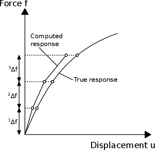
Figure 28: Drifting of the solution computed with a purely incremental method.

Thereby, in order to avoid the cited drifting, it is advisable to use an incremental-iterative (or prediction-correction) method. In essence, one must compute a prediction of the solution, and then correct it by means of iterations (see Figure 29). Each load level must be seen as a new non-linear problem that requires iterations to converge.

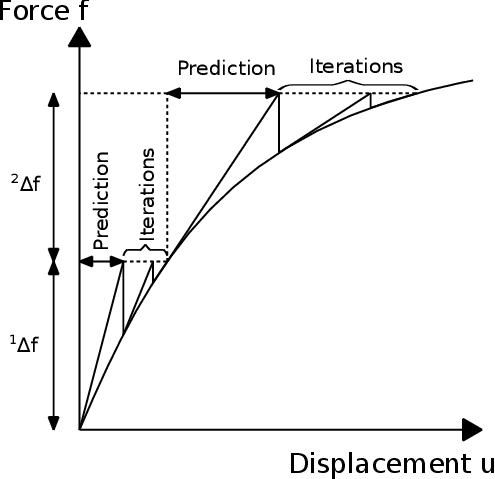
Figure 29: Example of an incremental-iterative method. Drifting is avoided.

The most commonly used iterative methods are the Picard's method and the Newton-Raphson's method. The first one is based on the secant matrix method, whereas the latter relies on the tangent matrix method.

Picard's method is very simple. At the beginning of a step ${\textstyle n+1}$ we must compute the prediction like:

${^{n+1}{\boldsymbol {a}}}^{0}=[{\boldsymbol {K}}_{sec}(^{n}{\boldsymbol {a}})]^{-1}\,[{^{n+1}}{\boldsymbol {f}}_{ext}]$

(147)

After that, we must correct that prediction by iterating. At a generic iteration ${\textstyle i+1}$ we have:

${^{n+1}{\boldsymbol {a}}}^{i+1}=[{\boldsymbol {K}}_{sec}(^{n+1}{\boldsymbol {a}}^{i})]^{-1}\,[{^{n+1}}{\boldsymbol {f}}_{ext}]$

(148)

Note that the superscript on the right of a variable represents the iteration number, whereas the superscript on the left shows the load step.

Thereby, at the end of each iteration we need to check the convergence criterion. A good option is to check a ratio of displacements and a ratio of residuals:

${\frac {\|{^{n+1}{\boldsymbol {a}}}^{i+1}-{^{n+1}{\boldsymbol {a}}}^{i}\|}{\|{^{n+1}{\boldsymbol {a}}}^{i+1}\|}}\leq tolerance_{a}\quad ;\quad {\frac {\|{\boldsymbol {R}}(^{n+1}{\boldsymbol {a}}^{i+1})\|}{\|{\boldsymbol {R}}(^{n+1}{\boldsymbol {a}}^{0})\|}}\leq tolerance_{R}$

(149)

With Newton-Raphson's method, we start each step computing the prediction just like in Picard's method. In this case, though, it is calculated from an incremental update:

$^{n+1}{\boldsymbol {a}}^{0}={^{n}{\boldsymbol {a}}}+[{\boldsymbol {K}}_{tan}(^{n}{\boldsymbol {a}})]^{-1}\,[{^{n+1}\Delta }{\boldsymbol {f}}_{ext}]$

(150)

Since in Newton's method it is more convenient to work with increments of displacements, let us define the sought solution at step ${\textstyle n+1}$ and iteration ${\textstyle i+1}$ like:

${^{n+1}{\boldsymbol {a}}}^{i+1}={^{n+1}{\boldsymbol {a}}}^{i}+{^{n+1}\delta }{\boldsymbol {a}}^{i+1}$

(151)

The unknown ${\textstyle {^{n+1}\delta }{\boldsymbol {a}}^{i+1}}$ is obtained by linearizing the residual around ${\textstyle {^{n+1}{\boldsymbol {a}}}^{i}}$ and imposing equilibrium:

${\boldsymbol {R}}({\boldsymbol {a}}+\delta {\boldsymbol {a}})={\boldsymbol {R}}({\boldsymbol {a}})+{\frac {\partial {\boldsymbol {R}}}{\partial {\boldsymbol {a}}}}\delta {\boldsymbol {a}}+\dots ={\boldsymbol {0}}$

(152)

Considering conservative loads we have:

${\frac {\partial {\boldsymbol {R}}}{\partial {\boldsymbol {a}}}}={\frac {\partial {\boldsymbol {f}}_{int}}{\partial {\boldsymbol {a}}}}={\boldsymbol {K}}_{tan}$

and so from the relation in (152) we can write:

$^{n+1}\delta {\boldsymbol {a}}^{i+1}=-[{\boldsymbol {K}}_{tan}(^{n+1}{\boldsymbol {a}}^{i})]^{-1}{\boldsymbol {R}}(^{n+1}{\boldsymbol {a}}^{i})$

(153)

Substituting (153) in (151) we get the final expression for the sought solution at any iteration:

${^{n+1}{\boldsymbol {a}}}^{i+1}={^{n+1}{\boldsymbol {a}}}^{i}-[{\boldsymbol {K}}_{tan}(^{n+1}{\boldsymbol {a}}^{i})]^{-1}{\boldsymbol {R}}(^{n+1}{\boldsymbol {a}}^{i})$

(154)

Finally, at the end of each iteration we just need to check the convergence criterion with (149).

Comparing Picard's and Newton-Raphson's methods, we must say that the first is cheap and robust, but it shows linear convergence rate. The latter, on the other hand, is much more expensive and less robust, but shows quadratic convergence.

To finish this section, we will present the arc-length strategy implemented in this work.

3.3.2.2 Modified Riks-Wempner arc-length method

The arc-length method is a solution strategy in which the path through a converged solution, at any step, follows a direction orthogonal to the tangent of the solution curve. In this procedure, both the load vector and the displacement field vary.

Thereby, the main differential aspect of the arc-length method with respect to other incremental-iterative techniques is that the former introduces an additional scalar variable in the residual equation, in order to account for the variation of the load vector. In this regard, we should rewrite expression (135) like:

${\boldsymbol {R}}({\boldsymbol {a}},\lambda )={\boldsymbol {f}}_{int}({\boldsymbol {a}})-{\boldsymbol {f}}_{ext}(\lambda )={\boldsymbol {K}}_{sec}({\boldsymbol {a}}){\boldsymbol {a}}-\lambda {\boldsymbol {f}}={\boldsymbol {0}}$

(155)

where ${\textstyle \lambda }$ is the load-level parameter that will be considered as a new unknown of the problem.

As a result, we have ${\textstyle N+1}$ degrees of freedom from the vector of nodal displacements ${\textstyle {\boldsymbol {a}}}$ and the load-level parameter ${\textstyle \lambda }$, but we only have ${\textstyle N}$ equations in (155). Therefore, we need an additional constraint equation to complete the definition of the problem:

$h({\boldsymbol {a}},\lambda )=0$

(156)

The form of the generic function ${\textstyle h(({\boldsymbol {a}},\lambda )}$ will depend on the chosen arc-length strategy. In our case, we chose the modified Riks-Wempner method (or Ramm's method).

In [55] Ramm proposed the following relation for (156):

$h({\boldsymbol {a}},\lambda )=[{^{n+1}\Delta }{\boldsymbol {a}}]^{T}\,[{^{n+1}\Delta }{\boldsymbol {a}}]+({^{n+1}\Delta }\lambda )^{2}-(\Delta S)^{2}=0$

(157)

where ${\textstyle \Delta S}$ is the arc-length increment, defined as the distance along the response curve ${\textstyle ({\boldsymbol {a}},\lambda )}$; and ${\textstyle {^{n+1}\Delta }{\boldsymbol {a}}}$ and ${\textstyle {^{n+1}\Delta }\lambda }$ are, respectively, the increments in the displacement field and load parameter from step ${\textstyle n}$ to step ${\textstyle n+1}$:

${^{n+1}\Delta }{\boldsymbol {a}}={^{n+1}{\boldsymbol {a}}}-{^{n}{\boldsymbol {a}}}\quad ;\quad {^{n+1}\Delta }\lambda ={^{n+1}\lambda }-{^{n}\lambda }$

(158)

In these equations ${\textstyle ({^{n}{\boldsymbol {a}}},{^{n}\lambda })}$ is the last converged equilibrium point on the curve ${\textstyle ({\boldsymbol {a}},\lambda )}$, whereas ${\textstyle ({^{n+1}{\boldsymbol {a}}},{^{n+1}\lambda })}$ is the converged equilibrium point after an increment of the arc-length ${\textstyle \Delta S}$ on the same curve.

Furthermore, Ramm limited the length of the displacement increment for the prediction of each step with:

$[^{n+1}\delta {\boldsymbol {a}}^{0}]^{T}[^{n+1}\delta {\boldsymbol {a}}^{0}]=\Delta S^{2}$

(159)

where ${\textstyle ^{n+1}\delta {\boldsymbol {a}}^{0}}$ is the displacement increment between the predicted point ${\textstyle {^{n+1}{\boldsymbol {a}}^{0}}}$ and the last converged equilibrium point ${\textstyle {^{n}{\boldsymbol {a}}}}$:

$^{n+1}\delta {\boldsymbol {a}}^{0}={^{n+1}{\boldsymbol {a}}^{0}}-{^{n}{\boldsymbol {a}}}$

(160)

Equation (159) represents that the incremental displacement of the prediction must fall on the hypersphere of radius ${\textstyle \Delta S}$ (see Figure 30).

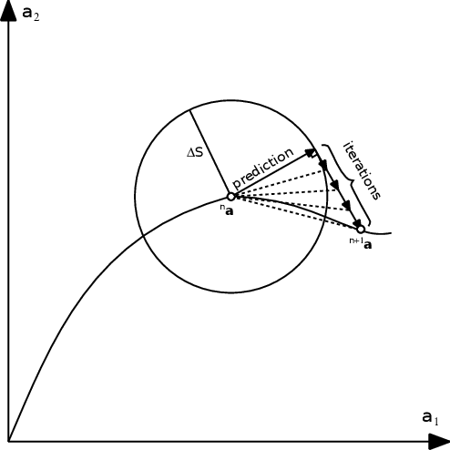
Figure 30: Ramm's method for a two degree of freedom system.

Thereby, with the modified Riks-Wempner method, the solution along the curve is found by following a line (or hyperplane) orthogonal to the prediction, which can be expressed by:

$[^{n+1}\delta {\boldsymbol {a}}^{0}]^{T}[^{n+1}\delta {\boldsymbol {a}}^{i+1}]=0$

(161)

After this short geometrical interpretation of the method, let us present the main steps of the algorithm.

Like we saw for the Newton-Raphson incremental-iterative technique, we start each step computing the prediction. However, since here we have the additional unknown ${\textstyle \lambda }$, we need to obtain a prediction for both the load factor and the displacement field.

Given a prescribed radius ${\textstyle ^{n+1}\Delta S}$, the prediction increment for the load factor is:

$^{n+1}\delta \lambda ^{0}={\frac {{^{n+1}\Delta }S}{\sqrt {[^{n+1}\delta {\boldsymbol {a}}_{f}^{0}]^{T}[^{n+1}\delta {\boldsymbol {a}}_{f}^{0}]}}}$

(162)

and the corresponding to the displacement field is:

$^{n+1}\delta {\boldsymbol {a}}^{0}=[{^{n+1}\delta }\lambda ^{0}][{^{n+1}\delta }{\boldsymbol {a}}_{f}^{0}]$

(163)

where

$^{n+1}\delta {\boldsymbol {a}}_{f}^{0}=[{\boldsymbol {K}}_{tan}(^{n}{\boldsymbol {a}})]^{-1}{\boldsymbol {f}}$

(164)

Again, in the arc-length method we have two unknowns, and so we define the sought solution for the displacement field like in Newton-Raphson's method (151), and the one for the load factor like:

${^{n+1}\lambda }^{i+1}={^{n+1}\lambda }^{i}+{^{n+1}\delta }\lambda ^{i+1}$

(165)

Thereby, as proposed by [56], we obtain ${\textstyle {^{n+1}\delta }{\boldsymbol {a}}^{i+1}}$ from two distinct parts:

${^{n+1}\delta }{\boldsymbol {a}}^{i+1}={^{n+1}\delta }{\boldsymbol {a}}_{R}^{i+1}+[{^{n+1}\delta }\lambda ^{i+1}][{^{n+1}\delta }{\boldsymbol {a}}_{f}^{i+1}]$

(166)

and we calculate ${\textstyle {^{n+1}\delta }\lambda ^{i+1}}$ from:

${^{n+1}\delta }\lambda ^{i+1}=-{\frac {[^{n+1}\delta {\boldsymbol {a}}^{0}]^{T}[{^{n+1}\delta }{\boldsymbol {a}}_{R}^{i+1}]}{[^{n+1}\delta {\boldsymbol {a}}^{0}]^{T}[{^{n+1}\delta }{\boldsymbol {a}}_{f}^{i+1}]}}$

(167)

where

${^{n+1}\delta }{\boldsymbol {a}}_{R}^{i+1}=[{\boldsymbol {K}}_{tan}(^{n+1}{\boldsymbol {a}}^{i})]^{-1}{\boldsymbol {R}}(^{n+1}{\boldsymbol {a}}^{i})$

(168)

and

${^{n+1}\delta }{\boldsymbol {a}}_{f}^{i+1}=[{\boldsymbol {K}}_{tan}(^{n+1}{\boldsymbol {a}}^{i})]^{-1}{\boldsymbol {f}}$

(169)

Finally, at the end of each iteration, we check the convergence criterion with (149).

As a concluding remark, we must say that Ramm's arc-length method is not the most accurate arc-length strategy, but offers the advantage of simplicity, and guarantees a solution as long as it physically exists.

We must also stress the importance of the arc-length radius ${\textstyle \Delta S}$, which controls the advancing velocity in the incremental-iterative process. The larger this radius, the faster is followed the equilibrium path. Nevertheless, near limit points with abrupt change in the response, an excessively large radius may lead to difficulties in tracing the load-displacement response. On the contrary, if the radius is chosen too small, the computational cost to obtain the solution path is very expensive. For this reason, in this work we have been estimating the radius with the relation proposed by Crisfield [57].

$^{n+1}\Delta S={^{n}\Delta }S\left({\frac {I_{d}}{^{n}I}}\right)^{1/2}$

(170)

where ${\textstyle I_{d}}$ is an input parameter of the desired number of iterations per step, and ${\textstyle ^{n}I}$ is the number of iterations at the previous step ${\textstyle n}$.

The above radius control leads to small increments when the response is most non-linear, and large increments when the response is most linear.

Moreover, in the first step we estimate the radius from:

$^{0}\Delta S={\sqrt {[^{0}\delta {\boldsymbol {a}}]^{T}[^{0}\delta {\boldsymbol {a}}]}}$

(171)

where

$^{0}\delta {\boldsymbol {a}}=[{\boldsymbol {K}}_{tan}(^{0}{\boldsymbol {a}})]^{-1}{\boldsymbol {R}}(^{0}{\boldsymbol {a}})$

(172)

with ${\textstyle ^{0}{\boldsymbol {a}}}$ being the initial guess of the displacement field.

3.4 Relevant Aspects on the Implementation of the Damage Models

In the following lines we will be reviewing how the main "ingredients" of the implemented arc-length strategy are obtained for the two implemented damage models: the partially regularized local damage model, and the fully regularized non-local damage model.

The main purpose of the section is to clarify the differences in the practical implementation of both models, pointing out those aspects that have not been mentioned in previous sections.

Looking at the expressions of the variables (168) and (169) defining the unknowns of the problem, one can see that at each iteration we need to know the tangent stiffness matrix ${\textstyle {\boldsymbol {K}}_{tan}(^{n+1}{\boldsymbol {a}}^{i})}$, the residual vector ${\textstyle {\boldsymbol {R}}(^{n+1}{\boldsymbol {a}}^{i})}$ and the vector of external forces ${\textstyle {\boldsymbol {f}}}$. Since we are working with conservative loads, this last vector is calculated only at the first step of the process. The tangent matrix and the residual vector, though, must be computed at each iteration.

The residual vector was presented in (155), with the vector of internal forces defined in terms of the secant stiffness matrix. In KRATOS, however, it is not computed using that form. Instead, the vector of internal forces is obtained by assembling the elementary contributions of an equivalent relation extracted from the Principle of Virtual Works (100):

${\boldsymbol {f}}_{int}^{(e)}({\boldsymbol {a}})=\iint _{A^{(e)}}{\boldsymbol {B}}^{T}{\boldsymbol {\sigma }}\,tdA$

(173)

where ${\textstyle {\boldsymbol {\sigma }}}$ is the stress vector.

Thereby, in order to clearly understand the solution procedure followed in the implemented damage models, in the next paragraphs we will be assessing how to compute the stress vector and the tangent stiffness matrix at each iteration, for the partially regularized local damage model, and for the non-local damage approach.

3.4.1 Partially regularized local damage model

When computing the elementary contributions of the vector of internal forces (173), it is necessary to calculate the stress vector at each integration point.

In the partially regularized damage model, this procedure is very straightforward because it is performed like in any classical isotropic damage model. Thereby, we can obtain the stresses at any integration point from the locally evaluated strains and damage parameter (see Table 1).

As mentioned in the previous section, the expression for the elemental tangent stiffness matrix can be derived from the same definition of the internal forces (173):

${\boldsymbol {K}}_{tan}^{(e)}$ $={\frac {\partial {\boldsymbol {f}}_{int}^{(e)}}{\partial {\boldsymbol {a}}}}={\frac {\partial }{\partial {\boldsymbol {a}}}}\left[\iint _{A^{(e)}}{\boldsymbol {B}}^{T}{\boldsymbol {\sigma }}\,tdA\right]$ $=\iint _{A^{(e)}}{\frac {\partial {\boldsymbol {B}}^{T}}{\partial {\boldsymbol {a}}}}{\boldsymbol {\sigma }}\,tdA+\iint _{A^{(e)}}{\boldsymbol {B}}^{T}{\frac {\partial {\boldsymbol {\sigma }}}{\partial {\boldsymbol {a}}}}\,tdA$

(174)

Thereby, since the problem we are solving falls into the material non-linearity category and we are working in a small deformation regime we have:

${\frac {\partial {\boldsymbol {B}}^{T}}{\partial {\boldsymbol {a}}}}={\boldsymbol {0}}\quad ;\quad {\frac {\partial {\boldsymbol {\sigma }}}{\partial {\boldsymbol {a}}}}={\frac {\partial {\boldsymbol {\sigma }}}{\partial {\boldsymbol {\varepsilon }}}}{\frac {\partial {\boldsymbol {\varepsilon }}}{\partial {\boldsymbol {a}}}}$

(175)

Now, taking into account the relations (47) and (92) we can write:

${\frac {\partial {\boldsymbol {\sigma }}}{\partial {\boldsymbol {\varepsilon }}}}={\boldsymbol {E}}_{tan}\quad ;\quad {\frac {\partial {\boldsymbol {\varepsilon }}}{\partial {\boldsymbol {a}}}}={\boldsymbol {B}}$

(176)

And so (174) can be rewritten as:

${\boldsymbol {K}}_{tan}^{(e)}=\iint _{A^{(e)}}{\boldsymbol {B}}^{T}{\boldsymbol {E}}_{tan}{\boldsymbol {B}}\,tdA$

(177)

where ${\textstyle {\boldsymbol {E}}_{tan}}$ is the tangent constitutive tensor that we presented in section 2.2.4.

It is interesting to notice that from expression (177) one obtains the the tangent stiffness matrix, but only by substituting the tangent constitutive tensor by the secant one ${\textstyle {\boldsymbol {E}}_{sec}}$, one obtains the secant stiffness matrix (see 131).

Figure 31 shows the general scheme followed in the local damage model for obtaining the stress vector and the tangent stiffness matrix at any iteration.

Figure 31: General scheme for the evaluation of the stress vector and the tangent stiffness matrix at any iteration of the local damage model.

3.4.2 Integral-type non-local damage model

Numerical implementation of the non-local damage model based on averaging of equivalent strain is relatively simple. The evaluation of stresses remains explicit, and no internal iteration is needed. All that one needs is to implement the algorithm of weighted spatial averaging and, before damage is evaluated, replace the local equivalent strain by its non-local counterpart.

The values of non-local equivalent strain must be traced at individual Gauss integration points of the finite element model, because these are the points at which stresses need to be evaluated.

Thereby, the averaging integral in (63), defining the non-local equivalent strain at a given integration point, is evaluated numerically. Thus, considering the weighting function defined in (62), we have:

${\tilde {\varepsilon }}_{eq}({\boldsymbol {x}}_{p})=\sum _{q}w_{q}\alpha _{pq}\varepsilon _{eq}({\boldsymbol {x}}_{q})$

(178)

where ${\textstyle w_{q}}$ is a coefficient containing the product of the determinant of the Jacobian, the thickness, and the integration weights of Gauss point ${\textstyle q}$; ${\textstyle {\boldsymbol {x}}_{q}}$ are the coordinates of the integration point; and ${\textstyle \alpha _{pq}}$ is the weight of non-local interaction between points ${\textstyle p}$ and ${\textstyle q}$, defined as:

$\alpha _{pq}={\frac {\alpha _{0}(\|{\boldsymbol {x}}_{p}-{\boldsymbol {x}}_{q}\|)}{\sum _{r}w_{r}\alpha _{0}(\|{\boldsymbol {x}}_{p}-{\boldsymbol {x}}_{r}\|)}}$

(179)

In the previous two equations, subscript ${\textstyle p}$ represents the receiver point under consideration, that can be any integration point in the solid domain, whereas indexes ${\textstyle q}$ and ${\textstyle r}$ correspond to source points. Furthermore, since the chosen weighting function ${\textstyle \alpha _{0}}$ has bounded support (59), ${\textstyle \alpha _{pq}}$ vanishes if the distance ${\textstyle \|{\boldsymbol {x}}_{p}-{\boldsymbol {x}}_{q}\|}$ between points ${\textstyle p}$ and ${\textstyle q}$ is larger than the interaction radius ${\textstyle R}$. Therefore, the sums in (178) and (179) do not need to be taken over all Gauss points, but only over those that are located inside the domain of influence of point ${\textstyle p}$. In this regard we must notice that, in order to account for the non-local interaction, at the damage process zone one must always use an element size smaller than the interaction radius. Otherwise the damage model would become local.

Therefore, each Gauss point must have a non-local interaction table that gives access to its neighbours. This table must be constructed, at the beginning of the problem, from a search of non-local neighbours.

In this work, the search of neighbours is performed by means of a grid-based algorithm. A general rectangular grid is defined in the entire domain and all the integration points are positioned in the cells. This way, the neighbour search that must be performed for each Gauss point is restricted to a limited number of cells, i.e., the ones that fall inside the interaction radius of the considered point (see Figure 32).

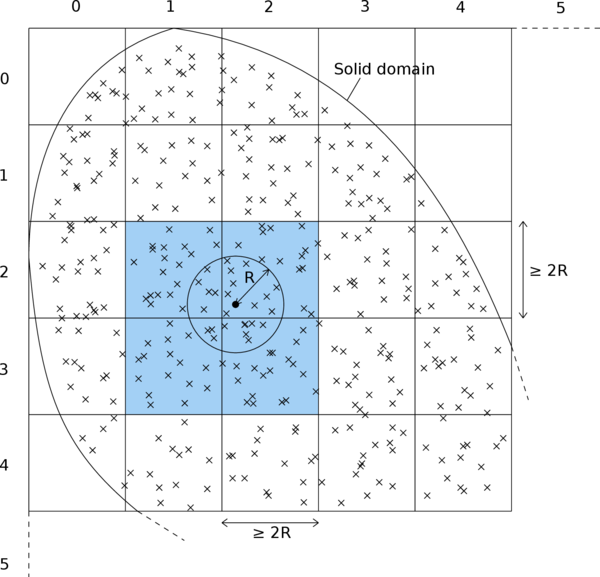
Figure 32: Grid-based non-local search.

The stress evaluation procedure, repeatedly called during the incremental-iterative strategy, makes use of the non-local interaction tables when the non-local equivalent strain is computed. To obtain ${\textstyle {\tilde {\varepsilon }}_{eq}}$, we first compute the local equivalent strains at all Gauss points, and then we calculate the non-local counterpart using (178).

With regard to the stiffness matrix, if one aims to obtain an iterative solver with quadratic convergence when working with a non-local damage model, it is necessary to construct the tangent stiffness matrix in a consistent manner.

Let us start rewriting the expression for the vector of internal forces (173) as a numerical integration over Gauss points:

${\boldsymbol {f}}_{int}=\sum _{p}w_{p}{\boldsymbol {B}}^{T}({\boldsymbol {x}}_{p}){\boldsymbol {\sigma }}({\boldsymbol {x}}_{p})$

(180)

Using the stress-strain law (128) and the standard strain-displacement relation (92), we can expand (180) as follows:

${\boldsymbol {f}}_{int}$ $=\sum _{p}w_{p}(1-d_{p}){\boldsymbol {B}}_{p}^{T}{\boldsymbol {E}}{\boldsymbol {B}}_{p}{\boldsymbol {a}}$ $=\sum _{p}w_{p}(1-d_{p}){\boldsymbol {K}}_{p}{\boldsymbol {a}}$

(181)

where ${\textstyle {\boldsymbol {K}}_{p}={\boldsymbol {B}}_{p}^{T}{\boldsymbol {E}}{\boldsymbol {B}}_{p}}$. In the virgin state ${\textstyle d_{p}=0}$ at all integration points and so (181) can be rewritten as ${\textstyle {\boldsymbol {f}}_{int}={\boldsymbol {K}}{\boldsymbol {a}}}$, where ${\textstyle {\boldsymbol {K}}=\sum _{p}w_{p}{\boldsymbol {K}}_{p}}$ is the elastic stiffness matrix.

As we have already said, the tangent stiffness matrix is obtained by differentiating the internal forces with respect to the nodal displacements. Since the damage variable depends on the nodal displacements through the equivalent strain, we will need to compute first the derivative of the damage variable with respect to the displacement vector ${\textstyle {\boldsymbol {a}}}$. Taking into account that ${\textstyle d=g(r)}$ (7), ${\textstyle r}$ depends on ${\textstyle {\tilde {\varepsilon }}_{eq}}$ (64), and ${\textstyle {\tilde {\varepsilon }}_{eq}}$ depends on ${\textstyle {\boldsymbol {a}}}$ through the interpolated strains, we can use the chain rule to write the derivative of the damage variable for an integration point ${\textstyle p}$ as follows:

${\frac {\partial d_{p}}{\partial {\boldsymbol {a}}}}={\frac {dg}{dr_{p}}}{\frac {dr_{p}}{d{\tilde {\varepsilon }}_{eq,p}}}{\frac {\partial {\tilde {\varepsilon }}_{eq,p}}{\partial {\boldsymbol {a}}}}=g'_{p}t_{p}{\frac {\partial {\tilde {\varepsilon }}_{eq,p}}{\partial {\boldsymbol {a}}}}$

(182)

where ${\textstyle g'_{p}}$ is the derivative of the damage evolution law with respect to the internal state variable ${\textstyle r}$, and ${\textstyle t_{p}}$ is the loading-unloading factor that is 0 in an elastic loading or in an unloading regime, and 1 in a loading regime with growing damage:

$t={\frac {dr}{d{\tilde {\varepsilon }}_{eq}}}=\left\{{\begin{array}{ll}0&{\hbox{if }}{\tilde {\varepsilon }}_{eq}<r{\hbox{ }}\\1&{\hbox{if }}{\tilde {\varepsilon }}_{eq}=r{\hbox{ and }}{\dot {\tilde {\varepsilon }}}_{eq}\geq 0{\hbox{ }}\end{array}}\right.$

(183)

Now, from expression (178), we can differentiate the non-local equivalent strain of a Gauss point ${\textstyle p}$ with respect to the nodal displacements:

${\frac {\partial {\tilde {\varepsilon }}_{eq,p}}{\partial {\boldsymbol {a}}}}=\sum _{q}w_{q}\alpha _{pq}{\frac {\partial \varepsilon _{eq,q}}{\partial {\boldsymbol {a}}}}$

(184)

And by using the chain rule and the relation in (92) we obtain:

${\frac {\partial {\tilde {\varepsilon }}_{eq,p}}{\partial {\boldsymbol {a}}}}=\sum _{q}w_{q}\alpha _{pq}{\frac {\partial \varepsilon _{eq,q}}{\partial {\boldsymbol {\varepsilon }}_{q}}}{\frac {\partial {\boldsymbol {\varepsilon }}_{q}}{\partial {\boldsymbol {a}}}}=\sum _{q}w_{q}\alpha _{pq}{\frac {\partial \varepsilon _{eq,q}}{\partial {\boldsymbol {\varepsilon }}_{q}}}{\boldsymbol {B}}_{q}$

(185)

the derivative of the equivalent strain with respect to the strain components ${\textstyle \partial \varepsilon _{eq,q}/\partial {\boldsymbol {\varepsilon }}_{q}}$ is a row matrix that will depend on the chosen form of equivalent strain.

Let us now rewrite the expression of the internal forces in (181) as follows:

${\boldsymbol {f}}_{int}=\sum _{p}w_{p}{\boldsymbol {K}}_{p}{\boldsymbol {a}}-\sum _{p}w_{p}{\boldsymbol {K}}_{p}{\boldsymbol {a}}d_{p}$

(186)

At this point, we can already differentiate (186) and substitute (182) to get a first expression for the tangent stiffness matrix.

${\boldsymbol {K}}_{tan}$ $={\frac {\partial {\boldsymbol {f}}_{int}}{\partial {\boldsymbol {a}}}}=\sum _{p}w_{p}{\boldsymbol {K}}_{p}-\left(\sum _{p}w_{p}{\boldsymbol {K}}_{p}d_{p}+\sum _{p}w_{p}{\boldsymbol {K}}_{p}{\boldsymbol {a}}{\frac {\partial d_{p}}{\partial {\boldsymbol {a}}}}\right)$ $=\sum _{p}w_{p}(1-d_{p}){\boldsymbol {K}}_{p}-\sum _{p}w_{p}{\boldsymbol {K}}_{p}{\boldsymbol {a}}{\frac {\partial d_{p}}{\partial {\boldsymbol {a}}}}$ $=\sum _{p}w_{p}{\boldsymbol {B}}_{p}^{T}(1-d_{p}){\boldsymbol {E}}{\boldsymbol {B}}_{p}-\sum _{p}w_{p}{\boldsymbol {B}}_{p}^{T}{\boldsymbol {E}}{\boldsymbol {B}}_{p}{\boldsymbol {a}}g'_{p}t_{p}{\frac {\partial {\tilde {\varepsilon }}_{eq,p}}{\partial {\boldsymbol {a}}}}$

(187)

Note that the first term is the secant stiffness matrix, that coincides with the tangent matrix in an elastic loading or in an unloading regime (${\textstyle t_{p}=0}$ ${\textstyle \forall p}$). The term on the right is the non-local part of the tangent stiffness matrix which, substituting (185), results:

${\boldsymbol {K}}_{tan}$ $={\boldsymbol {K}}_{sec}-\sum _{p}w_{p}{\boldsymbol {B}}_{p}^{T}{\boldsymbol {E}}{\boldsymbol {\varepsilon }}_{p}g'_{p}t_{p}\sum _{q}w_{q}\alpha _{pq}{\frac {\partial \varepsilon _{eq,q}}{\partial {\boldsymbol {\varepsilon }}_{q}}}{\boldsymbol {B}}_{q}$ $={\boldsymbol {K}}_{sec}-\sum _{p,q}w_{p}{\boldsymbol {B}}_{p}^{T}{\boldsymbol {\bar {\sigma }}}_{p}g'_{p}t_{p}w_{q}\alpha _{pq}{\frac {\partial \varepsilon _{eq,q}}{\partial {\boldsymbol {\varepsilon }}_{q}}}{\boldsymbol {B}}_{q}$

(188)

Defining for convenience the column matrix ${\textstyle {\boldsymbol {b}}_{p}^{c}={\boldsymbol {B}}_{p}^{T}{\boldsymbol {\bar {\sigma }}}_{p}}$, the row matrix ${\textstyle {\boldsymbol {b}}_{q}^{r}=\displaystyle {\frac {\partial \varepsilon _{eq,q}}{\partial {\boldsymbol {\varepsilon }}_{q}}}{\boldsymbol {B}}_{q}}$, and the coefficient ${\textstyle w_{pq}=w_{p}w_{q}\alpha _{pq}}$, (188) can be rewritten like:

${\boldsymbol {K}}_{tan}={\boldsymbol {K}}_{sec}-\sum _{p,q}w_{pq}g'_{p}t_{p}{\boldsymbol {b}}_{p}^{c}{\boldsymbol {b}}_{q}^{r}$

(189)

The double index of the sum, caused by the non-local interaction, implies that the term on the right part of the expression (189) cannot be assembled from elementary contributions solely. Essentially, each pair of Gauss points ${\textstyle p}$ and ${\textstyle q}$ contributes to the global stiffness matrix with a block of the same size as that of the classical element stiffness matrix. The difference is that the assembling routine differs from the usual one because in this case one needs to take into account the elements of both points ${\textstyle p}$ and ${\textstyle q}$ (see Figure 33). In consequence, the global stiffness matrix is always non-symmetric and its bandwidth increases due to the non-local interaction.

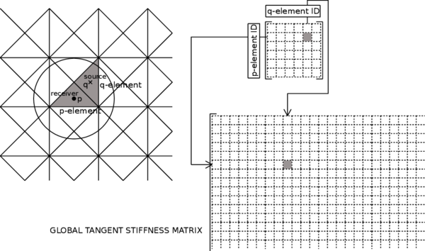
Figure 33: Assembly of non-local contributions to the global tangent stiffness matrix.

In order to avoid the additional non-zero entries that the non-local interaction introduces into the global stiffness matrix, some authors neglect the non-local terms by using ${\textstyle \alpha _{pq}=\delta _{pq}/w_{p}}$, where ${\textstyle \delta _{pq}}$ is the Kronecker delta, and so ${\textstyle w_{pq}=\delta _{pq}w_{q}}$. This way, equation (189) reduces to:

${\boldsymbol {K}}_{tan}^{local}={\boldsymbol {K}}_{sec}-\sum _{p}w_{p}g'_{p}t_{p}{\boldsymbol {b}}_{p}^{c}{\boldsymbol {b}}_{p}^{r}$

(190)

in essence, the sum is performed over one index only. However, it must be noticed that the resulting local tangent matrix ${\textstyle {\boldsymbol {K}}_{tan}^{local}}$ is no longer consistent, and quadratic convergence is lost. Furthermore, although the secant matrix is always symmetric, the corrective term on the right part of expression (190) is symmetric only if the column matrix ${\textstyle {\boldsymbol {b}}^{c}}$ and the row matrix ${\textstyle {\boldsymbol {b}}^{r}}$ are linearly dependent, which is the case if ${\textstyle \partial \varepsilon _{eq}/\partial {\boldsymbol {\varepsilon }}}$ is a scalar multiple of the effective stresses ${\textstyle {\boldsymbol {\bar {\sigma }}}}$. This is only true for the definition of the equivalent strain based on the damage energy release rate (19).

Therefore, the most important issue caused by non-locality is the evolutionary character of the profile of the stiffness matrix. For the simulation of quasi-brittle materials like concrete, the consistent stiffness matrix remains local through the elastic branch, and so the initial distribution of non-zero entries is the same as in the local case. Nevertheless, when the damage threshold is exceeded and the damage zone starts propagating, new non-zero entries appear due to the non-local interaction between Gauss points belonging to different elements, and the profile of the stiffness matrix must be dynamically adapted. The number of additional non-zero entries will depend on each particular case, but if a finer mesh is used in the expected softening zones, this number can be relatively high.

In conclusion, it must be noticed that non-local averaging certainly increases the computational cost with respect to the corresponding local model, but since the non-local model completely removes the pathological sensitivity to the mesh size, and partially alleviates the mesh-induced directional bias, this extra effort is indeed worthwhile.

Figure 34 shows the general scheme followed in the non-local damage model for obtaining the stress vector and the tangent stiffness matrix at any iteration.

Figure 34: General scheme for the evaluation of the stress vector and the tangent stiffness matrix at any iteration of the non-local damage model.

3.5 Mesh-Adaptive Technique

Non-local models lead to smooth solutions with a continuous variation of strain. However, to resolve narrow bands of highly localized strains, it is necessary to use sufficiently fine computational grids. Fortunately, the mesh must be fine only in the process zone, while the remaining part of the structure can be reasonably well represented by a coarser mesh. In general, the localization pattern is not known in advance, and it is actually tedious to construct suitably refined meshes by hand. Thereby, efficiency of the analysis can be greatly increased by means of an adaptive technique, which automates the whole process.

In this regard, one of the last implementations of this work has been an adaptive mesh refinement technique. Although still under development, it has already shown some interesting results, and so in this section we wanted to review the most important features of the procedure.

The starting point for the implementation of this adaptive technique was the work done by Miquel Portabella in its minor thesis [58]. The adaptive mesh refinement technique of Portabella was aimed at static-linear-elastic two-dimensional cases, and so we had to adapt it to incremental-iterative damage mechanics problems. Due to the importance of achieving robust results regardless of the mesh, we have designed this adaptive technique for the non-local damage method.

In the following lines, we will present the general structure of the adaptive procedure, and then its basic stages will be briefly discussed.

The general algorithm of non-linear adaptive analysis can be described as follows. After reaching the equilibrium state and updating the solution, an error estimation is performed in order to evaluate the error distribution over the mesh. Then, a remeshing criterion uses the information about error distribution and determines the required mesh density. From this analysis, we can obtain a new spatial discretization using a mesh generator interface.

In a truly adaptive approach, after generating a new discretization, the data structures corresponding to the newly generated mesh are created, and the transfer of displacements and internal variables from the old mesh to the new one is performed. After the mapping, the internal variables are used together with the strain computed from the mapped displacements to update the internal state of each integration point on the new mesh (to achieve local consistency). Once the transfer has finished, the old discretization is deleted and the mapped configuration is brought into global equilibrium through iteration. Afterwards, the solution continues with the next incremental-iterative step.

Another possibility is to restart the analysis from the initial state after the new discretization is generated. This approach does not require the transfer of the current state from the old discretization to the new one, but from the computational point of view is less efficient than the truly adaptive approach, especially if the remeshing is done frequently.

Let us now present the main stages of the implemented adaptive procedure, pointing out the most relevant aspects of each one:

• Error Estimation

The implemented error estimator is based on the stress evaluation. Thus, let us define the error as the difference between an exact value of effective stresses ${\textstyle {\bar {\boldsymbol {\sigma }}}_{e}}$ and an approximate one ${\textstyle {\bar {\boldsymbol {\sigma }}}_{a}}$:

${\boldsymbol {\epsilon }}_{\bar {\sigma }}={\bar {\boldsymbol {\sigma }}}_{e}-{\bar {\boldsymbol {\sigma }}}_{a}$

(191)

Since the Finite Element Method is an approximate technique, it is not possible to know the exact value of stresses. Thereby, we must estimate the error and substitute the exact value of effective stresses by a "reasonably good" value of stresses. This reasonably good value is obtained from the extrapolation of the stresses to the nodes, and posterior smoothing [59]. The approximate value of stresses is simply the default evaluated stresses of the FEM solution. Therefore, the estimated error can be defined as the difference between the smoothed effective stresses ${\textstyle {\bar {\boldsymbol {\sigma }}}_{s}}$, and the calculated effective stresses ${\textstyle {\bar {\boldsymbol {\sigma }}}}$:

${\boldsymbol {\epsilon }}_{\bar {\sigma }}\approx {\bar {\boldsymbol {\sigma }}}_{s}-{\bar {\boldsymbol {\sigma }}}$

(192)

However, we will be working with integral measures of the error that take into account the error over all the element, and so we define the energetic norm of the error over an element as:

$\|{\boldsymbol {\epsilon }}_{\bar {\sigma }}\|^{(e)}$ $=\left[\int _{\Omega ^{(e)}}{\boldsymbol {\epsilon }}_{\bar {\sigma }}^{T}{\boldsymbol {E}}^{-1}{\boldsymbol {\epsilon }}_{\bar {\sigma }}d\Omega \right]^{1/2}$ $=\left[\int _{\Omega ^{(e)}}[{\bar {\boldsymbol {\sigma }}}_{s}-{\bar {\boldsymbol {\sigma }}}]^{T}{\boldsymbol {E}}^{-1}[{\bar {\boldsymbol {\sigma }}}_{s}-{\bar {\boldsymbol {\sigma }}}]d\Omega \right]^{1/2}$

(193)

And, the square of the global error can be obtained from the sum of the squares of all the elemental errors:

$\|{\boldsymbol {\epsilon }}_{\bar {\sigma }}\|^{2}=\sum _{e}(\|{\boldsymbol {\epsilon }}_{\bar {\sigma }}\|^{(e)})^{2}$

(194)

The smaller is the distance between the nodes of the mesh, the smaller will be the difference between the smoothed and non-smoothed stresses. Thereby, the presented energetic norm tends to zero as the size of the element diminishes, i.e., ${\textstyle \|{\boldsymbol {\epsilon }}_{\bar {\sigma }}\|={\mathcal {O}}(h^{m})}$ where ${\textstyle h}$ is the element size and ${\textstyle m}$ is the order of the polynomial defining the shape functions.

• Remeshing Criterion

Determining whether a mesh must be refined or not requires to previously define some quality conditions based on the estimated error.

First, the energetic norm of the global error should be smaller than a certain percentage of the deformation energy:

$\|{\boldsymbol {\epsilon }}_{\bar {\sigma }}\|\leq \eta \,U$

(195)

where ${\textstyle \eta }$ is the permissible percentage of global error, and the deformation energy is obtained from:

$U^{2}=\sum _{e}(U^{(e)})^{2}$

(196)

with

$U^{(e)}=\left[\int _{\Omega ^{(e)}}{\bar {\boldsymbol {\sigma }}}_{s}^{T}{\boldsymbol {E}}^{-1}{\bar {\boldsymbol {\sigma }}}_{s}d\Omega \right]^{1/2}$

(197)

To determine whether condition (195) is fulfilled, it is convenient to work with a global error parameter defined as:

$\xi _{g}={\frac {\|{\boldsymbol {\epsilon }}_{\bar {\sigma }}\|}{\eta \,U}}$

(198)

Thereby, when ${\textstyle \xi _{g}=1}$ the global error condition is perfectly fulfilled, for ${\textstyle \xi _{g}>1}$ mesh should be refined, and for ${\textstyle \xi _{g}<1}$ the mesh size could be larger.

Furthermore, taking into account that ${\textstyle \|{\boldsymbol {\epsilon }}_{\bar {\sigma }}\|={\mathcal {O}}(h^{m})}$, the new element size ${\textstyle {\hat {h}}^{(e)}}$ can be obtained with:

${\hat {h}}^{(e)}={\frac {h^{(e)}}{(\xi _{g})^{\frac {1}{m}}}}$

(199)

If one aims at obtaining a selective refinement method, apart from (195), another condition concerning the error of each element must be simultaneously imposed. Depending on this local error condition, one can define different approaches [60,61]. In this work, we have been working with a remeshing criterion based on global error equidistribution.

This criterion distributes the global error uniformly among all the elements of the mesh, and so the elemental error should accomplish the following condition:

$\|{\boldsymbol {\epsilon }}_{\bar {\sigma }}\|^{(e)}\leq {\frac {\|{\boldsymbol {\epsilon }}_{\bar {\sigma }}\|}{\sqrt {n}}}$

(200)

where ${\textstyle n}$ is the number of elements of the mesh.

Like in the case of the global error, we can work with a local error parameter:

$\xi _{l}^{(e)}={\frac {{\sqrt {n}}\,\|{\boldsymbol {\epsilon }}_{\bar {\sigma }}\|^{(e)}}{\|{\boldsymbol {\epsilon }}_{\bar {\sigma }}\|}}$

(201)

with the same meaning that in the global case: ${\textstyle \xi _{l}^{(e)}=1}$ indicates an optimal element size, whereas ${\textstyle \xi _{l}^{(e)}>1}$ and ${\textstyle \xi _{l}^{(e)}<1}$ imply that the element is too large and too small, respectively.

This local parameter allows to define the new element size that accomplish (200):

${\hat {h}}^{(e)}={\frac {h^{(e)}}{(\xi _{l}^{(e)})^{\frac {2}{2m+d}}}}$

(202)

where ${\textstyle d}$ is the dimension of the problem.

In the end, the remeshing criterion results from the combination of the global error condition (195) and the local one (200). In consequence, the final refinement parameter of the element can be defined as:

$\xi ^{(e)}=\xi _{g}\,\xi _{l}^{(e)}={\frac {{\sqrt {n}}\,\|{\boldsymbol {\epsilon }}_{\bar {\sigma }}\|^{(e)}}{\eta \,U}}$

(203)

And the new element size is obtained with:

${\hat {h}}^{(e)}={\frac {h^{(e)}}{\gamma ^{(e)}}}$

(204)

where

$\gamma ^{(e)}=(\xi _{g})^{\frac {1}{m}}\,(\xi _{l}^{(e)})^{\frac {2}{2m+d}}$

(205)

• Mesh Generator Interface

The mesh generator interface is the one from GiD, a pre-processing and post-processing software. Therefore, not only GiD meshes the geometry in the beginning of a problem, but it is also GiD which allows to obtain the new spatial discretization every time we need to adapt the mesh.

Thereby, after the error estimator and the remeshing criterion are applied, a "background mesh" file (*.bgm) is generated with the information of the new element sizes. Then, GiD allows loading this background mesh file along with the original mesh file so as to generate a new mesh according to the refinement parameter of each old element.

Furthermore, before starting any problem, one can always change GiD meshing preferences in order to modify the velocity of mesh transition and other parameters that will affect the original mesh as well as the subsequent adapted meshes.

• Mapping of Variables

Before one can continue with the solution of a problem, there is a last stage that must be performed in a truly adaptive approach: the mapping of primary unknowns and internal variables.

In essence, if one aims at continuing the analysis from the current state, instead of restarting it from scratch after every mesh refinement, it is necessary to apply some transfer algorithms for the displacements and internal history variables (in the present case, the state variable ${\textstyle r}$ governing the damage evolution).

Mapping of the primary unknowns (nodal displacements) is achieved by using the shape function projections. To do so, we must first place each new node inside an old element, by means of a grid-based search, and then we interpolate the displacements of the old nodes to the new one (see Figure 35.a).

On the other hand, mapping of the internal state variables is done through a weighted spatial averaging, similar to the one used for the computation of the non-local equivalent strain. The difference is that, in this case, the source points are the integration points of the old mesh, and the receiver points are the integration points of the new mesh (see Figure 35.b). Like before, another grid-based search is performed in order to determine the Gauss points of the old mesh that fall inside the interaction radius ${\textstyle R}$ of each new Gauss point.

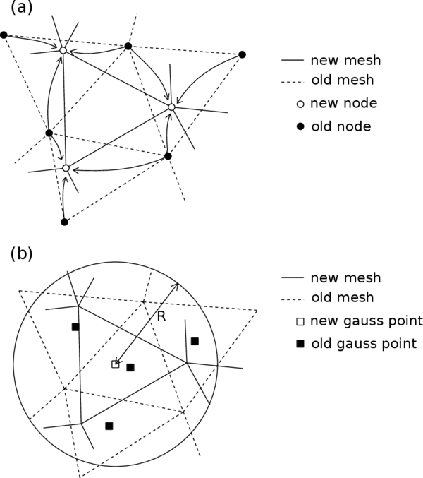
Figure 35: Mapping of variables: (a)Nodal displacements mapping. (b)Internal state variables mapping.

4 Examples

4.1 Introduction

At this point, we have already presented the fundamental concepts on damage mechanics theory, as well as the the most relevant aspects concerning the implementation of a damage model within the Finite Element Method.

The present chapter will be devoted to test and validate the implemented code, by solving two classical examples in the damage mechanics field: the three-point bending test, and the single-edge notched beam test.

For each one of the tests, two experiments will be performed. First, we will solve the problem with the two implemented damage models: the partially regularized local damage model, and the integral-type non-local damage model. The objective of this experiment is to analyse and compare both models, pointing out the strengths and limitations of the codes, and try to confirm that the non-local procedure is a valid and robust approach.

After that, we will solve the problem again, applying the implemented mesh-adaptive procedure to the non-local damage model. As we have already commented, this technique is still under development, but the examples performed will help us understand better the adaptive procedure and establish the next steps in its future evolution.

Both examples will be carried out in 2D, which is actually advantageous when testing a new code, given its reduced computational cost as compared to the corresponding three-dimensional case. Thereby, as we stated before, we will be using three-node triangular elements and four-node quadrilateral elements to represent the discretized domain. Regarding the solving strategy, we will be working with the arc-length method presented in the previous chapter, and thus we will be following the equilibrium path of the problems for a set of steps. Apart from that, self weight will not be considered in any of the examples.

Now, in order to properly understand the scheme followed for the performance of the examples, let us briefly present GiD.

GiD is a software for the pre-processing and post-processing of simulations. It has CAD tools for drawing the geometry, as well as a mesh generator for obtaining the spatial discretization of the model. Furthermore, GiD allows embedding customized modules specifically designed for a problem of interest, called "Problem Types", which enhance GiD pre-processing capacities so as to define all the relevant components of the model, i.e., boundary conditions, loads, material properties and computation parameters. In addition to this, the Problem Types are usually linked to the compiled KRATOS application that will solve the problem. Thereby, by using GiD along with an specific Problem Type, one can prepare a model and run the simulation from GiD itself. Lastly, GiD also offers post-processing tools, and so when the computation finishes, one can immediately display the obtained results in GiD. In essence, the solution of the problems follows the scheme in Figure 36.

Figure 36: Global structure for the solution of a problem.

4.2 Three-Point Bending Test

This test is performed with a notched beam subjected to three-point bending (TPB). The beam has a square cross section of 40 ${\textstyle \times }$ 320 mm, a span of 1280 mm, and the notch is 3 mm thick and extends over one tenth of the beam depth (see Figure 37).

Figure 37: TPB test. Problem statement. Distances in mm

In order to reduce fictitious stress concentrations at the supports and at the loading point, both the displacement constraints and the load are imposed over a line of 20 mm, as shown in Figure 38.

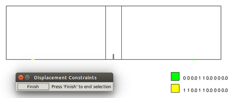
(a) Displacement constraints.

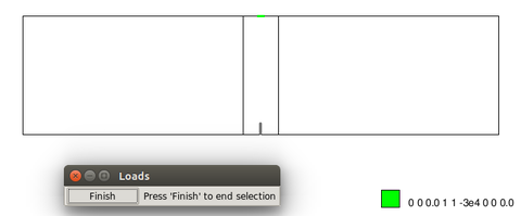
(b) Loads.

Figure 38: TPB test. Boundary Conditions.

In this case, plane stress conditions have been assumed, and the geometry will be meshed by means of standard four-node quadrilaterals with 2 ${\textstyle \times }$ 2 integration points.

4.2.1 Damage models testing

In this first experiment we will solve the problem using the two implemented damage models. On the one hand, the partially regularized local damage approach will make use of the modified version of the equivalent strain proposed by Simo and Ju (33), and the damage evolution law presented in (39). On the other hand, the non-local damage approach, will be defined with the Mazars model, regarding the equivalent strain (25) and the damage evolution law (42). The weighting function for the non-local interaction will depend on a Gauss distribution function of bounded support (59).

The material parameters for the local damage model are summarized in Table 5 and have been obtained after various attempts, trying to fit the experimental results in [62]. For the non-local approach we are going to use the material parameters obtained in [62] (see Table 6).

Table. 5 TPB test. Material parameters for the Simo-Ju local model.

Parameter	Value
Young's modulus (${\textstyle E}$)	38500 MPa
Poisson's ratio (${\textstyle \nu }$)	0.24
Compressive strength (${\textstyle \sigma _{y}^{c}}$)	45 MPa
Tensile strength (${\textstyle \sigma _{y}^{t}}$)	3.8 MPa
Fracture energy (${\textstyle G_{f}}$)	100 ${\textstyle J/m^{2}}$
Limit fracture length (${\textstyle l_{lim}}$)	5 mm

Table. 6 TPB test. Material parameters for the Mazars non-local model.

Parameter	Value
Young's modulus (${\textstyle E}$)	38500 MPa
Poisson's ratio (${\textstyle \nu }$)	0.24
Damage threshold (${\textstyle r_{0}}$)	${\textstyle 3\cdot {10}^{-5}}$
Parameter ${\textstyle A}$ in compression (${\textstyle A_{c}}$)	1.25
Parameter ${\textstyle B}$ in compression (${\textstyle B_{c}}$)	1000
Parameter ${\textstyle A}$ in tension (${\textstyle A_{t}}$)	0.95
Parameter ${\textstyle B}$ in tension (${\textstyle B_{t}}$)	9000
Characteristic length (${\textstyle l_{c}}$)	40 mm

In order to assess the robustness of the models in terms of mesh sensitivity, we are going to solve the problem for different spatial discretizations. Thereby, here we will be using three unstructured meshes of quadrilaterals with a minimum size of 15 mm, 7 mm, and 3 mm, respectively (see Figure 39).

(a) Mesh 1: 2024 elements, 2191 nodes.	(b) Mesh 2: 2679 elements, 2859 nodes.
(c) Mesh 3: 6543 elements, 6772 nodes.
Figure 39: TPB test. Spatial discretizations.

Figure 40 shows the relation between the applied load and the vertical deflection of the beam. As one can see from the discontinued equilibrium curves, we had serious difficulties in tracing the response of a full test. Once the limit point at the peak was surpassed, the ratio of residual forces would start oscillating without converging to the prescribed tolerance, even when reducing the arc-length radius. A stability study could reveal the presence of bifurcation points in the post-peak zone that should be carefully analysed in order to distinguish the stable branch (physically possible) from the unstable ones. However, another reason behind the convergence problems could be the use of a too global arc-length method, like the one implemented. Indeed, to account for the localized nature of quasi-brittle failure, a more specific control parameter, like the Crack Mouth Opening Displacement (CMOD), could help improving the convergence near snap-back zones.

That aside, if we look at the curves in Figure 40a we can see that, although there is no relevant difference between the response obtained with meshes 1 and 2, the peak actually decreases with the finest mesh 3, and so the total dissipated energy. On the other hand, the response diagram in Figure 40b shows practically the same peak load for the three meshes.

Thereby, only looking at the depicted curves, it seems that the partially regularized local damage model is more sensitive to changes in the spatial discretization than the non-local model.

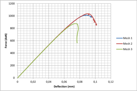
(a) Partially regularized local damage model.

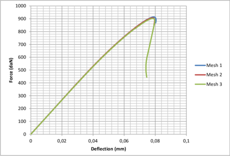
(b) Non-local damage model.

Figure 40: TPB test. Force-vertical deflection diagrams.

However, in order to understand better the response of both models, let us present some snapshots with the damage distribution.

Figures 41 and 43 show an initial stage of damage progression in the local and non-local model, respectively. Just by looking at the size and shape of the damaged zone, we can clearly state the most differential trait of each model: localization on the one hand, and diffusion on the other. This concept is crucial to understand the behaviour seen in the load-deflection diagrams of Figure 40.

Essentially, in the local approach, damage starts at the most stressed element and then "jumps" to the next one when the first is totally damaged. As a result, shape and direction of progression of damage strongly depends on the size and distribution of the elements of the mesh (see Figure 42).

(a) Mesh 1.

(b) Mesh 2.

(c) Mesh 3.

Figure 41: TPB test. Damage initiation in the local model.

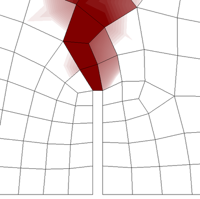
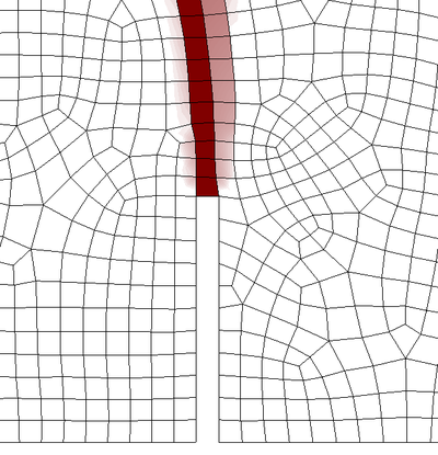
(a) Mesh 1.	(b) Mesh 3.
Figure 42: TPB test. Zoom of damage growing in the local model.

On the other side, in Figures 43a, 43b and 43c we see a very similar diffusive damaged area. Indeed, in the non-local approach, damage size is controlled by the interaction radius ${\textstyle R}$ and thus, even when reducing the size of the elements, the damaged area is practically unaltered.

(a) Mesh 1.

(b) Mesh 2.

(c) Mesh 3.

Figure 43: TPB test. Damage initiation in the non-local model.

This concept of damage localization and diffusion can also be seen in the evolution of damage obtained from the results of mesh 3 (Figure 44).

(a) Local model. Initial stage.	(b) Non-local model. Initial stage.
(c) Local model. Intermediate stage.	(d) Non-local model. Intermediate stage.
(e) Local model. Advanced stage.	(f) Non-local model. Advanced stage.
Figure 44: TPB test. Evolution of damage propagation.

The mesh-induced directional bias and mesh sensitivity observed in the local damage model are practically absent in the non-local model, and so the latter seems to be a more robust approach. However, apart from the mesh objectivity, it is important to assess whether the implemented model can properly reproduce the behaviour of the real beam. In this regard, we have compared the results obtained in the non-local model with experiments performed in [62].

Thereby, Figure 45 shows the force-vertical deflection diagram of the reference solution and the computed solution with mesh 3.

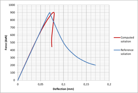
Figure 45: TPB test. Non-local model validation.

As we can see, the peak load is properly captured, but the post peak branch of the numerical solution falls faster than in the reference solution, and even shows a certain amount of snap-back behaviour. Moreover, looking at the elastic branch of the responses, it seems that the stiffness degradation starts before in the computed solution and, in consequence, the peak is slightly displaced to the right. Therefore, we can say that the behaviour of the numerical model seems more brittle than the observed in experiments.

4.2.2 Mesh-adaptive example

Finally, we are going to solve the same problem as before with the non-local damage model, but this time we will apply the implemented mesh-adaptive technique.

As we have commented, this adaptive procedure is a recent implementation still under development. As such, there are certain tools that are not currently available, but that need to be considered in the future. One of them is the possibility of measuring forces and displacements at points of interest in an adaptive mesh. Indeed, every time mesh is refined, nodes and elements numbering is altered, and so we cannot measure the forces and displacement like we did in the previous cases with a fixed mesh. Another limitation is that the current adaptive procedure has not any global indicator to initiate an error estimation and subsequent mesh refinement. This means that, before the problem starts, we must impose a certain number of refinements that will be performed uniformly distributed throughout all the incremental-iterative process.

Taking this into account, the main purpose of this subsection is simply to review an example of an adaptive procedure so as to understand the advantages and disadvantages of using this technique instead of a fixed mesh like before.

As commented in section 3.5, we will be using a remeshing criterion based on global error equidistribution. Moreover, we have considered a permissible percentage of global error of ${\textstyle \eta =10\%}$, we have imposed three refinements, and the initial mesh is a uniform unstructured mesh of quadrilaterals with an average size of 10 mm. The resulting spatial discretizations throughout the process are represented in Figure 46.

(a) Mesh 0: 4453 elements, 4618 nodes.	(b) Mesh 1: 2977 elements, 3146 nodes.
(c) Mesh 2: 1598 elements, 1731 nodes.	(d) Mesh 3: 1627 elements, 1759 nodes.
Figure 46: TPB test. Evolution of the adaptive mesh.

In order to understand the adaptive mesh process, it is interesting to see the evolution of damage for the different spatial discretizations (Figure 47), as well as the evolution of the refinement parameter of the elements ${\textstyle \xi ^{(e)}}$ (Figure 48).

(a) Mesh 0.

(b) Mesh 1.

(c) Mesh 2.

(d) Mesh 3.

Figure 47: TPB test. Progression of damage in the adaptive mesh.

Let us remember that the adaptive procedure estimates the error of the mesh from the effective stresses in the structure. Thereby, the parts of the structure with higher stress variations will tend to be refined, whereas those zones with smoother stresses will tend to have larger elements. This explains the concentration of elements at the zone of damage progression (Figure 47) and at the points of support and load application. Furthermore, the refinement parameter shown in Figure 48 represents the ratio between the actual element error and the desired error. Thereby, those elements depicted in blue (${\textstyle \xi ^{(e)}<1}$) are elements that could be larger, while the elements in red (${\textstyle \xi ^{(e)}>1}$) should be refined in order to reduce its error. Elements in green (${\textstyle \xi ^{(e)}=1}$) would be of optimal size.

(a) Mesh 0.

(b) Mesh 1.

(c) Mesh 2.

(d) Mesh 3.

Figure 48: TPB test. Progression of the refinement parameter in the adaptive mesh.

Looking at the number of elements in Figure 46, we can say that the main advantage of an adaptive mesh technique is that it automatically optimizes the mesh for the problem we are solving, so that the number of elements can be drastically reduced, and so the computational cost of the problem.

Nevertheless, this procedure has also shown some inconveniences when solving damage problems with a non-local approach. For instance, if damage starts propagating abruptly, the refinement process can lead to a considerable large amount of elements in the the damage zone. This concentration of elements can noticeably increase the cost of the non-local interactions and so the computation can become very intensive. However, the good point is that once damage propagation stabilizes, the adaptive procedure readjusts automatically the mesh, and so one ends with an actually efficient spatial discretization.

An additional limitation is that the procedure does not differentiate compressive stresses from tensile stresses when estimating the error. For materials like concrete this can lead to excessively small elements in compressed zones, and so it could be convenient to give a heavier weight to the tensile stresses.

Finally, one should also notice that the adaptive mesh process will always have some error associated to the transfer of internal variables between meshes. Thereby, once we can measure forces and displacements in adaptive mesh, we should check whether the response obtained with a fixed mesh is reproduced accurately in an adaptive process.

4.3 Single-Edge Notched Beam Test

In this second example a single-edge notched beam (SENB) is subjected to non-symmetrical four-point bending. The analysed beam has a square cross section of 100 ${\textstyle \times }$ 200 mm, a span of 840 mm, and the notch is 10 mm thick and 40 mm depth (see Figure 49).

Figure 49: SENB test. Problem statement. Distances in mm

Like in the previous case, in order to reduce fictitious stress concentrations at the supports and at the loading point, both the displacement constraints and the loads are acting over a line of 20 mm (see Figure 50).

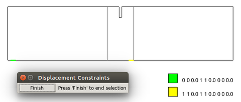
(a) Displacement constraints.

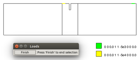
(b) Loads.

Figure 50: SENB test. Boundary Conditions.

Once again, we have assumed plane stress conditions, but in this case the geometry will be meshed by means of linear three-node triangular elements with 1 integration point.

4.3.1 Damage models testing

As we did for the three-point bending test, we will first solve the problem using the two implemented damage models. The local approach will be modelled with the same modified Simo and Ju model of the previous example, using the material parameters shown in Table 7. On the other hand, in this example the non-local damage model will be defined with the equivalent strain form of the modified von Mises model (26), and with the exponential damage evolution law that we presented in (36). The material parameters for the non-local approach have been obtained from [63], and are summarized in Table 8.

Table. 7 SENB test. Material parameters for the Simo-Ju local model.

Parameter	Value
Young's modulus (${\textstyle E}$)	28000 MPa
Poisson's ratio (${\textstyle \nu }$)	0.1
Compressive strength (${\textstyle \sigma _{y}^{c}}$)	35 MPa
Tensile strength (${\textstyle \sigma _{y}^{t}}$)	3.2 MPa
Fracture energy (${\textstyle G_{f}}$)	140 ${\textstyle J/m^{2}}$
Limit fracture length (${\textstyle l_{lim}}$)	5 mm

Table. 8 SENB test. Material parameters for the modified von Mises non-local model.

Parameter	Value
Young's modulus (${\textstyle E}$)	28000 MPa
Poisson's ratio (${\textstyle \nu }$)	0.1
Damage threshold (${\textstyle r_{0}}$)	${\textstyle 1.5\cdot {10}^{-4}}$
Compressive to tensile strength ratio (${\textstyle \kappa }$)	10
Parameter ${\textstyle A}$ (${\textstyle A}$)	0.8
Parameter ${\textstyle B}$ (${\textstyle B}$)	9000
Characteristic length (${\textstyle l_{c}}$)	10 mm

Just like before, we are going to solve the problem for different spatial discretizations. Thereby, we will be using three unstructured meshes of triangles with a minimum size of 8 mm, 5 mm, and 3 mm, respectively (see Figure 51).

(a) Mesh 1: 2216 elements, 1264 nodes.	(b) Mesh 2: 3502 elements, 1923 nodes.
(c) Mesh 3: 7183 elements, 3796 nodes.
Figure 51: SENB test. Spatial discretizations.

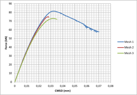
(a) Partially regularized local damage model.

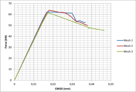
(b) Non-local damage model.

Figure 52: SENB test. Force-Crack Mouth Sliding Displacement curves.

Figure 52 shows the relation between the applied load and the Crack Mouth Sliding Displacement (CMSD). If we look at the curves in Figure 52a we can see that in this case the peak and the dissipated energy also decrease as the mesh is refinement. However, this reduction is not so clear as in the previous example. On the other hand, the response diagram in Figure 52b shows a peak load practically identical for the three meshes, but there are some differences in the response near the post-peak region.

Thereby, the response diagrams of the single-edge notched beam test seem to be in agreement with the ones obtained for the three-point bending test, although in this case the difference between the local and non-local approaches is not so clear. Now, in order to properly analyse the behaviour of both models, let us present some snapshots with the damage distribution.

Figures 53 and 54 show the damage progression in the peak region of the response, for the local and non-local model, respectively. Like before, from the size and shape of the damaged zone, we can clearly see a more localized response in the local damage model, and a more diffusive response in the non-local case.

Looking at the different damage patterns of the local model (Figure 53), we notice an additional vertical damage line that appears in the coarser meshes, stressing the idea that the local model suffers from mesh sensitivity.

(a) Mesh 1.

(b) Mesh 2.

(c) Mesh 3.

Figure 53: SENB test. Damage progression in the local model.

Regarding the non-local model (Figure 54), if we compare this example with the three-point bending test, we can clearly see that the progression zone here is restricted to a narrower region than before. The reason is that now the characteristic length defining the interaction radius is quite smaller than before.

(a) Mesh 1.

(b) Mesh 2.

(c) Mesh 3.

Figure 54: SENB test. Damage progression in the non-local model.

Focusing on the results obtained with mesh 3, the comparative evolution of damage for both models is represented in Figure 55.

(a) Local model. Initial stage.	(b) Non-local model. Initial stage.
(c) Local model. Intermediate stage.	(d) Non-local model. Intermediate stage.
(e) Local model. Advanced stage.	(f) Non-local model. Advanced stage.
Figure 55: SENB test. Evolution of damage propagation.

We can see that, at the beginning of damage propagation (Figures 55a and 55b) both approaches show a very similar damage zone. This more localized damage zone in the non-local model is mainly due to the reduced interaction radius of this example. After that, the difference between both models is noticeable.

Like in the previous case, we have compared the results obtained in the non-local model with an experimental solution [64].

Figure 56 shows the relation between the applied load and the Crack Mouth Sliding Displacement of the reference solution and the computed solution with mesh 3.

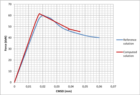
Figure 56: SENB test. Non-local model validation.

Thereby, we can see that the obtained response is very similar to the reference one. What we should notice, though, is that the failure obtained in the computed solution seems more brittle as compared to the reference one. This is possibly consequence of an imprecise tracing of the equilibrium path, caused by the global arc-length strategy used. As commented before, there are specific control parameters for the arc length method that are probably more suited for this kind of quasi-brittle behaviour.

4.3.2 Mesh-adaptive example

Finally, we are going to solve the problem again, applying the implemented mesh-adaptive technique on the non-local damage model.

Like in the three-point bending test, we will be using the remeshing criterion based on global error equidistribution, with a permissible percentage of global error of ${\textstyle \eta =10\%}$. In this case we have imposed four refinements, and the initial mesh is a uniform unstructured mesh of triangles with an average size of 7 mm. The resulting spatial discretizations throughout the process are represented in Figure 57.

(a) Mesh 0: 7784 elements, 4048 nodes.	(b) Mesh 1: 6800 elements, 3624 nodes.
(c) Mesh 2: 6590 elements, 3521 nodes.	(d) Mesh 3: 10626 elements, 5563 nodes.
(e) Mesh 4: 2542 elements, 1388 nodes.
Figure 57: SENB test. Evolution of the adaptive mesh.

Just like before, we are going to review the evolution of damage for the different spatial discretizations (Figure 58), as well as the evolution of the refinement parameter of the elements (Figure 59).

Looking at Figure 58a, we see that there is no damage in the original mesh. Moreover, if we look also at Figure 59a, it can be deduced that the subsequent spatial discretization is mainly caused by the high compressive stresses at the loading points and at the supports. Thereby, as we stated in the previous example, it could be very interesting to modify the evaluated stresses during the error estimation, in order to account for the different resistance in tension and compression of some geo-materials like concrete.

However, from Figures 57c, 57d and 57e it seems clear that the adaptive procedure properly captures the damage process zone and adapts the mesh accordingly.

(a) Mesh 0.

(b) Mesh 1.

(c) Mesh 2.

(d) Mesh 3.

(e) Mesh 4.

Figure 58: SENB test. Progression of damage in the adaptive mesh.

Another aspect to consider here is directly related to the abrupt failure of the computed solution seen in Figure 56. Indeed, as explained in the previous example, when damage grows abruptly, the adaptive technique refines excessively all the affected zone, as it can be seen from the predominant blue color in Figure 59d. Nonetheless, once damage stabilises the adaptive procedure readjusts the spatial discretization and the resulting mesh 57e is really efficient.

Finally, we can notice that the final damage pattern in Figure 58e is a bit wider than the one shown in 55f. The reason could be that some extra damage diffusion is introduced due to the errors appearing during the transfer of internal variables between meshes. Therefore, it would be interesting to obtain the force-CMSD curve when using this adaptive technique, in order to assess the effect of these errors in the traced equilibrium path.

(a) Mesh 0.

(b) Mesh 1.

(c) Mesh 2.

(d) Mesh 3.

(e) Mesh 4.

Figure 59: SENB test. Progression of the refinement parameter in the adaptive mesh.

5 Conclusions and Future Research Lines

We have been working in damage mechanics for almost half a year in the seek of a robust numerical method for the modelling of quasi-brittle materials failure, and we can point out the following conclusions.

First, we have seen that the partially regularization of the local damage model still shows mesh sensitiveness and presents severe mesh-induced directional bias, and so this model is not the best approach if one aims at achieving robust results. However, if the model is properly calibrated, it can become an interesting tool to obtain a first estimation of the damage propagation with a low computational cost.

On the other hand, the fully regularized non-local damage approach removes pathological mesh sensitivity and has proved to properly capture the peak load of the response diagrams in the three-point bending test, and in the single-edge notched beam test. In the former test, however, it has shown a more brittle post-peak branch as compared to the experimental results. Furthermore, an important aspect to note about this integral-type non-local approach is that the averaging performed to account for the non-local interaction, considerably increases the computational cost of the solution, as compared to the classical local approach, and also modifies the traditional assembly process of the global tangent stiffness matrix.

Concerning the non-linearity associated to damage, it must be stated that the implemented arc-length strategy has shown an irregular success when tracing the non-linear solution, and so it is probably not the best approach for the kind of problems we have been solving.

The implemented mesh-adaptive technique allows capturing the process damage zone and adjust the spatial discretization accordingly. This procedure generates large elements in zones with smooth stress distribution, and small elements in zones with strong variations of stresses, and so efficient mesh distributions can be obtained. However, the adaptive technique is still a recent implementation and there are some features that could be improved. For instance, the procedure does not differentiate compressive stresses from tensile stresses when estimating the error. This can lead to excessively fine meshes at compressed zones that are not actually transcendent for the damage progression of materials like concrete. Furthermore, errors in the transfer operations of internal variables introduce some extra damage diffusion that should be analysed in order to assess its influence in the traced equilibrium path.

Thereby, in the near future there are various aspects on the current code that should be enhanced. First, regarding the convergence of the non-linear solution, we could implement an advanced arc-length method with a specific control parameter (CMOD or CMSD) that accounts for the localized nature of quasi-brittle materials.

The measurement of forces and displacements in an adaptive mesh is also another important tool that would enable analysing the effect of the errors introduced into the response diagram of a structure, when transferring internal variables between different meshes.

Still in the mesh-adaptive technique, we could introduce some weights affecting the stresses evaluated in the error estimation process, in order to account for the different behaviour in tension and compression of many geo-materials. This way, even more optimized spatial discretizations could be generated, and the exaggerated concentrations of elements seen at the loading points and supports could be drastically reduced.

One last additional feature that should be implemented in the mesh-adaptive process, is a global error parameter that could be used to determine, at any load step, whether the error estimation process must be initialized or not.

Finally, as other research lines of interest, we should mention the extension of the implemented damage model and mesh-adaptive procedure to three-dimensional analysis; the coupling of damage and plasticity, necessary if one wants to simulate the interaction between concrete and steel; and the coupling of damage and fracture mechanics, which could make use of the information of the damage propagation to obtain the position and direction of an explicit fracture.

 

References

[1] Bazant, Zdenek P and Cedolin, Luigi. Blunt crack band propagation in finite element analysis, Volume 105. ASCE. Journal of the Engineering Mechanics Division 2 297–315, 1979

[2] Dragon, A and Mroz, Z. A continuum model for plastic-brittle behaviour of rock and concrete, Volume 17. Elsevier. International Journal of Engineering Science 2 121–137, 1979

[3] Di Prisco, M and Mazars, J. Crush-crack': a non-local damage model for concrete, Volume 1. Mechanics of Cohesive-frictional Materials 4 321–347, 1996

[4] Willam, KJ and Warnke, EP. Constitutive model for the triaxial behavior of concrete, Volume 19. ISMES, Bergamo, Italy 174, 1975

[5] De Borst, René. Non-linear analysis of frictional materials, 1986

[6] Lemaitre, Jean. Coupled elasto-plasticity and damage constitutive equations, Volume 51. Elsevier. Computer Methods in Applied Mechanics and Engineering 1 31–49, 1985

[7] Klisiski, M and Mroz, Z. Description of inelastic deformation and degradation of concrete, Volume 24. Elsevier. International journal of solids and structures 4 391–416, 1988

[8] Bazant, Zdenek P and Ozbolt, Josko. Nonlocal microplane model for fracture, damage, and size effect in structures, Volume 116. American Society of Civil Engineers. Journal of Engineering Mechanics 11 2485–2505, 1990

[9] Jirásek, Milan. Numerical modeling of deformation and failure of materials. Lecture notes, 1999

[10] Herrmann, HJ and Kertész, J and De Arcangelis, L. Fractal shapes of deterministic cracks, Volume 10. IOP Publishing. EPL (Europhysics Letters) 2 147, 1989

[11] Vervuurt, Adri and Van Mier, Jan GM and Schlangen, Erik. Analyses of anchor pull-out in concrete, Volume 27. Springer. Materials and Structures 5 251–259, 1994

[12] Sakaguchi, H and Mühlhaus, HB. Mesh free modelling of failure and localization in brittle materials. Pergamon: Oxford. Deformation and Progressive Failure in Geomechanics 15–21, 1997

[13] Recarey Morfa, Carlos A and Oñate, E and Rojek, Jerzy and Canet, Juan Miquel and Zarate, Francisco and Cadoce, Gilles and Labra, Carlos A. Modelación del ensayo Brasileño empleando modelación discreta. Ingeniería Civil 139, 2005

[14] Hult, J. Creep in continua and structures. Springer 137–155, 1974

[15] Kachanov, LM. On the time of fracture under conditions of creep. Izv. AN SSSR, Otd. Tekh. Nauk 8 26–35, 1958

[16] Rabotnov, YN. Damage from creep, Volume 2. Zhurn. Prikl. Mekh. Tekhn. Phys 113–123, 1963

[17] Hayhurst, DR. Creep rupture under multi-axial states of stress, Volume 20. Elsevier. Journal of the Mechanics and Physics of Solids 6 381–382, 1972

[18] Leckie, FA and Hayhurst, DR. Creep rupture of structures, Volume 340. The Royal Society. Proceedings of the Royal Society of London. A. Mathematical and Physical Sciences 1622 323–347, 1974

[19] Lemaitre, J and Chaboche, JL. Mécanique des matériaux solides, 1985. Dunod, Paris

[20] Mazars, Jacky. A description of micro-and macroscale damage of concrete structures, Volume 25. Elsevier. Engineering Fracture Mechanics 5 729–737, 1986

[21] Mazars, Jacky and Pijaudier-Cabot, Gilles. From damage to fracture mechanics and conversely: a combined approach, Volume 33. Elsevier. International Journal of Solids and Structures 20 3327–3342, 1996

[22] Chaboche, J-L. The concept of effective strain applied to elasticity and viscoelasticity in the presence of anisotropic damage 1979-77, 1979

[23] Simo, JC and Ju, JW. Strain-and stress-based continuum damage models-I. Formulation, Volume 23. Elsevier. International journal of solids and structures 7 821–840, 1987

[24] Ju, JW. Energy-based coupled elastoplastic damage models at finite strains, Volume 115. American Society of Civil Engineers. Journal of Engineering Mechanics 11 2507–2525, 1989

[25] Ju, JW. On energy-based coupled elastoplastic damage theories: constitutive modeling and computational aspects, Volume 25. Elsevier. International Journal of Solids and structures 7 803–833, 1989

[26] Oller, S and Oñate, E and Oliver, J and Lubliner, J. Finite element nonlinear analysis of concrete structures using a “plastic-damage model”, Volume 35. Elsevier. Engineering Fracture Mechanics 1 219–231, 1990

[27] Oliver, J and Cervera, M and Oller, S and Lubliner, J. Isotropic damage models and smeared crack analysis of concrete, Volume 2 945–958, 1990

[28] Oliver, J and Cervera, M and Oller, S and Lubliner, J. A simple damage model for concrete, including long term effects, Volume 2 945–958, 1990

[29] Cervera, M and Chiumenti, M and de Saracibar, C Agelet. Shear band localization via local J 2 continuum damage mechanics, Volume 193. Elsevier. Computer Methods in Applied Mechanics and Engineering 9 849–880, 2004

[30] Cervera, M and Chiumenti, M. Mesh objective tensile cracking via a local continuum damage model and a crack tracking technique, Volume 196. Elsevier. Computer Methods in Applied Mechanics and Engineering 1 304–320, 2006

[31] Mazars, Jacky. Application de la mécanique de l'endommagement au comportement non linéaire et a la rupture du béton de structure, 1984

[32] De Vree, JHP and Brekelmans, WAM and Van Gils, MAJ. Comparison of nonlocal approaches in continuum damage mechanics, Volume 55. Elsevier. Computers & Structures 4 581–588, 1995

[33] Pijaudier-Cabot, Gilles and Huerta, Antonio. Finite element analysis of bifurcation in nonlocal strain softening solids, Volume 90. Elsevier. Computer methods in applied mechanics and engineering 1 905–919, 1991

[34] Mühlhaus, HB. SHEARBAND ANALYSIS IN ANTIGRANULOCYTES MATERIAL BY COSSERAT-THEORY, Volume 56. SPRINGER VERLAG 175 FIFTH AVE, NEW YORK, NY 10010. Ingenieur Archiv 5 389–399, 1986

[35] Tejchman, J and Wu, W. Numerical study on patterning of shear bands in a Cosserat continuum, Volume 99. Springer. Acta Mechanica 1-4 61–74, 1993

[36] Zbib, HM and Aifantis, EC. A gradient-dependent flow theory of plasticity: application to metal and soil instabilities, Volume 42. American Society of Mechanical Engineers. Applied Mechanics Reviews 11S S295–S304, 1989

[37] Mühlhaus, HB and Alfantis, EC. A variational principle for gradient plasticity, Volume 28. Elsevier. International Journal of Solids and Structures 7 845–857, 1991

[38] Meftah, F and Reynouard, JM. A multilayered mixed beam element in gradient plasticity for the analysis of localized failure modes, Volume 3. Wiley Online Library. Mechanics of Cohesive-frictional Materials 4 305–322, 1998

[39] Loret, Benjamin and Prevost, Jean H. Dynamic strain localization in elasto-(visco-) plastic solids, Part 1. General formulation and one-dimensional examples, Volume 83. Elsevier. Computer Methods in Applied Mechanics and Engineering 3 247–273, 1990

[40] Prevost, Jean H and Loret, Benjamin. Dynamic strain localization in elasto-(visco-) plastic solids, part 2. Plane strain examples, Volume 83. Elsevier. Computer Methods in Applied Mechanics and Engineering 3 275–294, 1990

[41] Ehlers, W and Graf, T. Adaptive computation of localization phenomena in geotechnical applications. Bifurcations and Instabilities in Geomechanics, Swets, Zeitlinger 247–262, 2003

[42] Bazant, Zdeněk P. Mechanics of distributed cracking, Volume 39. American Society of Mechanical Engineers. Applied Mechanics Reviews 5 675–705, 1986

[43] Pijaudier-Cabot, Gilles and Bazant, Zdenek P. Nonlocal damage theory, Volume 113. American Society of Civil Engineers. Journal of Engineering Mechanics 10 1512–1533, 1987

[44] Jirásek, Milan and Rolshoven, Simon. Comparison of integral-type nonlocal plasticity models for strain-softening materials, Volume 41. Elsevier. International Journal of Engineering Science 13 1553–1602, 2003

[45] Rodríguez-Ferran, Antonio and Morata, Irene and Huerta, Antonio. A new damage model based on non-local displacements, Volume 29. Wiley Online Library. International Journal for Numerical and Analytical Methods in Geomechanics 5 473–493, 2005

[46] Bazant, Zdenek P and Oh, Byung H. Crack band theory for fracture of concrete, Volume 16. Springer. Matériaux et construction 3 155–177, 1983

[47] Pietruszczak, ST and Mroz, Z. Finite element analysis of deformation of strain-softening materials, Volume 17. Wiley Online Library. International Journal for Numerical Methods in Engineering 3 327–334, 1981

[48] Eringen, A Cemal. On nonlocal plasticity, Volume 19. Elsevier. International Journal of Engineering Science 12 1461–1474, 1981

[49] Eringen, A Cemal. On differential equations of nonlocal elasticity and solutions of screw dislocation and surface waves, Volume 54. AIP Publishing. Journal of Applied Physics 9 4703–4710, 1983

[50] Bazant, Zdenek P and Jirásek, Milan. Nonlocal integral formulations of plasticity and damage: survey of progress, Volume 128. American Society of Civil Engineers. Journal of Engineering Mechanics 11 1119–1149, 2002

[51] Timoshenko, S and Goodier, JN. Theory of elasticity, 1951, Volume 412. New York

[52] Crisfield, Michael A. Finite Elements and Solution Procedures for Structural Analysis V. 1: Linear Analysis, Volume 1. Pineridge Press Limited, 1986

[53] Oñate, Eugenio. Structural Analysis with the Finite Element Method. Linear Statics: Volume 1: Basis and Solids, Volume 1. Springer Science & Business Media, 2010

[54] Oñate, Eugenio. Structural Analysis with the Finite Element Method. Linear Statics: Volume 2: Beams, Plates and Shells, Volume 2. Springer Science & Business Media, 2013

[55] Ramm, Ekkehard. Strategies for tracing the nonlinear response near limit points. Springer, 1981

[56] Batoz, Jean-Louis and Dhatt, Gouri. Incremental displacement algorithms for nonlinear problems, Volume 14. Wiley Online Library. International Journal for Numerical Methods in Engineering 8 1262–1267, 1979

[57] Crisfield, Michael A. Non-linear finite element analysis of solids and structures: Advanced topics. John Wiley & Sons, Inc., 1997

[58] Portabella Castany, Miquel. Un procedimiento para cálculo de estructuras por el método de elementos finitos con error prefijado utilizando refinamiento de malla adaptativa. Universitat Politecnica de Catalunya, 2014

[59] Oñate, Eugenio. Cálculo de estructuras por el método de elementos finitos: análisis elástico lineal. Centro Internacional de Métodos Numéricos en Ingeniería, 1992

[60] Bugeda, G and Oñate, E. Adaptive mesh refinement techniques for aerodynamic problems. 513–522, 1992

[61] Oñate, Eugenio and Bugeda, Gabriel. A study of mesh optimality criteria in adaptive finite element analysis, Volume 10. MCB UP Ltd. Engineering computations 4 307–321, 1993

[62] Le Bellego, Caroline and normale supérieure de Cachan, École. Couplages chimie-mécanique dans les structures en béton attaquées par l'eau: Etude expérimentale et analyse numérique. LMT-ENS Cachan, 2001

[63] Rodríguez Ferran, Antonio and Arbós, Ivan and Huerta, Antonio and others. Adaptive analysis based on error estimation for nonlocal damage models, 2001

[64] Carpinteri, Alberto and Valente, Silvio and Ferrara, G and Melchiorrl, G. Is mode II fracture energy a real material property?, Volume 48. Elsevier. Computers & structures 3 397–413, 1993