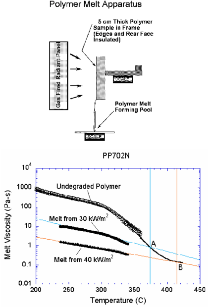
| Line 1: | Line 1: | ||
| + | <!-- metadata commented in wiki content | ||
==Possibilities of the particle finite element method in computational mechanics== | ==Possibilities of the particle finite element method in computational mechanics== | ||
| − | ''' | + | '''Eugenio Oñate, Sergio R. Idelsohn<math>^*</math>, Miguel Angel Celigueta, |
| − | + | Riccardo Rossi and Salvador Latorre''' | |
| − | + | ||
| − | < | + | {| |
| + | |- | ||
| + | |International Center for Numerical Methods in Engineering (CIMNE) | ||
| + | |- | ||
| + | | Technical University of Catalonia | ||
| + | |- | ||
| + | | Campus Norte UPC, 08034 Barcelona, Spain | ||
| + | |- | ||
| + | | [mailto:onate@cimne.upc.edu onate@cimne.upc.edu] | ||
| + | |- | ||
| + | | [http://www.cimne.com www.cimne.com] | ||
| + | |- | ||
| + | | <math>^*</math> ICREA Research Professor at CIMNE | ||
| + | |} | ||
| + | --> | ||
==Abstract== | ==Abstract== | ||
We present some developments in the formulation of the Particle Finite Element Method (PFEM) for analysis of complex coupled problems in fluid and solid mechanics accounting for fluid-structure interaction and coupled thermal effects. The PFEM uses an updated Lagrangian description to model the motion of nodes (particles) in both the fluid and the structure domains. Nodes are viewed as material points which can freely move and even separate from the main analysis domain representing, for instance, the effect of water drops. A mesh connects the nodes defining the discretized domain where the governing equations are solved as in the standard FEM. The necessary stabilization for dealing with the incompressibility of the fluid is introduced via the finite calculus (FIC) method. An incremental iterative scheme for the solution of the non linear transient coupled fluid-structure problem is described. Extensions of the PFEM to allow for frictional contact conditions at fluid-solid and solid-solid interfaces via mesh generation are described. A simple algorithm to treat erosion in the fluid bed is presented. Examples of application of the PFEM to solve a number of coupled problems such as the effect of large wave on structures, the large motions of floating and submerged bodies, bed erosion situations and melting and dripping of polymers under the effect of fire are given. | We present some developments in the formulation of the Particle Finite Element Method (PFEM) for analysis of complex coupled problems in fluid and solid mechanics accounting for fluid-structure interaction and coupled thermal effects. The PFEM uses an updated Lagrangian description to model the motion of nodes (particles) in both the fluid and the structure domains. Nodes are viewed as material points which can freely move and even separate from the main analysis domain representing, for instance, the effect of water drops. A mesh connects the nodes defining the discretized domain where the governing equations are solved as in the standard FEM. The necessary stabilization for dealing with the incompressibility of the fluid is introduced via the finite calculus (FIC) method. An incremental iterative scheme for the solution of the non linear transient coupled fluid-structure problem is described. Extensions of the PFEM to allow for frictional contact conditions at fluid-solid and solid-solid interfaces via mesh generation are described. A simple algorithm to treat erosion in the fluid bed is presented. Examples of application of the PFEM to solve a number of coupled problems such as the effect of large wave on structures, the large motions of floating and submerged bodies, bed erosion situations and melting and dripping of polymers under the effect of fire are given. | ||
| + | |||
| + | '''keywords''' | ||
==1 Introduction== | ==1 Introduction== | ||
| Line 37: | Line 54: | ||
The quality of the numerical solution depends on the discretization chosen as in the standard FEM. Adaptive mesh refinement techniques can be used to improve the solution in zones where large motions of the fluid or the structure occur. | The quality of the numerical solution depends on the discretization chosen as in the standard FEM. Adaptive mesh refinement techniques can be used to improve the solution in zones where large motions of the fluid or the structure occur. | ||
| − | {| style="text-align: center; border: 1px solid #BBB; margin: 1em auto; width: 100%;max-width: 100%;" | + | <div id='img-1'></div> |
| + | {| class="floating_imageSCP" style="text-align: center; border: 1px solid #BBB; margin: 1em auto; width: 100%;max-width: 100%;" | ||
|- | |- | ||
| − | |[[Image:draft_Samper_283227388-Figure1.png| | + | |[[Image:draft_Samper_283227388-Figure1.png|600px|Updated lagrangian description for a continuum containing a fluid and a solid domain]] |
|- style="text-align: center; font-size: 75%;" | |- style="text-align: center; font-size: 75%;" | ||
| − | | colspan="1" | '''Figure 1''' | + | | colspan="1" | '''Figure 1:''' Updated lagrangian description for a continuum containing a fluid and a solid domain |
|} | |} | ||
| − | {| style="text-align: center; border: 1px solid #BBB; margin: 1em auto; width: 100%;max-width: 100%;" | + | <div id='img-2'></div> |
| + | {| class="floating_imageSCP" style="text-align: center; border: 1px solid #BBB; margin: 1em auto; width: 100%;max-width: 100%;" | ||
|- | |- | ||
|[[Image:draft_Samper_283227388-Figure2.png|600px|Sequence of steps to update a “cloud” of nodes representing a domain containing a fluid and a solid part from time n (t=tₙ) to time n+2 (t=tₙ+2∆t) ]] | |[[Image:draft_Samper_283227388-Figure2.png|600px|Sequence of steps to update a “cloud” of nodes representing a domain containing a fluid and a solid part from time n (t=tₙ) to time n+2 (t=tₙ+2∆t) ]] | ||
|- style="text-align: center; font-size: 75%;" | |- style="text-align: center; font-size: 75%;" | ||
| − | | colspan="1" | '''Figure 2''' | + | | colspan="1" | '''Figure 2:''' Sequence of steps to update a “cloud” of nodes representing a domain containing a fluid and a solid part from time <math>n</math> (<math>t=t_n</math>) to time <math>n+2</math> (<math>t=t_n +2\Delta t</math>) |
|} | |} | ||
| Line 76: | Line 95: | ||
<div id='img-3'></div> | <div id='img-3'></div> | ||
| − | {| style="text-align: center; border: 1px solid #BBB; margin: 1em auto; width: 100%;max-width: 100%;" | + | {| class="floating_imageSCP" style="text-align: center; border: 1px solid #BBB; margin: 1em auto; width: 100%;max-width: 100%;" |
|- | |- | ||
|[[Image:draft_Samper_283227388-Cloud_nodes.png|600px|Sequence of steps to update in time a “cloud” of nodes representing a polymer object under thermal loads represented by a prescribed boundary heat flux q using the PFEM. Crossed circles denote prescribed nodes at the boundary ]] | |[[Image:draft_Samper_283227388-Cloud_nodes.png|600px|Sequence of steps to update in time a “cloud” of nodes representing a polymer object under thermal loads represented by a prescribed boundary heat flux q using the PFEM. Crossed circles denote prescribed nodes at the boundary ]] | ||
| Line 84: | Line 103: | ||
<div id='img-4'></div> | <div id='img-4'></div> | ||
| − | {| style="text-align: center; border: 1px solid #BBB; margin: 1em auto; width: 100%;max-width: 100%;" | + | {| class="floating_imageSCP" style="text-align: center; border: 1px solid #BBB; margin: 1em auto; width: 100%;max-width: 100%;" |
|- | |- | ||
|[[Image:draft_Samper_283227388-Figure2a_b.png|600px|]] | |[[Image:draft_Samper_283227388-Figure2a_b.png|600px|]] | ||
| − | + | |[[Image:draft_Samper_283227388-Fig2c.png|420px|Breakage of a water column. (a) Discretization of the fluid domain and the solid walls. Boundary nodes are marked with circles. (b) and (c) Mesh in the fluid domain at two different times]] | |
| − | |[[Image:draft_Samper_283227388-Fig2c.png| | + | |
|- style="text-align: center; font-size: 75%;" | |- style="text-align: center; font-size: 75%;" | ||
| − | | colspan=" | + | | colspan="2" | '''Figure 4:''' Breakage of a water column. (a) Discretization of the fluid domain and the solid walls. Boundary nodes are marked with circles. (b) and (c) Mesh in the fluid domain at two different times |
|} | |} | ||
| Line 107: | Line 125: | ||
|- | |- | ||
| | | | ||
| − | {| style="text-align: left; margin:auto;" | + | {| style="text-align: left; margin:auto;width: 100%;" |
|- | |- | ||
| style="text-align: center;" | <math>\rho {\partial v_i \over \partial t}={\partial \sigma _{ij} \over \partial x_j}+b_i\qquad \hbox{in } \Omega </math> | | style="text-align: center;" | <math>\rho {\partial v_i \over \partial t}={\partial \sigma _{ij} \over \partial x_j}+b_i\qquad \hbox{in } \Omega </math> | ||
|} | |} | ||
| − | | style="width: 5px;text-align: right;" | (1) | + | | style="width: 5px;text-align: right;white-space: nowrap;" | (1) |
|} | |} | ||
| Line 120: | Line 138: | ||
|- | |- | ||
| | | | ||
| − | {| style="text-align: left; margin:auto;" | + | {| style="text-align: left; margin:auto;width: 100%;" |
|- | |- | ||
| style="text-align: center;" | <math>{\partial v_i \over \partial x_i}=0 \qquad \hbox{in } \Omega </math> | | style="text-align: center;" | <math>{\partial v_i \over \partial x_i}=0 \qquad \hbox{in } \Omega </math> | ||
|} | |} | ||
| − | | style="width: 5px;text-align: right;" | (2) | + | | style="width: 5px;text-align: right;white-space: nowrap;" | (2) |
|} | |} | ||
| Line 133: | Line 151: | ||
|- | |- | ||
| | | | ||
| − | {| style="text-align: left; margin:auto;" | + | {| style="text-align: left; margin:auto;width: 100%;" |
|- | |- | ||
| style="text-align: center;" | <math>\rho c {\partial T \over \partial t}= {\partial \over \partial x_i} \left(k_i {\partial T \over \partial x_i}\right)+Q \qquad \hbox{in } \Omega </math> | | style="text-align: center;" | <math>\rho c {\partial T \over \partial t}= {\partial \over \partial x_i} \left(k_i {\partial T \over \partial x_i}\right)+Q \qquad \hbox{in } \Omega </math> | ||
|} | |} | ||
| − | | style="width: 5px;text-align: right;" | (3) | + | | style="width: 5px;text-align: right;white-space: nowrap;" | (3) |
|} | |} | ||
In above equations <math display="inline">v_{i}</math> is the velocity along the ''i''th global (cartesian) axis, <math display="inline">T</math> is the temperature, <math display="inline">\rho </math>, <math display="inline">c</math> and <math display="inline">k_i</math> are the density (assumed constant), the specific heat and the conductivity of the material along the ith coordinate direction, respectively, <math display="inline">b_i</math> and <math display="inline">Q</math> are the body forces and the heat source per unit mass, respectively and <math display="inline">\sigma _{ij}</math> are the (Cauchy) stresses related to the velocities by the standard constitutive equation (for incompressible Newtonian material) | In above equations <math display="inline">v_{i}</math> is the velocity along the ''i''th global (cartesian) axis, <math display="inline">T</math> is the temperature, <math display="inline">\rho </math>, <math display="inline">c</math> and <math display="inline">k_i</math> are the density (assumed constant), the specific heat and the conductivity of the material along the ith coordinate direction, respectively, <math display="inline">b_i</math> and <math display="inline">Q</math> are the body forces and the heat source per unit mass, respectively and <math display="inline">\sigma _{ij}</math> are the (Cauchy) stresses related to the velocities by the standard constitutive equation (for incompressible Newtonian material) | ||
| − | <span id="eq-4"></span> | + | <span id="eq-4.a"></span> |
{| class="formulaSCP" style="width: 100%; text-align: left;" | {| class="formulaSCP" style="width: 100%; text-align: left;" | ||
|- | |- | ||
| | | | ||
| − | {| style="text-align: left; margin:auto;" | + | {| style="text-align: left; margin:auto;width: 100%;" |
|- | |- | ||
| style="text-align: center;" | <math>\sigma _{ij} =s _{ij} - p \delta _{ij} </math> | | style="text-align: center;" | <math>\sigma _{ij} =s _{ij} - p \delta _{ij} </math> | ||
|} | |} | ||
| − | | style="width: 5px;text-align: right;" | (4) | + | | style="width: 5px;text-align: right;white-space: nowrap;" | (4.a) |
|} | |} | ||
| − | <span id="eq- | + | <span id="eq-4.b"></span> |
{| class="formulaSCP" style="width: 100%; text-align: left;" | {| class="formulaSCP" style="width: 100%; text-align: left;" | ||
|- | |- | ||
| | | | ||
| − | {| style="text-align: left; margin:auto;" | + | {| style="text-align: left; margin:auto;width: 100%;" |
|- | |- | ||
| style="text-align: center;" | <math>s _{ij}=2\mu \left(\dot \varepsilon _{ij}-\frac{1}{3}\delta _{ij}\dot \varepsilon _{ii} \right)\quad ,\quad \dot \varepsilon _{ij}=\frac{1}{2} \left({\partial v_i \over \partial x_j}+ {\partial v_j \over \partial x_i}\right) </math> | | style="text-align: center;" | <math>s _{ij}=2\mu \left(\dot \varepsilon _{ij}-\frac{1}{3}\delta _{ij}\dot \varepsilon _{ii} \right)\quad ,\quad \dot \varepsilon _{ij}=\frac{1}{2} \left({\partial v_i \over \partial x_j}+ {\partial v_j \over \partial x_i}\right) </math> | ||
|} | |} | ||
| − | | style="width: 5px;text-align: right;" | ( | + | | style="width: 5px;text-align: right;white-space: nowrap;" | (4.b) |
|} | |} | ||
| Line 170: | Line 188: | ||
Eqs.([[#eq-1|1]])–([[#3.1 Governing equations|3.1]]) are completed with the standard boundary conditions of prescribed velocities and surface tractions in the mechanical problem and prescribed temperature and prescribed normal heat flux in the thermal problem <span id='citeF-2'></span><span id='citeF-7'></span>[[#cite-2|[2,7]]]. | Eqs.([[#eq-1|1]])–([[#3.1 Governing equations|3.1]]) are completed with the standard boundary conditions of prescribed velocities and surface tractions in the mechanical problem and prescribed temperature and prescribed normal heat flux in the thermal problem <span id='citeF-2'></span><span id='citeF-7'></span>[[#cite-2|[2,7]]]. | ||
| − | We note that Eqs.([[#eq-1|1]])–([[#eq-3|3]]) are the standard ones for modeling the deformation of viscoplastic materials using the so called “flow approach” <span id='citeF-38'></span><span id='citeF-39'></span>[[#cite-38|[38,39]]]. In our work the dependence of the viscosity with the strain typical of viscoplastic flows has been simplified to the Newtonian form of Eq.([[#eq- | + | We note that Eqs.([[#eq-1|1]])–([[#eq-3|3]]) are the standard ones for modeling the deformation of viscoplastic materials using the so called “flow approach” <span id='citeF-38'></span><span id='citeF-39'></span>[[#cite-38|[38,39]]]. In our work the dependence of the viscosity with the strain typical of viscoplastic flows has been simplified to the Newtonian form of Eq.([[#eq-4.b|4.b]]). |
===3.2 Discretization of the equations=== | ===3.2 Discretization of the equations=== | ||
| Line 176: | Line 194: | ||
A key problem in the numerical solution of Eqs.([[#eq-1|1]])–([[#3.1 Governing equations|3.1]]) is the satisfaction of the incompressibility condition (Eq.([[#eq-2|2]])). A number of procedures to solve his problem exist in the finite element literature <span id='citeF-7'></span><span id='citeF-37'></span>[[#cite-7|[7,37]]]. In our approach we use a stabilized formulation based in the so-called finite calculus procedure <span id='citeF-19'></span>[[#cite-19|[19]]]–<span id='citeF-21'></span>[[#cite-21|[21]]],<span id='citeF-28'></span><span id='citeF-30'></span><span id='citeF-32'></span>[[#cite-28|[28,30,32]]]. The essence of this method is the solution of a ''modified mass balance'' equation which is written as | A key problem in the numerical solution of Eqs.([[#eq-1|1]])–([[#3.1 Governing equations|3.1]]) is the satisfaction of the incompressibility condition (Eq.([[#eq-2|2]])). A number of procedures to solve his problem exist in the finite element literature <span id='citeF-7'></span><span id='citeF-37'></span>[[#cite-7|[7,37]]]. In our approach we use a stabilized formulation based in the so-called finite calculus procedure <span id='citeF-19'></span>[[#cite-19|[19]]]–<span id='citeF-21'></span>[[#cite-21|[21]]],<span id='citeF-28'></span><span id='citeF-30'></span><span id='citeF-32'></span>[[#cite-28|[28,30,32]]]. The essence of this method is the solution of a ''modified mass balance'' equation which is written as | ||
| − | <span id="eq- | + | <span id="eq-5"></span> |
{| class="formulaSCP" style="width: 100%; text-align: left;" | {| class="formulaSCP" style="width: 100%; text-align: left;" | ||
|- | |- | ||
| | | | ||
| − | {| style="text-align: left; margin:auto;" | + | {| style="text-align: left; margin:auto;width: 100%;" |
|- | |- | ||
| style="text-align: center;" | <math>{\partial v_i \over \partial x_i}+\sum \limits _{i=1}^{3}\tau {\partial \over \partial x_i}\left[{\partial p \over \partial x_i} +\pi _i\right]=0 </math> | | style="text-align: center;" | <math>{\partial v_i \over \partial x_i}+\sum \limits _{i=1}^{3}\tau {\partial \over \partial x_i}\left[{\partial p \over \partial x_i} +\pi _i\right]=0 </math> | ||
|} | |} | ||
| − | | style="width: 5px;text-align: right;" | ( | + | | style="width: 5px;text-align: right;white-space: nowrap;" | (5) |
|} | |} | ||
where <math display="inline">\tau </math> is a stabilization parameter given by [10] | where <math display="inline">\tau </math> is a stabilization parameter given by [10] | ||
| − | <span id="eq- | + | <span id="eq-6"></span> |
{| class="formulaSCP" style="width: 100%; text-align: left;" | {| class="formulaSCP" style="width: 100%; text-align: left;" | ||
|- | |- | ||
| | | | ||
| − | {| style="text-align: left; margin:auto;" | + | {| style="text-align: left; margin:auto;width: 100%;" |
|- | |- | ||
| − | | style="text-align: center;" | <math>\tau = \left(\frac{2\rho \vert \ | + | | style="text-align: center;" | <math>\tau = \left(\frac{2\rho \vert \mathbf{v}\vert }{h}+\frac{8\mu }{3h^2} \right)^{-1} </math> |
|} | |} | ||
| − | | style="width: 5px;text-align: right;" | ( | + | | style="width: 5px;text-align: right;white-space: nowrap;" | (6) |
|} | |} | ||
| − | In the above, <math display="inline">h</math> is a characteristic length of each finite element (such as <math display="inline">[A^{(e)}]^{1/2}</math> for 2D elements) and <math display="inline">\vert \ | + | In the above, <math display="inline">h</math> is a characteristic length of each finite element (such as <math display="inline">[A^{(e)}]^{1/2}</math> for 2D elements) and <math display="inline">\vert \mathbf{v}\vert </math> is the modulus of the velocity vector. In Eq.([[#eq-5|5]]) <math display="inline">\pi _i</math> are auxiliary pressure projection variables chosen so as to ensure that the second term in Eq.([[#eq-5|5]]) can be interpreted as weighted sum of the residuals of the momentum equations and therefore it vanishes for the exact solution. The set of governing equations for the velocities, the pressure and the <math display="inline">\pi _i</math> variables is completed by adding the following constraint equation to the set of governing equations <span id='citeF-28'></span><span id='citeF-32'></span>[[#cite-28|[28,32]]] |
| − | <span id="eq- | + | <span id="eq-7"></span> |
{| class="formulaSCP" style="width: 100%; text-align: left;" | {| class="formulaSCP" style="width: 100%; text-align: left;" | ||
|- | |- | ||
| | | | ||
| − | {| style="text-align: left; margin:auto;" | + | {| style="text-align: left; margin:auto;width: 100%;" |
|- | |- | ||
| style="text-align: center;" | <math>\int _V \tau w_i\left({\partial p \over \partial x_i} +\pi _i\right)dV=0 \quad i=1,n_d </math> | | style="text-align: center;" | <math>\int _V \tau w_i\left({\partial p \over \partial x_i} +\pi _i\right)dV=0 \quad i=1,n_d </math> | ||
|} | |} | ||
| − | | style="width: 5px;text-align: right;" | ( | + | | style="width: 5px;text-align: right;white-space: nowrap;" | (7) |
|} | |} | ||
| Line 221: | Line 239: | ||
==Momentum== | ==Momentum== | ||
| − | <span id="eq- | + | <span id="eq-8"></span> |
{| class="formulaSCP" style="width: 100%; text-align: left;" | {| class="formulaSCP" style="width: 100%; text-align: left;" | ||
|- | |- | ||
| | | | ||
| − | {| style="text-align: left; margin:auto;" | + | {| style="text-align: left; margin:auto;width: 100%;" |
|- | |- | ||
| − | | style="text-align: center;" | <math>\ | + | | style="text-align: center;" | <math>\mathbf{M} \dot{\bar{v}} + \mathbf{K} (\mu )\bar {v} - \mathbf{G} \bar {p}= {f} </math> |
|} | |} | ||
| − | | style="width: 5px;text-align: right;" | ( | + | | style="width: 5px;text-align: right;white-space: nowrap;" | (8) |
|} | |} | ||
==Mass balance== | ==Mass balance== | ||
| − | <span id="eq- | + | <span id="eq-9"></span> |
{| class="formulaSCP" style="width: 100%; text-align: left;" | {| class="formulaSCP" style="width: 100%; text-align: left;" | ||
|- | |- | ||
| | | | ||
| − | {| style="text-align: left; margin:auto;" | + | {| style="text-align: left; margin:auto;width: 100%;" |
|- | |- | ||
| − | | style="text-align: center;" | <math>\ | + | | style="text-align: center;" | <math>\mathbf{G}\bar{v}+ \mathbf{L}\bar {p}+ \mathbf{Q} \bar {\boldsymbol \pi }=\mathbf{0} </math> |
|} | |} | ||
| − | | style="width: 5px;text-align: right;" | ( | + | | style="width: 5px;text-align: right;white-space: nowrap;" | (9) |
|} | |} | ||
==Pressure gradient projection== | ==Pressure gradient projection== | ||
| − | <span id="eq- | + | <span id="eq-10"></span> |
{| class="formulaSCP" style="width: 100%; text-align: left;" | {| class="formulaSCP" style="width: 100%; text-align: left;" | ||
|- | |- | ||
| | | | ||
| − | {| style="text-align: left; margin:auto;" | + | {| style="text-align: left; margin:auto;width: 100%;" |
|- | |- | ||
| − | | style="text-align: center;" | <math>\hat {M} \bar {\boldsymbol \pi }+\ | + | | style="text-align: center;" | <math>\hat {M} \bar {\boldsymbol \pi }+\mathbf{Q}^T\bar {p}=\mathbf{0} </math> |
|} | |} | ||
| − | | style="width: 5px;text-align: right;" | ( | + | | style="width: 5px;text-align: right;white-space: nowrap;" | (10) |
|} | |} | ||
==Heat transport== | ==Heat transport== | ||
| − | <span id="eq- | + | <span id="eq-11"></span> |
{| class="formulaSCP" style="width: 100%; text-align: left;" | {| class="formulaSCP" style="width: 100%; text-align: left;" | ||
|- | |- | ||
| | | | ||
| − | {| style="text-align: left; margin:auto;" | + | {| style="text-align: left; margin:auto;width: 100%;" |
|- | |- | ||
| − | | style="text-align: center;" | <math>\ | + | | style="text-align: center;" | <math>\mathbf{C}\dot{\bar{T}} + \mathbf{H} \bar {T} = {q} </math> |
|} | |} | ||
| − | | style="width: 5px;text-align: right;" | ( | + | | style="width: 5px;text-align: right;white-space: nowrap;" | (11) |
|} | |} | ||
| − | In Eqs.([[#eq- | + | In Eqs.([[#eq-8|8]])–([[#eq-11|11]]) <math display="inline">\bar{(\cdot )}</math> denotes nodal variables, <math display="inline">\dot{\bar{(\cdot )}}= {\partial \over \partial t}\bar{(\cdot )}</math>. The different matrices and vectors are given in the Appendix. |
| − | The solution in time of Eqs.([[#eq- | + | The solution in time of Eqs.([[#eq-8|8]])–([[#eq-11|11]]) can be performed using any time integration schemes typical of the updated Lagrangian finite element method. A basic algorithm following the conceptual process described in Section 2.1 is presented in Box I. <math display="inline">^{n+1}(\bar{a})^{j+1}</math> denotes the values of the nodal variables <math display="inline">\bar{a}</math> at time <math display="inline">n+1</math> and the <math display="inline">j+1</math> iterations. We note the coupling of the flow and thermal equations via the dependence of the viscosity <math display="inline">\mu </math> with the temperature. |
| − | {| style="text-align: center; border: 1px solid #BBB; margin: 1em auto; width: | + | {| class="floating_imageSCP" style="text-align: center; border: 1px solid #BBB; margin: 1em auto; width: 100%;max-width: 100%;" |
|- | |- | ||
|[[Image:draft_Samper_283227388-Box_I.png|480px|]] | |[[Image:draft_Samper_283227388-Box_I.png|480px|]] | ||
| Line 285: | Line 303: | ||
<div id='img-5'></div> | <div id='img-5'></div> | ||
| − | {| style="text-align: center; border: 1px solid #BBB; margin: 1em auto; width: 100%;max-width: 100%;" | + | {| class="floating_imageSCP" style="text-align: center; border: 1px solid #BBB; margin: 1em auto; width: 100%;max-width: 100%;" |
|- | |- | ||
| − | |[[Image:draft_Samper_283227388-Figure3a.png| | + | |[[Image:draft_Samper_283227388-Figure3a.png|450px|]] |
| − | |[[Image:draft_Samper_283227388-Figure3b.png| | + | |[[Image:draft_Samper_283227388-Figure3b.png|450px|Split of the analysis domain V into fluid and solid subdomains. Equality of surface tractions and kinematic variables at the common interface]] |
|- style="text-align: center; font-size: 75%;" | |- style="text-align: center; font-size: 75%;" | ||
| colspan="2" | '''Figure 5:''' Split of the analysis domain <math>V</math> into fluid and solid subdomains. Equality of surface tractions and kinematic variables at the common interface | | colspan="2" | '''Figure 5:''' Split of the analysis domain <math>V</math> into fluid and solid subdomains. Equality of surface tractions and kinematic variables at the common interface | ||
| Line 298: | Line 316: | ||
|- | |- | ||
| | | | ||
| − | {| style="text-align: left; margin:auto;" | + | {| style="text-align: left; margin:auto;width: 100%;" |
|- | |- | ||
| − | | style="text-align: | + | | style="text-align: center;" | <math>{}^t S := [{}^t {x}_s,{}^t {u}_s, {}^t {v}_s, {}^t {a}_s, {}^t {\boldsymbol \varepsilon }_s, {}^t {\boldsymbol \sigma }_s,{}^t {T}_s ]^T</math> |
| − | + | | style="width: 5px;text-align: right;white-space: nowrap;" | (12) | |
| − | + | ||
| − | | style="width: 5px;text-align: right;" | ( | + | |
|- | |- | ||
| − | | style="text-align: | + | | style="text-align: center;" | <math> {}^t F := [{}^t {x}_F,{}^t {u}_F, {}^t {v}_F, {}^t {a}_F, {}^t \dot{\boldsymbol \varepsilon }_F, {}^t {\boldsymbol \sigma }_F,{}^t {T}_F]^T </math> |
| − | + | | style="width: 5px;text-align: right;white-space: nowrap;" | (13) | |
| − | + | ||
| − | | style="width: 5px;text-align: right;" | ( | + | |
|} | |} | ||
|} | |} | ||
| Line 328: | Line 342: | ||
|- | |- | ||
| | | | ||
| − | {| style="text-align: left; margin:auto;" | + | {| style="text-align: left; margin:auto;width: 100%;" |
|- | |- | ||
| style="text-align: center;" | <math>{M}_s \bar {a}_s +{g}_s - {f}_s = {0} </math> | | style="text-align: center;" | <math>{M}_s \bar {a}_s +{g}_s - {f}_s = {0} </math> | ||
|} | |} | ||
| − | | style="width: 5px;text-align: right;" | ( | + | | style="width: 5px;text-align: right;white-space: nowrap;" | (14) |
|} | |} | ||
| Line 343: | Line 357: | ||
The above FSI solution algorithm is shown schematically in Box II. | The above FSI solution algorithm is shown schematically in Box II. | ||
| − | {| style="text-align: center; border: 1px solid #BBB; margin: 1em auto; width: | + | {| class="floating_imageSCP" style="text-align: center; border: 1px solid #BBB; margin: 1em auto; width: 100%;max-width: 100%;" |
|- | |- | ||
|[[Image:draft_Samper_283227388-Box_II.png|540px|]] | |[[Image:draft_Samper_283227388-Box_II.png|540px|]] | ||
| Line 353: | Line 367: | ||
<div id='img-6'></div> | <div id='img-6'></div> | ||
| − | {| style="text-align: center; border: 1px solid #BBB; margin: 1em auto; width: | + | {| class="floating_imageSCP" style="text-align: center; border: 1px solid #BBB; margin: 1em auto; width: 100%;max-width: 100%;" |
|- | |- | ||
|[[Image:draft_Samper_283227388-polygon.png|330px|Generation of non standard meshes combining different polygons (in 2D) and polyhedra (in 3D) using the extended Delaunay technique.]] | |[[Image:draft_Samper_283227388-polygon.png|330px|Generation of non standard meshes combining different polygons (in 2D) and polyhedra (in 3D) using the extended Delaunay technique.]] | ||
| Line 363: | Line 377: | ||
<div id='img-7'></div> | <div id='img-7'></div> | ||
| − | {| style="text-align: center; border: 1px solid #BBB; margin: 1em auto; width: | + | {| class="floating_imageSCP" style="text-align: center; border: 1px solid #BBB; margin: 1em auto; width: 100%;max-width: 100%;" |
|- | |- | ||
|[[Image:draft_Samper_283227388-etiquetas.png|540px|3D flow problem solved with the PFEM. CPU time for meshing, assembling and solving the system of equations at each time step in terms of the number of nodes]] | |[[Image:draft_Samper_283227388-etiquetas.png|540px|3D flow problem solved with the PFEM. CPU time for meshing, assembling and solving the system of equations at each time step in terms of the number of nodes]] | ||
| Line 377: | Line 391: | ||
<div id='img-8'></div> | <div id='img-8'></div> | ||
| − | {| style="text-align: center; border: 1px solid #BBB; margin: 1em auto; width: | + | {| class="floating_imageSCP" style="text-align: center; border: 1px solid #BBB; margin: 1em auto; width: 100%;max-width: 100%;" |
|- | |- | ||
|[[Image:draft_Samper_283227388-Identification.png|558px|Identification of individual particles (or a group of particles) starting from a given collection of nodes.]] | |[[Image:draft_Samper_283227388-Identification.png|558px|Identification of individual particles (or a group of particles) starting from a given collection of nodes.]] | ||
| Line 401: | Line 415: | ||
<div id='img-9'></div> | <div id='img-9'></div> | ||
| − | {| style="text-align: center; border: 1px solid #BBB; margin: 1em auto; width: 100%;max-width: 100%;" | + | {| class="floating_imageSCP" style="text-align: center; border: 1px solid #BBB; margin: 1em auto; width: 100%;max-width: 100%;" |
|- | |- | ||
| − | |[[Image:draft_Samper_283227388-Figure6_1.png| | + | |[[Image:draft_Samper_283227388-Figure6_1.png|570px|]] |
| − | |[[Image:draft_Samper_283227388-Figure8.png| | + | |[[Image:draft_Samper_283227388-Figure8.png|480px|Automatic treatment of contact conditions at the fluid-wall interface]] |
|- style="text-align: center; font-size: 75%;" | |- style="text-align: center; font-size: 75%;" | ||
| colspan="2" | '''Figure 9:''' Automatic treatment of contact conditions at the fluid-wall interface | | colspan="2" | '''Figure 9:''' Automatic treatment of contact conditions at the fluid-wall interface | ||
| Line 418: | Line 432: | ||
<div id='img-10'></div> | <div id='img-10'></div> | ||
| − | {| style="text-align: center; border: 1px solid #BBB; margin: 1em auto; width: 100%;max-width: 100%;" | + | {| class="floating_imageSCP" style="text-align: center; border: 1px solid #BBB; margin: 1em auto; width: 100%;max-width: 100%;" |
|- | |- | ||
|[[Image:draft_Samper_283227388-Contact_conditions.png|600px|Contact conditions at a solid-solid interface]] | |[[Image:draft_Samper_283227388-Contact_conditions.png|600px|Contact conditions at a solid-solid interface]] | ||
| Line 426: | Line 440: | ||
<div id='img-11'></div> | <div id='img-11'></div> | ||
| − | {| style="text-align: center; border: 1px solid #BBB; margin: 1em auto; width: 100%;max-width: 100%;" | + | {| class="floating_imageSCP" style="text-align: center; border: 1px solid #BBB; margin: 1em auto; width: 100%;max-width: 100%;" |
|- | |- | ||
| − | |[[Image:draft_Samper_283227388-bola.png| | + | |[[Image:draft_Samper_283227388-bola.png|410px|Bumping of a ball within a container. The layer of contact elements is shown at each contact instant]] |
|- style="text-align: center; font-size: 75%;" | |- style="text-align: center; font-size: 75%;" | ||
| colspan="1" | '''Figure 11:''' Bumping of a ball within a container. The layer of contact elements is shown at each contact instant | | colspan="1" | '''Figure 11:''' Bumping of a ball within a container. The layer of contact elements is shown at each contact instant | ||
| Line 434: | Line 448: | ||
<div id='img-12'></div> | <div id='img-12'></div> | ||
| − | {| style="text-align: center; border: 1px solid #BBB; margin: 1em auto; width: | + | {| class="floating_imageSCP" style="text-align: center; border: 1px solid #BBB; margin: 1em auto; width: 100%;max-width: 100%;" |
|- | |- | ||
| − | |[[Image:draft_Samper_283227388-arch.png| | + | |[[Image:draft_Samper_283227388-arch.png|351px|Failure of an arch formed by stone blocks under seismic loading]] |
|- style="text-align: center; font-size: 75%;" | |- style="text-align: center; font-size: 75%;" | ||
| colspan="1" | '''Figure 12:''' Failure of an arch formed by stone blocks under seismic loading | | colspan="1" | '''Figure 12:''' Failure of an arch formed by stone blocks under seismic loading | ||
| Line 442: | Line 456: | ||
<div id='img-13'></div> | <div id='img-13'></div> | ||
| − | {| style="text-align: center; border: 1px solid #BBB; margin: 1em auto; width: | + | {| class="floating_imageSCP" style="text-align: center; border: 1px solid #BBB; margin: 1em auto; width: 100%;max-width: 100%;" |
|- | |- | ||
| − | |[[Image:draft_Samper_283227388-tetrapods-six.png| | + | |[[Image:draft_Samper_283227388-tetrapods-six.png|336px|Motion of five tetrapods on an inclined plane]] |
|- style="text-align: center; font-size: 75%;" | |- style="text-align: center; font-size: 75%;" | ||
| colspan="1" | '''Figure 13:''' Motion of five tetrapods on an inclined plane | | colspan="1" | '''Figure 13:''' Motion of five tetrapods on an inclined plane | ||
| Line 464: | Line 478: | ||
|- | |- | ||
| | | | ||
| − | {| style="text-align: left; margin:auto;" | + | {| style="text-align: left; margin:auto;width: 100%;" |
|- | |- | ||
| − | | style="text-align: center;" | <math>\tau _t =\mu \gamma _t</math> | + | | style="text-align: center;" | <math> |
| + | |||
| + | \tau _t =\mu \gamma _t</li> | ||
| + | |||
| + | </math> | ||
| + | |} | ||
| + | | style="width: 5px;text-align: right;white-space: nowrap;" | (15.a) | ||
|} | |} | ||
| − | |||
| − | |||
with | with | ||
| Line 476: | Line 494: | ||
|- | |- | ||
| | | | ||
| − | {| style="text-align: left; margin:auto;" | + | {| style="text-align: left; margin:auto;width: 100%;" |
|- | |- | ||
| − | | style="text-align: center;" | <math>\gamma _t ={1\over 2}{\partial v_t\over \partial n} ={v_t^k\over 2h_k}</math> | + | | style="text-align: center;" | <math> |
| + | |||
| + | \gamma _t ={1\over 2}{\partial v_t\over \partial n} ={v_t^k\over 2h_k} | ||
| + | |||
| + | </math> | ||
|} | |} | ||
| − | | style="width: 5px;text-align: right;" | ( | + | | style="width: 5px;text-align: right;white-space: nowrap;" | (15.b) |
|} | |} | ||
| Line 490: | Line 512: | ||
|- | |- | ||
| | | | ||
| − | {| style="text-align: left; margin:auto;" | + | {| style="text-align: left; margin:auto;width: 100%;" |
|- | |- | ||
| − | | style="text-align: center;" | <math>W_f =\int _\circ ^t \tau _t \gamma _t\, dt = \int _\circ ^t {\mu \over 4} \left({v_t^k\over h_k}\right)^2 dt </math> | + | | style="text-align: center;" | <math> |
| + | |||
| + | W_f =\int _\circ ^t \tau _t \gamma _t\, dt = \int _\circ ^t {\mu \over 4} \left({v_t^k\over h_k}\right)^2 dt </li> | ||
| + | |||
| + | </math> | ||
| + | |} | ||
| + | | style="width: 5px;text-align: right;white-space: nowrap;" | (16) | ||
|} | |} | ||
| − | |||
| − | |||
Eq.(16) is integrated in time using a simple scheme as | Eq.(16) is integrated in time using a simple scheme as | ||
| Line 502: | Line 528: | ||
|- | |- | ||
| | | | ||
| − | {| style="text-align: left; margin:auto;" | + | {| style="text-align: left; margin:auto;width: 100%;" |
|- | |- | ||
| − | | style="text-align: center;" | <math>{}^n W_f ={}^{n-1} W_f + \tau _t \gamma _t\, \Delta t </math> | + | | style="text-align: center;" | <math> |
| + | |||
| + | {}^n W_f ={}^{n-1} W_f + \tau _t \gamma _t\, \Delta t | ||
| + | |||
| + | </math> | ||
|} | |} | ||
| − | | style="width: 5px;text-align: right;" | ( | + | | style="width: 5px;text-align: right;white-space: nowrap;" | (17) |
|} | |} | ||
| Line 514: | Line 544: | ||
<div id='img-14'></div> | <div id='img-14'></div> | ||
| − | {| style="text-align: center; border: 1px solid #BBB; margin: 1em auto; width: | + | {| class="floating_imageSCP" style="text-align: center; border: 1px solid #BBB; margin: 1em auto; width: 100%;max-width: 100%;" |
|- | |- | ||
|[[Image:draft_Samper_283227388-detail-tetrapods.png|540px|Detail of five tetrapods on an inclined plane. The layer of elements modeling the frictional contact conditions is shown]] | |[[Image:draft_Samper_283227388-detail-tetrapods.png|540px|Detail of five tetrapods on an inclined plane. The layer of elements modeling the frictional contact conditions is shown]] | ||
| Line 522: | Line 552: | ||
<div id='img-15'></div> | <div id='img-15'></div> | ||
| − | {| style="text-align: center; border: 1px solid #BBB; margin: 1em auto; width: 100%;max-width: 100%;" | + | {| class="floating_imageSCP" style="text-align: center; border: 1px solid #BBB; margin: 1em auto; width: 100%;max-width: 100%;" |
|- | |- | ||
|[[Image:draft_Samper_283227388-Erosion_fluid_forces.png|600px|Modeling of bed erosion by dragging of bed material]] | |[[Image:draft_Samper_283227388-Erosion_fluid_forces.png|600px|Modeling of bed erosion by dragging of bed material]] | ||
| Line 550: | Line 580: | ||
<div id='img-16'></div> | <div id='img-16'></div> | ||
| − | {| style="text-align: center; border: 1px solid #BBB; margin: 1em auto; width: 100%;max-width: 100%;" | + | {| class="floating_imageSCP" style="text-align: center; border: 1px solid #BBB; margin: 1em auto; width: 100%;max-width: 100%;" |
|- | |- | ||
| − | |[[Image:draft_Samper_283227388-fig16.png| | + | |[[Image:draft_Samper_283227388-fig16.png|870px|2D simulation of the penetration and evolution of a cube and a cylinder in a water container. The colours denote the different sizes of the elements at several times]] |
|- style="text-align: center; font-size: 75%;" | |- style="text-align: center; font-size: 75%;" | ||
| colspan="1" | '''Figure 16:''' 2D simulation of the penetration and evolution of a cube and a cylinder in a water container. The colours denote the different sizes of the elements at several times | | colspan="1" | '''Figure 16:''' 2D simulation of the penetration and evolution of a cube and a cylinder in a water container. The colours denote the different sizes of the elements at several times | ||
| Line 558: | Line 588: | ||
<div id='img-17'></div> | <div id='img-17'></div> | ||
| − | {| style="text-align: center; border: 1px solid #BBB; margin: 1em auto; width: 100%;max-width: 100%;" | + | {| class="floating_imageSCP" style="text-align: center; border: 1px solid #BBB; margin: 1em auto; width: 100%;max-width: 100%;" |
|- | |- | ||
| − | |[[Image:draft_Samper_283227388-Figure6.png|600px|Detail of element sizes during the motion of a rigid cylinder within | + | |[[Image:draft_Samper_283227388-Figure6.png|600px|Detail of element sizes during the motion of a rigid cylinder within a water container]] |
|- style="text-align: center; font-size: 75%;" | |- style="text-align: center; font-size: 75%;" | ||
| − | | colspan="1" | '''Figure 17:''' Detail of element sizes during the motion of a rigid cylinder within | + | | colspan="1" | '''Figure 17:''' Detail of element sizes during the motion of a rigid cylinder within a water container |
|} | |} | ||
<div id='img-18'></div> | <div id='img-18'></div> | ||
| − | {| style="text-align: center; border: 1px solid #BBB; margin: 1em auto; width: 100%;max-width: 100%;" | + | {| class="floating_imageSCP" style="text-align: center; border: 1px solid #BBB; margin: 1em auto; width: 100%;max-width: 100%;" |
|- | |- | ||
|[[Image:draft_Samper_283227388-diap9.png|600px|]] | |[[Image:draft_Samper_283227388-diap9.png|600px|]] | ||
| − | + | |[[Image:draft_Samper_283227388-diap10.png|600px|Evolution of a water column within a prismatic container including a vertical cylinder]] | |
| − | |[[Image:draft_Samper_283227388-diap10.png|600px|Evolution of a water column within a prismatic container including a | + | |
|- style="text-align: center; font-size: 75%;" | |- style="text-align: center; font-size: 75%;" | ||
| − | | colspan=" | + | | colspan="2" | '''Figure 18:''' Evolution of a water column within a prismatic container including a vertical cylinder |
|} | |} | ||
<div id='img-19'></div> | <div id='img-19'></div> | ||
| − | {| style="text-align: center; border: 1px solid #BBB; margin: 1em auto; width: 100%;max-width: 100%;" | + | {| class="floating_imageSCP" style="text-align: center; border: 1px solid #BBB; margin: 1em auto; width: 100%;max-width: 100%;" |
|- | |- | ||
| − | |[[Image:draft_Samper_283227388-diap17.png| | + | |[[Image:draft_Samper_283227388-diap17.png|555px|Impact of a wave on a prismatic column on a slab sustained by four pillars.]] |
|- style="text-align: center; font-size: 75%;" | |- style="text-align: center; font-size: 75%;" | ||
| − | | colspan="1" | '''Figure 19:''' Impact of a wave on a prismatic column on a slab sustained by four | + | | colspan="1" | '''Figure 19:''' Impact of a wave on a prismatic column on a slab sustained by four pillars. |
|} | |} | ||
<div id='img-20'></div> | <div id='img-20'></div> | ||
| − | {| style="text-align: center; border: 1px solid #BBB; margin: 1em auto; width: | + | {| class="floating_imageSCP" style="text-align: center; border: 1px solid #BBB; margin: 1em auto; width: 100%;max-width: 100%;" |
|- | |- | ||
|[[Image:draft_Samper_283227388-Figure11.png|570px|Dragging of a cubic object by a water stream.]] | |[[Image:draft_Samper_283227388-Figure11.png|570px|Dragging of a cubic object by a water stream.]] | ||
| Line 592: | Line 621: | ||
<div id='img-21'></div> | <div id='img-21'></div> | ||
| − | {| style="text-align: center; border: 1px solid #BBB; margin: 1em auto; width: 100%;max-width: 100%;" | + | {| class="floating_imageSCP" style="text-align: center; border: 1px solid #BBB; margin: 1em auto; width: 100%;max-width: 100%;" |
|- | |- | ||
|[[Image:draft_Samper_283227388-Fig15.png|600px|Interaction of a wave with a vertical pier formed by reinforced concrete cylinders.]] | |[[Image:draft_Samper_283227388-Fig15.png|600px|Interaction of a wave with a vertical pier formed by reinforced concrete cylinders.]] | ||
| Line 600: | Line 629: | ||
<div id='img-22'></div> | <div id='img-22'></div> | ||
| − | {| style="text-align: center; border: 1px solid #BBB; margin: 1em auto; width: 100%;max-width: 100%;" | + | {| class="floating_imageSCP" style="text-align: center; border: 1px solid #BBB; margin: 1em auto; width: 100%;max-width: 100%;" |
|- | |- | ||
|[[Image:draft_Samper_283227388-Fig16two.png|600px|Motion of two tetrapods falling in a water container.]] | |[[Image:draft_Samper_283227388-Fig16two.png|600px|Motion of two tetrapods falling in a water container.]] | ||
| Line 608: | Line 637: | ||
<div id='img-23'></div> | <div id='img-23'></div> | ||
| − | {| style="text-align: center; border: 1px solid #BBB; margin: 1em auto; width: 100%;max-width: 100%;" | + | {| class="floating_imageSCP" style="text-align: center; border: 1px solid #BBB; margin: 1em auto; width: 100%;max-width: 100%;" |
| − | + | ||
| − | + | ||
|- | |- | ||
| − | |[[Image:draft_Samper_283227388-diap26.png| | + | |[[Image:draft_Samper_283227388-diap25.png|535px|]] |
| + | |[[Image:draft_Samper_283227388-diap26.png|535px|Motion of ten tetrapods on a slope under an incident wave.]] | ||
|- style="text-align: center; font-size: 75%;" | |- style="text-align: center; font-size: 75%;" | ||
| − | | colspan=" | + | | colspan="2" | '''Figure 23:''' Motion of ten tetrapods on a slope under an incident wave. |
|} | |} | ||
<div id='img-24'></div> | <div id='img-24'></div> | ||
| − | {| style="text-align: center; border: 1px solid #BBB; margin: 1em auto; width: 100%;max-width: 100%;" | + | {| class="floating_imageSCP" style="text-align: center; border: 1px solid #BBB; margin: 1em auto; width: 100%;max-width: 100%;" |
|- | |- | ||
| − | |[[Image:draft_Samper_283227388-Figure24a.png| | + | |[[Image:draft_Samper_283227388-Figure24a.png|510px|]] |
| − | |[[Image:draft_Samper_283227388-Figure24b.png| | + | |[[Image:draft_Samper_283227388-Figure24b.png|510px|Detail of the motion of ten tetrapods on a slope under an incident wave. The figure shows the complex interactions between the water particles and the tetrapods.]] |
|- style="text-align: center; font-size: 75%;" | |- style="text-align: center; font-size: 75%;" | ||
| colspan="2" | '''Figure 24:''' Detail of the motion of ten tetrapods on a slope under an incident wave. The figure shows the complex interactions between the water particles and the tetrapods. | | colspan="2" | '''Figure 24:''' Detail of the motion of ten tetrapods on a slope under an incident wave. The figure shows the complex interactions between the water particles and the tetrapods. | ||
| Line 627: | Line 655: | ||
<div id='img-25'></div> | <div id='img-25'></div> | ||
| − | {| style="text-align: center; border: 1px solid #BBB; margin: 1em auto; width: | + | {| class="floating_imageSCP" style="text-align: center; border: 1px solid #BBB; margin: 1em auto; width: 100%;max-width: 100%;" |
|- | |- | ||
|[[Image:draft_Samper_283227388-Dique_bloques.png|420px|Effect of breaking waves on a breakwater slope containing reinforced concrete blocks. Detail of the mesh of 4-noded tetrahedra near the slope at two different times]] | |[[Image:draft_Samper_283227388-Dique_bloques.png|420px|Effect of breaking waves on a breakwater slope containing reinforced concrete blocks. Detail of the mesh of 4-noded tetrahedra near the slope at two different times]] | ||
| Line 663: | Line 691: | ||
<div id='img-26'></div> | <div id='img-26'></div> | ||
| − | {| style="text-align: center; border: 1px solid #BBB; margin: 1em auto; width: | + | {| class="floating_imageSCP" style="text-align: center; border: 1px solid #BBB; margin: 1em auto; width: 100%;max-width: 100%;" |
|- | |- | ||
|[[Image:draft_Samper_283227388-Dique_invernada.png|480px|Study of breaking waves on the edge of a breakwater structure formed by reinforced concrete blocks]] | |[[Image:draft_Samper_283227388-Dique_invernada.png|480px|Study of breaking waves on the edge of a breakwater structure formed by reinforced concrete blocks]] | ||
| Line 671: | Line 699: | ||
<div id='img-27'></div> | <div id='img-27'></div> | ||
| − | {| style="text-align: center; border: 1px solid #BBB; margin: 1em auto; width: 100%;max-width: 100%;" | + | {| class="floating_imageSCP" style="text-align: center; border: 1px solid #BBB; margin: 1em auto; width: 100%;max-width: 100%;" |
|- | |- | ||
| − | |[[Image:draft_Samper_283227388-camion.png| | + | |[[Image:draft_Samper_283227388-camion.png|481px|Effect of an overtopping wave on a truck passing by the perimetral road of a harbour adjacent to the breakwater]] |
|- style="text-align: center; font-size: 75%;" | |- style="text-align: center; font-size: 75%;" | ||
| colspan="1" | '''Figure 27:''' Effect of an overtopping wave on a truck passing by the perimetral road of a harbour adjacent to the breakwater | | colspan="1" | '''Figure 27:''' Effect of an overtopping wave on a truck passing by the perimetral road of a harbour adjacent to the breakwater | ||
| Line 679: | Line 707: | ||
<div id='img-28'></div> | <div id='img-28'></div> | ||
| − | {| style="text-align: center; border: 1px solid #BBB; margin: 1em auto; width: 100%;max-width: 100%;" | + | {| class="floating_imageSCP" style="text-align: center; border: 1px solid #BBB; margin: 1em auto; width: 100%;max-width: 100%;" |
|- | |- | ||
|[[Image:draft_Samper_283227388-erosion_3D.png|600px|Erosion of a 3D earth dam due to an overspill stream.]] | |[[Image:draft_Samper_283227388-erosion_3D.png|600px|Erosion of a 3D earth dam due to an overspill stream.]] | ||
| Line 695: | Line 723: | ||
<div id='img-29'></div> | <div id='img-29'></div> | ||
| − | {| style="text-align: center; border: 1px solid #BBB; margin: 1em auto; width: | + | {| class="floating_imageSCP" style="text-align: center; border: 1px solid #BBB; margin: 1em auto; width: 100%;max-width: 100%;" |
|- | |- | ||
|[[Image:draft_Samper_283227388-Fig3_polymers.png|420px|Polymer melt experiment. Viscosity vs. temperature for PP702N polypropylene in its initial undegraded form and after exposure to 30 kW/m² and 40 kW/m² heat fluxes. The black curve follows the extrapolation of viscosity to high temperatures.]] | |[[Image:draft_Samper_283227388-Fig3_polymers.png|420px|Polymer melt experiment. Viscosity vs. temperature for PP702N polypropylene in its initial undegraded form and after exposure to 30 kW/m² and 40 kW/m² heat fluxes. The black curve follows the extrapolation of viscosity to high temperatures.]] | ||
| Line 707: | Line 735: | ||
<div id='img-30'></div> | <div id='img-30'></div> | ||
| − | {| style="text-align: center; border: 1px solid #BBB; margin: 1em auto; width: 100%;max-width: 100%;" | + | {| class="floating_imageSCP" style="text-align: center; border: 1px solid #BBB; margin: 1em auto; width: 100%;max-width: 100%;" |
|- | |- | ||
| − | |[[Image:draft_Samper_283227388-Evolution_melt_1.png| | + | |[[Image:draft_Samper_283227388-Evolution_melt_1.png|600px|]] |
| − | |[[Image:draft_Samper_283227388-Evolution_melt_2.png| | + | |[[Image:draft_Samper_283227388-Evolution_melt_2.png|600px|]] |
|- | |- | ||
| − | |[[Image:draft_Samper_283227388-Evolution_melt_3.png| | + | |[[Image:draft_Samper_283227388-Evolution_melt_3.png|600px|]] |
| − | |[[Image:draft_Samper_283227388-Evolution_melt_4.png| | + | |[[Image:draft_Samper_283227388-Evolution_melt_4.png|600px|Evolution of the melt flow into the catch pan at t = 400s, 550s, 700s and 1000s]] |
|- style="text-align: center; font-size: 75%;" | |- style="text-align: center; font-size: 75%;" | ||
| colspan="2" | '''Figure 30:''' Evolution of the melt flow into the catch pan at t = 400s, 550s, 700s and 1000s | | colspan="2" | '''Figure 30:''' Evolution of the melt flow into the catch pan at t = 400s, 550s, 700s and 1000s | ||
| Line 725: | Line 753: | ||
<div id='img-31'></div> | <div id='img-31'></div> | ||
| − | {| style="text-align: center; border: 1px solid #BBB; margin: 1em auto; width: 100%;max-width: 100%;" | + | {| class="floating_imageSCP" style="text-align: center; border: 1px solid #BBB; margin: 1em auto; width: 100%;max-width: 100%;" |
|- | |- | ||
|[[Image:draft_Samper_283227388-Fig9_polymers.png|600px|Melt flow of a heated triangular object into a catch pan.]] | |[[Image:draft_Samper_283227388-Fig9_polymers.png|600px|Melt flow of a heated triangular object into a catch pan.]] | ||
| Line 733: | Line 761: | ||
<div id='img-32'></div> | <div id='img-32'></div> | ||
| − | {| style="text-align: center; border: 1px solid #BBB; margin: 1em auto; width: 100%;max-width: 100%;" | + | {| class="floating_imageSCP" style="text-align: center; border: 1px solid #BBB; margin: 1em auto; width: 100%;max-width: 100%;" |
|- | |- | ||
|[[Image:draft_Samper_283227388-Fig7_polymers.png|600px|Solution of a 3D polymer melt problem with the PFEM. Melt flow from a heated prismatic sample at different times.]] | |[[Image:draft_Samper_283227388-Fig7_polymers.png|600px|Solution of a 3D polymer melt problem with the PFEM. Melt flow from a heated prismatic sample at different times.]] | ||
| Line 877: | Line 905: | ||
|- | |- | ||
| | | | ||
| − | {| style="text-align: left; margin:auto;" | + | {| style="text-align: left; margin:auto;width: 100%;" |
|- | |- | ||
| − | | style="text-align: center;" | <math>\ | + | | style="text-align: center;" | <math>\mathbf{M}_{ij} =\int _{V^{e}} \rho \mathbf{N}_{i}^{T} \mathbf{N}_{j} dV \quad , \quad \mathbf{K}_{ij}=\int _{V^{e}} \mathbf{B}_{i}^{T} \mathbf{D} \mathbf{B}_{j} dV </math> |
|} | |} | ||
|} | |} | ||
| Line 886: | Line 914: | ||
|- | |- | ||
| | | | ||
| − | {| style="text-align: left; margin:auto;" | + | {| style="text-align: left; margin:auto;width: 100%;" |
|- | |- | ||
| − | | style="text-align: center;" | <math> \ | + | | style="text-align: center;" | <math> \mathbf{G}_{ij} = \int _{V^{e}} \mathbf{B}_{i}^{T} \mathbf{m}\mathbf{N}_{j} dV \quad , \quad \mathbf{f}_{i}=\int _{V^{e}} \mathbf{ N}_{i}^{T}\mathbf{b}dV+ \int _{\Gamma ^e} \mathbf{ N}_{i}^{T}\mathbf{t}d\Gamma </math> |
|} | |} | ||
|} | |} | ||
| Line 895: | Line 923: | ||
|- | |- | ||
| | | | ||
| − | {| style="text-align: left; margin:auto;" | + | {| style="text-align: left; margin:auto;width: 100%;" |
|- | |- | ||
| style="text-align: center;" | <math>{L}_{ij} = \int _{V^e} {\boldsymbol \nabla }^T N_i \tau {\boldsymbol \nabla }N_j dV \quad ,\quad {\boldsymbol \nabla } = \left[{\partial \over \partial x_1},{\partial \over \partial x_2},{\partial \over \partial x_3}\right]^T</math> | | style="text-align: center;" | <math>{L}_{ij} = \int _{V^e} {\boldsymbol \nabla }^T N_i \tau {\boldsymbol \nabla }N_j dV \quad ,\quad {\boldsymbol \nabla } = \left[{\partial \over \partial x_1},{\partial \over \partial x_2},{\partial \over \partial x_3}\right]^T</math> | ||
| Line 904: | Line 932: | ||
|- | |- | ||
| | | | ||
| − | {| style="text-align: left; margin:auto;" | + | {| style="text-align: left; margin:auto;width: 100%;" |
|- | |- | ||
| − | | style="text-align: center;" | <math>{Q}= [{Q}_1,{Q}_2,{Q}_3]\quad ,\quad [\ | + | | style="text-align: center;" | <math>{Q}= [{Q}_1,{Q}_2,{Q}_3]\quad ,\quad [\mathbf{Q}_{k}]_{ij} = \int _{V^e}\tau {\partial N_i \over \partial x_k} \mathbf{N}_j dV</math> |
|} | |} | ||
|} | |} | ||
| Line 913: | Line 941: | ||
|- | |- | ||
| | | | ||
| − | {| style="text-align: left; margin:auto;" | + | {| style="text-align: left; margin:auto;width: 100%;" |
|- | |- | ||
| style="text-align: center;" | <math>\hat {M}= \left[\hat {M}_1, \hat {M}_2,\hat {M}_3\right]\,,\, [\hat {M}_i]_{kl}=\left(\int _{V^e} \tau {N}_i{N}_j dV \right)\delta _{kl}\quad k,l=1,2,3</math> | | style="text-align: center;" | <math>\hat {M}= \left[\hat {M}_1, \hat {M}_2,\hat {M}_3\right]\,,\, [\hat {M}_i]_{kl}=\left(\int _{V^e} \tau {N}_i{N}_j dV \right)\delta _{kl}\quad k,l=1,2,3</math> | ||
| Line 922: | Line 950: | ||
|- | |- | ||
| | | | ||
| − | {| style="text-align: left; margin:auto;" | + | {| style="text-align: left; margin:auto;width: 100%;" |
|- | |- | ||
| style="text-align: center;" | <math>{B}=[{B}_1,{B}_2,{B}_3,{B}_4];\, {B}_i =\left[\begin{matrix} \displaystyle {\partial N_i \over \partial x}&0&0\\ 0 & \displaystyle {\partial N_i \over \partial y} &0\\ 0&0& \displaystyle {\partial N_i \over \partial z} \\ \displaystyle {\partial N_i \over \partial y} & \displaystyle {\partial N_i \over \partial x}&0\\\\ \displaystyle {\partial N_i \over \partial z} &0&\displaystyle {\partial N_i \over \partial x}\\\\ 0& \displaystyle {\partial N_i \over \partial z} &\displaystyle {\partial N_i \over \partial y} \end{matrix} \right]</math> | | style="text-align: center;" | <math>{B}=[{B}_1,{B}_2,{B}_3,{B}_4];\, {B}_i =\left[\begin{matrix} \displaystyle {\partial N_i \over \partial x}&0&0\\ 0 & \displaystyle {\partial N_i \over \partial y} &0\\ 0&0& \displaystyle {\partial N_i \over \partial z} \\ \displaystyle {\partial N_i \over \partial y} & \displaystyle {\partial N_i \over \partial x}&0\\\\ \displaystyle {\partial N_i \over \partial z} &0&\displaystyle {\partial N_i \over \partial x}\\\\ 0& \displaystyle {\partial N_i \over \partial z} &\displaystyle {\partial N_i \over \partial y} \end{matrix} \right]</math> | ||
| Line 931: | Line 959: | ||
|- | |- | ||
| | | | ||
| − | {| style="text-align: left; margin:auto;" | + | {| style="text-align: left; margin:auto;width: 100%;" |
|- | |- | ||
| style="text-align: center;" | <math>{D} =\mu \left[\begin{matrix}2 &0&0&0&0&0\\ 0&2&0&0&0&0\\ 0&0&2&0&0&0\\ 0&0&0&1&0&0\\ 0&0&0&0&1&0\\ 0&0&0&0&0&1\end{matrix}\right]</math> | | style="text-align: center;" | <math>{D} =\mu \left[\begin{matrix}2 &0&0&0&0&0\\ 0&2&0&0&0&0\\ 0&0&2&0&0&0\\ 0&0&0&1&0&0\\ 0&0&0&0&1&0\\ 0&0&0&0&0&1\end{matrix}\right]</math> | ||
| Line 940: | Line 968: | ||
|- | |- | ||
| | | | ||
| − | {| style="text-align: left; margin:auto;" | + | {| style="text-align: left; margin:auto;width: 100%;" |
|- | |- | ||
| style="text-align: center;" | <math>{N}=[{N}_1,{N}_2,{N}_3,{N}_4] \quad , \quad {N}_i={N}_i {I}_3\quad ,\quad {I}_3 \quad \hbox{is the unit matrix}</math> | | style="text-align: center;" | <math>{N}=[{N}_1,{N}_2,{N}_3,{N}_4] \quad , \quad {N}_i={N}_i {I}_3\quad ,\quad {I}_3 \quad \hbox{is the unit matrix}</math> | ||
| Line 949: | Line 977: | ||
|- | |- | ||
| | | | ||
| − | {| style="text-align: left; margin:auto;" | + | {| style="text-align: left; margin:auto;width: 100%;" |
|- | |- | ||
| style="text-align: center;" | <math>{C}_{ij}=\int _{V^e} \rho {c}{N}_i {N}_j dV \quad ,\quad {H}_{ij}= \int _{V^e}{\boldsymbol \nabla }^T {N}_i [k] {\boldsymbol \nabla }{N}_j dV \quad ,\quad {m} =[1,1,1,0,0,0]^T</math> | | style="text-align: center;" | <math>{C}_{ij}=\int _{V^e} \rho {c}{N}_i {N}_j dV \quad ,\quad {H}_{ij}= \int _{V^e}{\boldsymbol \nabla }^T {N}_i [k] {\boldsymbol \nabla }{N}_j dV \quad ,\quad {m} =[1,1,1,0,0,0]^T</math> | ||
| Line 958: | Line 986: | ||
|- | |- | ||
| | | | ||
| − | {| style="text-align: left; margin:auto;" | + | {| style="text-align: left; margin:auto;width: 100%;" |
|- | |- | ||
| style="text-align: center;" | <math>[k]= \left[\begin{matrix}k_1 &0 &0 \\ 0 & k_2&0\\ 0&0& k_3\end{matrix}\right]\quad , \quad q_i =\int _{V^e}N_iQdV - \int _{\Gamma _q^{e}} N_i q_n d\Gamma </math> | | style="text-align: center;" | <math>[k]= \left[\begin{matrix}k_1 &0 &0 \\ 0 & k_2&0\\ 0&0& k_3\end{matrix}\right]\quad , \quad q_i =\int _{V^e}N_iQdV - \int _{\Gamma _q^{e}} N_i q_n d\Gamma </math> | ||
| Line 964: | Line 992: | ||
|} | |} | ||
| − | In above equations indexes <math display="inline">i,j</math> run from 1 to the number of element nodes (4 for a tetrahedron), <math display="inline">q_n</math> is the heat flow prescribed at the external boundary <math display="inline">\Gamma _q</math>, '''t''' is the surface traction vector <math display="inline">\ | + | In above equations indexes <math display="inline">i,j</math> run from 1 to the number of element nodes (4 for a tetrahedron), <math display="inline">q_n</math> is the heat flow prescribed at the external boundary <math display="inline">\Gamma _q</math>, '''t''' is the surface traction vector <math display="inline">\mathbf{t}=[t_x,t_y,t_z]^T</math> and <math display="inline">V^{e}</math> and <math display="inline">\Gamma ^e</math> are the element volume and the element boundary, respectively. |
Revision as of 11:26, 13 March 2018
Abstract
We present some developments in the formulation of the Particle Finite Element Method (PFEM) for analysis of complex coupled problems in fluid and solid mechanics accounting for fluid-structure interaction and coupled thermal effects. The PFEM uses an updated Lagrangian description to model the motion of nodes (particles) in both the fluid and the structure domains. Nodes are viewed as material points which can freely move and even separate from the main analysis domain representing, for instance, the effect of water drops. A mesh connects the nodes defining the discretized domain where the governing equations are solved as in the standard FEM. The necessary stabilization for dealing with the incompressibility of the fluid is introduced via the finite calculus (FIC) method. An incremental iterative scheme for the solution of the non linear transient coupled fluid-structure problem is described. Extensions of the PFEM to allow for frictional contact conditions at fluid-solid and solid-solid interfaces via mesh generation are described. A simple algorithm to treat erosion in the fluid bed is presented. Examples of application of the PFEM to solve a number of coupled problems such as the effect of large wave on structures, the large motions of floating and submerged bodies, bed erosion situations and melting and dripping of polymers under the effect of fire are given.
keywords
1 Introduction
The analysis of problems involving the interaction of fluids and structures accounting for large motions of the fluid free surface and the existence of fully or partially submerged bodies which interact among themselves is of big relevance in many areas of engineering. Examples are common in ship hydrodynamics, off-shore and harbour structures, spill-ways in dams, free surface channel flows, environmental flows, liquid containers, stirring reactors, mould filling processes, etc.
Typical difficulties of fluid-multibody interaction analysis in free surface flows using the FEM with both the Eulerian and ALE formulation include the treatment of the convective terms and the incompressibility constraint in the fluid equations, the modelling and tracking of the free surface in the fluid, the transfer of information between the fluid and the moving solid domains via the contact interfaces, the modeling of wave splashing, the possibility to deal with large motions of the bodies within the fluid domain, the efficient updating of the finite element meshes for both the structure and the fluid, etc. For a comprehensive list of references in FEM for fluid flow problems see [7,37] and the references there included. A survey of recent works in fluid-structure interaction analysis can be found in [18], [27] and [35].
Most of the above problems disappear if a Lagrangian description is used to formulate the governing equations of both the solid and the fluid domains. In the Lagrangian formulation the motion of the individual particles are followed and, consequently, nodes in a finite element mesh can be viewed as moving material points (hereforth called “particles”). Hence, the motion of the mesh discretizing the total domain (including both the fluid and solid parts) is followed during the transient solution.
The authors have successfully developed in previous works a particular class of Lagrangian formulation for solving problems involving complex interaction between fluids and solids. The method, called the particle finite element method (PFEM, www.cimne.com/pfem), treats the mesh nodes in the fluid and solid domains as particles which can freely move and even separate from the main fluid domain representing, for instance, the effect of water drops. A mesh connects the nodes discretizing the domain where the governing equations are solved using a stabilized FEM.
The FEM solution of the variables in the (incompressible) fluid domain implies solving the momentum and incompressibility equations. This is not such as simple problem as the incompressibility condition limits the choice of the FE approximations for the velocity and pressure to overcome the well known -stability condition [7,37]. In our work we use a stabilized mixed FEM based on the Finite Calculus (FIC) approach which allows for a linear approximation for the velocity and pressure variables.
An advantage of the Lagrangian formulation is that the convective terms disappear from the fluid equations. The difficulty is however transferred to the problem of adequately (and efficiently) moving the mesh nodes. We use a mesh regeneration procedure blending elements of different shapes using an extended Delaunay tesselation with special shape functions [11,13]. The theory and applications of the PFEM are reported in [2,6,11,12,14,15,26,27,28,30,31,32].
The aim of this paper is to describe recent advances of the PFEM for a) the analysis of the interaction between a collection of bodies which are floating and/or submerged in the fluid, b) the modeling of bed erosion in open channel flows and c) the analysis of melting and dripping of polymer objects in fire situations. These problems are of great relevance in many areas of civil, marine and naval engineering, among others. It is shown that the PFEM provides a general analysis methodology for treat such a complex problems in a simple and efficient manner.
The layout of the paper is the following. In the next section the key ideas of the PFEM are outlined. Next the basic equations for an incompressible thermal flow using a Lagrangian description and the FIC formulation are presented. Then an algorithm for the transient solution is briefly described. The treatment of the coupled FSI problem and the methods for mesh generation and for identification of the free surface nodes are outlined. The procedure for treating at mesh generation level the contact conditions at fluid-wall interfaces and the frictional contact interaction between moving solids is explained. A methodology for modeling bed erosion due to fluid forces is described. Finally, the potencial of the PFEM is shown in its application to problems involving large flow motions, surface waves, moving bodies in water, bed erosion and melting and dripping of polymers in fire situations.
2 The basis of the particle finite element method
Let us consider a domain containing both fluid and solid subdomains. The moving fluid particles interact with the solid boundaries thereby inducing the deformation of the solid which in turn affects the flow motion and, therefore, the problem is fully coupled.
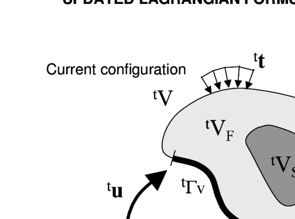
In the PFEM both the fluid and the solid domains are modelled using an updated Lagrangian formulation. That is, all variables in the fluid and solid domains are assumed to be known in the current configuration at time . The new set of variables in both domains are sought for in the next or updated configuration at time (Figure 1). The finite element method (FEM) is used to solve the continuum equations in both domains. Hence a mesh discretizing these domains must be generated in order to solve the governing equations for both the fluid and solid problems in the standard FEM fashion. Recall that the nodes discretizing the fluid and solid domains are treated as material particles which motion is tracked during the transient solution. This is useful to model the separation of fluid particles from the main fluid domain in a splashing wave, or soil particles in a bed erosion problem, and to follow their subsequent motion as individual particles with a known density, an initial acceleration and velocity and subject to gravity forces. The mass of a given domain is obtained by integrating the density at the different material points over the domain.
The quality of the numerical solution depends on the discretization chosen as in the standard FEM. Adaptive mesh refinement techniques can be used to improve the solution in zones where large motions of the fluid or the structure occur.
|
| Figure 1: Updated lagrangian description for a continuum containing a fluid and a solid domain |
|
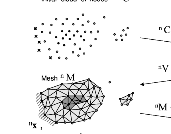
| Figure 2: Sequence of steps to update a “cloud” of nodes representing a domain containing a fluid and a solid part from time () to time () |
2.1 Basic steps of the PFEM
For clarity purposes we will define the collection or cloud of nodes (C) pertaining to the fluid and solid domains, the volume (V) defining the analysis domain for the fluid and the solid and the mesh (M) discretizing both domains.
A typical solution with the PFEM involves the following steps.
- The starting point at each time step is the cloud of points in the fluid and solid domains. For instance denotes the cloud at time (Figure 2).
- Identify the boundaries for both the fluid and solid domains defining the analysis domain in the fluid and the solid. This is an essential step as some boundaries (such as the free surface in fluids) may be severely distorted during the solution, including separation and re-entering of nodes. The Alpha Shape method [8] is used for the boundary definition (Section 5).
- Discretize the fluid and solid domains with a finite element mesh . In our work we use an innovative mesh generation scheme based on the extended Delaunay tesselation (Section 4) [11,12,14].
- Solve the coupled Lagrangian equations of motion for the fluid and the solid domains. Compute the state variables in both domains at the next (updated) configuration for : velocities, pressure, viscous stresses and temperature in the fluid and displacements, stresses, strains and temperature in the solid.
- Move the mesh nodes to a new position where denotes the time , in terms of the time increment size. This step is typically a consequence of the solution process of step 4.
- Go back to step 1 and repeat the solution process for the next time step to obtain . The process is shown in Figure 2.
Figure 3 shows another conceptual example of application of the PFEM to model the melting and dripping of a polymer object under a heat source acting at a boundary.

|
|
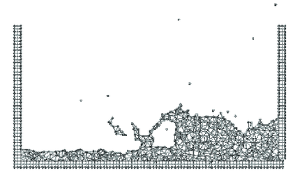
| Figure 4: Breakage of a water column. (a) Discretization of the fluid domain and the solid walls. Boundary nodes are marked with circles. (b) and (c) Mesh in the fluid domain at two different times | |
Figure 4 shows a typical example of a PFEM solution in 2D. The pictures correspond to the analysis of the problem of breakage of a water column [14,28]. Figure 4a shows the initial grid of four node rectangles discretizing the fluid domain and the solid walls. Figures 4b and 4c show the mesh for the solution at two later times.
3 FIC/FEM formulation for a lagrangian incompressible thermal fluid
3.1 Governing equations
The key equations to be solved in the incompressible thermal flow problem, written in the Lagrangian frame of reference, are the following:
Momentum
|
|
(1) |
Mass balance
|
|
(2) |
Heat transport
|
|
(3) |
In above equations is the velocity along the ith global (cartesian) axis, is the temperature, , and are the density (assumed constant), the specific heat and the conductivity of the material along the ith coordinate direction, respectively, and are the body forces and the heat source per unit mass, respectively and are the (Cauchy) stresses related to the velocities by the standard constitutive equation (for incompressible Newtonian material)
|
|
(4.a) |
|
|
(4.b) |
In Eqs.(3.1), is the deviatoric stresses, is the pressure (assumed to be positive in compression), is the rate of deformation, is the viscosity and is the Kronecker delta. In the following we will assume the viscosity to be a known function of temperature, i.e .
Indexes in Eqs.(1)–(3.1) range from , where is the number of space dimensions of the problem (i.e. for two-dimensional problems).
Eqs.(1)–(3.1) are completed with the standard boundary conditions of prescribed velocities and surface tractions in the mechanical problem and prescribed temperature and prescribed normal heat flux in the thermal problem [2,7].
We note that Eqs.(1)–(3) are the standard ones for modeling the deformation of viscoplastic materials using the so called “flow approach” [38,39]. In our work the dependence of the viscosity with the strain typical of viscoplastic flows has been simplified to the Newtonian form of Eq.(4.b).
3.2 Discretization of the equations
A key problem in the numerical solution of Eqs.(1)–(3.1) is the satisfaction of the incompressibility condition (Eq.(2)). A number of procedures to solve his problem exist in the finite element literature [7,37]. In our approach we use a stabilized formulation based in the so-called finite calculus procedure [19]–[21],[28,30,32]. The essence of this method is the solution of a modified mass balance equation which is written as
|
|
(5) |
where is a stabilization parameter given by [10]
|
|
(6) |
In the above, is a characteristic length of each finite element (such as for 2D elements) and is the modulus of the velocity vector. In Eq.(5) are auxiliary pressure projection variables chosen so as to ensure that the second term in Eq.(5) can be interpreted as weighted sum of the residuals of the momentum equations and therefore it vanishes for the exact solution. The set of governing equations for the velocities, the pressure and the variables is completed by adding the following constraint equation to the set of governing equations [28,32]
|
|
(7) |
where are arbitrary weighting functions (no sum in ).
The rest of the integral equations are obtained by applying the standard Galerkin technique to the governing equations (1), (2), (3) and (5) and the corresponding boundary conditions [28,32].
We interpolate next in the standard finite element fashion the set of problem variables. For 3D problems these are the three velocities , the pressure , the temperature and the three pressure gradient projections . In our work we use equal order linear interpolation for all variables over meshes of 3-noded triangles (in 2D) and 4-noded tetrahedra (in 3D) [28,32,40]. The resulting set of discretized equations has the following form
Momentum
|
|
(8) |
Mass balance
|
|
(9) |
Pressure gradient projection
|
|
(10) |
Heat transport
|
|
(11) |
In Eqs.(8)–(11) denotes nodal variables, . The different matrices and vectors are given in the Appendix.
The solution in time of Eqs.(8)–(11) can be performed using any time integration schemes typical of the updated Lagrangian finite element method. A basic algorithm following the conceptual process described in Section 2.1 is presented in Box I. denotes the values of the nodal variables at time and the iterations. We note the coupling of the flow and thermal equations via the dependence of the viscosity with the temperature.

|
4 Overview of the coupled FSI algoritm
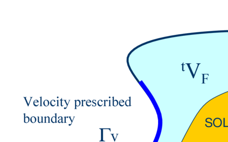
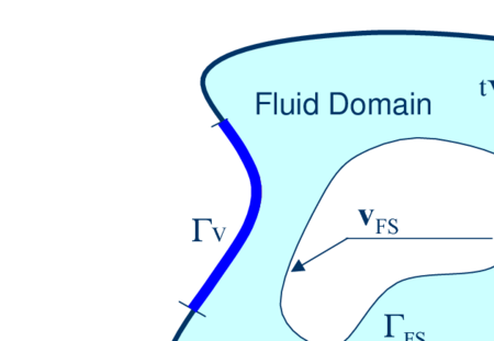
Figure 5 shows a typical domain with external boundaries and where the velocity and the surface tractions are prescribed, respectively. The domain is formed by fluid () and solid () subdomains (i.e. ). Both subdomains interact at a common boundary where the surface tractions and the kinematic variables (displacements, velocities and acelerations) are the same for both subdomains. Note that both set of variables (the surface tractions and the kinematic variables) are equivalent in the equilibrium configuration.
|
|
| Figure 5: Split of the analysis domain into fluid and solid subdomains. Equality of surface tractions and kinematic variables at the common interface | |
Let us define and the set of variables defining the kinematics and the stress-strain fields at the solid and fluid domains at time , respectively, i.e.
|
where is the nodal coordinate vector, u, v and a are the vector of displacements, velocities and accelerations, respectively, and are the strain vector, the strain-rate (or rate of deformation) vectors and the Cauchy stress vector, respectively, is the temperature and subscripts and denote the variables in the fluid and solid domains, respectively. In the discretized problem, a bar over these variables denotes nodal values.
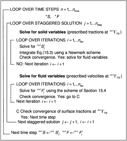
The coupled fluid-structure interaction (FSI) problem of Figure 4 is solved, in this work, using the following strongly coupled staggered scheme:
- We assume that the variables in the solid and fluid domains at time ( and ) are known.
- Solve for the variables at the solid domain at time () under prescribed surface tractions at the fluid-solid boundary . The boundary conditions at the part of the external boundary intersecting the domain are the standard ones in solid mechanics.
The variables at the solid domain are found via the integration of the equations of dynamic motion in the solid written as [40]
|
|
(14) |
where is the vector of nodal accelerations and and are the mass matrix, the internal node force vector and the external nodal force vector in the solid domain. The time integration of Eq.(14) is performed using a standard Newmark method.
Solve for the variables at the fluid domain at time () under prescribed surface tractions at the external boundary and prescribed velocities at the external and internal boundaries and , respectively. An incremental iterative scheme is implemented within each time step to account for non linear geometrical and material effects.
Iterate between 1 and 2 until convergence.
The above FSI solution algorithm is shown schematically in Box II.
|
5 Generation of a new mesh
One of the key points for the success of the PFEM is the fast regeneration of a mesh at every time step on the basis of the position of the nodes in the space domain. Indeed, any fast meshing algorithm can be used for this purpose. In our work the mesh is generated at each time step using the so called extended Delaunay tesselation (EDT) presented in [11,13,14]. The EDT allows one to generate non standard meshes combining elements of arbitrary polyhedrical shapes (triangles, quadrilaterals and other polygons in 2D and tetrahedra, hexahedra and arbitrary polyhedra in 3D) in a computing time of order , where is the total number of nodes in the mesh (Figure 6). The continuous shape functions of the elements can be simply obtained using the so called meshless finite element interpolation (MFEM). In our work the simpler linear C interpolation has been chosen [11,13,14].
|
| Figure 6: Generation of non standard meshes combining different polygons (in 2D) and polyhedra (in 3D) using the extended Delaunay technique. |
Figure 7 shows the evolution of the CPU time required for generating the mesh, for solving the system of equations and for assembling such a system in terms of the number of nodes. the numbers correspond to the solution of a 3D flow in an open channel with the PFEM [32]. The figure shows the CPU time in seconds for each time step of the algorithm of Section 3.2. We see that the CPU time required for meshing grows linearly with the number of nodes, as expected. Note also that the CPU time for solving the equations exceeds that required for meshing as the number of nodes increases. This situation has been found in all the problems solved with the PFEM. As a general rule for large 3D problems meshing consumes around 30% of the total CPU time for each time step, while the solution of the equations and the assembling of the system consume approximately 40% and 20% of the CPU time for each time step, respectively. These figures prove that the generation of the mesh has an acceptable cost in the PFEM.
|
| Figure 7: 3D flow problem solved with the PFEM. CPU time for meshing, assembling and solving the system of equations at each time step in terms of the number of nodes |
6 Identification of boundary surfaces
One of the main tasks in the PFEM is the correct definition of the boundary domain. Boundary nodes are sometimes explicitly identified. In other cases, the total set of nodes is the only information available and the algorithm must recognize the boundary nodes.
In our work we use an extended Delaunay partition for recognizing boundary nodes. Considering that the nodes follow a variable distribution, where is typically the minimum distance between two nodes, the following criterion has been used. All nodes on an empty sphere with a radius greater than , are considered as boundary nodes. In practice is a parameter close to, but greater than one. Values of ranging between 1.3 and 1.5 have been found to be optimal in all examples analyzed. This criterion is coincident with the Alpha Shape concept [8]. Figure 8 shows an example of the boundary recognition using the Alpha Shape technique.
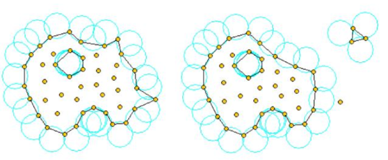
|
| Figure 8: Identification of individual particles (or a group of particles) starting from a given collection of nodes. |
Once a decision has been made concerning which nodes are on the boundaries, the boundary surface is defined by all the polyhedral surfaces (or polygons in 2D) having all their nodes on the boundary and belonging to just one polyhedron.
The method described also allows one to identify isolated fluid particles outside the main fluid domain. These particles are treated as part of the external boundary where the pressure is fixed to the atmospheric value. We recall that each particle is a material point characterized by the density of the solid or fluid domain to which it belongs. The mass which is lost when a boundary element is eliminated due to departure of a node (a particle) from the main analysis domain is again regained when the “flying” node falls down and a new boundary element is created by the Alpha Shape algorithm (Figures 2 and 8).
The boundary recognition method above described is also useful for detecting contact conditions between the fluid domain and a fixed boundary, as well as between different solids interacting with each other. The contact detection procedure is detailed in the next section.
We note that the main difference between the PFEM and the classical FEM is just the remeshing technique and the identification of the domain boundary at each time step. The rest of the steps in the computation are coincident with those of the classical FEM.
7 Treatment of contact conditions in the PFEM
7.1 Contact between the fluid and a fixed boundary
The motion of the solid is governed by the action of the fluid flow forces induced by the pressure and the viscous stresses acting at the common boundary , as mentioned above.
The condition of prescribed velocities at the fixed boundaries in the PFEM are applied in strong form to the boundary nodes. These nodes might belong to fixed external boundaries or to moving boundaries linked to the interacting solids. Contact between the fluid particles and the fixed boundaries is accounted for by the incompressibility condition which naturally prevents the fluid nodes to penetrate into the solid boundaries (Figure 9). This simple way to treat the fluid-wall contact at mesh generation level is a distinct and attractive feature of the PFEM formulation.
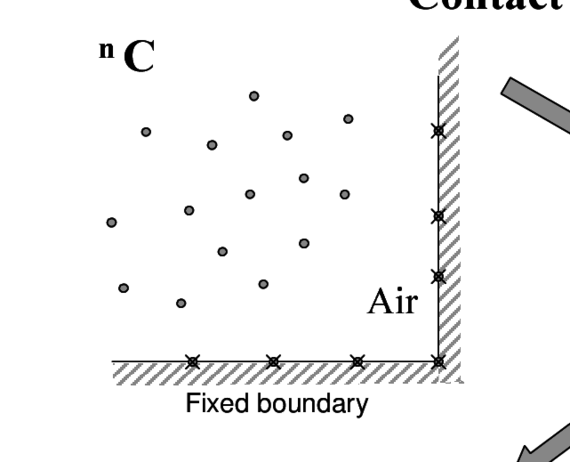
|
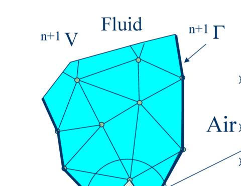
|
| Figure 9: Automatic treatment of contact conditions at the fluid-wall interface | |
7.2 Contact between solid-solid interfaces
The contact between two solid interfaces is simply treated by introducing a layer of contact elements between the two interacting solid interfaces. This layer is automatically created during the mesh generation step by prescribing a minimum distance () between two solid boundaries. If the distance exceeds the minimum value () then the generated elements are treated as fluid elements. Otherwise the elements are treated as contact elements where a relationship between the tangential and normal forces and the corresponding displacement is introduced so as to model elastic and frictional contact effects in the normal and tangential directions, respectively (Figure 10).
This algorithm has proven to be very effective and it allows to identifying and modeling complex frictional contact conditions between two or more interacting bodies moving in water in an extremely simple manner. Of course the accuracy of this contact model depends on the critical distance above mentioned.
This contact algorithm can also be used effectively to model frictional contact conditions between rigid or elastic solids in standard structural mechanics applications. Figures 11–14 show examples of application of the contact algorithm to the bumping of a ball falling in a container, the failure of an arch formed by a collection of stone blocks under a seismic loading and the motion of five tetrapods as they fall and slip over an inclined plane, respectively. The images in Figures 11 and 14 show explicitely the layer of contact elements which controls the accuracy of the contact algorithm.
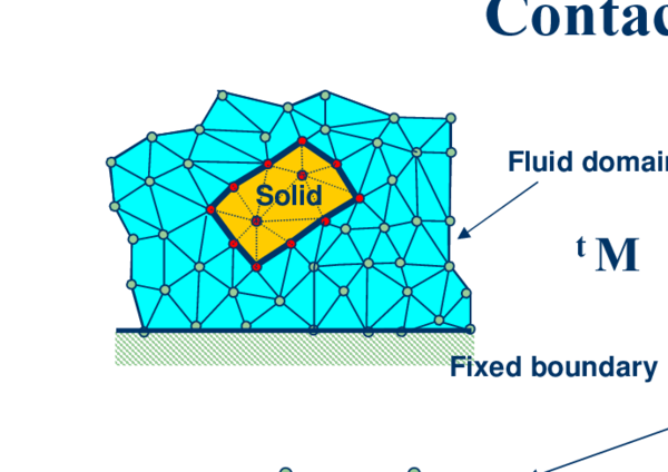
|
| Figure 10: Contact conditions at a solid-solid interface |
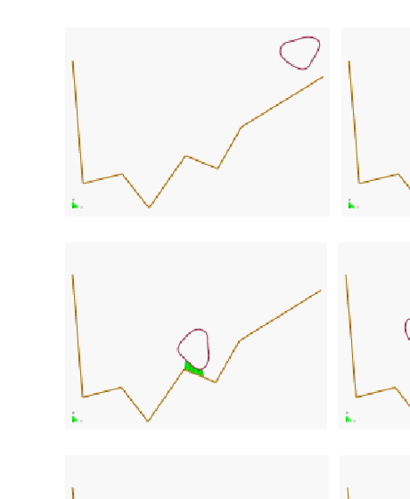
|
| Figure 11: Bumping of a ball within a container. The layer of contact elements is shown at each contact instant |
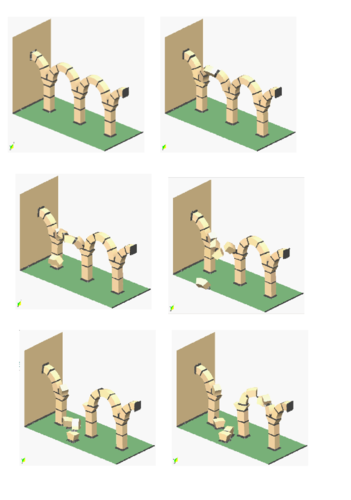
|
| Figure 12: Failure of an arch formed by stone blocks under seismic loading |
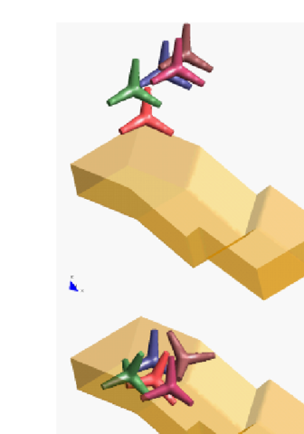
|
| Figure 13: Motion of five tetrapods on an inclined plane |
8 Modeling of bed erosion
Prediction of bed erosion and sediment transport in open channel flows are important tasks in many areas of river and environmental engineering. Bed erosion can lead to instabilities of the river basin slopes. It can also undermine the foundation of bridge piles thereby favouring structural failure. Modeling of bed erosion is also relevant for predicting the evolution of surface material dragged in earth dams in overspill situations. Bed erosion is one of the main causes of environmental damage in floods.
Bed erosion models are traditionally based on a relationship between the rate of erosion and the shear stress level [16,36]. The effect of water velocity on soil erosion was studied in [34]. In a recent work we have proposed an extension of the PFEM to model bed erosion [31]. The erosion model is based on the frictional work at the bed surface originated by the shear stresses in the fluid. The resulting erosion model resembles Archard law typically used for modeling abrasive wear in surfaces under frictional contact conditions [1,24].
The algorithm for modeling the erosion of soil/rock particles at the fluid bed is the following:
- Compute at every point of the bed surface the resultant tangential stress induced by the fluid motion. In 3D problems where and are the tangential stresses in the plane defined by the normal direction at the bed node. The value of for 2D problems can be estimated as follows:
(15.a) with
(15.b) where is the modulus of the tangential velocity at the node and is a prescribed distance along the normal of the bed node . Typically is of the order of magnitude of the smallest fluid element adjacent to node (Figure 15).
- Compute the frictional work originated by the tangential stresses at the bed surface as
(16) Eq.(16) is integrated in time using a simple scheme as
(17) - The onset of erosion at a bed point occurs when exceeds a critical threshold value defined empirically according to the specific properties of the bed material.
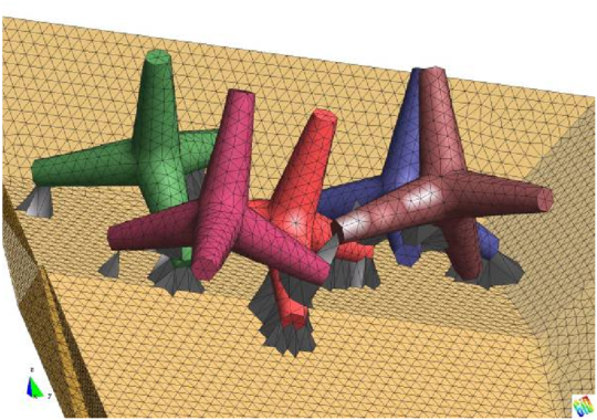
|
| Figure 14: Detail of five tetrapods on an inclined plane. The layer of elements modeling the frictional contact conditions is shown |
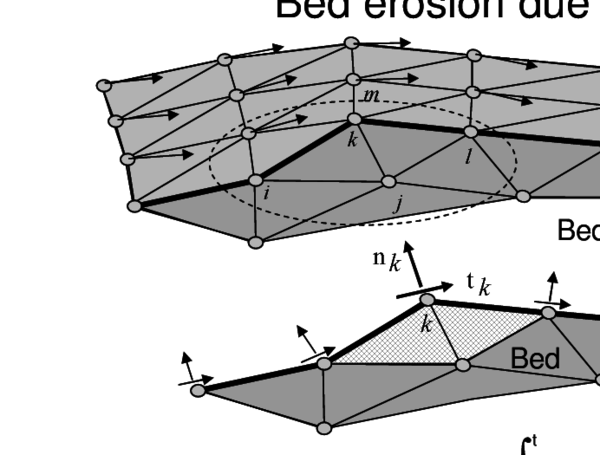
|
| Figure 15: Modeling of bed erosion by dragging of bed material |
- If at a bed node, then the node is detached from the bed region and it is allowed to move with the fluid flow, i.e. it becomes a fluid node. As a consequence, the mass of the patch of bed elements surrounding the bed node vanishes in the bed domain and it is transferred to the new fluid node. This mass is subsequently transported with the fluid. Conservation of mass of the bed particles within the fluid is guaranteed by changing the density of the new fluid node so that the mass of the suspended sediment traveling with the fluid equals the mass originally assigned to the bed node. Recall that the mass assigned to a node is computed by multiplying the node density by the tributary domain of the node.
- Sediment deposition can be modeled by an inverse process to that described in the previous step. Hence, a suspended node adjacent to the bed surface with a velocity below a threshold value is assigned to the bed surface. This automatically leads to the generation of new bed elements adjacent to the boundary of the bed region. The original mass of the bed region is recovered by adjusting the density of the newly generated bed elements.
Figure 15 shows an schematic view of the bed erosion algorithm proposed.
9 Examples
The examples presented below show the applicability of the PFEM to solve problems involving large motions of the free surface, fluid-multibody interactions, bed erosion and melting and dripping of polymers in fire situations.
9.1 Rigid objects falling into water
The analysis of the motion of submerged or floating objects in water is of great interest in many areas of harbour and coastal engineering and naval architecture among others.
Figure 16 shows the penetration and evolution of a cube and a cylinder of rigid shape in a container with water. The colours denote the different sizes of the elements at several times. In order to increase the accuracy of the FSI problem smaller size elements have been generated in the vicinity of the moving bodies during their motion (Figure 17).
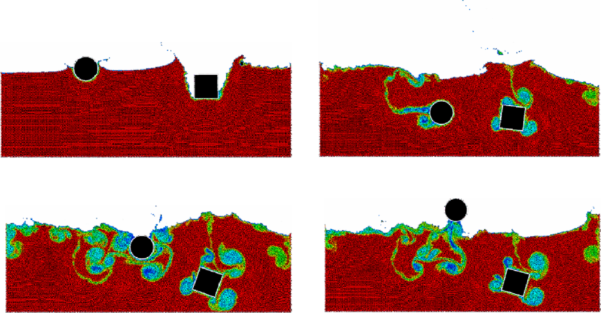
|
| Figure 16: 2D simulation of the penetration and evolution of a cube and a cylinder in a water container. The colours denote the different sizes of the elements at several times |
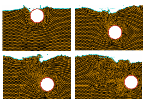
|
| Figure 17: Detail of element sizes during the motion of a rigid cylinder within a water container |
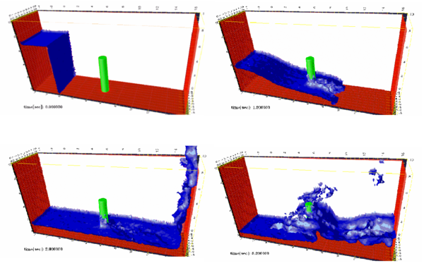
|

|
| Figure 18: Evolution of a water column within a prismatic container including a vertical cylinder | |
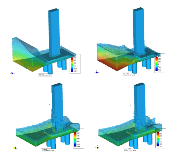
|
| Figure 19: Impact of a wave on a prismatic column on a slab sustained by four pillars. |
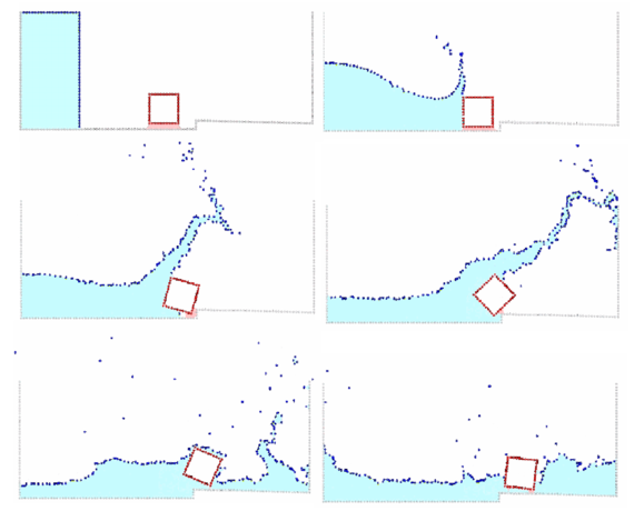
|
| Figure 20: Dragging of a cubic object by a water stream. |
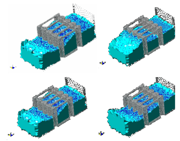
|
| Figure 21: Interaction of a wave with a vertical pier formed by reinforced concrete cylinders. |
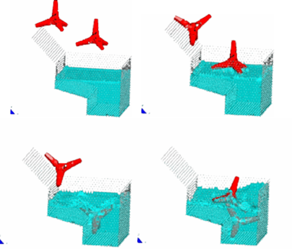
|
| Figure 22: Motion of two tetrapods falling in a water container. |
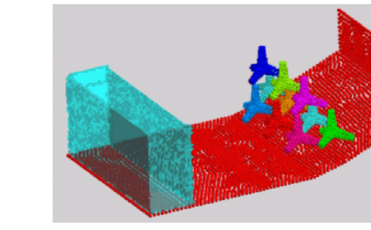
|

|
| Figure 23: Motion of ten tetrapods on a slope under an incident wave. | |
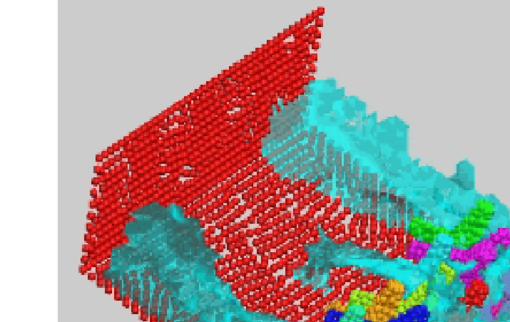
|
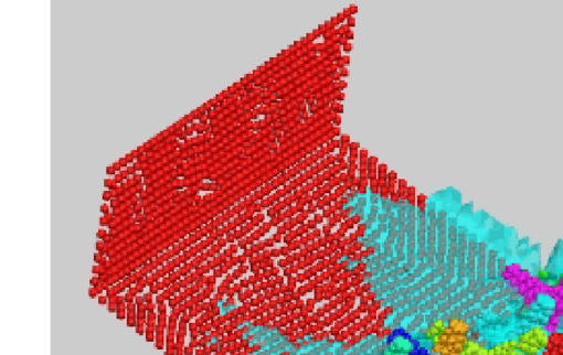
|
| Figure 24: Detail of the motion of ten tetrapods on a slope under an incident wave. The figure shows the complex interactions between the water particles and the tetrapods. | |
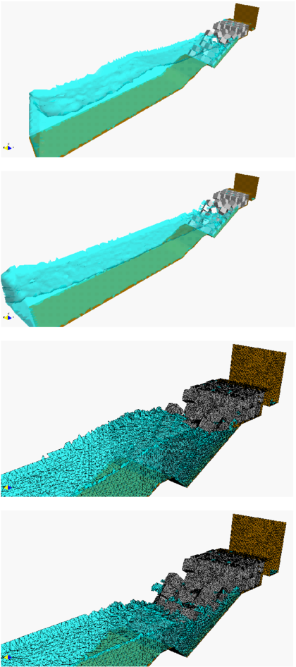
|
| Figure 25: Effect of breaking waves on a breakwater slope containing reinforced concrete blocks. Detail of the mesh of 4-noded tetrahedra near the slope at two different times |
9.2 Impact of water streams on rigid structures
Figure 18 shows an example of a wave breaking within a prismatic container including a vertical cylinder. Figure 19 shows the impact of a wave on a vertical column sustained by four pillars. The objective of this example was to model the impact of a water stream on a bridge pier accounting for the foundation effects.
9.3 Dragging of objects by water streams
Figure 20 shows the effect of a wave impacting on a rigid cube representing a vehicle. This situation is typical in flooding and Tsunami situations. Note the layer of contact elements modeling the frictional contact conditions between the cube and the bottom surface.
9.4 Impact of sea waves on piers and breakwaters
Figure 21 shows the 3D simulation of the interaction of a wave with a vertical pier formed by a collection of reinforced concrete cylinders.
Figure 22 shows the simulation of the falling of two tetrapods in a water container. Figure 23 shows the motion of a collection of ten tetrapods placed in the slope of a breakwaters under an incident wave.
Figure 24 shows a detail of the complex three-dimensional interactions between water particles and tetrapods and between the tetrapods themselves.
Figures 25 and 26 show the analysis of the effect of breaking waves on two different sites of a breakwater containing reinforced concrete blocks (each one of mts). The figures correspond to the study of Langosteira harbour in La Coruna, Spain using PFEM.
Figure 27 displays the effect of an overtopping wave on a truck circulating by the perimetral road of the harbour adjacent to the breakwater.
9.5 Erosion of a 3D earth dam due to an overspill stream
We present a simple, schematic, but very illustrative example showing the potential of the PFEM to model bed erosion in free surface flows.
The example represents the erosion of an earth dam under a water stream running over the dam top. A schematic geometry of the dam has been chosen to simplify the computations. Sediment deposition is not considered in the solution. The images of Figure 28 show the progressive erosion of the dam until the whole dam is dragged out by the fluid flow.
Other applications of the PFEM to bed erosion problems can be found in [31].
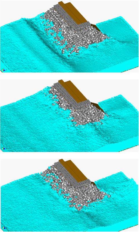
|
| Figure 26: Study of breaking waves on the edge of a breakwater structure formed by reinforced concrete blocks |
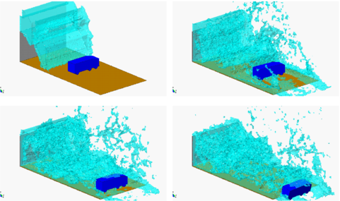
|
| Figure 27: Effect of an overtopping wave on a truck passing by the perimetral road of a harbour adjacent to the breakwater |
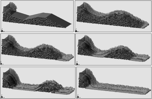
|
| Figure 28: Erosion of a 3D earth dam due to an overspill stream. |
9.6 Melting and spread of polymer objects in fire
In the next example shown the PFEM is used to simulate an experiment performed at the National Institute for Stanford and Technology (NIST) in which a slab of polymeric material is mounted vertically and exposed to uniform radiant heating on one face. It is assumed that the polymer melt flow is governed by the equations of an incompressible fluid with a temperature dependent viscosity. A quasi-rigid behaviour of the polymer object at room temperature is reproduced by using a very high value of the viscosity parameter. As temperature increases in the thermoplastic object due to heat exposure, the viscosity decreases in several orders of magnitude as a function of temperature and this induces the melt and flow of the particles in the heated zone. Polymer melt is captured by a pan below the sample.
A schematic of the apparatus used in the experiments is shown in Figure 29. A rectangular polymeric sample of dimensions 10 cm high by 10 cm wide by 2.5 cm thick is mounted upright and exposed to uniform heating on one face from a radiant cone heater placed on its side. The sample is insulated on its lateral and rear faces. The melt flows down the heated face of the sample and drips onto a surface below. A load cell monitors the mass of polymer remaining in the sample, and a laboratory balance measures the mass of polymer falling onto the catch surface. Details of the experimental setup are given in [4].
Figure 29 shows all three curves of viscosity vs. temperature for the polypropylene type PP702N, a low viscosity commercial injection molding resin formulation. The relationship used in the model, as shown by the black line, connects the curve for the undegraded polymer to points A and B extrapolated from the viscosity curve for each melt sample to the temperature at which the sample was formed. The result is an empirical viscosity-temperature curve that implicitly accounts for molecular weight changes.
The finite element mesh used for the analysis has 3098 nodes and 5832 triangular elements. No nodes are added during the course of the run. The addition of a catch pan to capture the dripping polymer melt tests the ability of the PFEM model to recover mass when a particle or set of particles reaches the catch surface. For this problem, heat flux is only applied to free surfaces above the midpoint between the catch pan and the base of the sample. However, every free surface is subject to radiative and convective heat losses. To keep the melt fluid, the catch pan is set to a temperature of 600 K. Figure 30 shows four snapshots of the time evolution of the melt flow into the catch pan.
To test the ability of the PFEM to solve this type of problem in three dimensions, a 3D problem for flow from a heated sample was run. The same boundary conditions are used as in the 2D problem illustrated in Figure 29, but the initial dimensions of the sample are reduced to cm. The initial size of the model is 22475 nodes and 97600 four-noded tetrahedra. The shape of the surface and temperature field at different times after heating begins are shown in Figure 32.
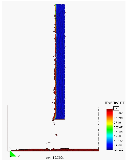
|
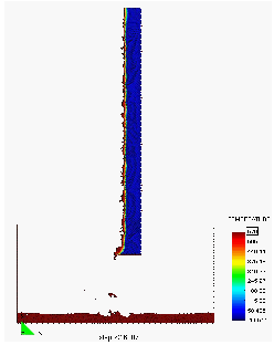
|
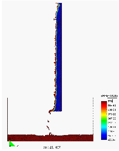
|
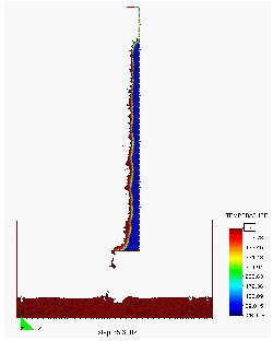
|
| Figure 30: Evolution of the melt flow into the catch pan at t = 400s, 550s, 700s and 1000s | |
Although the resolution for this problem is not fine enough to achieve high accuracy, the qualitative agreement of the 3D model with 2D flow and the ability to carry out this problem in a reasonable amount of time suggest that the PFEM can be used to model melt flow and spread of complex 3D polymer geometry.
Figure 31 shows results for the analysis of the melt flow of a triangular thermoplastic object into a catch pan. The material properties for the polymer are the same as for the previous example. The PFEM succeeds to predicting in a very realistic manner the progressive melting and slip of the polymer particles along the vertical wall separating the triangular object and the catch pan. The analysis follows until the whole object has fully melt and its mass is transferred to the catch pan.
We note that the total mass was preserved with an accuracy of 0.5% in both these studies. Gasification, in-depth absorption or radiation were not taken into account in these analysis. More examples of application of PFEM to the melting and dripping of polymers are reported in [33].
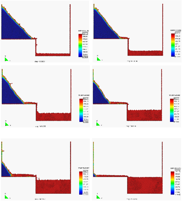
|
| Figure 31: Melt flow of a heated triangular object into a catch pan. |
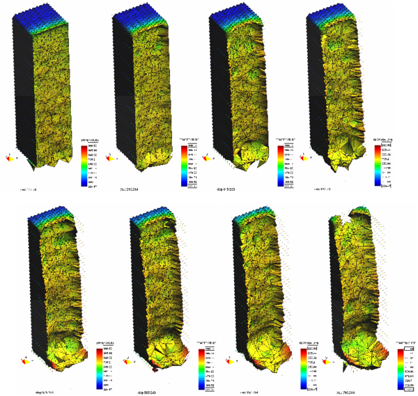
|
| Figure 32: Solution of a 3D polymer melt problem with the PFEM. Melt flow from a heated prismatic sample at different times. |
10 Conclusions
The particle finite element method (PFEM) is ideal to treat problems involving fluid-structure interaction, large motion of fluid or solid particles, surface waves, water splashing, separation of water drops, frictional contact situations between fluid-solid and solid-solid interfaces, bed erosion, coupled thermal effects, melting and dripping of objects, etc. The success of the PFEM lies in the accurate and efficient solution of the equations of an incompressible fluid and of solid dynamics using an updated Lagrangian formulation and a stabilized finite element method, allowing the use of low order elements with equal order interpolation for all the variables. Other essential solution ingredients are the efficient regeneration of the finite element mesh using an extended Delaunay tesselation, the identification of the boundary nodes using the Alpha-Shape technique and the simple algorithm to treat frictional contact conditions at fluid-solid and solid-solid interfaces via mesh generation. The examples presented have shown the great potential of the PFEM for solving a wide class of practical FSI problems in engineering. Examples of validation of the PFEM results with data from experimental tests are reported in [17].
Acknowledgements
Thanks are given to Mrs. M. de Mier for many useful suggestions. This research was partially supported by project SEDUREC of the Consolider Programme of the Ministerio de Educación y Ciencia (MEC) of Spain, project XPRES of the National I+D Programme of MEC (Spain) and project SAYOM of CDTI Spain. Thanks are also given to the Spanish construction company Dragados for financial support for the study of harbour engineering problems.
BIBLIOGRAPHY
[1] J.F. Archard, Contact and rubbing of flat surfaces, J. Appl. Phys. 24(8) (1953) 981–988.
[2] R. Aubry, S.R. Idelsohn, E. Oñate, Particle finite element method in fluid mechanics including thermal convection-diffusion, Computer & Structures 83(17-18) (2005) 1459–1475.
[3] K.M. Butler, T.J. Ohlemiller, G.T. Linteris, A Progress Report on Numerical Modeling of Experimental Polymer Melt Flow Behavior, Interflam (2004) 937–948.
[4] K.M. Butler, E. Oñate, S.R. Idelsohn, R. Rossi, Modeling and simulation of the melting of polymers under fire conditions using the particle finite element method, 11th Int. Fire Science & Engineering Conference, University of London, Royal Halbway College, UK, (2007) 3-5 September.
[5] R. Codina, O.C. Zienkiewicz, CBS versus GLS stabilization of the incompressible Navier-Stokes equations and the role of the time step as stabilization parameter, Communications in Numerical Methods in Engineering (2002) 18(2) (2002) 99–112.
[6] F. Del Pin, S.R. Idelsohn, E. Oñate, R. Aubry, The ALE/Lagrangian particle finite element method: A new approach to computation of free-surface flows and fluid-object interactions. Computers & Fluids 36 (2007) 27–38.
[7] J. Donea, A. Huerta, Finite element method for flow problems, J. Wiley, (2003).
[8] H. Edelsbrunner, E.P. Mucke, Three dimensional alpha shapes, ACM Trans. Graphics 13 (1999) 43–72.
[9] J. García, E. Oñate, An unstructured finite element solver for ship hydrodynamic problems, J. Appl. Mech. 70 (2003) 18–26.
[10] S.R. Idelsohn, E. Oñate, F. Del Pin, N. Calvo, Lagrangian formulation: the only way to solve some free-surface fluid mechanics problems, Fith World Congress on Computational Mechanics, H.A. Mang, F.G. Rammerstorfer, J. Eberhardsteiner (eds), July 7–12, Viena, Austria, (2002).
[11] S.R. Idelsohn, E. Oñate, N. Calvo, F. Del Pin, The meshless finite element method, Int. J. Num. Meth. Engng. 58(6) (2003a) 893–912.
[12] S.R. Idelsohn, E. Oñate, F. Del Pin, A lagrangian meshless finite element method applied to fluid-structure interaction problems, Computer and Structures 81 (2003b) 655–671.
[13] S.R. Idelsohn, N. Calvo, E. Oñate, Polyhedrization of an arbitrary point set, Comput. Method Appl. Mech. Engng. 192(22-24) (2003c) 2649–2668.
[14] S.R. Idelsohn, E. Oñate, F. Del Pin, The particle finite element method: a powerful tool to solve incompressible flows with free-surfaces and breaking waves, Int. J. Num. Meth. Engng. 61 (2004) 964-989.
[15] S.R. Idelsohn, E. Oñate, F. Del Pin, N. Calvo, Fluid-structure interaction using the particle finite element method, Comput. Meth. Appl. Mech. Engng. 195 (2006) 2100-2113.
[16] A. Kovacs, G. Parker, A new vectorial bedload formulation and its application to the time evolution of straight river channels, J. Fluid Mech. 267 (1994) 153–183.
[17] A. Larese, R. Rossi, E. Oñate, S.R. Idelsohn, Validation of the Particle Finite Element Method (PFEM) for simulation of free surface flows, submitted to Engineering Computations 25 (4) (2008) 385–425.
[18] R. Ohayon, Fluid-structure interaction problem, in: E. Stein, R. de Borst, T.J.R. Hugues (Eds.), Enciclopedia of Computatinal Mechanics, Vol. 2, (J. Wiley, 2004) 683–694.
[19] E. Oñate, Derivation of stabilized equations for advective-diffusive transport and fluid flow problems, Comput. Meth. Appl. Mech. Engng. 151 (1998) 233–267.
[20] E. Oñate, A stabilized finite element method for incompressible viscous flows using a finite increment calculus formulation, Comp. Meth. Appl. Mech. Engng. 182(1–2) (2000) 355–370.
[21] E. Oñate, Possibilities of finite calculus in computational mechanics Int. J. Num. Meth. Engng. 60(1) (2004) 255–281.
[22] E. Oñate, S.R. Idelsohn, A mesh free finite point method for advective-diffusive transport and fluid flow problems, Computational Mechanics 21 (1998) 283–292.
[23] E. Oñate, J. García, A finite element method for fluid-structure interaction with surface waves using a finite calculus formulation, Comput. Meth. Appl. Mech. Engrg. 191 (2001) 635–660.
[24] E. Oñate, J. Rojek, Combination of discrete element and finite element method for dynamic analysis of geomechanic problems, Comput. Meth. Appl. Mech. Engrg. 193 (2004) 3087–3128.
[25] E. Oñate, C. Sacco, S.R. Idelsohn, A finite point method for incompressible flow problems, Comput. Visual. in Science 2 (2000) 67–75.
[26] E. Oñate, S.R. Idelsohn, F. Del Pin, Lagrangian formulation for incompressible fluids using finite calculus and the finite element method, Numerical Methods for Scientific Computing Variational Problems and Applications, Y Kuznetsov, P Neittanmaki, O Pironneau (Eds.), CIMNE, Barcelona (2003).
[27] E. Oñate, J. García, S.R. Idelsohn, Ship hydrodynamics, in: E. Stein, R. de Borst, T.J.R. Hughes (Eds), Encyclopedia of Computational Mechanics, J. Wiley, Vol 3, (2004a) 579–610.
[28] E. Oñate, S.R. Idelsohn, F. Del Pin, R. Aubry, The particle finite element method. An overview, Int. J. Comput. Methods 1(2) (2004b) 267-307.
[29] E. Oñate, A. Valls, J. García, FIC/FEM formulation with matrix stabilizing terms for incompressible flows at low and high Reynold's numbers, Computational Mechanics 38 (4-5) (2006a) 440-455.
[30] E. Oñate, J. García, S.R. Idelsohn, F. Del Pin, FIC formulations for finite element analysis of incompressible flows. Eulerian, ALE and Lagrangian approaches, Comput. Meth. Appl. Mech. Engng. 195 (23-24) (2006b) 3001-3037.
[31] E. Oñate, M.A. Celigueta, S.R. Idelsohn, Modeling bed erosion in free surface flows by the Particle Finite Element Method, Acta Geotechnia 1 (4) (2006c) 237-252.
[32] E. Oñate, S.R. Idelsohn, M.A. Celigueta, R. Rossi, Advances in the particle finite element method for the analysis of fluid-multibody interaction and bed erosion in free surface flows, Comput. Meth. Appl. Mech. Engng. 197 (19-20) (2008) 1777-1800.
[33] E. Oñate, R. Rossi, S.R. Idelsohn, K. Butler, Melting and spread of polymers in fire with the particle finite element method. Submitted to Int. J. Num. Meth. in Engng., (2009).
[34] D.B. Parker, T.G. Michel, J.L. Smith, Compaction and water velocity effects on soil erosion in shallow flow, J. Irrigation and Drainage Engineering 121 (1995) 170–178.
[35] T.E. Tezduyar, Finite element method for fluid dynamics with moving boundaries and interface, in: E. Stein, R. de Borst, T.J.R. Hugues (Eds.), Enciclopedia of Computatinal Mechanics, Vol. 3, (J. Wiley, 2004) 545–578.
[36] C.F. Wan, R. Fell, Investigation of erosion of soils in embankment dams, J. Geotechnical and Geoenvironmental Engineering 130 (2004) 373–380.
[37] O.C. Zienkiewicz, R.L. Taylor, P. Nithiarasu, The finite element method for fluid dynamics, Elsevier, (2006).
[38] O.C. Zienkiewicz, P.C. Jain, E. Oñate, Flow of solids during forming and extrusion: Some aspects of numerical solutions. Int. Journal of Solids and Structures (1978) 14 15–38.
[39] O.C. Zienkiewicz, E. Oñate, J.C. Heinrich, A general formulation for the coupled thermal flow of metals using finite elements. Int. Journal for Numerical Methods in Engineering (1981) 17 1497–1514.
[40] O.C. Zienkiewicz, R.L. Taylor, The finite element method for solid and structural mechanics, Elsevier, (2005).
APPENDIX
The matrices and vectors in Eqs.(8)-(11) for a 4-noded tetrahedron are:
|
|
|
|
|
|
|
|
|
|
|
|
|
|
|
|
|
|
|
|
In above equations indexes run from 1 to the number of element nodes (4 for a tetrahedron), is the heat flow prescribed at the external boundary , t is the surface traction vector and and are the element volume and the element boundary, respectively.
Document information
Published on 01/01/2010
Licence: CC BY-NC-SA license
Share this document
claim authorship
Are you one of the authors of this document?

