Evaluating manoeuvering and seakeeping performance of a surface effect ship

Latest revision as of 12:20, 14 March 2018

Project funded under Navy Grant N62909-10-1-7053 issued by Office of Naval Research Global

1. Hydrodynamic solver: Mathematical modelling

1.1 Governing equations

We consider the first order diffraction-radiation problem of a ship moving on the horizontal plane. The two dimensional movement of the ship is identified by ${\boldsymbol {v}}_{b}({\boldsymbol {x}})={\boldsymbol {T}}_{b}+$ ${\boldsymbol {W}}_{b}\times ({\boldsymbol {x}}-{\boldsymbol {x}}_{G})$ , where ${\boldsymbol {T}}_{b}$ and ${\boldsymbol {W}}_{b}$ are the linear and angular velocity of the ship. We assume that the flow is incompressible and irrotational, so that the velocity field ${\textstyle {\boldsymbol {v}}}$ , is derived from a potential function ${\textstyle \varphi }$ as: ${\textstyle {\boldsymbol {v}}=\nabla \varphi }$ . The following assumptions are made on the order of magnitude of the velocity components and free surface elevation $\zeta$ :

{\begin{array}{c}V_{b}\sim O(1);{\mbox{ }}{\varphi }_{x}\sim O(1);{\mbox{ }}{\varphi }_{y}\sim O(1);\\{\varphi }_{z}\sim O(\epsilon );{\mbox{ }}{\varphi }_{\alpha \beta }\sim O(\epsilon );{\mbox{ }}{\zeta }_{x}\sim O(1);{\mbox{ }}{\mbox{ }}{\zeta }_{y}\sim O(1);\end{array}}

(1)

Based on the previous assumption, the governing equations for the first order diffraction-radiation wave problem are:

{\begin{array}{c}{\nabla }^{2}\varphi =0\\{\partial }_{t}\varphi +{\boldsymbol {u}}\cdot {\nabla }_{h}\varphi +{\frac {1}{2}}{\nabla }_{h}\varphi \cdot {\nabla }_{h}\varphi +P/\rho +g\zeta =0\\{\partial }_{t}\zeta +({\boldsymbol {u}}+{\nabla }_{h}\varphi )\cdot {\nabla }_{h}\zeta -{\varphi }_{z}=0\\\left({\boldsymbol {u}}+\nabla \varphi \right)\cdot {\boldsymbol {n}}_{b}={\boldsymbol {v}}_{b}\cdot {\boldsymbol {n}}_{b}\\{\varphi }_{z}=0\end{array}}

(2)

where ${\nabla }_{h}=({\partial }_{x},{\partial }_{y})$ is the gradient in the horizontal plane, $\Omega$ is the fluid domain, ${\Gamma }_{b}$ represents the wetted surface of the ship, $H$ is the water depth, ${\boldsymbol {v}}_{b}$ is the local ship velocity of a point over the wetted surface, ${\boldsymbol {n}}_{b}$ is the normal of the ship wetted surface pointing outwards the ship, ${\boldsymbol {u}}$ is the water current, and $P$ is the free surface pressure. Once the velocity potential is obtained, the pressure field is obtained straightforward using the Bernoulli equation:

(3)

1.2 Velocity potential decomposition

In order to solve the governing equations provided in Eq.(2), a velocity potential decomposition is introduced. Let ${\textstyle \varphi }$ and ${\textstyle \zeta }$ be such that;

(4)

Then, we can split the governing equations into the following sets of equations:

Set 1:

(5)

Set 2:

{\begin{array}{c}{\nabla }^{2}\phi =0\\{\partial }_{t}\phi +{\boldsymbol {u}}\cdot {\nabla }_{h}\phi +{\frac {1}{2}}{\nabla }_{h}\phi \cdot {\nabla }_{h}\phi +{\nabla }_{h}\psi \cdot {\nabla }_{h}\phi +{\frac {1}{2}}{\nabla }_{h}\psi \cdot {\nabla }_{h}\psi +P/\rho +g\eta =0\\{\partial }_{t}\eta +({\boldsymbol {u}}+{\nabla }_{h}\phi +{\nabla }_{h}\psi )\cdot {\nabla }_{h}\eta +({\nabla }_{h}\phi +{\nabla }_{h}\psi )\cdot {\nabla }_{h}\xi -{\phi }_{z}=0\\\nabla \phi \cdot {\boldsymbol {n}}_{b}=\left({\boldsymbol {v}}_{b}-\nabla \psi -{\boldsymbol {u}}\right)\cdot {\boldsymbol {n}}_{b}\\{\phi }_{z}=0\end{array}}

(6)

The first set of equation, Eq.(5), has an analytical solution (known as Airy waves):

{\begin{array}{c}\psi ={\sum }_{i}{\frac {cosh\left(\vert {\boldsymbol {k}}_{i}\vert (H+z)\right)}{cosh\left(\vert {\boldsymbol {k}}_{i}\vert H\right)}}cos\left({\boldsymbol {k}}_{i}\cdot ({\boldsymbol {x}}-{\boldsymbol {u}}t)-{\omega }_{i}t+{\alpha }_{i}\right);\\\xi =\sum _{i}A_{i}sin\left({\boldsymbol {k}}_{i}\cdot ({\boldsymbol {x}}-{\boldsymbol {u}}t)-{\omega }_{i}t+{\alpha }_{i}\right)\end{array}}

(7)

where $A_{i}$ are the wave amplitudes; ${\omega }_{i}$ are the wave frequencies; ${\boldsymbol {k}}_{i}$ are the wave numbers; ${\alpha }_{i}$ are the wave phases. From this point on, we will refer to $\psi$ as the incident potential and $\phi$ as the scattered potential. Also the dispersion relation for Airy waves holds:

(8)

From Airy waves theory, we know that ${\textstyle {\psi }_{\alpha }\sim O(\epsilon )}$ and ${\textstyle {\xi }_{\alpha }\sim O(\epsilon )}$ . Then, the terms ${\nabla }_{h}{\psi }^{2}/2\sim O({\epsilon }^{2})$ , ${\nabla }_{h}\psi \cdot {\nabla }_{h}\xi \sim O({\epsilon }^{2})$ , and ${\nabla }_{h}\psi \cdot {\nabla }_{h}\eta \sim O({\epsilon }^{2})$ . Neglecting these terms in Eq.(6), and using the analytical solutions of Airy waves, the governing equations for the scattered waves potential becomes:

{\begin{array}{c}{\nabla }^{2}\phi =0\\{\partial }_{t}\phi +{\boldsymbol {u}}\cdot {\nabla }_{h}\phi +{\frac {1}{2}}{\nabla }_{h}\phi \cdot {\nabla }_{h}\phi +{\nabla }_{h}\psi \cdot {\nabla }_{h}\phi +P/\rho +g\eta =0\\{\partial }_{t}\eta +({\boldsymbol {u}}+{\nabla }_{h}\phi )\cdot {\nabla }_{h}\eta +{\nabla }_{h}\phi \cdot {\nabla }_{h}\xi -{\phi }_{z}=0\\\nabla \phi \cdot {\boldsymbol {n}}_{b}=\left({\boldsymbol {v}}_{b}-{\boldsymbol {u}}-\nabla \psi \right)\cdot {\boldsymbol {n}}_{b}\\{\phi }_{z}=0\end{array}}

(9)

and

(10)

Notice that the terms ${\nabla }_{h}\psi \cdot {\nabla }_{h}\phi$ and ${\nabla }_{h}\phi \cdot {\nabla }_{h}\xi$ accounts for the deviation of the incident Airy waves due to the fact that the incidents waves are transport by a non-uniform flow field. Also, the terms ${\nabla }_{h}\phi \cdot {\nabla }_{h}\phi$ , $-{\nabla }_{h}{\phi }^{2}/2$ , and ${\nabla }_{h}\phi \cdot {\nabla }_{h}\eta$ are not subject to any kind of linearization, so that there will be no restriction in using non-steady base flows.

1.3 Frame of reference

From a numerical point of view, based on the numerical approaches used in this work, it is convenient to solve Eqs. (9)-(10) in a fix frame of reference rather that on the global frame of reference. Therefore, the aforementioned equations will be solved in a frame of reference fix to the ship. Figure 1 shows the global and local frame of reference. This frame of reference is assumed to match the global frame at time zero. For a observer sitting in the ship, the flow field around the ship will be ${\boldsymbol {U}}({\boldsymbol {x}})={\boldsymbol {u}}-{\boldsymbol {v}}_{b}({\boldsymbol {x}})$ . Therefore, the governing equations in the local frame of reference become:

{\begin{array}{c}{\nabla }^{2}\phi =0\\{\partial }_{t}\phi +{\boldsymbol {U}}\cdot {\nabla }_{h}\phi +{\frac {1}{2}}{\nabla }_{h}\phi \cdot {\nabla }_{h}\phi +{\nabla }_{h}\psi \cdot {\nabla }_{h}\phi +P/\rho +g\eta =0\\{\partial }_{t}\eta +({\boldsymbol {U}}+{\nabla }_{h}\phi )\cdot {\nabla }_{h}\eta +{\nabla }_{h}\phi \cdot {\nabla }_{h}\xi -{\phi }_{z}=0\\\nabla \phi \cdot {\boldsymbol {n}}_{b}=\left(-{\boldsymbol {U}}-\nabla \psi \right)\cdot {\boldsymbol {n}}_{b}\\{\phi }_{z}=0\end{array}}

| style="width: 5px;text-align: right;white-space: nowrap;" | (11) |}

and

(12)

where the incident wave potential and incident wave elevation must be transformed to the local frame of reference.

Figure 1: Global and local frame of reference.

2. Hydrodynamic solver: Numerical modelling

2.1 Laplace equation

The flow is assumed to be incompressible and irrotational. Therefore the Laplace equation has to be fulfilled within the fluid domain. We adopt the finite element method for solving the Laplace equation in the fluid domain.

This formulation has been developed to be used in conjunction with unstructured meshes. The use of unstructured meshes enhances geometry flexibility and speed ups the initial modelling time. An automatic unstructured grid generator based on the advancing front method is used to generate triangular surface grids and tetrahedral volumetric meshes.

Let $Q_{h}^{\ast }$ be the finite element space to interpolate functions, constructed in the usual manner. From this space, we can construct the subspace $Q_{h,\phi }$ , that incorporates the Dirichlet conditions for the potential ${\textstyle \phi }$ . The space of test functions, denoted by $Q_{h}$ , is constructed as $Q_{h,\phi }$ , but with functions vanishing on the Dirichlet boundary. The weak form of the problem can be formulated as:

Find $\left[{\phi }_{h}\phi \right]\in Q_{h,\phi }$ , by solving the discrete variational problem:

(13)

where ${\overset {\frown }{\phi }}_{n}^{B}$ , ${\overset {\frown }{\phi }}_{n}^{R}$ , ${\overset {\frown }{\phi }}_{n}^{Z_{0}}$ and ${\overset {\frown }{\phi }}_{n}^{Z_{-H}}$ are the potential normal gradients corresponding to the Neumann boundary conditions on body, radiation boundary, free surface and bottom, respectively. At this point, it is useful to introduce the associated matrix form

(14)

where ${\overline {\overline {\boldsymbol {L}}}}$ is the standard laplacian matrix, and ${\boldsymbol {b}}^{B}$ , ${\boldsymbol {b}}^{Z_{0}}$ and ${\boldsymbol {b}}^{Z_{-H}}$ are the vector resulting of integrating the corresponding boundary condition term. The bottom boundary is imposed in a natural way when using FEM just doing ${\overset {\frown }{\phi }}_{z}^{Z_{-H}}=0$ . From this point forward we are omitting ${\boldsymbol {b}}^{Z_{-H}}$ .

2.2 Free surface boundary condition

2.2.1 Free surface analysis

Solving the free surface boundary condition efficiently is the key point when dealing with water waves problem. The free surface conditions can be rewritten as:

{\begin{array}{c}{\partial }_{t}\eta +{\underset {Convective{\mbox{ }}term}{\underbrace {{\boldsymbol {U}}\cdot {\nabla }_{h}\eta } }}+{\nabla }_{h}\phi \cdot {\nabla }_{h}\xi -{\phi }_{z}=0\\{\partial }_{t}\phi +{\underset {Convective{\mbox{ }}term}{\underbrace {{\boldsymbol {U}}\cdot {\nabla }_{h}\phi } }}-{\frac {1}{2}}{\nabla }_{h}\phi \cdot {\nabla }_{h}\phi +{\nabla }_{h}\psi \cdot {\nabla }_{h}\phi +P/\rho +g\eta =0\end{array}}

(15)

where ${\boldsymbol {U}}=({\boldsymbol {V}}_{b}+{\nabla }_{h}\phi )$ is the base flow. Linearization respect to this based flow is quite common. Linearizations most commonly used are: the Kelvin linearization, which assumes that ${\nabla }_{h}\phi \sim \epsilon$ and hence ${\boldsymbol {U}}={\boldsymbol {V}}_{b}$ ; and the double body, which assumes that ${\nabla }_{h}\phi ={\nabla }_{h}{\phi }^{DB}+{\nabla }_{h}{\phi }^{\ast }$ , where ${\nabla }_{h}{\phi }^{DB}\sim O(1)$ and ${\nabla }_{h}{\phi }^{\ast }\sim O(\epsilon )$ , being ${\nabla }_{h}{\phi }^{DB}$ the scattered velocity potential obtained when solving the double body problem. As we mentioned before, in this work no linearization is assumed since it is considered that ${\nabla }_{h}\phi \sim O(1)$ . Therefore, the convective velocity ${\boldsymbol {U}}$ will be different in each time step, and the numerical scheme will be adapted accordingly. Three main issues must be kept in mind:

1. Convective terms are likely to introduce numerical dispersion leading to unrealistic free surfaces.

2. Pressure field over the free surfaces must be imposed in order to be capable of reproducing aircushion effects.

3. Scattered waves must be absorbed in the far field in order to mimic an infinite domain in the horizontal directions.

The numerical schemes adopted for solving the kinematic-dynamic free surface boundary conditions are based on Adams-Bashforth-Moulton schemes, using an explicit scheme for the kinematic condition, and implicit one for the dynamic condition. Then ${\phi }^{n+1}$ can be imposed as a Dirichlet Boundary condition. The schemes read as follows:

{\begin{array}{c}{\eta }^{n+1}={\eta }^{n}-\Delta t{\left({\boldsymbol {U}}\cdot {\nabla }_{h}\eta \right)}^{n}-\Delta t{\nabla }_{h}{\phi }^{n}\cdot {\nabla }_{h}{\xi }^{n}+\Delta t{\phi }_{z}^{n}\\{\phi }^{n+1}={\phi }^{n}-\Delta t{\left({\boldsymbol {U}}\cdot {\nabla }_{h}\phi \right)}^{n+1/2}+\Delta t{\frac {1}{2}}{\left({\nabla }_{h}\phi \cdot {\nabla }_{h}\phi \right)}^{n}-\Delta t{\nabla }_{h}{\psi }^{n}\cdot {\nabla }_{h}{\phi }^{n}-\Delta t\left(P^{n+1}/\rho +g{\eta }^{n+1}\right)\end{array}}

(16)

It was pointed out before that care must be taken when solving the free surface conditions, especially when evaluating the convective terms. In this work, the convective term is obtained by differentiating along streamlines:

{\begin{array}{c}{\left({\boldsymbol {U}}\cdot {\nabla }_{h}\eta \right)}^{n}=\vert {\boldsymbol {U}}^{n}\vert {\partial }_{L}{\eta }^{n}\\{\left({\boldsymbol {U}}\cdot {\nabla }_{h}\phi \right)}^{n+1/2}=\vert {\boldsymbol {V}}_{b}^{n+1}+{\nabla }_{h}{\phi }^{n}\vert {\partial }_{L}{\phi }^{n+1}\end{array}}

(17)

where ${\partial }_{L}$ denotes the derivative along the streamline. This streamline derivatives is estimated using a two points upstream and one point downstream differential operator inspired by the quickest scheme [1]. Figure 2 shows the tracing of the streamline at node C. The left (L) and forward left (FL) points are the upstream points, while the right (R) point corresponds to the downstream point. The values of the scattered velocity potential ${\textstyle \phi }$ and scattered free surface elevation ${\textstyle \eta }$ at L, FL and R points are obtained by linear interpolation between the nodes of the edges where they lie on. The stream line differential operator reads as:

{\begin{array}{c}{\partial }_{L}{}^{n}\phi \approx {\delta }_{L}{}^{n}\phi ={\alpha }_{R}{\phi }_{R}+{\alpha }_{C}{\phi }_{C}+{\alpha }_{L}{\phi }_{L}+{\alpha }_{FL}{\phi }_{FL}\\{\partial }_{L}{}^{n}\eta \approx {\delta }_{L}{}^{n}\eta ={\alpha }_{R}{\eta }_{R}+{\alpha }_{C}{\eta }_{C}+{\alpha }_{L}{\eta }_{L}+{\alpha }_{FL}{\eta }_{FL}\end{array}}

(18)

where the stencils are:

{\begin{array}{c}{\alpha }_{\mbox{R}}={\frac {2}{\Delta {\mbox{x}}_{\mbox{R}}{\mbox{+}}\Delta {\mbox{x}}_{\mbox{L}}}}\left({\frac {1}{2}}-{\frac {1}{2}}Cr_{R}-{\frac {\mbox{1}}{\mbox{3}}}{\frac {\Delta {\mbox{x}}_{\mbox{R}}}{\Delta {\mbox{x}}_{\mbox{R}}+\Delta {\mbox{x}}_{\mbox{L}}}}\left(1-Cr_{R}{}^{2}\right)\right)\\{\alpha }_{\mbox{C}}{\mbox{=}}{\frac {2}{\Delta {\mbox{x}}_{\mbox{R}}{\mbox{+}}\Delta {\mbox{x}}_{\mbox{L}}}}\left({\frac {1}{2}}Cr_{R}+{\frac {1}{2}}Cr_{L}+{\frac {\mbox{1}}{\mbox{3}}}{\frac {\Delta {\mbox{x}}_{\mbox{R}}}{\Delta {\mbox{x}}_{\mbox{L}}}}\left({\mbox{1-}}Cr_{R}{}^{2}\right){\mbox{+}}{\frac {\mbox{1}}{\mbox{3}}}{\frac {\Delta {\mbox{x}}_{\mbox{L}}}{\Delta {\mbox{x}}_{\mbox{L}}{\mbox{+}}\Delta {\mbox{x}}_{\mbox{FL}}}}\left({\mbox{1-}}Cr_{L}{}^{2}\right)\right)\\{\alpha }_{\mbox{L}}=-{\frac {2}{\Delta {\mbox{x}}_{\mbox{R}}{\mbox{+}}\Delta {\mbox{x}}_{\mbox{L}}}}\left({\frac {1}{2}}+{\frac {1}{2}}Cr_{L}+{\frac {\mbox{1}}{\mbox{3}}}{\frac {\Delta {\mbox{x}}_{\mbox{L}}}{\Delta {\mbox{x}}_{\mbox{FL}}}}\left({\mbox{1-}}Cr_{L}{}^{2}\right)+{\frac {\mbox{1}}{\mbox{3}}}{\frac {\Delta {\mbox{x}}_{\mbox{R}}{}^{2}}{\Delta {\mbox{x}}_{\mbox{L}}(\Delta {\mbox{x}}_{\mbox{R}}+\Delta {\mbox{x}}_{\mbox{L}})}}\left({\mbox{1-}}Cr_{L}{}^{2}\right)\right)\\{\alpha }_{\mbox{FL}}={\frac {2}{\Delta {\mbox{x}}_{\mbox{R}}{\mbox{+}}\Delta {\mbox{x}}_{\mbox{L}}}}\left({\frac {\mbox{1}}{\mbox{3}}}{\frac {\Delta {\mbox{x}}_{\mbox{L}}{}^{2}}{\Delta {\mbox{x}}_{\mbox{FL}}(\Delta {\mbox{x}}_{\mbox{L}}+\Delta {\mbox{x}}_{\mbox{FL}})}}\left({\mbox{1-}}Cr_{L}{}^{2}\right)\right)\\Cr_{\alpha }=\vert {\boldsymbol {U}}\vert \Delta t/\Delta x_{\alpha }\end{array}}

(19)

Figure 2: Streamline discretization.

While most potential codes based on boundary element methods rely on structured meshes, the above scheme allows SeaFEM to use unstructured meshes, which provides with high flexible to simulate complex geometries, as well as helps to reduce the number of elements by refining only in those areas of interest. Figure 3 provides a sample of an unstructured mesh used for SES simulations.

2.2.2 Aircushion pressure field

When modelling Aircushion vehicles (ACV), it is important to model properly the effect of the aircushion over the free surface and the vehicle. In this work, the aircushion is modelled as a pressure distribution over a specified free surface. Then evaluations of this pressure field on specific locations are introduced in Eq.(16) straightforward. Further details about the pressure field generated by the aircushion will be given later on.

Figure 3: Sample of unstructured mesh used for SES simulations.

2.2.3 Wave absorption

Wave absorption is necessary in order to avoid wave reflection at the edges of the computational back to the ship. A simple an effective wave absorber will be used, based of transferring wave energy to the atmosphere. This is carry out by modifying the pressure over the free surface adding a term such that ${\textstyle \Delta P({\boldsymbol {x}})=\kappa ({\boldsymbol {x}}){\phi }_{z}({\boldsymbol {x}})}$ , where ${\textstyle \kappa }$ is an absorption factor. By setting ${\textstyle \kappa =0}$ , no wave absorption will be imposed. Then, increasing the pressure when the vertical component of the free surface velocity is positive, or vice versa, the free surface has to make a virtual work over the atmosphere, transferring energy from waves to the atmosphere.

2.2.4 Free surface-seal interaction

The seals of air cushion vehicles are a very important part since keeping the pressure inside the aircushion depends on their interaction with the free surface. Because of this interaction with the free surface, modelling the behaviour of the seals is not a trivial issue.

In this work, the free surface-seal interaction problem is formulated as finding a pressure field to be applied over the free surface such that the elevation of this one is limited by the location of the seal. That is to say, the seal act as an upper limit for the free surface elevation.

The free surface boundary conditions are applied in different ways depending on whether the free surface is in contact with the seal or not. If the free surface is not in contact, the boundary conditions are applied as if there is no seal, but if there is contact, the implementation will be different in order to ensure that the free surface does not penetrate de seal and the necessary pressure to fulfil this condition is calculated.

It will be said that the free surface node where the algorithm is to be applied is dry if the seal is not in contact with the free surface at that location, and wet if it is. Figure 5 illustrates the wet and dry concepts.

The main challenge for an algorithm like this is to be capable of capturing when a node goes from dry to wet and vice versa, as well as estimating the pressure field on the wet nodes. Figure 7 shows the wetting and drying algorithm. For a dry node, the implementation of both, the kinetic and dynamic boundary condition is the same as for any other node not interacting with the seal. However, for wet nodes, the free surface boundary condition is imposed via imposing that the free surface elevation matches the seal elevation, and ensuring that there is no flow across the seal. These two conditions are represented by the following equations:

(20)

(21)

The change from being a dry node to become a wet node is identified via the kinematic BC though the condition ${\eta }^{n}+{\xi }^{n}>H_{SEAL}^{n}$ . On the other hand, the switch from being a wet node to become a dry one is carried out by comparing the dynamic pressure with the reference pressure plus a detachment condition. This detachment condition requires for the free surface to detach at a specific node that this node is not completely surrounded by attached nodes. Should this be the case, there would be not path for the air to move in. Therefore, if there is no connection with the air, pressure might drop below the reference pressure, which might even predict the happening of cavitations. For ACVs, the reference pressure will be the aircushion pressure. The dynamic pressure on wet nodes is obtained by the dynamic BC:

(22)

2.2.5 Interaction algorithm between the free surface and the seals

In order to pass information from the hydrodynamics solver to the structural solver and vice-versa, a strategy has been devised. First, an interpolation library is used to perform the coupling. This interpolation library is capable of interpolating data (scalar or vectorial fields) from one mesh to another mesh. The meshes need not be matching, but should be discretizations of the same surface. The interpolation library was developed by Compass and is a general purpose C++ code provided for this project.

Secondly, the interaction is performed using a TCL script invoked from the hydrodynamics solver. This script uses the interpolation library to pass pressure information from the hydrodynamics mesh to the structural mesh, and vertical displacements from the structural mesh to the hydrodynamics mesh.

This strategy assumes that the structure moves only in the vertical direction. This is not what the structure does, but is a good enough approximation to predict the forces of the water on the seals and the free surface elevation in the seals region.

In the Exhibit 1 the TCL script is shown along with the documenting comments. As an indication, we shall explain that 2 auxiliary meshes are used in this interpolation process. This is because the meshes of the structure and the coupling free surface are not coincident in geometry. That is, the mesh of the free surface lies at the flat free surface of the water. This is natural given the solving strategy for the fluid. Likewise, the mesh of the structure lies outside of the flat free surface of the water, as the seals are designed to seal the air cushion above the water.

Exhibit 1: TCL script performing the interaction between the water free surface and the seals using 2 auxiliary meshes.

Figure 4: Auxiliary meses for the interpolation algorithm. The darker mesh interpolates data with the structural model. The light grey mesh interpolates data with the hydrodynamic model. The two meshes are duplicates, being the light grey mesh a projection of the darker mesh onto the plane Z=0.

Therefore, in order to perform the interpolation, we use an auxiliary mesh that matches the geometry of the seals to interpolate with the structure. And then a duplicate of that mesh projected to the plane Z=0. This duplicate mesh serves to interpolate with the hydrodynamics solver. The interpolation between the two auxiliary meshes is direct, as they are duplicates of each other. They keep the same nodes and numbering.

2.3 Body boundary condition and transom stern boundary condition

The boundary condition to be applied on the body subject to study is the usual no flux across the body surface. For this purpose, a normal flux is induced via a Newman boundary condition in order to cancel out the normal component of the incident velocity plus the velocity of the body at the specific location.

However, when considering transom sterns, flow detachment happens at the lower edge of the stern. While potential flow is incapable of predicting this sort of detachment, a transpiration model will be used to enforce it. To do so, a no flux boundary condition is not used. On the contrary, a flux is allowed in order to enforce that the detachment edge belong to the free surface stream surface. Figure 6 explains the transpiration model idea.

Figure 5: Wet and dry seal regions for free surface boundary condition implementations.

Figure 6: Transpiration model for transom stern Boundary condition with flow detachment.

Figure 7: Wetting and drying algorithm.

3 Aircushion modelling

When designing an ACV, the aircushion plays an important role since it will carry some 90% of the weight, reducing significantly the total drag by reducing the viscous drag. On the other hand, the pressure distribution along with the free surface elevation inside the aircushion, will induce forces and moments in all directions. In fact, the resulting force in the forward direction is an extra drag that corresponds to the waves generated by the pressurized aircushion. These forces and moments induced over the ACV can be obtained by integrating the pressure over the free surface covered by the aircushion.

(23)

These forces and moments have to be used to solve the dynamic of the ACV along with other loads. However, obtaining the pressure distribution within the aircushion is not trivial, and would require solving the dynamics of the aircushion, accounting for the blowers, air-leaks underneath the seals and hulls, and solving the airflow inside the aircushion. Since solving the aircushion dynamics is out of the scope of this work, the aircushion will be modelled as a pressure distribution that, while simple, can be tuned into different pressure distribution aiming to be capable of reproducing a variety of models. The pressure distribution used in this work is as follows:

(24)

where $P^{ac}({\boldsymbol {x}},t)$ is the pressure at location ${\boldsymbol {x}}$ and time t, $P_{ave}$ is an average pressure value, $p_{1}(t)$ represents temporal variations of the pressure, and $p_{2}({\boldsymbol {x}})$ represents a spatial distribution. In our implementation, $P_{ave}$ is a constant and uniform value; $p_{1}(t)$ is time dependent and it might depend on variables such that the volume inside the aircushion (for instant, to implement compressibility effects), airflow displaced by the free surface, etc; and $p_{2}({\boldsymbol {x}})$ is spatially variable and is meant to depend on the coordinates (x,y).

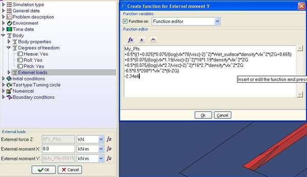
The software has been equipped with a new type of boundary condition in order to be capable of accounting for a pressurized free surface just like an aircushion. Figure 8 shows how the aforementioned aircushion model is easily implemented in the software interface.

Figure 8: Pressurized free surface implementation in SeaFEM interface.

4 Body dynamics

The ship dynamics consist of using Newton’s laws to obtain the ship movements once external loads acting on it are known. In this work, it is assume that the ship trajectory is fixed in the horizontal plane, constraining the surge, sway and yaw movements. On the other hand, heave, roll, and pitch will be free.

(25)

where ${\overline {\overline {\boldsymbol {M}}}}$ is the mass matrix, ${\overline {\overline {\boldsymbol {K}}}}$ is the restoring matrix, and ${\boldsymbol {F}}$ represents all kind of external forces and moments. Eq. (25) can be written as:

(26)

The equation of motions, Eq.(26), are solved using the well known Newmark´s scheme with parameters $\beta =1/4$ and $\gamma =1/2$ (also known as the average acceleration method).

{\begin{array}{c}{\boldsymbol {\dot {x}}}^{n+1}={\boldsymbol {\dot {x}}}^{n}+\Delta t{\frac {{\boldsymbol {\ddot {x}}}^{n+1}+{\boldsymbol {\ddot {x}}}^{n}}{2}}\\{\boldsymbol {x}}^{n+1}={\boldsymbol {x}}^{n}+\Delta t{\boldsymbol {\dot {x}}}^{n}+{\frac {\Delta t^{2}}{2}}{\frac {{\boldsymbol {\ddot {x}}}^{n+1}+{\boldsymbol {\ddot {x}}}^{n}}{2}}\end{array}}

(27)

When solving the body dynamics, care must be taken since not all loads are considered by default. Therefore, all those that are not considered by default, must be introduced externally via the available function editor for external forces and moments. By default, it is accounted for the weight and the buoyancy of the body, the hydrostatic restoring forces and moments, and the dynamic pressure integration over the wet surfaces. Any other loads, like those induced by the aircushion must be introduced manually via de function editor. Figure 9 shows an example of how external pitching moments are introduced within the interface. The aircushion pitching moment, for instance, is accessible via the My_Pfs variable. A wide range of internal variables are accessible for the function editor, which allows the implementation of a wide range of analytical models.

Figure 9: Introduction of external loads in SeaFEM

5 Structural solver

For the analysis of the flexible seals, two different alternatives were considered. First, to finish the development of a new rotation-free shell triangle [2] that holds the promise of avoiding numerical locking for very thin shells while maintaining accuracy. Second, to use an already developed membrane triangle [3].

The development of the shell element in the non-linear regime progressed more slowly than expected, and did not reach a sufficient mature status before the end of the project. Therefore, the focus turned towards the membrane solver.

The preference was set rather in favour of the shell element because for a coupled problem of this nature, an implicit solver is preferred. And for this, it is known that membrane solvers usually suffer from singularities in the system matrix.

Nevertheless, the membrane element has finally been used (in an implicit scheme), as it is expected to perform well at least in the modelling of the stern seals that are mostly subjected to tension state stress. The membrane solver uses a total Lagrangian formulation and assumes a linear-elastic behaviour of the material. The kinematic description is formulated in large displacements and large deformations, making use of the right Cauchy-Green deformation tensor. For further reference, see the reference [3].

The loads on the membrane are of two types. First, let’s consider the loads imposed by the air cushion system. The air cushion system acts differently on the bow skirt and the stern seal. On the bow skirt, the air cushion applies a direct follower load on the inner side of the skirt. On the stern seal, a differential pressure between the inside of the lobes and the air cushion maintains the seals taut. All these loads are considered as follower loads. A follower load has the property of not maintaining the symmetry of the system matrix for the implicit solver. Therefore, we need to choose an adequate numerical solver for the system of equations.

Second, the loads applied by the water by means of the interaction algorithm. The structural solver has been modified in order to consider the loads applied by the liquid as follower loads. Failing to include this consideration makes the system as a whole to diverge.

The contacts between the bow skirt stiffeners have been modelled as elastic contacts. This allows for a more realistic behaviour than considering the stiffeners stitched together and at the same time keeps the computational cost controlled.

6. Analyses of the XR-1B Surface Effect Ship

6.1 SES definition

First of all, let’s define the local frame of reference to be used. Figure 10 explains the location of the frame of reference used. The origin of coordinates is located at the intersection of the middle plane, the plane of the transom stern, and the water plane.

Figure 10: Local axis system definition

The XR-1B surface effect ship is used for this demonstration analysis. Figure 11 shows the geometry of the SES, and Table 1 provides information regarding the particular of the ship, as well as of the design conditions.

Figure 11: XR-1B geometry

Table 1: Particulars for the XR-1B

Length overall (m)	76.35
Length waterline on cushion (m)	67.52
Draft on cushion (m)	1.33
Beam max. (m)	22.25
Cushion width (m)	16.50
Cushion length (m)	67.14
Displacement (tonnes)	1560
LCG from wet deck transom (m)	33.75
TCG from starboard of centreline (m)	0
VCG above water line (m)	2.3564
Pitch gyradius (m)	21.6
Roll gyradius (m)	8.01
Aircushion average pressure (KPa)	11
Water depth (m)	10

6.2 Aircushion modelling

In order to carry out simulations, an aircushion model is needed. In this work, we will adopt an analytical aircushion model of the type [4]:

{\begin{array}{c}P^{ac}({\boldsymbol {x}},t)=P_{ave}\cdot {\mbox{0}}{\mbox{.25}}\cdot \left[{\mbox{tanh}}\left({\mbox{50}}\left({\frac {\mbox{x-37}}{\mbox{65}}}{\mbox{+0}}{\mbox{.5}}\right)\right){\mbox{-tanh}}\left({\mbox{100}}\left({\frac {\mbox{x-37}}{\mbox{60}}}{\mbox{-0}}{\mbox{.5}}\right)\right)\right]\\{\mbox{ }}{\mbox{ }}{\mbox{ }}{\mbox{ }}{\mbox{ }}{\mbox{ }}\cdot \left[{\mbox{tanh}}\left({\mbox{10}}\left({\frac {\mbox{y}}{\mbox{16}}}{\mbox{+0}}{\mbox{.5}}\right)\right){\mbox{-tanh}}\left({\mbox{10}}\left({\frac {\mbox{y}}{\mbox{16}}}{\mbox{-0}}{\mbox{.5}}\right)\right)\right]\end{array}}

(28)

The above pressure distribution accounts for a smooth pressure drop in the areas of the seals as well as when getting closer to the hull. Figure 12 shows the effect of the aircushion pressure on the free surface at zero speed.

Figure 12: Free surface drop due to aircushion pressure at Fr=0.

Let’s mention that the use of this specific aircushion is arbitrary, and results will highly depend on how well modelled the aircushion is. However, for the purpose of this demonstration, this arbitrary model is good enough since the purpose is to show how to use the tools developed, rather than modelling a specific real case. This model could be easily improved by using any experimental data of pressure distribution as well as pressure variations along with its governing equations. Should the aircushion behaviour be better known, then a better model could be implemented in the code. However, no realistic and verified model has been developed yet.

6.3 Dynamic model

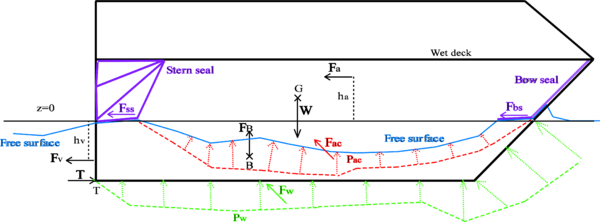
A number of forces are acting simultaneously when a surface effect ship is navigating. Figure 13 shows these forces. A brief description of each component is given next:

Weight ( ${\textstyle {\boldsymbol {W}}}$ ): is the ship weight.

Buoyancy ( ${\textstyle {\boldsymbol {B}}}$ ): resulting from hydrostatic pressure. Variations of this force due to ship positioning will be taken into account through the hydrostatic restoring matrix ${\textstyle {\overline {\overline {\boldsymbol {K}}}}}$ .

Viscous drag ( ${\textstyle {\boldsymbol {F}}_{v}}$ ): will be estimated following ITTC directions using the ITTC friction line. It will be assume to be horizontal and producing a pitching moment: ${\textstyle M_{y}^{v}=-F_{vx}\cdot (ZG-h_{v})}$ .

Wave making loads ( ${\textstyle {\boldsymbol {F}}_{w}}$ ): they are obtained by integrating the hydrodynamic pressure over the hulls.

Aircushion wave making loads ( ${\textstyle {\boldsymbol {F}}_{ac}}$ ): they are obtained by Eq.(23).

Bow seal drag ( ${\textstyle {\boldsymbol {F}}_{bs}}$ ) and stern seal drag ( ${\textstyle {\boldsymbol {F}}_{ss}}$ ): seal drags are mainly due to frictional forces. However, the amount of wet surface of the seal requires of solving a complex free surface-structure interaction problem where dynamic pressures over the seal are to be solved in order to determine the shape of the seal. The ITTC friction line will be used for estimating seal drags assuming a certain wetted area.

Aerodynamic profile drag ( ${\textstyle {\boldsymbol {F}}_{a}}$ ) : due to air pressure over the dry surfaces of the ship. It will be estimated as ${\textstyle {\boldsymbol {F}}_{a}={\frac {1}{2}}C_{a}S_{a}{\rho }_{a}v^{2}}$ ., where ${\textstyle C_{a}}$ is an aerodynamic coefficient usually obtained from model test, ${\textstyle S_{a}}$ is the frontal projected area, ${\textstyle {\rho }_{a}}$ is the air density, and ${\textstyle v}$ is the ship speed [5]. ${\textstyle {\boldsymbol {F}}_{a}}$ will be assumed to be horizontal. Then, it will induce a pitching moment as $M_{y}^{a}=-F_{x}(ZG-h_{a})$

Thrust ( ${\textstyle {\boldsymbol {T}}}$ ): provided by the propulsion system to compensate the drag forces. In this work, it will be taken as the sum of all drags: ${\textstyle T_{x}=-\left(F_{vx}+F_{wx}+F_{acx}+F_{bsx}+F_{ssx}+F_{ax}\right)}$ . It will be assume to be acting from the intersection of the base line with the transom stern, and to be horizontal. Then, this thrust will induce a pitching moment $M_{y}^{T}=-T_{x}(ZG+1.33)$ , where 1.33 stands for the draft.

More complex model can be found in the literature to model some of the previously described loads. Also, there are other external loads acting over a surface effect ship, such that aerodynamic momentum drag, air-leakage drag, and others [5]. However, for the sake of simplicity and for the demonstration purpose of this work, there is no need of including them in the analyses. In case of including them, they should be estimated in a reliable manner, which is out of the scope of this work. On the other hand, we will pay special attention to the estimation of the aircushion wave making loads and the loads resulting from the free-surface seal interaction, which are the main objectives of this work.

Figure 13: Forces acting over a surface effect ship

6.4 Wave drag induced by pressure patch

Moving pressurized free surface results in a wave train. Therefore, since some energy has been transferred to the fluid in the form of waves, a drag must be induced in the opposite direction to the movement of the pressurized free surface. This drag can be obtained via integration of the pressure distribution (excess of pressure over the atmospheric pressure) over the free surface. In case that the pressurize free surface is created by an ACV, the forces and moments acting over the ship are obtained via Eq.(23). Being capable of measuring these loads is a key point in the design of ACVs, and one of the main objectives of this work.

In [6] analytical solutions are found for the drag induced by several pressure distribution moving with constant forward speed in a canal. These solutions are linear and based on the Kelvin linearization. Figure 14 compares the wave drag coefficient induced by a rectangular pressure distribution (LxB) obtained by the proposed methodology versus the analytical solution provided in [6]. It can be observed that numerical results agree quite well overall.

Figure 14: Wave drag induced by uniform and rectangular pressure distribution in infinite depth and infinite width canal. L/B stands for length to beam ratio.

The lower the Froude number ${\textstyle v/{\sqrt {gL}}}$ (or the higher the dimensionless number ${\textstyle {\sqrt {{\frac {1}{2}}gL/v^{2}}}={\left({\sqrt {2}}Fr\right)}^{-1}}$ ), the higher are the difference between the numerical and analytical solutions. This discrepancy is not surprising since the waves generated by a pressure patch becomes more non-linear at lower Froude numbers [4], leading to more complex flows to be solved numerically. In fact, the lower the Froude number, the more complicated is obtaining a steady solution. In particular, at Froude number equal to 0.2, an unsteady wave is generated at the stern edge of the pressure patch. This wave moves back and forward in time, following an unsteady, but cyclical, process where at some times the wave becomes too steep to be solved under the numerical approach of this work. This steep wave generates some numerical dispersion that dissipates afterwards while the wave starts smoothing out till the cycle starts over. Despite of the limitations of the numerical approach used in here, it is capable of predicting the happening of these physical unstabilities, which might be critical in the design of ACVs.

6.5 Numerical towing test of the XR-1B

In this section, a first analysis on the XR-1B navigation properties will be carried out. In a first step, numerical simulations of the XR-1B with forward speed and all its degrees of freedom constraint are carried out. The main objective of these simulations is to obtain the loads induced by the dynamic pressure of the water over the hull as well as by the aircushion. All the other loads are either known or estimated via analytical models. Table 2 shows the drag, vertical forces and pitching moments

Table 2: Wave making and aircushion loads

	Dynamic pressure loads			Aircushion loads
${\mbox{Fr}}$	${\mbox{Fw}}_{\mbox{X}}{\mbox{ (N)}}$	${\mbox{Fw}}_{\mbox{Z}}{\mbox{ (N)}}$	${\mbox{Mw}}_{\mbox{Y}}{\mbox{ (Nm)}}$	${\mbox{Fac}}_{\mbox{X}}{\mbox{ (N)}}$	${\mbox{Fac}}_{\mbox{Z}}{\mbox{ (N)}}$	${\mbox{Mac}}_{\mbox{Y}}{\mbox{ (Nm)}}$
0	0	0	0	0	10388780	-20660000
0.1	-50200	220000	600000	-70000	10388780	-20550000
0.2	-60000	250000	2800000	-280000	10388780	-19900000
0.3	-66000	-1010000	-1270000	-220000	10388780	-20135800
0.4	-112400	-1320000	-33550000	-503600	10388780	-19407100
0.6	-95810	533400	-26000000	-282390	10388780	-19834520
0.8	-117594	1059660	-12136880	-276460	10388780	-19816880
1.2	-178965	1447142	3634880	-183518	10388780	-20142400
1.6	-260156	1545982	14873440	-116532	10388780	-20354600
2	-358270	1480790	22941400	-76991	10388780	-20468000

6.6 Viscous loads

The viscous drag ${\textstyle {\boldsymbol {F}}_{v}}$ will be estimated following ITTC directions using the ITTC friction line.

(29)

where $C_{v}={\boldsymbol {F}}_{v}/({\frac {1}{2}}{\rho }_{w}Sv^{2})$ is the dimensionless viscous drag coefficient, ${\rho }_{w}=1025kg/m^{3}$ is the fluid density, ${\textstyle S=617.3{\mbox{ }}m^{2}}$ is the wet surface, and ${\textstyle k}$ is the form factor which, for this demonstration, will be assumed to be equal to 0.025. ${\textstyle {\boldsymbol {F}}_{v}}$ will be assumed to be horizontal and located at a height of ${\textstyle h_{v}={\mbox{-0}}{\mbox{.665}}{\mbox{ }}{\mbox{m}}}$ . Then, the viscous load will induce a pitching moment $Mv_{Y}=-Fv_{X}\cdot (ZG-h_{v})$ .

6.7 Seal loads

The seal loads are mainly frictional loads. In this first approximation, we will estimate using the ITTC viscous drag coefficient. The wet surface is estimated as ${\textstyle S=B\cdot l}$ , where ${\textstyle B}$ is the aircushion width, and ${\textstyle l}$ is the wet length of the seal. The wet length for the bow and stern seals will be assumed to be ${\textstyle l_{bs}=1.19{\mbox{ }}m}$ and ${\textstyle l_{ss}=2.7{\mbox{ }}m}$ respectively. Both frictional forces will be assumed to be horizontal and acting on the z=0 plane. Therefore, they will induce a pitching moment $Ms_{Y}=-Fs_{X}\cdot ZG$ .

Table 3: Hull viscous loads

${\mbox{Fr}}$	${\mbox{Re}}$	${\mbox{C}}_{\mbox{v}}$	${\mbox{Fv}}_{\mbox{X}}{\mbox{ (N)}}$	${\mbox{Fv}}_{\mbox{Z}}{\mbox{ (N)}}$	${\mbox{Mv}}_{\mbox{Y}}{\mbox{ (Nm)}}$
0	0	0	0	0	0
0.1	1.75 10⁸	1.972 10^-3	-3900	0	11783
0.2	3.5 10⁸	1.795 10^-3	-14197	0	42894
0.3	5.25 10⁸	1.702 10^-3	-30291	0	91521
0.4	7 10⁸	1.641 10^-3	-51903	0	156819
0.6	1.05 10⁹	1.559 10^-3	-110997	0	335365
0.8	1.4 10⁹	1.505 10^-3	-190488	0	575540
1.2	2.1 10⁹	1.434 10^-3	-408231	0	1233428
1.6	2.8 10⁹	1.386 10^-3	-701596	0	2119804
2	3.5 10⁹	1.351 10^-3	-1068261	0	3227644

Table 4: Bow Seal loads

${\mbox{Fr}}$	${\mbox{Re}}$	${\mbox{C}}_{\mbox{v}}$	${\mbox{Fbs}}_{\mbox{X}}{\mbox{ (N)}}$	${\mbox{Fbs}}_{\mbox{Z}}{\mbox{ (N)}}$	${\mbox{Mbs}}_{\mbox{Y}}{\mbox{ (Nm)}}$
0	0	0	0	0	0
0.1	2.98 10⁶	3.75 10^-3	-2.36E+02	0.00E+00	5.55E+02
0.2	5.95 10⁶	3.29 10^-3	-8.28E+02	0.00E+00	1.95E+03
0.3	8.93 10⁶	3.06 10^-3	-1.73E+03	0.00E+00	4.08E+03
0.4	1.19 10⁷	2.91 10^-3	-2.93E+03	0.00E+00	6.90E+03
0.6	1.79 10⁷	2.72 10^-3	-6.16E+03	0.00E+00	1.45E+04
0.8	2.38 10⁷	2.59 10^-3	-1.04E+04	0.00E+00	2.46E+04
1.2	3.57 10⁷	2.43 10^-3	-2.20E+04	0.00E+00	5.19E+04
1.6	4.76 10⁷	2.33 10^-3	-3.75E+04	0.00E+00	8.83E+04
2	5.95 10⁷	2.25 10^-3	-5.66E+04	0.00E+00	1.33E+05

Table 5: Stern Seal loads

${\mbox{Fr}}$	${\mbox{Re}}$	${\mbox{C}}_{\mbox{v}}$	${\mbox{Fss}}_{\mbox{X}}{\mbox{ (N)}}$	${\mbox{Fss}}_{\mbox{Z}}{\mbox{ (N)}}$	${\mbox{Mss}}_{\mbox{Y}}{\mbox{ (Nm)}}$
0	0	0	0	0	0
0.1	6.75 10⁶	3.22 10^-3	-4.59E+02	0.00E+00	1.08E+03
0.2	1.35 10⁷	2.85 10^-3	-1.63E+03	0.00E+00	3.83E+03
0.3	2.03 10⁷	2.66 10^-3	-3.42E+03	0.00E+00	8.06E+03
0.4	2.7 10⁷	2.54 10^-3	-5.81E+03	0.00E+00	1.37E+04
0.6	4.05 10⁷	2.39 10^-3	-1.23E+04	0.00E+00	2.89E+04
0.8	5.4 10⁷	2.28 10^-3	-2.08E+04	0.00E+00	4.91E+04
1.2	8.1 10⁷	2.15 10^-3	-4.41E+04	0.00E+00	1.04E+05
1.6	1.08 10⁸	2.06 10^-3	-7.53E+04	0.00E+00	1.77E+05
2	1.35 10⁸	2 10^-3	-1.14E+05	0.00E+00	2.68E+05

6.8 Air profile loads

The aerodynamic profile drag ${\textstyle {\boldsymbol {F}}_{a}}$ will be estimated as ${\textstyle {\boldsymbol {F}}_{a}={\frac {1}{2}}C_{a}S_{a}{\rho }_{a}v^{2}}$ . We will assume a projected area ${\textstyle S_{a}=200{\mbox{ }}m^{2}}$ , and a drag coefficient of ${\textstyle C_{a}=0.5}$ . ${\textstyle {\boldsymbol {F}}_{a}}$ will be assumed to be horizontal and located at $h_{a}=6m$ . Therefore, the induced pitching moment is $M_{y}^{a}=-F_{x}(ZG-h_{a})$ .

Table 6: Air profile loads

${\mbox{Fr}}$	${\mbox{Fa}}_{\mbox{X}}{\mbox{ (N)}}$	${\mbox{Fa}}_{\mbox{Z}}{\mbox{ (N)}}$	${\mbox{Ma}}_{\mbox{Y}}{\mbox{ (Nm)}}$
0	0	0	0
0.1	-313	0	-1139
0.2	-1250	0	-4555
0.3	-2813	0	-10248
0.4	-5000	0	-18218
0.6	-11250	0	-40991
0.8	-20000	0	-72872
1.2	-45000	0	-163962
1.6	-80000	0	-291488
2	-125000	0	-455450

6.9 Propulsion

The propulsion system has to provide the thrust required to compensate the drag. Therefore, the horizontal thrust to be provided can be estimated by summing up all the drags given above. We will assume a propulsion system to be equivalent to an horizontal force (thrust) acting on the intersection of the base line and the stern, that is to say, acting at (XE, YE, ZE)=(0,0,-1.33). Then, the propulsion system will induce a pitching moment of

Table 7: Propulsion loads

${\mbox{Fr}}$	${\mbox{Ft}}_{\mbox{X}}{\mbox{ (N)}}$	${\mbox{Ft}}_{\mbox{Z}}{\mbox{ (N)}}$	${\mbox{Mt}}_{\mbox{Y}}{\mbox{ (Nm)}}$
0	0	0	0
0.1	125107	0	-461194
0.2	357901	0	-1319366
0.3	324256	0	-1195338
0.4	681637	0	-2512787
0.6	518857	0	-1912715
0.8	635830	0	-2343923
1.2	881890	0	-3251001
1.6	1271010	0	-4685453
2	1799020	0	-6631907

6.10 Drag prediction

Figure 15 and Figure 16 show the estimated drag components and cumulative drag respectively. It can be observed that the aircushion drag is especially important at lower Froude numbers. However, as the Froude number increases, frictional drag of the hulls becomes dominant, followed by wave making and seal drags, while the aircushion drag becomes less important.

6.11 Sink and trim

In order to obtain the equilibrium position (sinkage and trimming angle), of the XR-1B for each velocity condition, Eq. (25) must be solved in the absence of the inertial term:

(30)

In order to obtain the equilibrium sinkage and trimming when the XR-1B is moving forward in the absence of waves, it is necessary to know the vertical forces and pitching moments acting on the ship, as well as the hydrostatic properties of the ship. Figure 17 and Figure 18 shows the vertical forces and pitching moments at different Froude numbers, and Table 8 provides the hydrostatic properties.

Table 8: Hydrostatic coefficients for the XR-1B

${\mbox{B(T)}}$	${\mbox{348}}{\mbox{.447}}$
${\mbox{X}}_{\mbox{B}}{\mbox{(m)}}$	${\mbox{31}}{\mbox{.78}}$
${\mbox{Y}}_{\mbox{B}}({\mbox{m)}}$	$0$
${\mbox{Z}}_{\mbox{B}}{\mbox{(m)}}$	${\mbox{-0}}{\mbox{.545}}$
${\textstyle {\mbox{K}}_{\mbox{33}}({\mbox{N/m}})}$	${\textstyle {\mbox{3}}{\mbox{.58234}}\cdot {\mbox{10}}^{\mbox{6}}}$
${\textstyle {\mbox{K}}_{\mbox{34}}({\mbox{N/rad}})}$	${\textstyle 0}$
${\textstyle {\mbox{K}}_{\mbox{35}}({\mbox{N/rad}})}$	${\textstyle {\mbox{6}}{\mbox{.33958}}\cdot {\mbox{10}}^{\mbox{6}}}$
${\textstyle {\mbox{K}}_{\mbox{44}}({\mbox{Nm/rad}})}$	${\textstyle {\mbox{3}}{\mbox{.22157}}\cdot {\mbox{10}}^{\mbox{8}}}$
${\textstyle {\mbox{K}}_{\mbox{45}}({\mbox{Nm/rad}})}$	${\textstyle 0}$
${\textstyle {\mbox{K}}_{\mbox{46}}({\mbox{Nm/rad)}}}$	${\textstyle {\mbox{6}}{\mbox{.72248}}\cdot {\mbox{10}}^{\mbox{6}}}$
${\textstyle {\mbox{K}}_{\mbox{55}}({\mbox{Nm/rad}})}$	${\textstyle {\mbox{1}}{\mbox{.25383}}\cdot {\mbox{10}}^{\mbox{9}}}$
${\textstyle {\mbox{K}}_{\mbox{56}}({\mbox{Nm/rad)}}}$	${\textstyle 0}$

Notice that based on the local reference system of the XR-1B, negative pitch moments induce sinkage of the bow and negative values of the pitch angle. However, we will say that the trim angle is negative when it induces the sinkage of the bow. That is to say, the trim angle is the pitch angle but in opposite direction.

Solving Eq. (30) for the loads estimated above, we obtain the sinkage and trimming for each Froude number. Figure 19 and Figure 20 Shows the evolution of sinkage and trimming across a range of Froude numbers.

6.12 XR-1B in regular waves

A set of numerical tests for a range of wave periods and wave directions have been carried out for Fr=1.6 and forward speed. The aim of these tests is to estimate response amplitude operators (RAOs) in heave, roll and pitch, so that complicated navigating conditions could be anticipated. The wave direction is measured respect to the OX axis and positive clockwise. That is to say, a direction of 180º means head seas, while 0º means following seas.

Figure 30, Figure 31, and Figure 32 provide the results from the numerical test. It can be observed that stern quartering waves with wave periods around 9s-10s are the most dangerous ones out of the range analyzed. Strong resonance effect might appear leading to an unstable behaviour of the ship.

Figure 15: XR-1B drag components

Figure 16: XR-1B cumulative drag

Figure 17: Vertical forces induced on the XR-1B .

Figure 18: Pitching moments induced on the XR-1B .

Figure 19: Sinkage.

Figure 20: Trim.

Figure 21: Wave pattern at Froude number 0.1

Figure 22: Wave pattern at Froude number 0.2

Figure 23: Wave pattern at Froude number 0.3

Figure 24: Wave pattern at Froude number 0.4

Figure 25: Wave pattern at Froude number 0.6

Figure 26: Wave pattern at Froude number 0.8

Figure 27: Wave pattern at Froude number 1.2

Figure 28: Wave pattern at Froude number 1.6

Figure 29: Wave pattern at Froude number 2

Figure 30: Response amplitude operator in heave for XR-1B in waves at Fr=1.6

Figure 31: Response amplitude operator in roll for XR-1B in waves at Fr=1.6

Figure 32: Response amplitude operator in pitch for XR-1B in waves at Fr=1.6

6.13 High speed manoeuvring of the XR-1B in still water

In order to assess the manoeuvring capabilities of the XR-1B, a set of test runs performing a turning circle have been carried out at Fr=1.6. The test runs have been performed in different conditions, based on the depth, turning diameter and drift angle (see Figure 33).

Figure 33: Turning circle manoeuvre definition

The aim of this test is threefold: First, to evaluate the seakeeping behaviour while manoeuvring at different turn diameters; second, to evaluate the influence of the water depth; and third, to evaluate the influence of the drift angle of the ship.Figure 34, Figure 35, and Figure 36 show the wave pattern for a turn with D=700m for each test.

Table 9 contains the seakeeping results obtained. While no big differences are observed between conditions 1 and 2, big differences are observed from these ones with respect to condition 3. The effect of the drift basically consists of introducing a side slip velocity. This side slip velocity, which is in the order of 9% of the forward speed for a 5º drift, highly modifies the flow field around the ship, inducing a much different dynamic pressure distribution which induces larger movements.

Figure 34: XR-1B performing a turn of D=700m. Water depth: 10m. Drift angle=0º.

Figure 35: XR-1B performing a turn of D=700m. Water depth: 100m. Drift angle=0º.

Figure 36: XR-1B performing a turn of D=700m. Water depth: 100m. Drift angle=5º.

Table 9: Turning circle seakeeping results.

D (m)	Condition 1				Condition 2				Condition 3
	H=10m		Drift=0º		H=100m		Drift=0º		H=10m		Drift=5º
	Heave (m)	Roll (º)		Pitch (º)	Heave (m)	Roll (º)		Pitch (º)	Heave (m)	Roll (º)		Pitch (º)
300	-0.948	2.509		-0.320	-1.031	2.419		-0.406	-5.059	4.815		12.694
350	-0.671	1.995		-0.323	-0.739	1.912		-0.414	-2.483	2.426		-0.683
400	-0.495	1.626		-0.311	-0.556	1.552		-0.409	-1.183	1.469		-7.848
500	-0.289	1.178		-0.254	-0.346	1.123		-0.360	-0.109	0.854		-14.227
700	-0.123	0.800		-0.206	-0.177	0.762		-0.309	0.416	0.767		-17.768
1000	-0.033	0.519		-0.158	-0.087	0.499		-0.281	0.491	0.943		-18.593
inf	0.033	0		-0.118	-0.020	0		-0.299	-0.166	1.471		-15.642

Table 10: Turning circle pressure loads

D (m)	Condition 1				Condition 2				Condition 3
	H=10m		Drift=0º		H=100m		Drift=0º		H=10m		Drift=5º
	Fx (T)	Fy (T)		Mz (Tm)	Fx (T)	Fy (T)		Mz (Tm)	Fx (T)	Fy (T)		Mz (Tm)
300	-21.51	-10.20		7158.41	-21.16	-13.36		7107.42	-16.74	773.62		34686.36
350	-23.32	-30.59		6118.30	-23.10	-32.75		6061.19	-20.86	399.02		22224.31
400	-24.47	-41.50		5384.10	-24.34	-42.76		5322.92	-23.17	207.17		14727.86
500	-26.00	-42.93		4252.22	-25.88	-43.34		4181.86	-25.45	53.33		7389.40
700	-27.23	-32.79		2907.50	-27.12	-32.94		2856.23	-26.92	-21.30		2419.15
1000	-27.94	-24.17		1998.64	-27.87	-24.33		1967.03	-27.46	-48.52		-101.42
inf	-28.55	0		0	-28.45	0		0	-27.07	-119.67		-6029.33

Table 11: Turning circle aircushion loads

D (m)	Condition 1				Condition 2				Condition 3
	H=10m		Drift=0º		H=100m		Drift=0º		H=10m		Drift=5º
	Fx (T)	Fy (T)		Mz (Tm)	Fx (T)	Fy (T)		Mz (Tm)	Fx (T)	Fy (T)		Mz (Tm)
300	-23.43	-16.01		-2477.91	-26.48	-15.19		-2487.09	-41.29	-131.95		-9969.88
350	-20.36	-4.39		-2173.66	-23.56	-3.61		-2364.72	-30.98	-77.17		-6812.31
400	-18.15	2.74		-1951.13	-21.44	3.47		-1956.84	-24.47	-48.28		-4871.71
500	-15.50	7.61		-1599.48	-18.94	8.15		-1600.95	-18.05	-19.44		-2815.15
700	-13.66	7.16		-1121.69	-17.19	7.49		-1122.71	-13.95	2.56		-1130.23
1000	-12.64	5.96		-780.08	-16.23	6.16		-781.10	-13.02	15.74		-87.01
inf	11.80	1.01		-8.71	-15.46	0.77		-6.44	-14.31	36.66		2070.12

6.14 High speed manoeuvring of the XR-1B in low seas

Looking at Figure 30, Figure 31, and Figure 32, unstable behaviour can be expected when navigating at high speeds, leading to the incapability of navigating with waves. On the other hand, still water result might not be that useful since they don’t take into account the effect that there always are small waves that might work as small perturbation that might excite large movements in a SES.

A seakeeping test run has been carried out to simulate the performance of the XR-1B when performing a turn of tactical diameter D=700m in TD=55s (Fr=1.6). The manoeuvre is performed in the presence of small waves corresponding to a Pierson Moskowitz spectrum with significant wave height of 0.1 meter and mean period of 9 seconds. Figure 37, Figure 38, and Figure 39 show the heave, roll and pitch motion obtained during the simulation. At the beginning of the turn, waves propagate as following seas and covering an angular sector of 30º.

Figure 37: XR-1B heave motion at high Speed when performing a turn in low seas.

Figure 38: XR-1B roll motion at high Speed when performing a turn in low seas.

Figure 39: XR-1B pitch motion at high Speed when performing a turn in low seas.

6.15 Very shallow water effect

This section aims at showing the effect of navigating in shallow waters. The XR-1B have been simulated navigating at 10m/s (Fr=0.4 approx.) in three different water depths of 2.216 m, 10 m, and 100m. Figure 40, Figure 41, and Figure 42 show the wave pattern for each water depth.

Figure 40: Wave pattern at Fr=0.4 and 100 meters depth.

Figure 41: Wave pattern at Fr=0.4 and 10 meters depth.

Figure 42: Wave pattern at Fr=0.4 and 2.216 meters depth.

Table 12 compares drag, lifting force and pitching moment induced by the hydrodynamic pressure field over the hulls and by the aircushion.

Table 12: Loads induced by hydrodynamic pressure and air cushion loads at Fr=0.4 and different water depths.

Depth (m)		2.216	10	100
Hydrodynamic pressure	Fx (T)	8.12	11.46	8.39
	Fz (T)	83.21	-134.60	-28.55
	My (Tm)	-4625.43	-3421.15	1693.75
Air cushion	Fx (T)	27.02	51.35	26.83
	Fz (T)	1059.36	1059.36	1059.36
	My (Tm)	-37851.87	-1978.97	-37841.67

As expected, the drag and sinkage are larger at shallow water depths than at infinite or very shallow waters. Regarding the pitching moment, it is dominated by the aircushion, resulting in a big reduction of its pitch moment at shallow waters, leading to the immersion of the bow.

6.16 Free surface-seal interaction

In this section, a set of test runs are performed for the XR-1B with rigid seals. Rigid seals behave as planning surfaces when in contact with the free surface. Therefore, a free surface rising in the front face of the seal is expected, as well as a pressure profile with a peak pressure where the free surface impacts the seal. Hydrodynamic pressure integration over the wet surface of the seals will provide the forces and moments induced on the XR-1B. It will be showed that these forces and moments induced by rigid seals working as planning surfaces are much bigger than the actual forces and moments obtained in reality, and therefore, rigid seals shouldn’t be assumed to be a good approximation for flexible seals. Moreover, the shape of the rigid seal must be guest beforehand to approximate the final shape of the flexible seals in steady conditions, which is quite unpredictable and depends on many working conditions.

6.16.1 Rigid bow seals

Despite of considering that rigid seals are not a realistic approximation for a real SES, the main reason to carry out these set of tests is to prove the validity of the free surface-seal interaction algorithm explained in section 2.2.4. This algorithm is a key point in order to solve the free surface and flexible seals interaction, since the pressure field obtained via this algorithm will feed the structural solver that will analyze how the seals will deform, and will feed-back the new shape of the seal to the algorithm.

In this section, we will analyze two types of bow seals, called plate and fingers. The former is assumed to be a flat plate when undeflected, while the latter is assumed to have the typical finger shape used in bow seals. In both cases, the seal is assumed to be undeflected (linear) in the dry (upper) side, and deflected in the wet (lower) side. The deflection in the wet side is assumed to be cubic and to fulfil tangency condition with the undeflected side, as well as horizontal tangency at the lower end. This ad-hoc deflection of the bow seal has been adopted based on [7].

However, this model required of a guess of when the transition from the wet to the dry side will happen. As shown in Figure 43: the water level has been assumed to rise up to 1 meter in height. It is shown next that this estimation is quite close for high Froude numbers, when the seal is behaving as a planning surface.

Figure 43: Geometrical description of bow and stern rigid seals.

Figure 45 shows the dimensionless pressure distribution obtained in a mid section of the flat plate bow seal. For the lower Froude number, Fr=0.2, the water impact the seal around x=68, which corresponds to a water raise of about 0.8 meters (based on Figure 45). For Fr=0.4, the water impact moves forward up to 68.7 m, corresponding to a water raise over 1.5 meters. On the other hand, as the Froude number increases, the water impact stays very stable around x=68.25 m, corresponding to a water rise of 1 meter, as assumed beforehand. Also, for the higher Froude numbers, the dimensionless pressure distribution corresponds to a typical pressure distribution of a planning surface, reaching up to one right after the impact point, and decreasing to the reference free surface pressure towards the trailing edge.

Figure 44: Bow seal pressure for plate bow seals.

Figure 45: Dimensionless pressure distribution in the mid section of the plate bow seals.

6.16.2 Towing test with rigid seals

Towing tests in a range of Froude numbers have been simulated considering including the above mentioned rigid seals. The free surface-seal interaction algorithm has been used to simulate the planning surface behaviour of the seals. As a result, the free surface elevation and pressure field underneath the seals are obtained. Hydrodynamic pressure integration over the seals surfaces provide the forces and moments induced on the XR-1B. Table 13 shows the results obtained in the simulation.

Figure 46 shows the geometry of the XR-1B along with the rigid seal geometries used in the simulations. Figure 47 shows the pressure distribution resulting over the bow seal when the ship is moving with constant forward speed and restrained in movement.

Figure 46: Geometry of the XR-1B with rigid seals.

Table 13: Forces and moments induced by rigid seals on the XR-1B SES

Fr	Fx (N)	Fz (N)	My (Nm)
0	0	0	0
0.1	-9.15E+03	2.23E+04	-1.13E+05
0.2	-8.14E+04	1.64E+05	-3.42E+06
0.3	-1.97E+05	1.99E+05	-1.38E+07
0.4	-5.84E+05	5.27E+05	-3.71E+07
0.6	-1.52E+06	1.44E+06	-1.00E+08
0.8	-2.56E+06	2.52E+06	-1.75E+08
1.2	-5.68E+06	5.64E+06	-3.92E+08
1.6	-9.84E+06	9.92E+06	-6.87E+08
2	-1.55E+07	1.54E+07	-1.08E+09

Comparing the values in Table 13 with Table 4 and Table 5, it is observed that loads induced by rigid seals working as planning surfaces are much higher that those induced by viscous friction. Moreover, these loads are much higher than any other component as speed increases. Therefore, the use of rigid seals seems not to be appropriate for modelling flexible seals. Figure 47 shows the pressure field induced on the finger of the bow seal located in the port side. Negative pressures indicate areas where pressure drops below atmospheric pressure. The free surface at those nodes cannot detach unless it is surrounded by, at least, one detached node, allowing the entrance of air.


Fr=0.1	Fr=0.2

Fr=0.3	Fr=0.4

Fr=0.6	Fr=0.8

Fr=1.2	Fr=1.6

Fr=2

Figure 47: Pressure field induced over a rigid bow seal due to free surface-seal interaction in towing test. Only fingers located at the port side are shown.

It is important to understand that the high pressure induced in the seal should reshape the seal such that the pressure should drop to a value where dynamic equilibrium exists. Should this equilibrium be reached, the final shape of the seal would be found, and this shape should be parallel to the free surface. Then, based on the amount of wet surface of the seal and its final position, viscous friction could be estimated.

6.16.3 XR-1B in waves with rigid seals

In this section, the dynamics of the XR-1B SES is analyzed when in the presence of a regular wave and using rigid seals. While viscous drag, aerodynamic profile drag, and propulsion forces and moments are estimated using the previously used analytical models, forces and moments induced by the hydrodynamic pressure on the hull, aircushion pressure, and hydrodynamic pressure on the seals are calculated in the hydrodynamic solver and accounted for in the dynamic solver in each time step.

Since rigid seals behave as planning surfaces, they have a very large influence on the dynamics of the SES, and the higher the speed of the ship, the larger the influence. Therefore, the dynamics of a SES with rigid seals is not an appropriate model for a real SES with flexible skirts. However, it is a previous step aiming to analyze the free surface-seal interaction scheme proposed in this work.

Figure 48, Figure 49, and Figure 50 show the XR-1B motions for one hundred seconds when moving with forward speed in the presence of a regular wave. It is noticeable that as the speed increases, the movements of the ship become larger. These large movements are induced by the large pressure values obtained on the wet side of the rigid seals. These large pressure values are the result of the high speed of the craft in combination with the seals working as planning surfaces, which stagnates the flow around the impact area and increases the pressure up to the stagnation value.

Figure 51, Figure 52, and Figure 53 show the temporal variation of the forces and moments resulting from pressure integration over the rigid seals. Figure 54, Figure 55, and Figure 56 show snapshots of free surface elevation and pressure over seals.

Figure 48: Heave and pitch motions for XR-1B SES with rigid seas at Fr=0.4 and in the presence of a regular wave with H=0.5m and T=6s.

Figure 49: Heave and pitch motions for XR-1B SES with rigid seas at Fr=0.8 and in the presence of a regular wave with H=0.5m and T=6s.

Figure 50: Heave and pitch motions for XR-1B SES with rigid seas at Fr=1.6 and in the presence of a regular wave with H=0.5m and T=6s.

Figure 51: Drag induced by pressure integration on rigid seals in the presence of waves.

Figure 52: Lift induced by pressure integration on rigid seals in the presence of waves.

Figure 53: Pitching moment induced by pressure integration on rigid seals in the presence of waves.

Figure 54: Snapshots of XR-1B with rigid seals at Fr=0.4. From left to right: time=5s, time=10s, and time=15s. From top to bottom: free surface elevation, pressure over bow seal, pressure over stern seal.

Figure 55 : Snapshots of XR-1B with rigid seals at Fr=0.8. From left to right: time=5s, time=10s, and time=15s. From top to bottom: free surface elevation, pressure over bow seal, pressure over stern seal.

Figure 56 : Snapshots of XR-1B with rigid seals at Fr=1.6. From left to right: time=5s, time=10s, and time=15s. From top to bottom: free surface elevation, pressure over bow seal, pressure over stern seal.

6.17 Towing test with flexible seals

In this section, the behaviour of the seals of the XR-1B is analysed. Different types of simulations have been performed. On one hand, the effect of the flexible bow seals has been analysed. Afterwards bow and stern seals have been included in the analyses. The cushion model using in these tests is that presented in previous sections.

The fluid-structure interaction model used for these analyses has been described in sections 2.2.4 and 2.2.5. The ingredients of this model are the following:

A free surface solver, able to find a pressure field to be applied over the free surface such that the obtained is limited by the location of the seal. That is to say, the seal act as an upper limit for the free surface elevation. The free surface boundary conditions are applied in different ways depending on whether the free surface is in contact with the seal or not. If the free surface is not in contact, the boundary conditions are applied as if there is no seal, but if there is contact, the implementation will be different in order to ensure that the free surface does not penetrate de seal and the necessary pressure to fulfil this condition is calculated.

A dynamic FEM structural solver based on 3 nodes membrane elements, to model the seals deformation.

A staggered interaction algorithm: pressure field obtained from the above mentioned free surface solver is sent at the beginning of every time step to the dynamic structural solver. The obtained vertical displacements of the seals are sent back to the free surface solver, in order to compute the updated pressure field in the following time step.

A TCL interface, based on TCL sockets, able to communicate during execution and at memory levels both solvers. The interface includes an interpolation library used to perform the coupling. This interpolation library is capable of interpolating data (scalar or vectorial fields) from one mesh to another mesh. The meshes need not be matching, but should be discretizations of the same surface. The interpolation library was developed by Compass and is a general purpose C++ code provided for this project. The interaction is performed using a TCL script invoked from the hydrodynamics solver. This script uses the interpolation library to pass pressure information from the hydrodynamics mesh to the structural mesh, and vertical displacements from the structural mesh to the hydrodynamics mesh.

The seals structural models used in these analysis consisted on 12976 triangular membrane elements (6864 nodes) for the bow seal and 18608 elements (9428 nodes) for the stern seals.

The following pictures show the boundary conditions using in the structural model, for the bow seals. These include fixed constraints in upper part and non-linear elastic constraints in the sides of the seals. The later simulate the mechanic contacts of neighbouring fingers.


Figure 57. Fix constraints (left) and non-linear elastic constraints in bow seals (right).

The boundary conditions for the stern seal include fixed constraints in upper part and rigid boundary constraints. The later simulate the mechanic contact between the upper and lower lobe. The boundary conditions for the bow seal are shown in the following picture.


Figure 58. Fix constraints in stern seals (left) and Rigid boundary constraints in stern seals (right).

6.17.1 Analysis with flexible bow seals

In this section, the towing test of the craft is analysed, including flexible fingers (bow seals). Three velocities are run, Froude numbers 0.4, 0.8 and 1.2.

In the following sequences, the deformed bow seals, wave pattern and cushion free surface deformation for the different analyses are shown. In the different results, it can be seen how the seals interaction creates an unstable free surface deformation pattern in the cushion, for the higher Froude numbers, while the solution is quite steady for the smaller figure. In this latter case, the deformation of the seals is very small, since the dynamic pressure acting on the seals is quite similar to the cushion pressure.

It is important to remark that the seals deformation obtained for the higher speeds qualitatively agrees with the experimental information available. Unfortunately, no quantitative data exists to further validate these results.




Figure 59. Bow seals deformation sequence: t=2, 4, 6, 8, 10, 12 sec. (from left to right and top to bottom) for Fr=0.4.




Figure 60. Wave pattern and cushion free surface deformation sequence: t=2, 4, 6, 8, 10, 12 sec. (from left to right and top to bottom) for Fr=0.4.




Figure 61. Bow seals deformation sequence: t=1, 2, 3, 4, 5, 6 sec. (from left to right and top to bottom) for Fr=0.8.




Figure 62. Wave pattern and cushion free surface deformation sequence: t=1, 2, 3, 4, 5, 6 sec. (from left to right and top to bottom) for Fr=0.8.




Figure 63. Bow seals deformation sequence: t=1, 2, 3, 4, 5 sec. (from left to right and top to bottom) for Fr=1.2.




Figure 64. Wave pattern and cushion free surface deformation sequence: t=1, 2, 3, 4, 5 sec. (from left to right and top to bottom) for Fr=1.2.

6.17.2 Analysis with flexible bow and stern seals

In this section, the towing test of the craft is analysed, including flexible bow and stern seals for a Froude number of 1.2.

In the following sequences, the deformed bow and stern seals, wave pattern and cushion free surface deformation are shown. The results show how the bow seals create an unstable free surface deformation pattern in the cushion area, while the stern seal is deformed until it is adapted to a configuration in which it almost slides on the water.

Again, the bow seals deformation obtained qualitatively agrees with the experimental information available. With respect to this, figure 67 shows a comparison between the computed seal deformation and a picture obtained in a test, taken from reference [9].



Figure 65. Bow seals deformation sequence: t=1, 2, 3, 4 sec. (from left to right and top to bottom) for Fr=1.2.



Figure 66. Stern seals deformation sequence: t=1, 2, 3, 4 sec. (from left to right and top to bottom) for Fr=1.2.

Figure 67. Stern seals deformation sequence at 2.5 sec and test data obtained of Reference [9].



Figure 68. Wave pattern and cushion free surface deformation sequence: t=1, 2, 3, 4 sec. (from left to right and top to bottom) for Fr=1.2.

7. Particulars of the software

Some of the main concerns when carrying out computational fluid dynamics (CFD) simulations are the computational resources and time required. In our case study, the analysis of the seakeeping and manoeuvring capabilities of a surface effect ship is not an exception. On the contrary, it requires to simulate several complex phenomena coupled between them, such as wave making, aircushion dynamics, free surface-seal interaction, and ship dynamics.

Different approaches with different types of accuracy can be taken to cope with such an analysis. For instance, in [8], the semi-coupled two phase URANS CFD Ship-Iowa V4.5 is sued for evaluating the performance of the XR-1B SES. While the outcome of the analyses is outstanding, the CPU-time reported is quite unaffordable for being used systematically during design stages.

In this work, a potential flow approach along with first order Stokes waves and small movement approximation is used. While this approximation is much simpler than using RANS computations, significant outcomes can be obtained as well, allowing to significantly reducing computational time by 2 or 3 orders of magnitude even when computing on a regular desktop or laptop.

The use of potential flow requires the use of semi-analytical formulation in order to account for viscous effects, such as viscous drag and skin-friction drag in seals. On the other hand, the number of degrees of freedom is reduced from four, three 3 velocities components and pressure, to just one (the velocity potential). Moreover, having no need of modelling turbulence allows for having a much coarser discretization.

On the other hand, the use of the Stokes approximation for treating the free surface, along with small movements, leads to having fix boundary along the calculations, which reverberates in having high computational savings.

Despite of starting off with lesser computational requirements than more complex approaches like in [8], special attention has been paid to reducing CPU-time. Looking at the computational time of different part of the code, it was realized that most computational effort was spent in the linear solver. Therefore, the main objective towards reducing computational time has been oriented to accelerating the iterative solver.

7.1 Iterative solver acceleration

Some iterative solvers such as preconditioned conjugate gradient and preconditioned bi-conjugate gradient failed to solve the linear system resulting from the discretization of the governing equations. However, the preconditioned stabilized bi-conjugate gradient succeeded and therefore, it was the solver used along with an ILU0 preconditioner.

In order to accelerate the iterative solver, a build in house GPU solver library has been used. Despite of the limitation to used just the diagonal preconditioner (no availability of ILU0 like in CPU computing mode), using the GPU results in speeding up calculations in a range of 2 to 5 times, depending on the case study and on the CPU/GPU architectures used.

The GPU solver library has been built on the Nvidia´s platform called CUDA, requiring for Nvidia GPU units to be used. The cublas library has been used for carrying out linear algebra operations such as dot product, while the cusparse library is used for sparse matrix vector multiplication.

7.2 Computational cost

All results reported in this section where obtained using GPU computation. The specific hardware used is the Nvidia GTX 280, which is a three years old graphic processing unit that costs around 200$.

Table 14 provides de time step and computational time required for calculating the towing test cases. In these cases, only half model is considered due to symmetry respect to the plane OXZ. Moreover, the XR-1B is fixed, and hence there is no need of solving the body dynamics, which implies that just once iteration per time step is needed.

Table 14: Computational cost for towing test simulations

Fr	Time step (s)	Simulation time (s)	Computational time (s)	Real time ratio (s/s)
0.1	0.012747	300	3535	11.8
0.2	0.012747	300	3658	12.2
0.3	0.012747	300	3598	12.0
0.4	0.012747	300	3602	12.0
0.6	0.008061	300	4040	13.5
0.8	0.005700	30	714.2	23.8
1.2	0.004031	6	272	45.3
1.6	0.002549	5	331	66.2
2	0.002549	4	274.4	68.6

On the other hand, when simulating the turning circle manoeuvre, the full geometry must be considered, which doubles the computational domain requirements. Furthermore, since we are interested in the seakeeping capabilities, the XR-1B is free to move in response to all the forces and moments acting on the vessel. Therefore, an iterative procedure is carry out within each time step to ensure the convergence of the ship dynamics. The computational time for simulating the performance of the XR-1B when performing a turn during 110 seconds (see section 5.14) was 39160 seconds, which implies a “real time ratio” of 356. Despite of appearing to be a very high “real time ratio”, it is not compare to RANS solver which usually require real time ratios in the order of 10⁴ -10⁵.

References

[1] Leonard, B. P. A stable and accurate convective modelling procedure based on quadratic upstream interpolation. Computer methods in applied mechanics and engineering 19 (1979) 59-98.

[2] P.-A. Ubach and E. Oñate, New rotation-free finite element shell triangle accurately using geometrical data. Computer methods in applied mechanics and engineering. 199 (2010) 383-391.

[3] R.L. Taylor, E.Oñate and P.-A. Ubach, Finite element analysis of membrane structures. Textile composites and inflatable structures. Springer (2005) 47-68.

[4] Maki, K. J., Broglia, R., Doctors, L. J., and Mascio, A. Nonlinear wave resistance of a two-dimensional pressure patch moving on a free surface. Ocean Engineering. 39 (2012) 62–71

[5] Yun, L., and Bliault, A. Theory and designo of aircushion crafts.Elsevier Butterworth-Heinemann, Oxford, UK. 2000.

[6] Newman, J. N., and F.A.P. Poole, F. A. P. Wave resistance of a moving pressure distribution in a canal. Department of the Navy, David Taylor Model Basin.Report 1619. March 1962.

[7] Doctors, L. J., and Chris B. McKesson, C. B..The resistance components of a surface effect ship. Proceedings of The Twenty-Sixth Symposium on Naval Hydrodynamics. Rome, Italy, September 17-22, 2006.

[8] Mousaviraad, S. M., Bhushan, S., and Stern, F. CFD Prediction of Free-Runnin SES/ACV Deep and Shallow Water Maneuvering in Calm Water and Waves. MARSIM 2012. Singapore, April 23-27, 2012.

[9] Wiggins, A. D., Zalek , S. F., Perlin, M. and Ceccio, S. L. Development of large scale surface effect ship bow seal testing plataform. 11^th International Conference on Fast Sea Transportation FAST 2011, Honolulu, Hawai. September 2001.

@@ Line 2,336: / Line 2,336: @@
 | [[Image:draft_Samper_416997155-image293.jpeg|center|192px]]
 |[[Image:draft_Samper_416997155-image294.jpeg|192px]]
-|style="vertical-align: top;width: 50%;"| [[Image:draft_Samper_416997155-image295.jpeg|306px]]
+|[[Image:draft_Samper_416997155-image295.jpeg|192px]]
 |}</div>
@@ Line 2,361: / Line 2,361: @@
 The following pictures show the boundary conditions using in the structural model, for the bow seals. These include fixed constraints in upper part and non-linear elastic constraints in the sides of the seals. The later simulate the mechanic contacts of neighbouring fingers.
 {| style="width: 100%;"
 |-
-|  style="vertical-align: top;width: 50%;"| [[Image:draft_Samper_416997155-image295.jpeg|306px]]
 |  style="vertical-align: top;width: 50%;"| [[Image:draft_Samper_416997155-image296.jpeg|288px]]
+|style="vertical-align: top;width: 49%;"| [[Image:draft_Samper_416997155-image297.jpeg|306px]]
 |-
-|  colspan='2'  style="vertical-align: top;"|Figure 57. Fix constraints (left) and non-linear elastic constraints in bow seals (right).
+|  colspan='2'  style="text-align: center; font-size: 75%;"|'''Figure 57'''. Fix constraints (left) and non-linear elastic constraints in bow seals (right).
 |}
 The boundary conditions for the stern seal include fixed constraints in upper part and rigid boundary constraints. The later simulate the mechanic contact between the upper and lower lobe. The boundary conditions for the bow seal are shown in the following picture.
 {| style="width: 100%;"
 |-
-|  style="vertical-align: top;width: 49%;"| [[Image:draft_Samper_416997155-image297.jpeg|306px]]
 |  style="vertical-align: top;width: 52%;"| [[Image:draft_Samper_416997155-image298.jpeg|306px]]
+|  style="text-align: center;vertical-align: top;width: 52%;"| [[Image:draft_Samper_416997155-image299.jpeg|306px]]
 |-
-|  colspan='2'  style="vertical-align: top;"|Figure 58. Fix constraints in stern seals (left) and Rigid boundary constraints in stern seals (right).
+|  colspan='2'  style="text-align: center; font-size: 75%;"|'''Figure 58'''. Fix constraints in stern seals (left) and Rigid boundary constraints in stern seals (right).
-| style="" |
-|}
 |}
@@ Line 2,402: / Line 2,396: @@
 {| style="width: 100%;"
 |-
-|  style="text-align: center;vertical-align: top;width: 50%;"| [[Image:draft_Samper_416997155-image299.jpeg|216px]]
 |  style="text-align: center;vertical-align: top;width: 50%;"| [[Image:draft_Samper_416997155-image300.jpeg|222px]]
-|-
 |  style="text-align: center;vertical-align: top;width: 50%;"| [[Image:draft_Samper_416997155-image301.jpeg|222px]]
-|  style="text-align: center;vertical-align: top;width: 50%;"| [[Image:draft_Samper_416997155-image302.jpeg|222px]]
 |-
+|  style="text-align: center;vertical-align: top;width: 50%;"| [[Image:draft_Samper_416997155-image302.jpeg|222px]]
 |  style="text-align: center;vertical-align: top;width: 50%;"| [[Image:draft_Samper_416997155-image303.jpeg|222px]]
+|-
 |  style="text-align: center;vertical-align: top;width: 50%;"| [[Image:draft_Samper_416997155-image304.jpeg|222px]]
+|  style="text-align: center;vertical-align: top;width: 50%;"| [[Image:draft_Samper_416997155-image305.jpeg|234px]]
 |-
-|  colspan='2'  style="text-align: center;vertical-align: top;"|Figure 59. Bow seals deformation sequence: t=2, 4, 6, 8, 10, 12 sec. (from left to right and top to bottom) for Fr=0.4.
+|  colspan='2'  style="text-align: center; font-size: 75%;"|'''Figure 59'''. Bow seals deformation sequence: t=2, 4, 6, 8, 10, 12 sec. (from left to right and top to bottom) for Fr=0.4.
 |}
@@ Line 2,417: / Line 2,411: @@
 {| style="width: 100%;"
 |-
-|  style="text-align: center;vertical-align: top;width: 50%;"| [[Image:draft_Samper_416997155-image305.jpeg|234px]]
 |  style="text-align: center;vertical-align: top;width: 50%;"| [[Image:draft_Samper_416997155-image306.jpeg|234px]]
-|-
 |  style="text-align: center;vertical-align: top;width: 50%;"| [[Image:draft_Samper_416997155-image307.jpeg|234px]]
-|  style="text-align: center;vertical-align: top;width: 50%;"| [[Image:draft_Samper_416997155-image308.jpeg|234px]]
+|  style="text-align: center;vertical-align: top;width: 50%;"|
 |-
+|style="text-align: center;vertical-align: top;width: 50%;"|[[Image:draft_Samper_416997155-image308.jpeg|234px]]
 |  style="text-align: center;vertical-align: top;width: 50%;"| [[Image:draft_Samper_416997155-image309.jpeg|234px]]
+|-
 |  style="text-align: center;vertical-align: top;width: 50%;"| [[Image:draft_Samper_416997155-image310.jpeg|234px]]
+|  style="text-align: center;vertical-align: top;width: 50%;"| [[Image:draft_Samper_416997155-image311.jpeg|228px]]
 |-
-|  colspan='2'  style="vertical-align: top;"|Figure 60. Wave pattern and cushion free surface deformation sequence: t=2, 4, 6, 8, 10, 12 sec. (from left to right and top to bottom) for Fr=0.4.
+|  colspan='2' style="text-align: center; font-size: 75%;"|'''Figure 60'''. Wave pattern and cushion free surface deformation sequence: t=2, 4, 6, 8, 10, 12 sec. (from left to right and top to bottom) for Fr=0.4.
 |}
@@ Line 2,432: / Line 2,427: @@
 {| style="width: 100%;"
 |-
-|  style="text-align: center;vertical-align: top;width: 50%;"| [[Image:draft_Samper_416997155-image311.jpeg|228px]]
 |  style="text-align: center;vertical-align: top;width: 50%;"| [[Image:draft_Samper_416997155-image312.jpeg|228px]]
+|  style="text-align: center;vertical-align: top;width: 50%;"| [[Image:draft_Samper_416997155-image313.jpeg|228px]]
 |-
-|  style="text-align: center;vertical-align: top;width: 50%;"| [[Image:draft_Samper_416997155-image313.jpeg|228px]]
 |  style="text-align: center;vertical-align: top;width: 50%;"| [[Image:draft_Samper_416997155-image314.jpeg|228px]]
+|  style="text-align: center;vertical-align: top;width: 50%;"| [[Image:draft_Samper_416997155-image315.jpeg|228px]]
 |-
-|  style="text-align: center;vertical-align: top;width: 50%;"| [[Image:draft_Samper_416997155-image315.jpeg|228px]]
 |  style="text-align: center;vertical-align: top;width: 50%;"| [[Image:draft_Samper_416997155-image316.jpeg|228px]]
+|  style="text-align: center;vertical-align: top;width: 50%;"| [[Image:draft_Samper_416997155-image317.jpeg|234px]]
 |-
-|  colspan='2'  style="vertical-align: top;"|Figure 61. Bow seals deformation sequence: t=1, 2, 3, 4, 5, 6 sec. (from left to right and top to bottom) for Fr=0.8.
+|  colspan='2'  style="text-align: center; font-size: 75%;"|'''Figure 61'''. Bow seals deformation sequence: t=1, 2, 3, 4, 5, 6 sec. (from left to right and top to bottom) for Fr=0.8.
 |}
@@ Line 2,447: / Line 2,442: @@
 {| style="width: 100%;"
 |-
-|  style="text-align: center;vertical-align: top;width: 50%;"| [[Image:draft_Samper_416997155-image317.jpeg|234px]]
 |  style="text-align: center;vertical-align: top;width: 50%;"| [[Image:draft_Samper_416997155-image318.jpeg|234px]]
-|-
 |  style="text-align: center;vertical-align: top;width: 50%;"| [[Image:draft_Samper_416997155-image319.jpeg|234px]]
+|-
 |  style="text-align: center;vertical-align: top;width: 50%;"| [[Image:draft_Samper_416997155-image320.jpeg|234px]]
+|  style="text-align: center;vertical-align: top;width: 50%;"| [[Image:draft_Samper_416997155-image321.jpeg|234px]]
 |-
-|  style="text-align: center;vertical-align: top;width: 50%;"| [[Image:draft_Samper_416997155-image321.jpeg|234px]]
 |  style="text-align: center;vertical-align: top;width: 50%;"| [[Image:draft_Samper_416997155-image322.jpeg|234px]]
+|  style="text-align: center;vertical-align: top;width: 50%;"| [[Image:draft_Samper_416997155-image323.jpeg|228px]]
 |-
-|  colspan='2'  style="vertical-align: top;"|Figure 62. Wave pattern and cushion free surface deformation sequence: t=1, 2, 3, 4, 5, 6 sec. (from left to right and top to bottom) for Fr=0.8.
+|  colspan='2'  style="text-align: center; font-size: 75%;"|'''Figure 62'''. Wave pattern and cushion free surface deformation sequence: t=1, 2, 3, 4, 5, 6 sec. (from left to right and top to bottom) for Fr=0.8.
 |}
@@ Line 2,462: / Line 2,457: @@
 {| style="width: 100%;border-collapse: collapse;"
 |-
-|  style="text-align: center;vertical-align: top;width: 50%;"| [[Image:draft_Samper_416997155-image323.jpeg|228px]]
 |  style="text-align: center;vertical-align: top;width: 50%;"| [[Image:draft_Samper_416997155-image324.jpeg|228px]]
-|-
 |  style="text-align: center;vertical-align: top;width: 50%;"| [[Image:draft_Samper_416997155-image325.jpeg|228px]]
+|-
 |  style="text-align: center;vertical-align: top;width: 50%;"| [[Image:draft_Samper_416997155-image326.jpeg|228px]]
+|  style="text-align: center;vertical-align: top;width: 50%;"|[[Image:draft_Samper_416997155-image327.jpeg|228px]]
 |-
-|  style="text-align: center;vertical-align: top;width: 50%;"| [[Image:draft_Samper_416997155-image327.jpeg|228px]]
+|  style="text-align: center;vertical-align: top;width: 50%;"| [[Image:draft_Samper_416997155-image328.jpeg|234px]]
-|  style="text-align: center;vertical-align: top;"|
 |-
-|  colspan='2'  style="vertical-align: top;"|Figure 63. Bow seals deformation sequence: t=1, 2, 3, 4, 5 sec. (from left to right and top to bottom) for Fr=1.2.
+|  colspan='2'  style="text-align: center; font-size: 75%;"|'''Figure 63'''. Bow seals deformation sequence: t=1, 2, 3, 4, 5 sec. (from left to right and top to bottom) for Fr=1.2.
 |}
@@ Line 2,477: / Line 2,471: @@
 {| style="width: 100%;"
 |-
-|  style="text-align: center;vertical-align: top;width: 50%;"| [[Image:draft_Samper_416997155-image328.jpeg|234px]]
 |  style="text-align: center;vertical-align: top;width: 50%;"| [[Image:draft_Samper_416997155-image329.jpeg|234px]]
+|  style="text-align: center;vertical-align: top;width: 50%;"| [[Image:draft_Samper_416997155-image330.jpeg|234px]]
 |-
-|  style="text-align: center;vertical-align: top;width: 50%;"| [[Image:draft_Samper_416997155-image330.jpeg|234px]]
 |  style="text-align: center;vertical-align: top;width: 50%;"| [[Image:draft_Samper_416997155-image331.jpeg|234px]]
+|  style="text-align: center;vertical-align: top;width: 50%;"| [[Image:draft_Samper_416997155-image332.jpeg|234px]]
 |-
-|  style="text-align: center;vertical-align: top;width: 50%;"| [[Image:draft_Samper_416997155-image332.jpeg|234px]]
+| style="text-align: center;vertical-align: top;width: 50%;"| [[Image:draft_Samper_416997155-image333.jpeg|234px]]
-|  style="text-align: center;vertical-align: top;"|
 |-
-|  colspan='2'  style="text-align: center;vertical-align: top;"|Figure 64. Wave pattern and cushion free surface deformation sequence: t=1, 2, 3, 4, 5 sec. (from left to right and top to bottom) for Fr=1.2.
+|  colspan='2'  style="text-align: center; font-size: 75%;"|'''Figure 64'''. Wave pattern and cushion free surface deformation sequence: t=1, 2, 3, 4, 5 sec. (from left to right and top to bottom) for Fr=1.2.
 |}
@@ Line 2,502: / Line 2,495: @@
 {| style="width: 100%;border-collapse: collapse;"
 |-
-|  style="text-align: center;vertical-align: top;width: 50%;"| [[Image:draft_Samper_416997155-image333.jpeg|294px]]
 |  style="text-align: center;vertical-align: top;width: 50%;"| [[Image:draft_Samper_416997155-image334.jpeg|294px]]
-|-
 |  style="text-align: center;vertical-align: top;width: 50%;"| [[Image:draft_Samper_416997155-image335.jpeg|294px]]
+|-
 |  style="text-align: center;vertical-align: top;width: 50%;"| [[Image:draft_Samper_416997155-image336.jpeg|294px]]
+|  style="text-align: center;vertical-align: top;width: 50%;"| [[Image:draft_Samper_416997155-image337.jpeg|294px]]
 |-
-|  colspan='2'  style="vertical-align: top;"|Figure 65. Bow seals deformation sequence: t=1, 2, 3, 4 sec. (from left to right and top to bottom) for Fr=1.2.
+|  colspan='2'  style="text-align: center; font-size: 75%;"|'''Figure 65'''. Bow seals deformation sequence: t=1, 2, 3, 4 sec. (from left to right and top to bottom) for Fr=1.2.
 |}
@@ Line 2,514: / Line 2,507: @@
 {| style="width: 100%;border-collapse: collapse;"
 |-
-|  style="text-align: center;vertical-align: top;width: 50%;"| [[Image:draft_Samper_416997155-image337.jpeg|294px]]
 |  style="text-align: center;vertical-align: top;width: 50%;"| [[Image:draft_Samper_416997155-image338.jpeg|294px]]
-|-
 |  style="text-align: center;vertical-align: top;width: 50%;"| [[Image:draft_Samper_416997155-image339.jpeg|294px]]
+|-
 |  style="text-align: center;vertical-align: top;width: 50%;"| [[Image:draft_Samper_416997155-image340.jpeg|294px]]
+|style="text-align: center;vertical-align: top;width: 50%;"|[[Image:draft_Samper_416997155-image341.jpeg|456px]]
 |-
-|  colspan='2'  style="vertical-align: top;"|Figure 66. Stern seals deformation sequence: t=1, 2, 3, 4 sec. (from left to right and top to bottom) for Fr=1.2.
+|  colspan='2'  style="text-align: center; font-size: 75%;"|'''Figure 66'''. Stern seals deformation sequence: t=1, 2, 3, 4 sec. (from left to right and top to bottom) for Fr=1.2.
 |}
-<div class="center" style="width: auto; margin-left: auto; margin-right: auto;">
+{| style="width: 100%;border-collapse: collapse;"
-[[Image:draft_Samper_416997155-image341.jpeg|456px]] </div>
+|-
+| style="text-align: center;vertical-align: top;width: 50%;"|[[Image:draft_Samper_416997155-image342.jpeg|494px]]
+|-
+|style="text-align: center; font-size: 75%;"|'''Figure 67'''. Stern seals deformation sequence at 2.5 sec and test data obtained of Reference [9].
+|}
-<div id="_Ref337479284" class="center" style="width: auto; margin-left: auto; margin-right: auto;">
-Figure 67. Stern seals deformation sequence at 2.5 sec and test data obtained of Reference [9].</div>
-<br/>
 {| style="width: 100%;border-collapse: collapse;"
 |-
-|  style="text-align: center;vertical-align: top;width: 50%;"| [[Image:draft_Samper_416997155-image342.jpeg|294px]]
 |  style="text-align: center;vertical-align: top;width: 50%;"| [[Image:draft_Samper_416997155-image343.jpeg|294px]]
-|-
 |  style="text-align: center;vertical-align: top;width: 50%;"| [[Image:draft_Samper_416997155-image344.jpeg|294px]]
+|-
 |  style="text-align: center;vertical-align: top;width: 50%;"| [[Image:draft_Samper_416997155-image345.jpeg|294px]]
+| style="text-align: center;vertical-align: top;width: 50%;"|
+[[File:Draft_Samper_416997155_4605_Fig68d.png|294px]]
 |-
-|  colspan='2'  style="vertical-align: top;"|Figure 68. Wave pattern and cushion free surface deformation sequence: t=1, 2, 3, 4 sec. (from left to right and top to bottom) for Fr=1.2.
+|  colspan='2'  style="text-align: center; font-size: 75%;"|'''Figure 68'''. Wave pattern and cushion free surface deformation sequence: t=1, 2, 3, 4 sec. (from left to right and top to bottom) for Fr=1.2.
 |}