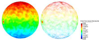
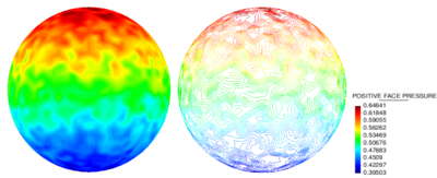
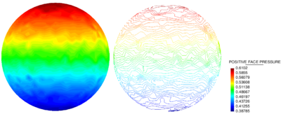
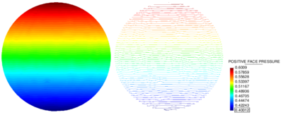
m (Cinmemj moved page Draft Samper 908356597 to Baumgartner et al 2015a) |
|||
| (37 intermediate revisions by the same user not shown) | |||
| Line 821: | Line 821: | ||
{| class="floating_imageSCP" style="text-align: center; border: 1px solid #BBB; margin: 1em auto; width: 100%;max-width: 100%;" | {| class="floating_imageSCP" style="text-align: center; border: 1px solid #BBB; margin: 1em auto; width: 100%;max-width: 100%;" | ||
|- | |- | ||
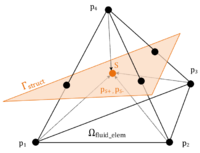
| − | |[[Image:draft_Samper_908356597-monograph-D01_ShapeFunctionConcept.png| | + | |[[Image:draft_Samper_908356597-monograph-D01_ShapeFunctionConcept.png|200px|'''Virtual subdivision of split element''' ]] |
|- style="text-align: center; font-size: 75%;" | |- style="text-align: center; font-size: 75%;" | ||
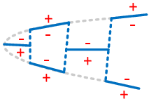
| colspan="1" | '''Figure 11:''' '''Virtual subdivision of split element''' | | colspan="1" | '''Figure 11:''' '''Virtual subdivision of split element''' | ||
| Line 861: | Line 861: | ||
{| class="floating_imageSCP" style="text-align: center; border: 1px solid #BBB; margin: 1em auto; width: 100%;max-width: 100%;" | {| class="floating_imageSCP" style="text-align: center; border: 1px solid #BBB; margin: 1em auto; width: 100%;max-width: 100%;" | ||
|- | |- | ||
| − | |[[Image:draft_Samper_908356597-monograph-D02_ShapeFunctionConcept_Duplication.png| | + | |[[Image:draft_Samper_908356597-monograph-D02_ShapeFunctionConcept_Duplication.png|200px|'''Separation of domain by duplication of nodes''' ]] |
|- style="text-align: center; font-size: 75%;" | |- style="text-align: center; font-size: 75%;" | ||
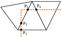
| colspan="1" | '''Figure 12:''' '''Separation of domain by duplication of nodes''' | | colspan="1" | '''Figure 12:''' '''Separation of domain by duplication of nodes''' | ||
| Line 869: | Line 869: | ||
{| class="floating_imageSCP" style="text-align: center; border: 1px solid #BBB; margin: 1em auto; width: 100%;max-width: 100%;" | {| class="floating_imageSCP" style="text-align: center; border: 1px solid #BBB; margin: 1em auto; width: 100%;max-width: 100%;" | ||
|- | |- | ||
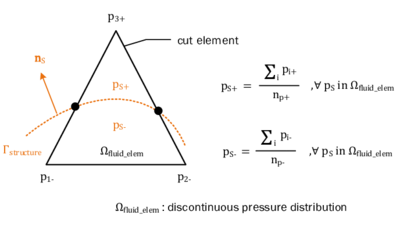
| − | |[[Image:draft_Samper_908356597-monograph-D03_ShapeFunctionConcept_Constraint.png| | + | |[[Image:draft_Samper_908356597-monograph-D03_ShapeFunctionConcept_Constraint.png|200px|'''Constraints on virtual nodes in a discontinuous element formulation''' ]] |
|- style="text-align: center; font-size: 75%;" | |- style="text-align: center; font-size: 75%;" | ||
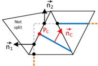
| colspan="1" | '''Figure 13:''' '''Constraints on virtual nodes in a discontinuous element formulation''' | | colspan="1" | '''Figure 13:''' '''Constraints on virtual nodes in a discontinuous element formulation''' | ||
| Line 934: | Line 934: | ||
{| class="floating_imageSCP" style="text-align: center; border: 1px solid #BBB; margin: 1em auto; width: 100%;max-width: 100%;" | {| class="floating_imageSCP" style="text-align: center; border: 1px solid #BBB; margin: 1em auto; width: 100%;max-width: 100%;" | ||
|- | |- | ||
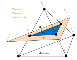
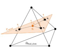
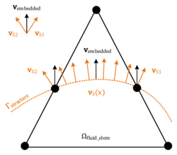
| − | |[[Image:draft_Samper_908356597-monograph-D06_EM_SlipCondition.png| | + | |[[Image:draft_Samper_908356597-monograph-D06_EM_SlipCondition.png|300px|'''Assumption of embedded velocity''' - Orange depicts the structure that is intersecting the fluid element and leading to the embedded boundary Γ in blue. Note that the embedded velocity is a function of the nodal velocities of the structure. ]] |
|- style="text-align: center; font-size: 75%;" | |- style="text-align: center; font-size: 75%;" | ||
| colspan="1" | '''Figure 16:''' '''Assumption of embedded velocity''' - Orange depicts the structure that is intersecting the fluid element and leading to the embedded boundary <math>\Gamma </math> in blue. Note that the embedded velocity is a function of the nodal velocities of the structure. | | colspan="1" | '''Figure 16:''' '''Assumption of embedded velocity''' - Orange depicts the structure that is intersecting the fluid element and leading to the embedded boundary <math>\Gamma </math> in blue. Note that the embedded velocity is a function of the nodal velocities of the structure. | ||
| Line 1,532: | Line 1,532: | ||
{| class="floating_imageSCP" style="text-align: center; border: 1px solid #BBB; margin: 1em auto; width: 100%;max-width: 100%;" | {| class="floating_imageSCP" style="text-align: center; border: 1px solid #BBB; margin: 1em auto; width: 100%;max-width: 100%;" | ||
|- | |- | ||
| − | |[[Image:draft_Samper_908356597-monograph-J01_FSI_coupling_interface.png| | + | |[[Image:draft_Samper_908356597-monograph-J01_FSI_coupling_interface.png|250px|'''FSI coupling interface''' - The fluid domain Ω<sub>F</sub> with the boundary Γ<sub>F</sub> and the structure domain Ω<sub>S</sub> with the boundary Γ<sub>S</sub> share the FSI interface Γ<sub>FSI</sub>.]] |
|- style="text-align: center; font-size: 75%;" | |- style="text-align: center; font-size: 75%;" | ||
| colspan="1" | '''Figure 18:''' '''FSI coupling interface''' - The fluid domain <math>\Omega _F</math> with the boundary <math>\Gamma _F</math> and the structure domain <math>\Omega _S</math> with the boundary <math>\Gamma _S</math> share the FSI interface <math>\Gamma _{FSI}</math>. | | colspan="1" | '''Figure 18:''' '''FSI coupling interface''' - The fluid domain <math>\Omega _F</math> with the boundary <math>\Gamma _F</math> and the structure domain <math>\Omega _S</math> with the boundary <math>\Gamma _S</math> share the FSI interface <math>\Gamma _{FSI}</math>. | ||
| Line 2,330: | Line 2,330: | ||
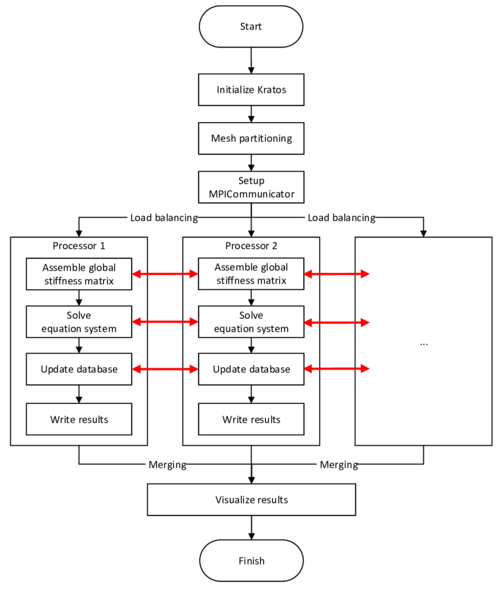
* ''Parallelization of FEM'': The idea of the spatial discretization of a fluid or a structure into small elements allows to decompose the domain into pieces which are assigned to multiple processors. Due to the fact that the element-wise contributions are separately assembled into the global stiffness matrix, the finite element computations can be executed on each processor separately. | * ''Parallelization of FEM'': The idea of the spatial discretization of a fluid or a structure into small elements allows to decompose the domain into pieces which are assigned to multiple processors. Due to the fact that the element-wise contributions are separately assembled into the global stiffness matrix, the finite element computations can be executed on each processor separately. | ||
* ''Making use of the powerful Spanish Supercomputing Network (Red Española de Supercomputación)'' | * ''Making use of the powerful Spanish Supercomputing Network (Red Española de Supercomputación)'' | ||
| + | <br /> | ||
Distributing the tremendous computational effort for a complex FSI simulation to multiple processors such that the computational efficiency improves, however, also brings some tricky challenges. The following list shows just the most significant challenges which we will face within this monograph: | Distributing the tremendous computational effort for a complex FSI simulation to multiple processors such that the computational efficiency improves, however, also brings some tricky challenges. The following list shows just the most significant challenges which we will face within this monograph: | ||
| Line 2,361: | Line 2,362: | ||
{| class="floating_imageSCP" style="text-align: center; border: 1px solid #BBB; margin: 1em auto; width: 100%;max-width: 100%;" | {| class="floating_imageSCP" style="text-align: center; border: 1px solid #BBB; margin: 1em auto; width: 100%;max-width: 100%;" | ||
|- | |- | ||
| − | |[[Image:draft_Samper_908356597-monograph-J01_SharedMemory.png| | + | |[[Image:draft_Samper_908356597-monograph-J01_SharedMemory.png|300px|'''Architecture of shared memory machines''' - All processors share the same memory.]] |
|- style="text-align: center; font-size: 75%;" | |- style="text-align: center; font-size: 75%;" | ||
| colspan="1" | '''Figure 26:''' '''Architecture of shared memory machines''' - All processors share the same memory. | | colspan="1" | '''Figure 26:''' '''Architecture of shared memory machines''' - All processors share the same memory. | ||
| Line 3,724: | Line 3,725: | ||
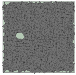
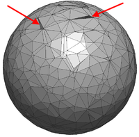
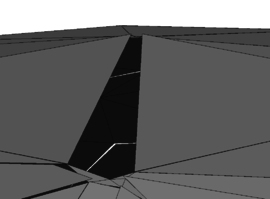
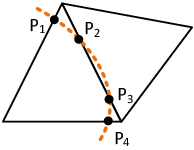
However, another obvious deficit is dominating in figure [[#img-68|68a]]. In the mesh interior there is a clear void without any triangles. Therefore it can not be the influence of the edge-near problem zone. Instead the reason turned out to be that some nodes of the fluid mesh coincide with the structure plane. This leads to an intersection pattern with one, two or even three intersection nodes directly located on a tetrahedron node as shown before in figures [[#img-55|55a]] and [[#img-55|55b]]. A simplified 2D visualization of this situation is shown in figure [[#img-69|69]]. | However, another obvious deficit is dominating in figure [[#img-68|68a]]. In the mesh interior there is a clear void without any triangles. Therefore it can not be the influence of the edge-near problem zone. Instead the reason turned out to be that some nodes of the fluid mesh coincide with the structure plane. This leads to an intersection pattern with one, two or even three intersection nodes directly located on a tetrahedron node as shown before in figures [[#img-55|55a]] and [[#img-55|55b]]. A simplified 2D visualization of this situation is shown in figure [[#img-69|69]]. | ||
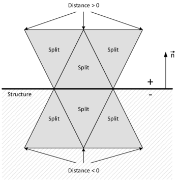
| − | Basically, all the visualized fluid elements are marked as split and the elemental distance vector contains one or two zero distance values. The problem with zero distances is that emanating from these structure-coinciding nodes no intersection point can be interpolated along the edges to that node as this requires a negative and a positive signed distance value. This implies that within the tetrahedron no triangle can be generated as no intersection point can be computed. Related to figure | + | Basically, all the visualized fluid elements are marked as split and the elemental distance vector contains one or two zero distance values. The problem with zero distances is that emanating from these structure-coinciding nodes no intersection point can be interpolated along the edges to that node as this requires a negative and a positive signed distance value. This implies that within the tetrahedron no triangle can be generated as no intersection point can be computed. Related to figure [[#img-68|68a]] there is one node which is coinciding with the structure plane. All tetrahedron which share this node will be neglected in the visualization function and therefore a hole is arising. A remedy for this is presented in the following section. |
====7.1.1.8 Strategy to eliminate zero-distance values==== | ====7.1.1.8 Strategy to eliminate zero-distance values==== | ||
| Line 3,753: | Line 3,754: | ||
{| class="floating_imageSCP" style="text-align: center; border: 1px solid #BBB; margin: 1em auto; width: 100%;max-width: 100%;" | {| class="floating_imageSCP" style="text-align: center; border: 1px solid #BBB; margin: 1em auto; width: 100%;max-width: 100%;" | ||
|- | |- | ||
| − | |[[Image:draft_Samper_908356597-monograph-J22_PlaneNoZeroDistances.png| | + | |[[Image:draft_Samper_908356597-monograph-J22_PlaneNoZeroDistances.png|300px|'''Representation of the plane after eliminating zero-distances''' - Compared to figure [[#img-69|69]] the hole does not appear any more.]] |
|- style="text-align: center; font-size: 75%;" | |- style="text-align: center; font-size: 75%;" | ||
| colspan="1" | '''Figure 71:''' '''Representation of the plane after eliminating zero-distances''' - Compared to figure [[#img-69|69]] the hole does not appear any more. | | colspan="1" | '''Figure 71:''' '''Representation of the plane after eliminating zero-distances''' - Compared to figure [[#img-69|69]] the hole does not appear any more. | ||
|} | |} | ||
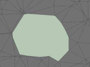
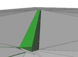
| − | The region around the node with a zero-distance is now completely closed as all the tetrahedra are able to represent the intersection pattern. The difference can be better shown in a direct comparison of this region - once without the local structure movement (figure | + | The region around the node with a zero-distance is now completely closed as all the tetrahedra are able to represent the intersection pattern. The difference can be better shown in a direct comparison of this region - once without the local structure movement (figure [[#img-72|72b]]) and with the zero distance correction (figure [[#img-72|72b]]). The right figure shows clearly that there was one node with a zero distance which is now forming numerous triangles to close the hole. |
This method conveys more advantages which go far beyond this demonstrated purpose. In the embedded method the nodes with zero-distance can be physically seen as part of the fluid <u>and</u> structure at the same time. There is no clear distinction between the properties which should be assigned to this node. How to treat these nodes in the formulation of the embedded approach? The set of modified shape functions of the split fluid elements - as explained in chapter [[#2.2.4.2 Element technology|2.2.4.2]] - is based on a clear distinction of each node to either fluid or structure, which is provided in any situation by the just discussed local interface-movement approach. | This method conveys more advantages which go far beyond this demonstrated purpose. In the embedded method the nodes with zero-distance can be physically seen as part of the fluid <u>and</u> structure at the same time. There is no clear distinction between the properties which should be assigned to this node. How to treat these nodes in the formulation of the embedded approach? The set of modified shape functions of the split fluid elements - as explained in chapter [[#2.2.4.2 Element technology|2.2.4.2]] - is based on a clear distinction of each node to either fluid or structure, which is provided in any situation by the just discussed local interface-movement approach. | ||
| − | |||
<div id='img-72'></div> | <div id='img-72'></div> | ||
{| class="floating_imageSCP" style="text-align: center; border: 1px solid #BBB; margin: 1em auto; width: 100%;max-width: 100%;" | {| class="floating_imageSCP" style="text-align: center; border: 1px solid #BBB; margin: 1em auto; width: 100%;max-width: 100%;" | ||
| Line 3,768: | Line 3,768: | ||
|[[Image:draft_Samper_908356597-monograph-J23_PlaneZeroZoom.png|288px|]] | |[[Image:draft_Samper_908356597-monograph-J23_PlaneZeroZoom.png|288px|]] | ||
|[[Image:draft_Samper_908356597-monograph-J24_PlaneNoZeroZoom.png|288px|'''Closer view to the region around a node with zero-distance - a comparison''' - The left figure is the result of the distance function which does not handle zero distance values - leading to a hole. The right figure solves this problem by a zero-distance correction.]] | |[[Image:draft_Samper_908356597-monograph-J24_PlaneNoZeroZoom.png|288px|'''Closer view to the region around a node with zero-distance - a comparison''' - The left figure is the result of the distance function which does not handle zero distance values - leading to a hole. The right figure solves this problem by a zero-distance correction.]] | ||
| + | |- style="text-align: center; font-size: 75%;" | ||
| + | | colspan="1" | (a) No zero-distance correction | ||
| + | | colspan="1" | (b) With zero-distance correction | ||
|- style="text-align: center; font-size: 75%;" | |- style="text-align: center; font-size: 75%;" | ||
| colspan="2" | '''Figure 72:''' '''Closer view to the region around a node with zero-distance - a comparison''' - The left figure is the result of the distance function which does not handle zero distance values - leading to a hole. The right figure solves this problem by a zero-distance correction. | | colspan="2" | '''Figure 72:''' '''Closer view to the region around a node with zero-distance - a comparison''' - The left figure is the result of the distance function which does not handle zero distance values - leading to a hole. The right figure solves this problem by a zero-distance correction. | ||
| Line 4,003: | Line 4,006: | ||
|- | |- | ||
| style="text-align: center;" | <math>\frac{\partial L}{\partial \boldsymbol{n}} = 2 \boldsymbol{A} \boldsymbol{n} + 2 \lambda \boldsymbol{n} = 0 </math> | | style="text-align: center;" | <math>\frac{\partial L}{\partial \boldsymbol{n}} = 2 \boldsymbol{A} \boldsymbol{n} + 2 \lambda \boldsymbol{n} = 0 </math> | ||
| + | |} | ||
| style="width: 5px;text-align: right;white-space: nowrap;" | (7.21) | | style="width: 5px;text-align: right;white-space: nowrap;" | (7.21) | ||
| + | |} | ||
| + | |||
| + | {| class="formulaSCP" style="width: 100%; text-align: left;" | ||
| + | |- | ||
| + | | | ||
| + | {| style="text-align: left; margin:auto;width: 100%;" | ||
|- | |- | ||
| style="text-align: center;" | <math> \frac{\partial L}{\partial \lambda } = \boldsymbol{n}^T \boldsymbol{n} - 1 = 0 </math> | | style="text-align: center;" | <math> \frac{\partial L}{\partial \lambda } = \boldsymbol{n}^T \boldsymbol{n} - 1 = 0 </math> | ||
| − | |||
|} | |} | ||
| + | | style="width: 5px;text-align: right;white-space: nowrap;" | (7.22) | ||
|} | |} | ||
| Line 4,456: | Line 4,466: | ||
<math display="inline">P_{C} \gets </math> mean(<math display="inline">nodes\_container</math>) | <math display="inline">P_{C} \gets </math> mean(<math display="inline">nodes\_container</math>) | ||
| + | |||
<math display="inline">\boldsymbol{n}_{C} \gets </math> mean(<math display="inline">normals\_container</math>) | <math display="inline">\boldsymbol{n}_{C} \gets </math> mean(<math display="inline">normals\_container</math>) | ||
| Line 4,470: | Line 4,481: | ||
|- | |- | ||
|[[Image:draft_Samper_908356597-monograph-J21_WingAfter_Solution2_Side.png|300px|]] | |[[Image:draft_Samper_908356597-monograph-J21_WingAfter_Solution2_Side.png|300px|]] | ||
| − | |||
|- style="text-align: center; font-size: 75%;" | |- style="text-align: center; font-size: 75%;" | ||
| colspan="1" | (a) Side view | | colspan="1" | (a) Side view | ||
| + | |- | ||
| + | |[[Image:draft_Samper_908356597-monograph-J22_WingAfter_Solution2_Front.png|300px|'''Wing model tested with the proposed approach''' - The applied approach is illustrated in figure [[#img-104|104]].]] | ||
| + | |- style="text-align: center; font-size: 75%;" | ||
| colspan="1" | (b) Front view | | colspan="1" | (b) Front view | ||
|- style="text-align: center; font-size: 75%;" | |- style="text-align: center; font-size: 75%;" | ||
| − | |||
| colspan="2" | '''Figure 105:''' '''Wing model tested with the proposed approach''' - The applied approach is illustrated in figure [[#img-104|104]]. | | colspan="2" | '''Figure 105:''' '''Wing model tested with the proposed approach''' - The applied approach is illustrated in figure [[#img-104|104]]. | ||
|} | |} | ||
| Line 4,858: | Line 4,870: | ||
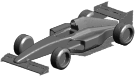
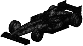
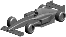
{| class="floating_imageSCP" style="text-align: center; border: 1px solid #BBB; margin: 1em auto; width: 100%;max-width: 100%;" | {| class="floating_imageSCP" style="text-align: center; border: 1px solid #BBB; margin: 1em auto; width: 100%;max-width: 100%;" | ||
|- | |- | ||
| − | |[[Image:draft_Samper_908356597-monograph-J01_FerrariStructureMesh.png| | + | |[[Image:draft_Samper_908356597-monograph-J01_FerrariStructureMesh.png|300px|'''Structure mesh of Formula 1 car''' - The surface model is meshed with 2.8e5 triangle elements.]] |
|- style="text-align: center; font-size: 75%;" | |- style="text-align: center; font-size: 75%;" | ||
| colspan="1" | '''Figure 126:''' '''Structure mesh of Formula 1 car''' - The surface model is meshed with <math>2.8e5</math> triangle elements. | | colspan="1" | '''Figure 126:''' '''Structure mesh of Formula 1 car''' - The surface model is meshed with <math>2.8e5</math> triangle elements. | ||
| Line 5,037: | Line 5,049: | ||
# Refinement strategy 1: 1 step | # Refinement strategy 1: 1 step | ||
| − | Applying this strategy to the fine-meshed structure (<math>2.5e5</math> elements) yields the approximation shown in figure [[#img-136|136]]. Already without any refinement, the shape of the tubes can be roughly captured (figure [[#img-136|136a]]). The curvature and the sharp edges at the base, however, can not be represented accurately. After the first three refinement steps (figure [[#img-136|136c]]) the hangar approximation converges very well to the original model. Solely the surface of the tube exhibits some edged indentations which can be smoothed by applying strategy 1 again as shown in figure | + | Applying this strategy to the fine-meshed structure (<math>2.5e5</math> elements) yields the approximation shown in figure [[#img-136|136]]. Already without any refinement, the shape of the tubes can be roughly captured (figure [[#img-136|136a]]). The curvature and the sharp edges at the base, however, can not be represented accurately. After the first three refinement steps (figure [[#img-136|136c]]) the hangar approximation converges very well to the original model. Solely the surface of the tube exhibits some edged indentations which can be smoothed by applying strategy 1 again as shown in figure [[#img-136|136c]]. The precise representation of the sharp edges at the base is shown in figure [[#img-136|136d]]. |
<div id='img-136'></div> | <div id='img-136'></div> | ||
{| class="floating_imageSCP" style="text-align: center; border: 1px solid #BBB; margin: 1em auto; width: 100%;max-width: 100%;" | {| class="floating_imageSCP" style="text-align: center; border: 1px solid #BBB; margin: 1em auto; width: 100%;max-width: 100%;" | ||
| Line 6,282: | Line 6,294: | ||
|[[Image:draft_Samper_908356597-monograph-D33_Averaging_results_01.png|400px|]] | |[[Image:draft_Samper_908356597-monograph-D33_Averaging_results_01.png|400px|]] | ||
|- style="text-align: center; font-size: 75%;" | |- style="text-align: center; font-size: 75%;" | ||
| − | | colspan="1" | (a) elemets/circumference = 14 | + | | colspan="1" | (a) ''elemets/circumference'' = 14 |
|- | |- | ||
|[[Image:draft_Samper_908356597-monograph-D33_Averaging_results_02.png|400px|'''Results of pressure mapping by arithmetic averaging''' - The results are shown for two different levels of refinement of the fluid domain.]] | |[[Image:draft_Samper_908356597-monograph-D33_Averaging_results_02.png|400px|'''Results of pressure mapping by arithmetic averaging''' - The results are shown for two different levels of refinement of the fluid domain.]] | ||
|- style="text-align: center; font-size: 75%;" | |- style="text-align: center; font-size: 75%;" | ||
| − | | colspan="1" | (b) elemets/circumference = 94 | + | | colspan="1" | (b) ''elemets/circumference'' = 94 |
|- style="text-align: center; font-size: 75%;" | |- style="text-align: center; font-size: 75%;" | ||
| colspan="1" | '''Figure 189:''' '''Results of pressure mapping by arithmetic averaging''' - The results are shown for two different levels of refinement of the fluid domain. | | colspan="1" | '''Figure 189:''' '''Results of pressure mapping by arithmetic averaging''' - The results are shown for two different levels of refinement of the fluid domain. | ||
| Line 6,467: | Line 6,479: | ||
{| style="text-align: left; margin:auto;width: 100%;" | {| style="text-align: left; margin:auto;width: 100%;" | ||
|- | |- | ||
| − | | style="text-align: center;" | <math>\begin{array}{ccc}\\ \left[~\boldsymbol{x}_I(\boldsymbol{\eta }_I) ~\right]^T \\ \\ \end{array} = \boldsymbol{N}_{local} (\boldsymbol{\eta }_I) | + | | style="text-align: center;" | <math>\begin{array}{ccc}\\ \left[~\boldsymbol{x}_I(\boldsymbol{\eta }_I) ~\right]^T \\ \\ \end{array} = \boldsymbol{N}_{local} (\boldsymbol{\eta }_I) \cdot \left[ \begin{array}{ccc}&&\\ \boldsymbol{x}_1 & \boldsymbol{x}_2 & \boldsymbol{x}_3\\ & &\end{array} \right] \begin{array}{ccc}\\ \end{array} </math> |
| − | + | ||
| − | + | ||
|} | |} | ||
| style="width: 5px;text-align: right;white-space: nowrap;" | (8.25) | | style="width: 5px;text-align: right;white-space: nowrap;" | (8.25) | ||
| Line 6,726: | Line 6,736: | ||
{| class="floating_imageSCP" style="text-align: center; border: 1px solid #BBB; margin: 1em auto; width: 100%;max-width: 100%;" | {| class="floating_imageSCP" style="text-align: center; border: 1px solid #BBB; margin: 1em auto; width: 100%;max-width: 100%;" | ||
|- | |- | ||
| − | |[[Image:draft_Samper_908356597-monograph-D51_Setup_InflatableMembrane.png| | + | |[[Image:draft_Samper_908356597-monograph-D51_Setup_InflatableMembrane.png|500px|'''Setup of an inflatable membrane in a CFD context''' ]] |
|- style="text-align: center; font-size: 75%;" | |- style="text-align: center; font-size: 75%;" | ||
| colspan="1" | '''Figure 208:''' '''Setup of an inflatable membrane in a CFD context''' | | colspan="1" | '''Figure 208:''' '''Setup of an inflatable membrane in a CFD context''' | ||
|} | |} | ||
| − | + | <span id='table-12'></span> | |
| − | {| class="floating_tableSCP wikitable" style="text-align: | + | {| class="floating_tableSCP wikitable" style="text-align: center; margin: 1em auto;min-width:50%;" |
| − | |+ style="font-size: 75%;" | | + | |+ style="font-size: 75%;" |Table. 12 '''Material parameters''' |
| − | |- | + | |- style="border-top: 2px solid;border-bottom: 2px solid;" |
| <math display="inline">\rho _{Membrane}</math> | | <math display="inline">\rho _{Membrane}</math> | ||
| <math>E_{Membrane}</math> | | <math>E_{Membrane}</math> | ||
| Line 6,740: | Line 6,750: | ||
| <math>\rho _{Fluid}</math> | | <math>\rho _{Fluid}</math> | ||
| <math>\mu _{Fluid}</math> | | <math>\mu _{Fluid}</math> | ||
| − | |- | + | |- style="border-top: 2px solid;border-bottom: 2px solid;" |
| <math display="inline">1.1 \cdot 10^3</math> | | <math display="inline">1.1 \cdot 10^3</math> | ||
| <math>1.0 \cdot 10^5</math> | | <math>1.0 \cdot 10^5</math> | ||
| Line 6,760: | Line 6,770: | ||
The corresponding boundary conditions can be found in figure [[#img-209|209]]. | The corresponding boundary conditions can be found in figure [[#img-209|209]]. | ||
| − | |||
<div id='img-209'></div> | <div id='img-209'></div> | ||
{| class="floating_imageSCP" style="text-align: center; border: 1px solid #BBB; margin: 1em auto; width: 100%;max-width: 100%;" | {| class="floating_imageSCP" style="text-align: center; border: 1px solid #BBB; margin: 1em auto; width: 100%;max-width: 100%;" | ||
| Line 6,766: | Line 6,775: | ||
|[[Image:draft_Samper_908356597-monograph-D52_inflatableMembrane_p_BC.png|294px|]] | |[[Image:draft_Samper_908356597-monograph-D52_inflatableMembrane_p_BC.png|294px|]] | ||
|[[Image:draft_Samper_908356597-monograph-D52_inflatableMembrane_v_BC.png|294px|'''Prescribed quantities in the simplified hangar scenario''']] | |[[Image:draft_Samper_908356597-monograph-D52_inflatableMembrane_v_BC.png|294px|'''Prescribed quantities in the simplified hangar scenario''']] | ||
| + | |- style="text-align: center; font-size: 75%;" | ||
| + | | colspan="1" | (a) Prescribed inflatation of the membrane | ||
| + | | colspan="1" | (b) Prescribed flow | ||
|- style="text-align: center; font-size: 75%;" | |- style="text-align: center; font-size: 75%;" | ||
| colspan="2" | '''Figure 209:''' '''Prescribed quantities in the simplified hangar scenario''' | | colspan="2" | '''Figure 209:''' '''Prescribed quantities in the simplified hangar scenario''' | ||
| Line 6,774: | Line 6,786: | ||
Before discussing the simulation results, however, it is worthwhile to have a look at the different finite element models that needed to be prepared for the intended comparison. The single models are illustrated in figure [[#img-210|210]]. Without having computed anything the first and one of the most convincing advantages becomes already obvious. That is the advantage of a significantly eased pre-processing in the embedded approach. Whereas for the ALE method a detailed and explicit modeling of the interface is necessary, the embedded approach only requires a simple background fluid mesh which may be obtained very quickly by automated meshing routines. Depending on the intended level of accuracy, this may indeed contain areas with different refinement, but creating the latter is still significantly faster than an explicit modeling of the actual interface. In this context it is interesting, that the structure model may be the same in both cases, which means that for the embedded approach given models from earlier simulations may be recycled and do not have to be modeled again. This in fact is an additional advantage regarding the necessary pre-processing which might facilitate a possible change of the solution procedure from the ALE approach to the embedded approach. | Before discussing the simulation results, however, it is worthwhile to have a look at the different finite element models that needed to be prepared for the intended comparison. The single models are illustrated in figure [[#img-210|210]]. Without having computed anything the first and one of the most convincing advantages becomes already obvious. That is the advantage of a significantly eased pre-processing in the embedded approach. Whereas for the ALE method a detailed and explicit modeling of the interface is necessary, the embedded approach only requires a simple background fluid mesh which may be obtained very quickly by automated meshing routines. Depending on the intended level of accuracy, this may indeed contain areas with different refinement, but creating the latter is still significantly faster than an explicit modeling of the actual interface. In this context it is interesting, that the structure model may be the same in both cases, which means that for the embedded approach given models from earlier simulations may be recycled and do not have to be modeled again. This in fact is an additional advantage regarding the necessary pre-processing which might facilitate a possible change of the solution procedure from the ALE approach to the embedded approach. | ||
| − | After having modeled the example for both solution approaches it is each simulated for maximum <math display="inline">10s</math>. The simulation is, however, expected to fail earlier due to reasons that we will see later. In the ALE-case we furthermore want to use two different mesh-updating strategies, i.e. the Laplacian mesh-updating with adaptive conductivity and the structure-like alternative. This shall allow us to evaluate the possible improvements in more detail. For the corresponding quantitative evaluation, we are looking at the two distinct nodes that were already given in figure [[#img-208|208]]. To be more precise, we are evaluating the flow-induced displacement at node | + | After having modeled the example for both solution approaches it is each simulated for maximum <math display="inline">10s</math>. The simulation is, however, expected to fail earlier due to reasons that we will see later. In the ALE-case we furthermore want to use two different mesh-updating strategies, i.e. the Laplacian mesh-updating with adaptive conductivity and the structure-like alternative. This shall allow us to evaluate the possible improvements in more detail. For the corresponding quantitative evaluation, we are looking at the two distinct nodes that were already given in figure [[#img-208|208]]. To be more precise, we are evaluating the flow-induced displacement at node "<math display="inline">D</math>" and the resulting pressure evolution at node "<math display="inline">P</math>". Let us first have a look on the displacements of node <math display="inline">D</math> in <math display="inline">X</math> and <math display="inline">Y</math>. The corresponding results are given in figure [[#img-211|211]] and [[#img-212|212]], respectively. |
| − | |||
<div id='img-210'></div> | <div id='img-210'></div> | ||
{| class="floating_imageSCP" style="text-align: center; border: 1px solid #BBB; margin: 1em auto; width: 100%;max-width: 100%;" | {| class="floating_imageSCP" style="text-align: center; border: 1px solid #BBB; margin: 1em auto; width: 100%;max-width: 100%;" | ||
|- | |- | ||
| − | |[[Image:draft_Samper_908356597-monograph-D53_Model_Fluid_EM.png| | + | |[[Image:draft_Samper_908356597-monograph-D53_Model_Fluid_EM.png|200px|]] |
| − | |[[Image:draft_Samper_908356597-monograph-D53_Model_Fluid_ALE.png| | + | |[[Image:draft_Samper_908356597-monograph-D53_Model_Fluid_ALE.png|200px|]] |
| + | |- style="text-align: center; font-size: 75%;" | ||
| + | | colspan="1" | (a) Fluid model in an embedded approach | ||
| + | | colspan="1" | (b) Fluid model in an ALE approach | ||
|- | |- | ||
| colspan="2"|[[Image:draft_Samper_908356597-monograph-D53_Model_Structure.png|294px|'''Possible pre-processing in the embedded and body-fitted approach''']] | | colspan="2"|[[Image:draft_Samper_908356597-monograph-D53_Model_Structure.png|294px|'''Possible pre-processing in the embedded and body-fitted approach''']] | ||
| + | |- style="text-align: center; font-size: 75%;" | ||
| + | | colspan="2" | (c) Common structure model | ||
|- style="text-align: center; font-size: 75%;" | |- style="text-align: center; font-size: 75%;" | ||
| colspan="2" | '''Figure 210:''' '''Possible pre-processing in the embedded and body-fitted approach''' | | colspan="2" | '''Figure 210:''' '''Possible pre-processing in the embedded and body-fitted approach''' | ||
| Line 6,791: | Line 6,807: | ||
{| class="floating_imageSCP" style="text-align: center; border: 1px solid #BBB; margin: 1em auto; width: 100%;max-width: 100%;" | {| class="floating_imageSCP" style="text-align: center; border: 1px solid #BBB; margin: 1em auto; width: 100%;max-width: 100%;" | ||
|- | |- | ||
| − | |[[Image:draft_Samper_908356597-monograph-D54_inflatableMembrane_XDisp.png| | + | |[[Image:draft_Samper_908356597-monograph-D54_inflatableMembrane_XDisp.png|400px|'''Flow induced X-movement of node D from figure [[#img-208|208]]''']] |
|- style="text-align: center; font-size: 75%;" | |- style="text-align: center; font-size: 75%;" | ||
| colspan="1" | '''Figure 211:''' '''Flow induced <math>X</math>-movement of node <math>D</math> from figure [[#img-208|208]]''' | | colspan="1" | '''Figure 211:''' '''Flow induced <math>X</math>-movement of node <math>D</math> from figure [[#img-208|208]]''' | ||
|} | |} | ||
| − | |||
<div id='img-212'></div> | <div id='img-212'></div> | ||
{| class="floating_imageSCP" style="text-align: center; border: 1px solid #BBB; margin: 1em auto; width: 100%;max-width: 100%;" | {| class="floating_imageSCP" style="text-align: center; border: 1px solid #BBB; margin: 1em auto; width: 100%;max-width: 100%;" | ||
|- | |- | ||
| − | |[[Image:draft_Samper_908356597-monograph-D54_inflatableMembrane_YDisp.png| | + | |[[Image:draft_Samper_908356597-monograph-D54_inflatableMembrane_YDisp.png|400px|]] |
| − | + | ||
|- style="text-align: center; font-size: 75%;" | |- style="text-align: center; font-size: 75%;" | ||
| − | | colspan=" | + | | colspan="1" | (a) Over entire simulation |
| + | |- | ||
| + | |[[Image:draft_Samper_908356597-monograph-D54_inflatableMembrane_YDisp_cutout.png|400px|'''Flow induced Y-movement of node D from figure [[#img-208|208]]''']] | ||
| + | |- style="text-align: center; font-size: 75%;" | ||
| + | | colspan="1" | (b) Close-up at failure of the ALE solution | ||
| + | |- style="text-align: center; font-size: 75%;" | ||
| + | | colspan="1" | '''Figure 212:''' '''Flow induced <math>Y</math>-movement of node <math>D</math> from figure [[#img-208|208]]''' | ||
|} | |} | ||
First striking fact seen in both figures is, that with the embedded approach we are able to resolve a significantly wider range of movements compared to the ALE case. In particular it can be seen, that while the ALE-approach already fails<span id="fnc-44"></span>[[#fn-44|<sup>1</sup>]] during the inflation, the embedded approach allows to continue the simulation up to the point of the flow-induced deflection of the inflated membrane. So it is not critically influenced from the complex dynamics of the structure. Figure [[#img-213|213]] and [[#img-214|214]] illustrate the results from the embedded solution for two different instances in time according to the two different load stages. | First striking fact seen in both figures is, that with the embedded approach we are able to resolve a significantly wider range of movements compared to the ALE case. In particular it can be seen, that while the ALE-approach already fails<span id="fnc-44"></span>[[#fn-44|<sup>1</sup>]] during the inflation, the embedded approach allows to continue the simulation up to the point of the flow-induced deflection of the inflated membrane. So it is not critically influenced from the complex dynamics of the structure. Figure [[#img-213|213]] and [[#img-214|214]] illustrate the results from the embedded solution for two different instances in time according to the two different load stages. | ||
| − | |||
<div id='img-213'></div> | <div id='img-213'></div> | ||
{| class="floating_imageSCP" style="text-align: center; border: 1px solid #BBB; margin: 1em auto; width: 100%;max-width: 100%;" | {| class="floating_imageSCP" style="text-align: center; border: 1px solid #BBB; margin: 1em auto; width: 100%;max-width: 100%;" | ||
|- | |- | ||
| − | |[[Image:draft_Samper_908356597-monograph-D55_Velocity_NoWind.png| | + | |[[Image:draft_Samper_908356597-monograph-D55_Velocity_NoWind.png|350px|]] |
| − | |[[Image:draft_Samper_908356597-monograph-D55_Pressure_NoWind.png| | + | |- style="text-align: center; font-size: 75%;" |
| − | + | | colspan="1" | (a) Driving velocity field(Fluid model with embedded structure) | |
| − | ]] | + | |- |
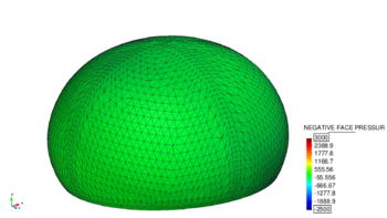
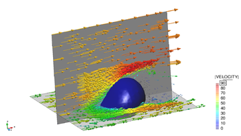
| + | |[[Image:draft_Samper_908356597-monograph-D55_Pressure_NoWind.png|350px|'''Inflation of the membrane inside the environmental fluid''' - The figures show a snap-shot at t = 7.5s during the inflation phase]] | ||
| + | |- style="text-align: center; font-size: 75%;" | ||
| + | | colspan="1" | (b) Induced surface pressure (Structure model with mapped pressure) | ||
|- style="text-align: center; font-size: 75%;" | |- style="text-align: center; font-size: 75%;" | ||
| − | | colspan=" | + | | colspan="1" | '''Figure 213:''' '''Inflation of the membrane inside the environmental fluid''' - The figures show a snap-shot at t = 7.5s during the inflation phase |
|} | |} | ||
| − | |||
<div id='img-214'></div> | <div id='img-214'></div> | ||
{| class="floating_imageSCP" style="text-align: center; border: 1px solid #BBB; margin: 1em auto; width: 100%;max-width: 100%;" | {| class="floating_imageSCP" style="text-align: center; border: 1px solid #BBB; margin: 1em auto; width: 100%;max-width: 100%;" | ||
|- | |- | ||
| − | |[[Image:draft_Samper_908356597-monograph-D56_Velocity_InWind.png| | + | |[[Image:draft_Samper_908356597-monograph-D56_Velocity_InWind.png|350px|]] |
| − | |[[Image:draft_Samper_908356597-monograph-D56_Pressure_InWind.png| | + | |- style="text-align: center; font-size: 75%;" |
| + | | colspan="1" | (a) Driving velocity field(Fluid model with embedded structure) | ||
| + | |- | ||
| + | |[[Image:draft_Samper_908356597-monograph-D56_Pressure_InWind.png|350px|'''Flow induced movement of the coupled membrane''' - The figures show a snap-shot of the resulting fluid-structure interaction during the active fluid flow at t = 8.75s]] | ||
| + | |- style="text-align: center; font-size: 75%;" | ||
| + | | colspan="1" | (b) Induced surface pressure (Structure model with mapped pressure) | ||
|- style="text-align: center; font-size: 75%;" | |- style="text-align: center; font-size: 75%;" | ||
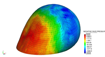
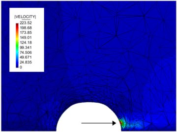
| colspan="2" | '''Figure 214:''' '''Flow induced movement of the coupled membrane''' - The figures show a snap-shot of the resulting fluid-structure interaction during the active fluid flow at <math>t = 8.75s</math> | | colspan="2" | '''Figure 214:''' '''Flow induced movement of the coupled membrane''' - The figures show a snap-shot of the resulting fluid-structure interaction during the active fluid flow at <math>t = 8.75s</math> | ||
| Line 6,834: | Line 6,860: | ||
Second striking fact when looking at the displacement diagrams is, that changing the mesh-updating strategy in the ALE case only yields comparatively small improvements in terms of possible movements that can be simulated. This means here, that with none of the given mesh-updating strategies we were able to simulate the entire inflation together with the later deflection phase. Only the change to the embedded solution procedure really allows to overcome the respective limitations. Putting this in a more general context, one may realize that with an ALE-solution procedure there will be ''always'' a limit beyond which a proper mesh-update is not possible anymore<span id="fnc-45"></span>[[#fn-45|<sup>2</sup>]]. So having an FSI problem where such a limit is reached, it may be very attractive to choose an embedded solution approach instead of trying various different sophisticated and possibly costly mesh-updating strategies which only allow for a certain shift of the limits instead of really overcoming them. | Second striking fact when looking at the displacement diagrams is, that changing the mesh-updating strategy in the ALE case only yields comparatively small improvements in terms of possible movements that can be simulated. This means here, that with none of the given mesh-updating strategies we were able to simulate the entire inflation together with the later deflection phase. Only the change to the embedded solution procedure really allows to overcome the respective limitations. Putting this in a more general context, one may realize that with an ALE-solution procedure there will be ''always'' a limit beyond which a proper mesh-update is not possible anymore<span id="fnc-45"></span>[[#fn-45|<sup>2</sup>]]. So having an FSI problem where such a limit is reached, it may be very attractive to choose an embedded solution approach instead of trying various different sophisticated and possibly costly mesh-updating strategies which only allow for a certain shift of the limits instead of really overcoming them. | ||
| − | Third, when looking in particular at the <math display="inline">Y</math>-displacement in figure [[#img- | + | Third, when looking in particular at the <math display="inline">Y</math>-displacement in figure [[#img-212|212b]] it can be observed, that there in fact is a quantitative difference in the results. Assuming that the ALE-approach generally is more accurate than the embedded one, this difference may be regarded as true accuracy loss. How this accuracy loss actually influences the principle behavior of the structure and to what extend the system's dynamic is affected by that are still two open questions which could not be answered in the scope of this work. It is nevertheless interesting to note that in this example the simulated principal movement of the membrane up to the point of failure is qualitatively the same with either approach. |
Apart from the movement, also the actual failure situation is interesting. Looking at the results, it can be observed, that the embedded and the ALE approach fail due to two ''different'' reasons. While the ALE approach does not come across an inappropriate mesh-update, which is a numerical problem arising from the explicit modeling of the coupling interface, the embedded approach fails because either of the single partitions, i.e. the fluid model or the structure model, fails, which is not a problem of the coupling but rather more a question of the quality of the single field models. In this example for instance, the embedded FSI approach failed because the structure simulation failed, which in turn is the consequence of invalid element formations that occur due to the fact that we are despite this large movements neglecting physical effects like self contact etc.. Figure [[#img-215|215]] shows the corresponding failure situation of the structure model in the embedded case. The failing mesh-update in the ALE case is illustrated in figure [[#img-216|216]]. | Apart from the movement, also the actual failure situation is interesting. Looking at the results, it can be observed, that the embedded and the ALE approach fail due to two ''different'' reasons. While the ALE approach does not come across an inappropriate mesh-update, which is a numerical problem arising from the explicit modeling of the coupling interface, the embedded approach fails because either of the single partitions, i.e. the fluid model or the structure model, fails, which is not a problem of the coupling but rather more a question of the quality of the single field models. In this example for instance, the embedded FSI approach failed because the structure simulation failed, which in turn is the consequence of invalid element formations that occur due to the fact that we are despite this large movements neglecting physical effects like self contact etc.. Figure [[#img-215|215]] shows the corresponding failure situation of the structure model in the embedded case. The failing mesh-update in the ALE case is illustrated in figure [[#img-216|216]]. | ||
| Line 6,841: | Line 6,867: | ||
{| class="floating_imageSCP" style="text-align: center; border: 1px solid #BBB; margin: 1em auto; width: 100%;max-width: 100%;" | {| class="floating_imageSCP" style="text-align: center; border: 1px solid #BBB; margin: 1em auto; width: 100%;max-width: 100%;" | ||
|- | |- | ||
| − | |[[Image:draft_Samper_908356597-monograph-D57_Membrane_Failure_01.png| | + | |[[Image:draft_Samper_908356597-monograph-D57_Membrane_Failure_01.png|400px|'''Failure of structure model in the embedded case''' - The picture shows the actual structure model with mapped surface pressure at t = 9.3s. Note the interpenetrating and overlapping elements.]] |
|- style="text-align: center; font-size: 75%;" | |- style="text-align: center; font-size: 75%;" | ||
| colspan="1" | '''Figure 215:''' '''Failure of structure model in the embedded case''' - The picture shows the actual structure model with mapped surface pressure at <math>t = 9.3s</math>. Note the interpenetrating and overlapping elements. | | colspan="1" | '''Figure 215:''' '''Failure of structure model in the embedded case''' - The picture shows the actual structure model with mapped surface pressure at <math>t = 9.3s</math>. Note the interpenetrating and overlapping elements. | ||
| Line 6,861: | Line 6,887: | ||
{| class="floating_imageSCP" style="text-align: center; border: 1px solid #BBB; margin: 1em auto; width: 100%;max-width: 100%;" | {| class="floating_imageSCP" style="text-align: center; border: 1px solid #BBB; margin: 1em auto; width: 100%;max-width: 100%;" | ||
|- | |- | ||
| − | |[[Image:draft_Samper_908356597-monograph-D58_inflatableMembrane_p01.png| | + | |[[Image:draft_Samper_908356597-monograph-D58_inflatableMembrane_p01.png|400px|'''Pressure evolution at node P from figure [[#img-208|208]]''']] |
|- style="text-align: center; font-size: 75%;" | |- style="text-align: center; font-size: 75%;" | ||
| colspan="1" | '''Figure 217:''' '''Pressure evolution at node <math>P</math> from figure [[#img-208|208]]''' | | colspan="1" | '''Figure 217:''' '''Pressure evolution at node <math>P</math> from figure [[#img-208|208]]''' | ||
| Line 6,869: | Line 6,895: | ||
{| class="floating_imageSCP" style="text-align: center; border: 1px solid #BBB; margin: 1em auto; width: 100%;max-width: 100%;" | {| class="floating_imageSCP" style="text-align: center; border: 1px solid #BBB; margin: 1em auto; width: 100%;max-width: 100%;" | ||
|- | |- | ||
| − | |[[Image:draft_Samper_908356597-monograph-D58_inflatableMembrane_p02.png| | + | |[[Image:draft_Samper_908356597-monograph-D58_inflatableMembrane_p02.png|400px|'''Close-up of the pressure evolution at node P from figure [[#img-208|208]]''']] |
|- style="text-align: center; font-size: 75%;" | |- style="text-align: center; font-size: 75%;" | ||
| colspan="1" | '''Figure 218:''' '''Close-up of the pressure evolution at node <math>P</math> from figure [[#img-208|208]]''' | | colspan="1" | '''Figure 218:''' '''Close-up of the pressure evolution at node <math>P</math> from figure [[#img-208|208]]''' | ||
| Line 6,876: | Line 6,902: | ||
Second interesting fact is revealed when looking a little closer at the pressure gradient in the beginning of the simulation as depicted in figure [[#img-218|218]]. Looking at this close-up we first note that the results in both the different solution approaches actually cannot be significantly compared since the FSI-simulation crashes, too, quickly in case of the ALE approach. A quantitative confrontation of the different solution approaches hence is not possible. Nevertheless what is interesting is the fact that in the embedded approach the flow initialization phase, where we observe a periodic converging pressure gradient, seems to be considerably quicker and also in terms of its magnitude significantly less distinct. It is obvious that this is an effect of the weak imposition of the boundary conditions at the coupling interface in the embedded approach which naturally tends to damp oscillations. This damping may also be regarded as some kind of additional robustness advantage of the embedded approach in contrast to the ALE procedure. It is, however, clear, that this numerical damping at the same time affects the accuracy of the solution. | Second interesting fact is revealed when looking a little closer at the pressure gradient in the beginning of the simulation as depicted in figure [[#img-218|218]]. Looking at this close-up we first note that the results in both the different solution approaches actually cannot be significantly compared since the FSI-simulation crashes, too, quickly in case of the ALE approach. A quantitative confrontation of the different solution approaches hence is not possible. Nevertheless what is interesting is the fact that in the embedded approach the flow initialization phase, where we observe a periodic converging pressure gradient, seems to be considerably quicker and also in terms of its magnitude significantly less distinct. It is obvious that this is an effect of the weak imposition of the boundary conditions at the coupling interface in the embedded approach which naturally tends to damp oscillations. This damping may also be regarded as some kind of additional robustness advantage of the embedded approach in contrast to the ALE procedure. It is, however, clear, that this numerical damping at the same time affects the accuracy of the solution. | ||
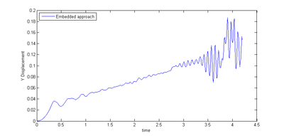
| − | Having now seen a few of the major advantages of the embedded approach, an important negative effect, that was encountered during the above analysis, shall be mentioned. To this end we have a look at the vertical displacement of node <math display="inline">D</math> when the above membrane is inflated comparatively slowly. The corresponding displacement curve is depicted in figure [[#img-219|219]]. Due to the very slow inflation of the membrane we in the beginning do not get this oscillating movement as we saw it in figure | + | Having now seen a few of the major advantages of the embedded approach, an important negative effect, that was encountered during the above analysis, shall be mentioned. To this end we have a look at the vertical displacement of node <math display="inline">D</math> when the above membrane is inflated comparatively slowly. The corresponding displacement curve is depicted in figure [[#img-219|219]]. Due to the very slow inflation of the membrane we in the beginning do not get this oscillating movement as we saw it in figure [[#img-211|211a]] but rather more a steadily growing membrane after a short transient phase. Actually this is what we physically expected from a slowly inflated membrane. Nevertheless, when continuing the simulation, at around <math display="inline">t = 2.75s</math>, suddenly a highly dynamic behavior forms out, which continues to grow more and more as the structure keeps inflating. |
The reason for this unexpected dynamic behavior was found to be the mapping problem described in chapter [[#8.3.2 Persisting problems with pressure mapping|8.3.2]]. Due to the curved shape of the membrane locally bad intersection patterns formed out. At the corresponding spots then the actual pressure conditions could not be resolved properly which eventually influenced the system dynamics critically. This observation emphasizes the demand for a powerful ''and'' robust mapping technique since possible limitations might not necessarily lead to a crashing simulation, where we are technically able to observe a problem free of doubt. Instead they can just initiate or change the dynamic behavior which is much more subtle and hence significantly more difficult to encounter. | The reason for this unexpected dynamic behavior was found to be the mapping problem described in chapter [[#8.3.2 Persisting problems with pressure mapping|8.3.2]]. Due to the curved shape of the membrane locally bad intersection patterns formed out. At the corresponding spots then the actual pressure conditions could not be resolved properly which eventually influenced the system dynamics critically. This observation emphasizes the demand for a powerful ''and'' robust mapping technique since possible limitations might not necessarily lead to a crashing simulation, where we are technically able to observe a problem free of doubt. Instead they can just initiate or change the dynamic behavior which is much more subtle and hence significantly more difficult to encounter. | ||
| Line 6,883: | Line 6,909: | ||
{| class="floating_imageSCP" style="text-align: center; border: 1px solid #BBB; margin: 1em auto; width: 100%;max-width: 100%;" | {| class="floating_imageSCP" style="text-align: center; border: 1px solid #BBB; margin: 1em auto; width: 100%;max-width: 100%;" | ||
|- | |- | ||
| − | |[[Image:draft_Samper_908356597-monograph-D59_inflatableMembrane_problem.png| | + | |[[Image:draft_Samper_908356597-monograph-D59_inflatableMembrane_problem.png|400px|'''Artificial dynamic behavior during inflation due to mapping problems.''' - The figure shows the vertical displacement of the membrane during a comparatively slow inflation. Note that the simulation did not numerically fail but was finished intentionally.]] |
|- style="text-align: center; font-size: 75%;" | |- style="text-align: center; font-size: 75%;" | ||
| colspan="1" | '''Figure 219:''' '''Artificial dynamic behavior during inflation due to mapping problems.''' - The figure shows the vertical displacement of the membrane during a comparatively slow inflation. Note that the simulation did not numerically fail but was finished intentionally. | | colspan="1" | '''Figure 219:''' '''Artificial dynamic behavior during inflation due to mapping problems.''' - The figure shows the vertical displacement of the membrane during a comparatively slow inflation. Note that the simulation did not numerically fail but was finished intentionally. | ||
| Line 6,907: | Line 6,933: | ||
{| class="floating_imageSCP" style="text-align: center; border: 1px solid #BBB; margin: 1em auto; width: 100%;max-width: 100%;" | {| class="floating_imageSCP" style="text-align: center; border: 1px solid #BBB; margin: 1em auto; width: 100%;max-width: 100%;" | ||
|- | |- | ||
| − | |[[Image:draft_Samper_908356597-monograph-D61_bucklingMembraneSetup.png| | + | |[[Image:draft_Samper_908356597-monograph-D61_bucklingMembraneSetup.png|350px|'''3D setup of the flow-induced buckling of a membrane''']] |
|- style="text-align: center; font-size: 75%;" | |- style="text-align: center; font-size: 75%;" | ||
| colspan="1" | '''Figure 220:''' '''3D setup of the flow-induced buckling of a membrane''' | | colspan="1" | '''Figure 220:''' '''3D setup of the flow-induced buckling of a membrane''' | ||
| Line 6,915: | Line 6,941: | ||
{| class="floating_imageSCP" style="text-align: center; border: 1px solid #BBB; margin: 1em auto; width: 100%;max-width: 100%;" | {| class="floating_imageSCP" style="text-align: center; border: 1px solid #BBB; margin: 1em auto; width: 100%;max-width: 100%;" | ||
|- | |- | ||
| − | |[[Image:draft_Samper_908356597-monograph-D62_BucklingMembrane_Velocity.png| | + | |[[Image:draft_Samper_908356597-monograph-D62_BucklingMembrane_Velocity.png|350px|'''3D model of the flow-induced buckling of a membrane''']] |
|- style="text-align: center; font-size: 75%;" | |- style="text-align: center; font-size: 75%;" | ||
| colspan="1" | '''Figure 221:''' '''3D model of the flow-induced buckling of a membrane''' | | colspan="1" | '''Figure 221:''' '''3D model of the flow-induced buckling of a membrane''' | ||
| Line 6,925: | Line 6,951: | ||
{| class="floating_imageSCP" style="text-align: center; border: 1px solid #BBB; margin: 1em auto; width: 100%;max-width: 100%;" | {| class="floating_imageSCP" style="text-align: center; border: 1px solid #BBB; margin: 1em auto; width: 100%;max-width: 100%;" | ||
|- | |- | ||
| − | |[[Image:draft_Samper_908356597-monograph-D63_BuckMembrane_P.png| | + | |[[Image:draft_Samper_908356597-monograph-D63_BuckMembrane_P.png|300px|'''Gradient of stagnation pressure at point C from figure [[#img-220|220]]''']] |
|- style="text-align: center; font-size: 75%;" | |- style="text-align: center; font-size: 75%;" | ||
| colspan="1" | '''Figure 222:''' '''Gradient of stagnation pressure at point <math>C</math> from figure [[#img-220|220]]''' | | colspan="1" | '''Figure 222:''' '''Gradient of stagnation pressure at point <math>C</math> from figure [[#img-220|220]]''' | ||
| Line 6,933: | Line 6,959: | ||
{| class="floating_imageSCP" style="text-align: center; border: 1px solid #BBB; margin: 1em auto; width: 100%;max-width: 100%;" | {| class="floating_imageSCP" style="text-align: center; border: 1px solid #BBB; margin: 1em auto; width: 100%;max-width: 100%;" | ||
|- | |- | ||
| − | |[[Image:draft_Samper_908356597-monograph-D63_BuckMembrane_D.png| | + | |[[Image:draft_Samper_908356597-monograph-D63_BuckMembrane_D.png|300px|'''Gradient of absolute displacement at point C from figure [[#img-220|220]]''']] |
|- style="text-align: center; font-size: 75%;" | |- style="text-align: center; font-size: 75%;" | ||
| colspan="1" | '''Figure 223:''' '''Gradient of absolute displacement at point <math>C</math> from figure [[#img-220|220]]''' | | colspan="1" | '''Figure 223:''' '''Gradient of absolute displacement at point <math>C</math> from figure [[#img-220|220]]''' | ||
| Line 6,945: | Line 6,971: | ||
{| class="floating_imageSCP" style="text-align: center; border: 1px solid #BBB; margin: 1em auto; width: 100%;max-width: 100%;" | {| class="floating_imageSCP" style="text-align: center; border: 1px solid #BBB; margin: 1em auto; width: 100%;max-width: 100%;" | ||
|- | |- | ||
| − | |[[Image:draft_Samper_908356597-monograph-D64_BuckMembrane_Contours.png| | + | |[[Image:draft_Samper_908356597-monograph-D64_BuckMembrane_Contours.png|500px|'''Flow-induced buckling of a membrane''' - The left sequence plots the displacements as contours whereas the right sequence shows a lateral cut through the membrane at y = 0.05 for the different time instances.]] |
|- style="text-align: center; font-size: 75%;" | |- style="text-align: center; font-size: 75%;" | ||
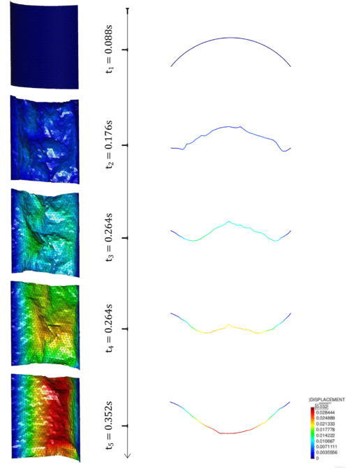
| colspan="1" | '''Figure 224:''' '''Flow-induced buckling of a membrane''' - The left sequence plots the displacements as contours whereas the right sequence shows a lateral cut through the membrane at <math>y = 0.05</math> for the different time instances. | | colspan="1" | '''Figure 224:''' '''Flow-induced buckling of a membrane''' - The left sequence plots the displacements as contours whereas the right sequence shows a lateral cut through the membrane at <math>y = 0.05</math> for the different time instances. | ||
| Line 6,952: | Line 6,978: | ||
Looking at the herein depicted deformation pattern, one can see that in fact the embedded approach handles the massively occurring wrinkles without any problems. So despite the complex mesh configuration of the structure, the FSI simulation remains stable without any additional loss of accuracy. Obviously, when using a body-fitted approach, this would not be the case, since a mesh-updating procedure would most probably fail at a certain instance in particular at highly transient spots with local peaks and valleys such as they appear in the middle of the membrane. One typical remedy in the latter case certainly might be a complete re-meshing. But since the wrinkles are occurring during the entire simulation a re-meshing would have to be performed in each step causing an explosion of the computational costs. Moreover, even with a re-meshing there is no guarantee that all the elements in the fluid are properly distributed. So in fact we observe a superior robustness of the embedded approach when comparing it to any body-fitted method, such as the ALE approach. | Looking at the herein depicted deformation pattern, one can see that in fact the embedded approach handles the massively occurring wrinkles without any problems. So despite the complex mesh configuration of the structure, the FSI simulation remains stable without any additional loss of accuracy. Obviously, when using a body-fitted approach, this would not be the case, since a mesh-updating procedure would most probably fail at a certain instance in particular at highly transient spots with local peaks and valleys such as they appear in the middle of the membrane. One typical remedy in the latter case certainly might be a complete re-meshing. But since the wrinkles are occurring during the entire simulation a re-meshing would have to be performed in each step causing an explosion of the computational costs. Moreover, even with a re-meshing there is no guarantee that all the elements in the fluid are properly distributed. So in fact we observe a superior robustness of the embedded approach when comparing it to any body-fitted method, such as the ALE approach. | ||
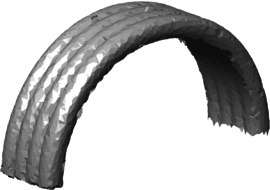
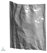
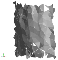
| − | At this point it is worthwhile to recap also from the other chapters, that the herein presented embedded method poses a particularly robust method for fluid-structure interaction analysis because of three facts: Firstly there is no technical link between the different discretizations involved, which is why any mesh-update generally becomes obsolete. Nevertheless, there exists of course a coupling. Here, however, the velocities are applied in a weak sense which yields a second robustness benefit. Third and last reason is based on the fact that an embedded approach introduces implicitly a certain length-scale below which no structural detail can be resolved. The length-scale is thereby defined by the background fluid mesh. So every detail of an embedded structure which is smaller than the corresponding size of the background fluid element will not be captured. This implicitly filters problematic local effects such as wrinkles. For an impression see figure [[#img-225|225]]. It is the last reason that mainly affects the accuracy of the solution, which is why for this simulation again the earlier presented refinement strategy was applied. So in the present simulation the structure is seen by the embedded solver as shown in figure [[#img- | + | At this point it is worthwhile to recap also from the other chapters, that the herein presented embedded method poses a particularly robust method for fluid-structure interaction analysis because of three facts: Firstly there is no technical link between the different discretizations involved, which is why any mesh-update generally becomes obsolete. Nevertheless, there exists of course a coupling. Here, however, the velocities are applied in a weak sense which yields a second robustness benefit. Third and last reason is based on the fact that an embedded approach introduces implicitly a certain length-scale below which no structural detail can be resolved. The length-scale is thereby defined by the background fluid mesh. So every detail of an embedded structure which is smaller than the corresponding size of the background fluid element will not be captured. This implicitly filters problematic local effects such as wrinkles. For an impression see figure [[#img-225|225]]. It is the last reason that mainly affects the accuracy of the solution, which is why for this simulation again the earlier presented refinement strategy was applied. So in the present simulation the structure is seen by the embedded solver as shown in figure [[#img-225|225c]]. |
| − | |||
<div id='img-225'></div> | <div id='img-225'></div> | ||
{| class="floating_imageSCP" style="text-align: center; border: 1px solid #BBB; margin: 1em auto; width: 100%;max-width: 100%;" | {| class="floating_imageSCP" style="text-align: center; border: 1px solid #BBB; margin: 1em auto; width: 100%;max-width: 100%;" | ||
|- | |- | ||
| − | |[[Image:draft_Samper_908356597-monograph-D64_SkinMesh_01.png| | + | | colspan="2" |[[Image:draft_Samper_908356597-monograph-D64_SkinMesh_01.png|200px|]] |
| − | | | + | |- style="text-align: center; font-size: 75%;" |
| + | | colspan="2" | (a) Structure mesh | ||
|- | |- | ||
| − | | | + | |[[Image:draft_Samper_908356597-monograph-D64_SkinMesh_03.png|200px|]] |
| + | |[[Image:draft_Samper_908356597-monograph-D64_SkinMesh_02.png|200px|'''Structure mesh and its embedded representation at t = 0.15s''']] | ||
| + | |- style="text-align: center; font-size: 75%;" | ||
| + | | colspan="1" | (b) Coarse representation within the fluid (35000 fluid elements) | ||
| + | | colspan="1" | (c) Refined representation within the fluid (250000 fluid elemenets) | ||
|- style="text-align: center; font-size: 75%;" | |- style="text-align: center; font-size: 75%;" | ||
| colspan="2" | '''Figure 225:''' '''Structure mesh and its embedded representation at <math>t = 0.15s</math>''' | | colspan="2" | '''Figure 225:''' '''Structure mesh and its embedded representation at <math>t = 0.15s</math>''' | ||
Latest revision as of 13:22, 6 June 2019
Abstract
Designing large ultra-lightweight structures within a fluid flow, such as inflatable hangars in an atmospheric environment, requires an analysis of the naturally occurring fluid-structure interaction (FSI). To this end multidisciplinary simulation techniques may be used. The latter, though, have to be capable of dealing with complex shapes and large deformations as well as challenging phenomena like wrinkling or folding of the structure. To overcome such problems the method of embedded domains may be used. In this work we discuss a new solution procedure for FSI analyses based on the method of embedded domains. In doing so, we are in particular answering the questions: How to track the interface in the embedded approach, how does the subsequent solution procedure look like and how does both compare to the well-known Arbitrary Lagrangian-Eulerian (ALE) approach? In this context a level set technique as well as different mapping and mesh-updating strategies are developed and evaluated. Furthermore the solution procedure of a completely embedded FSI analysis is established and tested using different small- and large-scale examples. All results are finally compared to results from an ALE approach. It is shown that the embedded approach offers a powerful and robust alternative in terms of the FSI analysis of ultra-lightweight structures with complex shapes and large deformations. With regard to the solution accuracy, however, clear restrictions are elaborated.
Acknowledgements
This monograph was written at the International Center for Numerical Methods in Engineering (CIMNE, Barcelona) based on a joint research project with the Technical University Munich (TUM) during the period from May to December 2013. During that time, we gained vast experience in numerical methods, software development and their practical application to solve complex engineering problems within a dynamic and innovative research team. The project, however, would not have been possible without the tremendous support of Riccardo Rossi (CIMNE) and Roland Wüchner (TUM). Both of them contributed decisively to the success of this work and are responsible for a challenging but exciting topic branching into the world of FSI simulations.
Roland Wüchner dedicated himself to the subject with a lot of interest that he showed during the numerous intercontinental sessions where he often sacrificed his valuable evenings for an in-depth discussion. He reserved many hours to shape the subject in detail in order to guarantee a benefit for all the contributors. Moreover, he constantly motivated us by guiding and refining all our ideas. The same is true for Riccardo Rossi. He offered a fantastic technical and personal support in all questions that arose. Many of the here presented ideas were driven by his support or on his initiative. We thank you both a lot!
Furthermore, we want to thank Pooyan Dadvand and Jordi Cotela who provided us with the implementation of many functionalities in Kratos. For any kind of problem with Kratos they patiently did intensive investigations until the problem was solved. In general, we acknowledge the support of every single person of the Kratos and the GiD team.
Finally, all the authors wish to thank the ERC for the support under the projects uLites FP7-SME-2012 GA n.314891 and NUMEXAS FP7-ICT-611636.
1 Introduction
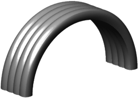
Objects of interest within the scope of this work are inflatable mobile light-weight hangars for the application in aerospace industry (See figure 1). Purpose of such a hangar is to cover aircrafts ranging from smaller propeller machines up to large scale passenger aircraft both from civil and military services. The advantage of such a structure is obvious: It offers the possibility to flexibly and quickly build up and position a hangar without occupying expensive and rare space permanently. This allows a fast reaction to current needs such as the protection of single aircraft from weather influences or the setup of a provisional operating base while being protected from external surveillance.
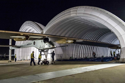 ] ]
|
| Figure 1: Example of an inflatable hangar - Adopted from [1] |
In order to ensure functionality and safety, prior tests regarding the structure's behavior within the environmental fluid, i.e. an air flow, are essential. Here the investigation of the respective fluid-structure-interaction is of particular importance due to the lightweight concept being strongly affected by e.g. wind loads. Physical tests in this regards are, however, very costly since the lightweight concept does typically not allow for any scaling of the model to smaller sizes. This means, that a physical test always requires a very cost-intensive full-scale model. That is the reason why people are particularly interested in the powerful as well as resource- and cost-efficient virtual design analysis, which in this case means a computational analysis of the fluid-structure interaction (FSI).
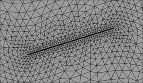
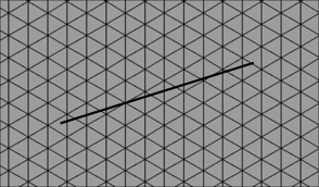
Requirement for the corresponding coupled simulation, though, is the ability to deal with large deformations, wrinkling or folding, respectively. To this end a simulation technology based on the method of embedded domains1 is developed at the International Center of Numerical Methods in Engineering (CIMNE). The method of embedded domains is an alternative methodology for the computation of partial differential equations and as such offers the interesting advantage of efficiently dealing with complex boundaries and large deformations where a body-fitted technique like the Arbitrary Lagrangian-Eulerian method (ALE) for examples uses an often expensive moving domain discretization (“Moving Mesh”). Particularly in the scope of fluid-structure interaction analysis, the embedded methods allows to separately handle the different physical entities without having to account for a specific interface model. Instead different overlapping discretizations ("embedded meshes") are used. See figure 2 for an illustration of the different approaches.
In this context, the goal of the present monograph is 1) the further development of the at CIMNE developed method of embedded domains such that it may be used for large-scale CFD and FSI problems and 2) the evaluation of the method compared to the well-known ALE approach. In doing so the tasks were split into two key topics: first the interface tracking in the embedded case and second the setup and comparison of the FSI solution procedure in both cases. For the interface tracking in the embedded method, level set techniques were to be implemented and verified. In terms of the solution procedures the goal was to develop and implement different mesh-updating strategies in the ALE-case as well as mapping techniques for the embedded method. Hence different test scenarios of coupled fluid-structure problems were to be developed, set up and simulated in order to finally compare the methods. For the sake of software modularity focus was here set on partitioned solution techniques. Furthermore in order to keep the computational costs of the coupled analyses as low as possible, parallelization techniques ought to be applied throughout the entire implementation phase.
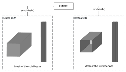
The software environment was generally given by the CIMNE in-house multiphysics finite element solver “Kratos”. For the partitioned analysis furthermore the simulation environment EMPIRE (“Enhanced Multi Physics Interface Research Engine”, Technical University Munich) was to be used. So an additional specification arising from this context required the set up of an interface between both software frameworks in order to be able to use the full functionality of EMPIRE together with all features in Kratos. Perspectively the goal is to use Kratos via EMPIRE together with the at the Technical University Munich (TUM) developed structural solver “Carat++” in a common partitioned FSI-environment. This shall allow to combine and consolidate capabilities of either software package and hence the knowledge of either of the related research groups.
Based on all the aforementioned goals, the present monograph is organized as follows: In the first section (chapter 2 to 4) the theoretical background regarding the analysis of coupled fluid-structure problems is given. Here it starts with a discussion of the single field problems which subsequently is extended and merged to the fundamentals of coupled fluid-structure analyses. In both cases the above stated and newly in Kratos implemented method of embedded domains is introduced in detail. Part of the theoretical framework is also a discussion of how in both approaches the computational efficiency may be improved. This includes the presentation of parallelization techniques as well as spatial search algorithms specifically applied in case of the embedded method.
In the second section then (chapter 5 to 6) the different applied software packages as well as the corresponding software interface are described. Here the contents are presented in a very application oriented way in order to provide a documentation for future users.
In the third section (chapter 7) the first key topic of the present monograph is elaborated, i.e. the interface tracking in the scope of the embedded method. Here we answer the questions regarding how to track the interface with two overlapping meshes and how does this affect the corresponding solution quality. Therefore different geometry examples, from a generic structure to a large scale Formula One car, are investigated. Furthermore in this context, different fluid problems are simulated with the embedded method and subsequently evaluated.
Having discussed how to track the interface in the embedded case and knowing about the situation in a body-fitted approach, the fourth section (chapter 8) is dedicated to the second key topic of this monograph, i.e. the actual solution procedure with fluid-structure simulations using either of the aforementioned methods. Here the different developed process steps are elaborated and evaluated in detail giving finally a complete overview of the entire solution process in both cases. With all the implementations then at hand, two solution examples of fully coupled problems are presented which eventually allows for a comparison of the two different approaches.
Finally all the results are briefly summarized and contrasted to the above stated goals.
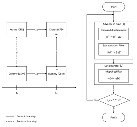
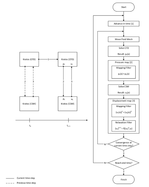
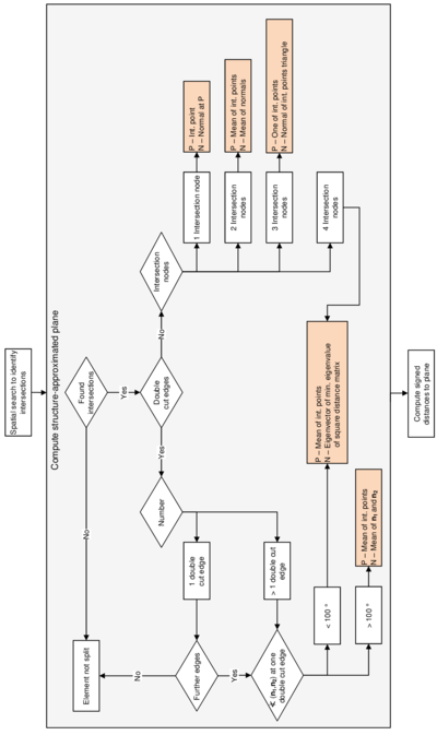
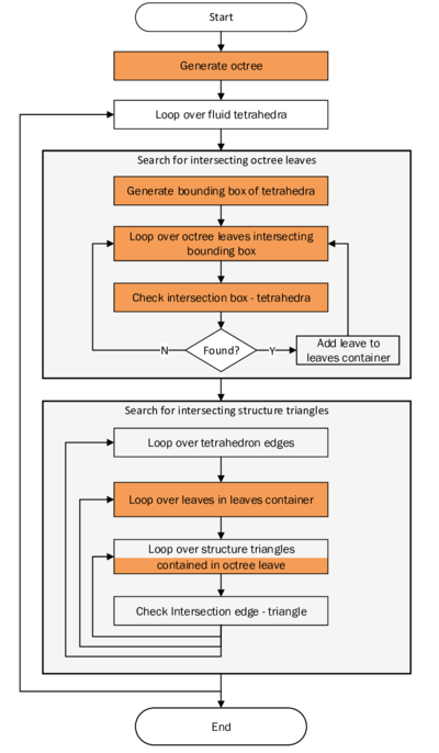
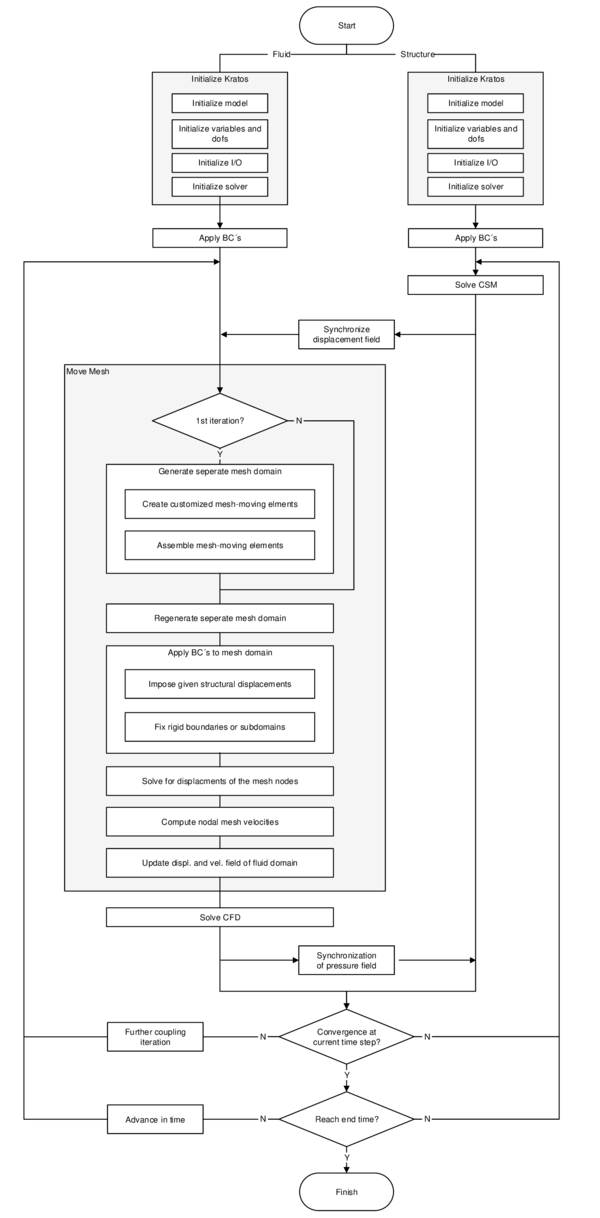
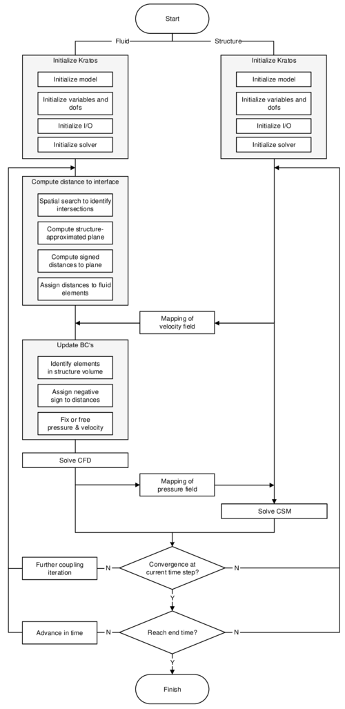
In order to facilitate the understanding of the later presented developments, the two process flows corresponding to the two different solution approaches as they were established in Kratos, shall be outlined here in advance (3, 4)2. For now, they shall just give an idea about the necessary steps to establish a coupled fluid-structure simulation using one of the above mentioned approaches. In the later course of this monograph then, whenever a feature is discussed or developed, its integration into the overall process is illustrated by means of these two charts. This allows to see importance and impact of single developments in a more general context.
|
| Figure 3: Partitioned FSI simulation using the ALE approach |
|
| Figure 4: Partitioned FSI simulation using the embedded approach |
(1) In literature also called “immersed” or “fix-grid” methods
(2) Note that both of the depicted processes show a partitioned analysis
2 Fluid and structure as uncoupled fields
In the following the mechanical fundamentals of fluids and structures shall be discussed together with their numerical treatment, i.e. their spatial discretization via FEM, their time discretization using different time integration schemes and their solution by some selected procedures. Both fluid and structure will be regarded as a continuum. Consequently their formulation will be similar and based on classical continuum mechanics. Given this assumption, the chapter will start with a brief introduction into the general description of motion according to basic continuum mechanics. Actual differences between structures and fluids from the point of view of their mechanical description will be elaborated in the later course of the chapter. Afterwards the method of embedded domains will be introduced into the context of classical fluid mechanics. Particularly the relevant element formulation will be of interest here. A discussion of how to impose corresponding boundary conditions will finally close the chapter.
2.1 Lagrangian and Eulerian description of motion
In continuum mechanics there are different ways to describe motion. We will focus in this context on the most established ones for each the structure and the fluid. For detailed information in this context, the reader is referred to the classical textbooks of Malvern [2] or Donea [3] and Cengel [4].
In the referential description the motion is described with respect to a reference configuration in which a particle of the continuum is located on the position at time . It is called Lagrangian description when the reference configuration coincides with the initial configuration at . In elasticity theory the initial configuration is typically chosen to be the unstressed state. Within the Lagrangian viewpoint, one keeps track of the motion of an individual material particle by recording the position of a particle at a time linking its material coordinates to the spatial coordinates via the function :
|
|
(2.1) |
Computationally this means that each individual node of a discretized domain is permanently attached to an associated material particle at any point of time as shown in figure 5. When the motion results in large deformations and therefore large distortions of the computational mesh, this method approaches a limit and might even fail due to excessively distorted finite elements which are linked to the material particles.
![Lagrangian viewpoint - The computational grid follows the material particles in the course of their motion (adapted from [3]).](/wd/images/thumb/7/71/Draft_Samper_908356597-monograph-J01_LagrangianConfiguration.png/400px-Draft_Samper_908356597-monograph-J01_LagrangianConfiguration.png)
|
| Figure 5: Lagrangian viewpoint - The computational grid follows the material particles in the course of their motion (adapted from [3]). |
On the contrary, the spatial description - also called the Eulerian description - avoids such difficulties by considering a control volume fixed in space. In that case the continuum is moving and deforming relatively to the discretized domain of the control volume. We do not keep track of the motion of an individual material particle, rather we observe how the flow field at the fixed computational mesh nodes is changing over time by introducing field variables within the control volume. For example, the spatial description of the velocity field can be defined as a field function of the spatial coordinates and the time instant :
|
|
(2.2) |
In this equation it becomes obvious that there is no link to the initial configuration or the material coordinates . Moreover, the velocity of the material at a given node of the computational grid is associated to the velocity of the material particle coinciding with the node. It is also possible to conclude from the flow field at given nodes to the total rate of change of the flow field when following a particle that moves through the fluid domain. This is done via the material derivative which basically links the Eulerian and the Lagrangian description. Applied to a pressure field, the relation is as follows:
|
|
(2.3) |
or correspondingly for the velocity field, it reads:
|
|
(2.4) |
The first part on the right hand side is called the local or unsteady term describing the local rate of change and the second part is the convective term constituting the rate of change of a particle when it moves to a region with different pressure or velocity.
Table 1 is supposed to contrast the most significant advantages and disadvantages of the two descriptions of motion. In order to combine the advantages of both Lagrangian and Eulerian description of motion the so-called Arbitrary Lagrangian-Eulerian method (ALE) has been developed. This method will be treated in chapter 3.2.2.
| Lagrangian description | Eulerian description |
| Allows to keep track of the history-dependent material behavior and to back-reference from the current configuration to the initial configuration of any material particle. | Does not permit to conclude from the current configuration to the initial configuration and the material coordinates . |
| The coincidence of material particles and the computational grid affects that the convective term drops out in the material derivative 2.4 leading to a simple time derivative. | The computational mesh is decoupled from the motion of material particles resulting in a convective term (see formula 2.4). The numerical handling of such a convective term leads to difficulties due to its nonsymmetric character. |
| Following the motion of the particles might lead to excessive distortions of the finite elements when no remeshing is applied what in turn can cause numerical problems during simulation. | Due to the fixed computational mesh there are no distortions of finite elements such that large motion and deformation in the continuum can be analyzed. |
| Is mostly used in structure mechanics, free surface flow and simulations incorporating moving interfaces between different materials (e.g. FSI). | Application especially in the field of fluid mechanics (e.g. simulation of vortices). Following free surfaces and interfaces between different materials comes along with larger numerical effort. |
2.2 Computational fluid mechanics
Within this chapter the fundamental formulation of the fluid mechanical problem, that is applied throughout this monograph, shall be introduced. Thereby we will first discuss the governing equations, their numerical discretization in space and time as well as an established solution procedure. Unless stated elsewhere, we will restrict ourselves to a Eulerian description of motion. Furthermore in this context we will focus on finite element techniques as well as the fractional step solution method, which both accounts for the later application in problems related to fluid-structure interaction. In all explanations we will closely follow the theoretical basics given in [3], the implementation and solver related details from chapter 3 in [6] and some specific research results in terms of the finite element method for fluid analysis elaborated in [7,8].
In the second part then a newly developed embedded approach shall be introduced, with which simulations, comprising highly deforming structures in a CFD context, shall be eased significantly. In here we will explain, based on the finite element method, both the new modeling technique and its corresponding immanent assumptions. It shall be of particular importance here that the latter assumptions are introduced critically and if necessary linked to corresponding investigations contained in the later course of the present monograph. All of the explanations will furthermore be kept general in that sense that it can be easily transferred from a shear CFD to a fully coupled FSI analysis.
2.2.1 Governing equations
The first step in describing the mechanics of a material, including fluids, is the assumption about the underlying material model. We will in the following rely on the continuum assumption which models the material as a continuous mass rather than for instance as discrete particles1. Based on this assumption any material is governed by the conservation of linear momentum:
|
|
(2.5) |
the conservation of mass:
|
|
(2.6) |
and the conservation of energy.
|
|
(2.7) |
where is the velocity vector, is the density, is the physical pressure, the body force vector, the sum of internal and kinetic energies, the heat flux vector, and and are the internal heat generation and internal heat dissipation function, respectively. The equations here are written in conservative form, which means they are arranged such, that they actually show that the overall change of a quantity is zero, i.e. the quantity is conserved. Note that the system is completely coupled, i.e. a solution of one equation is not possible without taking into account all the others.
Now we will introduce the following assumptions: 1) All state variables are continuous in space so their derivatives exist, 2) the fluid is considered to be incompressible, which yields
|
|
(2.8) |
and 3) the fluid is considered Newtonian, with constant viscosity, where
|
|
(2.9) |
Here, describes the Cauchy stress, the dynamic viscosity, the symmetric part of the velocity gradient and is the identity matrix. In fact the latter assumption about the material constitution represents the only major difference between the description of a fluid, as it is done here, and the description of a structure whose constitutive relation is typically given in the form . Note that the latter is based on the actual strains rather than the strain rates as they are implied in 2.9.
A consequence of these assumptions is, that the energy conservation is not anymore necessary to sufficiently describe the mechanical system. Thus for an incompressible flow, instead of four governing equations (conservation of momentum, mass and energy as well as the constitutive equation) we only have two simplified partial differential equations with the two independent state variables and 2. The remaining two equations with all the above assumptions included are known as the incompressible Navier-Stokes equations (NSE), which are typically given in the non-conservative form:
|
|
(2.10.a) |
|
|
(2.10.b) |
Here is the kinematic viscosity and the kinematic pressure. Note that the NSE describe a non-linear, coupled dynamic system.
Eventually we have the choice to either express w.r.t. a stationary coordinate system, where corresponds to the physical velocity at a given fixed point in space (Eulerian approach) or a moving coordinate system (Lagrangian approach), where is determined from the point of view of the moving fluid particle. These approaches can also be combined in a generalized formulation in order to be able to resolve the dynamics of the different domains in an FSI context, as we will see later.
To ensure that the system has a unique solution and to make the problem well posed, it is finally necessary to prescribe exactly one boundary condition at each the Neumann and the Dirichlet boundary. The NSE hence pose a classical boundary value problem where a strong imposition of the latter boundary conditions reads:
|
|
(2.11.a) |
|
|
(2.11.b) |
The assumption of initial conditions in the form
|
|
(2.12.a) |
|
|
(2.12.b) |
completes the problem formulation. Having now mathematically formalized the underlying physics. We have to discretize the NSE in order to solve it numerically.
(1) A famous particle-based model in computational fluid dynamics is e.g. the Lattice-Boltzmann-Method.
(2) Note that the velocity is a three-dimensional vector actually resulting in four independent state variables. The number of equations within the NSE increases accordingly.
2.2.2 Discretization
The NSE can be discretized in various ways both in time and space. All solutions throughout this monograph, though, were computed based on a finite element discretization in space and finite difference schemes in time which is why the latter techniques shall be introduced in the following. We will thereby follow an idea which in the literature is called the method of lines.
The method of lines is a usual practice in finite analysis of time-dependent problems. In here we are first discretizing with respect to the spatial variables from which we obtain a system of coupled first-order ordinary differential equations (with respect to time). The latter is called the semi-discrete system. Then to complete the discretization of the original PDE, we integrate the first-order differential system forward in time to trace the temporal evolution of the solution starting form the initial point .
2.2.2.1 Spatial discretization
Within this section it is assumed that the reader is familiar with the basic concepts of the finite element method using variational calculus.
Given the NSE, its weak form is obtained by multiplying 2.10.a and 2.10.b with the test functions and respectively. The corresponding weighted residual formulation reads:
|
|
(2.13.a) |
|
|
(2.13.b) |
By performing an integration by parts of the viscous term and the pressure gradient term in the momentum balance and each applying the divergence theorem the final weak form of the NSE is obtained as:
|
|
(2.14.a) |
|
|
(2.14.b) |
It can be seen from the equation, that by this approach we have naturally produced a Neumann boundary which is now given in a weak formulation as:
|
|
(2.15) |
where describes the boundary normal. In this weak formulation the Dirichlet boundary terms vanish since the test-functions and are by definition zero on the Dirichlet boundary. This implies that, given that is part of the solution of the NSE, the Dirichlet boundary conditions are automatically fulfilled. One important practical example of a Dirichlet boundary condition is the application of no-slip-conditions on walls.
At this point it shall be mentioned that for the imposition of slip boundary conditions by contrast, we may partially integrate 2.13.b such that we get:
|
|
(2.16) |
Then we split the boundary term in parts where we want to enforce slip-conditions and parts where we do not. This may read:
|
|
(2.17) |
By simply omitting the computation of the slip-boundary integral during the simulation, i.e.
|
|
(2.18) |
we imply that the velocities along this parts of the boundary are in a weak sense perpendicular to the local boundary normals . This basically reflects a tangent sliding of the fluid along the respective walls and hence an imposition of a slip boundary condition.
To finish the spatial discretization we introduce linear shape functions in order to approximate and as well as and . Here a Galerkin formulation is used where shape functions and test-functions are of the same kind. By assuming Einstein's summation convention, the approximation reads:
|
|
(2.19) |
|
|
(2.20) |
|
|
(2.21) |
|
|
(2.22) |
Plugging these interpolations into the weak form of the NSE given by equation 2.14.a and 2.14.b we obtain the following semi-discrete form of the incompressible NSE:
|
|
(2.23) |
where on elemental level
|
|
(2.24.a) |
|
|
(2.24.b) |
|
|
(2.24.c) |
|
|
(2.24.d) |
|
|
(2.24.e) |
|
|
(2.24.f) |
Note that the problem is still time dependent. That is, we still need to introduce a time discretization scheme in order to assemble the local contributions to a global system that can be solved. Note also that and here are the approximated quantities of the velocity and the pressure. Since this will be the case for the remainder of the monograph, we will refrain from an indexation for the sake of readability. For the actual computation in an FEM framework, numerical integration methods (such as Gauss-Integration) are necessary to compute the integrals in 2.24.
At the end of this section two basic problems shall be mentioned, that arise in this form of the discretization: The first problem occurs in cases where the convective term is dominant, for example in high-Reynolds or turbulent flows. In these cases the standard Galerkin approach gets unstable. Another numerical difficulty arises from the incompressibility constraint. In incompressible flows the pressure is acting as a Lagrange multiplier that enforces the velocity not to violate the mass conservation in a very strong form. The role of the pressure variable is thus to adjust itself instantaneously to the given velocity field such that the mass conservation holds.This leads to a coupling between the velocity and the pressure unknowns that causes the system in 2.23 to get ill-conditioned or even singular.
Both problems lead to the fact that in an FEM formulated flow problem, the compliance to certain numerical conditions or the application of stabilization techniques are inevitable.
2.2.2.2 Time discretization
Given the first order time dependent, semi-discrete NSE in 2.23, we may use a variety of different methods to integrate in time and hence compute the numerical solution of the NSE. Depending on the application we may therefore use either single step or multistep methods in an explicit or implicit formulation. Famous classes of integration schemes which are based on a single time step are: the list of Runge-Kutta methods or all customized integrators from the Newmark-family. A vast source of detailed information, in particular also in terms of accuracy order or stability, can be found in [9]. For a quick reference about the principal idea of the time integration chapter 3.4.1 in [3] is recommended.
By contrast, a famous class of integration schemes based on multi-step procedures is given by the different schemes of the Backward Differentiation Formula (BDF). In fact the BDF scheme of second order, i.e. BDF-2, is used by the fractional step solver, with which the solutions throughout this monograph were generated.
In the BDF-2 scheme, unlike in other multi-step integration variants, we, for a given function and time, approximate the time derivative of quantities rather than the quantities itself by incorporating information from previous, current and following time-steps. This typically renders this method sufficiently accurate and stable also for numerically stiff problems. The discretization of the time derivative in BDF-2 reads:
|
|
(2.25) |
with the coefficients
|
|
(2.26) |
|
|
(2.27) |
|
|
(2.28) |
If we now introduce the time discretization into the semi-discrete local systems, i.e. we plug 2.25 in 2.23, and furthermore replace in the latter equation the continuous quantities and by their time discrete correspondents and , we obtain the fully discretized local system in block-matrix form as:
|
|
(2.29) |
Finally the elemental contributions can be assembled to a global discrete system that may be solved iteratively using the fractional step method. In fact the combination of the BDF-2 scheme with a fractional step solution procedure poses an established compromise between accuracy, stability and computational costs in an FEM environment.
2.2.3 Fractional step solution
Having the discrete system in equation 2.29, we want to solve for and . In practical examples this system is typically very large comprising up to several millions degrees of freedom, which renders the application of accurate and robust direct solution techniques very inefficient or even impossible. Iterative solvers by contrast are known to behave very efficient with large problems, which is why it might be preferable to use them for a solution. Iterative solvers, however, tend to severe robustness problems with badly conditioned systems. The critical conditioning that may arise from the convective term and the incompressibility constraint, as they were described above, hence require specialized iterative techniques, such as the fractional step method. In the following the idea of the latter shall be sketched briefly. For a detailed derivation, the reader is referred to chapter 3.8 in [6].
The idea of the fractional step method is to split the overall monolithic solution of 2.29 into several steps, such that each step contains a well-conditioned subsystem that can be solved more efficiently. In order to do so an estimate of the velocity field is introduced and hence the convective term is approximated as
|
|
(2.30) |
which is a distinct assumption causing the fractional step method to only deliver an approximate solution of . The approximation, though, converges to the exact solution as tends to zero and is hence a valid assumption for small time steps.
Using the previous assumptions and introducing a time integration scheme as described in the previous section, the following solution steps can be derived[7]:
Step 1:
|
|
(2.31.a) |
Step 2:
|
|
(2.31.b) |
Step 3:
|
|
(2.31.c) |
where is a numerical parameter, whose values of interest are and . In order to keep the equations simple, instead of the above discussed BDF-2 scheme we have chosen a BDF-1 time discretization1 where
|
|
(2.32) |
Given the steps above the fractional step iteration rule reads:
- Given and we can solve for the velocity estimate by means of 2.31.a.
- Having and we use them in 2.31.b to solve for
- Having , and we compute in 2.31.c the approximated solution . If convergence not achieved, start again at 1.
The fractional step method as described here has different properties making it very interesting for the application in a FEM-based framework for the solution of incompressible flows. An important property for example is the improved stabilization in case of a badly-conditioned system. This property is a consequence of computing several well-conditioned steps instead of solving a monolithic ill-conditioned system at once. It is worthwhile to note that this holds even without any explicit implementation of stabilization terms. Another important property is the reduced computational effort due to the fact that the single steps are typically converging much faster compared to the time that is needed for convergence of the overall monolithic system. Finally it shall be mentioned, that the fractional step method allows a very natural introduction of the structural contribution during the solution of an FSI problem. This will also hold for the case of the embedded approach, as it will be shown later.
(1) Note that the BDF-1 discretization exactly represents a first order implicit Euler-scheme.
2.2.4 Embedded formulation
Within this chapter the fundamentals of a new embedded formulation shall be discussed. Thereby all the explanations will be kept general in the sense that an extension of this method to an FSI-scenario can be easily understood. By that we want to clearly emphasize the underlying model capabilities with regards to both a pure CFD analysis and a fully coupled simulation of fluid-structure interactions.
The organization of this chapter is oriented at the successive tasks necessary to set up an embedded environment. That is, in the first part it is discussed how different types of structures may be in general embedded and hence approximated within a background fluid mesh. In this context it will be of particular interest how a voluminous body differs from other types of structures. Having approximated the embedded model, a new element formulation will be introduced that is capable of dealing with the embedded boundaries. This in particular refers to the discontinuity that arises at respective borders. Finally it shall be shown how boundary conditions, that appear as a consequence of the present structure, are imposed on the fluid.
An important aspect throughout all the given sections will be the elaboration and distinct presentation of all the fundamental approximations based on which the embedded formulation was designed. An investigation of their impact will then follow in chapter 7 and 8.
2.2.4.1 Embedding open and closed structures
Embedding a structure into a fluid domain requires a mathematical description of the former relative to the latter. This is typically done by using, what in literature is often referred to as, level set methods. The embedded approach we are following here is a level set method in that sense, that we are tracking the motion of an arbitrary interface within a surrounding domain by embedding the interface as the zero level set of a given distance function. The surrounding domain in our case is described by a fluid model whereas the interface corresponds to the physical connection of the given fluid to an embedded structure.
All embedded approaches of that kind have in common, that they are approximating the embedded domain by means of some distance function. Thereby the embedded domain is typically given in a discrete form. For example when we are embedding a structure into a fluid mesh, we are classically using the discrete description of the structure, i.e. its FE-mesh. That means for the embedded method, however, that not the actual structure will be approximated by the distance function but its discretization, which in all cases results in a further level of approximation, that is not present in a body-fitted formulation. It is thus important to note at first, that this additional approximation level leads to an immanent error which only can be reduced but not avoided. A detailed evaluation of the latter will follow in later the course of this monograph.
As already indicated, embedding the structure into a background fluid mesh implies classically a distance function which describes the spatial distance between points in both domains such that we are able to identify the common interface. The development of a respective distance function is one focus of this monograph and will be elaborated in detail in chapter 7. In this section we will be rather more interested in the more general question of how to embed into a given domain both open structures like membranes or shells, where we only have an exterior flow, and closed or voluminous structures like bluff bodies or the inflatable Hangar from the beginning, where the interior and exterior part of the fluid needs to be treated differently.
In order to be able to embed both types of structures, first the idea of the level set method needs to be generalized. To this end two distance functions are used, instead of just relying on one. So conceptually there is
- a discontinuous distance function in order to identify and keep track of the position of an embedded interface within a background fluid mesh and
- a continuous distance function which allows to classify fluid nodes as either “inside” or “outside” the embedded structure.
Note that the latter distinction is only necessary given that the embedded structure is voluminous.
In the first case, so for the identification of the embedded interface, the idea is to use a signed distance function which associates to each node in a given cut fluid element a signed distance to the given embedded structure. The sign is thereby chosen according to the normal orientation of the structure. By that we are able to numerically distinguish between the structure's positive and negative side. Figure 6 illustrates the concept at a 2D example. Having the signed distance values on all nodes of a cut fluid element we can then reproduce the intersection points and approximate the actual embedded interface by means of techniques that are going to be introduced later.

|
| Figure 6: Concept of a distance function within a level set approach |
This procedure of computing signed distances and tagging the surrounding fluid nodes with the corresponding values is performed for each cut fluid element independently as indicated in figure 7. That is, the signed distances of the first distance function are not considered to be nodal quantities such as the velocities or displacements, but rather more elemental ones. Due to this customization of the original level set method, the approximation of the embedded interface becomes a purely local operation. Besides of some very nice computationally advantageous aspects, this localization leads to an important characteristic of this first distance function: Since the distances are elemental quantities, different distances may be given at one physical node, which in turn means that there will be not necessarily a continuous representation of the embedded structure as can be guessed from figure 7.
What at a first glance might look very rough has in fact a lot of advantages from which the most important advantage is the possibility to deal with several discontinuous structures within one fluid mesh as may be easily understood from figure 8.
In here a point is shown, that, depending on which structure it is referred to, should have a positive distance according to the red triangle but a negative one when seen as a part of the blue one. If the distance function was continuous and the distances were nodal quantities, node would clearly not be able to describe both structure parts at once which is, however, necessary obviously to correctly represent it. With the distance function being discontinuous by contrast, the embedded structure in each of the highlighted triangles can be reconstructed exactly since the distances are not stored on the nodes but are rather more members of the single elements. In fact this makes the discontinuous approach very powerful, since this implies that we are principally not restricted in terms of possible intersection patterns that may arise across several elements. This is what forms a real embedded approach. In this context it is moreover worthwhile to mention, that the above indicated computational advantages arise just because of this purely local operation, since in such a framework a parallelization of the computation is straight forward and very effective as we will see later.

|
| Figure 7: Elemental computation of distances |
So in a nutshell, the discontinuous distance function is needed in order to be able to identify the embedded interface without any restriction to certain intersection patterns. Given a voluminous structure, however, it might not be enough to “only” know about the embedded interface. Typically it is also of interest which nodes of the fluid mesh are lying inside the structure and which ones are outside. This in particular is the case when we have inflatable structures for which we might want to treat the closed fluid part in the interior of the structure differently from the environmental fluid. Therefore another indicator to identify “inside” and “outside” is needed.
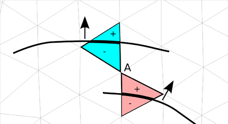
|
| Figure 8: Need for discontinuity in an embedded approach |
An obvious indicator for the distinction is again the sign of the distances that are computed. Different from before, however, the nodal distance to the structure is needed, since we want to classify each node as either outside or inside. That is basically why we need a continuous distance function instead of a discontinuous here. Details to their implementation will follow in chapter 7. For now it is only important that this distance function computes for each node a distance to the embedded structure and assigns its sign automatically according to a technique which is based on what in computer graphics is called “ray tracing”. Following this terminology the process of assigning the indicator to the single nodes is typically referred to as “coloring”
The underlying concept with this type of coloring is straightforward: Depending on an sequence of choice, different rays are “shot” through the fluid domain such that they start and end at a node which by definition lies outside. Along their way they assign every trespassed node the indication for “outside”, which we chose to be a positive sign for the respective nodal distance. Whenever a structure boundary is now crossed the rays switch their status and henceforth assign the opposite indication. So if just started the nodal distances will be tagged with a negative sign after the ray crosses a structure boundary, indicating that they belong to the interior. This is done until every fluid node was touched by a ray at least once. As a result we obtain fluid nodes that either have a negative distance to the structure, iff a fluid node is part of the structure's interior domain, or a positive distance else. Figure 9 illustrates the concept.
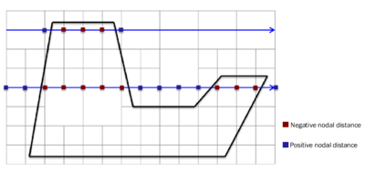
|
| Figure 9: Coloring by means of ray tracing |
Unfortunately the algorithm in its basic form only works for simple cases, excluding any model defects or similar challenges as shown in figure 10. In order to obtain a robust automatic coloring, additional implementations were necessary which will, however, not be further detailed here.
Assuming a robust coloring technique, we are finally able to apply any model assumptions to the different domains of the fluid, which are point-wise identified with positive or negative distances. Since in a lot of applications the flow in the interior is not of interest, we simply deactivate the corresponding degrees of freedom by setting all the velocities and pressures at nodes with negative distances to zero. By that the respective degrees of freedom are effectively excluded from the overall solution of the fluid.
At the end of this chapter it can be concluded: Using two different distance functions in combination with a powerful coloring technique allows to take into account both voluminous and membrane or shell structures in an embedded environment. It is worthwhile to mention that it is of no importance whether the embedded approach is applied in a CFD or an FSI context.
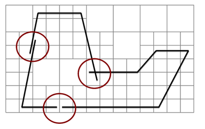
|
| Figure 10: Challenges in coloring by means of ray tracing |
2.2.4.2 Element technology
Given that the embedded structure is properly represented within the fluid domain by the techniques that were introduced in the previous section, we have to take care about the discontinuities at the embedded interface. To this end we are customizing the element formulation of the one elements that intersect with the structure. Conceptually the idea is here, to add nodes at the interface and to perform a local subdivision. Figure 11 illustrates the concept.
To introduce finally a discontinuity an obvious and easy approach might be to introduce Dirichlet boundary conditions on the newly added nodes. Unfortunately such an approach is by far not robust since the mesh obtained may become arbitrarily bad, i.e. very small and deformed elements might appear, which finally can lead to a severe ill-conditioning of the system.
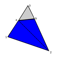
|
| Figure 11: Virtual subdivision of split element |
Therefore a different approach was chosen, instead. In there we first duplicate the nodes at the interface and divide the domain into two virtual blocks with each two virtual nodes as shown in the figure 12. Taking into account the later application we distinguish the two new virtual blocks by referring to them as each the positive or negative side of the split fluid element. As a result we may independently describe quantities on the positive side (such as a positive face pressure) or the negative side (negative face pressure), respectively.
The key idea now to solve the conditioning problem is, that instead of giving full freedom to the virtual nodes, we will express the degrees of freedom associated to those nodes as a function of the degrees of freedom of the actual fluid nodes on the respective side of the virtual domain. In our case for instance, we are imposing that the variables on the interface must respect the following constraints:
|
|
(2.33) |
and
|
|
(2.34) |
where represents any degree of freedom and the arguments correspond to the node numbers. This can be graphically understood as illustrated in figure 13.
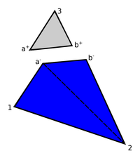
|
| Figure 12: Separation of domain by duplication of nodes |
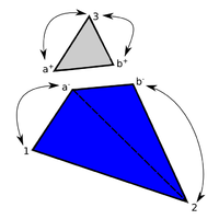
|
| Figure 13: Constraints on virtual nodes in a discontinuous element formulation |
As might be guessed up to now, an approach as described above would require a further introduction of constraints after the fluid domain was modeled with finite elements. So a better way would be to incorporate such constraints already by construction. This can now be achieved by introducing modified shape functions which indeed span exactly the same space as the one described by the standard finite element space, however, take into account the new nodes and constraints.
Functions with these characteristics were developed for other purposes in the work of Ausas et al. in [10]. The basic idea is thereby as simple as effective: The shape functions of the split fluid element are constructed in the same way as for standard finite elements, however, with the two major differences of 1) each being just defined on one of two separate virtual domains and 2) each containing a vanishing gradient along cut edges in 2D or intersecting faces in 3D. An illustration is given in figure 14.
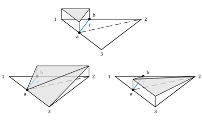
|
| Figure 14: Discontinuous shape functions |
The numerical integration over the split fluid element domain is eventually done by using the well-known Gauss-Integration method where we simply introduce separate Gauss points on each sub-triangle and integrate for each sub-triangle independently. Figure 15 highlights the idea.
Note that this is a purely local approach where the introduced auxiliary nodes on the interface are not needed, and actually not even seen in the computation of the overall system. In fact all the operations in the embedded approach are purely local with such a formulation, which is very advantageous in terms of high performance computing.
Note also that by using these modified shape functions, the finite element solution along the edges or faces that are not cut, is not changing. This is an important characteristic in that sense, that these elements can be used together with standard finite elements in a common model. As a matter of fact, the only thing that changes in the elements cut by the interface is the kinematic description used in reconstructing the different fields of interest.
Finally it is worthwhile to highlight, that by applying this modified shape function approach within an element, we introduced by construction an element that does not allow any flux over an embedded interface. That is exactly the discontinuity we wanted to implement.
Apart from this discontinuity the modified shape functions are generally continuous between elements. As will be elaborated in the later course of this monograph, however, there are “intersection patterns” in which this does not hold anymore. Anyways the hence introduced error might be still a valid approximation.

|
| Figure 15: Gauss integration in an embedded approach - The figure shows a separate integration for each sub-triangle as well as each side of the split fluid element |
2.2.4.3 Velocity boundary conditions
Because of the constraints imposed on the virtual nodes, the shape functions described above have a zero gradient in direction of each edge or face intersected by the structure. While this solves the ill-conditioning problem it implies that the gradient of the shape function normal to the embedded interface is zero. In turn this implies that if we use this modified space to describe the velocities, the only suitable boundary condition for the beginning is “slip”. How the latter is imposed in an embedded scenario is going to be explained in this section. At the end then, we will briefly sketch possibilities how a stick behavior might be introduced at embedded walls.
Given the NSE on elemental level, velocities at the embedded interface are imposed weakly by making use of a partial integration of the weighted mass conservation equation, 2.14.b. Since we have to take into account the positive and the negative side of the cut fluid element independently, we first split the integral domain into the positive and negative virtual subdomain and then perform the integration by parts. Furthermore we subdivide the generated boundary terms into the “standard” element boundaries and the embedded boundary which all together form the complete boundary of the cut fluid element:
|
|
(2.35) |
The volume integrals in here are solved using the Gauss integration for discontinuous fluid elements as described in section 2.2.4.2. The embedded boundary by contrast represents the contact to the embedded structure and is consequently constrained by the structure´s velocity. As we will see in chapter 8.3.3, it is from a practical point of view, however, difficult to introduce a corresponding constraint to the fluid formulation since in general the velocity of the structure is not constant along the embedded boundary. Therefore, in order to significantly ease the computation of the boundary integrals in 2.35, we assume that the velocity is constant along the interface within a split fluid element. This constant velocity is in the following referred to as the “embedded velocity” and it is obtained by averaging or interpolating the given velocities of the structure inside the respective fluid element. See chapter 8.3.3 for further details in this regard. Furthermore, since we regarded values along intersected edges of the fluid element as constant, as explained in the previous chapter, the embedded velocity is constant throughout the entire cut fluid element and will hence act at each fluid node equally. See figure 16 for an illustration.
Introducing this embedded velocity and having constant values along cut edges obviously makes a proper representation of the boundary layer very difficult. Apart from that, however, it has important advantages when it comes for example to the mapping of the physical quantities between the different domains, as we will see later. Since the discussed embedded method was at first not designed for an application in highly turbulent flows driven by corresponding boundary layers, and since in all other cases the boundary layer is often anyways not resolved but rather more incorporated using wall-functions, we considered this as a valid assumptions.
Introducing now the aforementioned assumptions into 2.35, we obtain for the embedded boundary in the fluid:
|
|
(2.36) |
which means that inside the cut fluid element the fluid is free to slip along the embedded boundary , but the velocity of the fluid in normal direction to the embedded boundary is prescribed by the velocity of the structure along the same direction1. This exactly corresponds to the weak form of a slip-boundary condition in a CFD simulation. It is important to note that by this approach only the part of the embedded velocity in normal direction is taken into account in the CFD solution.
We can utilize now the assumptions in terms of the constant embedded velocity to simplify the final computation of the integral from 2.36. The idea is thereby similar to the Gauss integration: We assign to each intersection node between structure and fluid (see figure 16) a part of the area of the embedded interface. Then, having assumed the velocity of the structure to be constant along the embedded interface, the computation of the integral reduces to a simple multiplication in the form:
|
|
(2.37) |
where describes a fraction of the overall area of the embedded boundary at the intersection node . is here computed by means of weighting the overall interface area which in turn relies on simple geometric considerations. As already pointed out, this way of computing the integral is of course just valid under the assumption of a constant embedded velocity.
At this point the two major approximations that were introduced and discussed in the course of this section shall be recapped briefly:
- So far in the embedded approach we assumed by construction a slip boundary condition along the interface of the embedded structure
- We considered the velocity of the structure to be constant within a single cut fluid element.
These are clearly assumptions that will lead to approximation errors. Their actual influence has to be tested, though. First investigations to this end will follow in subsequent chapters. Here it shall only be emphasized that, while the errors introduced due to the second assumption are becoming negligibly small as refining the background fluid mesh, errors due to a restriction to slip-conditions do not. An implementation of stick-conditions in the given embedded approach is, however, still part of ongoing developments, which is why at the end of this section only the principal idea of the main approach in this context shall be sketched.
A stick boundary condition may be introduced in the form:
|
|
(2.38) |
where is the orthogonal distance to the wall. The latter may be computed from geometric considerations that can be done once the embedded structure is mathematically captured by the distance function. Given that , a simple wall law might read:
|
|
(2.39) |
where we introduce a pseudo viscosity in that sense that we apply a prescribed velocity in opposite direction to the given velocity field at the embedded boundary. The concept is illustrated in figure 17. This procedure of introducing wall laws within cut elements is in fact very promising and might be further exploited in future developments. The objective should be to enrich the embedded approach with powerful wall-laws in order to be able to sufficiently represent the boundary layer.
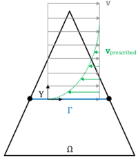
|
| Figure 17: Introduction of a wall law to allow for stick boundary conditions on an embedded interface |
2.2.4.4 Pressure boundary conditions
Having applied a velocity boundary condition of Dirichlet type at the embedded interface within a cut fluid element in order to incorporate the movement of the structure, the fluid at the interface immediately reacts to this by adjusting the pressure on the interface such that there is no flux through it, i.e. the discontinuity requirement is maintained. This pressure change in turn has to be applied as Neumann BC on the remaining fluid domain. Classically this can be done either in a strong or in a weak from, respectively. Therefore we recap the pressure term from the weighted NSE given in equation 2.13.a:
|
|
(2.40) |
Partial integration of this term yields:
|
|
(2.41) |
In principal this equation offers now two possibilities: Either we prescribe the pressure in a strong form by inserting it on the left hand side of the equation and use the latter in the computation of the NSE, or we use the partial integrated formulation on the right hand side and hence impose the pressure in a weak form by introducing a traction in the respective boundary term such that we get a total of
|
|
(2.42) |
where describes the Neumann boundary. Note that we are changing by this the continuity requirements with regards to the pressure. I.e. while the pressure needs to be continuous in 2.40 it can be discontinuous in 2.42, which clearly relaxes requirements in terms of the solution space. So with the computation of the NSE, we have to choose between either using the strong formulation given in 2.40 or the weak formulation with relaxed solution requirements given in 2.42.
Knowing that the fractional step method we are using is generally based on a strong imposition of pressure boundary conditions, we chose to apply pressure boundary conditions at the embedded interface in a strong form. By that we are increasing the accuracy2 whereas at the same time lowering the computational effort 3. It shall nevertheless be emphasized that this win-win kind of situation is only given with the fractional step method and may look different in other cases in which a weak imposition of the pressures boundary conditions might be inevitable. In the framework of the given embedded method, though, this means: Pressures at embedded interfaces are imposed strongly in the form of 2.40.
(1) Note in this context the scalar multiplication of with the boundary or structure normal
(2) Since we are fulfilling the pressure boundary condition point-wise
(3) Since we are not forced to compute additional terms as they occur in a weak formulation
2.3 Computational structure mechanics
In the framework of this chapter a very basic but general overview is given about the differential equation of an elastic solid and its discretization in space and time. An extensive introduction into the topic is given in Malvern [2], Holzapfel [11] and Belytschko [12]. A further very recommendable work in this context is the classical textbook on FEM by Zienkiewicz [13].
2.3.1 Governing equations
As already mentioned in table 1 the structure is mainly described by a Lagrangian description of motion. Based on this approach we will discuss the main equations in the following. This will finally lead us to the initial boundary-value problem of elasticity theory.
Kinematics
Considering a deformed body in the current configuration - expressed by the coordinates - it can be related to the reference configuration by means of the displacement field at any point of time:
|
|
(2.43) |
Accordingly, the velocity field of the material particles can be derived
|
|
(2.44) |
as well as the acceleration field
|
|
(2.45) |
In order to describe the relation between both configurations, the deformation gradient as a fundamental measure in continuum mechanics is introduced
|
|
(2.46) |
and therefore represents a mapping function of a line element in the reference configuration to the current configuration. As the deformation gradient is not suitable as strain measure, the non-linear Green-Lagrange strain tensor is introduced which is applicable for large deformations and equals to zero in an undeformed state
|
|
(2.47) |
whereas denotes the unit tensor. From the equation it appears that the Green-Lagrange strain tensor refers to the undeformed configuration. There is also other strain measures such as the Euler-Almansi strain tensor which refers to the deformed configuration and contains the inverse of .
Balance equations
The inertia forces, internal forces as well as the external forces reacting on a body in the current configuration are in equilibrium according to Cauchy's first equation of motion (balance of linear momentum):
|
|
(2.48) |
Here, denotes the material density in the current configuration, the Cauchy stress tensor and an acceleration field characterizing the external force. This field equation is stated in strong or local form indicating that it is fulfilled at any point throughout the current domain . As we want to refer the set of equations to the reference configuration in the manner of the Total-Lagrangian formulation, the equilibrium equation can be transformed to reference configuration. To this end, the Cauchy stress tensor has to be rewritten with regard to the reference configuration resulting in the second Piola-Kirchhoff stress tensor :
|
|
(2.49) |
Then, the balance of linear momentum w.r.t. the reference configuration can be formulated as
|
|
(2.50) |
in which we use the material density in the reference configuration. The external volume body force is now considered to be a function of the reference configuration
|
|
(2.51) |
The aforementioned symmetry of the second Piola-Kirchhoff stress tensor is particularly expressed by Cauchy's second equation of motion (balance of angular momentum)
|
|
(2.52) |
which is also valid for the Cauchy stress tensor
|
|
(2.53) |
For the sake of completeness, we also want to mention the mass balance equation
|
|
(2.54) |
at which characterizes a measure for the volume ratio of infinitesimal small volume elements in an undeformed and a deformed configuration.
Constitutive equations
The constitutive equations manifest a relation between the stress and the strain measure and thereby linking the reaction of the material to the applied loads. In the course of this work we will use materials which allow large displacements but small strains, what advises to use the St. Venant-Kirchhoff material model resulting in a linear relationship between the Green-Lagrange strain tensor and the second Piola-Kirchhoff stress tensor
|
|
(2.55) |
whereas describes the elasticity tensor of fourth order. Further assuming an isotropic elastic material, the stress-strain-relationship can be resolved to the following equation
|
|
(2.56) |
at which and are the Lamé constants which depend on the material specific Young's modulus and Poisson coefficient . In problems witch small deformations, the difference between the deformed and undeformed configuration can be neglected such that the constitutive equation reduces to
|
|
(2.57) |
what describes a linear elastic material behavior. Therein, denotes the linear elastic strain tensor.
Initial boundary value problem
The kinematic relation 2.47, the balance of momentum 2.50 and the constitutive equation 2.55 hold throughout the entire domain which is initially defined by a prescribed displacement field and velocity field
|
|
(2.58) |
The domain is limited by the boundary along which the boundary conditions have to be defined for any point of time. At every location of the boundary either the state variables itself have to be prescribed (Dirichlet boundary conditions) or their derivatives (Neumann boundary conditions)
|
|
(2.59) |
|
|
(2.60) |
The normal vector denotes the vector normal to the Neumann boundary. and are non-overlapping and jointly cover the complete boundary .
2.3.2 Discretization
Generally the strong form of the momentum balance can not be solved analytically which requires to use discretization techniques in order to find an approximate solution. This section discusses the applied methods for the discretization in space and time.
2.3.2.1 Spatial discretization
The method of Finite Elements is used for spatial discretization. The idea is to introduce a finite number of nodes throughout the domain at which the displacement field is approximated. The field in between the nodes is described by an interpolation by means of shape functions, e.g. Lagrange polynomials. The Finite Element method does not solve the strong form but the weak formulation of the differential equation which can be derived by integral principles, more precisely the principle of virtual work. This principle states that if a domain is subjected to an admissible, infinitesimally small virtual displacement , the generated virtual work has to vanish (i.e. ).
The application of the principle of virtual work to the strong form 2.50 leads to the following equation in Total-Lagrangian formulation in which the structure is considered w.r.t. the reference configuration (characterized by the undeformed domain and the undeformed boundary )
|
|
(2.61) |
with
|
|
(2.62) |
|
|
(2.63) |
|
|
(2.64) |
This set of equations expresses that the sum of virtual work of inertia forces , internal forces and external forces vanishes.
Introducing the concept of Finite Elements, the displacement as well as the material coordinate at any location within an element can be described with the matrix of shape functions based on the nodal displacements :
|
|
(2.65) |
Based on this approximation, the strain-displacement relation can be written, assuming small deformations and rotations (derived from equation 2.47)
|
|
(2.66) |
whereas is the strain-to-displacement differentiation operator, which can be reviewed in the recommended literature, and denotes the strain-displacement matrix. Substituting these equations into the weak form we finally obtain for an arbitrary finite element in the Total-Lagrangian formulation
|
|
(2.67) |
|
|
(2.68) |
In an Updated-Lagrangian formulation, which considers the system in the deformed state, the shape functions are a function of the current configuration . Further, the integration has to be performed over the current domain and the current boundary :
|
|
(2.69) |
|
|
(2.70) |
The integration on element level is usually approximated with the Gaussian quadrature (see e.g. [13]). Taking the sum over all elements we will end up in the semi-discrete problem [13]
|
|
(2.71) |
with
|
|
(2.72) |
where is the quadratic, symmetric and sparse mass matrix, the internal force vector and the external force vector.
2.3.2.2 Time discretization
The time discretization is performed with a second order Newmark-Bossak scheme, [14], which shall be shortly introduced here. We want to concentrate on the Updated-Lagrangian formulation in which the reference configuration is updated at each time step. Therefore we can compute the current configuration at time step based on the reference configuration at time step .
In the Newmark scheme [15] the set of unknown variables in equation 2.71 is reduced to the displacements which implies that the velocity and the acceleration have to be expressed as functions of the displacements in time step :
|
|
(2.73) |
|
Here, and and are constants which control the order of accuracy and numerical stability and can be chosen e.g. according to [15]. Inserting equation (2.74) into the semi-discrete differential equation (2.71) yields
|
|
(2.75) |
in which the internal force vector is typically given in the form
|
|
where is the global stiffness matrix. Equation (2.75) is a non-linear equation system for the unknown displacements which can be solved in an iterative solution procedure using e.g. the Newton-Raphson method.
3 Fluid-structure interaction
Up to now we considered structure and fluid to be independent and restricted ourselves to their single field solution. In engineering practice, though, both mechanical systems are often tightly coupled and hence need to be combined in a global model whose interaction may be simulated by means of dedicated solution procedures. Nowadays, as a result of intense research and development during the last decades, powerful and efficient technologies are available therefore making it more and more attractive to incorporate different interaction phenomena in the classical single field analysis. The expectation here is to be able to get a more profound understanding of complex fluid-structure systems in which the coupling plays an important role, such as for instance light-weight structures in a CFD context. This chapter now shall provide the relevant theoretical background for such a coupled fluid-structure analysis.
The chapter is organized in three different parts. In the first part the coupling conditions are introduced, so it will be briefly discussed what it formally means to couple a fluid- with structure-mechanical problem. In the second part then different possibilities for the mechanical formulation of the global FSI-problem shall be presented. At this point indeed a brief overview of possible approaches will be given, but general focus will be the embedded and the Arbitrary Lagrangian-Eulerian approach. Finally relevant solution procedures will be discussed in more detail. To this end both the monolithic and the partitioned approach shall be discussed together with the question of how to get from the system in the first approach to the one in the latter as well as what possibilities and drawbacks either way has got. Focus here will be the partitioned approach. In this context the numerical problems related to the artificial added-mass effect will be introduced for which at the end of the chapter a stabilization method will be presented.
3.1 Coupling conditions of the FSI problem
In the previous chapter the fluid as well as the structure have been considered as separate fields which do not interact with each other. In order to take a strong coupling between the fluid domain and the structure domain into account, the coupling conditions at the coupling interface, which is defined as the shared boundary , have to be fulfilled. The notations can be taken from the visualization in figure 18.
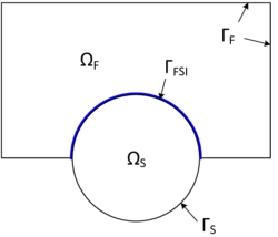
|
| Figure 18: FSI coupling interface - The fluid domain with the boundary and the structure domain with the boundary share the FSI interface . |
On the one hand, the particles are not allowed to cross the shared interface which enforces a kinematic condition depending on the applied fluid model [5]. In case the viscosity of the fluid cannot be neglected (viscous fluid), a "no-slip"-condition at the interface can be defined as follows
|
|
(3.1) |
|
|
(3.2) |
These equations express the continuity of displacements and velocities across the interface. Physically it means that the fluid particles close to the interface conduct the same movement as the particles on the structure domain. Depending on which formulation and therefore which coupling variable is chosen (displacement or velocity), only one of the two equations is applied as they are equivalent in their physical meaning. If viscous effects of the fluid can be neglected, a "slip" condition needs to be defined instead. This results in the following relations
|
|
(3.3) |
|
which describes the continuity of displacements and velocities perpendicular to the interface.
On the other hand there are dynamic conditions which the fluid and structure have to comply to at the interface:
|
|
(3.5) |
These conditions guarantee that the force equilibrium of the surface traction vectors along the interface is fulfilled.
3.2 Formulation of the FSI problem
A key question in approaching FSI problems is the question about how to formulate the material motion in the fluid and the structure field. In the last decades many different formulation methods have been proposed of which each has advantages and drawbacks when applied to certain physical problems. In the framework of this monograph we will focus on the fundamentally different ALE method and embedded method. However, in the first part of this chapter we want to relate these methods to a very general context of FSI formulation methods. Afterwards, the ALE approach will be further discussed in detail, whereas the embedded method was already treated intensively in chapter 2.2.4.
3.2.1 Two principal formulation methods
A very detailed and widespread overview about formulation methods in general may be found e.g. in [16], [17] and [18] as well as in the included literature references.
To explain two principal formulation methods, let us first of all assume a rigid body motion of a structure within a discretized fluid domain (See figure 19).
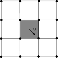
|
| Figure 19: Rigid body motion of a structure (grey) in a fluid domain |
A classical way to handle the coupled motion is by using a body-fitted solution approach in which the fluid nodes at the FSI interface are forced to follow the movement of the structure at the same interface (See figure 20).
This is done in the so-called Arbitrary Lagrangian-Eulerian (ALE) method [5,19]. The ALE method has many advantages making it the method of choice for many applications. It allows for example an easy tracking of the FSI interface and therefore provides high accuracy of the flow along the interface. This may result in a high overall accuracy of the solution. Even cases in which the grids of the fluid and the structure along the interface do not exactly match can be handled. Therefore mapping techniques are used which in general allow to map quantities between arbitrary different grids. Throughout the present work we therefore use the Mortar Element Method described in [20].
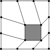
|
| Figure 20: Body-fitted solution approach |
On the other side, however, it is possible in an ALE approach, that large deformations and rotations distort the mesh such that even a costly remeshing may become necessary. In fact this typically happens when simulating the previously introduced inflatable hangar. Here the problem becomes even more critical since the structure starts to wrinkle or fold as indicated in figure 21.
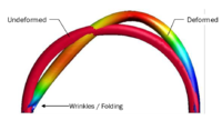
|
| Figure 21: Folded tube of an inflatable hangar structure - If the hangar is subjected to severe wind loads, the tubes may be massively deformed resulting in such a wrinkling and folding. |
In order to treat large deformations or such complex movements, one can apply non-body-fitted or fixed-grid methods in which the fluid mesh remains unchanged. The fluid domain is then described by an Eulerian formulation and the structure moves independently from the fluid nodes locations. The concept is visually explained in figure 22.

|
| Figure 22: Embedded approach - The fluid and the structure mesh are completely decoupled from each other. |
A widely used method based on the fixed-grid approach is the embedded or immersed boundary method which was first proposed by Peskin [21,22] in order to simulate the blood flow through a beating heart. Initially used with Finite Differences, it was later extended to Finite Elements as the Immersed Finite Element Method, e.g. by using the discrete Dirac delta functions [23]. Another derived method is the Fictitious Domain Method discussed e.g. by Glowinski et al. [24] which describes the interface between fluid and structure by means of a distributed Lagrange multiplier. An extension of the fixed-grid approach to the application of compressible solids and fluids is provided by the Immersed Continuum Method (see also [25]). A general overview on the derivations of Immersed Boundary Methods is e.g. given in [26]. It is important to realize that with all immersed methods the solution accuracy or stability depends on the given background mesh which typically is seen as a big disadvantage.
Finally, the advantages of the ALE- and the embedded method can be combined in Chimera method which divides the fluid into a moving domain around the FSI interface and a non-moving domain further away from the interface. An example where the Chimera method was successfully applied with flexible structures is given in [27].
In the following the ALE method is discussed on a more theoretical basis. The theoretical background of the embedded method is given in chapter 2.2.4.
3.2.2 Arbitrary Lagrangian-Eulerian Method
The purely Lagrangian description of the fluid domain has the disadvantage to result in locally strong mesh distortions with increased motion of the FSI interface. Having this in mind, the goal of the ALE method is to let the fluid nodes move "arbitrarily" in a Eulerian manner such that the distortions of the elements in the fluid domain are minimized and larger structural deformations are possible. Therefore, the advantages of Lagrangian and Eulerian methods are combined (consider also the overview in table 1).
The ALE method was first applied to FEM by Donea, [3,5], whose papers are a recommendable guideline to understand the algorithm in detail. As opposed to the Lagrangian and Eulerian description of motion, the idea of the ALE method is to introduce a third domain, i.e. the mesh domain. The latter is the so-called referential configuration with the corresponding referential coordinates describing the motion of the mesh points. The velocity of the grid points can be hence be computed as
|
|
(3.6) |
Based on the mesh velocity we can introduce a new measure which characterizes the relative velocity between the mesh and the material points, i.e. the convective velocity :
|
|
(3.7) |
Using the convective velocity we unify the Lagrangian and Eulerian description in an ALE formulation by reformulating the material derivative (see equation 2.4) such that it refers to the additionally introduced referential (mesh) configuration:
|
|
(3.8) |
whereas can be e.g. the fluid particle velocity . Based on the adjusted material derivative, the momentum equation of the Navier-Stokes Equations (2.10.a) can be rewritten as
|
|
(3.9) |
in which we replaced in the convective term the material velocity by the convective velocity. Equation 3.9 represents the ALE-formulation of the Navier-Stokes Equations.
Finally, the aforementioned "arbitrary" movement of the mesh points at each time step requires certain so-called mesh-updating strategies which distribute the interface deformation over the fluid domain. Many approaches have been proposed to this end, whereas two main strategies can be identified: mesh-regularization and mesh-adaption [5]. Herein, we will concentrate on strategies based on mesh regularization. A very straight-forward approach in this context is to handle the movement of the FSI interface by solving a second-order partial differential equation. Prominent examples are the springs algorithm (see e.g. Farhat [28]), the elastic deformation method (e.g. Baker [29]) or solving a Laplacian equation based on the interface movement, which goes back to the work of Winslow [30]. The specific algorithms we use throughout this work are described in chapter 8.2.1.
3.3 Solution of the FSI problem
In the previous chapter the formulation of the FSI problem was discussed. With that in mind this chapter now aims to provide the theoretical background in terms of the corresponding solution procedure. To this end we will in the first section discuss the two main solution approaches, i.e. the monolithic and the partitioned or staggered solution. Since we are in the course of this monograph only applying the partitioned approach, we will here mainly focus on the latter solution technique. A detailed description of how to actually reformulate the system to obtain a partitioned solution process is therefore presented. In the second part of this chapter then we will concentrate on one of the most important numerical problems related to the partitioned FSI analyses, i.e. the artificial added-mass effect. This will be important for the interpretation of the results later. Finally a stabilization technique shall be presented which allows to effectively use the partitioned analysis for strongly coupled problems.
3.3.1 From the monolithic to a partitioned solution
This section will introduce the theoretical concepts in terms of the numerical treatment of FSI-problems. In doing so we will mainly rely on the very detailed elaborations in [31], [6], [32],[33] and [34], to which the interested reader shall be referred to for further information. Distinct focus will be set on techniques to establish a fully partitioned solution scheme based on a Dirichlet-Neumann coupling. Even though the formulation of the underlying mechanics as well as the corresponding concepts are introduced in a very general manner, no attempt will be made to cover the full spectrum of possible solution procedures. A very nice and profound classification of the latter, though, can be found in chapter of [31].
From a mathematical point of view an FSI problem can be expressed through an ODE system in the form1
|
|
(3.10) |
where , and characterize the motion of either the fluid or the structure , the coefficient matrix describes the mass, the damping and the stiffness of the system. Furthermore denotes the right-hand side that contains the sum of all imposed forces. The actual coupling between both domains is herein given by the off-diagonal or mixed terms indexed with or .
If all the matrices are now fully occupied one speaks of a fully coupled or two-way coupled FSI-problem. Here we may distinguish between two different situations: strongly coupled systems in which the density ratio between fluid and structure is , and weakly coupled systems where the respective density ratio is . This distinction is important with regard to the choice of the solution procedure.
If in either of the two lines of the above system the mixed terms are missing a one-way coupled system is obtained and finally if no mixed-terms are present the two systems are fully decoupled and could be solved independently.
Given a fully coupled FSI problem and assuming that all the corresponding coefficients in 3.10 are known, the ODE system can be directly discretized in time leading to the so called “monolithic” formulation of the coupled problem. In that configuration the complete problem can be solved for the state variables conveniently in a single solution step by means of an arbitrary integrator for ODE-systems, which is very advantageous from the point of view of accuracy. This solution procedure is in the following referred to as the monolithic solution.
The disadvantage of a monolithic solution procedure is, however, that the corresponding system of equations is generally very large (all the variables of the problem need to be solved at the same time) and often badly conditioned due to the coexistence of terms coming from the description of physically different problems [6]. To overcome these disadvantages it is possible to split the monolithic system into the two single field problems such that they indeed take into account contributions from each the other field at the common boundary or interface, respectively, but apart from that can be solved independently. As we will see later, the solution then follows a defined strategy which is based on a mutual exchange and imposition of boundary conditions at the common interface.
The underlying formulation of such a partitioned solution procedure is obtained by bringing all the coupling quantities in equation 3.10 to the right hand side. The system then reads:
|
|
(3.11) |
in which
|
|
(3.12) |
This system of equations may be eventually solved in a partitioned manner.
Besides the fact that we are avoiding the complications related to a monolithic solution, this partitioned solution procedure offers a few more very nice advantages. The most important one is the fact that from a solution perspective the two different mechanical problems are decoupled. That is optimal from the point of view of software modularity since for either problem we can use dedicated and well-established high-performance solvers. The disadvantage, though, is obviously the additional computational effort. Since we are solving each system independently, we need make sure that in each time step the coupling conditions are fulfilled to a high degree of accuracy in order to keep the accumulated error minimal. This requires an additional solution iteration in each time step and hence causes a significant increase in the number of solver calls. Another typical disadvantage arises from possible convergence problems during the additional solution iteration. Also it may happen that the problem is not well defined on one of the domains since boundary conditions are only defined in the other domain2. In a lot of applications, though, the advantages of this approach outweigh the disadvantages making it a frequently applied solution approach in the context of FSI simulations.
Nevertheless, the feasibility of such an approach relies on the following three assumptions [6]:
- the system (equation 3.10) is linear
- the corresponding matrix coefficients are all known
- it is possible to define physically stable test case
For a detailed discussion of the latter assumptions the interested reader is referred to chapter page in [6]. At this point it is only important to note, that in case of the interaction between flexible structures and incompressible fluids, which is the system of interest within this monograph, none of the previous assumptions are valid[6]. This leads particularly in situations where , i.e. in strongly coupled problems, to numerical difficulties. One such difficulty is the artificial added-mass effect described in the follow-up section.
To overcome these problems two principal solution or coupling strategies may be applied in partitioned analyses3:
- an explicit computation with prediction-correction techniques
- an iterative or implicit solution procedure
In the first case the single field problems are solved subsequently just once in each time step. Therefore typically information from the previous time step is used as a prediction. In order to reduce the hence occurring spurious energy, additional correction techniques may be applied. Given a very weak coupling, i.e. , the solution of the system formulated in equation 3.10 can be simplified even more since then it can be solved in a purely explicit manner without correction. A purely explicit computation is the fastest way to obtain a coupled solution in the context of a partitioned FSI analysis. In practical applications, however, it is typically either not sufficient or not applicable. Since in the scope of this monograph we are exclusively relying on the second of the above principal coupling strategies, details are omitted here. Instead the simple but complete example from chapter 2.1.1 in [34] shall be recommended. It describes the algorithmic idea of the partitioned analysis4 by means of an explicit computation with prediction-correction techniques which may serve as a basis for further research in this context.
In case of the second solution strategy, iterative schemes are applied to control numerical problems in a coupled analysis. The basic idea in this context is an implicit treatment of the coupling variables where in each time step the latter are iteratively improved until the residuum, defined by the the coupling conditions, is below a certain tolerance threshold. Then one proceeds in time starting with the iteration all over again[31]. An illustration of the implicit solution procedure is given in figure 23.
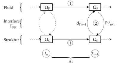 ] ]
|
| Figure 23: Iterative solution procedure - Adopted from [31] |
Important to note is that by using such a solution approach, the coupling conditions are fulfilled (up to the degree of accuracy defined by the tolerance threshold) and the energy conservation at the common interface is ensured. An implicit solution of equation 3.11 following the procedure above hence principally convergences to the monolithic solution of equation 3.10 (Given that it converges at all) [31], which has to be an essential characteristic of a partitioned approach in general. In order to actually allow for convergence, though, we have to follow one of several possible iteration schemes. Throughout the present monograph the so called “Gauss-Seidel” fixed-point iteration scheme was chosen to this end. The reason for this choice was the existing profound experience basis in this regards.
The Gauss-Seidel fixed-point iteration aims to iteratively solve the constrained nonlinear FSI problem from equation 3.11 assuming that the sought equilibrium condition appears as a so called fixed-point5 in the solution space. The corresponding iteration rule then requires to reformulate 3.11 such that we obtain its corresponding fixed-point form:
|
|
(3.13.a) |
|
|
(3.13.b) |
where is the iteration index. Now we recap that at the interface it holds:
|
|
(3.14) |
Using 3.13 and 3.14 the iteration rule of the Gauss-Seidel fixed-point iteration finally reads
- Given from the previous time step or iteration, solve the structure problem in 3.13.a for
- Use the coupling conditions in 3.14 to prescribe the solution quantities at the interface on fluid side.
- Solve the fluid problem in equation 3.13.b for the remaining solution quantities on fluid side. Then restart iteration.
According to Banach's fixed-point theorem this iteration now converges under the condition that each single iteration step mathematically corresponds to a contraction. The latter condition, though, is not always fulfilled and typically violated in strongly coupled problems, which we actually wanted to solve with the introduced iterative scheme. To make sure that the contraction condition remains valid along the iteration, however, we can use a relaxation method which relaxes either of the coupling variables at the interface during step 2) in the above iteration rule. The corresponding relaxation generally reads:
|
|
(3.15) |
|
|
(3.16) |
where represents the relaxed coupling variable, the unrelaxed variable, denotes the iteration index and the relaxation factor. In the specific case where the structural velocity is relaxed, as we will do it later, step 2) in the above iteration reads:
|
|
(3.17) |
This means, that we are in each iteration step not imposing the actual simulated value for the structural velocity on the fluid boundary at the common interface, but only an, according to , relaxed value, which is typically smaller than the original one. That is the relaxation factor is typically chosen which corresponds to an underrelaxation. Practically interpreted this means that we are relaxing the load with which the structure excites the fluid in each iteration during one time step. Conceptually we are by that ensuring a contraction in the fixed-point iteration. As a result convergence of the fixed-point iteration may be achieved even with strongly coupled problems. The fixed-point iteration scheme combined with the above described relaxation method hence poses a powerful solution procedure that also allows a partitioned analysis of strongly coupled problems.
Even though this is a very powerful approach, the question remains, how to choose . Generally it holds that the corresponding value needs to be as low as possible to actually achieve numerical stability but high enough to reduce the hence increasing number of necessary iteration steps as much as possible. In practice this trade-off often cannot be effectively balanced out by the program user himself. Instead automatized strategies to accelerate convergence can be applied. A very effective and important strategy in this context is the adaptive relaxation using the Aitken-method which during the iteration continuously computes new and improved relaxation parameters. A detailed elaboration of this method including its computation as well as background information can be found in [31], chapter and the herein given references. Throughout this monograph the above discussed Gauss-Seidel coupling strategy is combined with the aforementioned Aitken-method in order to ensure convergence.
With the Aitken-method now we discussed all the principal theoretical concepts regarding the solution of a coupled fluid-structure problem that will be of importance in the later course of this monograph. As already stated in the beginning we in particular focused here on a partitioned solution procedure. What in this regard was already mentioned but not elaborated further so far is the fact that a partitioned approach typically faces well-known numerical problems, which has to be taken into account in a proper simulation. One of the most important problems shall be discussed in the following section.
(1) Here we already discretized in space via the finite element method
(2) Pressure boundary conditions on the structure are actually defined in the fluid domain
(3) A profound overview of different coupling strategies, in particular for the second case, is given in [31], chapter
(4) In [34] denoted as the “staggered approach”
(5) See respective mathematical textbooks for a definition
3.3.2 Artificial added-mass effect
Whenever acceleration is imposed on a fluid flow, either by accelerating an embedded body or by an external acceleration of the fluid, additional inertia forces will act on surfaces of embedded bodies that are in contact with the fluid [35]. This effect is typically referred to as the “artificial added-mass effect”. For a simple voluminous, spherical particle embedded in an incompressible fluid domain for instance the additional inertia force, also referred to as the virtual mass force, is given as [36]:
|
|
(3.18) |
where is the fluid flow velocity, is the spherical particle velocity, is the mass density of the fluid, is the volume of the particle, and denotes the material time derivative. Taking into account the aforementioned virtual mass force, the momentum equation of the particle for example reads:
|
|
(3.19) |
in which represents the mass of the particle and contains all the imposed forces like the gravitational force, drag, lift, Basset force, etc.. By rearranging the equation we get:
|
|
(3.20) |
In front of the first order time derivative of the particle velocity now an extra mass term occurs that arises due to the interaction of the fluid with the particle or the structure in general. That is, the particle accelerates as if it had an extra mass of half the fluid it displaces. This extra term is typically referred to as “artificial added-mass” or simply “added-mass” giving this effect its notion. The particle is now just an example, but the effect is conceptually the same in the general case. A mathematically more rigorous derivation for the general case is given in [37].
As already stated in the beginning, the artificial added-mass effect affects the surface of the structure that is in contact with the fluid. Transferred to the case of a partitioned FSI analysis the effect hence exclusively occurs at the coupling interface. Furthermore it is important to realize that, since we are in an FSI analysis generally dealing with transient movements, the artificial added-mass effect is always present. Its impact depends, however, on the density of fluid. If the fluid density is small compared to the density of the structure it can typically be neglected. In cases where the density of the fluid is about the density of the structure or higher, the added-mass may be even greater than the mass of the structure itself so the corresponding effect has to be taken into account. Severe numerical errors might be the consequence else. A typical error that is seen in this context, is for instance a pressure distribution that is significantly oscillating in time.
The effect is particularly a problem in fluid-structure scenarios with incompressible fluids at a density ratio of . Here the resulting inertia terms may dominate the solution of the interaction problem. On the other hand side the effect generally diminishes in an analysis with compressible fluids. This can be understood with a rather practical interpretation of the artificial added-mass effect: Since fluid and structure cannot occupy the same space at the same time the structure displaces the fluid as it accelerates through it. The fluid reacts to it with an additional inertia response, that in turn is all the more distinct the higher the effective mass of the fluid, i.e. the one partition of the entire fluid mass that immediately reacts to this state change. In compressible fluids obviously the effective mass is significantly lower than in incompressible fluids where, due to the incompressibility constraint, the entire mass of the fluid reacts to this state change at once.
In partitioned FSI analyses the artificial added-mass effect and the possible numerical errors are typically handled very effectively by means of implicit coupling strategies. As we will see later, however, this might be still not enough in terms of the herein discussed embedded method. In this case additional techniques are necessary in order to prevent numerical instabilities. A corresponding technique that was applied throughout this monograph will be introduced in the following section.
3.3.3 Dealing with the artificial added-mass effect in incompressible flows
In the previous chapter we described a particular problematic phenomena when computing an FSI scenario with incompressible fluids in a partitioned approach, i.e. the artificial added-mass effect. One typically very efficient way to avoid this phenomena is to use an implicit, iterative solution procedure with corresponding relaxation technique as described in the first part of this chapter. Despite the application of the latter, however, it could be observed with the herein given examples, that in particular the embedded method still is prone for instabilities due to this artificial added-mass effect, given that we have a density ratio close to one. So in order to prepare the embedded method also for problems of the latter kind it was necessary to improve the stability of the partitioned embedded solution procedure.
In order to understand where there is actually potential for an improvement we recap the origin of the problem with the artificial added-mass effect from a more pragmatic perspective: The problem is, that we do not incorporate any sensitivity information so far into the analysis of the fluid-structure interaction since the computation of the corresponding derivatives is very expensive. That is whenever we compute the solution of the fluid as a reaction to the movement of the structure we do actually not take into account that the hence resulting pressure variation has an influence on the movement again. In turn, to be more precise we would have to incorporate the sensitivity of the structural movement w.r.t. to a pressure variation into the analysis of the actual pressure variation on CFD side. By neglecting this, it is essentially assumed that the structure and the fluid may partially overlap during the iteration from one time step to the other. This is of course contrary to the original assumption of incompressibility which eventually leads to pressure-oscillations or this artificial added-mass, respectively. So the general idea is now to incorporate into the analysis of the fluid this missing information about the structural response if there is a pressure variation at the interface (This approach partially follows the ideas presented in [38]). To incorporate the missing information, we have to perform two basic tasks:
- Find a sufficient prediction of the structural response and
- incorporate this prediction into the fluid analysis.
Let us first concentrate on the linearized prediction of the structural movement. In order to keep it simple here we will in the following derive the necessary equations on a discrete level which is based on a standard Galerkin weak form analysis. With that in mind, consider the case of a general structural problem in the form
|
|
(3.21) |
where we used the same notation as in the previous chapters and comprised all the external forces in one vector . Introducing a first order backward-Euler time-integration this can be further discretized in time as
|
|
(3.22) |
where and denote the current and following time step, respectively. Having introduced the time discretization we may reformulate the problem such that we have an expression which approximates the structural movement as
|
|
(3.23) |
Now we note that the displacement is proportional to the time step , i.e. . That is as the time step reduces the second term with the tangential stiffness in the equation above decreases second order while the first term depending on reduces linearly. Taking now into account that this stabilization is to be applied in strongly coupled problems where typically very small time steps are required, we may neglect the influence by the tangential stiffness as since the structural behavior is mainly dominated by the inertia term. Equation 3.23 reduces to
|
|
(3.24) |
Note that this is a clear simplification but as we will see later it is sufficient for a proper stabilization. Introducing now an iterative solution technique with iteration index the solution for this equation at two subsequent iteration steps reads1
|
|
(3.25.a) |
|
|
(3.25.b) |
Subtracting now equation 3.25.a from 3.25.b and rearranging the resulting term we get a linearized Newton-Raphson solution scheme to solve for the structural velocities depending on the external forces:
|
|
(3.26) |
Now we note that, by choosing a weak formulation and the Galerkin discretization, the external force vector is decomposed into body forces and surface tractions along the Neumann boundary:
|
|
(3.27) |
where is the body force and the surface traction that may be given as a surrounding pressure field in the form
|
|
(3.28) |
with being the surface normal at the coupling boundary. Introducing 3.28 in 3.27 and the latter into 3.26, the final structural movement may be written as
|
|
(3.29) |
Note that by these operations we obtained an expression that not just describes the reaction of the structure to any body load, but also an expression that takes into account a pressure variation along the Neumann boundary. Practically interpreted this means that, given a pressure variation from any environmental phenomena, such as a surrounding fluid, its influence on the structural movement may be described by the boundary term
|
|
(3.30) |
The information from the above boundary terms can now be used to improve the fractional step solution procedure when computing the fluid in a partitioned FSI problem. Before entering the term, however, in the fractional step process, we want to prepare it some more.
First we note, that the pressures in an FSI context are nodal quantities which is why we also need to discretize them by means of finite elements. Taking the latter into account we can reformulate equation 3.30 to
|
|
(3.31) |
where the pressure values are now nodal quantities interpolated via the additional shape function . The integral can now be computed by means of Gauss-integration techniques. Here all the constant terms were put outside the integral.
Second we note that in the FSI context the boundary along which the pressure variation needs to be taken into account is the common interface or “wet” interface , respectively. We may thus want to make this clear by denoting the boundary term as
|
|
(3.32) |
Also we want to emphasize for the later application in the FSI that the above mass matrix describes the nodal masses at the boundary of the structure by replacing with :
|
|
(3.33) |
Third we note that the mass matrix is composed of the structural density and the nodal volumes assigned to each node on the boundary. By contrast the integral poses a nodal area which represents the area of influence of each node along the boundary. Assuming a nodal integration rule, both are hence of the form
|
|
(3.34) |
|
Considering now that the nodal volume of an interface node divided by the corresponding nodal area results in some nodal thickness description, i.e. , what remains from the multiplication of both matrices in equation 3.33 is a coefficient matrix in the form
|
|
(3.36) |
We can hence rewrite 3.33 such that we have
|
|
(3.37) |
A few important observations can now be made here. For example as increases, this term tends more and more to zero, which when applied in the FSI context is what we expect since for heavy structures its movement will be less influenced by a surrounding fluid. That is, this term has a negligible influence. In turn, however, this means that given a lightweight structure, such as a membrane, neglecting equation 3.37 in the coupled analysis clearly introduces an error that may even cause the simulation to fail.
Another important observation relates to the role of the term . The problem here is that, we indeed want to use this expression for a prediction of the structural movement in the CFD analysis, we, however, typically do not know this nodal thickness. In fact we only now it if the entire structure is a membrane since then the thickness is a prescribed parameter. That means given a voluminous structure we have to guess at each node.
By being forced to guess we introduced basically parameters that may be arbitrarily chosen later on in the CFD analysis. But since we do not want to guess a parameter for each node separately we may want to introduce a common parameter for this “interface thickness or height, respectively”. Equation 3.37 hence reads
|
|
(3.38) |
This parametrization is possible since when the variation of the pressure is very small and eventually zero the entire boundary term vanishes. Transferred to the FSI application this means that at convergence of the coupling conditions, where there is no iterative change of the pressure anymore, the above expression will disappear independent of the guess of . As a matter of fact this is the most important property of this approach since it guarantees that if the parameter is well chosen, we obtain a very nice convergence behavior because we took into account the movement of the structure, and if not, we are at least not distorting the overall solution.
So finally what we have is, given a pressure variation , the corresponding response of the structure may be estimated by means of guessing the parameter and hence evaluate equation 3.38 which as such can be integrated into the fractional step solution process.
Having now found a good formulation for the prediction of the structural movement we may proceed to actually incorporate this term into the solution procedure of the fluid. To this end we recap that, assuming the fractional step technique that was applied throughout this monograph, we can express the unknown velocities in time step by means of the estimated velocity as well as the unknown pressure values and in the form2
|
|
(3.39) |
As obvious there is not yet any structural information contained in this formulation. So the velocity in the next time step with a standard fractional step procedure applied to an FSI problem will be only computed by means of the given pressure delta without taking into account that the later also influences the movement of the structure and hence again . To face this problem and to improve the coupling conditions the idea is now, whenever the fluid computes nodal quantities in the interior of the fluid domain, the standard fractional step procedure is applied, i.e. equation 3.39 is computed, but as soon as the nodal quantity is part of the common interface we extend the given formulation by the above prediction from equation 3.38. The complete formulation hence reads:
|
|
(3.40) |
In order to avoid clutter we will drop here any indices from the underlying Newton-Raphson scheme and instead just use the time indices to indicate which quantity is given at which time instance. Furthermore we will abbreviate the given pressure deltas by Keeping that in mind, we can take the divergence of the entire expression such that we get
|
|
(3.41) |
Note that we enforce incompressibility in each time step which is why has to be zero. A reformulation such that we have the auxilliary velocity on the left-hand side and factorizing out the pressure delta yields
|
|
(3.42) |
This now exactly represents the second step in the fractional step algorithm in which we are computing for the unknown pressure value in the following time step by means of a Newton-Raphson scheme. Therefore compare the above equations to equation 2.31.b. So essentially this means that in order to incorporate the given prediction of the structural movement into the solution procedure, we, given that the state variable is located on , simply add the prediction term to the second step of the fractional step procedure. In all other cases we use the known formulation. This also makes sense from a practical point of view since in the second step we are computing for the pressure variation during one time step. As already indicated this pressure variation again causes additional contributions from the structure along the common interface, which have to be taken into account as precise as possible in order to avoid a violation of the incompressibility. By doing so the solution of the coupled problem is stabilized and the convergence in a partitioned FSI analysis is significantly improved as we will see in a benchmark example later.
A very obvious question now is, why does this actually work?
The answer therefore may be manifold which is why we want to chose a rather conceptual explanation: The smaller we choose the more dominant is the additional boundary term with the computation of the pressure in the second step of the fractional step solution according equation 3.42. At the same time we are by that reducing the intertial influence from the incompressible fluid. Altogether this may be regarded as adding some sort of compressibility to the coupled interface which gets more and more distinct as we lower . This compressibility basically lowers the effective mass3 of the fluid and hence improves the convergence condition for the fixed-point iteration scheme as it was stated in equation 3.3.1. As a consequence the solution is stabilized.
This stabilization is, however, only possible on cost of the computational effort since at the same time the number of iteration until convergence of the coupling quantities increases. So we may conclude that we need to choose as high as possible in order to keep the computational effort limited but at the same time as low as possible for a stable solution. As a first start we simply may use which corresponds to not altering the structural density. In all the examples computed throughout this monograph a lowering of the latter value to about 1% of its original magnitude was enough to stabilize the the solution. Of course this relies on the experience of the user. So in future research one might think about strategies to automatize this step.
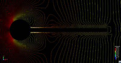
|
| Figure 24: Influence of stabilized fractional step iteration on pressure field - Note that the isobars are not perpendicular to the moving structure anymore |
The actual influence of this modification can be seen when having a look on the resulting pressure along a coupled interface where now a significant shift of the isobars should be observed indicating the differences between the boundary and the interior. For an illustration the improvement was applied to the well-known strongly coupled benchmark-problem in [40]. Figure 24 shows the isobars during the solution iteration in a time instance at the very beginning of the oscillation of the elastic beam. It clearly can be seen that the additional structure term was taken into account at the interface since the isobars are not orthogonal to the latter. In here we chose a parameter value of which corresponds to reduce the original proposed structural density at the boundary down to of its original value. Again it shall be emphasized that this modification only has an influence during the iteration in one time step. At convergence of the pressure state4 at the interface, 3.38 and hence the additional term in equation 3.42 vanishes which restores the orthogonality of the isobars again.
Finally it is worthwhile to mention that this additional structure term gets better and better in its accuracy the smaller the actual time step is. In the limit it even shows the correct structural behavior. That is the smaller the better this stabilization effect. Luckily the artificial added-mass effect behaves just reverse. So the smaller the worse the artificial added-mass effect. Effectively this means the method is all the more effective and accurate the worse the artificial mass effect is which is a very nice characteristic.
(1) Note that is a function of and generally nonlinear.
(2) See [39], page 41 for a detailed elaboration of the equations in a fractional step process.
(3) Effective mass means the the mass which responds with interia forces to a given movement of the fluid boundary
(4) Note that convergence at the interface might be checked for the displacements, the pressures or both together. In cases where only a convergence of the displacements is checked a negative influence of the stabilization technique can not be excluded since a convergence of displacements does not guarantee a convergent pressure state.In these cases hence the additional stabilization term may introduce accuracy errors or may even cause the simulation to fail.
4 Improving the computational efficiency
In FSI scenarios it is necessary to solve the whole coupled physical system of fluid field and structural field under suitable coupling conditions at the interface within one, typically iterative, simulation. Having the anyways computationally demanding single-field simulations, this generally increases the computational costs critically - depending on the chosen solution approach in some situations more and in others less. So strategies to improve the computational efficiency on any level play a crucial role. To this end, we want to present within this chapter several strategies that can be applied in different kind of situations .
In the first section we will thereby concentrate on parallelization techniques. In here different computer architectures will be analyzed briefly from a general point of view and in particular in terms of how they offer possibilities for improvements in the context of an FE-analysis. Furthermore different measures to allow for an evaluation of the quantitative benefit of a parallel environment are to be introduced. They are going to be used for efficiency analysis in subsequent chapters.
In the second section we will focus on a particular efficiency problem given for the embedded approach, i.e. the necessary spatial searches. In this context two different strategies will be introduced that were adopted and customized to face this problem as effective as possible. Since these strategies were adopted from a vast and living field of science, we will stick here only to the main ideas in the particular context of the embedded FSI analysis. All of the discussed strategies eventually were applied in the course of this monograph.
4.1 Parallelization techniques
Parallel computing is a technology that enables to divide larger tasks into multiple discrete subtasks according to the divide-and-conquer principle. These subtasks are executed simultaneously and therefore allow an efficient improvement of computational performance. As there is such a large demand for powerful resources and parallelization techniques in the field of simulations literature provides a vast offer of papers and books dealing with parallel computing. In the framework of this chapter we mainly refer to [41], [42] and [43]. Particularly, the book of Michael Quinn, [41], is highly recommended as it provides a basis for programming with OpenMP and MPI in C.
4.1.1 Potential and challenges of parallel computing
The technology of high performance computing provides an enormous potential which can be exploited in the field of Finite Element and FSI simulations. The most attractive arguments for dealing with parallel computing in the course of this monograph are summarized in the following overview:
- Reduction of computation time: The simulation can be computed in a fraction of the time needed by a sequential computation. By dividing the problem in N processes, the simulation can be computed up to 1/N times faster.
- Solve larger simulations: Larger simulations of a specific FSI problem e.g. caused by a much finer fluid mesh or a smaller time step can be computed in the same order of time. A computation which is N-times more expensive can be run within the same time.
- Concurrency: Several simulations can be executed simultaneously.
- Parallelization of FEM: The idea of the spatial discretization of a fluid or a structure into small elements allows to decompose the domain into pieces which are assigned to multiple processors. Due to the fact that the element-wise contributions are separately assembled into the global stiffness matrix, the finite element computations can be executed on each processor separately.
- Making use of the powerful Spanish Supercomputing Network (Red Española de Supercomputación)
Distributing the tremendous computational effort for a complex FSI simulation to multiple processors such that the computational efficiency improves, however, also brings some tricky challenges. The following list shows just the most significant challenges which we will face within this monograph:
- Larger implementation effort compared to sequential programs: In general, parallel code is much more complex than serial code. Multiple instructions are executed at the same time, but there might also be a data transfer between these instructions. Special functions are required to control the data transfer in order to avoid e.g. memory access conflicts. Also debugging is much more complicated.
- Load balancing: How to distribute the work between the processors? A perfect load balancing is reached, when all instructions executed by the processors are finished at the same time. The code is imbalanced if instructions need different times to finish their work and the processors are waiting for other processors to finish. This results in unused computing potential which decreases the efficiency of the parallel code.
- Dead locks: Several instructions are waiting for the other to finish but none of them is ever able to finish.
- Data transfer: When a process generates data which are processed by another one, they need to exchange data. This requires that the processes are executed in a certain order. Setting up the communication, synchronization and the order of transferring data is a difficult part of parallel computing.
- Race conditions: Processors are accessing the same memory at the same time resulting in a reading or writing conflict.
- Scalability of the problem: Describes the capability of the parallel code to handle larger amount of data by an increased number of processors. This is especially important to achieve in the framework of this work because large simulations for benchmarking will be used. The scalability is limited by the memory bandwidth in desktops equipped with multi-core processors [42].
- Overhead: The effort for managing the division of tasks into smaller packages, load balance between the processors, the communication, synchronization or also inclusion of external libraries requires a certain amount of time which is called overhead. The overhead always has to be compared to the time saving gained by the parallelization. When the overhead is larger than the time saving, the parallel simulation even gets slower than the sequential simulation.
- Efficiency of parallelization: Before parallelizing a code, one needs to think about the question: Is it worth to use parallelization? If the solution of a 3x3 matrix is supposed to be parallelized with many processors, the parallel computations will be even slower than the sequential computation.
A very fundamental question in parallel computing is how to organize the memory which every processor is accessing in order to solve the physical problem. The most basic architecture is the uniprocessor (figure 25: a single processor accesses the main memory via a bus which is also connected to the input-output system (I/O). In order to reduce the access time to the main memory, a cache is interposed between the processor and the memory. Frequently used data is copied to the cache from which the processor can read much faster than from the main memory.
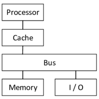
|
| Figure 25: Architecture of uniprocessors - A single processor accesses the main memory and the I/O systems via a bus. |
Thinking in terms of parallel computing, a natural way to realize a parallel computer architecture would be to add multiple of these processors to the same bus and give them access to the same memory. Systems which are based on this principle are called shared memory machines (SMM) (figure 26). Whenever any processor is invoking a change of data in the memory, these changes are also visible to the other processors.
A main drawback of SMMs is that the shared memory and the bus feature a limited bandwidth, which is divided among the multiple processors. An alternative architecture is provided by the so-called distributed memory machines (DMM) (figure 27). In these architectures each processor addresses its own memory which is not accessible by the others. Therefore each processors can exploit the full bandwidth to its own memory. Nevertheless, DMMs require an interconnection network (e.g. internet or LAN) which is managing the communication between the local memory of each processor. Supercomputers and clusters - which are accessed in the framework of this monograph - are based on the technology of grid computing which is in turn a form of distributed memory architecture.
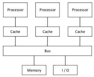
|
| Figure 26: Architecture of shared memory machines - All processors share the same memory. |
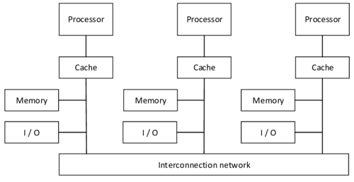
|
| Figure 27: Architecture of distributed memory machines - Every processor has its own local memory. |
SMMs and DMMs are conceptually different architectures and therefore entail intrinsic advantages and disadvantages. Both architectures will be used in the framework of this monograph. Therefore table 2 presents the main advantages and disadvantages of SMMs and DMMs. The main reason for dealing with SMMs in the framework of this monograph was the easy implementation and the good scalability on a desktop PC. The main reason for using DMM concepts was the potential of exploiting large scalability on a supercomputer.
| Shared Memory Machines | Distributed Memory Machines |
| All memory is stored in a global address space which can be accessed by any processor resulting in equal access time to the main memory. | If a processor needs to access data from the memory of another processor, messages have to be exchanged between the processors. This in turn causes additional overhead required for constructing, sending and receiving the message. Apart from this, the access time to the local memory is quite fast due to avoidance of interference with other processors. |
| Easy to implement compared to DMMs. This is also because the programmer can avoid partitioning of data. | Much more implementation effort because of managing load balancing or data transfer between the processors' local memory. Also debugging is very complex. |
| Memory bandwidth limits the number of processors to be used and therefore limits the scalability. | Memory bandwidth is much higher because each processor is only writing to and reading from its own local memory and can therefore use the full bandwidth of the memory. As a result, more processors can be used effectively, manifesting one of the main reasons for using DMMs. The scalability is much larger compared to SMMs and only limited by the interconnecting network. |
| Cache coherence: If a processor is modifying shared data which are stored in the cache memory of each processor, the changes need to be propagated to the cache of the other processors. | No problem of cache coherence because there are no processors which may overwrite data in the local memory of other processors. |
4.1.3 Quantitative performance evaluation
In order to be able to evaluate the improvements achieved by parallel computing and see how the performance of the parallel code is improved with an increasing number of processors, some basic quantitative measuring tools are needed. They are presented in the following. These are tools which will be applied in the later course of this monograph.
Execution time
The execution time of a program is the time between the start of the execution until the end of all computations. Supposed that not every part of the code is parallelized, there is the execution time for the serial code and the parallel code :
|
|
(4.1) |
whereas
|
|
(4.2) |
with the time required for the calculations and the time spent for all communication processes (waiting for messages, sending, receiving messages, ...).
Speedup
The speedup indicates the improvement of the parallel computation with n processors compared to the sequential computation using just one processor. The ratio of execution time with one processor and the execution time with n processors forms the speedup:
|
|
(4.3) |
Optimally, one can reach a speedup of n when using n processors, but typically in practice, the speedup is smaller than n due to e.g. overhead or not ideal load balancing.
Efficiency and scalability
The efficiency describes the relative improvement achieved by parallel computing and is therefore a convenient measure for the processor utilization. The efficiency is computed by normalizing the speedup with the number of processors as follows:
|
|
(4.4) |
The maximal achievable efficiency is 1. The larger the achieved efficiency, the larger the scalability, which is defined as the ability of a parallelized code to increase the number of processors efficiently when increasing the problem size of the simulation. But there is no generally accepted measure for scalability. Proposals are e.g. given in [44] and [45].
Amdahl's law
The impact of the sequential part on the achievable speedup as the number of processors increases is described by Amdahl's law. Let be the sequential part of a program code defined as . Then, the ideally achievable speedup can be calculated with the following formula:
|
|
(4.5) |
By increasing the number of processors, the speedup is converging as the next formula is demonstrating:
|
|
(4.6) |
As seen in the equation, the speedup is in fact bounded by the amount of sequential code. This implies that to achieve the largest possible speedup the sequential part of the code has to be kept as small as possible . In essence this law conveys the significant message for this monograph to parallelize as much as possible to get the best benefit from parallel computing.
4.1.4 Parallel computing with MPI
The commonly used standard application programming interface for managing the communication between processors in distributed memory systems is called MPI (message-passing interface). By sending messages containing a part of the local data of a processor via the interconnection network to another processor, this processor will get indirect access to these data - as already explained in section 4.1.2. The message-passing model is ideal for being used on supercomputers and clusters.
Using MPI to parallelize a program code can be very complex and time-consuming as it effects many parts of the program structure. In order to get a comprehensive understanding of how MPI is effectively used in Kratos and which implementation work has to be done for this project, let us consider the following flow chart in figure 28. It shows a general simulation process in Kratos, e.g. a CFD analysis.
The first significant step after initializing Kratos is the partitioning of the domain into smaller subdomains which will be distributed later to the processors and stored on the local memory of each processor. This partitioning should be done such that the communication between the subdomains at the interface is minimal and the number of simultaneous data transfers is maximal as additional time for communication increases the overhead. Geometrically this implies that the surfaces of the interfaces should be as small as possible. In Kratos, the external library METIS was chosen to do this partitioning as optimal as possible. In figure 29 such a partitioning of a meshed cube can be seen, on the left with 4 processors and on the right with 16 processors.
Each subdomain contains an interface mesh to each other subdomain with which it shares nodes. These information about interface nodes are required for the solution process as any movement of an interface node effects both subdomains it belongs to. In Kratos, these data are stored in the MPICommunicator class which sets up a communication plan based on these data. This in turn requires the creation of an additional data structure for the unstructured graphs. Furthermore, the class cares about the avoidance of dead locks.
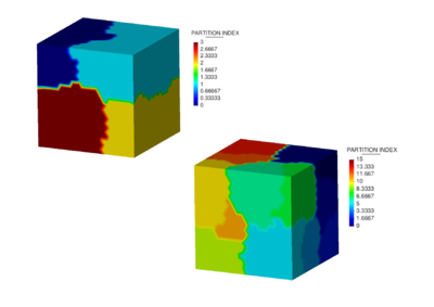
|
| Figure 29: Domain partitioning of a cube tetrahedra mesh - On the left hand side the cube is decomposed into 4 subdomains and on the right hand side into 16 subdomains. |
Subsequently, the subdomains are equally distributed to the processors. In each subdomain, the contribution of the local elements to the global stiffness matrix is computed. This setup of the global stiffness matrix in parallel is done by the external library Trilinos. Based on the stiffness matrix, the local equation systems are solved by each processor. The solution of each interface node needs to be updated afterwards as the solution variables are superposed at the interfaces. Finally, the results are written and visualized in one file.
The set of functions required for the parallelization of code in MPI is already available in Kratos, such that the Python script could be easily customized to work in parallel. Finally, the script can be called via the terminal with the following command:
|
4.1.5 Parallel computing with OpenMP
The application programming interface which is commonly used for shared memory programming is OpenMP (open multi-processing). The main reasons for using OpenMP are that it is easy and flexible to use for implementation and it supports the portability between different platforms, which is why it was also used in the framework of Kratos. OpenMP is based on parallelizing program code on the level of loops by dividing the loop into independent iterations which are executed in so-called threads - sequential executable code blocks of a process.
The principle of the task division to multiple threads is called multithreading and works as follows. Let's consider a computer with four processors, whereas each of them is responsible for one thread. After starting the program, a single thread - the master thread - is executed by processor 0, which is running the sequential parts of the entire program. Whenever there is a parallelized loop in the code, e.g. a parallel for-loop, the master thread creates additional threads which are assigned to the other processors (see figure 30. All these threads and the master thread are executing the partitioned work of the loop concurrently until the loop is finished. Then, the created threads are just deleted and the master thread continues with the sequential part until it encounters the next parallel section is following.
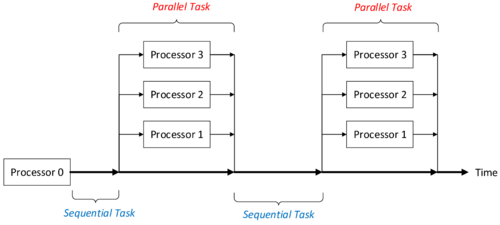
|
| Figure 30: Function principle of multithreading - One master-thread is responsible for executing the sequential tasks and for creating the threads in parallel sections. |
Multithreading is the key characteristic for OpenMP and basically the main difference to MPI. Whereas in OpenMP one thread is active from the beginning till the end of the program and additional threads are dynamically activated throughout the course of the program, in MPI all the created processes remain active from the beginning till the end of the executed program. This also enables incremental parallelization, which is a significant advantage of OpenMP compared to MPI. In essence, this means that the sequential code can be incrementally transformed into a parallel code giving the programmer the possibility to concentrate on parallelizing the most time-consuming blocks of the code without changing the code structure significantly. This is not possible in MPI [41].
As already indicated, OpenMP is mainly used for the speedup of loops. In the framework of this monograph we will concentrate on the parallelization of for-loops as it is quite easy to implement. Particularly, it will be applied to loop over all finite elements of a discretized domain. In Kratos, this is done by simply partitioning the model into N-1 elements, wheras N is the number of used threads and one thread has the functions as master thread. Within the for-loop the compiler distributes these partitions to the threads which are executed by the processors. The syntax of the corresponding key command is as follows:
|
This command indicates that the following loop is executed in parallel. It is important to realize that all the threads share the same database stored in the same memory, Therefore one needs to take into account race conditions during the implementation. This is especially the case when changing data stored on nodes, which belong to elements of different threads.
4.2 Spatial search
The techniques of parallel computing, as they were discussed above, offer a way to improve the computational efficiency in fluid-structure interaction analyses. In fact they are already widely spread in this context and generally not restricted to any specific solution procedure. In terms of the embedded approach, however, there is another important factor, that is influencing the computational efficiency and hence requires a dedicated solution beyond a pure parallelization.
In the embedded method we are letting meshes overlap without specifically define a common boundary. The actual coupling, however, requires an exchange of quantitative information along an interface, which therefore first has to be identified. As a consequence of the missing technical links between the meshes both the information exchange and the identification of the interface are somewhat depended on spatial search techniques, that are commonly not necessary in a body-fitted approach. Spatial searches, though, are computationally very demanding, which is why the choice of proper methods becomes particularly important. In the following we will briefly discuss the corresponding methods that were applied to this purpose throughout this work.
By construction the embedded approach contains two different steps for which a spatial search strategy has to be applied. That is:
- Given a structure node we have to find the fluid element in which it is contained (necessary for the mapping of quantities at the interface) and
- given a fluid element we have to find the embedded structure nodes (necessary when we want to check for intersections and hence identify the interface).
Both steps have in common, that basically either every structure node has to be checked against each fluid element or vice versa, which without any improvements ends up in a search algorithm of complexity . For highly refined meshes this quickly leads to an explosion of the computational costs, knowing that for instance the mapping of pressures or velocities has to be performed at every time step in each iteration. Luckily, however, a spatial search of this type poses a classical problem in computer science for which various techniques are available. Two powerful methods that were incorporated into the given embedded approach shall be introduced conceptually in the following. The aim is to provide a basic understanding plus the necessary key words for a possible literature research. Neither technical details will be elaborated nor any exhaustive comparison will be provided. Instead we are focusing in later chapters on their actual performance in the present practical application.
Besides of the fact that both of the above searching steps principally require to check every fluid element against each structure node, there is an important difference that is crucial for the choice of a proper spatial search method: In case where we want to identify intersections, we are searching for an entity in the domain of the structure, whereas in the other case we are searching for an entity in the domain of the fluid. Both domains are typically differing significantly in their shape. The fluid domain for example often is modeled as a convex hull over the structure, such as a block or a channel. The structure by contrast takes in general an arbitrary shape.
One method that is very well suited for regular distributions and superior with convex shapes is the spatial search based on bins. A bin is a data structure which basically divides the space into a number of regular cells as indicated in figure 31. Each cell of a bin knows about the entities it contains or it is intersecting with. So given a position in space we can ask for the corresponding cell and hence for the entities contained in this cell.
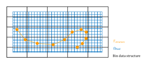
|
| Figure 31: Bin data structure - The picture shows the concept of a bin data structure applied to the situation of an embedded FSI scenario. Note that the situation equally holds for 3D. |
Generally it holds, the more regular the shape on which the bin is based, the more efficient the search. In fact if the shape is regular or convex, this method is superior compared to other techniques. Since the fluid domain often is regular in an embedded approach the method performs in particular efficient when applied to the fluid domain. Because of that the bin-search is the method of choice for case 1 in the enumeration above. Here the bin data structure is based on the overall fluid domain whereas each cell knows about its containing fluid elements, e.g. tetrahedra. So to search for the fluid element in which a given structure node lies we create the bin data structure once and then with each new search ask for the cell in which the given structure point lies. The cell in turn holds a list of possible candidates. All we have to do finally is to check whether the structure node lies within one element of this small subset of all fluid elements. By that the complexity of the search drops from to .
This is, however, only true for convex, regular shapes of the search space. In fact the computational effort quickly rises with more complex or non-convex shapes. In all the latter cases other alternatives, such as tree-based search methods, may perform better since they are taking into account the spatial distribution of the underlying data. This is why for case 2 of the enumeration above, an octree search was implemented.
In case 2 we had to find the embedded structure nodes of a given fluid element in order to be able to identify intersections and hence the common interface. To efficiently search for respective nodes, the structure is represented by an octree. More precisely, a given domain is divided into eight equal cubes, which are again partitioned into eight equal cells be it that a cell contains elements of the structure. This process is performed several times up to the desired level of refinement1. As a results the structural domain is decomposed by a tree-like data structure, i.e. an octree in 3D or a quadtree in 2D, respectively. The idea is conceptually illustrated for the 2D case in figure 32. The method applies accordingly in 3D.
The idea now is that the domain in which the octree was created not just contains the entire structure but also comprises the domain of the fluid. By that the single cells do not only know about embedded structure nodes, but it is moreover also possible to assign to each fluid element the set of cells of the octree which are intersecting with the corresponding fluid element. The respective cells are here obtained by applying the algorithm from Akenine-Möller [47]. Based on this linking, the effort for the identification of the intersections between the fluid and the structure elements can then be eased significantly for basically the same reason as already in the bin-search: Instead of checking every fluid element against each structure element we are for a given fluid element just checking a small subset of all the structure elements for intersections. This reduces again the complexity to an order of .
Different to the bin search, however, this method particularly performs well for arbitrary irregular shapes. Figure 33 shows in this context a large scale example from another application field. The advantage is obvious when noting that the octree leaves (cells at the lowest level of the octree) are closely concentrated along the boundary of the structure. Again transferred to our case case, this reduces the number of fluid elements that have to be checked for an intersection to only a few possible candidates.
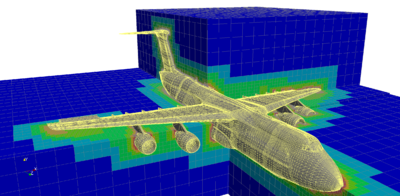 ] ]
|
| Figure 33: Octree mesh around a complex airplane model - The picture was taken from Zudrop in [48] |
This reduction of complexity for highly irregular shapes could also be achieved by tree-based structures other than the octree, for example by using a k-d tree instead, which in the latter case might even be more robust. But typically the octree is faster compared to comparable techniques. Moreover practical experiences throughout the developments in this monograph showed that it is sufficiently robust in case of the embedded method which is why it is justified here to use this more efficient method instead of a k-d tree for example.
At the end of this chapter it can be summarized: For the two essential spatial searches in an embedded approach, a bin-based search and an octree-based based search are applied. Both are designed to reduce the computational costs connected to the spatial search significantly. Nevertheless, the spatial search in an embedded approach can be considered as disadvantageous compared to a body-fitted approach where these searches are not needed for a coupling. Since on the other hand, however, the embedded method is not dependent on any mesh-regularization, the actual advantage or disadvantage in terms of the computational effort remains to be investigated.
(1) A detailed description of the specific algorithm that is applied here, also with regards to its computational aspects, can be found in [46]
5 Development & simulation environment
In the course of this chapter Kratos as an FEM-based multiphysics solver will be introduced in conjunction with EMPIRE (Technical University Munich, TUM), a coupling software that is able to carry out co-simulations with an arbitrary number of solvers. Both software packages together form the environment of the entire developments and simulations in the remainder of the present monograph. Thus in order to facilitate the understanding of the later discussed implementations plus also to provide a short reference for people from either development teams, the essential concepts of both software packages shall be introduced in the following.
To this end, the first part of this chapter focuses on Kratos and in particular on its main class structure as well as the principal work flow which arises from the FEM-specific implementations. Based on that it will be explained how the problem is formulated within the so called Model Parts and how Kratos approaches the solution of the latter by a distinct segmentation of the single solution steps. This is important since it affects the later implementations significantly. The explanations mainly follow the descriptions in [6,49]. A more user-oriented format of the principal workflow can be found in [39].
As a goal of this work, Kratos is to be applied together with other solvers in a co-simulation environment, in particular with Carat, the structural solver of the Chair of Structural Analysis at the Technical University Munich. This is where EMPIRE comes into play. EMPIRE is used as control and communication instance in this regards.
The second part of this chapter deals with an introduction to the basic concepts of EMPIRE. It starts with an outline of the principal layout of a respective co-simulation and afterwards concentrates on how different solvers can be connected and linked together to a co-simulation network. Here focus is set on the interface between EMPIRE and the connected solvers, i.e. the EMPIRE_API. The chapter then closes with a short description of different intern features which are necessary for a proper co-simulation, such as e.g. filter routines. Explanations in terms of EMPIRE mainly follow the descriptions in [50]. In there also two benchmark examples can be found.
5.1 Kratos
Due to the increasing demand for more and more realistic simulations of engineering problems the separate consideration of occurring physical phenomena (e.g. fluid mechanics, structural mechanics) is not sufficient any more. Rather more, it is necessary to account for the interaction between such fields leading to the coupling of physical quantities.
Those coupled fields result in partial differential equations which can be solved by means of the finite element method. Many conventional FEM codes are catered and optimized to the solution of physical problems including only one single field. The interaction of two or more fields therefore requires an external program managing the interface between the FEM codes, which at the same time lowers the flexibility towards other problems. This is, where Kratos as a unified software environment comes into play.
Kratos is an open-source software for solving multiphysical finite element problems. It is developed at CIMNE with the aim to provide a high level of data structure flexibility, modularity and reusability of the code. These advantages can be assured by a code written in the object-oriented language C++. C++ supports a generic programming which can provide a package of geometrical elements and algorithms that are widely decoupled from the specific physical problem. Therefore, new FE-codes can be easily added to the basic structure of Kratos. The object-oriented approach is particularly suitable for the implementation of finite element concepts. All these aforementioned design principles form the requirements for the efficient solution of multidisciplinary problems.
In Kratos, the objects in the framework of its object-oriented structure are constructed based on the general finite element approach. A very fundamental class structure can be found in figure 34 which at the same time represents the general work flow of a finite element analysis in Kratos. In the course of this chapter these concepts and the relation between these objects will be introduced and linked to the idea of a multidisciplinary framework based on FEM.
![Main class structure in Kratos - The figure gives an overview about the essential classes and their main objects in Kratos (adapted from [49]).](/wd/images/thumb/6/65/Draft_Samper_908356597-monograph-J01_ClassStructureKratos.png/500px-Draft_Samper_908356597-monograph-J01_ClassStructureKratos.png)
|
| Figure 34: Main class structure in Kratos - The figure gives an overview about the essential classes and their main objects in Kratos (adapted from [49]). |
In view of the modularity and flexibility of including new physical phenomena Kratos distinguishes between the kernel responsible for numerical computations and programming and the actual physics of the problem which is implemented in separate applications. This distinction is very important to mention because it allows to define new applications characterized by an own set of dofs, variables and elements whereas the underlying finite element methodology and solution algorithms are managed by the Kratos kernel. Applications such as fluid-structure interaction can also depend on other applications such as in this case e.g. the fluid dynamics application. The interface between these applications manages the communication and is also controlled by the Kratos kernel. These relations are illustrated in figure 35.
In order to ensure a time-effective development process and to provide a high level of flexibility in executing physical examples which access the application libraries, Python is used as scripting language. During this so-called end-user development the compiled Kratos libraries are imported as required and thus enables the direct access to the functions within these libraries without recompilation.
Referring again to figure 34, the kernel and the applications manage the library interface. An additional element within this main class - the input-output module - gives the user the opportunity to include his own concepts without touching the application itself.
All the applications have the finite element core in common which handles the solution process, discretization and the numerical description on element level. In order to understand the object-oriented implementation of the FE approach in Kratos, it is necessary to explain the most basic entities in Kratos in a bottom-up approach. A graphical summary is given in figure 36. Nodes, elements and conditions represent the basis for the finite element formulation as it is the core idea to divide the geometrical domain into simple geometries (e.g. triangles or tetrahedra) which can be treated by a set of fundamental algorithms. The very basic entities of such geometries are Nodes which are characterized by a unique ID, the spatial position and a list of dofs (e.g. fixed displacements in x-direction). The dof class is basically described by its variable, the state of freedom in terms of any Dirichlet boundary condition (fixed or free) and its actual value. The dofs together with all variables are collected in a database in two different containers: nodal data (non-historical data only storing the current value as e.g. the list of adjacent nodes) and solution step nodal data (historical data storing both the current value and values from previous time steps - mainly variables related to the time iteration).
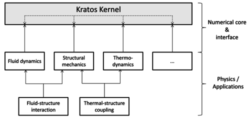
|
| Figure 35: Relationship between kernel and applications - Kratos separates the numerical core and FE description from the physical applications |
A collection of nodes leads to the geometrical definition of an element which itself is implemented in a separate class Geometry and also contains FEM-specific data as the shape functions or the Jacobian at the corresponding node. The Geometry class therefore constitutes the foundation for the definition of an Element which contains a large part of the physics of the FEM problem. Within an element, all the available information are collected to compute the elemental matrix on the LHS of the fundamental local linear system of equations as well as the RHS. These matrices and vectors are later assembled to the global system of equations. Contrary to this, conditions are faces of a finite element directly at the model boundary, which implies that they are used to impose boundary conditions to the system. Any intrinsic information of the elements as material properties of a structure are stored in the Properties class.
All these data are practically bundled within the Mesh class as a container storing the nodes, elements, conditions and properties constituting the region of interest in the domain to be simulated. Several meshes can again be collected to a Model Part which eventually represents the most important class in Kratos as it comprises all necessary information for carrying out a simulation. Therefore additional data as the process info specifying e.g. the current time step of the simulation are also stored as part of the model part. During a preprocessing the complete model part has to be created which then forms the basis for all relevant simulations.
After having defined the main components which completely describe a model in Kratos, the system of equations needs to be solved with a solver which can be chosen according to the requirements of the individual problem. The complexity of solving such huge systems of equations results in a variety of solvers which are at the same time executing a bunch of algorithms. In Kratos this is in general implemented by means of the Process class. The latter handles different tasks ranging from computing the normal of a triangular element to the search for adjacent elements of a node. An important derived class of Process is the Strategy class which is managing the solution steps of the FEM problem. For every problem the finite element algorithms can be uniquely separated into the following basic steps:
- Time iteration: requests the local contributions from each element (more precisely the stiffness matrix, damping matrix and mass matrix) to the global system matrix and the residual vector as well. These matrices and vectors are combined to form an effective matrix and effective residual vector by using a certain time iteration scheme.
- Build equation system: assembles the effective terms of each element to one global system matrix and a global residual vector provided by the time scheme at each iteration step.
- Solve equation system: having the linear system of equations, this step calls a linear solver to solve the system.
- Update database
- Check convergence (if required)
- Calculate output data (if required)
In Kratos, the time iteration (step 1) as well as the updating of the database (step 4) are combined to the Scheme object. Moreover, steps 2 and 3 are combined to one common object called BuilderAndSolver. These two objects form the main ingredients for every strategy which is implemented in Kratos. It is important to note that Kratos generally uses a monolithic solution approach when solving multi-field problems. That is that the BuilderAndSolver in this case sets up and solves a global system of equations which comprises the problem specific equations as well as respective coupling terms. A partitioned approach is not explicitly implemented.
Completing the discussion about the most important classes in Kratos according to figure 34, it also has to be mentioned the group of numerical tools. It contains some basic auxiliary means provided for the implementation of the FEM. Besides of Matrices and Vectors, there is an object to provide various Quadrature Methods, an object defining essential Linear Solvers e.g. exploiting the sparse global matrix characteristics typical for FEM. Data Containers and the aforementioned Geometry object are further advanced techniques in order to improve and extend the performance of the preexisting C++ libraries.
Having a bunch of classes in Kratos at hand, it is crucial to shortly go into the setup of a simulation. As mentioned before, the model part contains information about the geometry, the mesh and also the imposed initial and boundary conditions. At CIMNE, the preprocessing tool GiD is commonly used to define the full model part graphically, which is automatically transferred to a text file, the so-called .mdpa-file. Additionally, a Python file ProblemParameters.py containing the problem settings - such as the solver setup, the process information or the postprocessor configuration - is generated by the software. That file is read from the main Python script which coordinates the complete simulation process by loading all necessary libraries and physical data, defining the solver and additional process functions as well as managing the solution process. The main script is named either KratosOpenMP.py or KratosMPI.py depending on whether the program is parallelized with OpenMP or MPI. After finishing the simulation process, the results can be visualized with the postprocessing function of GiD.
5.2 EMPIRE
Solving coupled multi-field systems using a partitioned approach has the particular advantage that different existing and possibly well-tested solvers for the respective single-field correspondents can be reused as black boxes in a multiphysical analysis. This is not only advantageous from a user point of view but is also attractive since it allows to combine technical knowledge in cooperations across single institutions. A partitioned approach, however, requires information exchange among the single codes which has to be managed in a specific co-simulation environment.
At the Chair of Structural Analysis at the TUM such a modular partitioned solution approach is pursued in order to facilitate cooperations with acknowledged experts in the field of computational mechanics. One specific goal in this context is to be able to perform FSI simulations using Kratos as a fluid solver in combination with the in-house software Carat as a solver tailored to structural problems. To this end the Chair of Structural Analysis continuously develops its own open-source coupling software called EMPIRE (Enhanced Multiphysics Interface Research Engine).
Throughout its development EMPIRE is kept generic and thus allows the simulation of not just two but also several coupled fields. It is for example possible to investigate fluid-structure interactions while monitoring the physical quantities in a control circuit which in turn actively influences the interaction as it is often the case in practical applications. In fact EMPIRE is virtually unlimited in the number of couplings and thus allows n-code co-simulations.
Regarding its structure, EMPIRE principally consists of two components, the coupling code Emperor and the application programming interface (API) which is referred to as the EMPIRE_API in the following. The latter is a necessary interface for a proper communication with the different simulation codes whereas the first manages the entire communication. The general communication pattern in a co-simulation using EMPIRE is depicted in figure 37. Following the terminology in [50], each link represents a communication instance or a connection between solver and the Emperor. Each connection is used to exchange specific information such as the displacement or pressure field in a fluid-structure simulation. For the sake of consistency output and input are distinguished as it is done in the figure. The Emperor acts as a hub in this network hence the latter as a whole poses a common server-client model in which both bilateral and unilateral communication is possible as indicated in figure 37. It is important to note that the single clients, i.e. the simulation codes, indeed communicate with the Emperor but are running independently and do not have to know anything about each other. The advantages regarding modularity and flexibility are obvious.
![Co-simulation with EMPIRE - The figure shows the principal communication within a co-simulation controlled by EMPIRE. (Adapted from [50])](/wd/images/thumb/a/aa/Draft_Samper_908356597-monograph-D01_CoSimulation.png/400px-Draft_Samper_908356597-monograph-D01_CoSimulation.png)
|
| Figure 37: Co-simulation with EMPIRE - The figure shows the principal communication within a co-simulation controlled by EMPIRE. (Adapted from [50]) |
Since the simulation codes are generally independent and Emperor only manages the respective inputs, each client has to have an interface to EMPIRE, i.e. functions which for example allow to send field data in the expected format to EMPIRE. This interface has to be implemented in the single client codes, like Kratos, according to the given specifications in the EMPIRE_API. The latter is written in C++ but contains a linkage to C which enables it to be used by different compilers in these languages and furthermore by some dynamic libraries like Python. This facilitates the integration of communication routines in Kratos, since its user is intended to operate exclusively on Python level. Regarding the communication between Kratos and EMPIRE in particular the functions of the API which are listed in table 3 have to be imported in Kratos to establish an interface to the Emperor.
| Function | Description |
| connect | Establish connection to the server (Emperor). |
| getUserDefinedText | Get information from XML File. |
| sendMesh | Send mesh of the client at the coupling interface to the server. Receiving a respective mesh is not possible yet. Note that EMPIRE can work with multiple meshes but not multiple partitions, so possible pieces should be assembled into one mesh before being sent. |
| sendDataField | Send field data to the server (e.g. displacement field on structural solver side). Field data in this context is defined on a mesh, this function thus implies data mapping. |
| recvDataField | Receive field data from the server (e.g. displacement field on fluid solver side). Field data in this context is defined on a mesh, this function thus implies data mapping. |
| sendSignal_double | Send a simple data array which is not necessarily linked to a mesh. |
| recvConvergenceSignal | Request convergence signal from server. |
| disconnect | Close connection to the server. |
Multiphysical problems usually involve a high number of degrees of freedom. In order to account for the respective computational effort, EMPIRE can also run in parallel. In that regards it is important to note, that EMPIRE is partially parallelized using OpenMP. Furthermore it uses MPI for the connection of the single solvers as well as for the send- and receive-routines. It, however, doesn't do any domain decomposition or partitioning. This significantly restricts parallelization possibilities when using it together with Kratos which allows to partition the physical domain by making use of MPI.
 ] ]
|
| Figure 38: Filters in EMPIRE - Various filters can be applied and linked to modify data along a connection. [50] |
Apart from a parallelized run and the pure information exchange alongside a connection it might also be necessary to modify sent or received data. This is for example the case when connected clients are using non-matching grids for their simulations. Here a proper mapping has to be applied which is transforming the field information at interfaces from one grid to the other. Various kinds of modifications can be done by using respective operators which in the following, according to Wang et al. [50], are called filters. Filters can be applied both as single operators and as part of a filter network. Figure 38 illustrates this concept. A list with the implemented filters, that also were used in the scope of this work, is given in table 4.
| Filter | Description |
| Mapping filter | In a partitioned multiphysical simulation each single-field solver usually has a different discretization at the respective interfaces. This requires data mapping between two non-matching grids. Different mapping methods are implemented in EMPIRE to this end. We will use the Mortar Method in the following. |
| Extrapolation filter | An extrapolation filter is necessary when data at coupled interfaces has to be predicted in each new time step. |
| Relaxation filter | Relaxation can be used in iterative schemes to stabilize the simulation. |
All connections and filters have to be defined in a single XML-file which Emperor reads as input. Furthermore the XML-file bundles information about the single clients and contains settings with regard to the coupling algorithm and the iteration sequences. By that it is possible to realize different coupling strategies, both explicit and implicit. EMPIRE finally performs the simulation according to the settings in the XML-file. After having developed a communication interface, also Kratos can be invoked in this file making it possible to carry out partitioned FSI simulations using Kratos and Carat together in a co-simulation environment.
6 Kratos' interface to EMPIRE
In order to allow partitioned FSI-simulations using Carat and Kratos together in a co-simulation controlled by EMPIRE, an interface had to be created in Kratos that is able to establish a connection to the EMPIRE_API. As additional requirement, the interface should be designed such that it is not just able to be used within an ALE framework but also ready to be used within the framework of an embedded approach. The implementation and verification of such an interface is topic of this chapter.
In the first part the structure of the interface will be described following its basic classes and their mutual relations which will be summarized in a UML class diagram. It is shown, that the interface is ready to be used in a partitioned FSI-analysis using both an ALE and an embedded approach. In this context still present limitations will be explained. Apart from these limitations for each solution approach a generic process flow can be derived. Since the partitioned analyses in the course of this monograph are all customization of this generic processes, both of the latter will be elaborated in more detail by means of two graphical overviews. A short summary of the arising possibilities will then be given at the end of the first section.
Knowing about the implementation details the functionality of the interface will be verified in the second part. In particular a correct sending of the data, a functioning coupling and mapping as well as a correct overall communication will be shown by means of two distinct examples, i.e. a simple cube with imposed movement of the ground plate and an FSI-simulation of a beam in a channel flow. The results will finally prove a correct implementation which in turn was a prerequisite the later simulations.
6.1 Interface structure
In order to allow for co-simulations using Kratos and Carat together in one simulation by connecting it via EMPIRE it is necessary to set up an interface between the latter and Kratos. As already described in 5.2 EMPIRE already includes an API to which Kratos can be interfaced. A respective connection, however, requires additional implementations on side of Kratos which for a proper simulation have to be designed such that they comply with specifications of both software packages. How this implementation was organized and realized as well as how it is used in an FSI simulation is described in the following.
Crucial requirement in terms of the interface was a modular and flexible applicability in Kratos. That meant that at first a whole new application covering all relevant functionalities had to be created and embedded in the given structure. This new application, internally called "EmpireApplication", allows a usage in the same way as all the other applications in Kratos and thus offers a wide range of possible co-simulation scenarios. Figure 39 depicts its general structure.
In a second step the EMPIRE libraries had to be linked to the Kratos environment such that its functions can be invoked in that. EMPIRE is relying on its own libraries. Within one of them, all the functions of the EMPIRE_API, they are already described in 3, are defined. This library had to be linked to Kratos. In favor of compatibility a pre-compiled version of it was used. This eventually enables to link it dynamically in Kratos' Python scripts as needed in single simulations. Within the interface, the dynamically linked EMPIRE libraries resemble in a single object called ``libempire_api" (see figure 39).
Besides of the compilation also the different programming languages had to be considered. Since the EMPIRE_API is accessible via C-functions but Kratos in contrast uses Python for the setup and C++ for the run of a simulation, a further implementation requirement was a common format to exchange data from either programming language. In this case C-Arrays were used since they are principally processable by all these languages.
Due to the fact that both Python and C++ was used in Kratos, the advantages of both languages were to be exploited. That is why all iterative and computationally expensive routines were written in C++ while all the other serial tasks like input and output operations are directly accessible and modifiable within Python and hence do not need any recompilation. The outsourcing of the different routines required a careful conversion of the different data formats but eventually allowed an optimized performance.
After having created the general environment for the interface, the EMPIRE_API's functions according to table 3 had to be wrapped into that. The actual interface was thereby designed such that, depending on which framework one is choosing (ALE or embedded), the user has access to different features which are each based on the aforementioned API functions but customized to the specific problem. As a consequence two main Python classes appear in the application: "empire_wrapper_ale" and ``empire_wrapper_embedded. In both cases the interface can be integrated in a Kratos simulation by just creating a single object of either of these classes at run-time. The object then wraps the functions of the EMPIRE_API in the correct format and is consequently referred to as a wrapper in the following.
As already indicated before, some processes of the wrapper are outsourced to C++ as can be seen from figure 39.This obviously implies a connection of the two separate programming environments via an established Python-C++ exchange format. Through this connection the outsourced functions are contained in the C++ class "ale_wrapper_process" which hence covers all program parts that require an iterative or computationally demanding algorithmic such as reading or extracting information from the entire coupled system12. It is also used to extract the common physical interface for an ALE-approach or the embedded structure boundary in an embedded approach. In both cases information about the interface are stored as an extra attribute, which here is called ``interface_model_part. This facilitates the handling of the wrapper in Kratos significantly.
The C++ functions are just used by the wrapper objects of the two higher lever Python classes and hence do not have to be invoked in any position of the simulation. The latter wrapper objects are the one entities which are needed to set up the communication with EMPIRE. Therein included functions are posing the actual interface and will thus directly be invoked by the Kratos user who intends to set up an FSI-simulation for example. Typical functions here are the sending and receiving of field-information such as displacements or pressures. Most of the functions are simple customized versions of the already explained EMPIRE_API functions from table 3. Note, however, that additional features were included in order to enable:
- a co-simulation using several Kratos clients at once or even solely Kratos throughout the entire analysis with EMPIRE (highlighted in red).
- an exchange of mesh information which is is necessary when using an embedded approach(highlighted in orange).
By using all the these functions Kratos can be used together with EMPIRE to run n-coupling co-simulations without any great effort and for both an ALE and embedded analysis. Before, this was not possible. In consequence Kratos can be combined with further analysis approaches beyond the finite element method such as e.g. approaches from control theory. This not only follows the Kratos' philosophy regarding multiphysics but primarily offers various new applications.
There are, however, still limitations. Despite the implemented interface allowing already a co-simulation with both solution procedures, embedded and ALE, there is still a principal limitation, which is imposed by EMPIRE itself. The limitation here arises due to the fact that EMPIRE is not yet designed for embedded approaches and therefore indeed receives meshes from the client, through the function call “sendMesh”, but in turn cannot send mesh information to the single clients, which would require a function call like “receiveMesh” on client side. In an embedded approach, however, the fluid solver has to know the configuration of the current structure mesh in order to be able to identify the actual interface. Principally this can be achieved by receiving the structural mesh either in each time step or by receiving it once in the very beginning of the simulation and subsequently update it with the known displacement field at each instance.
Both of these options are however not yet possible with EMPIRE and still a matter of future project work. Nevertheless, in order to be able to carry out first partitioned analysis in an embedded framework using the features of EMPIRE, the interface contains a preliminary “receiveInterfaceMesh”- and a corresponding “sendInterfaceMesh”-function. These functions allow to exchange mesh information, i.e. node IDs, node coordinates, element IDs and connectivities, separately in the beginning of the co-simulation using the in EMPIRE given options of sending and receiving signals. When doing so, the wrapper automatically assembles the single information to a mesh of the fluid-structure interface in Kratos by using the function “CreateEmbeddedInterfacePart” and stores it as one of its attributes34. Even though this procedure was used within the scope of this work, in order to be able to investigate the capabilities of the embedded method in a partitioned approach, it has to be prospectively exchanged by a respective functionality in EMPIRE.
Having now all features at hand to carry out a partitioned FSI-analysis using Kratos via EMPIRE, two generic processes can be identified for the case of an ALE and an embedded procedure. In this context we are concentrating on the configuration where exclusively two Kratos solvers, one for the CSM and one for the CFD, are coupled. Each process flow and corresponding communication pattern can hence be outlined as done in figure 40 and 41. Partitioned analyses in the remainder of this monograph all follow these processes.
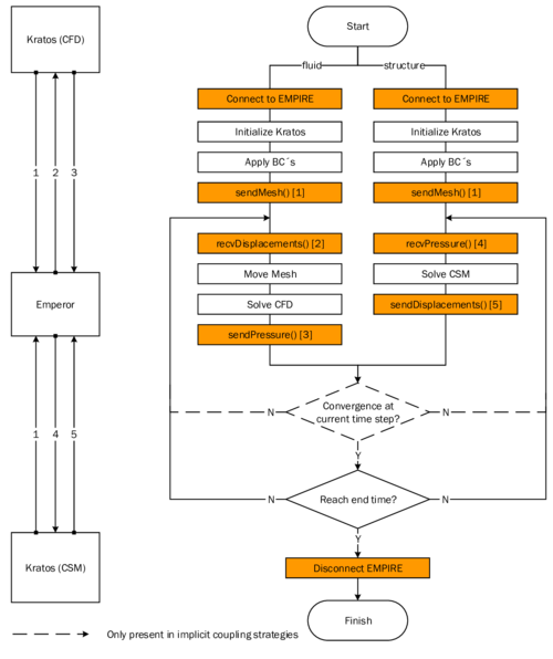
|
| Figure 40: Co-Simulation of an FSI problem in an ALE framework using Kratos and EMPIRE - The right chart shows the general process flow as an extension of the generic one from figure 3 by the above described newly implemented features of the EMPIRE interface (orange). The communication between the two different solvers is hence managed by EMPIRE (left). |
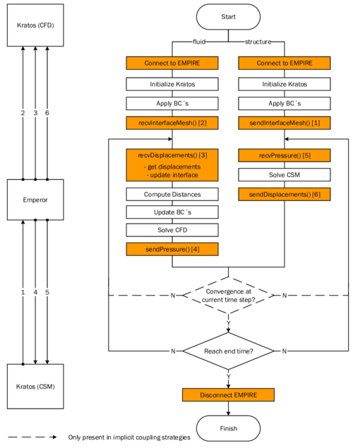
|
| Figure 41: Co-Simulation of an FSI problem in an embedded framework using Kratos and EMPIRE - The right chart shows the general process flow as an extension of the generic one from 4 by the above described newly implemented features of the EMPIRE interface (orange). The communication between the two different solvers is again managed by EMPIRE (left). Based on the latter, field data is mapped at the interface according to the embedded approach. |
From figure 40 and 41 it can be seen that a partitioned FSI-simulation using Kratos and EMPIRE only requires to invoke a few additional functions from the main Python classes in 39 either before the time evolution starts, during or after it. So the general structure of a Kratos simulation is preserved which facilitates is application significantly. Steps beyond the direct communication such as the mapping between to possibly non-matching grids are handled by EMPIRE internally and do not have to be specifically defined in Kratos.
Note that, as already mentioned in chapter 5.2, EMPIRE does not allow domain partitioning and hence a respective global parallel solution approach. This means that each single branch in the figures 40 and 41 indeed can use internally parallelization techniques, but the global solution process needs to be kept sequentially.
Note also that the wrapper offers the option to send and receive both pressure values and forces. Typically pressure values are sent since they are independent of the discretization unlike reaction forces that vary with changing degree of refinement as indicated in figure 42.The latter fact leads to difficulties when mapping between non-matching meshes and might result in a violation of equilibrium conditions. EMPIRE can, however, map consistently in both situations using the Mortar method.
At his point it can be summarized: The implemented interface covers all features to connect Kratos to EMPIRE while sticking to the specifications given by the EMPIRE_API. It manages both the communication between the different software packages and hence the different programming languages as well as the internal data management in Kratos. The structure of the wrapper is thereby chosen such that it allows an easy and flexible connection of one or even more instances of Kratos to EMPIRE. This enables various new scenarios of Co-Simulations in which Kratos can be used. Furthermore, preliminary functions allow a partitioned FSI-anlysis using Kratos together with EMPIRE in not just an ALE but also an embedded solution approach. Figure 40 and figure 41 outlined in this context the general process flows where exclusively Kratos-clients are present. This generic processes can be adjusted to realize different coupling strategies5. Furthermore, due to the fact that the clients are independent, it is just a simple step to replace the structural solver of Kratos with the one from Carat. That is that Carat and Kratos can now also be used together in a Co-Simulation environment. What remains to be done is a verification of the interface´s functionality. This is going to be topic of the following chapter.
(1) From an implementation point of view these program parts are included in Kratos as independent processes, which is why the respective class is derived from the parent class “Process” of the Kratos kernel
(2) Remember: All model information are contained in the Kratos object “model part”. That is why the model part appears as an attribute in both classes.
(3) The respective functions are highlighted in orange within the above depicted class structure.
(4) Note that this procedure does not require both clients to be Kratos, also Carat can be used assuming that it sends the same information in the same sequence. In this case, the customized “sendMesh” function would have to be adopted in Carat which is a straightforward task.
(5) By adjusting the input XML of EMPIRE
6.2 Verification
Having implemented the interface between Kratos and EMPIRE we can think about models on the basis of which it is possible to verify that the implemented interface conforms to the defined specifications and works correctly. This chapter is dedicated to proof this using a few simple examples. Here we are concentrating on the most important features of the interface. This is enough, though, to guarantee an error-less communication between Kratos clients and EMPIRE.
The testing will be organized as follows:
- The connection and data transfer is to be tested and verified by using a simple dummy FSI-configuration where a structural movement is manually imposed and transmitted to the fluid domain.
- Assuming a correct data transfer a correct mapping will then be tested by means of a beam placed in a channel flow.
- Having tested the essential sequential steps in the communication, a correct coupling of them within the full implicit FSI-analysis of the example from 2. will be tested. A subsequent physical interpretation of the results shall moreover proof a correct overall communication.
- Finally it is to be shown that for the case of an embedded approach, mesh information can be exchanged via EMPIRE as required.
Case 1-4 will be done using the ALE formulation and hence the respective ALE wrapper-functions. Without proofing it explicitly the results will also be valid for the wrapper-functions in terms of the embedded method.
6.2.1 Verification of a correct data transfer
As indicated above, first the connection of Kratos to EMPIRE and the correct data transfer is to be tested. Therefore the model shown in figure 43 was used since it provides a simple geometric setup allowing an easy tracking of the quantities of interest. The model is a two-dimensional rigid square plate placed at the bottom of a cube-shaped fluid domain. The idea is now to manually impose a movement of the plate in positive y-direction, send this movement via EMPIRE to the fluid solver and see what the fluid receives and how it reacts to this. The simulation is thereby such that with every time increment of the plate is moved by a displacement increment of :
|
|
(6.1) |
where
|
|
(6.2) |
The plate starts with the the movement at the very bottom of the fluid cube and has an identical cross-section such that the fluid is not able to flow across the edges of the plate. Due to incompressibility this requires a zero pressure at the opposite face enabling here a mass flux out of the cube. Obviously one can expect in total a “squeezing” of the fluid domain which finally can be measured. Even though this test scenario is clearly not an FSI-analysis, since it is only a unilateral coupling, it already includes the communication pattern of a such which is why the results of this test also hold for the fully coupled pendant. The communication pattern and the process flow of this test are depicted in figure 44. Note that here an explicit coupling scheme was chosen in which no relaxation filter is present. This was done since we are only interested in the pure data transfer. A manipulation due to a relaxation factor was to be excluded.
To investigate the movement of the fluid cube the displacements of an arbitrary node at the bottom of the cube was recorded along the simulation process. This has to correspond to the imposed movement of the structure if the communication is done correctly. In fact as shown in table 5 this can be observed. Figure 45 shows the respective results for the fluid cube after a simulation time of . Since the results coincide the data transfer can be considered to be verified.
| 0.0 | 0.002 | 0.004 | 0.006 | 0.008 | 0.010 | |
| 0.0 | 0.02 | 0.04 | 0.06 | 0.08 | 0.10 | |
| 0.0 | 0.02 | 0.04 | 0.06 | 0.08 | 0.10 |
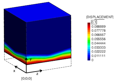
|
| Figure 45: Fluid domain with imposed plate movement after a co-simulation with EMPIRE - The picture shows the results of the partitioned simulation for a simulation time of . A significant movement of the fluid domain due to the imposed movement of the bottom plate can be observed. In fact the final displacement corresponds to the one that was expected after according to equation (6.2). |
6.2.2 Verification of a correct data mapping
As seen in the previous chapter, already a simple data transfer requires a data mapping as soon as non-matching grids are present. In particular the displacement and pressure field has to be mapped along the interface of the two domains in an FSI scenario. Using an embedded approach there is obviously no common mesh interface and the mapping is already included in the algorithmic of the method. In a partitioned ALE-formulation, however, a correct mapping has to be taken into account as a separate step. In this context Empire is using a Mortar Method to map between non-matching grids. The latter step in a setup where two Kratos solvers are connected to EMPIRE is to be verified qualitatively in the following.
Testing scenario is going to be a cantilever beam placed inside a channel flow. At the wet interface fluid and structure are each discretized differently in order to have a non-matching grid. This will require a corresponding data mapping between the domains. The respective model details can be found in figure 46. Furthermore the different interface meshes each of the fluid and the structure are shown in figure 47. From a physical point of view the complete setup is posing a flow-induced deflection problem, i.e. a classical FSI problem. For this we know the physical behavior, as will be detailed in the subsequent section, which is why it was taken also for verification purposes in the remainder of this chapter.
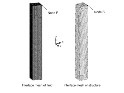
|
| Figure 47: Non-matching interface meshes - The picture shows the different meshes for the wet interface in scenario 46 |
Even though this problem is principally a fully coupled problem, we are in this section only interested in how the data is mapped at the interface. To this end we were running a unilateral coupled analysis of this model, which is similar to the one described in figure 44. Here we let the fluid flow fully develop and afterwards map at each time step the given pressure field at the interface on fluid side to the structure which in turn simulates the resulting deformation. Since we are only interested in the mapping there is no coupling of the resulting displacements back to the fluid which means that we are not resolving the entire fluid-structure interaction. The latter is going to be investigated in the following chapter.
Having simulated this test case one can compare the pressure field at the interface at each time step on structure side and on fluid side. A correct mapping requires them to differ only according to the limitations of the underlying mapping algorithm, i.e. for this case where we are using a Mortar mapping method with rather fine interface meshes, the pressure field on both sides should almost coincide. In fact as can be qualitatively seen from figure 48 they coincide. Since this is a generic process step for all FSI-simulations in this context, one can consider the mapping in connection with the above described data transfer using the Kratos-EMPIRE interface to be verified.
6.2.3 Verification of a correct coupling in a complete FSI
Having investigated the data transfer and mapping it is now to be tested and verified whether the complete coupling between the different Kratos solvers via EMPIRE works correctly. To this end we are using the scenario from figure 46. As opposed to the previous section, however, we will now apply a complete bilateral coupling of fluid and structure, i.e. we are simulating the complete FSI. Figure 49 details the corresponding process.
The aforementioned example is particularly useful for the verification of the coupling since we know the physics of this problem which is a flow-induced deflection (bending) of the cantilever beam. If the coupling of the different domains using Kratos and EMPIRE in a process as depicted in figure 49 works correctly, this physical behavior has to be recovered by the analysis. In the following this is going to be tested in two steps:
- check convergence in each time step,
- compare final results and double check physical significance.
Checking convergence is straightforward. Here we are looking at the step where the displacement field is transferred from the structure to the fluid (step 3 in figure 49). Since we are using an implicit scheme with Aitken method, we can test if the coupling formally is successful by checking in each time step whether the received displacement values on fluid side iteratively converge to the sent ones on structure side. To this end the displacement value for a specific node on the structure was compared to the value of the corresponding node of the fluid. Both nodes are highlighted in figure 47.
Table 6 summarizes the results from the analysis for the time step . As can be seen, convergence1 is achieved after steps. From this one can conclude to a working coupling between the two domains when using the Kratos-EMPIRE interface.
With the interface functions in terms of coupling, mapping and data transfer being verified it remains to test how all the single steps resemble to an overall FSI-analysis. To this end the beam was simulated in the complete FSI context. Intentionally the corresponding model parameters and boundary conditions from figure 46 were chosen to be such that a simple deflection of the beam without any flutter phenomena has to be expected. Note in this context the relevant Reynolds number of
|
|
(6.3) |
| Time step n = 30 | ||
| Structure (Node S) | Fluid (Node F) | Aitken factor |
| 0,013929187 | 0,013459557 | - |
| 0,013929706 | 0,013464254 | 0.01 |
| 0,013928829 | 0,013987717 | 1,12454 |
| 0,013928464 | 0,013928965 | 0,998332 |
| 0,013928250 | 0,013928499 | 1,00624 |
Despite the comparatively low Reynolds number we neglect the viscous influence of the fluid onto the structure and just use the pressure field as driving force for the structural movement. That is we simply need to transfer the scalar pressure field between the domains instead of the more difficult directional traction forces.
To investigate the deflection of the beam we again use the node indicated in figure 47 and measure its X-displacements as time evolves. The results are recorded in diagram 50. As can be seen qualitatively, the analysis gives exactly what we physically expected to get, i.e. a deflection of the beam in flow direction. Furthermore note that after a while the tip deflection gets non-linear in time which is also what we expect from the bending beam if the deformation becomes large. Figure 51 illustrates the results at the whole setup.
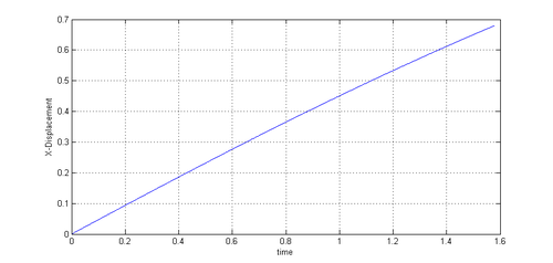
|
| Figure 50: X-deflection of a beam in a channel flow - The diagram shows clearly the expectable deflection in X-direction. Note the slight non-linearity as time evolves. |
Even though we are not evaluating the results quantitatively, we nevertheless observe that the physical behavior of the model is captured. From a qualitative perspective this clearly indicates a robust and working partitioned analysis. Since in this case the latter was carried out using the newly implemented Kratos-EMPIRE interface we can and have to consider its functionality as verified.
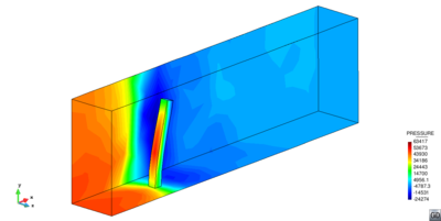
|
| Figure 51: Pressure distribution in the channel flow with elastic beam - The figure shows the results for the flow-induced bending of the beam at |
(1) Taking into account a tolerance of
6.2.4 Verification of a correct exchange of mesh information
As explained in section 6.1, a partitioned analysis using Kratos in connection with EMPIRE requires an exchange of mesh information at the wet interface of the structure. That includes the extraction and sending of the mesh on structure side as well as the receiving of the corresponding mesh data on fluid side. The newly implemented Kratos-EMPIRE interface allows this exchange of mesh information at an arbitrary instance of the simulation with the two specific wrapper functions, “sendMesh”- and “recvMesh”.
Their functionality can simply be verified by applying them to the problem of the beam above. To this end we are omitting the computation of the entire FSI but just concentrate on the exchange of the respective mesh information. That is, we extract1 and send the mesh of the wet part of the structure to EMPIRE using the customized “sendMesh”-function and ask EMPIRE subsequently for it by means of the new “recvMesh”-function. As a result the fluid solver is expected to own a copy of this mesh of the wet interface which eventually allows to apply the embedded algorithmic to it in order to identify the embedded boundary within the fluid domain.
Looking at the results that we get when actually applying these functions to the beam, a correct exchange can in fact be observed. The results are depicted in figure 52, where on the left the original solid beam mesh is shown and on the right the extracted and sent interface mesh. As expected the "sendMesh"-function extracted the wet interface of the solid beam, sent it to EMPIRE and the latter passed it to the fluid solver who asked for it via the “recvMesh”-function. It is obvious that it was sent correctly. With this also the exchange of the mesh-information between different Kratos solvers connected through EMPIRE is verified, i.e. possible.
(1) Assuming the interface is tagged as a such in some way, e.g. via a global Variable ``IS_INTERFACE"
7 Interface treatment in FSI problems
Every embedded method requires a proper tracking of the embedded domain and in particular the corresponding interface. Within the present chapter we will first discuss a collection of strategies which allows to represent and track arbitrary structures within an embedded domain. Then we will test its approximation error and influence on the overall solution with a few small- and large-scale examples. The corresponding tests and investigations are carried out at either generic or single-field CFD problems. The results are basis for the FSI simulations in the follow-up chapters.
7.1 Geometric description of the FSI interface
Within an FSI simulation based on an embedded approach it is required to provide a representation of the shape of the structure to the fluid solver. An efficient approach to handle this is the level set method based on distance functions which was already discussed in 2.2.4.1. Therefore a set of distance values for each element has to be computed as indicated in figure 6. Due to the fact that this approach is by definition just capable of describing one plane in each element, structures with many geometrical details can not be represented properly. In the following we will step-wisely develop an algorithm to treat structural surfaces of arbitrary complexity which can be categorized according to table 7. For each listed group representing a structural characteristic, the main challenges with regard to the interface treatment are emphasized.
7.1.1 Geometric approximation of plane structure surfaces
In the course of this chapter all the ingredients for an appropriate representation of a planar structure will be explained. Its starts with a mathematical description of the implemented algorithmic. After having a basic set of functions at hand, simple test cases will be discussed. As a representative test case we choose a rectangular plate. Furthermore a cube, which consists of six plates enclosing a volume, is tested in order to extend the validation to the general 3D case. The plate and the cube are significant benchmarks which are used for many validation examples in the later course of this monograph. The aim of this chapter is to describe the planar surfaces of these test cases properly by means of the discrete distance function.
In the framework of this monograph, the fluid volume is discretized by a three-dimensional mesh of tetrahedra, whereas the embedded mesh, discretizing the structure, is commonly represented by means of mesh of triangles. On the level of implementation, four basic tasks have to be performed, illustrated in figure 4 in the introduction. After the distances have been calculated they are assigned to the fluid element which in the following is marked as split using the flag SPLIT_ELEMENT.
Because we are generally able to describe with these distance values a plane exactly, also the algorithm for computing the distances, i.e. the distance function, needs to be able to represent a plane exactly. This first chapter explains the implementation of such a distance function. The plane as an infinitely thin structure and the cube as a volumetric structure with plane surfaces serve as examples for verifying the performance of the developed code.
7.1.1.1 Spatial search to identify intersections
As we are interested in the interface between fluid and structure it is necessary to look for all fluid elements which are cut by structure elements along the interface to the fluid. As we do not have any information about the spatial relationship between the fluid elements and the structure elements, a spatial search is necessary to reveal the intersecting structure elements. This procedure is visually explained in figure 53.
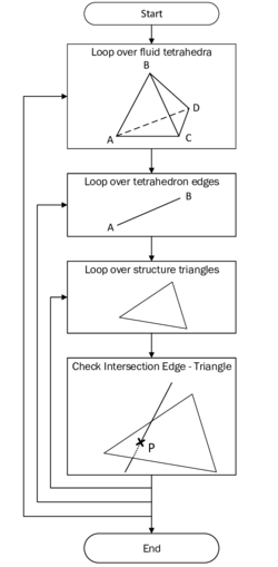
|
| Figure 53: Flow chart for spatial search - This flow chart shows the procedure for finding the intersections of fluid and structure elements. |
First of all, there is a loop over each fluid element. Due to the fact that there is no general algorithm to identify the intersection pattern of a tetrahedron with a triangle, the algorithm is reduced to an intersection algorithm of an edge of the tetrahedron with the structure triangle. This results in a loop over all six tetrahedron edges and for each edge again in a loop over all structure elements.
Identifying an intersection of an edge with a triangle is a basic procedure. We use therefore the algorithm proposed by Möller [51]. This code is effectively checking the existence of an intersection between a ray and a triangle. Having found such an intersection node, however, it is with this method still not clear whether this point is lying on the edge between the points and or somewhere else along the ray (see figure 54).

|
| Figure 54: Ray-triangle intersection - An edge with points and positioned on a ray is intersecting a triangle at the point P. |
To this end, the following geometrical consideration needs to be conducted:
|
|
(7.1) |
This basically implies that the connecting line of an edge point with the intersection point can not be longer than the edge itself. If this was the case, the intersection point P would not be an element of the edge .
After doing this procedure for all six tetrahedron edges of an element, each intersection node is put into a container which is set up for each element. This allows us to keep track of all intersection nodes. Let , , ... be the intersection nodes and be the set of all intersection nodes, then . Then, the cardinality of the set describes the number of intersection nodes for an element and characterizes the intersection pattern which is utilized in the following.
7.1.1.2 Computation of structure-approximated plane
Obviously, in the case there is no intersection between the fluid and the structure element, i.e. , no distances are computed, such that the fluid element keeps the initially set distance value of .
For each fluid element which is cut by the planar structure surface, we can have different intersection patterns comprising up to four intersection nodes. The intersection cases are listed in the following overview:
- : Triangle cutting one corner point of the tetrahedron (figure 55a).
- : Triangle cutting one tetrahedron edge whereas the two corner points of the tetrahedron are regarded as intersection points (figure 55b).
- : Triangle cutting three edges of the tetrahedron (figure 55c).
- : Triangle cutting four edges of the tetrahedron (figure 55d).
Due to the fact that we consider a planar surface, all of the found intersection points are lying coplanar within this surface. This will not be possible anymore for surfaces which are slightly curved. As a plane is described by a point lying in the plane and the normal of the plane, we can locally describe the plane for each fluid element by a single intersection node defined by its position vector and the normal vector which is predetermined by the orientation of the structural surface. Then, any arbitrary point which fulfills the subsequent equation is also lying in that plane:
|
|
(7.2) |
This equation basically expresses that any coplanar vector is perpendicular to the normal vector of the plane. Assuming a intersection pattern with three intersection nodes, this equation is fulfilled also by the coplanar points and as shown in figure 56.
The normal vector is simply the normal of the structural triangle which points into the same direction everywhere on the planar surface. By this we have all information at hand to compute the distance of the fluid nodes to the structure plane.
7.1.1.3 Computation of signed distances to the plane
The shortest distance between any of the four tetrahedron nodes, let us assume e.g. with the position vector , and the structure-approximated plane can be computed by means of the following equation:
|
|
(7.3) |
The notations refer to figure 57. The presented equation can be geometrically understood as the length of the projected connection vector onto the normalized normal vector. The point is one of the found intersection points, i.e. one element of the set . The distance is zero if the node is directly located on the surface.
Up to now we did not primarily care about the sign of the distance, which is however crucial for the location of the node relative to the structure. Moreover the distance sign establishes the basis for the recomputation of the structure what needs to be done e.g. in order to incorporate the structure interface into the governing equations of the cut fluid elements. This recomputation is done by a linear interpolation between a positive and a negative distance value in order to compute the zero-distance isosurface which characterizes the approximated structure.
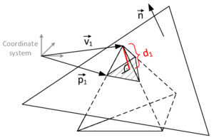
|
| Figure 57: Computation of the node distance to the plane - The perpendicular distance is the length of the projected vector onto the normal vector. |
A measure for the orientation of the structure is provided by the direction of the normal vector of the structure surface. In the framework of this monograph we will define that the normal vector of the structure surface is pointing outwards. This has to be ensured when the geometry is being created in order to guarantee that the sign of the distances is calculated correctly. In case of infinitely thin structures, which do not allow a distinction between inside and outside, it has to be ensured that the normal vectors of each mesh element are uniquely pointing into the same direction.
The determination of the distance sign is already implicitly contained in equation 7.3. This will be shortly shown in the following. Considering figure 58 the angle between the normal vector and the connection vector determines the sign of the distance.

|
| Figure 58: Sign of distance value - The angle between the normal vector and the connection vector of the intersection point and tetrahedron node determines the sign of the distance. |
The angle between the normal vector and the connection vector is related to the angle by:
|
|
(7.4) |
Together with equation 7.3 this results in:
|
|
(7.5) |
This implies that the distance is positive if the cosine is larger than zero and negative if the cosine is smaller than zero, respectively for the angle :
- : The fluid node is located outside the structure meaning that the normal is pointing into the direction of the node from a viewpoint of the structure surface. The distance value is positive.
- : In this case, the fluid node is located directly on the structure resulting in a distance value of zero.
- : The distance value is negative.
7.1.1.4 Assigning distances to fluid elements
The distance computation is done for all four tetrahedron nodes what finally results in a set of four real-valued distances for each tetrahedron element which is why the distances are called elemental distances in Kratos. It is important to note that the distances are computed locally for each tetrahedron element. This in turn implies that a node which is corner node of various intersected tetrahedron elements might have different distance values to the structure. Hence the elemental distances form a globally discontinuous function space. But as this is only the case for non-planar surfaces this problem will be picked up later again. Planar structures result in continuous elemental distance values.
The elemental distance values are assigned to the cut tetrahedron elements. Furthermore, it is convenient to have a flag which marks all cut elements as "split". This is done with the flag variable SPLIT_ELEMENT, which is set to true. This has the advantage that the set of split elements can be accessed later by just regarding the state of that variable. All the elements which are not cut, will keep the initially assigned distance value of at each tetrahedron node and the flag SPLIT_ELEMENT remains false.
7.1.1.5 Visualization of structure-approximated plane
In order to get feedback about whether the computation of the distances performs as expected and the presented algorithm can represent the structure properly, it is necessary to visualize the structure emanating from the distance values. So we want to visualize how the fluid "sees" the structure based on the given distances. This allows to e.g. detect fluid elements which are cut by the structure but due to a specific intersection pattern not considered by the algorithm. For a visualization, the structure triangle mesh is embedded into the fluid tetrahedra mesh as shown in figure 59.
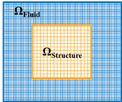
|
| Figure 59: Embedded structure in fluid domain - The structure mesh is embedded into the fluid mesh. Within this chapter we are interested in how the "fluid mesh sees the structure". |
The approximated structure is represented by the isosurface with a distance value of zero. This isosurface is supposed to be visualized with an additional postprocessing function, which will be called after the computation of the distances. The aim is to make it possible for the user to investigate the embedded structure as it is seen by the fluid solver. To this end the aforementioned postprocessing function triangulates the zero isosurface such that we get a separate mesh that can be imported in the program GiD. The principle of the function is shown in figure 60. Note that neither the function nor the corresponding mesh which is generated is needed in the computation of the sate equations. The sole purpose of this function is the visualization of the embedded structure.

|
| Figure 60: Flow chart for generation of the interface mesh - For each intersected element either one or two triangles are reproduced depending on the number of intersection nodes. |
The algorithm starts with a loop over all fluid elements. If the element is split, i.e. the flag SPLIT_ELEMENT is set to true, a loop over the respective tetrahedron edges is done, else the next fluid element is considered. For each of the six tetrahedron edges the distance values of the two corresponding edge nodes are checked mutually. The essential condition for computing a zero distance along the edge is a positive distance at the one node and a negative one at the other (i.e. the product of the distances is negative). This allows to conduct a linear interpolation to compute the location of the intersection point along the edge. Figure 61 shows the approach.
The position vector of the intersection point is then a vector addition of the weighted position vector of node and node with the respective ratio of distances
|
|
(7.6) |
It shall be emphasized that it is not possible to do an interpolation with this algorithm whenever a node has a zero distance. This requires further considerations that are discussed later in this chapter. The intersection points are computed for each tetrahedron edge whose corresponding nodes have opposite distance signs. Counting all intersection nodes, it is mathematically just possible to obtain three or four intersection nodes for a cut element when assuming that all distance values are different from zero. Three intersection nodes occur if one node has an opposite sign compared to the other three nodes. Four intersection nodes occur when each two nodes have an opposite distance sign.
As it is our aim to generate a mesh out of the set of computed intersection nodes, we need to think about how to create triangles based on the nodes. For the case of three intersection nodes, the situation is trivial as these nodes already form a triangle which can be easily added to the mesh model. For the case of four intersection nodes the generation of triangles is not obvious as the quadrilateral needs to be decomposed into two separate triangles. It becomes more clear when having a look at figure 62 which demonstrates the case of four intersection nodes. There is no geometrically correct automatism which defines two non-overlapping triangles by just connecting an ordered set of nodes without further considerations. Let us e.g. assume that the automatism defines to connect the points , and to one triangle and , and to another triangle, this would already result in two overlapping triangles and .
How to properly decompose the quadrilateral into two adjacent triangles? As shown in figure 62 on the left hand side, a vector is drawn from point to point and normalized:
|
|
(7.7) |
Now it is interesting to determine where the points and are located with reference to this connection vector. Based on this knowledge, one can construct two neighboring triangles.
First of all, we want to generate an orthonormal base as an auxiliary frame for referencing the location of the points and towards the vector . The notations follow figure 62. The normal vector which is perpendicular to the quadrilateral might be computed by means of the cross product of two connection vectors of the quadrilateral. But then we cannot ensure the correct orientation of the normal vector as it requires to point outwards, i.e. towards a positive distance value. Therefore it makes more sense to use the gradient of the distance values throughout a tetrahedron as an indicator for the orientation of the normal vector. The gradient can be computed by taking the gradient of the shape functions, which are assumed to be linear, and multiply it with the elemental distance vector:
|
|
(7.8) |
The definition of the linear shape functions within a tetrahedron can be taken e.g. from Felippa [52]. An additional vector completes the orthonormal basis and is computed such that it is coplanar within the plane spanned by the quadrilateral. This implies that it is perpendicular to and , resulting in following equation:
|
|
(7.9) |
Now, by means of the vectors and we can compute the angle of the connection vector related to and the angle of related to within the plane spanned by the quadrilateral. The procedure is as also visualized in figure 62 on the right hand side. If the angle is larger than zero, it implies that the point is located "above" , else it is "below". The angles can be obtained as follows:
|
|
(7.10) |
and
|
|
(7.11) |
Within these formulas, the numerator can be understood as the portion of the vector in the direction of and the denominator as the portion of the vector in the direction of . The ratio of the projections results in the tangent of the angle. Based on the angles, we can set up following overview to decide about the two triangles:
- If one angle is positive and the other negative, then the edge between and forms the shared edge of both triangles. This yields two triangles and .
- If both angles are positive, we need to compare them to each other to decide about the shared edge:
- If , then the edge between and forms the shared edge. This finally results in two triangles and .
- If , then the edge between and is the shared edge. The triangles and have to be created.
- If both angles are negative, we have to compare them to each other to decide about the shared edge:
- If , then the edge between and forms the shared edge. This finally results in two triangles and . Attention: these triangles have a different orientation compared to the case of having both angles positive!
- If , then the edge between and is the shared edge. The triangles and have to be created.
Doing these operations for each intersected tetrahedron, we finally get a mesh composed of triangles, which can be visualized in the postprocessor GiD.
7.1.1.6 Test case 1: Planar structure cutting one tetrahedron
Having all ingredients at hand, we have to prove that the algorithm is working correctly and can be applied reliably to approximate planar structures. A first self-evident test case would be to intersect a single tetrahedron and see how the algorithm is representing the intersection pattern. As a structure we will choose a simple triangle which is cutting the tetrahedron - once such that the triangle is intersecting the tetrahedron in three edges and once in four edges. For the two cutting test cases we expect the algorithm to generate a mesh once with one triangle and in the other case with two triangles. Furthermore we can check that the nodes of the generated interface mesh are positioned in the plane of the original structure triangle.
Let us first consider a structure triangle which is cutting a tetrahedron in 3 edges. The geometrical configuration is shown in figure 63.
The model parts of the structure and the fluid are read into one Python file by executing following command in the terminal:
|
Within the Python script, the distance function process is initialized with the input of the two model parts. This is done as follows:
|
|
In the first line, an object distance_process of the class CalculateSignedDistanceTo3D- SkinProcess is constructed. Then in the second line the function Execute is invoked which calls internally the distance computation algorithm. An additional function named GenerateSkinModelPart was implemented which handles the generation of a mesh containing the reproduced intersection patterns based on the distance values and can be called from the Python script.
When we test with the distance function the intersection pattern as shown in figure 63, we get the intersection mesh as depicted in figure 64 - composed of just one triangle.
The intersection recognition obviously works properly, also the triangle is reproduced correctly. In order to check quantitatively, that the visualized intersection triangle in figure 64 is directly coplanar in the plane of the original structure, we want to run a mathematical evaluation. If we can show that it is coplanar, it proves that the distance function approximates the structure exactly.
In order to do that, the distance of the three intersection points to the plane is computed. The intersection point is coplanar with the structure plane, if the distance is zero according to equation 7.2. The normal vector to the structure plane is calculated by determining the cross product of the triangle vectors and (notations see figure 56) as follows:
|
|
(7.12) |
The structure plane is then defined by this normal vector and a point which is located in the plane. Let us choose one of the triangle points of the structure, e.g. pojnt . Based on these information, we will check whether the three intersection points are located in the plane as shown in table 8.
| Int. point | |||
| 0,537616 | 0,337616 | -5e-08 | |
| 0,593535 | 0,193535 | ||
| 0,558047 | 0,258047 | ||
| 0,440965 | 0,240965 | -5e-08 | |
| 0,498233 | 0,098233 | ||
| 0,430977 | 0,130977 | ||
| 0,370729 | 0,170729 | 1e-07 | |
| 0,540459 | 0,140459 | ||
| 0,487278 | 0,187278 |
The second column describes the position vectors of the three intersection points. Together with one point of the structure triangle and the normal vector, the location with reference to the structure plane can be computed (fourth column). As one can easily observe, the scalar product is close to zero, what implies that all three intersection points are located within the structure plane. The calculation process for the case of three intersection points is therefore implemented correctly.
The second case is to move the tetrahedron in space such that the same plane as before intersects the tetrahedron at four edges. Such a configuration is shown in figure 65.
As we expect from the distance algorithm, it is able to generate two adjacent non-overlapping triangles out of the four intersection points as one can see in figure 66.
The check of coplanarity is also done for this intersection pattern and summarized in table 9.
Also in this case, the intersection pattern is recognized correctly by the distance algorithm and reproduced properly. By means of these basic test cases a structure plane can be constructed out of a multitude of triangles based on three or four intersection points per tetrahedra.
7.1.1.7 Test case 2: Rectangular plate in a fluid cube
Let us now see how a structure plate embedded in a meshed fluid cube is treated by the distance function. The plate is a suitable example to check whether the surface can be represented exactly as already supposed in the introduction. The geometrical setup is chosen as in figure 67. Beyond this, all the upcoming structure geometries - including the next chapters - will be embedded into this fluid cube with the same dimensions. This will help to provide a firm reference basis throughout the entire chapter.
| Int point | |||
| 0,537616 | 0,337616 | -5e-08 | |
| 0,593535 | 0,193535 | ||
| 0,558047 | 0,258047 | ||
| 0,570883 | 0,370883 | 5e-08 | |
| 0,583658 | 0,183658 | ||
| 0,544877 | 0,244877 | ||
| 0,528592 | 0,328592 | 0 | |
| 0,422803 | 0,022803 | ||
| 0,330404 | 0,030404 | ||
| 0,440965 | 0,240965 | 5e-08 | |
| 0,498233 | 0,098233 | ||
| 0,430977 | 0,130977 |
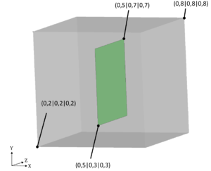
|
| Figure 67: Structure plane embedded in a fluid cube - This figure shows the geometrical configuration in which a plane (green) is embedded in a cube (grey). |
First of all, the fluid cube is discretized with tetrahedra elements. The structure plane can be exactly discretized by just two adjacent triangles. Such a coarse discretization is possible as the intersection pattern detection does solely depend on the fluid discretization. The finer the fluid mesh is chosen, the finer the structure-approximated mesh will be. In the course of this chapter, we will go further into the influence of the fluid discretization.
Applying the distance algorithm to the plane embedded into the cube, the mesh as shown in figure 68 can be obtained.
The left figure shows the original structure plane, which is filled with green color to frame the area which the distance function is expected to approximate by a mesh of triangles. The grey meshed surface is the one which is obtained by the distance function. At first glance, the mesh does not exactly coincide with the original structure throughout the entire plane. It is noticeable that along edges the structure can not be approximated optimally, some triangles are overlapping the plane edges and some parts close to the edges can not even be captured by any intersection pattern. This points to a certain deficit of the distance algorithm which was not yet discussed. As this problem is a general drawback of the embedded approach, chapter 7.1.3 will discuss why the edges can not be captured by the algorithm and how the approximation of the structure along the edges can be improved.
Within this section we want to concentrate on the representation of the plane-internal region. If we consider the side view of the approximated mesh in figure 68b, there is a pure straight line which reveals that all triangles of the mesh are coplanar in the original structure plane. This is a quite significant fact as it allows to claim that the structure plane can be described exactly by means of the distance function. Furthermore, one can derive that the theoretically discontinuous distance function can describe a plane surface continuously. If this was not be the case, then we would be able to recognize small jumps in the distance values between neighboring elements leading to a humpy plane representation.
However, another obvious deficit is dominating in figure 68a. In the mesh interior there is a clear void without any triangles. Therefore it can not be the influence of the edge-near problem zone. Instead the reason turned out to be that some nodes of the fluid mesh coincide with the structure plane. This leads to an intersection pattern with one, two or even three intersection nodes directly located on a tetrahedron node as shown before in figures 55a and 55b. A simplified 2D visualization of this situation is shown in figure 69.
Basically, all the visualized fluid elements are marked as split and the elemental distance vector contains one or two zero distance values. The problem with zero distances is that emanating from these structure-coinciding nodes no intersection point can be interpolated along the edges to that node as this requires a negative and a positive signed distance value. This implies that within the tetrahedron no triangle can be generated as no intersection point can be computed. Related to figure 68a there is one node which is coinciding with the structure plane. All tetrahedron which share this node will be neglected in the visualization function and therefore a hole is arising. A remedy for this is presented in the following section.
7.1.1.8 Strategy to eliminate zero-distance values
As zero distance values can not be treated for later computations it is obvious to slightly alter these distance values such that the error which is made is negligibly small. This means geometrically that the structure is slightly moved locally at these nodes. The question is which value should be assigned to these node that the structure is still approximated correctly. Let us again have a look at figure 69. We will define the rule that all nodes with zero distance are moved "away from" the structure, i.e. get assigned a small positive value. In this case, the fluid elements on the positive side of the structure will have positive distances at all the nodes. Therefore no intersection point can be computed as all nodes are "outside" of the structure such that these elements are not split any more. The elements on the negative side of the structure would now have nodes "inside" as well as "outside" of the structure. These elements are then still marked as split.
Assigning a small negative value to the nodes with zero distance instead would also solve the problem. In this case, the elements on the negative side would not be split any more. We will choose the first method and assign a small positive distance value to these nodes. The result is shown in figure 70.
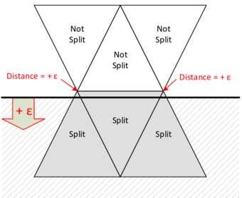
|
| Figure 70: Strategy to eliminate zero-distances - The nodes with zero-distances are assigned to a small increment which effectively corresponds to a locally moving the structure. |
As distance increment an absolute value of is chosen. After the distance function was extended by this method, the plane now looks as follows (figure 71).
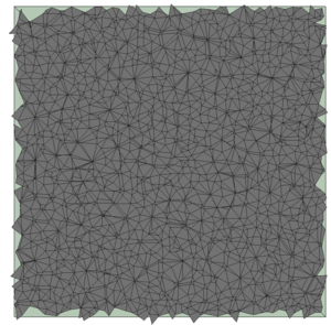
|
| Figure 71: Representation of the plane after eliminating zero-distances - Compared to figure 69 the hole does not appear any more. |
The region around the node with a zero-distance is now completely closed as all the tetrahedra are able to represent the intersection pattern. The difference can be better shown in a direct comparison of this region - once without the local structure movement (figure 72b) and with the zero distance correction (figure 72b). The right figure shows clearly that there was one node with a zero distance which is now forming numerous triangles to close the hole.
This method conveys more advantages which go far beyond this demonstrated purpose. In the embedded method the nodes with zero-distance can be physically seen as part of the fluid and structure at the same time. There is no clear distinction between the properties which should be assigned to this node. How to treat these nodes in the formulation of the embedded approach? The set of modified shape functions of the split fluid elements - as explained in chapter 2.2.4.2 - is based on a clear distinction of each node to either fluid or structure, which is provided in any situation by the just discussed local interface-movement approach.
7.1.1.9 Test case 3: Cube structure in a meshed cube of tetrahedra
Let us now consider a volumetric structure which has large planar surfaces. As side planes of such a cube should be treated in the same way as the planes considered in test case 2 by the distance function we expect the surfaces of the cube to be represented exactly as well. It will have deficits at the edges as the distance function can not compute the borders of the plane accurately.
As a setup the cube in figure 73 is chosen and will be embedded into the same fluid cube as in the previous test case.
When we apply the distance function to this setup, we will obtain the results shown in figure 74. In the left figure 74a - a smooth visualization of the reproduced structure mesh - one can see clearly that the internal domain of each of the side plates of the cube are describing a planar surface.
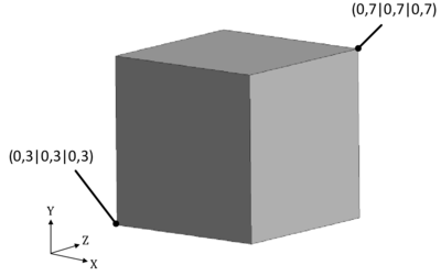
|
| Figure 73: Dimensions of the structure cube - This figure shows the geometrical setup of the cube which will be embedded in the fluid cube. |
There are no holes which would indicate deficits of the distance function. A problem is still the region around the edges of the cube - which can be traced back to the problem which was already discussed before. Around this area there are tetrahedra which are not split completely by the structure and therefore result in intersection patterns which are not yet considered. A workaround will be discussed later in section 7.1.3 which is especially dealing with this topic.
In order to inspect the representation of the side plates more in detail we can have a look at a cutting plane perpendicular to a side plate which is compared to the original structure close to the edge as shown in figure 75. The contour line of the structure-approximated mesh is shown in the left figure. On the right hand side one can see the original structure overlapping the structure approximation. It is clearly visible that the surface of the side plates can be represented exactly up to a certain point close to the edge, where the two plates are roughly connected via an element.
By means of these test cases we could prove the correct performance of the distance function applied to planar surfaces. Where the corresponding functionality is implemented within the overall process flow from figure 4 is shown in figure 76. As there were just changes in the block of the distance computation, only the respective block is depicted here. All added functions are highlighted in orange.
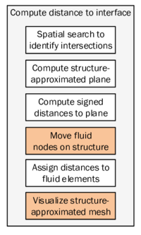
|
| Figure 76: Updated flow chart of distance computation - The additional functions which were added to the distance algorithm within this chapter are highlighted in orange. |
7.1.2 Geometric approximation of curved structure surfaces
As opposed to planar structures, a curved surface can principally not be approximated exactly by a set of triangles. This is a general error with the discretization using finite elements. Therefore the distance function will - no matter how sophisticated the algorithm is - never be able to represent the structure accurately. Rather more we need to find a way to approximate such structures as accurate as possible. The question of how to approximate a curved structure as exactly as possible is discussed within this chapter. To test the performance of our implementation, we will choose a sphere which is characterized by a constant curvature along the entire surface. The sphere forms a basic benchmark which will be applied frequently with the embedded method in the course of this monograph.
As already mentioned, a curved structure can not be represented exactly by a set of distance values. A descriptive 2D example is shown in figure 77. Here, the curved geometry of the structure can not be resolved within the triangle by just three distance values (in 2D) - an error is made at this stage.
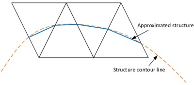
|
| Figure 77: Approximation of a curved structure (2D) - The structure contour (orange) is represented by the fluid elements (triangles) by a collection of lines (blue). |
Particularly the normal vector representing the orientation of the structure is changing its direction within the fluid element. So the plane to which the distance values are computed is not exactly defined by default - we need to develop a strategy to approximate the structure within a fluid element as good as possible. Another important problem which should be mentioned here is the case of four intersection nodes. In case of planar structures we could be sure that the four intersection nodes are located in one common plane - the structure plane. This is not the case anymore with curved structures. So the plane needs to be approximated now. An appropriate method is presented in the following.
In order to analyze this properly, we will go through the basic intersection patterns which were discussed in the previous chapter and see how the distance computation needs to be adjusted. These are the cases of one up to four intersection nodes. Having just one intersection node, the distance computation is still straightforward as the normal vector of the touching structure element can be used to define the plane to which the distances are computed (see figure 78).
For the case of two intersection nodes (see figure 79) we have now the characteristic that the normals at the intersection nodes are pointing to different directions. Having in mind that we want to treat fluid nodes with zero distances separately in a postprocessing step, like discussed at the end of the previous chapter, we need ensure that the two cut corner nodes of the tetrahedron have a distance value of zero. Therefore we at this point enforce these nodes to be zero.
The distance values of the other two nodes are computed as follows. It might be a simple approach to compute the shortest distance of such a node to the connecting edge of the intersection nodes. But then we would not involve the structural surface information which might introduce a unacceptable error. In order to consider the structural information, a good approximation would be to define the normal vector of the structure-approximated plane as an average of the normal vectors and . The point of the plane is calculated by averaging the two intersection points and . In the following we will call the point of the structure-approximated plane and the normal vector .
For the case of three intersection nodes (see figure 80) we already have the structure-approximated plane at hand since we can just take the triangle that is formed by the intersection nodes. By doing so we can ensure that the structure-approximated plane is directly passing through the intersection nodes.
As a base point for the structure-approximated plane we assume one corner node of the triangle, i.e. any of the intersection nodes such as . The normal vector of the plane is the normal vector of the triangle at the same time. It can be computed from the cross product of the triangle edges:
|
|
(7.13) |
As the orientation of the normal vector is not coupled to the structure surface but just linked to the triangle geometry it is not definitely sure that the normal is pointing "outwards". Therefore an additional condition needs to be added which checks the scalar product of the computed normal vector and one of the normals of the structure at an intersection node. Only in case the scalar product is negative, which means the normal vector is pointing "inside", the normal is multiplied by .
Having four intersection nodes it can not be ensured that all nodes are located in one plane. There are different methods to take this into account. A quite simple approach would be to compute the average of the intersection nodes as a base point of the structure-approximated plane and the average of the normal vectors of the structure at the intersection nodes. The implementation would be straightforward and the computational effort would be small. But as the geometry approximation is one of the key deficits compared to the ALE approach, we want to implement a method that allows an as accurate geometry representation as possible. Unfortunately the aforementioned averaging is too simple in that regard. In order to find a plane which is approximating the structure the best, we perform an optimization that fits the approximation plane into the split element such that the distance to all of the intersection nodes becomes a minimum.
Therefore we first note all the equations which define the distance of the intersection node to the plane we are looking for (according to equation 7.3):
|
|
whereas the position vector defines the position of a point that is located on the plane and is the position vector. We can also rewrite this set of equations in matrix form:
|
|
(7.14) |
whereas the matrix collects the connection vectors between the intersection nodes and the base point of the plane:
|
|
(7.15) |
Based on these equations we want to minimize the sum of the four distance values to the plane which we are looking for. As the distance values can have positive and negative signs it is appropriate to formulate this optimization problem as a least squares problem. The objective function hence reads:
|
|
(7.16) |
In the last equation the matrix product was summarized to a matrix . Due to the fact that the plane is defined by two parameters (base point, normal vector), we will fix the base point and look then for that normal vector that results in the least squares of the distances. A good choice for the base point is the mean of all four intersection points:
|
|
(7.17) |
The normal vector as design variable for the optimization problem is normalized in the distance equation. But with regard to the solution of the problem it would be more convenient to directly compute a normal vector which has length . In the optimization problem we can enforce this condition as an equality constraint:
|
|
(7.18) |
Based on equations 7.14, 7.16 and 7.18 we can formulate the optimization problem as follows:
|
|
(7.19) |
This constrained quadratic optimization problem is an overdetermined system as we have five equations (objective function with four distance equations and the constraint equation) to solve the three unknown components of the normal vector . We will solve that problem by first computing the Lagrangian function using a Lagrangian multiplier :
|
|
(7.20) |
The stationary point of can be obtained by partially deriving with respect to and :
|
|
(7.21) |
|
|
(7.22) |
The first equation can be rearranged such that we gain the following eigenvalue problem:
|
|
(7.23) |
whereas denotes the eigenvalue of the matrix and the corresponding eigenvector. Having this in mind the equation can be multiplied with . By using equation 7.18 we eventually get:
|
|
(7.24) |
As the left hand side characterizes the objective function ( see equation 7.16), we can deduce from this equation that the function is minimized at the eigenvector which corresponds to the minimal eigenvalue of the symmetric matrix . To solve the problem we use the given features in Kratos which returns the ordered eigenvalues and corresponding eigenvectors. The algorithm is based on the iterative Gauss-Seidel method.
The eigenvector which corresponds to the minimal eigenvalue yields the normal vector of the plane which gives the least squares of the distances of the intersection nodes to that plane. Although this method appears to be quite promising and accurate, it is computationally very demanding as this iteration for computing the eigenvalues has to be done for each fluid element which is cut at four edges. It is therefore much costlier compared to just taking e.g. the average of the normal vectors.
Now, that the algorithm is also able to approximately compute the distance to curved structures, the code can be principally applied to a sphere in order to review the performance and deficits of the distance function. The sphere which is embedded into the fluid cube is shown in figure 81. First of all, a rather coarse fluid mesh (8e4 tetrahedra) is used to better visualize potential weak points of the distance function.
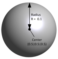
|
| Figure 81: Setup of the sphere - This sphere will be embedded into the fluid cube and tested with the distance function. |
The result which is returned by the distance function is shown in figure 82.
Generally the sphere can be reproduced with the current distance algorithm, the curvature of the sphere can be described with an acceptable accuracy, whereas a finer fluid mesh would be able to even resolve it much better. However, when looking at the figure, we find two polygonal holes in the mesh marked with red arrows. That is a clear sign for the occurrence of a certain intersection mode which is not covered in the algorithm. Therefore it is advisable to detect the tetrahedra which are responsible for causing these holes in order to reproduce the intersection pattern. The images in figure 83 show such a situation for one of the holes.
The right figure shows the reproduced sphere including the tetrahedron which is not able to detect the intersection pattern. As it is hardly visible on the figure, it is noted that there is also a second adjacent tetrahedron which can not detect the given intersection pattern. Now it makes sense to see the tetrahedron related to the original sphere geometry in order to analyze the intersection pattern (see figure 84).
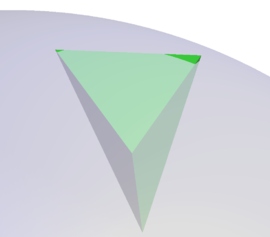
|
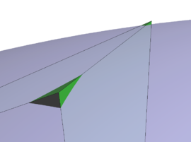
|
| (a) Perspective 1 | (b) Perspective 2 |
| Figure 84: Intersection pattern along the sphere surface - Both figures show the same situation in which the tetrahedron exhibits five intersection nodes. | |
Examining the figures one realizes that the tetrahedron is cut in six points, whereas one edge is cut even twice. Such a case is not possible for planar structures and arises for curved structures as the structure is "leaving" the tetrahedron and "entering" it again along one edge. Furthermore we can not describe more than four intersection points with the set of four distance values. So the question is, how can we encounter such intersection patterns?
Let us break down the situation to the most simple situation. Therefore a two-dimensional visualization is chosen. An abstract intersection pattern which is similar to that encountered before is shown in figure 85.
The left element in the figure has the four intersection nodes to , whereas and are located on one edge. The right element shares these two intersection points with the left one. Considering the element on the right there is no way to represent this protruding curved element of the structure with a single line. The element can not detect what happens with the structure in the element-internal domain. With the distance function we can not handle such detailed information. Considering the element on the left hand side it is also difficult to directly define the structure-approximated line. The main reason for this is that the element practically "sees two structures" - once the structure segment between and and once the structure segment between and . However a distance value can only describe the distance to one specific line. This implies that a strategy has to be developed to face such cases - an error will be made by default such that a good compromise has to be found.
As already discussed, the small structure segment which traverses the right element can not be described by the distance vector. A line could be drawn through the intersection nodes, but these would cause that the two corner nodes of the cut edge get a distance of zero and one node gets a positive distance. But the reproduced structure would not represent the curved structure at all - a large error would be made. A better way would be to assume that we neglect this very small structure segment and consider this element not to be cut. The error would be rather small. This brings the advantage that we can form a secant line in the left element and therefore "cut" the curvature. A way to do this is to compute a line which minimizes the distances to all the intersection nodes. This is the same approach as done for four intersection nodes - but in this case with more intersection nodes. The advantage is that we can use the same algorithm, whereas the eigenvalue computation would be more costly. As this intersection pattern is quite rare we can neglect, however, the additional computational effort. Eventually one obtains the following structure approximation (figure 86).
Projected to the three-dimensional case this would imply that as soon an element is cut twice along one edge, the element is neglected and not marked as split. The other element takes all these intersection nodes to compute an approximated plane based on the optimization problem explained before.
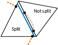
|
| Figure 86: Approximation of the structure for the intersection pattern shown in figure 85 - The structure (orange) is approximated in the left element by the blue line and the portion of the structure in the right element is neglected. |
Having implemented a strategy to handle the stated problem we can see how this influences the approximation of the structure by the distance function. First we will examine the region containing the hole which was considered in figure 83. After applying the updated distance function to the sphere, we obtain the results shown in figure 87.
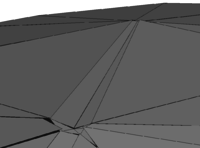
|
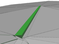
|
| (a) Intersection pattern can be captured | (b) Visualization with the respective tetrahedron |
| Figure 87: Corrected defect in the reproduced sphere - By extending the current algorithm the defect hole as shown in figure 84 can be resolved. | |
The left figure proves that the tetrahedra (shown in the right figure) now realizes the intersection pattern and reproduces the structure with a large accuracy. The entire sphere is visualized in figure 88.
Comparing the sphere to the previous result, the main deficits could be resolved with the presented strategy. The holes could be closed and this even with a very good accuracy. When having a closer look to the left figure, one might realize small white spots. Zooming into such a spot, it becomes clearer where these white areas come from (see figure 89).
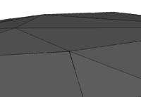
|
|
| (a) Part of the sphere | (b) Zoom to a specific node |
| Figure 89: Discontinuity of the elemental distances demonstrated at one node | |
The right figure shows the discontinuity of the local elemental distance vectors which is a consequence of the fact that we use a discontinuous distance function where a certain node can have different distance values - depending on which element containing this node is considered. Before we were not faced with this problem as planar structures can be described exactly and continuously with the distance values. The effect can be described visually by means of figure 90 which is based on the setup shown in figure 87.
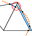
|
| Figure 90: Discontinuity of elemental distances - This figure demonstrates the discontinuous representation of the facets at the spot which is marked with a red circle. |
As we approximate the structure with a plane in the right element, we can not ensure any more that the plane is directly passing the intersection nodes. The adjacent element, however, allows this approximation and therefore a "jump" in the structure-approximated mesh is occurring. This is an error which can be led back to the intended choice of using elemental distances, i.e. a discontinuous distance function, for the approximation of the embedded structure. So the above discussed approximation error can not be avoided be default. Though, the error can be decreased by choosing e.g. a finer fluid mesh. Also, a finer fluid mesh would decrease the error made by the approximations to the curved structure.
Let us investigate the influence of the refinement of the fluid mesh more in detail as this obviously of utmost importance for the accuracy. The fluid mesh which was applied before was based on a rather large element size of (using elements). When we refine the fluid mesh globally and therefore reduce the elements size to (using elements), the curvature of the sphere can be reproduced much better by the distance function as clearly shown in figure 91.
Comparing this to the mesh we gained before (figure 88) the improvement gets obvious. The curvature can be described perfectly and there are no visible defects. As it is hard to evaluate this improvement visually we want to measure this improvement quantitatively. The sphere is well-suited for setting up a quantitative measure as we can describe the shape of the sphere mathematically without any big effort. It is therefore possible to compute the analytic distance value of a node to the structure. The radius on which the node of an element is located with respect to the sphere center is described by the sphere equation:
|
|
(7.25) |
Comparing this radius of the node to the radius of the sphere yields already the analytic distance of the node to the structure:
|
|
(7.26) |
The absolute error which is made can be formulated via the difference between the analytic distance and the approximated distance computed with the distance algorithm:
|
|
(7.27) |
For each element these errors can be summed up over the four nodes resulting in the elemental absolute error . We will sum up the squared errors in order to penalize large deviations more than small deviations:
|
|
(7.28) |
After all, the overall absolute error can be quantified by taking the sum over all split elements of the fluid mesh and taking the root over the entire measure:
|
|
(7.29) |
In order to get more useful error values and provide the possibility to compare the error measures with each other the absolute error is normalized by the overall analytic distance values resulting in the relative error measure:
|
|
(7.30) |
Based on this formula we will do some studies to evaluate the error depending on the element size of the fluid mesh. This will not serve as a universal rule as we apply it to the specific test case of the sphere which can be treated properly by the distance algorithm. But it should give a rough idea about the performance and accuracy of the distance algorithm and provides a good measure to compare external distance algorithms with the one implemented within this monograph.
For the study we will vary the element size between a very coarse mesh and a very fine mesh. Nine samples of different element sizes are chosen and finally collected in one chart which is shown in figure 92.
The relative error of the distance values is increasing linearly with the mean size of the fluid elements. When using a really coarse mesh (e.g. ) the relative error has a value of more than 0.25 denoting an error of more than 25 % - a rather large deviation from the sphere structure. By reducing the element size the error can be linearly reduced down to a value of 3 % for the smallest used element size in the framework of this study. But already an error of 10 % and below sounds promising and will be used to define a rough rule of thumb concerning the maximal element size. An error of 10 % can be reached with an element size of approximately for a sphere with radius .
Decreasing the element size will of course also increase the number of cut elements in the standard fluid cube that is used for the interface treatment studies. One interesting question in this context is, how does halving the element size influence the number of split tetrahedra in the fluid cube? Figure 93 shows a corresponding study in a log-log plot.
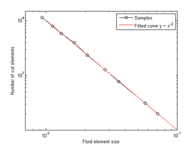
|
| Figure 93: Relationship between the number of split elements and the element size - There is a quadratic relationship emphasized by the red trend curve. |
The log-log plot is used in order to impressively show the quadratic relationship between the number of split elements and the element size. This implies that in order to halve the relative distance error the elements size has to be halved, but the number of elements will be quadrupled by this. So the computational effort for computing the intersection patterns for all the split elements is increasing quadratically when the error shall be reduced by .
7.1.3 Geometric approximation of sharp-edged structures and thin volumes
The previous two chapters have shown the implementation of an efficient algorithm which is capable of representing large-scale planar or curved structures with high accuracy. However, these chapters have also shown the limits of the algorithm. Those limits especially arise when complex variations of the structure shape occur within a single fluid element and can not be represented in detail by a set of distance values. In particular strong discontinuities or large curvatures in the structure (edges, corners) as well as very thin two-sided structures are severe cases which can not be handled by the current distance algorithm. In the following we will discuss the proper treatment of these cases and propose methods that are able to deal with these cases in a way that the induced error is minimized up to an acceptable limit.
In the first chapter we have already demonstrated that the edges of a cube can not be represented exactly (compare figure 75). Therefore an aim of this chapter is to properly treat the edges and corners of the cube. The edges of the cube cause troubles as two surfaces with different orientation (the normal vectors are perpendicular to each other) are joining at an edge. A tetrahedron at this location is not able to describe both surfaces at the same time. Corners are even more problematic because three surfaces with different orientation join in one point. In fact, we can completely concentrate on these problem zones as the surfaces are already represented exactly by the current algorithm. Therefore a cube is a suitable test case.
A very representative example for thin two-sided structures is a thin wing structure given by the front wing of a Formula 1 car (see figure 94).
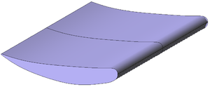
|
| (a) Side view |

|
| (b) Cross surface |
| Figure 94: Wing structure - The figure shows two views of a part of the front wing of a Formula 1 car. |
This test case covers most of the critical configurations we want to analyze within this chapter. First, the structure is thin throughout the entire structure, but with an varying thickness. At the end of the wing (left hand side in the figure) the structure is getting very thin and connecting the upper and lower surface with a strongly curved surface. This is a special challenge for the algorithm as there two separate surfaces (upper and lower) are joining. The main upper and lower surface of the wing are curved surfaces whereas the side plates are planar. There are also sharp edges at the transition between the main surfaces and the side plates. All in all, this example contains many geometric features which are interesting to analyze with the distance function.
As starting point, the distance function in its current state is directly applied to the wing structure without any adaptions. The result is presented in figure 95.
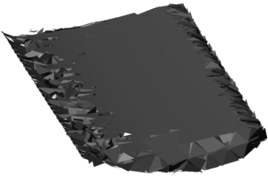
|
| (a) Side view |

|
| (b) Cross surface |
| Figure 95: Structure-approximated mesh of wing structure - The shown structure is a result of the application of the original distance algorithm. |
The main upper and lower surface of the mid section of the wing can be represented very good. However, as expected, the algorithm is not able to treat the front and rear wing structure correctly. The cross section in figure 95b shows this clearly. In the region in which the wing thickness falls below a certain limit, many misaligned mesh elements occur and lead to a bad resolution of the overall structure. If we want to explain this effect, we have to look at the intersection pattern of the elements which cause that problems. The following figure 96 shows the corresponding situation at the rear wing section. The (green) tetrahedron is cut by the upper as well as the lower surface of the wing and approximates the structure with the red-framed triangle.
The problem is obvious when noting that there are tetrahedron edges which are cut twice - once by the upper and once by the lower wing surface. As explained in the previous chapter, the algorithm takes all the found intersection points and computes a plane with minimal distance to these points. Having two double cut edges - as in the current situation - it is probable that the plane is aligned such that the two surfaces are connected. This is, however, not correct and the consequence will be that the wing structure at this point is approximated by an element protruding from the wing surface rather than one that forms the wing surface.
In order to better demonstrate the problem and develop an efficient solution, we reproduce the just discussed intersection pattern with an abstract graphic simplified to 2D (figure 97a).
The element in the middle has four intersection points, whereas two are located on one single edge. So the question is how does the current distance algorithm reproduce this intersection pattern? And the answer is, without any improvements, the structure is reconstructed by a cross line (see figure 97b, which is comparable to the misaligned red-framed triangle in figure 96.
As already mentioned, there is no way to represent both structure surfaces within the intersected fluid element at the same time. A strategy has to be formulated to remedy this fundamental problem.
Up to this point we were not caring about the distinction between infinitely thin structures and volumetric geometries. So far, the two-sided volumetric structure is locally just collapsed to a one-sided membrane structure. That implies, however, that one side of the fluid element gets positive distance values whereas the other side gets assigned negative values - even if all nodes are located outside of the structure. This distinction can be effectively handled with the continuous distance function which finally defines the nodes to be inside or outside of the structure. The underlying technology is the so-called ray tracing which was already introduced in chapter 2.2.4.1. This allows to detect volumetric structures and the position of the nodes related to the volume. If the ray tracing detects a node to be located within the structural volume, the sign of the nodal distance is negative and stored in the nodal variable DISTANCE, otherwise it is positive and stored in the same nodal variable.
That is very useful in the mentioned case when the two-sided structure is locally reduced to a membrane structure. The discontinuous elemental distance function assigns positive distance values on the one side and negative on the other side. The ray tracing method is doing the following: the sign of the nodes which are assigned to a negative distance are just switched to a positive sign and stored in the DISTANCE variable. Later the nodal DISTANCE values can be used to detect all the fluid nodes inside the structure and therefore treat them differently as opposed to the nodes outside the structure.
The remedy should be capable of at least not disturbing the flow along the structure surface (as done by the current code) and ensure that the flow can not cross this structure. That implies to align the structure-approximated plane such that it roughly maintains the orientation of the surfaces. One way to do this is to ensure the proper representation of one of the structure sides (figure 98). Therefore it is possible to prevent a cross-structure flow of the fluid.
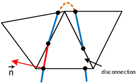
|
| Figure 98: Proposal for representation of intersecting two-sided structure - The idea is to describe one of the surfaces properly. However this causes a disconnection on the other side. |
The implementation is straightforward as the structure-approximated plane is defined by one of the intersection points along the double cut edge and the normal vector of the structure element which is cutting the element at this intersection point. There seems to be a disconnection at the opposite structure side. However, these approaches seem to solve efficiently some of the previous problems. There are further different intersection patterns to which these approaches can be applied. The corresponding intersection patterns are shown in figure 99.
The upper figure 99a shows the case in which the tetrahedron is cut twice along one edge and the lower figure 99b shows a tetrahedron with even three double cut edges. Let us e.g. have a look at the latter intersection pattern which can be basically broken down to the configuration shown in figure 100a. The distance algorithm would approximate the structure as follows - without the just presented strategies (figure 100b).
Again one can clearly observe the misaligned elements. Applying the proposed approach, one of the two surfaces will be represented by the structure-approximated plane leading to an interruption in the other surface. Figure 101 shows this result.
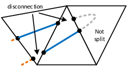
|
| Figure 101: Proposal for structure-approximation of the situation shown in figure 100 - Only one surface of the two-sided structure is represented with the distance function. |
The algorithm is not able to always refer to the same surface of the structure for each element. This would require further effort in programming which we do not want to pursue here. Applying this algorithm with the proposed strategy to the entire wing structure shows promising results (figure 102).
The thinning region of the wing cross section does not exhibit any cross-aligned elements connecting the two sides of the wing. The structure can be clearly approximated - also close to the trailing edge. This can be ensured by the approach which concentrates on the reproduction of one structure side. A closer look to the trailing edge reveals some apparently misaligned elements having various orientations. This can be explained with the small rounding at the trailing edge which is discretized by structure elements with different orientation. The mentioned disconnection or rather "holes" within the structure can not be seen in the cross section visualization, but in figure 103.

|
|
| (a) Cross section | (b) Zoom to the trailing edge |
| Figure 102: Wing model tested with the proposed approach - The applied approach is illustrated in figure 101. | |
The interruptions in the structure are visible. It is important to note, however, that nevertheless the fluid can not cross the wing structure with this approach. This will be proven later in chapter 7.2.1. Indeed the presented method is visually advantageous and easy to implement, it is physically more accurate to approximate the two sides of the thin structure by means of an averaged plane which is located in between the two-sided structure. The orientation of the plane also arises from an average of the surface normals. What we want to achieve is the result shown in figure 104.
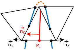
|
| Figure 104: Improved proposal for the representation of intersecting two-sided structure - The idea is to describe a plane in between the two structure sides with an averaged orientation. |
The base point of the structure-approximated plane is then computed as a mean of all the intersection points of a double cut edge. The normal vector is also computed as the mean of the structure normals at these intersection points. It has to be noted that the normals of the structure are always pointing "outwards", which implies that the normals of the two sides in a thin structure are pointing into opposite directions. Therefore one of the normals should be reversed before computing the mean. The implementation is according to the following pseudocode:
for in do
- for in do
- end for
- if : then
- Reverse this normal vector
- end if
end for
mean()
mean()
First, all the double cut edges are searched and the corresponding intersection nodes and normal vectors of the structure are stored in containers. Finally, the base point of the structure-approximated plane is computed as a mean of all nodes within the container. The normal vector of the plane is also computed as a mean of the container comprising the normal vectors.
This approach results in a mesh which shows elements in the middle of the wing structure as illustrated in figure 105 although not having any misaligned elements. The front view of the structure approximation indicates the apparent “holes” in the structure which, however, do not allow the fluid to cross as explained already in the previous approach.
This proposed averaging of the two-sided structure appears to be the best compromise which is achievable geometrically. However we should note an important fact which indicates a general drawback of the embedded method. Reducing the two-sided structure locally to a one-sided structure leads to geometrical discontinuities as illustrated in figure 106.
Such a structure approximation of the boundary leads to physical difficulties when a flow separation at the tip of a thin structure shall be computed. The embedded approach is very inconvenient in this concern and does not allow to compute the forces of the flow onto the structure accurately as this would require to resolve the boundary layer much better. Those discontinuities can not be avoided due to the presented problems but we can try to reduce it to a minimum by locally refining the fluid elements which encounter the inability to represent both surfaces at the same time. If such an element can be divided into two smaller elements whereas one is able to resolve the “upper” side of the thin structure and the other is able to resolve the “lower” side, the situation could be improved locally. Such refinement strategies are presented at the end of this chapter. First we need to analyze the cube as there are further key issues which have to be considered.

| |
| (a) Side view | |

| |
| (b) Front view | |
| Figure 105: Wing model tested with the proposed approach - The applied approach is illustrated in figure 104. | |
7.1.3.1 Geometric treatment of cube edges
Let us investigate the resolution of the cube edges with the just developed method. If we applied this method to the edge-close region of the cube, we would encounter the problem shown in figur 107.
The element in the middle is cut twice along one edge such that the algorithm is executed as just presented for thin structures. The algorithm will compute a plane which averages the normals and the intersection points along the double-cut edge leading to a misaligned element. We rather like the element to provide a connection between the two surfaces of the cube such that we get an edge as it was already achieved in the first section of this chapter (see figure 75) and as it is shown in the following figure 108.
This, however, requires to distinguish in the code between cases in which the structure surfaces should be linked and cases in which a mid-plane should be computed (with thin structures e.g.). The decision of which approach should be used strongly depends on the geometrical change of the structure within one element. If the structure triangles change their orientation within a single element just slightly (e.g. a sphere), it is best to to approximate the structure with a plane through the intersection points and compute the minimal distance of all intersection points to that plane (as explained in the first section). If, however, the triangles change their orientations strongly (distinct geometrical features within one element) and even have large opening angles (thin structures), a mid-plane based on the intersection points along the double-cut edge needs to be computed.
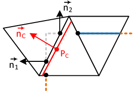
|
| Figure 108: Treatment of cube edges - The structure-approximated plane is supposed to provide a link between the cube surfaces which yields an approximated edge. |
Therefore it seems to be convenient to compare the normal vectors of the structure elements which are cutting an edge of the fluid element twice. If the angle between the vectors is larger than a certain limit, the mid-plane computation is done, else the minimal plane is computed. A proper limit is hard to set, but it would also be an idea to leave the decision to the user as it sometimes might depend on the application example. Here, we will set the limit to an angle of what allows a proper representation of the cube edges (angle of normal vectors which is smaller than the limit) and the thin structures (angle of normal vectors around which is larger than the limit).
Figure 109 summarizes the final state of the distance function with its approaches and improvement strategies. In doing so, the figure shows the core part of the distance function dedicated to the computation of the structure-approximated plane.
7.1.3.2 Towards efficient refinement strategies
As roughly explained above, the distance function can not handle complex geometries e.g. thin structures accurately due to the intrinsic definition of the element-wise distance function. An efficient approach to reduce the drawbacks of the embedded method with certain intersection patterns is to apply refinement strategies like the so-called Adaptive Mesh Refinement as presented in the paper of Rossi, [53]. The latter algorithm basically refines all the fluid elements which are cut, i.e. whose flag SPLIT_ELEMENT is set to True. Its principal procedure reads:
for in do
- if then:
- end if
end for
This function has to be called after all cut fluid elements are tagged accordingly. Without any improvements, however, this leads to an immense computational effort. Nevertheless we take this strategy into account in case the overall geometry of the structure is not approximated well due to a comparably coarse fluid mesh. We will keep this idea in mind for later considerations.
Instead of refining all cut fluid elements, it would make more sense to treat only those elements which have crucial problems to properly represent the structure and leave the other elements unchanged. Following this idea, however, it remains to decide about which of the cut elements shall be refined in order to approximate the structure in an efficient manner.
A cut fluid element that indeed needs to be refined is given if it has double-cut edges. As already discussed in previous paragraphs this double-cut edges are a sign for strong local geometry changes. A local refinement of such elements hence allows to further resolve structural details.
A second indicator to decide whether to refine a cut fluid element or not is given is the change of the normal vectors of all structural elements that are enclosed by the cut element. If the structure is slightly curved or even planar, the change of normal vectors is small, i.e. no refinement is necessary. If the curvature is large or the structure changes its direction within an element, it makes sense to refine this element. Such cases can be detected by comparing the normal vectors of the corresponding structure elements to each other and if any pair of vectors is found that have an angle of e.g. to each other, this element will be refined.
A third cases in which we want to perform a refinement is the case in which a fluid element is just slightly touched by the structure resulting in just one or two split edges. Before it was not possible to represent the structure based on such intersection patterns. Consequently those elements were ignored. As this will introduce an error in the structure approximation, we also want to detect these intersection patterns and refine the corresponding cut fluid element .
Furthermore we want to refine those fluid elements that are just touched at their surfaces rather than cut at their edges by a structure element. In order to detect these critical intersection patterns, an additional function is implemented which uses given features of the distance function. The function is invoked before executing the distance function as the following pseudocode demonstrates:
- Mark crucial elements to be refined
- for in do
- Determine intersection pattern of element
- if or or then
- end if
- end for
- Refine all split elements
- for in do
- if : then
- end if
- if : then
- end for
- Invoke distance function based on the refined fluid mesh
We will test the performance of the presented refinement strategy at the wing structure from before. A fluid mesh with elements is generated. We intentionally choose such a coarse mesh in order to show the result which can be achieved even when using a mesh that actually is not appropriate for representing such complex structures. The structure-approximation of the wing with different refinement steps is shown in figure 110.
Without any refinement, the surface of the wing is quite porous and the leading and trailing edge are not well approximated. Already after applying one refinement step the results can be improved extensively. It can be seen clearly that in particular the elements at the leading and trailing edge are refined as well as a few elements in the mid-part of the structure. A further refinement results already in a well-resolved structure. With regard to the fluid mesh the number of elements hardly increases after the first two refinement steps ( elements after the first refinement step; elements after the second). After after the fifth refinement step, however, the fluid mesh has already elements. The local refinements are illustrated in figure 111. The latter shows a cut through the fluid mesh. Clearly visible are the refined fluid elements close to the wing edges.
Looking at the figures, however, we also observe that we can only push the zone in which the structure can not be resolved properly towards the wing edges rather than completely removing these zones. This implies that we are never able to resolve the sharp edges exactly. From that we conclude that problems which mainly include flow separation at sharp edges will always be difficult to analyze accurately with the herein described embedded approach. As this is one of the main drawbacks of the embedded approach we want to assess the influence of the developed refinement strategies to the flow field more in detail. This will be done by means of the Silsoe cube benchmark in chapter 7.2.2.
What is barely visible in the figures is the fact that the wing edges are represented by only two or three surfaces rather than a clean curved surface (see e.g. figure 112). That is due to the fact that the original structure mesh does not resolve the curvature of the edges very well as not many elements were used to mesh the structure. This demonstrates impressively the influence of the structure mesh to the final representation of the structure. A proper discretization of the shape of the original structure is a prerequisite for getting good results with the distance function. In fact, the implemented distance function can be maximal as accurate as the original discretization of the structure. The following figures 113 show the result of the distance function applied to a very fine structure mesh.
Finally we want to show that the above discussed automatic refinement strategies are an ideal way to avoid a computationally expensive manual refinement of the complete fluid mesh. Therefore a proper discretization of the wing is tested with a very coarse fluid mesh. We want to show that, when letting the given algorithm to refine such a coarse fluid mesh just slightly, the wing can be resolved already quite well with in total still just a coarse fluid mesh ( elements). The result is shown in figure 114.
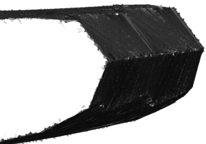
|
| Figure 112: Wing leading edge resolved with distance function - For the representation five refinement steps were applied. |
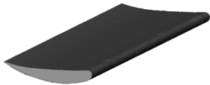
|
|
| (a) Without mesh lines | (b) With mesh lines |
| Figure 113: Result of the distance function applied to a fine wing structure mesh - For the representation five refinement steps were applied. | |
Independent of a specific application example we also want to demonstrate that these refinement strategies are very useful to resolve problems in terms of the approximation of plane and cube edges as discussed in previous sections. The corresponding results are presented in the figures 115 and 116.
At the end of this section we may conclude: Using an embedded method it is generally difficult to approximate edges and very thin structures. In our case, though, powerful strategies could be proposed to handle the corresponding problems. In particular the application of automatic refinement strategies yielded promising results and also appeared to be superior over creating a finer fluid mesh in advance. However, the presented strategies could only reduce the mentioned problems rather than completely overcome them. Furthermore we note that the use of the refinement strategies and their efficiency depend on the specific application. In section 7.1.5 this will be investigated in more detail.
7.1.4 About a more efficient computation of the approximated structure surfaces
As already introduced in chapter 4 two powerful methods exist to efficiently reduce the computation time in an embedded approach: spatial search and parallel computing. In this chapter we want to discuss our implementation of these methods in the given embedded approach as well as evaluate the resulting computational efficiency. This also includes the investigation of an optimal parametrization of the corresponding algorithms in order to speed up the simulation as much as possible. We start with a discussion of the spatial search and then proceed with an evaluation of parallelization techniques applied to the current distance function.
7.1.4.1 Spatial search based on octrees
The necessity of spatial search algorithms was extensively explained in section 4.2. In there we found that the complexity of the spatial searches implemented in our approach are of order rather than the original order of . The corresponding reduction in complexity becomes quite impressive when actually expressing it in numbers. To this end let us assume an FSI setup with a complex structure geometry which needs to be modeled with triangle elements, e.g. a Formula 1 car. In order to get reasonable results from the pure fluid simulation, we assume tetrahedra elements.
Without doing any FSI simulation, the mere search for intersections in the framework of the embedded approach would consist of triangle-tetrahedra pairs which might intersect. This setup was tested and the pure search for intersections could not be finished by a normal desktop computer within one day. Actually, however, this process would be called every iteration of every single time step of a partitioned FSI simulation, which is hence definitely not affordable.
As justified in the theory part, we will use octree search for improving the search for intersections between fluid tetrahedra and structure triangles. The basic procedure for finding the intersections was derived in chapter 7.1.1 and the corresponding algorithmic structure is indicated in the flow chart in figure 53. Generally, this structure can be maintained and it is just extended by an octree search algorithm. The final algorithm then reads as visualized in the flow chart in figure 117.
In the figure, the original steps from the previous flow chart are visualized with a white background whereas the added steps are highlighted in orange. Before looping over all fluid elements the octree is generated around the structural geometry according to the specified refinement level. Each leave of the octree stores pointers to all structural elements which are spatially contained in this cell. In figure 118 such an octree is generated step-wisely based on a sphere geometry. Beginning with one cell - we will define this as an octree of level 0 - the octree is refined in every step according to the given geometry. Up to level 2 there is no significant pattern in the octree as the sphere is small compared to the octree bounding box. At level 3 and the following more and more octree leaves appear around the sphere surface. At level 8 finally one can observe a clear layer of small leave cells around the surface.
Proceeding in the flow chart, in every loop over the tetrahedra we first look for all octree leave cells which have an intersection with the respective tetrahedron. This is done efficiently by a first rough search in which a bounding box is constructed around the tetrahedron and checked with which leave cells this box has an intersection. Therefore we can reduce the more complex algorithm for checking the intersection box-tetrahedra to a simple box-box intersection algorithm. Only after such intersection was found, a fine search follows which checks for an existing box-tetrahedron intersection using the algorithm described in [47]. Based on this evidently reduced subset of structure elements the search for intersections of these elements with any of the six tetrahedron-edges is performed.
Having the octree search implemented, we want to assess its performance and especially gain a valuable conclusion about the most effective adjustment of the octree parameters in the scope of a given FSI setup. In this concern the octree (refinement) level plays a central role since it influences the appearance of the octree around the embedded structure. Therefore we will further investigate how to choose the level of refinement in order to get the best benefit from the octree search. As the octree is constructed around the structure, the respective shape and size will also play an important role. To allow general conclusions we will propose reasonable test cases in the following.
In order to assess the optimal octree level to a given FSI setup we will propose several simple scenarios and test them with many different octree levels. We will keep track of the computation time needed for the distance function, the time for generating the octree and the number of generated octree leaves.
As mentioned above, the size of the structure and by that the hence connected size of the finite elements used for its discretization, might have a significant influence on the necessary octree level. As a first test example we will assume a sphere discretized with different numbers of elements in different orders of magnitude: . We will also consider a cube which just needs 12 triangle elements to be fully described. By that we also have a structure with a very low number of elements. Furthermore it is worthwhile to see whether the complexity of the structure has an influence on the computation time. Hence we will also investigate a model of a Formula 1 car with the same number of elements as the finest sphere mesh ( elements). Finally we will investigate how sensitive the optimal octree level is to the number of elements in the fluid mesh and the computation time in general. A coarse mesh with elements and a fine mesh with elements will be chosen for each of the proposed structure meshes.
First of all we want to examine the octree-related problems which are linked to the generation of the octree leaves. As the octree is being refined with increasing octree level, the number of leaves is increased as well. When using a coarse structure mesh, the octree will just add some hundred or thousand of leave cells with each further refinement. When using a fine structure mesh, a larger magnitude of leave cells is added with each refinement - up to some million cells. In figure 119 the number of structure elements contained in one octree leave with different structure meshes is illustrated in dependence of the octree level.
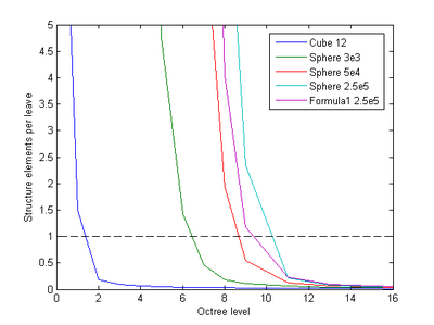
|
| Figure 119: Number of elements per leave depending on octree level - Different structure meshes are used for comparison. |
The figure shows first of all that there is a much larger number of structure elements contained in one octree leave when the octree level is small. This makes sense as an octree leave is then quite big compared to the size of one structure element. There is an exponential behavior when the octree level is increased, especially showing a steep gradient for smaller octree levels. This basically results in a very inefficient use of the spatial search and can be seen in a quite large computation time. Furthermore one can observe a strong difference between the several structure meshes. The more elements are used for the structure the more the curve is shifted to the right as the structure elements are much smaller for fine meshes.
In the figure we have included a dotted line at which one structure element is contained in one octree leave. This is a quite crucial limit as explained in the following. The aim of the method is to reduce the set of elements in a certain spatial domain. If the number of structure elements in a leave is large, the spatial search within one leave is still not optimal. But if there are more leaves than elements, it implies that each element is assigned to several leave cells. That would mean that we would look for this element several times making it again inefficient. Therefore having one structure element per leave might be an optimal adjustment in terms of efficiency. We will see later whether this statement can be verified.
Generating more and more octree leaves obviously comes along with a larger effort to construct the octree and results in a larger amount of data. The influence can be illustrated by means of figure 120 in which the octree generation time in relation to the complete distance computation time is shown depending on the octree level.
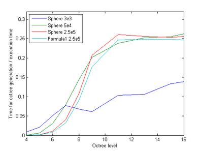
|
| Figure 120: Octree generation time in relation to execution time depending on octree level - Different structure meshes are used for comparison. |
The cube and the coarsest sphere mesh are not visualized as the time for generating the octree can be neglected. But when finer meshes are used, the octree generation time can not be neglected at all. For small octree levels the generation time does not influence the execution time a lot. However, after a certain octree level, it is more or less exploding and the generation can take up to 27 % of the execution time. For a fine sphere for example the octree is generated in less than a second when using a small octree level. But for more than 12 levels it takes already 5 to 15 seconds. This again shows that the octree level can not be increased arbitrarily as the increasing time for generating the octree will diminish the efficiency at a certain point.
Now want to investigate the influence of the octree on the execution time of the distance function. When we were conducting the computations with different octree levels ranging from 0 to 24 it is interesting to note that some setups could not even be computed in an adequate time frame and had to be aborted. For example the sphere with the finest mesh in combination with the fine fluid mesh is computationally so demanding that we had to abort the computation after 12 hours using an octree level of 3. With an octree level of 4 it still took hours to perform the distance computation. Even the coarse sphere mesh with just elements took 4 hours to be analyzed when using an octree level 0 (i.e. not using any octree search). It, however, jut just took some seconds when using a level larger than 4. This again shows the advantages of the octree search.
The figure series 121 summarizes the computation times for each setup whereas the minimal computation time for each setup is marked with a dotted rectangle.
There are several conclusions which can be made from these charts. First, it is obvious that there is always a minimal computation time which depends on the FSI setup. Second, the finer the mesh is chosen the more sensitive the octree level is w.r.t. to modifications. For a very coarse mesh it does not matter which octree level is chosen. For a finer mesh the difference between the optimal and the maximal computation time is getting larger. The finest mesh causes even for a small octree level an explosion in computational costs. Third, the computation time is strongly increasing if the octree level is increased beyond the optimum.
Moreover, when we compare the optimum with each other, it is being shifted towards larger octree levels as the sphere is meshed finer. This also matches to the statement from above that for smaller structure elements the octree leaves have to be decreased. Concerning the influence of the fluid mesh on the optimal computation time we notice that the octree level with minimum computation time is not changing with the level of refinement of the fluid mesh.
A more convenient visualization of the optimal octree level can be obtained when they are collected in one single chart as done in figure 122. This chart depicts the optimal octree level for each of the structure meshes. Here, though, we do not use the number of structure elements but the averaged size of the structure elements as this is a parameter which is comparable between the different structures.
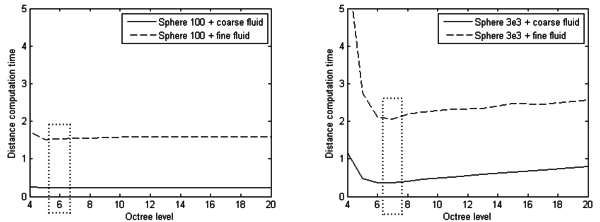
|

|
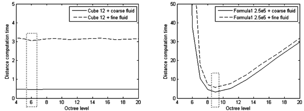
|
| Figure 121: Execution time of distance function depending on octree level - For each FSI setup a chart is presented. The minimal computation time is highlighted by a dotted rectangle. |
Figure 122 also confirms the dependence of the optimal octree level on the size of the structural elements. The finer the structural mesh the larger the octree level has to be chosen in order to minimize the computation time. This correlation can be stated independent of the complexity of the structure, the fluid mesh or the size of the structure itself. Therefore the minimal octree level can be determined only based on the size of the structural elements. The chart hence provides a general decision base for later applications in which we want to choose the octree level according to the structure model in order to get the best possible improvements in computation time.
The figure also shows a straight line which characterizes the setup in which the structural elements have the same size as the smallest octree leaves. All the test cases are quite close to this line which confirms the assumption that the optimal octree level is reached when the leaves have the same size as the structural element. That allows us to directly estimate the optimal number of octree cells for a given structural element size if the size of a structural element is equated with the size of the octree leave :
|
|
(7.31) |
This can be done assuming that the size of the original octree cell is in unit space (1x1x1) which is the case for all computations that have been done in the framework of this monograph.
Finally we conclude that for any chosen configuration of structure and fluid the octree search significantly reduces the computational effort related to the spatial search that is needed in the embedded approach. The improvement is controlled by adjusting the octree level. Its optimal value is depending only on the size of the structural elements.
7.1.4.2 Parallelization with OpenMP
In this section we want to shortly examine the potential of parallel computing with OpenMP applied to the distance function. For the tests the supercomputer CaesarAugusta in Zaragoza, which has 512 processors, was used. However, there are 64 processors in maximum which share the same memory what allows us to use up to 64 processors with OpenMP for the following performance studies.
In order to test the performance of the distance function, it makes sense to test the scalability with different fluid meshes: a coarse mesh ( elements), a finer mesh ( elements) and a very fine mesh ( elements) . As structure we use a sphere with elements. The reason for just varying the fluid mesh can be argued with the way of how it is implemented. When referring to the initial flow chart for embedded methods (figure 4) we will just parallelize the for-loop which performs a loop over all tetrahedra elements and keep the structure unchanged. In order to do that, a function is called which partitions the complete fluid mesh into submeshes whereas is the number of threads which are chosen. Each of the submeshes contains roughly the same number of elements. A big disadvantage of doing this is that there might be many threads assigned to parts of the fluid mesh that do not intersect the structure at all. This can lead to a bad load balancing.
First of all, the computations of the distance function are performed with a varying number of processors. Based on the execution time, the speedup as well as the efficiency can be computed according to the equations presented in section 4.1.3. Finally, the speedup graphs for the different fluid refinements can be plotted in one chart (see figure 123).
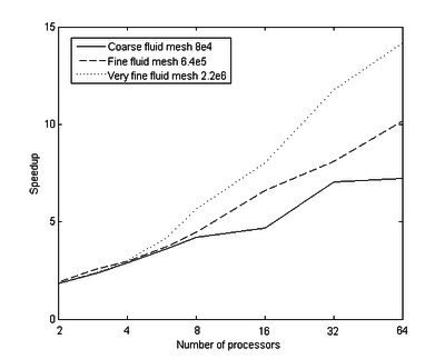
|
| Figure 123: Speedup with OpenMP - The figure indicates the speedup depending on the number of processors for different fluid meshes in a comparison. |
The speedup graphs show a clear reduction of computation time when the number of processors is increased as the computational effort is shared between more and more processors. For all of the three setups (coarse, fine, very fine mesh) the maximum speedup can be reached with 64 processors implying that it is recommended for all following computations to use 64 processors in order to exploit the technique of parallel computing as much as possible. The achieved speedup is almost identical for the different setups when using a smaller number of processors.
A clear distinction can be observed when more than 8 processors are applied to perform the computations. The finer the fluid mesh, the larger is the gradient of the speedup curve. Therefore parallel computing is getting more efficient when a finer mesh is used. The best speedup which could be achieved is 14 meaning that the distance computation can be performed 14 times faster than the execution with just one processor. Therefore the code is said to be scalable.
When having a look at the efficiency plot (figure 124) one can see the reduction of efficiency for increasing number of processors which points to a less utilization or exploitation of the processor performance.
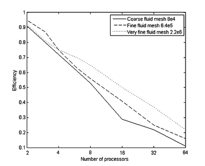
|
| Figure 124: Efficiency with OpenMP - The figure shows the efficiency depending on the number of processors for different fluid meshes in a comparison. |
The finer the mesh the better the processors can be utilized towards capacity as the efficiency is larger for finer meshes. This also explains the higher achievable speedup for fine meshes compared to coarse fluid meshes.
All in all, the parallelization is worth to apply for further computations as it offers a large potential towards a reduced computation time, especially for large and time-consuming simulations. A further improvement of computational efficiency can be reached when the code is also parallelized with MPI such that also more than 64 processors of the supercomputer can be used. Due to this promising potential, the distance function was also provided and tested with MPI. The intrinsic concept of the embedded method to use purely element-wise distance functions turns out to be very advantageous for the application with MPI.
The function principle is illustrated in figure 125. The approach is simply to replicate the structural model on all of the processors, i.e. each processors gets the full model of the structure. Further, each processors has a partition of the fluid model.
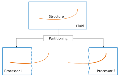
|
| Figure 125: Embedded method parallelized with MPI - The fluid domain is partitioned and assigned to the processors, whereas the structural model is replicated on all of the processors. |
This partitioning was already explained in chapter 4.1.4; the flow chart in figure 28 shows the algorithmic structure. Since the distance computation is purely local on the elements, it can be performed on every CPU separately without any communication with the other processors.
Unfortunately it was not possible to do any studies in terms of the speedup and efficiency which can be reached with MPI because the access to the supercomputer was not available in this phase. However we expect the speedup to be even larger than with OpenMP.
7.1.5 Performance of the embedded method in large-scale examples
In the previous chapters we have extensively discussed and step-wisely improved the performance of the distance function by means of chosen test cases which exhibit a certain common geometrical characteristic. Also, different refinement strategies were proposed in case the distance function is not able anymore to describe the smallest structural details. In this chapter now, all those ideas are applied to practical large-scale examples. One goal of this chapter is to demonstrate the performance and capabilities of the current distance function applied to arbitrarily complex geometries. This will on the one side provide a decision base for users of the method to chose the optimal setup for a given FSI configuration but will also one the other side show clearly the limits of the method. To this end, we will in the following test the distance function with a model of a Formula 1 car, a hangar and a 3-sails model.
7.1.5.1 Geometric approximation of a Formula 1 car
The first large-scale example is the Formula 1 car. The surface mesh of the structural model is shown in figure 126. It is composed of triangle elements in order to resolve all the geometrical details properly. Note in this context again that the distance function can just be as accurate as the structural mesh represents the original structure.
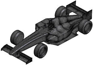
|
| Figure 126: Structure mesh of Formula 1 car - The surface model is meshed with triangle elements. |
The application of the distance algorithm to such complex models with many small-scale details is a challenge. Hence we want to test several refinement strategies and see which of them is the most effective and which achieves the best approximation of the structure. As already discussed in section 7.1.3 one way to encounter such a complex geometry would be to refine all the split elements with the thought in mind that the model will end up with a large number of elements. Nevertheless this strategy might be efficient when applied to this model as it does not show many large-scale planar or slightly curved surfaces. There are a lot of geometrical details as the aerodynamic elements which are composed of many thin structures and sharp edges or the side pots which exhibit surfaces with large curvature.
Refinement strategy 1
As an initial setup we will choose a coarse fluid mesh ( elements) and apply 4 refinement steps in a row whereas in each of them all split elements are refined. Figure 127 illustrates the situation. A first look at the fluid mesh shows that the refinement strategy performs a regular refinement of all elements along the structure.
After four refinement steps the size of the fluid elements close to the structure is very small compared to the surrounding elements which are not split. One can even observe a kind of a gradation of the element size when approaching the structure which could be interpreted as a step-wise reduction of the element-size towards the structure surface. As an outlook one might investigate the potential of this gradation to be used as a boundary layer mesh for simulations of boundary layer separation. The achieved approximation of the structure is indicated in figure 128.
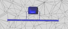
|
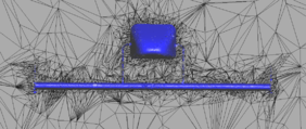
|
| (a) No refinement step | (b) 4 refinement steps |
| Figure 127: Comparison of fluid meshes with refinement strategy 1 - The fluid meshes are cut at the front wing of the Formula 1 car (blue). | |
Without using any refinement one can just guess that a car shall be represented. The structure approximating elements are quite large and can not resolve the small details of the car. Already after two refinement steps, the overall structure is resolved approximately and after four levels the car body seems to be represented in a high accuracy and can be well compared to the original structure model. However, some deficits become first visible when having a closer look to the front wing (figure 128d).
Although the wing is approximated with an acceptable accuracy, it is not possible to resolve the wing tip edges or the connecting element of the wing to the car body. Moreover, many elements are used to represent the front car body which is generally planar. A refinement at such large-scale surfaces is actually not necessary. Besides, the figure shows clearly the regular size of the structure-approximated mesh which originates from the refinement strategy.
Refinement strategy 2
Due to the mentioned drawbacks we want to propose another strategy which just concentrates on refining those elements that can not represent the structure with an acceptable accuracy. That was already discussed at the end of section 7.1.3. The aim we follow with this strategy is on the one hand to directly approach the structure details which are hard to detect and on the other hand leave the elements unchanged which cut planar or slightly-curved structure surfaces. We expect the aerodynamic elements to be resolved much better.
As a first step we want to have a look at the fluid mesh cut at the front wing (shown in figure 129) after five refinement steps.
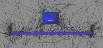
|
| Figure 129: Fluid mesh with refinement strategy 2 after 5 refinement steps - The fluid mesh is cut at the front wing of the Formula 1 car (blue). |
At first glance one can observe the extremely refined fluid elements close to the thin end-plates left and right. Here they are much more refined compared to those around the main wing surface. Also at three corners of the car body the fluid elements are significantly refined. A comparison to strategy 1 (see figure 127b) illustrates the different approaches. The achieved representation of the structure is shown in figure 130.
The approximation without using any refinement is not presented here as it is exactly the same as shown in figure 128a. The potential of the applied strategy becomes obvious when more than two refinement steps are used (figure 130). The car body at the front for example is represented with mainly large elements since it is composed of large planar or slightly curved surfaces. The strong curved spots as the sidepod curvatures are resolved in detail and represented by means of many small elements. Especially the front wing exhibits many tiny elements as is indicated in figure 130d. Compared to the front wing resolution of the previous strategy we could improve the representation a lot particularly at the sharp edges.
Although the details are resolved in a very promising manner one might want to resolve the car body or particularly the tires better. A closer look to the tyres would reveal a quite edged representation of the tyre. In order to resolve also those surfaces better, a much finer fluid mesh can be chosen. In the following strategy a mesh with elements is applied and the same refinement strategy is being used.
Refinement strategy 3
Applying a finer fluid mesh at the beginning results in a better structure representation already without using any refinement as figure 131 clearly indicates.
Moreover it is sufficient to just use four refinement steps in order to get similar results as with the previous strategy in which a coarser mesh was applied. But the main difference is that the large-scale surfaces and the curved tires are resolved much better. Of course, this will lead to more fluid elements but this step is essential to get a well-defined structure. After the fourth refinement step the fluid model exhibits elements whereas the coarser fluid after the fifth refinement step (strategy 2) exhibits just elements resulting in a considerable additional computational cost. But there is an alternative way to encounter this computational overload if we just consider again the deficit we had to face when applying strategy 2. After five refinement steps the structural details are well resolved but the tires could be approximated much better. To overcome this problem we can replace the last refinement steps by one step performed with strategy 1 in which all split elements are refined. This results in a combined strategy and will be discussed in the following.
Refinement strategy 4
Here we will use the coarse mesh and apply three refinement steps with strategy 2 followed by one step with strategy 1. The direct comparison of this strategy compared to the pure application of strategy 2 is shown in figure 132.
In the lower two figures one can directly see the impact of the last refinement step on the structure representation. The comparably large elements throughout the car body and the tires are noticeable refined which influences the accuracy of the overall structure. This turns out to work very well for the given structure, but there is no definite strategy which is the best strategy as it depends on several parameters. The assessment of the accuracy of the approximation of the car was just based on a visual evaluation and is hence very subjective. Quantitative measures to assess the quality of the approximation are missing here. Therefore we aim at proposing efficient strategies in order to demonstrate how the results can be modified by choosing a different approach of refinement and adapt the result according to the technical requirements.
Hence it is more a balanced combination of the presented strategies which leads to a promising result. The fineness of the large-scale planar or slightly-curved surfaces can be adjusted by means of the first proposed strategy whereas the fine details of the structure can only be captured with refinement steps performed with strategy 2. Based on this experience we will demonstrate the geometrically best result we could achieve with the given computational power in the following strategy.
Refinement strategy 5
This strategy is a mixture of all up to now applied strategies. First of all, the fluid mesh is entirely refined to elements. Then, four refinement levels with strategy 2 are performed followed by one step with strategy 1 in order to resolve the large-scale surfaces. By that, we will end up in an exceptionally accurate structure model as illustrated in figure 133.
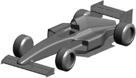
|
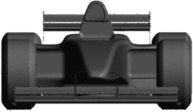
|
| (a) Isometric view | (b) Front view |
| Figure 133: Approximated structure with refinement strategy 5 - A combination of all previously presented strategies was used to get this final result. | |
It should be mentioned that the fluid mesh after the last refinement step is composed of elements which is a considerably large number of elements and is only affordable with powerful supercomputers. Nevertheless we find that such structures are not suitable to be used with the embedded method due to the discussed reasons. The ALE approach would be much more efficient in this case.
Having a closer look to the undertray reveals the already before observed “holes” in the structure as shown in figure 134. Such discontinuities have already been discussed previously in the section dedicated to thin structures. As this irregularity in the geometry arises here again, we want to investigate such structures more precisely in order to prove that the fluid can not cross the thin plate although it appears to allow this. This will be done in the subsequent chapter.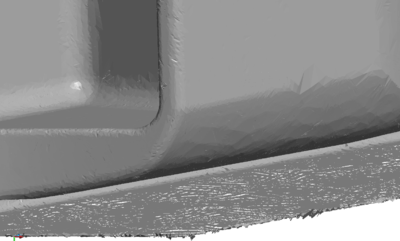
|
| Figure 134: Undertray of Formula 1 car - The small white spots indicate slight geometrical discontinuities. |
7.1.5.2 Geometric approximation of an inflatable hangar
The hangar model was already mentioned in the introduction in chapter 1. Here we will consider just a part of the full hangar model which is composed of four connected tubes as visualized in figure 135.
The level of detail of the structure model is much lower compared to the previous model, as we e.g. do not encounter problematic thin structures. However, the glue seams between the tubes as well as the transition of the tubes to the base plate turn out to be challenging for the distance function. That implies to use some initial refinement steps applied in strategy 2. Furthermore the model exhibits large-scale surfaces with a curvature which is not negligibly small. Therefore we will first choose a rather fine fluid mesh ( elements) as starting point.
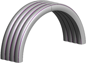
|
| Figure 135: Hangar model (CAD) - The model is composed of four curved tubes. |
In order to represent such curvature accurately we want to use an additional refinement step with strategy 1 (refine all split elements). This will resolve the curved tubes more precisely. Based on this assessment, the following refinement strategy will be chosen:
- Generate fine fluid mesh: elements
- Refinement strategy 2: 3 steps
- Refinement strategy 1: 1 step
Applying this strategy to the fine-meshed structure ( elements) yields the approximation shown in figure 136. Already without any refinement, the shape of the tubes can be roughly captured (figure 136a). The curvature and the sharp edges at the base, however, can not be represented accurately. After the first three refinement steps (figure 136c) the hangar approximation converges very well to the original model. Solely the surface of the tube exhibits some edged indentations which can be smoothed by applying strategy 1 again as shown in figure 136c. The precise representation of the sharp edges at the base is shown in figure 136d.
7.1.5.3 Geometric approximation of sails
Finally we also want to consider a one-sided membrane structure composed of three sails which are part of a sailing boat as visualized in figure 137. With regard to the complexity of the structure one can state that the level of detail is even lower compared to the hangar model. Two of the sails have comparatively planar surfaces whereas the third sail has a slightly curved surface. All sails feature a sharp edge along the sails boundary which turns out to be the only challenge to handle. As one could expect, the large-scale surfaces of the sails can be approximated very accurately with a rather fine fluid mesh ( elements). Therefore we will reduce the strategy to just concentrate to the proper representation of the sails edges. That implies the mere use of strategy 2. The result of this refinement strategy after applying it four times is shown in figure 138.

|
| Figure 137: Sails model (CAD) - The structure is composed of three membrane sails. |
As expected, the sails' surface can be precisely approximated by means of the rather coarse fluid mesh without application of any refinement. After four refinement steps the surface can be even more resolved. The strategy turns out to be efficient as the edges can be clearly represented. After the last refinement, the fluid is finally composed of elements.
At the end of this chapter we may summarize: We have shown how arbitrarily complex shaped geometries can be approximated by using various powerful refinement strategies. As pointed out there is, however, not one single strategy which can always be applied to get the best results. The user rather has to first assess the complexity and level of detail and check it towards the required aims concerning the final application in FSI. Based on this an optimal strategy can be developed. However, the user should keep in mind, that those refinement strategies increase the number of degrees of freedom immensely yielding an additional computational effort that can not be neglected. Moreover it should be emphasized that these strategies do not eliminate the inaccurate representation of sharp edges but rather reduced the corresponding approximation error.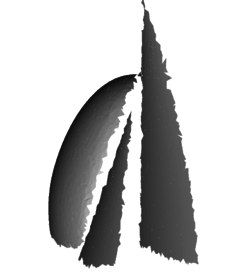
|

|
| (a) No refinement step | (b) 4 refinement steps |
| Figure 138: Proposed refinement strategy applied to the sails model - The approximation is achieved by applying strategy 2 four times. | |
7.2 Influence of the interface treatment on the flow field
In the previous chapter an algorithm to compute the distance function for arbitrarily shaped embedded structures was developed. However, some limitations were pointed out which result in an increasing approximation error that probably affects the later FSI simulations. In this context we want to investigate in the following the influence of the geometric representation on the flow field, which can be thought of as a "snapshot" of a certain time step during an FSI simulation. In the first part we discuss a problem that refers to the discontinuous flow across a very thin plate. The objective is to prove that - despite of the local reduction of a two-sided structure to a one-sided surface - the "flow border" of the plate is still maintained. In the second part then, we want to qualitatively and quantitatively assess the performance of the distance algorithm by means of the well-known Silsoe benchmark.
7.2.1 About the discontinuous flow across a thin plate
In sections 7.1.3 and 7.1.5 we already figured out that very thin structures such as the front wing or the undertray of the given Formula 1 car lead to difficulties w.r.t. a proper approximation. These difficulties are caused by the inability of the finite fluid elements to represent both sides of the thin structure by a set of distance values. The proposed remedy was to locally collapse the thin structure to one single surface.
By doing this, however, strong geometrical discontinuities are generated which are seen as small holes in the post-processing (refer to figures 106 and 134). In order to eliminate the possible misunderstanding that the fluid might flow across the structure through these holes we want to demonstrate in a computational experiment that the flow border is still maintained. This proof would also support the physical correctness of the above-mentioned method in which the two-sided structure is locally reduced to a one-sided structure.
Therefore it is appropriate to assume a very thin plate which is fixed within a fluid channel. The proposed setup is illustrated in figure 139. The thickness of the plate is just a hundredth of the smallest width such that we can ensure that the fluid can not properly resolve the plate and hence provoke the mentioned problem case. The fluid is flowing within a channel whereas the prescribed velocity profile at the inlet is a prescribed parabolic, i.e. analytic, profile in order to simulate a real channel flow. The peak velocity of the profile is defined to be . Furthermore, water is chosen as fluid. As a result a laminar flow will be computed.
In a first step the plate surface will be approximated by refinement such that the representation does not show any one-sided elements. This serves as a reference simulation to which we can compare the simulation with a visually “porous” structure in a second step. With regard to the refinement strategy it is enough to refine only such elements which exhibit double-cut edges. This refinement is performed four times, leading to the result shown in figure 140.
The approximation shows a well-defined surface without any one-sided elements. Based on this, the fluid simulation is performed. The fundamental theory and implementations connected to the embedded solver can be taken from the theory part in chapter 2.2.4 and will be further discussed in chapter 8.1. Here we do not want to go into detail and therefore leave out any discussion concerning the solution procedure. The achieved results of the velocity field are shown in figure 141. The figure shows exactly the expected discontinuity of the velocity field in flow direction across the plate. Due to better visibility the negative values have been left out in the visualization. Such flow behavior is what we also expect from an embedded plate that is not well resolved.

|
| Figure 140: Approximation of the plate with four refinements - This structure does not contain any one-sided elements. |
Based on this we want to see how the flow behaves if we do not apply any refinement strategies. In this test case the approximated plate exhibits many one-sided elements as the skewed view of the plate in figure 142 shows quite impressively. In the upper figure the mentioned voids are clearly visible. Also the lower figure illustrates in a skew view of a cut across the plate that there are elements in between the two sides of the plate which results from a local reduction of the two-sided structure to a one-sided. Based on this approximation we want to investigate how the flow behaves and whether the discontinuity of the flow across the plate is still maintained. The results of the simulation are shown in figure 143.
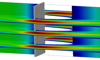
|
| Figure 141: Velocity field in x-direction with the well-resolved plate - In order to be able to see the discontinuity of the velocity field the negative values are ignored. |

| |
| (a) Side view | |
| |
| (b) Skew view of a plate cross section | |
| Figure 142: Approximation of the plate without refinement strategy - The structure contains many one-sided elements. | |
At a first glance, the discontinuity does not seem to be fulfilled throughout the entire plate. Particularly at the edges of the plate there is fluid flowing across the plate indicated by the positive velocity field directly behind the plate. This can be explained by the fact that the region around the side walls of the plate is difficult to represent as within a small domain three surfaces with completely different orientations (the side wall and the two main large-scale surfaces) meet. This results in a intersection pattern which combines rectangular corners (e.g. as seen with the cube) and thin structures (as seen with the wing), which are based on different strategies. That leads to an irregular representation of the structure including elements which are skew-aligned towards the flow direction. The consequence is that the flow is locally changing its direction at the edges.
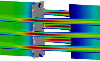
|
| Figure 143: Velocity field in x-direction with the badly resolved plate - In order to be able to see the discontinuity of the velocity field the negative values are ignored. |
However, we want to focus on the flow in the mid-section of the plate. In this area, we can not realize any velocity component in flow direction. If the structure voids allowed the fluid to pass, this would happen at many locations throughout the plate leading to a visible velocity component at those spots. It is important in this context to not misunderstand the small colorful spots which can be detected at a few locations. They originate from the fact that one can look through the porous structure approximation and see the flow field behind the plate.
All in all we have visually proven that the approximation of thin structures with the applied method is physically reasonable and allows to provide the required flow discontinuity.
7.2.2 Silsoe benchmark: A comparison of CFD solutions from a body-fitted and an embedded analysis
Up to now the investigations just allowed a qualitative assessment of the performance of the developed distance function. With regard to FSI simulations that follow in the subsequent chapter it is also necessary to perform a quantitative assessment of the flow field around an approximated body. The performance evaluation can be supported by a direct comparison to a flow field around a perfectly resolved body surface. A very common benchmark for the validation of CFD codes is the Silsoe benchmark which is based on experimental data of a wind flow around a huge cube. In this chapter we will refer to the corresponding paper of Richards [54]. Many tests have been performed in the years before in order to collect data about the pressure and velocity field in the region around the cube.
The Silsoe benchmark was already analyzed extensively by Gerhard Steber [39]. He profoundly compared CFD solutions with Kratos based on a body-fitted mesh to the experimental results of the Silsoe benchmark. This provides an ideal reference to compare our results obtained with the embedded method. Referring to his simulation results gives us the opportunity to assess the performance of the embedded solver qualitatively and quantitatively. In this chapter, we will consider the Silsoe benchmark once with the use of a slip condition at the cut elements and once with a no-slip condition, whose formulation is supposed to better represent the experimental results. Gerhard Steber used exclusively no-slip conditions. It should be noted here, that the simulations based on a no-slip condition were conducted at the end of the herein described project phase. Thus, we will present only first results. Due to the intensive research work which is currently in progress, the applied approach will be illuminated in detail in subsequent papers.
Setup of the Silsoe benchmark
The Silsoe benchmark focuses on a wind flow around a cube with an edge length of 6 m. The wind direction is chosen such that the wind impinges perpendicular to the cube surface. In order to be able to compare the final results to Steber [39], we will choose the same setup of the Silsoe and also the same mesh sizes for the fluid domain later on. The dimensions and boundary conditions are illustrated in figure 144.
The inlet velocity is modeled as logarithmic profile in order to simulate a real ground flow. At the opposite surface an outlet pressure of zero is imposed to control the flow direction. Along the side and top walls a slip-condition and on the ground a no-slip condition is imposed. In a first simulation, slip conditions are applied to the cube surfaces as opposed to the model of Steber. This implies that the description of the wall-near shear-stresses influencing the velocity field is not possible. The embedded solver by construction allows to weakly impose slip-conditions to the boundary as the modified shape functions are defined to not permit any variation of velocity and pressure in direction to the interface within a single element (discussed more in detail in chapter 2.2.4.2). In a second simulation, no-slip conditions (application of a wall-law) are imposed to the cube surfaces, which reflect the setup of Steber. In chapter 2.2.4.3 the definition of a wall-law for the embedded approach is proposed by introducing a pseudo viscosity and therefore generate an artificial stick boundary condition.
In order to compare the results from the simulation to the pressure of a full scale model with different density the mean pressure coefficient is introduced. By means of that coefficient the pressure is scaled to a generally comparable dimensionless number:
|
|
(7.32) |
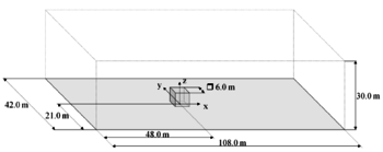
| |
| (a) Dimensions | |
![Setup of Silsoe cube - The figure indicates the dimensions and boundary conditions for the Silsoe benchmark (Source: Steber [39]).](/wd/images/thumb/e/ee/Draft_Samper_908356597-monograph-J01_SetupFluidBC.png/350px-Draft_Samper_908356597-monograph-J01_SetupFluidBC.png)
| |
| (b Boundary conditions | |
| Figure 144: Setup of Silsoe cube - The figure indicates the dimensions and boundary conditions for the Silsoe benchmark (Source: Steber [39]). | |
Here, is the pressure which is supposed to be evaluated, , and are freestream parameters which are measured far away from the turbulent zone. As proposed in the paper of Steber, we will evaluate the freestream parameters at the point (-23,4 m; 6,24 m; 6,0 m). The simulation is also run over a period of 80 s and the record of pressure and velocity parameters is started after 30 s, when the flow is developed through the entire domain.
In order to directly compare the results to Steber, it is necessary to use the same evaluation points along the cube as he used in his paper and which were also initially proposed by Richards [54]. The following figure 145 indicates the three evaluation planes at , and along which the pressure field is captured.
![Evaluation planes of pressure field - Three cutting planes define the evaluation lines on the surfaces of the cube along which the pressure is recorded (adapted from [39]).](/wd/images/thumb/2/2d/Draft_Samper_908356597-monograph-J02_EvaluationPlanesPressure.png/200px-Draft_Samper_908356597-monograph-J02_EvaluationPlanesPressure.png)
|
| Figure 145: Evaluation planes of pressure field - Three cutting planes define the evaluation lines on the surfaces of the cube along which the pressure is recorded (adapted from [39]). |
Procedure of the simulation
The simulation with the embedded approach requires many additional steps compared to the CFD simulation with a body-fitted mesh. The procedure of setting up the model and the embedded solver as well as the solution and the evaluation is visualized in the flow chart in figure 146.
In there, the completely prepared fluid as well as the structure mesh are loaded at the beginning of the simulation and the steps for initializing the variables, solvers and input/output are performed. Based on both meshes, the distance function is applied. Therefore one has to note the circumstance that the distance function does currently just work in unit space as the initial octree cell is generated with the dimensions (1;1;1). Thus it is required to scale both models uniquely down to the domain with the box bounded by the origin and the point (1;1;1). Within this normalized space, the distances are computed and afterwards the models are scaled back to its original dimension. The underlying scaling equations are the same for both models, whereas the coordinates of each node are modified as follows:
|
|
(7.33.a) |
|
|
(7.33.b) |
|
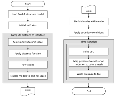
|
| Figure 146: Flow chart for simulation of Silsoe benchmark - The main steps for setting up the models and the embedded solver, the solution procedure and the evaluation of the pressure are listed. |
The equations imply that the fluid box is shifted to the origin such that all nodes of the domain have positive coordinates and afterwards the three components are scaled by the same factor (linear transformation). Subsequently, the elemental distance values are computed. Then, we need to call an automatic inside/outside function to identify which nodes of the fluid mesh are enclosed by the closed structure domain, i.e. the cube volume. This is done according to the in chapter 2.2.4.1 explained technique of ray tracing. All those fluid nodes within the structure (having a negative distance value) can thereby be deactivated and later constrained accordingly.
After rescaling the model, the boundary conditions are imposed to the model and the fluid nodes enclosed by the cube surfaces are fixed in velocity and pressure. Afterwards, the simulation can be started by iterating over time whereas in each step the embedded solver is called. Furthermore, the pressure has to be mapped onto the evaluation points on the cube faces as indicated in figure 145 and the pressure values are written to a file such that the evaluation can be done afterwards. The parameters for the simulations are listed in the following:
Solver settings:
Solver type : Fractional step
Linear solver for velocity and pressure : AMGCL
Solver tolerance :
Convergence criteria settings:
velocity :
pressure :
Problem settings:
Time step = 0.05 s
Simulation time = 80 s
Fluid and structure mesh
The mesh sizes for the fluid are chosen equally to the ones proposed by Steber. He advised to divide the fluid domain into several smaller boxes with each a different mesh fineness (shown in figure 147) as a compromise between a low computational effort but a high accuracy of the pressure and velocity field.
![Discretization of the fluid domain - The volume and surface mesh sizes for the separate cubes are shown (Source: Steber [39]).](/wd/images/thumb/9/9f/Draft_Samper_908356597-monograph-J04_SetupFluidMeshSize.png/500px-Draft_Samper_908356597-monograph-J04_SetupFluidMeshSize.png)
|
| Figure 147: Discretization of the fluid domain - The volume and surface mesh sizes for the separate cubes are shown (Source: Steber [39]). |
It is important to note that - compared to a body-fitted mesh - the domain which is occupied by the cube is also meshed with fluid elements. That will finally lead to a mesh with elements. A cut through the mesh is depicted in figure 148.

|
| Figure 148: Cutting planes of fluid mesh at - The fluid mesh is much finer close to the region around the cube. |
The region around the cube has a much finer mesh than the outer domain in order to better resolve the flow details close to the cube. The structure of the cube can be basically modeled with twelve triangle elements, but in terms of the evaluation of the pressure directly on the cube surfaces the pressure has to be mapped to the prescribed evaluation points. Thus the structure mesh is prepared accordingly whereas the evaluation lines are modeled by a structured line mesh (figure 149). The pressure of the fluid is mapped to the structure by means of an arithmetic averaging as explained later in chapter 8.3.1.
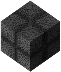
|
| Figure 149: Discretization of the structure domain - Clearly visible is the structured grid along the evaluation lines around the cube. |
The approximation of the cube as a result of the distance function applied to the fine fluid mesh is illustrated in figure 150.

|
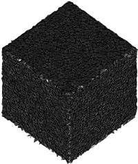
|
| (a) Without mesh edges | (b) With mesh edges |
| Figure 150: Approximation of the cube based on distance function - This is the result without application of any refinement strategies. | |
Evaluation of the results
In the course of this section, the results of the Silsoe benchmark without (slip-condition) and with wall-law (no-slip condition) on the cut elements are analyzed and finally compared to the results gained with the ALE-based simulations.
In figure 151 the pressure fields of the simulation with slip and no-slip condition are directly set in relation to each other. The visualization in terms of isolines was chosen in order to point out the small-scale details of the flow. Also the shapes of the vortices can be captured much better. In a rough analysis of the flow characteristics in both simulations, one can observe the main features of a flow around a bluff body. The flow approaching the cube is stagnating at the front face forming a stagnation pressure zone. Due to the implied large local pressure gradient in combination with the shear stresses at the ground (no-slip condition), a ground-near horseshoe-vortex is formed which can be better seen in later figures. At the upper left edge of the cube the flow is separated and accelerated leading to high turbulence and the generation of vortices above and behind the cube. All in all, the main features of the flow around the cube can be captured with the application of the embedded method.
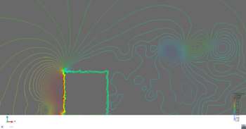
|
| (a) Slip condition |
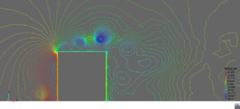
|
| (b) No-slip condition |
| Figure 151: Comparison of pressure distribution with slip condition (a) and no-slip condition (b) at the cube () |
When comparing the pressure field of both simulations qualitatively with each other there is a distinguishing feature which can be traced back to the physical dissimilarity of the conditions. Directly behind the flow-separation edge there are small turbulence vortices when using a wall-law at the cube hull. These are physically correct and also reflect the pressure fields which are illustrated in the paper of Steber. However, these physically reasonable vortices can not be observed when a slip condition is imposed. Due to the missing effect of the near-wall shear stress at the cube, the turbulences after flow-separation are not amplified as it should be the case. Thus, the first vortices start to form far behind the flow-separation edge. This leads to the conclusion that the correct capturing of the flow close to the cube requires the presence of a no-slip condition. Similar observations can be made in a different view of the results as shown in figure 152. We will see later the consequence of a missing no-slip condition in a quantitative comparison.
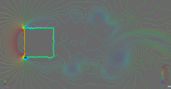
|
| (a) Slip condition |
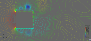
|
| (b) No-slip condition |
| Figure 152: Comparison of pressure distribution with slip condition (a) and no-slip condition (b) at the cube () |
Also striking, when having a closer look at figure 152a, is the zig-zagging pressure profile along the cube surface. This can be explained by a misleading interpolation during the visualization process which is, however, corrected in the second simulation.
Aiming for a quantitative analysis the mean pressure coefficient evaluated along the cube, as indicated in figure 145, is shown in the diagrams in figure 153.
Regarding the first diagram 153a it is evident that the presence of a wall-law at the cube has a massive influence on the pressure field behind the separation edge. This is especially shown by this diagram as it comprises the region behind the separation edge. The embedded approach with wall-law is better reflecting the results of the body-fitted CFD, and especially nearly coincides at positions and . However, there remains a certain deviation with regard to the body-fitted CFD solution. This can be led back to the inaccuracy in geometric representation with the formulation of the embedded method. In contrast, the embedded approach without wall-law is far from being accurate at any position of the cut. Also there is an eye-catching jump in the profile which points to a certain instability. This instability is not observed in the other simulation as such wall-near velocity peaks are avoided by the wall-law.
In the second diagram 153b the pressure distribution in flow direction is shown. The first part between 0 and 1 represents the stagnation zone in which the results of the embedded approach correspond best to the results gained by the body-fitted CFD. However, the embedded method without wall-law shows a large deviation close to the horse-shoe vortex at position . Also at the separation edge (position ) and beyond, the embedded approach with wall-law shows a better coincidence with the CFD based on a body-fitted mesh. The aforementioned observation of the small vortices directly behind the separation edge do in fact reflect in a better quantitative representation of the pressure field. Nevertheless, the embedded method in general struggles with correctly representing the pressure field behind the separation edge.
In the last diagram 153c the stagnation zone at the front of the cube is well-resolved as we could also prove it within the previous diagram at position . At the side walls and behind the cube the pressure coefficient in both cases - with and without wall-law - is differing a lot from the results based on a body-fitted mesh.
Although there are obvious deviations between the embedded approach and the results gained with a body-fitted mesh, it could be shown that the main features can be captured qualitatively with the embedded method. The presence of a wall-law is indispensable to get physically reasonable results, especially behind the flow-separation edges, as small vortices are generated along the side and top walls of the cube. The quantitative comparison revealed a good performance of the embedded approach in front of the cube, but larger deviations arise in the zone behind the separation edge where the flow starts to get turbulent. This might be led back to the problem of a rather rough geometric representation of the embedded cube edges which can never be exactly described by the distance algorithm. However, for future projects it might be an idea to investigate the results of the Silsoe benchmark when using a finer fluid mesh and/or applying appropriate local refinement strategies. This step requires an extremely long simulation time which is the main reason why it was not possible to test it in the scope of this study.
8 Solution procedures for FSI problems
Now that we know how the interface or the geometry is tracked in case of the embedded approach and we got a feeling for how this affects the single field solution quality, we want to proceed to the actual solution procedure with FSI-simulations based on the new embedded and the already given body-fitted or ALE approach. The detailed elaboration, mutual comparison and critical discussion of both of the two different solution procedures is going to be topic of this chapter. Focus here will be the new embedded technology.
The chapter is organized according to the single steps that subsequently have to be introduced in both solution procedures to finally form and run a fully coupled FSI simulation. That is, we will start with a fixed structure in a CFD context and first test the actual functionality and implementation of some of the solution steps within the new embedded solution procedure. Afterwards we will introduce a movement of the structure, i.e. a one way coupling, and hence investigate how differently complex movements are treated in the different approaches. To this end we will develop and elaborate several mesh-updating strategies and compare their performance with the possibilities in an embedded approach. Then it will be discussed how specifically in the embedded case the solution quantities are exchanged. In this context several mapping techniques will be developed and evaluated. Finally, having investigated the handling of movements and the exchange of data, two fully coupled test examples will be simulated using both approaches. This eventually will allow to critically contrast the two methods with respect to their advantages and drawbacks.
8.1 Channel flow with fixed embedded structure
The most simple case of a “fluid-structure-interaction” is the one where the structure is considered to be rigid, i.e. where the FSI-simulation reduces to a single CFD-analysis. In this scenario the structure is embedded in the fluid and remains positioned without inducing state changes to the fluid, as it was e.g. the case with the Silsoe-cube in chapter 7.2.2. In this case and under the assumption of a steady state flow scenario, a correct solution approach implies convergence to a steady state solution. A first possible test to verify the correct implementation and functionality of different solution procedures may thus be a check of convergence under the aforementioned conditions. For the body-fitted approach a lot of corresponding benchmarking was already carried prior to the work of this monograph so without proof we assume a significant simulation procedure in this case. For the embedded strategy, though, the correct implementation and functionality still needs to be verified. First tests to this end will be topic of this section.
With the embedded strategy we already assumed a proper implementation in the above mentioned example of the bluff, voluminous Silsoe-cube. In there, however, we were only interested in the influence of the boundary representation on the fluid results and presumed a correct functionality even though we did not explicitly test the latter. In the following we want to catch that up and verify the functionality for the two main classes of structures that may appear: voluminous structures and infinitesimally thin ones. In particular of interest here is a proper physical representation of the pressure and velocity discontinuities as well as a correct implementation of the ray tracing technique and the slip boundary conditions. The latter characteristics are to be tested and verified in the following by means of two generic examples. Both of these examples are modelled in 3D, however simplified in a sense that we are taking a well known 2D setup and “extrude” it to the third dimension. This will facilitate the analysis of the essential results while keeping the conclusion still valid for the 3D case. Both these examples can be used to discuss various different aspects in terms of the underlying characteristics of each method which is why we also will make us of them in the subsequent chapters.
The first example is a simple laminar channel flow problem in which a rigid membrane is placed at the front end, right behind the inlet with a fixed constant velocity profile. In the scope of this section we will use this example for testing a proper representation of the discontinuities when applying the newly implemented embedded method. The model details are given for two different Reynolds numbers in figure 154. As indicated we are here in a first step neglecting a coupling. So what one would expect from the physics of the model is a steady-state-flow in case of the very low Reynolds number and the formation of vortices for the configuration with a comparatively high Reynolds number. Given the former case, the results from an embedded simulation are compared to a a body-fitted reference solution in figure 155.
As can bee seen from figure 155 the structure is correctly placed by the algorithm and the discontinuities are properly captured with stagnation pressure on inflow side and low pressure on side of the outflow with a distinct terminator in between. So a laminar, steady-state fluid flow in fact forms out. Comparing it to the body-fitted approach there are only slight differences in the solution. In fact these differences are mostly arising due to the different discretizations in both cases. Where we have a very easy mesh configuration in the embedded case, more effort has to be spend to model the body-fitted pendant since here the interface has explicitly to be taken into account as it is obvious when looking at the actual meshing depicted in figure 156. Already for this simple example one of the biggest advantages of the embedded method becomes clear - the advantage of a significantly simpler modeling of the fluid domain compared to a costly modeling in the body-fitted or ALE case.
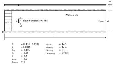
|
| Figure 154: Channel flow with embedded membrane - Note that depending on the test case two different parametrizations are given (low and high Reynolds number). |
In a next step we want to verify firstly a correct distinction of the fluid domain in regions that lie inside the structure and those that are outside. As already explained earlier, a ray tracing technique is used to this end. Secondly we want to verify a correct imposition of the boundary conditions. A correct implementation of these features now can be tested using a second example which is also a channel flow with fixed embedded structure. Instead of the 2D membrane structure, however, we use a bluff, voluminous body with round perimeter, i.e. a rigid cylinder embedded inside the fluid domain. Figure 157 shows the corresponding setup. Different from the example above we are here only using one set of parameters leading to a very low Reynolds number in the laminar regime.
At first it is of interest whether the algorithm correctly distinguishes between inside and outside the fluid domain. In the latter case the pressure and velocity will be set to zero. As can be seen from the results in figure 158 this is in fact done correctly again resulting in a clear terminator between structure and fluid. Without giving more examples it is to be stated that this also works for more complex spatial structures. So the ray tracing can be regarded as verified.
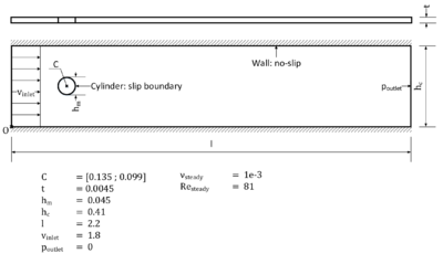
|
| Figure 157: Cylinder embedded in a fluid flow - Note that there is only one set of parameters. |
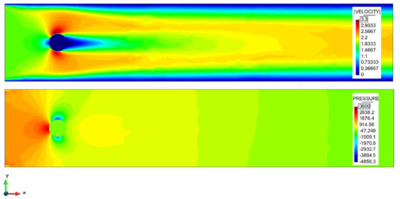
|
| Figure 158: Resulting flow field for the embedded voluminous cylinder from figure 157 after - The depicted results allow to verify a correct ray tracing algorithm as well as a correct imposition of the implemented slip-boundary conditions. |
Having tested a correct identification of the two different domains (outside and inside the fluid), we can check a proper imposition of the boundary conditions. For reasons that were explained earlier in chapter 2.2 it is so far just possible to apply slip-boundary conditions to the embedded interface. Whether these are imposed correctly can be tested easily at the example of the cylinder in the channel flow. Consider the case where no-slip conditions are applied to the cylinder. In this case the velocity profile of the channel flow would have two maxima each some distance away from the cylinder in direction to the wall. This is the case since the velocity is forced to be zero at the cylinder and the walls. See figure 159a for an illustration. Applying true slip conditions to the cylinder by contrast means, that there is no decelerating viscous influence at the cylinder boundary. As one would expect from basics fluid mechanics, the velocity profile then shows a continuous increase in direction to the channel center. So in a nutshell, iff the slip-boundary is implemented and applied correctly, the maximum velocity appears in the direct vicinity of the cylinder (See figure 159b). As can be seen qualitatively from the results in figure 158 the maximum velocity is in fact located directly at the cylinder boundary. Based on this observation we can assume a proper implementation of the slip boundary conditions for the case of an embedded interface.
At the end of this section we can conclude: The identification of the embedded boundary and the different domains in combination with their correct computational treatment, including a proper imposition of boundary conditions, performs as expected. Hence CFD solutions with fixed immersed bodies using the embedded approach are possible. Eventually we can raise the difficulty one the way to a fully two-way coupled FSI simulation by introducing movements instead of keeping the structure fix. How this is handled and how this affects the solution is going to be topic of the follow-up section.
8.2 Channel flow with moving embedded structure
Within this chapter it is to be elaborated which types of movements of a structure within a fluid can be handled in case of the ALE or the embedded approach, respectively, how they are handled in the different cases and to what extend they are affecting accuracy and robustness of the solution. The geometry will here be not of primary interest which is why in the following a few generic test cases are used. With them we will rather concentrate on the general applicability of both methods. For the investigations in this context we will still use a one-way coupling, i.e. prescribe the movement of the structure in each example in order to keep it simple and to separate influences.
The first section will start with the discussion of all features related to the implemented mesh-updating procedures. Particularly the possible movements in an FSI context will be of interest here. The second part will then link to the before elaborated restrictions and critically contrast them to the capabilities of an embedded approach. Eventually, knowing how movements are handled practically in both methods and what resulting impacts on the solution can be expected, we will be able to run and discuss fully coupled FSI-problems in the follow-up chapter.
8.2.1 Mesh-update procedures in an ALE approach
As already indicated in chapter 3.2.2, two basic mesh-updating strategies may be identified in an ALE description:
- The geometrical concept of mesh-regularization which aims to keep the computational mesh as regular as possible and to avoid mesh entanglement during the calculation
- and mesh-adaption techniques which for instance concentrate elements in zones of a steep solution gradients by optimized remeshing strategies.
Remeshing strategies as in the latter case can lead to a very high accuracy. However, they may get very complex with the try to avoid an explosion of computational costs. Mesh-regularization techniques by contrast are of geometrical nature. They try to keep the computational mesh as regular as possible during the whole calculation by avoiding distortions. Their main advantages lies in their comparatively simple formulation or implementation.
At the beginning of this work a mesh-updating strategy of the latter kind was given, but it was very limited in its application. In order to overcome this problem and to be able to resolve the movements in the later discussed FSI simulations, we implemented further strategies. Due to their advantages w.r.t their implementation we wanted to stick in this context to simple regularization techniques. The following techniques were implemented:
- a Laplacian updating strategy,
- a Laplacian updating strategy with adaptive conductivity,
- a structure-like updating strategy.
For each technique, in the following also termed mesh-solver, we will discuss in the given order the corresponding major theoretical aspects, some implementation details and the resulting performance. To evaluate the performance of the single updating procedures, we will use the 2D example of a rod with prescribed movements inside a quadratic fluid domain as indicated in figure 160. The corresponding results will also hold for the case of three dimensions.
We will start with a translatory movement and successively increase the difficultly. In doing so, advantages and disadvantages of the single updating procedures will be investigated and highlighted. Since here we are only interested in how the mesh-solvers perform and not how they influence the accuracy of the flow field, we will only have a look at the resulting displacements that the mesh undergoes. As a measure of performance we will track the covered distance of the rod in case of a translatory and the angle of rotation in case of a rotatory movement until the first element collapses, i.e. has a negative area. Having tested all the three above mentioned mesh-solvers, the section will close giving a graphical overview about which solver may be used in which situation. This can eventually be regarded as application guideline for future users of the respective features in Kratos.
For the first and second updating strategy that was implemented, we made use of a physical analogy. Updating the mesh is a problem of spreading a prescribed movement at the boundary into the domain such that the mesh remains as regular as possible. This may be regarded as a simple stationary heat conduction problem, where some prescribed values at the moving boundary are conducted into the domain according to material specific characteristics. So what we have to do is essentially solving a Laplacian equation of the form
|
|
(8.1) |
where describes the movement of the mesh, the mesh domain, the prescribed movement along the boundary and the thermal diffusity defined as
|
|
(8.2) |
and are fictitious material values (density and specific heat capacity) that are assigned to the mesh domain. For the sake of simplicity we will consider both as being . Furthermore we will for this first mesh-moving strategy consider over the mesh domain. The strong form PDE for the Laplacian mesh-moving strategy without adaptive conductivity hence reads
|
|
(8.3) |
Using variational calculus together with Gauss' theorem and a Galerkin approach for tetrahedral elements in 3D and triangle elements in 2D, as known from basic FEM literature, we can discretize and formulate 8.3 in a weak sense for each element as follows:
|
|
(8.4) |
In this
|
|
(8.5) |
which is the elemental stiffness matrix. The discretized problem can hence be written as
|
|
(8.6) |
in which are the elemental displacements of the mesh nodes. Taking into account the known prescribed movements at the boundary the problem can be reformulated as
|
|
(8.7) |
which yields
|
|
(8.8) |
The latter can now be solved for the unknown displacements of the interior mesh nodes . It follows the respective computation of the nodal mesh velocities based on the given time integration scheme. The mesh-velocities subtracted from the system´s material velocities finally yield the node-wise needed convective velocity terms, formulated in equation 3.7, with which the ALE problem can be solved.
From an implementation point of view the latter steps are posing a simple finite element formulation which hence were integrated in Kratos as a new type of elements, called ``Laplacian_mesh_moving_elements". Elements of this type contain the entire physics of how the mesh is reacting to some imposed movement. Hence the overall algorithm of the ALE solution procedure, which was described in figure 3, remains untouched. Only necessary change is that one has to introduce the new elements for the computation of the overall movement of the mesh. Note that this also holds for the remaining two mesh-solvers. The only change will be to exchange the elements with which the mesh-movement is computed (figure 161).
With this implementation we basically have everything at hand to run the mesh-updating procedure in an ALE formulated simulation both in 2D and 3D. Practically, however, this procedure will still fail very early for a mesh that contains elements with highly differing volumes. This is due to the fact that with the formulation so far small elements will have the same rigidity as large elements leading to a very early collapse of the latter when exposed to large movements. A better approach would be to make small elements behave more rigid and large elements to take more of the movement. A simple trick to achieve this behavior is to omit the multiplication with the determinant of the Jacobian in 8.5. This corresponds to dividing 8.5 by 1, which results in a higher stiffness the smaller , i.e. the smaller the volume of the element. The solution of the Laplacian together with the aforementioned simple trick makes up the first of the three above mentioned mesh-solvers.
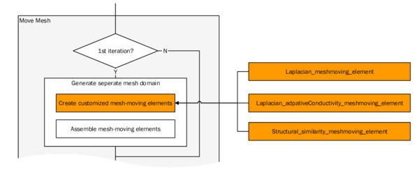
|
| Figure 161: Integration of different mesh-updating procedures into Kratos - The figure shows that the different mesh-updating procedures only require an introduction of the respective new element types into the overall ALE-simulation from figure 3 |
Let us now have a look on how this actually behaves in a simulation. To this end we firstly use two different discretizations of the above mentioned testing setup (see figure 162). In each case a translatory movement in positive y-direction will be prescribed and the covered distance until the first element collapses will be recorded.
Figure 163 summarizes the results of both cases in a diagram. Figure 164 indicates the behavior of the mesh as reaction to the imposed movement.
As can be seen from the diagram in 163 and the resulting displacement field in figure 164, the Laplacian mesh-updating procedure with constant conductivity can handle a movement of which corresponds to a significant deflection in the corresponding example where . So its advantage lies obviously in its simple formulation while already being able to handle large translatory movements. It furthermore can be stated that the method is the most robust one of the herein presented methods, since there is no parameter to adjust.
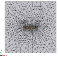
|
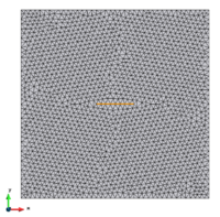
|
| (a) Non-uniform grid | (b) Uniform grid |
| Figure 162: Different discretizations of the setup from figure 160 - Both discretizations contain around 2000 degrees of freedom and 3500 elements | |
Now consider the case where there are areas of the domain that contain elements of the same or almost equal size as shown for some extreme case in figure 162b. Here the above mentioned trick of omitting the multiplication with , i.e. the volume or area, does not have any effect leading to a significant worse performance as the diagram in 163 shows. A much smarter approach thus would be to adapt the rigidity of a mesh element according to some other criteria than simply the volume. Some measure of the elemental deformation can be used instead.
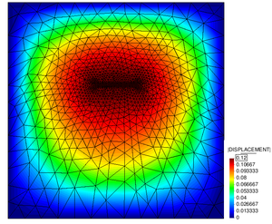
|
| Figure 164: Resulting mesh-movement in case of a Laplacian mesh-updating procedure (const. conductivity) - The pictures show the results after a prescribed . |
This idea of enhancing the Laplacian mesh-updating procedure by introduce an adaptive elemental rigidity that adapts to the local deformation, poses the second of the implemented mesh-solver. The latter is going to be described in more detail in the following.
To reach this enhancement we have to, from a theoretical point of view, introduce a function
|
|
(8.9) |
i.e. an adaptive conductivity into 8.5. As already pointed out we need a criterion or deformation measure in order to be able to locally adjust the conductivity. It is obvious to take therefore some norm of a formulation of the elemental strains. Here principally one can choose between the various existing strain formulations. Since the elements are expected to collapse earlier in compression than in tension it is obvious to take a strain measure that does not converge to a finite value in the compressive limit case, such as for example the Euler-Almansi strains. The implementation of the nonlinear Euler-Almansi strains as a mesh-updating procedure, though, is not straight-forward. Sticking to the focus of this monograph we will thus use the linearized Euler-Almansi strains and leave the enhancement to the non-linear counterpart to future projects. The linearized Euler-Almansi strain tensor is defined as2:
|
|
(8.10) |
where is the current displacement and the deformed reference configuration. Now, to define the conductivity, we take the Eucledian or Frobenius norm from . The adaptive strategy hence reads:
|
|
(8.11) |
The latter can now be used in 8.5 to form 8.8 which again can be solved in Kratos. From an implementation point of view this updating strategy was again implemented as new element formulation in Kratos as indicated in figure 161. Additionally to this adaptive conductivity, as done for the first Laplacian mesh-updating procedure, we are omitting the multiplication with . As a result we obtain a mesh-solver that takes into account not just the size of each single element but also the deformation it experiences. This is in particular advantageous with rotatory movements.
Using the above test case of a rotatory movement with non-uniform grid, the results can be quantified looking at the diagram in figure 165. It clearly can be observed that for the Laplacian mesh-moving strategy with adaptive conductivity the rod undergoes a much higher rotation until the first element collapses compared to the case where we consider all elements to conduct the prescribed movement equally.
Figure 166 illustrates the effects for the case where we prescribe an angle of . It clearly can be seen that with an adaptive conductivity the mesh gets more rigid at spots with a high deformation, i.e. at the circumference of the circular path, and spreads the movement better into the domain compared to the case where . This leads to an overall more balanced mesh.
There are, however, still problems occurring. Consider the case where we have very stretched elements. In this case, the gradients
|
|
(8.12) |
tend to zero which renders the conductivity zero and hence turns equation 8.8 to a trivial statement, which is not allowed. That is for very large deformations, as e.g. in rotations, artificially overstretched elements tend to form out as can be seen in figure 167a. As a consequence the mesh-updating will fail earlier as one might expect with this adaptive improvement.
So in a nutshell: With making the conductivity adaptive to a simple local deformation measure we can already get a significant improvement of the mesh-updating procedure with just very small changes in the original Laplacian algorithm. Also the procedure can be regarded as very robust since there is still no parameter to adjust manually. We are, though, still facing numerical artifacts that may arise with very high deformations. Deformations of this kind, however, were expected from the later intended FSI-benchmarks, so a further improvement was to be included.
One of the essential characteristics of the aforementioned Laplacian strategies is the componentwise decoupled consideration of the mesh-movement. That is, a movement of the mesh-boundary in one of the cartesian directions will not lead to an update of the position of the mesh-nodes in all the other directions. That might lead to drawbacks with movements that result in a shear dominated reaction. This indeed can be observed in the example of the rotating rod. Due to the decoupled consideration in the aforementioned Laplacian mesh-moving strategies, the mesh nodes will only be moved in tangential direction of the rotating rod as shown by the respective vector field of displacements in figure 168a. As a consequence the elements close to the rod tend to get stretched and aligned which initiates the problems that are shown in figure 167a.
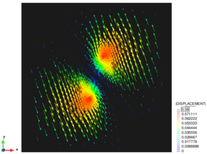
|
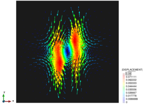
|
| (a) Laplacian with adaptative conductivity | (b) Structure-like |
| Figure 168: Displacement field with a Laplacian and structure-like mesh-updating - The picture shows the corresponding vector fields to the results shown in figure 167. Note that elements in case b) will be reoriented due the artificial material flow. | |
To reduce the stretching effect one can introduce a mesh-updating procedure that takes into account shear effects. One easy and at the same time effective way of how this can be achieved is to assign a structure-like behavior to the mesh3. I.e. we treat the separate mesh-domain in the ALE formulation as separate structural problem with own material characteristics and with the given movement of the mesh boundary as respective Dirichlet boundary conditions. This is what is done in the third and last type of mesh-updating procedure of this chapter.
In this procedure, we are again solving equation 8.8 for the unknown displacements of the mesh. But this time the classical linear elemental stiffness matrix for a linear isotropic material4 is used therefore. Nevertheless to again let smaller elements behave more rigid, we still omit the multiplication with . That is we compute the elemental stiffness as
|
|
(8.13) |
In there and is the material matrix. Note that by introducing a linear isotropic material we implicitly introduced a parameter, i.e. the Poisson's ratio 5, which the user can choose arbitrarily. By varying it the mesh-updating procedure can be tailored to the specific problem. Since the optimal parameter value is, however, not known a priori and may vary significantly, this procedure has at first to be assumed as less robust as the simple Laplacian strategies before.
The implementation of this updating procedure corresponds to the one in the Laplacian case. That is a new type of element was formulated and integrated into the given FEM environment. Applying the structure-like mesh-updating procedure hence requires a computation of the mesh-movement with the newly implemented elements.
The above mesh-solver was tested using the rod with a prescribed rotatory movement and a parametrization of , which basically imitates a steel-like behavior. The results are quantitatively compared to the ones from the adaptive Laplacian mesh-moving strategy in the diagram of figure 169. With an almost higher angle until the first element collapses the structure-like updating strategy performs significantly better making it to the most powerful up-dating strategy compared to all the other aforementioned ones. In fact this is due to the consideration of the shear movements which were neglected in all the Laplacian strategies. This can be seen when comparing the different resulting mesh-movements as done in figure 167. The Laplacian movement clearly tends to stretch the elements whereas in the structure-like case the elements itself will be re-oriented following the physical shearing behavior that the prescribed movement of the mesh boundary introduces. This will keep the elements well shaped for a longer time. The reorientation gets obvious when having a look a the vectors of the resulting displacement field which are shown shown in figure 168b.
The treatment of the mesh as a structure, however, may also sometimes lead to unexpected results, in particular when the moving structure is close to the domain border. Here the treatment of the mesh as continuum may lead to areas where the different mesh nodes of an element move in opposite direction. This can be observed when letting the above described rod again translate in positive y-direction and update the mesh using the structure-like mesh-solver. The corresponding results are shown in figure 170.
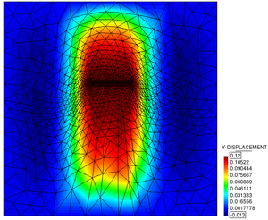
|
| Figure 170: Drawbacks in the resulting mesh-movement in case of a structural mesh-updating procedure - The pictures show the results after a prescribed . Note the difference in how the elements are oriented in the vicinity of the rod edges compared to the results obtained for the Laplacian updating shown in figure 164 |
In here we see the natural material flow that can be expected, i.e. nodes above and below the rod are pulled upwards whereas the nodes in the outer region are forced by the near boundaries to move downwards. This artificial material flow will force the elements at the edge of the rod to rotate, which leads to a comparatively early collapse of them. In fact this behavior can be quantitatively detected when comparing the possible translations in case of the structure-like updating procedure and the Laplacian mesh-solver from earlier in this chapter. The comparison is shown in figure 171. As can be seen in the diagram the Laplacian updating performs significantly better in this case since it does not cause the aforementioned artificial material flow.
At this point it can be summarized: For a translatoric behavior the Laplacian mesh-solver performs better than the structure-like strategy. In cases, however, of rotatory movements, including those where a rotation is superposed to a translatoric part, the Laplacian updating strategy suffers from the missing incorporation of shear effects. In the latter cases the structure-like mesh solver performs the best, even though the implementation of the adaptive conductivity significantly improves the performance of the Laplacian solver w.r.t. rotatory movements.
What was not taken into account in this evaluation so far and what is to be discussed in the following is the numerical effort that each updating procedure is causing. To this end again the scenario of the rotating rod is to be investigated in conjunction with the application of the three different mesh-updating procedures. In order to allow conclusions w.r.t. their practical application the example of the rod will therefore be extruded to the third dimension transforming it to a plate. See figure 172) for the respective setup.
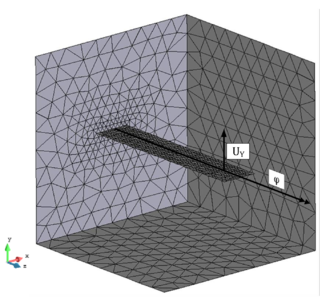
|
| Figure 172: Infinitely thin and moving plate within a fluid flow - The picture shows a setup to test the computational costs related to the different mesh solvers. |
To measure the computational effort we will rotate the plate incrementally up to and for each increment and each procedure we measure the time needed to update the mesh. The maximum time needed will finally characterize the numerical effort of each updating procedure. Table 10 lists each of the representative results.
As can be observed form table 10 the time with each of the implemented improvements almost doubles, whereas the structure-like procedure is the most demanding - as expected. Interesting to see is that just the simple introduction of one more computation step in the Laplacian case, i.e. the computation of a strain measure, already leads to a doubling of the numerical effort.
In view of the significant effort that has to be spent in any case regarding the updating procedure, it is obvious to think about techniques to speed up this process. Here the in chapter 4.1.4 described MPI-parallelization comes into play. All the aforementioned mesh-updating procedures have in common that they physically generate a separate mesh-domain, provide it with customized elements and compute the resulting mesh-movement according to the implemented elemental characteristics. In that regards it seems natural to divide the domain in different partitions, spread them among several processors which each compute the results locally for the respective nodes6. Depending on the size of the domain one can by that expect a significant speedup of the computation time.
| Laplacian | Laplacian adative | Structure-like | |
| dofs [-] | 78,000 | 78,000 | 78,000 |
| tetrahedra [-] | 460,000 | 460,000 | 460,000 |
| Computation time [s] | 5.24 | 10.04 | 17.65 |
This approach, however, implies of course setting up a communication plan at the interface between the different partitions7, which will bring some overhead along. In order to test the possible speedup in this context, the 3D setup described in figure 172, where the plate is turned around its lateral center axis, is utilized. In here we apply an angle of , then update the mesh with the structure-like mesh-solver and measure the time needed for the respective computation. This is done using a varying number of processors. Figure 173 shows the results for two different domain discretizations.
Besides of the speedups that one can observe, which are with up to almost accelerating the simulation time significantly, three facts are striking. First as one can expect, the higher the number of degrees of freedom the less the relative overhead which leads to generally higher speedup values for very large models.
In all the tested models, however, one can at some point observe a decreasing tendency which means the program runs slower again with an increasing number of processors. In parallel computing this phenomena is called parallel slowdown and is usually an indicator for a bottleneck in the communication. It is obvious that this bottleneck arises here due to the fact that when exceeding a certain limit number of processors, each processor is only processing a fraction of the originally very high number of degrees of freedom. This leads to a relatively high communication effort compared to the actual simulation time each processor needs. In fact, and this is the second interesting result, with all the tested mesh-updating strategies, the speedup starts to drop around
|
|
(8.14) |
as can be seen from figure 173c. This relation of course is not of a general nature, but can serve in the scope of the application of the above discussed mesh-solver as a first idea of how many processors should be used in a parallel run for a given number of degrees of freedom.
Third striking result is the fact that for the case of a very high number of degrees of freedom, the simulation indeed scales significantly until some processors, the efficiency, however, very quickly drops from to values of and well below. As a consequence the desirable linear scaling is only observed up to some processors. Above we observe a worse gradient. The effect is accordingly higher for the case where we have lesser degrees of freedom. This clearly indicates that, even though the implemented parallelization is already able to speed up the simulation significantly there are still improvements possible. One can for instance think of a better organization of the communication pattern among the single partitions, but this lies far beyond the scope of the present work.
Having tested now both the numerical effort and the capabilities of the three different mesh-updating procedures, we can summarize the results and set them into a general context which can help to identify the proper method to use in future applications (Figure 174).
Note that in general the effort connected to the mesh-updating is quickly growing8 as the number of degrees of freedom increases making especially the structural solver very expensive compared to the actual simulation time. For instance, from table 10 we can see that for the case of degrees of freedom in a serial approach the single mesh-update already lasts in the range of almost .
Based on experiences that were made within the scope of this work, the application of the structure-like mesh-solver for models with more than 1,000,000 degrees of freedom multiply the actual simulation time significantly which is why we distinguish between cases above and below this value in figure 174.
Despite now having options to deal with various types of movements in an FSI-scenario, the strategy of updating the mesh might not be powerful enough for a robust simulation, especially if the displacements are very large and complex. In fact in a body-fitted approach there will always be a limit beyond which a proper mesh-update is not possible. So in cases where we are facing critical movements, changing the mesh-solver is not always an option. As a matter of fact, the larger and more complex the movements are, the more attractive alternatives get. Two of those alternatives, the embedded method and some remeshing strategy, are indicated in the overview from figure 174. In the present monograph, we are interested in the embedded method. Which kind of movements the embedded method can handle in contrast to the above elaborated possibilities with respect to the body-fitted approach is going to be topic of the next chapter.
(1) Remember that is directly related to the elemental volume or area
(2) Note that with a linear description of kinematics the different strain measures merge into this single linear formulation.
(3) Effective since the framework of a structural FEM-analysis is already present and can be fully utilized for this purpose.
(4) Plane strain in case of 2D.
(5) The Young's Modulus does not affect the mesh-movement
(6) From an implementation point of view this was done by parallelizing the blocks “Generate separate mesh domain” and “Regenerate separate mesh domain” in the original process-flow depicted in figure 3.
(7) The respective theory is explained in chapter 4.1.4
(8) Also in a parallelized run.
8.2.2 Possibilities and limits w.r.t. movements in an embedded approach
Neglecting a costly remeshing, the body-fitted approach has clear limits set by the capabilities of the specific mesh-updating strategy. Large movements might thus get very hard to handle and rotatory or superposed movements are commonly impossible unless they are not occurring on fair scales. A practical application by contrast may require an incorporation of large and complex movements in an FSI-analysis. This is where the embedded method comes into play. The fact that in the latter approach the two different domains are handled separately and the wet interface is continuously tracked using the given distance function has obvious advantages in this context and opens the door to a wide range of possible applications. It, however, requires to think about new questions that arise in conjunction with the embedded geometry. Two of the most important questions are:
- How to deal with the fact, that nodes may be outside the fluid domain (i.e. inside the structure) in one instance and jump into the fluid domain in another?
- How to deal with the fact that the quality of the tracked interface, and by that the geometry of the represented structure, may vary when the movement extends to different refined sub-domains of the fluid?
These questions shall be discussed in the following. Eventually we will be able to comment on the movements that are possible within an embedded approach.
One of the most striking advantages of the embedded method is the fact, that it can principally handle arbitrary movements which in other cases would either lead to significant errors due to badly shaped elements or require a complete remeshing. Both is typically to be avoided. Figure 175 gives an example in terms of possible movements in an embedded approach. In there a clock-wise rotatory movement of a membrane is analyzed. The setup corresponds to the high-Reynolds flow setup from figure 154. The prescribed circular frequency is chosen to be small compared to the inlet velocity such that no mixing occurs:
|
|
(8.15) |
It is seen from the figure, that the rotation can be arbitrarily resolved which allows to capture the different flow characteristics for the different angles of attack in one simulation run. In fact, since we are embedding the structure it is not even required that the rotation of the membrane, or the movement of the embedded structure in general, has to take place inside the fluid domain. It can also partially or fully leave it1. It is obvious that these movements combined in one simulation can not be handled in a body-fitted approach without significantly increased computational effort.
The setup in the given figure is, however, still omitting a big problem all embedded approaches have in common. I.e. the fact that nodes may change their domain membership as a voluminous, rather than an infinitely thin, structure is moving through the fluid. In this case we conceptually have two different regions in the fluid domain: an active region, which is not directly affected by the embedded structure, and an inactive region, where the fluid nodes fall into the embedded structure domain, i.e. are actually outside the fluid or inside the structure. It is obvious that fluid nodes may change their domain membership as the structure is moving.
In the case where fluid nodes are leaving the fluid domain and heading into the domain of the structure, the change in the domain membership can by handled in a straightforward manner. Since they become inactive we can set the corresponding state values to zero to effectively exclude the corresponding degrees of freedom from the CFD solution. The other case where inactive fluid nodes become active again requires a more evolved approach since they have to adjust to the surrounding flow characteristics. To this end one has to distinguish the two cases depicted in figure 176.
Case 176a is a standard case of the embedded approach. Here one has to find mapping routines that map the velocity of the embedded structure nodes to the nodes of the cut elements of the surrounding fluid domain. Respective techniques are discussed in chapter 8.3. Case 176b is somewhat different. Here the structure has a velocity so high that in one instance the embedded domain is releasing several subsequent fluid elements. The corresponding adjustment of the state variables clearly cannot be covered by mapping techniques without applying some kind of neighbor-search which typically is very expensive. So the question is how to set the state variables of nodes that are moving from outside the fluid domain into the latter and that are not covered by some mapping techniques?
In fact solutions for this problem are of essential importance in an embedded approach since they may affect the accuracy in the vicinity of the interface significantly. In particular when high velocities are present. Advanced techniques might incorporate to this end some projection of the given velocities from the closest structure node. Due to the continuum assumptions and continuity conditions this might be already a very good approximation that will reduce a possible accuracy loss significantly. The development of techniques of this kind is, however, left to follow-up research activities.
In order to be able to run first FSI analyses anyways, a very simple approach was used instead. In that we let the respective nodes freely evolve from zero, as soon as they hit the border into the fluid domain. How this is affecting the solution of an FSI problem is to be investigated using again the example of a cylinder in a channel flow as given in figure 157. To simulate an FSI scenario we are at this time using a coupling of the velocities and prescribe the cylinder movement by
|
|
(8.16) |
which basically is a periodic movement in around the center of the channel and starting from a left-most position of . The latter movement implies a velocity of
|
|
(8.17) |
and hence a maximum velocity of . Note that the Reynolds number in this setup is changing according to the relative velocity given by
|
|
(8.18) |
Here we choose 2. This yields for the movement in positive x-direction an and for the one in negative x-direction an .
Looking at the Reynolds number at first, we expect from a physical point of view for the movement in positive X a steady laminar flow field whereas for the opposite movement the formation of some laminar vortices, which according to [55] start at around . Figure 177 poses the corresponding results. Note that the embedded cylinder appears as domain with zero velocity and pressure. The very rough geometry depicted is just due to still given visualization limitations. The cylinder as it is actually seen from the fluid solver is shown in figure 178.
As can be seen from the results, the principal physics is captured in the analysis and we do not get any instabilities arising from the above introduced simplifications of letting the state variables evolve from zero. In terms of the FSI-simulations later, this indicates an adequate handling of the active and inactive fluid nodes. Remarkable in the results from figure 177 is, however, the simulated pressure field. Looking at the two different time instances, first with a low and then with a high relative velocity, we observe that the pressure tends to form striations. This problem originates in the fact that the state variables of fluid nodes directly next to an immersed boundary are treated differently from the state variables of nodes further inside the fluid domain, as figure 176 illustrates. In the first case we apply mapping techniques whereas in the latter case we let the state variables evolve from zero. Having an incompressible flow, this different treatment directly affects the nodal pressures which as a result may show significant local variations. These variations may eventually lead to striations as the structure moves through the fluid. The latter becomes the more significant the higher the relative velocity is. In conclusion this means that even though the simple approach of letting the state variables evolve from zero can be sufficient for a stable solution, accuracy losses have to be expected later on. Having in mind, however, that future research is necessary to minimize this additional accuracy loss, we can run first FSI simulations based on the embedded approach.
Besides of nodes that are changing their domain membership as the structure moves through the fluid we have to deal with another important problem:
In order to represent the boundary of the structure properly, the discretization of the fluid domain, in the following also referred to as the background mesh, has to be sufficiently fine in order not to introduce significant approximation errors. Typically, however, one is not able to refine the background mesh equally fine due to computational limitations. So one might concentrate the refinement to the area to which the expected structure movement extends. Even this, however, may lead to an explosion of the computational costs for large movements and big domains. So with an embedded formulation of an FSI-problem one has to deal with the fact that the representation of the structure only can be as good as the background mesh allows (which may vary along the movement). In the best case this only affects the accuracy of the fluid solution slightly. In a worst case scenario by contrast, this accuracy loss may even affect the entire dynamics of the flow and hence yield significantly different results for the coupled system.
How much the results can change is shown in figure 179 at the example of the resting cylinder in a laminar flow field. As already seen in earlier results (figure 158) the setup should actually yield a steady-state flow solution. Given a very coarse background mesh as in 179, however, the solution with the embedded approach suddenly changes to a different, i.e. transient one. The reason can be found when looking at the embedded cylinder and how it is seen from the fluid solver according to the implemented distance function. The in this case insufficient discretization leads to a boundary representation of the cylinder that contains small edges. The latter are just big enough to critically influence the flow such that we obtain an overall dynamic behavior. So essentially we observe a strong dependency of the solution on the quality of the background mesh. While this may sound obvious, it is of utmost importance to realize that the quality of the background mesh can change significantly along the way the structure moves.
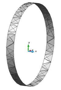
|
| Figure 178: Embedded cylinder - The picture shows how the embedded cylinder is seen in the simulation from figure 177 |
In order to deal with this problem, local refinement strategies can be introduced. Unlike in a body-fitted formulation, however, it is not enough to refine the given interface once in the embedded approach. Rather, since the intersection pattern may change significantly if the structural response extends to a large fluid domain along the simulation, a continuous refinement is required. A simple possible algorithm, which to this end was developed and used in the scope of the present monograph, is given in figure 180. The actual refinement strategy is adopted from [53]. The algorithm basically marks all fluid elements that are cut by the structure as well as their direct neighbors. This is done by means of information from the distance function. The algorithm then refines the marked elements and tags the resulting smaller elements as ``IS_REFINED". The latter makes sure that elements are not refined twice which would immediately lead to an explosion of the number of elements. How this refinement step is integrated into the overall process is indicated in figure 181.
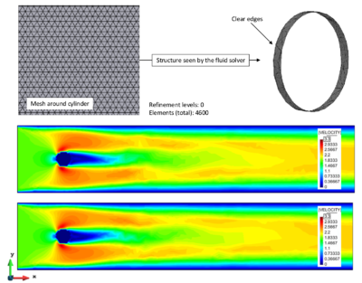
|
| Figure 179: Transient flow due to bad approximation of an embedded structure - The figure shows the resulting flow field for two subsequent time instances. |
Applied to the above mentioned problem of the badly represented cylinder it is possible to resolve the boundary accurate enough to get the expected steady-state flow solution. The corresponding results are shown in figure 182. It is important to note, though, that the higher the Reynolds number the more sensitive the flow reacts to small edges on the structure which in turn requires the mesh to be all the more refined in order to not cause artificial flow separation or similar effects. For instance if in the given example the Reynolds number is increased from by factor of to , we will again observe a transient flow solution which actually would require a further level of refinement. It is obvious that this very quickly cannot be handled anymore due to computational limitations. So generally one can conclude that, at the moment of writing, the given embedded approach is clearly not suited for problems with very high Reynolds number, not just due to accuracy limitations but also due to the connected computational costs with regards to the necessary refinement.
| Figure 180: Pseudo-Code of the applied refinement strategy |
But not just when the Reynolds number is very high, but also when the structural response is very large, the number of degrees of freedom explodes with the aforementioned refinement strategy. Figure 183 illustrates the situation at the example of the cylinder when it starts to move through the domain3. The diagram from 184 quantifies the observation.
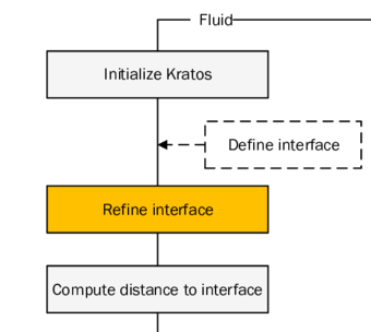
|
| Figure 181: Implementation of the refinement strategy - The picture shows how the above mentioned refinement strategy (orange) is integrated into the overall Kratos specific work flow of the embedded method shown in the introduction(4). |
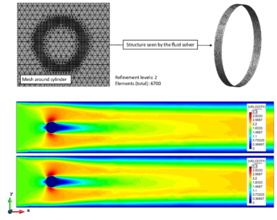
|
| Figure 182: Influence of the given refinement strategy - The figure shows the resulting flow field for two subsequent time instances. It can be seen that the given refinement strategy may resolve problems occurring due to approximation errors w.r.t the embedded structure. Note in this context the steady-sate solution in contrast to the transient one given in figure 179. |
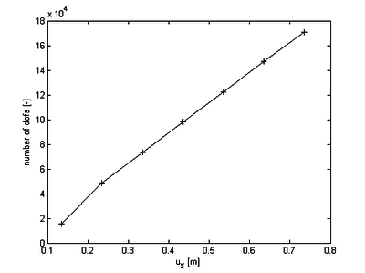
|
| Figure 184: Increase in number of dofs due to local refinement - The picture shows the resulting number of dofs for the situation in figure 183 after local refinement along the translation in positive X-direction |
Here the computational costs obviously increase enormously both due to the time needed for the refinement as well as due to the resulting time for the computation. So the refinement is clearly counterproductive in cases of large movements or deflections within an FSI scenario. Since, however, the embedded method is particularly powerful in these applications, it generally holds that, introducing refinement strategies into an embedded approach calls to the same degree for an introduction of coarsening techniques, otherwise the computational effort grows beyond any reasonable limit. Further developments and investigations in this context will, however, be part of future research.
Linking now all the above discussion again to the questions stated in the very beginning it can be concluded: In cases where the interface needs to be particularly well represented, since otherwise crucial errors such as unexpected flow-separation etc. may arise, a very fine background mesh is necessary which in turn requires powerful and smart refinement strategies. To this end a simple but robust refinement strategy was suggested. Every refinement in an embedded approach, however, again requires coarsening in order to keep the computational costs bounded. Coarsening techniques becomes particularly important when the simulation is facing very large movements. Developments in this regard will be part of future research.
In terms of fluid nodes that change their domain membership, two situations could be identified: Cases where inactive fluid nodes jumped far into the active fluid domain and cases where they are still part of the cut fluid element. It could be shown that handling nodes in the former situation is difficult since we do not have direct access to state information of the structure that just released the nodes. A simple first approach was chosen here which lets the state variables evolve from zero. This, however, introduced clear accuracy errors depending on the movement. More elaborate strategies will be part of future developments. In terms of the second situation it already was mentioned that here mapping routines will ensure a proper exchange of the state information at the interface. Which techniques are used for this purpose and how accurate they are is going to be discussed in the next chapter. After having then the movement and the data exchange complete we will subsequently be able to carry out FSI analyses based on the embedded approach.
(1) This at a first glance might look unnecessary but one can for example think of a watergate that arises from the ground of a channel flow.
(2) Note that intentionally this is a different value as given in figure 157
(3) The reason for the movement might be of any kind and is not of importance here
8.3 Mapping of quantities between the physical domains
The last step to a full FSI-simulation is to establish the coupling of the quantities of interest between the physical domains and the corresponding proper data exchange. In the body-fitted case this is straight forward for an interface with matching grids. For the case of non-matching grids specific mapping techniques are applied to transfer data between different discretizations as already seen in earlier chapters. In case of an embedded solution approach the data exchange is, however, somewhat different. Indeed we also need to exchange field information among two different discretizations but here we have no common interface as in the body-fitted approach which requires more advanced mapping techniques each dedicated to the single solution quantities that need to be exchanged. For an FSI simulation this means that we need to couple the fluid pressure to the structure by means of pressure mapping techniques and have to make sure that the inverse coupling of the velocities is established, too, by means of velocity mapping techniques. How this is done in the embedded solution procedure is going to be topic of the present chapter.
Both mapping steps can be principally performed in various ways. With the choice or the development of a proper technique, however, we have to take into account the intrinsic difference w.r.t to the pressure or the velocity transfer, respectively: The pressure mapping essentially corresponds to an interpolation of given scalar values to a target node, while in contrast to that the mapping of the velocities is an extrapolation of a vector to several different nodes, namely the intersection nodes, that again expect vectors. Figure 185 illustrates the situation.
This means that while we are basically able to use well-known and efficient interpolation routines for the pressures, incorporating extrapolation techniques for the velocities is significantly more difficult. Furthermore, since the extrapolation in the latter case requires generally operations with tensors of seconds order, it has also to be considered as very costly. All the mapping techniques that will be described within this chapter, are chosen according to these preceding considerations.
In this context we will start in the first section with the discussion of the developments related to the pressure mapping, in whose course we will present three different approaches. These approaches will be tested and compared to each other both qualitatively and quantitatively by means of a common benchmark example. Thereby it will be seen that, despite the developed techniques are yet ready for an application in an FSI-simulation, a crucial challenge persists. The latter is going to be discussed in the follow-up section. At the end of this chapter we will finally present a solution for the velocity mapping which is of a more pragmatic nature and avoids complex tensor operations. Having eventually both steps working, we can go for fully coupled FSI-simulations. The latter are going to be topic of the remaining chapters in this monograph.
8.3.1 Pressure mapping
In pure incompressible flow problems the pressure appears as a Lagrange multiplier that adjusts to the velocity field such that the incompressibility constraint is fulfilled. In that sense the pressure plays a minor role compared to the velocity and is typically only computed as accurate as necessary to comply with the incompressibility condition. The situation is, however, different in an FSI-scenario. Here the pressures are the driving quantities that put the structure into motion, which is why they have to be computed much more accurate in comparison to the pure CFD analysis. This has to be considered with the choice of a proper pressure mapping technique.
Principally there are various possible techniques to map the pressure from the fluid domain to the structure, ranging from simple arithmetic operations up to elaborate projection procedures. The choice which one fits best to the given application is hence a classical choice that is driven by the aim of balancing out implementation or computational effort, robustness and in particular, as indicated, accuracy. In this context three different techniques were chosen to be implemented and evaluated:
- Arithmetic averaging
- Radial basis interpolation
- Interpolation based on the discontinuous shape functions1
All the aforementioned methods shall in the following be discussed critically. At the end of this chapter the reader will be able to estimate the capability and drawbacks of each method and hence can make his own choice among the given possibilities in case of an application.
For the sake of a proper comparability a common test case is used. In here a hollow sphere is placed in a 3D linear pressure field which in turn extends over a cubic unit volume. The setup is depicted in figure 186.
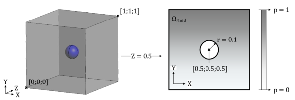
|
| Figure 186: 3D test case for the different pressure mapping techniques |
The linear pressure distribution in the fluid domain is imposed and not due to a given velocity field. Thus it simply reads:
|
|
(8.19) |
where is the vertical position coordinate. Since the sphere is embedded in the fluid domain, this pressure distribution has to physically appear as face pressure on the surface of the sphere. Given the dimensions of the sphere from the figure this implies and . Assuming now a “perfect” mapping routine, the face pressure of the sphere has to reproduce the linear distribution between and exactly. All deviations are only due to the inherent inaccuracy of the applied technique. This fact is used to discuss the accuracy of the given mapping methods in the following. Unless not explicitly highlighted else, the discussion is valid for both the positive and the negative face of the sphere alike, which is why mainly results for the positive face will be shown. We will start with the simplest given method, i.e. the arithmetic averaging.
The arithmetic averaging requires, as well as all the following mapping techniques, as a first step a bin-search to identify the position of the single structure nodes within the fluid domain. That is, each structure node is assigned to the fluid element in which it lies. This is important to identify which pressure values of the fluid actually have to be mapped to the structure. To this end we use the procedures that were introduced in chapter 4.2. Once the position of each structure node within the fluid is known one has to distinguish two situations:
- structure node lies within a fluid element that is actually cut by the structure,
- or the structure node occurs within a non-cut element which typically happens at the structure boundary or with curved structures in general.
In the former case the idea of the arithmetic averaging is to average all pressure values of the cut fluid element each for the positive and the negative face of the embedded structure 2 and assign the two resulting average values to all included structure nodes as positive or negative face pressure, respectively. Figure 187 explains the principle. For a better understating the situation is explained in two dimensions. The principle is, however, the same in 3D. This approach is applicable for all kind of intersection patterns where the distance function identifies a clear pressure terminator within the affected fluid element.
While in the latter situations the mapping is straightforward, it becomes more difficult in cases where the fluid element is not considered as cut by the distance function, but nevertheless contains structure nodes. A representative situation is depicted in figure 188 where the structure cuts a single edge and looms into the fluid element. This is typically the case in the vicinity of the structure boundary3.
In these cases we are lacking information in terms of the orientation and position of the embedded part of the structure. As a consequence the pressure field within the affected fluid elements will not be discontinuous which is why we cannot distinguish between positive and negative face pressure here. Nevertheless physics requires an assignation of positive and negative face pressure to the structure. So the question is now how to assign the different face pressures without being able to distinguish the latter? As obvious this leads in any case to approximation errors. Important to note is, however, that the resulting approximation error is not due to a drawback of the mapping technique but, as detailed later, rather more a consequence of the intrinsic approximation error in an embedded approach. This error might lead from a slight accuracy loss up to severe stability problems in the simulation and so requires elaborate remedies.
With the pressure mapping using the arithmetic averaging, we face this problem by assigning both to the positive and the negative face of the structure the averaged pressure from all the nodes of the relevant fluid element (figure 188). As a consequence the structure's nodal response in this point will not be affected by the pressure at all, which in any case would lead to a wrong behavior. By doing so, it is rather more only driven by the movement of the adjacent structure nodes that are not having this problem. This balances out the structure at this point and so by construction reduces the problem to a minimum which eventually yields a more robust algorithm.
Applying now the algorithm to the above defined benchmark for two different levels of refinement of the fluid domain, representing a coarse and a fine mesh, one can observe the results summarized in figure 189.
First striking result that can be observed is a strong dependency of the mapping quality on the refinement of the background mesh, i.e. the fluid mesh. That in turn means that a proper tracking of the interface is not just important in terms of geometrical considerations or separation phenomena but is also essential for a proper representation of the pressure field. In fact, since the pressure is the driving force for the structural behavior, a proper FSI simulation is only possible if the interface is adequately captured which raises the importance of powerful refinement techniques even more.
Second striking fact, when looking at the pressure iso-lines and the extreme values, is that already with a simple averaging at an adequate refinement level, the linear pressure field can be captured very well with deviations of the extreme-values only in the order of . So the averaging can be considered to be already very accurate. Later on, this will be quantitatively enforced in a comparison with the remaining methods and the analytic solution. Moreover, due to a parameter free formulation, the method can also be regarded as very robust and stable. The combination of both adequate accuracy and superior robustness with its negligible computational cost makes this method very attractive for an application in an FSI scenario.
There is, however, an important drawback of the arithmetic averaging. What was not mentioned so far is, that the latter actually is not an interpolation routine in which a transient pitch from the given pressure values of a cut fluid to the embedded structure is taken into account. This becomes all the more important the more the intersecting structure approaches the edge nodes of the tetraheda. In this cases we are overestimating the influence of the pressure values from the nodes that are further away, as figure 190 illustrates. This error can be considered as small but nevertheless can be avoided by using interpolation techniques rather than the simple averaging. A very famous technique to this end is the radial basis interpolation or radial basis method (RBF method), which is going to be discussed in the following.
In terms of the RBF theory we closely follow chapter 1 in [56] while sticking here to the “basic RBF method” and its main ideas. In the latter dissertation the RBF method is elaborated from an application oriented view whereas e.g. in chapter 1 & 2 of [57] a more mathematical rigorous description can be found.
The objective generally in the RBF method is to interpolate between given scattered data, which in our case are given as the nodal pressure values at the intersection points within one cut fluid element. The idea of the basic RBF method is now: for a given set of data points and corresponding data values , a set of basis functions is chosen such that a linear combination of these functions satisfies the interpolation conditions
|
|
(8.20) |
Based on this, the actual interpolation reads
|
|
(8.21) |
where is the Euclidean norm and is a radial distance making to some radial function that gives the method its name. The coefficients are determined from the interpolation conditions given in 8.20. The corresponding symmetric linear system of equations reads
|
|
(8.22) |
where is the interpolation matrix whose entries are computed with the given scattered data values as . This system can be solved with standard procedures. Knowing after the solution the coefficients we can finally use 8.21 to compute for an interpolation value at any .
Transferred to the given problem of the pressure mapping this leads to the procedure illustrated in figure 191. The pressure mapping using the RBF method is basically a solution of equation 8.21 for the structure node at within a cut fluid element - each for the positive side ()and the negative side () of the structure, respectively.
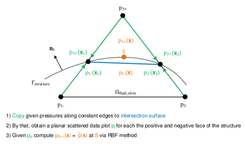
|
| Figure 191: RBF interpolation as pressure mapping technique - The picture illustrates the principal procedure how the pressure of a cut fluid element is mapped to embedded structure nodes. |
Now let us have a closer look on the basis function . As already indicated it is necessary for the solution to chose a type of basis function . In order to prevent from becoming singular, has to satisfy certain conditions regarding which the reader is referred to respective literature. Instead, a list of possible shape functions, adapted from [56], shall be given in table 11.
From an accuracy point of view one generally prefers the infinitely smooth RBFs here. They, however, have in common that they are all relying on a parameter , which has to be estimated. One typical method to determine, rather than to manually guess, a parameter estimation to this end is e.g. the maximum likelihood estimator or MLE. The latter and other alternatives are described in part F of [58]. Implementing routines like the MLE was, however, far beyond the scope of this monograph, so the was chosen manually for the purpose of the pressure mapping.
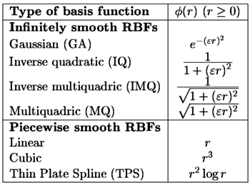
|
Applying now the RBF method to the benchmark of the sphere from the beginning, one can observe the results depicted in figure 192a. For the latter computation an infinitely smooth basis function, i.e. the Gaussian function from table 11, was used together with the estimation of , which corresponds to the maximum length between two intersection nodes within a cut fluid element.
As one can observe, the results are strongly deviating in both the distribution, where the linear gradient is clearly not represented, and the extreme values, where local spots that significantly exceed the analytic extrema are visible. Obviously this is due to a bad estimation of which leads to an ill-conditioned interpolation matrix . This can be seen when instead of the parametrized infinitely smooth basis function a parameter-free piecewise function, i.e. the linear function, from table 11 is used. The corresponding results are shown in figure 192b. As expected the results are in this case slightly improving but nevertheless not acceptable. Actually the main problem is not originated in a badly estimated parameter, but rather more a consequence of the fact, that all the given points are by construction lying in one plane (indicated as blue line in figure 191). Effectively this means that we are interpolating in three dimension whereas we only have information given for two dimension. This leads to significant deviations when computing an interpolation value for a structure node which is not lying on the above mentioned plane.
To remedy the aforementioned drawbacks the pressure mapping strategy using radial basis functions would have to be extended by a more advanced choice of the scattered data as well as a powerful parameter estimation technique. This is, however, left to future research. Instead a more robust third and last approach, that avoids these kind of problems, was developed. The latter shall be introduced in the following.
In this last approach we make use of the discontinuous shape functions. The idea thereby is to evaluate the discontinuous shape functions of all fluid elements with embedded parts at the position of the respective structure nodes and use the resulting values as weighting factors to interpolate each on the positive and the negative face between the given nodal pressures of the respective fluid element. The procedure is somewhat more complex compared to the ones described above which is why the overall process flow shall be given in advance (figure 193). Based on that the details will be discussed in the following.
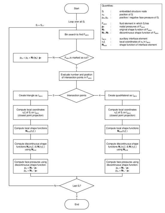
|
| Figure 193: Pressure mapping using discontinuous shape functions - The figure depicts the overall process flow to map nodal pressure values from a fluid element with embedded structure. |
As can be seen from the flow chart, the mapping algorithm loops over all structure nodes and each searches, via the given bin-search strategy, for the one fluid element in which the current structure node is embedded. With then also the pressures, that are surrounding , i.e. the nodal pressures , are known as well as the standard shape function of , i.e. .
As it is already the case in the previous strategies, before the actual mapping we first have to check whether is actually seen as cut or not. Remember that if the fluid element is not seen as cut but anyways contains an embedded structure part, we cannot distinguish between positive and negative face which is why we are assigning an equal value as positive and negative face pressure to the structure nodes here 4. Since in this case the fluid element is not assumed to be discontinuous we therefore do not need to evaluate the discontinuous shape functions but just the standard ones for which we can use given standard routines. This makes an interpolation very simple. The pressure mapping hence reduces to:
|
|
(8.23) |
where we made use of the nomenclature introduced in figure 193. For an illustration see figure 194.
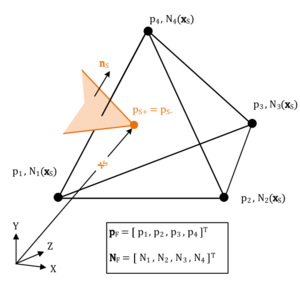
|
| Figure 194: Pressure mapping in non-cut fluid elements with embedded structure parts |
In case where is cut, the standard shape functions are no longer valid. Rather more the discontinuous shape functions and have to be evaluated. Since there are not yet standard routines for a respective operation, we will have to construct the discontinuous shape functions at this point separately. Once they are then constructed the interpolation and hence the mapping is in principle the same as before:
|
|
(8.24) |
The crucial part now is the construction of the discontinuous shape functions. The complete construction and subsequent evaluation of the latter can be reproduced in the given overall flow chart and is as follows:
Once we know that the fluid element is cut, we can assume either a situation with three or more intersection points. In this context one has to remember that with less than two intersection nodes the fluid element would not have been seen as cut and with more than four intersection nodes the distance function anyways fits a quadrilateral into the cut element. In the following we will stick with the explanation to the case with three intersection nodes for which the process of constructing the discontinuous shape functions is illustrated in figure 195. This can, however, be easily transferred to the case with four intersections.
Knowing about the three intersection points we first have to define an auxiliary triangle element that corresponds to the approximated structure and is hence representing the FSI interface in the cut fluid element. spans a local space with coordinates . For this space the local standard element shape functions can be evaluated at any position on the interface. Since the auxiliary element is dividing the original fluid element into two parts and values along cut edges are defined to be constant, we can evaluate the discontinuous positive and negative shape functions of the cut fluid element for each point on the interface by summing up the contributions of the local shape functions according to the given father-son relation between the nodes of the fluid element and the intersection points. Note that by this the partition of unity condition will not be violated. The principle is sketched in figure 195.
This now means that if a structure node lies on the auxiliary interface element, all we have to do for the construction of the discontinuous shape functions is to compute the local shape function contributions and sum them up as indicated in the example. A structure node, however, only lies on the interface for simple intersection patterns. Typically it is embedded somewhere beyond (Indicated in figure 195). The evaluation of the local shape functions, however, requires a node on the interface. To this end we need to include a projection technique where we assign to the position of the embedded structure node at in global coordinates a corresponding position in the local space. An obvious technique that can be used for this purpose is a closest point projection as shown in figure 196.
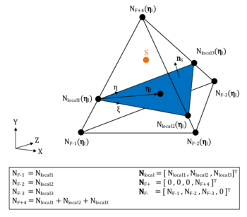
|
| Figure 195: Construction of discontinuous shape functions for pressure mapping - Note that the embedded structure node is not necessarily lying on the auxiliary interface element (blue) |
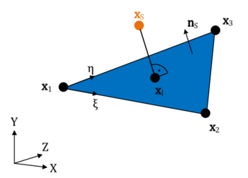
|
| Figure 196: Closest point projection to interface element |
Here we are conceptually assigning to the embedded structure node the one position on the interface, that leads to a minimal distance in between both. Speaking in global coordinates this means, that we try to find the minimum distance between and , where the latter describes the position on the interface. This can be interpreted as optimization problem that has to be solved. For the actual computation, however, we have to modify this optimization problem slightly since we want to find local coordinates for the structure node. That means our design variables are and . To this end we express in local coordinates as:
|
|
(8.25) |
where we made use of the basis vectors of the auxiliary interface element as illustrated in figure 196. Using the latter formulation, the optimization problem for this closest point projection reads:
|
|
(8.26) |
This poses a quadratic problem with linear constraints for which standard solution procedures. Being now able to project the position of the embedded structure node to a corresponding position on the local interface, the local shape functions at this point can be evaluated and summed up to form the overall discontinuous shape functions and . With them we can map the nodal pressures of the fluid element to the positive and negative side of the embedded structure node via equation 8.24
By this last function now it is possible to apply the overall pressure mapping technique based on the discontinuous shape functions to the benchmark example of the sphere from the very beginning. The corresponding results are shown for again two different refinement levels in figure 197.
The results are significantly better than the ones obtained in the RBF approach, since here we do not incorporate any parameter estimation or have to chose any specific scattered interpolation points5. By contrast the results are very similar to the ones obtained from the arithmetic averaging, i.e. a high dependency on the refinement can be observed whereas for a sufficient fine fluid mesh, the linear pressure distribution including the corresponding extreme values can be very well captured.
In fact, while this mapping method is distinctively better than the RBF approach, the difference to the arithmetic averaging is often negligible. This becomes obvious when quantitatively comparing the respective approximation errors produced by each method. Since the analytic solution of the linear pressure distribution is known and we do not change the discretization of the sphere in the different approaches, we can use a typical root mean square relative error measure for this comparison:
|
|
(8.27) |
where is the total number of nodes on the embedded sphere, the positive face pressure that was mapped to the node of the sphere and is the corresponding analytic target value of the positive face pressure at the node of the sphere. can be computed from the linear pressure distribution formulated in equation 8.28. It hence reads:
|
|
(8.28) |
Plotting the error for different levels of refinement, the graph in figure 198 is obtained. Here the single differences can be quantified. Evaluating this graph one might correctly question the point of using the more complex shape function approach for the pressure mapping instead of the easier and here even slightly more accurate arithmetic averaging. But one must not forget, that the averaging is not a true interpolation. This means that, in cases where we have a lot of intersection patterns of the kind like described in figure 190, it is expected that more distinct differences will occur in which the shape function approach will show the considerably better accuracy.
There is, however, a true drawback of the shape function approach compared to the arithmetic averaging in terms of robustness. Indeed both techniques do not incorporate any parameter so can be considered as very robust. But in the shape function approach we have to reproduce the interface in each element, i.e. we have to create which is either a triangle or a quadrilateral. If this interface element due to the intersection pattern is very small, the closest point projection described in figure 8.26 may fail since the squared values may exceed machine accuracy.
At the end of this chapter now it shall be summarized: From all the aforementioned methods, i.e. the arithmetic averaging, the RBF interpolation and the shape function approach, only the first and the latter are really suited for an application in the context of pressure mapping within the framework of an embedded approach. The RBF method is problematic since it requires a parameter estimation and a proper choice of scattering data, which leads to significant approximation errors. The other two methods by contrast are parameter-free and thus very robust. Here the arithmetic averaging is generally more robust than the shape function approach, which may sometimes fail with very irregular or highly refined meshes. In terms of approximation errors by contrast, the shape function approach is generally more accurate than the arithmetic averaging. Nevertheless in many cases, the approximation quality is comparable and may be even slightly better with the arithmetic averaging for some configurations as could be seen above. This makes the latter to a powerful alternative. Eventually only the arithmetic averaging and the shape function approach were integrated into Kratos. In view of a practical application of the mapping methods, a recommendation also based on practical experiences shall be given with figure 199.
(1) In the following also shortened as “shape function approach”
(2) Implicitly defined by the sign of the given elemental distances of the fluid elements
(3) Note that, as explained earlier, the fluid element is intentionally not seen as cut in this case.
(4) As for the arithmetic averaging. This is done to minimize possible mapping errors.
(5) Here we are truly using the nodal pressures that are spatially given in each fluid element.
8.3.2 Persisting problems with pressure mapping
Having now demonstrated the capability of different pressure mapping strategies as well as each their limitations, a still existing problem shall be discussed, that in principle affects all types of pressure mapping techniques in the context of an embedded approach 1. As already indicated above, the problem is that there are situations in which a fluid element contains structure nodes even though it is not seen as cut. In these cases we cannot distinguish between the structure´s positive and negative face and as a result we do not know how to map the pressures from the surrounding nodes of the fluid element to the embedded structure.
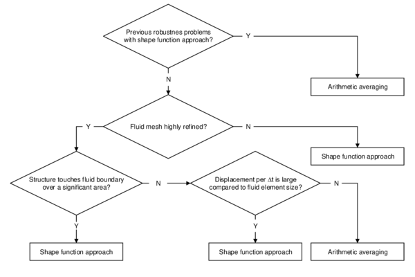
|
| Figure 199: Recommendations w.r.t. the given pressure mapping techniques - The picture categorizes the given techniques according to their proper field of application. |
As illustrated in figure 188, this is for example the case when the respective fluid element contains the structure boundary. In these cases, we chose all mapping strategies discussed before to map an equal positive and negative face pressure. This generally leads to a very conservative and robust behavior on boundaries even though we are certainly introducing errors by that. The hence introduced errors are, however, part of the intrinsic approximation errors which an embedded method comprises. Assuming a sufficiently fine mesh this approximation error on the structure boundary is negligible.
More problematic is the case when the situation of embedded structure nodes in a non-cut fluid element occurs beyond the structure boundary somewhere on the wet interface of the structure. Therefore consider the test case as depicted in figure 200 where the hull of a sphere is put into a fluid domain with assigned to all fluid nodes outside the sphere and to the ones in the interior. Here we have no clear structure boundaries but two wet surfaces, the inner and the outer. From a mapping routine we expect here that for all structure nodes a positive face pressure of and a negative face pressure of is assigned. However, when using for example the arithmetic averaging2 we get the results depicted in figure 201.
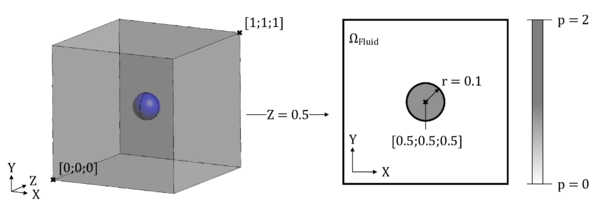
|
| Figure 200: 3D testing scenario to reveal an intrinsic mapping problem in an embedded approach - The scenario is adopted from figure 186 but has a simplified pressure distribution (constant inside and outside the sphere) |

|
| Figure 201: Results of pressure mapping for problematic intersection patterns of fluid and structure element - Both results are obtained with a refinement of: |
Even though the results generally show a correct mapping, they clearly contain an outlier in the negative face pressures. The underlying problem here gets obvious when looking at the intersection pattern at this point, which is reproduced in figure 202. A schematic sketch of this situation is given in 203. Here it can be seen that the surface of the sphere and hence one structure node enters a certain fluid element without cutting any of the latter´s edges. This means that all the nodes of the given fluid element are considered to be outside and so have a pressure of . Mapping strategies that assign positive and negative face pressure to the structure based on the information from the fluid element they are lying in, as all the strategies that do not contain neighbor search techniques, clearly have no chance here to identify the correct negative face pressure of the affected structure node since the respective fluid element does not contain any information about it. As this problem principally appears in the same form like the one discussed above for the structural boundary, i.e. we have structure nodes within a non-cut fluid element, the given pressure mapping techniques assign alternatively an equal pressure to the positive and the negative side of the structure. This, however, may lead to severe pressure gradients, as could be seen in figure 201.
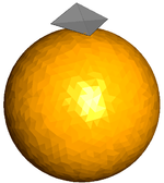
|
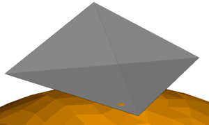
|
| (a) Overview | (b) Close up |
| Figure 202: Intersection pattern that leads to problems in pressure mapping - The grey tetrahedron represents the problematic fluid element. | |
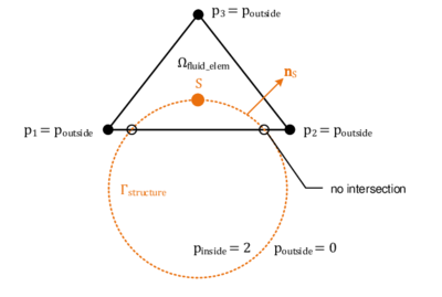
|
| Figure 203: Mapping problem due to approximation errors in the embedded approach - The figure shows a schematic sketch of the intersection pattern that yields to the bad representation of the negative face pressure in figure 201. Note that this effect arises because of indeed can be determined correctly in , but can not since there are no nodes available that contain information about here. |
As obvious with the given test example of the sphere, the problem in particular occurs for curved structures. Important to note is that, unless the fluid mesh is excessively refined, i.e. the curvature of the structure that a single fluid element recognizes becomes negligible small, this problem cannot be circumvented by a simple refinement reliably since there might be always local spots that show the situation given in figure 202 on a small scale. If such a wrong pressure assignation now happens at structure nodes that are highly transient, the simulation may get significantly unstable which may render analyses of in particular strongly coupled FSI scenarios impossible. In fact this restricted the choice of our testing examples later significantly.
The problem of sometimes being not able to assign to a structure embedded within one fluid element positive and negative face pressures alike is originated in the different kinds of intersection patterns that may arise for overlapping meshes and so is of a general nature in an embedded approach. As addressed before, one solution might be to use neighbor-search algorithms in conjunction with projection techniques to overcome this problem. Even though we will not discuss this within this work an idea shall be given in figure 204. In fact, overcoming this problem is essential for the applicability and also acceptance of the embedded method which is why developments of this kind have to be part of future projects.
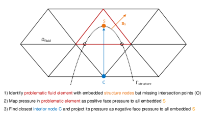
|
| Figure 204: Suggestion for a process to remedy an important mapping problem in the embedded approach |
(1) including the aforementioned three
(2) The results are the same for the other techniques
8.3.3 Velocity mapping
As already indicated in the introduction of this chapter, the velocity mapping essentially is an extrapolation of the velocity vector of an embedded structure node to the surrounding intersection nodes of the fluid element, that again expect velocity vectors. This implies tensor operations of higher order rendering the velocity mapping very expensive in general. This is one challenge. Another challenge is a correct choice of the reference velocity for the mapping. Therefore consider the case that within one fluid element several nodes from the discretization of the structure with different velocity may be embedded (see figure 205). In this case the question is, which of the embedded velocities has to be chosen as reference vector for a mapping or how do the embedded velocities have to be combined to form such a reference?
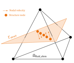
|
| Figure 205: Several structure nodes embedded in one fluid element with each having a different velocity - The picture shows a rotation of the structure around |
Both facts require intense development and implementation work which is why we will choose a solution from a more pragmatic point of view: We note that the velocity mapping is basically the practical implementation of the imposition of the velocity boundary condition in an embedded environment. The developed approach here is hence closely following the assumptions in section 2.2.4.3. Based on these assumptions, the idea is now the following.
First we take the nodal velocities of the structure nodes inside the cut fluid element and pick out only the one velocities of the structure which are given at the intersection points to the fluid element. Then we form the arithmetic average of these velocities for each fluid element separately as
|
|
(8.29) |
where is the total number of intersection points and the nodal velocities of the structure at the intersection points. This average is now considered to be the reference embedded velocity which again is assumed to be constant along the interface. For sure we are by that neglecting the fact that the velocity may vary within the fluid, but assuming a sufficiently fine mesh, this is a fair approximation and in some cases even exact. So the challenge of choosing a reference value for the embedded velocity was reduced to a simple computation of the average of the given velocities at the intersection points.
Having computed we may directly use it as velocity boundary condition on the embedded boundary in the cut fluid element. How this is done was described in 2.2.4.3. In doing so the costly tensor operation for the extrapolation of is replaced by a simple copy operation. So in total, the velocity mapping reduces to two simple steps:
- We compute as representative average of the occasionally differing velocities of an embedded structure within a cut fluid element and
- apply this vector to the surrounding intersection nodes of the cut fluid element.
An illustration of the approach is given with figure 206.
The method as described here is intentionally kept very simple and parameter free, which makes it very robust. Also in terms of its computational costs it is negligible. It remains, however, to quantify the accuracy. To measure accuracy here is more elaborate since a situation in which we know the analytic solution for the velocity profile that adjusts in the fluid as a reaction to the embedded movement with evolving time, is difficult to find. What can be done as a first step, though, is to check whether it is well implemented and in the framework of its underlying approximations not leading to any additional accuracy losses.
That this is the case could already be guessed from a qualitative point of view when we moved the embedded cylinder through a channel flow (The corresponding results were given in figure 177). In fact having observed here the different intended phenomena, i.e. a laminar flow or vortices depending on the moving direction of the cylinder, we can assume a proper mapping. It becomes, however, quantitatively more obvious when comparing the mapped nodal velocities of all cut fluid elements in this case with the imposed and known analytic velocity of the cylinder, given by equation 8.17. Denoting the mapped velocity at the fluid node in time instance as and the corresponding analytic movement of the cylinder from equation 8.17 as we can evaluate an error by means of an ordinary mean square error measure in the form:
|
|
(8.30) |
where is the total number of nodes from all the cut fluid elements in one time instance. When we depict this error over time, as done in figure 207, we can observe that there are in general no deviations from the analytic prescriptions, which is what must be expected from a velocity mapping method as described above. From that it can be concluded that the velocity mapping performs as intended and is not introducing additional accuracy losses besides the general assumption of a constant embedded velocity within all the cut fluid elements.
Indeed this is no detailed accuracy measure but rather more a function test. It is anyways evident from these investigations, that within the framework of the above introduced approximation errors we are with this velocity mapping technique capturing the general physics of the flow, especially with fine meshes. That makes the presented technique to a first, very powerful tool in the context of velocity mapping with the embedded method.
8.4 Solution examples of fully coupled problems
Having developed and discussed the single steps towards an FSI simulation, each for the body-fitted and the embedded case, we are now able to actually simulate fully coupled fluid-structure problems. The setup, simulation and final critical evaluation of two representative solution examples is topic of the present chapter. General goal of the chapter is to obtain a detailed and distinct impression of the capabilities of the embedded method.
In this context the chapter is organized in two different sections each dedicated to a single test example with a certain focus. In the first section we investigate an ultra-lightweight structure that is exposed to a fluid flow. The respective test example represents a generic abstraction of the inflatable hangar in which the main characteristics of the coupled problem are maintained. Using this example we mainly discuss applicability and performance of the embedded approach. In the second example then we focus our investigations in particular on the superior robustness. To this end we use the embedded approach to simulate flow-induced buckling of a light-weight membrane where locally extreme wrinkles occur. At last it is important to note, that the accuracy of the embedded method is not discussed in the examples. Reason therefore is the persisting problem with the pressure mapping, as it was described in chapter 8.3.2. It does not yet allow for any significant quantitative benchmarking.
Both examples are simulated in an implicit partitioned approach using an iterative Gauss-Seidel coupling strategy together with Aitken relaxation. For this reasons we do not make any attempt to distinguish between different explicit or implicit coupling strategies or do not take into account results from a monolithic approach. Moreover it is worthwhile to note that all the developments discussed in the previous chapters now resemble in these two examples. That is for instance that in an ALE simulation we use the newly developed mesh-solvers or for the partitioned analysis we make use of EMPIRE together with the developed interface. That is why the following examples are not just tests in terms of the above criteria but may also be regarded as a functional verification of all the new developments that were discussed so far.
8.4.1 An inflatable membrane in a CFD context
Within this chapter we discuss the embedded solution procedure in terms of performance and applicability. To this end we use a generic testing example that comprises a block-shaped fluid domain in which a lightweight membrane structure is embedded. The membrane itself is closed and forms a hollow half-sphere. Thus it is inflatable and encloses a certain volume within the fluid domain. The volume may increase during the inflation. The combined setup is representative for any inflatable ultra-lightweight structure in a fluid flow, such as e.g. the hangar from the introduction. The geometry of the corresponding model is described in figure 208 and the relevant material parameters are given in table 12.
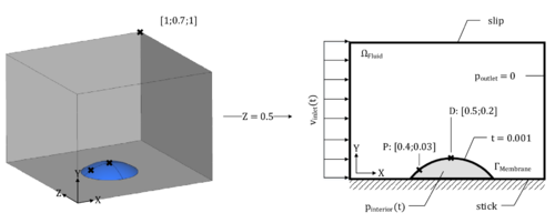
|
| Figure 208: Setup of an inflatable membrane in a CFD context |
The idea is now, that we simulate once with the ALE approach and once with the embedded approach an installation of this generic hangar within an environmental flow. Conceptually this will be realized by means of the following steps:
- After initializing a negligible environmental flow, the membrane will be inflated by applying a continuously increasing pressure field to its interior face. This will cause the membrane to expand or inflate respectively.
- After a defined time we continuously increase the velocity at the inlet of the fluid boundary which will result in a flow field that forces the structure to deflect more and more.
The corresponding boundary conditions can be found in figure 209.
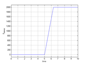
|
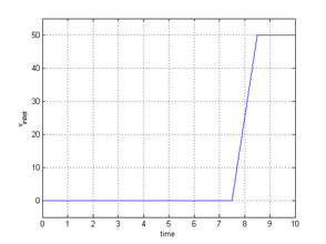
|
| (a) Prescribed inflatation of the membrane | (b) Prescribed flow |
| Figure 209: Prescribed quantities in the simplified hangar scenario | |
From a physical point of view, that is independent of the solution approach, we expect a very large deformation of the membrane both due to the inflation and because of the subsequent environmental flow. Furthermore as the flow velocity will continue to increase, the structure will be forced to technically fail at some point, which is very interesting with regards to the respective impacts in each simulation. In sum, this example is representative for a lot of possible load scenarios but nevertheless generic enough to allow for an investigation of the basic features of the applied solution method. So in the following we are able to identify key advantages as well as major drawbacks of the embedded approach, each compared to the body-fitted alternative and in view of inflatable ultra-lightweight structures.
Before discussing the simulation results, however, it is worthwhile to have a look at the different finite element models that needed to be prepared for the intended comparison. The single models are illustrated in figure 210. Without having computed anything the first and one of the most convincing advantages becomes already obvious. That is the advantage of a significantly eased pre-processing in the embedded approach. Whereas for the ALE method a detailed and explicit modeling of the interface is necessary, the embedded approach only requires a simple background fluid mesh which may be obtained very quickly by automated meshing routines. Depending on the intended level of accuracy, this may indeed contain areas with different refinement, but creating the latter is still significantly faster than an explicit modeling of the actual interface. In this context it is interesting, that the structure model may be the same in both cases, which means that for the embedded approach given models from earlier simulations may be recycled and do not have to be modeled again. This in fact is an additional advantage regarding the necessary pre-processing which might facilitate a possible change of the solution procedure from the ALE approach to the embedded approach.
After having modeled the example for both solution approaches it is each simulated for maximum . The simulation is, however, expected to fail earlier due to reasons that we will see later. In the ALE-case we furthermore want to use two different mesh-updating strategies, i.e. the Laplacian mesh-updating with adaptive conductivity and the structure-like alternative. This shall allow us to evaluate the possible improvements in more detail. For the corresponding quantitative evaluation, we are looking at the two distinct nodes that were already given in figure 208. To be more precise, we are evaluating the flow-induced displacement at node "" and the resulting pressure evolution at node "". Let us first have a look on the displacements of node in and . The corresponding results are given in figure 211 and 212, respectively.
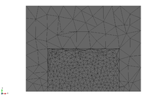
|
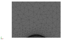
|
| (a) Fluid model in an embedded approach | (b) Fluid model in an ALE approach |

| |
| (c) Common structure model | |
| Figure 210: Possible pre-processing in the embedded and body-fitted approach | |
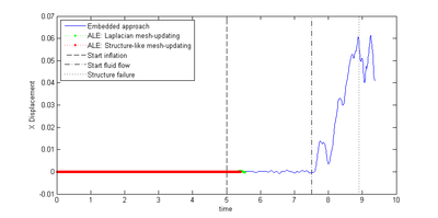
|
| Figure 211: Flow induced -movement of node from figure 208 |
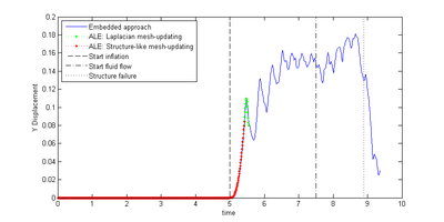
|
| (a) Over entire simulation |
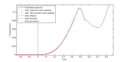
|
| (b) Close-up at failure of the ALE solution |
| Figure 212: Flow induced -movement of node from figure 208 |
First striking fact seen in both figures is, that with the embedded approach we are able to resolve a significantly wider range of movements compared to the ALE case. In particular it can be seen, that while the ALE-approach already fails1 during the inflation, the embedded approach allows to continue the simulation up to the point of the flow-induced deflection of the inflated membrane. So it is not critically influenced from the complex dynamics of the structure. Figure 213 and 214 illustrate the results from the embedded solution for two different instances in time according to the two different load stages.
As a matter of fact, when looking specifically at the -displacements given in figure 211, it can be observed that this complex dynamics is the result of a proper coupling that effectively captures the interaction in the embedded approach. That means for this example, the flow-induced load actually leads to a continuously increasing deflection in as we expected it from physics. So obviously with an embedded approach we are able to handle very large and complex movements. Furthermore we note that this is not dependent on the specific load scenario that was chosen here. We could also have defined any other load case arising for this setup, such as for example a real wind simulator instead of the given linear increase of the inflow. So in total, from a practical point of view, it can be concluded that with an embedded approach we are not just able to deal with arbitrary movements but the powerful coupling also allows various different load cases. Hence arbitrary excitation scenarios may be investigated for this kind of inflatable structures.
Second striking fact when looking at the displacement diagrams is, that changing the mesh-updating strategy in the ALE case only yields comparatively small improvements in terms of possible movements that can be simulated. This means here, that with none of the given mesh-updating strategies we were able to simulate the entire inflation together with the later deflection phase. Only the change to the embedded solution procedure really allows to overcome the respective limitations. Putting this in a more general context, one may realize that with an ALE-solution procedure there will be always a limit beyond which a proper mesh-update is not possible anymore2. So having an FSI problem where such a limit is reached, it may be very attractive to choose an embedded solution approach instead of trying various different sophisticated and possibly costly mesh-updating strategies which only allow for a certain shift of the limits instead of really overcoming them.
Third, when looking in particular at the -displacement in figure 212b it can be observed, that there in fact is a quantitative difference in the results. Assuming that the ALE-approach generally is more accurate than the embedded one, this difference may be regarded as true accuracy loss. How this accuracy loss actually influences the principle behavior of the structure and to what extend the system's dynamic is affected by that are still two open questions which could not be answered in the scope of this work. It is nevertheless interesting to note that in this example the simulated principal movement of the membrane up to the point of failure is qualitatively the same with either approach.
Apart from the movement, also the actual failure situation is interesting. Looking at the results, it can be observed, that the embedded and the ALE approach fail due to two different reasons. While the ALE approach does not come across an inappropriate mesh-update, which is a numerical problem arising from the explicit modeling of the coupling interface, the embedded approach fails because either of the single partitions, i.e. the fluid model or the structure model, fails, which is not a problem of the coupling but rather more a question of the quality of the single field models. In this example for instance, the embedded FSI approach failed because the structure simulation failed, which in turn is the consequence of invalid element formations that occur due to the fact that we are despite this large movements neglecting physical effects like self contact etc.. Figure 215 shows the corresponding failure situation of the structure model in the embedded case. The failing mesh-update in the ALE case is illustrated in figure 216.
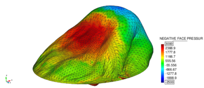
|
| Figure 215: Failure of structure model in the embedded case - The picture shows the actual structure model with mapped surface pressure at . Note the interpenetrating and overlapping elements. |
Essentially these investigations show, that in the embedded approach the coupling is truly able to deal with very complex movements and limits are mainly occurring due to the naturally limited capabilities of the single field simulations. Neglecting the still existing challenges in pressure mapping, this behavior reveals an intrinsic robustness of the embedded approach which in this form does not exist in an ALE solution. It is this robustness that in the given and other scenarios helps the FSI simulation to “survive” erratic physical behavior, which is why the embedded approach can be in fact regarded as a method to handle large and at the same time complex movements. As a matter of fact, the simulation of the entire load scenario that was planned for the given example, so the inflation and the flow-induced deflection until failure of the structure, was only possible with the embedded approach.
Apart from the displacement it is also interesting to look at the gradient of the stagnation pressure at node . The respective results are depicted in figure 217. Here mainly two things are striking. First, the shown stagnation pressure is indeed the driving force which induces the -displacement that we saw before. The steep gradient occurring right after introducing the surrounding flow corresponds to what physically can be expected. In fact when comparing the peaks along the pressure increase they perfectly match to the peaks that could be observed in the horizontal displacements given in figure 211.
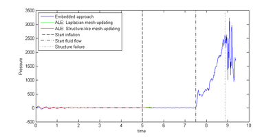
|
| Figure 217: Pressure evolution at node from figure 208 |
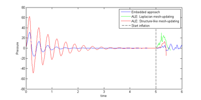
|
| Figure 218: Close-up of the pressure evolution at node from figure 208 |
Second interesting fact is revealed when looking a little closer at the pressure gradient in the beginning of the simulation as depicted in figure 218. Looking at this close-up we first note that the results in both the different solution approaches actually cannot be significantly compared since the FSI-simulation crashes, too, quickly in case of the ALE approach. A quantitative confrontation of the different solution approaches hence is not possible. Nevertheless what is interesting is the fact that in the embedded approach the flow initialization phase, where we observe a periodic converging pressure gradient, seems to be considerably quicker and also in terms of its magnitude significantly less distinct. It is obvious that this is an effect of the weak imposition of the boundary conditions at the coupling interface in the embedded approach which naturally tends to damp oscillations. This damping may also be regarded as some kind of additional robustness advantage of the embedded approach in contrast to the ALE procedure. It is, however, clear, that this numerical damping at the same time affects the accuracy of the solution.
Having now seen a few of the major advantages of the embedded approach, an important negative effect, that was encountered during the above analysis, shall be mentioned. To this end we have a look at the vertical displacement of node when the above membrane is inflated comparatively slowly. The corresponding displacement curve is depicted in figure 219. Due to the very slow inflation of the membrane we in the beginning do not get this oscillating movement as we saw it in figure 211a but rather more a steadily growing membrane after a short transient phase. Actually this is what we physically expected from a slowly inflated membrane. Nevertheless, when continuing the simulation, at around , suddenly a highly dynamic behavior forms out, which continues to grow more and more as the structure keeps inflating.
The reason for this unexpected dynamic behavior was found to be the mapping problem described in chapter 8.3.2. Due to the curved shape of the membrane locally bad intersection patterns formed out. At the corresponding spots then the actual pressure conditions could not be resolved properly which eventually influenced the system dynamics critically. This observation emphasizes the demand for a powerful and robust mapping technique since possible limitations might not necessarily lead to a crashing simulation, where we are technically able to observe a problem free of doubt. Instead they can just initiate or change the dynamic behavior which is much more subtle and hence significantly more difficult to encounter.
At this point we may summarize: Apart from any solution specific characteristics, the pre-processing turned out to be much easier for the embedded approach than for the body-fitted case. As a matter of fact it could be seen that it offers not just advantages in terms of a simplified modeling, even when introducing local refinement levels, but also allows to recycle given structure models that only have to be put into a new fluid context for an embedded FSI simulation. Regarding the actual simulation of the given weakly coupled problem it could be observed, that the embedded approach is able to resolve very complex and large movements whereas showing a very robust coupling behavior. Both characteristics together allow, in the general case of highly deforming lightweight structures exposed to a fluid flow, for the simulation of various load scenarios. The ALE formulation by contrast was not able to cope with extended movements of that kind. Also using different mesh-updating strategies only yielded small improvements in this context. So finally we may conclude: Indeed it has to be assumed that the ALE approach is more accurate. But relaxing the accuracy requirements in the embedded case such that we are able to capture the large and complex movements of this type of lightweight structures at all, turns out to be a fair solution approach because the principle deformation behavior, in which we are generally interested for this kind of problems, might be captured anyway. Nevertheless it could also be shown that even in this weakly coupled example the simulation in the embedded case can react delicately to the exclusively herein existing pressure mapping problems which emphasized the importance of further developments in this field.
(1) What failure means in either case is seen later. In all figures failure is seen as a sudden stop in the records.
(2) Assuming that an expensive re-meshing is not an alternative.
8.4.2 Flow-induced buckling of a membrane
In the previous section the embedded method was found to be very powerful in terms of arbitrary large movements of membrane structures in a CFD context. Moreover it could already be seen, that it offers particular advantages in terms of robustness. Since robustness is of major importance in simulations where ultra-lightweight structures are exposed to a fluid flow, we will in the following investigate the corresponding capabilities of the embedded method in more detail.
Firstly it is important to understand why robustness is a particular critical issue in these types of FSI scenarios. Therefore consider the case of the inflated hangar which deforms under given wind action. A respective simulation result was already shown in figure 21. Since membranes are lacking any kind of intrinsic bending or compressive stiffness it may from a physical point of view happen, that parts of the structure wrinkle or even touch themselves due to natural folding. As a matter of fact, wrinkling is a big challenge for mesh-updating procedures and hence typically leads to severe problems in a body-fitted solution approach. Folding or self-contact moreover lead in almost every case to a crashing analysis. So whatever alternative is developed to deal with large movements of ultra-lightweight structures, it has to be able to deal with these phenomena.
To see in this context the performance of the embedded method the test scenario shown in figure 220 was designed. In here there is a curved membrane positioned within a gravitation free fluid channel. The idea is now that a fluid flow is applied to the channel inlet such that the membrane is forced to buckle through towards the opposite site. One might think of a sheet of paper which is blown from one side until it buckles trough. See figure 221 for a three-dimensional impression. The scenario is similar to the one of the hangar in that sense, that we expect from physics that the membrane shows significant folds and wrinkles as it continues to move to the other site.
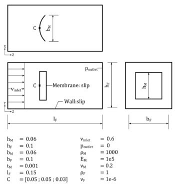
|
| Figure 220: 3D setup of the flow-induced buckling of a membrane |
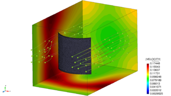
|
| Figure 221: 3D model of the flow-induced buckling of a membrane |
Knowing the physics, it is interesting now, how the solution of the given fluid-structure problem is influenced by these local, exclusively structure-related, phenomena. To this end we have a look at the displacement and pressure gradient at node (see figure 220) at . The corresponding results from the embedded approach are depicted in 222 and 223.
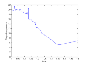
|
| Figure 222: Gradient of stagnation pressure at point from figure 220 |
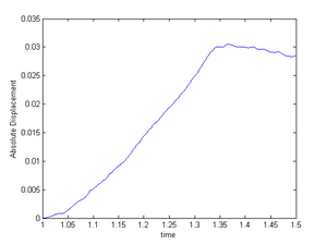
|
| Figure 223: Gradient of absolute displacement at point from figure 220 |
In both graphs we can observe in fact what physically has to be expected. That is, a stagnation pressure forms out which, when the structure is released, drops continuously in time. This is due to the fact that the membrane starts to buckle and therefore undergoes a movement, as can be seen from the displacement graph. This movement or the corresponding structural velocity, respectively, increases the dynamic pressure at point and lowers the total pressure in front of the membrane. Then, with continuing time, the membrane will be buckled through such that it effectively represents an obstacle in the fluid causing the flow to stagnate again in front of the structure. The stagnation pressure then starts to increase again.
The most important observation here is, that the results seem to be physically correct and no failure occurred, even though we had to expect wide-ranging areas of wrinkles. So obviously the embedded approach behaves very robust in such situations. To which extend, however, gets first visible when actually looking at the overall deformation during the simulation. Figure 224 illustrates the latter by means of a sequence of contour and profile plots.
Looking at the herein depicted deformation pattern, one can see that in fact the embedded approach handles the massively occurring wrinkles without any problems. So despite the complex mesh configuration of the structure, the FSI simulation remains stable without any additional loss of accuracy. Obviously, when using a body-fitted approach, this would not be the case, since a mesh-updating procedure would most probably fail at a certain instance in particular at highly transient spots with local peaks and valleys such as they appear in the middle of the membrane. One typical remedy in the latter case certainly might be a complete re-meshing. But since the wrinkles are occurring during the entire simulation a re-meshing would have to be performed in each step causing an explosion of the computational costs. Moreover, even with a re-meshing there is no guarantee that all the elements in the fluid are properly distributed. So in fact we observe a superior robustness of the embedded approach when comparing it to any body-fitted method, such as the ALE approach.
At this point it is worthwhile to recap also from the other chapters, that the herein presented embedded method poses a particularly robust method for fluid-structure interaction analysis because of three facts: Firstly there is no technical link between the different discretizations involved, which is why any mesh-update generally becomes obsolete. Nevertheless, there exists of course a coupling. Here, however, the velocities are applied in a weak sense which yields a second robustness benefit. Third and last reason is based on the fact that an embedded approach introduces implicitly a certain length-scale below which no structural detail can be resolved. The length-scale is thereby defined by the background fluid mesh. So every detail of an embedded structure which is smaller than the corresponding size of the background fluid element will not be captured. This implicitly filters problematic local effects such as wrinkles. For an impression see figure 225. It is the last reason that mainly affects the accuracy of the solution, which is why for this simulation again the earlier presented refinement strategy was applied. So in the present simulation the structure is seen by the embedded solver as shown in figure 225c.
At the end of this chapter it may be summarized: The embedded approach is not just a powerful solution procedure for FSI problems in which structures undergo large movements or show complex deformation patterns, but it poses also a significantly more robust alternative to the given body-fitted ALE approach. In fact it is the robustness, which makes it superior in cases where we have local structural phenomena like wrinkles. In these cases relaxing the accuracy requirements and by that allowing the computation of examples, which otherwise would not be solvable at all, seems to be a fair justification for the application of this alternative. Finally, taking into account also the results from the previous chapter, we may conclude: The herein presented embedded method is a powerful and robust alternative for the fluid-structure interaction analysis of ultra-lightweight structures.
9 Summary and conclusion
In the course of this monograph two state-of-the-art methods for the simulation of 3D fluid-structure interaction within the multiphysics software Kratos were further developed. Particular focus was the development of a new embedded approach, which can efficiently handle complex and large structural deformations as they occur with ultra-lightweight structures inside a fluid flow. Also a given ALE-based method was extended by several mesh-updating strategies as a basis for a comparison of both methods. The extensive comparison finally demonstrated the performance and deficits of both approaches with regard to the coupled simulation of ultra-lightweight structures.
As a basis for the embedded approach, a level set algorithm (distance function) was developed and implemented. This algorithm allows to represent any structure embedded into a tetrahedral fluid mesh robustly. Planar surfaces are thereby represented exactly, whereas curved, edged and discontinuous surfaces are approximated yielding a loss of accuracy. It could be shown, however, that the approximation error is reduced by a general fluid mesh refinement. In this context, very thin bodies turned out to be the most challenging structures since in general the resolution of the smallest geometry details that can be represented in the embedded approach strongly depend on the size of the elements in the fluid mesh. To handle such cases an adaptive mesh refinement was proposed. By means of different test cases including large scale practical examples performance and physical limits of the embedded distance function were elaborated and discussed.
Using the distance function and a discontinuous element technology developed at CIMNE, a solver based on the embedded approach was implemented and enhanced to enable fluid simulations with embedded boundaries. By means of different test scenarios a qualitative and quantitative assessment in terms of accuracy and robustness of the embedded solver was carried out. Regarding the accuracy, particularly the simulation of the Silsoe benchmark showed quantitative differences to given data from body-fitted analyses or measurements. It was found that this is due to still open limitations arising from the implementation. It was also found that the application of refinement strategies can improve the corresponding solution quality. Further investigations or implementations, however, will be a matter of future research. Apart from the solution criteria, all cases showed, as expected, a superior advantage of the embedded approach in terms of modelling, since single meshes are in here just overlapped. This turned out to be a very convenient advantage since it reduces the modelling effort to a minimum. In fact the time needed to model the tests with the embedded approach was only a fraction of the time needed to model the cases with a body-fitted approach. The more complex the example the more distinct the difference.
Approaching the partitioned simulation of fluid-structure interaction with the embedded method, the mapping of the relevant pressure and velocity fields between the interacting domains was established. Especially different routines for the efficient pressure mapping were elaborated and compared to each other towards robustness, efficiency and accuracy. Although the applied mapping algorithms turn out to be very accurate, there are structure configurations in which the mapping fails locally and might lead to serious global instabilities. However, by implementing a closest point projection, a remedy to approach this problem was proposed. This will be part of successive research.
Within the Kratos multiphysics environment we setup and run implicit simulations of simple and complex coupled fluid-structure scenarios. This was achieved by making use of the coupling software EMPIRE. An interface to EMPIRE was implemented in Kratos in order to work with the ALE-based as well as the embedded method. By that, the cooperation between the Technical University Munich and CIMNE in Barcelona was extended as this interface tool allows to use the structural solver Carat (TUM) and the fluid solver Kratos (CIMNE) in a common multiphysics framework.
A main achievement presented in this monograph was the realization of complete coupled fluid-structure simulations with the embedded approach. The artificial added-mass effect, as a typical numerical problem in partitioned FSI analyses, could be handled by means of a stabilization technique which was successfully introduced and implemented into the framework of the embedded method. In order to compare the embedded method with body-fitted approaches, the pre-implemented ALE solver in Kratos has been extended by several mesh-updating strategies that can handle large structural deformations. Based on all the aforementioned implementations, different test cases were solved in order to directly compare both formulation methods in terms of mainly robustness and performance. Here we saw a clear robustness advantage of the embedded method. At the same time it allowed for very large and complex movements during a coupled simulation making it very attractive for the simulation of ultra-lightweight structures exposed to an atmospheric environment. In fact the nice handling of folding and wrinkling phenomena even exceeded our expectations. An accuracy comparison by contrast was not possible due to numerical problems related to the above mentioned mapping failure. Rather more the problems emphasized the need for a sophisticated mapping routine which is able to handle all types of intersection patterns that may appear in an embedded model. Profound accuracy investigations and further development of the mapping routines are therefore essential in the subsequent research.
The intensive investigations throughout this monograph allow to convey the message that the embedded approach cannot replace a body-fitted approach, it rather complements it. Using a body-fitted approach, such as the ALE method, the structural geometry can be indeed represented very accurately which allows to conduct FSI simulations in which even boundary layer flows can be considered. For the treatment of ultra light-weight structure, though, the ALE method may fail even with the furthest developed mesh-updating strategy. In such cases the embedded approach provides a solution. Although the geometry representation of the embedded method is by construction worse, it can handle arbitrarily complex shapes or movements which in fact may render this method the only option available. Obtaining a reasonable accuracy for very complex shapes under severe deformations with reasonable computational effort shapes is, however, still a challenge. A possible solution therefore might be the a combination of the embedded and body-fitted approach to a Chimera technique. This again will be part of future projects.
References
[1] Solar Impulse. (2013) "http://www.solarimpulse.com/"
[2] Lawrence E. Malvern. (1969) "Introduction to the Mechanics of a Continuous Medium". Prentice-Hall 138-143
[3] J. Donea and A. Huerta. (2003) "Finite Element Methods for Flow Problems". John Wiley & Sons 4-32
[4] Y. Cengel and J. Cimbala. (2006) "Fluid Mechanics Fundamentals and Applications". McGraw-Hill 122-128
[5] J. Donea and A. Huerta and J.-P. Ponthot and A. Rodríguez-Ferran. (2004) "Arbitrary Lagrangian-Eulerian Methods", Volume 1. Encyclopedia of Computational Mechanics 413-437
[6] R. Rossi. (2006) "Light-weight Structures. Numerical Analysis and Coupling Issues". Universita degli Studi di Bologna
[7] R. Codina. (2001) "Pressure Stability in Fractional Step Finite Element Methods for Incompressible Flows", Volume 170. Journal of Computational Physics 112-140
[8] R. Codina and O. Soto. (2004) "Approximation of the incompressible Navier–Stokes equations using orthogonal subscale stabilization and pressure segregation on anisotropic finite element meshes", Volume 193. Computer Methods in Applied Mechanics and Engineering 1403-1419
[9] J.C. Butcher. (2008) "Numerical Methods for Ordinary Differential Equations". John Wiley & Sons, 2nd Edition
[10] R. F. Ausas and F. S. Sousa and G. C. Buscaglia. (2010) "An improved finite element space for discontinuous pressures", Volume 199. Computer Methods in Applied Mechanics and Engineering 1019-1031
[11] G. A. Holzapfel. (2000) "Nonlinear Solid Mechanics. A Continuum Approach for Engineering.". John Wiley & Sons Ltd., Chichester
[12] T. Belytschko and W. K. Liu, B. Moran, K. Elkhodary. (2000) "Nonlinear Finite Elements for Continua and Structures". John Wiley & Sons
[13] O.C. Zienkiewicz and R. L. Taylor and J.Z. Zhu. (2005) "The Finite Element Method: Its Basis and Fundamentals". Elsevier Butterworth-Heinemann
[14] W. L. Wood and M. Bossak and O. C. Zienkiewicz. (1980) "An alpha modification of Newmark's method", Volume 15. International Journal for Numerical Methods in Engineering 10 1562-1566
[15] N. M. Newmark. (1959) "A Method of Computation for Structural Dynamics", Volume 85. Journal of Engineering Mechanics 67-94
[16] A. Gerstenberger. (2010) "An XFEM based fixed-grid approach to fluid-structure interaction". Technische Universität München
[17] G. Hou and J. Wang and A. Layton. (2012) "Numerical Methods for Fluid-Structure Interaction - A Review", Volume 12. Communications in Computational Physics 337-377
[18] R. van Loon and P.D. Anderson and F.N. van de Vosse and S.J. Sherwin. (2007) "Comparison of various fluid-structure interaction methods for deformable bodies", Volume 85. Computers & Structures 11-14 833 - 843
[19] T. J. Hughes and W. K. Liu and T. Zimmermann. (1981) "Lagrangian-Eulerian finite element formulation for incompressible viscous flows", Volume 29. Computer Methods in Applied Mechanics and Engineering 3 329-349
[20] M. A. Puso. (2004) "A 3D mortar method for solid mechanics", Volume 59. International Journal for Numerical Methods in Engineering 3 315-336
[21] C.S. Peskin. (1977) "Numerical analysis of blood flow in the heart", Volume 25. Journal of Computational Physics 3 220-252
[22] C.S. Peskin. (2002) "The immersed boundary method", Volume 11. Acta Numerica 479-517
[23] L. Zhang and A. Gerstenberger and X. Wang and W.K. Liu. (2004) "Immersed finite element method", Volume 193. Computer Methods in Applied Mechanics and Engineering 21 2015-2067.
[24] R. Glowinski and T.-W. Pan and J. Periaux. (1997) "A Lagrange multiplier/fictitious domain method for the numerical simulation of incompressible viscous flow around moving rigid bodies: (I) case where the rigid body motions are known a priori", Volume 324. Comptes Rendus de l'Academie des Sciences - Series I - Mathematics 3 361-369
[25] X. Wang. (2006) "From Immersed Boundary Method to Immersed Continuum Method", Volume 4. International Journal for Multiscale Computational Engineering 1 127-145
[26] R. Mittal and G. Iaccarino. (2005) "Immersed boundary methods", Volume 37. Annual Review of Fluid Mechanics 239-261
[27] P. Gamnitzer and W.A. Wall. (2006) "An Ale-Chimera method for large deformation fluid structure interaction". Proceedings European Conference on Computational Fluid Dynamics CD550
[28] C. Farhat and C. Degand and B. Koobus and M. Lesoinne. (1998) "Torsional springs for two-dimensional dynamic unstructured fluid meshes", Volume 163. Computer Methods in Applied Mechanics and Engineering 231-245
[29] T. J. Baker. (2003) "Mesh deformation and modification for time dependent problems", Volume 43. John Wiley & Sons. International Journal for Numerical Methods in Fluids 6-7 747-768
[30] A.M. Winslow. (1963) "Equipotential Zoning of Two-dimensional Meshes", Volume 1. Journal of Computational Physics 149-172
[31] R. Wüchner. (2006) "Mechanik und Numerik der Formfindung und Fluid-Struktur-Interaktion von Membrantragwerken". Technische Universität München
[32] U. Küttler and W.A. Wall. (2008) "Fixed-point fluid-structure interaction solvers with dynamic relaxation", Volume 43. Computational Mechanics. Springer. Computational Mechanics 1 61-72
[33] U. Küttler. (2009) "Effiziente Lösungsverfahren für Fluid-Struktur-Interaktions-Probleme". Technische Universität München
[34] C. A. Felippa and K. C. Park. (2005) "Synthesis Tools for Structural Dynamics and Partitioned Analysis of Coupled Systems", Volume 3. Engineering Structures under Extreme Conditions 50-111
[35] C. E. Brennen. (1982) "A review of added mass and fluid inertial forces". Naval Civil Engineering Laboratory, Port Hueneme, Carlfornia 1-16
[36] C. T. Crowe and J.D. Schwarzkopf and M. Sommerfeld and Y. Tsuji. (1997) "Multiphase flows with droplets and particles", Volume 1. CRC Press. CRC Press 81-86
[37] P. Causin and J.F. Gerbeau and F. Nobile. (2005) "Added-mass effect in the design of partitioned algorithms for fluid-structure problems", Volume 194. Computer Methods in Applied Mechanics and Engineering 42-44 4506-4527
[38] S. R. Idelsohn and F. Del Pin R. Rossi and E. Oñate. (2009) "Fluid-structure interaction problems with strong added-mass effect", Volume 80. John Wiley & Sons, Ltd. International Journal for Numerical Methods in Engineering 10 1261–1294
[39] G. Steber. (2012) "Evaluation of the finite element method for turbulent flows with the open source software Kratos". Technische Universität München
[40] S. Turek and J. Hron. (2006) "Proposal for Numerical Benchmarking of Fluid-Structure Interaction between an Elastic Object and Laminar Incompressible Flow", Volume 53. Fluid-Structure Interaction. Springer Berlin Heidelberg 371-385
[41] M. J. Quinn. (2003) "Parallel Programming in C with MPI and OpenMP". McGraw-Hill Education Group 43-49; 93-96; 404-410
[42] P. Dadvand and R. Rossi and M. Gil and X. Martorell and J. Cotela and E. Juanpere and S.R. Idelsohn and E. Oñate. (2013) "Migration of a generic multi-physics framework to HPC environments", Volume 80. Computers & Fluids 0 301-309
[43] R.-P. Mundani. (2012) "Master level course: Parallel Computing". Chair for Computation in Engineering, Technische Universität München
[44] X.-H. Sun and D.T. Rover. (1994) "Scalability of Parallel Algorithm-Machine Combinations", Volume 5. IEEE Transactions on Parallel and Distributed System 6 599-613
[45] X. Zhang and Y. Yan, Q. Ma. (1994) "Measuring and Analyzing Parallel Computing Scalability", Volume 2. International Conference on Parallel Processing 295 - 303
[46] S. F. Frisken and R. N. Perry. (2002) "Simple and efficient traversal methods for quadtrees and octrees", Volume 7. Journal of Graphics Tools 2002
[47] T. Akenine-Möller. (2001) "Fast 3D Triangle-Box Overlap Testing", Volume 6. Journal of Graphics Tools 29-33
[48] J. Zudrop. (2013) "http://www.jenszudrop.de/gallery-videos/"
[49] P. Dadvand and R. Rossi and E. Oñate. (2010) "An Object-oriented Environment for Developing Finite Element Codes for Multi-disciplinary Applications", Volume 17. Archives of Computational Methods in Engineering 3 253-297
[50] T. Wang and S. Sicklinger and R. Wüchner and K.-U. Bletzinger. (2013) "Concept and Realization of Coupling Software EMPIRE in Multi-Physics Co-Simulation". Computational Methods in Marine Engineering 289-298
[51] T. Möller and B. Trumbore. (1997) "Fast, Minimum Storage Ray/Triangle Intersection", Volume 2. Journal of Graphics Tools. Journal of Graphiics Tools 1 21-28
[52] C. Felippa. (2013) "Master level course: Introduction to Finite Element Methods". Department of Aerospace Engineering Sciences, University of Colorado at Boulder
[53] R. Rossi and J. Cotela and N.M. Lafontaine and P. Dadvand and S.R. Idelsohn. (2013) "Parallel adaptive mesh refinement for incompressible flow problems", Volume 80. Computers & Fluids 10 342-355
[54] P.J. Richards and R.P. Hoxey and L.J. Short. (2001) "Wind pressures on a 6m cube", Volume 89. Journal of Wind Engineering and Industrial Aerodynamics 14-15 1553–1564
[55] Robert D. Blevins. (1990 (Reprint 2001)) "Flow-induced vibrations". Krieger Publishing Company, 2nd Edition
[56] G. B. Wright. (2003) "Radial Basis Function Interpolation: Numerical and Analytical Developments". University of Colorado
[57] B. J. Charles Baxter. (1992) "The Interpolation Theory of Radial Basis Functions". Cambridge University
[58] D. Straub. (2012) "Master level course: Risk Analysis 1". Engineering Risk Analysis Group, Technische Universität München F1 - F25
Document information
Published on 01/01/2015
DOI: 10.13140/RG.2.1.1079.8561
Licence: CC BY-NC-SA license
Share this document
claim authorship
Are you one of the authors of this document?
