(Created page with "<!-- metadata commented in wiki content <div class="center" style="width: auto; margin-left: auto; margin-right: auto;"> <big>'''Interpretation of dam monitoring data combin...") |
m (Andre moved page Draft Conde 559842996 to F. et al 2019a) |
(No difference)
| |
Revision as of 20:00, 5 May 2020
Abstract: The installation of automatic data acquisition systems, together with the use of machine learning, allow obtaining useful information on the behaviour of dams. In this contribution, an example of application for a machine learning based predictive model is presented. Specifically, the level in a piezometer and its association with the reservoir level is studied for an embankment dam. The results show the model's ability to identify changes in dam response by taking full advantage of the available monitoring data. The flexibility of the algorithm allows different types of variables to be analysed without the need to determine a priori which are the most influential loads or how they affect the target value. The model has been implemented in a software tool that includes additional functionalities, specific for the treatment and exploration of dam monitoring data. It can be applied to different dam types and response variables.
Keywords: Machine Learning, Boosted Regression Trees, Data Analysis, Data Exploration, Embankment Dam.
1 Introduction
With the implementation of automatic monitoring and data acquisition systems, databases of increasing size are generated for dam behaviour, which can be very useful in the analysis of the response as well as in safety management. However, this increase in the volume of available data also presents challenges in terms of data analysis and processing tools, as well as methods for generating predictive models.
Traditionally, the representation of dam monitoring data has been limited to conventional spreadsheets, which was sufficient when manual data with low reading frequency were handled. The safety evaluation was based fundamentally on the expert analysis of graphs showing the evolution of the most relevant variables, as well as their relationship to the main loads, which in most of the dams are limited to the reservoir level and temperature.
In other fields of science and engineering, where large databases are available, tools are being developed to extract information from the data. These tools include highly customizable and interactive visualisation environments, which allow data to be presented in different formats, so that certain patterns and erroneous data can be identified. On the other hand, it is possible to generate data-based prediction models using machine learning algorithms that offer relevant advantages over traditional statistical methods.
VERBUND, in its digitalization process, is implementing tools of this type to extract information from the behaviour of its main dams, which already have automatic data acquisition systems. This contribution presents the result of the collaboration with CIMNE in the development of a software tool for this purpose, as well as an example of application to the Eberlaste embankment dam.
2 Case study
2.1 Eberlaste Dam
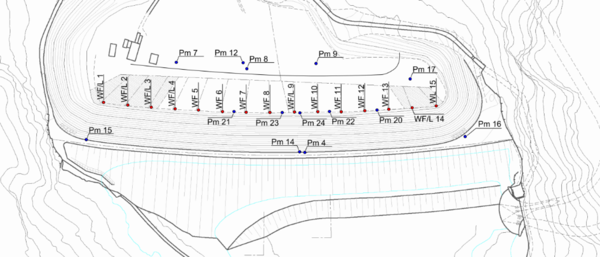
Eberlaste is an embankment dam with an asphalt concrete core and a cut-off wall as underground sealing that was completed in 1968, with a maximum height of 28 m and a crest length of 480 m. The foundation is a deep, heterogeneous, alluvial deposit. Although bedrock was found close to the surface at the abutments, the upper surface of such competent foundation features high slope towards the valley, where only river-deposited gravel and sands were found in a 125 m deep drill [1]. As a result, large settlements and relevant seepage were expected already in the design stage. A 50 m long stabilising berm was also built in the dam foreland to improve safety against ground failure [2]. The monitoring system was also designed according to these unconventional features. As such, 15 relief wells of 25 cm pipe diameter were installed, 60 m deep, at the downstream dam toe. All of them are artesian wells and the discharge is monitored continuously. 14 automated monitored and 13 manually measured piezometers allow measuring the pore water pressure in various depths. A plan view of the dam is included in Fig. 1, with the location of the monitoring devices considered.
|
In this work the data from the automated devices, which include discharge at 14 relief wells, the total seepage flow, hydraulic head at 7 of them, 14 piezometers, suspended solids (mg/l), reservoir level, air temperature, snowfall and three records of rainfall (at three different stations) are used.
With regard to the location within the dam body, the devices can be classified in three groups:
1. At the dam crest, right behind the asphalt core and the cut-off: piezometers 1,2,4-6,13-16,18,19.
2. At the downstream dam toe: Piezometers 20-24, relief wells (all)
3. At the downstream end of the berm: Piezometers 7,8,9,12,17
4. The remaining devices are sparsely located: piezometers 10 and 11 are 100 and 200 m away from the berm toe, respectively.
2.2 Data analysis process
The analysis of the monitoring data was performed with a methodology including the following steps for each output variable:
1. Exploration of the time evolution and its relation to reservoir level with the time series plots and scatterplots.
2. Fitting of a predictive model based on boosted regression trees (BRT).
3. Interpretation of the model in terms of the most influential inputs and the nature of their effect on the variable under consideration
The process is illustrated with the description of its application to Pm14 (level at piezometer #14).
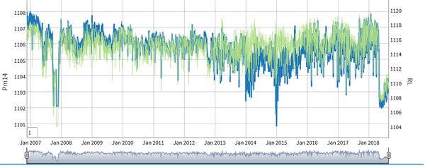
Exploration. The time series plot of the output variable, together with the reservoir level, is shown in Fig. 2. Pm 14 is displayed on the left vertical axis and the reservoir level (RL) on the right vertical axis. A possible change in dam response can be seen, since Pm14 appears above RL before 2010, then both series roughly overlap until 2014, and finally RL is above from that year on.
|
From the exploration of the time series, it is possible to identify the existence of reading errors or missing data periods. A specific functionality was developed to interactively correct these imperfections by selecting erroneous data or periods without data and replace them with interpolated values.
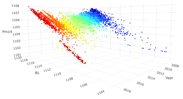
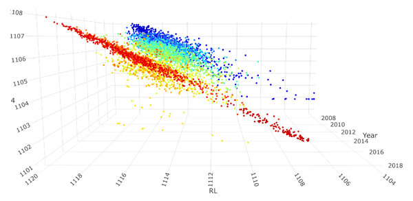
The relation between RL and Pm14, as well as its evolution over time, can be best observed in a scatterplot. This graph has functionalities to rotate the axes and zoom, for a better analysis. Fig. 3 shows two viewpoints of the data recorded for Pm14, as a function of the date and the reservoir level.
The application allows tuning the colour of the points as a function of some of the variables in the data set. Here, we used “Year” for the colours. It should be noted that “Year” variable is generated as numeric (with two decimal positions), not as integer.
This visualisation suggests that Pm14 responds linearly to RL for the most recent period (red points). The dots show higher scatter for the initial years (in blue) and appear above the straight alignment of red points. This means that Pm14 was more closely connected to the reservoir in 2007. Green points (around 2012) are closer to the more recent records.
Of course, although RL is expected to be the most influential input, Pm14 can in principle be dependent on other input variables. If that is the case, this interpretation of the scatterplot regarding the evolution over time might be wrong. This can be investigated by machine learning and the application developed.
|

|
|
Fig. 3. Different views of the 3D scatterplot of Pm14 as a function of reservoir level (RL) and date (Year).
Model fitting. Data exploration can provide interesting information, especially if the right tools are available and the task is carried out by dam engineering technicians with high knowledge on the dam under study. However, dam behaviour is often complex, and the acting loads are correlated, which makes it nearly impossible to identify certain effects by simply observing the data.
It is common to use statistical models to generate predictions of certain dam response variables and to analyse the contribution of each of the acting loads. The most commonly used example is the HST model, developed for the study of displacements in concrete dams [3]. It is based on the hypothesis that these displacements are the result of the combination of the effect of hydrostatic load, temperature and time (which includes irreversible deformations of different origin). This method has often been used both in professional practice and at the research level, although its limitations have also been identified [4].
A good number of alternatives have been proposed to overcome these limitations of HST: It does not consider the actual temperature, does not adapt well to variables other than the displacements of concrete dams, and does not allow consideration of the correlation between loads (as is the case with temperature, which is affected by the level of the reservoir). These methodologies range from advanced statistical models (e.g. HST-Grad [5], hybrid [6]) to machine learning models, which are constructed exclusively from the data (e.g. Neural Networks [7,8]).
In this work, we make use of Boosted Regression Trees (BRT), a machine learning algorithm that was the most advantageous in a comparative study [9] and which was already used for the analysis of the behaviour of an arch dam [10].
The main features of this algorithm making it appropriate for this problem are the following:
1. It allows considering variables of different nature and range of variation without the need of additional transformations.
2. It automatically selects the most relevant variables in the dam response and discards those with little influence. Hence, variable selection is not necessary.
3. It is robust when it comes to training parameters, unlike other machine learning models that require in-depth knowledge of the algorithm to carefully select model fit options.
The next step is the building of a predictive model for the output variable. As input all the available variables corresponding to the loads which might be influential on the response are considered: reservoir level, temperature, rainfall and snow, as well as the corresponding derived variables (moving average or cumulative sum, which need to be previously generated) and the time effect, which we encoded in the “Year” variable. In this example, we created moving averages and cumulative sums for 2, 7, 15, 30 and 60 days. Temperature was included to verify that the model indeed discards automatically those variables without influence on the response.
The interface allows selecting some training parameters, though the default values usually provide good results. The main decision to be made in this step is the selection of the training period, i.e. the data that will be used for model fitting. The complementary period is reserved for validation. This is important to control overfitting.
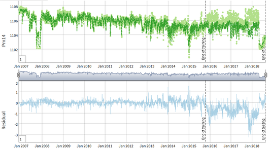
The results with default parameters show an increase in predictive error for the validation period (Fig. 4). This might be due to overfitting, or to a change in the behaviour of the response for the most recent period compared to that used for model fitting.
|
Fig. 4. Results of model fitting for Pm14 and default parameters. Mean absolute error (MAE) increases from the training set (0.2) to the testing set (0.77). This and the evolution of the residual (bottom) depict changes in the response variable for the test period
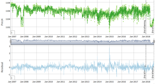
If a new model is fitted with an extended training period, till the end of 2017, testing accuracy increases (Fig. 5). This confirms that some change occurred in the response of Pm14 to the variation of the hydraulic load between 2015 and 2017. Additional verification can be obtained from the model interpretation as described in the next subsection.
|
Fig. 5. Results of model fitting for Pm14 with extended training period. Accuracy is higher for the testing period (MAE=0.23), and residual more stable.
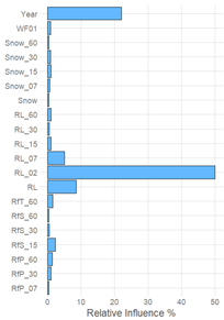
Model interpretation. The first result of model interpretation is the identification of the most influential variables, i.e. those inputs with stronger association with the analysed response. Fig. 6 shows that the moving average of two days of the reservoir level is the most influential input, followed by the time.
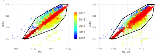
As expected, reservoir level is the most influential variable in the piezometric level considered. However, the two-days moving average shows higher importance than the raw (actual) level. This result can be verified going back to the scatterplot. Fig. 7 shows the relation between Pm14 and both RL and RL_02. A polygon was overdrawn to better observe that indeed there is less scatter of Pm14 in the RL_02 plot. This means that the association is stronger, as identified by the BRT model. This can reveal some inertia in the response of Pm14 to changes in the reservoir level.
|
|
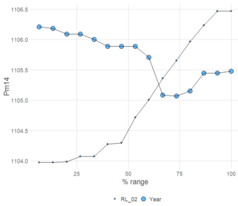
Fig. 6. Model interpretation. Left: Relative influence of the inputs considered. Right: Partial dependence of Pm14 on the two most influential variables
|
Fig. 7. Scatterplot of Pm14 as a function of RL (left) and RL_02 (right). The same polygon was superimposed to better observe that there is slightly less overall scatter for RL_02, although the correlation seems to be stronger for RL in the most recent period (red dots)
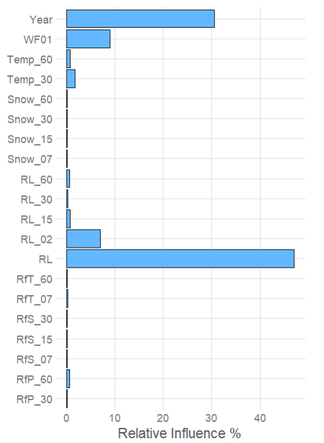
Fig. 7 also shows that there seems to be higher influence of RL for the most recent period (red dots). To verify, if the algorithm is capable of identifying this effect, a new model was fitted taking the period 2015/01/01-2017/12/31 for training. The results of the interpretation of this model for the relative influence (Fig. 8) are in agreement with the visualisation of the scatterplot: The reservoir level at the day of the reading (RL) is more relevant in this case than the two-days moving average (RL_02).
|
Fig. 8. Relative influence of input variables for a BRT model fitted with 2015-2017 as the training period. RL is the most influential variable, in accordance with the visual impression from the scatterplot (Fig. 7).
Two conclusions can be drawn from these results:
1. The relative influence computed by the software accounts for the interaction between inputs: a small difference between RL and RL_02 results in a high difference in importance, as computed by the model. This shows the capability of the algorithm for dealing with highly correlated inputs.
2. The interpretation of the BRT model allows identifying effects which are hard to detect by data exploration, even if advanced visualization tools are employed.
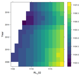
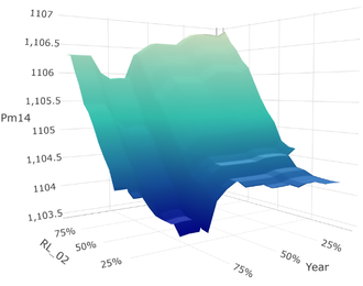
As for the time effect, the partial dependence plot shows sharp changes in the response along time (Fig. 8 right). This result is obtained for all the values of the reservoir level, as observed in Fig. 9, where the combined average effect of reservoir level and time is depicted.
|
|
Fig. 9. Combined partial dependence of Pm14 on RL_02 and time. The influence of time is nearly stable for all values of the hydrostatic load.
The effect of the hydraulic load is conventional: Positive correlation is observed, with a slope change around 1110 m.a.s.l. As regards time, there is a decrease until 2014, followed by a two-year stable period and a sharp increase around the end of 2015. These sudden changes are consistent with the operation report of the piezometer. The second was probably due to the piezometer flush performed in November 2015.
3 Discussion
Prediction models based on BRT can be useful for interpreting the behaviour of dams by analysing the monitoring data. They have the advantage of being very flexible in terms of the nature of the dam response to be analysed, as well as in terms of the amount of input data. Previous studies resulted in a good prediction capacity, as well as robustness to training parameters, which means that it is not necessary to have in-depth knowledge of the method for its practical use.
The model has a fundamental limitation that must always be taken into account: Its results, when making predictions outside the range of training data, are not reliable. This implies, for example, that the model prediction will be poor for a higher reservoir level than the historical maximum recorded in the dam. In order to control this extrapolation effect, the software developed verifies whether the test data are within the training range, and issues a warning in case of extrapolation.
The implication of this feature to the time effect has another interpretation: In this type of analysis, it is common to fit a model to the historical behaviour of the dam and apply it to analyse the current or future response of the structure. This necessarily implies extrapolating in terms of the time variable. Therefore, according to the above, the prediction would not be reliable. However, the BRT model has the particularity that in these cases it applies a constant time effect, equal to that identified in the most recent period. Therefore, a sudden increase in the discrepancy between prediction and observation reflects a change in behaviour of the variable under consideration with respect to that at the end of the training period. This can be useful for anomaly detection.
As a result, BRT models can be used for both, to identify changes in the behaviour of output variables, when analysing past behaviour (back analysis) and to detect deviations from normal performance, when applied to real-time data. In this sense, the flexibility of the algorithm allows capturing any kind of time effect without the need to make a trial and error process with functions of different shape, as is the case with conventional polynomial fitting. In the case study presented, the effect of time shows the changes in the association between the hydraulic load and the piezometric level which indeed occurs when some major action is performed on the well, such as cleaning or readjustment (as was the case in the analysed device, according to the reports). This implies sharp changes in the time effect which would have been difficult to reproduce with a combination of functions to be defined a priori.
The example shown demonstrates the flexibility of BRT models to predict variables of different nature than displacements in concrete dams, for which HST was developed and is often used. In this regard, BRT also provided useful results in terms of prediction and interpretation for other kind of variables such as leakage flow in arch dams [11], or seepage and flow at relief wells in embankment dams.
4 Summary and conclusions
A software tool for dam monitoring data analysis and interpretation was presented, with an example of application. It includes functionalities for data exploration, with high degree of interactivity. Different kinds of scatterplots and time series plots can be generated and analysed. Also, wrong data can be fixed on the fly, in the same environment.
In addition, it includes an implementation of BRT models which can be used for predicting response variables of different nature, thus extracting high degree of information from the available data. These models can be analysed to explore the degree of association between the inputs considered and the output under analysis, as well as the shape of each partial dependence. The flexibility of the algorithm results in the automatic exclusion of low relevant inputs without the need for specific variable selection. Furthermore, input effects of irregular shape can be captured by the model, as those due to modifications in the recording device. Again, this can be obtained without any specific preliminary operation or decision by the user.
The software tool can be used for different dam types and output variables, as far as adequate monitoring data are available and the results are interpreted by experienced dam engineers.
5 Acknowledgements
The authors acknowledge the financial support to CIMNE via the CERCA Programme/Generalitat the Catalunya. This work was also partially funded by the Spanish Ministry of Science, Innovation and Universities (Ministerio de Ciencia, Innovación y Universidades) through the project TRISTAN (RTI2018-094785-B-I00).
References
- 1. Hoeg, K, Valstad, T., Hansteen, O.E.: Transverse cracking in embankment dams. A literature review and finite element study. Norwegian Geotechnical Institute (1995).
- 2. ATCOLD-Austrian National Committee on Large Dams: Pumped storage hydropower in Austria (2018).
- 3. Willm and Beaujoint: ‘Les méthodes de surveillance des barrages au service de la production hydraulique d’Electricité de France, problèmes anciens et solutions nouvelles’, in IXth International Congress on Large Dams. Istanbul, pp. 529–550. (In French) (1967)
- 4. Salazar, F., Morán, R., Toledo, M. Á., & Oñate, E.: Data-based models for the prediction of dam behaviour: a review and some methodological considerations. Archives of computational methods in engineering, 24(1), 1-21 (2017).
- 5. Tatin, M., Briffaut, M., Dufour, F., Simon, A., & Fabre, J. P.: Thermal displacements of concrete dams: Accounting for water temperature in statistical models. Engineering Structures, 91, 26-39 (2015).
- 6. Perner, F. & Obernuber, P.: Analysis of arch dam deformations. 2nd International conference for long term behaviour of dams. Graz (2009).
- 7. De Granrut, M., Simon, A., & Dias, D.: Artificial neural networks for the interpretation of piezometric levels at the rock-concrete interface of arch dams. Engineering Structures, 178, 616-634 (2019).
- 8. Mata, J.: Interpretation of concrete dam behaviour with artificial neural network and multiple linear regression models. Engineering Structures, 33(3), 903-910 (2011).
- 9. Salazar, F., Toledo, M. A., Oñate, E., & Morán, R.: An empirical comparison of machine learning techniques for dam behaviour modelling. Structural Safety, 56, 9-17 (2015).
- 10. Salazar, F, Toledo, MÁ, González, JM, Oñate, E.: Early detection of anomalies in dam performance: A methodology based on boosted regression trees. Struct Control Health Monit. 2017; 24:e2012. https://doi.org/10.1002/stc. 2012
- 11. Salazar, F., Toledo, M. Á., Oñate, E., & Suárez, B.: Interpretation of dam deformation and leakage with boosted regression trees. Engineering Structures, 119, 230-251 (2016).
Document information
Published on 01/01/2019
Licence: CC BY-NC-SA license
Share this document
Keywords
claim authorship
Are you one of the authors of this document?