Quality Control and Analysis of Global Gauge-Based Daily Precipitation Dataset from 1980 to 2009

Abstract

A series of quality control (QC) procedures were performed on a gauge-based global daily precipitation dataset from the Global Telecommunication System (GTS) for the period 1980–2009. A new global daily precipitation (NGDP) dataset was constructed by applying those QC procedures to eliminate erroneous records. The NGDP dataset was evaluated using the NOAA Climate Prediction Center Merged Analysis of Precipitation (CMAP) and the Global Precipitation Climatology Project (GPCP) precipitation datasets. The results showed that the frequency distribution and spatial distribution pattern of NGDP had a nice match with those from the CMAP and GPCP datasets. The global mean correlation coefficients with the CMAP and GPCP data increased from 0.24 for original GTS precipitation data to about 0.70 for NGDP data. Correspondingly, the root mean square errors (RMSE) decreased from 12 mm per day to 1 mm per day. The interannual variabilities of NGDP monthly precipitation are consistent with the CMAP and GPCP datasets in Asia. Meanwhile, the seasonal variabilities for most land areas on the Earth of NGDP dataset are also consistent with the CMAP and GPCP precipitation products.

Keywords

global surface weather report data ; GTS data ; daily precipitation ; quality control

1. Introduction

Precipitation is a key state variable in climate and climate change researches. Both the NOAA Climate Prediction Center Merged Analysis of Precipitation (CMAP) and the Global Precipitation Climatology Project (GPCP) produce complete global precipitation datasets, which have been widely used in climate monitoring and climate change evaluation [ Xie and Arkin, 1997 , Adler et al., 2003  and Huffman et al., 1997 ]. Because the CMAP and GPCP precipitation products are not real-time and with low temporal resolution (monthly), it is difficult for them to meet the needs of climate service and climate change research operations in China which require near real-time global daily precipitation data.

The global surface synoptic dataset was extracted from the Global Telecommunication System (GTS) synoptic weather reports archived at the National Meteorological Information Center of China Meteorological Administration (CMA). This dataset includes realtime and past weather records, and covers the period from 1980 to present. It contains observations of all the major meteorological variables, providing global observations for climate service and climate change research operation in China [ Zhang et al., 2004 ]. However, due to errors in observing, entering, code transmission, and other aspects of data collection, the overall quality of the original GTS dataset was poor. Many quality control (QC) checks need to be conducted before this dataset can be used in operational climate researches.

So far, QC research was performed only on state variables with small temporal and spatial variabilities (e.g., temperature and pressure) in this GTS dataset [ Wang et al., 2006 ]. For precipitation variable, no comprehensive QC checks have been done at present. In order to meet the needs of operational application of near real-time global daily precipitation, this study focuses on applying and testing a series of QC procedures for the GTS daily precipitation data. The constructed new global daily precipitation (NGDP) dataset will also be tested and evaluated by comparing with the CMAP and GPCP precipitation products. The authors hope that this NGDP dataset can provide reliable global gauge-based daily precipitation data for operational climate monitoring and climate change researches in China in the future.

2. Data

The global surface synoptic dataset used in this study was extracted from the real-time GTS synoptic weather reports of the National Meteorological Information Center [ Zhang et al., 2004 ]. The dataset used in this study covers the period from January 1980 to December 2009, with missing data from January to June in 2000 due to the replacement of GTS receiving system at that time. There are more than 15,000 fixed land and island transmitter stations in the dataset, but about 4,000–7,000 stations have weather reports at any given month. Precipitation variables in this dataset include: 1-hour, 3-hour, 6-hour, 12-hour, and daily rainfall. In this study, QC checks are focused on daily rainfall. The CMAP monthly precipitation analysis products [ Xie and Arkin, 1997 ] and the GPCP satellite gauge combined precipitation products [ Adler et al., 2003 ] are served as validation datasets. Both datasets are monthly and cover the same period as the GTS dataset, and the horizontal resolution is 2.5° × 2.5°.

3. QC procedures

The following five steps of QC procedures are based on widely used QC methods in the world [ Eischeid et al., 1995 , Lanzante, 1996 , Wolter, 1997 , Ren and Zhai, 1998 , Harmel et al., 2002 , Hubbard et al., 2005 , Kunkel et al., 2005 , Liu et al., 2006 , Liljegren et al., 2009  and Tao et al., 2009 ]. Outliers of daily precipitation from January 1980 to December 2009 GTS dataset are removed.

(1) Duplication station check. This step addresses the replication erroneous values in the processes of data entering and transmission [ Kunkel et al., 1998 ], including station location errors, station relocation, erroneous zeros, and multiple missing value errors.

(2) Internal consistency check. This step tests violations of logical relationship between daily precipitation and daily accumulative hourly precipitation (e.g., 3-hour and 6-hour precipitation) [ Graybeal et al., 2004 ]. The total amount of precipitation in a certain day should be the maximum value of daily accumulation of observed hourly precipitation with complete record.

(3) Extreme value check. This step identifies invalid values that fall outside the range of reported world records. The global maximum and minimum daily precipitations are respectively 1,828.8 mm and 0.0 mm, which are defined and updated by the World Meteorological Organization World Weather/Climate Extremes Archive [ Lanzante , 1996 ].

(4) Temporal consistency check. It includes two steps: a) The reference standard deviation (STD) method is used to identify outliers which exceed the reasonable variation range of daily precipitation record [ Eischeid et al., 1995 ]. The outliers are obtained based on the following equation:

${P_{2}}_{4h,i}>{\overline {x}}_{i}+f_{i}{\sigma }_{i}{\mbox{,}}$

( 1)

where P_24h,i   is the daily precipitation in i-th month, ${\textstyle {\overline {x}}_{i}}$ and σ_i are the climate mean and STD of reference precipitation obtained from CMAP and GPCP monthly mean precipitation of this month. f_i is the temporal QC parameter of the i-th month, and has different values in monsoon and non-monsoon zones respectively, according to different regional variability of precipitation [ Wang et al., 2001 ]. b) Consecutive duplication check. This check focuses on consecutive runs of the same value or frequency of the same value (e.g., identical values that are closely in time but are not necessarily consecutive). These duplication errors in daily precipitation always occur around the value of zero.

(5) Spatial consistency check. This step uses inverse distance weighting (IDW) method to calculate an estimated value at a target station with observations from irregularly spaced nearby stations [ Eischeid et al., 1995 ]. Threshold limits are based on the distribution of the differences between the observed and estimated values. If the difference between the observed and estimated values is within the limit, then the observed value is considered in agreement with its neighbors and passes the spatial consistency check. If the difference stands outside the limit, either the observation is wrong or one of the surrounding observations used in the interpolation is wrong. To determine which the case is, we reanalyze the target station by eliminating one of the surrounding stations. If eliminating each surrounding station has the same result, then the target observation is considered as an outlier. Alternatively, if eliminating one of the neighboring stations results in an estimate agreeing with the observation, then the observation is likely to be good and the value from the neighboring station is considered as an outlier.

4. Results

4.1. Record number

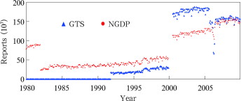
Figure 1 shows the time series of the number of global daily precipitation reports in the original GTS and NGDP datasets. There were less stations reporting daily precipitation before 2000, especially none before 1992. After the upgrade of the GTS receiving system in 2000, the number of daily precipitation records in the original GTS dataset increased significantly. In the QC process, missing daily precipitation records were complemented by hourly precipitation reports. As a result, the number of daily precipitation records increased significantly after the QC. Further analysis shows that, except for the internal consistency check which complemented daily precipitation dataset using hourly precipitation, all other QC checks led to some decrease in the number of daily precipitation records. The results indicate that approximately 80% of the data passed all QC checks. The percentage is as high as 18% which failed the consecutive duplication check. About 2% were removed by other QC checks.

Figure 1. Time series of daily precipitation reports in the original GTS dataset and the NGDP dataset after QC

The fact that erroneous data were detected in every QC step shows that QC for global gauge-based daily precipitation is a complex process. A comprehensive approach taking into account of all kinds of errors can improve the overall efficiency of the QC process.

4.2. Intensity frequency

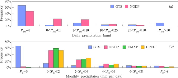
Examination of the frequency of precipitation intensity provides us with a qualitative sense of how well the relative intensity of precipitation events are reproduced in the post-QC precipitation data. Figure 2a shows the frequency distribution of daily precipitation at different intensity levels for pre- and post-QC datasets (no rain, P_24h = 0 mm; dribble, 0 mm < P_24h ≤ 1 mm; light, 1 mm<P_24h ≤ 10 mm; moderate, 10 mm<P_24h ≤ 25 mm; heavy, 25 mm<P_24h ≤ 50 mm; storm, P_24h > 50 mm). In the original GTS dataset, the frequencies for no rain and storm are obviously too high. The QC process removed the outliers. As a result, the frequencies of no rain and storm are significantly lower in the NGDP dataset. After QC checks, the decreasing trend in frequency distribution with increasing precipitation intensities was more prevalent and reasonable.

Figure 2. Frequency distributions of different intensities (mm per day) (a) for daily precipitation in the original GTS dataset and NGDP dataset; and (b) for monthly precipitation amount in the original GTS dataset, the NGDP dataset, the CMAP dataset and the GPCP dataset

Figure 2 b gives the frequency distribution of monthly mean precipitation. There are significant differences between the original GTS data and the CMAP and GPCP products. The frequencies of no rain events and 0–4 mm per day events are 65.5% and 2.7%, respectively, which are significantly different from those of the CMAP and GPCP. After QC checks, the probability density of NGDP monthly precipitation intensity is almost the same as that of CMAP and GPCP. This result shows that the frequency distribution of monthly precipitation intensity is reasonable in the NGDP dataset.

4.3. Scatter Graph analysis

Figure 3 presents scatter plots of the annual precipitation of the original GTS, NGDP, and GPCP datasets comparing to that of CMAP dataset. It is clear that the original GTS annual precipitation is significantly overestimated comparing to the CMAP, with most of scatter points locating on the left part of the diagonal (Fig. 3a ). The annual precipitation of the NGDP dataset shows a better fit to that of the CMAP than of the original GTS dataset, with a more evenly scatter distribution around the diagonal (Fig. 3b ). Moreover, this fitting relationship is similar to that of the GPCP versus CMAP (Fig. 3c ). These results show that QC checks significantly improved annual precipitation in the GTS dataset.

Figure 3. Scatter plots of annual precipitation in the CMAP data versus those in (a) the original GTS dataset, (b) NGDP dataset, and (c) GPCP dataset

4.4. Spatial correlation analysis

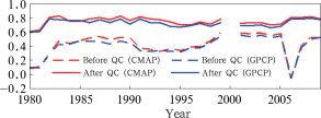
Figure 4 provides the global average spatial correlation coefficients between gauge-based monthly precipitation and the corresponding CMAP and GPCP monthly precipitation^① . Because there were no daily precipitation records in the original GTS dataset before 1992, daily precipitation resulted from the internal consistency check were used to compare with the NGDP data.

Figure 4. The time series of the global average spatial correlation coefficients of the global gauge precipitation datasets before QC and after QC with the CMAP and GPCP datasets

On average (the 30-year average from 1981 to 2009), the global mean spatial correlation coefficients between the original GTS and the CMAP and GPCP were lower than 0.4 with much greater interannual variability. After QC checks, the spatial correlation coefficients increased steadily over 0.6 and the 30-year average coefficients reached 0.7 with smooth interannual variability in both cases (CMAP and GPCP). The results indicate that the global spatial distribution patterns of the GTS precipitation have been improved significantly after QC checks, suggesting good spatial pattern consistency with the CMAP and GPCP precipitation products.

4.5. Temporal correlation coefficient and root mean square error (RMSE) analysis

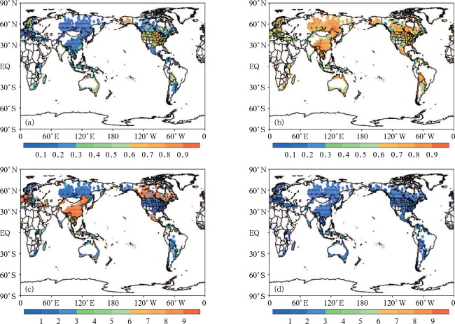
Figure 5 presents the spatial distribution pattern of temporal correlation and RMSE between monthly precipitation of the gauge-based data and the CMAP data. In most areas with dense gauge networks (e.g., Asia, North America, and Europe), the correlation between the original GTS precipitation and the CMAP is lower than 0.3, and the RMSE are higher than 9 mm per day. After QC checks, both the correlation and RMSE for the NGDP data are improved significantly. In those same areas, the area-mean correlation coefficients reach 0.7, while the RMSE’s are reduced to lower than 2 mm per day.

Figure 5. Spatial distributions of the correlation coefficients and RMSE (mm per day) between monthly precipitation of global gauge data and CMAP data, (a) correlation coefficients of the original GTS data, (b) correlation coefficients of the NGDP data, (c) RMSE of the original GTS data, and (d) RMSE of the NGDP data

Table 1 shows the global mean temporal correlation coefficients and RMSE of the original GTS data and NGDP data comparing with CMAP and GPCP. For the original GTS data, the annual mean correlation coefficient is only 0.24 with CMAP and GPCP data, while the RMSE is as high as 12 mm per day. Both the correlation coefficient and RMSE have obvious seasonal fluctuations, with the maximum errors in spring. After QC checks, the annual mean correlation coefficient is improved significantly (0.69). The RMSE of the NGDP dataset is reduced by more than 90% of the original GTS data, with an annual average of only 1 mm per day. The seasonal fluctuations of RMSE are also eliminated substantially. These results show that the NGDP precipitation dataset has a very good reliability.

Table 1. Global mean correlation coefficients and RMSE of precipitation in the original GTS dataset and NGDP comparing with CMAP and GPCP in spring (MAM), summer (JJA), autumn (SON), winter (DJF), and the annual mean (ANN)

		CMAP					GPCP
		MAM	JJA	SON	DJF	ANN	MAM	JJA	SON	DJF	ANN
	GTS	0.25	0.21	0.46	0.44	0.24	0.25	0.21	0.45	0.44	0.24
correlation coefficient	NGDP	0.64	0.54	0.65	0.57	0.70	0.64	0.53	0.64	0.57	0.69
RMSE (mm per day)	GTS	31	12	2	2	12	31	12	2	2	12
	NGDP	1	2	1	1	1	1	2	1	1	1

4.6. Interannual variability

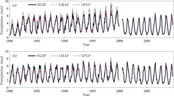
Figure 6 illustrates the time series of monthly precipitation from the NGDP dataset and CMAP dataset and GPCP dataset over Asia. The series of CMAP and GPCP data are obtained by calculating regional average of derived station data which are interpolated from the original grid data. Figure 6a shows that NGDP data lie between the CMAP and GPCP data during most of the time except the 1990s, when the peak values of NGDP data are lower than CMAP and GPCP data due to the lack of records. There is also a noticeable “jump” around 2000 for all three datasets. The significant change in number of records in the GTS dataset in 2000 (Fig. 1 ) led to a sudden change in the number of stations with precipitation records and thus an obvious jump in the regional averages.

Figure 6. Time series of regional mean monthly precipitation in Asia, (a) data from all rain-gauges, and (b) data from rain-gauges with more than 22 years daily records

In order to avoid the impact of significant change in number of stations on regional mean precipitation, only those stations with more than 22 years daily records were used in the construction of regional mean time series (Fig. 6b ). The jump around 2000 as shown in Figure 6a disappeared. Further more, the time series of NGDP dataset is more consistent with those of CMAP and GPCP datasets than in Figure 6a . These results indicate that after applying QC, the interannual variability of the gauge-based precipitation dataset is more in line with that of the CMAP and GPCP products when the contributing stations have sufficiently long records.

4.7. Seasonal cycle

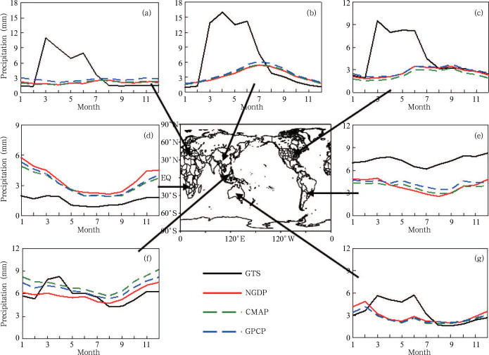
Figure 7 provides the seasonal cycle of monthly precipitation averaged over 1980–2009 in different land areas over the world. In Europe, Asia, North America, and Australia, due to incorrect record units and other decoding errors from March to July 2006, the precipitations from the original GTS dataset are much larger than those from the CMAP and GPCP datasets. In South America, southern Africa, and Equatorial Islands, the pattern and intensities of seasonal variability from the original GTS data also show obvious difference with those from the CMAP and GPCP data. After QC checks, the seasonal cycles for all land regions are improved significantly. The serious biases of seasonal cycle in Europe, Asia, North America, and Australia have been eliminated successfully. Except for Equatorial Islands, the intensity and pattern of seasonal variations in NGDP dataset are in good agreement with those of the CMAP and GPCP datasets. Due to the limit of fewer GTS stations over Equatorial Islands, the improvement from the QC process is weaker than other regions. However, compared to the original GTS data, the seasonal cycle of the NGDP dataset is much more close to the CMAP and GPCP datasets. Overall, the precipitation in the NGDP dataset can accurately represent the seasonal variations of monthly precipitation in most global land areas.

Figure 7. Seasonal cycles of the original GTS data, the NGDP data, the CMAP data, and the GPCP data in different regions (a) Europe, (b) Asia, (c) North America, (d) southern Africa, (e) South America, (f) Equatorial islands, (g) Australia

5. Conclusions and discussion

(1) QC procedures with five steps, including duplication station check, internal consistency check, extreme value check, temporal consistency check, and spatial consistency check, have been performed on a gauge-based global daily precipitation from “the global surface synoptic dataset” for the period 1980–2009. The NGDP dataset has been constructed after the QC procedures.

(2) The frequency distribution of monthly precipitation and scatter graphs of annual precipitation in the NGDP dataset are consistent with the CMAP and GPCP datasets. The 30-year average global mean spatial correlation coefficients of the NGDP with both CMAP and GPCP data increased to 0.7. The global spatial distribution patterns of the NGDP dataset have been improved significantly after QC checks.

(3) The temporal correlation coefficients of NGDP data with the CMAP and GPCP products can reach 0.69 and 0.70, respectively, which is a significant improvement compared to that of the original GTS dataset. Meanwhile, the global mean RMSE’s have been reduced from 12 to 1 mm per day by QC checks.

(4) The interannual and seasonal variabilities of the NGDP dataset are consistent with that of CMAP and GPCP datasets.

The ultimate goal of QC checks is to ensure accuracy and reliability of the data. This study improved the overall quality of the original GTS daily precipitation dataset, and provides a reliable global gauge-based precipitation dataset for operational climate monitoring and climate change researches in China. However, since most of the available GTS precipitation data are from land and island stations, both the coverage and the quality over the oceans are far from our need. Therefore, it is necessary to assimilate gauge-based precipitation data such as the NGDP dataset with satellite-based precipitation data. In the future, we will attempt to combine this NGDP dataset with a variety of satellite precipitation products to get a quasi-real-time reanalysis precipitation dataset.

Acknowledgements

The authors thank the National Meteorological Information Center of China Meteorological Administration for the original GTS dataset. This research was supported by the National Natural Science Foundation (No. 40905046, No. 41175066), the National High Technology Research and Development Program (No.2009AA1220005, No.2009BAC51B03) and the National Basic Research Program (No. 2010CB951902) of China.

References

1. Adler et al., 2003 R.F. Adler, G.J. Huffman, A. Chang, et al.; The version 2 Global Precipitation Climatology Project (GPCP) monthly precipitation analysis (1979–present); Journal of Hydrometeorology, 4 (6) (2003), pp. 1147–1167
2. Eischeid et al., 1995 J.K. Eischeid, C.B. Baker, T. Karl, et al.; The quality control of long-term climatological data using objective data analysis; Journal of Applied Meteorology and Climatology, 34 (12) (1995), pp. 2787–2795
3. Graybeal et al., 2004 D.Y. Graybeal, A.T. DeGaetano, K.L. Eggleston; Complex quality assurance of historical hourly surface airways meteorological data; Journal of Atmospheric and Oceanic Technology, 21 (8) (2004), pp. 1156–1169
4. Harmel et al., 2002 R.D. Harmel, C.W. Richardson, C.L. Hanson, et al.; Evaluating the adequacy of simulating maximum and minimum daily air temperature with the normal distribution; Journal of Applied Meteorology and Climatology, 41 (7) (2002), pp. 744–753
5. Hubbard et al., 2005 K.G. Hubbard, S. Goddard, W.D. Sorensen, et al.; Performance of quality assurance procedures for an applied climate information system; Journal of Atmospheric and Oceanic Technology, 22 (1) (2005), pp. 105–112
6. Huffman et al., 1997 G.J. Huffman, R.F. Adler, P. Arkin, et al.; The Global Precipitation Climatology Project (GPCP) combined precipitation dataset; Bulletin of the American Meteorological Society, 78 (1) (1997), pp. 5–20
7. Kunkel et al., 2005 K.E. Kunkel, D.R. Easterling, K. Redmond, et al.; Quality control of pre-1948 cooperative observer network data; Journal of Atmospheric and Oceanic Technology, 22 (11) (2005), pp. 1691–1705
8. Kunkel et al., 1998 K.E. Kunkel, A. Karen, C. Glen, et al.; An expanded digital daily database for climatic resources applications in the Midwestern United States; Bulletin of the American Meteorological Society, 79 (7) (1998), pp. 1357–1366
9. Lanzante, 1996 J.R. Lanzante; Resistant, robust and nonparametric techniques for analysis of climate data: Theory and examples, including applications to historical radiosonde station data; International Journal of Climatology, 16 (1996), pp. 1197–1226
10. Liljegren et al., 2009 J.C. Liljegren, T. Stephen, R. Kevin, et al.; Quality control of meteorological data for the chemical stockpile emergency preparedness program; Journal of Atmospheric and Oceanic Technology, 26 (8) (2009), pp. 1510–1526
11. Liu et al., 2006 X.-N. Liu, X.-H. Ju, S.-H. Fan; A research on the applicability of spatial regression test in meteorological datasets; Journal of Applied Meteorological Science (in Chinese, 17 (1) (2006), pp. 37–43
12. Ren and Zhai, 1998 F.-M. Ren, P.-M. Zhai; Study on changes of China’s extreme temperatures during 1951–1990; Scientia Atmospherica Sinica (in Chinese), 22 (2) (1998), pp. 217–227
13. Tao et al., 2009 S.-W. Tao, Q.-Q. Zhong, Z.-F. Xu, et al.; Quality control schemes and its application to automatic surface weather observation system; Plateau Meteorology (in Chinese), 28 (5) (2009), pp. 1202–1209
14. Wang et al., 2001 B. Wang, R.-G. Wu, K.M. Lau; Interannual variability of the Asian summer monsoon: Contrasts between the Indian and the Western North Pacific-East Asian Monsoons; J. Climate, 14 (20) (2001), pp. 4073–4090
15. Wang et al., 2006 X.-L. Wang, F.-M. Ren, W. Li, et al.; An operational global station climatological daily data set for climate; Meteorological Monthly (in Chinese), 32 (3) (2006), pp. 39–43
16. Wolter, 1997 K. Wolter; Trimming problems and remedies in COADS; J. Climate, 10 (8) (1997), pp. 1980–1997
17. Xie and Arkin, 1997 P.-P. Xie, P.-A. Arkin; Global precipitation: A 17-year monthly analysis based on gauge observations; satellite estimates, and numerical model outputs. Bulletin of the American Meteorological Society, 78 (11) (1997), pp. 2539–2558
18. Zhang et al., 2004 Q. Zhang, F.-H. Guo, S. Xu; Quality control and analysis of data set characteristic for global surface synoptic reports; Journal of Applied Meteorological Science (in Chinese), 15 (2004), pp. 121–127

Notes

①. Firstly, CMAP and GPCP grid data are interpolated into global stations using bilinear interpolation method. Then, the spatial correlation coefficients are calculated between interpolated CMAP and GPCP data and GTS gauge-based data