Experimental characterization and two-dimensional hydraulic-hydrologic modelling of the infiltration process through permeable pavements

Abstract

Permeable pavements are a common solution for wearing course layers in roads and urban areas. They are composed by highly porous materials with permeability several orders of magnitude above of the natural terrain. This work presents, on one hand, the experimental characterisation of the hydraulic behaviour of a permeable asphalt concrete wearing course layer and, on the other hand, the development and validation of a two-dimensional coupled hydraulic-hydrological distributed numerical model to reproduce the effect of the infiltration in the rainfall-runoff transformation and in the overland flow propagation processes. Experiments show linear and potential trends for permeability-hydraulic head relations when considering constant and variable hydraulic heads, respectively, reaching permeability up to 0.04 m/s for 1 m of hydraulic head. Experiments are reproduced numerically by incorporating new infiltration formulas, which consider the infiltration rate as a function of the hydraulic head, and a specific numerical scheme for properly dealing the mass conservation when negative values of the water depth may occur numerically due to high infiltration rates. This two-dimensional coupled hydraulic-hydrological distributed numerical model is a validated tool for simulating the effect of permeable pavements not only in the rainfall-runoff process, but also for the overland flow propagation.

Keywords: Permeable pavement, SUDS, numerical modelling, 2D-SWE, validation

1. Introduction

The complexity of a fluid flow in porous media is, in general, directly related to the heterogeneity of the channels network created by the connexion between pores [1–4]. Its analysis, from a theoretical point of view, requires simplifications leading to a solution far from the reality of the physical phenomenon to assess [5]. Therefore, the problem has traditionally been addressed through laboratory tests.

Darcy’s Law [6], developed in an eminently practical way [7], makes it possible to relate the filtration velocity ( ${\textstyle v}$ ) and the hydraulic gradient ( ${\textstyle i}$ ) by means of a linear proportionality coefficient, known as permeability ( ${\textstyle k}$ ). This law is widely accepted for laminar flow in a porous media, i.e. for small values of the hydraulic gradient and Reynolds numbers between 1 and 10, although some authors extend it up to 75 [3,8]. However, for high porosity media, such as permeable pavement, inertial forces are not negligible. Therefore, a linear approximation, as the one proposed by Darcy, would not be entirely valid [9].

According to Chauveteau and Thirriot [4], four different regimes depending on the Reynolds number exist: 1) laminar with linear pressure drop; 2) laminar with non-linear pressure drop; 3) mixed (laminar in some pores and turbulent in others); and 4) turbulent regime. The aforementioned work shows how a Reynolds number of 180 is necessary to achieve a fully developed turbulent regime in the pores (4^th stage). Due to the general heterogeneity of the porous material, especially in permeable pavements, it is difficult to determine a limiting Reynolds number [4]. A detailed study of this parameter would also entail characterising the medium itself [10].

For highly porous media, whose hydraulic gradient is high, various approaches have also been proposed of an experimental nature, such as, for example, second and third order polynomial types without an independent term proposed by Forchheimer, potential types by Wikins and Escade [3], exponential approach [11], or like those proposed by Seelhiem and Schilchter for turbulent and laminar regimes that are a function of the diameter of the grain [12].

In the present day, there are several methods to measure infiltration rates of permeable pavements [13]. These measurements are usually performed in situ over a particular section of the pavement and are based on a certain type of modified single or double ring infiltrometer test [14]. Under these conditions, the water is supplied to the test using either constant or variable hydraulic head.

It is essential to be aware of the fluid behaviour through porous media, especially in hydrology, to accurately characterise physical phenomena such as the infiltration process [15]. This may lead to a good characterisation of the rainfall-runoff transformation process and, thus, to a good representation of the overland flow, which is an important parameter in flood risk analysis.

In this sense, several hydrological modelling tools are available for practitioners [16–30] that include the most common infiltration formulas [15]. However, those formulas were proposed for low infiltration velocities, mainly related to porous media with low permeability such as those found in the nature. Since the implementation of Sustainable Urban Drainage Systems (SUDS) are a solution used increasingly in urban areas, the characterisation of highly porous media is necessary to assess its effectiveness from a hydrological and hydraulic perspective.

Against this background, this work aims at developing and integrating the infiltration processes specific of permeable pavements in a two-dimensional numerical tool. Hence, the hydraulic behaviour of a permeable asphalt wearing course layer was analysed in the laboratory. The characterisation of the infiltration capacity of this pavement allowed, under different hydraulic conditions, to calibrate and validate a coupled hydraulic-hydrological distributed numerical model based on the solution of the two-dimensional Saint-Venant Equations. A few applications and considerations are also discussed when this type of numerical models are employed for urban flood risk analysis.

2. Materials and methods

2.1 Experimental design and tests

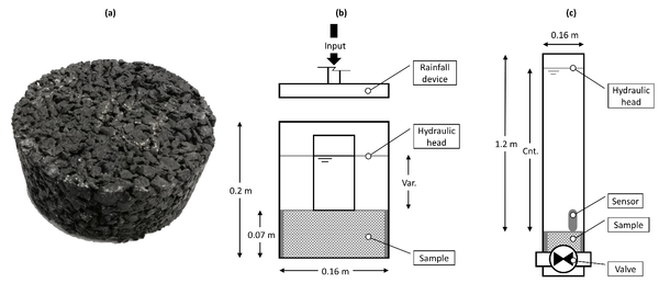
The sample of permeable pavement tested is a cylindrical beam of asphalt with a height of 0.07 m and a diameter of 0.15 m that represents a wearing course layer of an asphalt concrete. It is characterised by BM3-C asphalt binder with PMB 50/70 designation-type, granitic arid with a mean diameter of 0.011 m and a porosity of 23% (Figure 1a).

Since the flow through a permeable pavement is a function not only of the percentage of voids of the material, but also of the configuration of the material’s matrix, two experiments have been performed to evaluate the vertical permeability of the sample. Experiment 1 (Exp. #1) simulates the permeability under different constant hydraulic heads, whereas experiment 2 (Exp. #2) reproduces the permeability considering variable hydraulic head conditions.

Exp. #1 consists on pouring rainfall with constant intensity over the sample keeping a constant hydraulic head on the surface of the sample. The facility was a circular PVC pipe of 0.2 m of length and a diameter of 0.16 m (Figure 1b). The sample was placed at the bottom the pipe, while a rainfall simulator device supplied water from the upper part under conditions close to the reality. A small window of acrylic was created in the pipe to observe the water behaviour over the sample and to control the water depth visually. Permeability and water depth measurements were conducted by collecting the water volume during a fixed time and with a limnimeter, respectively. Twelve hydraulic heads were examined, from 0 m (“dry” conditions on the sample) to 0.11 m of water depth with intervals of 0.01 m each.

Exp. #2 was a facility that provided variable hydraulic head conditions by a valve opening. A fixed water volume, equivalent to 0.97 m of water depth, was stored in a PVC pipe that was 1.2 m long and 0.16 m of diameter with a valve at the bottom of the device (Figure 1c). The sample was placed over the valve, which instantaneously released the stored water through the sample once it was opened. The water depth was measured each second by means of an absolute pressure sensor HOBO Water Level Logger (0 to 9 m), with a precision of ±1.4 mm, which was placed vertically inside the pipe.

Figure 1. Experimental design. (a) Photography of the permeable pavement (sample). (b) Sketch of the Exp. #1 facility (frontal view).
(c) Sketch of the Exp. #2 facility (frontal view)

All experimental tests were repeated in order to to filtrate measurement errors and to obtain consistent data. Subsequently, mean of the recorded data was taken to obtain the final outcome.

2.2 Numerical model and configuration

Experimental tests were reproduced numerically with the free surface flow modelling tool named Iber [31–33]. Iber is a hydraulic model that provides solutions to the two-dimensional Shallow Water Equations, or 2D-SWE, over a mesh of structured and/or unstructured elements. It uses a conservative scheme based on the Finite Volumes Method (FVM), specifically Roe’s high-resolution scheme [34] which consists of the Godunov method together with the Roe Approximate Riemann Solver [35].

Among the calculation modules incorporated by Iber [36–41], a module for the evaluation of hydrological processes also exists, which is fully integrated with the hydrodynamic module [42–46]. Therefore, it is a coupled hydrological-hydraulic distributed model based on the solution of the 2D-SWE, which solves the equations of conservation of mass and momentum described in Equation (1)

{\begin{matrix}\displaystyle {\frac {\delta h}{\delta t}}+\displaystyle {\frac {\delta h{U}_{x}}{\delta x}}+\displaystyle {\frac {\delta h{U}_{y}}{\delta y}}=R-f\\\displaystyle {\frac {\delta h{U}_{x}}{\delta t}}+\displaystyle {\frac {\delta h{U}_{x}^{2}}{\delta x}}+\displaystyle {\frac {\delta h{U}_{x}{U}_{y}}{\delta y}}=gh\left({S}_{o,x}-{S}_{f,x}\right)\\\displaystyle {\frac {\delta h{U}_{y}}{\delta t}}+\displaystyle {\frac {\delta h{U}_{x}{U}_{y}}{\delta x}}+\displaystyle {\frac {\delta h{U}_{y}^{2}}{\delta y}}=gh\left({S}_{o,y}-{S}_{f,y}\right)\end{matrix}}

(1)

where ${\textstyle h}$ is the water depth, ${\textstyle {U}_{x}}$ and ${\textstyle {U}_{y}}$ are the ${\textstyle X}$ and ${\textstyle Y}$ component of the velocity, ${\textstyle g}$ is the gravitational acceleration, ${\textstyle {S}_{o,x}}$ and ${\textstyle {S}_{o,y}}$ are the ${\textstyle X}$ and ${\textstyle Y}$ component of the slope of bottom, ${\textstyle {S}_{f,x}}$ and ${\textstyle {S}_{f,y}}$ are the X and Y component of bottom friction.

The main difference with the classical 2D-SWE for hydrodynamics is the appearance of the source terms ${\textstyle R}$ and ${\textstyle f}$ in the mass conservation equation, which represent the intensity of precipitation and the hydrological losses, respectively. The term ${\textstyle f}$ include processes such as infiltration, evapotranspiration, interception and surface retention. Subsequently, these processes may or may not be considered in dependent sub-processes, including subsurface flow, accumulation and transport through the aquifer, exfiltration, etc.

The 2D-SWE (Equation (1)) are solved in each element of the calculation mesh integrating it in the space using the Gauss theorem and in time through an explicit Euler scheme. The ${\textstyle R}$ and ${\textstyle f}$ terms, as well as the free surface gradient and the bed friction stress terms, follow a centred discretisation, while the mass flow and momentum are approximated with an upwind scheme. In this way, the flow that leaves an element is the same as that enters the adjacent element through the adjoining side; hence, the conservation of mass is guaranteed throughout all the calculation mesh. A detailed description of the numerical scheme used in Iber can be found in Cea and Bladé [42].

The permeability in highly porous media, such as permeable pavements, supposes infiltration rates several orders of magnitude above those usual in hydrology. This can lead to negative values of the water depth during the resolution of the 2D-SWE, from few millimetres to several centimetres of the water depth. Therefore, the mass conservation equation is solved in two steps. In the first step, an intermediate state of the water depth ( ${\textstyle {h}^{\ast }}$ ) is obtained considering the intensity of rain and the mass flow between the adjacent elements (Equation (2))

(2)

where ${\textstyle {h}_{i}^{n}}$ is the water depth of element ${\textstyle \,i}$ evaluated at time ${\textstyle n}$ , ${\textstyle {Q}_{ij}^{n}}$ is the numerical approximation of the mass flow between adjacent elements at time ${\textstyle n}$ , ${\textstyle {A}_{i}}$ is the area of element ${\textstyle i}$ , ${\textstyle \Delta t}$ is the computational time step which is limited by the Courant–Friedrichs–Lewy condition [47] and ${\textstyle {R}_{i}^{n}}$ is the intensity of precipitation in the element ${\textstyle i}$ at instant ${\textstyle n}$ .

In the second step, ${\textstyle {h}^{\ast }}$ is reduced by any of the hydrological losses ( ${\textstyle f}$ ) described previously to obtain the depth at the next time step (Equation (3))

(3)

where ${\textstyle {h}_{i}^{n+1}}$ is the water depth of the element ${\textstyle i}$ evaluated at time ${\textstyle n+}$ $1$ and ${\textstyle {f}_{i}^{n}}$ is the loss of water volume in the element ${\textstyle i}$ at time ${\textstyle n}$ . To ensure positive values of the water depth at time ${\textstyle n+}$ $1$ , losses are limited considering the volume of water present in the element at time ${\textstyle n}$ . Thus:

(4)

where ${\textstyle {f}_{i}^{pot}}$ t is the potential capacity to produce losses in the element ${\textstyle i}$ .

For permeable pavements, and specifically those that allow complete water infiltration into deeper layers, the parameter ${\textstyle {f}_{}^{pot}}$ can be evaluated according to infiltration formulas commonly used in the field of hydrology [15]. Iber incorporates the most common models: the linear model with initial losses, the Green-Ampt model [48], the Soil Conservation System (SCS) model based on the Curve Number method [49–51] and the Horton model [52,53]. However, these formulations were developed for infiltration processes in soils whose characteristics differ from those of a highly porous medium, such as permeable pavements.

Thereby, the code of Iber has been adapted to accommodate a greater number of formulations. For the case study, which can be related to SUDS, it is proposed to use first and second order polynomial infiltration formulations, logarithmic in base 10, potential and direct relationships between hydraulic head and infiltration. All of the formulations are detailed in Table 1.

Table 1. Formulations implemented in Iber and expressed as potential infiltration capacity (

)

Model	# parameters	Formulation	Description
Linear + initial losses	2	${\begin{matrix}{f}_{}^{pot}=f&si\,h\,o\,R>\,{I}_{a}\\{f}_{}^{pot}={\frac {{I}_{a}}{t}}&si\,h\,o\,R\leq \,{I}_{a}\end{matrix}}$	${\textstyle {I}_{a}}$ is the initial losses that, until they are overcome by precipitation or the amount of water in the element, there are no linear losses ( ${\textstyle f}$ ).
Green-Ampt [48]	3-6	${f}_{}^{pot}={k}_{s}\left(1+{\frac {\left(h+\psi \right)}{b}}\right)$ where, ${\begin{matrix}b={b}_{0}+{\frac {F}{\phi }}&F=\displaystyle \int _{0}^{t}f\,dt\end{matrix}}$ ${\begin{matrix}{\frac {b}{{d}_{s}}}={\frac {\theta }{\phi }}&{b}_{0}={\theta }_{0}{\frac {{d}_{s}}{\phi }}\end{matrix}}$	${\textstyle {k}_{s}}$ is the saturated permeability of the soil in the vertical direction, ${\textstyle h}$ is the water depth on the ground, ${\textstyle \psi }$ is the suction in the unsaturated soil layer; ${\textstyle b}$ is the thickness of the saturated soil layer, ${\textstyle {b}_{0}}$ is the initial thickness of the saturated soil layer and ${\textstyle \phi }$ is the porosity of the soil. In Iber the thickness of the saturated soil layer ( ${\textstyle b}$ ) is related to the vertically averaged moisture content in the soil layer ( ${\textstyle \theta }$ ), where ${\textstyle {d}_{s}}$ is the total thickness of the soil layer and ${\textstyle \phi }$ its porosity, and ${\textstyle {\theta }_{0}}$ is the initial soil moisture.
SCS [49–51]	2	${f}_{}^{pot}={\frac {{F}_{(t+\Delta t)}-{F}_{\left(t\right)}}{\Delta t}}$ where, $F=P-{P}_{n}$ ${\begin{matrix}{P}_{n}={\frac {{\left(P-\alpha \,S\right)}^{2}}{P+\left(1-\alpha \right)\,S}}&P>\alpha \,S\end{matrix}}$ $S={\frac {25400}{CN}}-254$	The infiltration accumulated in two consecutive time steps ( ${\textstyle {F}_{\left(t\right)}}$ and ${\textstyle {F}_{(t+\Delta t)}}$ ) allows to calculate ${\textstyle {f}_{}^{pot}}$ . ${\textstyle F}$ depends on the difference between gross precipitation ${\textstyle P}$ and net ${\textstyle {P}_{n}}$ . When ${\textstyle P}$ is greater than the initial losses, evaluated as ${\textstyle \alpha \,S}$ (normally ${\textstyle \alpha }$ = 0.2), ${\textstyle {P}_{n}}$ will be calculated following the formulation proposed by the SCS that depends on the curve number ( ${\textstyle CN}$ ), a parameter related to the type of land, land uses and land slopes.
Horton [52,53]	3	$\Delta {F}_{pot}={f}_{r}\,\Delta t+{\frac {\left({f}_{0}-{f}_{r}\right)}{k}}\left(1-\right.$ $\left.{e}^{-k\,\Delta t}\right)$ ${\textstyle {f}_{o}={f}_{r}+\left({f}_{0}-{f}_{r}\right)\,{e}^{-k\,\Delta t}}$ if ${\textstyle \Delta {F}_{pot}\leq h}$ ${\textstyle {f}_{o}={f}_{r}+\left({f}_{0}-{f}_{r}\right)\,{e}^{-k\,{\frac {h}{f}}}}$ if ${\textstyle \Delta {F}_{pot}>h}$	At each time step, ${\textstyle {f}_{pot}}$ is calculated as the integral ${\textstyle t}$ and ${\textstyle t+}$ $\Delta t$ , and the value of ${\textstyle {f}_{0}}$ is updated. That is, with this discretization, if there is no rain or no water in the element, no water infiltrates and the potential infiltration rate stops decreasing since the soil moisture is not increasing.
Polynomial 1^st order	2	${f}_{}^{pot}=\alpha h+\beta$	As long as there is enough water in the element ( ${\textstyle h>\beta \Delta t}$ ), ${\textstyle {f}_{pot}}$ will follow a linear infiltration law.
Polynomial 2^nd order	3	${f}_{}^{pot}=\alpha {h}^{2}+\beta h+\gamma$	As long as there is enough water in the element ( ${\textstyle h>\gamma \Delta t}$ ), ${\textstyle {f}_{pot}}$ will follow a quadratic infiltration law.
Logarithmic (base 10)	2	${f}_{}^{pot}=\alpha log\left(h\right)+\beta$	As long as there is enough water in the element ( ${\textstyle h>\beta \Delta t}$ ), ${\textstyle {f}_{pot}}$ will follow a logarithmic infiltration law.
Potential	2	${f}_{}^{pot}=\alpha {h}^{\beta }$	As long as there is enough water in the element, ${\textstyle {f}_{pot}}$ will follow a potential infiltration law.
Table ${\textstyle h-f}$	variable	${f}_{}^{pot}=f\left(h\right)$	For each value of ${\textstyle h}$ , a value of ${\textstyle f}$ is obtained as long as there is sufficient amount of water. Intermediate values are linearly interpolated.

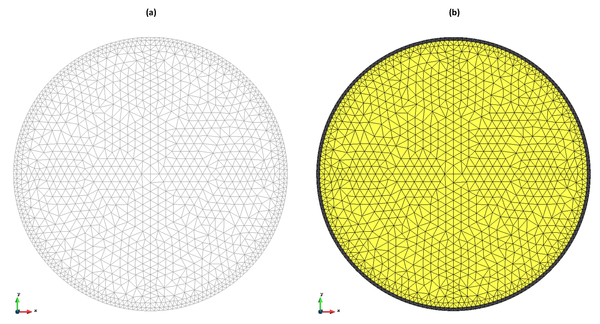
The model setup was identical for all the tests performed. The geometry of each experiments was discretised using an unstructured mesh of triangular elements generated in GiD [54–56], whose minimum side size was 0.0018 m and the maximum side was 0.0086 m. This configuration imposes smaller elements at the contour (Figure 2), since the sample, centred in the device, has an area slightly lower (0.0176 m²) than the section of the tube where the pavement sample was installed (0.0185 m²). The domain was discretised with a ratio equivalent to 128,325 elements per square meter, a value several orders of magnitude above the one that is commonly used in flood studies [57]. The first order Roe scheme was used, and the friction in the walls was not considered due to the reduced roughness of the tube material (PVC).

Figure 2. Numerical discretisation of the geometry of the tests. (a) calculation mesh. (b) Location of the elements that represent the permeable pavement sample (yellow) and the non-permeable zone (dark grey)

3 Results and discussion

3.1 Permeability at constant hydraulic head

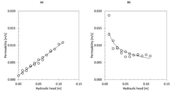
In Exp. #1, when the desired hydraulic head was reached, the volume of the water flowed through the sample was collected and then measured for a time interval of 30 s. Thus, the infiltration rate associated to a particular hydraulic head was obtained. Figure 3a shows the results of permeability and how the results follow a linear trend. By contrast, when applying Darcy’s law to the previous data, a potential trend is obtained providing infinite permeability when the hydraulic head tends to zero (Figure 3b). This is one of the reasons why this methodology must not be used to characterise the permeability for highly porous media.

Figure 3. Experimental results of the permeability test at constant hydraulic head. (a) Infiltration rate related to a constant hydraulic head. (b) Infiltration rate related to a constant hydraulic head considering Darcy’s law

The experimental permeability data (Figure 3a) were directly transformed into potential infiltration capacity ( ${\textstyle {f}^{pot}}$ ). The best fit of the depth-infiltration relationship performed by least squares was obtained with a straight line, which resulted in the parameters $\alpha$ = 314 248 and $\beta$ = 4287.7 for a 1^st order polynomial infiltration model (Table 1). This infiltration model was imposed on the elements of the calculation mesh that represents the permeable pavement (Figure 2b, yellow colour). The model was forced with the rainfall intensity associated with the value of the water depth observed during the tests, allowing validating the numerical model under steady conditions.

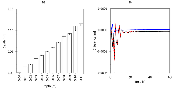
Figure 4a shows the simulated water depth at the centre of the sample when the steady state was reached. The model adequately reproduces the behaviour of the water observed during the tests. The differences shown for the depths of 0.01, 0.03, 0.08 and 0.10 m (Figure 4a, error bars) can be related to the adjustment of the infiltration model made by means of the regression line. If the model is forced with the observed infiltration data using the Table ${\textstyle h-}$ $f$ model (Table 1), the expected water depth is accurately obtained.

Additionally, a sensitivity analysis for the mesh-size was performed for the precipitation value corresponding to a hydraulic head of 0.06 m. The calculation domain was discretised with a finer and coarse meshes, which represents a ratio of 53,190 and of 2,285,297 els./m², respectively. Figure 4b shows, on the one hand, the difference in the evolution of the depth obtained with the coarse and the intermediate meshes with respect to the finest (black and red lines) and, on the other hand, the difference in the depth between the coarse and intermediate meshes (blue line). In general, the differences are minute (< 0.0002 m), stabilising after 20 s of the simulation at lower values. It should be noted that the calculation time for an intermediate and fine mesh is multiplied by a factor of 1.48 and 23.5, respectively, compared to the coarse mesh. Therefore, the mesh with an intermediate ratio (128,325 els./m²) provides adequate results with computation times similar to those of the coarse mesh.

Figure 4. Numerical results of the permeability test at constant hydraulic head. (a) Water depth for the different intensities of precipitation tested. (b) Mesh sensitivity analysis for a water depth of 0.06 m, difference in depth between a coarse and a fine mesh (red dashed line), between a medium and a fine mesh (black line) and between a coarse and a medium mesh (blue line)

Finally, the influence of the numerical scheme on the solution was also analysed. For the test corresponding to 0.06 m of hydraulic head, the second order of Roe and the DHD schemes [42], developed ad hoc for the evaluation of hydrological processes, were tested. In general, the DHD scheme represents a speed-up of x1.3 with respect to the 1^st order scheme, while the 2^nd order scheme increases the computation time by x1.1 with respect to the 1^st order scheme. Although the 2^nd order scheme generally provides more accurate hydraulic results, in this case, its use is not an advantage.

3.2 Permeability at variable hydraulic head

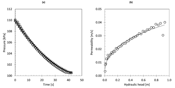
Figure 5a shows the evolution of the water pressure registered in the device of the Exp. #2. Small dispersion was obtained for all tests, confirming the good performance of the device. A potential trend is obtained when averaging the previous data and relating with the hydraulic head (Figure 5b). The reduction of the permeability registered at the second time step (0.902 m) was probably due to the propagation of a wave generated at the opening of the valve.

Figure 5. Experimental results of the permeability test at variable hydraulic head. (a) Absolute pressure observed for all tests. (b) Averaged permeability-hydraulic head relation

Exp. #2 was simulated with a model configuration identical to the one used for a constant hydraulic head (see section 2.2). However, an initial water depth condition equal to 0.97 m was imposed, while there was no water input due to precipitation processes. Based on the experimental results, the infiltration model used in the numerical model was the potential law with ${\textstyle \alpha }$ and ${\textstyle \beta }$ (Table 1) equal to 141,117 and 0.3715, respectively. A mesh size equivalent to 128,325 els./m² was employed as it provides a fair balance between the precision of the results and the computational cost, as demonstrated in section 3.1.

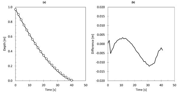
The numerical results conform to the observations during the experiments (Figure 6a). The evolution of the observed water depth follows a second order polynomial trend, characteristic of an emptying process of a pond through a hole. The numerical model, with the infiltration model proposed, follows this same trend with an adjustment of R² = 0.9998.

A detailed comparison between the experimental and numerical results shows that both models differ by less than 0.015 m (in absolute value). These differences are mainly attributable to the oscillation of the free surface due to the wave generated by the opening of the valve. This phenomenon is clearly denoted not only in the reduction of the infiltrated volume observed at the first moments (Figure 5b), but also in the shape of the absolute error between experimental and numerical results (Figure 6b).

Figure 6. Numerical results of the permeability test at variable hydraulic head. (a) Evolution of the water depth for an initial condition of 0.97 m. (b) Absolute error between experimental and numerical results

3.3 Applicability and considerations

The use of permeable pavements as wearing course layer in bitumen packs is common throughout the world [58–63]. However, the infiltration capacity of this type of pavement is conditioned by the layer located immediately below the pavement, which is usually much less permeable, even becoming waterproof according to the technical specifications of the work. Furthermore, the wearing course layer is usually a few centimetres thick, so the flow behaviour in the porous medium is, in general, perpendicular to the surface of the wearing course when it lays over an impervious layer. Although this aspect is not addressed in the present work, its experimental analysis could help to calibrate and validate numerical models that, based or not on the solution of the 2D-SWE, incorporate processes of infiltration and transport through the medium as subsurface flow, along with subsequent exfiltration.

The application of permeable pavements in car parks and roads with light traffic [64,65], where dynamic loads are relatively low and the pavement package under the wearing course layer can be conditioned to continue infiltrating to deeper layers, has shown promising results with infiltration rates of up to 0.008 /s. Similar rates are proved to be in the sample tested herein for relatively low hydraulic heads (less than 0.08 m). It is worth noting that the infiltration capacity increases when the values of the hydraulic head also increases above 0.04 m/s for water depths up to 1 m, as seen in the sample studied. This presumes an infiltration discharge of approximately 40 l/s per square meter.

This type of solutions, applied in urban areas, is known as SUDS (Sustainable Urban Drainage System). SUDS are technical solution intended to increase the permeability of cities, collecting part of the overland flow and/or giving infiltrated water a second use (e.g. irrigation or street cleaning). The main consequence of the reduction of surface runoff is the potential reduction in the hazard and risk of flooding in urban areas [66–68]. They are aligned to the current worldwide trend entitled “sponge cities” [69,70], which is oriented to build cities that are more efficient to manage flood events and water resources stress.

Applying permeable pavements in bicycle lanes could be an alternative to the use of punctual SUDS (such as parking lots or green areas), especially when the urban area is highly consolidated. Bike-lanes are linear elements occupying large amounts of surface and that, in addition, usually cross streets leading, in many cases, to the interception of runoff. Many of them are located on the sides of the road, where the greatest amount of water accumulates. Therefore, its application could potentially reduce the water levels in the streets and, therefore, help in reducing the flood risk.

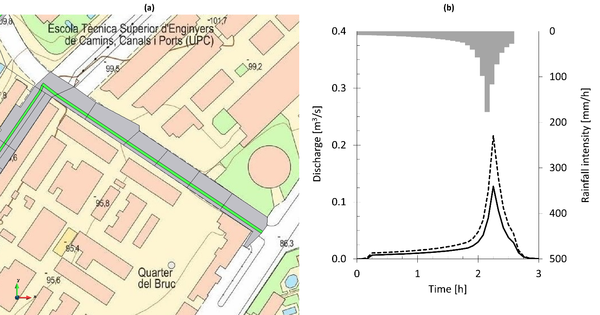
The potential benefits of using permeable pavements are presented through its application in a bike-lane of Barcelona city (Figure 7a). This bike-lane is located on the road and occupies an area of 586.2 m² (Figure 7a, green strip), while the rest of the street occupies 3 811.8 m² (Figure 7a, grey area). The pavement characteristics are based on the linear infiltration model, associated to the experimental data described in section 3.1. A synthetic precipitation event corresponding to a return period of 10 years [71] was used (Figure 7b). The domain was discretized by means of a mesh of triangular elements with a mean side of 2 m, according to the resolution of the digital terrain model. The simulation duration was of 3 h.

Figure 7. Example of application of permeable pavement in a street of Barcelona. (a) Spatial domain of the numerical model, where the green area is the area occupied by the bike-lane that represents the permeable pavement, while the rest of the street is grey (completely waterproof). (b) Outlet hydrograph resulting from surface runoff

Figure 7b shows the outlet hydrograph for two scenarios: without considering permeable pavement (dotted line) and considering permeable pavement in the bike-lane (solid line). The peak flow, considering the permeable pavement, would potentially be reduced by 41%, while the volume of surface runoff would be 38% less. In this case, the effect of the permeable pavement is reduced as the street tends to accumulate the surface runoff on the left side of the street, the opposite side where the bike lane is. Even so, considering that the permeable pavement area only represents 13.3% of the total, the potential benefits of using this type of SUDS would be considerable.

Numerically, for coupled hydrological-hydraulic distributed models based the 2D-SWE, the use of infiltration models associated to very high infiltration capacities may require a specific numerical treatment depending on the scale of analysis [72]. For example, when the behaviour of the overland flow is modified by an inlet element of the sewer system. In such cases, numerical treatments should be addressed at minimizing the unreal acceleration of the flow when large amounts of water infiltrate. An in-depth analysis is therefore necessary in this regard to find a numerical solution that adequately reproduces the physical phenomenon in real conditions.

4. Conclusions

Permeable pavements are a current and recurrent solution as a wearing course layer not only in roads, but also in urban areas as a part of Sustainable Urban Drainage Systems (SUDS). Its application may be oriented to reduce the flood risk through the infiltration of the overland flow, fully or partially. However, their hydraulic and hydrological behaviour must be properly characterised considering that turbulent regime is usually generated when the water flows through this kind of highly porous materials.

The vertical permeability of an asphalt concrete with a common configuration for permeable pavements was experimentally tested under constant and variable hydraulic heads. Permeability up to 0.04 m/s was observed for variable hydraulic head of 1 m, while values greater than 0.001 m/s were obtained under “dry conditions” over the pavement. Experiments demonstrated the necessity of developing ad hoc infiltration formulas, especially for this kind of highly porous media.

Experiments were reproduced numerically with Iber, a coupled hydraulic-hydrological distributed model based on the solution of the 2D-SWE. Hence, the model was adapted by incorporating new infiltration formulas and then validated by reproducing the experiments. For constant hydraulic heads a linear relationship infiltration-depth provided the best adjustment, while a potential law was best fit for a variable hydraulic head less than 1 m. Results allowed validating the numerical tool, showing a good performance with R² > 0.99. The model accurately deal with the mass conservation, even when negative values of the water depth may occur numerically due to high infiltration rates.

Potential benefits of using permeable pavements to reduce the flood risk, both in diagnostic and prognoses scenarios, should be evaluated with correctly validated numerical tools that incorporates, jointly, rainfall-runoff processes and overland flow propagation. We encourage not only to develop and use coupled hydraulic-hydrological distributed numerical models based on the solution of the 2D-SWE, but also to validate it by performing laboratory and field experiments. The development of this kind of numerical tools must be oriented to include sub-processes such as the subsurface flow, the accumulation and transport through the aquifer, the exfiltration, etc., and, when is possible, to connect to the sewer network. All of this should be done with the ultimate aim of providing more accurate tools for assessing and manage flood risk and water resources in urban areas.

Acknowledgements

The present work has been carried out within the framework of the project “Avaluació de SUDS-lineals per reduir el risc d’inundació amb horitzons de Canvi Climàtic” (20S06841-001), co-financed by the Subvecions pel Clima program of the Barcelona City Council. The authors would also like to thank the technical support of M. Griñón and X. Martínez, as well as their experience in the contextualisation and execution of laboratory experiments.

References

[1] San Mauro J., Toledo M., Salazar F., Caballero F.J. A methodology for the design of dam spillways with wedge shaped blocks based on numerical modeling. Rev. Int. Métodos Numéricos Para Cálculo y Diseño En Ing., 35(1), 3, 2019. https://doi.org/10.23967/j.rimni.2018.11.001.

[2] Sánchez Fuster I., López Chacón L., Capilla Romá J.E. Investigación del flujo y transporte mediante experimentación a escala intermedia. Ing. Del Agua, 15(3):147-162, 2008. https://doi.org/10.4995/ia.2008.2932.

[3] Dudgeon C.R. Wall effects in permeameters. J. Hydraul. Div., 93:137–148, 1967. https://doi.org/10.1061/JYCEAJ.0001673.

[4] Chauveteau G., Thirriot C. Régimes d’écoulement en milieu poreux et limite de la loi de Darcy. La Houille Blanche, 53:141–148, 1967. https://doi.org/10.1051/lhb/1967009.

[5] Houpeurt A. Éléments de mécanique des fluides dans les milieux poreux. Éditions Technip., París, France, pp. 237, 1975.

[6] Darcy H. Les fontaines publiques de la ville de Dijon. Libraire des Corps Imperiaux des Ponts et Chasséss et des Mines, Paris, France, pp. 647, 1856.

[7] Whitaker S. Flow in porous media I: A theoretical derivation of Darcy’s law. Transp. Porous Media, 1:3–25, 1986. https://doi.org/10.1007/BF01036523.

[8] Schneebeli G. Expériences wur la limite de validité de la Loi de Darcy et l’apparition de la turbulence dans un écoulement de filtration. La Houille Blanche, 41:141–149, 1955. https://doi.org/10.1051/lhb/1955030.

[9] Toledo M.Á., Morán R., Campos H. Modelación del movimiento del agua en medios porosos no lineales mediante un esquema de diferencias finitas. Aplicación al sobrevertido en presas de escollera. Rev. Int. Métodos Numéricos Para Cálculo y Diseño En Ing., 28(4):225–236, 2012. https://doi.org/10.1016/j.rimni.2012.02.002.

[10] Gómez-Valentín M. Estudio hidráulico-resistente del hormigón poroso. Tesina de especialidad, Escola Tècnica Superior de Camins, Canals y Ports de Barcelona, Universitat Politècnica de Catalunya, pp. 205, Barcelona, España, Julio de 1983.

[11] Ferragut L., Elorza J. Un método de lagrangiano aumentado para la resolución de problemas de flujo no lineal en medio poroso. Rev. Int. Métodos Numéricos para Cálculo y Diseño en Ing., 1(3):27–35, 1985.

[12] Kovács G. Seepage hydraulics. Elsevier Scientific Publishing Company, Volume 10, pp. 6519, New York, USA, 1981.

[13] Li H., Kayhanian M., Harvey J.T. Comparative field permeability measurement of permeable pavements using ASTM C1701 and NCAT permeameter methods. J. Environ. Manage., 118:144–152, 2013. https://doi.org/10.1016/j.jenvman.2013.01.016.

[14] Lucke T., Boogaard F., van de Ven F. Evaluation of a new experimental test procedure to more accurately determine the surface infiltration rate of permeable pavement systems. Urban, Plan. Transp. Res., 2:22–35, 2014. https://doi.org/10.1080/21650020.2014.893200.

[15] Chow V.T., Maidment D.R., Mays L.W. Applied hydrology. McGraw Hill Series in Water Resources and Environmental Engineering, McGraw Hill Education, USA, pp. 572, 1988. https://ponce.sdsu.edu/Applied_Hydrology_Chow_1988.pdf.

[16] Anees M.T., Abdullah K., Nordin M.N.M., Rahman N.N.N.A., Syakir M.I., Kadir M.O.A. One- and two-dimensional hydrological modelling and their uncertainties. In Flood Risk Manag., 18 IntechOpen Limited, London, EC3R 6AF, UK, 2017. https://doi.org/10.5772/intechopen.68924.

[17] Beven K. How far can we go in distributed hydrological modelling? Hydrol. Earth Syst. Sci., 5:1–12, 2001. https://doi.org/10.5194/hess-5-1-2001.

[18] Beven K. Rainfall-Runoff modelling: The primer. 2nd Edition, John Wiley & Sons, Ltd, The Atrium, Southern Gate, Chichester, West Sussex, UK, 2012. https://doi.org/10.1201/9780203024119.ch9.

[19] Caro C.A.A., Lesmes C., Bladé E. Drying and transport processes in distributed hydrological modelling based on finite volume schemes (IBER model). In 9th Annu. Int. Symp. Agric. Res. 1, Athens, Greece. Abstract Book, pp. 33, 2016. http://www.iberaula.es/Temas/DisplayTema?id_tema=692.

[20] Cea L., Garrido M., Puertas J. Experimental validation of two-dimensional depth-averaged models for forecasting rainfall–runoff from precipitation data in urban areas. J. Hydrol., 382:88–102, 2010. https://doi.org/10.1016/j.jhydrol.2009.12.020.

[21] Kim J., Warnock A., Ivanov V.Y., Katopodes N.D. Coupled modeling of hydrologic and hydrodynamic processes including overland and channel flow. Adv. Water Resour., 37:104–126, 2012. https://doi.org/10.1016/j.advwatres.2011.11.009.

[22] Padilla F., Hernández J.H., Juncosa R., Vellando P.R. Modelling integrated extreme hydrology. Int. J. Saf. Secur. Eng., 6:685–696, 2016. https://doi.org/10.2495/SAFE-V6-N3-685-696.

[23] Refsgaard J.C. Parameterisation, calibration and validation of distributed hydrological models. J. Hydrol., 198:69–97, 1997. https://doi.org/10.1016/S0022-1694(96)03329-X.

[24] Roux H., Labat D., Garambois P.-A., Maubourguet M.-M., Chorda J., Dartus D. A physically-based parsimonious hydrological model for flash floods in Mediterranean catchments. Nat. Hazards Earth Syst. Sci., 11:2567–2582, 2011. https://doi.org/10.5194/nhess-11-2567-2011.

[25] Sañudo E., Cea L., Puertas J. Modelling pluvial flooding in urban areas coupling the models Iber and SWMM. Water., 12:2647, 2020. https://doi.org/10.3390/w12092647.

[26] USACE. Hydrologic Modeling System (HEC-HMS). Technical Reference Manual, US Army Coprs of Engineers, Institute for Water Resources, Hydrologic Engineering Center, Dacis, CA, USA, 2000.

[27] Viero D.P., Peruzzo P., Carniello L., Defina A. Integrated mathematical modeling of hydrological and hydrodynamic response to rainfall events in rural lowland catchments. Water Resour. Res., 50:5941–5957, 2014. https://doi.org/10.1002/2013WR014293.

[28] Yu C., Duan J. Simulation of surface Runoff using hydrodynamic model. J. Hydrol. Eng., 22:04017006, 2017. https://doi.org/10.1061/(ASCE)HE.1943-5584.0001497.

[29] Galina V., Cargnelutti J., Kaviski E., Gramani L.M., Lobeiro A.M. Application of lattice Boltzmann method for surface runoff in watershed. Rev. Int. Métodos Numéricos Para Cálculo y Diseño En Ing., 34(1), 10, 2018. https://doi.org/10.23967/j.rimni.2017.6.001.

[30] Galina V., Cargnelutti J., Kaviski E., Gramani L.M., Lobeiro A.M. Numerical simulation of surface flow through the lattice Boltzmann method using sub-basin junction. Rev. Int. Métodos Numéricos para Cálculos y Diseño en Ing., 37(4), 39, 2021. https://doi.org/10.23967/j.rimni.2021.09.006.

[31] Bladé E., Cea L., Corestein G., Escolano E., Puertas J., Vázquez-Cendón E., Dolz J., Coll A. Iber: herramienta de simulación numérica del flujo en ríos. Rev. Int. Métodos Numéricos para Cálculo y Diseño en Ing., 30(1):1–10, 2014. https://doi.org/10.1016/j.rimni.2012.07.004.

[32] Bladé E., Cea L., Corestein G. Numerical modelling of river inundations. Ing. Del Agua., 18(1):71-82, 2014. https://doi.org/10.4995/ia.2014.3144.

[33] Cea L., Bladé E., Corestein G., Fraga I., Espinal M., Puertas J. Comparative analysis of several sediment transport formulations applied to dam-break flows over erodible beds. In EGU Gen. Assem. 2014, Vienna, Austria, 2014. http://www.iberaula.es/Temas/DisplayTema?id_tema=678.

[34] Roe P.L. A basis for the upwind differencing of the two-dimensional unsteady Euler equations. Numer. Methods Fluid Dyn., 2:55–80, 1986.

[35] Toro E.F. Riemann solvers and numerical methods for fluid dynamics. Springer, Berlin (Heidelberg), XXIV, 724, 2009. https://doi.org/10.1007/b79761.

[36] Anta Álvarez J., Bermúdez M., Cea L., Suárez J., Ures P., Puertas J. Modelización de los impactos por DSU en el río Miño (Lugo). Ing. Del Agua, 19(2):105–116, 2015. https://doi.org/10.4995/ia.2015.3648.

[37] Cea L., Bermudez M., Puertas J., Blade E., Corestein G., Escolano E., Conde A., Bockelmann-Evans B., Ahmadian R. IberWQ: new simulation tool for 2D water quality modelling in rivers and shallow estuaries. J. Hydroinformatics, 18:816–830, 2016. https://doi.org/10.2166/hydro.2016.235.

[38] Ruiz-Villanueva V., Bladé E., Sánchez-Juny M., Marti-Cardona B., Díez-Herrero A., Bodoque J.M. Two-dimensional numerical modeling of wood transport. J. Hydroinformatics, 16(5):1077–1096, 2014. https://doi.org/10.2166/hydro.2014.026.

[39] Sanz-Ramos M., Bladé E., Palau A., Vericat D., Ramos-Fuertes A. IberHABITAT: evaluación de la idoneidad del hábitat físico y del hábitat potencial útil para peces. Aplicación en el río Eume. Ribagua, 6(2):158–167, 2019. https://doi.org/10.1080/23863781.2019.1664273.

[40] Sanz-Ramos M., Bladé E., Torralba A., Oller P. Las ecuaciones de Saint Venant para la modelización de avalanchas de nieve densa. Ing. Del Agua, 24:65–79, 2020. https://doi.org/10.4995/ia.2020.12302.

[41] Sanz-Ramos M., Andrade C.A., Oller P., Furdada G., Bladé E., Martínez-Gomariz E. Reconstructing the snow avalanche of Coll de Pal 2018 (SE Pyrenees). GeoHazards, 2:196–211, 2021. https://doi.org/10.3390/geohazards2030011.

[42] Cea L., Bladé E. A simple and efficient unstructured finite volume scheme for solving the shallow water equations in overland flow applications. Water Resour. Res., 51:5464–5486, 2015. https://doi.org/10.1002/2014WR016547.

[43] Sanz-Ramos M., Amengual A., Bladé E., Romero R., Roux H. Flood forecasting using a coupled hydrological and hydraulic model (based on FVM) and highresolution meteorological model. E3S Web Conf., 40:06028, 2018. https://doi.org/10.1051/e3sconf/20184006028.

[44] Sanz-Ramos M., Martí-Cardona B., Bladé E., Seco I., Amengual A., Roux H., Romero R. NRCS-CN estimation from onsite and remote sensing data for management of a reservoir in the Eastern Pyrenees. J. Hydrol. Eng., 25:05020022, 2020. https://doi.org/10.1061/(ASCE)HE.1943-5584.0001979.

[45] Fraga I., Cea L., Puertas J., Mosqueira G., Quinteiro B., Botana S., Fernández L., Salsón S., Fernández-García G., Taboada J. MERLIN: Una nueva herramienta para la predicción del riesgo de inundaciones en la demarcación hidrográfica Galicia-Costa. Ing. Del Agua, 25(3):215–227, 2021. https://doi.org/10.4995/ia.2021.15565.

[46] Fraga I., Cea L., Puertas J. Effect of rainfall uncertainty on the performance of physically-based rainfall-runoff models. Hydrol. Process., 33(1):160-173, 2019. https://doi.org/10.1002/hyp.13319.

[47] Courant R., Friedrichs K., Lewy H. On the partial difference equations of mathematical physics. IBM J. Res. Dev., 11:215–234, 1967.

[48] Green W.H., Ampt G. Studies of soil physics. Part I - the flow of air and water through soils. J. Agric. Sci., 4:1–24, 1911.

[49] USDA, SCS National Engineering Handbook, Hydrology. Section 4, NTIS Accesion No. PB 244463, USDA - Soil Conservation Service, Washington, D.C., 1972.

[50] USDA-SCS, National Engineering Handbook. Supplement A, Section 4, Chapter 10: Hydrology. US Department of Agriculture, Washington DC, 1985.

[51] U. NRCS, Part 630 Hydrology - Chapter 10. In Natl. Eng. Handb., USDA, Soil Conservation Service, Washington, DC, USA, pp. 79, 2004. https://directives.sc.egov.usda.gov/OpenNonWebContent.aspx?content=17752.wba.

[52] Horton R.E. The Rôle of infiltration in the hydrologic cycle. Eos, Trans. Am. Geophys. Union, 14:446–460, 1933. https://doi.org/10.1029/TR014i001p00446.

[53] Horton R.E. Analysis of runoff plot experiments with varying infiltration capacities. Trans. Am. Geophys. Union, 20:683–694, 1939.

[54] Coll A., Ribó R., Pasenau M., Escolano E., Perez J.S., Melendo A., Monros A., Gárate J. GiD v.14 User Manual, 2018.

[55] Coll A., Pasenau M., E. Escolano, Perez J.S., Melendo A., Monros A., Gárate J. www.gidhome.com, 2018. %5Curl%7B//www.gidhome.com%7D.

[56] Coll A., Ribó R., Pasenau M., Escolano E., Perez J.S., Melendo A., Monros A., Gárate J. GiD v.14 Reference Manual, 2018.

[57] Sanz-Ramos M., Bladé E., Escolano E. Optimización del cálculo de la vía de intenso desagüe con criterios hidráulicos. Ing. Del Agua, 24(3):203-218, 2020. https://doi.org/10.4995/ia.2020.13364.

[58] Roseen R.M., Ballestero T.P., Houle J.J., Briggs J.F., Houle K.M. Water quality and hydrologic performance of a porous asphalt pavement as a storm-water treatment strategy in a cold climate. J. Environ. Eng., 138:81–89, 2012. https://doi.org/10.1061/(ASCE)EE.1943-7870.0000459.

[59] Houle J.J., Roseen R.M., Ballestero T.P., Puls T.A., Sherrard J. Comparison of maintenance cost, labor demands, and system performance for LID and conventional stormwater management. J. Environ. Eng., 139:932–938, 2013. https://doi.org/10.1061/(ASCE)EE.1943-7870.0000698.

[60] Li H., Harvey J.T., Holland T.J., Kayhanian M. The use of reflective and permeable pavements as a potential practice for heat island mitigation and stormwater management. Environ. Res. Lett., 8:015023, 2013. https://doi.org/10.1088/1748-9326/8/1/015023.

[61] Roseen R.M., Ballestero T.P., Houle K.M., Heath D., Houle J.J. Assessment of winter maintenance of porous asphalt and its function for chloride source control. J. Transp. Eng., 140:04013007, 2014. https://doi.org/10.1061/(ASCE)TE.1943-5436.0000618.

[62] Stempihar J.J., Pourshams-Manzouri T., Kaloush K.E., Rodezno M.C. Porous asphalt pavement temperature effects for urban heat island analysis. Transp. Res. Rec. J. Transp. Res. Board, 2293:123–130, 2012. https://doi.org/10.3141/2293-15.

[63] Abellán García A.I., Cruz Pérez N., Santamarta J.C. Sustainable urban drainage systems in Spain: Analysis of the research on SUDS based on climatology. Sustainability, 13(13):7258, 2021. https://doi.org/10.3390/su13137258.

[64] Bean E.Z., Hunt W.F., Bidelspach D.A. Field survey of permeable pavement surface infiltration rates. J. Irrig. Drain. Eng., 133:249–255, 2007. https://doi.org/10.1061/(ASCE)0733-9437(2007)133:3(249).

[65] Shafique M., Kim R., Kyung-Ho K. Rainfall runoff mitigation by retrofitted permeable pavement in an urban area. Sustainability, 10(4):1231, 2018. https://doi.org/10.3390/su10041231.

[66] Guerrero-Hidalga M., Martínez-Gomariz E., Evans B., Webber J., Termes-Rifé M., Russo B., Locatelli L. Methodology to prioritize climate adaptation measures in urban areas. Barcelona and Bristol case studies. Sustainability, 12(12):4807, 2020. https://doi.org/10.3390/su12124807.

[67] Redondo J.-D., Martinez J.M., Lopez J.J., Buendía P., Tellez J. Coastal eddy structure and pollution detection from SAR spectral analysis. ESA - SP., 28:367:1-367:9, 2015.

[68] Martínez-Gomariz E., Gómez M., Russo B., Sánchez P., Montes J.A. Metodología para la evaluación de daños a vehículos expuestos a inundaciones en zonas urbanas. Ing. Del Agua, 21(4):247–262, 2017. https://doi.org/10.4995/ia.2017.8772.

[69] Xia J., Zhang Y., Xiong L., He S., Wang L., Yu Z. Opportunities and challenges of the Sponge City construction related to urban water issues in China. Sci. China Earth Sci., 60:652–658, 2017. https://doi.org/10.1007/s11430-016-0111-8.

[70] Chan F.K.S., Griffiths J.A., Higgitt D., Xu S., Zhu F., Tang Y.-T., Xu Y., Thorne C.R. “Sponge City” in China—A breakthrough of planning and flood risk management in the urban context. Land Use Policy, 76:772–778, 2018. https://doi.org/10.1016/j.landusepol.2018.03.005.

[71] Ortiz A., Velasco M.J., Esbri O., Medina V., Russo B. The economic impact of climate change on urban drainage master planning in Barcelona. Sustainability, 13(1):71, 2020. https://doi.org/10.3390/su13010071.

[72] Sanz-Ramos M., Téllez-Álvarez J., Bladé E., Gómez-Valentín M. Simulating the hydrodynamics of sewer-inlets using 2D-SWE based model. In Adv. Hydroinformatics, SimHydro 2019 - Model. Extrem. Situations Cris. Manag., Springer Singapore, pp. 821–838, 2020. https://doi.org/10.1007/978-981-15-5436-0.