Abstract
Breast cancer is one of the leading causes of death in women worldwide and early detection is critical to improving survival rates. In this study, we present a modified deep learning method for automatic feature detection for breast mass classification on mammograms. We propose to use EfficientNet, a Convolutional Neural Network (CNN) architecture that requires minimal parameters. The main advantage of EfficientNet is the small number of parameters, which allows efficient and accurate classification of mammogram images. Our experiments show that EfficientNet, with an overall accuracy of 86.5%, has the potential to be the fundamental for a fully automated and effective breast cancer detection system in the future. Our results demonstrate the potential of EfficientNet to improve the accuracy and efficiency of breast cancer detection compared to other approaches.
Keywords: EfficientNet, transfer learning, breast mass classification
1. Introduction
Breast cancer is a significant contributor to the global mortality rate among women. Detecting cancer in its early stages is critical to reduce mortality. Breast cancer can often be diagnosed better than other cancers using medical imaging. These include mammography, ultrasound, magnetic resonance imaging (MRI), computed tomography (CT), and high-resolution mammography [1]. For medical purposes, imaging procedures are performed by radiologists, sonologists, and pathologists. Imaging techniques can be used to classify a breast tumor as either malignant or benign [2]. There is no evidence that the benign lesion is premalignant. Rather, they are abnormalities of epithelial cells, the vast majority of which are incapable of developing into breast cancer. Cancerous and malignant cells grow and divide abnormally. Due to the different appearance of benign and malignant cells, manual interpretation of microscopic images is a challenging and time-consuming task [3].
An important theoretical issue that has dominated the field for many years concerns physicians' diagnoses, which can occasionally be ambiguous and incorrect. This involves malignant symptoms that may be classified as cancerous or noncancerous based on mammography images. It is sometimes difficult for a radiologist to make an accurate diagnosis based on a mammogram [4]. Advanced disease stage and higher mortality rate may result from delays in treatment and diagnosis. Recent trends in artificial intelligence(AI) have supported the automatic detection of a variety of diseases on medical images in radiology, pathology, and even gastroenterology [5-7]. A considerable amount of literature has been published on the detection of breast cancer using AI, with sensitivity ranging from 86.1 to 93% and specificity ranging from 79% to 90% [8-11]. This shows that AI is the key factor for high accuracy and sensitivity of an experiment.
This article tries to show that breast cancer is one of the most deadly cancers and proposes a new method to detect breast cancer. Previous studies show that early detection of cancer leads to a better prognosis and a higher survival rate. Among patients with breast cancer in North America, the 5-year relative death rate due to early detection is over 80% [12]. Over a 14-year follow-up period, mammography screening was found to reduce breast cancer mortality by 20% to 35% in women aged 50 to 69 years and by a smaller amount in women aged 40 to 49 years [13]. This is consistent with what we are trying to achieve with our research objectives.
Mammogram is the most promising imaging screening technology in clinical practice due to their advantages, such as low cost and ability to detect cancers at the earliest stage. Thus, the goal of this study is to improve both the accuracy of patient diagnoses and patient survival rates by using a CNN-based architecture using mammogram. Recent trends in CNN-based architectures have led to important discoveries in medical imaging. This work will provide new insights into CNN-based architectures, particularly EfficientNet's ability to improve image classification and detection performance. It is hoped that this research will have an impact on medical image analysis by improving recognition accuracy in the context of critical outcomes. The pipeline of the proposed architecture starts with data enrichment, then optimizes the pre-trained EfficientNet models and fine-tunes them while providing snapshots of the model. The EfficientNet models have been shown to be more accurate than the most advanced CNN designs currently in use, while being simpler and faster. This article makes an important contribution in the following ways:
To assess whether a cancer tumor cell is benign or malignant, we present a novel CNN-based architecture that uses a pre-trained EfficientNet model for feature extraction.
We perform a comparative evaluation of the accuracy of each deep learning architecture in the context of EfficientNet transfer learning.
The rest of this paper is organized as follows: The second section reviews the relevant literature on these topics, while the third section examines the materials and methods of the study. The results of the study are discussed in Section 4, while future work and conclusions are highlighted in Section 5.
2. Related works
Convolutional Neural Network (CNN) approaches are commonly used as a method to distinguish benign from malignant images by identifying intricate and subtle elements of mammographic imaging. This forms the basis for the creation of a computerized clinical tool to reduce false recalls. There are a number of researches that use CNN as a method for their studies [14-16]. Some of the researchers like [14,16] combine CNN features with their own selected models. This has been shown to increase the accuracy of the model, which is consistent with our goals.
To support this statement, Zhang et al. [14] combine the Graph Convolutional Network (GCN) with the CNN. Using these two advanced neural networks, the author was able to achieve an accuracy of . Contributing to this accuracy are their 8-layer CNN and 14-fold data expansion approach. Accordingly, Maqsood et al. [16] added CNN features to improve the accuracy. The authors introduce a new method called transferable texture convolutional neural network (TTCNN) to improve the accuracy of disease detection. TTCNN consists of only three convolutional layers and one energy layer. The performance is evaluated based on the deep properties of convolutional neural network models such as InceptionResNet-V2 and VGG-16. Sparse image decomposition convolution method is used to fuse all retrieved feature vectors, and then entropy-driven firefly method is used to select the best features.
While Zhang et al. [14] and Maqsood et al. [16] focus on combining CNN features with other models, there are also researchers who include a CNN feature alone in their research, such as in Albalawi et al. [15] and Tsochatzidis et al. [17]. Albalawi et al. [15] use a CNN classifier to classify the obtained features. The model used K-means to analyze mammograms for mass using texture information. The research proposed to use ResNet to improve breast cancer mammograms. Also, Salama and Aly [18] used ResNet50 in their research by using MIAS and the DDSM database and combining ResNet50 with a modified segmentation of UNet. In this research, the authors achieved 95.63% accuracy.
In summary, all the results reviewed here support the hypothesis that CNN and deep learning methods have improved the accuracy of a model. Table 1 shows that some works combine their model with existing CNN models, e.g., in Zhang et al. [14] and Maqsood et al. [16]. In Albalawi et al. [15], Salama and Aly [18] and Tsochatzidis et al. [19], these researchers focus on developing their own CNN models. All the presented works are able to achieve high accuracy. In contrast, this work presents a novel method for breast cancer mass detection in mammography that differs from all other mentioned methods. We provide new insights about the pre-trained EfficientNet, a proven method for diagnosing breast cancer using huge amounts of medical image data. EfficientNet is a state-of-the-art deep learning architecture that has been shown to achieve outstanding results in many image classification tasks while using fewer parameters than previous models.
| Method | Data Source | Architecture | Pre-trained Weight |
|---|---|---|---|
| Tsochatzidis et al. [17] | DDSM-400, CBIS-DDSM | ResNet | ImageNet |
| Zhang et al. [14] | MIAS | BDR-CNN-GCN | No |
| Albalawi et al. [15] | MIAS | CNN | No |
| Maqsood et. al. [16] | DDSM, InBreast, MIAS | TTCNN | ImageNet |
| Salama and Aly [18] | DDSM, CBIS-DDSM, MIAS | InceptionV3, DenseNet121, ResNet50, VGG16, MobileNetV2 |
Image-Net |
3. Materials and methods
3.1 Data sets
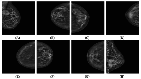
The dataset used in this paper is cited in Huang and Lin [20]. It is InBreast, which consists of eight categories for our classification task. It contains four categories for breast density with benign or malignant in the breast. In addition, the dataset contains images acquired before and after data augmentation, with a image matrix. From the 410 mammograms in the InBreast collection, 106 images representing a breast mass were selected for this study. The data expansion increased the number of mammogram images in this study to 7,632. Mammogram images with masses assigned to four different density groups and their benign or malignant status are shown in Figure 1:
- 1. Breast density is classified as 1 and breast mass as benign (Density 1+ Benign).
- 2. Breast density is classified as 1 and breast mass as malignant (Density 1+ Malignant).
- 3. Breast density is classified as 2 and breast mass as benign (Density 2+ Benign).
- 4. Breast density is classified as 2 and breast mass as malignant (Density 2+ Malignant).
- 5. Breast density is classified as 3 and breast mass as benign (Density3+ Benign).
- 6. Breast density is classified as 3 and breast mass as malignant (Density 3+ Malignant).
- 7. Breast density is classified as 4 and breast mass as benign (Density 4+ Benign).
- 8. Breast density is classified as 4 and breast mass as malignant (Density 4+ Malignant).
|
| Figure 1. Samples of images that have been used before augmentation with labels: (A) – (D) Benign; (E) – (H) Malignant |
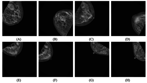
The 106 original images were pre-processed with contrast-limited adaptive histogram equalization (CLAHE) to balance and enhance the image characteristics. Figure 1 shows mammogram images with masses classified into four groups based on CLAHE processing, which was described in detail in the previous section. Figure 2 shows that the image after CLAHE processing has a clearer localization of the mass than the original image in Figure 1. There are a total of 106 original images and 106 additional images after CLAHE processing, for a total of images.
|
| Figure 2. Examples of images that have been used after augmentation with labels : (A) – (D) Benign; (E) – (H) Malignant |
3.2 Data augmentation
During the training phase, the data is constantly expanded to increase the size of the training set. The transformation can be used to enrich the data if the semantic information of the image is preserved. By solving the problem of overfitting through data enrichment, the performance of the model can be improved. Despite the fact that the CNN model has properties such as partial translation invariance, augmentation processes (i.e., translated images) often lead to a significant improvement in generalization ability [21]. Data augmentation options include a variety of methods, each with the advantage of interpreting images in different ways to highlight important features to improve performance. Data enhancement options include a variety of methods, each of which has the advantage of interpreting photographs in different ways to highlight important features and thus improve model performance. Transformations such as horizontal flipping, rotating, shearing, and zooming were evaluated as part of the augmentation evaluation.
According to Huang and Lin [20], the data is augmented by rotating it several times ( °) and flipping the actual image and images vertically and horizontally with 11 rotation angles. This technique increases the sample size and fixes the overfitting problem.
3.3 Architecture
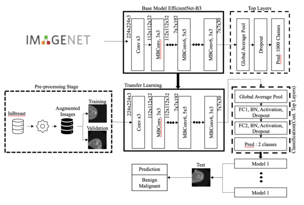
Figure 3 shows the proposed architecture based on a pre-trained EfficientNet model. We extracted features from the InBreast dataset using the pre-trained EfficentNet model [22]. This step ensures that the pre-trained EfficientNet model is able to extract and learn useful mammogram features and generalize accurately.
EfficientNets are a collection of models derived from a single base model. For simplicity, our recommended architecture shows the use of EfficientNet-B3. Two fully interconnected layers integrating stack normalization, activation, and dropout provide the output features of the pre-trained model to the proposed adapted upper layers.
|
| Figure 3. Graphical representation of the proposed architecture |
In Figure 3, each assessed EfficientNet implemented two layers of transfer learning. It was found that maintaining the dropout value of 0.3 contributed to higher precision and validation.
3.4 EfficientNet extraction of pre-trained features
EfficientNet is a collection of models (EfficientNet-B0 through EfficientNet-B7) created by extending the base network (commonly referred to as EfficientNet-B0). EfficientNet has gained popularity due to its improved predictive performance. This is achieved by applying a compound scaling method to all network parameters, including width, resolution, and depth. The compound scaling method is based on the idea that increasing any network dimension (including width, depth, or image resolution) improves accuracy, but the gain decreases as the size of the model increases. The dimensions are scaled as follows:
|
|
(1) |
|
|
(2) |
|
|
(3) |
|
|
(4) |
|
|
(5) |
where is the compound coefficient and and are the dimension-specific scaling coefficients corrected by a grid search. The network is scaled to the desired target model size after scaling the baseline network (EfficientNet-B3) using the scaling coefficients. , , and .
Observation has shown that EfficientNet is much more accurate and effective in image recognition with fewer parameters than other well-known ConvNets such as ResNet, XCeption, and Inception. These issues are further discussed in [22,28]. The main goal of this project is to demonstrate that early detection of breast cancer with EfficientNet can lead to significant improvements and potentially save a patient's life.
Since 2012, it has been shown that the success of EfficientNet has increased in direct proportion to the complexity of the models used in the ImageNet dataset. However, the vast majority of models have been shown to be computationally inefficient. The EfficientNet model, which achieved 93 percent accuracy in the ImageNet classification test with 4,978,334 parameters, can be considered a subset of the CNN models. The EfficientNet group consists of eight models with complexity ranging from B0 to B7. As the number of models increases, the number of calculated parameters remains relatively constant, but the accuracy improves exponentially. EfficientNet uses its own activation function, Swish, as opposed to the Rectifier Linear Unit (ReLU) activation function [22].
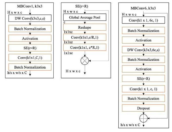
Table 2 provides comprehensive information on each layer of the EfficientNet-B3 baseline network. The feature extraction of the EfficientNet-B3 base architecture consists of multiple mobile inverted bottleneck convolutional blocks (MBConv) with integrated squeeze-and-excitation (SE), batch normalization, and swish activation [21,23-25]. EfficientNet-B3 consists of sixteen MBConv blocks, which differ in kernel size, feature map expansion phase, and reduction ratio, among others. The complete technique for the MBConv1, k, and MBConv6, k, blocks is shown in Figure 4. Both MBConv1 and MBConv6 provide for convolution in depth with a kernel size of and a step size of s. These two blocks consist of stack normalization, activation, and convolution with a kernel size of . MBConv1, k, lacks a skip connection and a dropout layer. MBConv6, k is also six times larger than MBConv1, k, and the same is true for the reduction rate in block SE, where r is fixed at four for MBConv1, k and twenty-four for MBConv6, k. MBConv6, k and MBConv6, k do not perform the same operations, but MBConv6, k uses a kernel size of and MBConv6, k uses a kernel size of .
| Stage | Operator | Resolution | #Output Feature Maps | #Layers |
|---|---|---|---|---|
| Conv | ||||
| MBConv1, k | ||||
| MBConv6, k | ||||
| MBConv6, k | ||||
| MBConv6, k | ||||
| MBConv6, k | ||||
| MBConv6, k | ||||
| MBConv6, k | ||||
| Conv & Pooling & FC |
|
| Figure 4. EfficientNet-fundamental B3's building piece |
As inputs, each MBConv block takes the values for height, width, and channel h, w, and c. C denotes the output channel for the two MBConv blocks. (MBConv stands for Mobile Inverted Bottleneck Convolution, DW Conv symbolizes convolution in depth, SE stands for squeeze excitation, and Conv stands for convolution) (a) and (c) are both Mobile Inverted Bottleneck Convolution blocks, but (c) is six times larger than (a). The representation of the squeeze excitation block is (b).
Instead of initializing the weights arbitrarily, we initialize the pre-trained weights from ImageNet in the EfficientNet model, which dramatically speeds up the training process. Since its inception, ImageNet has made significant progress in the field of image analysis, collecting approximately 14 million photos from a variety of categories. Pre-trained weights are used because the imported model already contains sufficient information about the more general features of the image domain. As a number of studies (e.g., Rajaraman et al. [26], and Narin et al. [27]) have shown, there is reason to be optimistic about the use of pre-trained ImageNet weights in modern CNN models, even when the problem to be addressed is very different from the one for which the original weights were determined. During the new training phase, the optimization technique will fine-tune the initial pre-trained weights so that researchers can fit the pre-trained model to a specific problem domain. As shown in Figure 3, the proposed architecture's approach to feature extraction uses pre-trained ImageNet weights.
3.5 Classifier
Figure 4 shows a classifier whose top layer has been updated according to the feature mining technique. Global averaging of the output features of the pre-trained EfficientNet model. To decode the classification task, a two-layer MLP (often referred to as "fully connected" (FC)) was incorporated, consisting of two neural layers representing the globally averaged attributes of the EfficientNet model (each neural layer has 512 nodes). A batch normalization, activation, and dropout layer was inserted between the FC layers.
Batch normalization significantly speeds up the training of deep neural networks and improves their stability [28]. It improves the smoothness of the optimization process, which leads to a safer and more consistent behavior of the gradient, which speeds up the training [22]. Swish was chosen as the activation function for this experiment because it is written as follows [25]:
|
|
(6) |
where the sigmoid function has the following definition: . Swish routinely outperforms other activation functions, including the best known and most successful, Rectified Linear Unit (ReLU), in a variety of difficult domains such as image classification and machine translation [29].
After activation, a dropout layer was introduced, which is one of the most successful regularization approaches to prevent overfitting and generate more accurate predictions [30]. This layer provides the ability to randomly delete FC layer nodes. In this process, all randomly selected nodes and their incoming and outgoing weights are removed. The number of randomly selected nodes dropped in each layer is determined independently of the previous layers with a probability p, which can be drawn from a validation set or a random estimate (). We maintained an attrition rate of 0.2% throughout the study. The categorical cross-entropy loss function is used to quantify the difference between the actual and predicted probabilities of a category during the training phase. The phrase "categorical cross-entropy" means:
|
|
(7) |
where is the total number of input samples and is the total number of classes, which in our case is two.
4. Result and discussions
In this part, we compare the classification performance of the proposed model with current best practices. Our software stack consists of Keras and TensorFlow. All our applications are developed in Python.
4.1 Configuration of the dataset and parameters
This section examines the distribution of the data set and the model parameters obtained from the experiment. InBreast, one of the best known freely available mammography datasets for breast cancer, was used. Since the material contains both benign and malignant breast tumors, our categorization work consists of eight categories. In addition, the dataset contains images acquired both before and after data enhancement, with an image matrix of . The distribution of images for training, validation and testing is summarized in Table 3.
| Category | Training | Testing |
|---|---|---|
| Benign | 5, 970 | 2, 394 |
| Malignant | 7, 158 | 4, 844 |
Our base model for this experiment is EfficientNet B3. The resolution of the input image varies depending on the individual base model. Higher image resolution requires the addition of more layers to capture finer patterns, increasing the number of parameters in the model. Table 4 shows the input image resolution and the total number of training parameters generated for our base model, EfficientNet B3.
| Base model | Image resolution | Total parameter size | Trainable | Non-trainable |
|---|---|---|---|---|
| EfficientNet B3 | 300x300 | 11,844,394 | 11,751,978 | 11,751,978 |
4.2 Evaluation metrics
Precision, recall, -score, confidence interval (CI), and area under the curve were used to evaluate the effectiveness of the proposed method (AUC). Precision, recall, and the score are specified precisely:
|
|
(8) |
|
|
(9) |
|
|
(10) |
|
|
(11) |
True-positive scores are represented by the symbol , whereas false-negative, true-negative, and false-positive scores are represented by the symbols , , and , respectively. The score can be a more helpful evaluation statistic due to the diversity of the benchmark dataset. The normal dataset consists of 70 photos, while the malignant dataset consists of 142 photos. In addition, a 95% confidence interval is considered a more meaningful assessment than specific performance measures. It has the potential to improve statistical power while capturing the reliability of the problem area. Finally, we represented the data by plotting the receiver operating characteristic curve and calculated the area under the receiver operating characteristic curve to measure the accuracy of the model (often abbreviated as AUC). The true positive rate (TPR)/call and false positive rate (FPR) are displayed on the ROC curve, where FPR is defined as follows:
|
|
(12) |
4.3 Prediction performance
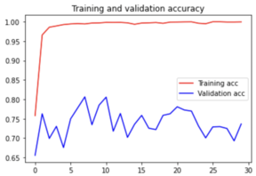
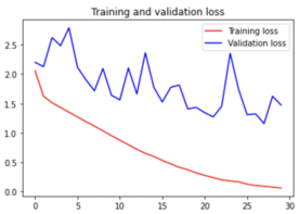
The training accuracy curve in Figure 5 indicates how well the model learns from the training data over time as the parameters of the model are changed during the training phase. Typically, training accuracy is expected to increase as the model learns more from the data, but it can also plateau as the model begins to overperform on the training data. The validation accuracy curve indicates how well the model generalizes to unseen data during training. It is important to check the validation accuracy to detect overfitting. This occurs when a model performs well on training data but poorly on new data. If the validation accuracy begins to decrease while the training accuracy continues to increase, this indicates that the model is beginning to overfit. The training and validation loss curves are similar to the accuracy curves, but they show the value of the loss function, which is the objective function that the model tries to reduce during training. The loss function evaluates the difference between the expected and actual values and indicates the model's ability to fit the data. A graph that plots the loss and accuracy curves for training and validation is a valuable tool for monitoring the performance of a machine learning model during training. It can help detect overfitting, identify the optimal model architecture, and optimize training hyperparameters.
| ||||
| Figure 5. EfficientNet B3 accuracy and loss curve |
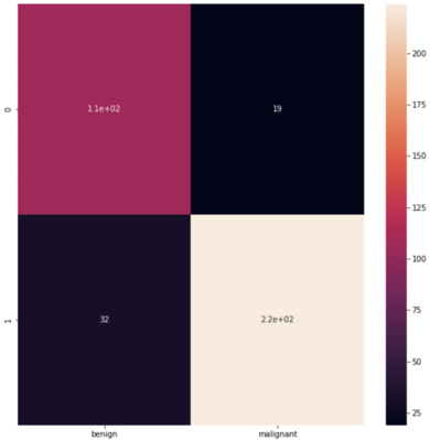
Accuracy was determined using a 95% confidence interval (CI). A small confidence interval indicates higher accuracy, while a large confidence interval indicates the opposite. As you can see, the confidence interval is narrow when augmentation is not present and large when it is. The confusion matrix for Efficient Net Pre-trained Weights is also shown in Figure 5. We believe that our proposed architecture is compelling for detecting benign cancer cells in mammography nodules. This may be because its features perform better in detecting benign cancer cells than malignant cells.
We implemented the model without making any changes. As can be seen in Table 5, EfficientNet-B3 has a recognition and score of 87 percent.
| Pre-trained Weight | Precision (%) | Recall (%) | F1-Score (%) | Accuracy (%) |
|---|---|---|---|---|
| EfficientNet-B3 | 77.4 | 85.3 | 81.2 | 86.5 |
In this study, we evaluated the effectiveness of our proposed classification model using a confusion matrix in Figure 6 with the following values: 110 true positives, 32 false positives, 19 false negatives, and 220 true negatives. The model achieved 86.5 percent accuracy, 77.4 percent precision, 85.3 percent recognition, and 81.2 percent . Despite occasional misclassifications, the model showed excellent overall performance with high accuracy, balanced recognition, and precision. These results indicate that the proposed model could be a useful categorization tool for a variety of domains. Further studies can be conducted to investigate the generalizability of the model to different datasets and domains.
|
| Figure 6. Confusion matrix of efficientNet B3 |
5. Conclusions
In this paper, an improved convolutional network architecture for breast cancer nodule detection in mammography is presented. The goal of this work is to show that EfficientNet is one of the best models for image recognition in terms of the minimum parameters used, although other researchers claim that another technique is more accurate. Experiments were performed to evaluate the performance of convolutional neural networks using EfficientNet on InBreast datasets with benign and malignant tumor cells, and it was shown that EfficientNet significantly improves accuracy compared to other approaches. It is believed that integrating EfficientNet into breast cancer screening will help save lives and increase survival rates. Although our proposed model is 86.5 percent less accurate than others, it can be confidently said that EfficientNet is a serious competitor to other methods. This shows that EfficientNet can be improved over time and will continue to be a competitive solution for other systems.
It is worth noting that according to current CNN application research, performance increases as the number of available and trained samples increases. In addition, it is important to focus on the early stages where these methods may perform poorly, and a comprehensive analysis of these methods, taking into account the patient's disease progression, is critical. While EfficientNet is used as a baseline model by only a few authors, the purpose of this study is to highlight EfficientNet as a baseline model that should be considered in the future.
Funding Statement
Part of this work was supported by the SASMEC Research Grant (SRG)- SRG21-011-0011
Conflict of Interest
The authors declare that they have no conflicts of interest to report regarding the present study.
References
[1] Kasban H., El-Bendary M.A.M., Salama D.H. A comparative study of medical imaging techniques. Int. J. Inf. Sci. Intell. Syst., 4(2):37–58, 2015. [Online]. Available: https://www.researchgate.net/publication/274641835.
[2] Khan S.U., Islam N., Jan Z., Ud Din I., Rodrigues J.J.P.C. A novel deep learning based framework for the detection and classification of breast cancer using transfer learning. Pattern Recognit. Lett., 125:1–6, 2019. doi: 10.1016/j.patrec.2019.03.022.
[3] Saba L. et al. The present and future of deep learning in radiology. Eur. J. Radiol., 114:14–24, 2019. doi: 10.1016/j.ejrad.2019.02.038.
[4] Yunus M., Ahmed N., Masroor I., Yaqoob J. Mammographic criteria for determining the diagnostic value of microcalcifications in the detection of early breast cancer. J. Pak. Med. Assoc., 54(1):24–29, 2004.
[5] Hussain S.I., Ruza N. Automated deep learning of COVID-19 and pneumonia detection using google autoML. Intelligent Automation & Soft Computing, 31(2):1143-1156, 2022.
[6] Niazi M.K.K., Parwani A.V., Gurcan M.N. Digital pathology and artificial intelligence. Lancet Oncol., 20(5):e253–e261, 2019. doi: 10.1016/S1470-2045(19)30154-8.
[7] Azman B.M., Hussain S.I., Azmi N.A., Abd Ghani M.Z.A., Norlen N.I.D. Prediction of distant recurrence in breast cancer using a deep neural network. Revista Internacional de Métodos Numéricos para Cálculo y Diseño en Ingeniería, 38(1), 12, 2022.
[8] Shen L., Margolies L.R., Rothstein J.H., Fluder E., McBride R., Sieh W. Deep learning to improve breast cancer detection on screening mammography. Sci. Rep., 9(1):1–12, 2019. doi: 10.1038/s41598-019-48995-4.
[9] Rodriquez-Ruiz A., et al. Detection of breast cancer with mammography: Effect of an artificial intelligence support system. Radiology, 290(2):305-314, 2019. doi: 10.1148/radiol.2019190372.
[10] Ragab D.A., Sharkas M., Marshall S., Ren J. Breast cancer detection using deep convolutional neural networks and support vector machines. PeerJ, 7:e6201, 2019, doi: 10.7717/peerj.6201.
[11] Wang J., Yang X., Cai H., Tan W., Jin C., Li L. Discrimination of breast cancer with microcalcifications on mammography by deep learning. Sci. Rep., 6, 27327, 2016. doi: 10.1038/srep27327.
[12] DeSantis C.E., Ma J., Goding Sauer A., Newman L.A., Jemal A. Breast cancer statistics, 2017, racial disparity in mortality by state. CA. Cancer J. Clin., 67(6):439–448, 2017.
[13] American Cancer Society. What is breast cancer? Am. Cancer Soc. Cancer Facts Fig., Atlanta, Ga Am. Cancer Soc., 1–19, 2017.
[14] Zhang Y.D., Satapathy S.C., Guttery D.S., Górriz J.M., Wang S.H. Improved breast cancer classification through combining graph convolutional network and convolutional neural network. Inf. Process. Manag., 58(2), 102439, 2021. doi: 10.1016/j.ipm.2020.102439.
[15] Albalawi U., Manimurugan S., Varatharajan R. Classification of breast cancer mammogram images using convolution neural network. Concurr. Comput., 34(13), e5803, 2022. doi: 10.1002/cpe.5803.
[16] Maqsood S., Damaševičius R., Maskeliūnas R. TTCNN: A breast cancer detection and classification towards computer-aided diagnosis using digital mammography in early stages. Appl. Sci., 12(7):3273, 2022. doi: 10.3390/app12073273.
[17] Tsochatzidis L., Koutla P., Costaridou L., Pratikakis I. Integrating segmentation information into CNN for breast cancer diagnosis of mammographic masses. Comput. Methods Programs Biomed., 200, 105913, 2021. doi: 10.1016/j.cmpb.2020.105913.
[18] Salama W.M., Aly M.H. Deep learning in mammography images segmentation and classification: Automated CNN approach. Alexandria Eng. J., 60(5):4701–4709, 2021. doi: 10.1016/j.aej.2021.03.048.
[19] Tsochatzidis L., Costaridou L., Pratikakis I. Deep learning for breast cancer diagnosis from mammograms — A comparative study. J. Imaging, 5(3), 37, 2019. doi: 10.3390/jimaging5030037.
[20] Huang M.L., Lin T.Y. Dataset of breast mammography images with masses. Data in Brief., 31, 105928, 2020.
[21] Tan M., et al. Mnasnet: Platform-aware neural architecture search for mobile. Proc. IEEE Comput. Soc. Conf. Comput. Vis. Pattern Recognit., pp. 2815–2823, 2019.
[22] Tan M., Le Q.V. EfficientNet: Rethinking model scaling for convolutional neural networks. 36th Int. Conf. Mach. Learn. ICML 2019, pp. 10691–10700, 2019.
[23] Sandler M., Howard A., Zhu M., Zhmoginov A., Chen L.C. MobileNetV2: Inverted residuals and linear bottlenecks. In Proceedings of the IEEE Conference on Computer Vision and Pattern Recognition, pp. 4510–4520, 2018.
[24] Hu J., Shen L., Sun G. Squeeze-and-excitation networks. In Proceedings of the IEEE Conference on Computer Vision and Pattern Recognition, pp. 7132–7141, 2018.
[25] Zoph B., Le Q.V., Ramachandran P. Searching for activation functions. 6th Int. Conf. Learn. Represent. ICLR 2018 - Work. Track Proc., pp. 1–13, 2018.
[26] Rajaraman S., Siegelman J., Alderson P.O., Folio L.S., Folio L.R., Antani S.K. Iteratively pruned deep learning esembles for COVID-19 detection in chest X-rays. IEEE Access, 8:115041–115050, 2020.
[27] Narin A., Kaya C., Pamuk Z. Automatic detection of coronavirus disease (covid-19) using x-ray images and deep convolutional neural networks. Pattern Anal. Appl., 24(3):1207-1220, 2021.
[28] Luz E. et al. Towards an effective and efficient deep learning model for COVID-19 patterns detection in X-ray images. Res. Biomed. Eng., 38:149–162, 2022.
[29] Vinod N., Hinton G E. Rectified linear units improve restricted Boltzmann machines. Proceedings of the 27th International Conference on Machine Learning, Haifa, Israel, 2010.
[30] Srivastava N., Hinton G., Krizhevsky A. Salakhutdinov R. Dropout: A simple way to prevent neural networks from overfitting. J. Mach. Learn. Res., 15:1929–1958, 2014.Document information
Published on 01/09/23
Accepted on 25/07/23
Submitted on 16/03/23
Volume 39, Issue 3, 2023
DOI: 10.23967/j.rimni.2023.08.002
Licence: CC BY-NC-SA license
Share this document
Keywords
claim authorship
Are you one of the authors of this document?
