Iber v3. Reference manual and GUI. Large wood transport calculation module

Abstract

Large wood plays a vital role in river systems, shaping habitats and supporting biodiversity. However, during floods, large wood transport can threaten infrastructure and communities. Traditional flood models often overlook wood material, despite its natural presence in rivers. To address this gap, the calculation module Iber-Wood was developed and integrated into the Iber model. Iber-Wood combines the Eulerian Iber 2D hydrodynamics with a Lagrangian model to simulate wood as dynamic elements. The model accounts for wood-flow-sediment, wood-wood, wood-infrastructure, and wood-terrain interactions, using two-way coupling. It has been validated with flume experiments and applied to various real rivers using field data. Applications include studying wood-sediment-flow dynamics and bridge-related wood accumulation. Though deterministic, Iber-Wood enables scenario testing and hypothesis exploration for complex wood dynamics.

Keywords: large wood, clogging, driftwood, woodjam, wood regime.

Resumen

El material leñoso de gran tamaño (troncos, restos de árboles, ramas y raíces) en los ríos desempeña un papel vital en los sistemas fluviales, configurando hábitats y sustentando la biodiversidad. Sin embargo, durante las inundaciones, el transporte de madera puede amenazar infraestructuras y comunidades. Los modelos de inundación tradicionales pasan por alto el transporte de material de madera, a pesar de su presencia natural en los ríos. Para abordar esta problemática, se desarrolló el módulo de cálculo Iber-Wood, que está completamente integrado en Iber. Iber-Wood combina la hidrodinámica euleriana 2D de Iber con un modelo lagrangiano para simular la madera como elementos dinámicos. El modelo considera las interacciones madera-flujo-sedimento, madera-madera, madera-infraestructura y madera-terreno, utilizando acoplamiento bidireccional. Se ha validado con experimentos de canal y se ha aplicado a varios ríos reales utilizando datos de campo. Las aplicaciones incluyen el estudio de la dinámica del flujo madera-sedimento y la acumulación de madera relacionada con los puentes. Aunque determinista, Iber-Wood permite la exploración de escenarios e hipótesis para dinámicas complejas de la madera.

Palabras clave: material leñoso, obstrucción, madera flotante, acumulación de madera, bloqueo de puente, régimen de la madera.

1. Introduction

1.1. Wood transport in rivers and wood transport modelling

Wood significantly influences the hydraulics, morphodynamics, and ecology of fluvial systems, playing a key role in biodiversity support. However, during floods, large wood transport can pose substantial risks to infrastructure and communities. While models for flows and floods in mountain rivers have existed for decades, they often exclude organic material [1], despite forested catchments naturally contributing substantial wood to rivers (e.g., uprooted trees and trunks). To address this, Iber-Wood was developed in 2013 [2] and fully integrated into the Iber modelling framework [3,4,5].

Iber-Wood couples 2D hydrodynamics and morphodynamics (Eulerian) with a Lagrangian discrete element model representing wood as cylindrical elements (with/without roots). These elements respond to hydrodynamic forces, enabling them to float, slide or drag, collide (inelastically), deposit, or remobilize. They interact with each other, with infrastructures, and the topography. The model is two-way coupled, meaning that the presence of wood modifies hydrodynamics by introducing a drag component into the Saint-Venant equations, thereby influencing morphodynamic processes; and the hydrodynamics govern the motion of wood. For details regarding the governing equations please see the reference [6].

The model has been validated with flume experiments and applied to several rivers with field data [7,8,9,10,11]. It has been used to study flow-wood-sediment interactions, where wood input alters sediment transport dynamics, and erosion can remobilize deposited wood [3,12]. Applications include assessing wood accumulation at bridges and associated scour/aggradation [13,14].

Despite its capabilities, Iber-Wood remains a deterministic model aiming at simulating a quasi-stochastic process, inherently subject to uncertainties. Accurate site-specific data and detailed observations are essential for model calibration and validation. Nevertheless, its main strength lies in the capacity to explore hypotheses and simulate multiple scenarios, offering valuable insights into complex, rarely observable wood dynamics.

Please read the Iber documentation (i.e., quick user guide, hydraulic reference manual, tutorials and scientific papers) available at www.iberaula.es for details. This document does not explain how to use Iber and assumes that the modeller is already familiar with the software.

The Iber online manual can be found here:

• Iber v3. Reference manual and GUI of the new implementations (in Spanish)

As well as tutorials and benchmarks:

• Iber applications basic guide
• Benchmarking of the Iber capabilities for 2D free surface flow modelling
• River flood hazard modelling and management

1.2. This manual and Iber-Wood Installation

This manual is a quick-start user guide for Iber version 3.4 or later. Further information, such as a description of the governing equations and applications, can be found in the References.

Iber-Wood is a calculation module (Plugin) of Iber, a freely distributed software for the simulation of free surface water flows. The interface of Iber is based on GiD, a pre- and post-process tool for multidimensional problem types. Therefore, the first step is to download and install Iber, available from: https://www.iberaula.es/

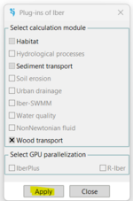
Once installed, Iber Wood can be activated in the menu Iber tools >> Plug-ins..., as shown in Figure 1, and the Wood Transport can be turned on in the Data Window.

Figure 1: Activation window and general options for wood transport

Problem Data > Wood > Extra Results: additional results can be displayed; they have been used by the model developers mostly and are not needed for most users.

2. Pre-process: setting up a model

Before defining the initial and/or boundary conditions for wood transport, the model setup must follow several key steps:

• Create or import the computational geometry (optional)
• Generate the computational mesh
• Define input parameters (e.g., bed roughness, turbulence model)
• Specify boundary (inflow/outflow) and initial conditions
• Configure problem settings (e.g., simulation duration, numerical scheme parameters, additional module requirements)

Detailed guidance on each of these steps can be found in the corresponding model manuals.

It is essential to ensure that all necessary data is available for running, validating, and calibrating the model.

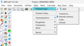
If a model has been built with an older version of Iber or Iber-Wood is recommended to transform it to the latest version as shown in fFgure 2:

Figure 2: Transform tool for older projects

2.1. Wood input parameters and initial conditions

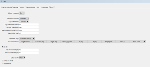
The wood computation parameters, characteristics and initial conditions can be added in the Problem Data menu, Wood (Fig.3):

Figure 3: Wood data window with input parameters and initial conditions

Use the help button, place the mouse on some parameters and options to read more details and descriptions.

Kinematic or dynamic approach

The incipient motion of a log is fully dynamic, and it is based on the balance of forces (i.e., gravity, friction and drag forces) acting on the centre of mass of the log (i.e., wood piece). However, the velocity of the log can be simulated using two different approaches: kinematic and dynamic. In the first one, the kinematic approximation, log density, log diameter and water depth are used to define the transport regimes: resting, floating, or by traction (i.e., sliding). If the log floats ,the velocity is the same as the flow velocity, unless turbulence is included in the calculation (see section about turbulence). If the log slides on the river bed , the log velocity is different fromthe flow velocity.

The dynamic approximation uses the equations describing the movement of a rigid solid to calculate log velocity at each time step. In the case of the dynamic framework, the drag coefficient (Cd) used in the governing equations, has a strong influence on the resulted log velocity.

We recommend using the kinematic approach, as it has undergone more extensive validation compared to the alternative dynamic method. Its reliability has been demonstrated across a wider range of scenarios and case studies.

Drag Coefficient

The drag coefficient is an important parameter in log velocity computations. This coefficient varies with the log shape, its position in the stream and Reynolds number. Drag coefficient values for many different shapes of bodies have been studied extensively. Here we reported some values:

Drag Coefficient Cd	Reference	Comments
1.2	Brooks et al., 2006	Real logs
1.41	Bocchiola et al., 2006	Dowels in flume
0.8	Mazzorana et al., 2011
0.7-0.9	Shields and Gippel, 1995
1.5	Alonso, 2004
0.4-1.2	Gippel et al., 1996
1	Fischerich and Morrow, 2000
1.54	Boothroyd et al., 2016	Complex vegetation
Up to 4	Hui et al., 2010	Leafy shrubs

A constant value of 1.2 is suggested by default in the model but this value can be changed by the modeller and must be calibrated.

Additionally, a variable drag coefficient with log orientation (θ) can also be used. The equation proposed by Gippel (1992) is implemented in the model:

Cd=1.1173 - 5.28x10^-2· Ɵ + 1.4385x10^-3· Ɵ² - 9.7668x10^-6· Ɵ³

Friction Coefficient

The other input parameter is the friction coefficient between the wood and the river bed. This value may significantly affect the movement of sliding logs; therefore, it must also be selected with caution.

A value equal to 0.47 is used by default as suggested by Ishikawa (1989), although higher values were proposed by other authors:

Friction coefficient µbed	Reference
0.47	Ishikawa, 1989
0.62	Buxton, 2010
0.2	Bocchiola et al., 2006
1	Mazzorana et al., 2011

Additionally, the friction coefficient can be calculated as µ_bed=tan(Ø), where Ø is the internal friction angle of soil.

The wall bouncing angle

The wall bouncing angle is used to compute log motion when logs touch a wall or a steep bank. When the incidence angle (i.e., the angle between the log and the boundary) is lower than this wall bouncing angle the movement of the log is treated as sliding or gliding parallel to the wall. On the other hand, if the incidence angle is higher, the log bounces off and changes its trajectory suddenly.

Based on our own observations, we suggest a wall bouncing angle equal to 45º (0.78 radians).

Restitution Coefficient

The Restitution Coefficient is used to compute the log-log interactions. Log-log interactions are considered as rigid bodies' elastic collisions when the Restitution Coefficient is equal to 1. Collisions might be inelastic by changing the value of the restitution coefficient.

Wood density

Wood density is used to calculate the initial motion, and it influences the way logs move (floating or by traction). Wood density varies as a function of several factors, including tree species, wood type (proportion of early to late wood), tree age (and proportion of heartwood to sapwood), decay status, and moisture content.

Therefore, wood density needs to be chosen with caution.

Some values reported in the literature are compiled in this table:

Wood density value or ranges (kg/m3)	Comments	Reference
440-630	Dry wood	Haga et al., 2007
1150-1170	Wet wood
1058	Wet (saturated) wood	Buxton, 2010
750		Merten et al., 2010
693±102	Abies (green wood)	Ruiz-Villanueva et al. (2016c) [15]
794±79	Acer (green wood)
874±73	Alnus (green wood)
816±70	Fraxinus (green wood)
793±118	Populus (green wood)
843±150	Quercus (decayed)
789±10	Salix (decayed)
800	Green wood
660	Decayed instream wood
850-950	Large Alders	Ruiz-Villanueva et al. (2016b,d) [9,16]
400-700	Willows (Salix)

When logs are in contact with the water, they gain moisture, which influences the wood density. Based on experimental experience [15], wood density may vary with time following the equation:

ρ_f = ρ_i∙e^K·t

Where ρ_f is the final wood density, ρ_i is the initial wood density, K is a constant and t is time.

For short time periods (i.e., flash floods), the variability in wood density due to moisture absorption might not be significant and can be neglected.

Wood initial conditions or deposited logs

Deposited logs, or initial conditions for wood, can be defined by specifying the following parameters for each log at a given time step (typically the initial one):

• Position: x and y coordinates of the log’s centre of mass
• Orientation: angle relative to the flow direction (in radians)
• Length (m) and diameter (m)
• Wood density (kg/m³)

Each log must be assigned a unique identification number.

If variable wood density is considered, the table also requires the initial density and a variation exponent (K) for each log.

Input data can be copied and pasted directly from a text file or an Excel spreadsheet.

Wood with roots

If logs include roots, this option must be enabled. Root systems are modelled as attached cylindrical elements [11], defined by their maximum diameter and width. A reduction coefficient is then applied to adjust the effective size of each rootward.

The presence of roots affects the friction, gravity and drag forces acting on the log. The main effect of the presence of roots is the increase in resisting forces, as roots may contact the riverbed, increasing the friction, depending on the buoyancy. Furthermore, rooted pieces are more likely to rotate, with the roots pointing upstream [17]. Our approximation only considers the frontal area of the rootwad, which has been proven to be the relevant parameter influencing the motion of wood with roots [18].

2.2. Wood boundary conditions and wood gauges

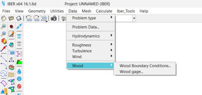
Wood inlet boundary conditions and wood gauges can be assigned to the domain in the Data menu (Fig.4), and inlet boundary and initial conditions too (Fig.5).

Figure 4: Wood inlet boundary conditions and wood gauges menus

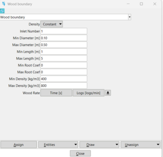
Figure 5: Inlet wood boundary conditions menu

Based on the modeller's knowledge of the fluvial corridor, riparian vegetation, and wood availability, ranges of maximum and minimum log lengths, diameters, root size and density of wood are defined. Stochastic variations of these parameters, together with the angle, are used to characterise each log entering the model.

Inlet boundary conditions (i.e., wood rate or flux: number of logs entering the simulation; Fig.6) can be assigned to the simulation domain boundaries (as many as needed), specifying a number of wood pieces per minute and their main characteristics (i.e., size and density). If more than one wood inlet is added, they should be numbered (e.g., Inlet number: 1, 2, 3…., n).

• Wood inlet boundary conditions must be located at boundaries with inlet boundary conditions of flow
• Wood rate is distributed proportionally to discharge across the inlet boundary
• The entry log position along the boundary is randomly selected, but its probability is proportional to discharge
• The end of the wood flux must be indicated with a value equal to 0

Figure 6: inlet boundary wood rate window

Wood gauges can be added at any place in the domain (once the mesh has been created), as a line perpendicular to the channel, to obtain the fluxes of wood in terms of logs (in number and volume) crossing the gauge at each time step (Fig. 7).

Figure 7: Wood gauge window

Make sure the coordinates are entered correctly (edit them in the start and end points manually if needed, and be aware that GID writes these numbers in scientific notation).

2.3. Turbulence

Iber includes several turbulence models (i.e., constant viscosity coefficient, parabolic, mixing length and k–ε), but when considering the influence of turbulence on wood transport, only the Rastogi–Rodi k–ε model can be used so far (Fig.8). If turbulence is activated in the calculation, wood velocity is then calculated using the fluctuations of the turbulent flow velocity, which basically means introducing a random component into the motion of logs transported by a turbulent flow. In this way, identical logs dropped into the same spot may end up in different places.

Figure 8: Turbulence mode activated, compatible with wood transport.

Please check the Iber documentation to learn more about the turbulence module.

2.4. Infrastructures

Iber-Wood reproduces interactions between wood logs and infrastructures, computing whether a log can pass under or above a bridge deck, weir or gate, or become trapped by the structure. Interactions between wood and culverts or lids are not yet implemented.

Please check the Iber documentation to learn how to add bridges, piers, weirs, gates, etc.

3. Computation

To launch a computation, all the input parameters must be set.

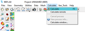
The computation is starting with the menu Calculate (Fig.9).

Please, read the Iber documentation regarding the calculation parameters, the results selection, etc.

Figure 9: The menu Calculate

View process info shows the progress of the calculation and the inlet and outlet discharge.

4. Postprocess

Once the computation is over, or even during the simulation process, the post-process interface can be accessed to visualise and analyse the results.

Switching between pre-processing and postprocessing interfaces can be done in the menu:

File > Post-process.

Or using the icon in the upper right:

Iber provides multiple options to visualise and analyse the results; please check the Iber documentation.

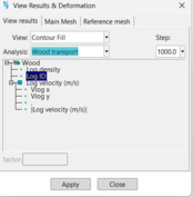
In the case of Iber-Wood, results can be displayed and visualised using the View Results menu (Fig.10).

Figure 10: View Results menu for wood

Different options are available to visualise the wood transport results at each time step: log visualisation (as lines), log density, number of logs, log velocity, etc. Wood simulation´s results are also written in different text files (.rep) created during the computation inside the project folder. These files can be opened with a text editor.

5. Output files

All output files are created inside the project folder in a folder named Wood (Fig.11).

Figure 11: Results folder named Wood and created result files

The first output file created when running Iber-Wood is the one named wood.rep

This file shows all results from the wood transport simulation written for each time step and each log: Time (s); ilog; Name; X; Y; Angle; Length (m); Diameter (m); Vx,log (m/s); Vy,log (m/s); Vx (m/s); Vy (m/s); A_log; A_sub; Density (kg/m3); Manning; Depth (m); Elevation (m); Cd; Case; Travelled dist. (m); Straight dist. (m); Root_coef.

• Ilog is the number of logs present in the simulation; this is not the number assigned to each log and changes with time
• The ID of the log is the name of the log, which remains constant over time

The coordinates of the centre of mass are written together with the angle (in radians), its size (length and diameter in meters), log velocity (in the two directions, X and Y), the flow velocity of the element where the log´s centre of mass is located, the area of the log, the submerged area of the log (both in m²), the log´s density, the value of the manning roughness of the element where the log´s centre of mass is located, the water depth in meters and its elevation (m a.s.l.) of that element, and the log drag coefficient (Cd). Case refers to the state of the log (e.g., submerged, or emerged), but it is information for developers only. The actual and straight distances travelled by the log are also provided, and the root coefficient in the case of logs with roots.

At the end of the file a summary (Figure 12) is computed with the total number of supplied logs is together with the number of exited logs (outside the domain), logs deposited (only when log velocity=0 m/s) within the studied domain and number of moving logs within the domain (i.e., log velocity not equal to 0).

Figure 12: Summary of total number of supplied logs is together with the number of exited logs (outside the domain), logs deposited (only when log velocity=0 m/s) within the studied domain and number of moving logs within the domain (i.e., log velocity not equal to 0)

Wood_gauges.rep

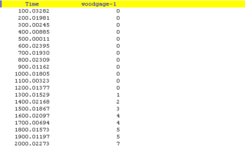
This file (Fig. 13) contains the computation of a number of logs (cumulative) passing through the wood gauge (if created in the pre-process) at each time step.

Figure 13: Wood_gauges.rep file

WoodVol_gauges.rep

This file is similar to the previous one, but instead of recording the number of logs, the volume of logs is written (in m³).

Other output files

proceso.rep: This output file contains the information about the progress of the computation. It is the same information as shown in the View process info (Calculation Window).

6. Applications

The Iber-Wood model has been applied in a variety of case studies and theoretical investigations addressing several key aspects of large wood dynamics in fluvial environments. These applications include the analysis of large wood accumulation at bridges [19], the influence of large wood on river morphology and morphodynamics [20], and hazard and risk assessment scenarios associated with the transport of wood during floods and flash floods [21,22,23]. Additionally, the model has been employed to examine the role of secondary currents in bended channels in the motion of large wood [24].

References

[1] Ruiz-Villanueva, V. 2024. Numerical modelling of wood transport processes in mountain rivers and torrents: a review. Fachtagung Wildbäche 2024: Modellierung von Wildbachprozessen 33–40. WSL Berichte 155, Kompetenzbereich Wasserbau der OST – Ostschweizer Fachhochschule und der Forschungsgruppe Wildbäche und Massenbewegungen der Eidg. Forschungsanstalt WSL, http://doi.org/10.55419/wsl:37771

[2] Ruiz-Villanueva, V., Bladé, E., Sánchez-Juny, M., Marti-Cardona, B., Díez-Herrero, A., Bodoque, J.M., 2014a. Two-dimensional numerical modeling of wood transport. J. Hydroinformatics 16, 1077–1096. https://doi.org/10.2166/hydro.2014.026

[3] Bladé, E., Cea, L., Corestein, G., Escolano, E., Puertas, J., Vázquez-Cendón, E., Dolz, J., and Coll, A. 2014. Iber: herramienta de simulación numérica del flujo en ríos, Rev. Int. Métodos Numéricos para Cálculo y Diseño en Ing., 30, 1–10, http://dx.doi.org/10.1016/j.rimni.2012.07.004

[4] Sanz-Ramos, M., Cea, L., Bladé, E., López-Gómez, D., Sañudo, E., Corestein, G., García-Alén, G., Aragón-Hernández, J. 2022. Iber v3. Reference manual and user’s interface of the new implementations, CIMNE, https://doi.org/10.23967/iber.2022.01

[5] Sanz-Ramos, M., Sañudo, E., Cea, López-Gómez, D., García-Feal, O., Cea, L., Bladé, E. 2025. Evolution of the two-dimensional numerical modelling of free surface flows through Iber software. Ingenieria del Agua 29.2. 114-131. https://doi.org/10.4995/ia.2025.23259

[6] Ruiz Villanueva, V., Bladé Castellet, E., Díez-Herrero, A., Bodoque, J. M., Sánchez-Juny, M. 2014b. Two-dimensional modelling of large wood transport during flash floods. Earth Surface Processes and Landforms, 39(4), 438–449. https://doi.org/10.1002/esp.3456

[7] Ruiz-Villanueva, V., Bodoque, J.M., Díez-Herrero, a., Bladé, E., 2014c. Large wood transport as significant influence on flood risk in a mountain village. Nat. Hazards 74, 967–987. https://doi.org/10.1007/s11069-014-1222-4

[8] Ruiz-Villanueva, V., Piégay, H., Gurnell, A.M., Marston, R.A., Stoffel, M., 2016a. Recent advances quantifying the large wood dynamics in river basins: New methods and remaining challenges. Rev. Geophys. 54, 611–652. https://doi.org/10.1002/2015RG000514

[9] Ruiz-Villanueva, V., Wyzga, B., Zawiejska, J., Hajdukiewicz, M., Stoffel, M., 2016b. Factors controlling large-wood transport in a mountain river. Geomorphology 272, 21–31. https://doi.org/10.1016/j.geomorph.2015.04.004

[10] Ruiz-Villanueva, V., Wyżga, B., Mikuś, P., Hajdukiewicz, M., Stoffel, M., 2017. Large wood clogging during floods in a gravel-bed river: the Długopole bridge in the Czarny Dunajec River, Poland. Earth Surf. Process. Landforms. https://doi.org/10.1002/esp.4091

[11] Ruiz-Villanueva, V., Gamberini C., Bladé, E., Stoffel, M., Bertoldi, W., 2020. Numerical modelling of instream wood transport, deposition and accumulation in braided morphologies under unsteady conditions: sensitivity and high-resolution quantitative model validation. Water Resour. Res. https://doi.org/10.1029/2019WR026221

[12] Bladé E., Ruiz-Villanueva V., M Sánchez-Juny. 2016. Strategies in the 2D numerical modelling of wood transport in rivers. River Flow 2016 – Constantinescu, Garcia & Hanes (Eds), Taylor & Francis Group, London, ISBN 978-1-138-02913-2. https://hdl.handle.net/2117/89229

[13] Mazzorana, B., Bahamondes Rosas, D., Montecinos, L., Ruiz-Villanueva, V., Rojas, I. 2023. Explorando la respuesta hidrodinámica de un río altamente perturbado por erupciones volcánicas: el Río Blanco, Chaitén (Chile). Ingeniería Del Agua, 27(2), 73–92. https://doi.org/10.4995/ia.2023.18866

[14] Valera-Prieto, Ll., Sanz-Ramos, M., Ruiz-Villanueva, V. 2024. Modelling of morphodynamics and large wood transport during the 2019 flash flood in the Francolí River (Tarragona). XI Congreso Geológico de España 2024, Ávila (Spain). Link

[15] Ruiz-Villanueva, V., Piégay, H., Gaertner, V., Perret, F., & Stoffel, M. 2016c. Wood density and moisture sorption and its influence on large wood mobility in rivers. Catena, 140, 182–194. https://doi.org/10.1016/j.catena.2016.02.001

[16] Ruiz-Villanueva, V., Wyżga, B., Mikuś, P., Hajdukiewicz, H., Stoffel, M., 2016d. The role of flood hydrograph in the remobilization of large wood in a wide mountain river. J. Hydrol. 541, 330–343. https://doi.org/10.1016/j.jhydrol.2016.02.060

[17] Comper, T., Lorenzo Picco, Ernest Bladé Castellet, Ruiz-Villanueva, V. 2018. Numerical modelling of large wood dynamics in the braided Piave River (Italy): the important role of roots. 5th IAHR Europe Congress — New Challenges in Hydraulic Research and Engineering, DOI:10.3850/978-981-11-2731-1_210-cd. Link

[18] Ghaffarian Roohparvar, H., Lopez, D., Mignot, E., Piégay, H., Riviere, N. 2020. Dynamics of floating objects at high particulate Reynolds numbers. Physical Review Fluids. 5. https://10.1103/PhysRevFluids.5.054307

[19] De Cicco, P.N.; Paris, E., Ruiz-Villanueva, V., Solari, L.; Stoffel, M. 2018. Wood accumulation at bridge piers: a review. River Research and Applications 34, 617-628. https://doi.org/10.1002/rra.3300

[20] Ruiz-Villanueva, V., Wyzga, B., Hajdukiewicz, H., Stoffel, M., 2016e. Exploring large wood retention and deposition in contrasting river morphologies linking numerical modelling and field observations. Earth Surf. Process. Landforms 41, 446–459. https://doi.org/10.1002/esp.3832

[21] Quiniou, M., Piton, G., Villanueva, V.R., Perrin, C., Savatier, J., Bladé, E. 2022. Large Wood Transport-Related Flood Risks Analysis of Lourdes City Using Iber-Wood Model. In: Gourbesville, P., Caignaert, G. (eds) Advances in Hydroinformatics. Springer Water. Springer, Singapore. https://doi.org/10.1007/978-981-19-1600-7_31

[22] Sanz-Ramos, M., Valera-Prieto, Ll., García Feal, O., Furdada, G., Bladé, E., Ruiz-Villanueva, V. 2024. Numerical modelling of morphodynamics and large wood transport during flash floods in two Mediterranean Rivers. Conference: Wood in World Rivers 5, Gaspé, Canada. Link

[23] Mazzorana B., Ruiz-Villanueva V., Marchi L., Cavalli M., Gems B., Gschnitzer T., Mao L., Iroumé A., Valdebenito G. 2018. Assessing and mitigating large wood-related hazards in mountain streams: recent approaches. Journal of Flood Risk Management 11: 207-222. https://doi.org/10.1111%2Fjfr3.12316

[24] Innocenti, L., Bladé, E., Sanz-Ramos, M., Ruiz-Villanueva, V., Solari, L., Aberle, J. 2023. Two-dimensional numerical modeling of large wood transport in bended channels considering secondary current effects. Water Resources Research, 59, e2022WR034363. https://doi.org/10.1029/2022WR034363