Influence of residual stress models prescribed in design codes for steel I-section behavior

Abstract

Non-uniform cooling of steel cross-sections during the manufacturing process generates a state of residual stresses in the cross-section. Design codes describe the distribution of these stresses in different ways. This work aims to numerically investigate the influence of these models on the behavior of bare steel and steel-concrete composite sections by the curves: flexural stiffness-bending moment, moment-curvature and yield curves (initial and full yield). These procedures are important for the study of the simplified curves used in some methodologies of the refined plastic hinge method (RPHM) analysis. The study will use the strain compatibility method (SCM), where, if the axial strain of the cross-section point is known, the section stiffness is obtained using the tangential Young's modulus derived from the materials constitutive relationship. A fiber discretization algorithm is applied and the residual stresses are explicitly inserted into the fibers automatically. The methodology was calibrated using the moment-curvature relationship and the flexural stiffness-bending moment curve. These results were numerically stable and good convergence with literature data was obtained. In general, the residual stress model of the American standard (AISC, 2016) defines a larger elastic region within the interaction diagrams then European model (CEN, 2005). The results obtained showed that the initial yield curves for steel I-sections under minor axis bending require revision for application to RPHM, mainly due to the loss of symmetry in relation to the $M$ axis in the normal force-bending moment ($NM$) interaction diagram.

Keywords: Steel I-sections, residual stresses, design codes, moment-curvature relationship, yield curves

1. Introduction

In steel structures analysis some factors, such as geometric imperfections and residual stresses, can contribute to the reduction of the structural system’s bearing capacity. Residual stresses occur from unequal cooling of the parts, after the rolling, cutting, welding processes or mechanical operations (in case of cold-formed sections) [1]. According to Alvarenga [2], several laboratory tests allowed the appearance of simplified models that are used to represent the residual stresses. However, in real structural elements, the individual behavior is quite variable and presents an extensive field of research that is yet to be explored.

Huber and Beedle [3] investigated residual stresses through experimental studies, based on the behavior of steel I-sections subjected to axial compression. Galambos and Ketter [4] also performed measurements of residual stresses in hot rolled I-sections subjected to axial compression; this model is widely used today for the development of numerical analyses. These two works from the 50’s stand out to the present day, as will be reported in Section 2, since design codes use their models for design prescriptions.

According to Abrambes and Quach [5], an extensive research into the influence and distribution of residual stresses on steel members has been done, including welded [6,7], hot-rolled [8,9], and cold-formed [10,11] sections.

Although works from the 1950s, 1970s and 1980s have been cited, this topic remains interesting to this day. Recently, several studies were carried out on cold-formed steel hollow sections [12,13], welded I-sections [14], as well as on the influence of residual stresses on the behavior of structural elements [15,16] and joints under cyclic loads [17].

In numerical analysis, the consideration of residual stresses can take place in two main ways. The first is for its explicit consideration, i.e., the cross section is evaluated considering the stresses or strains prescribed in each part of the section [18,19]. This methodology is able to accurately capture the degradation of the flexural stiffness of the elements as the plastification advances in the cross section. Thus, it is possible to evaluate in which regime (elastic, elastoplastic and plastic) is each part of the section located as well as the influence of residual stresses on these data. However, even with these advantages, this method demands an intense computational effort.

The second way is commonly associated with the refined plastic hinge method (RPHM) and starts from the inclusion of residual stresses in an approximate manner, delimiting the elastic regime of the section as a whole through simplified analytical equations [20,21]. Although the RPHM is approximate, it presents accurate and fast results for simulation of steel [20], reinforced concrete [22] and steel-concrete composite structural systems [21,23,24].

Using the RPHM, Li et al. [25] made a numerical study of rectangular tubular cross-sections and welded I-cross-sections. The authors used a methodology based on quasi-Newton methods for the cross-sectional analysis. In this work, based on specific residual stress models for the types of sections, the authors evaluated the initial (IYC) and full (FYC) yield curves. This study opens the discussion of how IYCs should be obtained.

On the other hand, the study of the flexural stiffness variation as a function of the increase in bending moment is also interesting to simulate the degradation of the cross sectional mechanical properties. Zubydan [26] made a specific study of UB (I-shaped) and UC (H-shaped) steel cross-sections under minor axis bending. In this study, the author proposed an empirical formulation for calculating the flexural stiffness degradation of these sections. Chiorean [18] made a brief study of the behavior of a steel I-section fully encased in concrete considering the residual stress models from American and European design codes. Deus et al. [27] applied the concepts of generalized stiffnesses to assess the degradation of cross-section stiffness throughout the load-history of the steel arches analysis. However, there is no need to evaluate IYCs. These curves are of fundamental importance to limit the linear-elastic behavior of flexural stiffness in the RPHM context considering hybrid finite elements to simulate plasticity [20].

The strain compatibility method (SCM) emerges as an option to evaluate both the IYCs and the flexural stiffness-bending moment relationship. SCM was defined by American Institute of Steel Construction (AISC) [28] as method for determining the stresses considering the stress-strain relationships of each material and its location with respect to the neutral axis of the cross section.

Design codes such as Eurocode 3 (EC3) [29] and AISC [28] present different models for the description of the residual stresses on the steel cross-section. Such differences may be determinants of structural behavior, especially after the initial yielding process of one or more structural elements. This paper’s aim is to study the influence of the prescribed models in design codes for the residual stresses and to evaluate them in the 'context of cross-sectional bare steel and steel-concrete composite sections. As a result, curves that support the two methodologies that fit in the RPHM context will be provides, one of them using the IYC and the other using the flexural stiffness-bending moment.

2. Cross-sectional analysis

2.1. Automatic discretization

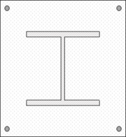
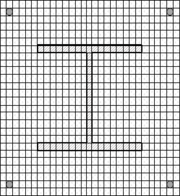
To make the analysis of the deformed cross-section condition and obtain the bearing capacity and its stiffness, a section discretization is made. In plane structures study, the layer discretization is satisfactory [23]. Herein, the residual stresses will be introduced explicitly in the steel cross-section. Thus, the two-dimensional discretization will be done, as shown in Figure 1.

The concept of sub-regions is then applied (Figure 1(b)). By means of a structured mesh generator, the cross-section is divided into smaller regions. Although only a full encased I-section is shown in Figure 1, the algorithm is applied to several types of steel, reinforced concrete and composite cross-sections.

(a) Cross section	(b) Definition of sub-regions	(c) Final discretization
Figure 1. Cross section discretization

As an initial parameter, the discretization has provided the number of divisions in both directions ($xy$) as input data. After obtaining the sub-regions, a search is made to find sections with larger areas. The main objective of this methodology is to generate a fiber mesh with approximately equal sizes throughout the cross-section minimizing errors in obtaining the section flexural stiffness.

After the discretization, some data are substantial to obtain the moment-curvature relation, through the Newton-Raphson method. They are the fiber areas and their respective positions. The $x$ and $y$ coordinates of each fiber are referenced to the section’s plastic centroid (PC), thereby minimizing convergence problems [30]. As defined by Chen et al. [31], as the origin of the reference system for the positions of the fiber areas, there is the possibility of using the geometric centroid of the section, or even the PC. The latter is better to avoid problems of non-convergence in asymmetric sections under bi-axial moments when subjected to high axial compression loads. Although in the present study symmetrical sections under uni-axial moments are approached, the reference axes in PC is used and it is defined as follows [32]:

$x_{pc}={\frac {x_{c}A_{c}f_{c}+x_{s}A_{s}f_{y}+x_{r}A_{r}f_{yr}}{A_{c}f_{c}+A_{s}f_{y}+A_{r}f_{yr}}}\qquad$ and $\qquad y_{pc}={\frac {y_{c}A_{c}f_{c}+y_{s}A_{s}f_{y}+y_{r}A_{r}f_{yr}}{A_{c}f_{c}+A_{s}f_{y}+A_{r}f_{yr}}}$

(1)

where $A_{c}$, $A_{s}$ and $A_{r}$ are the concrete, steel section and reinforcement areas; $x_{c}$, $x_{s}$ and $x_{r}$, $y_{c}$, $y_{s}$ and $y_{r}$ are the coordinates of the centroid, of the respective areas, relative to an initial reference system; and $f_{c}$, $f_{y}$ and $f_{yr}$ are the strengths of the concrete, steel section and reinforcement bars, respectively.

2.2. Residual stresses and materials constitutive models

Although the SCM-based methodology is generalized, that is, applicable to any cross-section type, this paper focuses exclusively on the steel and steel-concrete composite I-sections’ behavior submitted to 2D eccentric loads. Thus, the residual stress models used in this research are defined by design codes for this type of cross-section.

The EC3 [29] uses the residual stress model based on Huber and Beedle’s [3] proposition, shown in Figure 2(b). In this model, the stresses are arranged in the cross-section plates by a bilinear distribution. Furthermore, the $\sigma _{r}$ values depend directly on the relation between the cross-section height $h$ and its width $b$, as follows:

${\sigma }_{r}=\left\{{\begin{array}{c}0.5f_{y},{\mbox{ }}{\mbox{ }}{\mbox{ }}h/b\leq 1.2\\0.3f_{y},{\mbox{ }}{\mbox{ }}{\mbox{ }}h/b>1.2\end{array}}\right.$

(2)

where $f_{y}$ is the yield strength of the steel section, $b$ is the flange width and $h$ is the section height.

(a) Steel section	(b) EC3 [29]	(c) AISC [28]
Figure 2. Design codes models to describe the residual stresses

AISC [28] follows the proposal of Galambos and Ketter [4] that describes the residual stresses at the flanges in a similar way, but with different maximum values of tensile, ${\sigma }_{rt}$, and compression, ${\sigma }_{rc}$. In the web, the distribution is constant, as shown in Figure 2(c), and described as:

$\left\{{\begin{array}{c}{\sigma }_{rc}=0.3f_{y}\\{\sigma }_{rt}=\displaystyle {\frac {{\sigma }_{rc}bt}{bt+w(h-2t)}}\end{array}}\right.$

(3)

where $t$ and $w$ are the flange and web thickness, respectively.

2.3. Steel constitutive relationship

For both profile steel and reinforcement steel, the elastic-perfectly plastic constitutive model describes the material uniaxial behavior. The steel has isotropic behavior, i.e., the tensile and compression behavior is exactly the same. Thus, in Figure 3, only the section referring to the first quadrant of the constitutive relationship is shown.

Figure 3. Steel constitutive model

Since the behavior of the profile steel and the reinforcement bars is the same, just by changing the variables, the equation referring to only one of them (profile) will be presented. Thus, the steel constitutive relationship is written as follows:

${\sigma }_{s}=\left\{{\begin{array}{c}-f_{y},-{\epsilon }_{u}\leq \epsilon \leq -{\epsilon }_{y}\\E_{s}\epsilon ,-{\epsilon }_{y}<\epsilon <{\epsilon }_{y}\\f_{y},{\epsilon }_{y}\leq \epsilon \leq {\epsilon }_{u}\end{array}}\right.$

(4)

where $f_{y}$ is the yield steel strength, $\epsilon _{y}$ and ${\epsilon }_{u}$ are the yield and ultimate strains, respectively, and $E_{s}$ is the modulus of elasticity. The subindex $r$ may be added for the reinforcement variables.

2.4. Uniaxial behavior of concrete

Concrete has distinct mechanical properties with respect to tensile and compression. With respect to tensile, this material exhibits maximum strength $f_{cr}$ (Figure 4(b)). It is also emphasized that when the strength $f_{cr}$ is reached, the cracking process begins. The concrete loses strength and stiffness in case of strains greater than $\varepsilon _{cr}$. Thus, several researchers and even design codes disregard their contribution when tensioned. In the present study, under tensile, the constitutive relationship proposed by Vecchio and Collins [33], shown in Figure 4(b), is used. The compressed concrete is modeled as defined in Chiorean [18], as it is the second-degree parabola presented in a reduced form. Thus, to describe the concrete behavior we have:

$\sigma _{c}=\left\{{\begin{array}{lc}E_{tr}\varepsilon ,&0\leq \varepsilon \leq \varepsilon _{cr}\\f_{cr}\displaystyle {\frac {\alpha _{1}\alpha _{2}^{2}}{1+{\sqrt {500\varepsilon }}}}&\varepsilon >\varepsilon _{cr}\\-\left[\displaystyle {\frac {2\varepsilon }{\varepsilon _{ci}}}-\left(\displaystyle {\frac {\varepsilon }{\varepsilon _{ci}}}\right)^{2}\right]f_{c},&\varepsilon _{ci}\leq \varepsilon \leq 0\\-f_{c}\left[1-\gamma \left(\displaystyle {\frac {\varepsilon -\varepsilon _{ci}}{\varepsilon _{cu}}}-\varepsilon _{ci}\right)\right],&\varepsilon _{cu}\leq \varepsilon \leq \varepsilon _{ci}\end{array}}\right.$

(5)

in which $\varepsilon _{ci}$, $\varepsilon _{cu}$ and $\varepsilon _{cr}$ are the limit strain of the compressive non-linear behavior of concrete, the concrete ultimate strain in compression, and the initial cracking strain, respectively; $f_{cr}$ is the cracking strength of the concrete taken as 1.4 $(f_{c}/10)^{2/3}$ [32]; $E_{tr}$ is the concrete Young’s modulus in tensile before the cracking; $\alpha _{1}$ is the factor that considers the interaction of the reinforcement bars and the concrete, and $\alpha _{2}$ considers the effects of load duration and cyclic loads. Finally, $\gamma$ is the parameter associated with the concrete softening.

(a) Compression behavior	(b) Tensile behavior
Figure 4. Concrete constitutive relationship

2.5. Moment-curvature relationship

In this work, the Newton-Raphson iterative method is used to obtain the moment-curvature relationship ($M-\Phi$). For a fixed axial force value, $N$, increments are given at the external bending moment, $M$, until the full yield bending moment is reached. The incremental strategy is given by [34]:

$M_{j+1}=M_{j}+\Delta \Phi EI_{T}$

(6)

where $\Delta \Phi$ is a constant curvature increment given as input data and $EI_{T}$ is the tangent flexural stiffness, presented in Subsection 2.6.

Figure 5. Linear strains field around x axis

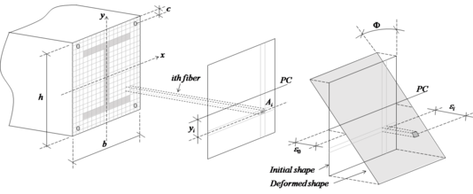
Figure 5 illustrates the linear distribution of strains in the steel cross-section under an axial force-bending moment combination. Note that the total axial strain at the $i$th fiber, $\varepsilon _{i}$, is given by a linear function. Therefore:

${\varepsilon }_{i}={\varepsilon }_{0}+{\varepsilon }_{ri}+\Phi y_{i}$

(7)

where $y_{i}$ is the distance between the plastic centroid (PC) of the analyzed fiber and the cross-section PC, ${\varepsilon }_{0}$ is the axial strain in the section PC, ${\varepsilon }_{ri}$ is the residual strain, and $\Phi$ its curvature. After discretization, the residual stresses $\sigma _{ri}$ are calculated in the center of each subarea, later these stresses are transformed into residual strains ($\varepsilon _{ri}$) via Hooke's law ($\varepsilon _{ri}=\sigma _{ri}/E_{s}$).

The variables ${\varepsilon }_{0}$ and $\Phi$ are the positions of the strain vector ${\boldsymbol {X}}=[{\varepsilon }_{0}\,\Phi ]^{T}$. It is necessary to adjust the vector ${\boldsymbol {X}}$ until the deformed shape of the section is consistent with the external forces. Numerically, it can be said the section equilibrium is obtained when the following equation is satisfied:

${\boldsymbol {F}}\left({\boldsymbol {X}}\right)={\boldsymbol {f}}_{ext}-$${\boldsymbol {f}}_{int}\cong {\boldsymbol {0}}$

(8)

where the external forces vector, ${\boldsymbol {f}}_{ext}$, is defined by the axial force, $N$, and bending moment, $M$.

However, the internal force vector is given by classical integral expressions for the axial force, $N_{int}$, and bending moment, $M_{int}$. Once areas, $A_{i}$, and positions, $y_{i}$, of each fiber are known, the integral becomes the sum described as:

${\boldsymbol {f}}_{int}=\left\{{\begin{array}{c}N_{int}=\int _{A}\sigma \left[\varepsilon ({\varepsilon }_{0},\Phi )\right]dA\\M_{int}=\int _{A}\sigma \left[\varepsilon ({\varepsilon }_{0},\Phi )\right]ydA\end{array}}\right\}\cong \left\{{\begin{array}{c}N_{int}\cong \sum _{i=1}^{n_{fib}}{\sigma }_{i}\left[{\varepsilon }_{i}({\varepsilon }_{0},\Phi )\right]A_{i}\\M_{int}\cong \sum _{i=1}^{n_{fib}}{\sigma }_{i}\left[{\varepsilon }_{i}({\varepsilon }_{0},\Phi )\right]{\mbox{ }}y_{i}A_{i}\end{array}}\right\}$

(9)

with $n_{fib}$ being the number of fibers used in the cross-section discretization. Fibers stresses, $\sigma _{i}$, are dependent on the deformed shape of the cross-section, and are therefore functions of ${\varepsilon }_{0}$.

While it is appropriate to initiate the process with ${\bf {X}}={\bf {0}}$, convergence is achieved in the first iteration only if external forces are null. Applying the expansion in Taylor series in Eq. (8), the results appear in the following set of non-linear equations:

${\boldsymbol {F}}({\boldsymbol {X}}+\delta {\boldsymbol {X}})=$${\boldsymbol {F}}({\boldsymbol {X}})+{\frac {\partial {\boldsymbol {F}}({\boldsymbol {X}})}{\partial {\boldsymbol {X}}}}\delta {\boldsymbol {X}}$

(10)

Starting from the supposed equilibrium at point ${\bf {X}}+\delta {\bf {X}}$, that is, ${\bf {F}}({\bf {X}}+\delta {\bf {X}})={\bf {0}}$, and knowing that $\delta {\bf {X}}={\bf {X}}^{k+1}-{\bf {X}}^{k}$, Eq. (10) can be rewritten as:

${\boldsymbol {X}}^{k+1}={\boldsymbol {X}}^{k}+{\boldsymbol {F}}{}'{\left({\boldsymbol {X}}^{k}\right)}^{-1}{\boldsymbol {F}}({\boldsymbol {X}}^{k})$

(11)

where ${\boldsymbol {F}}$ is the Jacobian matrix of the non-linear problem stated in Eq. (8). That is:

${\boldsymbol {F}}'=\left(-{\frac {\partial {\boldsymbol {F}}}{\partial {\boldsymbol {X}}}}\right)=\left[{\begin{array}{cc}f_{11}=\displaystyle {\frac {\partial N_{int}}{\partial {\varepsilon }_{0}}}&f_{12}=\displaystyle {\frac {\partial N_{int}}{\partial \Phi }}\\f_{21}=\displaystyle {\frac {\partial M_{int}}{\partial {\varepsilon }_{0}}}&f_{22}=\displaystyle {\frac {\partial M_{int}}{\partial \Phi }}\end{array}}\right]$

(12)

The term $f_{11}$ can be determined as follows:

$f_{11}={\frac {\partial N_{int}}{\partial {\varepsilon }_{0}}}=$${\frac {\partial }{\partial {\varepsilon }_{0}}}\left[\int _{A}\sigma \left[\varepsilon ({\varepsilon }_{0},\Phi )\right]dA\right]=$${\frac {\partial }{\partial {\varepsilon }_{0}}}\left[\int _{A}\sigma ({\varepsilon }_{0}+\right.$$\left.{\varepsilon }_{ri}+\Phi y_{i})dA\right]$

(13)

in which it becomes necessary to use the Chain Rule to solve the previous equation. That is:

$f_{11}=\int _{A}\left({\frac {\partial \sigma }{\partial \varepsilon }}{\frac {\partial \varepsilon }{\partial {\varepsilon }_{0}}}\right)dA=$$\int _{A}\left({\frac {\partial \sigma }{\partial \varepsilon }}{\frac {\partial ({\varepsilon }_{0}+{\varepsilon }_{ri}+\Phi y_{i})}{\partial {\varepsilon }_{0}}}\right)dA=$$\int _{A}{\frac {\partial \sigma }{\partial \varepsilon }}dA$

(14)

The derivative of stress, $\sigma$, with respect to strain, $\varepsilon$, results in the tangent modulus of elasticity, $E_{T}$. In this way, $f_{11}$ can be write as:

$f_{11}=\int _{A}E_{T}dA=\sum _{i=1}^{n_{fib}}E_{T,i}A_{i}$

(15)

Analogous to the development of $f_{11}$, the other terms of ${\boldsymbol {F}}'$ are given by:

$f_{12}={\frac {\partial N_{int}}{\partial \Phi }}={\frac {\partial }{\partial \Phi }}\left[\int _{A}\sigma \left[\varepsilon ({\varepsilon }_{0},\Phi )\right]dA\right]=$$\int _{A}E_{T}ydA=\sum _{i=1}^{n_{fib}}E_{T,i}y_{i}A_{{\mbox{ }}i}$

(16)

$f_{21}={\frac {\partial M_{int}}{\partial {\varepsilon }_{0}}}=$${\frac {\partial }{\partial {\varepsilon }_{0}}}\left[\int _{A}\sigma \left[\varepsilon ({\varepsilon }_{0},\Phi )\right]ydA\right]=$$\int _{A}E_{T}ydA=\sum _{i=1}^{n_{fib}}E_{T,i}y_{i}A_{i}$

(17)

$f_{22}={\frac {\partial M_{int}}{\partial \Phi }}={\frac {\partial }{\partial \Phi }}\left[\int _{A}\sigma \left[\varepsilon ({\varepsilon }_{0},\Phi )\right]ydA\right]=$$\int _{A}E_{T}y^{2}dA=\sum _{i=1}^{n_{fib}}E_{T,i}y_{i}^{2}A_{i}$

(18)

The convergence criterion adopted in this paper is based on the ratio of the Euclidean norms of the unbalanced force vector, ${\bf {F}}$, and the external forces vector, ${\bf {f}}_{ext}$. Thus, this ratio should be less than a tolerance, which is assumed to be 10^-5 here.

2.6. Flexural stiffness

The analysis of the cross section starts with the plastic centroid (PC) fixed in the position given by Eq. (1). However, as the internal forces vary, the deformed configuration of the section starts to present increasingly larger axial strains and, consequently, the PC changes position. In this way, the PC position is evaluated as:

$y_{PC}={\frac {\displaystyle \int _{A}E_{T}ydA}{\displaystyle \int _{A}E_{T}dA}}=\displaystyle {\frac {\displaystyle \sum _{i=1}^{n_{fib}}E_{T,i}y_{i}A_{i}}{\displaystyle \sum _{i=1}^{n_{fib}}E_{T,i}A_{i}}}$

(19)

Tangent flexural stiffness, that is, using values of the modulus of elasticity tangent to the constitutive relationships, must be calculated in relation to the updated position of the PC, $y_{PC}$. Thus, the $EI_{T}$ stiffness is given by:

$EI_{T}=\int _{A}{\left(y-y_{PC}\right)}^{2}E_{T}dA=\int _{A}y^{2}E_{T}dA-$$\int _{A}2(y)(y_{PC})E_{T}dA+\int _{A}y_{PC}^{2}E_{T}dA$

(20)

Since the system is discretized in fibers, the integrals of the previous equation become summations. That is:

$EI_{T}=\sum _{i=1}^{n_{fib}}y_{i}^{2}E_{T,i}A_{i}-2\sum _{i=1}^{n_{fib}}y_{i}E_{T,i}A_{i}y_{CP}+\sum _{i=1}^{n_{fib}}E_{T,i}A_{{\mbox{ }}i}y_{CP}^{2}$

(21)

Substituting the value of $y_{PC}$ (Eq. (19)) in Eq. (21), we arrive at:

$EI_{T}=\displaystyle \sum _{i=1}^{n_{fib}}y_{i}^{2}E_{T,i}A_{i}-2\displaystyle \sum _{i=1}^{n_{fib}}y_{i}E_{T,i}A_{i}\left({\frac {\displaystyle \sum _{i=1}^{n_{fib}}E_{T,i}y_{i}A_{i}}{\displaystyle \sum _{i=1}^{n_{fib}}E_{T,i}A_{i}}}\right)+{\displaystyle \sum _{i=1}^{n_{fib}}E_{T,i}A_{i}\left({\frac {\displaystyle \sum _{i=1}^{n_{fib}}E_{T,i}y_{i}A_{i}}{\displaystyle \sum _{i=1}^{n_{fib}}E_{T,i}A_{i}}}\right)}^{2}$

(22)

which can be reduced to:

$EI_{T}=\displaystyle \sum _{i=1}^{n_{fib}}y_{i}^{2}E_{T,i}A_{i}-\displaystyle \sum _{i=1}^{n_{fib}}y_{i}E_{T,i}A_{i}{\frac {\displaystyle \sum _{i=1}^{n_{fib}}E_{T,i}y_{i}A_{i}}{\displaystyle \sum _{i=1}^{n_{fib}}E_{T,i}A_{i}}}$

(23)

Correlating Eqs. (15-18) to Eq. (23), it is noted that $EI_{T}$ can be described in terms of the constitutive matrix of the cross section. Thus, the flexural stiffness of the section can be written as:

$EI_{T}=f_{22}-{\frac {f_{12}f_{21}}{f_{11}}}$

(24)

Graphically, the previous equation refers to the tangent flexural stiffness to the moment-curvature relationship.

2.7. Yield curves

When, for a given axial force, the maximum bending moment of the moment-curvature is reached, there is a total section plastification. It is defined such that a pair of forces is a point on the full yield curve. Thus, the procedure described in Subsection 2.3 is made for each increment of the bending moment until it singularizes the Jacobian matrix or a fiber reaches the maximum axial strain of its component material, defined by the constitutive relationship. The bending moments used for the full yield curve are defined considering the limit point of the moment-curvature relationship (maximum bending moment), since after this point is reached, the cross-sectional softening process begins. Considering the applicability of these curves obtained here in the RPHM and a numerical methodology that neglects this effect, the descending stretches of the moment-curvature relationship [35,36] will be neglected in this approach.

The initial yield curve is also obtained from the moment-curvature relationship. When the first fiber of the section presents an axial strain, $\varepsilon _{i}$, greater than the yield strain of the steel, $\varepsilon _{y}$, and/or the initial yield strain of the concrete, $\varepsilon _{ci}/2$ [21], the fiber begins to degrade, causing the section to consequently lose stiffness. The moment responsible for this fact is considered the initial yield bending moment.

The flowchart for obtaining the interaction curves is illustrated in Figure 6.

Figure 6. Flowchart for obtaining the interaction curves

3. Numerical applications

In this section, the numerical procedure described in this paper will be applied. Isolated steel I-sections and an encased steel I-section will be studied. In both cases, the modeling calibration is initially carried out considering the results present in the literature. Thus, moment-curvature and bending moment-flexural stiffness relationships are plotted to assess the accuracy of the approach described in this paper. In a second step, the interaction curves are presented and discussed. In all the data simulated here, a constant increment of curvature, $\Delta \Phi$ (Eq. (6)), equal to 0.001/m was used.

3.1. Steel sections

Zubydan [26] analyzed the flexural stiffness variation in I (UB) and H (UC) sections versus the increase of the bending moment acting in the cross-section. The author exclusively studied steel elements under minor axis bending. Thus, the author used the considerations of EC3 [29] to define the residual stresses distribution. The material yield strength is 25 kN/cm² and Young’s modulus is given by 20000 kN/cm².

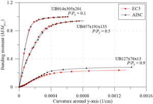
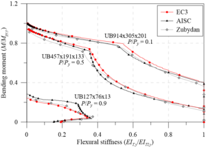
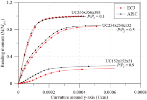
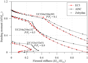
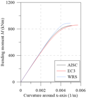
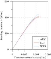
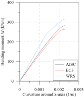
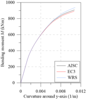
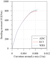
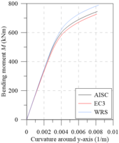
Figure 7 shows the moment-curvature and bending moment-flexural stiffness curves for both UC and UB sections using the EC3 [29] and AISC [28] considerations. Through Figures 7(b) and 7(d), the good agreement between the results obtained considering the European residual stress model with the Zubydan [26] results, for both UB and UC sections is shown. Using the AISC [28] model, a good proximity to the other results for the UB sections can be observed. These cross-sections have a height that is greater than the width; thus, the residual compressive stress at the flange ends is equivalent to the EC3 [29] residual stresses, which considerably approximate the responses (Figure 7(c)).

(a) UB sections: Moment-curvature relationship	(b) UB sections: Bending moment-flexural stiffness
(c) UC sections: Moment-curvature relationship	(d) UC sections: Bending moment-flexural stiffness
Figure 7. Steel UB and UC non-linear behavior

Using the normative approaches described in item 2.2, Figure 7(d) does not show the same convergence between the results. It was verified that in all the analyzed cases, the sections with the American residual stress model began to lose flexural stiffness for larger values of bending moment than the simulations with the EC3 model [29]. This situation occurs because in UC sections, the EC3 [29] prescription defines the value of $\sigma _{r}$ as 0.5 $f_{y}$; and in AISC [28], the same values that are assigned to I-sections are used in this case, i.e., $\sigma _{rc}=0.3f_{y}$. As the tensile stresses are always smaller than the compression stresses, it can be stated that the AISC [28] presents a greater domain for the elastic range of the cross-section.

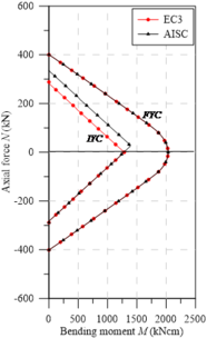
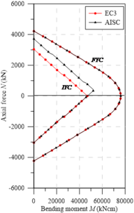
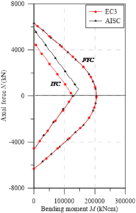
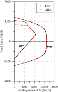
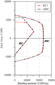
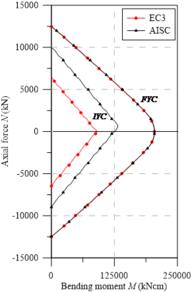
To validate the assertion made above, the IYCs and FYCs are shown in Figures 8-11. It is verified that the approaches already present in literature [20] are equivalent to the IYCs obtained using the EC3 [29] residual stress model in elements under major axis bending.

When verifying the IYCs considering the AISC [28] model, an asymmetry in the horizontal axis can be observed. This fact is determined by the constant distribution of residual tensile stresses in the section web. The values of $\sigma _{rt}$ when under normal tensile force and the value of $\sigma _{rc}$ when under compression are determinant in obtaining the IYC; this fact contributes to a greater elastic region in the $NM$ diagrams.

(a) UB $127\times 76\times 13$	(b) UB $457\times 191\times 133$	(c) UB $914\times 305\times 201$
Figure 8. Yield curves for UB sections - major axis bending

(a) UB $127\times 76\times 13$	(b) UB $457\times 191\times 133$	(c) UB $914\times 305\times 201$
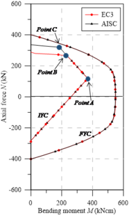
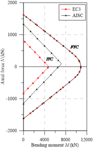
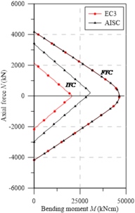
Figure 9. Yield curves for UB sections - minor axis bending

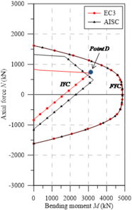
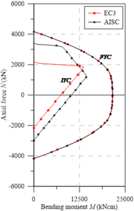
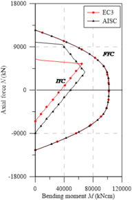
However, when analyzing the IYCs in the minor axis, the asymmetry on the horizontal axis is more pronounced. A divergence in the curves’ behavior obtained for the major and minor axes is then observed. It has been found that the behavior shown in the curves arises from the models presenting their higher tensile stresses in the web and in the flange center, on the section plastic centroid. Thus, under compression loads, the behavior is perfectly linear with a greater influence of the bending moment. Under tensile stresses, however, the axial load becomes more relevant, completely changing the curve shape.

(a) UB $127\times 76\times 13$	(b) UB $457\times 191\times 133$	(c) UB $914\times 305\times 201$
Figure 10. Yield curves for UC sections - major axis bending

(a) UB $127\times 76\times 13$	(b) UB $457\times 191\times 133$	(c) UB $914\times 305\times 201$
Figure 11. Yield curves for UC sections - minor axis bending

Three points are highlighted in Figure 9(a): $A$, $B$ and $C$. Point $A$ represents the situation where the cross section shows the greatest bending moment within the elastic regime. For the UB sections, it is apparent that this point is coincident for both residual stress models, EC3 [29] and AISC [28]. This is because both these models present compression stresses at the flanges ends equal to 0.3$f_{y}$. For minor axis bending, these stresses are responsible for determining the maximum possible elastic bending moment in the section. To reach this moment, an axial tensile force, $N_{a}$, capable of canceling the value of the residual compression stresses (0.3$f_{y}$) is required, that is:

$N_{a}=A_{g}\left(0.3f_{y}\right)$

(25)

where $A_{g}$ is the steel section area and $f_{y}$ is the material yield strength.

Thus, the maximum tensile stresses in the elastic bending are null before the bending moment application, so that it is given at point $A$ by:

$M_{a}=W_{y}f_{y}$

(26)

in which $W_{y}$ is the section elastic modulus in minor axis.

Points $B$ and $C$ differ by the maximum residual tensile stress values given in the design codes discussed in the present study. Eq. (2) defines the residual tensile stress in the middle of the flanges and the web given by EC3 [29] for UC sections as 0.3$f_{y}$, which is same value that is adopted for the compressed parts of the cross-section.

Note that residual tensile stresses occur on the PC, that is, they only influence the axial load, $N$. Thus, at point $B$, a horizontal plateau is evident, indicating that the tensions generated by the axial load at that point, together with the residual stresses (0.3$f_{y}$), are practically equal to $f_{y}$. That is, $N_{b}=A_{g}0.7f_{y}$. In relation to the bending moment, it should be noted that the normal stresses generated by $N_{b}$ are tensile, relieving residual compression stresses (-0.3$f_{y}$) at the webs ends. Thus, $M_{b}$ can be defined as $M_{b}=W_{y}$ (0.6$f_{y}$).

The AISC [28] defines $\sigma _{rt}$ as a function of the residual compressive stress, $\sigma _{rc}$. In Eq. (3), it is shown intuitively that in all cases, $\sigma _{rt}$ is less than $\sigma _{rc}$.

It can be stated that for this norm, the elastic regime is higher than in EC3 [29], as seen in Figure 9. Point $C$ is analyzed in the same manner as point $B$, except for using American code considerations.

Point $D$, as shown in Figure 11(a), follows the same approach shown in the UB sections curves. Note that the UC sections squarer in shape, modifying the value of $\sigma _{r}$ given by the European design code. In this situation, $\sigma _{r}=0.5f_{y}$. Thus, since the axial tensile force responsible for overriding the residual compressive stresses at the webs’ ends is $N_{d}=A_{g}(0.5f_{y}$), the maximum bending moment is obtained as described for point $A$, discussed above. However, by canceling these compressive stresses, the tensile stresses in the PC increase, which then reach the $f_{y}$ value. This description is very clear in Figure 11, where the EC3 [29] residual stress model is used.

With the present study, the need to review the initial yield curves for steel I-sections subjected to minor axis bending is evidenced. With a brief description of the ordered pairs referring to points $A$, $B$, $C$ and $D$, it is possible to draw simplified curves, where the non-linear procedure located in the cross-section can be avoided by reducing the processing time in the numerical structural analyses via RPHM. It is worth mentioning in the study by Gonçalves et al. [37], for the application of the RPHM for the analysis of elements under minor-axis bending, the authors had to use the tangent elastic modulus for the flexural stiffness degradation, since the initial yield curves did not portray the reality.

3.2. Steel-concrete composite section

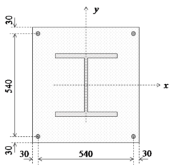
Chiorean [18] presented a study of the influence of residual stress models on the steel-concrete composite section behavior as shown in Figure 12. This is a W12$\times$120 section that is fully encased in concrete and reinforced by 4 20 mm diameter bars. The section dimensions $h$, $b$ and $c$, defined in Figure 3, are taken as 600 mm, 60 0mm and 30 mm, respectively. The strengths steel section, reinforcement steel and compressive concrete strengths are taken equal to 30, 40 and 2 kN/cm², respectively. The modulus of elasticity of the steel section and the reinforcement are equal to 20000 kN/cm². In addition, it is noted that the concrete limit strains, in concrete, the final strain of the second-degree parabola, $\varepsilon _{ci}$, was taken as 0.002 and the ultimate strain was defined as 0.0035. The steel ultimate strain was taken as 0.01. The concrete softening was simulated by the parameter $\gamma =0.15$, and was considered $\alpha _{1}=1$ and $\alpha _{2}=0.75$ for the concrete tensile behavior [18].

Figure 12. W12$\times$120 section totally encased in concrete (dimensions in mm)

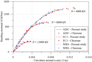
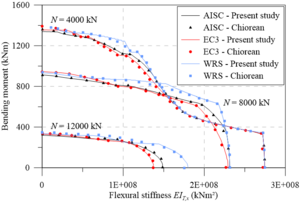
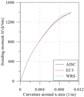
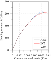
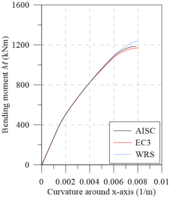
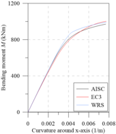
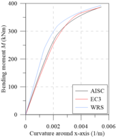
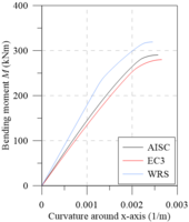
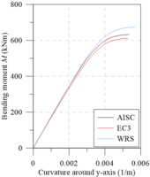
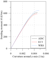
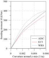
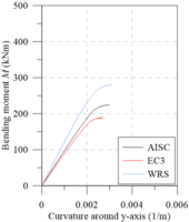
Chiorean [18] performed several analyses using both EC3 [29] and AISC [28] residual stress models. Additionally, results were also generated disregarding the effect of such residual stresses (WRS data). All these analyses were also done in the present work in order to calibrate the models, and to verify the initial (IYCs) and full (FYCs) yield curves of this composite section. Another aim of this analysis is the evaluation of the influence of the elastic limit strain of the concrete elastic regime ($\varepsilon _{ci}/2$) [21] on definitions of IYCs. The moment-curvature relationship (Figure 13(a)) and flexural stiffness-bending moment curves (Figure 13(b)) for the major axis are presented below. The results in all cases were compared with literature. For each curve, the axial force values were set as: 4000 kN, 8000 kN and 12000 kN. The numerical procedure described in item 2.5 was, thus, used.

(a) Moment-curvature relationship – major axis	(b) Moment-flexural stiffness – major axis
(c) Moment-curvature relationship – minor axis	(d) Moment-flexural stiffness – minor axis
Figure 13. Analysis of steel-concrete composite section

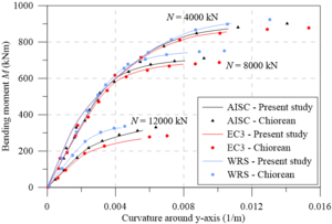
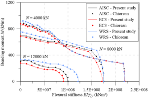
Results of the analyses were observed to be in good agreement with the results obtained by Chiorean [18]. It is worth mentioning that in some cases, the moment-curvature relationships found in the present study are less ductile than those in the literature. Although procedures used are similar, the stopping criteria are different as they directly influence the moment-curvature relationship’s critical bending moment.

All the curves in Figure 13(b) demonstrate a marked decrease in flexural stiffness. This decrease is related to the cracking start in the most tensioned fibers and the consequent decrease of the concrete tangent modulus of elasticity. Note that in the literature for approaches to steel-concrete composite structures [21,23,24], this fact is considered in a simplified form, for example, the 40% reduction in concrete section flexural stiffness. Thus, to eliminate the approximation, there should be three curves within the NM diagram, i.e., in addition to the FYC and IYC, there is a need for an initial cracking curve for a more realistic simulation [22].

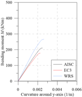
The comparison of the moment-curvature relationships (Figure 13(a)) and the bending moment-flexural stiffness curves (Figure 13(b)) shows a slight divergence in the EC3 [29] and AISC [28] responses. In these figures, it is clear how the AISC [28] approach allows for greater stiffness than the EC3 [29] approach. This is because the W12$\times$120 section is almost shaped like a square, that is, $h/b<1.2$. Thus, the European code defines that the maximum residual stresses acting in the section reach 0.5$f_{y}$, which differs from Galambos and Ketter’s [4] proposal.

It is also worth mentioning that, in the analysis without residual stresses (WRS results), it is observed, as expected, a more rigid behavior for all the moment-curvature relationships as well as presented in bending moment-flexural stiffness curves.

The same observations made for analysis around the major axis can now be made for the minor axis (Figures 13(c) and 13d), which, although when presenting curves with different values, the observed behavior is quite similar.

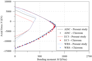
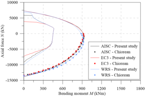
Figures 14(a) and 14(b) show both IYCs and FYCs obtained using the EC3 [29] and AISC [28] requirements for the major and minor axes bending. In addition, the results found disregarding residual stresses are also presented. It is worth mentioning that there was good accuracy between the results obtained in the present study and those presented by Chiorean [18]. Although practically equal procedures have been used to obtain the moment-curvature relationship, the stopping criterion is different. This criterion is precisely the one responsible for defining the FYCs points, which validates the use of the Jacobian matrix singularity in the definition of the cross-section-bearing capacity. As can be observed in Figures 14(a) and 14(b), there is a slight difference in the FYCs using the residual stresses of EC3 [29] and AISC [28]. The main factor of comparison is in the IYCs. There is a significant divergence for the major and minor axes, and in both situations, the AISC [28] model provided a higher elastic region within the $NM$ diagrams. It is also noted that when neglecting the effect of residual stresses, the elastic region of the $NM$ diagram is amplified, as expected. Furthermore, it can be verified for intermediate values of $N$, the IYCs are coincident for the three results, defining that for these values, the strain $\varepsilon _{ci}$ is responsible for defining the referred curve.

(a) IYC and FYC – Major axis	(b) IYC and FYC – Minor axis
Figure 14. Yield curves of composite section

Additionally, a study was carried out considering the variation of the parameter $\gamma$, which deals with the concrete softening under compression. In Figures 15 and 16, major and minor axes bending, respectively, are presented moment-curvature relationships considering axial compressive forces of 4000 kN, 8000 kN and 12000 kN. In addition, the parameter $\gamma$ was adopted as 0, 0.5 and 1.

(a) For N = 4000 kN and $\gamma =0$	(b) For N = 4000 kN and $\gamma =0.5$	(c) For N = 4000 kN and $\gamma =1$
(d) For N = 8000 kN and $\gamma =0$	(e) For N = 8000 kN and $\gamma =0.5$	(f) For N = 8000 kN and $\gamma =1$
(g) For N = 12000 kN and $\gamma =0$	(h) For N = 12000 kN and $\gamma =0.5$	(i) For N = 12000 kN and $\gamma =1$
Figure 15. Influence of concrete softening parameter $\gamma$ in major axis bending

It can be seen for both major and minor axes bending, for the axial compressive force of 4000 kN, the flexural stiffness is largely similar to the moment-curvature relationship, considering the residual stress models of AISC [28], EC3 [29] and still despising them (WRS). Graphically, you can see a slight difference in the maximum bending moment for these cases. See also that although the bearing capacity decreases as $\gamma$ increases, the consideration or not of the residual stresses in the analysis has little influence on the final response of the cross-sectional behavior.

As for the force of 12000 kN, it can be seen that this proximity in the flexural stiffness of the three curves means that the initial stiffness of the moment-curvature relationship is not the same. The effect of residual stresses is more noticeable than in the analyzes considering axial compressive forces of 4000 kN and 8000 kN. Furthermore, even for the force of 12000 kN, the greatest differences between the maximum bending moments are found. Furthermore, when considering the EC3 [29] residual stress model, it can be seen that it implies a reduction in the bearing capacity. In addition, disregarding residual stresses promotes analyzes with higher strength capacities in all cases.

(a) For N = 4000 kN and $\gamma =0$	(b) For N = 4000 kN and $\gamma =0.5$	(c) For N = 4000 kN and $\gamma =1$
(d) For N = 8000 kN and $\gamma =0$	(e) For N = 8000 kN and $\gamma =0.5$	(f) For N = 8000 kN and $\gamma =1$
(g) For N = 12000 kN and $\gamma =0$	(h) For N = 12000 kN and $\gamma =0.5$	(i) For N = 12000 kN and $\gamma =1$
Figure 16. Influence of concrete softening parameter $\gamma$ in minor axis bending

The force of 8000 kN generated intermediate data in relation to those mentioned above. Thus, it can be concluded the residual stresses are more pronounced as the axial compressive force increases, and at the same time that the concrete softening effect is considered with greater intensity.

4. Conclusions

The present study evaluated the behavior of steel I-sections considering two residual stress models prescribed in design codes [28,29]. For the analyses, a SCM-based non-linear methodology was used, where the constitutive relationships and the residual stresses were explicitly used.

The curves that were obtained and plotted focused on the two methodologies of plasticity simulation in the refined plastic hinge method (RPHM): the use of the moment-curvature relationship and the initial (IYC) and full (FYC) yield curves. In the first step, the numerical approach was calibrated with comparisons of the results found in the present work along with data provided in the literature [18,26]. In a second step, the yield curves for bare steel sections and for a steel concrete-composite section were generated.

Some general conclusions can be made. They are as follows:

• In the calibration of the results, it was possible to verify the formulation accuracy in relation to the reference data for both bare steel and steel-concrete composite tested sections;
• In general, regardless of the adopted residual stresses model, the FYCs were practically identical for the bare steel sections, and very similar for the composite section. Thus, it can be concluded that the adopted residual stresses model does not change the bearing capacity of the cross-sections;
• For the bare steel section, the IYCs in the minor axis bending analysis presented asymmetry in relation to the horizontal axis (bending moment). This asymmetry demonstrates the need to review the propositions of the RPHM for the evaluation of minor axis bending;
• The IYCs can be defined through specific analytically calculated points. In the present work, they were defined as points $A$, $B$, $C$ and $D$;
• In all simulated cases, the AISC [28] approach defines a larger elastic region within the NM diagrams. A more detailed study of the UB $914\times 305\times 201$ section provided a range of quantitative parameters for the validation of the above information. By comparing all the bending moment increments in the moment-curvature analysis, it was found that, on average, the analysis using the European residual stress model was 4.81% less rigid than the one using the American model;
• Still observing the IYC of UB $914\times 305\times 201$, we can see that the differences between the design code models appear for the tensiled section. In this case, for example, the average difference between the bending moments is 31.25% for the major axis bending. This cross section was chosen because the graphical responses of the moment-curvature relationships using the two residual stress models was very closed;
• For the analysis of the steel-concrete composite section, it was noticeable the effects of residual stresses become more relevant as the axial compressive forces increase and the softening effect of the concrete is treated with greater intensity.

Author’s Contribuitions

Ígor JM Lemes: Conceptualization, Methodology, Software, Validation, Writing – original draft, Data curation. Jéssica L. Silva: Methodology, Data curation, Writing – original draft. Everton AP Batelo: Methodology, Data curation, Writing – original draft. Ricardo AM Silveira: Methodology, Writing – review & editing, Funding acquisition, Supervision.

Acknowledgments

The authors acknowledge the financial support of the Brazilian research agencies CNPq [grant number 307898/2019-9], CAPES, FAPEMIG [grant number TEC-PPM-00221-18], and PROPPI/UFOP, UFLA and UFMT for their support during the preparation of this work.

Conflicts of interest: none.

References

[1] Grilo L.F., Fakury R.H., Silva A.L.R.C., Rodrigues F.C., Daldegan V.P. Behavior and design of built-up compressed steel members composed of concentric hot rolled circular hollow sections. Lat. Am. J. Solids Struct., 15(6):e51, 2018 https://doi.org/10.1590/1679-78254570

[2] Alvarenga A.R. The semi-rigid connections in the plastic zone advanced analysis of steel plane frames. D. Sc. Thesis (in Portuguese), Federal University of Ouro Preto, Brazil, 2010.

[3] Huber A.W.E., Beedle L.S. Residual stress and the compressive strength of steel. Weld J., 33:589–614, Reprint No. 96:54-3, 1954.

[4] Galambos T.V., Ketter R.L. Columns under combined bending and thrust. J. Eng. Mech. Div-ASCE, 85:1-30, 1959. https://doi.org/10.1061/TACEAT.0008059

[5] Abambres M., Quach W.-M. Residual stresses in steel members: a review of available analytical expressions. Int. J. Struct. Integr., 7(1):70-94, 2016. https://doi.org/10.1108/IJSI-12-2014-0070

[6] Clarin M. High strength steel: local buckling and residual stresses. Licentiate Thesis 2004:54, Lulea University of Technology, Lulea. 2004.

[7] Fukumoto Y., Itoh Y. Statistical study of experiments on welded beams. J. Struct. Div-ASCE, 107(1):89-103, 1981. https://doi.org/10.1061/JSDEAG.0005639

[8] Young B.W. Residual stresses in hot-rolled sections. Proceedings of the IABSE International Colloquium on Column Strength, 23:25-38, 1975.

[9] Hadjioannou M., Douthe C., Gantes C.J. Influence of cold bending on the resistance of wide flange members. Int. J. Steel Struct., 13(2):353-366, 2013. https://doi.org/10.1007/s13296-013-2013-6

[10] Weng C.C., Pekoz T. Residual stresses in cold-formed steel members. J. Struct. Eng-ASCE, 116(6):1611-1625, 1990. https://doi.org/10.1061/(ASCE)0733-9445(1990)116:6(1611)

[11] Quach W.M., Teng J.G., Chung K.F. Finite element predictions of residual stresses in press-braked thin-walled steel sections. Eng. Struct., 28(5):1609-1619, 2006. https://doi.org/10.1016/j.engstruct.2006.02.013

[12] Liu W., Rasmussen K.J.R., Zhang H. Modelling and probabilistic study of the residual stress of cold-formed hol-low steel sections. Eng. Struct., 150:986-995, 2017. https://doi.org/10.1016/j.engstruct.2017.08.004

[13] Yao Y., Quach W.-M., Young B. Finite element-based method for residual stresses and plastic strains in cold-formed steel hollow sections. Eng. Struct., 188:24-42, 2019. https://doi.org/10.1016/j.engstruct.2019.03.010

[14] Tankova T., Silva L.S., Balakrishnam M., Rodrigues D., Launert B., Pasternak H., Tun T.Y. Residual stresses in welded I section steel members. Eng. Struct., 197:109398, 2019. https://doi.org/10.1016/j.engstruct.2019.109398

[15] Liu Y., Tsang K.S., Subramaniam N.A., Pang J.H.L. Structural fatigue investigation of thermite welded rail joints considering weld-induced residual stress and stress relaxation by cyclic load. Eng. Struct., 235:112033, 2021. https://doi.org/10.1016/j.engstruct.2021.112033

[16] Rossi A., Souza A.S.C, Nicoletti R.S., Martins C.H. The influence of structural and geometric imperfections on the LDB strength of steel–concrete composite beams. Thin-Walled Struct., 162:107542, 2021. https://doi.org/10.1016/j.tws.2021.107542

[17] Tremarin R.C., Chamberlain Z.M. Analysis of the influence of residual stress on fatigue life of welded joints. Lat. Am. J. Solids Struct., 17(3):e262, 2020 https://doi.org/10.1590/1679-78256020

[18] Chiorean C.G. A computer method for nonlinear inelastic analysis of 3D composite steel-concrete frame structures. Eng. Struct., 57:125–152, 2013. https://doi.org/10.1016/j.engstruct.2013.09.025

[19] Silva J.L., Deus L.R.R.M., Lemes Í.J.M, Silveira R.A.M. Plastic analysis of steel arches and framed structures with various cross sections. Steel Compos. Struct., 38(3):257-270, 2021. https://doi.org/10.12989/scs.2021.38.3.257

[20] Chan S.L., Chui P.P.T. Non-linear static and cyclic analysis of steel frames with semi-rigid connections. Elsevier Science (Oxford), 2000.

[21] Fong M., Chan S.L. Advanced analysis of steel-concrete composite beam-columns by refined plastic-hinge method. Int. J. Struct. Stab. Dy., 12(6):1250046, 2012. https://doi.org/10.1142/S0219455412500460

[22] Lemes Í.J.M., Barros R.C., Silveira R.A.M, Silva A.R.D., Rocha P.A.S. Numerical analysis of RC plane structures: a concentrated nonlinear effect approach. Lat. Am. J. Solids Struct., 15(2):e20, 2018. https://doi.org/10.1590/1679-78254681

[23] Lemes Í.J.M., Silveira R.A.M., Silva A.R.D., Rocha P.A.S. Nonlinear analysis of two-dimensional steel, reinforced concrete and composite steel-concrete structures via coupling SCM/RPHM. Eng. Struct., 147:12–26, 2017. https://doi.org/10.1016/j.engstruct.2017.05.042

[24] Lemes Í.J.M., Silva A.R.D., Silveira R.A.M, Rocha P.A.S. Numerical analysis of nonlinear behavior of steel-concrete composite structures. Rev. IBRACON Estrut. Mater., 10(1):53-83, 2017. https://doi.org/10.1590/S1983-41952017000100004

[25] Li T.J., Liu S.W., Chan S.L. Direct analysis for high-strength steel frames with explicit-model of residual stresses. Eng. Struct., 100:342-355, 2015. https://doi.org/10.1016/j.engstruct.2015.06.008

[26] Zubydan A.H. Inelastic second order analysis of steel frame elements flexed about minor axis. Eng. Struct., 33:1240–1250, 2011. https://doi.org/10.1016/j.engstruct.2010.12.046

[27] Deus L.R.R.M., Silveira R.A.M, Lemes Í.J.M., Silva J.L. Second-order inelastic analysis of shallow and non-shallow steel arches. Lat. Am. J. Solids Struct., 17(3):e265, 2020. https://doi.org/10.1590/1679-78255941

[28] AISC. Load and resistance factor design specification for structural steel buildings. American Institute of Steel Construction, Chicago, Illinois, USA, 2016.

[29] CEN (European Committee for Standardization). Design of steel structures: Part 1-1: General rules and rules for buildings. Eurocode 3, EN 1993-1-1, Brussels, Belgium, 2005.

[30] Barros R.C., Pires D., Silveira R.A.M., Lemes Í.J.M., Rocha P.A.S. Advanced inelastic analysis of steel structures at elevated temperatures by SCM/RPHM coupling. J. Construct. Steel Res., 145:368-385, 2020. https://doi.org/10.1016/j.jcsr.2018.03.001

[31] Chen S.F., Teng J.G., Chan S.L. Design of biaxially loaded short composite columns of arbitrary section. J. Struct. Eng., 127(6):678-685, 2001. https://doi.org/10.1061/(ASCE)0733-9445(2001)127:6(678)

[32] Lemes Í.J.M., Dias L.E.S, Silveira R.A.M., Silva A.R., Carvalho T.A. Numerical analysis of steel–concrete composite beams with partial interaction: A plastic-hinge approach. Eng. Struct., 248:113256, 2021. https://doi.org/10.1016/j.engstruct.2021.113256

[33] Vecchio F.J., Collins M.P. Modified compression-field theory for reinforced concrete elements subjected to shear. ACI J., 83(2):219–231, 1986. https://doi.org/10.14359/10416

[34] Lemes Í.J.M., Silva A.R.D, Silveira R.A.M, Rocha P.A.S. Determinação da capacidade resistente de elementos estruturais mistos através do método da rótula plástica refinado. Rev. Int. Métodos Numér. Cálc. Diseño Ing., 33(1-2):24-34 (in Portuguese), 2017. https://doi.org/10.1016/j.rimni.2015.10.003

[35] Chiorean C.G. Computerised interaction diagrams and moment capacity contours for composite steel–concrete cross-sections. Eng. Struct., 32(11):3734-3757, 2010. https://doi.org/10.1016/j.engstruct.2010.08.019

[36] Chiorean C.G. A computer method for moment-curvature analysis of composite steel-concrete cross-sections of arbitrary shape. Eng. Struct. Technol., 9(1):25-40, 2017. https://doi.org/10.3846/2029882X.2017.1299969

[37] Gonçalves G.A., Silva A.R.D., Silveira R.A.M. Avaliação do comportamento inelástico de colunas e pórticos metálicos com flexão em torno do eixo de menor inércia. Rev. Int. Métodos Numér. Cálc. Diseño Ing., 32(1):13-21, 2016. https://doi.org/10.1016/j.rimni.2014.07.002