Parameter estimation in ODEs. Modelling and computational issues

Parameter estimation in ODEs. Modelling and computational issues

Abstract. In this work we discuss a variational approach for the determination of the parameters of systems of ordinary differential equations (ODE). We construct a model for fitting observed noisy data into the given dynamical system. Also we explain in detail the advantage of using the adjoint equation method to compute the derivatives or gradients, which are needed for the application of gradient methods and quasi-Newton algorithms to find the minimum of the cost function. In particular, we consider two classic iterative algorithms: the conjugate gradient (CG) algorithm and the Broyden-Fletcher-Goldfarb-Shanno (BFGS) algorithm. For educational purposes we try to explain several numerical and computational issues with some detail and illustrate them with the Susceptible, Exposed, Infected, Recovered, and Deceased (SEIRD) epidemiological model.

Keywords. Inverse problem; noisy data; parameter determination; adjoint method; variational approach.

1 Introduction

Systems of ordinary (and partial) differential equations are an important tool to model the physical state of a real phenomenon that arise in many areas of applied sciences and engineering. Predicting the future behaviour or allowing control of these processes requires not only accurately describing the system but also finding or improving its parameters. Estimation of unknown or inaccurate parameters in turn requires fitting partially observed noisy data or experimental measurements to the model. More generally, in the statistics and machine learning literature various methods have been employed to fit differential equations to data, from maximum likelihood approaches, [13] to Bayesian sampling algorithms, [6] or traditional deterministic approaches. Thus, parameter estimation needs efficient ODE (forward) solvers, optimization routines, statistical and possible stochastic procedures. There are several stochastic, deterministic and hybrid optimization routines [2]. Contrary to stochastic algorithms, deterministic ones are computationally efficient but they tend to converge to local minima. However, they are the departure point in many applications and in the design of better and efficient procedures. For these methods the gradient is combined with information from line searches or methods involving a Newton, quasi-Newton (low-rank) or Fisher information based curvature estimators to update model parameters, [9]. The main computational bottleneck in these algorithms is the computation of the gradient (or the curvature) of the parametric cost function. Then, efficient methods to evaluate gradients or for parametric sensitivity analysis of differential–algebraic models is important, no only for the determination of parameters, but also in other areas of application like model simplification, data assimilation, optimal control, process sensitivity, uncertainty analysis, and experimental design, among others, for a wide range of scientific and engineering problems.

In this work we concentrate in deterministic optimization procedures, mainly those for quadratic non-linear programming and based on gradient methods and quasi-Newton algorithms. Our purpose is to explain in some detail modelling, algorithmic and computational issues to a wide, and possible non-expert, audience. In Section 2 we introduce the quadratic non-linear model that incorporates noisy data into the cost function and it is adapted to the SEIRD epidemiological deterministic model, which is employed to illustrate the algorithms and their related computational issues. Section 3 is devoted to explaining the adjoint equation method for computing gradients of the given cost function and its advantages over other methods. In section 4 we describe the CG and BFGS optimization algorithms and discuss important computational issues. Numerical results are shown in Section 5 and finally, in Section 6, we give some conclusions and perspectives for future work in order to improve the model and overcome some drawbacks and algorithmic problems.

2 The quadratic model

Let ${\textstyle \mathbf {x} (t)\in \mathbb {R} ^{d}}$ be a state variable at time ${\textstyle t\in I=[t_{0},t_{f}]}$ of a continuous time ordinary differential equation (ODE) satisfying the following initial value problem:

${\dot {\mathbf {x} }}(t)=\mathbf {f} (t,\mathbf {x} (t),{\boldsymbol {\theta }}),\qquad \mathbf {x} (t_{0})=\mathbf {x} _{0},$

(1)

where the upper dot on the left hand side denotes derivation with respect to time. The vector function ${\textstyle \mathbf {f} :\mathbb {R} \times \mathbb {R} ^{d}\times \mathbb {R} ^{np}\mapsto \mathbb {R} ^{d}}$ depends on the parameter vector ${\textstyle {\boldsymbol {\theta }}\in \mathbb {R} ^{np}}$ with ${\textstyle np}$ the number of parameters. The solution at time ${\textstyle t}$ of this problem is denoted by ${\textstyle \mathbf {x} (t;\mathbf {x} _{0},{\boldsymbol {\theta }})}$ when its dependence of ${\textstyle \mathbf {x} _{0}}$ and ${\textstyle {\boldsymbol {\theta }}}$ is made explicit. Frequently, we use the short notation ${\textstyle \mathbf {x} (t)}$ for simplicity, like in equation (1) above. A set of vector measurements at times ${\textstyle t_{0}\leq t_{1}<\ldots <t_{m}\leq t_{f}}$ in ${\textstyle I}$ are available:

$\mathbf {x} _{i}=\mathbf {x} (t_{i};\mathbf {x} _{0},{\boldsymbol {\theta }})+{\boldsymbol {\epsilon }}_{i},\quad i=1,\ldots ,m$

(2)

where ${\textstyle {\boldsymbol {\epsilon }}_{i}\in \mathbb {R} ^{d}}$ are independent random vectors and represent measurement errors with a multivariate Gaussian distribution having zero mean and vector variances ${\textstyle {\boldsymbol {\sigma }}_{i}^{2}\in \mathbb {R} ^{d}}$. In many problems not all components of the state ${\textstyle \mathbf {x} (t)}$ are observable, so this vector variable is decomposed in observable variables ${\textstyle {\overline {\mathbf {x} }}}$ and non-observable variables ${\textstyle {\underline {\mathbf {x} }}}$, which can be regarded as orthogonal projections of ${\textstyle \mathbf {x} }$ over the coordinates of these observable and non-observable variables. A model to estimate the unknown parameter vector ${\textstyle {\boldsymbol {\theta }}}$ and the initial conditions ${\textstyle \mathbf {x} _{0}}$, from the given measurements, relays on the minimization of the least squares objective function

$\ell (\mathbf {x} _{0},{\boldsymbol {\theta }})={\frac {1}{2}}\left\Vert {\frac {\mathbf {x} _{0}-\mathbf {s} _{0}}{{\boldsymbol {\sigma }}_{0}}}\right\Vert _{d}^{2}+{\frac {1}{2}}\sum _{i=1}^{m}\left\Vert {\frac {{\overline {\mathbf {x} }}(t_{i};\mathbf {x} _{0},{\boldsymbol {\theta }})-{\overline {\mathbf {x} }}_{i}}{{\overline {\boldsymbol {\sigma }}}_{i}}}\right\Vert _{no}^{2},$

(3)

where the state variable ${\textstyle \mathbf {x} (t)}$ is subject to satisfy the ODE (1). The first norm is the euclidean norm in ${\textstyle \mathbb {R} ^{d}}$ and the norms into the sum are the euclidean norms in ${\textstyle \mathbb {R} ^{no}}$, ${\textstyle no=}$ number of observable variables. The fixed vector ${\textstyle \mathbf {s} _{0}}$ denotes an experimental measurement of the initial conditions.

Remark 1: We assume that all components of the state variable are observable at the initial time ${\textstyle t_{0}}$, otherwise the first term in (3) can be modified accordingly. The most used norms, in the construction of objective functions ${\textstyle \ell (\mathbf {x} _{0},{\boldsymbol {\theta }})}$, are those of the form ${\textstyle ||\mathbf {x} ||_{p}=(\sum _{j=1}^{d}|x_{j}|^{p})^{1/p}}$ with ${\textstyle p=1}$, ${\textstyle p=2}$, ${\textstyle p=\infty }$. Choosing the most appropriate norm depends on the particular application and of the properties of the state variable. As mentioned before we use the usual euclidean norm, i.e. ${\textstyle p=2}$.

Remark 2: Observe that the quantities in (3) are vectors, so the quotients are computed component-wise. In general, if ${\textstyle \Sigma _{i}}$ is the covariance matrix at experimental time ${\textstyle t_{i}}$, then

$||({\overline {\mathbf {x} }}(t_{i};\mathbf {x} _{0},{\boldsymbol {\theta }})-{\overline {\mathbf {x} }}_{i})/({\overline {\boldsymbol {\sigma }}}_{i})||_{no}^{2}=({\overline {\mathbf {x} }}(t_{i};\mathbf {x} _{0},{\boldsymbol {\theta }})-{\overline {\mathbf {x} }}_{i})^{T}W_{i}({\overline {\mathbf {x} }}(t_{i};\mathbf {x} _{0},{\boldsymbol {\theta }})-{\overline {\mathbf {x} }}_{i})$

where ${\textstyle W_{i}=\Sigma _{i}^{-1}}$ is the precision matrix. If the symmetric matrix ${\textstyle W}$ is positive definite, then it defines a norm in the corresponding subspace of the observable variables, as ${\textstyle ||{\overline {\mathbf {x} }}||_{_{W}}={\overline {\mathbf {x} }}^{T}W_{i}\,{\overline {\mathbf {x} }}}$. Of course, it is possible to define the cost function (3) taking ${\textstyle {\overline {\boldsymbol {\sigma }}}_{i}}$ as the unitary vector for every ${\textstyle i}$, however the minimization process using iterative gradient methods converge faster when using the weights ${\textstyle {\overline {\boldsymbol {\sigma }}}_{i}}$. The attraction ball around the global minimum is also larger in this case.

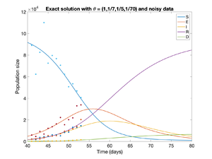
Example 1: To illustrate the previous concepts and notation we consider the SEIRD epidemiological deterministic model that describe the dynamics of the propagation of an infections disease, like COVID-19, [12]. If we have a closed constant population of ${\textstyle N}$ individuals, at each time ${\textstyle t}$ a compartmental model separates this population in five segments: susceptible, exposed, infectious, recovered and dead, denoted by ${\textstyle S(t)}$, ${\textstyle E(t)}$, ${\textstyle I(t)}$, ${\textstyle R(t)}$, ${\textstyle D(t)}$, respectively. The system of equations they satisfy is given by

${\frac {dS}{dt}}=-{\frac {\alpha }{N}}S\,I$ ${\frac {dE}{dt}}={\frac {\alpha }{N}}S\,I-\beta \,E$ ${\frac {dI}{dt}}=\beta \,E-{\frac {1}{T_{I}}}\,I$ (4) ${\frac {dR}{dt}}={\frac {1-f}{T_{I}}}\,I$ ${\frac {dD}{dt}}={\frac {f}{T_{I}}}\,I$

which is complemented with appropriate initial conditions, ${\textstyle S(t_{0})}$, ${\textstyle E(t_{0})}$, ${\textstyle I(t_{0})}$, ${\textstyle R(t_{0})}$, ${\textstyle D(t_{0})}$. In this system ${\textstyle \alpha }$ is the infection rate, ${\textstyle \beta }$ is the incubation rate, ${\textstyle T_{I}}$ is the average infectious period and ${\textstyle f}$ is the fraction of individuals who die. Here the dimension is ${\textstyle d=5}$ and the state variable is the vector ${\textstyle \mathbf {x} (t)=(S(t),E(t),I(t),R(t),D(t))^{T}}$, the number of parameters is ${\textstyle np=4}$ and ${\textstyle {\boldsymbol {\theta }}=(\alpha ,\beta ,T_{I},f)^{T}\sim (\alpha ,\beta ,\gamma ,\mu )^{T}}$ with ${\textstyle \gamma =1/T_{I}}$ and ${\textstyle \mu =f/T_{1}}$. Figure 1 shows the solution ${\textstyle \mathbf {x} (t)}$, obtained with the standard RK4 solver, of (1)–(5) in the time interval ${\textstyle [t_{0},t_{f}]=[40,80]}$ (days), with exact parameters ${\textstyle {\boldsymbol {\theta }}=(\alpha ,\beta ,\gamma ,\mu )^{T}=(1,1/7,1/5,1/70)^{T}}$, initial condition ${\textstyle \mathbf {x} _{0}=(91647,4853,1755,1620,125)^{T}}$ and total population ${\textstyle N=10^{5}}$. The points are experimental measurements at times ${\textstyle t_{i}=40+i}$, ${\textstyle 1\leq i\leq 13}$ (${\textstyle m=13}$). Of course, not always all variables are observable, as shown in this figure. Most frequently the observed variables reported by the medical or government agencies are those people in the population that have been infected, recovered and died, i.e. ${\textstyle {\overline {\mathbf {x} _{i}}}=(I_{i},R_{i},D_{i})}$ at times ${\textstyle t_{i}}$, so that the non-observable variables are ${\textstyle {\underline {\mathbf {x} }}_{i}=(S_{i},E_{i})}$.

Figure 1: The solution of the SEIRD model and synthetic measurements with white noise.

Assuming that the total population is constant or its change is negligible during the time period, then above system must be complemented by the conservation equation

$S(t)+E(t)+I(t)+R(t)+D(t)=N,\quad \forall \,t\in [t_{0},t_{f}],$

(5)

so (1)-(5) describe an differential-algebraic system. Accordingly, we may modify the optimization model (6), adding a penalized term, obtaining the extended model:

$L(\mathbf {x} _{0},{\boldsymbol {\theta }})={\frac {1}{2}}\left\Vert {\frac {\mathbf {x} _{0}-\mathbf {s} _{0}}{{\boldsymbol {\sigma }}_{0}}}\right\Vert _{5}^{2}+{\frac {k}{2}}(\mathbf {x} _{0}\cdot \mathbf {1} -N)^{2}+{\frac {1}{2}}\sum _{i=1}^{m}\left\Vert {\frac {{\overline {\mathbf {x} }}(t_{i};\mathbf {x} _{0},{\boldsymbol {\theta }})-{\overline {\mathbf {x} }}_{i}}{{\overline {\boldsymbol {\sigma }}}_{i}}}\right\Vert _{3}^{2},$

(6)

The penalty parameter ${\textstyle k}$ may be proportional to ${\textstyle N}$. The added penalized term in (6) helps stabilizing the optimization process to estimate the initial conditions. The constant vector ${\textstyle \mathbf {1} \in \mathbb {R} ^{d}}$ has components all equal to one, so the scalar product ${\textstyle \mathbf {x} _{0}\cdot \mathbf {1} }$ is equal to the sum of the components of ${\textstyle \mathbf {x} _{0}}$.

3 Variational approach

Our goal is to find the initial conditions ${\textstyle \mathbf {x} _{0}\in \mathbb {R} ^{d}}$ and the parameters ${\textstyle {\boldsymbol {\theta }}\in \mathbb {R} ^{np}}$ that minimize the cost function (6) subject to (1) and (5), given that we have a set of noisy experimental measurements (2) at different times. Since the model is deterministic and all the variables and functions are both continuous and smooth, we can employ gradient descent methods or quasi-Newton algorithms and its variants. The most expensive and delicate task, when applying these methods, is the calculation of the gradient or Jacobians of the cost function at each iteration. Some options are available to compute these quantities as shown in [3], [14], [4], and references therein. Here, we are interested on two approaches which are based on variational calculus.

Let ${\textstyle \mathbf {z} =(x_{0},{\boldsymbol {\theta }})^{T}\in \mathbb {R} ^{d+np}}$ be the vector which contain the unknown initial conditions and the unknown vector of parameters of the dynamical system, then to first order

$\nabla L(\mathbf {z} )\cdot \delta \mathbf {z} \approx L(\mathbf {z} +\delta \mathbf {z} )-L(\mathbf {z} )$

(7)

where ${\textstyle \delta \mathbf {z} =(\delta \mathbf {x} _{0},\delta {\boldsymbol {\theta }})^{T}}$ is an small increment of ${\textstyle \mathbf {z} }$. If we want to be more specific we can write

$\nabla _{\mathbf {x} _{0}}\,L(\mathbf {x} _{0},{\boldsymbol {\theta }})\cdot \delta \mathbf {x} _{0}+\nabla _{\theta }\,L(\mathbf {x} _{0},{\boldsymbol {\theta }})\cdot \delta {\boldsymbol {\theta }}\approx L(\mathbf {x} _{0}+\delta \mathbf {x} _{0},{\boldsymbol {\theta }}+\delta {\boldsymbol {\theta }})-L(\mathbf {x} _{0},{\boldsymbol {\theta }}),$

(8)

where ${\textstyle \nabla _{\mathbf {x} _{0}}}$ and ${\textstyle \nabla _{\theta }}$ denote the gradients with respect ${\textstyle \mathbf {x} _{0}}$ and ${\textstyle {\boldsymbol {\theta }}}$, receptively and the dot is used to denote the corresponding scalar products. Evaluating directly ${\textstyle L(\mathbf {x} _{0}+\delta \mathbf {x} _{0},{\boldsymbol {\theta }}+\delta {\boldsymbol {\theta }})}$ from (6), and simplifying, we obtain

$\nabla _{x_{0}}\,L(\mathbf {x} _{0},{\boldsymbol {\theta }})\cdot \delta \mathbf {x} _{0}+\nabla _{\theta }\,L(\mathbf {x} _{0},{\boldsymbol {\theta }})\cdot \delta {\boldsymbol {\theta }}\approx {\frac {\mathbf {x} _{0}-\mathbf {s} _{0}}{{\boldsymbol {\sigma }}_{0}^{2}}}\,\cdot \delta \mathbf {x} _{0}+k(\mathbf {x} _{0}\cdot \mathbf {1} -N)\,\mathbf {1} \cdot \delta \mathbf {x} _{0}$ $+\sum _{i=1}^{m}{\frac {{\overline {\mathbf {x} }}(t_{i};\mathbf {x} _{0},{\boldsymbol {\theta }})-{\overline {\mathbf {x} }}_{i}}{{\overline {\boldsymbol {\sigma }}}_{i}^{2}}}\cdot \left({\frac {\partial {\overline {\mathbf {x} }}(t_{i};\mathbf {x} _{0},{\boldsymbol {\theta }})}{\partial \mathbf {x} _{0}}}\delta \mathbf {x} _{0}+{\frac {\partial {\overline {\mathbf {x} }}(t_{i};\mathbf {x} _{0},{\boldsymbol {\theta }})}{\partial {\boldsymbol {\theta }}}}\delta {\boldsymbol {\theta }}\right).$

(9)

At the limit ${\textstyle \delta \mathbf {z} =(\delta \mathbf {x} _{0},\delta {\boldsymbol {\theta }})^{T}\rightarrow \mathbf {0} }$ we obtain the gradient ${\textstyle \nabla L(\mathbf {z} )=(\nabla _{x_{0}}\,L(\mathbf {x} _{0},{\boldsymbol {\theta }}),\nabla _{\theta }\,L(\mathbf {x} _{0},{\boldsymbol {\theta }}))^{T}}$ with the above derivatives distributed accordingly. In (9), matrices ${\textstyle \partial {\overline {\mathbf {x} }}(t_{i};\mathbf {x} _{0},{\boldsymbol {\theta }})/\partial \mathbf {x} _{0}}$ and ${\textstyle \partial {\overline {\mathbf {x} }}(t_{i};\mathbf {x} _{0},{\boldsymbol {\theta }})/\partial {\boldsymbol {\theta }}}$ are the Jacobians of the observable variables ${\textstyle {\overline {\mathbf {x} }}(t_{i};\mathbf {x} _{0},{\boldsymbol {\theta }})}$ with respect ${\textstyle \mathbf {x} _{0}}$ and ${\textstyle {\boldsymbol {\theta }}}$, respectively. In the literature, their partial derivatives are commonly called sensitivities of the observables, and their evaluation may require considerable computational effort. The first matrix is of size ${\textstyle no\times d}$ and the second matrix is of size ${\textstyle no\times np}$, then the total number of partial derivatives that we must compute in (9) is ${\textstyle m\times no(d+np)}$. For instance, in the above example for the SEIRD model, if the number of observable variables is ${\textstyle no=3}$, and there are ${\textstyle m=13}$ experimental measurements, we have to compute ${\textstyle 13\times 3(5+4)=351}$ sensitivities at each iteration of a typical gradient or quasi-Newton method. The most basic method to compute these derivatives is the finite difference method (see [14]), but it has some disadvantages. As mentioned before, we concentrate only in variational methods, which may be more sophisticated but they are commonly more efficient.

3.1 Variational method to compute the sensitivities

This method is also known as the forward approach, because a forward dynamical systems is solved to compute the sensitivities. We consider first the calculation of the sensitivities with respect to the parameter ${\textstyle {\boldsymbol {\theta }}}$, so let us denote the Jacobian ${\textstyle \partial \mathbf {x} (t;\mathbf {x} _{0},{\boldsymbol {\theta }})/\partial {\boldsymbol {\theta }}}$ by ${\textstyle J(t;\mathbf {x} _{0},{\boldsymbol {\theta }})}$ for simplicity. Then

$J(t;\mathbf {x} _{0},{\boldsymbol {\theta }})\,\delta {\boldsymbol {\theta }}\approx \mathbf {x} (t;\mathbf {x} _{0},{\boldsymbol {\theta }}+\delta {\boldsymbol {\theta }})-\mathbf {x} (t;\mathbf {x} _{0},{\boldsymbol {\theta }}).$

Taking derivatives with respect to ${\textstyle t}$, we obtain

${\dot {J}}(t;{\boldsymbol {\theta }})\,\delta {\boldsymbol {\theta }}\approx {\dot {\mathbf {x} }}(t;\mathbf {x} _{0},{\boldsymbol {\theta }}+\delta {\boldsymbol {\theta }})-{\dot {\mathbf {x} }}(t;\mathbf {x} _{0},{\boldsymbol {\theta }})$ $=\mathbf {f} (\mathbf {x} (t;\mathbf {x} _{0},{\boldsymbol {\theta }}+\delta {\boldsymbol {\theta }}),{\boldsymbol {\theta }}+\delta {\boldsymbol {\theta }})-\mathbf {f} (\mathbf {x} (t;\mathbf {x} _{0},{\boldsymbol {\theta }}),{\boldsymbol {\theta }})$ $\approx \mathbf {f} _{\mathbf {x} }(\mathbf {x} (t;\mathbf {x} _{0},{\boldsymbol {\theta }}),{\boldsymbol {\theta }})J(t;\mathbf {x} _{0},{\boldsymbol {\theta }})\,\delta {\boldsymbol {\theta }}+\mathbf {f} _{\boldsymbol {\theta }}(\mathbf {x} (t;\mathbf {x} _{0},{\boldsymbol {\theta }}),{\boldsymbol {\theta }})\,\delta {\boldsymbol {\theta }}.$

Then, ${\textstyle \mathbf {x} (t)=\mathbf {x} (t;\mathbf {x} _{0},{\boldsymbol {\theta }})}$ and ${\textstyle J(t)=J(t;\mathbf {x} _{0},{\boldsymbol {\theta }})}$ satisfy the following variational system:

${\dot {\mathbf {x} }}(t)=\mathbf {f} (\mathbf {x} (t),{\boldsymbol {\theta }}),\quad t_{0}<t\leq t_{f},$ $\mathbf {x} (t_{0})=\mathbf {x} _{0},$ ${\dot {J}}(t)=\mathbf {f} _{\mathbf {x} }(\mathbf {x} (t),{\boldsymbol {\theta }})J(t)+\mathbf {f} _{\boldsymbol {\theta }}(\mathbf {x} (t),{\boldsymbol {\theta }}),\quad t_{0}<t\leq t_{f},$ (10) $J(t_{0})=\mathbb {O} .$

Last two relations in (10) form a system of matricial differential equations and its initial condition reflects the fact that ${\textstyle \mathbf {x} _{0}}$ does not depend on ${\textstyle \theta }$, because

$J(t_{0})=J(t_{0};\mathbf {x} _{0},{\boldsymbol {\theta }})=\partial \mathbf {x} (t_{0};\mathbf {x} _{0},{\boldsymbol {\theta }})/\partial {\boldsymbol {\theta }}=\partial \mathbf {x} _{0}/\partial {\boldsymbol {\theta }}=\mathbb {O} \quad {\hbox{(the null matrix)}}.$

A similar variational system is satisfied by the matrix with the sensitivities with respect ${\textstyle \mathbf {x} _{0}}$. Therefore, with this approach, most of the computational work is concentrated in the solution of two matricial systems of differential equations and their evaluation at the experimental times ${\textstyle t_{i}}$, ${\textstyle 1\leq i\leq m}$. The amount of computational work will accumulate at each new iteration of the optimization algorithm, which in some cases may be prohibitive.

3.2 The adjoint method to compute the sensitivities

The total variation of ${\textstyle \mathbf {x} (t;\mathbf {x} _{0},{\boldsymbol {\theta }})}$ with respect to ${\textstyle \mathbf {x} _{0}}$ and ${\textstyle {\boldsymbol {\theta }}}$ is given by

$\delta \mathbf {x} (t;\mathbf {x} _{0},{\boldsymbol {\theta }})=\mathbf {x} (t;\mathbf {x} _{0}+\delta \mathbf {x} _{0},{\boldsymbol {\theta }}+\delta {\boldsymbol {\theta }})-\mathbf {x} (t;\mathbf {x} _{0},{\boldsymbol {\theta }})={\frac {\partial \mathbf {x} (t;\mathbf {x} _{0},{\boldsymbol {\theta }})}{\partial \mathbf {x} _{0}}}\delta \mathbf {x} _{0}+{\frac {\partial \mathbf {x} (t;\mathbf {x} _{0},{\boldsymbol {\theta }})}{\partial {\boldsymbol {\theta }}}}\delta {\boldsymbol {\theta }}.$

(11)

Our goal is to avoid the explicit calculation of the Jacobian matrices on the right hand side. Before we proceed further, let us first introduce the following Hilbert spaces:

$V=L^{2}([t_{0},t_{f}];\mathbb {R} ^{d})=\left\{\mathbf {v} :[t_{0},t_{f}]\rightarrow \mathbb {R} ^{d}\left\vert \int _{t_{0}}^{t_{f}}||\mathbf {v} (t)||^{2}\,dt<\infty \right.\right\},$ $H=H^{1}([t_{0},t_{f}];\mathbb {R} ^{d})=\{\mathbf {v} \in V|d\mathbf {v} /dt\in V\},$

where the ${\textstyle ||\mathbf {v} (t)||^{2}=\mathbf {v} (t)^{T}\mathbf {v} (t)=\mathbf {v} (t)\cdot \mathbf {v} (t)}$ is the usual scalar product in ${\textstyle \mathbb {R} ^{d}}$. Then a natural inner product in ${\textstyle V}$ is given by ${\textstyle \langle \mathbf {u} ,\mathbf {v} \rangle =\int _{t_{0}}^{t_{f}}\mathbf {u} (t)\cdot \mathbf {v} (t)\,dt}$ with induced norm given by ${\textstyle \Vert \mathbf {u} \Vert _{V}=\langle \mathbf {u} ,\mathbf {u} \rangle ^{1/2}}$.

Since ${\textstyle \mathbf {x} (t)=\mathbf {x} (t;\mathbf {x} _{0},{\boldsymbol {\theta }})\in H}$ satisfies the state equation (1), then the following inner product is null

$\int _{t_{0}}^{t_{f}}\left({\dot {\mathbf {x} }}(t)-\mathbf {f} (\mathbf {x} (t),\mathbf {x} _{0},{\boldsymbol {\theta }})\right)\cdot \mathbf {p} (t)\,dt=0,\quad \forall \mathbf {p} \in H.$

Differentiating this expression, we get

$\int _{t_{0}}^{t_{f}}\!\!\delta {\dot {\mathbf {x} }}(t)\cdot \mathbf {p} (t)\,dt=\int _{t_{0}}^{t_{f}}\!\!\left[\,\mathbf {f} _{\mathbf {x} }(\mathbf {x} (t),\mathbf {x} _{0},{\boldsymbol {\theta }})\,\delta \mathbf {x} (t)+\mathbf {f} _{\mathbf {x} _{0}}(\mathbf {x} (t),\mathbf {x} _{0},{\boldsymbol {\theta }})\,\delta \mathbf {x} _{0}+\mathbf {f} _{\boldsymbol {\theta }}(\mathbf {x} (t),\mathbf {x} _{0},{\boldsymbol {\theta }})\,\delta {\boldsymbol {\theta }}\,\right]\cdot \mathbf {p} (t)\,dt,$

where ${\textstyle \mathbf {f} _{\mathbf {x} }}$, ${\textstyle \mathbf {f} _{\mathbf {x} _{0}}}$ and ${\textstyle \mathbf {f} _{\boldsymbol {\theta }}}$ are the Jacobians of ${\textstyle \mathbf {f} }$ with respect to ${\textstyle \mathbf {x} }$, ${\textstyle \mathbf {x} _{0}}$ and ${\textstyle {\boldsymbol {\theta }}}$, respectively. Integrating by parts the left hand side, and observing that on the right hand side ${\textstyle \left[\mathbf {f} _{\mathbf {x} }\,\delta \mathbf {x} \right]\cdot \mathbf {p} =\left[\mathbf {f} _{\mathbf {x} }^{T}\,\mathbf {p} \right]\cdot \delta \mathbf {x} }$, ${\textstyle \left[\mathbf {f} _{\boldsymbol {\theta }}\,\delta \mathbf {x} _{0}\right]\cdot \mathbf {p} =\left[\mathbf {f} _{\boldsymbol {\theta }}^{T}\,\mathbf {p} \right]\cdot \delta \mathbf {x} _{0}}$, and ${\textstyle \left[\mathbf {f} _{\boldsymbol {\theta }}\,\delta {\boldsymbol {\theta }}\right]\cdot \mathbf {p} =\left[\mathbf {f} _{\boldsymbol {\theta }}^{T}\,\mathbf {p} \right]\cdot \delta {\boldsymbol {\theta }}}$, we obtain

$\mathbf {p} (t)\!\cdot \!\delta \mathbf {x} (t)|_{t_{0}}^{t_{f}}-\int _{t_{0}}^{t_{f}}\!\!\!{\dot {\mathbf {p} }}(t)\!\cdot \!\delta \mathbf {x} (t)\,dt=\int _{t_{0}}^{t_{f}}\!\!\left\{\left[\mathbf {f} _{\mathbf {x} }^{T}\,\mathbf {p} \right](t)\!\cdot \!\delta \mathbf {x} (t)+\left[\mathbf {f} _{\mathbf {x} _{0}}^{T}\,\mathbf {p} \right](t)\!\cdot \!\delta \mathbf {x} _{0}(t)+\left[\mathbf {f} _{\boldsymbol {\theta }}^{T}\,\mathbf {p} \right](t)\!\cdot \!\delta {\boldsymbol {\theta }}\right\}dt,$

and, assuming that ${\textstyle \mathbf {f} }$ does not depend explicitly of ${\textstyle \mathbf {x} _{0}}$ (it depends only through ${\textstyle \mathbf {x} }$, but the variation w.r.t. ${\textstyle \mathbf {x} _{0}}$ is already accounted in ${\textstyle \delta \mathbf {x} }$), then

$\mathbf {p} (t)\cdot \delta \mathbf {x} (t)|_{t_{0}}^{t_{f}}-\int _{t_{0}}^{t_{f}}\left\{{\dot {\mathbf {p} }}(t)+\left[\mathbf {f} _{\mathbf {x} }^{T}\,\mathbf {p} \right](t)\right\}\cdot \delta \mathbf {x} (t)\,dt=\int _{t_{0}}^{t_{f}}\left[\mathbf {f} _{\boldsymbol {\theta }}^{T}\,\mathbf {p} \right](t)\cdot \delta {\boldsymbol {\theta }}\,dt,$

(12)

where ${\textstyle \delta \mathbf {x} }$ is given by (11) and arise in the last term of (9). One way to avoid the explicit computation of (11) is forcing a relation with (12) by introducing the following adjoint equation

$-{\dot {\mathbf {p} }}(t)=\mathbf {f} _{\mathbf {x} }(\mathbf {x} (t),{\boldsymbol {\theta }})^{T}\,\mathbf {p} (t)+\sum _{i=1}^{m}{\frac {({\overline {\mathbf {x} }}(t_{i};\mathbf {x} _{0},{\boldsymbol {\theta }})-{\overline {\mathbf {x} }}_{i})}{{\overline {\boldsymbol {\sigma }}}_{i}^{2}}}\,{\boldsymbol {\delta }}_{\mathbf {D} }(t-t_{i}),t_{f}>t\geq t_{0},$ $\mathbf {p} (t_{f})=\mathbf {0} ,$

(13)

with ${\textstyle {\boldsymbol {\delta }}_{\mathbf {D} }(t-t_{i})}$ the Dirac measure centred at ${\textstyle t_{i}}$. This adjoint equation (a backward in time differential equation) contains all the information about the experimental data ${\textstyle \{{\overline {\mathbf {x} }}_{i}\}_{i=1}^{m}}$, and its variational formulation is obtained multiplying by a differentiable test function ${\textstyle {\boldsymbol {\phi }}(t)}$ and integrating:

$-\int _{t_{0}}^{t_{f}}\left\{{\dot {\mathbf {p} }}(t)+\left[\mathbf {f} _{\mathbf {x} }^{T}\,\mathbf {p} \right](t)\right\}\cdot {\boldsymbol {\phi }}(t)\,dt=\int _{t_{0}}^{t_{f}}\sum _{i=1}^{m}{\frac {({\overline {\mathbf {x} }}(t_{i};\mathbf {x} _{0},{\boldsymbol {\theta }})-{\overline {\mathbf {x} }}_{i})}{{\overline {\boldsymbol {\sigma }}}_{i}^{2}}}\,{\boldsymbol {\delta }}_{\mathbf {D} }(t-t_{i})\cdot {\boldsymbol {\phi }}(t)\,dt.$

(14)

The integral on the right hand side is equal to ${\textstyle \sum _{i=1}^{m}{\frac {({\overline {\mathbf {x} }}(t_{i};\mathbf {x} _{0},{\boldsymbol {\theta }})-{\overline {\mathbf {x} }}_{i})}{{\overline {\boldsymbol {\sigma }}}_{i}}}\cdot {\boldsymbol {\phi }}(t_{i})}$. Choosing ${\textstyle {\boldsymbol {\phi }}(t)=\delta \mathbf {x} (t)}$ in (14) and substituting the result in (12), we obtain

$-\mathbf {p} (t_{0})\cdot \delta \mathbf {x} (t_{0})+\sum _{i=1}^{m}{\frac {({\overline {\mathbf {x} }}(t_{i};\mathbf {x} _{0},{\boldsymbol {\theta }})-{\overline {\mathbf {x} }}_{i})}{{\overline {\boldsymbol {\sigma }}}_{i}^{2}}}\cdot \delta \mathbf {x} (t_{i})=\int _{t_{0}}^{t_{f}}\left[\mathbf {f} _{\boldsymbol {\theta }}^{T}\,\mathbf {p} \right](t)\cdot \delta {\boldsymbol {\theta }}\,dt,$

(15)

where ${\textstyle \mathbf {p} (t)}$ is the solution of the adjoint equation. Finally, the substitution of this equation into (9), gives

$\nabla _{x_{0}}\,L(\mathbf {x} _{0},{\boldsymbol {\theta }})\cdot \delta \mathbf {x} _{0}+\nabla _{\theta }\,L(\mathbf {x} _{0},{\boldsymbol {\theta }})\cdot \delta {\boldsymbol {\theta }}$ $\approx {\frac {\mathbf {x} _{0}-\mathbf {s} _{0}}{{\boldsymbol {\sigma }}_{0}^{2}}}\,\cdot \delta \mathbf {x} _{0}+k(\mathbf {x} _{0}\cdot \mathbf {1} -N)\,\mathbf {1} \cdot \delta \mathbf {x} _{0}+\mathbf {p} (t_{0})\cdot \delta \mathbf {x} _{0}+\left[\int _{t_{0}}^{t_{f}}\left[\mathbf {f} _{\boldsymbol {\theta }}^{T}\,\mathbf {p} \right](t)\,dt\right]\cdot \delta {\boldsymbol {\theta }}.$

(16)

Therefore, the gradient of the objective function (6) is ${\textstyle \nabla L(\mathbf {z} )=(\nabla _{x_{0}}L(\mathbf {x} _{0},{\boldsymbol {\theta }}),\nabla _{\boldsymbol {\theta }}L(\mathbf {x} _{0},{\boldsymbol {\theta }}))^{T}}$, with

$\nabla _{x_{0}}L(\mathbf {x} _{0},{\boldsymbol {\theta }})={\frac {\mathbf {x} _{0}-\mathbf {s} _{0}}{{\boldsymbol {\sigma }}_{0}^{2}}}+k(\mathbf {x} _{0}\cdot \mathbf {1} -N)\,\mathbf {1} +\mathbf {p} (t_{0}),$ (17) $\nabla _{\boldsymbol {\theta }}L(\mathbf {x} _{0},{\boldsymbol {\theta }})=\int _{t_{0}}^{t_{f}}\mathbf {f} _{\boldsymbol {\theta }}(\mathbf {x} (t),\mathbf {x} _{0},{\boldsymbol {\theta }})^{T}\,\mathbf {p} (t)\,dt,$ (18)

where ${\textstyle \mathbf {x} (t)}$ solves the state equation (1) and ${\textstyle \mathbf {p} (t)}$ solves the adjoint equation (13).

Remark 3: Formulas (17)-(18) avoid the explicit calculation of the sensitivities, they only requiere the solution of the state equation (1) and of the adjoint equation (13), regardless of the number of experimental data, ${\textstyle m}$, the number of parameters, ${\textstyle np}$, and of the observable variables, ${\textstyle no}$. Furthermore, these same equations must be solved to compute either the gradient with respect ${\textstyle \mathbf {x} _{0}}$ or with respect ${\textstyle {\boldsymbol {\theta }}}$, or both gradients simultaneously.

Remark 4: The solution of the adjoint equation turns out to be the Lagrange multiplier of the optimization problem, with objective function ${\textstyle L(\mathbf {x} _{0},{\boldsymbol {\theta }})}$, subject to the constraint (1). To show this property, let us introduce the Lagrangian function

${\mathcal {L}}(\mathbf {x} _{0},{\boldsymbol {\theta }},\mathbf {p} )=L(\mathbf {x} _{0},{\boldsymbol {\theta }})+\int _{t_{0}}^{t_{f}}\mathbf {p} (t)^{T}\left[\mathbf {f} (t,\mathbf {x} (t),{\boldsymbol {\theta }})-{\dot {\mathbf {x} }}(t)\right]\,dt,$

(19)

where ${\textstyle \mathbf {p} }$ is the Lagrange multiplier associated to the given constraint, and the last term is the inner product of this multiplier with the restriction. Our goal is to compute ${\textstyle \partial L/\partial {\boldsymbol {\theta }}}$ from this expression. Formally, the second term on the right hand side of (4) is zero because the state ${\textstyle \mathbf {x} (t)}$ solves the ODE, therefore ${\textstyle \partial {\mathcal {L}}/\partial {\boldsymbol {\theta }}=\partial L/\partial {\boldsymbol {\theta }}}$. However, the differentiation of ${\textstyle {\mathcal {L}}}$ reveals additional information and gives more freedom. Doing integration by parts of the term ${\textstyle -\int _{t_{0}}^{t_{f}}\mathbf {p} (t)^{T}{\dot {\mathbf {x} }}(t)}$ in (4) first, and then taking the derivative with respect to ${\textstyle {\boldsymbol {\theta }}}$, we obtain

${\frac {\partial {\mathcal {L}}}{\partial {\boldsymbol {\theta }}}}={\frac {\partial L}{\partial {\boldsymbol {\theta }}}}-\left.\mathbf {p} ^{T}{\frac {\partial \mathbf {x} }{\partial {\boldsymbol {\theta }}}}\right|_{t_{0}}^{t_{f}}+\int _{t_{0}}^{t_{f}}\!\!{\dot {\mathbf {p} }}^{T}{\frac {\partial \mathbf {x} }{\partial {\boldsymbol {\theta }}}}dt+\int _{t_{0}}^{t_{f}}\!\!\mathbf {p} ^{T}\left[\mathbf {f} _{\mathbf {x} }{\frac {\partial \mathbf {x} }{\partial {\boldsymbol {\theta }}}}+\mathbf {f} _{\boldsymbol {\theta }}\right]dt$ $=\sum _{i=1}^{m}\left({\frac {{\overline {\mathbf {x} }}(t_{i},\mathbf {x} _{0},{\boldsymbol {\theta }})-{\overline {\mathbf {x} }}_{i}}{{\overline {\boldsymbol {\sigma }}}_{i}^{2}}}\right)^{T}\!\!{\frac {\partial {\overline {\mathbf {x} }}}{\partial \theta }}-\left.\mathbf {p} ^{T}{\frac {\partial \mathbf {x} }{\partial {\boldsymbol {\theta }}}}\right|_{t_{0}}^{t_{f}}+\int _{t_{0}}^{t_{f}}\!\!\left({\dot {\mathbf {p} }}+\mathbf {f} _{\mathbf {x} }^{T}\mathbf {p} \right)^{T}{\frac {\partial \mathbf {x} }{\partial {\boldsymbol {\theta }}}}dt+\int _{t_{0}}^{t_{f}}\!\!\mathbf {p} ^{T}\mathbf {f} _{\boldsymbol {\theta }}\,dt.$

(20)

The first term on the right hand side is obtained directly from (6) and can be expressed as

$\sum _{i=1}^{m}\left({\frac {{\overline {\mathbf {x} }}(t_{i},\mathbf {x} _{0},{\boldsymbol {\theta }})-{\overline {\mathbf {x} }}_{i}}{{\overline {\boldsymbol {\sigma }}}_{i}^{2}}}\right)^{T}\!\!{\frac {\partial {\overline {\mathbf {x} }}}{\partial \theta }}=\int _{t_{0}}^{t_{f}}\sum _{i=1}^{m}\left({\frac {{\overline {\mathbf {x} }}(t_{i},\mathbf {x} _{0},{\boldsymbol {\theta }})-{\overline {\mathbf {x} }}_{i}}{{\overline {\boldsymbol {\sigma }}}_{i}^{2}}}\right)^{T}\!\!{\frac {\partial {\overline {\mathbf {x} }}}{\partial \theta }}\,\delta _{D}(t-t_{i})dt.$

Now, if ${\textstyle \mathbf {p} }$ satisfies the adjoint equation (13) then the sum of first and third terms in (20) vanish, and also the boundary term ${\textstyle \left.\mathbf {p} ^{T}{\frac {\partial \mathbf {x} }{\partial {\boldsymbol {\theta }}}}\right|_{t_{0}}^{t_{f}}}$, since ${\textstyle \mathbf {p} (t_{f})=\mathbf {0} }$ and ${\textstyle \partial \mathbf {x} (t_{0})/\partial {\boldsymbol {\theta }}=\mathbb {O} }$. Therefore

${\frac {\partial {\mathcal {L}}}{\partial {\boldsymbol {\theta }}}}={\frac {\partial L}{\partial {\boldsymbol {\theta }}}}=\int _{t_{0}}^{t_{f}}\mathbf {p} ^{T}\mathbf {f} _{\boldsymbol {\theta }}\,dt\quad \Longrightarrow \quad \nabla _{\boldsymbol {\theta }}L(\mathbf {x} _{0},{\boldsymbol {\theta }})=\int _{t_{0}}^{t_{f}}\mathbf {f} _{\boldsymbol {\theta }}(t,\mathbf {x} (t),{\boldsymbol {\theta }})^{T}\,\mathbf {p} (t)\,dt.$

A similar development can be applied to obtain ${\textstyle \partial L/\partial \mathbf {x} _{0}}$.

3.3 Solution of the adjoint equation and computation of the gradient

The adjoint equation (13) is a system of ODE with backward in time propagation. We apply a change of variable from the symmetric relation ${\textstyle t_{f}-\tau =t-t_{0}}$:

$p(t)=p(t_{f}-(\tau {-}t_{0}))\equiv p_{A}(\tau )\quad \Longrightarrow \quad {\dot {p}}(t)=-{\dot {p}}_{A}(\tau ),$

(21)

obtaining the equivalent system with forward in time dynamics

${\dot {\mathbf {p} }}_{A}(\tau )=\mathbf {f} _{\mathbf {x} }(\mathbf {x} _{A}(\tau ),{\boldsymbol {\theta }})^{T}\,\mathbf {p} _{A}(\tau )+\sum _{i=1}^{m}{\frac {{\overline {\mathbf {x} }}_{A}(\tau _{i},\mathbf {x} _{0},{\boldsymbol {\theta }})-{\overline {\mathbf {x} }}_{m+1-i}}{{\overline {\boldsymbol {\sigma }}}_{m+1-i}^{2}}}\,\delta _{D}(\tau _{i}-\tau ),\quad t_{0}\leq \tau <t_{f},$ (22) $\mathbf {p} _{A}(\tau _{0})=\mathbf {0} ,$ (23)

which can be solved with any usual numerical ODE solver like Runge–Kutta methods.

For the SEIRD model, if the observable variables are ${\textstyle {\overline {\mathbf {x} }}(t)=(I(t),R(t),D(t))^{T}}$, the adjoint equation (22) takes the form

$\left[\!\!{\begin{array}{c}{\dot {p}}_{_{A1}}(\tau )\\{\dot {p}}_{_{A2}}(\tau )\\{\dot {p}}_{_{A3}}(\tau )\\{\dot {p}}_{_{A4}}(\tau )\\{\dot {p}}_{_{A5}}(\tau )\end{array}}\!\!\right]=\left[\!\!{\begin{array}{ccrcr}-{\frac {\alpha \,I(\tau )}{N}}&{\frac {\alpha \,I(\tau )}{N}}&0&0&0\\0&-\beta &\beta &0&0\\-{\frac {\alpha \,S(\tau )}{N}}&{\frac {\alpha \,S(\tau )}{N}}&-\gamma &\gamma -\mu &\mu \\0&0&0&0&0\\0&0&0&0&0\end{array}}\!\!\right]\!\!\left[\!\!{\begin{array}{c}p_{_{A1}}(\tau )\\p_{_{A2}}(\tau )\\p_{_{A3}}(\tau )\\p_{_{A4}}(\tau )\\p_{_{A5}}(\tau )\end{array}}\!\!\right]+\left[\!\!{\begin{array}{c}0\\0\\\sum _{i=1}^{m}{\frac {I(\tau _{i})-I_{m+1-i}}{\sigma _{i3}^{2}}}\delta _{D}(\tau _{i}-\tau )\\\sum _{i=1}^{m}{\frac {R(\tau _{i})-R_{m+1-i}}{\sigma _{i4}^{2}}}\delta _{D}(\tau _{i}-\tau )\\\sum _{i=1}^{m}{\frac {D(\tau _{i})-D_{m+1-i}}{\sigma _{i5}^{2}}}\delta _{D}(\tau _{i}-\tau )\end{array}}\!\!\right],$

with ${\textstyle \gamma =1/T_{1}}$, ${\textstyle \mu =f/T_{1}}$ in (1). After solving this forward adjoint equation we recover the solution ${\textstyle \mathbf {p} }$ of the backward adjoint equation (13) with ${\textstyle \mathbf {p} (t_{i})=\mathbf {p} _{A}(\tau _{m+1-i})}$, ${\textstyle i=1,\ldots ,m}$ or by interpolation and using (21) for other values of ${\textstyle t}$.

The last step to compute the gradient is the calculation of the integral in (18). Observe that

$\mathbf {f} _{\boldsymbol {\theta }}(\mathbf {x} (t),{\boldsymbol {\theta }})^{T}\,\mathbf {p} (t)=\left[\!\!{\begin{array}{rrrr}-{\dfrac {S(t)\,I(t)}{N}}&{\dfrac {S(t)\,I(t)}{N}}&0&0\\0&-E(t)&E(t)&0\\0&0&-I(t)&I(t)\end{array}}\!\!\right]\left[\!\!{\begin{array}{c}p_{1}(t)\\p_{2}(t)\\p_{3}(t)\\p_{4}(t)\end{array}}\!\!\right]$ $=\left[{\begin{array}{c}{\dfrac {S(t)\,I(t)}{N}}\,(p_{2}(t)-p_{1}(t))\\E(t)\,(p_{3}(t)-p_{2}(t))\\I(t)\,(p_{4}(t)-p_{3}(t))\end{array}}\right]\equiv \mathbf {H} (t)$

Then, using the Simpson's rule in a set of given times (nodes of the mesh or interpolated times) we have

$\int _{t_{0}}^{t_{f}}\mathbf {f} _{\boldsymbol {\theta }}(\mathbf {x} (t),{\boldsymbol {\theta }})^{T}\,\mathbf {p} (t)\,dt={\frac {\Delta t}{6}}\sum _{j=1}^{N-1}\left\{\mathbf {H} (t_{j-1})+4\mathbf {H} (t_{j})+\mathbf {H} (t_{j+1})\right\}$

(24)

4 Numerical algorithms for the optimization problem

4.1 Conjugate gradient algorithm

This algorithm is one of the most important algorithms for quadratic optimization problems with positive definite Hessians and for unconstrained continuous convex optimization. It may be considered as a variant of gradient descent where the search directions are generated progressively based on the orthogonality of the residuals and conjugacy of the search directions. The conjugate directions are calculated at each iteration a linear combination of the most recent negative gradient and the last conjugate direction, as indicated in step 9 of Algorithm 1 bellow. Its computational cost is comparable to steepest descent, but it has faster convergence, specially for ill conditioned problems, [9].

Initialization 1. Initial guess ${\textstyle \mathbf {z} ^{0}={\widehat {\mathbf {z} }}=({\widehat {\mathbf {x} }}_{0},{\widehat {\boldsymbol {\theta }}})^{T}}$. 2. Initial gradient ${\textstyle \mathbf {g} ^{0}=\nabla L(\mathbf {z} ^{0})}$. 3. Initial direction ${\textstyle \mathbf {d} ^{0}=-\mathbf {g} ^{0}}$. Descent For ${\textstyle \ell \geq 0}$, given ${\textstyle \mathbf {z} ^{\ell }}$, ${\textstyle \mathbf {g} ^{\ell }}$, ${\textstyle \mathbf {d} ^{\ell }}$, find ${\textstyle \mathbf {z} ^{\ell {+1}}}$, ${\textstyle \mathbf {g} ^{\ell {+1}}}$, ${\textstyle \mathbf {d} ^{\ell {+1}}}$, doing the following 4. Find ${\textstyle \rho _{\ell }=\displaystyle \arg \min _{\rho \geq 0}\varphi (\rho )=L(\mathbf {z} ^{\ell }+\rho \,\mathbf {d} ^{\ell })}$ 5. Update ${\textstyle \mathbf {z} ^{\ell {+1}}=\mathbf {z} ^{\ell }+\rho _{\ell }\,\mathbf {d} ^{\ell }}$. 6. Evaluate ${\textstyle \mathbf {g} ^{\ell +1}=\nabla L(\mathbf {z} ^{\ell +1})}$ Convergence test and new direction $\Vert \mathbf {g} ^{\ell +1}\Vert \leq \epsilon \Vert \mathbf {g} ^{0}\Vert$ 7. Take $\mathbf {z} ^{*}=\mathbf {z} ^{\ell +1}$. Stop and exit. 8. Evaluate $\beta _{\ell }={\dfrac {\mathbf {g} ^{\ell +1}\cdot \mathbf {g} ^{\ell +1}}{\mathbf {g} ^{\ell }\cdot \mathbf {g} ^{\ell }}}$9. Update $\mathbf {d} ^{\ell +1}=-\mathbf {g} ^{\ell }+\beta _{\ell }\,\mathbf {d} ^{\ell }$10. Make $\ell =\ell +1$ and go back to 4.

Algorithm. 1 Conjugate gradient algorithm

If ${\textstyle \beta _{\ell }=0}$ for all ${\textstyle \ell }$ we recover steepest descent. Some variants for computing ${\textstyle \beta _{\ell }\neq 0}$, include:

${\begin{array}{ll}\bullet {\hbox{Fletcher--Reeves: }}\beta _{\ell }={\dfrac {\mathbf {g} ^{\ell +1}\cdot \mathbf {g} ^{\ell +1}}{\mathbf {g} ^{\ell }\cdot \mathbf {g} ^{\ell }}}&\quad \bullet {\hbox{ Polak--Ribiere: }}\beta _{\ell }={\dfrac {\mathbf {g} ^{\ell {+1}}\cdot (\mathbf {g} ^{\ell {+1}}-\mathbf {g} ^{\ell })}{\mathbf {g} ^{\ell }\cdot \mathbf {g} ^{\ell }}}\\\bullet {\hbox{ Hestenes--Stiefel: }}\beta _{\ell }={\dfrac {\mathbf {g} ^{\ell {+1}}\cdot (\mathbf {g} ^{\ell {+1}}-\mathbf {g} ^{\ell })}{\mathbf {d} ^{\ell }\cdot (\mathbf {g} ^{\ell {+1}}-\mathbf {g} ^{\ell })}}&\quad \bullet {\hbox{ Dai--Yuan: }}\beta _{\ell }={\dfrac {\mathbf {g} ^{\ell +1}\cdot \mathbf {g} ^{\ell +1}}{\mathbf {d} ^{\ell }\cdot (\mathbf {g} ^{\ell {+1}}-\mathbf {g} ^{\ell })}}\end{array}}$

We use the short notations F–R, P–R, H–S, D–Y, for these variants.

4.2 BFGS algorithm

This is one of the most popular quasi-Newton algorithms for nonlinear optimization. It is usually more effective because it involves information about curvature, besides the information about the gradient. The curvature information is incorporated by approximating the Hessian matrix during the iteration process, which formaly plays the role of preconditioner for the gradient. The general idea about these methods comes from the second order approximation:

$L(\mathbf {z} ^{\ell }+\Delta \mathbf {z} )\approx L(\mathbf {z} ^{\ell })+\nabla L(\mathbf {z} ^{\ell })^{T}\Delta \mathbf {z} +{\frac {1}{2}}\Delta \mathbf {z} ^{T}A\,\Delta \mathbf {z} ,$

with a matrix ${\textstyle A}$ close to the Hessian. Then the so called secant condition is obtained:

$\nabla L(\mathbf {z} ^{\ell }+\Delta \mathbf {z} )\approx \nabla L(\mathbf {z} ^{\ell })+A\,\Delta \mathbf {z} .$

Forcing the gradient to be zero (to look for a minimum), we obtain the Newton step

$\Delta \mathbf {z} =-H\,\nabla L(\mathbf {z} ^{\ell }),\quad {\hbox{where}}\quad H\approx A^{-1}$

and the following search direction ${\textstyle \mathbf {d} ^{\ell }}$ is obtained;

$\mathbf {d} ^{\ell }=-H\,\mathbf {g} ^{\ell },\quad {\hbox{with}}\quad \mathbf {d} ^{\ell }=\Delta \mathbf {z} ,\quad \mathbf {g} ^{\ell }=\nabla L(\mathbf {z} ^{\ell }{).}$

The Hessian and its inverse are updated at every iteration adding rank–one or rank–two matrices. The BFGS algorithm updates the approximated Hessian with a rank–two matrix as showing in step 9 of Algorithm 2 bellow.

Initialization 1. Initial guess ans initial Hessian: ${\textstyle \mathbf {z} ^{0}}$ given, and ${\textstyle H^{0}=I}$. 2. Initial gradient ${\textstyle \mathbf {g} ^{0}=\nabla L(\mathbf {z} ^{0})}$. 3. Initial direction ${\textstyle \mathbf {d} ^{0}=-\mathbf {g} ^{0}}$. Descent For ${\textstyle \ell \geq 0}$, given ${\textstyle \mathbf {z} ^{\ell }}$, ${\textstyle \mathbf {g} ^{\ell }}$, ${\textstyle \mathbf {d} ^{\ell }}$, ${\textstyle H^{\ell }}$ find ${\textstyle \mathbf {z} ^{\ell {+1}}}$, ${\textstyle \mathbf {g} ^{\ell {+1}}}$, ${\textstyle \mathbf {d} ^{\ell {+1}}}$, ${\textstyle H^{\ell +1}}$, doing the following 4. Find ${\textstyle \rho _{\ell }=\displaystyle \arg \min _{\rho \geq 0}\varphi (\rho )=L(\mathbf {z} ^{\ell }+\rho \,\mathbf {d} ^{\ell })}$ 5. Update ${\textstyle \mathbf {z} ^{\ell {+1}}=\mathbf {z} ^{\ell }+\rho _{\ell }\,\mathbf {d} ^{\ell }}$. 6. Evaluate ${\textstyle \mathbf {g} ^{\ell +1}=\nabla L(\mathbf {z} ^{\ell +1})}$ Convergence test and new direction $\Vert \mathbf {g} ^{\ell +1}\Vert \leq \epsilon \Vert \mathbf {g} ^{0}\Vert$ 7. Do $\mathbf {z} ^{*}=\mathbf {z} ^{\ell +1}$. Stop and exit. 8. Evaluate $\mathbf {u} =\Delta \mathbf {z} ^{\ell }=\mathbf {z} ^{\ell +1}-\mathbf {z} ^{\ell }$ and $\mathbf {v} =\Delta \mathbf {g} ^{\ell }=\mathbf {g} ^{\ell +1}-\mathbf {g} ^{\ell }$ 9. Update $\displaystyle H^{\ell {+1}}=\left(I-{\frac {\mathbf {v} \mathbf {u} ^{T}}{\mathbf {u} ^{T}\mathbf {v} }}\right)H^{\ell }\left(I-{\frac {\mathbf {u} \mathbf {v} ^{T}}{\mathbf {u} ^{T}\mathbf {v} }}\right)+{\frac {\mathbf {v} \mathbf {v} ^{T}}{\mathbf {u} ^{T}\mathbf {v} }}$ 10. Update $\mathbf {d} ^{\ell +1}=-H^{\ell {+1}}\mathbf {g} ^{\ell +1}$ 11. Make $\ell =\ell +1$ and go back to 4

Algorithm. 2 BFGS algorithm

Remark 5: Another very popular method for least squares problems is the Gauss-Newton method and it variant, the Levenverg-Marquadt method (see [9]), where the Jacobian of the residual vector ${\textstyle \mathbf {r} =\left\{\left\Vert {\frac {{\overline {\mathbf {x} }}(t_{i};\mathbf {x} _{0},{\boldsymbol {\theta }})-{\overline {\mathbf {x} }}_{i}}{{\overline {\boldsymbol {\sigma }}}_{i}}}\right\Vert ^{2}\right\}_{i=1}^{m}}$ with respect to ${\textstyle \mathbf {x} _{0}}$ and ${\textstyle {\boldsymbol {\theta }}}$ must be computed at each iteration. These partial derivatives can also be computed with variational methods.

4.3 Line search

The most critical step in Algorithms 1 and 2 is the solution of the one dimensional optimization problem at step 4. This is not a trivial step and requires careful treatment. There are several algorithms for this problem, the most common are line search methods and trust region methods. Some classic references are [8] and [9], or the more recent one [15], while some publications, e,g, [1] and [10], show that this topic is still under development.

Given that we have a efficient way to compute the derivative ${\textstyle \varphi ^{\prime }(\rho )=\nabla L(\mathbf {z} ^{\ell }+\rho \,\mathbf {d} ^{\ell })\cdot \mathbf {d} ^{\ell }}$, we may use the secant method, whose iteration formula is

$\rho _{k+1}=\rho _{k}-{\frac {\varphi ^{\,\prime }(\rho _{k})(\rho _{k}-\rho _{k-1})}{\varphi ^{\,\prime }(\rho _{k})-\varphi ^{\,\prime }(\rho _{k-1})}}={\frac {\rho _{k-1}\varphi ^{\,\prime }(\rho _{k})-\rho _{k}\varphi ^{\,\prime }(\rho _{k-1})}{\varphi ^{\,\prime }(\rho _{k})-\varphi ^{\,\prime }(\rho _{k-1})}},\qquad k=1,2,\ldots$

(25)

with two initial values ${\textstyle \rho _{0}=0}$ and ${\textstyle \rho _{1}\approx \epsilon \,{\frac {||\mathbf {z} ||}{||\mathbf {d} ||}}}$, ${\textstyle \epsilon <1}$. The initial value ${\textstyle \rho _{1}}$ takes into account a proper scaling (see step 5). Computing ${\textstyle \varphi ^{\,\prime }(\rho )}$ requires solving the state equation (1) with initial conditions ${\textstyle \mathbf {x} _{0}^{\ell }+\rho \mathbf {d} _{0}^{\ell }}$ and parameter ${\textstyle {\boldsymbol {\theta }}^{\ell }+\rho \mathbf {d} _{\boldsymbol {\theta }}^{\ell }}$, obtaining a solution that we call ${\textstyle \mathbf {x} _{\rho }^{\ell }}$, and then solving the corresponding adjoint equation (13) with ${\textstyle \mathbf {x} =\mathbf {x} _{\rho }^{\ell }}$ and ${\textstyle {\boldsymbol {\theta }}={\boldsymbol {\theta }}^{\ell }+\rho \mathbf {d} _{\boldsymbol {\theta }}^{\ell }}$, obtaining the solution ${\textstyle \mathbf {p} _{\rho }^{\ell }}$. Thus

$\varphi ^{\,\prime }(\rho )\!=\!\left[\!\!{\begin{array}{c}\mathbf {p} _{\rho }^{\ell }(t_{0})+{\dfrac {{\overline {\mathbf {x} }}_{0}^{\ell }+\rho \,{\overline {\mathbf {d} }}_{0}^{\ell }-{\overline {\mathbf {y} }}_{0}}{{\overline {\boldsymbol {\sigma }}}_{0}^{2}}}+k\left([\mathbf {x} _{0}^{\ell }+\rho \mathbf {d} _{0}^{\ell }]\cdot \mathbf {1} -N\right)\,\mathbf {1} \\\displaystyle \int _{t_{0}}^{t_{f}}\mathbf {f} _{\boldsymbol {\theta }}(\mathbf {x} _{\rho }^{\ell },{\boldsymbol {\theta }}^{\ell }+\rho \,\mathbf {d} _{\theta }^{\ell })^{T}\mathbf {p} _{\rho }^{\ell }\,dt\end{array}}\!\!\right]\!\cdot \!\left[\!\!{\begin{array}{c}\mathbf {d} _{0}^{\ell }\\\mathbf {d} _{\theta }^{\ell }\end{array}}\!\!\right].$

(26)

Remark 6: The secant method for line search may be improved, incorporating standard bracketing strategies that keeps track of upper and lower bounds for the location of the root [1]. We will try this enhancement in a future work.

Remark 7: Newton's method for line is also possible. However, it is more costly because we must compute ${\textstyle \varphi ^{\,\prime \prime }(\rho )}$, i.e. the derivative of (26) with respect to ${\textstyle \rho }$ . This operation involves the solution of another two systems of ODE at each iteration: one forward-in-time problem (related to the state equation) and a backward-in-time problem (related to the adjoint equation), where the Jacobians ${\textstyle \mathbf {f} _{\mathbf {x} }}$ and ${\textstyle \mathbf {f} _{\boldsymbol {\theta }}}$ must be evaluated at different values. We leave this task for a future work.

5 Numerical results for the SEIRD model

To validate the fitting model and the proposed optimization algorithms we consider the SEIRD model, described in Section 2. Our base or reference true solution is the one obtained numerically in the time interval is ${\textstyle [t_{0},t_{f}]=[40,80]}$ (days), parameters ${\textstyle {\boldsymbol {\theta }}=(\alpha ,\beta ,\gamma ,\mu )^{T}=(1,1/7,1/5,1/70)^{T}}$, initial condition ${\textstyle \mathbf {x} _{0}=(91647,4853,1755,1620,125)^{T}}$ and total population ${\textstyle N=10^{5}}$, shown in Figure 1. Synthetic data is generated adding white noise to the true solution with the random Gaussian generator of Matlab, with zero mean and standard deviations ${\textstyle \mathbf {s} (t_{i})=noise\_level*\mathbf {x} (t_{i})}$ at the times ${\textstyle t_{i}}$ where we suppose to have experimental measurements. The proposed model and numerical algorithms are tested at three levels of noise, 0.05, 0.1, and 0.2. We will divide the experiments in two parts: 1) only the vector parameter ${\textstyle {\boldsymbol {\theta }}}$ is unknown, 2) both the initial conditions ${\textstyle \mathbf {x} _{0}}$ and the vector parameter ${\textstyle {\boldsymbol {\theta }}}$ are unknown.

Example 2: Case when ${\textstyle \mathbf {x} _{0}}$ is known and ${\textstyle {\boldsymbol {\theta }}}$ is unknown, ${\textstyle noise\_level=0.1}$.

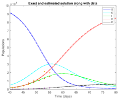
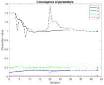
In many problems we are interested in recovering the vector of unknown parameters ${\textstyle {\boldsymbol {\theta }}}$, assuming that we are given the exact initial conditions ${\textstyle \mathbf {x} _{0}}$ and the experimental data ${\textstyle \{{\overline {\mathbf {x} }}_{i}\}_{i=1}^{m}}$ at the corresponding times ${\textstyle t_{i}}$. We consider synthetic experimental noisy data with ${\textstyle noise\_level=0.1}$, where the observable variables are ${\textstyle {\overline {\mathbf {x} }}(t_{i})=(I_{i},R_{i},D_{i})^{T}}$ in the time window ${\textstyle t=40+i}$, ${\textstyle 1\leq i\leq 13}$. Table 2 shows the numerical results obtained with the CG-algorithm (F-R variant) and the BFGS-algorithms, with initial guess ${\textstyle \theta ^{0}=(1.4,0.09,0.2,0.001)^{T}}$ and tolerance ${\textstyle \epsilon =10^{-8}}$ to stop the iterations. The relative error is computed component-wise.

Table. 1 Numerical results with the CG and BFGS algorithms.

Method	CG (F-R variant)	BFGS
${\textstyle {\boldsymbol {\theta }}^{0}}$	$(1.4,0.09,0.2,0.001)$	$(1.4,0.09,0.2,0.001)$
Data time window	$t_{i}=40+i$, ${\textstyle 1\leq i\leq 13}$	$t_{i}=40+i$, ${\textstyle 1\leq i\leq 13}$
$\epsilon$, no. iters.	$\epsilon =10^{-8}$, 168	$\epsilon =10^{-8}$, 14
Computed ${\textstyle {\boldsymbol {\theta }}}$	$(1.0769,0.1425,0.2180,0.0143)$	$(1.0768,0.1426,0.2179,0.0143)$
Relative error	$(0.0769,0.0022,0.0898,4.8e(-5))$	$(0.0768,0.0021,0.0897,0.0001)\quad$

We obtain almost the same numerical value for the computed ${\textstyle {\boldsymbol {\theta }}}$ with both algorithms, the main difference is the number of iterations for each algorithm to achieve convergence to the given tolerance. Overall, the most important feature in this experiment is that the numerical computation is stable and the relative error is smaller than the noise level 0.1 (10%) for each parameter. Figure 2 (left), shows the behaviour of ${\textstyle ||\nabla L({\boldsymbol {\theta }})||}$ (logarithmic scale) and clearly show the faster convergence of the BFGS algorithm. Figure 2 (right) illustrate the convergence of the parameters ${\textstyle {\boldsymbol {\theta }}^{\ell }=\left(\alpha ^{\ell },\beta ^{\ell },\gamma ^{\ell },\mu ^{\ell }\right)^{T}}$. Finally, Figure 3 shows the dynamics of the true solution ${\textstyle \mathbf {x} }$ (continuous lines) and the numerical solution obtained with the computed parameters (dashed lines), along with the noisy data (points). We want to emphasize that the initial value for parameter ${\textstyle \gamma ^{0}=0.2}$ is the exact one, since this a parameter is usually assumed to be known. However the numerical algorithms converge for other initial values, like ${\textstyle \gamma ^{0}=0.1}$ or 0.3 with a similar number of iterations.

Figure 2: Left: graph of $\log \left(\nabla L({\boldsymbol {\theta }})^{\ell }\right)$ against iteration value $\ell$. Right figure: Convergence of ${\boldsymbol {\theta }}^{\ell }=\left(\alpha ^{\ell },\beta ^{\ell },\gamma ^{\ell },\mu ^{\ell }\right)^{T}$ with respect to iteration $\ell$ for CG (continuous lines) and for BFGS (dashed lines).

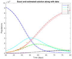
Figure 3: The dynamics of the true solution $\mathbf {x} (t)=\left(S(t),E(t),I(t),R(t),D(t)\right)^{T}$ (continuous lines) and the one obtained with computed ${\boldsymbol {\theta }}$ (dashes lines), along with noisy data for the observable variables $(I_{i},R_{i},D_{i})$ (points).

Example 3: Case when both ${\textstyle \mathbf {x} _{0}}$ and ${\textstyle {\boldsymbol {\theta }}}$ are unknown, ${\textstyle noise\_level=0.1}$.

This problem needs a more careful treatment, we now have to compute nine parameters instead of four and the scale of both unknowns is different: ${\textstyle \mathbf {x} _{0}}$ may have components of the order of ${\textstyle 10^{5}}$ while ${\textstyle {\boldsymbol {\theta }}}$ has components of the order at most ${\textstyle 10^{0}=1}$. The initial guess ${\textstyle {\boldsymbol {\theta }}^{0}}$ to start iterations is the same for both algorithms (CG and BFGS). However, the election of the initial guess ${\textstyle \mathbf {x} _{0}^{0}}$ is more subtle. We first fix the value of ${\textstyle \mathbf {s} _{0}}$ in model (6) with the following formula

$\mathbf {s} _{0}=round(N/{\widehat {N}})\,{\widehat {\mathbf {x} }}_{0}\quad {\hbox{where}}\quad {\widehat {N}}=\sum _{i=1}^{5}{\widehat {x}}_{i\,0},$

(27)

where ${\textstyle {\widehat {\mathbf {x} }}_{0}}$ is obtained from the noisy data at ${\textstyle t=40}$. The adjustment in (3) ensures that the sum of the components of ${\textstyle \mathbf {s} _{0}}$ be equal to ${\textstyle N=10^{5}}$. Observe that ${\textstyle {\widehat {N}}}$ is not guaranteed to be equal to ${\textstyle N}$, because experimental data have inherent noise. Finally, we choose ${\textstyle \mathbf {x} _{0}^{0}=\mathbf {s} _{0}}$ for the CG algorithm and ${\textstyle \mathbf {x} _{0}^{0}={\widehat {\mathbf {x} }}_{0}}$ for the BFGS algorithm. The CG algorithm does not always converge properly with an arbitrary initial value like ${\textstyle \mathbf {x} _{0}^{0}={\widehat {\mathbf {x} }}_{0}}$. Table 2 summarize the numerical results.

Table. 2 Numerical results for computed ${\boldsymbol {\theta }}$ and $\mathbf {x} _{0}$ with CG (P–R) and BFGS algorithms.

Method	CG (P–R variant)	BFGS
${\textstyle {\boldsymbol {\theta }}^{0}}$	$(1.40,0.09,0.20,0.001)$	$(1.40,0.09,0.20,0.001)$
$\mathbf {x} _{0}^{0}$	$(91503,4978,1872,1643,132)$	$(91503,4978,1872,1643,132)$
Data time window	$t_{i}=40+(2i-1)$, ${\textstyle 1\leq i\leq 8}$	$t_{i}=40+(2i-1)$, ${\textstyle 1\leq i\leq 8}$
$\epsilon$, no. iters.	$10^{-5}$, 229	$10^{-6}$, 41
Computed ${\textstyle {\boldsymbol {\theta }}}$	$(1.0075,0.1420,0.2018,0.0134)$	$(1.0077,0.1419,0.2003,0.0132)$
Relative error	$(0.0075,0.0058,0.0090,0.0590)$	$(0.0077,0.0064,0.0016,0.0758)$
Computed ${\textstyle \mathbf {x} _{0}}$	$(91386,4972,1870,1641,132)$	$(91340,4996,1844,1681,139)$
Relative error	$(0.0029,0.0245,0.0654,0.0128,0.0548)$	$(0.0034,0.0294,0.0505,0.0379,0.1148)$

This time the CG algorithm does not admit tolerances smaller than ${\textstyle \epsilon =10^{-5}}$ and also the P-R variant to compute ${\textstyle \beta _{\ell }}$ at step 8 turn out to be more efficient than F-R. We observe that the window time for experimental data is wider but with less data points for both algorithms. The computed ${\textstyle {\boldsymbol {\theta }}}$ obtained with both algorithms is almost the same, but the computed ${\textstyle \mathbf {x} _{0}}$ exhibits more discrepancy. This lack of stability on the estimation of initial conditions from noisy data is already known by the scientific community. In fact, if ${\textstyle \mathbf {f} }$ is Lipschitz continuous with constant ${\textstyle L>0}$, then the sensitivity of the solution of the system (1) with respect to initial conditions is given by ${\textstyle ||\mathbf {x} (t;\mathbf {x} _{0})-\mathbf {x} (t;\mathbf {x} _{0}+\delta \mathbf {x} _{0})||\leq e^{L(t-t_{0})}||\delta \mathbf {x} _{0}||}$.

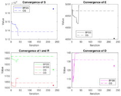
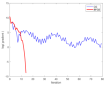
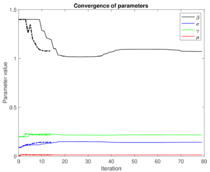
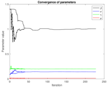
Figures 4 and 5 show information about the convergence of both methods like in the previous example. We have only added in Figure 5 (left) a plot that shows convergence of ${\textstyle \mathbf {x} _{0}^{\ell }}$. The main difference with respect to the previous example is that convergence not only is slower for both methods but also it is not as smooth as before. The convergence curves oscillate a lot more due to a destabilization effect of the unknown initial conditions. However, Figure 5 (right) shows that the overall numerical reproduction of the true solution ${\textstyle \mathbf {x} (t)}$ is much better than in the previous example (all curves are very close to each other).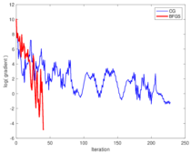

Figure 4: Left: gradient behaviour obtained with the CG (blue line) and the BFGS (red line) algorithms. Right: convergence of ${\boldsymbol {\theta }}$ with CG (continuous lines) and BFGS (dashed lines) algorithms.

Figure 5: Left: convergence of $\mathbf {x} _{0}$ with the CG (dashed lines) and BFGS (continuous lines) algorithms. Right: dynamics of the true solution (continuous lines) and the numerical obtained from $(\mathbf {x} _{0},{\boldsymbol {\theta }})$ computed with CG (dased line) and BFGS (dash-pointed line) algorithms, and noisy data for observable variables $(I_{i},R_{i},D_{i})$ (points)

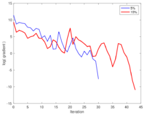
Example 4: This last example includes numerical results obtained with the BFGS algorithm only, but with perturbations ${\textstyle noise\_level=0.05,0.2}$ for the generation of synthetic noisy measurements. Table 4 summarizes the numerical results.

Table. 3 Effect of the noisy data on the numerical results for ${\boldsymbol {\theta }}$ and $\mathbf {x} _{0}$ computed with the BFGS algorithm.

${\textstyle noise\_level}$	$0.05\ (5\%)$	$0.15\ (15\%)$
${\textstyle {\boldsymbol {\theta }}^{0}}$	$(1.40,0.09,0.20,0.001)$	$(1.40,0.09,0.20,0.001)$
$\mathbf {x} _{0}^{0}$	$(91645,4782,1844,1605,124)$	$(90474,5782,1628,987,129)$
Data time window	$t_{i}=40+i$, ${\textstyle 1\leq i\leq 10}$	$t_{i}=40+2i$, ${\textstyle 1\leq i\leq 8}$
$\epsilon$, no. iters.	$10^{-8}$, 30	$10^{-8}$, 43
Computed ${\textstyle {\boldsymbol {\theta }}}$	$(1.0256,0.1356,0.2055,0.0143)$	$(0.9953,0.1385,0.2126,0.0153)$
Relative error	$(0.0256,0.0508,0.0277,0.0004)$	$(0.0047,0.0307,0.0628,0.0705)$
Computed ${\textstyle \mathbf {x} _{0}}$	$(91546,4795,1886,1646,127)$	$(90759,5780,1637,1690,135)$
Relative error	$(0.0011,0.0119,0.0746,0.0160,0.0194)$	$(0.0097,0.1910,0.0675,0.0433,0.0770)$

Comparing these results with those for BFGS in Table 2 we observe that the speed of convergence decreases with increasing ${\textstyle noise\_level}$ for the same tolerance. Also, since the initial guess ${\textstyle \mathbf {x} _{0}^{0}}$ is closer to exact ${\textstyle \mathbf {x} _{0}}$ for the 5% noisy case, then the accuracy of the computed value is better in this case. This sensitivity is not so evident in the calculation of the parameters ${\textstyle {\boldsymbol {\theta }}}$, since the achieved accuracy is comparable. Another feature is that the time window of noisy data is wider the higher the ${\textstyle noise\_level}$ to achieve convergent results. Figures 6 and 7 illustrate the performance of the BFGS algorithm with respect to ${\textstyle noise\_level}$.

Figure 6: Left: plot of $\log(\nabla L(\mathbf {x} _{0},{\boldsymbol {\theta }}))$ against iteration obtained with the BFGS algorithm for 5% noisy data (blue line) and 15% noisy data (red line). Right: convergence of ${\boldsymbol {\theta }}$ for 5% noisy data (continuous lines) and 15% noisy data (dashed lines).

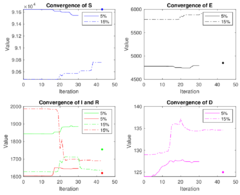
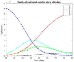
Figure 7: Left: convergence of $\mathbf {x} _{0}$ for 5% noisy data (continuous lines) and 15% noisy data (dashed lines). Right: dynamics of the true solution (continuous lines) and of the numerical solution obtained with 5% noisy data (dashed lines) and 15% noisy data (dash-pointed lines). Here we only show the points with 15% noisy data (see Table 2).

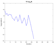
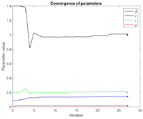
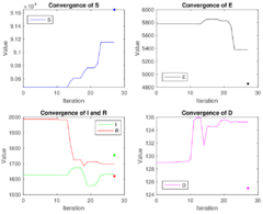
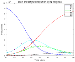
Another way to enhance convergence of the optimization algorithms is adding observable variables. For instance, adding ${\textstyle E}$ as observable variable for the case of 15% noise and using the same numerical parameters in Table 4, the BFGS algorithm converges in 27 iterations for the given tolerance. The best improvement, besides the faster convergence, is the estimation of the initial conditions, as shown in Table 4

Table. 4 Numerical results obtained with the BFGS algorithm, adding $E$ as observable variable.

Parameter	Computed	Relative error
${\textstyle {\boldsymbol {\theta }}}$	$(1.0106,0.1415,0.2131,0.0153)$	$(0.0106,0.0092,0.0657,0.0731)$
$\mathbf {x} _{0}$	$(91154,5381,1632,1698,135)$	$(0.0054,0.1088,0.0704,0.0480,0.0821)$

Figures 6 and 7 show the corresponding improvements.

Figure 8: Left: plot of $\log(\nabla L(\mathbf {x} _{0},{\boldsymbol {\theta }}))$ against iteration obtained with the BFGS algorithm for 15% noisy data and observable variables $(E,I,R,D)$. Right: convergence of ${\boldsymbol {\theta }}$.

Figure 9: Left: convergence of $\mathbf {x} _{0}$ for 15% noisy data and observable variables $(E,I,R,D)$. Right: dynamics of the true solution (continuous lines) and of the numerical solution (dashed lines).

6 Conclusions

We have introduced a deterministic model for fitting observed noisy data into a given dynamical system to find initial conditions and the parameters of the associated system of ordinary differential equations. The classical CG and BFGS optimization algorithms are employed to minimize the quadratic non-linear cost function. It is shown the advantage of using the adjoint equation approach to find the derivatives or gradients. We explain with some detail the implementation of this methods and algorithms with the SEIRD epidemiological model. However, this approach can be equally applied to other problems modelled by ODEs.

Similar numerical results are obtained with both algorithms, CG and BFGS using the same tolerance to achieve a given accuracy, but as expected the BFGS algorithm has better convergence properties and it is more robust. Numerical results show that more experimental data points and more observable variables increase the convergence properties of these algorithms. On the other hand, the higher the noise of the experimental data the slower is the convergence of the optimization algorithms. The main drawback of the proposed methodology is that it is sensitive to the location of noisy data and also to the initial guesses for initial conditions. However, if the algorithms converge properly, then the numerical results obtained are more accurate when ${\textstyle \mathbf {x} _{0}}$ is also estimated along with ${\textstyle {\boldsymbol {\theta }}}$.

For future work, we want to overcome some difficulties or deficiencies that arise with the proposed model and numerical algorithms. First, we must include explicitly into the fitting model (6) the positivity constraint of the unknown parameters, ${\textstyle \mathbf {x} _{0}}$ and ${\textstyle {\boldsymbol {\theta }}}$, specially for those that are relatively small and extend the proposed algorithms accordingly, like in [7]. The inherent instability and difficulty to find the initial conditions may be fixed incorporating the technique of multiple shooting, e.g. [5], [11]. Concerning the efficiency of optimization algorithms, we still need to test the Gauss-Newton method and if necessary its variant, the Levenberg–Marquardt algorithm. Finally, as mentioned before, the line search strategy is crucial for gradient descent algorithms. We may improve the performance of the secant method incorporating bracketing strategies like in [1], or trying the Newton's method as mentioned in remark 7.

Acknowledgements

We want to acknowledge the Department of Mathematics at Universidad Autónoma Metroprolitana – Izatapalapa and to CONACyT for the support for this research work.

BIBLIOGRAPHY

[1] I. K. Argyros, M. A. Hernández-Verón, M. J. Rubio, M. J., On the Convergence of Secant-Like Methods, in Current Trends in Mathematical Analysis and Its Interdisciplinary Applications (2019) 141–183.

[2] J. R. Banga, C. G. Moles, A. A. Alonso, Global optimization of bioprocesses using stochastic and hybrid methods, in: Frontiers in global optimization, Springer (2004) pp. 45–70.

[3] J. Calver and W. Enright, Numerical methods for computing sensitivities for ODEs and DDEs, Numerical Algorithms 74(4) (2017) 1101–1117.

[4] Y. Cao, S. Li,L. Petzold, R. Serban, Adjoint sensitivity analysis for differential algebraic equations: the adjoint DAE system and its numerical solution. SIAM J. Sci. Comput. 3(24) (2003), 1076–1089.

[5] F. Carbonell, Y. Iturria-Medina, J.C. Jimenez, Multiple Shooting-Local Linearization method for the identification of dynamical systems, Communications in Nonlinear Science and Numerical Simulation, 37 C (2016) 292–304.

[6] Calderhead, B., Girolami, M. Estimating Bayes factors via thermodynamic integration and population MCMC Comput. Stat. Data Anal. 53 (12), (2009), 4028–4045.

[7] M. Victoria Chávez, L. Héctor Juárez, Yasmín A. Ríos, Penalization and augmented Lagrangian for OD demand matrix estimation from transit segment counts, Transportmetrica A, Transport Science, 15(2) (2019), 915–943.

[8] J. E. Dennis and Robert B. Schnabel, Numerical Methods for Unconstrained Optimization and Nonlinear Equations, Englewood Cliffs: Prentice-Hall. (1983).

[9] Jorge Nocedal, Stephen J. Wright, Numerical Optimization, New York: Springer, 1999.

[10] I. F. D. Oliveira, R. H. C. Takahashi, An Enhancement of the Bisection Method Average Performance Preserving Minmax Optimality, ACM Transactions on Mathematical Software. 47(1) (2020) 5:1–5:24.

[11] Ozgur Aydogmus, Ali Hakan TOR, A Modified Multiple Shooting Algorithm for Parameter Estimation in ODEs Using Adjoint Sensitivity Analysis, Applied Mathematics and Computation Volume 390(1), (2021) 125644.

[12] Elena L. Piccolomini and Fabiana Zama, Monitoring Italian COVID-19 spread by an adaptive SEIRD model, medRxiv preprint doi: https://doi.org/10.1101/2020.04.03.20049734, April 6, 2020.

[13] Ramsay, J., Hooker, H., Campbell, D., Cao, J. Parameter estimation for differential equations: a generalized smoothing approach. J. R. Stat. Soc. Ser. B 69 (5), (2007) 741–796.

[14] B. Sengupta, K.J. Friston, W.D. Penny, Efficient gradient computation for dynamical models, NeuroImage 98 (2014) 521–527.

[15] Wenyu Sun, Ya-Xiang Yuan, Optimization Theory and Methods:Nonlinear Programming. New York: Springer, 2006.