Performance of stochastic restricted and unrestricted two-parameter estimators in linear mixed models

Abstract

In this article, two parameter estimation using penalized likelihood method in the linear mixed model is proposed. In addition, by considering the stochastic linear restriction for the vector of fixed effects parameters we are introduced the stochastic restricted two parameter estimation. Methods are proposed for estimating variance parameters when unknown. Also, the superiority conditions of the two parameter estimator over the best linear unbiased estimator, and the stochastic restricted two parameter estimator over the stochastic restricted best linear unbiased estimator are obtained under the mean square error matrix sense. Methods are proposed for estimating of the biasing parameters. Finally, a simulation study and a numerical example are given to evaluate the proposed estimators.

Keywords: Linear mixed model, two parameter estimation, stochastic restricted two parameter estimation, matrix mean square error

1. Introduction

Today many datasets lack the assumption of data independence, which is the main presupposition of many statistical models. For example data collected by cluster or hierarchical sampling, lengthwise studies and frequent measurements or in medical research that simultaneously provides data from one or more body members, the assumption of data independence is unacceptable because the data of a cluster, a group, or an individual are interdependent over time [1]. The default requirement for fitting linear models is the assumption of data independence that does not exist so the use of these models although it leads to unbiased estimates but the variance of estimating coefficients is strongly influenced by the default of data independence. In other words if the data are not independent then the standard error and therefore the confidence interval and the result test result will be for non-trust regression coefficients. Therefore in analyzing these data it is necessary to use methods that can consider this dependence. One of the most important ways to solve this problem is linear mixed models which are generalizations of simple linear models that provide the possibility of random and fixed effects with each other. Linear mixed models are used in many fields of physical, biological, medical and social sciences [2-5].

We consider the linear mixed model (LMM) as follows:

${\textstyle y=X\beta +Zu+\epsilon }$ ${\textstyle q=\displaystyle \sum _{i=1}^{b}{q}_{i}}$,

(1)

where ${\textstyle y}$ is an ${\textstyle n\times 1}$ vector of observations, ${\textstyle {\mathit {\boldsymbol {Z}}}=}$$\left[{\mathit {\boldsymbol {Z}}}_{1},\ldots ,{\mathit {\boldsymbol {Z}}}_{b}\right]$ with ${\textstyle {\mathit {\boldsymbol {Z}}}_{i}}$ is an ${\textstyle n\times {q}_{i}}$ design matrix corresponding to the ${\textstyle i}$-th random effects factor and ${\textstyle q}$, ${\textstyle {q}_{i},\,X}$ is an ${\textstyle n\times p}$ observed design matrix for the fixed effects, ${\textstyle \beta }$ is a ${\textstyle p\times 1}$ parameter vector of unknown fixed effects, ${\textstyle {\mathit {\boldsymbol {u}}}={\left[{\mathit {\boldsymbol {u}}}_{1}^{'},\ldots ,{\mathit {\boldsymbol {u}}}_{b}^{'}\right]}^{'}}$ is a ${\textstyle q\times 1}$ unobservable vector of random effects and ${\textstyle {\mathit {\boldsymbol {\epsilon }}}}$ is an ${\textstyle n\times 1}$ unobservable vector of random errors. ${\textstyle u}$ and ${\textstyle \epsilon }$ are independent and have a multivariate normal distribution as

$\left[{\begin{matrix}u\\\epsilon \end{matrix}}\right]\sim \left(\left[{\begin{matrix}0\\0\end{matrix}}\right],{\sigma }^{2}\left[{\begin{matrix}{\mathit {\boldsymbol {G}}}(\zeta )&0\\0&W(\xi )\end{matrix}}\right]\right)$

where ${\textstyle \zeta }$ and ${\textstyle \xi }$ are ${\textstyle {r}_{1}\times 1}$ and ${\textstyle {r}_{2}\times 1}$ vectors of variance parameters corresponding to ${\textstyle u}$ and ${\textstyle \epsilon }$, respectively. Henderson et al. [6-7] introduced the set of equations called mixed model equations, and obtained ${\textstyle {\tilde {\mathit {\boldsymbol {\beta }}}}}$ and ${\textstyle {\tilde {\mathit {\boldsymbol {u}}}}}$ as

${\tilde {\mathit {\boldsymbol {\beta }}}}={\left({\mathit {\boldsymbol {X}}}^{'}{\mathit {\boldsymbol {H}}}^{-1}{\mathit {\boldsymbol {X}}}\right)}^{-1}{\mathit {\boldsymbol {X}}}^{'}{\mathit {\boldsymbol {H}}}^{-1}{\mathit {\boldsymbol {y}}}$

$\left.{\tilde {\mathit {\boldsymbol {u}}}}={\mathit {\boldsymbol {G}}}{\mathit {\boldsymbol {Z}}}^{'}{\mathit {\boldsymbol {H}}}^{-1}({\mathit {\boldsymbol {y}}}-{\mathit {\boldsymbol {X}}}{\tilde {\mathit {\boldsymbol {\beta }}}})\right)$

where ${\textstyle \mathrm {Var} \,({\mathit {\boldsymbol {y}}})={\sigma }^{2}{\mathit {\boldsymbol {H}}}}$ and ${\textstyle {\mathit {\boldsymbol {H}}}=}$${\mathit {\boldsymbol {ZG}}}{\mathit {\boldsymbol {Z}}}^{'}+{\mathit {\boldsymbol {W}}}$. They ${\textstyle {\tilde {\mathit {\boldsymbol {\beta }}}}}$ and ${\textstyle {\tilde {\mathit {\boldsymbol {u}}}}}$ are called the best linear unbiased estimator (BLUE) and the best linear unbiased predictor (BLUP), respectively. One of the most common estimators in linear regression is the ordinary least squares (OLS) estimator, which in the case of multicollinearity may lead to estimates with adverse effects such as high variance [8]. To reduce the effects of multicollinearity. Liu et al. [9-10] proposed the ridge estimator and the Liu estimator respectively, which are the well-known alternatives of the OLS estimator. Yang and Chang [11] obtained the two parameter estimator ${\textstyle {\overset {\mbox{ˆ}}{\mathit {\boldsymbol {\beta }}}}(k,d),}$ “Using the mixed estimation technique introduced by Theil et al. [12-13]. They considered the prior information about ${\textstyle {\mathit {\boldsymbol {\beta }}}}$ in the form of restriction as ${\textstyle (d-}$$k){\overset {\mbox{ˆ}}{\mathit {\boldsymbol {\beta }}}}(k)={\mathit {\boldsymbol {\beta }}}+$${\mathit {\boldsymbol {\epsilon }}}_{0},$ where ${\textstyle k,d}$ and ${\textstyle {\overset {\mbox{ˆ}}{\mathit {\boldsymbol {\beta }}}}(k)}$ are respectively the ridge, Liu parameters and the ridge estimator”.

In ${\textstyle LMM}$, authors such as Gilmour et al. [14], Jiming and Lahiri [15] and Patel and Patel [16], considered a state where the matrix ${\textstyle {X}^{'}{H}^{-1}X}$ is singular. Liu and Hu [10] and Eliot et al. [17] inquired the ridge prediction in LMM. Liu and Hu [10] are obtained ${\textstyle {\tilde {\mathit {\boldsymbol {\beta }}}}(k)}$ and ${\textstyle {\tilde {\mathit {\boldsymbol {u}}}}(k)}$ as

${\tilde {\mathit {\boldsymbol {\beta }}}}(k)={\left({\mathit {\boldsymbol {X}}}^{'}{\mathit {\boldsymbol {H}}}^{-1}{\mathit {\boldsymbol {X}}}+k{\mathit {\boldsymbol {I}}}_{p}\right)}^{-1}{\mathit {\boldsymbol {X}}}{\mathit {\boldsymbol {H}}}^{-1}{\mathit {\boldsymbol {y}}}$

${\tilde {u}}(k)=G{Z}^{'}{H}^{-1}(y-X{\tilde {\beta }}(k))$

where ${\textstyle {\tilde {\mathit {\boldsymbol {\beta }}}}(k)}$ and ${\textstyle {\tilde {\mathit {\boldsymbol {u}}}}(k)}$ are the ridge estimator of ${\textstyle {\mathit {\boldsymbol {\beta }}}}$ and the ridge predictor of ${\textstyle {\mathit {\boldsymbol {u}}},}$ respectively. Özkale and Can [18] gave “an example from kidney failure data” to evaluate ridge estimator in linear mixed model. Kuran and Özkale [19] obtained the mixed and stochastic restricted ridge predictors by using Gilmour approach. They introduced “stochastic linear restriction as ${\textstyle r=}$$R\beta +\Phi$ where ${\textstyle r}$ is an ${\textstyle m\times 1}$ vector, ${\textstyle {\mathit {\boldsymbol {R}}}}$ is an ${\textstyle m\times p}$ known matrix of rank ${\textstyle m\leq p}$ and ${\textstyle \Phi }$ is an ${\textstyle m\times 1}$ random vector that is assumed to be distributed with ${\textstyle E(\Phi )=}$$0$ and ${\textstyle \mathrm {Var} \,(\Phi )={\sigma }^{2}{\mathit {\boldsymbol {V}}}({\mathit {\boldsymbol {v}}}),}$ where ${\textstyle v}$ is ${\textstyle v\times 1}$ vector of variance parameters corresponding to ${\textstyle \Phi .}$ Also ${\textstyle \Phi }$ and ${\textstyle \epsilon }$ are independent”

Then derived the stochastic restricted estimator of ${\textstyle \beta }$ and the stochastic restricted predictor of ${\textstyle {\mathit {\boldsymbol {u}}}}$ respectively, as

${\tilde {\mathit {\boldsymbol {\beta }}}}_{r}={\left({\mathit {\boldsymbol {X}}}^{'}{\mathit {\boldsymbol {H}}}^{-1}{\mathit {\boldsymbol {X}}}+{\mathit {\boldsymbol {R}}}^{'}{\mathit {\boldsymbol {V}}}^{-1}{\mathit {\boldsymbol {R}}}\right)}^{-1}\left({\mathit {\boldsymbol {X}}}^{'}{\mathit {\boldsymbol {H}}}^{-1}{\mathit {\boldsymbol {y}}}+\right.$$\left.{\mathit {\boldsymbol {R}}}^{'}{\mathit {\boldsymbol {V}}}^{-1}{\mathit {\boldsymbol {r}}}\right)$

${\tilde {u}}_{r}=G{Z}^{'}{H}^{-1}\left(y-X{\tilde {\beta }}_{r}\right)$

Furthermore, they obtained the stochastic restricted ridge estimator of ${\textstyle \beta }$ and the stochastic restricted ridge predictor of ${\textstyle {\mathit {\boldsymbol {u}}}}$ respectively, as

${\tilde {\mathit {\boldsymbol {\beta }}}},(k)={\left({\mathit {\boldsymbol {X}}}^{'}{\mathit {\boldsymbol {H}}}^{-1}{\mathit {\boldsymbol {X}}}+{\mathit {\boldsymbol {R}}}^{'}{\mathit {\boldsymbol {V}}}^{-1}{\mathit {\boldsymbol {R}}}+{\mathit {\boldsymbol {H}}}_{p}\right)}^{-1}\left({\mathit {\boldsymbol {X}}}^{'}{\mathit {\boldsymbol {H}}}^{-1}{\mathit {\boldsymbol {y}}}+{\mathit {\boldsymbol {R}}}^{'}{\mathit {\boldsymbol {V}}}^{-1}{\mathit {\boldsymbol {r}}}\right)$

${\tilde {\mathit {\boldsymbol {u}}}}_{r}(k)={\mathit {\boldsymbol {G}}}{\mathit {\boldsymbol {Z}}}^{'}{\mathit {\boldsymbol {H}}}^{-1}\left({\mathit {\boldsymbol {y}}}-{\mathit {\boldsymbol {X}}}{\tilde {\mathit {\boldsymbol {\beta }}}}_{r}(k)\right)$

In this article, we obtain the new two parameter estimations in linear mixed models by taking Yang and Chang’s ideas [11] and considering restriction ${\textstyle (d-}$$k){\tilde {\beta }}(k)=\beta +{\epsilon }_{0}.$ In Section ${\textstyle 2,}$ we follow the idea of Henderson’s mixed model equations to get the two parameter estimator. Then, by setting stochastic linear restrictions ${\textstyle r=}$$R\beta +\Phi$ on the vector of fixed effects parameters, we derive the stochastic restricted two parameter estimation. In Section 3, estimates for the variance parameters are obtained when unknown. In Section 4, under the mean square error matrix (MSEM) sense we offer comparisons of new two parameter estimators. In Section 5, Methods are proposed for estimating of the biasing parameters. In Sections 6 and 7, a simulation study and a real data analysis is given. Finally, summary and some conclusions are given in Section 8.

2. The proposed estimators

Under model (1), we have

$\left[{\begin{matrix}u\\y\end{matrix}}\right]\sim N\left(\left[{\begin{matrix}0\\X{\mathit {\boldsymbol {\beta }}}\end{matrix}}\right],{\sigma }^{2}\left[{\begin{matrix}G&G{Z}^{'}\\ZG&H\end{matrix}}\right]\right)$

and the joint distribution of ${\textstyle u}$ and ${\textstyle y}$ is given by

$h({\mathit {\boldsymbol {y}}},{\mathit {\boldsymbol {u}}})=h({\mathit {\boldsymbol {y}}}\mid {\mathit {\boldsymbol {u}}})h({\mathit {\boldsymbol {u}}})=$${\frac {\mathrm {exp} \,\left\{{\frac {-1}{2{\sigma }^{2}}}\left(({\mathit {\boldsymbol {y}}}-{\mathit {\boldsymbol {X\beta }}}-{\mathit {\boldsymbol {Zu}}}{)}^{'}{\mathit {\boldsymbol {W}}}^{-1}({\mathit {\boldsymbol {y}}}-{\mathit {\boldsymbol {X\beta }}}-{\mathit {\boldsymbol {Zu}}})+{\mathit {\boldsymbol {u}}}^{'}{\mathit {\boldsymbol {G}}}^{-1}{\mathit {\boldsymbol {u}}}\right)\right\}}{{\left.{\left(2\pi {\sigma }^{2}\right)}^{(n+q)/2}{\mathit {\boldsymbol {W}}}\right|}^{1/2}\vert {\mathit {\boldsymbol {G}}}{\vert }^{1/2}}}$

where ${\textstyle G}$ and ${\textstyle W}$ are nonsingular. If the restriction used by Yang and Ghang [11] in linear regression is transferred to linear mixed model, we can produce the two parameter estimator using “penalized term” idea. So by unifying restriction ${\textstyle (d-}$$k){\tilde {\beta }}(k)=\beta +{\epsilon }_{0}$ with model (1) to give

${\textstyle {y}_{\ast }={X}_{\ast }+{Z}_{\ast }u+{\epsilon }_{\ast }}$

(2)

where

${\epsilon }_{0}\sim N\left(0,{I}_{\ast }\right)$

with

${\begin{array}{lll}{I}_{\ast }={\sigma }^{2}{I}_{p},&\quad {y}_{\ast }=\left[{\begin{matrix}y\\(d-k){\tilde {\beta }}(k)\end{matrix}}\right],&\quad {X}_{\ast }=\left[{\begin{matrix}X\\{I}_{p}\end{matrix}}\right],\\{Z}_{\star }=\left[{\begin{matrix}Z\\0\end{matrix}}\right],&\quad {\epsilon }_{\ast }=\left[{\begin{matrix}\epsilon \\{\epsilon }_{0}\end{matrix}}\right],&\quad {W}_{\star }=\left[{\begin{matrix}W&0\\0&{I}_{\star }\end{matrix}}\right]\end{array}}$

Then ${\textstyle u}$ and ${\textstyle {y}_{\ast }}$ are jointly distributed as

$\left[{\begin{matrix}u\\{y}_{\star }\end{matrix}}\right]\sim N\left[\left[{\begin{matrix}0\\{X}_{\star }\end{matrix}}\right]\right],{\sigma }^{2}\left[{\begin{matrix}G&G{Z}_{\star }^{'}\\{Z}_{\star }G&{H}_{\star }\end{matrix}}\right]$

where ${\textstyle {H}_{\star }=Z,G{Z}_{\star }^{'}+{W}_{\star }=\left[{\begin{matrix}H&0\\0&{I}_{\star }\end{matrix}}\right]}$ .The conditional distribution of ${\textstyle {y}_{\ast }}$ given ${\textstyle u}$ is ${\textstyle {y}_{\ast }\mid u\sim N\left(X,\beta +\right.}$$\left.{Z}_{\ast }u,{W}_{\ast }\right)$ and the logarithm joint density of ${\textstyle {y}_{\ast }}$ and ${\textstyle u}$ given by

${\begin{array}{ll}\mathrm {ln} \,f(y,u)&\,=\displaystyle {\frac {-1}{2{\sigma }^{2}}}\left[{\left({y}_{\ast }-{X}_{+}\beta -{Z}_{\ast }u\right)}^{'}{W}_{\ast }^{-1}\left({y}_{\ast }-{X}_{+}\beta -{Z}_{+}u\right)+{u}^{'}{G}^{-1}u\right]\\&\,\,\,-\displaystyle {\frac {n+p+q}{2}}\mathrm {ln} \,\left(2\pi {\sigma }^{2}\right)-\displaystyle {\frac {1}{2}}\mathrm {ln} \,\left|{W}_{\ast }\right|-\displaystyle {\frac {1}{2}}\mathrm {ln} \,\vert G\vert \end{array}}$

The penalized log-likelihood function is obtained by succession ${\textstyle {y}_{\ast },{X}_{\ast },{Z}_{\ast }}$ and ${\textstyle {W}_{+in}}$ ${\textstyle {\left({y}_{\ast }-{X}_{\ast }\beta -{Z}_{\ast }u\right)}^{'}{W}_{\ast }^{-1}\left({y}_{\ast }-\right).}$$\left.{X}_{\ast }\beta -{Z}_{\ast }u\right),$ as follows:

${\begin{array}{ll}\mathrm {ln} \,f(y,u)&=\displaystyle {\frac {-1}{2{\sigma }^{2}}}\left[{y}^{'}{W}^{-1}y+(d-k{)}^{2}{\tilde {\beta }}^{'}(k){\tilde {\beta }}(k)-2{\beta }^{'}{X}^{'}{W}^{-1}y-2(d-k){\tilde {\beta }}^{'}(k)\beta \right.\\&\left.-2{u}^{'}{Z}^{-1}y+2{\beta }^{'}{X}^{'}{W}^{-1}Zu+{\beta }^{'}\left(X{W}^{-1}X+{I}_{p}\right)\beta +{u}^{'}{Z}^{'}{W}^{-1}Zu+{u}^{'}{G}^{-1}u\right]\\&\,-\displaystyle {\frac {n+p+q}{2}}\mathrm {ln} \,\left(2\pi {\sigma }^{2}\right)-\displaystyle {\frac {1}{2}}\mathrm {ln} \,\vert W\vert -\displaystyle {\frac {1}{2}}\mathrm {ln} \,\vert G\vert \end{array}}$

(3)

From Eq. (3), we get the partial derivative with respect to ${\textstyle \beta }$ and ${\textstyle {\mathit {\boldsymbol {u}}},}$ then set the equations to zero and by using ${\textstyle {\tilde {\beta }}(k,d)}$ and ${\textstyle {\tilde {u}}(k,d)}$ to denote the solutions give

$\left({\mathit {\boldsymbol {X}}}^{'}{\mathit {\boldsymbol {W}}}^{-1}{\mathit {\boldsymbol {X}}}+{\mathit {\boldsymbol {I}}}_{p}\right){\tilde {\mathit {\boldsymbol {\beta }}}}\left(k,d\right)+{\mathit {\boldsymbol {X}}}^{'}{\mathit {\boldsymbol {W}}}^{-1}{\mathit {\boldsymbol {Z}}}{\tilde {\mathit {\boldsymbol {u}}}}\left(k,d\right)={\mathit {\boldsymbol {X}}}^{'}{\mathit {\boldsymbol {W}}}^{-1}{\mathit {\boldsymbol {y}}}+\left(d-k\right){\tilde {\mathit {\boldsymbol {\beta }}}}\left(k\right)$

(4)

${\mathit {\boldsymbol {Z}}}^{'}{\mathit {\boldsymbol {W}}}^{-1}{\mathit {\boldsymbol {X}}}{\tilde {\mathit {\boldsymbol {\beta }}}}\left(k,d\right)+\left({\mathit {\boldsymbol {Z}}}^{'}{\mathit {\boldsymbol {W}}}^{-1}{\mathit {\boldsymbol {Z}}}+{\mathit {\boldsymbol {G}}}^{-1}\right){\tilde {\mathit {\boldsymbol {u}}}}\left(k,d\right)={\mathit {\boldsymbol {Z}}}^{'}{\mathit {\boldsymbol {W}}}^{-1}{\mathit {\boldsymbol {y}}}$

(5)

By solving the Eq. (5),${\tilde {u}}(k,d)$ is

${\begin{array}{ll}{\tilde {u}}(k,d)&={\left({\mathit {\boldsymbol {Z}}}^{'}{\mathit {\boldsymbol {W}}}^{-1}{\mathit {\boldsymbol {Z}}}+{\mathit {\boldsymbol {G}}}^{-1}\right)}^{-1}\left({\mathit {\boldsymbol {Z}}}^{'}{\mathit {\boldsymbol {W}}}^{-1}{\mathit {\boldsymbol {y}}}-{\mathit {\boldsymbol {Z}}}^{'}{\mathit {\boldsymbol {W}}}^{-1}{\mathit {\boldsymbol {X}}}{\tilde {\mathit {\boldsymbol {\beta }}}}(k,d)\right)\\&={\left({\mathit {\boldsymbol {Z}}}^{'}{\mathit {\boldsymbol {W}}}^{-1}{\mathit {\boldsymbol {Z}}}+{\mathit {\boldsymbol {G}}}^{-1}\right)}^{-1}{\mathit {\boldsymbol {Z}}}^{'}{\mathit {\boldsymbol {W}}}^{-1}({\mathit {\boldsymbol {y}}}-{\mathit {\boldsymbol {X\beta }}}(k,d))\end{array}}$

(6)

Using ${\textstyle {\tilde {u}}(k,d)}$ into Eq. (4) we get

${\begin{matrix}\left({\mathit {\boldsymbol {X}}}{\mathit {\boldsymbol {W}}}^{-1}{\mathit {\boldsymbol {X}}}+{\mathit {\boldsymbol {I}}}_{p}\right){\tilde {\mathit {\boldsymbol {\beta }}}}(k,d)+{\mathit {\boldsymbol {X}}}{\mathit {\boldsymbol {W}}}^{-1}{\mathit {\boldsymbol {Z}}}{\left({\mathit {\boldsymbol {Z}}}{\mathit {\boldsymbol {W}}}^{-1}{\mathit {\boldsymbol {Z}}}+{\mathit {\boldsymbol {G}}}^{-1}\right)}^{-1}{\mathit {\boldsymbol {Z}}}{\mathit {\boldsymbol {W}}}^{-1}({\mathit {\boldsymbol {y}}}-{\mathit {\boldsymbol {X}}}{\tilde {\mathit {\boldsymbol {\beta }}}}(k,d))\\={\mathit {\boldsymbol {X}}}{\mathit {\boldsymbol {W}}}^{-1}{\mathit {\boldsymbol {y}}}+(d-k){\tilde {\mathit {\boldsymbol {\beta }}}}(k)\end{matrix}}$

(7)

Also using ${\textstyle {H}^{-1}={\left({Z}^{'}GZ+W\right)}^{-1}={W}^{-1}-}$${W}^{-1}Z{\left({Z}^{'}{W}^{-1}Z+{G}^{-1}\right)}^{-1}{Z}^{'}{W}^{-1},$ this equation equals to

${\tilde {\beta }}(k,d)={\left({X}^{'}{H}^{-1}X+{I}_{p}\right)}^{-1}\left({X}^{'}{H}^{-1}y+(d-k){\tilde {\beta }}(k)\right)$

(8)

In Eq. (8), if we put ${\textstyle {\tilde {\mathit {\boldsymbol {\beta }}}}(k)=}$${\left({\mathit {\boldsymbol {X}}}^{'}{\mathit {\boldsymbol {H}}}^{-1}{\mathit {\boldsymbol {X}}}+{\mathit {\boldsymbol {k}}}{\mathit {\boldsymbol {I}}}_{p}\right)}^{-1}{\mathit {\boldsymbol {X}}}^{'}{\mathit {\boldsymbol {H}}}^{-1}{\mathit {\boldsymbol {y}}},{\tilde {\mathit {\boldsymbol {\beta }}}}(k,d)$ is obtained as follows

${\textstyle {\tilde {\beta }}(k,d)=}$${\left({\mathit {\boldsymbol {X}}}^{'}{\mathit {\boldsymbol {H}}}^{-1}{\mathit {\boldsymbol {X}}}+{\mathit {\boldsymbol {I}}}_{p}\right)}^{-1}\left({\mathit {\boldsymbol {X}}}^{'}{\mathit {\boldsymbol {H}}}^{-1}{\mathit {\boldsymbol {X}}}+\right.$$\left.d{\mathit {\boldsymbol {I}}}_{p}\right){\left({\mathit {\boldsymbol {X}}}^{'}{\mathit {\boldsymbol {H}}}^{-1}{\mathit {\boldsymbol {X}}}+k{\mathit {\boldsymbol {I}}}_{p}\right)}^{-1}{\mathit {\boldsymbol {X}}}{\mathit {\boldsymbol {H}}}^{-1}{\mathit {\boldsymbol {y}}}$

(9)

Due to ${\textstyle \left({Z}^{'}{W}^{-1}Z+{G}^{-1}\right)G{Z}^{'}={Z}^{'}{W}^{-1}ZG{Z}^{'}+{Z}^{'}={Z}^{'}{W}^{-1}\left(ZG{Z}^{'}+W\right)={Z}^{'}{W}^{-1}H,}$ we get

${\textstyle {\left({\mathit {\boldsymbol {Z}}}^{'}{\mathit {\boldsymbol {W}}}^{-1}{\mathit {\boldsymbol {Z}}}+{\mathit {\boldsymbol {G}}}^{-1}\right)}^{-1}{\mathit {\boldsymbol {G}}}^{'}{\mathit {\boldsymbol {W}}}^{-1}=}$${\mathit {\boldsymbol {G}}}{\mathit {\boldsymbol {Z}}}^{'}{\mathit {\boldsymbol {H}}}^{-1}$

(10)

Using Eq. (10), ${\textstyle {\tilde {u}}(k,d)}$ equals to ${\textstyle {\tilde {u}}(k,d)=GZ{H}^{-1}(y-X{\tilde {\beta }}(k,d))}$.

In section, we obtain the stochastic restricted two parameter estimation. For this, the stochastic Linear restrictions ${\textstyle r=R\beta +\Phi }$ can be unified to model (1) and the restriction ${\textstyle (d-k){\tilde {\beta }},(k)=\beta +{\epsilon }_{0}}$ to give

${\textstyle {\mathit {\boldsymbol {y}}}_{{r}^{\star }}={\mathit {\boldsymbol {X}}}_{{r}^{\star }}{\mathit {\boldsymbol {\beta }}}+{\mathit {\boldsymbol {Z}}}_{r}{\mathit {\boldsymbol {u}}}+{\mathit {\boldsymbol {\epsilon }}}_{\ast ,}}$

(11)

where

${y}_{{r}^{\ast }}=\left[{\begin{matrix}y\\(d-k){\tilde {\beta }}_{r}(k)\\r\end{matrix}}\right],\quad {X}_{{r}^{\ast }}=\left[{\begin{matrix}X\\{I}_{p}\\R\end{matrix}}\right],\quad {Z}_{{r}^{\ast }}=\left[{\begin{matrix}Z\\0\\0\end{matrix}}\right],\quad {\epsilon }_{{r}^{\ast }}=\left[{\begin{matrix}\epsilon \\{\epsilon }_{0}\\\Phi \end{matrix}}\right],\quad {W}_{{r}^{\star }}=\left[{\begin{matrix}W&0&0\\0&{I}_{\ast }&0\\0&0&V\end{matrix}}\right]$

Then, the conditional distribution of ${\textstyle {y}_{\ast }}$ given ${\textstyle {\mathit {\boldsymbol {u}}}}$ is ${\textstyle {\mathit {\boldsymbol {y}}}_{{r}^{\ast }}\mid {\mathit {\boldsymbol {u}}}\sim {\mathit {\boldsymbol {N}}}\left({\mathit {\boldsymbol {X}}}_{{r}^{\ast }}{\mathit {\boldsymbol {\beta }}}+{\mathit {\boldsymbol {Z}}}_{{r}^{\ast }}{\mathit {\boldsymbol {u}}},{\mathit {\boldsymbol {W}}}_{{r}^{\ast }}\right)}$ and the logarithm joint density of ${\textstyle {y}_{r}}$ and ${\textstyle u}$ given by

${\begin{array}{ll}\mathrm {ln} \,g({\mathit {\boldsymbol {y}}},{\mathit {\boldsymbol {u}}})=&\displaystyle {\frac {-1}{2{\sigma }^{2}}}\left[{\left({\mathit {\boldsymbol {y}}}_{{r}^{\ast }}-{\mathit {\boldsymbol {X}}}_{{r}^{\ast }}{\mathit {\boldsymbol {\beta }}}-{\mathit {\boldsymbol {Z}}}_{{r}^{\ast }}{\mathit {\boldsymbol {u}}}\right)}^{'}{\mathit {\boldsymbol {W}}}_{{p}^{\ast }}^{-1}\left({\mathit {\boldsymbol {y}}}_{{r}^{\ast }}-{\mathit {\boldsymbol {X}}}_{{r}^{\ast }}{\mathit {\boldsymbol {\beta }}}-{\mathit {\boldsymbol {Z}}}_{{r}^{\ast }}{\mathit {\boldsymbol {u}}}\right)+{\mathit {\boldsymbol {u}}}^{'}{\mathit {\boldsymbol {G}}}^{-1}{\mathit {\boldsymbol {u}}}\right]\\&-\displaystyle {\frac {n+m+p+q}{2}}\mathrm {ln} \,\left(2\pi {\sigma }^{2}\right)-\displaystyle {\frac {1}{2}}\mathrm {ln} \,\left|{\mathit {\boldsymbol {W}}}_{r\ast }\right|-\displaystyle {\frac {1}{2}}\mathrm {ln} \,\vert {\mathit {\boldsymbol {G}}}\vert \end{array}}$

Substituting ${\textstyle {y}_{r},{X}_{{r}^{\ast }}{Z}_{{r}^{\ast }}}$ and ${\textstyle {W}_{{r}^{+}}}$ to ${\textstyle {\left({y}_{{r}^{\ast }}-{X}_{{r}^{\ast }}\beta -{Z}_{{r}^{\ast }}u\right)}^{'}{W}_{{\gamma }^{\ast }}^{-1}\left({y}_{{r}^{\ast }}-{X}_{{r}^{\ast }}\beta -{Z}_{{r}^{\ast }}u\right)}$, the penalized log-likelihood function is obtained as follows:

${\begin{matrix}\mathrm {ln} \,g(y,u)=\displaystyle {\frac {-1}{2{\sigma }^{2}}}\left[{y}^{'}{W}^{-1}y+(d-k{)}^{2}{\tilde {\beta }}_{r}^{'}(k){\tilde {\beta }}_{r}(k)+{r}^{'}{V}^{-1}r-2{\beta }^{'}X{W}^{-1}y-2(d-k){\tilde {\beta }}_{r}^{'}(k)\beta \right.\\-2{u}^{'}{Z}^{'}{W}^{-1}y-2{\beta }^{'}{R}^{'}{V}^{-1}r+\beta {R}^{'}{V}^{-1}R\beta +\beta \left(X{W}^{-1}X+{I}_{p}\right)\beta +2{u}^{'}Z{W}^{-1}X\beta \\\left.+{u}^{'}Z{W}^{-1}Zu+{u}^{'}{G}^{-1}u\right]-\displaystyle {\frac {n+m+p+q}{2}}\mathrm {ln} \,\left(2\pi {\sigma }^{2}\right)-\displaystyle {\frac {1}{2}}\mathrm {ln} \,{W}_{{r}^{\star }}\left|-\displaystyle {\frac {1}{2}}ln\right|G\mid \end{matrix}}$

(12)

From Eq. (12), we get the partial derivative with respect to ${\textstyle \beta }$ and ${\textstyle {\mathit {\boldsymbol {u}}},}$ then set the equations to zero and by using ${\textstyle {\tilde {\beta }}_{r}(k,d)}$ and ${\textstyle {\tilde {u}}_{r}(k,d)}$ to denote the solutions give

$\left({\mathit {\boldsymbol {X}}}^{'}{\mathit {\boldsymbol {W}}}^{-1}{\mathit {\boldsymbol {X}}}+{\mathit {\boldsymbol {R}}}^{'}{\mathit {\boldsymbol {V}}}^{-1}{\mathit {\boldsymbol {R}}}+{\mathit {\boldsymbol {I}}}_{p}\right){\tilde {\mathit {\boldsymbol {\beta }}}}_{r}(k,d)+{\mathit {\boldsymbol {X}}}{\mathit {\boldsymbol {W}}}^{-1}{\mathit {\boldsymbol {Z}}}{\tilde {\mathit {\boldsymbol {u}}}}_{r}(k,d)={\mathit {\boldsymbol {X}}}{\mathit {\boldsymbol {W}}}^{-1}{\mathit {\boldsymbol {y}}}+(d-k){\tilde {\mathit {\boldsymbol {\beta }}}},(k)+{\mathit {\boldsymbol {R}}}^{'}{\mathit {\boldsymbol {V}}}^{-1}{\mathit {\boldsymbol {r}}}$

(13)

${\mathit {\boldsymbol {Z}}}^{'}{\mathit {\boldsymbol {W}}}^{-1}{\mathit {\boldsymbol {X}}}{\tilde {\mathit {\boldsymbol {\beta }}}}_{r}\left(k,d\right)+\left({\mathit {\boldsymbol {Z}}}{\mathit {\boldsymbol {W}}}^{-1}{\mathit {\boldsymbol {Z}}}+{\mathit {\boldsymbol {G}}}^{-1}\right){\tilde {\mathit {\boldsymbol {u}}}}_{r}\left(k,d\right)={\mathit {\boldsymbol {Z}}}{\mathit {\boldsymbol {W}}}^{-1}{\mathit {\boldsymbol {y}}}$

(14)

By solving these equations similar to Eqs. (4) and (5), the following results are obtained

${\begin{array}{ll}{\tilde {\mathit {\boldsymbol {\beta }}}}_{r}\left(k,d\right)&={\left({\mathit {\boldsymbol {X}}}{\mathit {\boldsymbol {H}}}^{-1}{\mathit {\boldsymbol {X}}}+{\mathit {\boldsymbol {R}}}^{'}{\mathit {\boldsymbol {V}}}^{-1}{\mathit {\boldsymbol {R}}}+{\mathit {\boldsymbol {I}}}_{p}\right)}^{-1}\left({\mathit {\boldsymbol {X}}}{\mathit {\boldsymbol {H}}}^{-1}{\mathit {\boldsymbol {X}}}+{\mathit {\boldsymbol {R}}}^{'}{\mathit {\boldsymbol {V}}}^{-1}{\mathit {\boldsymbol {R}}}+d{\mathit {\boldsymbol {I}}}_{p}\right)\\&\times {\left({\mathit {\boldsymbol {X}}}{\mathit {\boldsymbol {H}}}^{-1}{\mathit {\boldsymbol {X}}}+{\mathit {\boldsymbol {R}}}^{'}{\mathit {\boldsymbol {V}}}^{-1}{\mathit {\boldsymbol {R}}}+k{\mathit {\boldsymbol {I}}}_{p}\right)}^{-1}\left({\mathit {\boldsymbol {X}}}{\mathit {\boldsymbol {H}}}^{-1}{\mathit {\boldsymbol {y}}}+{\mathit {\boldsymbol {R}}}^{\boldsymbol {'}}{\mathit {\boldsymbol {V}}}^{-1}{\mathit {\boldsymbol {r}}}\right)\end{array}}$

(15)

${\tilde {\mathit {\boldsymbol {u}}}}_{r}\left(k,d\right)={\mathit {\boldsymbol {G}}}{\mathit {\boldsymbol {Z}}}^{'}{\mathit {\boldsymbol {H}}}^{-1}\left({\mathit {\boldsymbol {y}}}-{\mathit {\boldsymbol {X}}}{\tilde {\mathit {\boldsymbol {\beta }}}}_{r}\left(k,d\right)\right)$

(16)

3. Estimation of variance parameters

In linear mixed models, the variance parameter within ${\textstyle G}$ and ${\textstyle W}$ are often unknown that several methods have been proposed by [16,20-22] to estimate them. In this section, we estimate the variance parameters using the ML method. The marginal distribution of ${\textstyle {y}_{\ast }}$ is ${\textstyle N\left({\mathit {\boldsymbol {X}}}\cdot {\mathit {\boldsymbol {\beta }}},{\sigma }^{2}{\mathit {\boldsymbol {H}}}_{\ast }\right)}$, therefore we can write the marginal log-likelihood function of ${\textstyle {\mathit {\boldsymbol {y}}}}$

${l}_{ML}\left({\mathit {\boldsymbol {\beta }}},{\mathit {\boldsymbol {\phi }}},{\mathit {\boldsymbol {y}}}_{\ast }\right)=$$\displaystyle {\frac {-1}{2{\sigma }^{2}}}\left\{{\left({\mathit {\boldsymbol {y}}}_{\ast }-{\mathit {\boldsymbol {X}}}_{\ast }{\mathit {\boldsymbol {\beta }}}\right)}^{'}{\mathit {\boldsymbol {H}}}_{\ast }^{-1}\left({\mathit {\boldsymbol {y}}}_{\ast }-\right.\right.$$\left.\left.{\mathit {\boldsymbol {X}}}_{\ast }{\mathit {\boldsymbol {\beta }}}\right)\right\}-$${\frac {n+p}{2}}\mathrm {ln} \,\left(2\pi {\mathit {\boldsymbol {\sigma }}}^{2}\right)-$$\displaystyle {\frac {1}{2}}\mathrm {ln} \,\left|{\mathit {\boldsymbol {H}}}_{\ast }\right|$

(17)

where ${\textstyle \phi ={\left({\mathit {\boldsymbol {K}}}^{'},{\sigma }^{2}\right)}^{'},{\mathit {\boldsymbol {k}}}={\left({\zeta }^{'},{\xi }^{'}\right)}^{'}}$ and ${\textstyle \left({r}_{1}+{r}_{2}+1\right)\times 1}$ and ${\textstyle \left({r}_{1}+{r}_{2}\right)\times 1}$ are vectors of unknown parameters, respectively. Differentiating the Eq. (17) with respect to ${\textstyle \beta ,{\sigma }^{2}}$ and ${\textstyle {\kappa }_{j}=}$$1,\ldots ,{r}_{1}+{r}_{2}$ the partial derivatives is obtained as

$\displaystyle {\frac {\partial {l}_{ML}\left({\mathit {\boldsymbol {\beta }}},{\mathit {\boldsymbol {\phi }}};{\mathit {\boldsymbol {y}}}_{\ast }\right)}{\partial {\mathit {\boldsymbol {\beta }}}}}=$$\displaystyle {\frac {-1}{{\sigma }^{2}}}\left({\mathit {\boldsymbol {X}}}_{\ast }^{'}{\mathit {\boldsymbol {H}}}_{\ast }^{-1}{\mathit {\boldsymbol {X}}}_{\ast }{\mathit {\boldsymbol {\beta }}}-\right.$$\left.{\mathit {\boldsymbol {X}}}_{\ast }^{'}{\mathit {\boldsymbol {H}}}_{\ast }^{-1}{\mathit {\boldsymbol {y}}}_{\ast }\right),$

(18)

$\displaystyle {\frac {\partial {l}_{ML}\left({\mathit {\boldsymbol {\beta }}},{\mathit {\boldsymbol {\phi }}};{\mathit {\boldsymbol {y}}}_{\ast }\right)}{\partial {\sigma }^{2}}}=$$\displaystyle {\frac {-(n+p)}{2{\sigma }^{2}}}+\displaystyle {\frac {{\left({\mathit {\boldsymbol {y}}}_{\ast }-{\mathit {\boldsymbol {X}}}\cdot {\mathit {\boldsymbol {\beta }}}\right)}^{'}{\mathit {\boldsymbol {H}}}_{\cdot }^{-1}\left({\mathit {\boldsymbol {y}}}_{\ast }-{\mathit {\boldsymbol {X}}}\cdot {\mathit {\boldsymbol {\beta }}}\right)}{2{\sigma }^{4}}},$

(19)

$\displaystyle {\frac {\partial {l}_{ML}\left({\mathit {\boldsymbol {\beta }}},{\mathit {\boldsymbol {\phi }}};{\mathit {\boldsymbol {y}}}_{\ast }\right)}{\partial {\kappa }_{i}}}=$$\displaystyle {\frac {-1}{2}}\mathrm {tr} \,\left({\mathit {\boldsymbol {H}}}_{\ast }^{-1}{\dot {\mathit {\boldsymbol {H}}}}_{{\ast }_{j}}\right)+$$\displaystyle {\frac {{\left({\mathit {\boldsymbol {y}}}_{\ast }-{\mathit {\boldsymbol {X}}}_{\ast }{\mathit {\boldsymbol {\beta }}}\right)}^{'}{\mathit {\boldsymbol {H}}}_{\ast }^{-1}{\dot {\mathit {\boldsymbol {H}}}}_{\ast }{\mathit {\boldsymbol {H}}}_{\ast }^{-1}\left({\mathit {\boldsymbol {y}}}_{\ast }-{\mathit {\boldsymbol {X}}}\cdot {\mathit {\boldsymbol {\beta }}}\right)}{2{\sigma }^{2}}}$

(20)

where ${\textstyle {\dot {H}}_{\ast j}=\partial {H}_{\ast }/\partial {\kappa }_{j}}$. Setting Eqs. (18)-(20) equal to zero and using ${\textstyle {\tilde {\beta }}(k,d),{\tilde {\sigma }}^{2}(k,d)}$ and ${\textstyle {\tilde {H}}}$ and instead of ${\textstyle {\mathit {\boldsymbol {\beta }}},{\sigma }^{2}}$ and ${\textstyle {\mathit {\boldsymbol {H}}}}$ gives

$\&X{\tilde {H}}_{\ast }^{-1}X,{\tilde {\beta }}(k,d)={X}^{'}{\tilde {H}}_{\ast }^{-1}{y}_{\star }$

(21)

$(n+p){\tilde {\sigma }}^{2}(k,d)={\left({y}_{\star }-{X}_{\ast }{\tilde {\beta }}\left(k,d\right)\right)}^{'}{\tilde {H}}_{\ast }^{-1}\left({y}_{\star }-{X}_{\star }{\tilde {\beta }}\left(k,d\right)\right)$

(22)

$(\mathrm {tr} \,\left({\tilde {H}}_{\ast }^{-1}{\tilde {H}}_{\ast j}\right)=\displaystyle {\frac {{\left({y}_{\star }-{X}_{\ast }{\tilde {\beta }}\left(k,d\right)\right)}^{'}{\tilde {H}}_{\ast }^{-1}{\tilde {H}}_{\ast j}{\tilde {H}}_{\ast }^{-1}\left({y}_{\star }-{X}_{\star }{\tilde {\beta }}\left(k,d\right)\right)}{{\tilde {\sigma }}^{2}\left(k,d\right)}}$

(23)

Solving Eqs. (21) and (23) yields the estimators

${\begin{array}{ll}{\tilde {\mathit {\boldsymbol {\beta }}}}(k,d)&={\left({\mathit {\boldsymbol {X}}}_{\ast }^{'}{\tilde {\mathit {\boldsymbol {H}}}}_{\ast }^{-1}{\mathit {\boldsymbol {X}}}_{\ast }\right)}^{-1}{\mathit {\boldsymbol {X}}}_{\ast }^{'}{\tilde {\mathit {\boldsymbol {H}}}}_{\ast }^{-1}{\mathit {\boldsymbol {y}}}_{\ast }\\&={\left({\mathit {\boldsymbol {X}}}^{'}{\tilde {\mathit {\boldsymbol {H}}}}^{-1}{\mathit {\boldsymbol {X}}}+{\mathit {\boldsymbol {I}}}_{p}\right)}^{-1}\left({\mathit {\boldsymbol {X}}}^{'}{\tilde {\mathit {\boldsymbol {H}}}}^{-1}{\mathit {\boldsymbol {X}}}+d{\mathit {\boldsymbol {I}}}_{p}\right){\left({\mathit {\boldsymbol {X}}}^{'}{\tilde {\mathit {\boldsymbol {H}}}}^{-1}{\mathit {\boldsymbol {X}}}+{\mathit {\boldsymbol {k}}}{\mathit {\boldsymbol {I}}}_{p}\right)}^{-1}{\mathit {\boldsymbol {X}}}^{'}{\tilde {\mathit {\boldsymbol {H}}}}^{-1}{\mathit {\boldsymbol {y}}}\end{array}}$

(24)

${\begin{array}{ll}{\tilde {\sigma }}^{2}(k,d)&=\displaystyle {\frac {1}{(n+p)}}{\left({\mathit {\boldsymbol {y}}}_{\ast }-{\mathit {\boldsymbol {X}}}_{\ast }{\tilde {\mathit {\boldsymbol {\beta }}}}(k,d)\right)}^{'}{\tilde {\mathit {\boldsymbol {H}}}}_{\cdot }^{-1}\left({\mathit {\boldsymbol {y}}}_{\ast }-{\mathit {\boldsymbol {X}}}_{\ast }{\tilde {\mathit {\boldsymbol {\beta }}}}(k,d)\right)\\&=\displaystyle {\frac {1}{(n+p)}}\left\{({\mathit {\boldsymbol {y}}}-{\mathit {\boldsymbol {X}}}{\tilde {\mathit {\boldsymbol {\beta }}}}(k,d){)}^{'}{\tilde {\mathit {\boldsymbol {H}}}}^{-1}({\mathit {\boldsymbol {y}}}-{\mathit {\boldsymbol {X}}}{\tilde {\mathit {\boldsymbol {\beta }}}}(k,d))\right.\\&\,\,+\left.({\tilde {\mathit {\boldsymbol {\beta }}}}(k,d)-(d-k){\tilde {\mathit {\boldsymbol {\beta }}}}(k){)}^{'}({\tilde {\mathit {\boldsymbol {\beta }}}}(k,d)-(d-k){\tilde {\mathit {\boldsymbol {\beta }}}}(k))\right\}\end{array}}$

(25)

Eq. (23) depends on ${\textstyle {\tilde {\mathit {\boldsymbol {\beta }}}}(k,d)}$ and ${\textstyle {\tilde {\sigma }}^{2}(k,d),}$ so iterative procedures must be used to solve ${\textstyle {K}_{j}}$'s. In the statistical literature, there are four iterative procedures to estimates variance parameters, which include: "Newton-Raphson (NR), Expectation Maximization algorithm (EM), Fisher Scoring (FS) and the Average Information (AI) algorithms". See [22] for details of these procedures. Note that in the stochastic restricted two parameter methods, the ML estimators is obtained similar Eqs. (21),(22) and (23).

4. Comparison of estimators

In this section, we compare the estimator ${\textstyle {\tilde {\mathit {\boldsymbol {\beta }}}}(k,d)}$ with ${\textstyle {\tilde {\mathit {\boldsymbol {\beta }}}}}$ and the estimator ${\textstyle {\tilde {\mathit {\boldsymbol {\beta }}}}_{r}(k,d)}$ with ${\textstyle {\tilde {\mathit {\boldsymbol {\beta }}}}_{r}}$ using the mean squares error matrix (MSEM) sense. The estimator ${\textstyle {\tilde {\mathit {\boldsymbol {\beta }}}}_{2}}$ is superior to ${\textstyle {\tilde {\mathit {\boldsymbol {\beta }}}}_{1}}$ with respect to the MSEM sense, if and only if ${\textstyle \Delta \left({\tilde {\beta }}_{1},{\tilde {\beta }}_{2}\right)=}$$MSEM\left({\tilde {\beta }}_{1}\right)-MSEM\left({\tilde {\beta }}_{2}\right)>0,$ that is, ${\textstyle \Delta \left({\tilde {\beta }}_{1},{\tilde {\beta }}_{2}\right)}$ is a positive definite (pd) matrix. The mean-square error matrix for the estimator ${\textstyle {\tilde {\mathit {\boldsymbol {\beta }}}}(k,d)}$ is given as

$\mathrm {MSEM} \,({\tilde {\mathit {\boldsymbol {\beta }}}}(k,d),{\mathit {\boldsymbol {\beta }}})=\mathrm {Var} \,({\tilde {\mathit {\boldsymbol {\beta }}}}(k,d))+\mathrm {bias} \,({\tilde {\mathit {\boldsymbol {\beta }}}}(k,d))\mathrm {bias} \,({\tilde {\mathit {\boldsymbol {\beta }}}}(k,d){)}^{'}$

The variance matrix of ${\textstyle {\tilde {\beta }}(k,d)}$ is

$V~ar~({\tilde {\beta }}(k,d))={\sigma }^{2}{T}_{1}{X}^{'}{H}^{-1}X{T}_{1}^{'}$

where ${\textstyle {T}_{1}={\left({X}^{'}{H}^{-1}X+{I}_{p}\right)}^{-1}\left({X}^{'}{H}^{-1}X+\right.}$$\left.d{I}_{p}\right){\left({X}^{'}{H}^{-1}X+k{I}_{p}\right)}^{-1}.$ The bias ${\textstyle ({\tilde {\beta }}(k,d))}$ is given as

bias $({\tilde {\beta }}(k,d))=E({\tilde {\beta }}(k,d)-\beta )=-{\left({\mathit {\boldsymbol {X}}}{\mathit {\boldsymbol {H}}}^{-1}{\mathit {\boldsymbol {X}}}+{\mathit {\boldsymbol {I}}}_{p}\right)}^{-1}{\left({\mathit {\boldsymbol {X}}}{\mathit {\boldsymbol {H}}}^{-1}{\mathit {\boldsymbol {X}}}+k{\mathit {\boldsymbol {I}}}_{p}\right)}^{-1}\left((k+1-\right.$$\left.d){\mathit {\boldsymbol {X}}}{\mathit {\boldsymbol {H}}}^{-1}{\mathit {\boldsymbol {X}}}+\right.$$\left.k{\mathit {\boldsymbol {I}}}_{p}\right){\mathit {\boldsymbol {\beta }}}$

The mean-square error matrix for the estimator ${\textstyle {\tilde {\beta }}_{r}(k,d)}$ is given as

$\mathrm {MSEM} \,\left({\tilde {\mathit {\boldsymbol {\beta }}}}_{r}(k,d),{\mathit {\boldsymbol {\beta }}}\right)=$${\sigma }^{2}{\mathit {\boldsymbol {T}}}_{2}\left({\mathit {\boldsymbol {X}}}^{'}{\mathit {\boldsymbol {H}}}^{-1}{\mathit {\boldsymbol {X}}}+\right.$$\left.{\mathit {\boldsymbol {R}}}^{'}{\mathit {\boldsymbol {V}}}^{-1}{\mathit {\boldsymbol {R}}}\right){\mathit {\boldsymbol {T}}}_{2}^{'}+\mathrm {bias} \,\left({\mathit {\boldsymbol {\beta }}}_{r}(k,d)\right)\mathrm {bias} \,{\left({\mathit {\boldsymbol {\beta }}}_{r}(k,d)\right)}^{'}$

where

${\mathit {\boldsymbol {T}}}_{2}={\left({\mathit {\boldsymbol {X}}}^{'}{\mathit {\boldsymbol {H}}}^{-1}{\mathit {\boldsymbol {X}}}+{\mathit {\boldsymbol {R}}}^{'}{\mathit {\boldsymbol {V}}}^{-1}{\mathit {\boldsymbol {R}}}+{\mathit {\boldsymbol {I}}}_{p}\right)}^{-1}\left({\mathit {\boldsymbol {X}}}^{'}{\mathit {\boldsymbol {H}}}^{-1}{\mathit {\boldsymbol {X}}}+\right.$$\left.{\mathit {\boldsymbol {R}}}^{'}{\mathit {\boldsymbol {V}}}^{-1}{\mathit {\boldsymbol {R}}}+\right.$$\left.d{\mathit {\boldsymbol {I}}}_{p}\right){\left({\mathit {\boldsymbol {X}}}{\mathit {\boldsymbol {H}}}^{-1}{\mathit {\boldsymbol {X}}}+{\mathit {\boldsymbol {R}}}^{\boldsymbol {'}}{\mathit {\boldsymbol {V}}}^{-1}{\mathit {\boldsymbol {R}}}+{\mathit {\boldsymbol {k}}}{\mathit {\boldsymbol {I}}}_{p}\right)}^{-1}$

and

${\begin{array}{ll}{\rm {bias}}\,\left({\tilde {\mathit {\boldsymbol {\beta }}}}_{r}(k,d)\right)&=-{\left({\mathit {\boldsymbol {X}}}{\mathit {\boldsymbol {H}}}^{-1}{\mathit {\boldsymbol {X}}}+{\mathit {\boldsymbol {R}}}^{'}{\mathit {\boldsymbol {V}}}^{-1}{\mathit {\boldsymbol {R}}}+{\mathit {\boldsymbol {I}}}_{p}\right)}^{-1}{\left({\mathit {\boldsymbol {X}}}{\mathit {\boldsymbol {H}}}^{-1}{\mathit {\boldsymbol {X}}}+{\mathit {\boldsymbol {R}}}^{'}{\mathit {\boldsymbol {V}}}^{-1}{\mathit {\boldsymbol {R}}}+k{\mathit {\boldsymbol {I}}}_{p}\right)}^{-1}\\&\times \left((k+1-d)\left({\mathit {\boldsymbol {X}}}{\mathit {\boldsymbol {H}}}^{-1}{\mathit {\boldsymbol {X}}}+{\mathit {\boldsymbol {R}}}^{'}{\mathit {\boldsymbol {V}}}^{-1}{\mathit {\boldsymbol {R}}}\right)+k{\mathit {\boldsymbol {I}}}_{p}\right){\mathit {\boldsymbol {\beta }}}\end{array}}$

4.1 Comparison the Estimator β̃(k,d) with β̃

The ${\textstyle MSEM}$ of ${\textstyle {\tilde {\mathit {\boldsymbol {\beta }}}}}$ is ${\textstyle \mathrm {MSEM} \,({\tilde {\mathit {\boldsymbol {\beta }}}})=}$${\sigma }^{2}{\mathit {\boldsymbol {A}}}^{-1},$ where ${\textstyle {\mathit {\boldsymbol {A}}}_{1}=}$$\left({\mathit {\boldsymbol {X}}}{\mathit {\boldsymbol {H}}}^{-1}{\mathit {\boldsymbol {X}}}\right),$ and the ${\textstyle MSEM}$ of ${\textstyle {\tilde {\mathit {\boldsymbol {\beta }}}}(k,d)}$ is

$\mathrm {MSEM} \,({\tilde {\mathit {\boldsymbol {\beta }}}}(k,d))={\sigma }^{2}{\mathit {\boldsymbol {T}}}_{1}{\mathit {\boldsymbol {A}}}_{1}{\mathit {\boldsymbol {T}}}_{1}^{'}+$$\left({\mathit {\boldsymbol {T}}}_{1}{\mathit {\boldsymbol {A}}}_{1}-{\mathit {\boldsymbol {I}}}_{p}\right)\beta {\mathit {\boldsymbol {\beta }}}^{'}{\left({\mathit {\boldsymbol {T}}}_{1}{\mathit {\boldsymbol {A}}}_{1}-{\mathit {\boldsymbol {I}}}_{p}\right)}^{'}$

The estimator ${\textstyle {\tilde {\beta }}(k,d)}$ is superior to the estimator ${\textstyle {\tilde {\beta }}}$ under the MSEM sense, if and only if ${\textstyle \mathrm {MSEM} \,({\tilde {\mathit {\boldsymbol {\beta }}}})-\mathrm {MSEM} \,({\tilde {\mathit {\boldsymbol {\beta }}}}(k,d))>0}$ then

${\Delta }_{1}=MSEM({\tilde {\beta }})-MSEM({\tilde {\beta }}(k,d))={\sigma }^{2}\left({A}_{1}^{-1}-\right.$$\left.{T}_{1}{A}_{1}{T}_{1}\right)-\left({T}_{1}{A}_{1}-{I}_{p}\right)\beta \beta {\left({T}_{1}{A}_{1}-{I}_{p}\right)}^{'}>0$

According to Farebrother ${\textstyle (1976),}$ if ${\textstyle {\sigma }^{2}\left({A}_{1}^{-1}-\right.}$$\left.{T}_{1}{A}_{1}{T}_{1}\right)>0,$ then the necessary and sufficient condition for ${\textstyle {\tilde {\mathit {\boldsymbol {\beta }}}}(k,d)}$ to be superior to ${\textstyle {\tilde {\mathit {\boldsymbol {\beta }}}}}$ is ${\textstyle {\mathit {\boldsymbol {\beta }}}^{'}{\left({\mathit {\boldsymbol {T}}}_{1}{\mathit {\boldsymbol {A}}}_{1}-{\mathit {\boldsymbol {I}}}_{p}\right)}^{'}{\left[{\sigma }^{2}\left({\mathit {\boldsymbol {A}}}_{1}^{-1}-{\mathit {\boldsymbol {T}}}_{1}{\mathit {\boldsymbol {A}}}_{1}{\mathit {\boldsymbol {T}}}_{1}\right)\right]}^{-1}\left({\mathit {\boldsymbol {T}}}_{1}{\mathit {\boldsymbol {A}}}_{1}-\right.}$$\left.{\mathit {\boldsymbol {I}}}_{p}\right){\mathit {\boldsymbol {\beta }}}<1$.

5. Selection of parameters k and d

In the linear regression model, choosing the parameter ${\textstyle k}$ is important so many statisticians were suggested several methods for obtaining this parameter. These methods were proposed by many researchers [23-29] and others. According to Ozkale and Can [18], we rewrite model (1) in the form of a marginal model in which random effects are not explicitly defined:

${\textstyle {\mathit {\boldsymbol {y}}}={\mathit {\boldsymbol {X\beta }}}+{\mathit {\boldsymbol {S}}},{\,}{\mathit {\boldsymbol {S}}}=}$${\mathit {\boldsymbol {Zu}}}+{\mathit {\boldsymbol {\epsilon }}}\sim N(0,{\mathit {\boldsymbol {H}}})$

(26)

Because ${\textstyle {\mathit {\boldsymbol {H}}}}$ is pd, then there is a nonsingular symmetric matrix ${\textstyle {\mathit {\boldsymbol {N}}}}$ such that ${\textstyle {\mathit {\boldsymbol {H}}}=}$${\mathit {\boldsymbol {N}}}^{'}{\mathit {\boldsymbol {N}}}$. If we multiply both sides of model (42) by ${\textstyle {\boldsymbol {N}}^{-1}}$, we get ${\textstyle {\mathit {\boldsymbol {y}}}^{\ast }=}$${\mathit {\boldsymbol {X}}}^{\ast }{\mathit {\boldsymbol {\beta }}}+{\mathit {\boldsymbol {S}}}^{\ast }$, where ${\textstyle {\dot {\mathit {\boldsymbol {y}}}}={\mathit {\boldsymbol {N}}}^{-1}{\mathit {\boldsymbol {y}}},{\mathit {\boldsymbol {X}}}^{\ast }=}$${\mathit {\boldsymbol {N}}}^{-1}{\mathit {\boldsymbol {X}}}$, ${\textstyle {\mathit {\boldsymbol {S}}}^{\ast }={\mathit {\boldsymbol {N}}}^{-1}{\mathit {\boldsymbol {S}}}}$ and ${\textstyle \mathrm {Var} \,\left({\mathit {\boldsymbol {S}}}^{\ast }\right)={\mathit {\boldsymbol {I}}}_{n}}$. The matrix ${\textstyle {\mathit {\boldsymbol {X}}}^{\ast }{\mathit {\boldsymbol {X}}}^{\ast }=}$${\mathit {\boldsymbol {X}}}^{'}{\mathit {\boldsymbol {H}}}^{-1}{\mathit {\boldsymbol {X}}}$ is symmetric, so there is an orthogonal matrix ${\textstyle {\mathit {\boldsymbol {P}}}}$ such that ${\textstyle {\mathit {\boldsymbol {P}}}^{'}{\mathit {\boldsymbol {P}}}=}$${\mathit {\boldsymbol {P}}}{\mathit {\boldsymbol {P}}}^{'}={\mathit {\boldsymbol {I}}}_{p}$ and ${\textstyle {\mathit {\boldsymbol {P}}}^{'}{\mathit {\boldsymbol {X}}}^{\ast }{\mathit {\boldsymbol {X}}}^{\ast }{\mathit {\boldsymbol {P}}}=}$${\boldsymbol {\Lambda }}=\mathrm {diag} \,\left({\lambda }_{1},\ldots ,{\lambda }_{p}\right),$ where ${\textstyle {\lambda }_{1}\geq {\lambda }_{2}\geq \ldots \geq {\lambda }_{p}}$ are the ordered eigenvalues of ${\textstyle {\mathit {\boldsymbol {X}}}^{\ast }{\mathit {\boldsymbol {X}}}^{\ast }}$. Then model (26) can be rewritten in a canonical form as ${\textstyle {\mathit {\boldsymbol {y}}}^{\ast }=}$${\mathit {\boldsymbol {X}}}^{\ast \ast }{\mathit {\boldsymbol {\gamma }}}+{\mathit {\boldsymbol {S}}}^{\ast }$, where ${\textstyle {\mathit {\boldsymbol {X}}}^{\ast \ast }=}$${\mathit {\boldsymbol {X}}}^{\ast }{\mathit {\boldsymbol {P}}}$ and ${\textstyle {\mathit {\boldsymbol {\gamma }}}=}$${\mathit {\boldsymbol {P}}}^{'}{\mathit {\boldsymbol {\beta }}}''$. Under this model, we get the following representation:

${\tilde {\gamma }}(k,d)={\left({\boldsymbol {\Lambda }}+{\mathit {\boldsymbol {I}}}_{p}\right)}^{-1}\left({\boldsymbol {\Lambda }}+\right.$$\left.d{\mathit {\boldsymbol {I}}}_{p}\right){\left({\boldsymbol {\Lambda }}+k{\mathit {\boldsymbol {I}}}_{p}\right)}^{-1}{\mathit {\boldsymbol {X}}}^{\ast {\ast }^{'}}{\mathit {\boldsymbol {y}}}^{\ast }$

We use ${\textstyle \mathrm {MSE} \,({\tilde {\mathit {\boldsymbol {\beta }}}}(k,d),{\mathit {\boldsymbol {\beta }}})}$ to find the optimal values of ${\textstyle k}$ and ${\textstyle d}$, where ${\textstyle \mathrm {MSE} \,({\tilde {\mathit {\boldsymbol {\beta }}}}(k,d),{\mathit {\boldsymbol {\beta }}})}$ is the mean square error. Let ${\textstyle d}$ fixed, the optimal value of the ${\textstyle k}$ can be obtained by minimizing the following statement

$\mathrm {MSE} \,({\tilde {\mathit {\boldsymbol {\beta }}}}(k,d),{\mathit {\boldsymbol {\beta }}})=$$E\left[({\tilde {\mathit {\boldsymbol {\beta }}}}(k,d)-{\mathit {\boldsymbol {\beta }}}{)}^{'}({\tilde {\mathit {\boldsymbol {\beta }}}}(k,d)-\right.$$\left.{\mathit {\boldsymbol {\beta }}})\right]$

Notice that ${\textstyle \mathrm {MSE} \,({\tilde {\mathit {\boldsymbol {\beta }}}}(k,d),{\mathit {\boldsymbol {\beta }}})=\mathrm {MSE} \,({\tilde {\gamma }}(k,d),\gamma )=\mathrm {tr} \,[\mathrm {MSEM} \,({\tilde {\gamma }}(k,d),\gamma )].}$ Therefore, getting ${\textstyle \displaystyle {\frac {\partial \mathrm {MSE} \,({\tilde {\gamma }}(k,d),\gamma )}{\partial k}}=}$$0,$ we obtain ${\textstyle k=\displaystyle {\frac {{\sigma }^{2}\left({\lambda }_{i}+d\right)-{\lambda }_{i}{\gamma }_{i}^{2}(1-d)}{{\gamma }_{i}^{2}\left({\lambda }_{j}+1\right)}}.}$ Since the optimal ${\textstyle k}$ depends on unknown ${\textstyle \gamma }$ and ${\textstyle {\sigma }^{2},}$ then according Hoerl and Kennard [9] we can get the estimate of ${\textstyle k}$ by substituting ${\textstyle {\tilde {\gamma }}}$ and ${\textstyle {\tilde {\sigma }}^{2}}$ as follows:

${\textstyle {\tilde {k}}=\displaystyle {\frac {{\tilde {\sigma }}^{2}\left({\lambda }_{i}+d\right)-{\lambda }_{i}{\tilde {\gamma }}_{i}^{2}(1-d)}{{\tilde {\gamma }}_{i}^{2}\left({\lambda }_{i}+1\right)}}}$

(27)

where ${\textstyle {\tilde {\gamma }}}$ and ${\textstyle {\tilde {\sigma }}^{2}}$ are the unbiased estimators ${\textstyle {\mathit {\boldsymbol {\gamma }}}}$ and ${\textstyle {\sigma }^{2}}$. According to the estimator of ${\textstyle k,}$ which Kibria [25] and Hoerl and Kennard [9] proposed, the harmonic mean value of ${\textstyle k}$ in (27) is

Now, let ${\textstyle k}$ fixed, and we get the optimal value ${\textstyle d}$ by minimizing ${\textstyle \mathrm {MSE} \,({\tilde {\gamma }}(k,d),\gamma )}$. Therefore getting ${\textstyle \displaystyle {\frac {\partial \mathrm {MSE} \,({\tilde {\gamma }}(k,d),\gamma )}{\partial d}}=}$$0,$

${\textstyle {\tilde {d}}_{opt}=\displaystyle {\frac {\sum _{i=1}^{p}\displaystyle {\frac {[\left(\left(k+1\right){\lambda }_{i}+k\right){\lambda }_{i}{\tilde {\gamma }}_{i}^{2}-\,{\lambda }_{i}^{2}{\tilde {\sigma }}^{2}\,]}{[{(\,{\lambda }_{i}+k)}^{2}\ast {({\lambda }_{i}\,+1)}^{2}]}}}{\sum _{i=1}^{p}\displaystyle {\frac {[\left({\tilde {\sigma }}^{2}\,+\,\,{\lambda }_{i}{\tilde {\gamma }}_{i}^{2}\right){\lambda }_{i}]}{[{({\lambda }_{i}+k)}^{2}\ast {({\lambda }_{i}+1)}^{2}]}}}}}$

(28)

Since ${\textstyle k}$ is always be positive, in this section we get the positive condition of the estimator in Eq. (27). For this purpose, we use the following theorem.

Theorem 5.1

If ${\textstyle {\tilde {d}}>max\left\{\displaystyle {\frac {1-{\tilde {\sigma }}^{2}{\tilde {\gamma }}_{i}^{2}}{1+{\tilde {\sigma }}^{2}/\left({\lambda }_{i}{\tilde {\gamma }}_{i}^{2}\right)}}\right\}}$, for all ${\textstyle i,}$ then ${\textstyle {\tilde {k}}_{HM}}$ are always positive.

Proof.

If ${\textstyle \displaystyle {\frac {{\sigma }^{2}\left({\lambda }_{i}+d\right)-{\lambda }_{i}{\gamma }_{i}^{2}(1-d)}{{\gamma }_{i}^{2}\left({\lambda }_{i}+1\right)}}>0}$, then the values of ${\textstyle k}$ are positive. Since ${\textstyle {\gamma }_{i}^{2}\left({\lambda }_{i}+1\right)>0}$ and ${\textstyle {\sigma }^{2}\left({\lambda }_{i}+\right.}$$\left.d\right)-{\lambda }_{i}{\gamma }_{i}^{2}(1-d)$ must be positive for all ${\textstyle i}$. Then we get ${\textstyle d>\displaystyle {\frac {1-{\sigma }^{2}/{\gamma }_{i}^{2}}{1+{\sigma }^{2}/\left({\lambda }_{i}{\gamma }_{i}^{2}\right)}}}$ and because depends on the unknown parameters ${\textstyle {\gamma }_{i}^{2}}$ and ${\textstyle {\sigma }^{2},}$ so their unbiased estimators are replaced. Therefore ${\textstyle {\tilde {k}}_{HM}}$ is always positive if ${\textstyle {\tilde {d}}}$ is selected as ${\textstyle {\tilde {d}}>max\left\{\displaystyle {\frac {1-{\tilde {\sigma }}^{2}{\tilde {\gamma }}_{i}^{2}}{1+{\tilde {\sigma }}^{2}/\left({\lambda }_{j}{\tilde {\gamma }}_{i}^{2}\right)}}\right\}}$.

Note that ${\textstyle \displaystyle {\frac {1-{\tilde {\sigma }}^{2}/{\gamma }_{i}^{2}}{1+{\tilde {\sigma }}^{2}/\left({\lambda }_{i}{\tilde {\gamma }}_{i}^{2}\right)}}}$ is always less than one and since ${\textstyle d}$ must be between zero and one, we consider the inequality ${\textstyle {\tilde {d}}>max\left\{\displaystyle {\frac {1-{\tilde {\sigma }}^{2}{\tilde {\gamma }}_{i}^{2}}{1+{\tilde {\sigma }}^{2}/\left({\lambda }_{i}{\tilde {\gamma }}_{i}^{2}\right)}}\right\}}$ as follows

${\textstyle max\left\{\displaystyle {\frac {1-{\tilde {\sigma }}^{2}{\tilde {\gamma }}_{i}^{2}}{1+{\tilde {\sigma }}^{2}/\left({\lambda }_{i}{\tilde {\gamma }}_{i}^{2}\right)}},o\right\}<{\tilde {d}}<1}$

(29)

Since ${\textstyle {\tilde {d}}_{opt~}}$ in (28) depends on ${\textstyle k}$ and the estimators of ${\textstyle k}$ in ${\textstyle {\tilde {k}}_{HM}}$ depend on ${\textstyle d}$, we consider an iterative method for these parameters by applying the following method. Step ${\textstyle 1,}$ calculate ${\textstyle {\tilde {d}}}$ from Eq. (29). Step 2, calculate ${\textstyle {\tilde {k}}_{HM}}$ by using ${\textstyle {\tilde {d}}}$ in step 1 . Step ${\textstyle 3,}$ calculate ${\textstyle {\tilde {d}}_{opt~}}$ from Eq. (28) by using the estimator ${\textstyle {\tilde {k}}_{HM}}$ in Step 2 . Step ${\textstyle 4,}$ if ${\textstyle {\tilde {d}}_{opt~}}$ is not between zero and one use ${\textstyle {\tilde {d}}_{opt~}=}$${\tilde {d}}$

6. A simulation study

In this section, we compare the performance of ${\textstyle {\tilde {\mathit {\boldsymbol {\beta }}}},{\tilde {\mathit {\boldsymbol {\beta }}}}(k,d),{\tilde {\mathit {\boldsymbol {\beta }}}}_{t}}$ and ${\textstyle {\tilde {\mathit {\boldsymbol {\beta }}}}_{r}(k,d)}$ with a simulation study. For this purpose, we calculate the estimated mean square error (EMSE) with various values of sample size, variance and degree of collinearity. Following McDonald and Galarneau [27], we are computed the fixed effects as

${\textstyle {X}_{ijc}={\left(1-{\rho }^{2}\right)}^{1/2}{w}_{ijc}+\rho {w}_{ijp+l},{\,}i=}$$1,\ldots ,t,{\,}j=1,\ldots ,{n}_{i},{\,}c=1,\ldots ,p$

(30)

where ${\textstyle {w}_{ijc}}$ independent standard normal are pseudo-random numbers and ${\textstyle {\rho }^{2}}$ is the correlation between any two fixed effects. Three different sets of ${\textstyle {\rho }^{2}}$ were considered as 0.75,0.85 and ${\textstyle 0.95.}$ The ${\textstyle {\mathit {\boldsymbol {Z}}}}$ matrix is produced in a completely randomized design. Observation on responses are then determined by

${\textstyle {y}_{ij}={\beta }_{1}{x}_{ij1}+\ldots +{\beta }_{p}{x}_{ijp}+}$${u}_{i1}{z}_{ij1}+\ldots +{u}_{iq}{z}_{ijq}+{\epsilon }_{ij},{\,}i=1,\ldots ,t,j=$$1,\ldots ,{n}_{i}$

(31)

We consider two designs that in the first design ${\textstyle {n}_{i}=}$$3$ and in the second design ${\textstyle {n}_{i}=7}$. Also, the same value ${\textstyle t=}$$9,p=4$ and ${\textstyle q=9}$ are taken in both designs. Following Ozcale and Can [18], the ${\textstyle {\mathit {\boldsymbol {\beta }}}}$ vector was chosen as the eigenvector corresponding to the largest eigenvalue of the ${\textstyle {\boldsymbol {X}}^{'}{\mathit {\boldsymbol {H}}}^{-1}{\mathit {\boldsymbol {X}}}}$ matrix”. The variances matrix of random effects ${\textstyle {u}_{i}}$ and ${\textstyle {\epsilon }_{ij}}$ are ${\textstyle {\mathit {\boldsymbol {G}}}=}$${\sigma }_{1}^{2}{\mathit {\boldsymbol {I}}}_{q}$ and ${\textstyle {\mathit {\boldsymbol {W}}}=}$${\sigma }^{2}{\mathit {\boldsymbol {I}}}_{a}$, respectively. They ${\textstyle {u}_{i}}$ are generated from the normal distribution ${\textstyle N(0,G)}$. We are considered ${\textstyle {\sigma }^{2}=}$$0.5,1$ and ${\textstyle {\sigma }_{1}^{2}=0.5,1}$.The trial was replicated 1000 times by generating ${\textstyle {u}_{i}}$ and ${\textstyle {\epsilon }_{ij}.}$ For each simulated data set derived ${\textstyle {\tilde {k}}_{HM}}$ and ${\textstyle {\tilde {d}}_{opt~},}$ and then the estimated mean squared error (EMSE) calculated as calculated the relative mean square (RMSE) as

$\mathrm {RMSE} \,\left({\tilde {\mathit {\boldsymbol {\beta }}}}:{\tilde {\mathit {\boldsymbol {\beta }}}}^{\ast }\right)=$$\displaystyle {\frac {\mathrm {EMSE} \,({\tilde {\mathit {\boldsymbol {\beta }}}})}{\mathrm {EMSE} \,\left({\tilde {\mathit {\boldsymbol {\beta }}}}^{\ast }\right)}}$

when ${\textstyle RMSE}$ is greater than one, it indicates that the estimator ${\textstyle {\tilde {\mathit {\boldsymbol {\beta }}}}^{\ast }}$ superior to the estimator ${\textstyle {\tilde {\mathit {\boldsymbol {\beta }}}}}$. For the stochastic linear restriction ${\textstyle {\mathit {\boldsymbol {r}}}=}$${\mathit {\boldsymbol {R\beta }}}+\Phi ,$ the matrix ${\textstyle {\mathit {\boldsymbol {R}}}}$ is ${\textstyle m\times p}$ and generated from the normal distribution ${\textstyle N(0,1)}$ and the matrix ${\textstyle \Phi }$ is generated from the normal distribution ${\textstyle N(0,{\mathit {\boldsymbol {V}}})}$ where ${\textstyle {\mathit {\boldsymbol {V}}}}$ is taken as ${\textstyle =}$$\mathrm {diag} \,\left({\sigma }^{2}{\mathit {\boldsymbol {I}}}_{m}\right)$) with ${\textstyle m=}$$2$. In Table 1, we obtain the values of EMSE and RMSE for ${\textstyle {\tilde {\mathit {\boldsymbol {\beta }}}},{\tilde {\mathit {\boldsymbol {\beta }}}}(k,d),{\tilde {\mathit {\boldsymbol {\beta }}}}_{r}}$ and ${\textstyle {\tilde {\mathit {\boldsymbol {\beta }}}}_{r}(k,d)}$. We have the following results for Table 1:

(i) In the whole table, the EMSE values of ${\textstyle {\tilde {\mathit {\boldsymbol {\beta }}}}(k,d)}$ is less than ${\textstyle {\tilde {\mathit {\boldsymbol {\beta }}}}}$. Also, the EMSE values of ${\textstyle {\tilde {\mathit {\boldsymbol {\beta }}}}_{r}(k,d)}$ is less than ${\textstyle {\tilde {\mathit {\boldsymbol {\beta }}}}_{r}}$. In general, the EMSE values of ${\textstyle {\tilde {\mathit {\boldsymbol {\beta }}}}_{r}(k,d)}$ is less than all estimators.

(ii) As ${\textstyle {\rho }^{2}}$ and ${\textstyle {\sigma }^{2}}$ increase, the EMSE values of the estimators increase.

(iii) As ${\textstyle {\rho }^{2}}$ increases, difference between the EMSE values of the two parameter estimators and the EMSE values of the best linear unbiased estimators increase. This implies an increase in the improvement of the two-parameter estimators.

Table 1. Estimated ${\textstyle MSE}$ and SMSE values with ${\textstyle {\tilde {k}}_{HM},{\tilde {d}}_{opt~}}$ and ${\textstyle t=}$$9$

$p=0.75$	$\left({\sigma }^{2},{\sigma }_{1}^{2}\right)=(0.5,0.5)$		$\left({\sigma }^{2},{\sigma }_{1}^{2}\right)=(1,1)$
ni	3	7	3	7
$\mathrm {EMSE} \,({\tilde {\mathit {\boldsymbol {\beta }}}})$	0.0001526	7.3974e-05	0.0003053	0.0001479
$\mathrm {EMSE} \,\left({\tilde {{\mathit {\boldsymbol {\beta }}}_{\mathit {\boldsymbol {r}}}}}_{\,}\right)$	0.0001461	7.1668e-05	0.0002923	0.0001433
$\mathrm {EMSE} \,({\tilde {\mathit {\boldsymbol {\beta }}}}(k,d))$	0.0001032	6.9166e-05	0.0001912	0.0001332
$\mathrm {EMSE} \,\left({\tilde {\mathit {\boldsymbol {\beta }}}}_{r}(k,d)\right)$	9.9335e-05	6.7089e-05	0.0001845	0.0001293
$\mathrm {RMSE} \,({\tilde {\mathit {\boldsymbol {\beta }}}}:{\tilde {\mathit {\boldsymbol {\beta }}}}(k,d))$	1.4795	1.0695	1.5965	1.1104
$\mathrm {RMSE} \,\left({\tilde {\mathit {\boldsymbol {\beta }}}}_{r}:{\tilde {\mathit {\boldsymbol {\beta }}}}_{c}(k,d)\right)$	1.4716	1.0682	1.5845	1.1083
$\mathrm {RMSE} \,\left({\tilde {\mathit {\boldsymbol {\beta }}}}(k,d):{\tilde {\mathit {\boldsymbol {\beta }}}}_{\mathit {\boldsymbol {c}}}(k,d)\right)$	1.0389	1.0309	1.0363	1.0301
$p=0.85$	$\left({\sigma }^{2},{\sigma }_{1}^{2}\right)=(0.5,0.5)$		$\left({\sigma }^{2},{\sigma }_{1}^{2}\right)=(1,1)$
ni	3	7	3	7
$\mathrm {EMSE} \,({\tilde {\mathit {\boldsymbol {\beta }}}})$	0.0002198	0.0003460	0.0004396	0.0002387
$\mathrm {EMSE} \,\left({\tilde {{\mathit {\boldsymbol {\beta }}}_{\mathit {\boldsymbol {r}}}}}_{\,}\right)$	0.0002076	0.0001134	0.0004153	0.0002269
$\mathrm {EMSE} \,({\tilde {\mathit {\boldsymbol {\beta }}}}(k,d))$	0.0001332	0.0001045	0.0002562	0.0002111
$\mathrm {EMSE} \,\left({\tilde {\mathit {\boldsymbol {\beta }}}}_{r}(k,d)\right)$	0.0001277	0.0002460	0.0002459	0.0002014
$\mathrm {RMSE} \,({\tilde {\mathit {\boldsymbol {\beta }}}}:{\tilde {\mathit {\boldsymbol {\beta }}}}(k,d))$	1.6495	1.1414	1.7156	1.1308
$\mathrm {RMSE} \,\left({\tilde {\mathit {\boldsymbol {\beta }}}}_{r}:{\tilde {\mathit {\boldsymbol {\beta }}}}_{c}(k,d)\right)$	1.6263	1.1373	1.6889	1.1266
$\mathrm {RMSE} \,\left({\tilde {\mathit {\boldsymbol {\beta }}}}(k,d):{\tilde {\mathit {\boldsymbol {\beta }}}}_{\mathit {\boldsymbol {c}}}(k,d)\right)$	1.0430	1.1219	1.0418	1.0481
$p=0.95$	$\left({\sigma }^{2},{\sigma }_{1}^{2}\right)=(0.5,0.5)$		$\left({\sigma }^{2},{\sigma }_{1}^{2}\right)=(1,1)$
ni	3	7	3	7
$\mathrm {EMSE} \,({\tilde {\mathit {\boldsymbol {\beta }}}})$	0.0005729	0.0003460	0.0011459	0.0006920
$\mathrm {EMSE} \,\left({\tilde {{\mathit {\boldsymbol {\beta }}}_{\mathit {\boldsymbol {r}}}}}_{\,}\right)$	0.0005033	0.0003044	0.0010066	0.0006088
$\mathrm {EMSE} \,({\tilde {\mathit {\boldsymbol {\beta }}}}(k,d))$	0.0002762	0.0002760	0.0005201	0.0005272
$\mathrm {EMSE} \,\left({\tilde {\mathit {\boldsymbol {\beta }}}}_{r}(k,d)\right)$	0.0002578	0.0002460	0.0004927	0.0004716
$\mathrm {RMSE} \,({\tilde {\mathit {\boldsymbol {\beta }}}}:{\tilde {\mathit {\boldsymbol {\beta }}}}(k,d))$	2.0743	1.2533	2.2030	1.3125
$\mathrm {RMSE} \,\left({\tilde {\mathit {\boldsymbol {\beta }}}}_{r}:{\tilde {\mathit {\boldsymbol {\beta }}}}_{c}(k,d)\right)$	1.9524	1.2369	2.0429	1.2908
$\mathrm {RMSE} \,\left({\tilde {\mathit {\boldsymbol {\beta }}}}(k,d):{\tilde {\mathit {\boldsymbol {\beta }}}}_{\mathit {\boldsymbol {c}}}(k,d)\right)$	1.0713	1.1219	1.0556	1.1178

7. Real data analysis

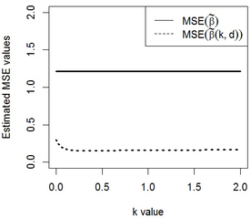
We consider a data set, which is known as the Egyptian pottery data to show the behavior of the new Restricted and Unrestricted Two-Parameter Estimators. This data set arises from an extensive archaeological survey of pottery production and distribution in the ancient Egyptian city of Al-Amarna. The data consist of measurements of chemical contents (mineral elements) made on many samples of pottery using two different techniques, NAA and ICP (see Smith et al. [30] for description of techniques). The set of pottery was collected from different locations around the city. We fit the data set by linear mixed model as ${\textstyle {\mathit {\boldsymbol {y}}}=}$${\mathit {\boldsymbol {X\beta }}}+{\mathit {\boldsymbol {Zu}}}+{\mathit {\boldsymbol {\epsilon }}},$ where ${\textstyle {\mathit {\boldsymbol {y}}}}$ is ${\textstyle 159\times 1}$ vector of response variables, ${\textstyle {\mathit {\boldsymbol {X}}}}$ and ${\textstyle {\mathit {\boldsymbol {Z}}}}$ which are regression matrix with dimensions ${\textstyle 159\times 6}$ and ${\textstyle 159\times 25}$ respectively. First, we are estimated the variance components by consider ${\textstyle {\sigma }_{1}^{2}=}$$0.5$ and ${\textstyle {\sigma }^{2}=0.5.}$ Then, by calculating the eigenvalues of ${\textstyle {\mathit {\boldsymbol {X}}}{\mathit {\boldsymbol {H}}}^{-1}{\mathit {\boldsymbol {X}}},}$ the condition number 8322860 is obtained, which indicate severe multicollinearity. We considered the stochastic linear restrictions as ${\textstyle {\mathit {\boldsymbol {r}}}=}$${\mathit {\boldsymbol {R\beta }}}+\Phi ,\Phi \sim N\left(0,{\sigma }^{2}{\mathit {\boldsymbol {I}}}_{3}\right)$ and selected 3 available data in the previous sections to the Egyptian pottery data. ${\textstyle {\tilde {k}}_{HM}}$ and ${\textstyle {\tilde {d}}_{opt}}$ are obtained using the iterative method introduced at the end of section 5,0.348 and 0.373 respectively. In Table 2, the estimated ${\textstyle MSE}$ values of the estimators are obtained by replacing in the corresponding theoretical MSE equations. We can see the estimated MSE values of ${\textstyle {\tilde {\mathit {\boldsymbol {\beta }}}}(k,d)}$ is less than ${\textstyle {\tilde {\mathit {\boldsymbol {\beta }}}}}$. Also, the estimated MSE values of ${\textstyle {\tilde {\mathit {\boldsymbol {\beta }}}}_{c}(k,d)}$ is less than ${\textstyle {\tilde {\mathit {\boldsymbol {\beta }}}}_{r}}$. In general, the estimated MSE values of ${\textstyle {\tilde {\mathit {\boldsymbol {\beta }}}}_{r}(k,d)}$ is less than all estimators. So, we conclude that the stochastic restricted two parameter estimator performs better than the other estimators. Note that in the results obtained for this data, all eigenvalues of ${\textstyle {\Delta }_{1}}$ and ${\textstyle {\Delta }_{2}}$ are positive and the condition of Theorem 4.1 and Theorem 4.2 are true. In Figure 1, a plot of the estimated MSE values of ${\textstyle {\tilde {\mathit {\boldsymbol {\beta }}}}}$ and ${\textstyle {\tilde {\mathit {\boldsymbol {\beta }}}}(k,d)}$ against ${\textstyle k}$ in the interval [0,2] with fixed ${\textstyle {\tilde {d}}_{opt~}=}$$0.373$ is drawn. Because ${\textstyle {\tilde {\beta }}}$ is not dependent on ${\textstyle k}$, its estimated ${\textstyle MSE}$ value is the same for all ${\textstyle k}$ values. It is obvious that estimated ${\textstyle MSE}$ values of ${\textstyle {\tilde {\mathit {\boldsymbol {\beta }}}}(k,d)}$ is always less than ${\textstyle {\tilde {\mathit {\boldsymbol {\beta }}}}}$. Altogether, it is obvious that the two parameter estimators can perform better than the ${\textstyle {\tilde {\mathit {\boldsymbol {\beta }}}}}$ in MSEM criterion under conditions.

Table 2. Estimated MSE values of the proposed estimators

	${\tilde {\mathit {\boldsymbol {\beta }}}}{\,}{\,}{\,}$	${\tilde {\mathit {\boldsymbol {\beta }}}}_{r}$	${\tilde {\mathit {\boldsymbol {\beta }}}}(k,d)$	${\tilde {\mathit {\boldsymbol {\beta }}}}_{r}(k,d)$
EMSE	1.216069	1.201379	0.1544953	0.1541745

Figure 1. The estimated mean square error values of the estimators versus ${\textstyle k}$ with ${\textstyle {\tilde {d}}_{of~}}$

8. Conclusion

In this article, we proposed the two parameter estimator and the stochastic restricted two parameter estimator to overcome the effects of the multicollinearity problem in linear mixed models. We also obtained estimates of variance parameters and then using the mean squared error matrix sense made comparisons between the proposed estimators and some other estimators. Finally, we proposed methods for estimating biasing parameters and provided a simulation study and a data example to illustrate performance of new estimators.

Disclosure statement

No potential conflict of interest was reported by the authors..

Funding

The research was supported by the Slamic Azad University.

References

[1] Zenzile T.G. Community health workers' understanding of their role in rendering maternal, child and women's health services. Diss. North-West University, 2018.

[2] Fiona S., Dierenfeld E.S., Langley-Evans S.C., Hamilton E., Lark R.M., Yon L., Watts M.J. Potential bio-indicators for assessment of mineral status in elephants. Sci. Rep-UK., 10(1):1-14, 2020.

[3] Rajat K., Guler I., Nerkar A. Entangled decisions: Knowledge interdependencies and terminations of patented inventions in the pharmaceutical industry. Strateg. Manage. J., 39(9):2439-2465, 2018.

[4] Adam, L., Corsi D.J., Venechuk G.E. Schools influence adolescent e-cigarette use, but when? Examining the interdependent association between school context and teen vaping over time. J. Youth. Adolescence, 48(10):1899-1911, 2019.

[5] Zhiyi C., Zhu S., Niu Q., Zuo T. Knowledge discovery and recommendation with linear mixed model. IEEE Access., 8:38304-38317, 2020.

[6] Henderson C.R. Estimation of genetic parameters. Ann. Math. Stat., 21:309–310, 1950.

[7] Henderson C.R., Searle S.R., VonKrosig C.N. Estimation of environmental and genetic trends from records subject to culling. Biometrics, 15:192–218, 1959.

[8] Farebrother R.W. Further results on the mean square error of ridge regression. J. Royal. Stat. Soc., Series B (Methodological), 38(3):248-250, 1976.

[9] Liu K. A new class of biased estimate in linear regression. Commun. Statist. Theor. Meth., 22(2):393–402, 1993.

[10] Liu X.Q., Hu P. General ridge predictors in a mixed linear model. J. Theor. Appl. Stat., 47:363–378, 2013.

[11] Yang H., Chang X. A new two-parameter estimator in linear regression. Commun. Statist. Theor. Meth., 39:923–934, 2010.

[12] Theil H., Goldberger A.S. On pure and mixed statistical estimation in economics. Int. Econ. Rev., 2:65–78, 1961.

[13] Theil H. On the use of incomplete prior information in regression analysis. J. Amer. Statist. Assoc., 58,401–414, 1963.

[14] Gilmour A.R., Cullis B.R., Welham S.J., Gogel B.J., Thompson R. An efficient computing strategy for predicting in mixed linear models. Comput. Statist. Data Anal., 44:571–586, 2004.

[15] Jiming J., Lahiri P. Mixed model prediction and small area estimation. Test., 15(1):1-96, 2006.

[16] Patel S.R., Patel N.P. Mixed effect exponential linear model. Commun. Statist. Theor. Meth., 21(9):2721-2740, 1992.

[17] Eliot M.N., Ferguson J., Reilly M.P., Foulkes A.S. Ridge regression for longitudinal biomarker data. Int. J. Biostat., 7:1–11, 2011.

[18] Özkale M.R., Can F. An evaluation of ridge estimator in linear mixed models: an example from kidney failure data. J. Appl. Statist., 44(12):2251–2269, 2017.

[19] Kuran O., Ózkale M.R. Gilmour’s approach to mixed and stochastic restricted ridge predictions in linear mixed models. Linear. Algebra. Appl., 508:22–47, 2016.

[20] Hartley H.O., Rao J.N. Maximum-likelihood estimation for the mixed analysis of variance model. Biometrika, 54:93–108, 1967.

[21] Lee Y., Nelder J.A. Generalized linear models for the analysis of quality-improvement experiments. Canad. J. Stat., 26(1):95–105, 1998.

[22] Hoerl A.E., Kennard R.W. Ridge regression: biased estimation for non-orthogonal problems. Technometrics, 12:55–67, 1970.

[23] Hoerl A.E., Kennard R.W. Ridge regression: iterative estimation of the biasing parameter. Commun. Statist. Theor. Meth., 5:77–88, 1976.

[24] Wencheko E. Estimation of the signal-to-noise in the linear regression model. Statist. Pap., 41:327–343, 2000.

[25] Kibria B.M. Performance of some new ridge regression estimators. Commun. Statist. Simul. Computat., 32:419–435, 2003.

[26] Mallows C.L. Some comments on Cp. Technometrics, 15:661–675, 1973.

[27] McDonald G.C., Galarneau D.I. A monte carlo evaluation of some ridge-type estimators. J. Amer. Statist. Assoc., 70:407–416, 1975.

[28] Golub G.H., Heath M., Wahba G. Generalized cross-validation as a method for choosing a good ridge parameter. Technometrics, 21::215–223, 1979.

[29] Craven P., Wahba G. Smoothing noisy data with spline functions. Numer. Math., 31:377–403, 1978.

[30] Smith D.M., Hart F.A., Symond R.D., Walsh J.N. Analysis of Roman pottery from Colchester by inductively coupled plasma spectrometry. Sci. Archaeolog. Glasgow, 196:41-55, 1987.