Joint optimization of condition-based maintenance and inventory ordering based on status monitoring for multi-unit system

Abstract

In the modern industry, in order to reduce the inventory pressure, a variety of parts began to use unified kind spare parts for maintenance. However, highly integrated equipment is more difficult to use traditional RCM models, and researchers begin to steering based on state monitoring methods. Deepen a prediction of equipment failure. This paper mainly discussed the data-driven analysis method based on the Wiener process to predict the fault law of the same type. The joint model innovatively adopts the ($s-1$, $s$) policy considering the industrial characteristic and multi-period resupply. In the end, we analyze ($s-1$, $s$) policy in joint optimization by comparison to draw the optimal policy combination.

Keywords: Multi-unit system, condition-based maintenance, spare parts, joint optimization, wiener process, resupply

1. Introduction

In industrial, military, and other fields, with the emergence of high-precision, high-information, and highly integrated equipment, the traditional fault prediction based on RCM using classical fault law experience shows some limitations in the more complex systematic analysis [1]. With the development of sensor technology, many researchers began to establish equipment life degradation model based on data-driven analysis, so as to predict the law of equipment failure [2].

The main methods in estimating life degradation based on data drive are: Gamma process, Gaussian inverse process, and Wiener process. After the exploration of many researchers, the data-driven model can be adapted to more and more modeling environments and can be used flexibly by adjusting formula parameters and expanding formulas [3]. So far, it has been widely used in the field of reliability [4-6]. Compared with the characteristics of the three models, the Gamma process and Gaussian inverse process are only suitable for modeling monotone degradation paths. In contrast, the Wiener process is more suitable for non-monotonic degradation processes caused by repair, self-healing, or use intensity [7]. It is also an important prerequisite for choosing a proper inventory policy [8].

In the research of inventory policy, the application amount of inventory policies is very high [9]. As two kinds of the most basic and classical inventory policies, they are still widely used in the modern supply chain. From the optimization goal, the ($T$, $S$) policy focuses on optimizing the inspection cycle $T$, while the ($s$, $S$)’s is the number of inventory resupply ($s$). Condition-based maintenance (CBM) is the more complicated preventive maintenance policy. The ($s$, $S$) policy which pays more attention to the change of inventory is closer along with the characteristics of CBM which based on the state of parts [10]. However, due to the high importance of the equipment using the data-driven method, the inventory cost and the loss caused by failure are also high, so in industrial practice, the factories which have this kind of equipment mostly adopt the ($s-1$, $s$) policy. After a part is replaced, the resupply application will be sent to replenish the inventory level.

Secondly, most of the delay time of inventory is fixed in all resupply periods. This fixed model is feasible in a certain time range. But for some industrial processes with multiple periods and a wide range of time in each period, the delay time also fluctuates with the influence of the transportation environment, local policy, or human factors [11]. In view of this characteristic, this article models the delay time separately and chooses the Poisson distribution which is generally accepted in the current research field to discuss [12] That is why simulating the multi-period resupply process.

The rest of this paper is organized as follows. Section 2 is the fault analysis method based on Wiener process and the research on the joint model between maintenance and inventory ordering. Then, section 3 mainly introduces performance degradation, life prediction by Wiener process, and CBM policy. In section 4, according to the conditions and constraints, combined with the ($s-1$, $s$) policy, the maintenance-inventory joint policy under the same type of multi-component condition monitoring is modeled. Besides that, the model of multi-period resupply time is also analyzed. Section 5 adopts Monte Carlo simulation and improved particle swarm optimization (PSO) algorithm to optimize the joint model and the optimal decision combination by balancing the model parameters. In section 6, a numerical example is given. While the sensitivity analysis of the resupply parameter, the corresponding comparison between the two kinds of inventory policies shows the difference. Conclusions and future work are given in section 7.

2. Literature review

2.1 Performance degradation process based on Wiener process

The Wiener process is one of the commonly used methods for modeling product performance degradation process in reliability assessment based on monitoring data [7]. The degradation process is a random process, driven by BM and Brownian motion. It is usually used to establish a model in the nonlinear degradation process.

In the current research, this kind of model has gradually developed to general and nonlinear problems related to time or state [13]. Baraldi, Mangili, Zio et al. sort out the diversity of model research, including time diversity, unit diversity, measurement diversity, and structural diversity [14]. Another point of the study is to consider the impact of the working environment on the performance degradation process. Bian, Gebraeel, Bian, Gebraeel et al. add covariates in the Wiener process as the environmental factors in the formula [15].

The model based on the Wiener process has also been applied to the field of spare parts. Elwany, Gebraeel et al. firstly combine the maintenance decision based on the Wiener process with the spare parts ordering to evaluate the optimal replacement and ordering time. They finally put forward the general framework of the joint policy as well [16]. After that, Zhang and Chen tried to introduce the Bayesian model into the joint decision model, and update the model parameters with real-time performance data [17]. On the other hand, Zhang and Chen extend the decision-making process to propose a random order lead time for inventory [18].

2.2 Inventory policy

Maintenance policy leads to inventory policy [19]. Talking about all inventory policies, according to the optimization goal, it can be divided into two main aspects. One is mainly represented by the inventory policies whose research goal is check cycle ($T$), such as ($T$, $S$) and ($T$, $Q$) [20]. However, in the long-term research, experts found it has limitation in applying due to the uncertainty of actual demand [21]. Therefore, the rigid and fixed inventory policies are difficult to meet the needs of multiple maintenance policies. Researchers began to discuss another kind of inventory policy represented mainly by ($s$, $S$) and ($s$, $Q$) policy [10,22,23]. The corresponding situation of parts leads to the change of inventory. In this view, the current number of inventory ($s$) is the focus of optimization.

However, there is a reality that with the development of technology, especially sensors, the reliability of parts has been gradually changed. The coin has two sides. A large number of spare parts are piled up in the warehouse, so it will result in a substantial increase in the proportion of inventory cost to the total cost. Lots of spare parts in some smaller warehouses cannot be transferred. What's more, there could be a large number of faulty spare parts and losses resulting from it. Considering the developed Internet and logistics industry, the researchers put forward the ($s-1$, $s$) policy. This policy aims to resupplied spare parts. After the part is replaced, the resupply information will be sent out. Sherbrooke firstly developed the policy into METRIC model under the limited cost and minimum out-of-stock [24]. After that, Grave proposed a simple algorithm for this research, which can be used in calculation [25].

2.3 Joint optimization

In the joint optimization of maintenance and inventory policy, considering the diversity and complexity, the previous literature focuses on traditional failure laws, such as Exponential distribution, Poisson distribution, and so on [26]. In recent years, data driven fault analysis was gradually developed. The joint optimization research based on that has been begun to discuss, especially the Wiener process.

Wang [27] applied the Wiener process to the joint optimization of CBM and inventory. Using the method of remaining life predicted by monitoring data, he analyzed the optimal policy for single part system [28,29]. With the deepening of the research on the single-part model, the research on multiple parts has been paid more and more attention. Minou and Nguyen [30] combined the Markov process and genetic algorithm with multi-period joint optimization for multiple parts, which is based on the ($s$, $S$) policy. Reviewing the previous research, there are few studies in the joint optimization of CBM based on the Wiener process and the ($s-1$, $s$) policy. Apart from that, most of the joint optimization studies focus on the parameters of maintenance policy, but there are few studies on the influence of inventory policy parameters, especially the time model of multi-period inventory delay.

3. Maintenance policy based on Wiener process

3.1 Notations

Table 1 shows a set the notations.

Table 1. Notations list

Symbol	Meaning	Unit
$k$	Index of customers ($k=1,2,3\cdots K$)
$\tau$	Index of check cycles ($\tau =1,2,3\cdots \Psi$)Ψ
$\tau _{i}$	Index of resupply periods ($\tau _{i}=1,2,3\cdots \Phi$)
$L$	Failure threshold
$n_{k}$	Index of equipment owned by customer $k$
$L_{n_{k}p}$	Threshold of preventive maintenance for the $n_{k}^{th}$part
$\mu$	Mean value	Use cycle
$\sigma$	Magnetic moment
$E_{n_{k}}^{\tau }$	Monitoring data of $n_{k}^{th}$ part in period $\tau$
$T_{c}$	Interval time between the two check cycles	Use cycle
$T_{n_{k}}^{\tau }$	Predicted residual life of $n_{k}^{th}$ part in period $\tau$ in theory	Use cycle
$t^{\tau }$	Time of check cycle	Use cycle
$C_{c}$	Unit check cost	yuan
$C_{pf}$	Unit cost of preventive maintenance	yuan
$C_{pr}$	Unit cost of collective maintenance	yuan
$C_{s}$	Unit delay loss	yuan
$C_{k}$	Unit inventory cost	yuan
$C_{b}$	Unit ordering cost	yuan
$S$	Maximum of inventory level
$s_{k}^{\tau }$	Current inventory level in customer $k$ in period $\tau$	yuan
$Q_{k}^{\tau _{i}}$	Number of spare parts replenishments of customer $k$ in resupply period $\tau _{i}$
$Q_{k}^{\tau _{i}}$	Spare parts consumption of customer $k$ in resupply period $\tau _{i}$
$t_{k}^{o{\tau }_{i}}$	Start time of resupply in customer $k$ in resupply period $\tau _{i}$	Use cycle
$T_{k}^{o{\tau }_{i}}$	Interval time of inventory delay in resupply period $\tau _{i}$	Use cycle
$t_{k}^{r\tau _{i}}$	Ending time of resupply in customer $k$ in resupply period $\tau _{i}$	Use cycle
$N_{c}$	Amount times of checking
$N_{pf}$	Amount times of preventive maintenance
$N_{pr}$	Amount times of collective maintenance
$N_{o}$	Amount of ordering
$N_{s}$($t^{\tau }$)	Amount of delay parts from $t^{\tau ^{-1}}$ to $t^{\tau }$
$N_{v}$ ($t^{\tau }$)	Amount of inventory at $t^{\tau }$

3.2 Life distribution

Suppose p-dimensional random vector, as (1) following:

$E(t)=[E_{1}(t),E_{2}(t),E_{3}(t)\cdots E_{p}(t)]{}'$

(1)

It is satisfying $p$-meta continuous stochastic processes {$E(t)$, $t\geq 0$} that concluded the following natures [31]:

(1) Assume initial quantity is $E(t)=(0,0,0\cdots 0)$. When $t=0$, $E(t)$ is continuous.

(2) $\Delta E=E(t+\Delta t)-E(t)$ shows the changing amount between $t+\Delta t$ and $t$. It obeys $p$-dimensional normal distribution

$\Delta E\sim N(\Delta t\mu ,\Delta t\sigma )$

(2)

where $\mu$ is the mean value and $\sigma$ is the standard deviation, as (3) and (4) following:

$\mu {}'=({\begin{array}{cccc}{\mu }_{1}{\mbox{ }}&{\mu }_{2}&{\mbox{ }}{\mbox{ }}{\mbox{ }}\cdots &{\mu }_{\mbox{p}}\end{array}}{\mbox{ }}{\mbox{ }}){}'{\mbox{ }}{\mbox{ }}{\mbox{ }}$

(3)

${\mbox{ }}\sigma ={\mbox{ }}{\mbox{ }}{\mbox{ }}{\mbox{ }}{\mbox{ }}{\mbox{ }}{\mbox{ }}{\mbox{ }}{\mbox{ }}{\mbox{ }}{\mbox{ }}{\mbox{ }}{\mbox{ }}{\mbox{ }}{\mbox{ }}{\mbox{ }}\left({\mbox{ }}{\mbox{ }}{\mbox{ }}{\begin{array}{cccc}{\sigma }_{1}^{2}&{\sigma }_{12}^{}&{\mbox{ }}{\mbox{ }}\cdots &{\sigma }_{1p}^{}\\{\sigma }_{12}^{}&{\sigma }_{2}^{2}&\cdots &{\sigma }_{2p}^{}\\\vdots &\vdots &\ddots &{\sigma }_{3p}^{}\\{\sigma }_{1p}^{}&{\sigma }_{2p}^{}&{\sigma }_{3p}^{}&{\sigma }_{p}^{2}\end{array}}\right){\mbox{ }}{\mbox{ }}$

(4)

Then regard

${\rho }_{xy}={\frac {{\sigma }_{xy}}{{\sigma }_{x}{\sigma }_{y}}}$

(5)

as the correlation coefficient of $E_{x}(t)$ and $E_{y}(t)$, ($x,y=1,2\cdots p$, $x\neq y$).

(3) In any two non-adjacent time intervals [$t_{1}$, $t_{2}$] and [$t_{3}$, $t_{4}$] $(t_{1}$< $t_{2}$< $t_{3}$< $t_{4})$, the respective increments $E(t_{4})-E(t_{3})$ and $E(t_{2})-E(t_{1})$ are independent of each other.

If satisfying, $E(t)$ is regarded as a Wiener process. The Normal distribution satisfied by the increment contains the parameters of the Wiener process.

If $B(t)$ is defined as a standard Brownian motion, that is, the univariate Wiener process can be expressed as shown in (6):

$E(t)=\mu t+\sigma B(t)$

(6)

where $\mu$ is the drift parameter, $\sigma$ is the diffusion parameter in this formula. Because of long-term use, the parts are bound to fail so that $\sigma$ is higher $0(\sigma >0)$. From (6), $E(t)$ is Brownian motion with linear drift [32].

According to the hypothesis and definition, each increment of the multivariate Wiener process obeys independent Normal distribution and belongs to non- monotonic Markov process. The mean value and variance of them are:

$E(E(t))=\mu t$

(7)

$Var(E(t))={\sigma }^{2}t$

(8)

Because $E(t)$ is a Wiener process, $E_{x}(t)$ which is its arbitrary row vector is also a Wiener process. It is also subject to (6). If the performance degradation process in a product conforms to it and the degradation value reaches the failure threshold ($L$), the product is determined to be a failure. The life time ($T$) can be defined as the time when the first performance of that degrades to $L$:

$T=\inf \lbrace t\vert E(t)=L,t\geq 0\rbrace$

(9)

The reference [33] shows that the life distribution is subject to the inverse Gaussian distribution so as to obtain the probability density function (PDF) and life distribution function (LDF). As (10) and (11) following:

$f(t)={\frac {L}{\sqrt {2\pi {\sigma }^{2}t^{3}}}}\exp \left[-{\frac {{\left(L-\mu t\right)}^{2}}{2{\sigma }^{2}t}}\right]$

(10)

$F(t)=\Phi \left({\frac {\mu t-L}{\sigma {\sqrt {t}}}}\right)+$$\exp \left({\frac {2\mu t}{{\sigma }^{2}}}\right)\Phi \left({\frac {-L-\mu t}{\sigma {\sqrt {t}}}}\right)$

(11)

As a result, the expectation and variance of $T$ are determined to be as (12) and (13):

$E(T)={\frac {L}{\mu }}$

(12)

$D(T)={\frac {L{\sigma }^{2}}{{\mu }^{3}}}$

(13)

where $E(t)$ is the expectation value and $D(t)$ is the variance value.

Secondly, the parameters are determined. In references [29,30,31], $\mu$ and $\sigma$ are estimated by the method of maximum likelihood estimation. Suppose to get the data through monitoring the degradation process. Then, these can be calculated by preprocessing. According to the definition of LDF, what is the difference value between the current data and the former is subject to Normal distribution.

Likelihood function can be established by the former steps, as (14) follow:

$L(\mu ,{\sigma }^{2})=\prod _{x=1}^{n_{k}}\prod _{y=1}^{m_{k}}{\frac {1}{\sqrt {2{\sigma }^{2}\pi \Delta t_{x}^{y}}}}\exp \left[-{\frac {{\left(\Delta E_{x}^{y}-\mu \Delta t_{x}^{y}\right)}^{2}}{2{\sigma }^{2}\pi \Delta t_{x}^{y}}}\right]$

(14)

The maximum likelihood estimation value of $\mu$ and σ are as follow (15) and (16):

${\overset {\mbox{ˆ}}{\mu }}={\frac {\displaystyle \sum _{x=1}^{n_{k}}E_{x}^{y}}{\displaystyle \sum _{x=1}^{n_{k}}t_{x}^{y}}}$

(15)

${\hat {\sigma }}=\left\{{\frac {1}{\displaystyle \sum _{x=1}^{n_{k}}{m_{k}}}}\left[\sum _{x=1}^{n_{k}}{\displaystyle \sum _{y=1}^{m_{k}}{\displaystyle {\frac {\left(\Delta E_{x}^{y}\right)^{2}}{\Delta t_{x}^{y}}}}}-\displaystyle {\frac {\left(\displaystyle \sum _{x=1}^{n_{k}}{E_{x}^{m_{k}}}\right)^{2}}{\displaystyle \sum _{x=1}^{n_{k}}{t_{x}^{m_{k}}}}}\right]\right\}^{2}$

(16)

Following the former steps, the performance degradation function of parts based on the Wiener process can be established.

3.3 Condition-based maintenance

From the former, the system gets $E_{n_{k}}^{\tau }$ at $t^{\tau }$ by the continuous check. In modern industry, the economic cost caused by long-term reliance on corrective maintenance is getting higher and higher. It is generally accepted that the preventive maintenance policy can improve the availability of equipment. For the maintenance needs time, especially the delay loss in production is relatively high, the maintenance department generally replaces the part directly. There are two main ways in CBM, which are corrective and preventive maintenance.

By the collective maintenance, it would be happened in $t^{\tau }$, when the part is failed in the interval time from $t^{\tau ^{-1}}$ to $t^{\tau }$. For the preventive maintenance, the $n_{k}^{th}$ part will be under that process when $E_{nk}^{\tau }$ is up to $L_{n_{k}p}$. Because the failure may lead to other concurrent failures, the associated parts should be thoroughly examined when the replacement is carried out. Resulting from it, $C_{pr}$ will be higher than $C_{pf}$ ($C_{pr}>C_{pf}$).

Secondly, in order to avoid delay loss as much as possible, the part will be executed the preventive maintenance when its degradation value is not up to $L$ so that it can avoid collective maintenance in the turning process to next check cycle. That’s as (17) following:

$F(t^{\tau })=\Phi \left({\frac {\mu t^{\tau }-L_{n_{k}p}-E_{n_{k}}^{\tau }}{\sigma {\sqrt {t^{\tau }}}}}\right)+$$\exp \left({\frac {2\mu t^{\tau }}{{\sigma }^{2}}}\right)\Phi \left({\frac {-L_{n_{k}p}-E_{n_{k}}^{\tau }-\mu t^{\tau }}{\sigma {\sqrt {t^{\tau }}}}}\right)>\alpha$

(17)

When $E_{n_{k}}^{\tau }$ is up to the threshold of preventive maintenance or collective maintenance, the part will be replaced with a new one if there are spare parts in inventory.

However, it is likely to occur that the spare parts are in delay in reality. In this case, there is still a delay before replacing. The parts that cannot undergo preventive maintenance will continue to be used in order to decrease delay cost. But if the resupply is gotten, the maintenance will continue. The parts which are going to be collective maintenance will be replaced firstly. What’s more, the replacing time is so short than the lifetime that it is ignored when modeling.

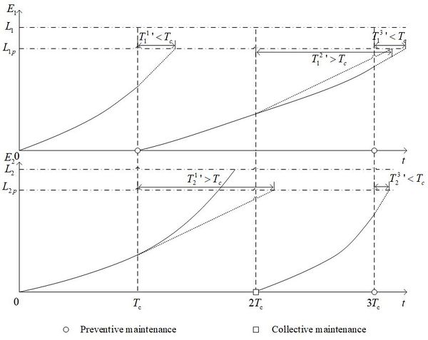
Take the condition-based maintenance process for two types of parts as an example. The initial degradation value $E_{n_{k}}^{1}$ is 0. Figure 1 shows the main process of condition-based maintenance.

Figure 1. Condition-based maintenance process of two parts

In Figure 1, $E_{1}^{1}$ which is the degradation value of the first part at $t^{1}$ is lower than $L_{1_{p}}(E_{1}^{1}<L_{1_{p}})$ which is its threshold value of preventive maintenance. But the predicted residual life $T_{1}^{1'}$ is less than $T_{c}$ ($T_{1}^{1'}<T_{c}$). So, the part is under preventive maintenance at this time. Turn to $t^{2}$ which is the second check cycle. The degradation value $E_{1}^{2}$ which is the degradation value at the current cycle is also lower ($E_{1}^{2}<L_{1_{p}})$. Different from roe former time, the predicted residual life $T_{1}^{2'}$ is higher than $T_{c}$ $(T_{1}^{2'}>T_{c})$. So, it needn’t be paired. However, turn to $t^{3}$, the situation is similar to that in $t^{1}$. The part is going to be under preventive maintenance as well.

Next to talking about the second part. At $t^{1}$, $E_{2}^{1}$ which is the degeneration value of second part is lower than $L_{2_{p}}(E_{2}^{1}<L_{2_{p}})$ which is its threshold of preventive maintenance. According to former formulas, the predicted residual life $T_{2}^{1'}$ is less than $T_{c}$ $(T_{2}^{1'}>T_{c})$. So, it needn’t to brplacedweve. Hor, in the interval time between $t^{1}$ and $t^{2}$, there is a failure in the part. It caused the breakdown loss. Apart from that, the part won’t be replaced because it isn’t reached the check cycle. It didn’t begin the collective maintenance until it is at $t^{3}$. Turning to the next check cycle, $E_{2}^{3}$ which is the current degeneration value is lower than $L_{2_{p}}(E_{2}^{3}<L_{2_{p}})$. But $T_{2}^{3'}$ which is the current predicted residual life is less than $T_{c}$ $(T_{2}^{3'}>T_{c})$. The part is replaced at this time.

4. Joint maintenance-inventory policy

4.1 Propose a joint policy

($s-1$, $s$) policy is one of the new aspects in modern inventory policy. For some valuable parts, it is often adopted and requires monitoring of inventory. Assuming that in the beginning, the $k^{th}$ inventory is up to the $S$. The parts couldn’t degenerate in inventory. Once the replacement happens, the resupply applicant will be sent out.

It takes time for spare parts from application to arrival. During it, the parts on work are still performing. So, $Q_{k}^{\tau _{i}}$ is not only determined by $\Delta s_{k}^{\tau }$ which is the difference value in period $\tau$ between $S$ and $s_{k}^{\tau }$, but also $Q_{k}^{\tau _{i}}$’ which is the consumptions in $\tau _{i}$.

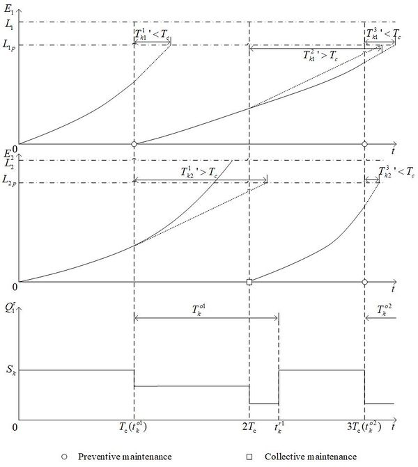
Still take the condition-based maintenance process of the two parts mentioned in Figure 1 as an example. It supposes the $k^{th}$ customer owns these two types of parts. The parts play an important role in each machine and consume the same kind of spare parts. So, the threshold of them is the same ($L_{1}=L_{2}$ and $L_{1_{p}}=L_{2_{p}}$). We can make a decision in inventory ordering. That is as Figure 2 following.

Figure 2. Analysis process in maintenance and inventory for the two kinds of parts

At $t^{1}$, the first part has completed the preventive maintenance, but the degradation of the second part does not meet the replacement conditions. So, the inventory decreases 1. At the same time, the resupply application is sent. Turning to $t^{2}$, the first part has not replaced, and the second part is under collective maintenance. So, the inventory continues to decrease 1. However, the system can’t send the application because it has done in the former cycle. Time changes to $t^{3}$. The first part is under preventive maintenance. As for the second part, the condition of preventive maintenance has been reached. So, the inventory decreases 2. At the same time, the customer has gotten the first resupply so that the second resupply application can be sent.

4.2. Resupply of spare parts

As Figure 2 following, the first resupply application is sent to the system at $t^{1}$. When the application is sent, $t^{1}$ is also $t_{k}^{o^{1}}$ which is the start time of the first resupply. Spending $T_{k}^{o^{1}}$ which is the delay time of the first inventory resupply, it goes to $t_{k}^{r^{1}}$ which is the ending time. At this time, the first resupply has finished. $t_{k}^{r^{1}}$ is equal to $t_{k}^{o^{1}}$ and $T_{k}^{o^{1}}$ $(t_{k}^{r^{1}}=t_{k}^{o^{1}}+T_{k}^{o^{1}})$. Turning to $t^{3}$, the second resupply application is sent. The process is the same as the former. $t^{3}$ is also $t_{k}^{o^{2}}$ which is the start time of the second resupply. $t_{k}^{r^{1}}$ which is the ending time is determined by not only $t_{k}^{o^{2}}$, but also $T_{k}^{o^{2}}$ which the delay time of the second inventory resupply $(t_{k}^{r^{2}}=t_{k}^{o^{2}}+T_{k}^{o^{2}})$. As a result, they can be obtained that the inventory delay time, start time and, ending time in every resupply period.

However, the spare parts which are adopted ($s-1$, $s$) policy generally need long-term and multi-period resupply. Therefore, it is unreasonable for the previous fixed delay time model to continue to be used in this kind of spare parts. In this article, it is assumed that the delay time satisfies the Poisson distribution.

5. Modeling in joint policy

For the same kind of parts that adopt data monitoring to estimate the residual life. Too frequent inspection cannot provide a more accurate data basis for the life prediction. What’s more, it may affect the fitting speed of fault function based on the Wiener process because of the large amount. At the same time, this behavior will continue to increase the cost of testing, resulting in excessive cost.

On the contrary, it may increase the probability of part failure in the next inspection that $T_{c}$ is too large so that it could lose the significance of preventive maintenance policy. Secondly, if $L_{n_{k}p}$ is too high, it will increase the times and the ordering cost. Apart from the two aspects, increasing maximum inventory could affect the inventory cost as well. What’s more, the decreasing inventory may cause the delay loss so that the availability of equipment will be affected.

In conclusion, the joint policy of maintenance and inventory ordering focuses on adjusting the decision variables which are $T_{c}$, $S$ and $L_{n_{k}p}$ to control the costs of preventive maintenance, collective maintenance, check, ordering even delay loss. Under the condition of certain equipment reliability, it may reduce the total cost as much as possible to obtain the optional joint combination of corresponding decision variables.

When calculating the joint model, there are mainly two methods. One is establishing an accurate set of formulas after a complete mathematical derivation. But it is difficult to use explicit expressions to clearly express the relationship between objective functions and decision variables. Then, the joint optimization for the same kind of multi-type parts in this article is a logical process triggered randomly at a discrete time by the change of decision variables. Another is the Marko simulation. It can solve this kind of problem well. By adjusting the decision parameters and analyzing a large number of simulations, the value distribution of objective function in this interval of time is obtained to get the optional joint policy.

The objective function adopted the expense cost rate ($EC$) to calculate the joint model. It is argued the target of $EC$ is minimum in this model, as (18) following:

$\min EC_{\infty }=\min f_{EC}(T_{c},S,L_{n_{k}p})$

(18)

Because the monitoring object is the same kind of parts, their threshold values of preventive maintenance are all roughly the same, (18) can be adjusted to (19):

$\min EC_{\infty }=\min f_{EC}(T_{c},S,L_{p})$

(19)

$s.t.$

$\quad t^{\tau }=\tau \times T_{c},\,\,\tau =1,2,3\cdots \psi$

$T_{c}>0$

$S\in N^{+}$

$L_{p}>0$

According to the method in calculating $EC_{\infty }$ from reference [34], it can be changed to (20):

$EC_{\infty }={\underset {t_{m}\rightarrow \infty }{\lim }}\displaystyle {\frac {C_{c}\cdot N_{c}+C_{pf}\cdot N_{pf}+C_{pr}\cdot N_{pr}+C_{o}\cdot N_{o}+C_{s}\cdot \displaystyle \sum _{\tau =1}^{\psi }N_{s}(t^{\tau })+C_{v}\cdot \displaystyle \sum _{\tau =1}^{\psi }N_{v}(t^{\tau })}{t_{m}\cdot N}}$

(20)

However, it is a relatively large project to use Monte Carlo simulation to logically analyze the maintenance-ordering process. It spends so much time and achieved a little part for the whole process. In order to speed up the optimization rate and reduce the cost-effectiveness ratio of research, an intelligent optimization algorithm is used. It not only speeds up the calculation, but also provides ways to the real-time decision-making inventory for the same kind of spare parts in the future. The particle swarm optimization (PSO) algorithm is chosen among all intelligent optimization algorithms in this article

The PSO algorithm is one of the most widely used algorithms in multi-period model optimization [35]. It is paid attention to by researchers because of its easy implementation, high precision, fast convergence, and so on. It has demonstrated its superior algorithm characteristics in practical applications. What’s more, the PSO algorithm is also a parallel algorithm. It can improve the efficiency of optimization by making full use of the parallel computing advantages of processors.

5.1 PSO algorithm

In the field of algorithm research, there are many new algorithms emerging in endlessly. Many researchers combine the advantages of different algorithms to improve [36].

Whether it is the traditional algorithm or the new intelligent algorithm, it is mainly divided into two kinds: heuristics and meta-heuristics. It has been recognized by more and more researchers that the optimization policy can be obtained quickly by using the PSO algorithm. However, the convergence effect of the traditional PSO algorithm is not satisfactory because of the diverse and complex conditions in the joint model. Therefore, some researchers combine the algorithm with dynamic optimization [37], and some researchers introduce adaptive weight into the algorithm [38].

The improved PSO algorithm from reference [39] is adopted in this article to solve multi-period continuous optimization problems. It adjusts the convergence weight of particles in global and local optimization by combining the nonlinear dynamic inertia weight used to detect the global optimal point and the penalty factor of dynamic correction. It can adapt to the characteristics of multi-period iteration in this model to improve the convergence rate of calculation.

5.2 Maintenance and ordering

1) Initialization

Firstly, initialize $E_{n_{1}}^{0}$, $E_{n_{2}}^{0}$, $E_{n_{3}}^{0}\cdots E_{n_{k}}^{0}$. Those are the initial state of parts. And then, initialize the parameters by inputting, such as $T_{c}$, $S$, $L_{p}$ , $\mu$, $\sigma$, $n_{K}$, $\Phi$, $K$, $L$, $\sigma$, $T_{kn_{k}}^{0}$, $C_{c}$, $C_{pf}$, $C_{pr}$, $C_{o}$, $C_{s}$, $C_{v}$.

Before turning to the general degradation process, the system will pay attention to whether there is resupply getting or not. As (21) following:

$OR_{k}^{\tau }=\left\{{\begin{array}{c}{\begin{array}{cc}0&\left(t_{k}^{rt_{i}}/T_{c}\leq \tau \right)\cup \left(OR_{k}^{\tau -1}=1\right)\\OR_{k}^{\tau -1}&{\mbox{others}}\end{array}}{\mbox{ }}\end{array}}\right.$

(21)

where $OR_{k}^{\tau }$ is the resupply applicant remark. When there is resupply getting, it is updated to ‘$OR_{k}^{\tau }=0$’. If not, it will be the same as the former. In the beginning, there is no resupply. ‘$OR_{k}^{\tau }=0$’ will be updated to 1.

2) Maintenance for Delay Parts

The system will replace the parts whose collective maintenance process is a delay. As (22) following:

$SPN_{n_{k}}^{\tau }=\left\{{\begin{array}{c}{\begin{array}{cc}0&\left(SPN_{n_{k}}^{\tau -1}{\mbox{=}}1\right)\cup \left(s_{k}^{\tau }>0\right)\\SPN_{n_{k}}^{\tau -1}&{\mbox{others}}\end{array}}\end{array}}\right.$

(22)

where $SPN_{n_{k}}^{\tau }$ is the delay mark in the current cycle, $SPN_{n_{k}}^{\tau -1}$ is the mark in the last cycle. When the parts are replaced, $SPN_{n_{k}}^{\tau }$ will be changed to 0.

Because of the maintenance, it needs a spare part to replace. $SPPF_{n_{k}}^{\tau }$ and $s_{k}^{\tau }$ are updated as (23) and (24) following:

$SPPF_{n_{k}}^{\tau }=1$

(23)

$s_{k}^{\tau }=s_{k}^{\tau }-1$

(24)

3) Degradation Process

From the former life prediction analysis, the process of $n_{k}^{th}$ degradation changing at a continuous point of time could be as (25) following:

$E_{n_{k}}^{\tau }=E_{n_{k}}^{\tau -1}{\mbox{+}}\Delta E_{n_{k}}^{\tau }$

(25)

where $\Delta E_{n_{k}}^{\tau }$ which obeys Normal distribution is a random increment at the interval time from $\tau -1$ to $\tau$, as (26) following:

$\Delta E_{n_{k}}^{\tau }(T_{c})=\mu \cdot T_{c}+\sigma \cdot B(T_{c})$

(26)

According to section 3, the state of $n_{k}$ in $\tau$ is as (27) and (28) following:

$SiF_{n_{k}}^{\tau }=\left\{{\begin{array}{cc}2&E_{n_{k}}^{\tau }\geq L\\0&E_{n_{k}}^{\tau }<L\end{array}}\right.$

(27)

$SiF_{n_{k}}^{\tau }=\left\{{\begin{array}{cc}1&E_{n_{k}}^{\tau }\geq L_{p}\\0&E_{n_{k}}^{\tau }<L_{p}\end{array}}\right.$

(28)

1) When the value of degradation reaches $L$, the part is a failure. If there is inventory, it will be going to collective maintenance. It sets a remark which there is a part that need collective maintenance. As (27) following.

2) When the degradation value is lower than $L$, the part is normal. However, it may need preventive maintenance.

3) When the degradation is lower than $L_{p}$, the part is normal. Except that, the system will predict the life degradation of part. If $T_{n_{k}}^{\tau }$’ is shorter than $T_{c}$ ($T_{n_{k}}^{\tau }<T_{c}$) and there is inventory in $k^{th}$ customer. It will be going to preventive maintenance. As Equation (29) following:

${\mbox{ }}SiF_{n_{k}}^{\tau }=\left\{{\begin{array}{cc}1&\left({\mbox{ }}SiF_{n_{k}}^{\tau }=0\right)\cup \left(T_{n_{k}}^{\tau }{}'<T_{c}\right)\\0&{\mbox{others}}\end{array}}\right.$

(29)

where $SiF_{n_{k}}^{\tau }$ is the preparation mark of preventive maintenance.

4) When the degradation value is up to $L_{p}$, the part will be going to preventive maintenance. As (28) following.

In conclusion, Equations (27), (28) and (29) can be sum up into to (30):

$SiF_{n_{k}}^{\tau }=\left\{{\begin{array}{cc}2&E_{n_{k}}^{\tau }\geq L\\1&\left(\left({\mbox{ }}E_{n_{k}}^{\tau }<L_{p}{\mbox{ }}\right)\cup \left(T_{n_{k}}^{\tau }{}'<T_{c}\right)\right)\cap \left(E_{n_{k}}^{\tau }\geq L_{p}\right)\\0&{\mbox{others}}\end{array}}\right.$

(30)

4) Inventory Changing

Before replacing, the system will check the inventory. The amount of preventive and collective maintenance will be marked. For it, the replacement mark is set to mark the process. As (31) and (32) following:

$SPPF_{n_{k}}^{\tau }=\left\{{\begin{array}{cc}1&\left(SiF_{n_{k}}^{\tau }=1\right)\cup \left(s_{k}^{\tau }>0\right)\\0&{\mbox{others}}\end{array}}\right.$

(31)

$SPRF_{n_{k}}^{\tau }=\left\{{\begin{array}{cc}1&\left(SiF_{n_{k}}^{\tau }=2\right)\cup \left(s_{k}^{\tau }>0\right)\\0&{\mbox{others}}\end{array}}\right.$

(32)

where $SPRF_{n_{k}}^{\tau }$ is the preventive maintenance mark, $SPRF_{n_{k}}^{\tau }$ is the collective maintenance mark. When there is inventory, it will finish the corresponding maintenance. When there is little inventory, the replacement process will be delayed. So, $SPN_{n_{k}}^{\tau }$ is updated, as (33) following:

$SPN_{n_{k}}^{\tau }=\left\{{\begin{array}{c}{\begin{array}{cc}1&\left(SiF_{n_{k}}^{\tau }=2\right)\cup \left(s_{k}{\mbox{=}}0\right)\\SPN_{n_{k}}^{\tau }&{\mbox{others}}\end{array}}\end{array}}\right.$

(33)

When there is little inventory, the process of parts that are going to collective maintenance will be delayed. It is marked ‘$SPN_{n_{k}}^{\tau }=1$’. But the parts which are going to preventive maintenance will continue to be used because of no inventory. What's more, when inventory is insufficient, priority is given to the parts which are going to collective maintenance.

After maintenance, the number of inventories will be updated. As (34) following:

$s_{k}^{\tau }=\left\{{\begin{array}{c}{\begin{array}{cc}s_{k}^{\tau }-1&SPF_{n_{k}}^{\tau }=1{\mbox{ }}\\s_{k}^{\tau }{\mbox{ }}&{\mbox{others}}\end{array}}{\mbox{ }}\end{array}}\right.$

(34)

Then the state of parts would be changed because of the maintenance. As (35) following:

$E_{n_{k}}^{\tau }{}'=\left\{{\begin{array}{cc}E_{n_{k}}^{\tau }&{\mbox{others}}\\0&{\mbox{ }}\left(SPPF_{n_{k}}^{\tau }{\mbox{=}}1\right)\cap \left(SPRF_{n_{k}}^{\tau }=1\right)\end{array}}\right.$

(35)

where $E_{n_{k}}^{\tau }$' is the final value of degradation in this part in the current check cycle. When the part is replaced, the degradation will recalculate. If not, it will go on declining. There is one more word that the degradation process wouldn’t be affected by monitoring. Because of that, the start time of life for this part is determined whether to replace or not. The residual life is as (36) following:

$T_{kn_{k}}^{\tau }{}'=\left\{{\begin{array}{cc}T_{kn_{k}}^{0}&\left(SPPF_{n_{k}}^{\tau }=1\right)\cap \left(SPRF_{n_{k}}^{\tau }=1\right)\\T_{kn_{k}}^{\tau }&other\end{array}}\right.$

(36)

where $T_{kn_{k}}^{\tau }{}'$ is the final value of residual life for this part, $T_{kn_{k}}^{0}$ is the initial life. When the part is replaced, it will be recalculated. If not, the final residual life is equal to the theoretical value in current check period.

5) Ordering

Once the inventory decreases, the resupply applicant would be sent at once. So, $OR_{k}^{\tau }$ will be updated, as (37) following:

$~OR_{k}^{\tau }{\mbox{=}}\left\{{\begin{array}{cc}1&\left(s_{k}^{\tau }<S\right){\mbox{ }}\cap \left(OR_{k}^{\tau }=0\right)\\0&{\mbox{others}}\end{array}}\right.$

(37)

The resupply period is started to be calculated. When the resupply applicant is sent, $\tau _{i}$ will be updated as (38) following:

$~{\tau }_{i}={\tau }_{i}+1$

(38)

At the same time, the parameters of resupply would be marked, such as $t_{k}^{o{\tau }_{i}}$, $T_{k}^{o{\tau }_{i}}$, $t_{k}^{r{\tau }_{i}}$. As (39) following:

$t_{k}^{o{\tau }_{i}}modT_{c}=0$

(39)

$T_{k}^{o{\tau }_{i}}$ obeys Poisson distribution, as (40) following:

$T_{k}^{o{\tau }_{i}}={\frac {a^{{\tau }_{i}}}{{\tau }_{i}!}}\cdot e^{-a}$

(40)

where $\tau _{i}$ belongs to the positive integer ($\tau _{i}=1,2,3\cdots \Phi$ ).

From the former sections, $t_{k}^{r{\tau }_{i}}$ is determined by delay time of inventory and the start time of resupply, as (41) following:

$t_{k}^{r{\tau }_{i}}=T_{k}^{o{\tau }_{i}}+t_{k}^{o{\tau }_{i}}$

(41)

What's more, $Q_{k}^{{\tau }_{i}}$ is made up of $\Delta s_{k}$ and $Q_{k}^{{\tau }_{i}}{}'$, as (42) following:

$Q_{k}^{{\tau }_{i}}=\Delta s_{k}+Q_{k}^{{\tau }_{i}}{}'=S_{k}-s_{k}^{\tau }+Q_{k}^{{\tau }_{i}}{}'$

(42)

$\Delta s_{k}$ and $Q_{k}^{{\tau }_{i}}{}'$ are determined by the state of parts. With the resupply getting, the inventory is updated. As (43) following:

$s_{k}^{\tau }=\left\{{\begin{array}{cc}s_{k}^{\tau -1}+Q_{k}^{{\tau }_{i}}&OR_{k}^{\tau }=0\\s_{k}^{\tau -1}&{\mbox{others}}\end{array}}\right.$

(43)

5.3. Calculating EC_∞

When the decisions of maintenance and inventory policies are made in one check cycle, the values of $N_{pf}$, $N_{pr}$, $N_{c}$, $N_{s}$ and $N_{v}$ are updated. As the formulas following:

$~N_{pf}=N_{pf}+\sum _{n_{k}=1}^{n_{K}}SPPF_{n_{k}}^{\tau }$

(44)

$~N_{pr}=N_{pf}+\sum _{n_{k}=1}^{n_{K}}{\mbox{ }}SPRF_{n_{k}}^{\tau }$

(45)

$~N_{c}=N_{c}+n_{K}$

(46)

$~N_{s}=\sum _{n_{k}=1}^{n_{K}}SPN_{n_{k}}^{\tau }$

(47)

$~N_{v}=\sum _{n_{k}=1}^{n_{K}}s_{k}^{\tau -1}$

(48)

It is necessary that the system should update the value of the check cycle. As (49) following:

$~\tau =\tau +1$

(49)

When the system turns to the next check cycle, $\tau$ will be updated. The simulation process will back to the ‘initialization’ section and go along with the former process period by period. What’s more, it is the once simulation.

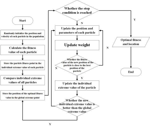
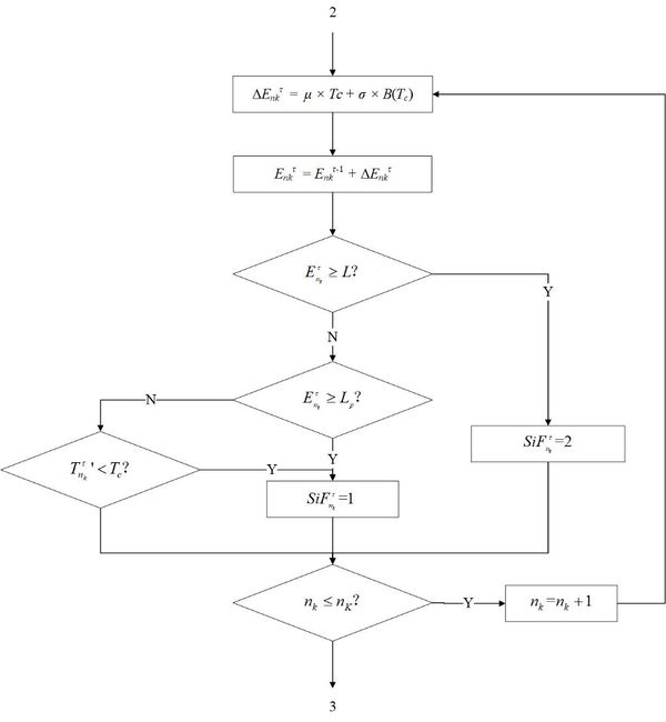
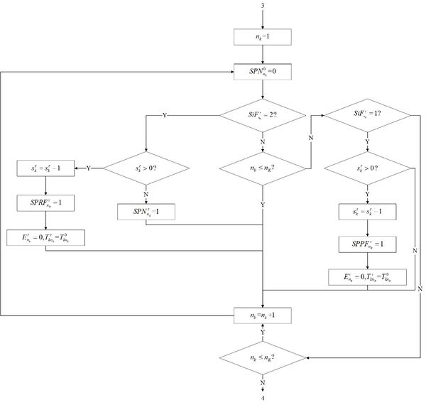
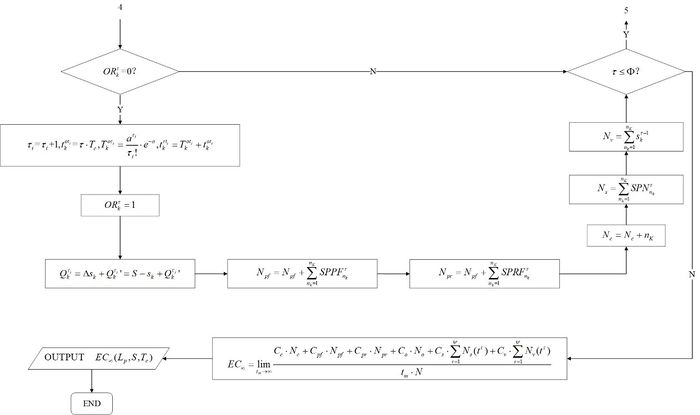
Before the simulation, the researching duration of the model l should be made clear. It would be divided into several check cycles to get discrete syncopation points. The process of maintenance and inventory ordering is simulated by the Monte Carlo method. With the iteration of the check cycle, the changes of parts and inventory in each cycle are deduced. Through the cumulative calculation of costs for all cycles, the expected cost rate of a simulation is obtained finally. This is once result of a simulation. The system will process multi-period simulation by adopting the adaptive improved PSO algorithm. The algorithm is as Figure 3 following, which expands the optimization process of decision variables $T_{c}$, $S$, $L_{p}$ in the function of $EC_{\infty }$.

Figure 3. Iterative optimization process of the improve PSO algorithm

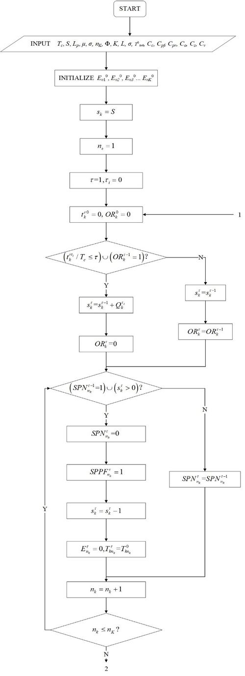
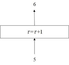
To sum up, the whole joint policy is following Figures 4(a), (b), (c), (d) and (e) to get the optional decision combination ($T_{c}^{*}$, $S^{*}$, $L_{p}^{*}$) under the minimum average expense rate. Where $T_{c}^{*}$ is the optional check cycle, $S^{*}$ is the optional inventory, $L_{p}^{*}$ is the optional threshold of preventive maintenance. Figure 4(a) is the part of simulation and maintenance for delay parts. Figure 4(b) is the general degradation part. Figure 4(c) is the part of inventory. Figure 4(d) is the periodic intermediate process. Figure 4(e) is the ordering part of resupply.

(a) The once process of simulation (part I)

(b) The once process of simulation (part II)

(c) The once process of simulation (part III)

(d) (d) The once process of simulation (part IV)

(e) The once process of simulation (part V)

Figure 4.

6. Numerical investigation

6.1 Case description

In automotive engines, because of the core position of the engine in the composition of the vehicle, especially racing cars, the fault monitoring of engine (internal combustion engine) and the subsequent maintenance procedure has always been the important contents that researchers pay close attention to. From the view of the maintenance department, the internal combustion engine has two main characteristics. First is its mechanical structure being complex, in order to ensure the tightness of the cylinder and the completeness of combustion. For example, the cylinder of a gasoline internal combustion engine is generally made by pouring with an integrated mold. Apart from it, there are lots of parts loading in the engine, such as bearings, pistons, flywheels.

The subtle hidden trouble caused by any one part may lead to the failure in the engine. Another one is that most of the main body of the automobile engine is generally embedded in the automobile interior so that the general self-test program cannot check whether there is any obvious fault on the outside of the engine. What's more, it’s too hard to check the interior of the engine. Therefore, the German Volkswagen Group, General Motors of the United States, Toyota of Japan, and other companies gradually began to use electronic monitoring and control technology to carry out real-time monitoring of engines and other key components. On the one hand, the central control system notifies the maintenance team belonging to the fleet. On the other hand, it may send the fault analysis report to the customer center belonging to the depot through the remote platform as well. When the vehicle enters the maintenance workshop, the maintenance personnel can download the monitoring data from the central control system for data analysis, so as to provide options for later maintenance and provide suggestions for the improvement of the car to the R&D department of the car company.

According the data from a fleet which is in the interval of time from 2012 to 2017, the team is mainly responsible for the maintenance and modification of 10 vehicles in the fleet, including training, racing, and spare vehicles. All vehicles are monitored for the part of the engineer. According to reference [42], the data was preprocessed. Then the data is processed based on performance degradation modeling. The process does not belong to the main content of this article, so it will not be elaborated here. The result is as Table 2.

Table 2. Statistical results of data analysis

No.	g1	g2	$|\mu _{1}|$	$|\mu _{2}|$
1	0.4465	2.929	1.2532	0.722
2	-0.3172	2.7418	1.0619	1.1577
3	0.7363	3.0332	2.0687	1.7633
4	0.2786	2.9975	0.7838	1.4075
5	-2.445	2.6326	0.6725	2.0883
6	0.0526	2.9214	0.1487	0.6422
7	-0.082	2.7745	0.2304	0.8263
8	-0.2252	2.7765	0.605	0.6049
9	0.1047	2.6556	0.2942	2.0192
10	-0.154	2.6817	0.4327	1.7516

Where column 2-3 are the third-order center distance and fourth-order center distance in order to check the value of $k^{th}$ skewness and kurtosis, column 4-5 is the parameter value of statistical test.

Assume that $\alpha$ which is the significance level for determining whether the degradation process of that can be express by the Wiener process is equal to 0.05. If the value of $|\mu _{1}|$ and $|\mu _{2}|$ are both less than $Z_{\alpha }/4$, the data can be used by this method. It is known that $Z_{\alpha }/4$ is equal to 2.25. So, the values of column 3 and 4 aren’t higher than 2.25. After checking, the degradation process can be expressed by Wiener process.

Maintenance and inventory costs have fluctuated over the past 6 years. Resulting from it, we considered the impact of economic purchasing power fluctuations on modeling in this article to process the cost data of 6 years. The calculated costs of every aspect are as Table 3 following.

Table 3. List of costs after processing

	$C_{c}$	$C_{pf}$	$C_{pr}$	$C_{o}$	$C_{s}$	$C_{v}$
Fitness (Unit: yuan)	500	5000	20000	8000	30000	8000

According to the data, $t$ which is the whole optimization time is equal to 20000 use cycle. $C_{c}$ which is the unit check cost is equal to 500 yuan. When the degradation value is less than $L$, it is assumed that it is a failure. After it was finished the collective maintenance, the system would cost 20000 yuan which is the unit cost of collective maintenance ($C_{pr}$). It would turn back to the initial state until the replacement. However, there will be delay loss if no inventory. It may lead to the cost of personnel, equipment, and reputation because of the inability to carry out daily training, unnormal competitions and other planned schedule work. It is roughly 30000 yuan through calculating. In the meantime, the team will do some preventive maintenance while the value of degradation is less than $L_{p}$. It would cost 5000 yuan which is the unit cost of preventive maintenance.

The team adopted the ($s-1,\,s$) policy to manager. The inventory cost in every check cycle includes the lease of the warehouse, the salary of managerment, and the arrangement cost of the inventory environment. It is roughly 8000 yuan which is the unit inventory cost. It would not send the resupply applicant until there is no inventory. The ordering cost of unit spare part ($C_{o}$) is 8000 yuan.

6.2 Modeling in degradation

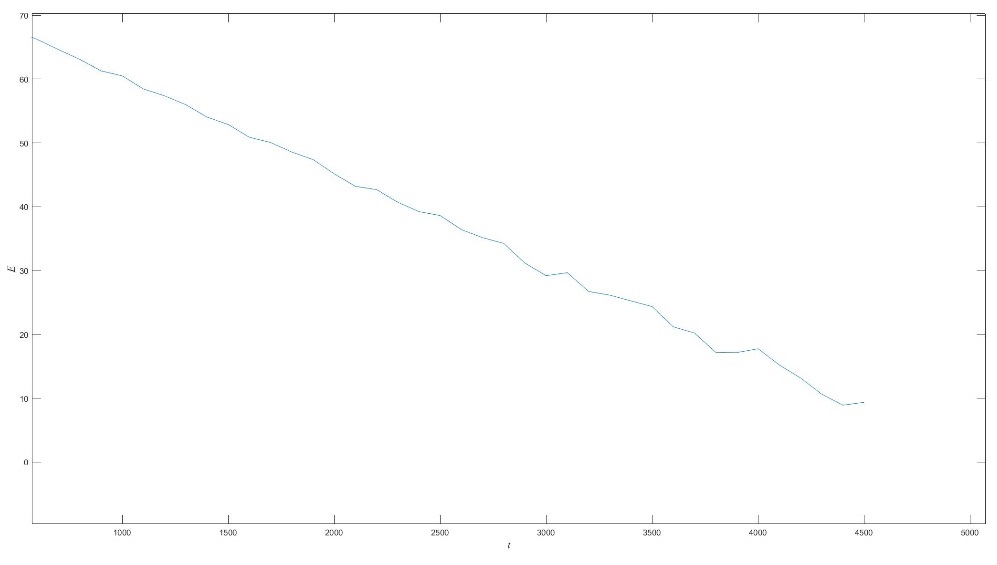
According to section 2, the maximum parameter estimation method is used to calculate the above data. what set the initial value of state is equal to 75 ($E_{n_{k}}^{1}=75$). They are calculated that ${\overset {\frown }{\mu }}$ which is equal to -0.01475 and ${\overset {\frown }{\sigma }}$ which is equal to 0.39985. The degradation process of internal combustion engine can use (50) to follow:

$~E(t)=75-0.01475t+0.39985B(t)$

(50)

Set the value of $L$ to 0. The whole process is simulated by Monte Carlo method.

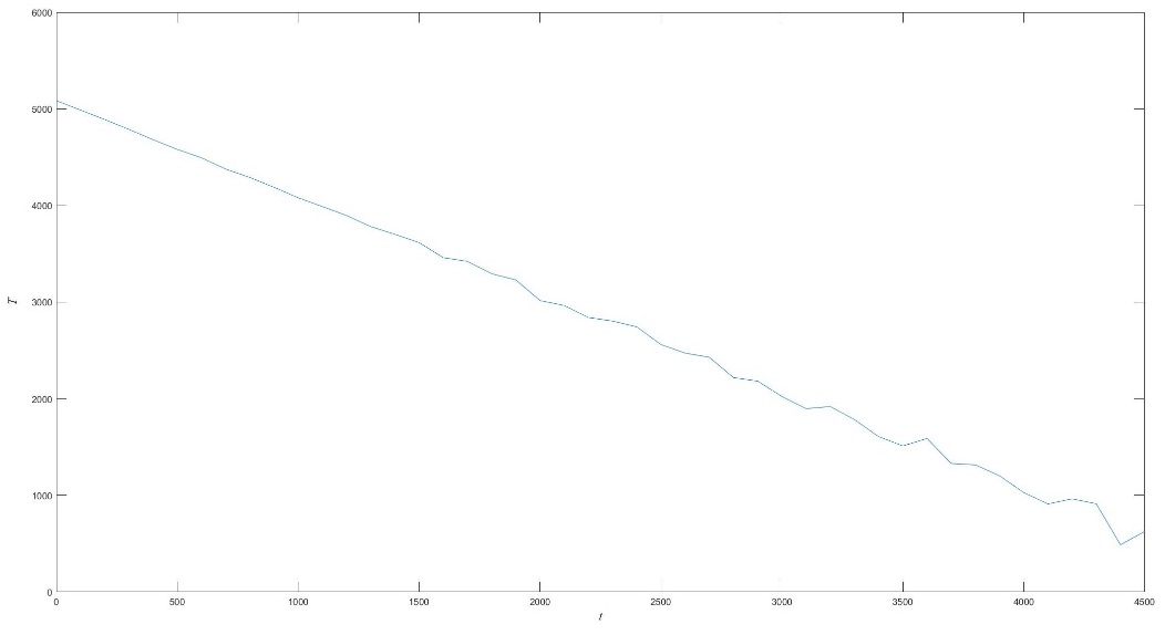
It is obvious that the state degraded with the time going in Figure 5. What's more, as time goes by, the offset increases gradually. Except that, it is possible that the predicted value of the next period is higher than the former. It’s the result in the deviation between the linear function and the linear function is getting larger and larger that the scope of Brownian motion is getting wider and wider with the time goes.

According to (12) and (13), the system would predict the residual life, as Figure 6 following.

Figure 5. Performance degradation curve obtained by Monte Carlo simulation

Figure 6. Life prediction of part in performance degradation process

6.3 Result analysis

From the equation of $EC_{\infty }$, the decision parameters which need optimization conclude: $T_{c}$, $S$, $L_{p}$. The improved PSO algorithm discussed in section 5 is used to optimize the joint policy.

In order to ensure the efficiency and accuracy of optimization, set the model parameters: $N$ which is the number of species is equal to 100, $c_{1}$ is equal to 1.6962 and $c_{2}$ is equal to 1.8962 which are the learning factors, $w_{\min }$ is 0.6 and $w_{\max }$ is 0.8 which are inertia weight minimum and maximum, $M$ which is the number of iterations is equal to 60. As for the resupply, the time of the first inventory delay is 300 use cycles. $a$ which is the parameter of resupply model is equal to 110.3640 through calculating. Those will be adopted to the optimization process. After that, the system got the optimal decision combination which is [$T_{c}^{*}$, $S^{*}$, $L_{p}^{*}$]. Where it is [1220,5,8]. The mean value of the expense cost rate is 133.835 yuan. The convergence process is as Fig. 7 following.

From Figure 7, the objective function curve tends to be smooth in the last stage of the convergence process, and the fluctuation range of the end decreases gradually. At the same time, the penalty function also tends to be flat, and the value of the function tends to 0. As Figure 8 following, it’s a conclusion that the convergence effect is good so that the result is the optimal solution after optimization. The optional decision combination shows a fact that the fleet should adjust the check cycle to do one check after 1220 use cycles. On the one hand, the maintenance department should execute the policy of collective maintenance by monitoring. On the other hand, it should obey the policy of preventive maintenance when the value of degradation is less than 8. What’ 'sore, it’s a balance between maintenance efficiency and economic performance that the maximum inventory is set to 5. Once the replacement comes across, the resupply applicant will be sent to ensure the next maintenance.

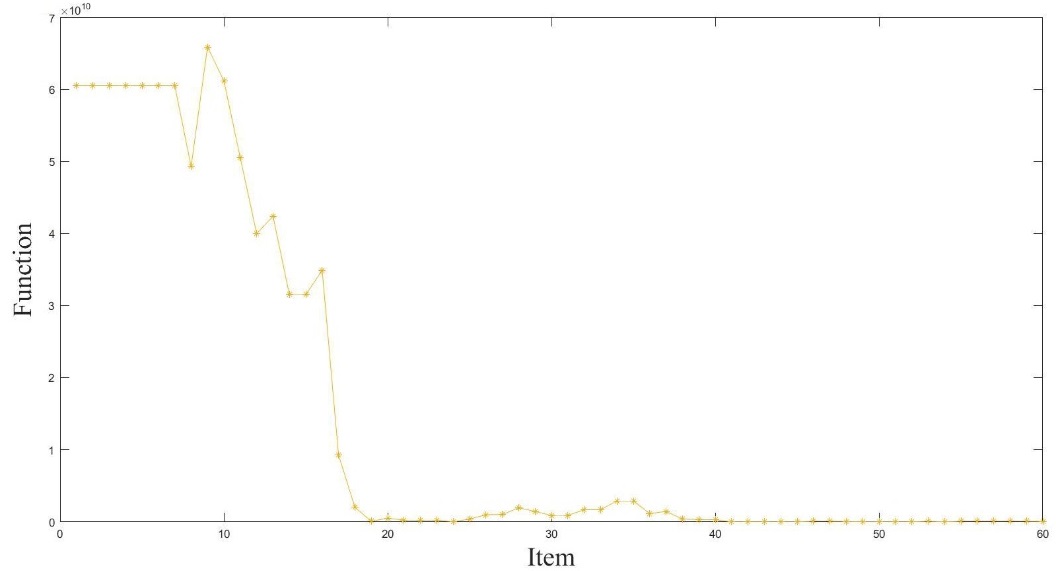
Figure 7. Objective function change process by improved PSO algorithm

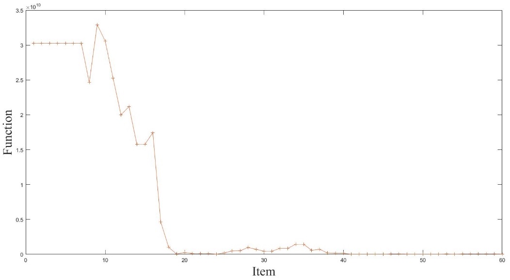
Figure 8. Penalty function change process by improved PSO algorithm

In references [40,41], the researchers analyzed the influence of parameters on optimization results, such as cost and fault threshold. There has been a comprehensive sensitivity analysis as far. However, the model is built for the multi-type parts of the same kind. The discussion of the new joint policy focuses on the resupply time model to study. And then, the parameters of resupply model are the next targets for discussion. As Table 4 following, the result of sensitivity analysis in $a$ is gotten.

From Table 4, with the value of $a$ is higher, the delay time of resupply will be longer. It causes the value of $T_{c}^{*}$, $S^{*}$, $L_{p}^{*}$ to get higher so that the expense cost rate is also higher. That's easy to be understood. Considering the availability of machines and delay cost, it will do some measures to solve it. One is up to inventory to avoid delay. Another one is up to the threshold of preventive maintenance to decrease the possibility of collective maintenance. However, those methods both result in the higher cost. The first causes the higher cost of inventory. The second cost of preventive maintenance is higher. On the other hand, when the value of a decreases, the delay time of inventory and the decision parameters don’t decrease as predicted. On the contrary, the threshold of preventive failure increases. In refence [42], the researcher has discussed the numerical analysis in the updating process of multi-period ($s$, $S$) policy. It can be inferred that the probability of delay in spare parts is greatly reduced when the time of resupply is reducing. Because of it, the center of optimization changes to the maintenance policy from the inventory policy. The optional joint policy points out it that does well in reducing the total cost through raising the threshold of preventive maintenance appropriately. It reduced the cost of collective maintenance, while the cost of preventive maintenance is getting higher.

Table 4. Sensitivity analysis in parameters of resupply model

No.	$a$	$T_{c}$	$S$	$L_{p}$	$E(EC_{\infty })$
1	183.9400	1260	8	11	148.690
2	147.1520	1240	6	10	144.185
3*	110.3640	1220	5	8	133.835
4	73.5759	1217	5	10	134.305

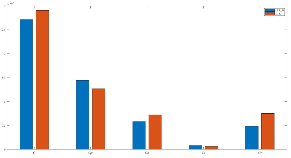
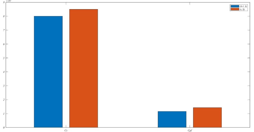
What's more, the model is adopted ($s-1$, $s$) policy. The optimization effect has been gotten by compared with the ($s$, $S$) policy. The result is as Table 5 following. Under the same condition, the value of $S^{*}$ is smaller, while the values of $T_{c}^{*}$ and $L_{p}^{*}$ are higher in the ($s-1$, $s$) policy with the comparison of the ($s$, $S$) policy. Through analysis, the resupply applicant will be sent when the inventory begins to reduce. It is unnecessary that maintaining a relatively high inventory. It reduces the inventory cost, as Figure 9(a) and (b) following. Where the blue square stands for the cost of ($s-1$, $s$) policy, the red one is on behalf of the cost of ($s$, $S$) policy. However, the joint policy adopted ($s$, $S$) policy increases the check cycle and preventive maintenance threshold to avoid the cost of corrective maintenance, while the cost of collective maintenance is reduced.

Table 5. Comparison of the results of inventory strategy between ($s$, $S$) and ($s-1$, $s$) under the same conditions

Inventory policy	$T_{c}$	$L_{p}$	$S$	$s$	$E(EC_{\infty })$
($s-1$, $s$) policy	1220	8	5	/	135.484
($s-1$, $s$) policy	1160	6	7	2	145.254

(a) The comparison of every aspect of costs between the ($s-1$, $s$) policy and ($s$, $S$) policy (the part of $C$, $C_{pr}$, $C_{o}$, $C_{s}$, $C_{v}$)

(b) The comparison of every aspect of costs between the ($s-1$, $s$) policy and ($s$, $S$) policy (the part of $C_{c}$, $C_{pr}$)

Figure 9.

The optional decision combination adopted ($s$, $S$) policy needs the wider space for inventory either because of the larger number of maximum inventories. However, it is an important aspect of considering for some smaller factory or maintenance team, for example, the fleet discussed in this article. In conclusion, the joint policy adopted ($s-1$, $s$) policy will ensure the minimum cost under the certain maintenance efficiency.

7. Conclusion

The center of this article focuses on the joint policy of maintenance and inventory ordering for the multi-style of the same kind. Performance degradation model is obtained by using widespread life prediction methods based on the Winer-based process.

There is a fact that the condition of the model is very complex. The maintenance budget is relatively low for some customers so that the inventory space is the same. The ($s-1$, $s$) policy adopted in this model has some characteristics which can solve the problems, such as high-security efficiency, good economic benefits, and so on. Then, the resupply processes are multi-period and fluctuate changing. For this characteristic, the joint model has rebuilt the resupply process. We balanced to optimize the decision parameters which conclude check cycle, maximum inventory, and the threshold of preventive maintenance to get the optional decision combination. On the other hand, in order to reduce the cost-effectiveness ratio, the optimizing process is adopted the Monte Carlo method and the improved PSO algorithm.

Based on the joint model and optional decision combination, the effect of resupply model parameter on the optimization result is gotten. At the same time, the superiority of the optional policy is shown by the comparison with the result adopted by the ($s$, $S$) policy.

Those are the whole research results in this article. While providing optimal solutions for industries, they can also provide a feasible reference for the multi-style part of the same kind in complex maintenance environments.

References

[1] Friedlob G.T., Plewa F.J. Understanding return on investment. Wiley, New York, May 1996.

[2] Liu Z., Zhang L. A review of failure modes, condition monitoring and fault diagnosis methods for large-scale wind turbine bearings. Measurement, 149:107002, 2020.

[3] Le Son K., Fouladirad M., Barros A., Levrat E., Iung B. Remaining useful life estimation based on stochastic deterioration models: A comparative study. Reliab. Eng. Syst. Saf., 112:165–175, 2013.

[4] Chinnam R.B. On-line reliability estimation for individual components using statistical degradation signal models. Qual. Reliab. Eng. Int., 18:53–73, 2002.

[5] Whitmore G.A., Schenkelberg F. Modelling accelerated degradation data using Wiener diffusion with a time scale transformation. Lifetime Data Anal, 3:27–45, 1997.

[6] Robinson M.E. Bayesian methods for a growth-curve degradation model with repeated measures. Lifetime Data Anal., 6:357–374, 2000.

[7] Chiming G., Wang W., Guo B., Si X. A maintenance optimization model for mission-oriented systems based on Wiener degradation. Reliab. Eng. Syst. Saf., 111:183–194, 2013.

[8] Wang W. A stochastic model for joint spare parts inventory and planned maintenance optimization. Eur. J. Oper. Res., 216:127–139, 2012.

[9] Feeney G.J., Sherbrooke C.C. The (s − 1, s) inventory policy under compound Poisson demand. Manag. Sci., 12:391–411, 1966.

[10] Bashyam S., Fu M.C. Optimization of (s, S) inventory systems with random lead times and a service level constraint. Manag. Sci., 44:S243–S256, 1998.

[11] Shibuya T., Dohi T., Osaki S. Optimal continuous review policies for spare part provisioning with random lead times. Int. J. Prod. Econ., 55:257–271, 1998.

[12] Srinivasan S.K. Analysis of s, S inventory systems with general lead time and demand distribution and adjustable reorder size. Optimization, 19:557–576, 1988.

[13] Zhang Z., Si X., Hu C., Lei Y. Degradation data analysis and remaining useful life estimation: A review on Wiener-process-based methods. Eur. J. Oper. Res., 271:775–796, 2018.

[14] Wang H., Song W., Zio E., Kudreyko A., Zhang Y. Remaining useful life prediction for Lithium-ion batteries using fractional Brownian motion and Fruit-fly Optimization Algorithm. Measurement, 161:107904, 2020.

[15] Bian L., Gebraeel N. Stochastic modeling and real-time prognostics for multi-component systems with degradation rate interactions. IIE Trans., 46:470–482, 2014.

[16] Elwany A.H., Gebraeel N.Z. Sensor-driven prognostic models for equipment replacement and spare parts inventory. IIE Trans., 40:629–639, 2008.

[17] Zhang J.-L., Chen J. Bayesian solution to pricing and inventory control under unknown demand distribution. Oper. Res. Lett., 34:517–524, 2006.

[18] Zhang X., Zeng J. Joint optimization of condition-based opportunistic maintenance and spare parts provisioning policy in multiunit systems. Eur. J. Oper. Res., 262:479–498, 2017.

[19] Lee J., Ghaffari M., Elmeligy S. Self-maintenance and engineering immune systems: Towards smarter machines and manufacturing systems. Annu. Rev. Control., 35:111–122, 2011.

[20] Covert R.P., Philip G.C. An EOQ model for items with weibull distribution deterioration. AIIE Transactions, 5:323–326, 1973.

[21] Petrovic D., Roy R., Petrovic R. Supply chain modelling using fuzzy sets. Int. J. Prod. Econ.. 59:443–453, 1999.

[22] Hu Q., Boylan J.E., Chen H., Labib A. OR in spare parts management: A review. Eur. J. Oper. Res., 266:395–414, 2018.

[23] Rao U.S. Properties of the periodic review (R, T) inventory control policy for stationary, stochastic demand. Manuf. Serv. Oper. Manag., 5:37–53, 2003.

[24] Sherbrooke C.C. Metric: A multi-echelon technique for recoverable item control. Oper. Res., 16(1):122–141, 1968.

[25] Graves S.C. A multi-echelon inventory model for a repairable item with one-for-one replenishment. Manag. Sci., 31:1247–1256, 1985.

[26] Vaughan T.S. Failure replacement and preventive maintenance spare parts ordering policy. Eur. J. Oper. Res., 161:183–190, 2005.

[27] Wang Z., Wang W., Hu C., Liu X.. An integrated decision model for critical component spare parts ordering and condition based replacement with prognostic information. Chem. Eng. Trans., 33:1063–1068, 2013.

[28] Wang Z.-Q., Wang W. , Hu C.-H., Si X.-S., Zhang W. A prognostic-information-based order-replacement policy for a non-repairable critical system in service. IEEE Trans. Reliab., 64(2):721–735, 2015.

[29] Wang Z., Hu C., Wang W., Kong X., Zhang W. A prognostics-based spare part ordering and system replacement policy for a deteriorating system subjected to a random lead time. Int. J. Prod. Res., 53:4511–4527, 2015.

[30] Nguyen K.-A., Do P., Grall A. Condition-based maintenance for multi-component systems using importance measure and predictive information. Int. J. Syst. Sci. Oper. Logist., 1:228–245, 2014.

[31] Chhikara R.S., Folks L. The inverse Gaussian distribution: theory, methodology, and applications. M. Dekker, New York, November 1989.

[32] Gihman I.I., Skorokhod A.V. The theory of stochastic processes I. Springer Berlin Heidelberg, Berlin, Heidelberg, 2004.

[33] Jorgensen B., Seshadri V. The inverse Gaussian distribution: A case study in exponential families. J. Am. Stat. Assoc., 91(433):432+, 1996.

[34] Acharya D., Nagabhushanam G., Alam S.S. Jointly optimal block-replacement and spare provisioning policy. IEEE Trans. Reliab., 35:447–451, 1986.

[35] Leong W.-F., Yen G.G. PSO-based multiobjective optimization with dynamic population size and adaptive local archives. IEEE Trans. Syst. Man Cybern. Part B Cybern., 38(5):1270–1293, 2008.

[36] Nearchou A.C. The effect of various operators on the genetic search for large scheduling problems. Int. J. Prod. Econ., 88:191–203, 2004.

[37] Isah O.R., Usman A.D., Tekanyi A.M.S. A hybrid model of PSO algorithm and artificial neural network for automatic follicle classification. Int. J. Bioautomation, 21:43-58, 2017.

[38] Shao H., Zheng G. Boundedness and convergence of online gradient method with penalty and momentum. Neurocomputing, 74:765–770, 2011.

[39] Wang Y., Shi Q. Improved dynamic PSO-based algorithm for critical spare parts supply optimization under (T, S) inventory policy. IEEE Access, 7:153694–153709, 2019.

[40] Zuo M.J., Jiang R., Yam R.C.M. Approaches for reliability modeling of continuous-state devices. IEEE Trans. Reliab., 48:9–18, 1999.

[41] Xiao L. Joint optimization of condition-based maintenance and spare parts supply for the same type of multi-component system. Nanjing University of Aeronautics and Astronautics, Nanjing, 2016.

[42] Zhao F., Liu X. Joint optimization of periodic inspection and spare parts strategy considering imperfect maintenance. Theory and Practice of System Engineering, 37:3201–3214, 2017.