Abstract
This work explores the use of stabilized finite element formulations for the incompressible Navier-Stokes equations to simulate turbulent flow problems. Turbulence is a challenging problem due to its complex and dynamic nature and its simulation if further complicated by the fact that it involves fluid motions at vastly different length and time scales, requiring fine meshes and long simulation times. A solution to this issue is turbulence modeling, in which only the large scale part of the solution is retained and the effect of smaller turbulent motions is represented by a model, which is generally dissipative in nature.
In the context of finite element simulations for fluids, a second problem is the apparition of numerical instabilities. These can be avoided by the use of stabilized formulations, in which the problem is modified to ensure that it has a stable solution. Since stabilization methods typically introduce numerical dissipation, the relation between numerical and physical dissipation plays a crucial role in the accuracy of turbulent flow simulations. We investigate this issue by studying the behavior of stabilized finite element formulations based on the Variational Multiscale framework and on Finite Calculus, analyzing the results they provide for well-known turbulent problems, with the final goal of obtaining a method that both ensures numerical stability and introduces physically correct turbulent dissipation.
Given that, even with the use of turbulence models, turbulent flow problems require significant computational resources, we also focused on programming and parallel implementation aspects of finite element codes, and in particular in ensuring that our solver can perform efficiently on distributed memory architectures and high-performance computing clusters.
Finally, we have developed an adaptive mesh refinement technique to improve the quality of unstructured tetrahedral meshes, again with the goal of enabling the simulation of large turbulent flow problems. This technique combines an error estimator based on Variational Multiscale principles with a simple refinement procedure designed to work in a distributed memory context and we have applied it to the simulation of both turbulent and non-Newtonian flow problems.
1 Introduction
1.1 Background and motivation
1.1.1 Turbulence modeling
Turbulent flows are a subject of paramount interest in engineering, physics and earth sciences, since they govern many phenomena involving moving fluids like volumes of air or water. Turbulent phenomena appear in flows of all sizes, from large scale processes such as the atmospheric flow of air or oceanic currents to local problems such as wind loads over lightweight structures or the efficiency of a wind turbine. However, the complex nature of turbulent flows means that they can rarely be solved analytically and, as a result, we have to rely on experimental studies or numerical simulations for their analysis.
Experimental studies, which typically involve either campaigns of field measurements or wind tunnel tests, tend to be expensive and complex endeavors (see for example [1]) and, although they are an essential tool in providing a deeper understanding of the problem, tend to provide localized measurements such as point recordings or line averages, which are limited to the regions where sensors are placed, or indirect measurements, such as trajectories of tracers. From this point of view, numerical modeling represents a less costly alternative to experiments with the added advantage of providing a global image of the velocity and pressure fields for the entire volume of interest. Unfortunately, numerical study of turbulent problems is not without difficulty. The fundamental problem in turbulent flow simulations is the wide range of time and spatial scales involved [2], which have to be taken into account in the analysis.
Taking as an example the flow around an obstacle, the largest fluid motions, or eddies, in the flow can be assumed to have a characteristic size comparable to the size of the obstacle itself. Under a turbulent flow regime, coherent flow structures tend to break and the energy associated to these motions is transferred to successively smaller eddies until, for very localized fluctuations, viscous effects dominate and the energy is dissipated. This process can be formalized in terms of the energy associated to motions of a characteristic wavelength in what is known as the Kolmogorov energy cascade [3,4,2] and the size at which viscous dissipation dominates is defined as the Kolmogorov length .
Turbulent flows can be characterized by the Reynolds number , a dimensionless parameter indicative of the balance between inertial and viscous forces in the problem,
|
|
(1.1) |
where is the fluid's density and its dynamic viscosity and is a characteristic velocity of the flow. The Kolmogorov length scale can be related to the largest motions of the flow by means of the Reynolds number [2] as
|
|
(1.2) |
To properly represent the full range of turbulent motions in a numerical simulation, the size of the problem domain would be a multiple of the size of the obstacle on each dimension, while the grid size would have to be small enough to capture motions on the Kolmogorov scale. For a problem, this implies that the total number of elements would be on the order of . Keeping in mind that the Reynolds number in engineering applications is typically on the order of , the number of elements involved in a typical simulation would put it beyond the reach of most computers and scientific computation clusters. As a result, this approach, which is known as Direct Numerical Simulation (DNS) is only applicable to problems with a moderate Reynolds number and is not commonly used in engineering.
The only viable option in most cases is to introduce a turbulence model to reduce the computational requirements of the simulation. This typically involves neglecting the smallest motions and modifying the problem to include terms that model the effect of the neglected motions on the problem. The addition of such model increases the minimum element size required to simulate the problem, extending the range of problems that can be simulated with given computational resources. Turbulence models can be grouped into two broad families, Reynolds Averaged Navier-Stokes (RANS) and Large Eddy Simulation (LES).
RANS models are based on rewriting the problem in terms of time-averaged variables (or time- and space-averaged, if there are spatial directions of homogeneity) and introducing a model for the effect of turbulent motions on the averaged solution. This model has a dissipative effect, removing energy from the average motions, and most commonly takes the form of an added viscosity, called turbulent or eddy viscosity. The temporal and spatial distribution of the eddy viscosity is given by the specific model and is usually determined by the solution of one or more additional equations that describe the production and transport of turbulent quantities. Typical examples of RANS models are the Spalart-Allmaras model [5], which involves one additional equation, or the – [6,7] and – models [8], which introduce two additional variables.
LES models are based on introducing a spatial filter to smooth out high wave number fluctuations in the solution and writing the problem equations in terms of filtered quantities. This allows the separation of larger flow features, influenced by the geometry of the fluid domain and the boundary conditions, from the smaller motions, which are assumed to have an universal behavior and thus can be replaced by local dissipation model, which is problem-independent. The most well known member of this family of models is the Smagorinsky method [9], but many variants and alternatives exist [2].
Note that, while the use of turbulence models makes the simulation of turbulent flows possible in terms of mesh resolution and computational resources, many flows of practical interest still require fine meshes and long simulation times in order to obtain statistically steady solutions and reliable statistical measurements. As a result, the simulation of complex flows at high Reynolds number still requires significant computational resources, frequently beyond what a single computer can provide, and has to be solved using High Performance Computing (HPC) clusters.
1.1.2 Stabilized finite element formulations for turbulent flows
A second problem frequently encountered in the finite element simulation of incompressible flows is the apparition of numerical instabilities, which are a consequence of the incompressibility constraint and the effect of the convective term in the equations for convection-dominated flows (see for example [10] for an introduction to this topic). In the context of finite elements, one possible solution for this issue is the use of stabilization techniques, where the original Galerkin weak form of the problem is modified to obtain a stable formulation. The modified equations are characterized by the addition of new terms that are typically dissipative in nature, in a way that ensures consistency, that is, that the modified problem tends to the original equations as the simulation mesh is refined.
For turbulent flows in particular, the interaction between turbulence models and stabilization terms is an active area of research. While they have clearly different origins and motivations (turbulence models are typically motivated using physical arguments, while stabilization methods are purely numerical in nature), both types of methods have a dissipative effect on the solution, which has raised some questions regarding their interaction or the possibility of using a unified formulation to provide both stability and turbulence modeling. This subject has been studied for example for Streamline-Upwind Petrov-Galerkin (SUPG) stabilization [11,12], Finite Calculus (FIC) based formulations [13,14] and stabilization techniques within the Variational Multiscale (VMS) framework.
In the case of VMS formulations, the stabilized problem is motivated by a separation of scales, differentiating a large scale part of the solution, that can be represented by the finite element mesh, from a small scale part, which remains unresolved, by means of a projection of the solution onto the finite element mesh [15,16]. This concept has intriguing parallels with the spatial filtering introduced in LES methods and can be understood as a mesh-induced filtering. This has motivated multiple investigations studying the use VMS formulations in turbulence modeling [17,18,19,20,21,22,23,24,25,26,27], analyzing their relationship both from the theoretical point of view and through its application to the simulation of turbulent flows of interest.
1.2 Objectives and methodology
The main topic of this monograph is the study of the applicability of stabilized finite element techniques to the solution of turbulent flow problems of practical interest in engineering, with a special focus in analyzing the behavior of different formulations as a LES-like turbulence model. The research is organized around two main lines: The first of them is centered on stabilized finite element formulations and their relationship with turbulence modeling, while the second focuses on computational techniques to facilitate the calculation of complex flows in large simulation domains.
Regarding the relationship between stabilized formulations and turbulence modeling, we choose to focus on two types of methods. The first of them is the VMS framework, where we intend to analyze the behavior of two well-known formulations, algebraic subgrid scales and orthogonal subgrid scales, as well as dynamic subscales, while the second is a new formulation derived from the application of the FIC balance to the incompressible Navier-Stokes equations. We have implemented a fluid solver based on the different techniques and used it to analyze their performance.
The first topic that will be discussed in terms of the computational aspects of the present work is the use of parallel programming techniques for the simulation of finite element problems in a distributed memory context. In this sense, all developments have been made with a parallel implementation in mind, choosing algorithms and implementations that are suited to a parallel implementation in preference to alternatives that are not, and the parallel capabilities of the implemented code have been evaluated.
A related topic in relation to the calculation of large problems is the use of adaptive mesh refinement techniques to simplify the mesh generation procedure and reduce the overall number of elements required to perform the simulation. We have developed a technique based on a simple refinement technique that can work in a distributed memory environment, which has been implemented to work in combination with the fluid solver. During the course of the present work we also found the opportunity to apply these refinement techniques to non-Newtonian flow problems. The results of our investigation in this area will also be presented.
The methods presented in this document have been implemented within the open source Kratos Multiphysics finite element framework [28,29], which is based on C++ and Python and has parallel calculation capabilities, some of which have been developed or expanded as part of the present work. This implementation has been used to simulate all the examples considered and generate the presented results.
1.3 Outline of this document
The present document is organized along the main goals outlined above. In Chapter 2 we introduce VMS methods, with a special emphasis on dynamic subscale approximations, and review the arguments that have been used in the literature to relate them to LES formulations. Our tests have driven us to propose a variant of the method characterized by a new model for the pressure subscale. We use both the standard approach and our modified formulation to simulate a turbulent channel flow benchmark problem, which allows us to compare our results to DNS data.
In Chapter 3 we present a new stabilized formulation for incompressible flows based on the FIC balance principles. This formulation is also used to simulate the channel flow problem, as well as other benchmark examples.
Chapter 4 is concerned with different aspects of the parallel implementation of the finite element flow solver that has been used to perform the simulations presented in the previous chapters, including tests of the parallel performance of the solver. In the same chapter we present the approach we used to record spatial averages and variances in a distributed memory context.
Chapter 5 presents an adaptive mesh refinement technique that combines a parallel refinement algorithm based on edge subdivision with an error indicator motivated by the VMS formulation. This technique is then used to solve both turbulent and non-Newtonian flow cases.
Finally, in Chapter 6 we summarize the work and present its main conclusions, as well as proposing future lines of research.
2 Variational multiscale stabilization for turbulent flow problems
2.1 Introduction
Variational multiscale (VMS) methods [15,16] provide a theoretical framework for the design of stabilized finite element formulations based on the separation of the solution into resolved and unresolved parts, which is achieved through the definition of large scale and small scale solution spaces. The projection of the original equations onto the large scale space gives an equivalent problem that depends on the small scale variables, while the projection of the original equations onto the small scale space is used to motivate a model for the effect of the small scale variables, which are not solved, to the large scale solution.
This methodology has interesting parallels with LES turbulence models, which use a spatial filter to introduce a separation between the resolved and unresolved parts of the solution. This fact has motivated research into the relationship between VMS stabilized formulations and LES methods, and in particular on the possible use of VMS methods as turbulence models. In the present chapter we review some current trends in VMS formulations, including the derivation of algebraic and orthogonal models for the small scales, and the arguments that have been used to relate them to turbulence modeling. We also direct our attention to dynamic subscale models [30,20], which have been shown to provide good results in turbulent flow simulations without requiring the use of an explicit turbulence model [25,31,27].
In spite of the success of the method in the mentioned tests, some aspects of the behavior of VMS methods as turbulence models are not completely understood. In particular, the solution of the problem has a degree of dependency on the precise definition of the stabilization parameters (see for example [31]) and on using or neglecting the pressure small scale [27]. We investigate this issue through the analysis of the results of turbulent channel flow simulations. Additionally, we propose a new model for the pressure small scale, which we found to provide more accurate results in our simulations.
The chapter is organized as follows: in the next pages we review the state of the art for the formulations of interest, introducing the Galerkin weak form of the incompressible Navier-Stokes equations Section 2.2 and using it Section 2.3 to obtain the complete stabilized equations for the different variants that will be considered in this work. We continue by presenting the arguments that have been used to justify their use as a turbulence model in Section 2.4. In Section 2.5 we present the finite element solver that we have implemented based on the described VMS formulations. In Section 2.6 we present our proposal for a new model of pressure small scale and in Section 2.7 we use both this and standard VMS methods to simulate a turbulent channel flow test case, analyzing the solution in terms of different measured statistics of the flow and their comparison with reference DNS data. Finally, we present our conclusions in Section 2.8.
2.2.1 Problem statement
The incompressible Navier-Stokes equations state the balance of linear momentum and mass in a fluid domain , given by
|
where is the fluid velocity, its density, represents the stress tensor and the external forces acting on the domain.
The problem described by Eqs. 2.3 and 2.4 must be completed with suitable initial and boundary conditions. We denote the domain boundary as and introduce its partition into Dirichlet () and Neumann () parts, verifying and . The initial and boundary conditions for the problem can be expressed as:
|
where is the initial velocity field, represents the imposed velocity on the Dirichlet boundary, the outer normal vector and the imposed traction acting along the Neumann boundary. Note that the initial velocity must be chosen to be divergence free to ensure that Eq. 2.4 is verified at all times.
For Newtonian fluids, the stress tensor can be related to the fluid velocity and pressure using the constitutive relation
|
|
(2.8) |
where is the second order identity tensor, the fluid's viscosity and the symmetric gradient of velocity, defined as
|
|
(2.9) |
To obtain a finite element formulation for the Navier-Stokes equations we need to rewrite them in weak form. We multiply Eq. 2.3 by a velocity test function , defined to be zero on the Dirichlet boundary , and Eq. 2.4 by a pressure test function . Integrating the resulting expressions over the fluid domain we obtain
|
The Neumann boundary condition can be introduced in the formulation by using the product rule on the stress term in Eq. 2.10 and expressing the resulting divergence as a boundary integral, which allows us to write
|
|
(2.12) |
Substituting Eq. 2.12 into Eq. 2.10 and introducing the definition of the stress tensor in Eq. 2.8 we obtain
|
Eqs. 2.13 and 2.14, together with the initial and Dirichlet boundary conditions, allow us to state the weak form of the problem. In addition, they also impose regularity requirements on the solution, test functions and problem data, as it must be ensured that all the integrals that appear in the equations remain bounded. This is only briefly discussed here, directing the reader to more specific literature on this topic for a rigorous formulation (see for example [32,33]). In general, for any two given functions we want to ensure that
|
|
We define the norm of a function as
|
|
and functions with bounded norm are said to be square-integrable. The space of functions that are square-integrable in is denoted as .
Although no proof is given here, it can be shown that, for any given time instant , it is sufficient to require that both the momentum test function , the velocity solution and their first order derivatives belong to . The space of functions verifying this property is a Hilbert space commonly denoted as in functional analysis. For the mass conservation test function and the pressure solution , it is enough to require them to be square-integrable, as their spatial derivatives do not appear in Eqs. 2.13 and 2.14.
Considering that must verify the Dirichlet boundary condition when evaluated in the Dirichlet boundary and is zero in by definition, the solutions (for any fixed instant in time) and test functions must be contained in the spaces of functions given by
|
|
Likewise, the external forces must be such that the domain integral in the right hand side of Eq. 2.13 is well defined. Given that , this is equivalent to requiring the forces to belong to the dual of that space, denoted as . There is a similar requirement on the traction , as it has to be integrable when multiplied by the test function restricted to the Neumann boundary, but it will not be formally stated here.
Finally, to make sure that the dynamic problem is well-posed it is sufficient to require that and square-integrable along the time interval of the problem. This is denoted as . In the case of the pressure it is enough to enforce that the norm is square-integrable in time, that is, .
2.2.2 Conservation properties
Before we introduce the variational form of the problem, there is an important remark to be made about the convective term in the momentum equation Eq. 2.3. As long as the velocity field is strongly (point-wise) divergence-free, the following three expressions are identical:
|
|
(2.15) |
or, in variational form,
|
The three expressions in Eq. 2.15 are respectively known as non-conservative, conservative and skew-symmetric forms of the convective term. However, in practice, the expressions in Eq. 2.16 are not equivalent for the discrete problem, as the velocity solution is only divergence-free in a weak (integral) sense. In fact, as shown in [34], each of them gives rise to a variational problem with different conservation properties. While the continuous Navier-Stokes equations enforce the balance of linear and angular momentum, as well as kinetic energy, none of the discrete variants ensures conservation of the three quantities at the same time. According to the analysis in the same reference, the variational form resulting from each expression conserves the quantities listed in Table 1.
| Convective term | Linear momentum | Angular mom. | Kinetic energy |
| Non-conservative | For equal - interpolations | No | No |
| Conservative | Yes | Yes | No |
| Skew-symmetric | For equal - interpolations | No | Yes |
In the present work we have used the skew-symmetric form, as the kinetic energy balance is an important concern in the present study and something that can be measured to to gain insight on turbulent flow simulations. In fact, we can report that using a formulation based on the skew-symmetric form resulted in a better fit to DNS data in our preliminary tests for the channel flow simulations presented in Section 2.7.
2.2.3 Galerkin weak form
Using the skew-symmetric form for the convective term, the Galerkin weak form of the Navier-Stokes problem can be stated as
Find , such that, ,
|
|
Unfortunately, this problem is not straightforward to solve using finite elements, as its discrete version is not numerically stable. In fact, to ensure that that problem of finding a pair that satisfies the above weak form for all suitable choices of has a stable solution, the discrete spaces in which the solution is sought must verify the inf-sup or Ladyzhenskaya-Babuska-Brezzi (LBB) condition, given by
|
|
(2.18) |
where and are spaces containing the velocity and pressure solutions, respectively, and is a positive constant. In practice, satisfaction of the LBB condition implies the use of a higher order interpolation for velocity than for pressure, as is done for example in Taylor-Hood elements [35].
Numerical instabilities in the discrete solution of the Navier-Stokes may also appear in convection-dominated flows, that is, when the convective term is large in relation to the viscous term. In turbulent flows, this issue can be understood from a physical point of view by noting that viscous dissipation occurs predominantly due to high velocity gradients at small scales. If the finite element mesh is coarse, these gradients cannot be reproduced and dissipation is underestimated, which leads to energy accumulation on the larger scales and the eventual loss of convergence of the solution.
Both instabilities can be cured by the use of a stabilized formulation, which involves obtaining a modified weak form not restricted by the inf-sup condition of Eq. 2.18. This has the advantage of allowing the use of equal order interpolations for velocity and pressure. Two classical stabilized formulations for the Navier-Stokes equations are known as Streamline-Upwind Petrov-Galerkin (SUPG) [36] and Galerkin-Least Squares (GLS) [37]. Other alternatives are methods within the VMS framework, which are the main subject of the present chapter, and the Finite Calculus (FIC) approach, presented in Chapter 3.
2.3 Variational multiscale stabilization
2.3.1 Scale separation
The Variational Multiscale (VMS) method, introduced in [15,38,16] is a theoretical framework for the development of stabilized finite element methods that has been used extensively during the last two decades in finite element formulations for fluid problems. The basic premise of this method is the separation of the problem variables into large scale and small scale, or subscale, values , which in our case corresponds to
|
|
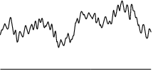
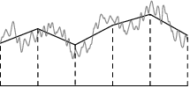
The notation chosen to represent the large scales should be understood as a reference to the finite element mesh size . In practice, scale separation is closely related to the spatial discretization used to solve the problem. This is shown graphically in Figure 1, where the solution along a line is represented. The large scales correspond to the part of the solution that can be described using the finite element interpolation, while the small scales represent fine features of the solution that cannot be reproduced due to the limitations of the discrete interpolation.

|

|
|
| (a) Continuous domain. | (b) Discrete domain. | (c) Continuous solution. |
|

| |
| (d) Large scale solution. | (e) Small scale solution. | |
| Figure 1: Scale separation. | ||
Once a finite element discretization is defined, the space containing the large scale part of the solution can be identified with that of the admissible finite element functions on the discrete domain. This implies that, instead of working with test functions and solutions defined on infinite-dimensional spaces of functions, we now seek a solution on a restricted, finite-dimensional space of admissible solutions, expressed as
|
|
This in turn allows us to define spaces containing the small scale part of the solution , . The subscale spaces complete the corresponding large scale space, that is, , . As a result, it is clear that small scale spaces are infinite-dimensional, unlike the large scale ones, and have to be approximated in order to obtain a solution. There is no single way to approximate them and, in fact, the choice of approximate space for the small scales is one of the defining features of the solution method.
We introduce the following compact notation
|
|
Note that we have modified the convective terms in to introduce a convection velocity . This notation is introduced for convenience, as it will allow us to introduce a linearized version of the operator later. Using the compact notation, the weak form of the problem can be expressed as
|
We introduce the scale separation of the problem variables in Eqs. 2.19 and 2.20. Testing against large scale functions, we can write
|
If the small scale test functions are used instead, the following expression is obtained
|
The large scale problem given by Eqs. 2.21 and 2.22 represents the finite element approximation of the original problem, now containing terms that describe the effect of the unresolved scales on the large scale solution. These additional terms cannot be evaluated in practice, as the small scale variables are not known. VMS methods are based on the definition of a model for the small scale variables, which is motivated by the small scale problem of Eqs. 2.23 and 2.24. This model can then be introduced in the large scale equations, closing the problem.
Before we apply this procedure to our problem, it is convenient to operate on Eqs. 2.21 and 2.22 to eliminate all spatial derivatives of small scale functions, obtaining an expression that depends on and , which will be modeled, but not on their gradients, which will remain unknown. We start by separating the terms involving the large and small scale parts of the solution
|
|
Integrating by parts within each element in the mesh, differential operators acting on and are moved to the test functions. To do so, we introduce the notation of to refer to the part of the problem domain corresponding to element and to denote its boundary.
|
In the present work, the boundary integrals appearing in Eqs. 2.27 and 2.28 will be neglected. This is common in VMS formulations, and can be understood as assuming that the small scale unknowns vanish on element boundaries.
In the following we express this element-by-element integration using the notation
|
|
2.3.2 Small scale equation
Now the question is to define a model for and that can be used to evaluate the domain integrals in Eqs. 2.27 and 2.28. To do this, we start from the small scale problem, given by Eqs. 2.23 and 2.24, which can be developed to read
|
Again, it is convenient to use integration by parts element-by-element on some of the terms in the momentum equation, obtaining the expression
|
|
(2.32) |
Note that the elemental boundary integrals in Eq. 2.32 vanish over internal boundaries because they involve either the exact traction or the exact velocity over the boundary, which are both continuous. Similarly, they cancel out with the corresponding traction in the Neumann boundary. As a result, all boundary terms in Eq. 2.32 can be eliminated in the following.
Rearranging terms in Eqs. 2.32 and 2.31 to separate large and small scale unknowns we can write
|
Eqs. 2.35 and 2.36 can be understood as the projection onto the space of small scales of a differential equation, in the same sense as Eqs. 2.10 and 2.11 represent the projection onto of the Navier-Stokes equations. Moreover, observing the right hand side terms of Eq. 2.35, we can see that it represents the projection of the strong-form linear momentum equation applied to the large scale part of the solution ,. The same can be said about the right hand side of Eq. 2.35, which corresponds to the mass conservation equation applied to the large scale velocity.
Denoting the projection onto the small scale spaces , with and , respectively, Eqs. 2.35 and 2.36 equation can be stated as
|
Since Eqs. 2.39 and 2.40 must hold for all admissible small-scale test functions and , they are equivalent to imposing that the small scale variables , verify the following problem in each element :
|
where and represent the residual form of the Navier-Stokes equations applied to the large scale variables
|
and and are chosen to enforce that right hand sides of Eqs. 2.41 and 2.42 belong to the corresponding small scale space.
As mentioned in the previous pages, the small scale spaces are infinite-dimensional and have to be approximated before the problem given by Eqs. 2.41 and 2.42 can be solved. In practice, the definition of an approximate small scale space corresponds to a choice of projectors and . The most straightforward possibility is to use the entire residual (without projecting to a particular space), which corresponds to considering operators , equal to the identity function or, equivalently, and . This formulation gives rise to the algebraic sub-grid scale (ASGS) method [39].
Another well-known choice consists in taking a small scale space that is orthogonal to the large scale space. If and are the projection onto the large scale spaces and respectively, then the projections in Eqs. 2.39 and 2.40 are defined as , . In this case, and are chosen to subtract from the equation the part of the residuals that belongs to the finite element space, that is,
|
This choice leads to the orthogonal sub-scale (OSS) method, presented in [40,30].
Note that, due to their definition, and belong to the space of finite element functions and can be constructed from their values on mesh nodes using standard finite element interpolation functions.
A second important remark is that the calculation of and requires knowledge of the finite element solutions , and, as a result, it is coupled to the solution of the stabilized Navier-Stokes equations. In principle, this would double the number of nodal degrees of freedom of the problem. However, in practice, given that the Navier-Stokes problem is non-linear and has to be solved iteratively anyway, the projection problem can be implemented in an staggered way, updating the projections after each non-linear Navier-Stokes iteration.
The problem for the small scales, given by Eqs. 2.41 and 2.42, is not usually solved. Instead, it is approximated by an expression of the form
|
|
(2.47) |
where second order tensor and the scalar , known as stabilization parameters, are algorithmic quantities that have to be defined to complete the method.
A motivation for this expression can be found in [30], where the parameters in Eq. 2.47 are designed to ensure that the norm of the modeled subscale variables is the same as that of the exact small scale values. A different justification, based on the approximation of the Green's function of the small scale problem, is provided in [16,21].
2.3.3 Quasi-static small scale models
While Eq. 2.47 represents the complete small scale model derived from the dynamic Navier-Stokes equations, many VMS formulations that can be found in the literature (see for example [39,41,21]) neglect the time variation of the velocity small scale model and define the small scales as
|
|
(2.48) |
This choice corresponds to the assumption that the velocity small scales adapt automatically to the large scale residual. Following the nomenclature of [39], we refer to models based on Eq. 2.48 as quasi-static subscales, as opposed to dynamic subscale models, based on Eq. 2.47.
To complete the formulation, a definition for the stabilization parameters is needed. We follow the approach of [39], where the velocity stabilization parameter is taken to be a diagonal matrix and
|
where is a characteristic length of the element and , are constants, which, for linear finite elements, are usually defined as , (this is the case for example in [42] or [34]). However, the studies presented in [31] for a turbulent channel flow in the low Mach number regime suggest that the choice of values for these parameters can have an impact on the solution. Based on the results presented in that reference and in [27], we have adopted , for our tests.
As pointed out in [20], the use of quasi-static subscales leaves open the possibility of instabilities appearing for small time steps once the problem is discretized in time. The same instability is studied in [43] for the Stokes problem, where it is shown that it can be neutralized if the stabilization parameter satisfies the condition
|
|
(2.51) |
where is the time step and is a constant. To avoid this instability, the stabilization parameter can be replaced by the modified expression
|
|
(2.52) |
although, as remarked in [20], this introduces a dependency of the solution on the time step, even for problems that result in a stationary solution.
2.3.4 Dynamic small-scale models
If, instead of the quasi-static model of Eq. 2.48, we use the dynamic model of 2.47, the time evolution of the velocity small scale has to be taken into account. This was achieved in [30,20] by introducing a time discretization for the small scale acceleration, resulting in the time-discrete small scale model
|
|
(2.53) |
Taking , which corresponds to a backward Euler time scheme, we can write a closed expression for the small scale velocity, given by
|
|
(2.54) |
As remarked in [20], the effective stabilization parameter in Eq. 2.54 is
|
|
(2.55) |
which is precisely the expression introduced as in Eq. 2.52 and prevents the apparition of instabilities due to small time steps. However, unlike in quasi-static approximations, when the problem has a stationary solution, the dependency on the time step is eliminated as, in that case, and the quasi-static model of Eq. 2.48 is recovered.
From the point of view of its implementation, the main difference between the quasi-static model of Eq. 2.48 and Eq. 2.54 is that the latter introduces the old value of the velocity small scale in the model. This means that has to be tracked in time. In practice, this implies evaluating and storing historical values for on the integration points of the finite element mesh.
2.3.5 Complete equations
Once the small scale model is defined, it can be introduced in the large scale equations, given by Eqs. 2.27 and 2.28. The most general formulation that can be obtained from the material presented in the previous section is given by
Momentum equation
|
|
(2.56) |
Mass conservation
|
|
(2.57) |
The first two rows of Eq. 2.56, in combination with its right hand side, constitute the standard Galerkin discretization of the momentum equation. The terms in the third row model the effect of the velocity small scale fluctuations and the velocity small scale itself, respectively, on the large scale equations, while the first term in the last row of Eq. 2.56 represents the effect of pressure small scales.
Analogously, the left hand side of Eq. 2.57 represents the Galerkin weak form of the incompressibility equation, while its right hand side models the effect of the small scales in mass conservation.
While Eqs. 2.56 and 2.57 represent a general VMS formulation, they can be particularized to recover several well-known stabilized methods:
D-ASGS Dynamic algebraic sub-grid scales [20]. The algebraic approximation to the small scales is characterized by using an identity projector to define the small scale space, which implies that the projection terms and are zero. zero.
Q-ASGS Quasi-static algebraic sub-grid scales [39]. A quasi-static approximation to the small scales can be recovered by neglecting all terms involving either the small scale acceleration or the old small-scale velocities and replacing by the static stabilization parameter . Additionally, as the small scales are algebraic, projection terms and are also zero.
D-OSS Dynamic orthogonal subgrid-scales [30,20]. If the small scale space is assumed to be orthogonal to the large scale space, the integral involving and is zero, as it corresponds to the product of two terms belonging to orthogonal spaces.
Q-OSS Quasi-static orthogonal subgrid-scales [30] can be recovered from the original expression by neglecting all terms involving or and replacing by .
For OSS formulations, the projections and are defined as the projections of the momentum and mass residuals, respectively, onto the finite element mesh. Applying this definition, they can be obtained as the solution of the projection problem
|
The only question that remains to close the formulation is to provide a formal definition for the auxiliary convection velocity , something that we have been deliberately avoiding up to this point. This variable was introduced to linearize the convective term, and in practice we can identify it with the last known value of velocity, which corresponds to a Picard linearization of the momentum equation. However, in a context of scale separation, should we use the large scale velocity or the full velocity ?
Both choices result in viable stabilized formulations. The classical approach is to use only the large scale velocity , as it corresponds to the finite element solution. However, from a theoretical point of view, using the full velocity has interesting implications for turbulence modeling, which will be the main focus of Section 2.4.
2.4 VMS methods and Large Eddy Simulation
The concept of scale separation introduced by VMS formulations has some parallels with Large Eddy Simulation (LES) methods for the simulation of turbulent flows. LES turbulence models are also based on separating large and small motions in the flow, but in the LES approach this is is typically achieved through the introduction a filtering operation [2], defined as
|
|
(2.61) |
where is a filter function defined on the interval and is known as the filter width.
Applying a filter function to Eqs. 2.3 and 2.4 allows us to write the filtered Navier-Stokes equations, given by
|
where we have used the conservative form of the convective term and is the subgrid stress tensor, defined as
|
|
(2.64) |
The subgrid stress tensor represents the effect of the small scale motions on the large scale part of the solution and and is an unknown, since the quantity cannot be obtained from the filtered velocity . This means that Eqs. 2.62 and 2.63 do not represent a closed expression. However, if the filter width is chosen small enough that the filtered-out small scale motions can be assumed to lie in the inertial subrange, Kolmogorov's hypotheses [3,4] tell us that they have an isotropic, universal (problem-independent) behavior. LES methods use this approach to motivate a model for and justify its introduction in the filtered equations, closing the formulation.
Introducing the subgrid velocity , the subgrid stress tensor can be rewritten using the Leonard decomposition as
|
|
(2.65) |
where each of the individual terms is defined as:
|
The different terms in Eqs. 2.66–2.68 represent subgrid stresses due to the interaction between resolved motions (Leonard stresses), to the interaction between large and unresolved motions (cross stresses) and to the effect of completely unresolved motions (Reynolds stresses).
Like filtering in LES methods, scale separation in VMS formulations introduces a clear division between the resolved and unresolved parts of the solution, which in this case is achieved through the projection to the finite element mesh. This projection to the mesh was introduced in writing the large scale equation, given by Eqs. 2.21 and 2.22, which is rewritten using the conservative form of the convective term to be consistent with the LES expression above, obtaining
|
where boundary terms and terms related to the trace of the viscous stresses have been omitted for clarity and the full velocity has been used for both arguments of the convective term.
An analogy can be established between Eqs. 2.62 and 2.63, which represent the filtered Navier-Stokes equations and Eqs. 2.69 and 2.70, which expresses the projection of the Navier-Stokes equations to the finite element mesh. This was analyzed in [17,20], where it is remarked that the convective term in Eq. 2.69 can be expanded as
|
|
(2.71) |
The last three terms in Eq. 2.71 can be understood as a variational version of the LES subgrid stress tensor . Ignoring the density, they can be rearranged as
|
|
(2.72) |
where we introduced as a variational analogue of the LES subgrid stress tensor.
Furthermore, can be decomposed into Cross and Reynolds terms as:
|
while an analogue of the Leonard stress, representing the contribution of the resolved velocities to the unresolved stresses, appears in the corresponding small scale equation
|
|
(2.75) |
Assuming that the grid size is small enough for the unresolved scales to be in the inertial subrange, we can observe that scale separation and projection to the finite element mesh play a similar role to that of filtering in classical LES methods. It is worth mentioning that the concept of mesh-induced filtering has also been explored by the LES community, where it is known as implicit filtering. This is the basis of the Monotone Integrated Large-Eddy Simulation (MILES) approach of Boris et al. [44], where the authors propose not using an explicit model for the subgrid stresses and relying instead on a specially designed numerical method to introduce the correct dissipation for a given mesh resolution.
A different approach to VMS-based LES, which will only be mentioned here, is based on a three–level scale separation (see for example [41,45] or the review of [19]). In such approaches, the small scales are in turn divided into resolved and unresolved small scales. The presence of two levels of small scales can be used to either introduce explicit LES model terms to represent the effect of the unresolved small scales on the problem or to calibrate the amount of dissipation that is introduced using the variational equivalent of the Germano identity [46,47].
2.4.1 The VMS kinetic energy balance
Given that the derivation of VMS formulations is based exclusively in numerical and mathematical arguments, the physical behavior of VMS methods, in terms of reproducing the expected dissipation rates when the small scales are on the inertial subrange, has to be verified. This topic has been studied in [17,18] for the formulation that we are calling Q-ASGS and in [25,26] for OSS-based methods.
An energy balance for the original Navier-Stokes problem can be obtained by taking in the Galerkin weak form of the momentum equation, given by Eq. 2.13, which produces
|
|
(2.76) |
We are interested in obtaining a balance for the kinetic energy, . Using the fact that the full velocity is incompressible and the equality , Eq. 2.76 can be expressed as
|
|
(2.77) |
Eq. 2.77 expresses the balance of total kinetic energy in the domain, and the individual terms represent energy storage () and convection (), the power exerted by external forces () and boundary tensions () and finally viscous dissipation ().
We can obtain an equivalent expression for the kinetic energy contained in the large scale motions, , by taking in Eq. 2.69, in Eq. 2.70 and adding the two equations, obtaining:
|
|
(2.78) |
Note that in Eq. 2.78, and for the remainder of this section, we neglected all boundary integrals to simplify the discussion. This is equivalent to considering a problem with homogeneous Dirichlet boundary conditions.
It is convenient to integrate some of the terms in Eq. 2.78 by parts and rearrange the convective term as follows:
|
|
where we have used the fact that the exact velocity is divergence free.
With this, Eq. 2.78 can be restated as
|
|
(2.79) |
Analogously to the complete energy balance, Eq. 2.79 can be understood as a balance for the kinetic energy associated to large scale motions. Terms and represent the storage and convection of large scale kinetic energy, while term represents the power exerted by the external forces on large scale motions. Term is the viscous dissipation associated to the large scale motions, which can be assumed to be negligible for high Reynolds numbers. The remaining terms represent the transfer of energy between large scale and residual motions, playing an analogous role to production terms in the filtered Navier-Stokes equations.
Finally, we define the residual kinetic energy as . A balance statement for can be obtained by subtracting Eq. 2.79 from Eq. 2.77, which results in
|
|
(2.80) |
In Eq. 2.80, terms and represent the storage and convection of residual kinetic energy, while term represents the power exerted by the external forces on small scale (high wavenumber) motions. The next two terms represent the difference between the total viscous dissipation () and the large scale viscous dissipation (), which was already accounted for in the large scale energy balance of Eq. 2.79. Again, we remark that, in practice, term is expected to be negligible in comparison to term , since viscous dissipation occurs predominantly for motions in the range of the Kolmogorov length scale, while will contain only motions on a much larger scale , lying on the inertial subrange. Finally, terms and represent the production of residual energy due to the pressure and velocity small scales, respectively, and are exactly the same (but now with opposite sign) as the production terms in Eq. 2.79.
Terms and can be modified by noting that, since and ,
|
The last step to obtain the residual kinetic energy balance is to introduce the small scale models for velocity and pressure in Eqs. 2.81 and 2.82. Noting that represents the large scale viscous dissipation and will be negligible for high Reynolds numbers, we can write
|
|
(2.83) |
It is clear that terms and , since the stabilization parameters and were defined as strictly positive. They play the role of energy sinks in the large scale energy balance of Eq. 2.79, while acting as sources on the residual energy equation Eq. 2.80. Term is problem dependent but, if an OSS small scale model is used, it will vanish unless the external forces have a high-frequency (small scale) component. Finally, term only exists for dynamic small scale models. This fact was used in [25] to justify that OSS formulations can account for backscatter (energy transfer from the small scales to the large ones) if a dynamic small scale model is used.
Starting from a similar reasoning, Guasch and Codina [26] use statistical and scaling arguments to show that OSS formulations extract energy from the large scale equations at the correct rate, provided that some constraints on the behavior of stabilization parameters are respected.
As a final remark on this topic, we compare the large scale energy balance to the filtered energy balance used in filter-based LES formulations. If the kinetic energy associated to the filtered velocity field is defined as , the balance for can be obtained by multiplying the filtered linear momentum equation Eq. 2.62 by and integrating over the fluid domain (see [2]), resulting in
|
|
(2.84) |
where boundary fluxes have been omitted.
We can introduce the definition of the VMS subgrid stress tensor in Eq. 2.78, obtaining
|
|
(2.85) |
where the conservative form of the convective term has been used. Rearranging some terms, Eq. 2.85 can be rewritten as
|
|
(2.86) |
where we have used the fact that is a symmetric tensor to write . Terms to have an analogous interpretation to their counterparts in Eq. 2.79, but here we have obtained an additional term, , which explicitly represents the contribution of the residual subgrid stresses in the energy transfer. Comparing Eq. 2.86 to Eq. 2.84, we see that both LES and VMS approaches extract energy from the large scale problem through subgrid stresses, but that the variational approach gives rise to two additional energy transfer mechanisms, represented by terms and , compared to filter-based LES.
2.5 Discrete problem
To obtain a finite element solver based on the VMS formulation introduced in Section 2.3 we need to discretize the simulation domain, both in space and in time, and linearize the problem to obtain a system of equations that can be inverted using a linear solver. We start by introducing a finite element partition for the problem domain . Given the discrete domain , the large scale interpolation spaces and can be identified with the standard finite element interpolation functions and the large scale part of the solution, and , can be represented using a finite element interpolation as
|
|
(2.87) |
where represents the number of nodes in the finite element mesh, and are the nodal values of the large scale variables and respectively, represents the standard finite element basis function associated to node and its counterpart for vectorial variables, given by
|
|
Additionally, we introduce the following notation for the gradient and divergence of the finite element shape functions, which will be used to write the discrete form of the differential operators involved in the problem
|
|
(2.88) |
We also introduce the following operator to describe convection
|
|
(2.89) |
and the strain rate matrix, which will be used to write the discrete version of the viscous term
|
|
(2.90) |
Additionally, we define , and as the vectors of nodal values of large scale velocity , acceleration and pressure , respectively.
We introduce the finite element discretization of Eq. 2.87 in the variational formulation given by Eqs. 2.56 and 2.57 to obtain the matrix form of the problem. We will analyze the resulting expression for each of the variants we are considering in turn.
Note that in the present work we use linear finite elements, which can not be used to write second derivatives of the variables or test functions. As a result, terms involving in Eq. 2.56 or the strong-form viscous term that appears in the residual introduced in Eq. 2.43 will be neglected in the discrete form. It must be remarked that all terms lost in this way are related to viscous stresses, which should be small in turbulent flow problems.
2.5.1 Quasi-static ASGS formulation
The quasi-static ASGS formulation is in some sense the classical VMS formulation for the Navier-Stokes equations. It is also relatively simple, as it does not involve dynamic terms or projections, so we will present it first.
Starting from Eqs. 2.56 and 2.57, we can neglect all terms involving the projections or . As the small scales are described using Eq. 2.48, terms involving or in these equations can be ignored and the momentum stabilization parameter is , given by Eq. 2.49. After these simplifications, we introduce the finite element interpolation of Eq. 2.87 to describe the problem variables , . Testing against each nodal basis function in turn we obtain a system of equations that can be expressed in matrix form as
|
|
(2.91) |
|
|
(2.92) |
Again, we have used a generic convection velocity in all terms that have a non-linear dependence of velocity. Doing so, we leave open the possibility of using either the full velocity or the only large scale part . Note that, for linear finite elements, the latter choice is equivalent to the Galerkin-Least Squares (GLS) method [37].
The different matrices in Eqs. 2.91 and 2.92 represent the discrete version of the operators in Eqs. 2.56 and 2.57 and can be built from the assembly of elemental contributions. In general, matrix is constructed by the finite element assembly of elemental matrices of the form . For a finite element with nodes, can be defined using blocks , where and are local node indices. Using this notation, the standard Galerkin terms in the variational form of the problem give rise to the following elemental matrices
|
When defining the viscous matrix in Eq. 2.96 we introduced the constitutive matrix , which is given by
|
|
(2.101) |
In the same way, the stabilization terms in the Q-ASGS give rise to additional elemental matrices, expressed here as
|
2.5.2 Quasi-static OSS formulation
The next variant to be presented is the quasi-static OSS formulation. Compared to the Q-ASGS formulation, OSS is characterized by the inclusion of the projections and , which make the small scale variables orthogonal to the large scale unknowns and should reduce the overall amount of numerical diffusion introduced in the problem. As in the previous case, we leave open the possibility of using either or for convection and the corresponding stabilization terms. The matrix form of the Q-OSS formulation can be expressed as
|
|
(2.111) |
|
|
(2.112) |
where the following three new terms terms, involving the projections, have been introduced:
|
The calculation of the projections involves the solution of an additional problem, given by Eqs. 2.59 and 2.60, which can be expressed in discrete form as
|
where and represent the vectors of nodal values of and respectively and the remaining matrices and vectors are given by
|
Eqs. 2.116 and 2.117 represent an additional problem, coupled to Eqs 2.111 and 2.112, which effectively doubles the number of nodal unknowns in the problem. However, since the system matrices for the projection problem, defined by Eqs. 2.118 and 2.119, are effectively mass matrices, they can be replaced by the corresponding diagonal mass matrix, which allows us to obtain an approximate projection while avoiding the solution of an additional system.
Note that the matrices and that appear in Eqs. 2.111 and 2.112 are not strictly necessary in OSS based formulations, since they involve the acceleration term that appears in the residual . As noted in [39], the acceleration of the large scale lies in the large scale space and therefore its projection should be itself. As a result, we could neglect both these terms if we also not take into account when evaluating the residual that appears in the projection right hand side vector . However, as the projection is only calculated approximately using a diagonal mass matrix, we have found it convenient to take these terms into account to improve stability.
2.5.3 Dynamic ASGS formulation
When we use a dynamic approximation for the subscales we have keep track and update the small scale values at each integration point of the mesh. The dynamic small scale velocities are defined by the local problem given by Eq. 2.47, which was discretized in time using a Backward Euler time scheme to produce Eq. 2.53. Eq. 2.53 provides an expression for in terms of the residual and the old subscale value . The same Backward Euler scheme can also be used to obtain the following time-discrete expression for the small scale acceleration that appears in the variational form of the problem:
|
|
(2.122) |
Introducing Eq. 2.122 in Eqs. 2.56, we obtain a modified momentum equation with time-discrete small scales, given by
|
|
(2.123) |
where the first term in the third row and the last term on the right hand side appear from the time discretization of the small scale acceleration. Note that all terms without an index are evaluated at the current time step. Although they play no role in ASGS stabilization, we have included the projections and both in Eq. 2.122 and in Eq. 2.123, since the same expressions will be used as a starting point for the dynamic OSS method.
The matrix form of the D-ASGS formulation can be written as
|
|
(2.124) |
|
|
(2.125) |
where we have introduced three new terms on the right hand side involving the old subscale velocity, defined as
|
The terms that arise from the residual in the expression for the small scale acceleration, Eq. 2.122, have been grouped with the corresponding terms in the small scale velocity model, resulting in the following modified stabilization matrices:
|
Note that, unlike in the quasi-static variants, we will only consider using the full velocity to calculate convection for dynamic subscale models.
2.5.4 Dynamic OSS formulation
Finally, we consider the discrete form of the dynamic OSS formulation. Here, contrary to what happened for the D-ASGS formulation, the integral involving and can be eliminated a priori, since it corresponds to the inner product of two terms that belong to orthogonal subspaces. This results in the following matrix formulation:
|
|
(2.133) |
|
|
(2.134) |
where all involved elemental matrices have already been defined in the previous sections.
Note that, as presented for the Q-OSS method, the projections can be solved using a diagonal mass matrix to avoid the solution of an additional system. In this case, there is also the possibility of re-introducing in Eq. 2.133 and 2.134 all terms neglected using an orthogonality argument. To do so, we can replace , , and by their D-ASGS variants, given by Eqs. 2.129–2.132, and subtracting , given by Eq. 2.127, from the right hand side of Eq. 2.133.
2.5.5 Time integration
Regardless of the VMS variant used, once the problem has been discretized in space we obtain an equivalent matrix problem written in terms of the vectors of nodal velocities , pressures and accelerations that can be expressed in general form as
|
|
(2.135) |
We need to introduce a time discretization to write the accelerations in terms the velocities. For this we use the Bossak time integration method (see [48]), which can be described as a member of the generalized- Newmark family of methods with second order accuracy in time. The basic expression of the Newmark method, which is commonly used in solid mechanics problem and written in terms of displacements , velocities and accelerations , is
|
where and are constant parameters. In fluid dynamics it is convenient to rewrite Eq. 2.136 and 2.137 in terms of velocities, as these are the main variables of the problem, resulting in
|
Note that for the velocity based formulation, the displacements only appear in the equation for the new displacements, Eq. 2.139. As a result, both the displacements and the equation to obtain them can be omitted from the problem if we are not interested in their values.
The Bossak method is a generalization of the Newmark method based on introducing a relaxation factor on the acceleration of the system
|
|
(2.140) |
In the Bossak scheme, Eq. 2.138 is used to discretize in time Eq. 2.140, obtaining a system that depends exclusively on velocities, pressures and their spatial gradients. After rearranging some terms, this yields the following time-discrete problem
|
|
(2.141) |
A common choice for the Bossak parameter is , which provides maximum damping of high-frequency oscillations. The Newmark parameters are then chosen to be
|
|
2.5.6 Linearization of the large scale problem
The system described in Eq. 2.141 is non-linear due to the fact that the convective operator, the stabilization parameters, multiple stabilization matrices and the projections all depend on the current value of velocity. We define the residual of the problem at time step after non-linear iterations as
|
|
(2.142) |
The problem now consists in finding , such that . Denoting the increment between two successive iterations with , we use a first order Taylor decomposition to write the zero of Eq. 2.142 as
|
|
(2.143) |
We use Picard iterations, evaluating all matrices and vectors using the last known values of the variables. With this approximation, the system matrix can be written as
|
|
(2.144) |
which means that the linear system of equations that is assembled and solved at each iteration is
|
|
(2.145) |
The problem given by Eq. 2.145 is solved iteratively until the increments of the system variables and or the residual vector are smaller than a predefined tolerance.
2.5.7 Tracking of dynamic subscales
The dynamic small scale problem was discretized in time as Eq. 2.54. Using the full velocity, which is divergence-free, as the convective velocity, and neglecting the viscous stress term, since we are restricting ourselves to linear finite elements, we expand the residual that appears in Eq. 2.54 to obtain the following expression for the small scale velocity:
|
|
(2.146) |
Eq. 2.146 is non-linear, since and both depend on when using . Moreover, it is coupled to the large scale problem through its dependence to and . Similarly, under these assumptions, all terms that depend on or the convection velocity in the large scale problem require a value for to be computed.
To update the value of the small scale velocity we follow the procedure presented in [49,31]. Given known values of the large scale variables, and , we define a target function
|
|
(2.147) |
where we use to denote computed using in Eq. 2.52. We use Newton-Raphson iterations to find a zero of , resulting in
|
|
(2.148) |
The tangent matrix in Eq. 2.148 is computed neglecting the dependence of on , resulting in:
|
|
(2.149) |
With this we can obtain new values for by iteratively solving Eq. 2.148 on each integration point. These can be used to evaluate the values of the convective velocity and in the next iteration of the large scale problem. Similarly, once the large scale problem is converged and we advance to the next time step, Eq. 2.148 is solved once more to obtain the historical values for the small scale.
Note that, for OSS formulations, also depends on the value of , as it represents the projection of . However, this dependence is ignored in the procedure outlined in this section. Taking it into account would imply solving the (global) projection problem, given by Eqs. 2.116 and 2.117, every time a new is obtained.
2.5.8 Finite element solution algorithm
As a summary of the formulation described in this section, we present the full solution procedure for the method as Algorithm 1, including the calculation of nodal projections and tracking of dynamic small scales. For variants where they are not necessary, the corresponding step in the algorithm can be skipped.
|
|
Algorithm. 1 VMS incompressible flow solver. |
This procedure was implemented within the Kratos Multiphysics finite element framework and used to compute all numerical test cases presented in this chapter.
2.6 A new model for the pressure subscale
As described in the previous pages, the VMS formulation provides a stabilized method for the simulation of the Navier-Stokes equations that can be understood as a turbulence model, as justified in Section 2.4. However, its application in numerical simulations shows that the results have a strong dependency on the choice of the stabilization parameters. This is observed both in our own results and in the literature (see for example [31,27], which use basically the same formulation we have described), where it can be observed that the obtained mean velocity profile in the turbulent channel flow changes depending on the precise definition of and on whether the pressure small scale is considered or taken to be zero. In particular, the results in [27] suggest that the optimal choice is problem-dependent, since some test cases provide a better fit to the reference data when the pressure small scale is kept, while in other cases neglecting it yields better results.
All this suggests that the current design for the stabilization parameters does not capture the correct behavior for at least some turbulent flow problems. To further investigate this issue, we study an alternate design for the pressure subscale. We start by motivating the design for the stabilization parameters we have been using up to this point and follow by presenting an alternative.
2.6.1 On the design of the stabilization parameters
Recall that the small scale model is motivated by the small scale problem, given by Eqs. 2.41 and 2.42, repeated here in simplified form as
|
where we have written the convective term in non-conservative form and neglected the trace of . The motivation for the stabilization parameters used up to now, (or ) and , is given in [30], where the response of Eqs. 2.150 and 2.151 to high wave number excitations (which we are most interested in, since the small scales represent highly fluctuating motions) is analysed. In such circumstances, it is observed that
|
The design for given in Eq. 2.49 can be justified by noting that has the same limit behavior as the term in Eq. 2.152 when either the convective or the viscous terms are significantly larger than the other. The justification for is given by introducing Eq. 2.152 in the static version of Eq. 2.150 and taking the divergence. Assuming that and are divergence-free, we obtain
|
|
(2.154) |
or, equivalently,
|
|
(2.155) |
The analysis in [30] also shows that the pressure Laplacian in Eq. 2.155 behaves as , resulting in
|
|
(2.156) |
where the algorithmic constant is adopted by analogy with the viscous term in Eq. 2.152. From this expression, and using Eq. 2.151 the usual formulation for the pressure subscale is recovered
|
|
(2.157) |
Finally, we introduce the scaling argument of Eq. 2.152 back to Eq. 2.150 and obtain
|
|
(2.158) |
The small scale model we have been using up to this point, given by Eq. 2.47, is then recovered by neglecting , which effectively uncouples the small scale velocity and pressure models.
2.6.2 Alternative design for the pressure subscale
As an alternative, we propose a formulation which keeps the pressure gradient in Eq. 2.150 and uses it to introduce the pressure subscale. We start by analyzing how keeping the small scale pressure gradient modifies the large scale problem. Retaining means that Eq. 2.158 can be rewritten as
|
|
(2.159) |
hence the corresponding time-discrete small scale velocity model is
|
|
(2.160) |
Introducing Eq. 2.160 as our small scale model in Eqs. 2.56 and 2.57 we can obtain the full problem corresponding to this formulation. The resulting formulation, particularized for the quasi-static subscale case to reduce the number of terms involved, can be expressed as
|
|
(2.161) |
|
|
(2.162) |
where the terms including contributions from have been underlined. Note that the same reasoning could be applied to dynamic subscale formulations.
If we could define an approximate space for and discretize Eqs. 2.161 and 2.162, we would be able to write a matrix problem of the type
|
|
(2.163) |
where matrix and vector represent the matrix problem resulting from either Eqs. 2.91 and 2.92 for the Q-ASGS formulation or Eqs. 2.111 and 2.112 for the Q-OSS formulation, and are the (large scale) vectors of nodal unknowns and results from the contribution of to the underlined terms in Eqs. 2.161 and 2.162. Its precise definition, if was known at the integration points of each element, would be given by
|
We need to provide a model for before we can complete the formulation. To do so, we take a little detour. Consider that the finite element velocity solution , which is not divergence-free, can be decomposed as
|
|
where is a solenoidal field verifying and is a potential field. We identify the pressure small scale with the potential part of the solution , with the goal of obtaining a velocity field that is more divergence-free in some weak sense.
Taking the divergence of and integrating over the element's domain, we write
|
|
(2.166) |
Integrating by parts both sides of Eq. 2.166 we obtain
|
|
(2.167) |
Eq. 2.167 can not be evaluated in practice, since the exact small scale space is infinite-dimensional, but can be estimated using an approximate small scale space. Our proposal is to assume that the the space for the small scale pressure can be approximated by the discontinous version of the large scale space, that is, functions that are linear within each element and discontinuous across element boundaries. The fact that our interpolation functions are discontinuous across element boundaries allows us to write a local problem on each element, given by the discrete form of Eq. 2.167. Denoting with the small scale shape function for node , we can write
|
|
(2.168) |
where and represent the nodal values of and on the element and the matrices are build from nodal contributions of the type
|
Note that, for the shape functions we are proposing, on a given element, is equivalent to the elemental discrete divergence matrix of the large scale problem, given by Eq. 2.98.
Matrix represents the discrete form of a Laplacian problem and can be explicitly inverted on each element if additional restrictions are imposed on the variable . In our tests, we have imposed that is zero on average over the element, which allows us to write
|
|
(2.171) |
Going back to the enhanced matrix problem of Eq. 2.163, the small scale shape functions can be used to rewrite the additional terms and in terms of the nodal vector
|
|
(2.172) |
where we introduced the new finite element matrices
|
Finally, we substitute Eq. 2.171 in Eq. 2.172, eliminating the additional variables from the problem algebraically
|
|
(2.175) |
To complete the formulation we would need to define a model for (as opposed to its gradient), which also appears in Eq. 2.161. However, since we imposed that is zero on average in each element to ensure that can be inverted and we are using linear shape elements (which means that is constant within each element), it can be verified that, for the proposed formulation,
|
|
(2.176) |
where is a constant that depends on the shape of the element.
2.7 Application to the turbulent channel flow
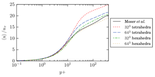
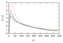
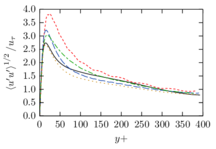
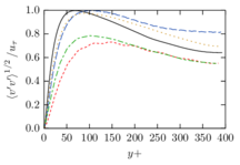
The turbulent channel flow is a classical benchmark for LES formulations, in which a fluid circulates between two parallel walls. In the turbulent regime, the flow is characterized by a transfer of energy from the central regions to the zones close to the wall, achieved through turbulent motions, where it is dissipated through viscous friction. This problem represents a challenge for turbulence models in general and LES methods in particular and is well studied in the literature [50,2]. For moderate Reynolds numbers, it is also within reach of direct numerical simulation (DNS), which means that simulations representing all scales of the flow are available in the literature. In particular, we will use data from the simulations of Moser et al. [51] to validate our results. Note that, while this particular problem could be simulated using DNS, we are not interested in fully resolving all scales of the flow, since we want to study the behavior of the formulation as a LES method.
There is abundant literature validating VMS (and other) formulations on this particular benchmark, which was simulated using dynamic subscales in [27], and in [31] for the low Mach number regime; with and without explicit LES (Smagorinsky) modelling terms in [45], using VMS methods in combination with isogeometric finite element formulations [21,23] and using SUPG stabilization by itself [12] or in combination with the Smagorinsky model [11]. As a result, this example allows us to validate our implementation and test our new approach for the pressure subscale. However, we also note that all previous studies, as far as we know, have used linear hexahedra or higher order interpolations. In contrast with previous studies, we want to use this example to compare the results obtained with tetrahedral and hexahedral elements since, while hexahedra provide a richer interpolation, tetrahedra are in many cases the only practical choice to discretize complex geometries, and we want to quantify the impact of using tetrahedral interpolation on the solution.
The simulation consists in modeling the flow between two parallel flat plates that are separated a distance . The flow is driven by a pressure gradient applied on the streamwise direction, , which is balanced by the friction produced by the wall, . The wall friction is conventionally expressed as , where is defined as the friction velocity. Given that the forces acting on the problem must be in equilibrium, the pressure gradient and the wall friction are related by the following expressions (see [50] for example):
|
|
The Reynolds number can be given in terms of the friction velocity and the channel width as
|
|
which is denoted by to distinguish it from the bulk Reynolds number, computed using the average streamwise velocity of the flow (see [2]).
For our tests, the Reynolds number is set to , which can be obtained by setting the problem parameters to
|
|
The problem domain is restricted to in the stream-wise, wall-normal and cross-stream directions respectively, which corresponds to the domain used in [21]. Zero Dirichlet conditions are applied on the solid walls and periodic boundary conditions are used for the remaining sides.
2.7.1 Effect of the simulation mesh
For a first set of tests, we simulate the problem using regular hexahedral and tetrahedral meshes. The meshes are defined by introducing 32 or 64 divisions on each coordinate direction, which immediately defines a mesh of or hexahedra. Tetrahedral meshes can then be obtained by splitting each hexahedra into six tetrahedra. The mesh nodes are evenly distributed on the streamwise and cross-stream directions while, on the wall normal direction, they are distributed according to the law
|
|
where is the number of divisions on the direction and . The weight is chosen as for and for so that the first node has a dimensionless distance to the wall .
The flow is simulated using a time step of , starting from the average flow profile plus a random disturbance and let to evolve until a statistically steady regime is obtained. Discarding this initial transient phase, statistics are recorded on the integration points of the mesh using the method described in Chapter 4. Since the problem is statistically homogeneous, statistics can be obtained by ensemble-averaging data on planes corresponding to the same wall distance. This averaging of spatial and time data is known as Reynolds averaging in the context of turbulence modeling. We denote the (Reynolds) average value of a quantity as and the fluctuation as . A snapshot of the obtained instantaneous streamwise velocity and the distribution of the elements close to the wall can be observed in Fig. 2 for a tetrahedral mesh and in Fig. 3 for a hexahedral mesh.
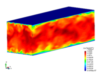
|
|
| (a) Instantaneous streamwise velocity. | (b) Detail of the mesh. |
| Figure 2: Channel flow – Solution and mesh for the tetrahedra simulation. | |
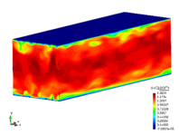
|
|
| (a) Instantaneous streamwise velocity. | (b) Detail of the mesh. |
| Figure 3: Channel flow – Solution and mesh for the hexahedra simulation. | |
We have measured both average velocities and velocity correlations, all of which can be compared to the DNS data of [51]. Note that the velocity fluctuation correlations can be identified with the turbulence kinetic energy, defined as
|
|
The first set of results has been obtained using the Q-ASGS formulation and the different meshes. The obtained average is compared to the reference data in Fig. 4, while the velocity variances are presented in Fig. 5. Note that the results are expressed in terms of the dimensionless distance to the wall , which is the common practice for this problem. In this notation, corresponds to the wall, while the channel center line is close to .
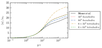
|
| (a) |
| Figure 4: Channel flow – average stream-wise velocity profile obtained for the Q-ASGS formulation, using different meshes. |
Not surprisingly, there is a noticeable change of behavior depending on the element type, with tetrahedra producing generally poorer results for a given mesh size than hexahedra. In particular, it can be observed that the results obtained using tetrahedra are similar to those obtained hexahedra, which suggests that an order of magnitude more tetrahedra are required in this case to obtain a solution comparable to hexahedra.
We can see that we generally overpredict the average streamwise velocity profile, which suggests that we are not dissipating enough linear momentum and stronger velocity gradients are required to achieve an equilibrium solution. Observing the measured velocity variances in Fig. 5, we can see that there are larger than expected velocity fluctuations on the streamwise direction. The dynamic evolution of the solution presents larger divergences from the average value than expected, which again suggests that we are slightly underestimating the dissipation. This situation is reversed on the wall-normal and cross-flow directions, where the obtained dissipation is generally under the DNS measurements.
2.7.2 Influence of the small scale model
The next set of tests is designed to evaluate the effect of the small scale model on the solution. We have chosen the hexahedra mesh and used it to simulate the same case using the different models presented in Section 2.3. Based on the results presented in [27], we have chosen to neglect the pressure small scale for this set of tests, which corresponds to setting , as this was found to result in a better fit to DNS data in that reference. Note that the quasi-static results presented were calculated using only the large scale part of the solution in the convection term, while the full velocity was used for dynamic models.
The average stream-wise velocity profiles for this set of tests are presented Fig. 6, while the measured velocity variances are shown in Fig. 7. The results are in general comparable to those obtained for the same mesh in the previous set of tests and, while the qualitative behavior of the solution is properly captured, the average velocity is slightly overpredicted.
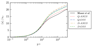
|
| (a) |
| Figure 6: Channel flow – average stream-wise velocity profile obtained on the hexahedra mesh using different small scale models. |
From the obtained results, we can see that the choice of small scale model has an impact on the solution. However, we see that, in our case, the result that produces a closer approximation to the DNS stream-wise velocity profile is the Q-ASGS model, which is the most simplified one from the theoretical point of view.
In terms of the velocity variances, the points made for the previous set of tests still stand. The stream-wise velocity variances are generally overestimated compared to the expected results, while the fluctuations on the other directions are underestimated. Again, the different models introduce some differences in the final solution, with the Q-ASGS and D-OSS variants providing the closest match to DNS data.
2.7.3 Turbulence kinetic energy balance
To obtain a deeper understanding of the results we measured the turbulence kinetic energy balance for the problem. A balance statement for the turbulence kinetic energy can be obtained using a procedure analogous to what presented in Section 2.4 for the residual energy , using Reynolds averaging in place of filtering. Only the final expression is presented here, but the interested reader is directed to [52,2] for detailed proof.
|
|
(2.177) |
where the terms represent, respectively:
- Material variation (storage and advection) of turbulence kinetic energy;
- production due to mean velocity shears;
- turbulent diffusion: transport due to small eddies;
- pressure diffusion: redistribution due to local pressure gradients;
- viscous diffusion and
- viscous dissipation.
For the turbulent channel flow, we have that the average velocity is exclusively in the streamwise () direction and that the flow is homogeneous in the streamwise and cross-stream directions. As a result, all terms involving either , or spatial derivatives along the or directions can be can be neglected from Eq. 2.177, resulting in the simplified expression
|
|
(2.178) |
where the numbered terms have the same interpretation as the corresponding term in Eq. 2.177. Note that, once a statistically steady state has been reached, the storage term in Eq. 2.178 will also be zero, as in equilibrium the power introduced in the system by the external pressure gradient is exactly balanced by wall friction.
The different terms in Eq. 2.178 have been measured in the course of the simulations presented in the previous pages and are presented in graphical form in Figs. 8 to 17, again compared to DNS measurements from [51]. Note that in this case we are only presenting the part of the solution closer to the wall, , as energy transfer phenomena are mostly localized close to the wall for this problem.
The values for term in Eq. 2.178, turbulence kinetic energy production, are plotted in Fig. 8 for the different meshes and in Fig. 9 for the different small scale models. The production term measures the generation of small scale motions due to the shear of the average flow and, for this example, is expected to be positive throughout the domain, reaching a peak close to the wall, near . As an aside, the fact that this term is positive means that there is no backscatter in this problem.
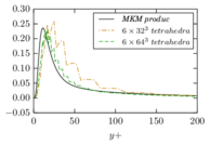
|
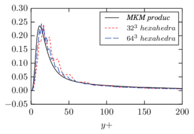
|
| (a) | (b) |
| Figure 8: Channel flow – turbulence kinetic energy production for the Q-ASGS method. | |
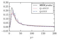
|
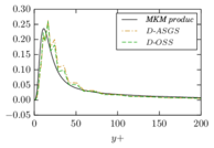
|
| (a) | (b) |
| Figure 9: Channel flow – turbulence kinetic energy production in the hexahedra case for the different small scale models. | |
We observe that our results are in qualitative agreement with DNS data, but tend to predict a peak in production at larger (farther from the wall) than expected. This is most marked for the coarser tetrahedral mesh in Fig. 8a, while hexahedral meshes predict the peak closer to the expected position in general. It is worth noting that the curves obtained from our simulation have a jagged appearance when compared to DNS data. This is due to the choice of linear interpolation functions, which means that the simulated velocity gradient is constant within each finite element. This will also happen in any other results involving spatial gradients of finite element variables.
In terms of the different small scale models tested, we see that the dynamic models in Fig. 9b provide a better match to DNS data than the quasi-static models in Fig. 9a, suggesting that dynamic models do in fact provide a better description of turbulent phenomena compared to the simpler quasi-static models.
As a final remark, note that the hexahedra, Q-ASGS curve in Fig. 8b does not coincide with the Q-ASGS curve in Fig. 9a. The difference between the two curves is due to the pressure small scale, which was considered in the first case and neglected in the latter. It is interesting to observe that retaining it results in a better prediction of the production term, despite the fact that we saw in the previous pages that neglecting the pressure small scale results in a closer approximation of the average stream-wise velocity.
Term of Eq. 2.178, which corresponds to turbulent diffusion, is presented in Fig. 10 for the different meshes. Turbulent diffusion is expected to transfer energy from the intermediate region of the channel towards the wall, which means that it will act as a source of turbulence kinetic energy (positive values) close to the wall and as a drain (negative values) at large . We see that our results follow the expected distribution of values, closer when using hexahedral meshes. However, it is interesting to note that the positive peak, near , is underestimated in the finer simulations.
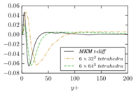
|
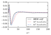
|
| (a) | (b) |
| Figure 10: Channel flow – turbulent diffusion for the Q-ASGS method. | |
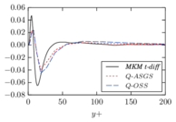
|
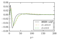
|
| (a) | (b) |
| Figure 11: Channel flow – turbulent diffusion in the hexahedra case for the different small scale models. | |
The measured turbulent diffusion for the different small scale models is presented in Fig. 11 and shows the same type of dependence on the model that we observed for the production term. Again, dynamic subscales provide a better approximation to DNS data than quasi-static ones and, comparing Fig. 10b to Fig. 11a, using the pressure small scale in the Q-ASGS case provides a closer match than neglecting it.
Turning our attention to term , which represents pressure diffusion, we provide the results corresponding to different meshes in Fig. 12 and to the different small scale models in Fig. 13. This term corresponds to the relation between local pressure and velocity fluctuations and it has a qualitative behavior that is similar to that of turbulent diffusion, transporting energy closer to the wall, but a smaller magnitude in general. As in the previous term, we can observe that the obtained results tend to underestimate sharp peaks. However, in this case, we detect an unexpected behavior close to the wall for the finest hexahedral mesh, as can be seen in Fig. 12b, where the hexahedra curve shows a negative peak close to the wall. As a possible interpretation of this result, we note that elements are highly stretched in that region and that we are using an average element size to define our stabilization parameter. This could have unexpected effects on the consistency of the stabilization terms and might be adding some error in our calculations.
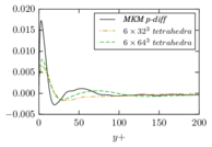
|
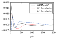
|
| (a) | (b) |
| Figure 12: Channel flow – pressure diffusion for the Q-ASGS method. | |
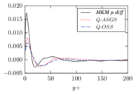
|
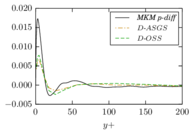
|
| (a) | (b) |
| Figure 13: Channel flow – pressure diffusion in the hexahedra case for the different small scale models. | |
The results obtained for term , representing viscous diffusion, are presented in Fig. 14 for the different meshes used and in Fig. 15 for the different small scale models. As the other two diffusive terms, viscous diffusion transports energy towards the wall but, compared to the the previous terms, it acts closer to the wall in general. This is consistent with the fact that viscous effects are predominant only in the smallest motions, which, for the turbulent channel flow, are significant only at a very close distance from the wall.
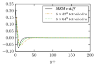
|
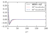
|
| (a) | (b) |
| Figure 14: Channel flow – viscous diffusion for the Q-ASGS method. | |
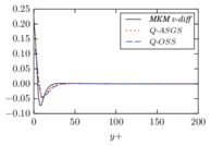
|
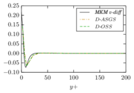
|
| (a) | (b) |
| Figure 15: Channel flow – viscous diffusion in the hexahedra case for the different small scale models. | |
The final term in Eq. 2.178, term , corresponds to viscous dissipation of turbulence kinetic energy. This term should be negative throughout the domain, as viscous dissipation is the only energy sink available in the problem, which can be verified in Fig. 16 for the different meshes and Fig. 17 for the different small scale models.
Viscous dissipation should predominantly occur close to the wall, where the smallest motions are concentrated, and we notice that our results follow this general trend, in agreement with DNS data. However, all our curves indicate a smaller (closer to zero) dissipation for any given distance to the wall, which seems to be generally in line with our interpretation of the average velocity results, indicating that dissipation is generally lower than expected.
In terms of the comparison between the different methods, the results obtained for dissipation are in agreement with the general trend observed for the previous terms. We notice that dynamic models, as shown in Fig. 17b, provide results that are slightly closer to DNS measurements than quasi-static models, which in this case is clear in the small step displayed by the different curves close to the wall, and that the Q-ASGS results in Fig. 16b, obtained using the pressure subscale, are slightly better than those in Fig 17a, obtained by neglecting it.
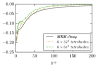
|
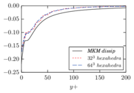
|
| (a) | (b) |
| Figure 16: Channel flow – turbulence kinetic energy dissipation for the Q-ASGS method. | |
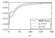
|
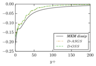
|
| (a) | (b) |
| Figure 17: Channel flow – turbulence kinetic energy dissipation in the hexahedra case for the different small scale models. | |
2.7.4 Effect of the proposed pressure subscale model
As a final test, we simulated the same problem using the alternative model for the pressure subscale proposed in Section 2.6 and the coarser tetrahedral grid, comprising tetrahedra. We present the results in terms of the average stream-wise velocity profile and velocity variances in Fig. 18, where we compare them to DNS data and to the regular Q-ASGS formulation, either retaining () or neglecting () the pressure small scale. We observe that both neglecting the pressure small scale and using the proposed model result in a much closer agreement to DNS data compared to retaining . This allows us to obtain results that are much closer to those obtained using hexahedra, which were presented in Fig. 4, while using a tetrahedral mesh.
2.8 Concluding remarks
We devoted the present chapter to introduce VMS stabilized formulations for the incompressible Navier-Stokes equations and to expose the arguments that have been used to relate them to LES methods for turbulence modeling. Besides the classical VMS approach, we have discussed dynamic subscale models and the possibility of using the last known value of the complete velocity as the linearized advective velocity on the convective term. These two modifications to the basic formulation allow us to provide a stronger theoretical justification to the use of VMS methods as a type of turbulence modeling, similar to LES but using a projection to the mesh instead of spatial filtering to introduce scale separation. We have implemented a finite element solver based on dynamic subscale formulations and used it to simulate the well-known benchmark of the turbulent channel flow at .
We have investigated the effect of using either tetrahedral or hexahedral meshes for the simulation and the use of different small scale models. Motivated by results found on the literature, we decided to neglect the pressure subscale in some of the tests, in the hope of obtaining more accurate solutions. While it is true that neglecting the small scale pressure results in a better agreement to DNS data in terms of the average stream-wise velocity in the single direct comparison we have for this (the Q-ASGS model), we have also found that this choice results in a poorer prediction of the turbulence kinetic energy balance. We do not have a definitive answer to this apparent contradiction, but one possible explanation could be that the small scale pressure introduces an unexpected energy transfer mechanism, which we do not detect in our balance, since we are only measuring the (large scale part of) the terms in Eq. 2.178. Obviously, more tests are required before a definitive answer can be provided, and the first step would be repeating the analysis presented in Section 2.7 but now without neglecting the pressure subscale and measuring not only the large scale part of the energy balance, but also the contributions of the small scale velocities to the terms in Eq. 2.178.
This dependence of the results on the pressure small scale also motivated us to propose a new model for the pressure small scales, which we based on strengthening the enforcement of the incompressibility of the velocity solution via the use of an approximate interpolation space for the small scale pressure. While this new formulation produces improved results when compared to the classical approach on a tetrahedral mesh, we want to remark that the effect of the pressure small scale term seems to be problem-dependent (this can be seen for example in [27]), which means that this should be understood as the starting point of a wider investigation and not a definitive result.
In the same sense, in proposing the formulation we have made some arbitrary decisions, such as the choice of a discontinuous linear interpolation space or the zero-average condition used to invert the Laplacian in Eq. 2.171. These are by no means the only possibilities, and it would be interesting to know the impact of this choice compared to other alternatives.
3 A Finite Calculus stabilized finite element formulation for turbulent flows
3.1 Introduction
In the present chapter we introduce a new stabilized finite element formulation for the simulation of incompressible flow problems based on the Finite Calculus (FIC) approach [53,54]. FIC is a general framework for the development of stabilized formulations, based on writing the balance equations of the problem for an arbitrarily small domain, instead of the usual point-wise partial differential equation (PDE). This results in a modified strong-form equation with additional terms that, once the problem is rewritten as a variational equation, have a stabilizing effect on the numerical formulation.
The FIC approach has been applied to incompressible flows at a range of Reynolds numbers in the past [14,13,55], but in the present document we intend to investigate the behavior of the formulation as an alternative to large eddy simulation (LES) in a finite element context, as we did for Variational Multiscale (VMS) based formulations in the previous chapter.
The main new feature of the FIC formulation presented here, compared to previous approaches, is the addition of a new dissipative term based on the velocity gradients. This term has an effect on the total dissipation introduced by the numerical formulation and will be shown to improve the accuracy of the solution for the turbulent flow examples considered.
We will start by presenting the general FIC approach in Section 3.2. This approach will be used to obtain a stabilized expression for the linear momentum balance in Section 3.3 and a stabilized continuity equation in Section 3.4. These two expressions will be combined to obtain a discrete formulation in Section 3.5. The presented formulation will then be used to simulate a turbulent channel in Section 3.6, the flow past a cylinder in Section 3.7 and a solar collector in Section 3.8. Finally, some concluding remarks are presented in Section 3.9.
3.2 FIC formulation
Although our end goal is to apply the FIC formulation to the full Navier-Stokes equations, it is convenient to introduce it first on a simpler problem. We present the first order FIC balance following the approach of [56], by applying it to the advection-diffusion equation.

|
| Figure 19: Fluxes in a domain. |
Consider a scalar quantity advected with a velocity through the domain shown in Fig. 19. The domain has a total length and diffusivity coefficient . The distribution of will be the solution of the convection-diffusion equation
|
|
(3.179) |
Furthermore, we can define the flux passing through a point on the domain as
|
|
(3.180) |
Consider the flux through the boundary of the domain. Given that the fluxes , entering and exiting it through its extremes must be in equilibrium, we can write
|
|
(3.181) |
The basic premise of the FIC approach is to write Eq. 3.181 in terms of the flux through an arbitrary point that lies in the interior of the domain. If the fluxes at and are expressed as a Taylor series expansion of the flux at , we can state
|
|
If we introduce these definitions in Eq. 3.181 we can rearrange the resulting expression to obtain
|
|
(3.182) |
where we used that . In FIC formulations, the quantity is defined as the characteristic length of the problem. Introducing the definition of the flux in Eq. 3.182 and neglecting third order derivatives we recover the expression
|
|
(3.183) |
where we have neglected the spatial variation of and .
As the position of point in the balance domain of Fig. 19 is arbitrary, Eq. 3.179 holds for any point within the analysis domain. Comparing Eq. 3.183 to the pointwise balance equation Eq. 3.179, we see that, by enforcing the balance of fluxes on the finite-sized domain , we introduce a modified diffusivity, which acts as an additional source of numerical diffusion as long as the characteristic size is chosen such that . This has a stabilizing effect on the resulting finite element formulation. Note that, in contrast to most stabilization frameworks (such as the VMS formulation presented in the previous chapter), the stabilizing terms appear as a result of a modification of the original PDE and not from a manipulation of the variational form.
The procedure used here to obtain the FIC formulation for the advection-diffusion equation can be extended to other problems and multiple dimensions, and is known in the FIC context as first order FIC balance in space. Defining the residual form of our problem as
|
|
(3.184) |
we can rearrange the terms in Eq. 3.183 as
|
|
(3.185) |
where we are once more neglecting the spatial variation of and and all third-order derivatives.
The same approach can be extended to multiple dimensions [54]. The vector form of the FIC equation reads
|
|
(3.186) |
where represents the characteristic length in the -th coordinate direction. We will use the notation to denote the vector of characteristic lengths in the different coordinate directions.
This procedure can be directly applied to the momentum equation. We will follow a slightly different approach for the mass conservation equation, originally introduced in [57], which retains higher order terms in the FIC balance to obtain a second order expression.
3.3 Stabilized momentum equation
We present first the FIC stabilized form of the momentum equation. This equation was already introduced in the previous pages, but is stated in Eq. 3.187 for reference. Note that, as we did for the VMS formulation in Chapter 2, we follow the approach of [34] and use the skew-symmetric form of the convective term.
|
|
(3.187) |
For a Newtonian fluid, the stress tensor can be expressed in terms of the rate of strain tensor as
|
We can follow the procedure outlined in the previous section to develop FIC-based stabilized form of the momentum equation. We introduce Eq. 3.188 in Eq. 3.187 and rewrite it in residual form as
|
|
(3.190) |
Expressing the balance of linear momentum along each spatial direction and following the argument of the previous section we can obtain the FIC balance statement for the momentum equation as
|
|
(3.191) |
where represents the length used to write the balance along the -th coordinate direction. Note that, in principle, a different vector of characteristic lengths can be used in the balance equation for each momentum component .
We consider different possibilities to design . The first possibility is to define the characteristic lengths based on the finite element size along the streamlines of the flow, which results in a method similar to the SUPG formulation [36]. A second option is to base the characteristic length on the size of the element along the direction of the gradient of velocity. This acts as a source of additional diffusion, although the resulting formulation is not stable by itself. Finally, we consider the possibility of mixing both approaches by introducing a combination coefficient. Each approach will be presented in succession in the following pages.
3.3.1 Streamline diffusion formulation
Consider a characteristic length vector aligned on the direction of the flow velocity
|
|
(3.192) |
where is the projected length of a given element along the direction of flow, defined by the unit vector . Using this expression, we can rewrite Eq. 3.191 as
|
|
(3.193) |
We can use Eq. 3.193 as the starting point to write a stabilized formulation for the momentum equation. Multiplying by a test function and integrating over the fluid domain we obtain
|
|
(3.194) |
It is convenient to integrate by parts the second term in Eq. 3.194. Note that, as the length will be defined as a constant quantity on each element, the boundary integral that appears should be understood as an integral over elemental boundaries.
|
|
(3.195) |
We have neglected the elemental boundary integrals appearing in Eq. 3.195 in the present work. In practice, this is similar to consider that the small scales vanish over element boundaries on VMS formulations. At this point, we introduce the definition of the residual Eq. 3.190 and its gradient in Eq. 3.195. This gives
|
|
(3.196) |
where represents the -th component of the tractions imposed on the Neumann boundary .
Although Eq. 3.196 was developed using a FIC based approach, the final expression is analogous to a SUPG stabilized formulation, with (which has dimensions of time) playing the role of the SUPG stabilization parameter .
3.3.2 Gradient diffusion formulation
An alternate approach to Eq. 3.192 is to measure the characteristic length in the direction of the gradient of the -th component of velocity, , given by
|
|
(3.197) |
which, as before, can be used to write a FIC balance statement for each component of the momentum equation
|
|
(3.198) |
We can obtain a variational form of the FIC momentum balance equation given by Eq. 3.198 following the same procedure used for the streamline formulation. Multiplying by a test function and integrating over the fluid domain gives
|
The first integral in Eq. 3.200 is identical to the first term of Eq. 3.195 and can be developed as in the previous section. We direct our attention towards the second term in Eq. 3.200, which can be integrated by parts as follows
|
From the three terms in the last equality of Eq. 3.204, only the first one will be kept. The second one is neglected as it involves either spatial derivatives of the characteristic length or second derivatives of velocity. The last term can be transformed into a boundary integral using the divergence theorem, and is dropped for the same reasons we neglected the boundary terms in the streamline formulation. Finally, it is convenient to rewrite the remaining term as
|
|
(3.205) |
If we choose the characteristic length such that , Eq. 3.205 describes the discrete version of a non-isotropic Laplacian, where the diffusivity for each coordinate direction is different. The diffusivity coefficient in this case is proportional to the magnitude of the finite element residual on each coordinate direction and exhibits a similar structure to that of a shock-capturing formulation, such as [58]. The numerical diffusion added on each direction is defined by the tensor :
|
|
(3.206) |
Going back to Eq. 3.200, the weak form for the gradient diffusion formulation reads
|
|
(3.207) |
It must be noted that the formulation of Eq. 3.207 by itself is not sufficient to stabilize convection-dominated flows in general. Therefore, we consider the possibility of combining the present approach with the streamline-based characteristic length.
3.3.3 Combined Approach
As a last possibility, we consider a combined approach including both the stabilizing terms of the streamline-diffusion formulation and the additional diffusion of the gradient formulation. The FIC expression for this case reads
|
|
(3.208) |
where is a combination parameter.
The development of the combined formulation follows the steps of each of its components as shown in the previous pages. Therefore, only the final expression for the weak form, obtained by combining Eq. 3.196 and Eq. 3.207, is given here:
|
|
(3.209) |
with given by Eq. 3.206.
3.3.4 Definition of the stabilization parameters
Eq. 3.209 represents the basic formulation used for the momentum equation in the present chapter. To develop it, we introduced five free parameters (in ): the velocity characteristic length , one gradient characteristic length along each coordinate direction , and the combination parameter , which must be defined before the method can be implemented.
3.3.4.1 Streamline diffusion characteristic length 3.3.4.1 Streamline diffusion characteristic length
h
u
{\displaystyle \mathbf {h {u}} }
The characteristic length for the streamline diffusion terms is defined from the size of the element in the direction of velocity . Defining the unit vector in the direction of velocity as and representing the element edge joining nodes and with the vector , the element length is given by
|
|
(3.210) |

|

|
| Figure 20: Definition of the element lenght for triangles and quadrilaterals. | |
In practice, Eq. 3.210 is evaluated on the integration points of each element. In the case that velocity is (close to) zero on a given point for a given time step, is undefined and this expression can not be used. If this happens, an average element length is used instead. The characteristic length we used in this case will be introduced in Eq. 3.222 for the stabilization of the mass equation.
3.3.4.2 Gradient diffusion characteristic lengths 3.3.4.2 Gradient diffusion characteristic lengths
h
g
i
{\displaystyle \mathbf {h {g {i}}} }
The characteristic element lengths for the gradient term are defined analogously to Eq. 3.210, but using the gradient of the -th component of velocity to define the direction of projection. The characteristic element length to be used for the -th coordinate direction is therefore defined as
|
|
(3.211) |
3.3.4.3 Combination parameter 3.3.4.3 Combination parameter
β
{\displaystyle {\boldsymbol {\beta }}}
In principle, the combination parameter could take any value in the range . The limit case results in the classical FIC formulation for the momentum equation, used for example in [56] or [14]. This formulation is very close to the SUPG stabilization, but uses the stabilization parameter of Eq. 3.194, derived from FIC principles. On the other end of the range, implies using the gradient diffusion term exclusively and results in a formulation that is not numerically stable for convection-dominated problems. In the present work, we have found that values of are typically needed for the problem to be stable for all flow regimes, while values in the range typically give the best results.
In addition to defining the value of as a fixed quantity for the entire simulation, we have also experimented with the possibility of adjusting dynamically using the local features of the flow. In some simulations we have set a local value for depending on the directions of velocity and its gradient:
|
|
(3.212) |
where is a minimum value to prevent the loss of stability if the velocity becomes parallel to in some point. Note that the value of that is obtained using Eq. 3.212 is different for each coordinate direction . This means that, if this expression is used, both the streamline terms and the gradient terms in Eq. 3.209 are non-isotropic.
3.4 Stabilized mass balance equation
In order to obtain a stabilized formulation for the mass balance equation, the approach used in [57,55] will be followed. A similiar approach was also applied in [59] for a quasi-incompressible fluid. We introduce the following notation for the mass balance residual:
|
|
(3.213) |
which can be used to derive the second order FIC balance in space as
|
|
(3.214) |
The expression of second order mass balance was originally used to obtain a stabilized formulation for incompressible flows in [57], where it was derived by expressing the balance of mass within a rectangular domain. In this reference, it is shown that Eq. 3.214 can be obtained by writing the velocities along the boundaries of the rectangle as a Taylor series expansion of the velocity on its center and retaining terms up to third order.
Now the problem consists in obtaining an expression for that is useful for the calculation. To do so, we go back to the momentum balance as stated in Eq. 3.190. Assuming that we are in equilibrium, and therefore , and using the identity
|
|
(3.215) |
we can rearrange the terms in the momentum balance to read
|
|
(3.216) |
Moving all terms involving to the same side of the equality we obtain
|
|
(3.217) |
where we introduced the notation of for the right hand side of Eq. 3.217 for convenience. At this point it is helpful to write the first order FIC balance for the continuity equation
|
|
(3.218) |
and use it to express in terms of its derivative in Eq. 3.217
|
|
(3.219) |
We can introduce Eq. 3.219 in Eq. 3.214 to write
|
|
(3.220) |
Neglecting the spatial variation of the product , we take the coefficient that multiplies out of the derivative, obtaining
|
|
(3.221) |
Eq. 3.221 expresses the basic FIC mass balance statement used in the present work. We will simplify it slightly by using an average characteristic length as done in [59], which allows us to combine the two coefficients in Eq. 3.221 in a single isotropic stabilization parameter
|
|
(3.222) |
where we use the norm of the velocity and the average element length , which is calculated as the square root of the elemental area in or the cubic root of the elemental volume in .
Using we can write the final FIC balance statement for the incompressibility equation as
|
|
(3.223) |
We can multiply Eq. 3.223 by a test function and integrate over the fluid domain to obtain the weak form of the equation
|
|
(3.224) |
It is convenient to integrate by parts the second integral in Eq. 3.224 to reduce the order of the derivatives involved. As in the momentum equation, the boundary terms resulting from this operation are neglected in the present work, obtaining the expression
|
|
(3.225) |
Eq. 3.225 represents a stabilized formulation for the continuity equation, similar to that obtained in GLS formulations [37]. Note that the stabilization parameter , defined in Eq. 3.222, has the same structure as the classical SUPG or GLS characteristic time and the static version of the parameter used for the VMS formulation in Chapter 2.
In addition to the formulation given by Eq. 3.225, we have also tested a variant involving the projection of . Consider the following modified version of Eq. 3.223
|
|
(3.226) |
where represents the projection onto the finite element grid of , that is to say, the solution of
|
|
(3.227) |
This formulation results in the following weak form, again neglecting boundary terms, which substitutes Eq. 3.225.
|
|
(3.228) |
We will use Eq. 3.228 as the reference formulation in the following, with the understanding that any terms involving can be dropped to recover the formulation without projections.
3.5 Finite element formulation
Combining the stabilized momentum equation given by Eq. 3.209 and that of Eq. 3.228 for the continuity equation we obtain the complete stabilized weak form of the problem, which we used to develop a finite element formulation.
In the present work we restrict ourselves to linear finite elements, using triangular and quadrilateral elements in or tetrahedra and hexahedra in . This means that all terms involving second derivatives of velocity in Eqs. 3.209 and 3.228 will be neglected, as they are identically zero when using our interpolation. The full formulation, without second order terms, is given by
Momentum
|
|
(3.229) |
Mass balance
|
|
(3.230) |
with
|
|
3.5.1 Spatial discretization
We introduce a finite element discretization of the problem domain . Using this discrete representation, the problem variables and can be represented using a finite element interpolation as
|
|
(3.231) |
where represents the number of nodes in the finite element mesh, and are the variables evaluated at node , is the standard linear finite element function associated to node and
|
|
Furthermore, we introduce the notation , and to indicate the vectors of nodal values for velocity, acceleration and pressure, respectively. Given that the variational form of the problem, represented by Eqs. 3.229 and 3.230, must hold for all admissible test functions and that the set of finite element shape functions constitutes a basis of the interpolation space, we can obtain a system of equations by imposing that the variational form of the problem must hold for each basis function . This system can be expressed in matrix form as
|
|
(3.232) |
The different matrices in Eq. 3.232 represent the discrete form of the terms in Eqs. 3.229 and 3.230. Each of them can be built by the assembly of elemental contributions. For an element containing nodes, an elemental matrix can be defined using blocks , where and are local node indices. The individual blocks for the different matrices and vectors can be defined as
|
Introducing the strain rate-velocity matrix for node and the constitutive matrix
|
|
(3.239) |
|
|
(3.240) |
the viscosity term in Eq. 3.229 can be expressed in discrete form as the viscous stress matrix
|
|
(3.241) |
The stabilization terms in Eq. 3.229 and Eq. 3.230 give rise to the following matrices
|
In the following, Eq. 3.232 will be expressed using the compact notation
|
|
(3.252) |
If projections are used in the stabilization of the incompressibility equation, an additional system has to be solved to determine the nodal values of the projection variables . The equations for the projection can be obtained from the discrete version of Eq. 3.227, resulting in
|
|
(3.253) |
where is the array of nodal values for the projection variables and
|
Note that the assembly of elemental contributions given by Eq. 3.254 results in a dense matrix. In practice, the system matrix in Eq. 3.253 is approximated by a diagonal mass matrix for efficiency.
3.5.2 Time integration and linearization
To solve the problem described by Eqs. 3.229 and 3.230, we first need introduce a time discretization to express the nodal accelerations in terms of the nodal velocities . As in Chapter 2, we use the Bossak scheme to obtain the time-discrete problem. Referring the reader to Section 2.5 for the details on the method, here we present only the final expression, which can be expressed as
|
|
(3.256) |
with , and
|
|
(3.257) |
The only step left to finalize the finite element solver is to introduce a linearization for Eq. 3.256. Both the system matrix and the right-hand side term contain sources of non-linearity in the form of terms that depend on the current values of the variables. This includes all terms involving the convective term , stabilization terms due to the dependence of the different stabilization coefficients on the local velocity and the gradient diffusion term, which involves both the momentum residual and the velocity gradients .
As in Chapter 2, we rewrite Eq. 3.256 in residual form and introduce a linearization so that the unknowns can be obtained by iteratively solving a linear system of equations. Defining the approximation to the value at time step after non-linear iterations as , the residual form of Eq. 3.256 is given by
|
|
(3.258) |
Our problem now consists in finding , such that . As before, using Picard iterations we obtain the iterative scheme
|
|
(3.259) |
this problem is solved iteratively until convergence in terms of the increments and or the residual vector .
3.5.3 Summary of the formulation
Starting from the weak form described by Eq. 3.229 and Eq. 3.230, we have introduced a finite element discretization in space and a time discretization based on the Bossak method. Additionally, a Picard linearization has been used to obtain a linear system of equations to be solved iteratively, given by Eq. 3.259. To summarize, the complete FIC solution procedure is presented in compact form as Algorithm 2.
|
|
Algorithm. 2 FIC incompressible flow solver. |
This formulation has been implemented within the Kratos Multiphysics code [29], a software framework for the development of finite element solvers. The code is prepared to work in a parallel environment, as will be presented in Chapter 4. This has proved essential to perform the larger simulations in a reasonable time, which were run using the Gottfried cluster of the North-German Supercomputing Alliance (HLRN).
3.6 Turbulent channel flow
The flow in a plane turbulent channel is a classic turbulence benchmark and represents a challenging problem for LES formulations, due to the dependence of the vortex size to the distance to the wall [50]. It has been studied for a wide range of Reynolds numbers, but we direct our attention to the moderate value of . There is an extensive bibliography regarding this case, with a comprehensive set of statistical data obtained from direct numerical simulations by Moser et al. in [51] and different studies in which the problem was modelled using stabilized VMS-based formulations, both using classical finite elements such as in [45] or [27] and using isogeometric elements [21] or [23].
This Reynolds number is very convenient because it allows using a mesh size in the inertial subrange, even close to the wall, while keeping the computational cost under control. At higher Reynolds numbers, the number of elements required to have a grid size on the inertial subrange increases prohibitively and some type of wall model is usually preferred to reduce the required number of elements (see for example [60] or [61]).
The plane turbulent channel problem simulates a flow driven by a fixed pressure gradient between two parallel infinite walls. Defining the distance between the two walls as , the problem is formulated in terms of the wall friction and the friction velocity
|
|
(3.260) |
where is the imposed pressure gradient. Using the definitions of Eq. 3.260, the turbulent channel problem can be characterized by the friction Reynolds number , defined as
|
|
(3.261) |
which is set to for the present simulation. The results are presented in terms of the dimensionless distance to the wall .
To perform the simulation at the desired Reynolds number, we have selected the following parameters:
|
|
(3.262) |
3.6.1 Problem definition
We model a domain defined by in the stream-wise, wall-normal and cross-stream directions respectively, using the same domain as in [21]. Zero velocity Dirichlet conditions are assigned on the wall sides and periodic boundary conditions are used in the remaining directions.
The problem has been modeled using linear hexahedral and tetrahedral elements. In the first case, a grid of elements has been used. Mesh nodes were placed regularly along the stream-wise and cross-stream directions while, in the wall-normal direction, a weighting function is used to move the nodes closer to the wall. The location of the i-th node in the wall-normal direction is chosen as
|
|
(3.263) |
with for and for , chosen so that the first node in the mesh is always at a dimensionless distance to the wall . For the tetrahedral cases, a mesh with the same nodal positions is used, but each hexahedra is split into six tetrahedra.
The time step for the simulation is chosen as which, according to the analysis in [62], should be sufficient to reproduce the features of the flow. We use the expected average velocity profile as the initial condition, adding a random fluctuation to destabilize the solution. Once a fully turbulent flow develops, the flow is left to evolve until it reaches a statistically homogeneous solution. With this, different averages and correlations are calculated using the approach presented in Chapter 4. Statistical results were collected at the integration points of each element, averaging over time and over planes parallel to the walls.
We have performed multiple simulations using these settings to study the behaviour of different variants of the FIC formulation presented in the preceding pages. Note that all turbulent channel flow cases were run using the projections for the mass stabilization in Eq. 3.228.
3.6.2 Fixed combination parameter
The first simulations were performed using the FIC formulation with a fixed combination parameter, set to . The average stream-wise velocity , relative to the friction velocity , is shown in Fig. 21, compared to the DNS data of Moser et al. [51] for the same Reynolds number.
![Channel flow – average stream-wise velocity profiles obtained using β=0.8, compared to the DNS data of Moser et al. [51].](/wd/images/thumb/1/18/Cotela_2016-fic_b08f_u_means.png/230px-Cotela_2016-fic_b08f_u_means.png)
|
| Figure 21: Channel flow – average stream-wise velocity profiles obtained using , compared to the DNS data of Moser et al. [51]. |
The velocity variances for the same simulation are shown in Fig. 22. In addition to the variances in each coordinate direction we also present the total turbulence kinetic energy, defined as
|
|
(3.264) |
Additionally, we measured the dissipation of average stream-wise linear momentum in the wall-normal direction. We know from studying the RANS momentum equation that the average shear stress in the plane can be written as (see for example [50] or [2])
|
|
(3.265) |
where the first term of the middle equality represents the Reynolds stresses in the plane and the second the viscous dissipation due to the average velocity. This decomposition is shown in Fig. 23 for the simulation performed using hexahedral elements. As the addition of the two terms is close to the expected straight line, we consider that the flow is in statistical equilibrium.
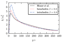
|
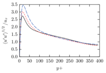
|
| (a) Turbulence kinetic energy. | (b) Stream-wise velocity fluctuations . |
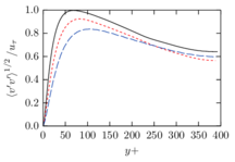
|
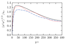
|
| (c) Wall-normal velocity fluctuations . | (d) Cross-stream velocity fluctuations . |
| Figure 22: Channel flow – turbulence kinetic energy and Reynolds stresses obtained using , compared to Moser et al. [51]. | |
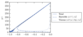
|
| Figure 23: Channel flow – average stress profile obtained using hexahedra and fixed . |
We observe that the results obtained with linear hexahedra are closer to the expected values than those obtained with linear tetrahedra in all cases. This was to be expected, as hexahedra use trilinear shape functions, which define a richer interpolation than the linear functions used in tetrahedra.
In light of the fact that the formulation we are using has a free parameter, , which is set a priori, we are interested in studying how the solution is dependent of its value. To investigate this, we simulated the problem with the same settings, changing only the value of . The results obtained using a tetrahedral mesh with divisions along each coordinate direction are shown in Fig. 24, where the statistics obtained with and a tetrahedral mesh in the previous test, corresponding to the dashed curve in Fig. 21 and Fig. 22 are compared to those obtained with the same mesh and different values of . It is observed that there is not a large amount of variation between the different cases, although the case tends to display a lower level of velocity fluctuations in all directions. This suggests that small values of , which give more weight to the gradient diffusion term, result in a solution that is more diffusive overall.
3.6.3 Variable combination parameter
The next set of tests was performed using Eq. 3.212 to assign a value to the combination parameter , while keeping the remaining simulation settings as in the fixed beta case. The minimum value of the coefficient was set to for the first tests, which produced the average velocity distribution presented in Fig. 25 and the velocity variances shown in Fig. 26, where we compare them to to the results obtained for a fixed coefficient in previous simulations.
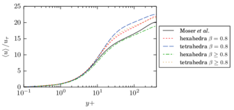
|
| Figure 25: Channel flow – average stream-wise velocity profiles using a fixed or dynamic combination parameter. |
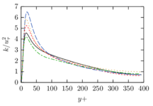
|
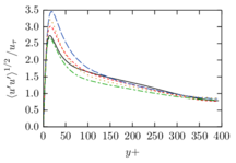
|
| (a) Turbulence kinetic energy. | (b) Stream-wise velocity fluctuations . |
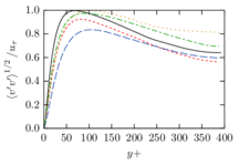
|
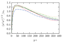
|
| (c) Wall-normal velocity fluctuations . | (d) Cross-stream velocity fluctuations . |
| Figure 26: Channel flow – turbulence kinetic energy and Reynolds stresses using a fixed or dynamic combination parameter. See legend in Fig. 25. | |
We can see in the figures that the average velocity profiles are generally lower to those obtained in the fixed cases and closer to those obtained from DNS data. Conversely, the velocity fluctuations measured in the stream-wise direction are somewhat lower than in the fixed simulations, resulting in a turbulence kinetic energy that is much closer to that obtained from DNS simulations.
As in the previous case, we are also interested in quantifying the impact that the choice of a limit value for the combination coefficient has in the obtained solution. To test its influence, we ran several simulations for tetrahedra (Fig. 27) and hexahedra (Fig. 28), changing the limit value for . We consider that the results show minor variations depending on the choice of parameter, at least for large values of .
We also studied the sensitivity of the solution to the choice of mesh size. The results obtained using a coarser mesh of hexhahedra or tetrahedra are compared in Fig. 29 to those obtained with the meshes used in the previous examples. As before, there is a clear difference in the behaviour of tetrahedra and hexahedra. In particular, it seems that the coarser tetrahedral mesh is insufficient to reproduce the features of the problem, resulting in a significantly larger average velocity.
As a final validation, we compared our results to those obtained using a GLS formulation on the same finite element mesh. The results of this test are shown in Fig. 30.
3.6.4 Summary of the results
To conclude the analysis of the turbulent channel flow at test case we summarize the main results. A first general observation is that hexahedra produce much more accurate solutions than tetrahedra for a given mesh size. A difference in accuracy was expected, as the interpolation obtained using hexahedra is richer, but we have found it to be large in our mesh studies. An observation of Fig. 29 suggests that tetrahedra are required to obtain results comparable to hexahedra, which represents 48 times more elements in total. In spite of this, we will continue to use tetrahedra in the following examples, due to their flexibility in meshing complex geometries.
As the formulation we are proposing has a free parameter, the combination parameter , we wanted to study the sensitivity to its value. In the cases where the parameter was fixed throughout the simulation, the general trend is to obtain lower variances the smaller the coefficient, which corresponds to giving more weight to the gradient diffusion term (see Fig. 24). This suggests that the gradient diffusion term introduces a significant amount of numerical dissipation, producing more homogeneous solutions. However, it must be noted that the average velocity profile is much less sensitive to the choice of parameter, producing very similar results in all cases.
If the combination parameter is set on each element according to the local weighting function of Eq. 3.212, the obtained velocity profiles are generally lower than those obtained with a fixed parameter and measured variances show a better agreement with the DNS data, specially in the correlation, which is the larger contribution to the total turbulence kinetic energy (see Fig. 26). In this case, the only external parameter is the minimum admissible value of , but our experiments show that the results are not very sensitive to this parameter, at least if it is large enough, as can be observed in Fig. 27 for tetrahedra and Fig. 28 for hexahedra.
Finally, we compared our approach to using a standard GLS stabilization, which, for linear elements, is equivalent to the Q-ASGS formulation presented in Chapter 2. The results, shown in Fig. 30, suggest that the formulation we propose results in a closer approximation to DNS data than the reference for a given mesh size. We propose two reasons a justification for this result. On one hand, we introduce a new term, the gradient diffusion, which has been shown to introduce an additional source of dissipation. On the other, the formulation we propose, unlike GLS, does not include a div-div term, which was shown in [27] and in our own results in the previous chapter to have a negative impact in the turbulent channel case.
Based on the results obtained in this set of tests, we conclude that setting the combination parameter locally, limited to a minimum value of , is the variant that better approximates the reference solution. As a result, we will adopt this formulation for the remaining cases.
3.7 Flow around a cylinder
The flow over a circular cylinder is a classical problem in CFD simulations, which has been studied extensively, both experimentally and numerically, as can be verified for example in the review of [63]. Flow over circular cylinders exhibits a variable behavior depending on the Reynolds number, due to the different vortex shedding mechanisms that develop on the wake [64]. As a benchmark example for the FIC formulation, we studied the case corresponding to a Reynolds number based on the diameter of the cylinder and the inflow velocity. This case was studied experimentally in [65] and numerically in [66] or [67]. In this section, we will use a numerical set up similar to that of [66] and compare our results to those presented in that reference.
We simulated the flow over a cylinder with dimensionless diameter using a domain of , centered on the cylinder, in the plane normal to the cylinder's axis, and in the span-wise direction. The simulation is run for dimensionless time units (made dimensionless using the inflow velocity and the diameter ) with a dimensionless time step , which should provide sufficient resolution to capture the main vortex shedding frequency.
The domain for the problem is presented in Figure 31. Consider the axes , and , aligned in the stream-wise, cross-stream and span-wise directions respectively, and let , and , be the components of the flow velocity in each of the three coordinate directions. We are interested in measuring the velocity history in selected planes in the wake of the cylinder, chosen to coincide with those reported in the reference.
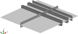
|
| Figure 31: Flow around a cylinder – simulation domain and measurement planes. |
Linear tetrahedral elements have been used to mesh the domain, with sizes ranging between near the cylinder to in the far regions. This resulted in a total of million nodes and million elements. The velocity is fixed to a constant for the inlet and to zero on the cylinder surface. Periodic boundary conditions have been used in the span-wise direction, while a no-penetration condition has been imposed in the far sides on the cross-stream direction. The combination parameter for the FIC formulation is set locally for each element using the dynamic formulation, with a limit value of .
The instantaneous stream-wise velocity field on the central – plane at the end of the simulation is shown in Fig. 32. The velocities on the – plane for the same time instant are shown in Fig. 33. From the stream-wise velocity component in Fig 33a, the formation of a recirculation zone just after the cylinder can be observed. Similarly, in Fig. 33b, which shows the instantaneous cross-stream component of velocity , the alternating direction of the velocity suggests the formation of a vortex trail.
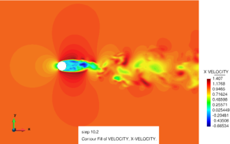
|
| Figure 32: Flow around a cylinder – instantaneous stream-wise velocity on the – midplane. |

|

|
| (a) Stream-wise velocity . | (b) Cross-stream velocity . |

| |
| (c) Span-wise velocity . | |
| Figure 33: Flow around a cylinder – instantaneous velocities on the – midplane. | |
While the instantaneous velocity distributions give us a qualitative idea of the flow, we are interested in studying the statistics of the cylinder wake, which can give us a more quantitative idea of the quality of the simulation. We computed the average velocity in the stream-wise and cross-stream directions on different – sections (that is, normal to the mean flow) on the wake of the cylinder. The results in terms of averages, compared to those of [66], are shown in Fig. 34 for the near wake and in Fig. 35 for the far wake.
Observing the results, we can see that we obtain a close agreement with the reference, although the formation of the wake is slightly delayed when compared to the reference. This can be seen by considering that the average velocity defect on the wake should start as a deep U-shaped trough just behind the cylinder, where the average flow in the recirculation zone is very small or negative on average, and become wider and shallower (closer to the inflow velocity ) as the wake develops. In general, our profiles are below the expected curve.
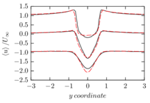
|
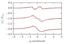
|
| (a) Stream-wise velocity . | (b) Cross-stream velocity . |
Figure 34: Flow around a cylinder -- average velocities in the near wake. Reference  , present work , present work  . From top to bottom: , , . . From top to bottom: , , .
| |
In addition, we have also computed the variance of the stream-wise velocity , shown in Fig. 36a for the near wake and Fig. fig:fic_cyl_corr_far_uu for the far wake. The obtained variance is smaller in general than expected, which suggests a smoother flow and a more diffusive solution. The cross-correlation is shown in Fig. 36 on the same planes where it was reported in the reference. This result shows some irregularity, in our solution as well as in the reference, which might be reduced with a longer simulation time.
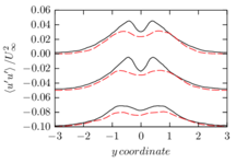
|
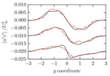
|
| (a) correlation. | (b) correlation. |
Figure 36: Flow around a cylinder -- velocity correlations in the far wake. Reference  , present work , present work  . From top to bottom: , , . . From top to bottom: , , .
| |
Finally, we have computed the drag coefficient and the Strouhal number , which represents the dimensionless vortex shedding frequency, as given
|
|
(3.266) |
where is the average force applied by the fluid on the surface of the cylinder in the stream-wise direction and is the vortex-shedding frequency on the cylinder tail, which we have calculated from the lift force history . The results, compared to those reported in [66], are reported in Table 2.
| Analysis | ||
| Present simulation | ||
| Numerical [66] | ||
| Experimental (reported in [66]) |
The results obtained for this case show in general good agreement to reference values in terms of the average solution. Variances, while in qualitative agreement with the expected results in terms of spatial distribution, tend to be underestimated. This suggests that the obtained solution has larger dissipation than required, smoothing out peaks in the fluctuating solution. It would be interesting to repeat the same simulation with hexahedra or with a finer tetrahedral grid, to see which fraction of this dissipation is due to mesh resolution or to the formulation itself.
3.8 Flow around a solar collector
As a final example we wanted to test the capabilities of the formulation when applied to an industrial problem. For this, we simulated the wind flow around a parabolic trough solar collector and compared it to experimental data. A parabolic trough is an array of parabolic mirrors that concentrate solar rays in their focus, where the solar energy is collected and used to operate a steam turbine generator. The mirrors can be large structures (the one we are studying is a parabola with a 5 meter aperture) and are susceptible to damage due to strong winds. As such, there is interest in studying the wind load over the mirror, both numerically and experimentally.
We are using one of such experiments as a reference, where a 1:25 scale model of a single mirror was placed in a wind tunnel. This experiment was performed for Abengoa Research, which has given us access to the data, and was reported in [68,69]. Note that, as requested by the company, we are providing all our results in scaled form to protect intellectual property.
Due to the larger scale of the model compared to the previous examples, we will not attempt to reproduce the full boundary layer and the Werner-Wengle wall model [70] will be used to introduce the equivalent wall friction close to solid surfaces. Additionally, as we are trying to reproduce a wind tunnel experiment with a turbulent incoming flow, we need to generate a time-dependent inlet condition which bears a statistical resemblance to a real wind signal (see for example [71] or [72]).
The geometry of the collector is shown in Fig. 37 at full scale. To reproduce the different configurations of the collector as it rotates over its axis to follow the sun, the seven cases shown in Fig. 38 modifying the pitch of the mirror in increments of . The average wind is always assumed to reach the collector frontally, so that the mirror presents the maximum possible area to the flow.
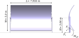
|
| Figure 37: Parabolic collector dimensions (full scale). |

|

|

|

|

|

|
| (a) | (b) | (c) | (d) | (e) | (f) |

|
|||||
| (g) | (h) | ||||
| Figure 38: Solar collector – pitch angles considered in the simulation. Wind blows from the left. | |||||
We simulated the collector at model scale (1:25), reproducing the wind tunnel experiment. The collector was placed on a fluid domain of at model scale in the stream-wise, cross-stream and vertical directions, respectively, at from the inlet.
The incoming wind is generated using the model of [71] to follow a Kaimal wind spectrum [73] with a reference stream-wise velocity at (corresponding to at full scale) and a wall roughness ( at full scale). The air is assumed to have density and viscosity , resulting on a Reynolds number calculated using and .
The calculation was performed with an unstructured tetrahedral mesh, with mesh sizes ranging from close to the mirror surface to on the far regions. This resulted in approximately nodes and elements for each simulation.
Instantaneous distributions of velocities and pressures close to the collector are shown in Fig. 39 for the case with pitch angle and in Fig. 40 for the case of as an example of the results. As can be seen in the figures, a vortex trail develops due to the presence of the collector.
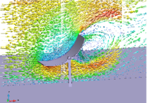
|
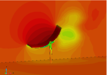
|
| (a) Velocity vectors. | (b) Pressure contours. |
| Figure 39: Solar collector – instantaneous velocity and pressure fields for pitch angle . | |
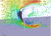
|
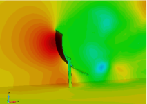
|
| (a) Velocity vectors. | (b) Pressure contours. |
| Figure 40: Solar collector – instantaneous velocity and pressure fields for pitch angle . | |
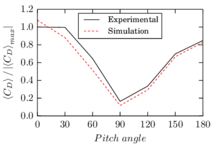
|
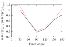
|
| (a) Average drag | (b) RMS drag |
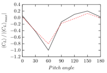
|
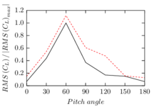
|
| (c) Average lift | (d) RMS lift |
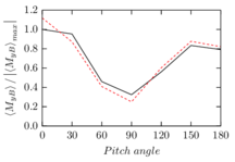
|
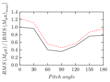
|
| (e) Average moment | (f) RMS moment |
| Figure 41: Solar collector – average reactions. | |
The simulation is performed for a sufficiently long time for the flow to become statistically steady and obtain a data set on this regime so that meaningful statistics can be obtained. The forces on the mirror are integrated at each time step and recorded over time. These results are used to compute the drag and lift coefficients and the moment , calculated around an axis placed on the base of the structure, as shown in Fig. 37. The reactions are made dimensionless using and the collector dimensions , as follows
|
|
(3.267) |
the resulting statistics for the different pitch angles considered are compared to the experiment in Fig. 41. The results are presented relative to the maximum value in each experimental curve as requested by Abengoa.
As was the general trend in the previous example, we achieve good accuracy in terms of the averages, while the results in terms of fluctuations (the RMS in this case) tend to be less accurate. In any case, we consider that this case serves as a proof of concept, showing that the formulation has potential to solve problems of practical interest in engineering, with complex geometries and variable inlet conditions.
3.9 Summary and conclusions
In the present chapter we have introduced a new FIC-based formulation for incompressible flows. The main features of our method are the presence of a new term on the momentum equation, which introduces an additional non-isotropic dissipation in the direction of the velocity gradients, and a stabilized formulation for the mass equation which is based on a second order FIC balance in space and represents an incompressible Eulerian version of the method presented for quasi-incompressible flows in [59].
This method has a free parameter in the combination coefficient that defines the relative weights of the classical streamline diffusion and the new gradient diffusion term in the stabilization of the momentum equation. We have proposed a way to define this coefficient dynamically, with the intent of improving the results and reducing the dependence of the solution on the free parameter.
We have tested the method with several application examples. The first example presented is the turbulent channel flow at , where we have tested the different variants of the method. The main conclusions we extracted from the simulations can be summarized as follows:
- Hexahedral meshes provide significantly better results than tetrahedra, with hexahedra producing results of comparable quality to tetrahedra.
- The method is not very sensible to the free parameter , at least for values of , for either the fixed or dynamic variants.
- Using the dynamic formula for the coefficient results in a better approximation to the DNS curves, although the problem to be solved becomes more non-linear.
Finally, the method was then applied to large turbulent flow simulations, first the flow around a cylinder and then an industrial-scale simulation of the wind flow over a parabolic solar collector. In this last case, due to the larger Reynolds number, the method was used in combination with the Werner-Wengle wall model to introduce the right dissipation on the walls without reproducing the full boundary layer.
The results show that the presented method is capable of reproducing the features of the flow and shows promise in the application of the method real world examples of industrial interest.
4 Parallel implementation
4.1 Introduction
We have already remarked that one of the reasons why turbulent flow problems are challenging is that they involve fluid motions with very different characteristic sizes and, as a result, their numerical simulation requires very fine discretizations, both in space and in time. Even with the introduction of turbulence modeling, LES simulations for problems of practical interest in engineering require significant computational resources and are well beyond the range of what currently can be calculated in a reasonable time with a desktop computer.
Currently, the overwhelming majority of High Performance Computing (HPC) machines are distributed memory clusters (see for example the TOP500 list of the most powerful computer systems [74]), in which many individual processors work in parallel on different parts of the problem to be solved. Such machines are organized as groups of interconnected calculation nodes, where each node contains one or several processors and a block of memory. In this calculation framework, there exists a very clear distinction between local data, stored in the node's memory, which is readily available to the processor, and non-local data, stored in a different node, which has to be requested to that node requires many more computation cycles to access.
In the context of finite element simulations, large problems can be solved using a distributed memory approach by dividing the model domain into parallel subdomains, each containing a fraction of the finite element mesh, and assigning each of them to an individual processor. This requires careful design of the calculation software to solve the global problem while minimizing the exchange of information between the individual subdomains.
In this sense, a part of the programming work presented here represents a contribution to an ongoing work in our research group to improve the performance of Kratos Multiphysics in distributed HPC clusters. This chapter will be devoted to presenting some of the adaptations required for distributed memory simulations and to test the parallel performance of the resulting implementation.
We will focus our presentation on some aspects of parallelization that have required the most attention to achieve the goals of the present work. The first of these is the division of the original finite element mesh into parallel subdomains and the generation of a communication strategy to efficiently exchange information between them. To present this, we briefly describe in Section 4.2 how distributed data is organized in the code and how it can be shared among processes, while Section 4.3 deals with the generation of this distributed data from the complete problem.
The second aspect that will be considered is the parallel efficiency of the complete solver. We describe some details of the assembly and solution of the problem's linear system that require attention in a distributed memory context in Section 4.4 and evaluate the parallel performance of the complete solver in Section 4.5.
Finally, as we have seen in Chapters 2 and 3, in turbulent flow analysis the quantities of interest are frequently statistical results, obtained from spatial and/or temporal averaging. In the context of large data sets and HPC, the efficient calculation of statistical results requires careful consideration. This will be discussed in Section 4.6, where the approach we have followed will be described.
Some final thoughts and future lines of improvement are presented in Section 4.7.
4.2 Distributed memory model
While there are multiple strategies to distribute data for finite element problems, the approach of Kratos Multiphysics consists in dividing the mesh into discrete subdomains, such that each individual element is assigned to a given processor, as shown for an example problem in Fig. fig:pi_partition_elements. In this approach, some of the mesh nodes will appear in two or more different subdomains, as they belong to elements assigned to different partitions. Such nodes will be called interface nodes.

|

|
| (a) Element partition. | (b) Node partition. |
| Figure 42: Division into subdomains. | |
It is critical to the solution of the problem that nodal data for interface nodes is consistent across the different partitions, which requires its synchronization given points of the solution procedure. To simplify this exchange of information, we found it convenient to also assign nodes to a given partition, which holds the reference values for nodal data. From the point of view of a calculation process, nodes which belong to its partition are defined as local nodes, while interface nodes which are known but are assigned to a different partition are called ghost nodes. An example of such partition is shown in Fig. fig:pi_partition_nodes, where local nodes are represented with a full circle in the color of the partition and ghost nodes are represented with empty circles. In the same figure, dashed lines represent inter-process communications which will be required during the solution procedure.
In a communication strategy, it is important to define not only which partitions have to share information with each other but also the order in which such communication is done. For example, the communication graph for the partition of Fig. 42 is shown in Fig. fig:pi_communication_all.

|
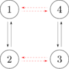
|
| (a) All links. | (b) Optimal. |
| Figure 43: Communication patterns for the partition of Fig. 42. | |
The simplest approach would be transferring data in order, starting from one of the pairs and exchanging data one by one. This approach would have poor parallel performance as, while a given pair of processes exchanges information, the others are idle. Furthermore, the total number of exchanges required grows rapidly as the number of processes is increased, resulting in a significant fraction of the total calculation time spent waiting for communication.
A more efficient approach is to try to group communications in a way that processes are never idle, such as in Fig. fig:pi_communication_good, considering one first stage where process 1 communicates with 2 and 3 with 4, followed by a second phase where process 1 communicates with 4 and 2 with 3. Reducing the number of total communication stages and, in this case, keeping all processes busy at all times.
In the case of Kratos Multiphysics, an existing code which had to be adapted for parallel simulations, the existing data structure had to be adapted to work in a distributed memory context. While we won't go into the details of the Kratos structure here (the interested reader is directed to [75,28]), we will just say that all model data is stored in an entity known as ModelPart, which contains the definition of the mesh and the associated nodal or elemental data. In a parallel context, each process defines its own ModelPart, which in this case contains all elements in the subdomain assigned to that process and all nodes (both local and ghost) required to perform the simulation.
Data transfer across processes was achieved by adding an additional component in the ModelPart, the Communicator, which handles parallel communication [29]. This object stores the communication strategy (which process will I communicate with on each stage) and the lists of local and ghost nodes to be exchanged in each stage. When data transfer is required, the Communicator collects the nodal data to send on each stage and exchanges it with the corresponding process using Message Passing Interface (MPI) calls [76].
One of the advantages of this approach is that it allows to reuse a very significant part of the code between serial and parallel simulations. To do so, the code is programmed with the parallel implementation in mind, with all required data transfer performed through Communicator functions. Then, two different Communicator classes are implemented, one for parallel executions that works as defined above, and another for serial runs, which does nothing. With this approach, we have been able to significantly reduce code duplication, minimizing the maintenance problems related to keeping up to date a serial and a parallel version of the same code.
4.3 Partitioning of input data
Once we have a data structure that can be used to hold and communicate distributed finite element data we need to be able to, given a simulation domain, generate a partition in as many subdomains as parallel processes will be used in the simulation and a communication strategy to transfer data between them. In Kratos Multiphysics, the usual situation is to have a single input file containing the entire simulation mesh, typically generated with GiD [77]. The partitioning procedure in this case constitutes one last step of the pre-process of the problem, generating separate inputs for each simulation domain.
The partitioning process should generate balanced partitions, that is, all partitions should contain a similar number of elements and nodes, to ensure that the computational load is homogeneous for the different processors. A poorly balanced partition means that the processes with lighter work loads have to wait for the other to finish, resulting in longer total calculation times. In addition, the partition should minimize the amount of communication required relative to the total calculation time. This is sometimes expressed by saying that the computational cost of the simulation is proportional to the number of elements, that is to say, to the volume of the partition, while the communication costs are proportional to its surface. Therefore, a good partitioning algorithm should minimize the surface to volume ratio for the partition.
We use a the capabilities provided by the METIS library [78], which generates a partition using a multi-level approach. Starting from a graph of nodal connectivities, multi-level methods are based in generating progressively coarser graphs by grouping close nodes together and generating an optimal partition of the coarsest graph. The partition is then refined by undoing the coarsening. Such approaches are considered to provide good quality partitions for unstructured meshes.
As mentioned, the approach of METIS is based on the nodal graph, and provides a partition of the nodes. While there are some capabilities in METIS to divide the elements, they work for homogeneous meshes, composed of a single type of element1. This was insufficient for our needs as, due to the way boundary integrals are implemented in Kratos Multiphysics, the meshes in the problems we are simulating are typically heterogeneous. A simulation, for example, may include tetrahedral volume elements, triangular faces used to apply Neumann boundary terms or wall laws, for example, and point-to-point links to apply periodic boundary conditions. All of these have to be taken into account when building the nodal graph and the latter in particular has a significant impact in the final partition, as it typically indicates a relation between two nodes that are geometrically far away.
Element partitioning is achieved by following some simple rules. First, if all nodes in the element belong to the same partition, the element is automatically assigned to that partition. If its nodes are assigned to different partitions, then the element is preferentially assigned to the partition that owns most of the nodes, but keeping into account load balance: if that partition already contains more elements than the others, the element will be assigned to one of the partitions that own the remaining nodes.
Once this initial distribution in done, partitions are checked again for isolated nodes. Due to the way the element distribution procedure works, it can happen that some domain has a node but no elements that contain it. This situation would generate unnecessary communication, as the partition would have to store and update the reference data for a node it never uses, so those nodes are reassigned to a partition that needs them.
With the partition complete, the next step is to generate a communication strategy. To achieve this, we start by building the domain graph, stored as a matrix where term is non-zero if there is an interface between partitions and . For example, the graph for the domain of Fig. 42 is
|
|
(4.268) |
The strategy to organize the communications is known as coloring, as the problem is equivalent to assigning a color to all edges in the graph such that no two edges of the same color reach the same node. Once this is done, communication is achieved by transferring data across all interfaces of the same color at the same time. To perform the coloring, we use a simple approach, always assigning the first available color as they are needed, presented as Algorithm 3. This has been shown to be sub-optimal, as in the worst case it can use up to twice as many colors as the number of partitions. However, in our experience, obtained solutions are not usually as bad. A more concerning issue is that it is significantly more computationally expensive than an approach such as [79], which would produce optimal strategies.
|
|
Algorithm. 3 A simple coloring procedure. |
For the partition of Fig. 42, this procedure results in the following color matrix, where each column corresponds to a color and unused columns have been omitted:
|
|
(4.269) |
If we take each row of as a parallel process and each column as a stage in the communication procedure, indicates which partition we have to communicate with at a given step. In this case, we recover the communication pattern of Fig. fig:pi_communication_good. Note that, for more complex cases, we may obtain a communication pattern where some processors are idle for some of the communication steps. If this happens, the corresponding positions in contain a .
The final step in the procedure is to write each partition and the associated communication data (local and ghost nodes and the communication strategy) to separate input files, one for each simulation process. Once this is done, the parallel solution procedure can start.
Taking into account all steps, the partition procedure can summarized as:
- Read nodal connectivities and call METIS to partition the node graph.
- Distribute elements.
- Check each partition for isolated nodes, and move these to other partitions.
- Use a coloring procedure to generate a communication strategy.
- Write partition data to separate input files, one for each parallel process.
(1) More recent versions of METIS do provide the possibility of partitioning heterogeneous meshes, but at the time of implementation we were limited by the relatively old versions available in the clusters we had access to.
4.4 Distributed solution
Once the problem domain is partitioned and a communication strategy has been determined the model is prepared for a parallel simulation. Compared to a serial solution, a distributed memory simulation introduces additional complications in the procedure. First, as the finite element mesh was divided into subdomains, the system matrix will also be distributed, with the contribution from each individual element being computed in the process that holds it. More importantly, once the system matrix has been assembled, it has to be solved using a distributed algorithm which can take full advantage of the parallel environment. In fact, the choice of a scalable parallel solver has a crucial impact on the parallel performance of the code. Finally, once the problem has been solved, the updated values for the variables are synchronized to ensure that nodal variables are consistent across the processors.
In terms of the parallel finite element assembly procedure, Kratos Multiphysics relies on the Trilinos library [80] to construct and manage the system of linear equations that has to be solved on each iteration. In particular, Trilinos' Epetra package provides an implementation of distributed memory sparse matrices and vectors that can be used to hold the system data and communicate it to other processes when needed.
Finite element matrices can typically be stored in a sparse format, since most of the terms in the system matrix are zero. Therefore, just as in the serial case, before constructing the system matrix and vector we need to determine the sparsity pattern and allocate the required memory. This is done based on the nodal graph: given that each matrix row (and column) corresponds to a given degree of freedom in the problem, an entry will be non-zero only if an element exists in the mesh connecting the nodes that the row and column degrees of freedom are associated to. Since the matrix implementation in Kratos Multiphysics is row-based, each row is considered local to the processor that owns the node associated to that row's degree of freedom. With this information we can generate the data structure that will hold the system data, which is ultimately an instance of Trilinos' Epetra_FECrsMatrix for the system matrix and an Epetra_FEVector for the right hand side vector.
The construction of the sparse data structure is a relatively time-consuming operation, but can be done once the first time the matrices have to be constructed and reused in subsequent iterations, as long as the mesh connectivity pattern is preserved. Note that this is true for the examples in the present chapter, as well as those in Chapters 2 and 3, but will not be the case for the adaptive mesh refinement simulations of Chapter 5.
Once the data structure is ready, we iterate over all elements in the model, calculating the elemental contribution to the problem and assembling it into the system matrix and vector. However, since each row receives contributions from all elements that contain the associated node, parallel communication is required to account for contributions coming from elements associated to a different processor. To minimize the amount of parallel communication required, the global matrix is assembled locally at first to add the contributions from all local elements. Once this is done, rows that receive contributions from multiple subdomains are assembled by adding the contributions from each and communicating the result to other partitions.
Once the system is solved, we encounter the inverse problem: the new nodal values have to be communicated from the process that stores that particular row to all processes that have a copy of the corresponding node. Again, this requires a communication step.
The (efficient and scalable) parallel solution of the system is, by itself, a different and very challenging problem, which will only be briefly presented here. Given the size of the systems to be solved, direct methods are not applicable due to their memory requirements and computational cost. A more adequate choice is to use parallel implementations of Krylov methods [81], which are very efficient solvers but are not designed as parallel algorithms and tend to require an increasing number of iterations to converge as more partitions are introduced. Alternatively, a variety of algorithms designed for parallelism exist, including Algebraic Multigrid (AMG) algorithms [82,83], which introduce a hierarchy of increasingly coarser versions of the original problem and use the coarser solutions to accelerate the convergence of the finer problem, solution strategies based on domain decomposition techniques, in which each domain is solved separately and its effect on its neighbors is felt through boundary terms and deflation techniques, which combine an aggressive coarsening with domain decomposition.
In Kratos Multiphysics, the usual approach has been to rely on the linear solvers provided by the Trilinos library, which includes both Krylov solvers on its Aztec package [84] and Multilevel algorithms through the ML [85] library. This approach was used for example to simulate the benchmarks presented in [29]. In the following pages we will use a different linear solver in combination with the incompressible flow formulation presented in Chapter 2. This solver is provided by the AMGCL library [86,87], currently under development, and is based on combining a deflated approach where the coarse problem is given by the MPI partition with an AMG solver within each subdomain.
4.5 Benchmark cases
To evaluate the performance of the parallel implementation of our solver we have performed some simulations of large test cases. Note that, unlike in the remainder of this work, here we are more interested in the performance of the algorithm than in the quality of the solution. Therefore, we simulate very short time spans, mainly to sample the computational costs associated to the procedure, and the resulting solutions can not be considered as an accurate representation of the real flow. These examples were simulated in the Gottfried cluster of the North-German Supercomputing Alliance (HLRN).
4.5.1 Flow around an inflatable structure
The first test case is adapted from a real simulation mesh courtesy of the uLites1 project team. This project was concerned with the design and construction of inflatable structures subjected to wind loads and included the comparison of numerical and wind tunnel experiments on the designed structure. Here we take one of the simulation meshes, representing the geometry of a rigid scale model that was used in wind tunnel tests and simulate the flow around it using the Q-ASGS formulation described in Chapter 2.
The model, presented in Figure 44, is composed of four cylindrical tubes with a diameter of folded into a semicircle with a radius of , measured from the tube centerline. The simulation domain, shown in Figure 45, measures in the streamwise, cross-stream and vertical directions, respectively, and the inlet is placed at of the axis of the module.
The incoming flow is modeled as air with density and viscosity flowing at , which corresponds to a Reynolds number of approximately relative to the radius of the module. Velocity is fixed to zero on the floor and the surface of the module, while a no-penetration condition is used on the sides of the calculation domain. Note that, given the mesh resolution, a wall law would be a more adequate boundary condition for the solid boundaries, but we will not use it here in order to concentrate our attention on the fluid solver.

|

|
| (a) Top view. | (b) Side view. |
| Figure 44: Inflatable structure model – geometry of the module. | |
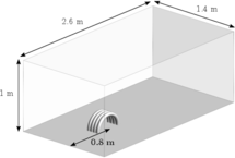
|
| Figure 45: Inflatable structure model – dimensions of the simulation domain. |
We define two different simulation meshes. The first is an unstructured tetrahedral composed of around nodes and million elements, with sizes ranging from close to the surface of the module to in the far regions. The second is obtained by the bisection of the element edges of the first, obtaining 8 elements from each original tetrahedron, and contains a total of million nodes and million tetrahedra. The flow is simulated for five time steps, using a step size for the element mesh and for the million element case, halved to maintain the same Courant-Friedrichs-Lewy (CFL) number.
The time required to perform different parts of the procedure for the coarser mesh is summarized in Table 3. The solution of five complete time steps required a total of between and system solutions, which took between and seconds of wall clock time when going from to parallel processes. We notice that the simulation time is dominated by the solve phase, which is more expensive than the finite element assembly in all cases.
| MPI processes | |||||
| Assembly time | |||||
| Solution time | |||||
| Num. of iterations | |||||
| Assembly time | |||||
| Assembly speedup | |||||
| Solution time | |||||
| Solution speedup | |||||
| Assembly time | |||||
| Assembly speedup | |||||
| Solution time | |||||
| Solution speedup | |||||
| Solution time | |||||
| Num of iterations | |||||
| Average solution | |||||
| Solution speedup | |||||
| Global speedup | |||||
We also observe that the first iteration of the finite element assembly procedure takes more time than subsequent iterations, since it includes the calculation of the sparsity pattern for the system matrix and the allocation of the required memory. We notice that, far from showing parallel scalability, the time spent in the first iteration is in fact increased as more processors are used. We consider this to be consistent with the fact that the set-up phase requires abundant parallel communication to determine the shape and ownership of each matrix row, which takes more time as more processes are involved. In any case, we have not considered the time of the first iteration in calculating averages, since it involves more operations than the rest.
Finally, we remark that we have considered the last time step separately from the rest. The cause for this is that, for some of the cases, the first few system solutions stop due to the solver reaching the maximum allowed iterations instead of fulfilling the convergence requirements. This is due to the initial condition being a bad first guess of an equilibrium solution, which means that in the first few iterations the system is harder to solve and the algorithm fails to achieve the desired error tolerance.
We feel that comparing converged and non-converged iterations skews the scalability results, since we want to measure the time required to achieve a solution of a given quality, not the time it takes to perform an arbitrary number of iterations. For this reason we measured the time required to solve the last time step, where all system solutions converged in all cases, and present it separately for the different cases. Likewise, the values given as global speedup in the results have been computed considering one average system assembly plus the average time taken in solving a single linear system on the last time step.
The times measured for the finer test case, using a million element mesh, are presented in Table 4. The behavior of the method is qualitatively the same, and the same remarks about the additional cost of the first iteration are applicable.
| MPI processes | ||||||
| Assembly time | ||||||
| Solution time | ||||||
| Num. of iterations | ||||||
| Assembly time | ||||||
| Assembly speedup | ||||||
| Solution time | ||||||
| Solution speedup | ||||||
| Assembly time | ||||||
| Assembly speedup | ||||||
| Solution time | ||||||
| Solution speedup | ||||||
| Solution time | ||||||
| Num of iterations | ||||||
| Avg. solution | ||||||
| Solution speedup | ||||||
| Global speedup | ||||||
The time costs of a single solution iteration are represented graphically in Fig. 46, where the first iteration is compared to a typical iteration, calculated using the average time for the build phase and the last time step average for the solve phase. Here again we see a different behavior for the first and a typical iteration, due to the cost of determining the structure of the system matrix and allocating the required memory. Once this is done, in subsequent iterations the computational cost is driven by the system solution, which takes considerably more time in all cases.
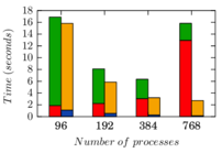
|
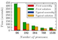
|
| (a) 4 million element mesh. | (b) 35 million element mesh. |
| Figure 46: Inflatable structure test – time costs of a single iteration. | |
To measure the parallel performance of the procedure we have measured the strong scalability of the algorithm, that is, we have compared the required taken to solve the same problem with an increasing number of processors. This is presented graphically in Fig. 47 for the million element case. We can observe that the scalability behavior is basically driven by the system solution, which dominates the solution cost. The parallel efficiency of the finite element assembly is close to linear, taking times less time when using eight times more processors, although parallel performance degrades when the number of elements per processor is low. This is to be expected, since the communication cost increases when using more processors while the individual work loads decrease as the number of elements per processor is reduced, which means that the total cost for large enough numbers of processors is dictated by communication operations.
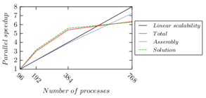
|
| Figure 47: Inflatable structure test – parallel speedup for the million elements. |
The behavior of the solution phase is possibly more unexpected. The costs reported in Table 3 correspond to a better than linear scaling, which is a consequence of the design of the AMGCL solver, which requires less iterations for larger numbers of processors. In any case, we observe that parallel performance is good for smaller numbers of processors but stops being worthwhile for the last test, since doubling the number of processors from to only produces a modest reduction in calculation costs. Again, this is consistent with communication dominating the total cost of the procedure.
The same strong scalability study can be done for the million elements grid, producing the results presented in Fig. 48, and yields results that are qualitatively similar to those obtained for the million element case. Here, however, the larger problem size means that we can use more processes before communication costs dominate, obtaining better scalability results for a given number of processors.
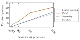
|
| Figure 48: Inflatable structure test – parallel speedup for the million elements. |
Finally, we can use the results we have to estimate the weak scalability of the algorithm. Weak scalability is calculated by comparing the cost of solving a problem with a given number of processors to that of solving a larger problem with a proportionally larger number of processors. In our case, the cost of assembly is proportional to the number of elements while the cost of the system solution is proportional of the number of degrees of freedom and therefore to the number of nodes. Refining the problem, we obtained a mesh that contains exactly times more elements while multiplying the number of nodes by approximately . We used this fact to estimate the weak scalability by comparing the time used to solve the million element problem with the time required to perform the same operation using 8 times more processors in the million element mesh. This is presented in Table 5, where we can see that, while the build phase does scale weakly, the fine problem takes up to four times as long to solve for the fine mesh.
| Time ratio (fine problem/coarse problem) | ||
| Average assembly time ratio | ||
| Typical solution time ratio |
(1) Ultra-lightweight structures with integrated photovoltaic solar cells: design, analysis, testing and application to an emergency shelter prototype. EC project within the Seventh Framework Programme, Grant No. 314891.
4.5.2 Flow around a race car
The second example we used to benchmark the solver is the flow around a race car, using the geometry shown in Fig. 49, adapted from [88]. The car is long, wide and high and it is placed within a fluid domain measuring in the streamwise, cross-stream and vertical directions respectively. The problem being simulated consists in a flow of air (, ) at , which corresponds to a Reynolds number of .
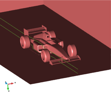
|
| Figure 49: Race car test – geometrical model. |
As in the previous case, the mesh is not designed for high-quality simulation (this would require a boundary layer mesh or at least a wall law) but to test the parallel capabilities of the solver. We test two different meshes: the first one contains million nodes and million tetrahedral elements with sizes ranging between close to the surface of the car and in the far regions, while the second one is obtained by the edge refinement of the first, which is composed of million nodes and million elements. Some details of the finest mesh used in the tests can be observed in Fig. 50.
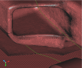
|
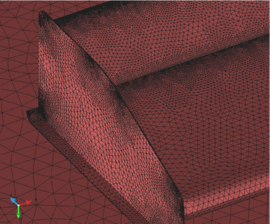
|
| (a) | (b) |
| Figure 50: Race car test – details of the finer mesh. | |
Again, five time steps are simulated, using a time step of . Between and processes were used for the tests. A summary of the times and iteration counts measured is presented in Table 6 for the million element mesh. As in the previous case, we observe a different behavior for the first iteration, due to the fact that it includes the time required to build and allocate the data structure of the system matrix and vector. In this case, the solution required less iterations to converge to the desired tolerance and, unlike in the previous case, no convergence problems were detected in the solution of the linear system. As a result, no distinction will be made between the results on the last time step and those on the previous ones. However, we do note that the first iteration requires significantly more time to solve the system than subsequent ones, specially for low process counts. As before, we consider this a consequence of the fact that the initial condition used is a bad approximation to an equilibrium solution.
| MPI processes | ||||||
| Assembly time | ||||||
| Solution time | ||||||
| Num. of iterations | ||||||
| Assembly time | ||||||
| Assembly speedup | ||||||
| Solution time | ||||||
| Solution speedup | ||||||
| Assembly time | ||||||
| Assembly speedup | ||||||
| Solution time | ||||||
| Solution speedup | ||||||
| Global speedup | ||||||
The parallel efficiency, in terms of strong scalability, is presented in graphical form in Fig. 51. The finite element procedure shows good scalability up to processors, where increasing times the number of processors reduces the assembly time by a factor of . This simulation, which corresponds to around thousand elements per process, gives us an upper limit to the scalability of the current implementation since, from this point on, increasing the number of processes does not result in a reduction of the assembly time. The system solution follows a similar trend, since in this case the solution time is actually increased when the number of processors is doubled from to .
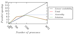
|
| Figure 51: Race car test – parallel speedup for the million elements. |
The same test was simulated using the million element mesh and the measured times are reported in Table 7. Some snapshots of the obtained velocity field are shown in Fig. 52, to provide an idea of the mesh resolution and the nature of the solution after five time steps. We observe that, with a larger model, we do not reach the limit of the parallel implementation as in the previous case, although the parallel performance does drop slightly for the cases with more processors.
| MPI processes | ||||||
| Assembly time | ||||||
| Solution time | ||||||
| Num. of iterations | ||||||
| Assembly time | ||||||
| Assembly speedup | ||||||
| Solution time | ||||||
| Solution speedup | ||||||
| Assembly time | ||||||
| Assembly speedup | ||||||
| Solution time | ||||||
| Solution speedup | ||||||
| Global speedup | ||||||
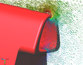
|
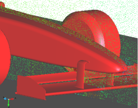
|
| (a) | (b) |
| Figure 52: Race car test – details of the velocity solution on the finer mesh. | |
The relative costs of the finite element assembly and solution phases are shown in Fig. 53. As in the inflatable structure test, we see that the solution represents takes the lion's share of the computational time and will have the most impact on the overall performance of the code. Again, we see that the first solution step has a significantly increased cost due to the additional operations and poor scalability, although the drop in parallel performance is not so severe as in the previous example.
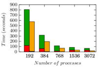
|
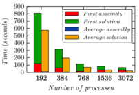
|
| (a) 12 million element mesh. | (b) 102 million element mesh. |
| Figure 53: Race car test – time costs of a single iteration. | |
The strong scalability results of the million element case are presented in graphical form in Fig. 54. As was already mentioned, we do not observe the same drop in parallel performance as in the smaller model, due to the fact that here we have 8 times more elements per process. The assembly phase shows good performance up to the largest test, where the reduction in time is less than would correspond to the increase in processors, but the overall performance continues to be dictated by the system solution costs. The system solution shows good parallel performance in all cases.
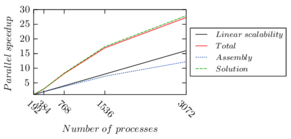
|
| Figure 54: Race car test – parallel speedup for the million elements. |
We also estimated the weak scalability in this case, keeping in mind that it is an optimistic estimate for the solve phase, since the increase in the number of processors is slightly larger than the increase in the number of nodes (which changes by a factor of in this case). The results are presented in Table 8 and coincide qualitatively with what was observed for the inflatable structure case. The build phase shows good weak scalability, close to one (although it drops somewhat in the vs. process comparison), while the solver has a poorer performance.
| Time ratio (fine problem/coarse problem) | ||
| Average assembly time ratio | ||
| Typical solution time ratio |
4.6 Computation of statistical data on a parallel environment
In the present work it has often been necessary to record statistics of turbulent flows. Sometimes this has been challenging, due to the amount of data to be analysed and to the parallel environment in which the simulations have been run, which has made necessary the synchronization of data across processes.
To understand the problems posed by the calculation of statistical results, consider for example the unbiased estimator of the variance of a random variable obtained using samples, given by
|
|
(4.270) |
where is the estimate of the mean of obtained using samples,
|
|
(4.271) |
The naive approach to the computation of the variance of involves two loops over the data series: a first one using Eq. 4.271 to obtain and a second one to evaluate Eq. 4.270. To do so, one should store the entire dataset and analyse it as a post-process. Take as an example the turbulent channel flow simulations using linear hexahedral elements. To record statistical data on this problem, the different values of interest were sampled on the integration points of the mesh. Using second order Gaussian integration we have 8 Gauss points per element. With up to hexahedra, we obtain samples per variable and time step. Keeping in mind that we want to calculate statistics involving all three velocity components, pressures and their gradients, storing the entire data set soon becomes very expensive in terms of memory.
Even if that data was effectively collected, consider that we used it to compute plane averages. In a parallel environment, the integration points on a given plane will likely lie on multiple processes, so the entire data set for the plane has to be gathered on a single process in order to evaluate Eq. 4.270.
When calculating the variance, one might compute it without storing the entire data series by manipulating Eq. 4.270 to obtain
|
|
(4.272) |
which can be calculated in a single pass, thus avoiding the need to store the data series. Unfortunately, this expression runs into numerical roundoff errors if . This is easy to see if one considers that in this case, can be expected to be a small number for each individual term in the summation of Eq. 4.270, while both and will be large positive numbers, so their difference might have too few significant digits1.
Instead, we have followed the approach of [89], which provided formulas to compute the mean and variance of a data set given the means and variances of two sub-sets of the data. A similar procedure is presented for third and fourth order moments in [90] and generalized to arbitrary order moments in [91]. These formulas allowed us to calculate statistical results in a single pass, storing (and communicating across processes when needed) only a partial result for each statistic.
(1) There are ways around this issue. For example, one could use an auxiliary variable , where is a crude approximation of the mean, to reduce roundoff error.
4.6.1 Mean and variance
Consider a set of samples divided into two arbitrary subsets , , containing and elements respectively, such that and . The means of , and are related by
|
|
|
|
defining we can write
|
|
(4.273) |
Eq. 4.273 can be introduced in Eq. 4.270 to obtain a single pass formula for variances. Introducing the intermediate result ,
|
|
(4.274) |
Now we can develop the first term on the last line
|
|
where we have used the definition of to say in the last step. The same reasoning can be used on the second term on the last line of Eq. 4.274 to obtain
|
|
Going back to Eq. 4.274, we can use the fact that to write
|
|
from here we can obtain the desired expression, given in [92], which is
|
|
(4.275) |
In practice, it is convenient to store the sum of all terms as an intermediate result instead of the mean. Defining , Eq. 4.275 can be rewritten as
|
It is useful to particularize this expression for the case , , which corresponds to adding a new measurement, , to the data set
|
We can keep track of as many partial results as needed by storing , and for each subset and using Eqs. 4.278 and 4.279 to update them. Once the calculation is finished and, for parallel simulations, any distributed data is gathered, the partial results can be combined using Eqs. 4.276 and 4.277 and the mean and variance of the complete record is recovered by
|
|
(4.280) |
4.6.2 Covariances
The present approach was extended to covariances in [91]. The covariance of two random variables , with means , can be estimated from realizations of as
|
|
(4.281) |
which again requires a previous estimate of the mean of each variable.
We can obtain a single pass formula for the covariance using a similar procedure to that followed for variances in the previous section. We define the intermediate result and use Eq. 4.273 to write and in terms of the partial results in Eq. 4.281. After rearranging the resulting expression, we obtain
|
|
(4.282) |
which can be particularized for the case where , as
|
|
(4.283) |
4.6.3 Third order statistics
The third order central moment of a distribution can be estimated from samples as
|
|
(4.284) |
It can also be calculated in a single pass by means of the following formula, taken from [90]:
|
|
(4.285) |
In the present work, we have not used third order central moments, but the turbulence energy budget involves correlations between three different variables (two velocity fluctuations and a gradient). Triple correlations can be estimated using the general expression
|
|
(4.286) |
which again can be transformed into a single-pass formula by using Eq. 4.273 to write the different means that appear in Eq. 4.286 in terms of the partial means in each subset. Rearranging the terms and introducing the partial result produces the final expression
|
|
(4.287) |
Using Eq. 4.287, we can evaluate any triple correlation in a single pass, provided that we also keep track of the pairwise covariances and individual averages of each variable involved in the calculation. Fortunately, in the present work we were already interested in these quantities, as they appear in other terms of the turbulence energy budget, and this did not suppose an additional cost.
Finally, the particular case , results in the following simplified expression
|
|
(4.288) |
4.7 Concluding remarks and future work
The parallelization of an existing code is a challenging task and requires significant efforts, some of which we presented here. As a general remark, it is important to design the code to be parallel from the start, choosing algorithms that require a minimum amount of parallel communication by design, rather than just parallelizing existing algorithms. This is particularly important in the choice of linear solvers, both because of the large impact the solution has in the total cost of the problem and because traditional approaches such as direct or Krylov solvers tend to parallelize poorly due to their communication requirements. We saw another example of this in the techniques for the calculation of flow statistics the algorithms of Section 4.6, where a specially designed technique is much more appropriate than the naive approach.
From the point of view of the parallel design of the code, Kratos Multiphysics currently uses blocking communication operations, in which execution of the code stops while data is being transferred between processors. Newer versions of MPI allow non-blocking communication, in which the data to be sent is defined and calculations can continue while communication goes on in the background. This could allow significant time savings for all calculations that can be written in a way where sent data is not immediately required in the receiving process.
Another addition that is being considered is the use of hybrid parallelization, based on combining a distributed approach such as the one presented here with a shared memory implementation. This could be potentially useful in machines such as the Gottfried cluster we used for our tests, where each calculation node contains multiple processors with a shared memory. In this situation, hybrid parallelization would allow us to use MPI for inter-node communication and simpler shared memory parallelization for the processors within the node.
Finally, we have devoted some time to describe our approach to partitioning the calculation mesh in Section 4.3. While this effort is essential for the initial subdivision of the domain, it is not sufficient when the calculation mesh changes during the problem, something that will happen in Chapter 5. When this happens, an approach for dynamic re-balancing of the problem would be required, reassigning nodes and elements to ensure that the computational load on each process remains homogeneous during the entire simulation.
We want to remark that the techniques and results presented in this chapter represent some recent developments in the parallelization of the Kratos Multiphysics FEM framework and are a part of an ongoing work. In this sense, they should be understood as a snapshot of some recent developments rather than a finished result. This is particularly true for the numerical results presented in Section 4.5 as AMGCL, the solver library we are using, is still under active development.
5 Adaptive mesh refinement for turbulent and viscoplastic flows
5.1 Introduction
One of the main advantages of finite elements is the possibility of using unstructured meshes, adapting the element size to the features of the problem and using finer resolutions near regions of interest. This requires a certain degree of familiarity with the problem being solved, as an insufficient mesh resolution can lead to missing important features such as boundary layers or sharp changes in the solution. In this sense, it would be desirable to have the ability to adaptively modify the mesh during the simulation, ensuring that its resolution is sufficient to represent the solution with a given accuracy at all times.
The first problem related to this strategy is how to quantify the error in the solution. One popular approach to this question are a posteriori error estimation techniques (see for example [93,94,95,96]), where the computed solution itself is used to assess its accuracy. We explore one of such methods, closely related to the VMS stabilized formulations introduced in Chapter 2, which was originally presented in [97] for convection-diffusion problems and has been applied to the Navier-Stokes equations in [98,99].
Once we are able to estimate the error and its distribution across the domain, we can modify the calculation grid to increase the overall accuracy. Many different mesh modification strategies have been proposed since the pioneering work in the late eighties [100,101,102], involving for example local mesh modifications [103], movement of mesh nodes through the solution of an auxiliary elasticity problem [104], mesh morphing techniques [105] or edge stretching [106]. However, mesh refinement, and meshing in general, is a particularly challenging problem in a distributed memory setting, as maintaining mesh quality over the entire domain and ensuring that the mesh is conforming is a very non-local problem, requiring communication across the different parallel subdomains. We propose a mesh refinement algorithm based on edge division that was designed with parallel performance as its main goal, requiring as little information that is not local to each element as possible.
Our mesh refinement strategy was originally conceived as a complement to the incompressible fluid solver of Chapter 2, with the goal of increasing the reliability of the solution and optimizing the number of elements for the simulation of large turbulent flow problems with meshes in the LES range. However, during the development of the present work, an opportunity appeared to use the same approach in the simulation of viscoplastic fluids.
Viscoplastic fluids are a class of non-Newtonian fluids that are rigid unless the applied shear stress is larger than a threshold, known as the yield stress. We concentrate our attention on Bingham fluids in which, once the material starts to flow, shear stress varies linearly with strain rate increments. Adaptive mesh refinement techniques, involving full remeshing of the domain, have been used in the past to simulate plane and axisymmetric Bingahm fows [107,108,109] and also to simulate depth-integrated free surface flows using a shallow water approximation [110]. We will apply our approach to the simulation of both plane and fully tri-dimensional cases.
The present chapter is organized as follows: first, the complete refinement procedure and its parallel implementation are presented in Section 5.2, followed by their application to incompressible flows in Section 5.3. Section 5.4 introduces the solver used for the simulation of non-Newtonian flows, which is applied to the simulation of Bingham fluids in Section 5.5. Some final remarks and conclusions are given in Section 5.6.
5.2 Adaptive refinement strategy
The refinement procedure we use is based on creating new elements by edge division. New nodes are inserted on edge mid-points of elements where the solution is considered to have a too large error. Once the new nodes have been added, the mesh is adapted to include the new nodes by subdivision of the existing elements. This approach involves several clearly differentiated components, acting in succession:
- An a posteriori error estimator to identify regions of the model that require refinement.
- A global refinement procedure that identifies the elemental edges to be divided and creates the new nodes.
- A local refinement technique to divide existing elements according to the patterns defined by the new edges and nodes.
In some examples we have considered one additional step, using local mesh improvement techniques to minimize the distortion of the elements in the new mesh.
It is important to note that the error estimation and the mesh refinement technique are independent of each other. This would allow us to combine the error estimator we present with a completely different refinement strategy, such as a full remeshing using Delaunay triangulation. Conversely, the only input required by the mesh refinement strategy is knowing which elements must be divided. This means that it could be used in combination with a different error estimator. For example, by choosing an estimator not tied to VMS stabilization, we could use the same refinement technique in combination with the FIC solver presented in Chapter 3.
5.2.1 Error estimation
The error estimator we use is based on the ideas presented by Hauke et al. in [97] for fluid transport problems. The same approach was applied to the Navier-Stokes equations in [99] and in [98], where part of the material that constitutes this chapter was originally presented. This estimator is motivated by the scale separation introduced in VMS formulations, which we presented in Chapter 2 for Newtonian flows and will be used again in Section 5.5 to stabilize viscoplastic flows.
Considering that the large scale variables represent the part of the solution reproduced by the finite element mesh, and small scale variables represent the part that is not resolved, the later can be understood as a measure of the local error in the solution. Once the large scale flow has been solved, the small scale can be evaluated on chosen points in the domain and its magnitude can be used as an a posteriori error estimator, identifying regions where the mesh is too coarse.
Following this argument, we define the following estimate of the error in element , to be used in VMS stabilized formulations
|
|
(5.289) |
In the present chapter we are mainly concerned with the static versions of the ASGS and OSS methods, which will be briefly recalled. The small scale model for the static ASGS formulation was defined in Chapter 2 as
|
|
(5.290) |
while the corresponding model for the static OSS method was introduced as
|
|
(5.291) |
Replacing the small scale velocities in Eq. 5.289 by their definition we obtain the final expression for the estimator. Using Eq. 5.291, the OSS estimator can be expressed as
|
|
(5.292) |
On the other hand, for the ASGS formulation, we use the definition for the small scales given by Eq. 5.290. This leads to an expression that is equivalent to dropping the projection from Eq. 5.291.
To perform a refinement step we evaluate the error estimate on each element and identify those elements where the estimate is larger than a pre-defined tolerance. These elements are then split according to the algorithm described in the following section.
It is worth noting that multiple variants of a subscale based error estimator were presented in [97]. The version presented here corresponds to the case where no elemental boundary integrals are included in the indicator. We chose to do so to keep consistency with the actual small scale model we use in the calculations. The boundary terms in question appear when keeping the elemental boundary integrals in the derivation of the stabilized VMS formulation. Since we neglected these terms in our derivation (as was shown in Chapter 2), we will not take them into account here.
5.2.2 Mesh refinement strategy
The mesh refinement strategy we use is based on the local subdivision of existing triangles or tetrahedra by edge division. The procedure was designed to require only a minimal amount of information that is not local to the elements to be refined, in order to simplify its implementation in a distributed memory environment. The main idea of the refinement algorithm is that, once an element has been identified as a candidate for refinement, it is divided into new elements created by splitting the edges of the original element in half. Neighboring elements are then refined by splitting some of their edges as required to maintain consistency. The main steps of this procedure are shown graphically in Figure 55 and can be described as follows:
- Iterate over mesh elements, evaluating the error estimator of Eq. 5.289.
- If the error estimate is larger than a predefined tolerance in a given element, mark it and its edges as needing refinement (Fig. 55a).
- A new node is created in the mid-point of all edges that have been identified as needing refinement. All nodal data (and in particular initial guesses for velocity and pressure) is interpolated from the nodes that define the edge (Fig. 55b).
- All elements with refined edges are deleted. Note that this includes elements where the error estimator was not larger than the tolerance (Fig. 55c).
- New elements are created using predefined patterns (Fig. 55d).
Regarding the last step, the creation of new elements is done according to predefined subdivision patterns, based on which and how many edges of each triangle or tetrahedra were subdivided in Step 2.
5.2.3 Local refinement of triangles and tetrahedra
The mesh refinement strategy described in the previous section is based on inserting nodes on edge midpoints and subdividing existing elements to include the new nodes. Unfortunately, knowing only which edges to split in each tetrahedron is not enough to ensure that the resulting mesh will be conforming. Consider for example the two elements in Fig. 56, where two new nodes are inserted. There are two possible ways in which the common face can be divided, corresponding to the two tetrahedra in Fig. 56c. To obtain a conforming mesh, the splitting strategy has to be designed in a way that ensures that the division of each element results in conforming faces.

|

|

|
| (a) Original elements. | (b) Conforming division. | (c) Non-conforming division. |
| Figure 56: Division of tetrahedra based on edge splitting. | ||
This restriction is problematic in a distributed memory environment, as the elements involved might belong to different partitions. In such situation, obtaining information from the neighbor element is not straightforward and involves communication between the partitions.
To solve this issue, we use an approach that is based exclusively in the numbering of the existing nodes, which is both available locally in the partition and known to be identical across partitions, avoiding all parallel communication. We start by assuming that all the edges of the element are split by their midpoints, resulting in four smaller elements in the case of a triangle or eight in a tetrahedra. If a given edge is not divided, at least one of the new elements touching that edge is eliminated. An example of this operation, which we call a collapse, is presented in Fig. 57, in which the four potential elements obtained by the full refinement of a triangle are reduced to three.

|

|

|
| (a) | (b) | (c) |
| Figure 57: Collapse operations on a triangle: (a) no collapse; (b) edge collapsed towards node or (c) collapsed towards node . | ||
To choose between the two possible outcomes of the collapse, the global node indexes of nodes and are compared. The partitioning in Fig. 57b is adopted if the index of node is smaller and the division of Fig. 57c is used otherwise. When subdividing two tetrahedra that share a face, using this criterion ensures that the subdivisions obtained from each element will be conforming. It must be noted that this approach has the obvious drawback of not taking the quality of the refined elements into account, but on the other hand it is purely local and therefore easily parallelizable.
Using this strategy we can determine the shape of the refined triangles or, in the case of a tetrahedron, the way in which its faces will be refined. For tetrahedra, the volume is then divided according to predefined patterns, depending on the shape of its faces.
The splitting operation defines three possible situations on each edge of the tetrahedron, corresponding to the three cases in Fig. 57. Given that there are six edges on each tetrahedron, up to potential face patterns can be defined. Each of those is matched to a division pattern using an utility1 distributed within Kratos Multiphyisics [29] which implements the local refinement operations. This tool, given an array containing the global indices for the nodes involved in the subdivision, divides the faces according to the collapse criterion and produces the connectivities for the new elements to be created. Note that, for some division patterns, a new node is added on the element's center of mass to improve the quality of the resulting elements. A very important point to be made here is to consider how this procedure affects mesh quality. If all edges of an element are divided, the refinement procedure ensures that its quality is preserved, as all new elements have the same angles as the original in this case. Unfortunately, this is not the case for elements where only some of the edges are refined, and mesh quality can be significantly degraded if this kind of partial refinement is performed repeatedly over the same patch of elements. To alleviate the problem, we improve the quality of the resulting mesh using local mesh improvement techniques. For simulations, we used the algorithm presented in [111], which is based on reconnecting the nodes of adjacent elements. For cases, we used the procedure presented in [112], which consists in analyzing clusters of adjacent elements and changing the local topology, adding or deleting nodes and reconnecting elements to improve mesh quality within the cluster. As these techniques were incorporated in the code on a late stage in the presented work, they were not used for the turbulent flow cases. However, we took full advantage of them to simulate the Bingham flow cases presented in Section 5.5.
(1) The source code that provides this functionality can be found in the address https://kratos.cimne.upc.es/projects/kratos/repository/changes/kratos/kratos/utilities/split_tetrahedra.h (retrieved on July 22, 2015).
5.2.4 Parallel implementation
The proposed mesh refinement strategy has been implemented for a distributed memory environment within the Kratos Multiphysics framework. This means that the domain partitioning model introduced in Chapter 4 is also used here. Individual elements are assigned to a single parallel subdomain and are completely unknown by the others. Nodes are also assigned to a subdomain, which holds the reference values for all data associated to that node, but might be also needed in neighboring domains if they are connected to elements lying on different partitions. When this happens, other partitions store a copy of the nodal data, which has to be updated at different points during the simulation. From the point of view of a given subdomain, nodes are said to be local nodes when that subdomain holds the reference values for their data or ghost nodes otherwise. Our implementation of the refinement strategy relies on an auxiliary sparse matrix that reproduces the edge connectivity pattern of the mesh. As in Chapter 4, we rely on the implementation of sparse distributed memory matrices provided by the Trilinos library [80] to define and store it. We consider a simplified scenario to clarify the presentation of the algorithm. Consider an initial finite element mesh containing nodes and elements divided in subdomains. The nodes are numbered consecutively in the range and ordered by subdomains, such that, if a node is local to subdomain , its index will be in the range . We remark that this is done to simplify the notation used to describe the implementation, but it does not represent a restriction on the actual implementation. In practice we only assume that the nodes are numbered sequentially as a whole, even if consecutive nodes are not in the same partition. Additionally, we denote the edges of finite elements in the mesh as pairs of node indices , with . We define a sparse matrix of size representing the edge connectivity pattern. Position can only be different from zero if there is some elemental edge joining nodes and . Note that, using our definition of the edge, only contains terms above its diagonal. Matrix is stored using compact storage by rows (CSR) notation and distributed, meaning that each parallel process stores non-zero terms for rows in the range . Note that the process will sometimes need to access rows outside this range, corresponding to ghost nodes in the partition, an operation that requires parallel communication. In the following we refer to the set including all local and ghost nodes known to partition as . The implementation of the refinement algorithm involves multiple tasks that can be grouped into the following steps:
- Build a sparse matrix of edge connectivities , where position of the matrix only exists if there is an element edge joining nodes and in the mesh. Positions corresponding to an edge are initialized to the arbitrary value -1. This is represented in pseudo-code in Algorithm 4. Note that, as the matrix is defined as upper-triangular only the positions where are considered.
|
|
Algorithm. 4 Initialization of the matrix of edge connectivities . |
- Iterate over the elements, checking if they should be refined. If an element is identified as needing refinement, set the positions corresponding to its edges in to -2 (Algorithm 5). Note that this step requires parallel communication to ensure that edge data is consistent on all subdomains.
|
|
Algorithm. 5 Identification of edges to refine. |
- The number of new nodes to be added in each subdomain is equal to the number of -2 entries in all known rows of . Use this information to assign a range of temporary node indices , to each process (Algorithm 6). Some new nodes will be counted twice, as they are known by multiple domains.
|
|
Algorithm. 6 Definition of temporary node ranges for process . |
- Each process claims ownership of known new nodes by assigning it node index in its range. Note that this process will sometimes produce clashes, as nodes in the interface between subdomains are known by multiple processes (Algorithm 7). We decided to allow overwriting node indices set by other processes, so that the last process to assign an index will own the node.
|
|
Algorithm. 7 Definition of node ownership. |
- Each process creates new nodes locally on edge midpoints (Algorithm 8). Nodal data is initialized by averaging the values stored by the nodes on both ends of the edge. The new node must be created on all partitions that know it, independently of which process owns the node, as node ownership only determines which process holds the reference data during synchronization.
|
|
Algorithm. 8 Creation of new nodes. |
- Create new elements locally using the subdivision procedure described in Section 5.2.3 (Algorithm 9). Note that all elements with one or more refined edges must be subdivided, not just those identified using the refinement criteria. Recall that, in , new nodes can be created at the element center in some cases, to avoid creating highly distorted elements. If this happens, the node is created as local to the partition that owns the element and its nodal data is interpolated from the nodes of the original tetrahedron.
|
|
Algorithm. 9 Creation of new elements. |
- The procedure used to assign new nodes, combined with the fact that new nodes can be unexpectedly created during elemental subdivision, means that the final node numbering might not be consecutive or, worse, contain duplicate indices. This is also an issue with elements: as original elements are erased there will be gaps on the element numbering. Renumber nodes and elements across processes so that indices are unique and consecutive again.
- If desired, the local mesh improvement procedure mentioned in Section 5.2.2 can be used as a post-process to increase mesh quality at this point.
- Finally, the communication strategy used to synchronize nodal data must be redefined to account for new nodes created on interface edges. This is done using the coloring procedure described in Chapter 4.
5.2.5 Scalability test
As a first test of the refinement algorithm and its parallel implementation we refined a tetrahedral mesh homogeneously. We define a cubic domain given by its corners and and generate an initial mesh composed of slightly over one million tetrahedra. This mesh, as all initial meshes used in later examples, has been generated using the pre-processing module of GiD [77]. The domain is fully refined in two passes, first splitting all elements to obtain about million tetrahedra and again for a total of million elements. The local mesh improvement strategy is not used in this case, as we are interested in testing the implementation of the refinement algorithm and its performance. Times required to complete this operation using different amounts of parallel processes is recorded in Table 9. Reported times were obtained using up to three Intel Xeon E5645 processors, each consisting in two six-core CPU at connected to RAM each. Communication between processors was done through an Infiniband connection. The results are also presented in graphical form in Fig. 58.
| First step | Second step | |||
| Num. procs. | Wall time (s) | Speedup | Wall time (s) | Speedup |
| 4 | 21.16 | 1.0 | 170.74 | 1.0 |
| 8 | 10.57 | 2.0 | 88.09 | 1.9 |
| 16 | 5.71 | 3.7 | 48.99 | 3.5 |
| 32 | 3.25 | 6.5 | 24.99 | 6.8 |
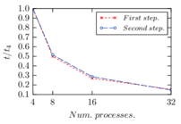
|
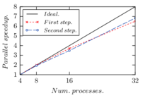
|
| (a) Relative wall time. | (b) Parallel speedup. |
| Figure 58: Homogeneous refinement test – parallel performance. | |
While the test results show good parallel performance, it must be remarked that this experiment does not take into account an important aspect in practice: when refinement is not homogeneous, the number of elements in each subdomain changes and, without a load balancing strategy, parallel performance may degrade as different processors can have very different loads if refinement is concentrated on a few of the original subdomains.
5.3 Application to laminar and turbulent flows
We simulated a first set of cases combining the incompressible fluid solver presented in Chapter 2 with the refinement algorithm introduced in the previous pages. All simulations were performed with the static OSS method, coupled with the corresponding error estimator, given by Eq. 5.292. With these tests, our aim was to test the applicability of our refinement strategy on distributed memory simulations, rather than obtaining high quality solutions.
5.3.1 Flow around a cylinder at 1005.3.1 Flow around a cylinder at
Re
=
{\displaystyle {\hbox{Re}}=}
100
As a relatively simple, small scale application we simulate the two-dimensional flow around a cylinder using static OSS stabilization. The set up of the problem, taken from [30], consists in a cylindrical obstacle of diameter centered on the origin of a domain defined by the range . A horizontal velocity is imposed on the left side of the domain, while a no-penetration condition is set on the top and bottom edges. The velocity is fixed to zero on the cylinder. The fluid properties are defined as and , such that the Reynolds number in terms of the diameter is . Starting from a uniform structured mesh containing linear triangles, seconds of flow are simulated using a time step of seconds. In this case, the refinement strategy is used after a starting phase to allow the simulation to transition from the initial condition to a dynamic solution. The refinement procedure is then used every 20 solution steps, resulting in a total of 40 refinement passes. The maximum number of refinements over a single original element is limited to 3 to preserve mesh quality and prevent excessive refinement on localized areas. Although the problem is small enough to be run on a desktop computer, the simulation was performed in a distributed memory machine, using 8 processes to test the parallel implementation. The initial mesh and the partition into parallel subdomains are shown in Fig. 59.

|

|
| (a) Initial mesh. | (b) Parallel subdomains. |
| Figure 59: Cylinder test – initial mesh and parallel partition. | |
|
|
| (a) Final mesh. | (b) Isolines of velocity magnitude. |
| Figure 60: Cylinder test – final mesh and velocity isolines. | |
From the point of view of load balancing, the element counts in Table 10 show that refinement is not homogeneous across subdomains and, at the end of the simulation, the largest domain has close to three times more elements than the smallest one. This suggests that the practical applicability of the method in a parallel context would be much greater if it included a dynamic load balancing strategy so that elements are always distributed evenly across subdomains.
| Process | 0 | 1 | 2 | 3 | 4 | 5 | 6 | 7 | Total |
| Initial | 496 | 510 | 501 | 493 | 494 | 490 | 505 | 495 | 3984 |
| Final | 1056 | 1871 | 836 | 740 | 1884 | 1694 | 1542 | 2043 | 11666 |
5.3.2 Flow around a 6 meter cube
Additionally, we studied a realistic three-dimensional case in order to test the refinement strategy on a tetrahedral mesh. We chose to simulate the flow around the Silsoe cube, a benchmark problem for the flow over bluff bodies. This test case reproduces an experiment performed at the Silsoe Research Institute [113] in which a cube with meter sides was placed under incoming wind. We simulate the configuration where the average wind direction is perpendicular to one of the cube faces. The cube is placed at a distance of from the inlet, while the incoming wind is defined according to the logarithmic wind profile of Eq. 5.293 (see for example [2]).
|
|
(5.293) |
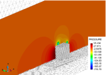
|
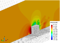
|
| (a) Pressure distribution at , original mesh | (b) Pressure distribution at , refined mesh |
| Figure 61: Silsoe cube – pressure results on the central plane and simulation meshes. | |
We observe that the refined elements are concentrated near the cube and its immediate wake. In the front of the cube, they are roughly placed along the area where the flow starts to deviate due to the obstacle. Experimental results show that a horseshoe vortex should develop close to the ground in that zone, and the distribution of elements seems to follow it. On the wake region, the refined area develops progressively as vortices detach from the cube and travel downstream. If the simulation was run for a longer period, it should be expected that the refined area would advance towards the exit to obtain a fully refined wake, as happened previously in the cylinder example. Finally, we want to remark that this simulation was performed to test the refinement algorithm in a realistic setting and not to obtain precise results. The Silsoe cube problem was analyzed using the same solver (without adaptive mesh refinement) in [114], obtaining good agreement with the benchmark solutions.
5.4 A FEM solver with adaptive mesh refinement for viscoplastic flows
The adaptive mesh refinement procedure presented in Section 5.2 can also be applied to the simulation of viscoplastic flows. For this we use a modified version of the VMS based solver presented in Chapter 2, adapted to the solution of the steady Navier-Stokes equations with non-Newtonian constitutive relations, which will be introduced here.
5.4.1 Model equations
Defining the fluid's velocity and density , the stress tensor and the external forces , the conservation of linear momentum can be stated as
|
|
(5.294) |
and the conservation of mass implies that, for an incompressible fluid,
|
|
(5.295) |
The definition of the problem is completed by introducing a model domain with boundary and appropriate boundary conditions
|
where is the imposed velocity on the Dirichlet boundary , is the outwards unit normal on the Neumann boundary and are the imposed tractions. The stress tensor of Eq. 5.294 can be decomposed into a volumetric part involving the pressure and a deviatoric stress tensor :
|
|
(5.298) |
where is the second order identity tensor. A constitutive model is required to close the formulation, giving an expression for the deviatoric stresses . A broad class of fluid materials follow a generalized Newtonian law given by
|
|
(5.299) |
where the apparent viscosity is, in general, a variable that depends on the characteristics of the flow and is the strain rate tensor, defined as
|
|
(5.300) |
Additionally, it is convenient to introduce the following tensor invariants to measure the magnitude of the strain rate and deviatoric stresses
|
|
(5.301) |
In the present work, a regularized Bingham model will be used. A Bingham fluid [115,116] is a material that remains rigid while the applied shear stress is lower than its yield stress . Once this limit is reached, the material starts flowing with a constant viscosity , the plastic viscosity. This can be expressed using the notation of Eq. 5.299 if the apparent viscosity is defined as:
|
|
(5.302) |
Unfortunately, the discontinuous nature of the Bingham model introduces numerical difficulties, as the apparent viscosity is infinite for small strain rates that don't produce flow. As a way to prevent this issue, we have adopted the regularized equation proposed by Papanastasiou [117], replacing Eq. 5.302 with
|
|
(5.303) |
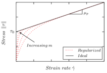
|
| Figure 62: Bingham model. |
5.4.2 Stabilized formulation
To introduce the variational form of the problem we define spaces and containing the exact values and , respectively, of the solution of the problem in . Additionally, we define the test functions , , where is defined as restricted to the zero Dirichlet condition on . The variational form of the problem can be obtained by multiplying Eqs. 5.294 and 5.295 by test functions , and integrating over the simulation domain :
|
where some terms have been integrated by parts. As seen in the previous chapters, the Galerkin weak form of the Navier-Stokes equations suffers from stability issues. In this case, we used the static versions of both the ASGS and OSS formulations to stabilize it. The choice of using a VMS based formulation has an added benefit: it allows us to use the error estimator presented in Section 5.2.1 without modification. We introduce the discrete solution as , , where and are the discrete spaces defined by the finite element interpolation. Given these definitions, the VMS approach is based in decomposing the problem variables into a large scale part, identified with the finite element solution, and a small scale part:
|
|
(5.306) |
where the small scale variables , represent the part of the continuous solution that is not resolved with the discrete interpolation. Next we introduce the scale separation of Eq. 5.306 in the variational problem given by Eqs. 5.304 and 5.305. Using test functions belonging to the discrete space , , we obtain
|
where represents a single element. Note that, to obtain this expression, we integrated by parts over individual finite element domains to ensure that the equations only involve the small scale values and not their spatial derivatives. In doing so, we neglected all integrals over element boundaries. Using ASGS stabilization, the model for the small scales is defined as
|
where and represent the residuals of Eqs. 5.294 and 5.295 respectively, evaluated using only the large scale part of the solution , . The stabilization parameters , are defined in terms of a characteristic element length as:
|
|
(5.312) |
When using OSS stabilization, only the part of the residuals and that is orthogonal to the finite element space is used to stabilize the solution. This results in the following modified model for the small scales:
|
where and are the projections of the residuals onto the finite element space, that is, the solution of the auxiliary projection problem
|
It is worth mentioning that the viscous term in Eqs. 5.310 and 5.313, as well as in the momentum projection in Eq. 5.315, cannot be evaluated using linear finite elements, as is the case of the formulation used in the present work. This is due to the fact that second order derivatives of velocity shape functions are identically zero within the elements. Therefore, this term will be neglected in the following. Introducing the OSS small scale model into the variational form of Eqs. 5.307 and 5.309, the following stabilized formulation is obtained:
|
|
(5.317) |
|
|
(5.318) |
Analogously, the ASGS stabilized formulation can be recovered by dropping all terms involving and in Eqs. 5.317 and 5.318.
5.4.3 Matrix formulation
At this point we can use the standard linear finite element functions to interpolate the large scale velocity and pressure solutions using nodal shape functions :
|
|
(5.319) |
where is the node index and the total number of nodes, represents the standard finite element functions for scalar variables and its matrix equivalent for vectorial quantities. Introducing the interpolation of Eq. 5.319 into Eqs. 5.317 and 5.318 and successively using the shape functions of each node as test functions , , we obtain the following system of equations
|
|
(5.323) |
where and represent the vectors of nodal values for velocity and pressure, respectively. The blocks that appear in the system matrix and the right hand side vector of Eq. 5.320 are obtained from the finite element assembly of the different integrals that appeared in the stabilized equations. If and represent node indices, the Galerkin terms in Eqs. 5.317 and 5.318 give rise to the following local matrices:
|
|
(5.324) |
Analogously, the discretization of the stabilization terms allows us to write
|
|
(5.325) |
The system in Eq. 5.320 contains multiple non-linear terms: the convective term is non-linear in the velocity, as are all terms involving either the apparent viscosity , the stabilization parameters , and, in the OSS formulation, the projections. To linearize it we use Picard iterations, evaluating all terms in the local contributions using the last known values of the variables and solving the system iteratively. In the case of OSS stabilization, an associated problem has to be solve to calculate the projections, given by the discrete form of Eqs. 5.315 and 5.316:
|
|
(5.326) |
where and represent the vectors of nodal values for the momentum and mass projections, respectively, and the different terms in the matrix and right hand side vector can be obtained by the finite element assembly of the following local contributions:
|
|
(5.327) |
Note that, as was done in previous chapters, we use the fact that the projection matrices and have the structure of a mass matrix to approximate them by the corresponding diagonal mass matrix. This avoids the solution of the linear system which would otherwise be required to obtain the projections.
5.5 Application to Bingham fluids
The formulation introduced in the previous section can be combined with the adaptive mesh refinement procedure by introducing the small scale model of Eq. 5.310 for ASGS simulations, or Eq. 5.313 for OSS, in the error estimator of Eq. 5.289. We have used it to simulate several classical examples of Bingham flow problems. As in the previous examples, GiD is used to generate the initial mesh. Here all examples considered are small enough to be computed in a desktop computer and, as a result, the distributed memory capabilities are not relevant. In all examples but the Poiseuille flow, local mesh improvement is used to correct the refined mesh.
5.5.1 Poiseuille flow
The first test case is a simple Poiseuille flow under an imposed pressure gradient. We define a plane channel and prescribe a pressure variation between its extremes as shown in Fig. 63. A no-slip condition is imposed along the edges of the channel. The fluid density is set to while the plastic viscosity takes a value of and the regularization coefficient is set to . We consider two cases: a Bingham flow with yield stress and a Newtonian case with viscosity .
|
| Figure 63: Poiseuille flow – geometry and boundary conditions. |

|
| Figure 64: Poiseuille flow – initial mesh. |
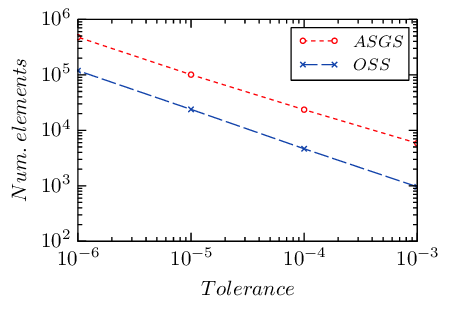
|
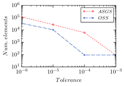
|
| (a) Newtonian fluid. | (b) Bingham fluid. |
| Figure 65: Poiseuille flow – number of elements at the end of the simulation for different tolerances. | |
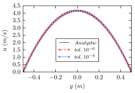
|
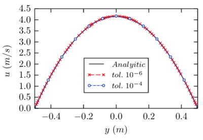
|
| (a) Newtonian fluid (ASGS). | (b) Newtonian fluid (OSS). |
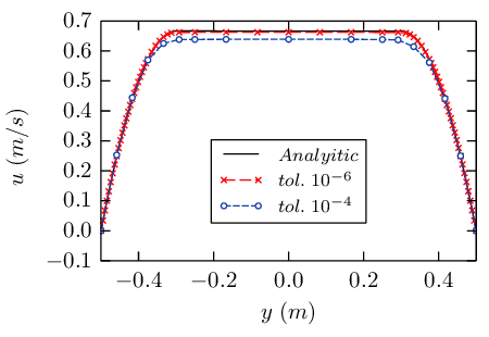
|
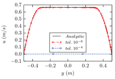
|
| (c) Bingham fluid (ASGS). | (d) Bingham fluid (OSS). |
| Figure 66: Poiseuille flow – streamwise velocity profiles. | |
Analyzing the results, we observe a different behavior for the two cases considered. In the Newtonian case, the number of elements in the final grid increases uniformly as the tolerance is reduced. This is in agreement with the expected behavior of the estimator used: consider the that analytical solution of the Newtonian Poiseuille flow is a parabolic velocity profile given by the expression
|
|
(5.328) |
where is the channel width and is the vertical distance to the lower wall. Consider the solution obtained using the ASGS stabilization. Assuming we obtained a nodally exact solution, the momentum error would be
|
|
(5.329) |

|

|
|
| (a) Initial mesh. | (b) Newtonian fluid. | (c) Bingham fluid. |
| Figure 67: Poiseuille flow – detail of the final meshes for the OSS case with tolerance . | ||
On the other hand, in the Bingham case the profile has an unyielded central area that moves as a block and two yielded regions close to the wall with a parabolic velocity profile. The central area, with constant velocity, can be solved with practically no error with a coarse mesh size, and most of the new elements are placed in the yielded regions. As the refinement is more localized, the overall number of elements is smaller. As a final remark, we can observe that, for small tolerances, the refinement fails to start if the mesh is too coarse to properly represent the flow. This can be seen in in Fig. 65b for the ASGS simulation with a tolerance of and for the OSS cases with tolerances and , where no new elements are added. These cases produce a solution where the yielded regions do not develop and the velocity is practically zero everywhere.
5.5.2 Plane extrusion
We simulated the plane extrusion of a Bingham fluid through a die with a 3 to 1 reduction of the cross-section. This problem, presented in [121], was also solved in [122], using a fixed fluid mesh and an ASGS-based solver similar to that of Section 5.4, and in [123], using OSS stabilization. As can be seen in Fig. 68, we use symmetry to simulate only one half of the domain. The walls are assumed to be smooth, and only the wall-normal component of velocity is restricted. The flow is driven by a ram pressure applied on the left side of the domain, which introduces a pressure gradient. The fluid parameters are reported in Table 11.
|
| Figure 68: Plane extrusion – geometry and boundary conditions. |
| Parameter | Value |
| Fluid density | |
| Yield stress | |
| Fluid viscosity | |
| Regularization coefficient |
As discussed in [121], using the present settings, with smooth walls and a very small plastic viscosity, the problem is analogue to a perfect plasticity problem. An exact solution for the plasticity problem, obtained using slip line theory, is reported by Lubliner in [124]. This solution predicts the formation of slip lines once the applied pressure reaches
|
|
(5.330) |
|

|
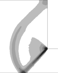
|
| (a) . | (b) . | (c) . |
|
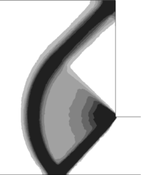
|
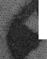
|
| (d) . | (e) . | (f) . |

|
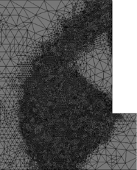
|

|
| (g) . | (h) . | (i) . |
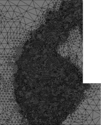
|

|
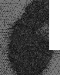
|
| (j) . | (k) . | (l) . |

|
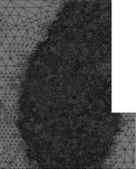
|

|
| (m) . | (n) . | (o) . |
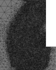
| ||
| (p) . | ||
| Figure 69: Plane extrusion (ASGS) – evolution of strain rate (left) and mesh (right). | ||

|

|

|
| (a) . | (b) . | (c) . |
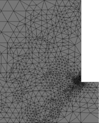
|
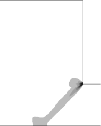
|
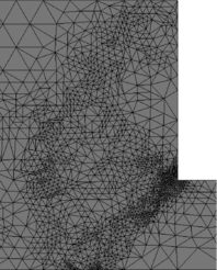
|
| (d) . | (e) . | (f) . |
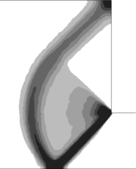
|
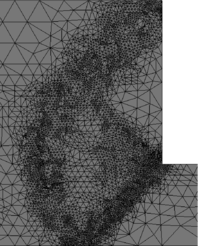
|

|
| (g) . | (h) . | (i) . |
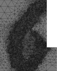
|

|
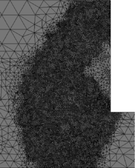
|
| (j) . | (k) . | (l) . |

|
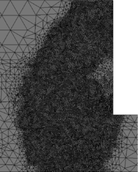
|

|
| (m) . | (n) . | (o) . |

| ||
| (p) . | ||
| Figure 70: Plane extrusion (OSS) – evolution of strain rate (left) and mesh (right). | ||
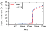
|
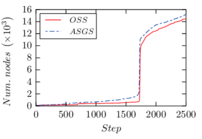
|
| (a) Number of elements. | (b) Number of nodes. |
| Figure 71: Plane extrusion – evolution of the simulation mesh. | |
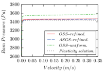
|
| Figure 72: Plane extrusion – applied pressure vs. inlet velocity. |
We can also observe in Fig. 72 that the OSS simulation predicts a slightly later plastification, corresponding to higher ram pressures, when compared to the ASGS method, while the latter is closer to the plasticity theory result. A possible explanation for this could be that the ASGS estimator produces a larger number of elements overall, as can be seen in Fig. 71, which provides a slightly better accuracy in the solution. As an attempt to quantify the effectiveness of the refinement procedure, we also simulated the problem using OSS and a uniform mesh containing elements, a similar amount as in the finest mesh obtained during the refinement, to use as a reference solution. The velocity–pressure relation for this simulation is also plotted in Fig. 72 and shows a delayed formation of the yielded region, which appears at higher ram pressures than expected. While using a uniform mesh would be a very naive approach in this case, the results show that the use of a refinement procedure results in an improved solution for a given number of elements in the mesh.
5.5.3 Cavity flow
The next example we considered is the 2D cavity flow of a Bingham fluid. The problem uses the same settings as Mitsoulis and Zisis in [125]. Defining a square domain , we impose a horizontal velocity on the side and zero velocity on the remaining sides. We simulate a leaky cavity, the top left and top right corner nodes have a fixed horizontal velocity. This condition is re-imposed after each refinement step, so that the wall node immediately next to the corner always has zero velocity, as shown in Fig. 73, even if this node didn't exist in previous iterations.
|
| Figure 73: cavity flow – boundary conditions. |
The fluid density is set to and the dynamic viscosity for the yielded region is set to . We will simulate multiple cases with different yield stresses to test a range of values of the Bingham number, defined as
|
|
(5.331) |
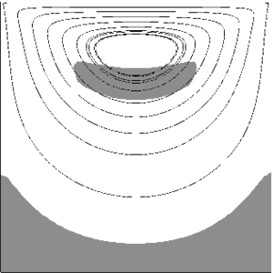
|
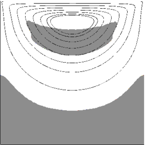
|
| (a) . | (b) . |
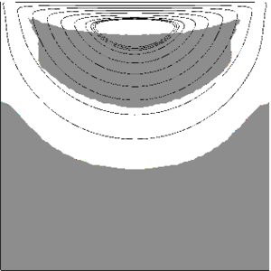
|
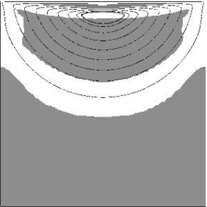
|
| (c) . | (d) . |
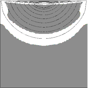
|
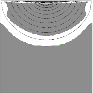
|
| (e) . | (f) . |
| Figure 74: cavity flow – velocity streamlines and distribution of yielded (light) and unyielded (dark) regions. | |
![2D cavity flow – vertical position of the vortex center, compared to the results of [125].](/wd/images/thumb/3/3d/Cotela_2016-cavity_center.png/216px-Cotela_2016-cavity_center.png)
|
| Figure 75: cavity flow – vertical position of the vortex center, compared to the results of [125]. |
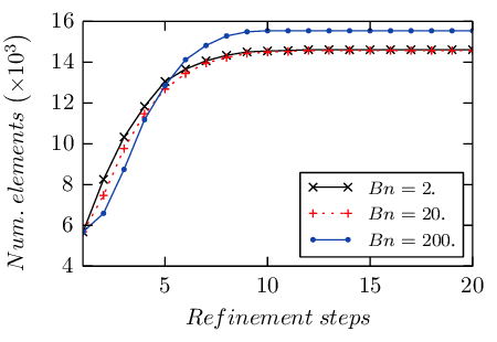
|
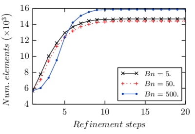
|
| (a) | (b) |
| Figure 76: cavity flow – evolution of the number of elements. | |
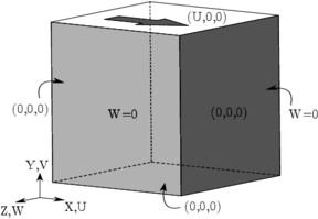
|
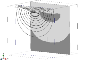
|
| (a) cavity flow – geometry and velocity boundary conditions. | |
| Figure 77: cavity flow – velocity streamlines and distribution of yielded (light) and unyielded (dark) regions. | |
The flow is simulated in 10 solution steps, refining after each solution. Starting from a uniform tetrahedral mesh with divisions along each edge, containing approximately thousand nodes and thousand elements, a final mesh with thousand nodes and thousand elements is obtained. The final distribution of yielded and unyielded regions and velocity streamlines is shown in Fig. 77. The vortex center in this case is placed at a vertical position , in agreement with the results shown in Fig. 75.
5.5.4 Flow through a sudden expansion
As a final test case we have simulated the flow through a square sudden expansion. This problem was studied in [127,128] for Herschel-Bulkley fluids and represents a three-dimensional version of the more common planar or axisymmetric expansions (see for example [129,130,131]). The cross section of the problem is shown in Fig. 78. We modeled the flow through expansions with 1 to 2 and 1 to 4 width ratios, which correspond to and using the notation of Fig. 78.
|
| Figure 78: Sudden expansion – geometry. |
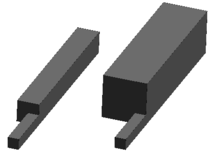
|
| Figure 79: Sudden expansion – simulation domains. |
The problem is solved for the case where both the Reynolds and Bingham numbers equal to one, calculated using as the reference length and a reference velocity defined in [127] as
|
|
(5.332) |

|

|

| |
| (a) Side view. | (b) – | (c) – | (d) – |
| Figure 80: expansion – yielded (dark) and unyielded (light) regions. | |||

|

|

|

|
| (a) Side view. | (b) – | (c) – | (d) – |
| Figure 81: expansion – yielded (dark) and unyielded (light) regions. | |||
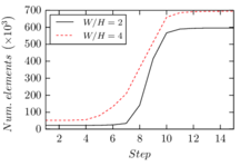
|
| Figure 82: Sudden expansion – evolution of the number of elements during the simulation. |
| (a) Initial mesh. | (b) Final mesh. |
| Figure 83: expansion – side view of the calculation meshes. | |
| (a) Initial mesh. | (b) Final mesh. |
| Figure 84: expansion – side view of the calculation meshes. | |
The initial and final meshes are shown in Fig. 83 for the test and Fig. 84 for the case. It can be observed that refined areas coincide with yielded regions, where higher velocity gradients are generally found: close to the solid walls and just after the expansion section.
5.6 Summary and conclusions
In the previous pages we have presented an adaptive mesh refinement technique that combines an a posteriori error estimator based on the VMS scale separation and a mesh refinement strategy based on edge division, designed and implemented to work in a distributed memory parallel environment. This approach has been applied to the simulation of turbulent and viscoplastic flows, improving the resolution of triangular meshes in and tetrahedral meshes in . To conclude the presentation, we will give some final thoughts on the method and propose future lines of improvement. We have shown that our approach to mesh refinement is parallel by design and its distributed memory implementation shows good parallel performance. This is achieved through the use of a very simple refinement procedure, based only on data that is local to the element. In fact, the division procedure presented in Section 5.2.3 is based only on the nodal numbering. The drawback of this approach is that the quality of the resulting refined mesh is not taken into account when dividing elements, which can result in a sub-optimal mesh quality. A local division strategy that took into account the shape of the element and its neighbors when refining could allow us to chose a more convenient division pattern in many cases, resulting in better mesh quality. This suggests a first venue for future improvement, for example devising an improved approach that incorporates the ideas of the local mesh improvement techniques we now use as a post-process to choose an optimal refined configuration, but always keeping in mind that the parallelization of such approach would have to be carefully considered. A second possibility for improvement of the mesh refinement strategy is the treatment of curved surfaces. While this has not been significant in the examples presented here (only the cylinder example included curved edges), a drawback of our refinement algorithm is that, when working with curved surfaces, the quality of their representation is given by the coarsest mesh used during the process. This issue is shown graphically in Fig. 85, and would likely be problematic in cases where a precise description of the geometry is required, such as flows around wing profiles or wind turbine blades, regardless of the final mesh size. A starting point to solve this issue could be storing the original geometry using, for example, a NURBS-based description and using this information to correct the position of new nodes, placing them closer to the original surface instead of on the edge midpoint.
|

|

|
| (a) Original domain. | (b) Coarse mesh. | (c) Refined mesh. |
| Figure 85: Refinement of curved edges. | ||
The incompressible flow examples presented in Section 5.3 allow us to say that our approach correctly identifies the zones where refinement is required. However, regarding the parallel efficiency of the method, we found that dynamic load balancing is necessary to solve large scale examples efficiently, as local refinement can quickly unbalance the original partitioning of the model. Additionally, mesh coarsening would be a welcome addition to solve dynamic problems as, in our experience, the regions with larger error tend to follow moving vortices and this currently results in a complete refinement of turbulent wakes. Although our adaptive refinement strategy was originally designed to simulate turbulent flows, we found that it is also suited to the simulation of viscoplastic fluids. The fact that many problems of interest in this field are generally static and have sharp interfaces between yielded and unyielded regions plays to the strengths of our approach, as coarsening is rarely required. We found that our method was able to identify the regions where fluidification occurs even when starting from a uniform initial mesh. While the capabilities of the method have been demonstrated by the test cases presented in Section 5.5, there are some questions that could be addressed in the future. For example, how should the tolerance for the error estimator be set? Is it problem dependent? In our experience, the solution is sensitive to the tolerance set for the error estimator: a small tolerance produces very fine meshes, while a large tolerance can even prevent the refinement from starting if the original mesh is too coarse. This was shown to be the case in some of the Poiseuille flow examples presented in Section 5.5.1. Going back to turbulent flow, there is one interesting question regarding the chosen estimator. According to the arguments presented in Chapter 2, the small scale part of the solution can be understood as the basic ingredient of a VMS-based turbulence modeling. In this sense, imposing a restriction on its magnitude seems to be contradictory with our goal in previous chapters, which was to perform a LES-like simulation thanks to the contribution of the small scale terms, and seems to push the mesh size towards DNS simulations, which we discarded as prohibitively expensive for problems of engineering interest.
6 Conclusions
6.1 Summary and main results
In the present work we have explored the capabilities of stabilized finite element formulations for the solution of turbulent flow problems. To achieve this goal, we have studied two families of methods: VMS and FIC formulations, applying them to the solution of different benchmark problems. In addition, we have studied numerical techniques relevant to the solution of large complex problems, in particular the parallel implementation of the code and the use of adaptive mesh refinement to improve the quality of the simulation mesh.
As a general observation for the different stabilized formulations considered, we noticed a notable difference between using linear tetrahedral or hexahedral finite elements in terms of the quality of the solution. While this was not unexpected, we were able to quantify the difference for the turbulent channel flow, where we see that, in general, we need an order of magnitude more tetrahedral elements to achieve the same quality in the solution as for hexahedra.
For VMS methods we have studied the behavior of classical formulations on the channel flow problem, in terms of velocity averages and variances and of the turbulence kinetic energy balance. Additionally, we have presented a new model for the pressure subscale based on the use of an approximate small scale space, which has been shown to provide a promising improvement in the quality of the solution for the channel flow test when compared to the usual approach. However, we want to remark that we consider this only a starting point, since the effect of the pressure small scale on the solution has been shown to be problem-dependent in the literature.
Regarding FIC formulations, introduced in Chapter 3, we have presented a new method that includes a diffusive term based on imposing the FIC balance in the direction of the gradients of each component of velocity, in addition to the usual streamline diffusion. Although this term is derived from the FIC balance (as opposed to a turbulence modeling argument), we have shown its presence allows us to obtain a more accurate solution in the turbulent channel flow benchmark. We have also applied the resulting formulation to more complex geometries, and in particular to the wind flow around a parabolic solar collector. While the simulation performed represents only a first approximation to the problem, as more tests and longer simulation times would be required to obtain a more reliable solution, they are encouraging in terms of the performance of the method.
In Chapter 4, the parallel performance of the solver was studied. We presented the measured calculation times in large simulations, measuring the parallel scalability when using up to 3072 processors. We observed that the solution time is dominated by the linear system solver, which is significantly more expensive than the finite element assembly procedure. While the parallel solution of linear systems is beyond the scope of the present work, we have concentrated our efforts in obtaining a good parallel performance in the parts of the solution where we have direct control, relying on external libraries for system solution.
Finally, in Chapter 5 we investigated the possibility of using adaptive mesh refinement to optimize the mesh during the simulation, which we applied both to turbulent and non-Newtonian flow examples. While the results show the potential of the method, we found that the applicability of our approach to turbulent flow problems is limited by the lack of a mesh coarsening procedure. Since turbulence is a highly dynamic problem, regions that required a finer resolution at a given step might be solvable with a much coarser grid at a later time but, without mesh coarsening, we are stuck with the finer resolution for all subsequent steps, greatly increasing the total number of elements. A second issue that was detected, in the case of distributed memory simulations, is that dynamic load balancing is crucial to maintain a good parallel performance during the entire solution. In spite of these limitations, the approach was found to be well-suited to laminar non-Newtonian flows, where finer resolutions are typically required along localized high-shear regions.
6.2 Research outcomes
Parts of the work presented in this monograph have been published in scientific journals. In particular, some of the work related to the parallel implementation of the solver was included in
- P. Dadvand, R. Rossi, M. Gil, X. Martorell, J. Cotela-Dalmau, E. Juanpere, S. R. Idelsohn, and E. Oñate. Migration of a generic multi-physics framework to HPC environments. Computers & Fluids, 80:301–309, 2013.
While the work in adaptive mesh refinement has been used to prepare the following publications
- R. Rossi, J. Cotela-Dalmau, N. M. Lafontaine, P. Dadvand, and S. R. Idelsohn. Parallel adaptive mesh refinement for incompressible flow problems. Computers & Fluids, 80:324–355, 2013.
- J. Cotela-Dalmau, R. Rossi, and A. Larese. Simulation of two and three-dimensional viscoplastic flows using adaptive mesh refinement. Submitted to International Journal of Non-Newtonian Fluid Mechanics, 2015.
Articles related to the work contained in Chapters 2 and 3 are planned.
Finally, we want to note that an implementation of all formulations and techniques presented in this document is available within Kratos Multiphysics. In particular, the VMS methods introduced in Chapter 2 currently constitute the basis of the CFD module of Kratos Multiphyisics, both in the monolithic form which has been presented and used in the present work and as a fractional step implementation of the Q-OSS formulation. This solver has been used by other researchers, both in collaboration with the authors and in other groups, and in the elaboration of multiple Master theses, where students have used it for example to perform studies of the wind flow around bridge sections or to build an ALE-Chimera solver for CFD problems with moving parts.
6.3 Future lines of research
The results obtained in the course of the present work suggest several possibilities for future investigation and improvement.
In terms of VMS formulations we are of the opinion that, while using scale separation and mesh projection is a valid option introduce a LES-like separation between the resolved and unresolved part of the solution, there is still work to do in understanding the practical behavior of the resulting method as a turbulence model. In particular, the behavior of the pressure small scale and its impact on the solution is still poorly understood. While we were able to compare the results obtained using different formulations, it is not always clear why a particular method provides a more accurate solution than the other. Additionally, for the proposed pressure subscale model, although the results in our test are encouraging, there is still work to do in understanding precisely why we obtained a better approximation and to verify if this result would hold for other problems.
A similar argument could be made in terms of the new FIC formulation: while the resulting formulation results in an improved accuracy, we did not provide a justification of why this happens. In this particular case, it is interesting to note that the gradient diffusion terms that constitute the main difference to the classical FIC approach have a similar structure to the family of LES methods known as gradient models such as the Clark model [132] or Modulated Gradient Diffusion [133]. Exploring its relation to such models could allow us to obtain a better understanding of the method in terms of its behavior in turbulent problems and motivate future improvements.
Regarding the development of parallel capabilities, the immediate work will be centered on continuing the integration of the AMGCL library as it is developed. Another possibility that will be explored is the addition of a hybrid implementation, combining shared and distributed memory capabilities. It could also be worthwhile to work on improving the partitioning procedure, using a more efficient coloring procedure and, most importantly, adding dynamic load balancing procedures to adjust the work load in each processor if the simulation mesh is changed. This would be a welcome addition in particular for the adaptive mesh refinement procedure presented in Chapter 5, as it would extend the range of applicability of the method.
BIBLIOGRAPHY
[1] Simiu, Emil and Scanlan, Robert H. (1996) "Wind effects on structures: fundementals and applications to design". John Wiley & Sons, Ltd
[2] Pope, Stephen B. (2000) "Turbulent Flows". Cambridge University Press
[3] Kolmogorov, A. N. (1941) "The Local Structure of Turbulence in Incompressible Viscous Fluid for Very Large Reynolds Numbers", Volume 30. Doklady Akademiia Nauk SSSR 301–305
[4] Kolmogorov, A. N. (1991) "The Local Structure of Turbulence in Incompressible Viscous Fluid for Very Large Reynolds Numbers", Volume 434. Proceedings of the Royal Society of London. Series A: Mathematical and Physical Sciences 1890 9-13
[5] Spalart, P. R. and Allmaras, S. R. (1994) "A One-Equation Turbulence Model for Aerodynamic Flows", Volume 1. Recherche Aerospatiale 5–21
[6] Launder, B. E. and Sharma, B. I. (1974) "Application of the energy-dissipation model of turbulence to the calculation of flow near a spinning disc", Volume 1. Letters in Heat and Mass Transfer 2 131 - 137
[7] Chien, Kuei-Yuan. (1982) "Predictions of channel and boundary-layer flows with a low-Reynolds-number turbulence model", Volume 20. AIAA journal 1 33–38
[8] Wilcox, David C. (1998) "Turbulence Modeling for CFD". DCW industries
[9] Smagorinsky, J. (1963) "General circulation experiments with the primitive equations: I The basic equations", Volume 91. Monthly Weather Review 99–164
[10] Donea, Jean and Huerta, Antonio. (2003) "Finite Element Methods for Flow Problems". John Wiley & Sons, Ltd
[11] Andrés E. Tejada-Martínez and Kenneth E. Jansen. (2005) "On the interaction between dynamic model dissipation and numerical dissipation due to streamline upwind/Petrov-Galerkin stabilization", Volume 194. Computer Methods in Applied Mechanics and Engineering 9-11 1225 - 1248
[12] Alisa V. Trofimova and Andrés E. Tejada-Martínez and Kenneth E. Jansen and Richard T. Lahey Jr. (2009) "Direct numerical simulation of turbulent channel flows using a stabilized finite element method", Volume 38. Computers & Fluids 4 924 – 938
[13] Oñate, Eugenio and Valls, Aleix and García, Julio. (2007) "Computation of turbulent flows using a finite calculus-finite element formulation", Volume 54. John Wiley & Sons, Ltd. International Journal for Numerical Methods in Fluids 6-8 609–637
[14] Oñate, Eugenio and Valls, Aleix and García, Julio. (2007) "Modeling incompressible flows at low and high Reynolds numbers via a finite calculus-finite element approach", Volume 224. Journal of Computational Physics 1 332 - 351
[15] Hughes, Thomas J. R. (1995) "Multiscale phenomena: Green's functions, the Dirichlet-to-Neumann formulation, subgrid scale models, bubbles and the origins of stabilized methods", Volume 127. Computer Methods in Applied Mechanics and Engineering 1-4 387–401
[16] Hughes, Thomas J. R. and Feijóo, Gonzalo R. and Mazzei, Luca and Quincy, Jean-Baptiste. (1998) "The variational multiscale method–a paradigm for computational mechanics", Volume 166. Computer Methods in Applied Mechanics and Engineering 1-2 3–24
[17] Hughes, Thomas J. R. and Mazzei, Luca and Jansen, Kenneth E. (2000) "Large Eddy Simulation and the variational multiscale method", Volume 3. Springer Berlin / Heidelberg. Computing and Visualization in Science 47–59
[18] Hughes, Thomas J. R. and Mazzei, Luca and Oberai, Assad A. and Wray, Alan A. (2001) "The multiscale formulation of large eddy simulation: Decay of homogeneous isotropic turbulence", Volume 13. Physics of Fluids 2 505–512
[19] Gravemeier, Volker. (2006) "The variational multiscale method for laminar and turbulent flow", Volume 13. Springer Netherlands. Archives of Computational Methods in Engineering 2 249-324
[20] Codina, Ramon and Príncipe, Javier and Guasch, Oriol and Badia, Santiago. (2007) "Time dependent subscales in the stabilized finite element approximation of incompressible flow problems", Volume 196. Computer Methods in Applied Mechanics and Engineering 21-24 2413-2430
[21] Y. Bazilevs and V.M. Calo and J.A. Cottrell and T.J.R. Hughes and A. Reali and G. Scovazzi. (2007) "Variational multiscale residual-based turbulence modeling for large eddy simulation of incompressible flows", Volume 197. Computer Methods in Applied Mechanics and Engineering 1-4 173 - 201
[22] Bazilevs, Y. and Michler, C. and Calo, V. M. and Hughes, T. J. R. (2007) "Weak Dirichlet boundary conditions for wall-bounded turbulent flows", Volume 196. Computer Methods in Applied Mechanics and Engineering 49-52 4853 – 4862
[23] Akkerman, I. and Bazilevs, Y. and Calo, V. and Hughes, T. and Hulshoff, S. (2008) "The role of continuity in residual-based variational multiscale modeling of turbulence", Volume 41. Springer Berlin / Heidelberg. Computational Mechanics 371–378
[24] Y. Bazilevs and C. Michler and V.M. Calo and T.J.R. Hughes. (2010) "Isogeometric variational multiscale modeling of wall-bounded turbulent flows with weakly enforced boundary conditions on unstretched meshes", Volume 199. Computer Methods in Applied Mechanics and Engineering 13-16 780–790
[25] Príncipe, Javier and Codina, Ramon and Henke, Florian. (2010) "The dissipative structure of variational multiscale methods for incompressible flows", Volume 199. Computer Methods in Applied Mechanics and Engineering 13-16 791-801
[26] Guasch, Oriol and Codina, Ramon. (2013) "Statistical behavior of the orthogonal subgrid scale stabilization terms in the finite element large eddy simulation of turbulent flows", Volume 261–262. Computer Methods in Applied Mechanics and Engineering 0 154 – 166
[27] Colomés, Oriol and Badia, Santiago and Codina, Ramon and Príncipe, Javier. (2015) "Assessment of variational multiscale models for the large eddy simulation of turbulent incompressible flows", Volume 285. Computer Methods in Applied Mechanics and Engineering 0 32 - 63
[28] Dadvand, Pooyan and Rossi, Riccardo and Oñate, Eugenio. (2010) "An object-oriented environment for developing finite element codes for multi-disciplinary applications", Volume 17. Archives of Computational Methods in Engineering 253-297
[29] Dadvand, Pooyan and Rossi, Riccardo and Gil, Marisa and Martorell, Xavier and Cotela-Dalmau, Jordi and Juanpere, Edgar and Idelsohn, Sergio R. and Oñate, Eugenio. (2013) "Migration of a Generic Multi-Physics Framework to HPC Environments", Volume 80. Computers & Fluids 301–309
[30] Codina, Ramon. (2002) "Stabilized finite element approximation of transient incompressible flows using orthogonal subscales", Volume 191. Computer Methods in Applied Mechanics and Engineering 39-40 4295-4321
[31] Ávila, Matías. (2012) "Nonlinear subgrid finite element models for low Mach number flows coupled with radiative heat transfer"
[32] Temam, Roger. (2001) "Navier-Stokes Equations: Theory and Numerical Analysis". American Mathematical Soc.
[33] Ern, Alexandre and Guermond, Jean-Luc. (2013) "Theory and practice of finite elements", Volume 159. Springer Science & Business Media
[34] Codina, Ramon and Principe, Javier and Ávila, Matías. (2010) "Finite element approximation of turbulent thermally coupled incompressible flows with numerical sub-grid scale modeling", Volume 20. International Journal for Numerical Methods for Heat & Fluid Flow 492–516
[35] Taylor, C. and Hood, P. (1973) "A numerical solution of the Navier-Stokes equations using the finite element technique", Volume 1. Computers & Fluids 1 73 - 100
[36] Hughes, Thomas J. R. and Mallet, Michel. (1986) "A new finite element formulation for computational fluid dynamics: III. The generalized streamline operator for multidimensional advective-diffusive systems", Volume 58. Computer Methods in Applied Mechanics and Engineering 3 305–328
[37] Hughes, Thomas J. R. and Franca, Leopoldo P. and Hulbert, Gregory M. (1989) "A new finite element formulation for computational fluid dynamics: VIII. The Galerkin/least-squares method for advective-diffusive equations", Volume 73. Computer Methods in Applied Mechanics and Engineering 2 173–189
[38] Hughes, Thomas J. R. and Stewart, James R. (1996) "A space-time formulation for multiscale phenomena", Volume 74. Journal of Computational and Applied Mathematics 1-2 217-229
[39] Codina, Ramon. (2001) "A stabilized finite element method for generalized stationary incompressible flows", Volume 190. Computer Methods in Applied Mechanics and Engineering 20-21 268–2706
[40] Codina, Ramon. (2000) "Stabilization of incompressibility and convection through orthogonal sub-scales in finite element methods", Volume 190. Computer Methods in Applied Mechanics and Engineering 13-14 1579–1599
[41] Gravemeier, Volker and Wall, Wolfgang A. and Ramm, Ekkehard. (2004) "A three-level finite element method for the instationary incompressible Navier-Stokes equations", Volume 193. Computer Methods in Applied Mechanics and Engineering 15-16 1323 - 1366
[42] Codina, Ramon. (2001) "Pressure stability in fractional step finite element methods for incompressible flows", Volume 170. Journal of Computational Physics 1 112–140
[43] Bochev, Pavel B. and Gunzburger, Max D. and Lehoucq, Richard B. (2007) "On stabilized finite element methods for the Stokes problem in the small time step limit", Volume 53. John Wiley & Sons, Ltd. International Journal for Numerical Methods in Fluids 4 573-597
[44] Boris, J. P. and Grinstein, F. F. and Oran, E. S. and Kolbe, R. L. (1992) "New insights into large eddy simulation", Volume 10. Fluid Dynamics Research 4-6 199
[45] Gravemeier, Volker and Gee, Michael W. and Kronbichler, Martin and Wall, Wolfgang A. (2010) "An algebraic variational multiscale–multigrid method for large eddy simulation of turbulent flow", Volume 199. Computer Methods in Applied Mechanics and Engineering 13-16 853 - 864
[46] Oberai, A. A. and Wanderer, J. (2005) "A dynamic approach for evaluating parameters in a numerical method", Volume 62. John Wiley & Sons, Ltd. International Journal for Numerical Methods in Engineering 1 50–71
[47] Oberai, A. A. and Wanderer, J. (2005) "Variational formulation of the Germano identity for the Navier–Stokes equations", Volume 6. Journal of Turbulence 1-17
[48] Hughes, Thomas J. R. (2000) "The Finite Element Method: Linear Static and Dynamic Finite Element Analysis". Dover Publications, Inc
[49] Ávila, Matías and Príncipe, Javier and Codina, Ramon. (2011) "A finite element dynamical nonlinear subscale approximation for the low Mach number flow equations", Volume 230. Journal of Computational Physics 22 7988 - 8009
[50] Tennekes, Hendrik and Lumley, John Leask. (1972) "A first course in turbulence". MIT Press
[51] Moser, Robert D. and Kim, John and Mansour, Nagi N. (1999) "Direct numerical simulation of turbulent channel flow up to ", Volume 11. Physics of Fluids 4 943–945
[52] Stull, Roland B. (1988) "An introduction to boundary layer meteorology". Springer
[53] Oñate, Eugenio. (1998) "Derivation of stabilized equations for numerical solution of advective-diffusive transport and fluid flow problems", Volume 151. Computer Methods in Applied Mechanics and Engineering 1 - 2 233 - 265
[54] Oñate, Eugenio. (2000) "A stabilized finite element method for incompressible viscous flows using a finite increment calculus formulation", Volume 182. Computer Methods in Applied Mechanics and Engineering 3-4 355 - 370
[55] Oñate, Eugenio and Nadukandi, Prashanth and Idelsohn, Sergio R. and García, Julio and Felippa, Carlos. (2011) "A family of residual-based stabilized finite element methods for Stokes flows", Volume 65. John Wiley & Sons, Ltd. International Journal for Numerical Methods in Fluids 1-3 106–134
[56] Oñate, Eugenio. (2004) "Possibilities of finite calculus in computational mechanics", Volume 60. John Wiley & Sons, Ltd. International Journal for Numerical Methods in Engineering 1 255–281
[57] Oñate, Eugenio and Idelsohn, Sergio R. and Felippa, Carlos A. (2011) "Consistent pressure Laplacian stabilization for incompressible continua via higher-order finite calculus", Volume 87. John Wiley & Sons, Ltd. International Journal for Numerical Methods in Engineering 1-5 171–195
[58] Ramon Codina. (1993) "A discontinuity-capturing crosswind-dissipation for the finite element solution of the convection-diffusion equation", Volume 110. Computer Methods in Applied Mechanics and Engineering 3-4 325 - 342
[59] Oñate, Eugenio and Franci, Alessandro and Carbonell, Josep M. (2014) "Lagrangian formulation for finite element analysis of quasi-incompressible fluids with reduced mass losses", Volume 74. International Journal for Numerical Methods in Fluids 10 699–731
[60] Piomelli, U. and Balaras, E. (2002) "Wall-layer models for large-eddy simulations", Volume 34. ANNUAL REVIEWS. Annual Review of Fluid Mechanics 524XP 349-374
[61] Bou-Zeid, Elie and Meneveau, Charles and Parlange, Marc. (2005) "A scale-dependent Lagrangian dynamic model for large eddy simulation of complex turbulent flows", Volume 17. Physics of Fluids (1994-present) 2 025105
[62] Ham, F. E. and Lien, F.S. and Strong, A. B. (2002) "A Fully Conservative Second-Order Finite Difference Scheme for Incompressible Flow on Nonuniform Grids", Volume 177. Journal of Computational Physics 1 117 - 133
[63] Norberg, C. (2003) "Fluctuating lift on a circular cylinder: review and new measurements", Volume 17. Journal of Fluids and Structures 1 57–96
[64] Lienhard, John H. (1966) "Synopsis of lift, drag, and vortex frequency data for rigid circular cylinders". Washington State University
[65] Ong, L. and Wallace, J. (1996) "The velocity field of the turbulent very near wake of a circular cylinder", Volume 20. Springer Berlin / Heidelberg. Experiments in Fluids 441–453
[66] Kravchenko, Arthur G. and Moin, Parviz. (2000) "Numerical studies of flow over a circular cylinder at ", Volume 12. Physics of Fluids 2 403–417
[67] Beaudan, Patrick and Moin, Parviz. (1994) "Numerical Experiments on the Flow Past a Circular Cylinder at Sub-Critical Reynolds Number". Department of Mechanical Engineering, Stanford University TF-62
[68] M. Mier-Torrecilla and E. Herrera and M. Doblaré. (2014) "Numerical Calculation of Wind Loads over Solar Collectors", Volume 49. Energy Procedia 0 163 - 173
[69] Andre, Michael and Mier-Torrecilla, Monica and Wüchner, Roland. (2015) "Numerical simulation of wind loads on a parabolic trough solar collector using lattice Boltzmann and finite element methods", Volume 146. Journal of Wind Engineering and Industrial Aerodynamics 185 - 194
[70] Werner, H. and Wengle, H. (1993) "Large-Eddy Simulation of Turbulent Flow Over and Around a Cube in a Plate Channel". Springer Berlin Heidelberg 155-168
[71] Mann, Jakob. (1998) "Wind field simulation", Volume 13. Probabilistic Engineering Mechanics 4 269 - 282
[72] Rossi, Riccardo and Lazzari, Massimiliano and Vitaliani, Renato. (2004) "Wind field simulation for structural engineering purposes", Volume 61. John Wiley & Sons, Ltd. International Journal for Numerical Methods in Engineering 5 738–763
[73] Kaimal, J. C. and Wyngaard, J. C. and Izumi, Y. and Coté, O. R. (1972) "Spectral characteristics of surface-layer turbulence", Volume 98. John Wiley & Sons, Ltd. Quarterly Journal of the Royal Meteorological Society 417 563–589
[74] Strohmaier, Erich and Dongarra, Jack and Simon, Horst and Meuer, Martin "TOP500 list"
[75] Dadvand, Pooyan. (2007) "A framework for developing finite element codes for multi-disciplinary applications.". PhD thesis: Universitat Politécnica de Cataluña
[76] Message Passing Interface Forum. (2008) "MPI: A Message Passing Interface Standard. Version 2.1"
[77] CIMNE "GiD, the personal pre and post processor"
[78] Karypis, George and Kumar, Vipin. (1998) "A Fast and High Quality Multilevel Scheme for Partitioning Irregular Graphs", Volume 20. SIAM Journal on Scientific Computing 1 359-392
[79] Misra, J. and Gries, David. (1992) "A constructive proof of Vizing's theorem", Volume 41. Information Processing Letters 3 131 - 133
[80] Heroux, Michael A. and Bartlett, Roscoe A. and Howle, Vicki E. and Hoekstra, Robert J. and Hu, Jonathan J. and Kolda, Tamara G. and Lehoucq, Richard B. and Long, Kevin R. and Pawlowski, Roger P. and Phipps, Eric T. and Salinger, Andrew G. and Thornquist, Heidi K. and Tuminaro, Ray S. and Willenbring, James M. and Williams, Alan and Stanley, Kendall S. (2005) "An overview of the Trilinos project", Volume 31. ACM Press. ACM Transactions on Mathematical Software 3 397–423
[81] Saad, Yousef. (2003) "Iterative methods for sparse linear systems". Siam
[82] Trottenberg, Ulrich and Oosterlee, Cornelius W. and Schuller, Anton. (2000) "Multigrid". Academic press
[83] Stüben, Krechel A. (2001) "A review of algebraic multigrid", Volume 128. Journal of Computational and Applied Mathematics 1–2 281 - 309
[84] Tuminaro, Ray S. and Heroux, Michael A. and Hutchinson, Scott A. and Shadid, John N. (1999) "Official Aztec Users's Guide Version 2.1". Sandia National Laboratories SAND99-8801J
[85] M.W. Gee and C.M. Siefert and J.J. Hu and R.S. Tuminaro and M.G. Sala. (2006) "ML 5.0 Smoothed Aggregation User's Guide". Sandia National Laboratories SAND2006-2649
[86] Demidov, Denis "AMGCL: a C++ library for solution of large sparse linear systems with algebraic multigrid method"
[87] Demidov, Denis and Rossi, Riccardo "Subdomain deflation and algebraic multigrid: combining multiscale with multilevel"
[88] Coll Sans, Abel. (2014) "Robust volume mesh generation for non-watertight geometries"
[89] Welford, B. P. (1962) "Note on a Method for Calculating Corrected Sums of Squares and Products", Volume 4. Technometrics 3 419-420
[90] Terriberry, Timothy P. (2008) "Computing higher-order moments online"
[91] Pébay, Philippe P. (2008) "Formulas for robust, one-pass parallel computation of covariances and arbitrary-order statistical moments". Sandia National Laboratories SAND2008-6212
[92] Chan, Tony F. and Golub, Gene H. and LeVeque, Randall J. (1979) "Updating formulae and a pairwise algorithm for computing sample variances". Department of Computer Science, Stanford University STAN-CS-79-773
[93] Ainsworth, Mark and Oden, J. Tinsley. (1997) "A posteriori error estimation in finite element analysis", Volume 142. Computer Methods in Applied Mechanics and Engineering 1–2 1 - 88
[94] Ainsworth, Mark and Oden, J. Tinsley. (2000) "A Posteriori Error Estimation in Finite Element Analysis". John Wiley & Sons, Ltd
[95] John, Volker. (2000) "A numerical study of a posteriori error estimators for convection-diffusion equations", Volume 190. Computer Methods in Applied Mechanics and Engineering 5-7 757 - 781
[96] Papastavrou, Areti and Verfürth, Rüdiger. (2000) "A posteriori error estimators for stationary convection-diffusion problems: a computational comparison", Volume 189. Computer Methods in Applied Mechanics and Engineering 2 449 - 462
[97] Hauke, Guillermo and Doweidar, Mohamed H. and Miana, Mario. (2006) "The multiscale approach to error estimation and adaptivity", Volume 195. Computer Methods in Applied Mechanics and Engineering 13-16 1573–1593
[98] Rossi, Riccardo and Cotela-Dalmau, Jordi and Lafontaine, Nelson M. and Dadvand, Pooyan and Idelsohn, Sergio R. (2013) "Parallel adaptive mesh refinement for incompressible flow problems", Volume 80. Computers & Fluids 324–355
[99] Hauke, Guillermo and Fuster, Daniel and Lizarraga, Fernando. (2015) "Variational multiscale a posteriori error estimation for systems: The Euler and Navier-Stokes equations", Volume 283. Computer Methods in Applied Mechanics and Engineering 1493 - 1524
[100] Peraire, J. and Vahdati, M. and Morgan, K. and Zienkiewicz, O. C. (1987) "Adaptive remeshing for compressible flow computations", Volume 72. Journal of Computational Physics 2 449 - 466
[101] Löhner, Rainald. (1989) "Adaptive remeshing for transient problems", Volume 75. Computer Methods in Applied Mechanics and Engineering 1–3 195 - 214
[102] Selmin, V. and Formaggia, L. (1992) "Simulation of hypersonic flows on unstructured grids", Volume 34. John Wiley & Sons, Ltd. International Journal for Numerical Methods in Engineering 2 569–606
[103] Zienkiewicz, O. C. and Wu, J. (1994) "Automatic directional refinement in adaptive analysis of compressible flows", Volume 37. John Wiley & Sons, Ltd. International Journal for Numerical Methods in Engineering 13 2189–2210
[104] Chiandussi, G. and Bugeda, G. and Oñate, E. (2000) "A simple method for automatic update of finite element meshes", Volume 16. John Wiley & Sons, Ltd. Communications in Numerical Methods in Engineering 1 1–19
[105] Sieger, Daniel and Menzel, Stefan and Botsch, Mario. (2014) "RBF morphing techniques for simulation-based design optimization", Volume 30. Springer London. Engineering with Computers 2 161-174
[106] Hachem, Elie and Feghali, Stephanie and Codina, Ramon and Coupez, Thierry. (2013) "Anisotropic adaptive meshing and monolithic Variational Multiscale method for fluid-structure interaction", Volume 122. Computers & Structures 88 – 100
[107] Saramito, Pierre and Roquet, Nicolas. (2001) "An adaptive finite element method for viscoplastic fluid flows in pipes", Volume 190. Computer Methods in Applied Mechanics and Engineering 40–41 5391 - 5412
[108] Roquet, Nicolas and Saramito, Pierre. (2003) "An adaptive finite element method for Bingham fluid flows around a cylinder", Volume 192. Computer Methods in Applied Mechanics and Engineering 31-32 3317 - 3341
[109] Roquet, Nicolas and Saramito, Pierre. (2008) "An adaptive finite element method for viscoplastic flows in a square pipe with stick-slip at the wall", Volume 155. Journal of Non-Newtonian Fluid Mechanics 3 101 - 115
[110] Bernabeu, Noé and Saramito, Pierre and Smutek, Claude. (2014) "Numerical modeling of non-Newtonian viscoplastic flows: Part II. Viscoplastic fluids and general tridimensional topographies". International Journal of Numerical Analysis and Modeling
[111] Frey, Pascal Jean and George, Paul Luis. (2008) "Mesh Generation: Application to finite elements". John Wiley & Sons, Ltd, 2nd Edition
[112] D'Amato, Juan Pablo and Vénere, Marcelo. (2013) "A CPU–GPU framework for optimizing the quality of large meshes", Volume 73. Journal of Parallel and Distributed Computing 8 1127 - 1134
[113] Richards, P. J. and Hoxey, R. P. and Short, L. J. (2001) "Wind pressures on a 6m cube", Volume 89. Journal of Wind Engineering and Industrial Aerodynamics 14–15 1553–1564
[114] Steber, Gerhard. (2012) "Evaluation of the finite element method for turbulent flows with the open source software Kratos"
[115] Bingham, Eugene C. (1922) "Fluidity and Plasticity". McGraw-Hill
[116] Oldroyd, J. G. (1947) "A rational formulation of the equations of plastic flow for a Bingham solid", Volume 43. Mathematical Proceedings of the Cambridge Philosophical Society 100–105
[117] Papanastasiou, Tasos C. (1987) "Flows of Materials with Yield", Volume 31. Journal of Rheology (1978-present) 5 385-404
[118] Tanner, R. I. and Milthorpe, J. F. (1983) "Numerical simulation of the flow of fluids with yield stress". Pineridge Press 680-690
[119] Souza Mendes, Paulo R. and Dutra, Eduardo S. S. (2004) "Viscosity Function for Yield-Stress Liquids", Volume 14. Applied Rheology 6 296-302
[120] Mitsoulis, Evan. (2007) "Flows of viscoplastic materials: models and computations". British Society of Rheology
[121] Peric, D. and Slijepcevic, S. (2001) "Computational modelling of viscoplastic fluids based on a stabilised finite element method", Volume 18. Engineering Computations 3/4 577-591
[122] A. Larese. (2012) "A coupled Eulerian-PFEM model for the simulation of overtopping in rockfill dams". Phd thesis: Universitat Politecnica de Catalunya. UPC BarcelonaTech
[123] Moreno, Elvira and Cervera, Miguel. (2015) "Elementos finitos mixtos estabilizados para flujos confinados de Bingham y de Herschel-Bulkley Parte II: soluciones numéricas". Revista Internacional de Métodos Numéricos para Cálculo y Diseño en Ingeniería
[124] Lubliner, J. (1990) "Plasticity Theory". Macmillan Publishing Company
[125] Mitsoulis, Evan and Zisis, Th. (2001) "Flow of Bingham plastics in a lid-driven square cavity", Volume 101. Journal of Non-Newtonian Fluid Mechanics 1–3 173 - 180
[126] Elias, R.N. and Martins, M.A.D. and Coutinho, A.L.G.A. (2006) "Parallel edge-based solution of viscoplastic flows with the SUPG/PSPG formulation", Volume 38. Springer-Verlag. Computational Mechanics 4-5 365-381
[127] Burgos, Gilmer R. and Alexandrou, Andreas N. (1999) "Flow development of Herschel-Bulkley fluids in a sudden three-dimensional square expansion", Volume 43. Journal of Rheology 3 485-498
[128] Alexandrou, Andreas N. and McGilvreay, Timothy M. and Burgos, Gilmer. (2001) "Steady Herschel-Bulkley fluid flow in three-dimensional expansions", Volume 100. Journal of Non-Newtonian Fluid Mechanics 1-3 77 - 96
[129] Sheen, H. J. and Chen, W. J. and Wu, J. S. (1997) "Flow patterns for an annular flow over an axisymmetric sudden expansion", Volume 350. Journal of Fluid Mechanics 177–188
[130] Alleborn,N. and Nandakumar, K. and Raszillier, H. and Durst, F. (1997) "Further contributions on the two-dimensional flow in a sudden expansion", Volume 330. Journal of Fluid Mechanics 169–188
[131] Mitsoulis, Evan and Huilgol, R. R. (2004) "Entry flows of Bingham plastics in expansions", Volume 122. Journal of Non-Newtonian Fluid Mechanics 1–3 45 - 54
[132] Clark,Robert A. and Ferziger,Joel H. and Reynolds,W. C. (1979) "Evaluation of subgrid-scale models using an accurately simulated turbulent flow", Volume 91. Journal of Fluid Mechanics 1–16
[133] Lu, Hao and Porté-Agel, Fernando. (2010) "A modulated gradient model for large-eddy simulation: Application to a neutral atmospheric boundary layer", Volume 22. Physics of Fluids 1
Document information
Published on 01/01/2016
Licence: CC BY-NC-SA license
Share this document
claim authorship
Are you one of the authors of this document?
