Abstract
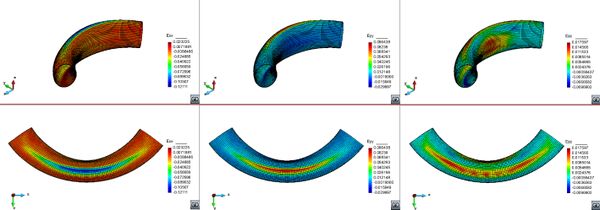
The present work aims at advancing an innovative computational methodology that simulates steel and composite material fracture under cyclic loading following a phenomenological approach, with calibration from both small scale and large scale testing. This work addresses fatigue processes ranging from High Cycle to Ultra-Low-Cycle Fatigue. An assessment of the current state of the art is done for all the different fatigue types. Following, for Ultra-Low Cycle Fatigue a new constitutive law is proposed and validated with experimental results obtained on small scale samples. Industrial applications are shown for a large diameter straight pipe under monotonic loading conditions and for a bent pipe under cyclic loading. Emphasis is made on the capacity of the model to represent different failure modes depending on the loading conditions. The research regarding this part has been used in the frame of the European Project: “Ultra low cycle fatigue of steel under cyclic high-strain loading conditions” (ULCF).
Regarding High Cycle Fatigue, a classic damage model is presented in combination with an automatic load advancing strategy that saves computational time when dealing with load histories of millions of cycles. Numerical examples are shown in order to demonstrate the capabilities of the advancing strategy and a validation of the model is done on small scale samples.
A new constitutive model is presented for Low Cycle Fatigue that uses the classic plasticity and damage theories and simultaneously integrates both processes in the softening regime. The capabilities of the model are shown in numerical examples.
Finally, the High Cycle Fatigue damage model is applied to the constituents of a composite material and the structural behaviour is obtained by means of the serial/parallel rule of mixtures. Validation of the constitutive formulation is done on pultruded glass fiber reinforced polymer profiles.
Resumen
El presente trabajo propone una metodología innovadora para la modelización numérica de la rotura de materiales metálicos y compuestos sometidos a cargas cíclicas. El enfoque es fenomenológico y la formulación se calibra con resultados experimentales obtenidos en especímenes a pequeña escala y con experimentos a gran escala. Este trabajo abarca procesos de fatiga desde alto número de ciclos hasta muy bajo número de ciclos.
Una evaluación del estado del arte hasta el momento se ha llevado a cabo para los diferentes tipos de fatiga. A continuación, se propone una nueva ley constitutiva para la fatiga de muy bajo número de ciclos y se presenta la validación con resultados experimentales obtenidos en especímenes a escala pequeña. El modelo constitutivo se ha probado en dos aplicaciones industriales: una tubería de gran diámetro bajo condiciones de carga monótonas y una tubería doblada a un ángulo de 90 grados sometida a cargas cíclicas. Se ha enfatizado la capacidad del modelo de reproducir diferentes modos de rotura dependiendo de las condiciones de carga. El trabajo referente a este modelo se ha usado en el marco del proyecto europeo: “Fatiga de muy bajo número de ciclos del acero bajo grandes deformaciones cíclicas”.
Respecto a la fatiga de alto número de ciclos, se presenta un modelo clásico de daño combinado con una estrategia automatizada de avance en la carga por número de ciclos. La estrategia conduce a un ahorro en tiempo de computación cuando se aplican millones de ciclos de carga. Las capacidades y particularidades de la estrategia de avance en la carga se enseñan en una serie de ejemplos numéricos. El modelo se valida con resultados experimentales obtenidos en especímenes a pequeña escala.
Un nuevo modelo constitutivo se presenta para la fatiga de bajo número de ciclos que se basa en las teorías básicas de plasticidad y daño y que integra simultáneamente las ecuaciones de ambos procesos en el régimen de ablandamiento. Las capacidades del modelo se enseñan a través de ejemplos numéricos.
Finalmente, se estudia la aplicación del modelo de daño para fatiga de alto número de ciclos en los componentes de materiales compuestos. El comportamiento estructural del material compuesto se obtiene a través de la teoría de mezclas serie/paralelo. La formulación se valida con resultados experimentales obtenidos en perfiles de GFRP.
Acknowledgements
I would like to thank all the people that in some way have helped me to complete my PhD.
I would like to express my gratitude to my PhD advisors, Sergio Oller, Xavier Martinez and Álex Barbat, for their faith in me and for their dedication during these years. You have contributed greatly in shaping my understanding and my knowledge both at a scientific and at a personal level. I consider myself immensely fortunate to have had the opportunity to learn from you.
I would like to thank the Spanish Minisitry of Education for the FPU Grant I have received during my PhD years and the European Union for the funding given to the "Ultra low cycle fatigue under high-strain loading conditions" project. Also, my PhD advisors for giving me the opportunity to participate in this project. The knowledge generated from the project constitutes an important part of this work.
I would like to express my gratitude to CIMNE at an institutional level for all the opportunities it has offered me in attending international conferences and for participating and assisting at many high-quality lectures held in its premises. I have found here a family away from home. Thank you Kike and Miguel for always being there when I had troubles with GiD and, together with Salva and Guillermo, for all the conversations we enjoyed daily at lunch. It has been very refreshing and thought provoking to share ideas and opinions with you and together we have made many great memories.
I would like to give a special thank you to Álex, Manuel and Stefano, my office colleagues, who have made my day to day entertaining during these years. Also, Fermin and Ester, my PLCd group mates. Thank you for all the help you have given me in these last months and for all the trips and outings we enjoyed together. Because you work so well, my work was made easier and has gained a lot.
To my dear parents, thank you for the way you raised me. I owe to you the person I am today. Pentru dragii mei parinti, va multumesc pentru felul in care m-ati crescut. Va datorez ceea ce sunt astazi.
Finally, I would like to thank my husband, Miguel Ángel Celigueta. Sharing these years with you has been one of the most intense learning experiences I have ever had. Thank you for your wisdom, your patience and your love.
Pentru bunicii mei! Mi-e tare dor de voi...
Para mis abuelos! Os echo tanto de menos...
"It is not because things are difficult that we do not dare, it is because we do not dare that they are difficult"
Seneca
"Both if you think you can do it and if you don't, you are in the right"
Henry T. Ford
1 Introduction, objectives and motivation
1.1 Antecedents
The present work aims at advancing an innovative computational methodology that simulates metal and composite material fracture under cyclic loading following a phenomenological approach, with calibration from both small scale and large scale testing.
Time varying cyclic loads produce failure of structural parts for values of stress lower than those obtained in static tests. This phenomenon is called fatigue and it is defined more generally in the ASTM E1823 standard [1] as:
the process of permanent, progressive and localized structural change which occurs to a material point subjected to strains and stresses of variable amplitudes which produces cracks which lead to total failure after a certain number of cycles.
In this definition it is possible to include all fatigue ranges, from “Ultra Low Cycle Fatigue” (ULCF), to “Low Cycle Fatigue” (LCF) and “High Cycle Fatigue” (HCF). Generally it is considered that failures in the range of 106 to 108 cycles belong to the HCF range, failures below 100 cycles belong to ULCF, and failures in between these limits are atributed to LCF.
One of the main drawbacks of most of the existing formulations to characterize ULCF, LCF and HCF is that they require regular cycles to predict material failure, or they couple the effects of non-regular cycles using the Miner rule, which requires knowing the performance of the structure under regular cycles. However, this regularity often does not exist. An example of an ULCF failure due to an irregular cyclic load is found in the failure of structures subjected to seismic loads, where the frequency varies along time and each cycle may have different amplitudes.
A Continuum Damage Mechanics (CDM) based fatigue model has been previously derived at CIMNE to address low- and high-cycle fatigue [2] and the present work is based on the thermodynamic framework adopted there. Given the extensive experience of the workgroup in constitutive modelling of composite materials, the application on long fiber composite materials of the formulation developed is also studied.
1.2 Motivation
This work addresses fatigue processes ranging from high cycle to ultra-low-cycle fatigue. While high cycle fatigue (HCF) in metals is a largely documented phenomena, less is known about its ultra-low-cycle counterpart, a phenomena caused by extreme loading conditions (e.g. earthquakes, hurricanes, support settlements) characterized by large scale yielding and large deformations which lead to fracture.
The issue of fracture is dealt with in a fundamental way in this work by examining the accuracy and validity of evolving approaches to characterize extreme loading-induced fracture in steel structures. Finite element modelling is extensively used to describe the stress and strain distribution and evolution during specimen loading. An experimental program of large scale tests pertaining to the European Project Ultra low cycle fatigue of steel under cyclic high-strain loading conditions is also used to validate and demonstrate the constitutive models proposed under monotonic and cyclic loadings.
Based on an evaluation of the current state of the art, three constitutive models are proposed in this work, that derive from a common thermodynamical and mechanical base. They make use of the basic theories of damage and plasticity in order to simulate the behaviour of materials subjected to fatigue due to complex loading scenarios. The nonlinear behaviour of the materials is reflected directly in the constitutive equation without any need of additional fracture criteria. The formulations have a wide range of applicability, both for monotonic and cyclic loading.
The effect of fatigue in composites is still an open issue not yet resolved. With the increasing use of composite materials comes an increasing need to understand their behaviour and design life. Many of the nowadays composite applications encompass conditions that include repetitive loading cycles, thus demanding the ability to understand and evaluate fatigue in composite structures.Following these considerations, one of the formulations shown in this monograph is also applied to composite materials with successful results, proving that the Continuum Damage Mechanics approach can be used for these materials.
1.3 Objectives
The main objective of this work is advancing an innovative computational methodology that simulates metal and composite material fracture under cyclic loading following a phenomenological approach, with calibration from both small scale and large scale testing.
The completion of this objective has been conditioned by the fulfillment of several specific objectives that may be summarized as follows:
- Development of constitutive laws for the description of the evolution of plastic behaviour based on the observed micromechanisms and experimental testing under ULCF conditions;
- Development of constitutive laws for the description of damage evolution based on the observed micromechanisms and experimental testing under HCF conditions;
- Development of a constitutive model for the description of plasticity and damage evolution based on the observed micromechanisms and experimental testing under LCF conditions;
- Development of an automatic load-advancing strategy that reduces and optimizes the computational time of a numerical simulation.
- Development of constitutive laws for the description of damage evolution under cyclic loading in composites using the serial/parallel mixing theory.
1.4 Outline of the monograph
The document begins with a short introduction on the general topic of fatigue followed by a review of the state of the art on processes responsible for extreme loading conditions-induced fracture, and then applying the state of the art micromechanics models for explaining cyclic fracture and fatigue prediction, first for steel members, extending the question further to composite materials.
The limitations of the existing approaches are described, knowledge gaps identified and issues regarding the implementation of these approaches are critically assessed. There will be a particular emphasis placed on damage initiation and spread due to extreme cyclic loading, known as ultra-low-cycle fatigue (number of cycles to failure on the order of 102). A review of fatigue life prediction methods in composites is then also presented.
In the following chapter a constitutive model is proposed for Ultra Low Cycle Fatigue (ULCF) with two associated constitutive laws. Validation of the laws is done on small scale samples. Industrial applications are shown for a large diameter straight pipe under monotonic loading conditions and for a bent pipe under cyclic loading. Emphasis is made on the capacity of the model to represent different failure modes depending on the loading conditions.
Regarding High Cycle Fatigue (HCF), in chapter 4 a classic damage model is presented in combination with an automatic load advancing strategy that saves computational time when dealing with load histories of millions of cycles. Numerical examples are shown in order to demonstrate the capabilities of the advancing strategy and a validation of the model is done on small scale samples.
The following chapter refers to a plastic damage model valid for Low Cycle Fatigue (LCF) that uses the classic plasticity and damage theories and simultaneously integrates both processes in the softening regime. An energy distribution law between plasticity and damage is also proposed in the softening regime. The capabilities of the model are shown in numerical examples.
In chapter 6, the High Cycle Fatigue damage model is applied to the constituents of a composite material and the structural behaviour is obtained by means of the serial/parallel rule of mixtures. This formulation is based on the composition of the fatigue behaviour of each component. Validation of the constitutive formulation is done on pultruded glass fiber reinforced polymer profiles. Special emphasis is made on the comparison between the experimental and the numerical failure mode.
The final chapter refers to conclusions that can be drawn from the work presented and future work to be done in this research line. The publications derived from the monograph are also shown and the innovative contributions of this work are emphasized.
2 State of the art
Fatigue is known to be the main cause of failure on structural parts and elements in the aeronautics, naval and automotive industry as well as in some civil engineering structures.
Steel fatigue has been extensively studied at microstructural level with a clear emphasis on its chemical and physical structure and on the influence that the latter has on material behaviour and its failure. When looking at the phenomenon from the microscale, it can be seen that a large amount of the material internal energy is spent in a rearrangement of its internal structure to accommodate better the cyclical load, followed by the gliding of the interatomic planes phase. Metal grains suffer plastic slip and non-linear behaviour [3], and these irreversible processes are responsible for crack initiation under cyclic loading.A phenomenological extension of this behaviour can be applied to composites, at each of the composite components or at their interface.
The mechanical phenomenon known as fatigue consists in the loss of material strength, and consequent failure, due to the effect of cyclic loads. Fatigue is characterized, among other parameters, by the number of cycles, load amplitude and reversion index [2]. Material failure is produced by an inelastic behaviour, micro-cracking and crack coalescence, which lead to the final collapse of structural parts.
While there is a general agreement that for failures in the range of 106 to 108 cycles the structure has failed in the High Cycle Fatigue range, there is not such agreement in defining the limits for LCF and ULCF. Authors such as Kanvinde and Deierlein [4] consider that LCF is found between 100 and 1000 cycles and that ULCF is in the range of 10 to 20 cycles; and other authors, such as Xue [5], put these limits in 104 for LCF and 100 for ULCF. However, despite these discrepancies, there is a general agreement that plastic behavior of the material plays an important role in the failure due to LCF or ULCF [6].
2.1 Methods used for the simulation of failure in steel structures
2.1.1 Strain-based design method
Given that ULCF is defined by cyclic loads which generate plastic effects, stress based design criteria for structures which are subjected to extreme loads do not yield good results. Therefore, advanced analysis and modelling of structures or components subjected to extreme loads is presently done using strain-based design criteria which are based on limit state design and displacement control load, in the sense that there are a specific subset of limit states where displacement controlled loads dominate the mechanical response of the structure.
Under the strain-based design framework, safety is established based on the variability associated with the strain demand given by design requirements on one hand, and strain capacity (which is intrinsic to the structural steel) on the other hand. To be specific, a limit state condition can be expressed as follows [7]:
- factored (increased) maximum tensile strain demand less than equal to the factored (reduced) tensile strain capacity
- factored (increased) maximum compressive strain demand is less than equal to the (reduced) compressive strain capacity
The primary areas where strain based design is expected to be applicable, taking into account the current industrial application focus of the monograph, pipelines, are in design of reeled laying of offshore pipelines, in thermal design of arctic pipelines, in design of types of offshore pipe lay systems, in design and assessment of pipelines in areas with significant expected ground movement, and in HT/HP pipeline designs. Some pipelines may also have some applications of strain-based design where cyclic loadings cause occasional peak stresses above the pipe yield strength. Here, the cyclic lifetime assessment is improved by using strain ranges for the cycles, instead of stress ranges. However, the cyclic lifetime assessment needs further development and validation, mainly for LCF or ULCF load conditions.
Some important drawbacks can be pointed out to the current state-of-the-art strain-based design [8]:
- The current use of strain-based design has many project-specific components. This limits the ability of a “cookbook” approach where each step can be laid out as part of common design sequence to apply to all areas of pipe strain-based design. This situation would indicate that taking the current state-of-the-art methods and creating a code or standard would be ineffective at covering the range of needs for future pipeline designs.
- Past design practices have asked designers to determine whether a particular loading was load-controlled or displacement-controlled without any other possible choices. Designers today need to recognize that there are a range of intermediate cases between full-load control and full displacement control. The behaviour of the pipe, particularly its buckling resistance, can change significantly depending upon the designer’s choice of the appropriate intermediate case for design. Guidance on local buckling compression resistance of pipelines appears to be well founded when using the critical strain. The additional strains that can be achieved under partly or fully displacement controlled loading should be more thoroughly studied to allow more specific guidance.
- The methods for assessing tensile failure resistance of pipelines by Engineering Critical Analysis (ECA) become fewer when the plastic strain exceeds 0.5% and fewer still as the strain increases to 2% or more. More validations trials are needed in the open literature to support the use of the few existing methods up to high axial strains.
- Further study is needed on the effects of prior strain history on the resistance of pipeline materials to different failure modes.
- Methods of assessing cycles of loading that include plastic strain are available. But the limited number of tests on which they are based may mean that these methods are conservative for many pipeline design situations to which they might be applied. Additional testing and analysis of cyclic behaviour of pipelines is needed to improve the methods currently available.
- Design of pipelines to resist ratcheting has become more important recently because of thermal cycle effects on high-temperature pipelines and flow lines. As for other types of cyclic loading, the current design methods are relatively conservative, but have been shifting to allow more cycles of plastic strain. Additional testing and assessment is needed in this area to improve the current methods.
- Although some workable strain-based design methodology and the supporting engineering processes and models have been achieved and validated, some improvements and enhancements are needed, especially as we move to high pressure, high strength pipe and large-diameter pipelines [9].
Under cyclic action, the initial loss of strength can be produced by plastic behaviour (or other non-linear phenomena) coupled with the loss of strength by fatigue, which also conduces to the high reduction of the residual strength, causing a decrease of the residual life under very low number of cycles. The capturing of this life reduction is possible by means of a new constitutive model based on the residual strength of the solids under fatigue loads coupled with other nonlinear models (ex: plasticity, ductile damage).
Plastic design is applied in two areas: for structures subjected to static loads and for structures subjected to loads varying with time. Extreme transient loading conditions involving widespread yielding may lead to monotonic ductile fractures or to fatigue failures after a very short number of load fluctuations (Nf in the order of 102 cycles). The latter failure mechanism is often called ULCF to distinguish it from the well-known low-cycle fatigue process (Nf in the order of 103 cycles or greater) since it involves distinct micromechanisms, not fully understood and characterized until now.
2.1.2 Elastoplastic fracture mechanics and Engineering Critical Analysis methods
Conventional elastoplastic fracture mechanics (EPFM), using parameters such as the J-Integral (also refered to as the Rice integral) or the Crack Opening Displacement, has been very often applied to assess the ultimate failure loads under plastic conditions. EPFM is the theory of ductile fracture, usually characterized by stable crack growth in the case of ductile metals. The fracture process is accompanied by the formation of a large plastic zone at the crack tip and material failure is determined by an energy criteria in conjunction with a yield criteria. However, this approach shows very important limitations, namely:
- it requires the assumption of an initial flaw (cannot handle flaw-free details);
- EPFM assumes small-scale (limited) yielding;
- EPFM based approaches do not explicitly include effects of reversed cyclic loading, thus cannot be conveniently applied to situations of ULCF.
Engineering Critical Analysis (ECA) is primarily used in strain-based design to set the allowable flaw size for inspection or to check that the material toughness is sufficient for a given flaw size. The methods are applied to both girth- and seam-welded areas based on the engineering understanding of brittle and ductile fracture and plastic collapse. ECA for strain-based design must use a rather high level of complexity. The assessment of flaws in areas of general plasticity was not the original domain of any of the standard assessment techniques and these have been extended to cover it by various modifications.
Damage mechanics is frequently proposed as an alternative approach to EPFM to assess the macroscopic crack initiation. This work proposes developments of the Continuum Damage Mechanics (CDM) based approach to predict the ULCF under conditions of generalized plasticity.
2.2 ULCF and LCF models
2.2.1 Coffin Manson law2.2.1 Coffin
−
{\displaystyle -}
Manson law
According to the literature review made by Yao and Munse in [10], first attempts to characterize LCF and ULCF can be attributed to Kommers who, in 1912, conducted several tests on a cantilever specimen subjected to cyclic bending. After these tests he reached the conclusion that the magnitude of deflection plays an important role in low cycle fatigue. However, main efforts to characterize the parameters driving LCF and ULCF are not found until 1950s, when numerous experimental programs where carried out to calibrate the material constants for various metals. A large amount of work is documented from this period. The experimental data is usually plotted on a log log scale with the abscissa representing the number of life cycles and the ordinate the plastic strain amplitude. This graph is known as the curve. Following this approach, probably the most known, and most widely used, procedure to predict material failure under LCF and ULCF is the Coffin Manson law [6], [11] and [12]:
|
|
(1) |
being the plastic strain range in the material, the number of cycles that can be applied before ULCF and LCF failure, and and material constants.
From this first equation proposed by Coffin and Manson, several authors have provided their own law in order to improve the accuracy on the predicted cycles before failure, especially in the ULCF regime. For instance, Xue [5] observed, from experimental results, that the law did not fit well in the range of very low life cycles, less than 100, so he proposed a new exponential damage rule that improved this accuracy. Kuroda [12] also provided a modification on the original Coffin Manson law in order to predict the failure below 100 cycles. In this case the model is based on the accumulation of damage due to three different effects: tensile straining, cyclic straining and crack propagation.
The approach used by Tateishi et al. [13] to simulate LCF failure is also interesting. These authors use Miner’s rule to couple the effect of High Cycle Fatigue with the effect of Low Cycle Fatigue, by adding a ductile damage term. This last term depends on the yield strain of the material, the rupture strain and the strain that is applied in a given cycle.
Current ULCF and LCF models may be broadly organized into two categories: those that couple the fracture behaviour with constitutive behaviour and those that do not. In the former, the effects of material damage are considered through the constitutive model while in the latter, material damage is an independent variable whose value has no direct effect on the constitutive model. Rather, the material damage combined with a fracture condition can predict geometric changes (i.e., material separation) which, in turn, will affect the constitutive response.
Since the constitutive response of coupled models is explicitly tied to the damage/fracture model, coupled models can readily predict crack propagation rate and direction, whereas uncoupled models must implement a separate material separation criterion which often pre-determines the crack path. Despite this advantage, coupled models are generally more difficult to calibrate because of additional parameters which may have loose physical meaning. Micromechanical-based models have been given a major emphasis to predict ULCF fracture. Among these models, the more relevant ones are:
- the Cyclic Void Growth Model (CVGM) proposed by Kanvinde and Deierlein [3];
- the Effective Damage Concept (EDC) developed by Ohata and Toyoda [14];
- the Leblond Model (usually called LPD model) [15] and
- the Continuum Damage Mechanics model proposed by Bonora [16].
While the first two models are uncoupled models, the latter two consider coupling between damage and constitutive equations.
2.2.2 Cyclic Void Growth Model (CVGM)
Because the mechanism of ULCF is controlled by void growth and coalescence, the CVGM proposed by Kanvinde and Deierlein [4], [3] and [17] extends upon the widely used void growth model (VGM), developed by Rice and Tracey [18], Hancock and Mackenzie [19] and others for monotonic loading. The CVGM is defined by two equations defining the fracture demands, imposed on a material by ULCF loads, and the fracture toughness of a material, under ULCF loads. The fracture condition (crack initiation) occurs when the fracture demand exceeds the fracture toughness.
In order to account for the effects of void growth and coalescence that drive the fracture of metallic materials, the authors propose a model that calculates the void growth and compares it with a critical value to detect material failure. This parameter is obtained experimentally. The initial formulation developed for monotonic cases (Void Growth Model – VGM [17]) is extended to cyclic loads by differentiating the void growth obtained in the tensile and compressive regions of the load cycle. Therefore, the void growth in the Cyclic Void Growth Model (CVGM) can be obtained as [3]:
|
|
(2) |
Two assumptions are inherent to the fracture demands:
- Voids grow during tensile cycles, where tensile cycles are defined to occur whenever triaxiality is positive;
- Voids shrink during compressive cycles, similarly defined as whenever the triaxiality is negative. In the VGM, the critical void size varies only with material; however with the CVGM the critical void size varies both with material and with the extent of material damage, induced by the reversed plasticity of the cyclic loading.
2.2.3 Effective Damage Concept (EDC)
The Effective Damage Concept (EDC), like the CVGM, is valid for arbitrary ULCF loading and controlled by the growth and coalescence of voids. The CVGM and EDC are conceptually similar. Both are based on the mechanism of void growth and coalescence with accompanying material damage induced by reversed plasticity and both are based on extensions of the VGM. Despite these similarities, there are several important differences. The EDC explicitly depends on the back stress, a second order tensor that defines the center of a material’s yield surface in multiaxial stress space. The back stress quantifies the kinematic hardening of a material. The key assumption of the EDC is that material damage accumulates only when the back stress exceeds the maximum value obtained during prior load cycles.
In implementation, the EDC is summarized by two concepts:
- Applied equivalent plastic strain, during which the back stress does not exceed the previous maximum back stress, does not contribute to material damage. Rather, only the “effective” equivalent plastic strain, contributes to material damage. The “effective” equivalent plastic strain, for a given load cycle, is defined as the portion of the total equivalent plastic strain for which the back stress equals or exceeds all prior values;
- The initiation of ductile fracture occurs when an instantaneous combination of “effective” equivalent plastic strain and triaxiality equals the failure curve.
2.2.4 The Leblond model
The formulation of the Leblond model extends upon the GNT porous metal constitutive model. The proposed modification replaces the Cauchy stress tensor, in the equation of the yield surface, with the difference between the Cauchy stress tensor and the back stress tensor and, thus, accounts for the kinematic hardening associated with cyclic loads. The proposed modification advanced by Leblond allows the prediction of the constitutive response and point of ductile fracture initiation under ULCF loads. Ductile fracture initiation occurs when the void volume fraction exceeds a material dependent critical value and the load-carrying capacity of the material reduces to zero.
2.2.5 The Pirondi and Bonora model
Pirondi and Bonora [16], inspired on works of Lemaitre [20] and Chaboche [21] proposed a CDM model in which the constitutive behaviour under ULCF is coupled with the damage state.
The main features of the CDM model are:
- Material damage is a non-linear function of the equivalent plastic strain;
- The modulus of the elasticity depends on the damage, where increases in the material damage result in decreases in the modulus of elasticity;
- Damage accumulates and its effects are active only when the mean stress is positive (i.e., the elastic stiffness is reduced only when the mean stress is positive). As such, any equivalent plastic strain that is accumulated when the mean stress is negative does not contribute to the damage nor does it alter the constitutive equations. Ductile fracture initiation is predicted when the material loses its load-carrying capacity.
2.2.6 The EVICD model
An interesting approach to characterize low cycle fatigue accounting for non-regular cycles is the one proposed by Jiang et al.[22], which defines an independent continuous cumulative damage function (EVICD) based on the accumulation of plastic strain energy. This formulation is based on the previous models of EVICD [22],[23] and [24] and states that the total damage can be computed as:
|
|
(3) |
Being the fatigue damage, the plastic strain energy density and a function determined experimentally based on the fatigue response of the material. With this approach the authors obtain an evolution of the fatigue damage parameter as the simulation evolves and the material failure is obtained when . In [22], the model is tested for fatigue ranges between 10 to 10 cycles, which corresponds to low and high cycle fatigue.
This formulation, as well as the formulation proposed by Kanvinde and Deierlein [3], are capable to account for regular and non-regular cycles, as both formulations are based on the addition of certain quantities while the material increases its plastic strain. However, they both have the drawback of being based on a failure criterion that is completely independent of the plastic model (uncoupled approaches): it is calculated as the simulation advances and, when it reaches a certain level, the criterion tells the code that the material has failed.
The simulation of LCF and ULCF has also been approached using non-linear constitutive laws. This is the case of Saanouni and Abdul-Latif [25] and [26], who propose the use of a representative volume element (RVE), and a non-linear law based on the slip theory, to account for the dislocation movement of metallic grains. Instead of a RVE, Naderi et al. [27] proposed simulating the progressive failure of a given structural element by applying random properties to the different finite elements in which it is discretized. The constitutive model used to characterize LCF failure is the one defined by Lemaitre and Chaboche in [28]. The use of a stochastic approach is also the approach used by Warhadpande et al. [29], who applied random properties to a Voronoi cell. In most of these models the damage variable is also calculated independently of the non-linear constitutive law used to simulate the material performance.
2.3 HCF models
Regarding the high cycle fatigue (HCF) phenomenon, it is known that the type of fracture involved at macroscale level occurs with little or no plastic deformation. Therefore, HCF does not introduce macroscopic plastic strain, but it introduces porosity [30]. These are the reasons that have led to describe this failure mode by means of damage models. These can be categorized into five groups: damage curve approach, crack growth- based approach, life curve modification approach, energy based damage theories and continuum damage mechanics (CDM) approaches [31]. However, in spite of the great number of models proposed in the HCF field, there is not yet a universally accepted one.
In particular, the CDM approach is based on the original concepts of Kachanov [32], [33] for treating creep damage problems. The posterior work of Chaboche [34], [35], Chaboche and Lemaitre [36], [28], Wang [37], Wang and Lou [38], Li et al. [39] and Oller et al. [2] established the CDM framework as a valid alternative to the fracture mechanics formulations in order to assess in a unified way both crack initiation and propagation. Furthermore, they enhanced the study of fatigue problems by recognizing that the theoretical structure of continuum mechanics, such as damage, is suitable for the study of nonlinear fatigue problems and that the mechanical effect known as fatigue produces a loss of material strength as a function of the number of cycles, load amplitude, reversion index, etc.
Regarding fatigue life prediction, many different approaches have been proposed such as the early methods of stress-life approach and strain-life approach [40]. One of the most used models is based on the Palmgren-Miner linear damage law [41], [42]. However, such models do not recognize the effects of prior history of loading, or the load sequence on the subsequent life. Strain-life models, on the other hand, account for the local plasticity effects at stress concentrations regions [43]. Information is abundant in literature as there are many different crack initiation models [44], with a large number of empirical models proposed for the long crack growth prediction [45]. Despite the abundant information existent on fatigue constitutive models, no attention is given to load advancing strategies utilized in numerical simulations, where one of the objectives of this work resides.
2.3.1 Continuum Damage Mechanics method
The CDM is an alternative to the Fracture Mechanics Approach, with important advantages, namely that it handles, in a unified way, both crack initiation and crack propagation.
Failure in metals and alloys is a multiscale phenomenon, in general. Macroscopic rupture is the result of the irreversible processes that occur at smaller material length-scales. Both pre-existing and load generated micro/mesoscale flaws may grow reducing the nominal material resistance. Consequently, the conditions under which failure can occur should be evaluated based on meso/micromechanics considerations. In metals, all failure modes can be ascribed only to five micro-mechanisms and their combinations: cleavage, ductile fracture, creep, fatigue, and corrosion. For all of them, the reduction of the material load carrying capability is always associated to the appearance of irreversible strain, which may be either highly localized in the microstructure, as for cleavage, or spread across the entire geometry volume, as for ductile rupture or creep.
In addition to global theories, such as fracture mechanics concepts, in the last two decades, micromechanical modelling has been proved to be a powerful approach to understand and predict failure in materials. The real advantage of micromechanics relies on the assumption that the model parameters are only material characteristics and do not depend on the geometry. Damage resulting from plastic deformation is mainly due to the formation of micro voids which initiate either as a result of fracturing or debonding from the ductile matrix, of inclusions such as carbides and sulphides. In pure metals, micro voids are nucleated at the grain triple points and along the grain boundary as a result of the incapacity of the microstructure to accommodate, in a congruent manner, the imposed displacement field. The growth of micro voids, under increasing strain level, progressively reduces the material capability to carry loads up to complete failure. A proper modelling of this micro mechanism at the mesoscale is the basis for the prediction of ductile failure in real life components and structures (i.e., the macroscale).
Damage models can be grouped in three main categories:
- Abrupt failure criteria
- Porous solid plasticity
- Continuum damage mechanics (CDM).
In abrupt failure criteria, failure is predicted to occur when one external variable, that is uncoupled from other internal variables, reaches its critical value (e.g. Rice and Tracy critical cavity growth criterion).
In porous solid plasticity, the effect of ductile damage (Gurson [46], Needleman and Tvergaard [47], hereafter GTN) is accounted for in the yield condition by a porosity term that progressively shrinks the yield surface. The GTN model, although extensively used is known to suffer from a number of limitations:
- A large number of material parameters which makes difficult to evaluate possible mutual influence;
- The material parameters are not physically based and cannot be directly measured for a material;
- A poor geometry transferability of damage parameters which often requires a posteriori adjustments;
- Damage softening introduces a length scale dependency, (mesh effect) [48].
In the last category, damage is assumed to be one of the internal constitutive variables that accounts for the effects on the material constitutive response induced by the irreversible processes that occurs in the material microstructure.
Starting from the early work of Kachanov [33], the CDM framework for ductile damage was later developed by Lemaitre [20] and Chaboche [21]. In the last two decades, a number of CDM based formulations have been proposed. Also, these models show a number of limitations:
- The proposed choice for the damage dissipation potential is, in many cases, specific of the particular material;
- Damage evolution laws are often validated only with experimental data obtained under uniaxial stress. Therefore, the transferability of parameters to multiaxial stresses is not always demonstrated;
- Similarly to the porosity models, also the CDM formulations are affected by mesh size effect due to damage softening.
More recently CDM formulations have been proposed [49] which try to overcome the above limitations: the damage variable is uncoupled from plasticity, so avoiding mesh size influence, and the damage evolution law take into account for nonlinear accumulation effects. All the cited approaches are based on the void growth and coalescence descriptions which, as already stated, strongly depend on stress triaxiality. Anyway, in the final phase of the fracture process two different mechanisms may compete, the internal necking of ligaments between voids, which is mainly influenced by medium-high values of the stress triaxiality, and the shear failure which is evident at low stress triaxiality, as described by Bao and Wierzbicki [50].
Experimental evidences of a different fracture behaviour at similar triaxiality level, but obtained from different geometrical conditions were early found by Clausing [51]. McClintock [52] also found that for many materials the equivalent plastic strain at failure is lower in torsion than in tension, even if the stress triaxiality in torsion is zero, which is not consistent with any of the hydrostatic pressure dependence (i.e. triaxiality) models described. A step forward with respect to the classical damage theories was proposed by Wierzbicki et al. [53] by introducing another normalized parameter - the deviatoric parameter, based on the third invariant of the stress tensor, beside the stress triaxiality, to capture the strain to fracture dependence from the stress state, thus covering both the hydrostatic and the shear type failure modes. The sensitivity of a material to the third invariant has as consequence the non-uniqueness of the relation between triaxiality and fracture strain, which is bound between two distinct limits (upper and lower). These evidences have also been confirmed in recent works by Barsoum [54] and Coppola [55].
In contrast to monotonic ductile failures and low/high-cycle fatigue, models are less well developed for ULCF. The fundamental physical processes responsible for this type of fracture cannot be modelled using traditional fracture mechanics and fatigue models. ULCF is often accompanied by large-scale yielding, which may invalidate stress intensity-based K- or J-type approaches. It is well known that Coffin-Manson approach used in Low-cycle fatigue tends to over-predict the cyclic life under extremely low cycle fatigue conditions [5]. Like monotonic ductile fracture, ULCF is ultimately controlled by the growth and coalescence of microscopic voids. However, the reversed plasticity induced by the severe cyclic loading degrades the fracture resistance, or toughness, due to the accumulation of material damage.
This degradation mechanism is similar, in concept, to that of low cycle fatigue. Thus, ULCF is more accurately conceptualized as an interaction between ductile fracture and fatigue.
2.4 Fatigue in composite materials
The need to apply continuum damage mechanics (CDM) based models to composite materials has been widely recognized. Efforts to conduct fatigue analysis of large structures have been hindered by excess computational time and the inability to separate differences in constitutive behaviour exhibited by each constituent of the composite. Historically, only micromechanical models have been able to treat the constituent separately. Thus, handling component material failure at a large-scale structural level was nearly impossible.
In general, the lack of understanding regarding composite structural fatigue is a significant setback for many industries. Fatigue failures represent the greatest uncertainty with regard to the long term service lifetime of the major structural components of a wind turbine [56].
One of the failure modes that is addressed in this monograph is the life prediction of composites when they are subjected to cyclic loads. The effect of fatigue in composites is a controverted issue due to the fact that fatigue is a concept associated to the crystalline structure. From a phenomenological point of view, if we understand fatigue as damage accumulation due to an increase in the number of loading cycles, the concept can be extended to composite materials. However, the loss of strength that is typically caused by fatigue cannot be so easily addressed when dealing with composites.
There are three commonly used approaches when assessing life duration for a composite material [57]:
- Strength reduction models
- Stiffness reduction models
- Effective damage models
Assuming that the strains and stresses at constituent level can be determined either by a micromodel or by simplifying theories (among which mixing theory can be considered), strength reduction models require a large number of experimental failure tests. Even so they are traditionally the most commonly used methods [57].
Stiffness reduction models have the advantage that, although a large number of experimental data is still needed, the testing can be done without fracturing the samples.
Effective damage models have been explained previously when assessing the problematic for metals. They are developed starting from the early work of Kachanov [33] under the CDM framework for ductile damage.
In a composite material, fatigue damage can take the form of any or all of the following: delamination, matrix cracking, matrix crazing, fiber/matrix debonding and void growth [57].
There are numerous studies, most of them experimental, that address this problem showing that the life prediction varies depending on the composite constituents (there is a difference between using glass or carbon fibers [58]); as well as it also varies depending on the composite configuration, such as fiber orientation [58], or in case of ply-drops [59]. This variability proves that the life prediction of composites subjected to cyclic loads cannot be addressed just with an S/N curve but it requires a detailed simulation capable to take into account all dependencies.
To meet the needs of composite structural evaluation, an effective solution to accurately model composite fatigue should [60]:
- Consider fatigue damage to a particular constituent material within the composite, not damage to the homogenized composite.
- Require a minimal input data set for characterization of fatigue behaviour.
- Apply to multiple types of loading and load histories.
- Apply to any composite laminate layup.
Early studies in predicting composite fatigue [61] relied on macroscopic composite strengths. This approach requires a minimal data set, but satisfies none of the other requirements.
Microstructural modeling of a composite can yield high-fidelity constituent stresses and strains but is too computationally intensive for large-scale structural analyses. The different micromechanical damage modes that appear in composites after fatigue loading are considered in this approach. A first but practically unrealistic attempt considering dominant crack propagation has been presented by Halpin [62]. Reifsnider [63], [64], [65], [66] and [67] developed a model based on critical and subcritical elements in the laminate, investigated by researchers like Song and Otani [68], trying to correlate critical strengths of the composite with various microdamage mechanisms, while the Charewicz and Daniel [69] approach in predicting residual strength uses an unidentified damage function. An interesting experimental study suggesting a possible correlation of damage mechanisms with load sequence effects and their impact on lifetime prediction was presented by Gamstedt and Sjögren [70].
The microstructural models claim to offer a long-term promise; to be applicable to a wide variety of materials, lay-ups and loadings with a minimal amount of experimentally obtained input. At present however, they are either in their infancy or have been applied to simple fatigue loading or else include micromechanical parameters which are difficult to obtain in structural engineering reality [71].
More complex macroscopic approaches, such as calculating residual strength or residual stiffness, have also been used, with the drawback that they require much more experimental data and still apply only to a particular laminate. The results suggest that some of the models are able to describe in several cases the phenomenon of strength degradation, while others fail to provide consistently a good prediction of this behaviour, i.e. for the various tested life fractions of the coupons under different loading conditions and for all the laminate cases studied.
For instance, the linear strength degradation model of Broutman and Sahu [72], modified to account for material non-linear degradation behaviour by introducing an additional parameter as shown in [71] and the deterministic model by Harris and coworkers [73], also enhanced with statistical features models, in most cases predict satisfactorily the residual strength of the materials considered. However, they require a considerable experimental effort for implementation and do not consistently produce safe predictions. From the point of view of the designer, the approach of the linear model of Broutman and Sahu [72] appears as a strong candidate for either glass/epoxy or carbon/epoxy laminates, at least when tensile fatigue is considered.
It is important to note that it seems that no residual strength model can be safely used universally. This is mainly due to the large scatter of the residual strength data and the simultaneous initiation and propagation of several damage mechanisms in the composite under fatigue loading.
Moreover, nearly all of these techniques require a large amount of experimental data to characterize the material. Most predictive theories pertain to a specific load history at a specific temperature and are not easily generalized to capture multiaxial load states or variable amplitude loading. In addition, any general solution must be able to be implemented into finite element codes, with computational efficiency.
The chosen approach for the present work is a strength reduction model at constituent constitutive level based on the formulation adopted for metals under cyclic loading condition. The stresses and strains of the composite constituents are calculated using the serial/parallel mixing theory (SP RoM) [74], which allows different constitutive behaviour for each of the composite components and can accurately model delamination effects which are expected to be a consequence of fatigue damage. This work fits in a research line previously explored by Mayugo in [75] where a methodology for the analysis of the fatigue degradation in composite laminates is presented. The basis for the stepwise load advancing strategy is also set there, as well as the use of a strength reduction function and generalized curves, even though the expressions of the aforementioned functions are different from the ones used in this work.
2.5 Necessity of the present approach
Based on the advantages of CDM models exposed previously and on the previous experience in the work group (a CDM based fatigue model was derived at CIMNE to address low- and high-cycle fatigue [2]) this constitutive formulation has been chosen as the base of the developments shown in this monograph. This decision has been made recognizing that the theoretical structure of continuum mechanics, such as plasticity and damage is suitable for the study of nonlinear fatigue problems and that the mechanical effect known as fatigue produces a loss of material strength as a function of the number of cycles, reversion index, load amplitude, etc. This loss of strength induces the material to inelastic behaviour, which may be interpreted as micro-cracking followed by crack coalescence, leading to the final collapse of structural parts. Particularly, the proposed constitutive models establish the relationship between this residual strength and the yield surface, controlled by the standard internal variables plus a new internal variable of fatigue that incorporates the influence of the cyclic loads.
3 Constitutive modelling of Ultra Low Cycle Fatigue
3.1 Introduction
ULCF can occur in the metallic materials of modern steel devices that are designed to absorb seismic energy by sustaining large inelastic deformations under cyclic loads. Also, pipelines installed in seismic or permafrost regions must have sufficient strength against buckling or fracture caused by large ground deformation.
ULCF can be defined as a failure that occurs at a relatively small number on the repeated stress or strain cycles. The upper limit in ultra low cycle life has generally been selected arbitrarily by different researchers to lie in the range of 10 to 10 cycles. On the other hand, the lower limit of life is the static test which has been represented by various investigators as 1/4, 1/2, 3/4 or even one cycle ([10], [76]). For ductile metals under periodic plastic loading, materials often fail within a reduced number of life cycles. Within this regime, the failure mechanism is governed by the plastic and damage (or sometimes called ductile damage), which is characterized by micro structure deterioration such as micro void nucleation, growth and coalescence and micro crack initiation and propagation [5]. So, this process is governed by void growth and coalescence-type mechanisms, which are associated, typically, with ductile fracture phenomenon driven by Bauschinger plasticity non-linear mechanical processes, depending of the plastic strain [77].
While previous studies (e.g., Kuwamura and K. Yamamoto [78]) have identified this issue, models and mechanisms to characterize ULCF are not well established. Prediction models for the cyclic life of materials are thus often based on the alternating plastic and damage strain amplitude. The most commonly used relationship between the alternating damage and plastic strain and the life cycles is the so-called uniaxial Manson–Coffin law ([76], [79]), based on small uniaxial strains formulation. This law is essentially a two parameter power law curve and can be plotted in a log–log scale as a straight line where the slope of the curve depicts the exponent of the power law relationship.
The ULCF mechanical processes cannot be modelled using traditional fracture mechanics and fatigue models. Primarily, ULCF is often accompanied by large inelastic strain (damage and/or plasticity), which may invalidate stress intensity-based or approaches [80]. Second, the induced loading histories are extremely random with very few cycles, making them difficult to adapt to conventional cycle counting techniques such as rain flow analysis ([42], [81]) or strain life approaches. Finally, or methods, require an initial sharp crack or flaw, which is absent in many structural details. These limitations, coupled with the large strain advanced finite-element formulation methods, create the need for an improved understanding of the underlying ULCF process and the development of models to predict it.
Since 1950s, numerous experimental programs have been carried out to calibrate the material constants for different steels and a large amount of information is available . The experimental data is usually plotted on a log–log scale with the abscissa the number of life cycles and the coordinate the plastic strain amplitude, which is known as the curve. From the experimental results, it is observed that the Manson–Coffin law does not fit well in the range of very low life cycles, i.e. about less than 100 cycles [5]. ULCF damage is bounded by monotonic ductile failure and low-cycle fatigue (LCF). Typically, models for ULCF are extensions of LCF models. However, it is recognized in the literature that LCF models are not fully adequate without any kind of correction.
In this context, the use of a plastic damage model to simulate ULCF is proposed, and a new isotropic hardening law is presented. The model is the well-known Barcelona plastic damage model, proposed by Lubliner et al. [82],[83], [84] and [85]. An innovative application is given to this formulation by considering it for the cyclic loading case and incorporating a Friederick-Armstrong kinematic hardening law that allows the description of phenomena like cyclic ratcheting (under stress control conditions) or cyclic stress relaxation (under strain control or elastically constrained conditions). A new isotropic hardening law is developed especially for steel materials, designed to reproduce their hardening and softening performance under monotonic and cyclic loading conditions. The complete nonlinear constitutive model is an extension of a given plasticity model to incorporate the damage effects due to cyclic action. It is an energetic based approach that accounts for the energy dissipated during the plastic action and compares it with a fracture energy that has to be calibrated by experiments. The model considers that complete failure is obtained when all the fracture energy of the material is dissipated. A first preliminary description of the procedure used by the proposed model has been presented in [86] and the results shown in this chapter have been published in [87] and [88].
This work proves that the proposed model it capable of simulating material failure due to ULCF by its own, without the need of any other damage variable computed independently of the plastic formulation. Besides, the proposed approach is not only capable of predicting material failure for regular and non-regular cyclic loads, but it is also capable of coupling cyclic loads with monotonic loads, which allows predicting that the structure will fail sooner if the monotonic load is applied after several hysteresis cycles, than if these cycles are not applied. This capability is obtained as a consequence of the fact that the material failure is predicted by the plastic non-linear constitutive equation itself. Another advantage of the formulation proposed is that it is capable of using any yield and potential surfaces to characterize the material, which increases its applicability to different steel alloys.
In Section 3.2 an outline of the constitutive model is made and in sections 3.3 and 3.4 of this chapter the new isotropic hardening law is presented in two different versions. In Section 3.4.3 the complete calibration procedure on small scale samples is presented step by step. Section 3.5 illustrates the results made on a 16-inch 90 elbow subjected to a variable in-plane displacement and internal pressure. In Section 3.6 results are shown for a large diameter straight pipe under monotonic combined loading: uniaxial displacement and internal pressure. Two different loading histories are taken into account that exhibit different failure modes. Finally, the advantages of the constitutive model proposed are emphasized in Section 3.7.
3.2 Plastic damage model
The inelastic theory of plasticity can simulate the material behaviour beyond the elastic range, taking into account the change in the strength of the material through the movement of the yield surface, isotropic and kinematic. It is assumed that each point of the solid follows a thermo-elasto-plastic constitutive law (hardening/softening) ([82], [89] and [90]) with the stress evolution depending on the free strain variable and plastic internal variables.
3.2.1 Plastic Model
Since this work is guided to mechanical problems with small elastic strains and large inelastic strains, the free energy additivity hypothesis is accepted ([91], [92]). The elastic and plastic parts of the free energy are written, in the reference configuration for a given entropy and temperature field, as the elastic Green strains ; the two last variables operate as free field variables ([89], [92] and [93]). The free energy is thus written as,
|
|
(4) |
Considering the second thermodynamic law (Clausius-Duhem inequality, [91], [94] and [95]), the thermo mechanical dissipation can be obtained as [92]:
|
|
(5) |
The accomplishment of this dissipation condition, equation 5, demands that the expression of the stress and the entropy should be defined as (Coleman method; see [95]);
|
|
(6) |
From the last expression is possible to obtain the general expression of the tangent constitutive tensor,
|
|
(7) |
where is the material density, , , are the total, elastic and plastic strain tensors, respectively, is the stress tensor for a single material point, and are the initial and tangent constitutive tensors, and are the plastic internal variables.
3.2.2 Yield plastic functions
The yield function accounts for the residual strength of the material, which depends on the current stress state, the temperature and the plastic internal variables. This function and the plastic potential have the following form, taking into account isotropic and kinematic plastic hardening (Bauschinger effect; [28], [96] and [97]),
|
|
(8) |
where and are the uniaxial equivalent stress functions depending of the current value of the stresses , the kinematic plastic hardening internal variable, is the plastic strength threshold, is the plastic isotropic hardening internal variable, and is the temperature at current time ([82],[89] and [90]).
The evolution law for the plastic strain obtained from the evolution of the plastic potential as,
|
|
(9) |
Being the plastic consistency parameter. We will talk of associated plasticity when the plastic potential is the same as the plastic yield function.
3.2.3 Kinematic Hardening
Kinematic hardening accounts for a translation of the yield function and allows the representation of the Bauschinger effect in the case of cyclic loading. A two dimensional representation of this movement in the plane is shown in figure 1:

|
| Figure 1: Translation of the yield surface result of kinematic hardening |
This translation is driven by the kinematic hardening internal variable which, in a general case, varies proportionally to the plastic strain of the material point ([28], [98]). There are several laws that define the evolution of this parameter. Current work uses a non-linear kinematic hardening law, which can be written as:
|
|
(10) |
Where and are material constants, is the plastic strain, and is the increment of accumulative plastic strain, which can be computed as: . Note that the 2/3 is valid in case of using Von-Mises as the actual yield surface. In other cases, this value should be modified.
3.2.4 Isotropic Hardening
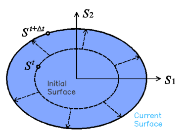
Isotropic hardening provides an expansion or a contraction of the yield surface. The expansion corresponds to hardening and the contraction to a softening behaviour. In figure 2 a two dimensional representation of this effect in the plane is depicted:
|
| Figure 2: Expansion of the yield surface result of isotropic hardening |
The evolution of isotropic hardening is controlled by the evolution of the plastic hardening function , which is often defined by an internal variable . The rate equation for these two functions may be defined, respectively:
|
|
(11) |
where denotes scalar and states for a tensor function. Depending on the functions defined to characterize these two parameters different solid performances can be obtained. Two new functions valid for characterizing metallic materials are proposed in this work and described in sections 3.3 and 3.4 of this document.
3.2.5 Stress-strain relation and consistency factor
Once the material has exceeded its yield threshold, the stress-strain relation is defined by the tangent stiffness matrix. The expression of this matrix, as well as the expression of the plastic consistency parameter can be obtained from the plastic yield criterion and the Prager consistency condition [98]:
|
|
(12) |
Using previous expressions, it is possible to rewrite equation 12 as:
|
|
(13) |
From this expression it is possible to obtain the consistency factor using equation 9.
|
|
(14) |
Therefore:
|
|
(15) |
The tangent stiffness tensor relates the total strain rate to the stress rate:
|
|
(16) |
Finally, the expression of the tangent stiffness matrix can be obtained from the consistency factor:
|
|
(17) |
It has to be noted that expression 17 has been obtained disregarding the non-linear term of kinematic hardening. Despite having a first approximation of the analytical expression that provides the tangent stiffness tensor, in many occasions the calculation of the partial derivatives of the yield and potential functions is not straightforward. In those cases, a numerical derivation can be performed. This procedure, although expensive, provides an accurate approximation that improves the global convergence of the problem. An efficient procedure to conduct this numerical derivation, as well as the advantages obtained with it, are shown in [99]. A detailed description of the integration procedure of the constitutive equations can be found in references [92] and [98].
3.3 New isotropic hardening law
Equation 11 allow the incorporation of different hardening laws to describe the material performance. In the Barcelona model defined in [82], the laws defined are driven by the fracture energy of the material. This work presents a new law, specially developed for steel materials, that has been designed to reproduce their hardening and softening performance under monotonic and cyclic loading conditions. This law also depends on the fracture energy of the material.
3.3.1 Fracture Energy
Classical fracture mechanics defines the fracture energy of a material as the energy that has to be dissipated to open a fracture in a unitary area of the material. This energy is defined as:
|
|
(18) |
where is the energy dissipated by the fracture at the end of the process, and is the area of the surface fractured. The total fracture energy dissipated, , in the fracture process can be used to define a fracture energy by unit volume, , required in a continuum mechanics formulation:
|
|
(19) |
This last equation allows establishing the relation between the fracture energy defined as a material property, , and the maximum energy per unit volume:
|
|
(20) |
Thus, the fracture energy per unit volume is obtained as the fracture energy of the material divided by the fracture length. This fracture length corresponds to the distance, perpendicular to the fracture area, in which this fracture propagates.
In a real section, this length tends to be infinitesimal. However, in a finite element simulation, in which continuum mechanics is applied to a discrete medium, this length corresponds to the smallest value in which the structure is discretized: the length represented by a gauss point.
Therefore, in order to have a finite element formulation consistent and mesh independent, it is necessary to define the hardening law in function of the fracture energy per unit volume ([82], [90], [100]). This value is obtained from the fracture energy of the material, , and the size of the finite element in which the structure is discretized.
3.3.2 Hardening Function and Hardening Internal Variable
The hardening function defines the stress of the material when it is in the non-linear range. There are many possible definitions that can be used for this function fulfilling equation 11. Among them, the use of a function that describes the evolution of an equivalent uniaxial stress state, like the one shown in figure 3, is proposed here.
This equivalent stress state shown in figure 3 has been defined to match the uniaxial stress evolution described by most metallic materials. After reaching the yield stress, the curve is divided in two different regions. The first region is defined by curve fitting from a given set of equivalent stress-equivalent strain points. The curve used to fit the points is a polynomial of any given order defined using the least squares method. The data given to define this region is expected to provide an increasing function, in order to obtain a good performance of the formulation when conducting a cyclic analysis.

|
| Figure 3: Evolution of the equivalent stress |
The second region is defined with an exponential function to simulate softening. The function starts with a null slope that becomes negative as the equivalent plastic strains increase. The exact geometry of this last region depends on the fracture energy of the material. The adjustment of this exponential softening to experimental results is usually very difficult, as the stress drop is very fast and experimental tests cannot capture it. Therefore, its definition will be done just to obtain a more or less steep slope. The selection of an exponential function instead of a straight line or a polynomial is made because the exponential function provides a response that facilitates the numerical convergence.
It has to be noted that the initial plateau that is usually found in monotonic stress-strain graphs of carbon steels is not represented in the stress evolution proposed in this model and, therefore, it is not shown in figure 3. This is because the definition of this region will lead to inaccurate results when performing cyclic simulations of the material.
The hardening internal variable, , accounts for the evolution of the plastic hardening function, . In current formulation is defined as a normalized scalar parameter that takes into account the amount of volumetric fracture energy dissipated by the material in the actual strain-stress state. This is:
|
|
(21) |
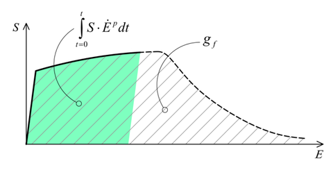
Figure 4 shows shaded in green the volumetric fracture energy required by a uniaxial material, for a given plastic strain . The hardening internal variable defined in 21 is calculated normalizing this fracture energy by the total fracture energy of the system, , which corresponds to the total area below the curve , shaded with grey lines.
|
| Figure 4: Representation of the volumetric fracture energy of a metallic material |
Using the definition of the hardening internal variable defined in equation 21, it is possible to define the expression of the hardening function as:
|
|
(22) |
It can be easily proven that the hardening function and internal variable defined in equations 21 and 22 fulfill the rate equations 11. The and functions defined in expression 11 become:
|
|
(23) |
3.3.3 Expressions of the hardening function
In this section the exact numerical expressions used to define the new hardening law presented in this work are provided. This law is characterized with two different functions, each one defining the evolution of the equivalent stress in each region in which the equivalent stress performance is divided (see figure 3).
Region 1: Curve fitting with polynomial
The first region is characterized with a polynomial defined by curve fitting from a given experimental data. Among the different available methods that can be used to define this polynomial, here the use of the least squares method is proposed due to its simplicity, computational cost, and good performance provided. The resulting relation between the stress and plastic strain in this region is:
|
|
(24) |
with the order of the polynomial.
The volume fracture energy that is dissipated in this region can be obtained calculating the area below the graph. This provides the following value:
|
|
(25) |
being and the initial and final plastic strain values, respectively, that delimit the polynomial function region.
Although the equivalent plastic stress should depend on the plastic internal variable , in a cyclic simulation with isotropic hardening this approach will produce hysteresis loops with increasing stress amplitude (for a fixed strain amplitude). For this reason, current formulation calculates the equivalent plastic stress using the value of the equivalent plastic strain, which is obtained as:
|
|
(26) |
with defined by the yield surface used to simulate the material, as it is shown in equation 8.
Finally, the derivative of the hardening function can be calculated with the following expression:
|
|
(27) |
Expression 27 is valid for values of that are comprehended between and . The value of the upper limit of the internal variable shows that it is necessary to define a value for the volumetric fracture energy of the material larger than . If the value defined is lower, the material will not be able to reach its ultimate stress as this will imply having a fracture internal variable larger than .
Region 2: Exponential softening
When the plastic internal variable reaches the volumetric plastic energy available for the first region, , exponential softening starts in region two. The function that defines this new region is defined with the following parameters:
- The initial equivalent stress value is defined by the equivalent stress reached in the first region (). This value can be the one defined in the material characterization or can be a lower value if there has been some plastic energy dissipation in a cyclic process. In this last case, the stress value has to be obtained from previous region.
- The initial slope of the function is zero.
- The volumetric fracture energy dissipated in this region is the remaining energy in the material:
|
|
With these considerations in mind, the resultant equation that relates the equivalent stress with the plastic strain is:
|
|
(28) |
where
The expression of the equivalent stress as a function of the hardening variable is obtained combining equations 28 and 21, resulting:
|
|
(29) |
being,
And the derivative of the hardening function is:
|
|
(30) |
3.3.4 Validation of the proposed formulation
In the following, the results obtained from several simulations conducted to validate the formulation previously presented are included. This validation has been done comparing the numerical results with some of the experimental results obtained in the framework of the Ultra Low Cycle Fatigue Project [101].
3.3.4.1 Description of the experimental tests
Monotonic and cyclic tests were performed in a close-loop servo-hydraulic machine, INSTRON 8801, rated to 100 kN. The tests were performed at room-temperature in air. The fatigue tests were conducted under constant strain amplitudes and with a frequency adjusted to result an average strain rate of 0.008s. The longitudinal strain was measured using a clip gauge with limit displacements of 2.5 mm with a gauge length of 12.5 mm (INSTRON 2620-602). This extensometer was also used in two monotonic tensile tests allowing the registration of the longitudinal strains until approximately 17%
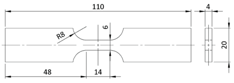
All tested specimens were machined according the longitudinal direction of 6 inch pipes made of X52 steel. The dimensions of the specimens are in accordance with the ASTM E606 standard, as illustrated in figure 5. The shown specimen corresponds to the SP series. The side faces of the specimens were milled and finished in order to remove the circumferential pipe curvature as well as surface imperfections. In order to achieve larger strain values in the specimen some of them where machined in order to reduce their section in their middle. This is the case of the OH specimen, shown in figure 6, in which the geometry is modified with an oval hole in its center. The experimental results obtained for this specimen have been also used to validate the model performance.
|
| Figure 5: Dimensions, in millimeters, of the SP specimen |

|
| Figure 6: Dimensions, in millimeters, of the OH specimen |
3.3.4.2 Description of the numerical models
Two different numerical models have been defined, one for each experimental specimen. Figure 7 shows the meshes of both models. The SP model is made with 1608 quadratic hexahedral elements and 8839 nodes. It has three elements along its thickness and 563 elements in the face shown in figure 7 (YZ). The OH model has 3080 quadratic hexahedral elements and 15460 nodes. It has five elements along the thickness and 616 elements in the YZ face. This second model requires nearly double the number of elements because the element size has to be significantly smaller around the hole for its correct simulation.

|
| Figure 7: Mesh defined for the SP and OH numerical models. The SP model has marked, with red dots, the points used to calculate the equivalent strain applied. |
Regarding boundary conditions, the left border of the model has the displacement fixed to zero in all its directions, while the right border is moved with an imposed displacement in the longitudinal direction of the sample. The reaction force is obtained as a result of the numerical analysis.
All samples analyzed are defined with the same plastic material, defined with an associated plasticity and Von-Mises as yield law. The material properties are obtained with the calibration process that is described in the following section. All the material properties required by the model are displayed in table 1. A parameter of this table that may seem surprising is the value of the yield stress, which is lower than the one expected for an X52 steel. This value is required because, if the yield stress is defined with a higher value, the kinematic hardening parameters lead to stress values too high in the hysteresis cycles. As the purpose of the model is the simulation of ULCF, which requires large plastic strain values, the requirement of defining a lower yield stress is not considered a major drawback.
| Young Modulus | 180 | GPa |
| Poisson Ratio | 0.30 | |
| Yield Stress () | 240 | MPa |
| Plastic Strain threshold () | 13 | % |
| kinematic hardening param. | 60 | GPa |
| kinematic hardening param. | 280 | |
| Fracture Energy () | 1.9 | MN * m/m |
The hardening region is defined with a polynomial of order five which is computed with the least squares method using the available experimental data. The constants of this polynomial, following the notation shown in equation 24, are shown in table 2. In order to define the polynomial constants, it has been necessary to take into account that the effects of the kinematic and the isotropic hardening laws are coupled. This implies that the definition of the first region of isotropic hardening cannot be obtained from the experimental curve straightforward, as this curve does not take into account the displacement of the yield surface due to the kinematic hardening law.
| 2.4000E+08 | |
| 8.0084E+07 | |
| -1.1143E+08 | |
| 8.7400E+07 | |
| -3.0507E+07 | |
| 3.9073E+06 |
3.3.4.3 Calibration of the numerical model
The material data previously exposed has been obtained by model calibration. This is, adjusting the different parameters required by the model to obtain a good fitting with one of the experimental results available. For the current case, the experimental results considered are those of the specimen loaded with an imposed strain range of 2.75%
The results used to conduct the material calibration are the equivalent stress-equivalent strain graphs obtained from the experimental test. The stress is computed as the total force applied to the specimen divided by the area of the cross section. The strains are computed dividing the measured displacement of the clipped gauge by the length of the gauge. In the numerical model these two parameters were calculated following the same procedure, using the red nodes depicted in figure 7.
The initial material parameters used in the calibration process are ones commonly found in literature and the polynomial constants correspond to the ones obtained by curve fitting of the experimental results, ignoring the effect of kinematic hardening. Based on the strain-stress graph obtained with these first values, the different parameters shown in table 1 and table 2 have been modified until obtaining a numerical result that fits the experimental results.
Figure 8 shows the stress-strain graph provided by the two experimental samples tested and by the numerical model, which uses the material parameters obtained from the calibration process and described in table 1 and in table 2. As it can be seen, the agreement in the cyclic behaviour of the numerical and experimental samples is rather good. This agreement is not achieved in the first loading cycle, as the model developed is not prepared to reproduce the initial plateau defined by the material. However, this disagreement is not considered relevant, as the model has been developed thinking of the cyclic behaviour and the evolution of plastic response for larger plastic strain values, found beyond this initial plateau.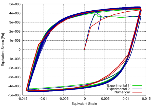
|
| Figure 8: Stress-strain graphs for the SP sample with an applied deformation range of 2.75% |

|
| Figure 9: Values of for the SP sample with an applied deformation range of 2.75%, when applying the maximum tensile and compression strain before ULCF failure. Deformation is magnified by 20. |
The mechanical performance of the numerical specimen along the simulation is shown in figure 10, where the stress-strain loops for different cycles are represented. This picture shows that the effect of material softening in the specimen consists of a reduction of the equivalent stress obtained as the number of cycles applied to the specimen increase. The figure shows that softening has already started in cycle 60, although the difference between the first loop and loop 60 is very small. In further cycles the effect of softening becomes more visible, until material failure in cycle 128, where the reduction of equivalent stress is close to a 20% Figure 10 also shows that the strain amplitude increases with the number of cycles applied to the specimen. This increase is obtained because equivalent strain is calculated as the relative displacement of two given nodes (red dots in figure 7), divided by the original length between both nodes, and does not take into account that it is modified due to the plastic deformations existing in the whole specimen.
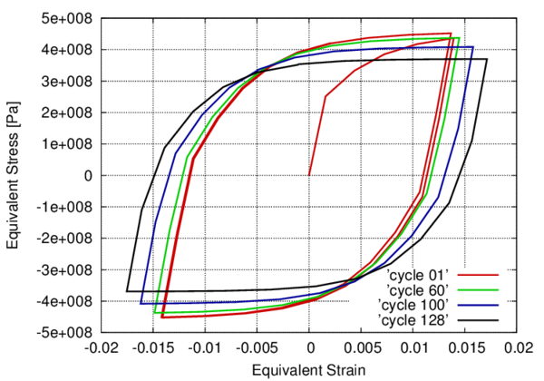
|
| Figure 10: Evolution of the stress strain graph for different cycles of the SP numerical analysis |
The results shown for the calibration test prove that the constitutive law proposed can be adjusted to any given stress-strain law by adjusting properly the material parameters. The calibration model has also been used to show the numerical and mechanical performance of the formulation developed. The prediction capacity of the model will be shown in further simulations, in which the material parameters are fixed and are used to analyze different specimens and load cases.
3.3.4.4 Validation of the developed theory
After having calibrated the material parameters, the rest of experimental tests available have been simulated in order to compare the ULCF failure prediction made by the numerical model with the results obtained from the experimental campaign. The constitutive model proposed in this work will succeed if it is capable of representing accurately the equivalent stress-strain graphs for the different deformation ranges tested experimentally and, even more important, if it is capable of predicting the number of cycles that can be applied to the specimen before its failure.
Figure 11 shows the stress-strain graph corresponding to the experimental and numerical sample with an applied equivalent strain of 4% In order to achieve this strain value, and to avoid the buckling of the specimen, the experimental test is conducted only on the positive strain region and with an antibuckling device. As can be seen, the experimental and the numerical results are in good agreement of the cyclic region of the curve. So, with this example it is proved that the model is capable of reproducing large strain values and non-symmetric cyclic patterns.
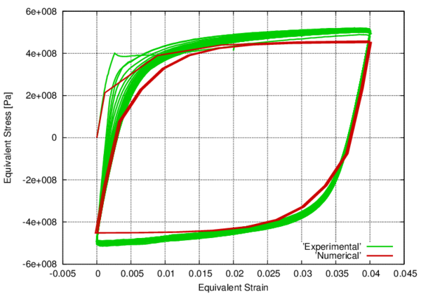
|
| Figure 11: Stress-strain graphs for the SP sample with an applied deformation range of 4.00% |
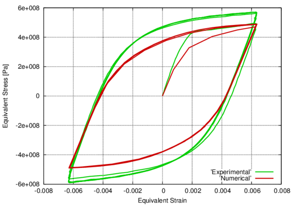
|
| Figure 12: Stress-strain graphs for the OH sample with an applied deformation range of 1.20% |
Finally, figure 12 compares the stress-strain experimental-numerical results obtained for one of the OH samples. The stress value for the OH samples is computed with the same procedure used for the SP samples, dividing the total force applied by the area of the cross section where the notch is found; and the strain value is obtained dividing with the gauge length described in section 3.3.4.1.
In this case, the numerical result prediction falls a bit shorter in terms of equivalent stress when compared to the experimental test. However, a closer look to the experimental curve shows that in the first loading branch the experimental and numerical tests match perfectly, and it is in further cycles that the experimental test provides larger equivalent stress values. This difference between cycles in the experimental test may be due to some sort of hardening around the notch, which cannot be captured by the proposed model. Despite this difference, results are considered similar enough to validate the material parameters defined in the numerical model calibration.
Once having proved that the developed formulation is capable of reproducing quite accurately the mechanical response obtained with the experimental samples, the following step is to verify if the formulation is capable of predicting the failure of the specimens due to ULCF. This validation is performed counting the number of cycles that can be applied to the numerical model before its failure. The numerical model is considered to have failed when the convergence of the analysis is lost. This occurs when some gauss points reach a value close to 1,0. The number of cycles applied to the numerical model are compared with the cycles obtained in the experimental campaign.
Figure 13 shows the results obtained for the SP samples. Results with reversion strain factor of –1 and of 0 are plotted together because the reversion factor does not play a significant role in the material response to ULCF. This figure shows that the number of cycles to failure predicted by the numerical simulation are in very good agreement with the number of cycles obtained in the experimental campaign. The only value that is not contained between the experimental results is the one corresponding to an applied strain range of 3.5% However, the value provided by the numerical simulation looks more coherent than the one obtained with the experimental test, as the number of cycles obtained in the experimental test is larger than the one obtained for an applied strain range of 2.75%
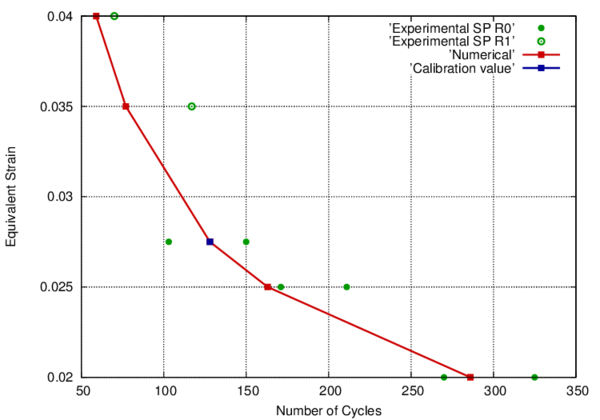
|
| Figure 13: ULCF failure prediction for SP samples |
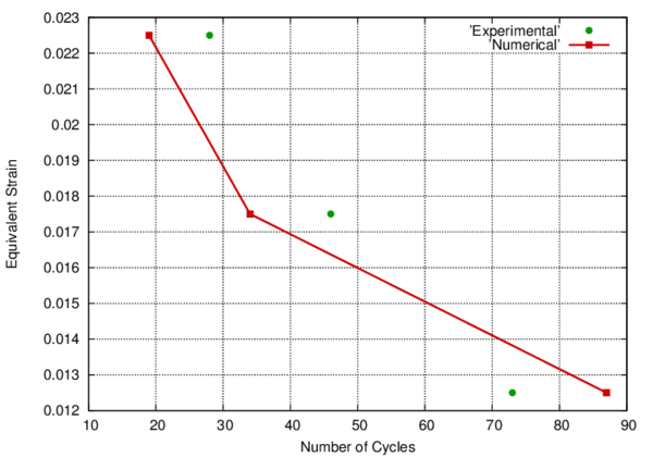
|
| Figure 14: ULCF failure prediction for OH samples |
The results obtained for the OH samples are shown in figure 14. For these samples the experimental test was conducted in just one specimen for each strain value, therefore there is no possibility to know the scatter expected in the experimental tests. However, the number of cycles predicted by the formulation is, for all strains, in the same order of magnitude than the experimental results obtained. Therefore, it can be concluded that the formulation is, again, capable of predicting accurately the ULCF failure of the OH specimens.
It is important to remark that the material properties used for all numerical simulations are exactly the same. Therefore, the variation in the prediction of the number of cycles that can be applied to any of the specimens considered is the result of the energy dissipated in each case. The agreement obtained in all cases, independently of the reversion factor or the stress concentrations due to the existing hole (OH sample) allows considering the approach used to characterize ULCF failure an excellent option. Moreover the formulation allows conducting simulations in which the cycles can be non-regular, with varying amplitude and frequency, in which there can be sustained monotonic loads between cycles or, in general, in which the load applied is not a regular one. This capability is not offered by any other formulation available.
3.4 Extension of the new isotropic hardening law for large problems
3.4.1 Hardening Function and Hardening Internal Variable
The constitutive law presented in section 3.3 has been modified in order to ensure faster convergence in the numerical model and therefore make feasible the application of the model on large problems.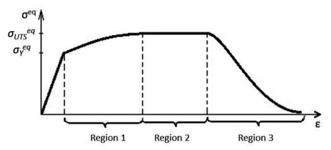
|
| Figure 15: Evolution of the equivalent plastic stress |
The equivalent stress state shown in figure 15 is different from the one presented in section 3.3 in the sense that the region obtained thru curve fitting is divided into two: a smaller region that is still dependent on curve fitting of experimental points and a linear region, with slope and extension defined by user. That helps ensure a fast integration of the stresses in the constitutive model by converging to the same numerical tolerance in less iterations. The first region is, therefore, defined by curve fitting from a given set of equivalent stress-equivalent strain points. The curve used to fit the points is a polynomial of any user given order, defined using the least squares method. The data given to define this region is expected to provide an increasing function, in order to obtain a good performance of the formulation when performing cyclic analysis.
The second region, as mentioned above, is defined as a linear curve. This region is incorporated to facilitate the convergence of the problem. If region 1 and 2 were to be simulated with just one polynomial, the difference in slope between the beginning of the curve and the end of it would make it very difficult to ensure that the slope of the polynomial is always positive so that the solution does not converge to a local minimum. Generally speaking, in the case of ULCF and LCF nearly 80% or more of the internal energy of the material is spent between regions 1 and 2.
The third region is defined with the same exponential function to simulate softening as in section 3.3. The function starts with a null slope that becomes negative as the equivalent plastic strains increase. The exact geometry of this last region depends on the fracture energy of the material (figure 16).
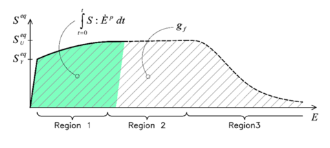
|
| Figure 16: Representation of the volumetric fracture energy of a metallic material |
3.4.2 Expressions of the hardening function
In this section, the exact numerical expressions used to define the new hardening law are discussed. This law is an evolved version of the one presented in section 3.3, as said before. The region described by curve fitting in the above reference has been divided into two different regions (Region 1 and Region 2 in figure 15). This has been done in order to optimize the constitutive law for converging to the same tolerance in fewer iterations and making feasible the large scale simulations presented in sections 3.5 and 3.6 of this chapter. The length of the curve fitting region has been limited to a user defined value and past this value of the plastic strain a linear curve has been defined with a user defined slope.
Region 1: Curve fitting with polynomial
The first region is characterized with a polynomial defined by curved fitting from a given experimental data. The exact mathematical definition for this region can be found in 3.3.3 .
Expression 27 is valid for values of that are comprehended between and .
Region 2: Linear curve
When the equivalent plastic strain, as calculated with equation 26, equals the value of equivalent plastic strain at which region 2 is to begin,, where is user defined, the threshold function is obtained taking into account the following considerations:
- The initial equivalent stress value is defined by the equivalent stress reached at the end of the first region ().
- The slope of the function is user defined: .
- The volumetric fracture energy dissipated in this region is .
With these considerations in mind, the resulting equation that relates the equivalent stress with the plastic strain is:
|
|
(31) |
The expression of the equivalent stress as a function of the hardening variable is obtained combining equation 31 and 21:
|
|
(32) |
Expression 32 is valid for values of that are comprehended between and . The value of the upper limit of the internal variable shows that it is necessary define a value for the volumetric fracture energy of the material larger than . If the value defined is lower, the material will not be able to reach its ultimate stress as this will imply having a fracture internal variable larger than .
Region 3: Exponential softening
When the plastic internal variable reaches the volumetric plastic energy available in the first two regions: . At this point, isotropic hardening is defined by region three. Its function is obtained with the following parameters:
- The initial equivalent stress value is defined by the equivalent stress reached at the end of the second region ().
- The initial slope of the function is zero.
- The volumetric fracture energy dissipated in this region is the remaining energy in the material:
With these considerations in mind, the governing equations are the same as in 3.3. The constitutive model described in Sections 3.2, 3.3 and 3.4 has been implemented in the in-house code PLCd [102]. The code was programmed to allow OpenMP parallelization, which greatly reduced the computational cost of the large scale FE simulations, and makes use of the load advancing strategy proposed in [103] and [104] and shown later on in this work in chapter 4.
3.4.3 Material calibration
The material characteristics for the numerical simulations will be obtained by conducting a calibration analysis on small scale specimens. The hardening - softening law presented in section 3.4 requires of the following material parameters:
- – points obtained from uniaxial monotonic tensile tests necessary for curve fitting. They are important for a correct representation of the tendency of the monotonic curve.
- Kinematic coefficients in accordance with the type of hardening chosen. They are important for the exact adjustment of the monotonic curve and for an accurate description of the hysteresis loop.
- Equivalent plastic deformation, , at which the linear region starts. This parameter is important both in the monotonic curve and in the overall cyclic behaviour as it ensures a stable behaviour throughout the fatigue life.
- Equivalent plastic deformation, , at which softening starts.
- Fracture energy G required in the monotonic curve for adjusting the slope of the softening behaviour and in the cyclic behaviour for correctly calibrating the fatigue life of the specimen. When the entire energy is spent the specimen is considered completely fractured.
For the industrial applications shown in this work two different materials have been calibrated, X52 and X60, for the second law, presented in 3.4. The step by step calibration process is presented for the X60 material. Another calibration process has been shown in section 3.3 for the X52 steel using the first version of the constitutive law.
In order to exemplify the calibration process, a smooth X60 specimen was chosen from the experimental program ran by Pereira et al. [101]. This experimental program includes monotonic tests and cyclic tests in the LCF and in the ULCF regime. LCF tests have been conducted both with a reversion factor of -1 and 0, while all the ULCF tests have a reversion factor equal to 0. The geometric characteristics of the specimen are shown in figure 17. This material will be posteriorly used for the large scale simulation of the bent pipe under cyclic loading shown in section 3.5.
The specimen was meshed into 3456 quadratic hexahedral elements with 20 nodes each and 27 integration points, adding to a total of 17165 mesh nodes.
The procedure for the correct calibration of the material starts from the determination of the elastic modulus and of the elastic limit. These two parameters are determined statistically from the force – displacement recordings of both the monotonic and the cyclic tests by monitoring where the linear relation is lost between them. For this simulation an elastic modulus of and an elastic limit of were chosen.
| [[ |
| Figure 17: Geometry of the specimen used for calibration |
The – set of points chosen for this simulation are presented in figure 18 as compared to the stress-strain curve of the small specimen chosen. At this point in the calibration procedure the series of chosen points have to follow the general tendency of the monotonic curve without reaching the same level of stress. The density of the points is recommended to be constant and quite high so that the polynomial interpolation can be effective. For this simulation the points were interpolated by a 5 order polynomial function.
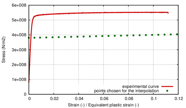
|
| Figure 18: Comparison between the stress strain curve for the uniaxial monotonic tensile test and the points chosen for the numerical model |
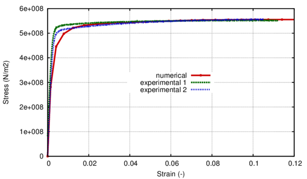
|
| Figure 19: Monotonic stress- strain curve. Numerical vs. experimental. |
The Armstrong- Frederick kinematic hardening function was used for this simulation. The kinematic coefficients chosen were and . In figure 19 the effect of the kinematic hardening on the monotonic curve can be observed. In order to obtain this behaviour a value of 0.1 was used for the parameter.
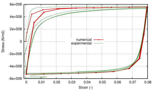
|
| Figure 20: Stress-strain hysteresis loop for =8% Numerical vs. experimental. |
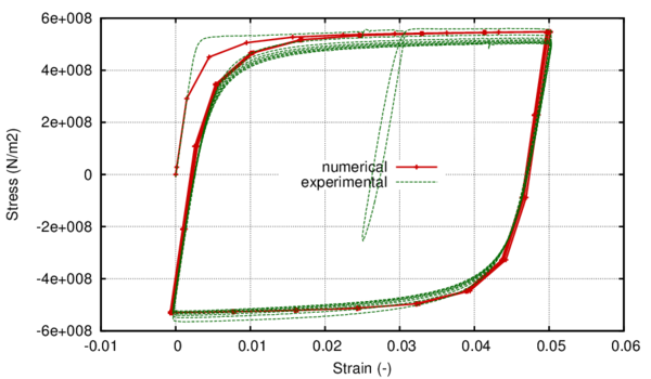
|
| Figure 21: Stress-strain hysteresis loop for =5% Numerical vs. experimental. |
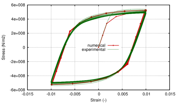
|
| Figure 22: Stress-strain hysteresis loop for =2% Numerical vs. experimental. |
It can be seen that taking into account the kinematic hardening causes the resulting stress-strain curve to elevate until it reaches the experimental monotonic one. Also, the exact shape of the transition zone from linear to nonlinear is determined by the kinematic coefficients.
In figure 21 the numerical hysteresis loop is compared to the experimental one for the =5% case. In choosing the kinematic coefficients a compromise must be made between the accuracy of the monotonic behaviour and of the cyclical one.
Once the kinematic coefficients have been established the next step in the calibration of the material is establishing the equivalent plastic deformation at which softening begins, , and the facture energy.
An experimental result has been chosen for the calibration, the =5% case, that had an experimental fatigue life of 100 cycles. With a value of 13 for the and a fracture energy of 2.7 x 10Nm/m a total fatigue life of 100.35 cycles has been obtained from the numerical simulation. With these values, softening started in the 86 cycle, close to the end of the experimental life and a very low amount of energy was left for the softening branch so that it could be spent in a reduced number of cycles.
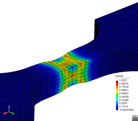
|
| Figure 23: Distribution of the normalized plastic dissipation at total fracture |
In figure 23 the distribution of the plastic internal variable can be seen on the deformed shape of the specimen in the last step of the analysis for the calibration case. The null value for the plastic internal variable represents an elastic state in the material, while means the entire fracture energy of the material has been dissipated at that material point. It can be seen that the lateral necking is in accordance to standard metal fracture under uniaxial cyclic loading.
After the adjustment of the =5% case, simulations were ran with the exact same material parameters and with strain amplitudes of 8%(figure 20) and 2% (figure 22). It can be seen that the considered material parameters offer a good aproximation of the hysteresis loop for these strain amplitudes also. The results in terms of life prediction can be seen in figure 24.

|
| Figure 24: Comparison between numerical and experimental fatigue life for different strain amplitudes when calibrating with =5% |
3.5 Large scale validation on a bent pipe under variable cyclic loading
This section presents the results of finite element simulations made on a bent pipe subjected to an in-plane variable cyclic displacement combined with internal pressure. Special emphasis is put on the capacity of the model to illustrate different failure modes depending on the internal pressure applied on the pipe. The results of the numerical analyses will be compared to experimental ones.
3.5.1 Geometry of the model
Following the validation of the constitutive model made on small scale specimens, the model is to be applied to large scale numerical simulations of a bent pipe. The geometry of the model, boundary conditions and the sequence of loading are in accordance to the experiment made by Schaffrath et al. [105].
The specimens consist of a bended middle section (elbow pipe) and a straight pipe section at each end of the elbow. The fillet radius of the elbow pipe is three times the pipe diameter (R=3 x D). For the length of both straight pipe sections a value of five times the diameter (L=5 x D) was used, whereby the influence of the load introduction can be neglected.
Figure 25 shows the general dimensions of the specimen as a function of the diameter of the pipe, while in figure 26 the geometry of the specimen after manufacturing can be observed. For the numerical simulation, a specimen made of X60 steel has been chosen from the experimental program, with a diameter of 406.4 mm and a wall thickness of 9.5 mm. The pipe has an elbow angle of 90.
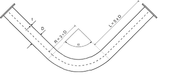
|
| Figure 25: Overview of the general dimensions of the specimen |
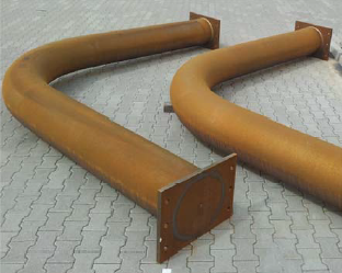
|
| Figure 26: Specimen SP1-SP2 (X60, 90) |
Figure 27 shows the model used for the numerical simulation as generated with the pre-postprocessor GiD. Following, in figure 28 a view of the mesh is shown. For this simulation quadratic hexahedral elements were used, each with 20 nodes and 27 integration points. The mesh consisted of 42853 elements and 213415 nodes. Three elements were considered in the pipe thickness.
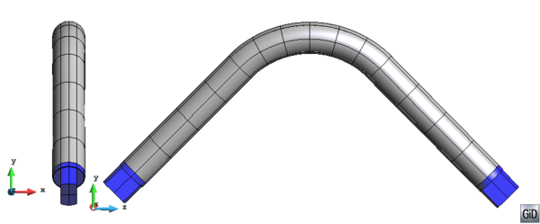
|
| Figure 27: Model geometry |
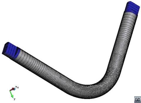
|
| Figure 28: Mesh of hexahedral quadratic elements |
3.5.2 Loading history
The loading history is based on the actual load history of the experimental test done by Schaffrath et al. [105]. The loading scheme was decided by the authors in accordance with the ECCS procedure ECCS-Nr. 45-1986 Recommended Testing Procedure for Assessing the Behavior of Structural Steel Elements under Cyclic Loads [106]. For practical reasons it was decided to neglect the mostly small difference between the compressive and tensile yield strain by choosing an average value as the reference amplitude. In table 3 the experimental loading sequence is described as a function of .The value adopted for this parameter was set by [105] at 82mm.
| Step | Amplitude | Number of cycles |
| 1 | 0.25 | 1 |
| 2 | 0.50 | 1 |
| 3 | 0.75 | 1 |
| 4 | 1.00 | 1 |
| 5 | 1.50 | 3 |
| 6 | 2.00 | 3 |
| 7 | 2.50 | 3 |
| 8 | 3.00 | 3 |
| 9 | 3.50 | 3 |
| 10 | 4.00 | 3 |
| 11 | 4.40 | 27 |
The entire loading sequence is comprised of 49 cycles with increasing amplitude, 44 of which have amplitudes in the plastic range. The reversion factor of the applied displacement is -1 (figure 29). The pipe is also submitted to internal pressure. First, the pipe is loaded until a level of internal pressure equal to 20 bars. Afterwards, it is submitted to the varying cyclic displacement presented in table 3. The experimental test has shown that the internal pressure also oscillates when the cyclic displacement is applied.
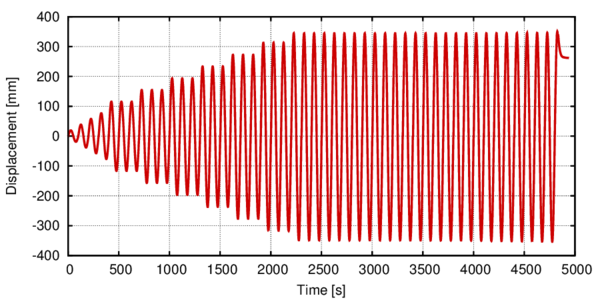
|
| Figure 29: Evolution of the applied displacement in the experiment |
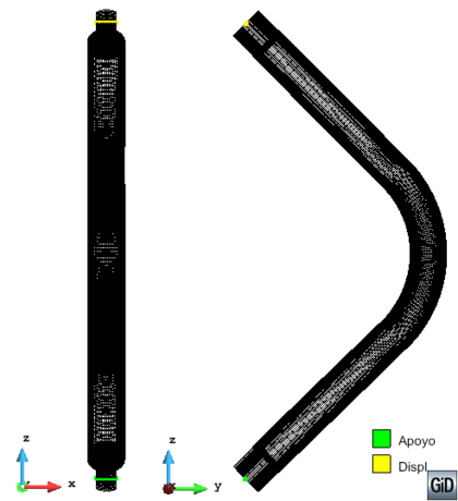
|
| Figure 30: Boundary condition for the large scale model |
In the numerical simulation the loads have been applied in two stages. First, the internal pressure was applied and, in this stage, one end of the pipe was clamped and on the other end the pipe was only allowed in-plane gliding. The variable displacement was applied in the second stage on the deformed geometry obtained from applying the internal pressure. The movement was restrained in the two directions perpendicular to the in-plane one.
3.5.3 Material characteristics
The exact calibration procedure for the X60 material can be seen in Section 3.4.3. In table 4 and table 5 a summary of the material properties as resulting from the calibration can be seen. A polynomial of the 5 degree was chosen for the curve fitting zone of the hardening function.
| Coefficient no. 1 | 380000000,00 |
| Coefficient no. 2 | 326947332,25 |
| Coefficient no. 3 | -861244568,93 |
| Coefficient no. 4 | 1103673406,83 |
| Coefficient no. 5 | -657861660,66 |
| Coefficient no. 6 | 147925577,48 |
| Young Modulus | 1.95 10 | MPa |
| Poisson Modulus | 0.30 | |
| Elastic Stress () | 380 | MPa |
| Plastic Strain Limit for region 1() | 10 | % |
| Plastic Strain Softening () | 1300 | % |
| kinematic hardening | 6.0 10 | MPa |
| kinematic hardening | 400 | |
| Fracture Energy | 2.7 | MN * m/m |
3.5.4 Results and discussion
In figure 31 the comparison between the experimental force- displacement curve and the numerical one can be seen. The numerical curve is in very good agreement with the experimental one taking into consideration that the material calibration was done on small scale specimens with different experimental results.
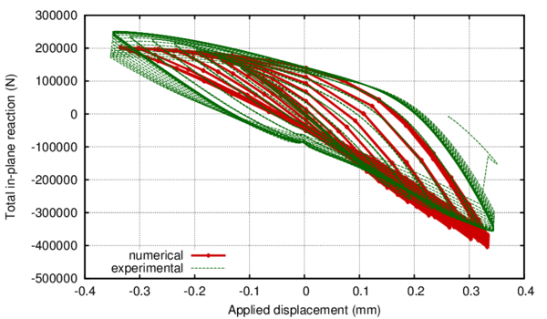
|
| Figure 31: Force-displacement curve. Experimental vs. numerical |
It can be seen how in compression the constitutive equation tends to underestimate the maximum force level, while in traction the opposite tendency is present. Furthermore, this tendency is more obvious as the displacement increases. This is due to the existence of oscillations of the internal pressure applied in the experiment, caused by applying the cyclic displacement. This oscillation of the internal pressure has not been taken into account in the numerical simulation.
Regarding the fatigue life, the simulation lasted a total of 41.75 plastic cycles as compared to the experimental life of 44 complete cycles. This result also shows a good agreement between the experiment and the numerical simulation.
Figure 32 illustrates the deformed shape of the geometry in the last step of the analysis and presents the distribution of the plastic internal variable of the model. The deformed shape is represented with a scale factor of 2 in order to better reflect the general tendency. Only the central zone of the elbow is shown, as this is the zone where nonlinear effects appear. It can be seen that the failure mode resulting from the numerical simulation is by cross-sectional ovalization with a crack opening in the longitudinal direction of the elbow, at its flank.
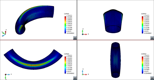
|
| Figure 32: Distribution of the plastic internal variable of the model on the deformed shape (x2) |
In figure 33 the total strain distribution can be seen in the last step of the analysis in the three model axes. The distribution is also plotted on the deformed shape of the model, where the cross-sectional ovalization is clearly visible.
| Figure 33: Distribution of the total strain in the three model axes on the deformed shape of the model (x2) |
It can be seen that strain accumulation occurs in all three directions in the critical area where the normalized dissipation parameter, , accumulates.
The comparison of the failure mode obtained with the numerical simulation with the failure mode obtained in the experimental test (figure 34) shows that the model has been able to capture the number of cycles to failure but has not been able to capture the failure mode shown in the experiment.
Under extreme loading conditions, such as the high repeated incursions in the nonlinear zone that the imposed displacement in this case causes, elbows exhibit two different failure modes. These are either significant cross-sectional ovalization or local buckling, as reported by the experimental work described in Sobel and Newman [107], [108], Dhalla [109] and Greenstreet [110], Tan et al. [111], Shalaby and Younan [112] and Suzuki and Nasu [113] for monotonic bending moments and Yahiaoui et al. [114], Slagis [115]and Fujiwaka et al. [116] for cyclic loading, and from the work of Karamanos et al. [117], [118], Pappa et al. [119], Varelis et al. [120], [121].
An important conclusion can be drawn from the work above mentioned. The first failure mode can be generally found when the elbow internal pressure is relatively low compared to the yield pressure, as is the case in the numerical simulation presented above.
The second failure mode, occurring due to local buckling is habitual in the cases where internal pressure is significantly higher. This is the failure mode yielded by the experiment made by Schaffrath et al. [105] as it can be seen in figure 34.
![Experimental failure (Schaffrath et al. [105])](/wd/images/5/5e/Draft_Samper_124837954-expfailure.png)
|
| Figure 34: Experimental failure (Schaffrath et al. [105]) |
For the case considered, the internal pressure applied to the elbow is 20 bars, which leads to a stress value, according to Barlow's formula: . This is less than 10% of the yield strength for an X60 steel and, consequently, the pressure applied is less than 10% of the internal yield pressure. This puts us in the first yield mode, according to previous results found in literature. The failure due to local buckling obtained for a low value of the internal pressure by Schaffrath et al. [105] can, however, be a consequence of residual stresses generated in the bending process of the pipe combined with local defects that favored the formation of the buckle in the area shown by the experiment and with the effects generated by the oscillation of the internal pressure.
Summarizing, the number of cycles the simulation lasted and the force displacement curve are in good accordance between the numerical model and the experiment and the numerical failure mode is different from the experimental one but justifiable given the low internal pressure imposed in the model.
3.5.5 Considerations regarding the failure mode
In order to assess the capability of the constitutive model to represent both failure modes, a different numerical simulation was done where the internal pressure applied was increased to 220 bars, in order to approximately reach the yield stress. Afterwards, the elbow was subjected to a monotonically increasing in-plane closing displacement.
The model used for this simulation is shown in figure 35. Given the fact that this problem is highly nonlinear and the failure mode expected is achieved thru a local instability (local buckle), in order to achieve convergence when applying the displacement, an initial buckle was imposed on the model. This ensures that, when the internal pressure is sufficiently high, the plastic strain accumulation is directed toward this zone thus enabling model convergence.
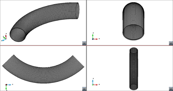
|
| Figure 35: Geometry of the model with the initially imposed buckle |
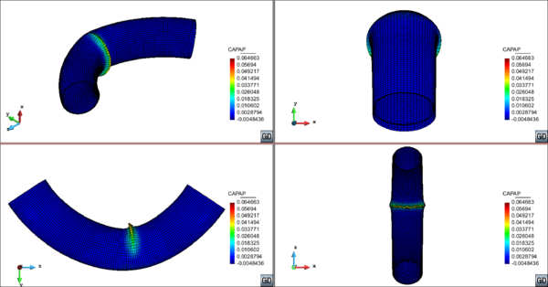
|
| Figure 36: Distribution of the plastic internal variable of the model on the deformed shape |
The final applied displacement up until which the problem converged was 2.69m, nearly 65% of the total in-plane geometry opening. In figure 36 the distribution of the plastic internal variable is shown in the last converged analysis step on the deformed shape of the model with a scale factor of 1, and, as expected, it exhibits a concentration in the imposed buckle zone.
The purpose of this second simulation was to assess the capability of the numerical formulation to illustrate both failure modes in accordance to the level of internal pressure applied.
From the above numerical simulations it is clear that the failure mode obtained with the formulation is highly dependent on the level of internal pressure applied. Taking this into account, a series of six monotonic simulations have been run varying the internal pressure applied initially and applying afterward an in-plane closing displacement. The maximum dissipation zone was assessed when the applied displacement reached the maximum one imposed in the cyclic large scale initial experiment (see table 3).
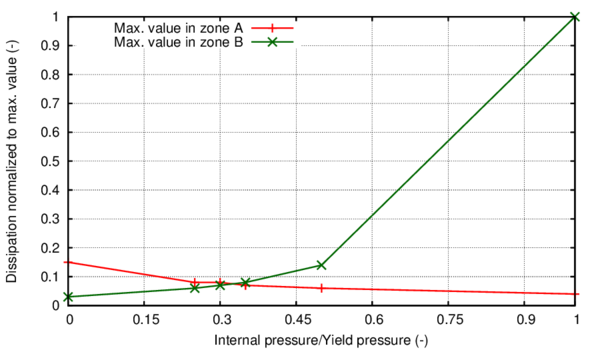
|
| Figure 37: Evolution of the maximum dissipation in the two areas of interest |
In figure 37 the evolution of the maximum dissipation in the geometry is presented in the two areas that are specific to each failure mode: elbow flanks for the ovalization mode (zone A in table 6 and figure 37) and internal elbow curvature for the local buckling (zone B in table 6 and figure 37).
| Py
(%) |
Zone A | Zone B |
| 0 | ||
| 25 | 
| |
| 30 | ||
| 35 | ||
| 50 | ||
| 100 |
From both table 6 and figure 37 it can be seen that the switch from the ovalization failure mode to the local buckling occurs between 30 and 35% of the yield internal pressure, since for the 30% case the maximum dissipation is recorded in the elbow flanks and for the 35% case it is present in the buckled area.
3.6 Large diameter straight pipe loaded monotonically
In order to analyze the capabilities of the constitutive model presented in previous sections, large scale numerical simulations of a straight pipe OD 168.3 x 4.78mm, X52 grade, will be conducted. The geometry of the model, boundary conditions and sequence of loading are established by the experiment made by Coppola et al. [122]. The specimen drawing can be seen in figure 38.
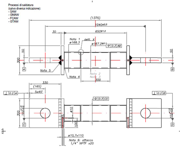
|
| Figure 38: Specimen drawing for X52 full scale testing |
3.6.1 Geometry of the model
The specimen consists of a straight pipe, with three differentiated sections. The central one is mechanized with a reduced thickness, as seen in figure 39 and table 7.
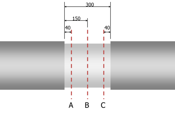
|
| Figure 39: Sections of interest in the mechanization of the straight pipe |
| Wall Thickness [mm] | Outer Diameter [mm] | ||||||
| OD 0 | 164,2 | 163,88 | 164,04 | ||||
| Ref. | sec 1: A | sec 2: B | sec 3: C | OD 45 | 168,3 | 168,5 | 168,42 |
| 0 | 4,24 | 4,18 | 4,36 | OD 90 | 170,57 | 170,65 | 170,34 |
| 45 | 3,85 | 4,19 | 3,99 | OD 135 | 166,89 | 166,64 | 166,04 |
| 90 | 4,01 | 3,91 | 3,77 | ||||
| 135 | 4,24 | 4,05 | 4,10 | WT Avg [mm] | 4,14 | 4,14 | 4,08 |
| 180 | 4,16 | 4,17 | 4,16 | WT Min [mm] | 3,85 | 3,91 | 3,77 |
| 225 | 4,15 | 4,19 | 4,13 | OD Avg [mm] | 167,49 | 167,42 | 167,21 |
| 270 | 4,02 | 4,06 | 4,00 | ID Avg [mm] | 159,22 | 159,14 | 159,04 |
| 315 | 4,41 | 4,37 | 4,16 | Aw [mm, WT Avg, OD Avg] | 2122,06 | 2123,62 | 2092,82 |
| Ki (WT Avg, OD Avg) | 19,765 | 19,732 | 19,985 | ||||

|
| Figure 40: Model geometry in GiD |
In the numerical model the variation in thickness throughout the central zone has been accounted for, as well as the thickness variation throughout the same cross-section. A view of the model geometry in the pre-postprocessor GiD can be seen in figure 40. Following, in figure 41 a view of the mesh is shown. For this simulation quadratic hexahedral elements were used, each with 20 nodes and 27 integration points. The mesh consisted of 8162 elements and 45865 nodes.
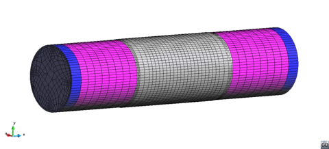
|
| Figure 41: Mesh of hexahedral quadratic elements |
Regarding boundary conditions, shown in figure 42, one capped end of the pipe has its displacement restricted in all directions, while on the other capped end either force or displacement is applied as required by the loading history. When applying internal pressure, one end remains fixed while on the other one the displacement in the longitudinal axis of the pipe is allowed (z-z axis in figure 41) and restrained in the other two directions. The material of the mechanized part is an X52 steel. The outer parts have an elastic material, with the same Young modulus as X52. The pipe caps have been defined as a rigid material in agreement with the setup of the experiment (see figure 38).
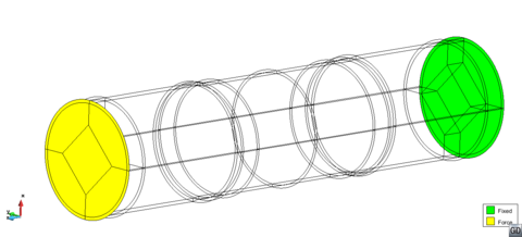
|
| Figure 42: Boundary conditions for the straight pipe |
3.6.2 Loading history
For this simulation two load combinations were made. In the first case (SPEC1) a traction force was applied on one of the caps in the longitudinal pipe axis until a level of 400KN. Afterwards, an internal pressure was applied and gradually increased up to burst. Pipe failure occurred at 270 bars with an associated total axial load of 940KN.
In the second case, the test has been done with internal pressure followed by tension. The internal pressure in the first step is 200 bars. Afterwards, the load was increased up to failure which occurred at 884KN mechanical load (1284KN total axial load). Pressure in the second step was maintained constant at 200 bars. In figure 43 the two loading scenarios are presented.
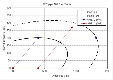
|
| Figure 43: Loading scenarios for the straight pipe |
3.6.3 Material characteristics
The material parameters for the X52 steel have been obtained by undergoing the calibration process described in section 3.4.3 of this document. A polynomial of the 5 degree was chosen for the curve fitting zone of the hardening function. The polynomial coefficients as given by the least squares method are shown in table 8.
The remaining material parameters are shown in table 9.These material parameters were obtained by conducting a calibration process on small scale smooth sample specimens. The geometry of the samples and some calibration results for the cyclic case are presented in section 3.3.
| Coefficient no. 1 | 240000000,00 |
| Coefficient no. 2 | 596993435,99 |
| Coefficient no. 3 | -1019807849,94 |
| Coefficient no. 4 | 776714259,60 |
| Coefficient no. 5 | -265797084,38 |
| Coefficient no. 6 | 33562252,72 |
| Young Modulus | 1.8 10 | MPa |
| Poisson Modulus | 0.30 | |
| Elastic Stress () | 240 | MPa |
| Plastic Strain Limit for region 1() | 15 | % |
| Plastic Strain Softening () | 50 | % |
| kinematic hardening | 6.0 10 | MPa |
| kinematic hardening | 280 | |
| Fracture Energy | 0.4 | MN * m/m |
In figure 44, the monotonic stress strain curve can be seen as obtained with the material parameters presented before. The comparison with the experimental monotonic curves for the X52 steel as obtained from Pereira et al. [101] can also be seen.
Figure 45 exhibits the comparison between the numerical hysteresis loop shape and the experimental one. Although the straight pipe is loaded monotonically, when conducting the calibration analysis for the material, the shape of the hysteresis was one of the factors taken into account as the model is prepared to conduct monotonic and cyclic tests. The calibration process for a monotonic analysis follows the same guidelines as that of a cyclic analysis. The main difference resides in the plastic strain chosen as threshold for the softening behaviour and in the fracture energy assigned to the material.
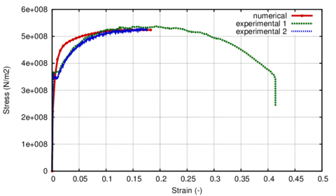
|
| Figure 44: Stress-strain curves for the monotonic case |
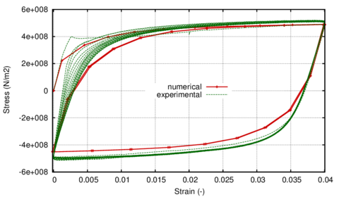
|
| Figure 45: Stress-strain hysteresis loop for =4% Numerical vs. experimental. |
3.6.4 Results and discussion
Case no. 1 - Tension followed by pressure
In figure 46, the comparison between the experimental and the numerical force-pressure measurements can be seen. The total reaction recorded by the numerical simulation reached a level of 948KN in the last converged increment, corresponding to an applied internal pressure of 278.1bars.
For this increment, the deformed shape of the specimen is shown in figure 47, where the distribution of the hardening internal variable can also be seen. This variable is of relevance in showing the level of dissipated energy at material point level and, in this sense, gives a measure of the level of degradation suffered. Consequently, for the material is in an elastic state, while for the material has reached total failure at that material point.
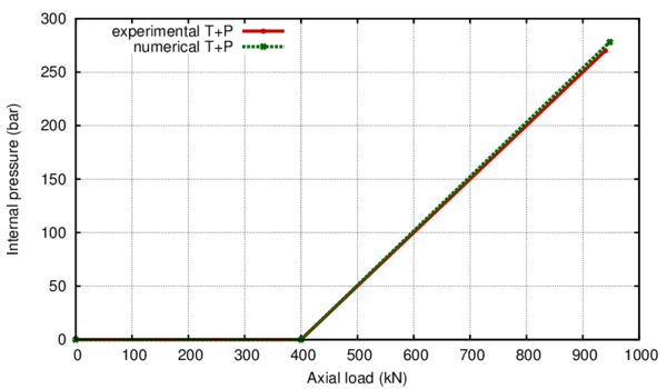
|
| Figure 46: Comparison between the numerical and experimental results for the SPEC 1 case |
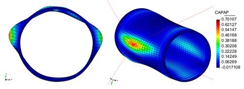
|
| Figure 47: View of the deformed shape at the end of the analysis with an indication of the most damaged material point in the geometry |
From the deformed shape it can be seen that the pipe failure is oriented following the direction of least resistance represented by the minimum thickness area. This is in agreement with the experimental localization of the failure as can be seen in figure 48.
Also, there is good agreement of the failure mode between the experiment and the numerical simulation with a final burst opening oriented in the longitudinal direction. In the numerical model the burst area is represented by the localized plastic strain accumulation reflected in the distribution of the normalized dissipation parameter.
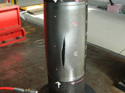
|
| Figure 48: View of the pipe burst as recorded by the experiment for the SPEC1 test |
Figure 49 shows the evolution of the hardening internal variable at the most damaged integration point in the material. Its exact location is indicated in figure 47. As it can be seen from figure 49, the simulation converged up until a maximum value of the internal variable of 0.7. Given that the internal pressure has been applied in constant increments of 2.7 bars per analysis step, it can be seen that the evolution of the parameter exhibits an exponential curve. Taking into account this tendency and extrapolating on the last converged increment that had a value of 0.7, loss of convergence seems to have occurred when the plastic internal variable reached a value very close to 1, corresponding to an open crack generated at the material points where the entire fracture energy of the material has been spent. However, this value is not visible in figure 49 since convergence was not reached for this increment.
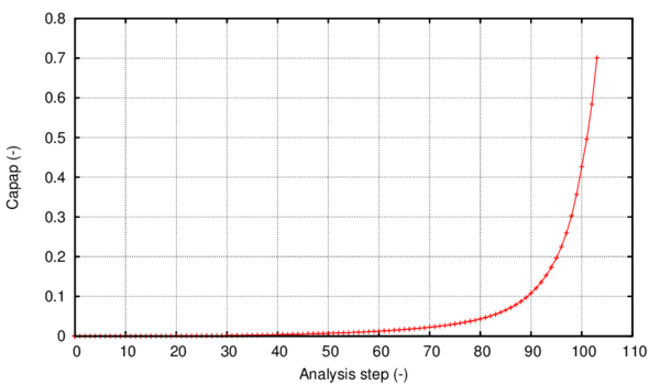
|
| Figure 49: Evolution of the variable when applying internal pressure in constant steps of 2.7 bars |
Case no. 2 – Internal pressure followed by tension
In figure 50 the comparison between the experimental and the numerical force-pressure measurements can be seen for this case.
The total reaction recorded by the numerical simulation reached a level of 1167KN in the last converged step, corresponding to a total applied displacement of 1.375m. The experimental failure occurred at a total axial load level of 1284kN.
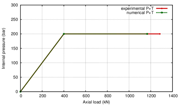
|
| Figure 50: Comparison between the numerical and experimental results for the SPEC 2 case |
As specified before, during the applied displacement stage the internal pressure was maintained constant at a level of 200 bars. For the last step of the simulation the deformed shape is shown in figure 51, where the distribution of the hardening internal variable can also be seen.
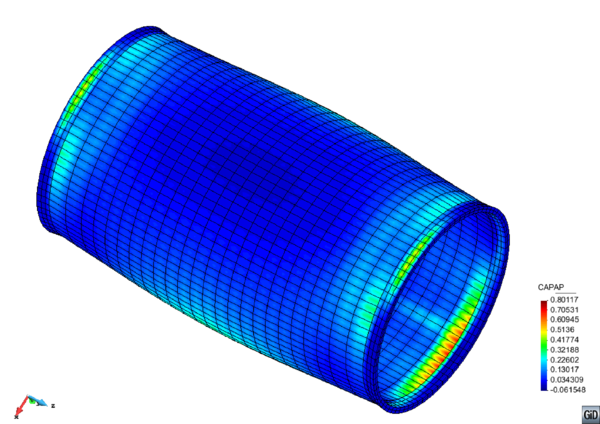
|
| Figure 51: View of the deformed shape for the SPEC 2 case |
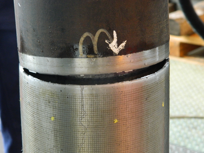
|
| Figure 52: View of the pipe burst as recorded by the experiment for the SPEC2 test |
The localization of the failure zone corresponds to the behaviour shown in the experiment, presented in figure 52. When considering the pipe cross section where the maximum dissipation is present, the most stressed area is directed towards the smallest thickness in that particular circumference, corresponding with the data recorded by the experimental campaign and taking into account the orientation of the numerical model with respect to that of the experimental setting. The failure mode is a tensile one, in agreement to the applied sequence of loading.
3.7 Advantages of the approach proposed
Previous results have shown that the proposed constitutive model is capable of predicting material failure after applying several cycles to the material.The formulation is also capable of predicting the structural failure under monotonic loads. However, this prediction capability do not present a major advantage compared to other approaches such as the Coffin-Manson rule, or any other analytical expression capable of defining the maximum number of cycles that can be applied for a given plastic strain.
The main advantage of the proposed approach is that the prediction of ULCF failure does not depend on the applied plastic strain, but on the energy dissipated during the cyclic process. Therefore, it is possible to vary the plastic strain in the cycles applied to the structure and the constitutive model will be still capable of predicting the material failure.
This is proved in the following example, where an irregular load, in frequency and amplitude, is applied to the SP sample defined in section 3.3 and used to validate the formulation. The load defined is depicted in figure 53.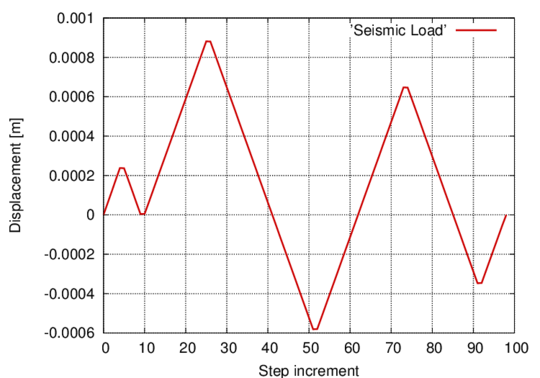
|
| Figure 53: Seismic-type load applied |
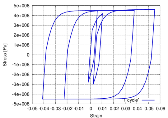
|
| Figure 54: Material stress-strain response |
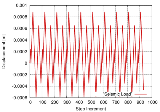
|
| Figure 55: Seismic-type load applied: ten seismic-type cycles |
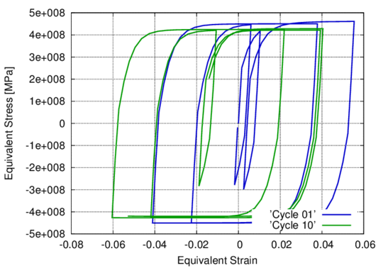
|
| Figure 56: Material stress-strain response after ten seismic-type cycles |
The model is capable of capturing the energy dissipated in each one of these loops and, therefore, to evaluate the energy available in the material after having applied the load, which is equivalent to the residual strength of the material. It is also possible to repeat several times the irregular load, as shown in figure 53, to study the number of repetitions that are required to reach material failure. Figure 56 shows the stress-strain response of the material after 10 cycles (figure 55). At this point there are some points in the model that have lost most of their fracture strength and specimen failure occurs. As occurred with the SP model, this simulation also shows some lateral displacement on the equivalent strains due to the plastic strains suffered by the whole specimen.
4 Constitutive modelling of High Cycle Fatigue
4.1 Introduction
A stepwise load-advancing strategy for cyclic loading will be presented in this chapter that yields convergence in reasonable computational time for highly nonlinear behaviour occurring past the S-N curve. The algorithm is also effective when dealing with combinations of cyclical loads. The strategy is coupled to a continuum damage model for mechanical fatigue analysis. An overview of the constitutive model is also presented. The capabilities of the proposed procedure are shown in several numerical examples. The model is validated by comparison to experimental results.
The basis of the HCF constitutive model used was initially developed by Oller et al. [2]. The model establishes a relationship between the residual material strength and the damage threshold evolution, controlled by the material internal variables and by a new state variable of fatigue that incorporates the influence of the cyclic load. A brief overview of the constitutive formulation for the HCF case is provided in order to clarify the material behaviour exhibited in the numerical examples. Several model assumptions are to be made. Defect concentration on the microscale occurs during the whole period of cyclic loading. This is reflected in the model in a continuous reduction of the material strength, occurring even in the elastic stage. Stiffness degradation occurs only in the post critical stage, once the curve has been passed and, therefore, only in the final stage before failure. The damage parameter has a phenomenological significance indicating the irreversibility of the fatigue process.
Depending on the size of the domain chosen for a fatigue numerical simulation, computational time for a numerical analysis can vary considerably. Nowadays, running simulations at macroscale level (mechanical part, structural element) continues to be a challenge, especially if the high level of structural complexity attained at the microscale needs to be taken into account to some extent at other scales. This work offers a stepwise load-advancing strategy that allows a saving of computational time and can help push the barrier of what if possible in terms of numerical simulation one step further.
The strategy can be especially effective when dealing with HCF where material lives are in the range of 10 – 10 cycles. If a single loading cycle is described by n loading steps and the structure fails at 10 cycles, then the number of loading steps required to complete a HCF analysis would be in the order of 10 x n. Furthermore, if the mechanical piece has a complex geometry and a high level of discretization is required at finite element level, then at each of the 10 x n load steps a large number of constitutive operations need to be computed for each integration point. The above serve as a clear example of why load-advancing strategies are of the utmost importance in HCF simulations.
Furthermore, increasingly more attention has been given to material behaviour in the very high cycle regime from an experimental point of view. The general belief that steel experiences no alteration in its properties after reaching its fatigue limit at 10 cycles has been invalidated [123], [124], [125]. In this context, this work provides a tool for rapid automatized time-advance that allows taking numerical simulations beyond the limit of 10 cycles in reasonable computational time with the added benefit of being able to predict fatigue failure when dealing with combinations of different cyclical loads and also of being able to evaluate the residual strength of the material once a cyclical load has finished.
4.2 HCF damage model
A description of the constitutive model is offered in this section. The fundamentals of a fatigue continuum damage model are presented with a clear emphasis on the dependence of the model on the S-N curves. An exhaustive description of the formulation used can be found in Oller et al. [2], where the complete thermo-mechanical constitutive model for the prediction of fatigue effects in structures is formulated. The model is capable of taking into account the effect of the mean stress. The treatment of the highly complex processes generated by fatigue is made from a phenomenological point of view.
4.2.1 Mechanical damage formulation
The free Helmholtz energy is formulated in the reference configuration for elastic Green strains, , as [92]:
|
|
(33) |
where is the material density, is the total strain tensor, is the internal damage variable taking values between its initial value 0 and its maximum value 1 and is the initial constitutive tensor.
Considering the second thermodynamic law (Clausius-Duhem inequality – [94] [91] [95]), the mechanical dissipation can be obtained as [92]
|
|
(34) |
The accomplishment of this dissipation condition (Equation 34) demands that the expression of the stress should be defined as (Coleman method; see [95])
|
|
(35) |
Also, from the last expressions, the secant constitutive tensor can be obtained as:
|
|
(36) |
where is the stress tensor for a single material point.
4.2.2 Threshold damage function oriented to fatigue analysis. Phenomenological approach
The effects caused by applying an increasing number of loading cycles are taken into account by means of a proposed function. This function is introduced in the above formulation in the expression of the damage threshold surface, , proposed by [95], [126] and [127]. The number of cycles N can then be incorporated as a new variable. This enables the classical constitutive damage formulation to account for fatigue phenomena by translating the accumulation of number of cycles into a readjustment of the damage threshold function.
The non-linear behaviour caused by fatigue is introduced in this procedure implicitly, by incorporating a fatigue state variable, , that is irreversible and depends on the number of cycles, the maximum value of the equivalent stress in the material, , and on the factor of reversion of the equivalent stress, . This new variable affects the residual strength of the material by modifying the damage threshold, , either on the equivalent stress function (equation 37), or on the damage strength threshold (equation 38) [2].
|
|
(37) |
|
|
(38) |
In the above, , is the reduced equivalent stress function in the undamaged space, is the fatigue damage strength threshold, and the damage internal variable. In the following, the form in equation 37 has been used for the damage threshold criterion.
The evolution of the damage variable is defined as:
|
|
(39) |
being the consistency damage factor, which is equivalent to the consistency plastic factor defined in [92]. Consequently, for the isotropic damage case,
|
|
(40) |
4.2.3 Particularization of the damage threshold function for exponential softening
The type of softening to be defined in the general damage criterion depends on the problem to be solved. The scalar function defining the evolution of the damage threshold must be monotonous and with a value ranging from 0 to 1. In various publications about the scalar damage problem, the stress behaviour with softening is represented in a variety of forms. Particularly, in Oliver et al. [127] the following function is proposed,
|
|
(41) |
This function can also be expressed as,
|
|
(42) |
where is a parameter that depends on the fracture energy of the material and . The value of is obtained from the fulfilment of the damage criterion for the first threshold of degradation. This complies with , and .
The A parameter is calculated from the dissipation expression shown in equation , particularized for a uniaxial process subjected to a growing monotonic load. The parameter deduction can be obtained from [98] and has the following expression for exponential softening:
|
|
(43) |
4.2.4 Function of residual strength reduction for fatigue – Wöhler curve definition
Wöhler or Stress-Number of cycles (S-N) curves (figure 57) are experimentally obtained by subjecting identical smooth specimens to cyclic harmonic stresses and establishing their life span measured in number of cycles. The curves depend on the level of the maximum applied stress and the ratio between the lowest and the highest stresses (R=S/S). In figure 57b S is the endurance limit for a reversion factor of -1 and is the material elastic limit. In figure 57a the instantaneous stress level is depicted, while in figure 57b the cyclic stress is represented only by the maximum value it reaches in every cycle. Usually, S-N curves are obtained for fully reversed stress (R=S/S=-1) by rotating bending fatigue tests.
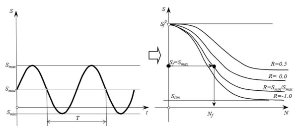
|
| Figure 57: a: Stress evolution at a single point; b: (Wöhler's) Curves |
curves are, therefore, fatigue life estimators for a material point with a fixed maximum stress and a given ratio R. If, after a number of cycles lower than the cycles to failure, the cyclic load stops, a change in the elastic threshold of the material is expected due to accumulation of fatigue cycles. Furthermore, if the number of cycles exceeds Nf, being Nf the fatigue life as resulting from figure 58, the material will fail with the consequent reduction of strength and stiffness. The change in strength is quantified by the strength reduction function, , while the change in stiffness is taken into account by means of the damage parameter. In figure 58, S is the endurance limit for any given reversion factor and S is the elastic threshold limit.
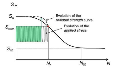
|
| Figure 58: Schematic representation of the evolution of the residual strength with the applied load and number of cycles |
In the case of a cyclic load with constant S and R throughout the entire life of a material, the curve is sufficient for determining fatigue life. However, when dealing with different load interactions the main focus resides on the residual strength curve. The curve quantifies the loss of strength in the material as the number of cycles accumulates and as load characteristics change.
All fatigue numerical simulations are based on the Wöhler curves obtained experimentally. These curves are described in an analytical form with the help of material parameters. Their expression, as well as the analytical definition of the strength reduction function, is connected to the experimental curve and, therefore, subjected to change if the material changes. Different analytical definitions can be found in [128], [129] and [130], as well as in [2].
Here the analytical fomulation presented in [2] is shown.
Based on the actual value of the R ratio and a basic value of the endurance stress (for ) the proposed model postulates a threshold stress . The meaning of is that of an endurance stress limit for a given value of R=S/S.
|
|
(44) |
If the actual value of R is then, . The effect of the number of load cycles on the ultimate stress for a given value of R is taken into account by an exponential function,
|
|
(45) |
The value of is given by the function,
|
|
(46) |
where and are material parameters that need to be adjusted according to experimental tests. Figure 59 shows an example of application of these functions. Parameters were chosen as follows: , , , , , and .
| [[ |
| Figure 59: Proposed curves for different values of . [2] |
The proposed curves, equations 44 - 46, are fatigue life estimators for a material point with a fixed maximum stress and a given ratio . If, after a number of cycles lower than the cycles to failure, the constant amplitude cyclic load with a maximum stress (and ratio ) is removed, a change in is expected due to the accumulation of fatigue cycles. In order to describe that variation of the following function is proposed:
|
|
(47) |
where is one of the parameters of equation 45 and is obtained as a function of the ratio and the number of cycles to failure , by:
|
|
(48) |
The value of can be obtained from equation 45:
|
|
(49) |
Some important observations have to be made regarding the fatigue strength reduction function. Habitually, fatigue models are limited to correctly describing the curves and, based on the level of stress applied, estimate the fatigue life. The curve is generally interpreted as a life prediction tool, meaning that when, for a certain level of stress, the corresponding to the Wöhler curve has been reached the respective Gauss point has suffered complete degradation. However, the present model utilizes the respective point as the starting point for damage accumulation and the nonlinear zone, for that particular Gauss point. This event mirrors the initiation point for a microcrack. Posterior damage accumulation is an indicator of a rearrangement of the internal structure of the material followed by micro-fisuration and a completely degraded Gauss point () represents the formation of a macro-crack in the volume associated to the integration point. At macroscale level, a tracking of the damage propagation throughout the continuum is an indicator of a crack propagation and total structural rupture is considered to have occurred when the crack has propagated thru the entire cross-sectional area.
The analytical formulation mentioned above has been coupled with a signal processing routine so that random cyclical loading can be decomposed into different load sections, each described by its characteristics: amplitude, reversion factor, number of cycles, period. The residual strength curve quantifies the reduction in material strength due to the application of each loading section in a particular order, as will be shown in the numerical examples presented later on in this chapter.
4.3 Stepwise load advancing strategy
4.3.1 Introduction
The stepwise load-advancing strategy proposed in this chapter uses the formulation described previously and consists of two different phases. The first one is defined by load-advance being conducted by small time increments, with the consequent load variation following a cyclic path. The second phase is characterized by load-advance being done with large increments of number of cycles.
Even though Oller et al. [2] described the possibility of advancing thru large increments of number of cycles, the process was not automatic. This implied that it could not be used in real life simulations where an in-depth tracking of the material's progressive degradation was desired, or where the loading history was comprised of several different cyclical loads.
This work proposes an algorithm that automatically switches from one phase to the other, going repeatedly back and forth between both in accordance with the loading input and the damage increase rate.
4.3.2 Load-tracking phase
This phase is characterized by the load being applied in small increments. The purpose is to determine and save the characteristics of the cyclical load. The tags Ai referenced in the following can be seen in the flow chart for this phase, on the left side of figure 60.
Each load cycle will be divided into m small steps, a value that is user defined. At the beginning of each increment being conducted in this phase, both the load factor and the number of cycles will be updated (A1). Based on the multiaxial stress state, the equivalent stress will be computed according to the damage criterion chosen (von Mises, Mohr-Coulomb, Tresca, Drucker-Prager). After that, the difference between the equivalent stress of current increment k and previous increment k-1 will be compared to the difference between the equivalent stress in k-1 with respect to k-2 (A2)(See figure 60). When the sign of these two quantities is different, either a maximum or a minimum has been recorded in increment k-1(A3). After having detected both the maximum and the minimum equivalent stress for each integration point, the reversion factor is computed, R=S/S. After each new cycle i+1 is described, the reversion factor is compared to its value in the previous cycle i. The normalized variation of the reversion factor is evaluated for each integration point GP and the sum of all the variations detected is computed into a stabilization norm as shown in equation 50 (A4).
|
|
(50) |
A new value for is computed and the equivalent stress is then affected by it and compared to the damage strength threshold in the current increment (A5). The check for global convergence is made and, if this is achieved, then the stabilization norm is compared to a user defined tolerance. When this norm is below a given tolerance, it can be said that the reversion factor has a stable value throughout the solid (A6). A flag is then activated indicating that in the next increment the large phase algorithm should be followed. If the value of is not below the tolerance, several more cycles are then analysed applying small increments.
This phase is necessary at the beginning of each different cyclical load in order to determine the parameters that define the cyclic behaviour at each Gauss point of the structure (R and S). Therefore, in case of modifying the cyclic load, a new activation is necessary.
4.3.3 Large increments phase
After the stress parameters, R and S, stabilize throughout the solid from one cycle to the other, there is no need to keep applying small increments as there will be no change in the stress state unless either the elastic threshold is reached or the applied cyclical load changes. Therefore, the load level can be maintained at its maximum value and large increments of number of cycles can be applied. The tags Bi referenced in the following can be seen in the flow chart for this phase, on the right side of figure 60.
In this phase the variable is not the level of the load, kept constant at its maximum value, but the number of cycles, which, in each increment, is updated with a new large Nc step (B1). After obtaining the equivalent stress, a new value for is computed directly with the current number of cycles and the previously stored values for R and S (B2).The equivalent stress affected by is then compared with the current damage strength threshold. If nonlinear behaviour occurs at at least one integration point a flag is activated (B3). When global convergence of the problem has been obtained in the current increment and the flag has been activated inside the constitutive loop, the next increment will be conducted with the load-tracking algorithm (B4).If convergence has been reached but the flag was not activated, in the next increment another large step will be applied.
4.3.4 Automatic load-tracking phase activation
The stepwise advancing strategy has the following implications:
When applying a single cyclical load, load advance will be done by passing initially thru the load-tracking phase until R stabilizes and is lower than the defined tolerance. Afterwards, the advancing scheme will be by number of cycles until reaching the elastic threshold. This happens when the material has been subjected to the number of cycles indicated by the S-N curve. At this stage, the internal forces of the structure are modified in order to reach a new equilibrium configuration. This situation leads to a variation of the reversion factor and, therefore, of the stress state at integration point level. The load-tracking phase is automatically activated. Furthermore, it will be activated at each step where damage increases () due to the change in internal forces.
The algorithm can be optimized if, after evaluating the Wöhler's Nf (marked dot in figure 58) corresponding to each equivalent stress level at the beginning of the analysis, a search is made to find the minimum fatigue life throughout the solid. The resulting number of cycles can be used as the first step of the large increments phase ensuring that the entire span of number of cycles before the damage process initiates is done in one step (B1)(See figure 60). The nonlinear processes occurring past the point damage initiates in the first Gauss point will be simulated with a user-defined N step in the case of displacement controlled simulations where the material can continue bearing the cyclical load after having reached the fatigue life given by the S-N curve. This is possible due to a progressive loss of stiffness that ensures that, for the same applied cyclical displacement and having reached the S-N curve, stress in the material progressively relaxes as it suffers damage until total rupture.
In the case of applying different cyclic loads, damage can appear either due to fatigue or due to a new load being applied that leads to stress values that surpass the elastic threshold. In both cases the model will jump automatically from the large increments phase to the load-tracking phase. Even if the different cyclic loads applied induce stress levels below the elastic threshold, when passing from one cyclic load to another one of different characteristics an activation of the load-tracking is required. This is necessary regardless of the elastic regime due to the fact that, by applying a new load, the maximum equivalent stress induced and/or the reversion factor has changed and, consequently, the fatigue parameters calculated for the first load are no longer valid.
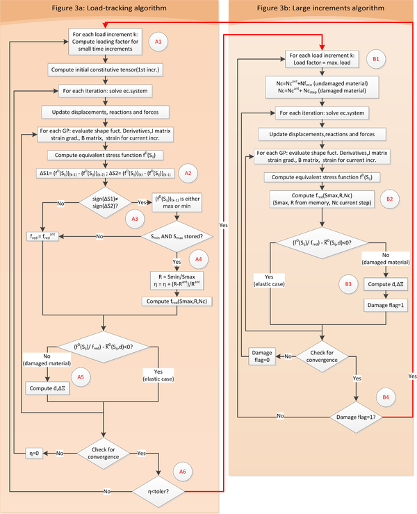
|
| Figure 60: Flow chart for the stepwise advancing algorithm |
The flow chart presented in figure 60 shows the operations conducted in both phases, as well as the conditions required to jump from load-tracking to large increments. These jumps are indicated with hyphenated arrows.
The algorithm is user controlled by means of two parameters. The first one is the tolerance at which the reversion factor norm (defined in equation 50) is considered to have converged. If, for instance, a numerical tolerance of 10 is used, time advance runs the risk of being continually conducted in the load-tracking phase. This would lead to a dramatic increase in computational time. On the other hand, if the tolerance is set too high the model may no longer capture changes in the cyclical load applied, leading to an incorrect life prediction. The tolerance used for the calculation of the numerical examples presented in section 4 was 10 and the author recommends this value for future use of the strategy.
The second parameter that allows the user to control the developed stepwise load advancing algorithm is the number of cycles chosen as time step for the large increments phase. The influence it has is in accordance with the level of nonlinearity of the problem. While a too low number of cycles used as step implies an increase in computational time, a too big one can lead to loss of solution convergence. A calibration analysis consisting of a study of the solution convergence depending on the number of cycles used as a step is highly recommended. The analysis should begin by using large steps. Then the N used as a step should be progressively lowered until convergence is reached, as this would ensure the lowest computational time.
4.4 Numerical examples
The capabilities of the stepwise load-advancing strategy, together with the fatigue constitutive model presented, will be shown with several simulations made over a hexahedral finite element subjected to cyclic loads. These examples will illustrate the fatigue behaviour under a single cyclical load and under load interaction of two different cyclic loads. Also, the material behaviour is shown when combining a cyclical load with a monotonic one. After that, the model is validated comparing the results obtained from the numerical simulation with the results provided by the experiment presented in Marines et al. [131].
All the examples presented in this section have been calculated with the PLCd finite element code [102], where the formulation presented here has been implemented.
In order to understand the capabilities of the stepwise load advancing strategy, a test case of one linear hexahedral element with 8 integration points will be presented. A single element was chosen for the simulation due to its reduced computational cost and due to the fact that it suffices for accurately showing material behaviour as described by the formulation presented.
4.4.1 Problem definition. Geometry, material and boundary conditions.
The element has one of its faces subjected to a cyclical displacement while the opposite face has boundary conditions that fix its longitudinal displacement, allowing transversal expansion and contraction.
Geometry dimensions are . The material used has the following characteristics: Young modulus = 2.01 x 10 MPa ; Poisson ratio = 0.3 ; Static elastic threshold is S = 838.9MPa and the material fracture energy has a value of G = G = 20 kN*m/m . The damage model used has exponential softening and a Von Mises failure surface. The curve for this material was obtained using the analytical formulation described in [129]. The parameters required in order to correctly describe the curve are S, S and R.
One of the model's particularities is the progressive loss of resistance leading to the initiation of damage, represented in the strength reduction curve. In order for it to be clearly differentiated from the Wöhler curve, a direct jump to the point where damage initiates was not done. Rather, an approximation of the damage initiation point was made by choosing a suitable number of cycles as the time step.
The first two numerical simulations presented exhibit a load history composed of a single cyclical load, while the last two simulations consist of applying both cyclical loads in different order.
The characteristics of the cyclical loads taken into account are: for the first one, , a reversion factor of 0.3, a minimum displacement of 0.0114mm and a maximum displacement of 0.038mm; in the second case, , the first load applied has a null reversion factor, a maximum displacement of 0.035mm and a null minimum displacement. The number of cycles adopted as a step for the large increments phase in the both cases is 10 cycles.
For the combination cases the load applied is the first one, , and, after 10 cycles, this load is replaced by . The number of cycles used as a step for the large increments phase in this case is 10 cycles. In the second combination case the order of loads applied has been changed. First, load 2 is applied 10 cycles and afterwards the material continues to be loaded with load 1 until total failure. The number of cycles adopted as a step for the large increments phase in this case is also 10 cycles.
4.4.2 Single cyclical load
Table 10 shows the stresses obtained at each integration point by the imposed displacement presented in figure 61, as well as the fatigue life provided by the FEM model.
| (normalized with threshold limit) | |||||
| Case code | Reversion factor | Max. Stress PG | Min. Stress PG | Med. Stress PG | Nc when damage initiates |
| 0,3 | 0,91 | 0,273 | 0,59 | 4,90E+06 | |
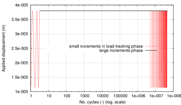
|
| Figure 61: Applied displacement for load case |
The stresses induced by the cyclic displacement applied lead to a fatigue life, according to the material Wöhler curve, of 4,9 x 10 cycles. This number of cycles marks the beginning of the nonlinear process and, therefore, of the energy dissipation.
In figure 62, the stress in the specimen, the material Wöhler curve, the residual strength variable and the material damage value are presented. It can be seen that, while the residual strength curve is above the Wohler fatigue life curve, there is no stress alteration or damage accumulation.
The stress level shown refers to the instantaneous stress divided by the initial elastic threshold. It can be seen that at the beginning an initial load-tracking stage is necessary for recording the characteristics of the stress evolution: reversion factor, maximum stress value and stress amplitude in every cycle. When the cyclic stress characteristics do not change from one loading cycle to the other (at every Gauss point) large increments start to be applied, where the load is maintained at the maximum value reached in previous cycles and only the number of cycles variable increases. At this point the material is considered to be in an elastic state but the evolution of the S-N and of the residual strength curves continues to be monitored.
Once the number of cycles applied reaches the fatigue life defined by the Wöhler curve for that level of maximum stress, event marked by the stress curve intersecting the Wöhler curve, it also intersects the residual strength curve. After this point, the stress in the material is higher than the residual strength and a softening process begins with the consequent increase of the damage variable. As soon as this event occurs at the first Gauss point a load-tracking stage is automatically activated for the entire finite element model. This is necessary as the onset of the degradation process leads to a change in the internal forces and a new equilibrium configuration is reached. When this equilibrium configuration has stabilized under small increments, the stress characteristics from one cycle to the other remain constant. This enables the application of a large increment, maintaining the load at the maximum level reached in previous stable cycles. However, when applying this large increment the equilibrium is lost again as the structure is pushed further in the nonlinear zone with a consequent damage accumulation and stiffness loss. This effect can be seen in the stress relaxation occurring at the end of each large scale increment (figure 62 and figure 63).
From that point forward, after each large increment where , the load-tracking phase is automatically activated so that damage evolution can be monitored from cycle to cycle. If, after describing several cycles with small increments, the stress state throughout the solid has stabilized, a new large increment can be applied. This process is repeated automatically until the material reaches a state of complete degradation.
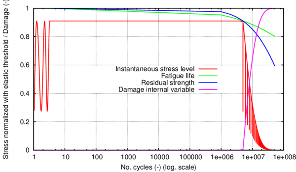
|
| Figure 62: Parameters of interest for the fatigue analysis under load |
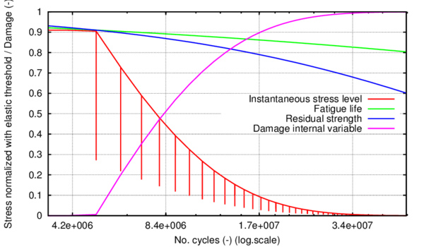
|
| Figure 63: Parameters of interest for the fatigue analysis under load in the nonlinear zone |
Figure 63 zooms the end part of figure 62 to show more clearly the material performance described. The load-tracking phase is represented by the vertical lines. The large increments phase is represented by the in between segments. Both figure 62 and figure 63 have a logarithmical scale along the horizontal axis.
In figure 64, the effects of material degradation are shown in the stress-strain curve. The vertical axis refers to the instantaneous stress level divided by the material elastic limit. The large increments phase occurs only when the displacement is maintained at its maximum value and . Therefore, it is represented in this figure by the vertical lines descending from the point of maximum stress. The stress interval represented by each jump in the stress level quantifies the stress softening caused by a single, large number of cycles, interval. Each of these stress-softening intervals is followed by a few unloading (until minimum displacement) - loading cycles. These mark the load-tracking phase where a clear change in material stiffness is visible.
It can be seen that, as the material progressively suffers loss of stiffness, for the same large step there is less stress softening.
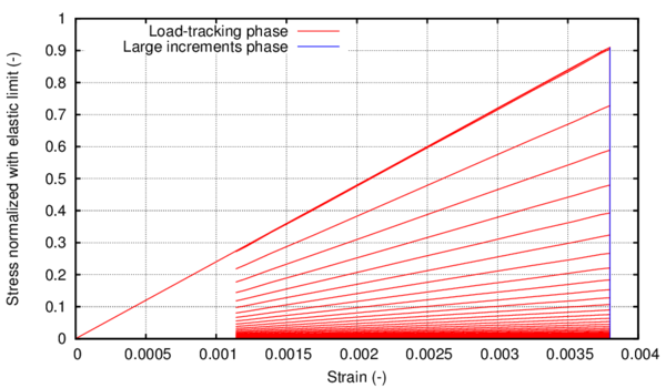
|
| Figure 64: Stress-Strain at integration point for load |
Furthermore, in order to demonstrate the good accuracy of the method, this simulation has been done with four different sizes for the large increments phase. Figure 65 presents the evolution of the damage internal variable (as resulting from equation 40) with the number of cycles in all four cases. It can be seen that, even though the simulation is done by using different steps in the large increments phase: 50.000, 100.000, 1 x 10 and 5 x 10 cycles, the damage variable has the same evolution.
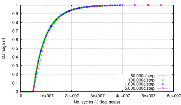
|
| Figure 65: Evolution of the damage internal variable with the number of cycles |
As indicated in Section 4.3.4 the number of cycles used as a step in the large increments phase is a key parameter for the load-advancing algorithm. In table 11 the computational time obtained for the different N steps is presented. It can be seen that, even though the simulation is made on a single linear element, computational time can vary considerably depending on the number of cycles chosen as time step.
| No. of cycles considered as step | 50.000 | 100.000 | 1 x 10 | 5 x 10 |
| CPU time | 0h: 8':42 | 0h: 4': 8 | 0h: 0':30 | 0h: 0':10 |
A comparison was made between the computational time required when using the proposed load-advancing strategy and the computational time needed if in the nonlinear stage only load-tracking were to be used. As it can be seen from table 11, the CPU time needed in the case of a step of 1 x 10 cycles was 30 seconds for a total analysis of 53.5 x 10 cycles, out of which 4.9 x 10 cycles consisted of elastic behaviour. When advancing only by load-tracking after the 4.9 x 10 elastic cycles, in 10 hours of computational time only 84.000 cycles were computed, with a correspondant damage level at the end of the 84.000 cycles of 0.018. Taking into account this rate of advance, if the entire analysis of 53.5 x 10 cycles were to be conducted under load-tracking, a computational time of 265 days would be needed. This study was carried out on only one linear element. In real-life simulations, the dimensions of the problem are much larger and load history is more complex and this demonstrates that it is of the upmost importance having a load-saving advancing strategy.
An important feature of the constititutive model coupled with the load-advancing strategy is the ability to account for the order in which different loads are applied within a determined load history. In order to demonstrate this, a different regular cyclic load will be shown and, in the next section, the combination of the two loads, and will be analysed.
The characteristics of the tensional state induced by the load are shown in table 12. In figure 66, the stress evolution at the integration point, the material Wöhler curve, the residual strength variable and the material damage value are presented, and in figure 67 the effects of material degradation are shown in the stress-strain curve.
| (normalized with threshold limit) | |||||
| Case code | Reversion factor | Max. Stress PG | Min. Stress PG | Med. Stress PG | Nc when damage initiates |
| 0 | 0,839 | 0 | 0,42 | 3,46E+06 | |
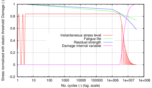
|
| Figure 66: Parameters of interest for the fatigue analysis under load |
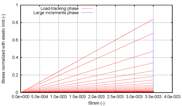
|
| Figure 67: Stress-Strain at integration point for load |
4.4.3 Load history with two different cyclical loads
In table 13 the stresses generated at integration point level by the imposed maximum and minimum displacements are included. These are displayed for the two cyclical loads applied, and , as well as the fatigue life resulting from the FEM model if only one of the loads, be it or , were to be applied until fracture. Table 13 also includes the number of cycles at which damage starts when applying both and .
| (normalized with threshold limit) | |||||
| Case code | Reversion factor | Max. Stress PG | Min. Stress PG | Med. Stress PG | Nc when damage initiates |
| 0,3 | 0,91 | 0,273 | 0,59 | 4,90E+06 | |
| 0 | 0,839 | 0 | 0,42 | 3,46E+06 | |
| + | 3,62E+06 | ||||
| + | 1,22E+06 | ||||
The simulation of the load combination was made by first imposing the load during 10cycles, followed by load being applied from 10 cycles to 10 cycles. By applying first load , followed by load , the resulting life for the material is 3,62 x 10 cycles, less than if only load were applied, but more than if only were applied. This shows that the formulation is capable of taking into account the effect of a cyclical load even if it is applied for a number of cycles that does not lead to failure. This is achieved by quantifying the strength reduction caused by each event in the load history and by dynamically describing the curve according to changes in load characteristics.
In figure 68 it can be seen how the slope of both curves, residual strength and curve, changes as a different load starts being applied. This is possible due to the load-tracking phase being automatically activated once a change in the load is detected, as can be seen from the vertical line dividing the two maximum stress levels exhibited. The intermediate load-tracking phase appears as a straight line due to the fact that a logarithmical scale has been used for the horizontal axis. The characteristics of the new load are consequently determined, maximum stress level and reversion factor, and with these parameters the and reduction curve readjust themselves.
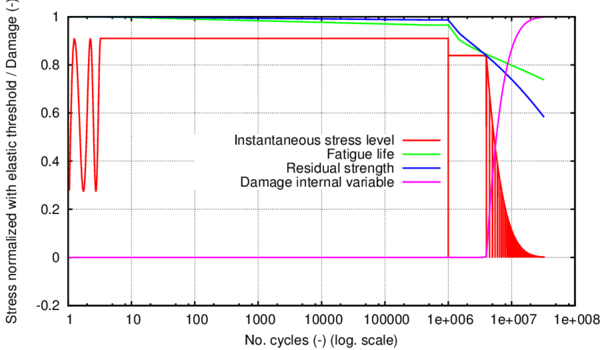
|
| Figure 68: Parameters of interest for the fatigue analysis under loads + |
Figure 69 shows the stress – strain curve where the stiffness reduction can be seen at each automatic unloading. The vertical axis refers to the instantaneous stress divided by the elastic limit. The trigger for the load-tracking stage is in an increment i. When this happens, the load factor for increment i+1 will be correspondent to the load-tracking phase and unloading will have begun. Each cycle will be described by small increments until the stress state is stable again from one cycle to the other. The curve is in accordance with figure 68, showing that the material is in the elastic state while load is applied and the equivalent stress is taken to its maximum value: 0.91 of the elastic limit. Load is then applied and takes the material to its fatigue life as indicated by the dynamically updated Wöhler curve. All the stiffness reduction occurs after this point. As seen in the previous case, a higher stiffness reduction can be seen in the first stages of the nonlinear process. Each one of the vertical segments depicting stress relaxation in figure 69 corresponds to a large increments phase that occurs only when . The inclined lines mark the posterior load-tracking phase with material loading-unloading.
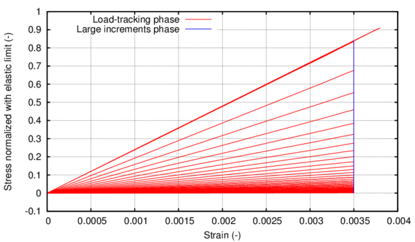
|
| Figure 69: Stress-Strain at integration point for loads + |
Another case is shown in figures 70 and 71 where the order of the loads is inverted. First, 10 cycles of load are applied, with its consequent strength reduction. After that, the load changes to and, in the first cycle it is applied, the maximum stress induced in the material is higher than the updated fatigue life curve. However, the updated material strength is above this value and the damage threshold in the constitutive model will not be crossed yet. When the stress state stabilizes under load a large increment is applied, and, due to this change in , the strength threshold is reduced below the maximum stress level material and the damage accumulation process starts. The switch is made back and forth between load-tracking and large increments until all the fracture energy of the material is dissipated.
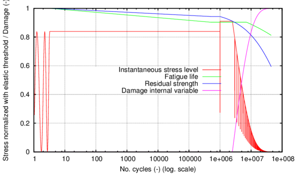
|
| Figure 70: Parameters of interest for the fatigue analysis under loads + |
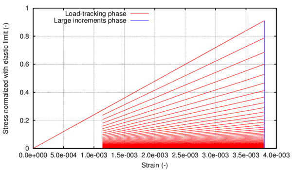
|
| Figure 71: Stress-Strain at integration point for loads + |
4.4.4 Load history with cyclic and monotonic loads
Following, several loading scenarios have been analysed that include a cyclical load and a monotonic one. A comparison is made between the material behaviour when failure occurs due to monotonic loading exclusively, due to cyclic loading exclusively or due to combinations of the two. Specifically, in the first case analysed the cyclic loading is applied 10 cycles and then the material is taken to complete failure by monotonic loading. In the second case the same cyclic load is maintained 6,42 x 10 cycles and a monotonic load is applied after that, until total failure.
The constitutive model quantifies the energy dissipation only after the curve has been crossed and the updated damage threshold surpassed. A question is raised then on whether dissipation occurs also before this point, in the span of when the initial elastic limit starts to be reduced, but the damage threshold has not been crossed yet.
This reduction in strength corresponds, from a physical point of view, to a rearrangement of the internal structure of the material, slip of metal grains and potential nucleation of voids. The dissipative cost of this process can be quantified indirectly by comparing the behaviour of the material taken to failure by a monotonic load, by a cyclical load and by different combinations of the two.
As said before, four different cases have been analysed, as shown in table 14. A different visual representation of the results has been chosen for these combinations in order to better differentiate cyclic from monotonic effects in a more graphical way.
| Case no. | Type of load | applied |
| 1 | cyclic + monotonic | 10 |
| 2 | cyclic + monotonic | 6.42 x 10 |
| 3 | cyclic | 34 x 10 |
| 4 | monotonic | 0 |
Figures 72, 73 and 74 show the parameters of interest for the fatigue damage model in a three-dimensional space. In the following, the X axis refers to the number of cycles axis where a logarithmical scale is used. On the Y axis the damage internal variable is portrayed, and in the Z axis the stress is quantified, scaled with the value of the initial elastic limit. While damage accumulation has not started, the curves of interest are contained in the XZ plane, same as the plots shown in previous cases. However, when the damage threshold is crossed the stress curve is taken outside of this plane by representing its evolution with the help of the Y axis where the damage variable is quantified.
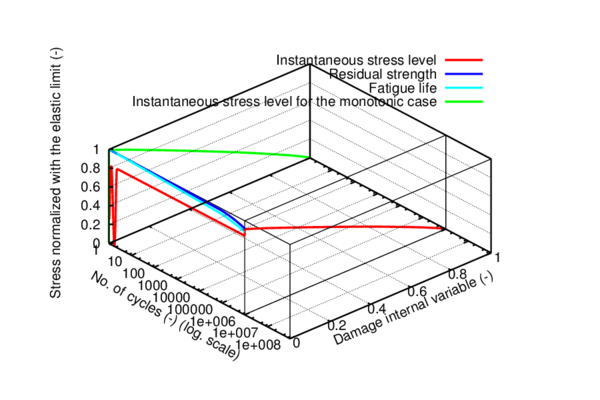
|
| Figure 72: Parameters of interest for the fatigue analysis under load combination 1 in 3d representation |
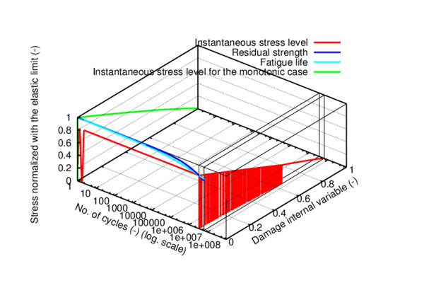
|
| Figure 73: Parameters of interest for the fatigue analysis under load combination 2 in 3d representation |

|
| Figure 74: Parameters of interest for the fatigue analysis under load in 3d representation |
Put in different words, all the YZ planes perpendicular to the fatigue curves in plane XZ show the dissipation for a monotonic loading applied at the where the plane intersects the X axis.
For instance in figure 72 the curves of interest are shown for case 1 in table 14. While the cyclic load is being applied the variables of interest are found in the XZ plane, where the strength reduction and the fatigue life are depicted. After 10 cycles the cyclic load is stopped and is then increased monotonically until failure (). When the load starts to be applied monotonically the material is still in the elastic state, but its elastic limit has been reduced. Therefore, damage starts earlier than if the cyclic load would not have been applied. The entire evolution of the stress curve after damage initiates in the model is contained in the plane perpendicular to the axis. On the same chart, the evolution of the stress is plotted for the monotonic case (Case 4 in table 14). In order to be able to represent both curves on the same chart the monotonic stress curve has been plotted in the plane with an abscissa of , even though the load was exclusively monotonic.
The same variables are shown in figure 73 for case 2 in table 14 and in figure 74 for case 3 in table 14. All the figures include the evolution of the monotonic stress curve for reference. It can be seen that as damage starts to accumulate due to cyclic loading the stress curve is no longer contained in a YZ plane but rather it describes a curvilinear trajectory in space, as can be seen clearly for case 3 in figure 74. The intersection of this curvilinear trajectory with a given YZ plane marks the beginning of the dissipation if the load were monotonic after that given . An example of the above is figure 73 for case 2 in table 14 where after 6.42 x 10 cycles the load is increased monotonically until failure and the remaining energy is dissipated in the corresponding YZ plane (with an abscissa of 6.42 x 10 cycles).
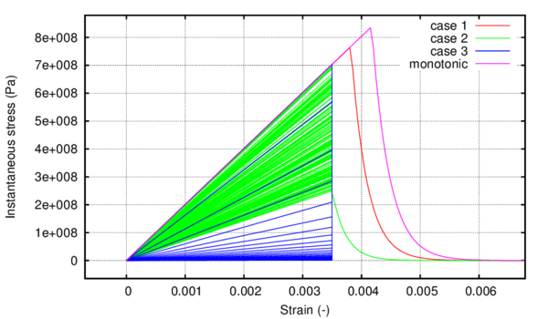
|
| Figure 75: Comparison between the stress-strain curves at the integration point for different load combinations |
In figure 75 the dissipative cost of the strength reduction occurring in the elastic zone can be seen by comparing the stress-strain curve for the monotonic case and for the other cases. The maximum energy dissipation cost (maximum area difference with respect to the monotonic curve) is visible for the case with only cyclic loading applied (case 3 in table 14).
For a final overview on the different stress histories used in this analysis, figure 76 can be consulted. The stress due to monotonic loads has been marked for each case analysed.
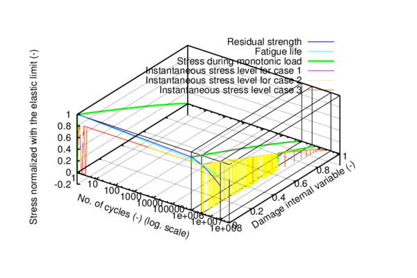
|
| Figure 76: Comparison between the stress evolution at the integration point for different load combinations in 3d representation |
4.5 Validation of the formulation proposed
4.5.1 Problem definition. Geometry and material.
The experiment undertaken by Marines et al. [131] has been chosen to validate the stepwise load advancing strategy presented in this work, together with the continuum damage model for fatigue described in section 4.2. In table 15, the material characteristics given by the aforementioned authors are presented along with the shape and dimensions of the fatigue specimen adopted in the experiment. The experimental results obtained with a loading frequency of 20 kHz and a reversion factor have been taken into account for the comparison with numerical results.
| E
(GPa) |
E
(GPa) |
(MPa) |
UTS
(MPa) |
A
(%) |
(kg/m) |
| 208.3 | 211.5 | 608 | 878 | 20 | 7850 |
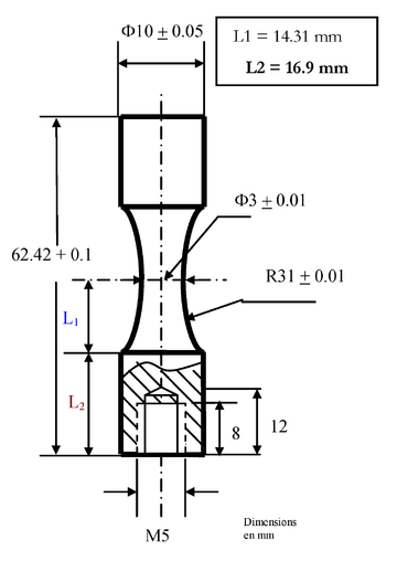 ] ]
|
| Figure 77: Shape and dimension of ultrasonic fatigue specimen as given by Marines et al.[131] |
4.5.2 Finite element model
The fatigue specimen presented in figure 77 has been reproduced by means of a finite element model. Due to the symmetrical nature of the geometry, loading and boundary conditions, only half of the specimen has been modelled in order to minimize computational time.
The semi-cylindrical volume has been meshed with linear hexahedral elements as shown in figure 78. The mesh has 2666 nodes and 1920 elements. Each finite element is described with eight integration points.
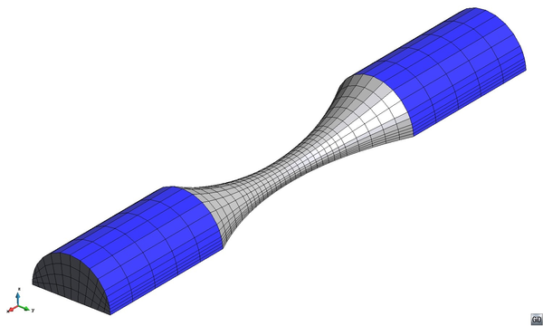
|
| Figure 78: Finite element mesh of linear hexahedral elements |
The boundary conditions applied are shown in figure 79. The specimen is restrained at one end and subjected to a cyclical displacement at the other end. The entire base is defined with a symmetry condition.
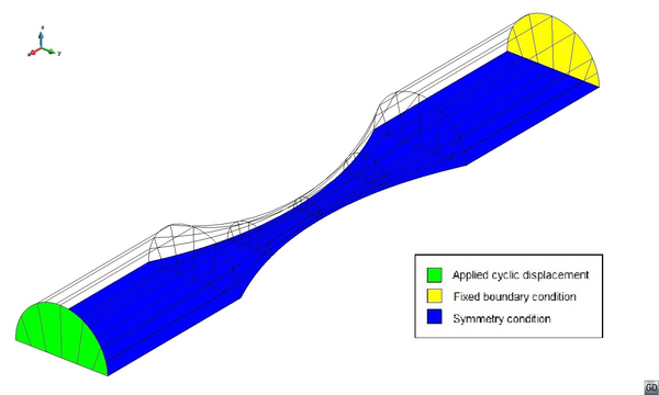
|
| Figure 79: Boundary and loading conditions for the analysed geometry |
The analytical formulation for the curve used by the numerical model was the one presented in [129]. The parameters used for the adjustment of the curve to the experimental one proposed by Marines et al. [131] are S= 608Mpa, S=325Mpa, = =1.3 a correction factor of 1.23 was applied when calculating the auxiliary term .
4.5.3 Results and discussion
In figure 80, the results obtained by Marines et al. [131] are presented. As expected, a scatter of test results can be seen both for 20 kHz resonating material and for the 30 kHz one. Since the material characteristics taken into account for the numerical analysis are that of the 20 kHz one, simulations have been run only with the maximum stress levels exhibited for this particular testing frequency. The experimental results showed that, even though the geometry and loading conditions are axisymmetric, the failure mode is not symmetric [131].
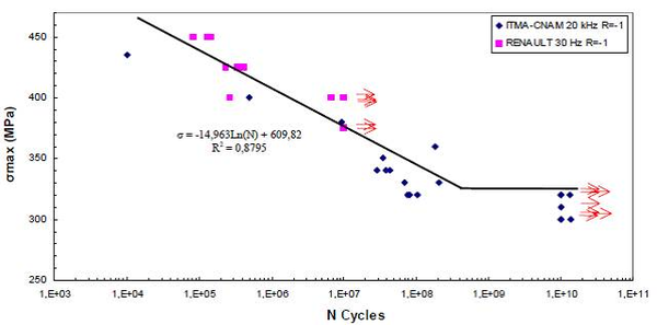 ] ]
|
| Figure 80: Fatigue S-N curve of HSLA steel D38MSV5S with R = -1, 20 kHz and 30kHz [131] |
4.5.3.1 Validation of the results obtained with the numerical simulation
The expression for the curve proposed in figure 80 by Marines et al. [131] has been compared to the numerical results obtained from the described finite element model. The comparison can be seen in figure 81. Since the model has a deterministic nature, no scatter can be seen in numerical results. The numerical data depicted in figure 81 is in accordance with table 16 where the information on the exact characteristics of each simulation case is given.
| Case code | Reversion factor | Max. Stress GP (MPa) | Nc at which damage initiates |
| BA1 | -1 | 435 | 0,17 * 10 |
| BA2 | -1 | 400 | 1,50 * 10 |
| BA3 | -1 | 380 | 5,30 * 10 |
| BA4 | -1 | 360 | 20,03 * 10 |
| BA5 | -1 | 350 | 39,50 * 10 |
| BA6 | -1 | 340 | 78,50 * 10 |
| BA7 | -1 | 330 | 160,00 * 10 |
| BA8 | -1 | 320 | 1E9 (run-out) |
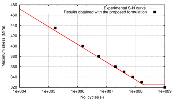
|
| Figure 81: curve for HSLA steel D38MSV5S. Experimental vs. numerical. |
Some observations are to be made, however, in order to better understand the results presented in figure 81. The points signalled as results obtained with the proposed formulation, mark the start of the stiffness reduction. In a force controlled test, when the force level is taken to the following maximum after the fatigue life depicted in figure 81, abrupt failure occurs. However, as the numerical model has been defined with displacement controlled boundary conditions, when the next maximum displacement is reached after arriving at the fatigue life given in table 16, a reduction of the stress level occurs and the material can continue to be cyclically loaded. If an unloading would be made at this point a stiffness reduction in proportion to the stress relaxation would be observed. For a better understanding of this effect a detailed description of the fatigue behaviour is shown in the next section for one of the cases ran for the validation.
Summarizing, the fatigue life charted in figure 81 represents the number of cycles up until which the maximum stress induced by the applied cyclical displacement remains unaltered. Once this point is surpassed, stress relaxation occurs along with damage accumulation, stiffness reduction and a subsequent change in internal forces. If the test is force controlled, the specimen fractures abruptly. If the test is displacement controlled, the material is taken to complete fracture progressively.
4.5.3.2 Analysis of the performance of the material model. In-depth analysis of stiffness reduction at integration point
In this section an in-depth analysis of the behaviour of the material is made for a maximum induced stress level of 350 MPa. The results are similar for all the other simulations ran.
The experimental tests have shown that fracture initiates on the surface of the specimen. This is due to defects present in the microstructure that lead to void nucleation and microcrack initiation and propagation. Fracture initiation is not symmetric and, furthermore, in the last stages of the nonlinear process, due to microstructural imperfections and defects, fracture propagation leads to non-symmetrical behaviour.
In the numerical simulation, same as in the experiment, fracture initiation is not symmetrical, but a large part of the propagation process occurs under symmetry to the y-y axis. However, in the last stages, before complete rupture (third image in figure 84), due to numerical round off the solution loses symmetry.
A monitoring of model parameters has been made at the first integration point that shows complete degradation. In figure 82 are depicted: the evolution of the residual strength, Wöhler fatigue life, equivalent stress and damage internal variable with a logarithmical scale along the horizontal axis. It can be seen that the stress state suffers no alteration until it intersects the curve, same as in the numerical examples shown so far.
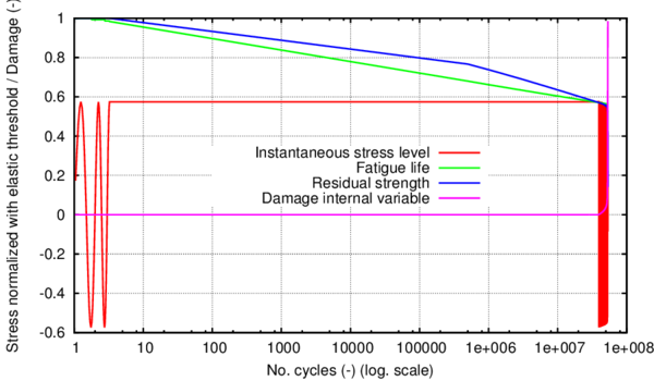
|
| Figure 82: Parameters of interest for the fatigue analysis of D38MSV5S specimen at the first integration point that fractures completely |
Figure 83 shows a zoom on the evolution of the variables in the non-linear zone (past the intersection with the curve). Here the succession between the large increments phase and the load-tracking phase can be better seen. Also, it can be observed how 90% of the degradation is concentrated in the last two large steps with nearly 80% in the last one. For this case, 0.5 x 10 cycles has been adopted as step for the large increments phase. Therefore, although the specimen is subjected to approximately 53.5 x 10 cycles until it fractures completely, 80% of the stiffness reduction occurs in the last 500000 cycles, deeming the fracture a "brittle" type one.
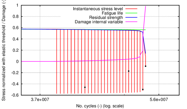
|
| Figure 83: Zoom on fatigue parameters of interest in the nonlinear zone (post curve).Dots indicate the analysis steps at which damage evolution is presented in figure 84 |
Figure 84 shows a view of the specimen from above and a view of the cross section at different number of cycles (analysis steps). Each one of the steps represented is marked in figure 83 chronologically with a black dot.
The images show the damage evolution in the specimen, both on the surface and in depth, as the number of cycles increases. Damage initiates on the surface of the specimen in the area with the smallest cross-sectional diameter, as expected, after 39.5 x 10 cycles. Afterwards it propagates symmetrically until approximately 53 x 10 cycles (third image in figure 84), when it localizes in one side of the specimen. This is believed to be due to a numerical round off that directs the posterior damage accumulation to the right side of the specimen, as can be seen in figure 84.
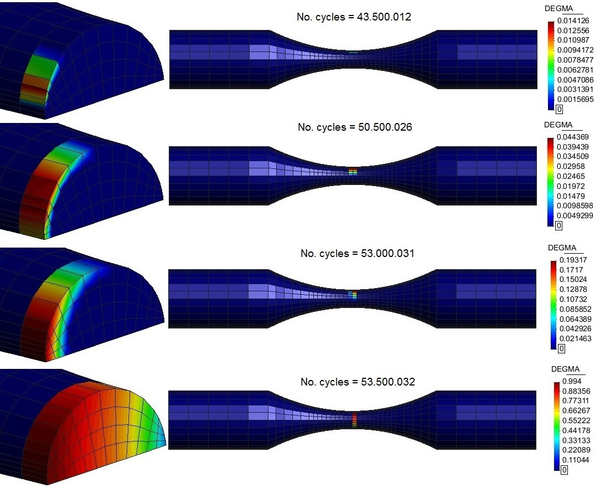
|
| Figure 84: Damage evolution for a maximum induced stress of 350MPa and R = -1 |
The upper image in figure 85 presents the deformed shape of the specimen when the last maximum displacement before total fracture is applied. A necking can be seen in the central region although the specimen is not yet completely fractured. From that point in the analysis, the applied displacement is taken from its maximum value to its minimum one, when the specimen is subjected to compression. That eventually causes the rupture into two parts (lower image in figure 85).
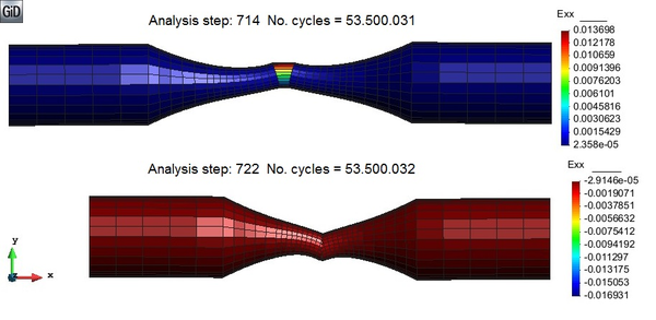
|
| Figure 85: Deformed shape (x 200) at the last maximum stress before rupture and at the last minimum stress, when rupture occurs |
5 Constitutive modelling of Low Cycle Fatigue
This chapter presents a coupled plastic damage constitutive model valid for materials subjected to LCF. The model is applied in the softening regime leading to an improvement in material life prediction as compared to plasticity models. The energy participation factors for damage and plasticity are dependent on the number of cycles of loading the material has been previously subjected to. Numerical examples are presented to illustrate the behaviour and capabilities of the model in softening behaviour under monotonic load, and hardening - softening behaviour under cyclic load incorporating both kinematic and isotropic hardening.
5.1 Introduction
Natural hazards, such as earthquakes and landslides, have in most cases a devastating impact on civil infrastructures, as they lead to important material and economic loses. Among the elements most affected are pipelines and pipeline systems (water, oil, gas, etc.), that can be substantially damaged, and whose reparation cost can be extremely large. For example, according to the data reported by Kimishima et al. [132] , the number of water pipes that broke during the 2007 Niigata-Ken Chuetsu-Oki earthquake exceeded 550.
Under seismic loads pipelines suffer large cyclic deformations that can lead to their failure or that can undermine their strength capacity for their future use. In these cases, material failure is frequently driven by Low and Ultra-Low Cycle Fatigue phenomena (LCF and ULCF, respectively). Thus, in order to minimize the effect of these loads on pipelines and pipeline systems, and to assess the vulnerability of existing infrastructures, it is necessary to have appropriate analysis tools to simulate the failure mode of steel under ULCF and LCF.
Current work presents a new constitutive model especially developed for the prediction of material failure produced by LCF and ULCF. The agreement obtained between experimental and numerical results allow considering the proposed law an excellent tool for the simulation of pipelines under seismic conditions, as it allows predicting the strength capacity of a pipeline under any given seismic load or assessing the residual strength of the pipeline once the seismic load has already been applied.
Material failure due to LCF and ULCF will be simulated using a material non-linear model. This approach will allow the simulation of regular and non-regular cycles, as well as obtaining the post-critical response of the structure when the material has failed.
A material non-linear model is defined by the thermodynamic law that drives the material performance and a yield criterion defining the stress level that triggers the non-linear behaviour ([92], [98]). The constitutive law proposed herein is characterized by the combination of plasticity and damage. These two material laws have been already coupled by several authors proposing different models. These models vary in their complexity, versatility and accuracy. Some of them are those of Simo and Ju [126], Lubliner et al. [82], Luccioni et al. [89] and, more recently, Armero and Oller [133].
The necessity of combining these two laws is based on the following assumption: The plastic phenomenon leads to the distortion of metal voids and their coalescence. This effect is responsible of the permanent deformations obtained after steel yielding, characteristic of plasticity. However, this process does not account for the formation or nucleation of new voids, which may reduce the material stiffness [134]. In order to include this effect in the material behaviour, a new law complementing plasticity is necessary. An increment of the voids in the microstructure of the material leads to a reduction of the effective area, resulting also in a reduction on the material stiffness. This effect will be simulated with a damage law.
The validity of this assumption is proved by a recent experimental campaign conducted in order to characterize the response of several steels for pipes (X52, X60 and X65) under ULCF and LCF loadings [101]. These tests showed that while the material is in the hardening region, its performance is fully defined by plasticity. This is proved by the fact that successive hysteresis loops lay one over the other. However, when the hysteresis loop shrinks due to material softening, the material also loses some stiffness, effect noticed in the change in slope of the stress-strain curve when unloading. This behaviour corresponds to damage.
Therefore, in order to predict accurately the response of pipe steel under ULCF and LCF loads, the model must couple plasticity and damage in different stages. Initially, the material hardening behaviour will be associated with plasticity. Afterwards, the material softening behaviour will be associated to both damage and plasticity. The evolution of plastic strains is taken into account by the plasticity model and at the same time the void formation and their subsequent coalescence is quantified phenomenologically by the damage model. Finally, failure will take place when all the fracture energy of the material has been dissipated.
The initial plastic model used for the hardening region of steel is the one decribed in chapter 3 of the current document and already published in [87] and [88]. This plasticity model is coupled with an isotropic damage model using the approach proposed in the work of Luccioni et al. [89] for monotonic loads. The coupling of these two models is made measuring, in every hysteresis cycle, the internal energy required by each model, as well as the available remaining energy of the material [135].
In the following section the formulation resulting from coupling the plasticity with the damage model is described in detail. Afterwards, section 5.3 presents the procedure defined to simulate LCF with the proposed constitutive law. Finally, section 5.4 compares the numerical results obtained with the proposed formulation with those obtained from the experimental campaign conducted by [101].
5.2 Plastic damage model formulation
5.2.1 Elasto-plastic damage model. Mechanical formulation.
The theories of plasticity and/or damage can simulate the material behaviour beyond the elastic range, taking into account the change in the strength of the material through the movement of the yield and/or damage surface (isotropic and kinematic) due to the inelastic behaviour (plasticity and damage) of each point of the solid. However they are not sensitive to cyclic load effects. In this work the standard inelastic theories are modified to introduce the fatigue effect coupled with non-fatigue material behaviour.
It is assumed that each point of the solid follows a damage-elasto-plastic constitutive law (stiffness hardening/softening) ([89], [82] and [136]) with the stress evolution depending on the free strain variable and plastic and damage internal variables. The formulation proposed herein studies the phenomenon of stiffness degradation and irreversible strain accumulation through the combined effect of damage and plasticity.
Since this work is oriented towards mechanical problems with small elastic strains and large inelastic strains, the free energy additively hypothesis is accepted ([92][91]). The elastic and plastic parts of the free energy are written in the reference configuration for elastic Green strains ; the last variable operates as a free field variable [126], [2]. The free energy is thus written as
|
|
(51) |
Considering the second thermodynamic law (Clausius-Duhem inequality – [91], [94] and [95]), the mechanical dissipation can be obtained as [92]:
|
|
(52) |
The fulfilment of this dissipation condition (Equation 52) demands that the expression of the stress should be defined as (Coleman method; see [95])
|
|
(53) |
Also, from the last expressions, the secant constitutive tensor can be obtained as:
|
|
(54) |
where is the material density, are the elastic, total and plastic strain tensors, is the internal damage variable enclosed between its initial value and its maximum value 1, is a plastic internal variable, and are the original and secant constitutive tensors and is the stress tensor for a single material point.
5.2.2 Yield and potential plastic functions
The yield function accounts for the residual strength of the material, which depends on the current stress state and the plastic internal variables and, in the formulation proposed herein, it is sensitive to the fatigue phenomenon. This function has the following form, taking into account isotropic and kinematic plastic hardening (Bauschinger effect [28]):
|
|
(55) |
where is the uniaxial equivalent stress function depending of the current value of the stresses , is the kinematic plastic hardening internal variable, is the plastic strength threshold and is the plastic isotropic hardening internal variable ([89], [82], and [136]). is the number of cycles of the stress in the point of the solid and is a symbolic notation for all the plastic variables involved in the process.
Equation 55 incorporates the number of cycles as an internal variable that affects the strength threshold by lowering it as the number of cycles accumulates. This enables the model to also account for strength reduction due to high cycle fatigue effects ([2], [103] and [104]) and this in turn shows the potential of the formulation to adjust by itself to the type of fatigue involved.
The evolution law for the plastic strain is , being the consistency plastic factor and the plastic potential.
Kinematic hardening accounts for a translation of the yield function and allows the representation of the Bauschinger effect in the case of cyclic loading. This translation is driven by the kinematic hardening internal variable which, in a general case, varies proportionally to the plastic strain of the material point. One of the laws that define the evolution of this parameter is
|
|
(56) |
where is a material property to be determined by particular tests for the Prager and Melan kinematic hardening [92]. The evolution of isotropic hardening is controlled by the evolution of the plastic hardening function , which is often defined by an internal variable . The rate equation for these two functions may be defined, respectively, by
|
|
(57) |
where denotes scalar and stands for a tensor function. Depending on the functions defined to characterize these two parameters, different solid performances are obtained.
5.2.3 Threshold damage function
Onset of damage depends on the current stress state, the internal damage variable and, with the current formulation, it also depends on the number of cycles. The threshold damage function is defined as (see [95] and [126])
|
|
(58) |
where is the equivalent stress function in the undamaged space, the damage strength threshold is , and the damage internal variable.
The evolution of the damage strength threshold is analogous to that of the plastic strength threshold, depending on the internal degradation variable
|
|
(59) |
In equation 59, is a scalar function with scalar arguments and is a scalar function with tensorial arguments as shown by [89], [87], and [135].
5.2.4 Coupled plastic-damaged response and tangent constitutive law
From the simultaneous consistency conditions for the plastic () and damage () problems, the evolution of the plastic strain and damage variables can be obtained. The secant constitutive law and the stress rate are
|
|
(60) |
|
|
(61) |
|
|
(62) |
Considering the stress rate as , the analytical expression of the tangent constitutive tensor is
|
|
(63) |
5.2.5 Algorithm for the numerical implementation of the plastic-damaged model
For this model, plasticity and damage equation must be integrated simultaneously. This is done with the following Euler-backward algorithm. Between two-equilibrium configurations and the formulation is updated as follows:
|
|
(64) |
|
|
(65) |
|
|
(66) |
|
|
(67) |
The stress state is updated according to the secant constitutive law shown in equation 61 and its reduction to the damage and plastic yield surfaces is done simultaneously, leading to the following non-linear system of equations:
|
|
(68) |
|
|
(69) |
This system of equations can be solved by the Newton-Raphson procedure [137]
|
|
(70) |
Despite having the analytical expression of the tangent constitutive tensor, equation 63, the calculation of this tensor is extremely costly and, depending on the yield and damage functions used, its approximation does not provide correct results. To overcome this drawback this tensor is calculated numerically by a perturbation method. This is obtained as
|
|
(71) |
with an infinitesimal perturbation applied to the mechanical strain tensor, and the stress variation produced by the strain perturbation. With this procedure, it is necessary to apply twice ab perturbations to obtain the complete tangent tensor. However, despite the computational cost, it provides an accurate approximation that improves the global convergence of the problem [99].
5.3 Plastic damage model oriented to fatigue analysis
The effects of a cyclic load on the constitutive behaviour of a material range from the accumulation of plastic strain in the case of ULCF to the reduction of material stiffness when dealing with high cycle fatigue. LCF induces changes in the material that are a combination of the aforementioned phenomena. In the following the methodology and motivation for taking into account the effects generated by the cyclical load will be presented.
5.3.1 Ultra-low cycle fatigue
The model is able to account for ULCF effects by incorporating a new law, especially developed for steel structures, that has been designed to reproduce their hardening and softening performance under monotonic and cyclic loading conditions (figure 86). This law depends on the fracture energy of the material.
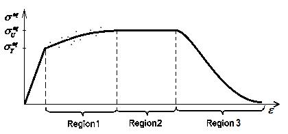
|
| Figure 86: Evolution of the equivalent stress |
The equivalent stress state shown in figure 86 has been defined to match the uniaxial stress evolution shown by most metallic materials. This curve is divided in two different regions. The first region is defined by fitting a curve to a given set of equivalent stress-equivalent strain points. This curve is a polynomial of any given order and is fitted by using the least squares method. The data given to define this region is expected to provide an increasing function, in order to obtain a good performance of the formulation for cyclic analysis.
The second region is defined with an exponential function to simulate softening. The function starts with a null slope that becomes negative as the equivalent plastic strains increase. The exact geometry of this last region depends on the fracture energy of the material. The exact formulation of the constitutive law can be found in Martinez et al. [87],[135] and has been presented in detail in chapter 3.
Characteristic of this type of fatigue is the Bauschinger effect that is taken into account in the constitutive model by combining isotropic hardening with kinematic hardening. The energy dissipated in each hysteresis loop is monitored and failure under cyclical loads is reached when the total available fracture energy of the material is spent.
The plastic damage formulation presented in this paper can be used to improve result accuracy when simulating the softening behaviour under ULCF loads.
5.3.2 Low cycle fatigue
The behaviour of a material subjected to cyclical loads that induce LCF exhibits both accumulation of plastic strain and a reduction of stiffness (Figure 87). While ULCF can be described exclusively by plastic models and HCF by damage models, LCF should be modelled with coupled plastic damage models. It is often difficult to predict at which moment in the material life the stiffness reduction begins, since the boundaries between these types of fatigue are rather arbitrary. Stiffness reduction is understood as the change in slope when unloading occurs in a cycle of loading, and is generally present only when softening has begun. The model this work proposes aims at making a contribution in correctly assessing the fatigue life for materials subjected to ULCF and LCF and is particularly effective for the transition zone between these two phenomena.
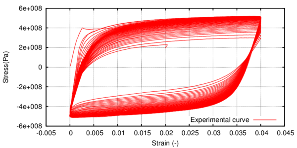 ] ]
|
| Figure 87: Experimental stress-strain curve for X52 steel [101] |
In the context of the hardening law proposed for ULCF, the plastic damage model presented in this work activates itself in the softening region. This is justified by the physical implications behind the damage phenomenon, as damage induces porosity that leads to stress relaxation. This implies that regions 1 and 2 in figure 86 are governed by plasticity ensuring that only the cyclical loads that last a long enough number of cycles get to experience damage effects. This is important as the formulation is meant to guarantee that, for a material life clearly in the ULCF range (dozens of cycles or less), the constitutive equations governing are those of plasticity. By regulating the extension of regions 1+2 with respect to region 3 discrimination is made between materials that exhibit more sensitivity to ULCF with respect to LCF or the opposite.
5.3.3 Energy distribution law
The hardening law proposed in figure 86 marks as the onset of softening, the level of equivalent plastic strain inputted by user [87]. This is the triggering point for the plastic damage model to activate itself. At this point the total energy dissipated by the plasticity model has been quantified and, by subtracting it from the total fracture energy of the material, the energy available for the plastic damage model is obtained.
This work proposes an energy distribution law that determines how much energy goes to the plasticity model and how much goes to the damage model. The following law is proposed in order to assess this issue, where is the number of cycles the material has been subjected to, up until the first increment when softening begins, is the limit between the ULCF domain and the LCF one and is the limit between the LCF domain and the HCF one (figure 88):
|
|
(72) |
The percentage of energy allocated to plasticity is the complementary part, . By multiplying these percentages to the energy available for the softening process, , the nominal energy for each process is obtained: and .
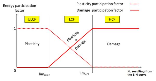
|
| Figure 88: Schematic representation of the energy distribution law in softening over the entire fatigue domain (X axis not scaled) |
If at the onset of softening the number of cycles recorded is lower than the , then the and , thus marking the behaviour as completely governed by plasticity. When the number of cycles is greater than the limit between LCF and HCF then the entire energy available for the softening part goes to damage.
Although the energy distribution law is formulated in a straightforward and simple manner, the main difficulty lies in correctly assessing the number of cycles considered as a limit in between ULCF and LCF, and LCF and HCF. These limits can be derived statistically if an experimental program is available for small scale specimens. The statistical analysis has to be made taking into account the loading cycle when softening begins.
These limits are material dependent, as each material exhibits a different behaviour in terms of the vulnerability to ULCF or HCF conditions. Consider for instance two materials that exhibit the same total fatigue life (hardening + softening) for a certain straining amplitude, but have different onsets for the softening process. The stress-strain hysteresis loop for the entire load history is different and a more accurate monitoring of the exact onset of softening leads to a finer tuning in terms of strain based design.
5.4 Performance of the formulation
In the following the results obtained for several simulations, conducted to illustrate the performance of the formulation presented, are included. These simulations prove the ability of the formulation to characterize mechanical softening behaviour, under monotonic and cyclic loading conditions. The main aim of all these simulations is to show the response obtained with the proposed constitutive model. Therefore, for the sake of simplicity, and to reduce the computational cost of the simulations, all of them have been conducted on a single hexahedral finite element. The element is fixed in one of its faces and the load is applied to the opposite face as an imposed displacement.
5.4.1 Mechanical performance under monotonic loads with softening constitutive behaviour
The first simulation presents the capabilities of the formulation when dealing with materials that exhibit softening behaviour. The material characteristics are given in table 17 and belong to a hypothetic material.
| Young Modulus | 2.01 * 10 | MPa |
| Poisson Ratio | 0.30 | |
| Yield Stress () | 838.9 | MPa |
| Fracture Energy | 0.1 | MN * m/m |
Figure 89 shows the evolution of the stress for the plastic damage model as compared with the same simulation conducted with a classic plasticity model and with a classical scalar damage model such as that proposed by Kachanov [33].
Three different simulations were made with the coupled model. The first one assumes equal distribution of energy between the two interconnected phenomena: 50% for damage and 50% for plasticity. A different one was made with 10% for damage and 90% for plasticity and the last one allotted 90% for damage and 10% for plasticity. Unloading was made at approximately the middle of the loading history in order to observe better the material behaviour. For the numerical simulations using the two uncoupled models, the entire available fracture energy was used (100%
It can be seen in figure 89 that, unless the material is unloaded, the behaviour is the same in all the simulations ran. When unloading, the loss of stiffness and the accumulated plastic strain are in accordance with the percentage of energy given to each one of the models. For instance, for the simulation performed with 50% of the energy in damage and 50% in plasticity, when the material is completely unloaded the plastic strain corresponding to the coupled model is 50% of the plastic strain of the uncoupled plastic model. Also, the stiffness reduction is only 50% of the stiffness loss corresponding to the uncoupled damage model.
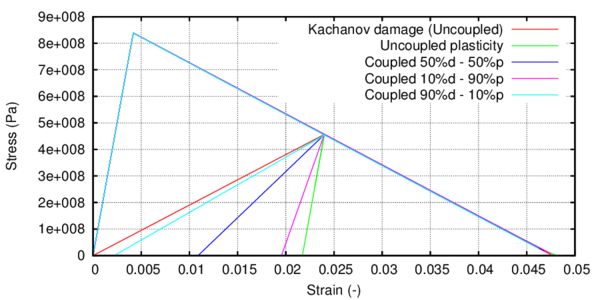
|
| Figure 89: Stress evolution for the plastic damage model as compared to the classical plasticity and damage models |
Both internal variables of the model, and , reach a unitary value at the end of the simulation. This states that the energy available for each process has been spent and that, on the whole, all the available internal energy of the material has been dissipated
|
|
(73) |
where p% is the participation factor for the damage process.
5.4.2 Mechanical performance under cyclic loads with hardening - softening constitutive behaviour
In this section, the material behaviour will be simulated with the hardening-softening law described in [87] and [135]. Both kinematic and isotropic hardening is taken into account. The hardening region will make use of the plasticity formulation described in chapter 3, while the softening region will be described with the plastic damage formulation presented in this chapter. The transition from one constitutive formulation to the other is done automatically at the material points that have reached softening. In table 18 the material properties used for this simulation are presented. An X60 steel has been used as material for this simulation. The experimental behaviour presented below is obtained from an experimental campaign conducted on smooth specimens by FEUP under the framework of the ULCF European Project "Ultra low cycle fatigue of steel under cyclic high-strain loading conditions. The properties displayed in table 18 have been obtained as result of a calibration analysis with the above mentioned experimental campaign.
| Young Modulus | 1.95 * 10 | MPa |
| Poisson Ratio | 0.30 | |
| Yield Stress () | 380 | MPa |
| Plastic Strain Softening () | 50 | % |
| C1 kinematic hardening | 6.0 * 10 | MPa |
| C2 kinematic hardening | 400 | |
| Fracture Energy | 15.0 | MN * m/m |
The fracture energy available for the coupled model is inherited as output from the plastic model. The input is the total available fracture energy along with all the other characteristics of the material, kinematic coefficients and the equivalent plastic deformation at which softening starts in the uniaxial experimental stress-strain curve. The model is highly sensible to the fracture energy available to the damage model.
For this simulation, the Friederick – Armstrong non-linear kinematic hardening was used. The limit between ULCF- LCF was chosen statistically from the experimental program made by Pereira et al. [101] as cycles. The limit between LCF and HCF was chosen empirically as 10 cycles.
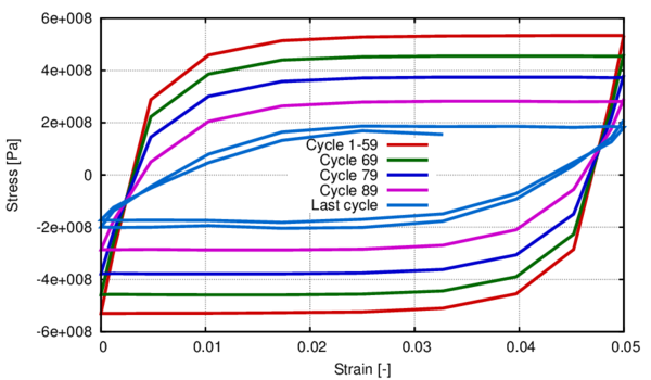
|
| Figure 90: Stress – strain curve obtained with the plastic damage model |
Figure 90 shows the stress-strain curve for a cyclic load with strain amplitude of 5% and a reversion factor equal to 0, when using the proposed plastic damage model in softening. Using the energy distribution law proposed in section 5.3.3, the participation factor for the damage process was of the fracture energy available for the softening stage. The evolution of the stress-strain curve has been plotted at every 10 cycles after softening has begun, in order for the progressive loss of stiffness to be better seen.
In figure 91 the evolution of the internal variables of the model can be seen. The vertical axis is scaled from 0 to 1 both for the damage internal variable and for the plastic internal variable. The meaning of this plastic internal variable is that of the plastic dissipation divided by the fracture energy available for plasticity. It can be seen that the damage process is activated at the beginning of softening (60 cycle). At this point, the integration scheme changes to simultaneous integration of both damage and plasticity equations. From the total facture energy of the material the part spent in hardening is subtracted and the remaining quantity is split between damage and plasticity using the law presented in section 5.3.3.
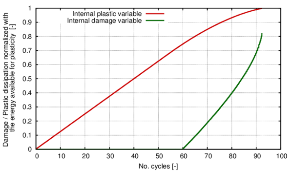
|
| Figure 91: Evolution of the internal variables of the plastic damage model |
In figures 92 - 96 a series of five snapshots are shown that compare the experimental stress-strain result with the numerical simulations made with the plasticity model and with the plastic damage model. In both simulations softening initiates in the 60 cycle, with a total life of 90 cycles for the first simulation and 93 cycles for the second one.
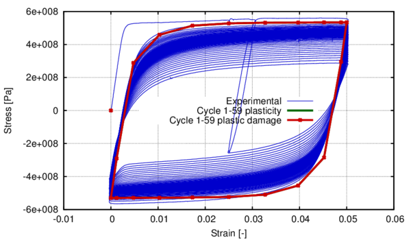
|
| Figure 92: Evolution of the stress- strain curve. Comparison between the experimental behavior and the numerical one when using plasticity equations and plastic damage equations at cycles 1-59 |
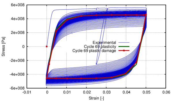
|
| Figure 93: Evolution of the stress- strain curve at cycle 69 |
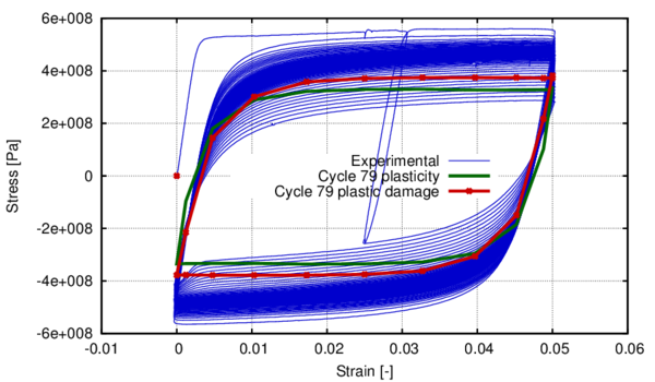
|
| Figure 94: Evolution of the stress- strain curve at cycle 79 |
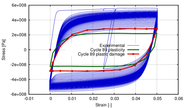
|
| Figure 95: Evolution of the stress- strain curve at cycle 89 |
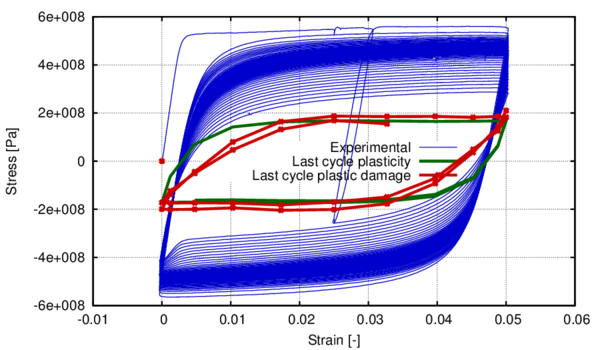
|
| Figure 96: Evolution of the stress- strain curve at the last cycle of the numerical simulation |
Several observations can be made when analysing figures 92 - 96.
First, a progressive reduction in stiffness can be observed from cycle to cycle when the proposed model is used, that allows a more accurate representation of the experimental behaviour than if only plasticity is taken onto account. Therefore, it can be said that the hysteresis obtained in softening with the plastic damage model is closer to the experimental behaviour.
Second, for the same moment in load history, the maximum stress decreases less when using the plastic damage model than if only using plasticity equations. Again, this is a result that indicates that the plastic damage model is closer to the experimental behaviour.
Third, when considering the final cycles of the analysis (figures 95 and 96), it can be seen that the stress does not decrease to 0 despite the fact that the internal energy of the material has been totally spent. This behaviour is displayed both in the numerical model and in the experiment, but the two numerical models seem to totally exhaust the load baring capacity of the material at a lower level of stress than the experimental result. This residual stress is a consequence of the kinematic hardening and the results obtained with the two numerical simulations suggest that, for this particular cyclic load, a lower elastic limit and higher kinematic coefficients would have better approximated the hysteresis and residual stress at the end of the simulation.
6 Extension of the High Cycle Fatigue model to composites
This chapter presents the methodology of application of the HCF damage model to composite materials. The composite behaviour will be obtained by means of the serial/parallel mixing theory that is also used as a constitutive equation manager. This formulation is based on the composition of the fatigue behaviour of each component and interface. The constitutive formulation is coupled with the load advancing strategy in order to reduce the computational cost of the numerical simulations. Validation of the constitutive formulation is done on pultruded glass fiber reinforced polymer profiles. Special emphasis is made on the comparison between the experimental and the numerical failure mode.
6.1 Introduction
The chosen approach in the present work is a phenomenological strength reduction model at constituent constitutive level based on the formulation adopted for metals under cyclic loading condition [2],[104]. The stresses and strains of the composite constituents are calculated using the serial/parallel mixing theory (SP RoM) [74], which allows different constitutive behaviour for each of the composite components and can accurately model delamination effects which are expected to be a consequence of fatigue damage. This theory is based on the definition of some compatibility equations between the strain–stress states of the composite constituent materials. In the case of a composite made of fiber and matrix, what the Serial/Parallel mixing theory does is to impose an iso–strain condition on the parallel direction, usually the fiber direction, and an iso–stress condition on the serial direction, usually the remaining directions of the stress and strain tensors. With this scope, if the matrix structural capacity is lost, the Serial/Parallel mixing theory will reduce the structural capacity of fiber material in the serial directions due to the iso–stress condition. Thus, it will be impossible for the composite layer to develop shear or transversal stresses, less to transmit them to the surroundings elements. It has been already proved in Martinez et al. [100] that the structural failure just described is equivalent to a delamination failure.
The basis of the high cycle fatigue constitutive model has been described in chpater 4 of this document. The model establishes a relationship between the residual material strength and the damage threshold evolution, controlled by the material internal variables and by a new state variable of fatigue that incorporates the influence of the cyclic load.
This constitutive model has been developed for HCF in steel and included a load - advance strategy that allowed advancing by large loading steps. This work is focused in assessing its life prediction capability for HCF in composites while taking advantage of the load-advancing strategy. The formulation for the load advancing strategy is also provided in chapter 4.
The formulation this chapter presents is validated on pultruded glass fiber reinforced polymer profiles by comparing experimental values with the values obtained from a numerical simulation. The next section describes the serial/parallel mixing theory used, the SP RoM, and how it is implemented in a finite element code. The following section describes the test simulated. Finally, the results obtained from the simulation are studied and compared to the experimental ones.
6.2 Rule of mixtures
The serial/parallel mixing theory (SP RoM) is based on the definition of two different compatibility equations between the strain and stress states of the composite constituent materials: it defines an iso-strain condition on the parallel direction, usually the fiber direction, and it defines an iso-stress condition on the serial direction, usually the remaining directions. Using these compatibility equations in a composite made of matrix and fiber, if the matrix structural capacity is lost due to excessive shear stresses, the iso-stress condition also reduces the shear capacity of fiber, and consequently the composite serial strength is also reduced.
For this reason it is necessary to define, and split, the serial and parallel parts of the strain and stress tensors. This is done with two complementary fourth order projector tensors, one corresponding to the serial direction () and the other to the parallel direction (). These tensors are defined from the fiber axial direction in the composite. Thus,
|
|
(74) |
where,
|
|
(75) |
Being , the director vector that determines the parallel behaviour (fiber direction), and the identity. The stress state may be split analogously, finding its parallel and serial parts using also the 4th order tensors and :
|
|
(76) |
6.2.1 Hypothesis for the numerical modelling
The numerical model developed to take into account this strain-stress state is based on the following hypothesis:
1. The composite is composed by only two components: fiber and matrix.
2. Component materials have the same strain in parallel (fiber) direction.
3. Component materials have the same stress in serial direction.
4. Composite material response is in direct relation with the volume fractions of compounding materials.
5. Homogeneous distribution of phases is considered in the composite.
6. Perfect bounding between components is also considered.
6.2.2 Constitutive equations of component materials
Each composite component material is computed with its own constitutive equation. However, as in this work the materials will be modelled with a damage formulation, the description of the formulation is done considering the particular case of isotropic damage. So, the stresses in matrix and fiber materials are obtained using:
|
|
(77) |
being and the matrix and fiber stiffness tensors, respectively. These equations can be rewritten taking into account the serial and parallel split of strain and stress tensors (equations 74 and 76), obtaining:
|
|
(78) |
where
|
|
(79) |
6.2.3 Equilibrium and compatibility equations
The equations that define the stress equilibrium and establish the strain compatibility between components arise from the analysis of the hypotheses previously exposed,
|
|
(80) |
|
|
(81) |
where superscripts , and stand for composite, matrix and fiber, respectively, and corresponds to the volume fraction coefficient of each constituent in the composite.
6.2.4 Serial/parallel rule of mixtures algorithm
The known variable that enters the algorithm is the strain state of the composite material at time . From this variable, the serial/parallel rule of mixtures algorithm has to find the strain and stress state of each component that fulfils the equilibrium, the compatibility and the constitutive equations and the evolution of the internal variables. The first thing done by the algorithm is to split the strain tensor into its parallel and its serial parts, in order to compute the strain state in the matrix and the fiber. The parallel strain component is, according to equation 80, the same for both materials and for the composite. On the other hand, the serial strain component requires a prediction of the strains expected in one of the composite components. If this prediction is done for the matrix, the increment of its serial strains can be computed as
|
|
(82) |
with and .
The initial prediction of matrix serial strains, proposed by Rastellini [138] and described in equation 82, is obtained considering that the distribution of the total strain, in its parallel and serial parts, is done in function of the composite tangent stiffness obtained in previous time step. With the prediction of the matrix serial strains, the fiber serial strains can be computed, in the iteration step n, according to equation 81,
|
|
(83) |
where .
Regrouping again the serial and parallel components of the strain tensor (equation 76), the constitutive equations can be applied to the predicted strains to obtain the stress tensor for both materials and the update of their internal variables. fiber and matrix are modelled, each one, with their own constitutive law. If both materials are described with an additive plasticity formulation, the stress vector for each one is obtained using equation 77. The stresses obtained must fulfil the following equation:
|
|
(84) |
If the residual stress is smaller than the tolerance, the computed strains and stresses are considered to be correct and the structural calculation can continue. However, if equation 84 is not fulfilled, the initial prediction of the matrix strain tensor has to be corrected. This correction is performed using a Newton-Raphson scheme, in which the update is made using the Jacobian of the residual forces. It is obtained deriving the residue function with respect to the unknown. According to Rastellini [139], the expression for the Jacobian is given as follows:
|
|
(85) |
and, the correction of the matrix serial strains becomes
|
|
(86) |
To obtain quadratic convergence in the S/P mixing theory, the Jacobian must be obtained using the tangent constitutive tensors for the fibers and the matrix. Depending on the constitutive equation defined for each material, the constitutive tensor cannot be obtained analytically. Thus, in order to obtain a reliable algorithm, the expression of the tangent tensor is obtained numerically with the procedure shown in Martinez et al. [74], [100].
6.3 Numerical simulation of GFRP profile
The capabilities of the fatigue constitutive model, together with the stepwise load-advancing strategy presented, will be shown by comparing results obtained from numerical simulations with the results provided in the experimental work presented in Keller et al. [140] .
All the examples presented in this section have been calculated with the PLCd finite element code [102], where the formulation presented here has been implemented.
6.3.1 Problem definition. Geometry and material.
Pultruded GFRP plate profiles with 100 5 mm rectangular cross-section were examined. The plates consisted of E-glass fibers embedded in an isophthalic polyester resin. The fiber architecture comprised mainly unidirectional rovings in the central region and one combined mat in the outside regions [141]. The combined mats consisted of chopped strand mats (CSM) and woven mats 0/90 of different weights; these two mats were stitched together. Furthermore, a polyester surface veil (40 g/m2) was added. The corresponding experimental fiber fractions are listed in table 19. They were determined by weighing the specimen before and after a resin burn-off in a furnace at 450 C. The experimental volume fractions were calculated using an E-glass density of 2.56 g/cm3. Since the fatigue behaviour is influenced by internal material defects and voids, some cross-sections were investigated by means of microscopy. The analysis showed a very good embedment of the fibers without any voids [141].
| Architecture | % by volume | % by weight | |
| Rovings (UD) | 4:1 Straight and blown | 37 | 53 |
| Combined mats: | 2 1 | ||
| CSM (g/m) | 300 | 5 | 7 |
| woven 0/90 | 150/150 | 5 | 7 |
| Total | 47 | 67 |
The specimen shape used was a tapered form (TP specimens, dog-bone shape) presented in figure 97. They were cut with a water-jet into a dog-bone form according to ASTM E 466-96 with a gage length of 300 mm, a gage width of 40 mm and, accordingly, a grip-to-gage width ratio of 2.5. The radius of curvature between the ends was 390 mm. The TP specimens were left in a laboratory environment for more than one week prior to testing to reduce the moisture effects induced during the cutting process [140].
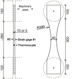 ] ]
|
| Figure 97: Experiment specimen with strain and temperature gages [140] |
6.3.2 Finite element model
The fatigue specimen presented in figure 97 has been reproduced by means of a finite element model. The dog-bone shape volume has been meshed with quadratic hexahedral elements as shown in figure 98. The mesh has 13896 nodes and 2354 elements. Each finite element is described with 27 integration points.

|
| Figure 98: Finite element mesh of quadratic hexahedral elements |
The boundary conditions applied are shown in figure 99. The specimen is restrained at one end and subjected to a cyclical displacement at the other end. All numerical simulations have been conducted under displacement-controlled conditions.

|
| Figure 99: Boundary and loading conditions for the analysed geometry |
The analytical formulation for the curve used by the numerical model was the one presented in [2] and shown in chapter 4. A decomposition of the experimental curve of the composite found in Keller et al. [140] has been made. The maximum composite stress for each experimental test has been decomposed according to the volumetric participation of each component into a maximum associated stress in the matrix and a maximum associated stress in the fiber. Using this decomposition associated points have resulted for the matrix and fiber as derived from the experimental composite curve. Afterwards, a calibration process has been conducted for both the fiber and the matrix in order to find the material parameters that approximate correctly those points. The parameters used for the adjustment of the numerical curve to the experimental one proposed by Keller et al. [140] are , , , , , and for the matrix and for the fiber , , , , , and .
The material properties used in the numerical simulations are shown in table 20.
| Component | Ultimate limit strength UTS (MPa) | E-Modulus longitudinal (GPa) | E-Modulus transversal (GPa) | Fracture energy (MN*m/m2) |
| Fiber | 2000 | 78.5 | 3 | 500 |
| Matrix | 75 | 3 | 3 | 10 |
6.3.3 Experimental program
The experiments were performed in a laboratory environment at room temperature without humidity control. Effects of environmental exposures (temperature, moisture, chemicals) on the fatigue behaviour were not investigated.
First, single-cycle axial tension experiments were performed with displacement-controlled loading at a rate of 0.6 mm/min up to failure. The numbers of experiments per specimen shape are listed in table 21.
| Specimen | Ultimate limit strength UTS (MPa) | Failure strain (%) | E-Modulus (MPa) |
| 5 mm tapered | 459 24 | 1.37 0.07 | 34,799 584 |
| (3 specimens) |
Subsequently, cyclic axial tension–tension experiments were conducted under load-controlled conditions with a sinusoidal waveform of constant amplitude. The specimens were loaded at a minimum to maximum load ratio of and at different loading ranges. The upper boundary values were varied from 20% up to 80% of the average ultimate tension strength (UTS) of the static experiments (see table 21). The used frequencies varied between 1 and 12 Hz. Due to practical reasons, the highest frequencies were used for the lowest loading ranges with maximum fatigue life and vice versa. Experiments were performed up to specimen failure (separation of samples) or up to ten million load cycles at maximum (if possible due to time constraints). The parameter combinations used in this study are summarized in table 22.
| Specimen | Loading range F (kN) | Stress range (MPa) | Maximum (ultimate) load (%) | Amplitude ratio R | Cycles to failure N | Remarks |
| TP5-1 | 65 | 325 | 82 | 0.13 | 1346 | |
| TP5-2 | 48 | 240 | 60 | 0.13 | 13,407 | |
| TP5-3 | 47 | 235 | 59 | 0.13 | 19,159 | |
| TP5-4 | 33 | 165 | 41 | 0.13 | 1,875,940 | |
| TP5-5 | 17 | 85 | 22 | 0.15 | 5,000,000 | not failed |
6.3.4 Results and discussion
The simulation program begun with a trial static simulation in order to confirm that the volumetric participations used in the numerical simulations yielded the same initial stiffness as the experimental results. The experimental stresses shown in table 21 were calculated from the measured loads (average stress in the cross-section); the strains were obtained from the average measurements from strain gages 1 and 2 (see figure 97). Due to the experimental fiber architecture of the specimen (detailed in table 19) the first combination of volumetric participations tested was 42% fibers and 58% matrix. These values have been chosen in order to approximate the contribution of the two combined mats consisting of chopped strand mats (CSM) and woven mats 0/90 of different weights. In the numerical simulation these mats were not specifically discretized as a different material. Therefore, by increasing the volumetric participation of the fibers with respect to the UD rovings, their effect was to be taken into account in a homogenized way. Even though the two combined mats increased the volumetric fiber participation by 10%, only a 5% increase has been considered numerically since it was considered that the longitudinal contribution of the mats were of only 5%, an assumption made by Keller et al. [140]. However, it can be seen from figure 100 that the initial stiffness obtained in the numerical simulation with this volumetric participation is not in accordance with the experimental recordings (14.65% error in strain for a stress level of 400MPa). The next fiber percentage tested was 37%, the percentage experimental recordings showed to correspond to the UD rovings. For this percentage the error was of only 3,76% for the same stress level and this was considered acceptable.
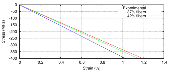
|
| Figure 100: Initial stiffness for the static case. Comparison between experimental and numerical values. |
Following, cyclic simulations have been ran with an applied displacement that induced the same stress amplitude and maximum stress as the experimental recordings in table 22. From these simulations two aspects are analysed in detail: the failure mode and the number of cycles until failure.
6.3.4.1 Failure mode
Some considerations have to be made with respect to the experimental failure mode. The static tests showed that the stress–strain relationship of the profiles was almost linear-elastic up to failure. Failure always occurred in a very brittle and sudden manner without any visible or audible signs (such as surface cracks or cracking noises). Therefore, it could not be determined where the fracture initiated. The specimens showed principally one diagonal crack in the tapered region and some small longitudinal cracks in the grip region (see figure 101) and they were split-up in the profile plane mainly between the outer layers containing the combined mats and the center part containing the UD-rovings. The length of the split parts spanned, more or less, the beginning and the end of the diagonal cracks and the whole profile widths. The center parts were split-up themselves along bundles of UD-rovings and resin. The diagonal cracks formed principally in the outer layers containing the combined mats. The fiber failures of the UD-rovings were distributed longitudinally in the split-up parts and were not concentrated in the diagonal cracks. All of the UD-roving fibers must have been failed within the split-up parts since no further load could be applied.
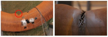
|
| Figure 101: Static (above) and fatigue (below) experimental failure modes |
During the fatigue tests, 4 specimens fractured while one specimen did not fail (see table 22). The failure modes under fatigue loadings were basically identical to the failure modes under quasi-static loadings. In several specimens, however, the widths of the cracks in the outer profile layers and the total elongations of the specimens were much more significant in the fatigue experiments compared to the static experiments. This observation can be explained by the progressive deterioration of the matrix and fiber/matrix interfaces, which led to easier pull out of the failed fibers [140].
The failure mode obtained in the numerical simulations can be seen in figure 102 for one of the numerical simulations. Specifically this simulation was set to run with the same characteristics as specimen TP5-1 in table 22. The diagonal distribution of the cracks was not found in any of the numerical simulations. A possible reason is that the combined mats where the diagonal experimental cracks were located were not taken into account in the numerical simulation.
In the numerical simulation the specimen lasted a total of 1311.08 cycles until failure. The distribution of the damage parameter for the composite material is shown at different time steps. It can be seen that damage initiates in the numerical simulation in the exterior parts of the curvature. As the number of cycles applied increases, the internal damage variable continues to increase in those same areas and consequently stress redistribution occurs in the material. This stress redistribution activates the central area of the specimen where damage starts to accumulate also, cutting thru the cross sectional area of the specimen, perpendicular to its longitudinal axis. It should be noted that in the numerical simulation the failure mode is symmetric. Damage propagation in the width of the specimen occurred mainly in the two last cycles of the simulation, indicating that the failure mode in the numerical model was also brittle, same as in the experiment.
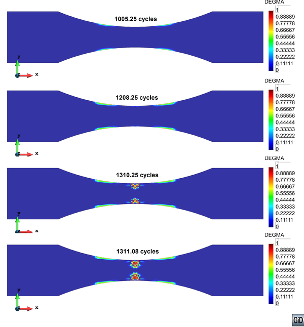
|
| Figure 102: Distribution of the damage internal variable for the composite at different time steps |
Figure 103 shows the evolution of the damage parameter in the glass fibers. It can be seen that while damage is located in the exterior area of the curvature the fibers remain in an elastic state. Only after approximately 1200 cycles the fibers in the central area of the model start to enter into the nonlinear domain due to the reduction in strength caused by the reduction coefficient, , propagating thru the width of the specimen mostly in the last two cycles of the simulation. In figure 104 it can be seen that damage in the external areas of the specimen curvature appears due to matrix degradation. However, only the matrix cracking is not enough to lead to specimen failure. Only when fiber degradation occurs failure is reached and this happens due to cross sectional degradation until the remaining area cannot bear the applied cyclic loading.
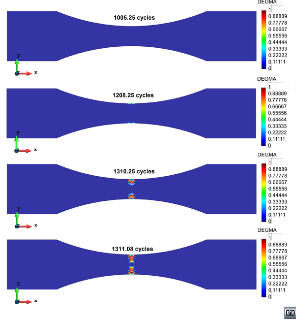
|
| Figure 103: Distribution of the damage parameter in the glass fibers at different time steps |
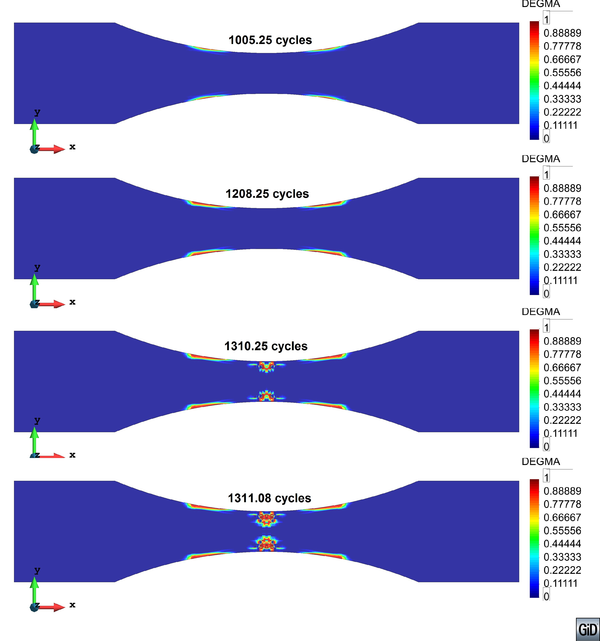
|
| Figure 104: Distribution of the damage parameter in the isophtalic matrix at different time steps |
In figure 105 a zoom on the central damaged area of the specimen is shown.
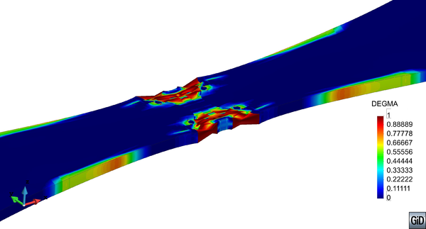
|
| Figure 105: Composite damage distribution in the last step of the analysis on the deformed specimen shape (20x) |
The distribution of the damage parameter for the composite material is painted on the deformed shape of the specimen, scaled 20 times. Again it can be observed that failure is caused due to damage in the central area, also visible when observing the longitudinal strain distribution in the last step of the analysis (figure 106).
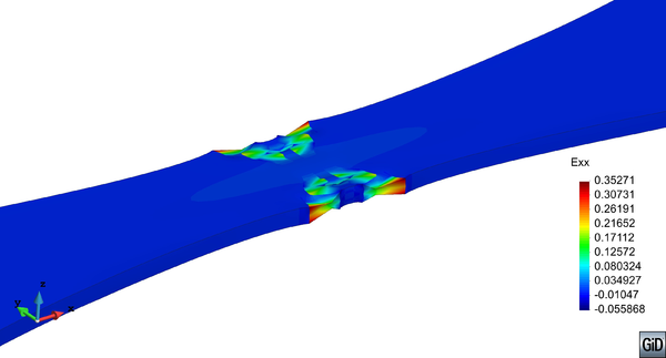
|
| Figure 106: Distribution of the longitudinal strain of the composite in the last step of the analysis on the deformed specimen shape (20x) |
Figure 107 shows the evolution of the curves of interest for the fatigue model at the first integration point where damage initiates in the model. The number of cycles is shown in a logarithmic scale on the horizontal axis. Since damage initiates in the isophtalic matrix these curves refer to the matrix material. In figure 107 the evolution of the equivalent stress in the undamaged space can be seen. This equivalent stress has been calculated with a Von Mises surface and its evolution shows how the load advancing strategy functions at integration point level.
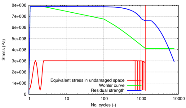
|
| Figure 107: Evolution of the curves of interest for the fatigue model at the first integration point where damage initiates in the model |
First the equivalent stress follows a sinusoidal curve while in the load-tracking stage of the advancing algorithm. When the stress state has stabilized from one cycle to the next in the entire geometry the large increments stage begins, where the applied displacement is maintained constant at its maximum value and the free variable number of cycles increases. In this stage the stress state does not change from one increment to the next, only the material strength threshold and the Wohler Stress change as indicated in figure 107. The strength threshold at that material point is lowered progressively until it reaches the maximum equivalent stress and the damage parameter starts to accumulate. The evolution of the internal damage variable can be seen in figure 108 for the same material point as above. It can be seen that only damage in the matrix accumulates since only the matrix threshold has been surpassed.
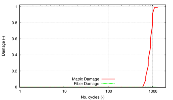
|
| Figure 108: Evolution of the damage internal variables at the first integration point where damage initiates in the model |
The nonlinear stress-strain material behaviour in the isophtalic matrix can be seen in figure 109. When the strength threshold is crossed for the first time a drop in stress is visible. When unloading after this point a corresponding change in stiffness has happened and progressively the matrix load bearing capacity is degraded until failure at that material point. Each jump in stresses is the consequence of another large increment of number of cycles being applied. It can be seen that although the applied maximum displacement of the specimen is constant, a slight reduction of the maximum strain is visible as the stress history of this material point is pushed further in the nonlinear domain. This is a consequence of the structural macro behaviour of the specimen.
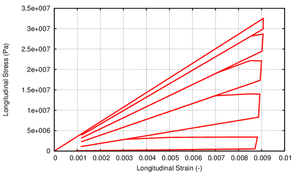
|
| Figure 109: Evolution of the matrix stress-strain at the first integration point where damage initiates in the model |
Following, in figure 110 and figure 111 the fatigue curves of interest are shown in one of the integration points situated in the center of the sample, at the exact position where the strain gauges are located (see figure 97). When assessing the evolution of the equivalent stress in the material, it can be seen that it is virtually unchanged, demonstrating an elastic behaviour, up until the very last analysis steps when there is a sudden increase. This corresponds to the moment in load history when damage has propagated enough into the central width that the remaining material area is unable to bear the applied displacement and sudden structural failure occurs.
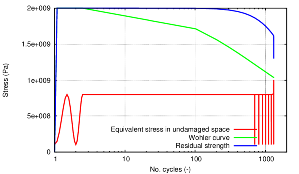
|
| Figure 110: Evolution of the curves of interest for the fatigue model in the fiber of one of the integration points situated at the location of the strain gauge in the experiment |
From figure 110 and figure 111 it can be seen that the behaviour in this model area is the same in both matrix and fiber. The equivalent stress evolution present in the two figures is in accordance to the experimental recordings, indicating a brittle failure mode.
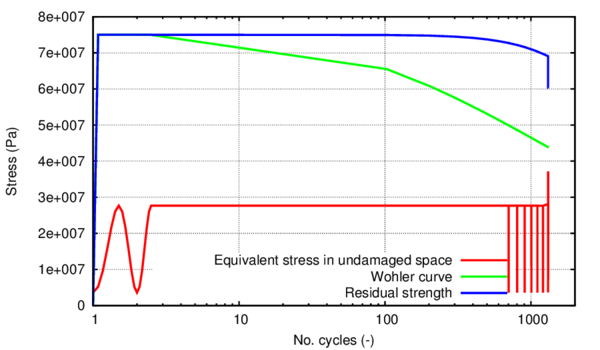
|
| Figure 111: Evolution of the curves of interest for the fatigue model in the matrix of one of the integration points situated at the location of the strain gauge in the experiment |
6.3.4.2 fatigue life curves6.3.4.2
S
−
N
{\displaystyle S-N}
fatigue life curves
The comparison between the numerical and experimental curves is shown in figure 112. These curves are in semi-logarithmic representation. The last point in the chart, corresponding to a ratio of 0.22 between the maximum induced stress at the strain gauge location and the experimentally recorded UTS, represents a cyclic test where the specimen has not failed even after applying 10 cycles of loading both in the numerical simulation and in the experimental test.
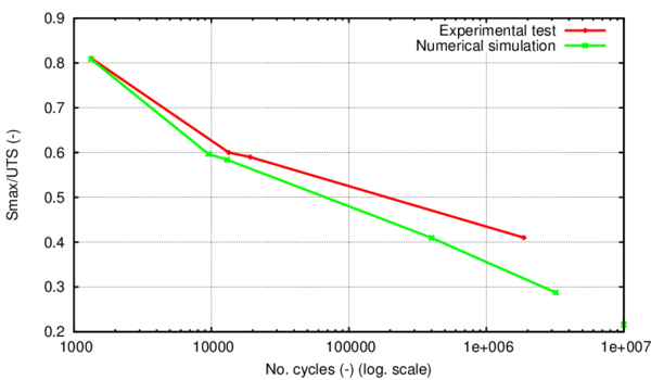
|
| Figure 112: Comparison between the numerical and experimental S-N curves |
The test used in the calibration of the fatigue material parameters and the fracture energy was the first one, where the two curves coincide. The corresponding ratio between the maximum induced stress at the strain gauge location and the experimentally recorded UTS was 0.82. The remaining simulations have been ran with the matrix and fiber material obtained from the calibration process. It can be seen that the life prediction capabilities of the model progressively worsen as the stress ratio lowers.
This tendency can either be a consequence of the test chosen for the calibration; a consequence of the assumptions the model takes into account at splitting the experimental recording into matrix and fiber values, or of the assumption that the fiber and matrix both exhibit nonlinear effects due to fatigue.
In table 23 a summary of all the results, both numerical and experimental, is presented.
| Specimen | Max./ultim. load (%) | Amplitude ratio R | Cycles to failure N (experimental) | Cycles to failure N
(numerical) |
Remarks |
| TP5-1 | 82 | 0.13 | 1346 | 1311 | |
| TP5-2 | 60 | 0.13 | 13407 | 9522 | |
| TP5-3 | 59 | 0.13 | 19159 | 13024 | |
| TP5-4 | 41 | 0.13 | 1875940 | 400020 | |
| 29 | 0.13 | 3200036 | Additional numerical test | ||
| TP5-5 | 22 | 0.15 | 5000000 | 5000000 | not failed |
7 Conclusions
7.1 Final remarks
The aim of this chapter is to summarize all the work done for this monograph highlighting its innovative points and main contributions. This work opens new perspectives to feasible and attractive future developments. The possible lines for future improvements and subsequent developments are also given in this chapter.
The present work aims at advancing an innovative computational methodology that simulates steel and composite fracture under cyclic loading following a phenomenological approach, with calibration from both small scale and large scale testing. This work addresses fatigue processes ranging from high cycle to ultra-low-cycle fatigue.
The general objective of this work was, therefore, the development of a constitutive formulation able to model the entire range of fatigue constitutive behaviour, be it in HCF, ULCF or LCF.
Taking this into consideration, in chapter 3 a new formulation especially developed to simulate the mechanical response of steel, and its failure due to ULCF, has been presented. The formulation is based on the Barcelona plastic model initially proposed by Lubliner et al. [82], which has been improved adding a non-linear kinematic hardening law coupled with two variations of a new isotropic hardening law. In the first case the isotropic hardening law is divided in two regions. In the first one the material exhibits a hardening behaviour and this region is defined by several points that have to be obtained from experimental tests. In the second region, the steel shows a softening behaviour, which is defined with an exponential law. In the second case the curve is divided into three regions: initial hardening obtained by curve fitting to experimental points; a second region, also in hardening, defined by a linear curve with a user imposed slope; and a third region consisting of exponential softening. The evolution of the material in both these two cases is driven by the fracture energy that can be dissipated by the material.
This approach allows predicting material failure by the constitutive model on its own, without the need of additional parameters or additional laws especially chosen for the failure criteria that is to be simulated. Therefore, with the proposed formulation it is possible to simulate accurately the mechanical response of steel under different loading scenarios, such as monotonic, regular cyclic, cyclic followed by a monotonic or a random cyclic load. This last case is equivalent to the load that will be obtained in a seismic case, where ULCF may be one of the main causes of structural failure. Several numerical analyses have been performed in order to show the behaviour of the formulation under the different loading scenarios mentioned.
The capacity of the formulation to simulate accurately the ULCF phenomenon has been proved by reproducing different experimental tests made on X52 steel samples. The experimental campaign consisted in loading several specimens with different strain amplitudes. Tests were also performed to notched specimens in order to increase the plastic strain and reduce the number of cycles that could be applied before failure. One of the experimental tests has been used to calibrate the material parameters of the model; afterwards all other samples have been reproduced numerically. All the numerical results obtained with the proposed constitutive model have provided an excellent agreement with the experimental tests, proving the validity of the proposed formulation to simulate the plastic response of steel and its failure due to ULCF.
After validating the new constitutive law, especially formulated for the monotonic and cyclic behaviour of steel, on small scale specimens, large scale simulations have been conducted to assess its capabilities. Even though the law has been designed for the particular case of cyclic loading, its behaviour was also assessed on a straight pipe loaded monotonically. The results are very promising, with an error of 0.8% in the total axial load at failure for the first case where tension followed by internal pressure was applied. For the second case, internal pressure followed by tension until failure, the error was higher in terms of total axial load, of 9.11%, still below a 10% threshold.
Regarding the ULCF in-plane bending simulations conducted on a 16-inch 90 elbow, the results were in good agreement with the experimental test in terms of force-displacement hysteresis loops and total fatigue life of the specimen, where the error in life prediction was of 5.11% on the safety side for the numerical simulation.
The failure mode obtained by means of the numerical simulation was in agreement to the one found in literature for low internal pressure, but not in agreement with the particular experimental test used for comparison. An analysis of the dependence of the failure mode to the internal pressure applied has been conducted and the limit internal pressure between the two modes has been determined, showing that the formulation is capable of obtaining both failure types.
It should be remarked that the material calibration for both experimental tests reproduced (straight pipe and elbow) has been performed using data from other experimental tests (small samples). This proves the excellent prediction capabilities of the formulation, as it has been able to reproduce accurately the force-displacement response, the maximum load applied and the failure mode in both loading patterns: monotonic and cyclic.
Finally, the main advantage of the model: its ability to predict material failure under a wide variety of non-regular cyclic loads, or under complex loading histories that incorporate monotonic and cyclic episodes, has been emphasized. A seismic-like cyclic displacement has been applied on small scale samples made of X52 steel and the performance of the model has been shown after one and after several cycles of loading.
Chapter 4 has presented a fatigue formulation that takes into account the effects caused by the accumulation of number of cycles of loading thru an alteration in the strength and in the stiffness of the material. First, material strength is reduced until it reaches the induced maximum stress level. From that point on, energy dissipation is done by means of stiffness reduction.
The cyclical load is taken into consideration by means of two parameters: maximum stress generated by the applied load and stress reversion factor. Both parameters have a direct influence on the onset of damage and on the strength reduction. This allows a quantification of the effects induced by different cyclical loads and discrimination between different load-applying orders.
In order to take full advantage of this formulation a stepwise load advancing strategy has been proposed. Its aim is to save computational time and improve convergence in a number of cases, such as load combinations and nonlinear material behaviour.
The procedure divides the load in two different loading processes: load tracking and large increments phases. The jump between the two loading schemes is made automatically, depending on the mechanical response of the structure. The algorithm is user controlled by means of the stabilization tolerance and by the number of cycles considered as large step.
The capabilities of the formulation have been shown in test cases of single cyclical loads and in ones with the load history comprised of two different loads. Validation of the proposed model has been done by reproducing the experimental results obtained by Marines et al. [131].These tests show that, with the strategy proposed, it is possible to perform fatigue simulations taking into account material nonlinearities and load variations straightforward, as the advancing strategy takes care automatically of the procedure required at each step (load-tracking or large increments) in order to obtain the most accurate result with the lowest computational cost.
Chapter 5 describes the formulation for a constitutive model that couples plasticity with damage by a simultaneous integration of the equations of the two processes. The model is energy based and the material performance is determined by the amount of energy dissipated by plasticity and by damage.
This formulation has been applied to cyclical loads and an energy distribution law has been proposed that establishes the energy participation factors for the two processes as a function of the number of cycles the material has been subjected to until having reached softening.
The automated distribution of the energy between the two processes is the main contribution of this work as well as the application of the simultaneous integration scheme for the case of cyclic loading, while considering at the same time both isotropic and kinematic hardening.
The formulation has been implemented to work in the softening regime as damage is a softening process. Comparison to the experimental stress-strain loop has shown the plastic damage model exhibits a behaviour that is closer to the experiment in terms of hysteresis shape and maximum stress reduction, as compared to a formulation using only plasticity equations.
This chapter has also shown that both LCF and ULCF can be simulated with the same thermodynamic framework as the constitutive formulation is able to adapt by itself to the type of fatigue involved.
Chapter 6 has presented the application of the previously shown HCF damage model, coupled with the load-advancing strategy for composite materials. First, material strength has been reduced for each component until it reached the induced maximum stress level in that component. From that point on, energy dissipation has been done by means of stiffness reduction, same as for the model presented in chapter 4.
The constitutive model has been used for both the fiber and the matrix of a composite material and the composite material behaviour has been obtained by means of the serial/parallel rule of mixtures. The fatigue behaviour of the composite has been obtained therefore as a composition of the fatigue of its components. The possibilities of this constitutive strategy have been studied for the case of a pultruded glass fiber reinforced polymer. For this case, a calibration of the material parameters has been made with one of the experimental tests and the resulting material has been used for the rest of the simulations.
The results showed a progressively higher discrepancy between the experimental fatigue life and the numerical one, the lower the maximum stress induced in the specimen is. This tendency is believed to be a consequence of several factors, such as: choosing a skewed test for the calibration; a consequence of the assumptions the model takes into account at splitting the experimental recordings into matrix and fiber values, or of the assumption that the fiber and matrix both exhibit nonlinear effects due to fatigue.
Regarding the failure mode, the experimental results showed diagonal cracks formed in the outer layers containing the combined mats. However, the failure mode in the numerical simulations did not exhibit diagonal cracks. This discrepancy may be due to the fact that the combined mats were not discretized in the numerical model.
Overall, all the objectives defined in the beginning of this document have been achieved. Chapter 3 has adressed the first specific objective of this work; chapter 4 has addressed the second and fourth specific objectives; chapter 5 has addressed the third specific objective of the monograph and the 6th chapter has addressed the last specific objective.
7.2 Future work
This section outlines the possible lines of research opened by this work, as follows:
- The three constitutive formulations shown in this monograph share a common thermodynamic and mechanical framework which offers the possibility of a unified fatigue constitutive formulation that adjusts by itself to the type of problem to be solved (ULCF, HCF or LCF). The preliminary theoretical framework has been addressed by the author in [142] and its implementation is currently work in progress. Chapter 5 has already shown that the consitutive formulation can adapt by itself to LCF and ULCF. The HCF formulation should also be coupled under the same constitutive framework since in real-life simulations it is seldom known beforehand under what type of fatigue failure occurs.
- Mirroring the load-advancing algorithm proposed, a new advancing strategy opens up for ULCF problems where high levels of plastic strain are recorded from the first cycles. Specifically, in the load-tracking stage apart from the characteristics of the stress from one cycle to the next, the energy dissipated is monitored. When the dissipation per cycle reaches a stationary state throughout the continuum a jump can be made where the load is maintained at the maximum level and the dissipation at each Gauss point is incremented with the number of cycles applied as step multiplied by the stabilized dissipation per cycle. The internal variables of the model will then adjust to the new energy state and this procedure can be applied until exhausting all the energy available for hardening, for instance.
- For the case of composite materials only a preliminary study has been made so far. The application of the constitutive formulation to other types of composites (e.g. laminated composites) should be investigated. Following, a generalized application scheme can be derived with a posterior optimization of the constitutive formulation for different types of constituent materials.
- A study on the application of the constitutive models developed in this work is to be made taking into consideration other fields such as aero-generators, structures subjected to vibrations or structures subjected to seismic actions.
- The behaviour of the LCF plastic damage model should be extensively studied for the different cases of cyclic loads, not just for those that induce fatigue lives closer to the ULCF regime but also for the opposite, closer to the HCF regime.
7.3 Innovative contributions
The innovative points of this work can be summarized by the following list:
- Development of a new Barcelona plastic damage model by adding a kinematic and an isotropic constitutive law.
- Characterization of ULCF failure by using the new Barcelona plastic damage model.
- Automatic load-advancing strategy for the resolution of HCF problems.
- Application of the coupled integration scheme to the cyclic problem.
- A fracture energy distribution law for fatigue problems that automatically distributes the energy between damage and plasticity.
- The application of the HCF damage model to composites.
7.4 Publications derived from this work and participation in projects
From the work carried out in the context of this monograph the following publications have resulted:
Peer-reviewed journal publications:
1. Martinez, X., Oller, S., Barbu, L., Barbat, A. and De Jesus, A.M.P. Analysis of ultra-low cycle fatigue problems with the Barcelona plastic damage model and a new isotropic hardening law, International Journal of Fatigue (2015); 73:132-42.
2. Barbu, L.G., Oller, S., Martinez, X. and Barbat, A. High cycle fatigue simulation: A new stepwise load-advancing strategy, Engineering Structures (2015) 97: 118-129, http://dx.doi.org/10.1016/j.engstruct.2015.04.012.
3. Barbu, L.G., Martinez, X., Oller, S. and Barbat, A.H. Validation on large scale tests of a new hardening-softening law for the Barcelona plastic damage model, International Journal of Fatigue (2015); 81:213-226.
4. Barbu, L.G., Oller, S., Martinez, X. and Barbat, A.H. High-cycle fatigue constitutive model for the analysis of fiber reinforced composites, Composite Structures, under review.
5. Barbu, L.G., Oller, S., Martinez, X. and Barbat, A.H. Coupled plastic damage model for the analysis of pipelines under low and ultra-low cycle fatigue, Engineering Fracture Mechanics, under review.
Conference papers:
1. Martinez, X., Oller, S., Barbu, L.G. and Barbat, A.H. Analysis of ultra low cycle fatigue problems with the Barcelona plastic damage model, Proceedings of the 12th International Conference on Computational Plasticity - Fundamentals and Applications, COMPLAS 2013; 352-63.
2. Barbu, L.G., Oller, S., Martínez, X. and Barbat, A.H. Stepwise advancing strategy for the simulation of fatigue problems. Proceedings of the 12th International Conference on Computational Plasticity - Fundamentals and Applications, COMPLAS 2013: 1153-64.
3. Barbu, L.G., Oller, S., Martínez, X. and Barbat, A.H Coupled plastic damage model for low and ultra-low cycle seismic fatigue. 11th. World Congress on Computational Mechanics 2014; 2955-66, ISBN 978-84-942844-7-2.
4. Barbu, L.G., Martinez, X., Oller, S. and Barbat, A.H. Large scale validation of a new isotropic hardening law for the Barcelona plastic damage model under Ultra Low Cycle Fatigue conditions, Proceedings of the 13th International Conference on Computational Plasticity - Fundamentals and Applications, COMPLAS 2015; 248-259.
5. Barbu, L.G., Oller, S., Martínez, X. and Barbat, A.H. Model-wise algorithm for the resolution of fatigue problems, Proceedings of the 13th International Conference on Computational Plasticity - Fundamentals and Applications, COMPLAS 2015; 260-271.
Projects:
Ultra low cycle fatigue of steel under cyclic high-strain loading conditions Funded by the Research Fund for Coal and Steel thru grant no. RFSR-CT-2011-00029 Starting date: 01/07/2011 End date: 30/06/2014
Conference attendance with presentation:
1. Barbu, L.G., Oller, S., Martinez, X. and Barbat, A.H. Plastic damage model for fatigue in composites. ICCS18 (18th International Conference on Composite Structures), Lisbon, Portugal, 15-18 June 2015.
References
[1] ASTM Standard E1823-13. Standard terminology relating to fatigue and fracture testing. ASTM International, West Conshohocken, PA, 2013
[2] Oller, S. and Salomón, O. and Oñate, E.. A continuum mechanics model for mechanical fatigue analysis, Volume 32. Comp. Mater. Sci. 2 175 - 195, 2005
[3] A.M. Kanvinde and G.G. Deierlein. Cyclic Void Growth Model to Assess Ductile Fracture Initiation in Structural Steels due to Ultra Low Cycle Fatigue, Volume 133. J. Eng. Mech. 6 701 - 712, 2007
[4] Kanvinde, A.M. and Deierlein, G.G.. Micromechanical simulation of earthquakeinduced fracture in steel structures, 2004
[5] Xue, L.. A unified expression for low cycle fatigue and extremely low cycle fatigue and its implication for monotonic loading, Volume 30. Int. J. Fat. 1691- 1698, 2008
[6] F.C. Campbell. Elements of Metallurgy and Engineering Alloys. ASM International, Ohio, USA, 2008
[7] Zhou, J. and Horsley, D. and Rothwell, B.. Application of strain-based design for pipelines in permafrost areas, 2006
[8] EWI. Strain-Based Design of Pipelines. U.S. Department of Interior, 2003
[9] Liu, Bing and Liu, X.J. and Zhang, Hong. Strain-based design criteria of pipelines, Volume 22. Journal of Loss Prevention in the Process Industries 6 884-888, 2009
[10] Yao, J. T. P. and Munse, W. H.. Low-cycle fatigue of metals–literature review. Serial no. SSC-137, first progress report of project SR-149 to the ship structure committee on low-cycle fatigue of metals - literature review., 1961
[11] Solomon, H.D. and Halford, G.R. and Kaisand, L.R. and Leis, B.N.. Low cycle fatigue: directions for the future, 1988
[12] Kuroda, M.. Extremely low cycle fatigue life prediction based on a new cumulative fatigue damage model, Volume 24. Int J Fatigue 6 699 - 703, 2002
[13] Tateishi, K. and Hanji, T. and Minami, K.. A prediction model for extremely low cycle fatigue strength of structural steel, Volume 29. Int J Fatigue 5 887 - 896, 2007
[14] Ohata, M. and Toyoda, M.. Damage concept for evaluating ductile cracking of steel structure subjected to large-scale cyclic straining, Volume 5. Sci. Technol. Adv. Mater. 1-2 241 - 249, 2004
[15] J.-B. Leblond and G. Perrin and J. Devaux. An improved Gurson-type model for hardenable ductile metals, Volume 14. Eur.J. Mech. A-Solids 499 - 527, 1995
[16] Pirondi, A. and Bonora, N.. Modeling ductile damage under fully reversed cycling, Volume 26. Comput. Mater. Sci. 129 - 141, 2003
[17] Kanvinde, A.M. and Deierlein, G.G.. Void growth model and stress modified critical strain model to predict ductile fracture in structural steels, Volume 132. J Struct Eng 2 1907 - 1918, 2006
[18] Rice, J. R. and Tracey, D.M.. On the ductile enlargement of voids in triaxial stress fields, Volume 35. J. Mech. Phys. Solids 201 - 217, 1969
[19] J. W. Hancock and A.C. Mackenzie. On the mechanics of ductile failure in high-strength steel subjected to multiaxial stress states, Volume 24. J. Mech. Phys. Solids 3 147 - 169, 1976
[20] J. Lemaitre. A Continuous Damage Mechanics Model for Ductile Fracture, Volume 107. J. Eng. Mater. Technol. 83 - 89, 1985
[21] J. L. Chaboche. Anisotropic damage in the framework of the continuum damage mechanics, Volume 79. Nucl. Eng. Des. 309 - 319, 1984
[22] Jiang, Y. and Ott, W. and Baum, C. and Vormwald, M. and Nowack, H.. Fatigue life predictions by integrating EVICD fatigue damage model and an advanced cyclic plasticity theory, Volume 25. Int J Plast 5 780 - 801, 2009
[23] Nowack, H. and Hanschmann, D. and Ott, W. and Trautmann, K.H. and Maldfeld, E.. Crack initiation life behaviour under biaxial loading conditions: experimental behaviour and prediction, Volume 12. Multiaxial Fatigue Deform Test Techn 159- 183, 1996
[24] Ott, W. and Baumgart, O. and Trautmann, K.H. and Nowack, H.. A new crack initiation life prediction method for arbitrary multiaxial loading considering mean stress effect 1007 - 1012, 1996
[25] Saanouni, K. and Abdul-Latif, A.. Micromechanical modeling of low cycle fatigue under complex loading – Part I. Theoretical formulation, Volume 12. Int J Plast 9 1111 - 1121, 1996
[26] Abdul-Latif, A. and Saanouni, K.. Micromechanical modeling of low cycle fatigue under complex loadings – Part II, Application, Volume 12. Int J Plast 9 1123 - 1149, 1996
[27] Naderi, M. and Hoseini, S.H. and Khonsari, M.M.. Probabilistic simulation of fatigue damage and life scatter of metallic components, Volume 43. Int J Plast 101 - 115, 2013
[28] J. Lemaitre and J.-L. Chaboche.. Mechanics of Solid Materials. Cambridge University Press. New York, USA, 1990
[29] Warhadpande, A. and Jalalahmadi, B. and Slack, T. and Sadeghi, F.. A new finite element fatigue modeling approach for life scatter in tensile steel specimens, Volume 32. Int J Fatigue 4 685 - 697, 2010
[30] Schijve, J.. Fatigue of Structures and Materials. Berlin: Springer-Verlag, 2 Edition, 2009
[31] Fatemi, A. and Yang, L.. Cumulative fatigue damage and life prediction theories: a survey of the state of the art for homogeneous materials, Volume 20. Int J Fat 9 - 34, 1998
[32] Kachanov, L. M.. Time to the rupture process under creep conditions, Volume 8. Izv. Akad. Nauk. SSR Otd. Tech. Nauk. 26 - 31, 1958
[33] Kachanov, L.M.. Introduction to continuum damage mechanics. Martinus, Nijhoff Publisher, Boston- Dordrecht., 1986
[34] Chaboche, J.L.. Fracture mechanics and damage mechanics: complementarity of approaches 309 - 324, 1987
[35] Chaboche, J.L.. A differential law for nonlinear cumulative fatigue damage, Volume 39. In Materials and Building Research, Annales de l’ITBTP 117 - 124, 1974
[36] Lemaitre, J. and Chaboche J. L.. Aspect phenomenologique de la rupture par endommagement, Volume 2. J Mech App 3 317 - 365, 1978
[37] Wang, J.. A continuum damage mechanics model for low-cycle fatigue failure of metals, Volume 41. Engng Fract Mech 3 437 - 441, 1992
[38] Wang, T. and Lou, Z.. A continuum damage model for weld heat affected zone under low-cycle fatigue loading, Volume 37. Engng Fract Mech 4 825 - 829, 1990
[39] Li, C. and Qian, Z. and Li, G.. The fatigue damage criterion and evolution equation containing material microparameters, Volume 34. Engng Fract Mech 2 435 - 443, 1989
[40] Holman, R. K. and Liaw, P. K.. Methodologies for predicting fatigue life, Volume 49. JOM: the journal of the Minerals, Metals & Materials Society 7 46 - 52, 1997
[41] Palmgren, A.. Die Lebensdauer von Kugellagern (The service life of ball bearings), Volume 68. Zeitschrift des Vereines Deutscher lngenieure 14 339 - 341, 1924
[42] Miner, M.. Cumulative fatigue damage, Volume 12. J. App. Mech. 3 159 - 164, 1945
[43] Vasudevan,A.K and Sadananda, K. and Glinka, G.. Critical parameters for fatigue damage, Volume 23. Int J Fat 1 39 - 53, 2001
[44] Halford, G.R.. Cumulative fatigue damage modeling—crack nucleation and early growth, Volume 19. Int J Fat 1 5253 - 5260, 1997
[45] Hoeppner, D. W. and Krupp, W.. Prediction of component life by application of fatigue crack growth knowledge, Volume 6. Engng Fract Mech 47 - 70, 1974
[46] A. L. Gurson. Continuum theory of ductile rupture by void nucleation and growth: part i - yield criteria and flow rules for porous ductile media, Volume 99. J. Eng. Mater. Technol. 2 - 15, 1977
[47] Needleman, A. and Tvergaard, V.. An analysis of ductile rupture modes at the crack tip, Volume 35. J. Mech. Phys. Solids 151 - 183, 1987
[48] F. L. Addessio and J. N. Johnson. Rate-dependent ductile failure model, Volume 74. J. Appl. Phys. 3 1640 - 1648, 1993
[49] N. Bonora. Ductile damage parameters identification and measurement, Volume 34. J. Strain Anal. 6 463 - 478, 1999
[50] Y. Bao and T. Wierzbicki. On Fracture Locus in the equivalent Strain and Stress Triaxiality Space, Volume 46. Int. J. Mech. Sci. 81 - 89, 2004
[51] D.P. Clausing. Effect of Plastic Strain State on Ductility and Toughness, Volume 6. Int. J. Fract. Mech. 71 - 85, 1970
[52] McClintock, F.A.. Plasticity Aspects on Fracture. Fracture, H. Liebowitz, Ed., Vol. 3, Academic Press, New York, pp. 47-225., 1971
[53] Wierzbicki, T. and Bao, Y. and Lee, Y-W. and Bai, Y.. Calibration and Evaluation of Seven Fracture Models, Volume 47. Int. J. Mech. Sci. 719 - 743, 2005
[54] I. Barsoum and J. Faleskog. Rupture Mechanisms in Combined Tension and Shear - Experiment, Volume 44. Int. J. Solids Struct. 1768 - 1786, 2007
[55] T. Coppola and L. Cortese and P. Folgarait. The effect of stress invariants on ductile fracture limit in steels, Volume 76. Eng. Fract. Mech. 1288 - 1302, 2009
[56] Commission on Engineering and Technical Systems. Assessment of Research Needs for Wind Turbine Rotor Materials Technology.. Washington, D.C.: National Academy Press., 1991
[57] R.J. Huston. Fatigue life prediction in composites, Volume 59. Journal of Pressure Vessel Technology 131 - 140, 1994
[58] A. S. Chen and D.P. Almond and B. Harris. Real time monitoring of fatigue-induced damage growth in composite materials by Acoustography, Volume 61. Composite Sci. & Tech. 2437 - 2444, 2001
[59] Schulz, A. and Sayer,F. and van Wingerde, A.. Experimental investigation of the influence of ply-drop geometry on the fatigue behavior of tapered composites, 2011
[60] Firehole Composites. Fatigue life prediction in composite materials. Available from: http://www.firehole.com/documents/ WP_Fatigue-Life-Prediction-in-Composite-Materials.pdf, 2010
[61] Z. Hashin and A. Rotem. A fatigue failure criterion for fiber reinforced materials, Volume 7. Journal of Composite Materials 448 - 464, 1973
[62] Halpin, J.C. and Johnson, T.A. and Waddups, M.E.. Kinetic fracture models and structural reliability, Volume 8. Int J Fract Mech 465 - 468, 1972
[63] K.L. Reifsnider. The critical element model: A modeling philosophy, Volume 25. Eng Fract Mech 739 - 749, 1986
[64] K.L. Reifsnider and W.W. Stinchcomb. A critical element model of the residual strength and life of fatigue-loaded composite coupons, Volume 907. Composite Materials: Fatigue and Fracture, ASTM STP 298 - 313, 1986
[65] H.G. Halvarson and W.A. Curtin and K.L. Reifsnider. Fatigue life of individual composite specimens based on intrinsic fatigue behavior, Volume 19. Int J Fatigue 5 369 - 377, 1996
[66] K.L. Reifsnider and S. Case and J. Duthoit. The mechanics of composite strength evolution, Volume 60. Compos Sci Tech 2539 - 2546, 2000
[67] T.K. O’Brien and K.L. Reifsnider. Fatigue damage evaluation through stiffness measurements in boron epoxy laminates, Volume 15. J Compos Mat 55 - 70, 1981
[68] D.Y. Song and N. Otani. Fatigue life prediction of cross-ply composite laminates, Volume A238. Mat Sci Eng 329 - 335, 1977
[69] A. Charewicz and I.M. Daniel. Damage mechanisms and accumulation in graphiteepoxy laminates, Volume 907. Composite Materials: Fatigue and Fracture, ASTM STP 274 - 297, 1986
[70] E.K. Gamstedt and B.A. Sjögren. An experimental investigation of the sequence effect in block amplitude loading of crossply composite laminates, Volume 24. Int J Fatigue 437 - 446, 2002
[71] T.P. Philippidis and V.A. Passipoularidis. Residual strength after fatigue in composites: Theory vs. experiment, Volume 29. Int J Fatigue 12 2104 - 2116, 2007
[72] L.J. Broutman and S. Sahu. A new theory to predict cumulative fatigue damage in fiberglass reinforced plastics, Volume 497. Composite materials: testing and design (2nd Conference), ASTM STP 170 - 188, 1972
[73] T. Adam and R.F. Dickson and C.J. Jones and H. Reiter and B. Harris. A power law fatigue damage model for fiber reinforced plastic laminates, Volume 200. Proc Instn Mech Engrs C3 155- 166, 1986
[74] X. Martinez and S. Oller and E. Barbero. Study of delamination in composites by using the serial/parallel mixing theory and a damage formlation, 2007
[75] Mayugo, J.A.. Estudio constitutivo de materiales compuestos laminados sometidos a cargas ciclicas. Universitat Politecnica de Catalunya, 2003
[76] Coffin, L. F.. Low cycle fatigue-a review, Volume 1. Appl. Mater. Res. 3 129 - 141, 1962
[77] Anderson, T. L.. Fracture mechanics. CRC, Boca Raton, Fla., 1995
[78] Kuwamura, H. and Yamamoto, K.. Ductile crack as a trigger of brittle fracture in steel, Volume 123. J. Struct. Eng. 6 729 - 735, 1997
[79] Manson, S.S.. Behavior of materials under conditions of thermal stress, 1954
[80] Paris, P. and Erdogan, F.. A Critical Analysis of Crack Propagation Laws, Volume 85. ASME, J. Basic Engrg. 528 - 534, 1963
[81] Tatsuo, E. and Koichi, M. and Kiyohumi, T. and Kakuichi, K. and Masanori M.. Damage evaluation of metals for random of varying loading -Three aspects of rain flow method, 1974
[82] J. Lubliner and J. Oliver and S. Oller and Oñate, E.. A plastic damage model for concrete, Volume 25. International Journal of Solids and Structures 3 299 - 326, 1989
[83] S. Oller and J. Oliver and J. Lubliner and Oñate, E.. Un Modelo Constitutivo de Daño Plástico Para Materiales Friccionales: Parte I, Variables Fundamentales, Funciones de Fluencia y Potencial, Volume 4. Rev Int Métodos Numér para el Cálculo y diseño en Ing 4 397 - 431, 1988
[84] S. Oller and J. Oliver and J. Lubliner and Oñate, E.. Un Modelo Constitutivo de Daño Plástico Para Materiales Friccionales: Parte II, Generalización para Procesos con Degradación de Rigidez, Volume 4. Rev Int Métodos Numér para el Cálculo y diseño en Ing 4 433 - 461, 1988
[85] Lee, J. and Fenves, G.. Plastic-Damage Model for Cyclic Loading of Concrete Structures, Volume 124. Journal of Engineering Mechanics 8 892 - 900, 1998
[86] Martinez, X. and Oller, S. and Barbu, L.G. and Barbat, A.. Analysis of ultra-low cycle fatigue problems with the Barcelona plastic damage model 352 - 363, 2013
[87] Martinez, X. and Oller, S. and Barbu, L.G. and Barbat, A. and De Jesus, A.M.P.. Analysis of ultra-low cycle fatigue problems with the Barcelona plastic damage model and a new isotropic hardening law, Volume 73. Int. J. Fatigue 132 - 142, 2015
[88] Barbu, L.G. and Martinez, X. and Oller, S. and Barbat, A.H.. Validation on large scale tests of a new hardening-softening law for the Barcelona plastic damage model, Volume 81. Int. J. Fat. 213 - 226, 2015
[89] B. Luccioni and S. Oller and R. Danesi. Coupled plastic damaged model, Volume 129. Computer Methods in Applied Mechanics and Engineering 1-2 81 - 89, 1996
[90] Sergio Oller. Fractura mecánica. Un enfoque global.. Centro Internacional de Métodos Numéricos en Ingeniería - CIMNE, 2001
[91] Lubliner, J.. On thermodyamics foundations of non-linear solid mechanics, Volume 7. International Journal non-linear Mechanics 237- 254, 1972
[92] Lubliner, J.. Plasticity Theory. Macmillan Publishing. New York, USA, 1990
[93] A. Green and P. Naghdi. A general theory of an elastic-plastic continuum, Volume 18. Archive for rational mechanics and analysis 4 251 - 281, 1964
[94] L. E. Malvern. Introduction to the mechanics of a continuous medium, 1969
[95] Maugin, G.. The Thermomechanics of Plasticity and Fracture. Cambridge University Press. New York, USA, 1992
[96] B.K. Chun and J.T. Jinna and J.K. Lee. Modeling the Bauschinger effect for sheet metals. Part I: theory, Volume 18. International Journal of Plasticity 571 - 595, 2002
[97] M.E. Kassner and P. Geantil and L.E. Levine and B.C. Larson. Backstress, the Bauschinger Effect and Cyclic Deformation, Volume 604-605. Materials Science Forum 39 - 51, 2009
[98] Oller, S.. Nonlinear dynamics of structures. Springer, 2014
[99] X. Martinez and S. Oller and F. Rastellini and A.H. Barbat. A numerical procedure simulating RC structures reinforced with FRP using the serial/parallel mixing theory, Volume 86. Computers and Structures, 2008
[100] Martinez, X. and Oller, S. and Barbero, E.. Mechanical response of composites. Chapter: Study of delamination in composites by using the serial/parallel mixing theory and a damage formulation. ECCOMAS series Edition, Springer, 2008
[101] Pereira, J.C.R. and de Jesus, A.M.P. and Xavier, J. and Fernandes, A.A. and Martins, B.. Comparison of the monotonic, low-cycle and ultra-low-cycle fatigue behaviors of the X52, X60 and X65 piping steel grades, 2014
[102] PLCd research group. PLCd: Non-linear thermo-mechanic finite element code for research-oriented applications. Free access code developed at CIMNE. Available from: http://www.cimne.com/PLCd, 1991-to present
[103] Barbu, L.G. and Oller, S. and Martinez, X. and Barbat, A.H.. Stepwise advancing strategy for the simulation of fatigue problems 1153 – 1164, 2013
[104] Barbu, L.G. and Oller, S. and Martinez, X. and Barbat, A.H.. High cycle fatigue simulation: A new stepwise load-advancing strategy, Volume 97. Engineering Structures 118 - 129, 2015
[105] Schaffrath, S. and Novokshanov, D. and Eichler, B. and Münstermann, S.. Characterization and simulation of X60 elbow pipes in case of ULCF loading, 2014
[106] ECCS Technical Committee 13. Recommended testing procedures for assessing the behaviour of structural steel elements under cyclic loads, 1986
[107] Sobel, L.H. and Newman, S.Z.. Comparison of Experimental and Simplified Analytical Results for the In-Plane Plastic Bending and Buckling of an Elbow, Volume 102. ASME J. Pressure Vessel Technol. 400 - 409, 1980
[108] Sobel, L.H. and Newman, S.Z.. Simplified, Detailed and Isochronous Analysis and Test Results for the In-Plane Elastic-Plastic and Creep Behaviour of an Elbow, Volume 108. ASME J. Pressure Vessel Technol. 297 - 304, 1986
[109] Dhalla, A.K.. Collapse Characteristics of a Thin-Walled Elbow, Volume 109. ASME J. Pressure Vessel Technol. 394 - 401, 1987
[110] Greenstreet, W.L.. Experimental Study of Plastic Responses of Pipe Elbows, 1978
[111] Tan, Y. and Matzen, V. C. and Yu, L. X.. Correlation of Test and FEA Results for the Nonlinear Behavior of Straight Pipes and Elbows, Volume 124. ASME J. Pressure Vessel Technol. 4 465 - 475, 2002
[112] Shalaby, M. A. and Younan, M. Y. A.. Limit Loads for Pipe Elbows With Internal Pressure Under In-Plane Closing Bending Moments, Volume 120. ASME J. Pressure Vessel Technol. 1 35 - 42, 1998
[113] Suzuki, N. and Nasu, M.. Non-Linear Analysis of Welded Elbows Subjected to In-Plane bending, Volume 32. Computers and Structures 3/4 871 - 881, 1989
[114] Yahiaoui, K. and Moffat, D.G. and Moreton, D.N.. Response and cyclic strain accumulation of pressurized piping elbows under dynamic in-plane bending, Volume 31. J. Strain Analysis for Engrg Design 2 135 - 151, 1996
[115] Slagis, G.C.. Experimental Data on Seismic Response of Piping Components, Volume 120. ASME J. Pressure Vessel Technol. 449 - 455, 1998
[116] Fujiwaka, T. and Rndou, R. and Furukawa, S. and Ono, S and Oketani, K.. Study on strength of piping components under elastic-plastic behavior due to seismic loading, 1999
[117] Karamanos, S. A. and Giakoumatos, E. and Gresnigt, A. M.. Nonlinear Response and Failure of Steel Elbows Under In-Plane Bending and Pressure, Volume 125. ASME J. Pressure Vessel Technol. 4 393 - 402, 2003
[118] Karamanos, S. A. and Tsouvalas, D. and Gresnigt, A. M.. Ultimate Bending Capacity and Buckling of Pressurized 90 Deg Steel Elbows, Volume 128. ASME J. Pressure Vessel Technol. 3 348 - 356, 2006
[119] Pappa, P. and Tsouvalas, D. and Karamanos, S. A. and Houliara, S.. Ultimate Capacity of Pipe Bends Under Bending and Pressure, 2008
[120] Varelis, G. E. and Karamanos, S. A. and Gresnigt, A. M.. Pipel Elbows Under Strong Cyclic Loading, Volume 135. ASME J. Pressure Vessel Technol. 1 011207, 2013
[121] Varelis, G. E. and Ferino, J. and Karamanos, S. A. and Lucci, A. and Demofonti, G.. “Experimental and Numerical Investigation of Pressurized Pipe Elbows Under Strong Cyclic Loading, 2013
[122] Coppola, T. and Iob, F. and Karamanos, S. and Varelis, G. and Schaffrath, S. and Feldman, M. and Thibaux, P.. Large scale monotonic and cyclic tests of pipeline components, 2013
[123] Bathias, C.. There is no infinite fatigue life in metallic materials, Volume 22. Fat Fract Eng Mat Struct 559 - 565, 1999
[124] Bathias, C. and Ni, J.. Determination of fatigue limit between 105 and 109 cycles using an ultrasonic fatigue device, Volume 2. Advance in Fatigue Lifetime Predictive Techinques, ASTM STP 1211 141 - 152, 1993
[125] Marines, I. and Bin, X. and Bathias, C.. An understanding of very high cycle fatigue of metals, Volume 25. Int J Fat 1101 - 1107, 2003
[126] Simo, J. and Ju, J.. Strain and stress based continuum damage models – I Formulation, Volume 23. Int J Solids Struct 821 - 840, 1987
[127] Oliver, J. and Cervera, M. and Oller, S. and Lubliner, J.. Isotropic damage models and smeared crack analysis of concrete, Volume 2 945 - 958, 1990
[128] Salomón, O. and Oller, S. and Oñate, E.. Fatigue Analysis of Materials and Structures Using a Continuum Damage Model, Volume 5. Int J Forming Processes 493 - 503, 2002
[129] Suero, A. and Oller, S.. Tratamiento del Fenómeno de Fatiga Mediante la Mecánica de Medios Continuos. Centro Internacional de Métodos Numéricos en Ingeniería - CIMNE, Monography No. 45, Barcelona, Spain, 1998
[130] S. Oller and Oñate, E. and J. Miquel and S. Botello. A plastic damage constitutive model for composite materials, Volume 33. International Journal of Solids and Structures 17 2501 - 2518, 1996
[131] Marines, I. and Galván, D. and Bathias, C.. Fatigue life assessment of high-strength, low alloy steel at high frequency, Volume 33. Arabian J Sci Eng 1B 237 - 247, 2008
[132] K. Kimishima and Y. Maruyama and F. Yamazaki. Damage Ratio of Water Pipes during the 2007 Niigata-Ken Chuetsu-Oki, Japan, Earthquake, Volume 14. Procedia Engineering 212 - 219, 2011
[133] Armero, F. and Oller, S.. A general framework for continuum damage models. I. Infinitesimal plastic damage models in stress space, Volume 37. International Journal of Solids and Structures 48-50 7409 - 7436, 2000
[134] Armero, F. and Oller, S.. A general framework for continuum damage models. II. Integration algorithms, with appliactions to the numerical simulation of porous metals, Volume 37. International Journal of Solids and Structures 48-50 7437 - 7464, 2000
[135] Barbu, L.G. and Oller, S. and Martinez, X. and Barbat, A.H.. Coupled plastic damage model for low and ultra-low cycle seismic fatigue 2955-2966, 2014
[136] Oller, S.. Modelización Numérica de Materiales Friccionales. Centro Internacional de Métodos Numéricos en Ingeniería - CIMNE, Monography No. 3, Barcelona, Spain, 1991
[137] Zienkiewicz, O. C. and Taylor, R.. The Finite Element Method, Volume 1,2. Butterworth-Heinemann, 5 Edition, 2000
[138] F. Rastellini and S. Oller and O. Salomón and Oñate, E.. Composite materials non-linear modelling for long fibre-reinforced laminates continuum basis, computational aspect and validations, Volume 86. Computers and Structures 879 - 896, 2008
[139] O. Salómon and F. Rastellini and S. Oller and E. Oñate. Fatigue prediction for composite materials and structures, 2005
[140] T. Keller and T. Tirelli and A. Zhou. Tensile fatigue performance of pultruded glass fiber reinforced polymer profiles, Volume 68. Compos Struct 2 235 - 245, 2005
[141] Keller, T. and Tirelli, T.. Fatigue behavior of adhesively connected pultruded GFRP laminates, Volume 65. Compos Struct 1 55 - 64, 2004
[142] Barbu, L.G. and Oller, S. and Martinez, X. and Barbat, A. H.. Model-wise algorithm for the resolution of fatigue problems 260 - 271, 2015
Document information
Published on 15/02/18
Submitted on 15/02/18
Licence: CC BY-NC-SA license
Share this document
claim authorship
Are you one of the authors of this document?

