A simple overview of least squares

1 Introduction

In mathematics, the term least squares refers to an approach for “solving” overdetermined linear or nonlinear systems of equations. A common problem in science is to fit a model to noisy measurements or observations. Instead of solving the equations exactly, which in many problems is not possible, we seek only to minimize the sum of the squares of the residuals.

The algebraic procedure of the method of least squares was first published by Legendre in 1805 [1]. It was justified as a statistical procedure by Gauss in 1809 [2], where he claimed to have discovered the method of least squares in 1795 [3]. Robert Adrian had already published a work in 1808, according to [4]. After Gauss, the method of least squares quickly became the standard procedure for analysis of astronomical and geodetic data. There are several good accounts of the history of the invention of least squares and the dispute between Gauss and Legendre, as shown in [3] and references therein. Gauss gave the method a theoretical basis in two memoirs [5], where he proves the optimality of the least squares estimate without any assumptions that the random variables follow a particular distribution. In an article by Yves [6] there is a survey of the history, development, and applications of least squares, including ordinary, constrained, weighted, and total least squares, where he includes information about fitting curves and surfaces from ancient civilizations, with applications to astronomy and geodesy.

The basic modern numerical methods for solving linear least squares problems were developed in the late 1960s. The ${\textstyle QR}$ decomposition by Householder transformations was developed by Golub and published in 1965 [7]. The implicit ${\textstyle QR}$ algorithm for computing the singular value decomposition (SVD) was developed by Kahan, Golub, and Wilkinson, and the final algorithm was published in 1970 [8]. Both fundamental matrix decompositions have since been developed and generalized to a high level of sophistication. Since then great progress has been made in methods for generalized and modified least squares problems in direct, and iterative methods for large sparse problems. Methods for total least squares problems, which allow errors also in the system matrix, have been systematically developed.

In this work we aim to give a simple overview of least squares for curve fitting. The idea is to illustrate, for a broad audience, the mathematical foundations and practical methods to solve this simple problem. Particularly, we will consider four methods: the normal equations method, the QR approach, the singular value decomposition (SVD), as well as a more recent approach based on neural networks. The last one has not been used as frequently as the classical ones, but it is very interesting because in modern days it has become a very important tool in many fields of modern knowledge, like data science (DS), machine learning (ML) and artificial intelligence (AI).

2 Linear least squares for curve fitting and the normal equations

There are many problems in applications that can be addressed using the least squares approach. A common source of least squares problems is curve fitting. This is the one of the simplest least squares problems, but still it is a very fundamental problem, which contains all important ingredients of commonly ill posed problems and, even worse, they may be ill conditioned and difficult to compute with good precision using finite (inexact) arithmetic in modern computer devices. We start with the linear least squares problem.

Let’s assume that we have ${\textstyle m}$ noisy experimental observations (points)

$(t_{1},{\hat {y}}_{1}),(t_{2},{\hat {y}}_{2}),\ldots ,(t_{m},{\hat {y}}_{m}),$

which relate two real quantities, as shown in figure 2. We want to fit a curve, represented by a real scalar function ${\textstyle y(t)}$, to the given data. A linear model for the unknown curve can be represented as a linear combination of given (known) base functions ${\textstyle \phi _{1}}$, ${\textstyle \phi _{1}}$,...,${\textstyle \phi _{n}}$:

$y(t)=c_{1}\phi _{1}(t)+c_{2}\phi _{2}(t)+\ldots +c_{n}\phi _{n}(t),$

(1)

where ${\textstyle c_{1},c_{2},\ldots c_{n}}$ are unknown coefficients. A first naive approach to compute those coefficients is assuming that ${\textstyle {\hat {y}}_{i}=y(t_{i})}$ for each ${\textstyle i=1,2,\ldots ,m}$. This assumption yields the linear system ${\textstyle {\hat {y}}_{i}=c_{1}\phi _{1}(t_{i})+c_{2}\phi _{2}(_{i})+\ldots +c_{n}\phi _{n}(t_{i})}$, ${\textstyle i=1,2,\ldots ,m}$, which can be represented as ${\textstyle A\,\mathbf {x} =\mathbf {b} }$, where

$A=\left[{\begin{array}{cccc}\phi _{1}(t_{1})&\phi _{2}(t_{1})&\ldots &\phi _{n}(t_{1})\\\phi _{1}(t_{2})&\phi _{2}(t_{2})&\ldots &\phi _{n}(t_{2})\\\vdots &&\ddots &\vdots \\\phi _{1}(t_{m})&\phi _{2}(t_{m})&\ldots &\phi _{n}(t_{m})\end{array}}\right],\qquad \mathbf {x} =\left[{\begin{array}{c}c_{1}\\c_{2}\\\vdots \\c_{n}\end{array}}\right],\qquad \mathbf {b} =\left[{\begin{array}{c}{\hat {y}}_{1}\\{\hat {y}}_{2}\\\vdots \\{\hat {y}}_{m}\end{array}}\right],$

Depending on the problem or application, the base functions ${\textstyle \phi _{j}}$, ${\textstyle 1\leq j\leq n}$, may be polynomials ${\textstyle \phi _{j}(t)=t^{j-1}}$, exponentials ${\textstyle \phi _{j}(t)=e^{\lambda _{j}\,t}}$, log-linear ${\textstyle \phi =K\,e^{\lambda \,t}}$, among many others.

There are some drawbacks and difficulties with the previous approach: vector ${\textstyle \mathbf {b} }$ must belong to the column space of ${\textstyle A}$, denoted by ${\textstyle \operatorname {Col} (A)}$, in order to get solution(s) of the linear system. The rank of ${\textstyle A}$ is ${\textstyle r=\dim \operatorname {Col} (A)}$, and plays a important role. When ${\textstyle m>r}$, most likely ${\textstyle \mathbf {b} \notin \operatorname {Col} (A)}$, and the system has no solution; if ${\textstyle m<r}$, the undetermined linear system has infinite many solutions; finally, when ${\textstyle m=r}$, if the system has a solution, the computed curve produces undesirable oscillations, specially near the far right and left points, a well known phenomenon in approximation theory and numerical analysis, known as the Runge's phenomenon [9], demonstrating that high degree interpolation does not always produce better accuracy. The least squares approach considers the residuals, which are the differences between the observations and the model values:

$r_{i}={\hat {y}}_{i}-\sum _{j=1}^{n}c_{j}\,\phi _{j}(t_{i})\quad {\hbox{or}}\quad \mathbf {r} =\mathbf {b} -A\,\mathbf {x} .$

Ordinary least squares to find the best fitting curve ${\textstyle y(t)}$, consists in finding ${\textstyle \mathbf {x} }$ that minimizes the sum of squared residuals

$\|\mathbf {r} \|^{2}=\sum _{j=1}^{n}r_{i}^{2}=\Vert \mathbf {b} -A\,\mathbf {x} \Vert ^{2}.$

The least squares criterion has important statistical interpretations, since the residual ${\textstyle r_{i}}$ in

${\hat {y}}_{i}=y(t_{i})+r_{i},$

may be considered as a measurement error with a given probabilistic distribution. In fact, least squares produces what is known as the maximum-likelihood estimate of the parameter estimation of the given distribution. Even if the probabilistic assumptions are not satisfied, years of experience have shown that least squares produces useful results.

2.1 The normal equations

The quadratic function ${\textstyle f(\mathbf {x} )=\Vert \mathbf {b} -A\,\mathbf {x} \Vert ^{2}=\mathbf {x} ^{T}A^{T}A\,\mathbf {x} -2\mathbf {x} ^{T}A^{T}\mathbf {b} +\mathbf {b} ^{T}\mathbf {b} }$ has gradient and Hessian given by ${\textstyle \nabla f(x)=2\,A^{T}A\,\mathbf {x} -2\,A^{T}\mathbf {b} }$ and ${\textstyle H_{f}(\mathbf {x} )=2\,A^{T}A}$, respectively. Assuming that the design matrix ${\textstyle A}$ has full rank, then the Hessian is positive definite, thus invertible, because ${\textstyle A^{T}A}$ is an ${\textstyle n\times n}$ symmetric matrix, and positive definite since ${\textstyle \mathbf {x} ^{T}A^{T}A\,\mathbf {x} =||A\,\mathbf {x} ||^{2}>0}$ when ${\textstyle \mathbf {x} \neq \mathbf {0} }$. Therefore, its minimum ${\textstyle {\widehat {\mathbf {x} }}}$ is the unique solution of the so called normal equations:

$A^{T}A\,\mathbf {x} =A^{T}\mathbf {b} ,\quad {\hbox{i.e.}}\quad {\widehat {\mathbf {x} }}=(A^{T}A)^{-1}A^{T}\mathbf {b} ,$

(2)

and the best fitting curve, of the form (1), is obtained with the coefficients ${\textstyle {\widehat {\mathbf {x} }}=[{\widehat {c}}_{1},\ldots ,{\widehat {c}}_{n}]^{T}}$. The linear system (2) can be solved computationally using the Cholesky factorization or conjugate gradient iterations (for large scale problems).

Example 1: The best fitting polynomial of degree ${\textstyle n-1}$, say ${\textstyle y(t)=c_{1}+c_{2}t+\cdots +c_{n}t^{n-1}}$, to a set of ${\textstyle m}$ data points ${\textstyle (t_{1},\,{\hat {y}}_{1}),\,(t_{2},\,{\hat {y}}_{2}),\ldots ,\,(t_{m},\,{\hat {y}}_{m})}$ is obtained solving the normal equations (2), where the design matrix is the Vandermonde matrix

$A=\left[{\begin{array}{ccccc}1&t_{1}&t_{1}^{2}&\cdots &t_{1}^{n-1}\\1&t_{2}&t_{2}^{2}&\cdots &t_{2}^{n-1}\\\vdots &\vdots &\vdots &\ddots &\vdots \\1&t_{m}&t_{m}^{2}&\cdots &t_{m}^{n-1}\end{array}}\right].$

A sufficient condition for ${\textstyle A}$ to be full rank is that ${\textstyle t_{1},\ldots ,t_{m}}$ be all different, which may be proved using mathematical induction.

Remark 1: Rank deficient least squares problems, where the design matrix ${\textstyle A}$ has linearly dependent columns, can be solved with specialized methods, like truncated singular value decomposition (SVD), regularization methods, ${\textstyle QR}$ decomposition with pivoting, and data filtering, among others. These difficulties are studied and understood more clearly when we start from basic principles. So, in order to keep the discussion easy we first consider the simplest case, where matrix ${\textstyle A}$ is full rank, although it may be very ill-conditioned or near singular.

2.2 An interpretation with orthogonal projections

The least squares solution (2) satisfies

$A\,{\widehat {\mathbf {x} }}=P_{_{A}}\mathbf {b} ,$

(3)

where the ${\textstyle m\times m}$ square matrix ${\textstyle P_{_{A}}=A(A^{T}A)^{-1}A^{T}}$ defines an orthogonal projection, since

• ${\textstyle P_{_{A}}^{2}=P_{_{A}}}$. It projects ${\textstyle \mathbb {R} ^{m}}$ onto ${\textstyle \operatorname {Col} (A)}$.
• ${\textstyle P_{_{A}}^{T}=P_{_{A}}}$ and ${\textstyle P_{_{A}}\mathbf {b} \perp (\mathbf {b} -P_{_{A}}\mathbf {b} )}$, with ${\textstyle \mathbf {b} -P_{_{A}}\mathbf {b} }$ the residual with minimum norm.

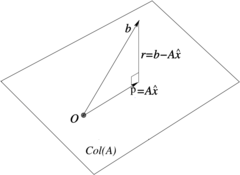
Therefore, the vector ${\textstyle \mathbf {p} =P_{_{A}}\mathbf {b} }$ is the orthogonal projection of ${\textstyle \mathbf {b} }$ onto the column space of ${\textstyle A}$, as illustrated in Figure 1. Additionally, relation (3) defines a well posed problem (a consistent linear problem), with unique solution, since ${\textstyle A}$ is full rank. This unique solution is the least squares solution obtained from the normal equations.

Figure 1: $\operatorname {Col} (A)$ is orthogonal to the minimum residual ${\widehat {\mathbf {r} }}=\mathbf {b} -A\,{\widehat {\mathbf {x} }}=\mathbf {b} -P_{_{A}}\mathbf {b}$.

2.3 Instability of the normal equations method

The normal equations approach is a very simple procedure to solve the linear least squares problem. It is the most used approach in the scientific and engineering community, and very popular in statistical software. However, it must be used with precaution, specially when the design matrix ${\textstyle A}$ is ill-conditioned (or it is rank deficient) and finite precision arithmetic, in digital conventional devices, is employed. In order to understand this phenomenon, it is convenient to show an example and then discuss the results.

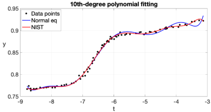
Example 2: The National Institute of Standards and Technology (NIST) is a branch of the U.S. Department of Commerce responsible for establishing national and international standards. NIST maintains reference data sets for use in the calibration and certification of statistical software. On its website [10] we can find the Filip data set, which consists of 82 observations of a variable ${\textstyle y}$ for different ${\textstyle t}$ values. The aim is to model this data set using a 10th-degree polynomial. This is part of exercise 5.10 in Cleve Molers' book [11]. For this problem we have ${\textstyle m=82}$ data points ${\textstyle (t_{i},{\hat {y}}_{i})}$, and we want to compute ${\textstyle n=11}$ coefficients ${\textstyle c_{j}}$ for the 10th-degree polynomial. The ${\textstyle m\times n}$ design matrix ${\textstyle A}$ has coefficients ${\textstyle a_{ij}=t_{i}^{j-1}}$. In order to given an idea of the complexity of this matrix, we observe that its minimum coefficient is 1 and its maximum coefficient is a bit greater than ${\textstyle 2.7\times 10^{9}}$, while its condition number is ${\textstyle \kappa (A)\approx {\mathcal {O}}(10^{15})}$. The matrix of the normal equations, ${\textstyle A^{T}A}$, is a much smaller matrix of size ${\textstyle n\times n}$, but more singular, since its minimum and maximum coefficients (in absolute value) are close to 82 and ${\textstyle 5.1\times 10^{19}}$, respectively, with a very high condition number ${\textstyle \kappa (A^{T}A)\approx {\mathcal {O}}(10^{30})}$. The matrix of the normal equations is highly ill-conditioned in this case because there are some clusters of data points very close to each other with almost identical ${\textstyle t_{i}}$ values. The computed coefficients ${\textstyle {\widehat {c}}_{j}}$ using the normal equations are shown in Table 1, along with the certified values provided by NIST. The NIST certified values were found solving the normal equations, but with multiple precision of 500 digits (which represents an idealization of what would be achieved if the calculations were made without rounding error). Our calculated values differ significantly from those of NIST, even in the sign, the relative difference ${\textstyle \Vert {\widehat {\mathbf {c} }}-\mathbf {c} _{nist}\Vert /\Vert \mathbf {c} _{nist}\Vert }$ is about 118${\textstyle \%}$. This dramatic difference is mainly because we are using finite arithmetic with 16-digit standard IEEE double precision, and solving the normal equations with the Cholesky factorization yields a relative error amplified proportionately to the product of the condition number times the machine epsilon. The computed residual keeps reasonable, though. Figure 2 shows Filip data along with the certified curve and our computed curve. The difference is most visible at the extremes, where our computed curve shows some pronounced oscillations.

Table. 1 Comparison of numerical results with the NIST's certified values.

Polynomial coefficients	NIST ${\textstyle (\times 10^{3})}$	Normal equations ${\textstyle (\times 10^{2})}$
${\textstyle {\widehat {c}}_{1}}$	-1.467489614229800	3.397167285217155
${\widehat {c}}_{2}$	-2.772179591933420	5.276500833542165
${\widehat {c}}_{3}$	-2.316371081608930	3.545138197108058
${\widehat {c}}_{4}$	-1.127973940983720	1.345510235823048
${\widehat {c}}_{5}$	-0.354478233703349	0.316966659871258
${\widehat {c}}_{6}$	-0.075124201739376	0.047864845714924
${\widehat {c}}_{7}$	-0.010875318035534	0.004604461850533
${\widehat {c}}_{8}$	-0.001062214985889	0.000269285797556
${\widehat {c}}_{9}$	-0.000067019115459	0.000008526963608
${\widehat {c}}_{10}$	-0.000002467810783	0.000000107514812
${\widehat {c}}_{11}$	-0.000000040296253	0.000000000044407
Relative difference	0	118${\textstyle \%}$
Norm of residual	0.028400823094900	0.041260859317660

Figure 2:' Computed polynomial curve along with NISTs certified one.

3 Orthogonal projections and the QR factorization

The previous numerical results for solving a least square problem have shown instability for the normal equations approach, when the design matrix is ill-conditioned. However the normal equations approach usually yields good results when the problem is of moderate size as well as well-conditioned. For the cases where the design matrix is ill-conditioned the QR factorization method is an excellent alternative. The SVD factorization is convenient when the design matrix is rank deficient, as will be discussed below.

3.1 The QR factorization

We begin with the following theorem in reference [9].

Theorem 1: Each ${\textstyle A\in \mathbb {C} ^{m\times n}(m\geq n)}$ of full rank has a unique reduced ${\textstyle QR}$ factorization ${\textstyle A={\widehat {Q}}{\widehat {R}}}$ with ${\textstyle r_{jj}>0}$. For simplicity we keep the discussion for the case ${\textstyle A\in \mathbb {R} ^{m\times n}}$. In this case ${\textstyle {\widehat {Q}}}$ is the same size than ${\textstyle A}$ and ${\textstyle {\widehat {R}}\in \mathbb {R} ^{n\times n}}$ is upper triangular. Actually this factorization is a matrix version of the Gram-Schmidt orthogonalization algorithm. More precisely, let ${\textstyle \mathbf {a} _{1},\mathbf {a} _{2},\ldots ,\mathbf {a} _{n}\in \mathbb {R} ^{m}}$ be the linear independent column vectors of ${\textstyle A}$

$A=\left[{\begin{array}{cccc}|&|&&|\\\mathbf {a} _{1}&\mathbf {a} _{2}&\cdots &\mathbf {a} _{n}\\|&|&&|\end{array}}\right],$

then the orthonormal vectors ${\textstyle \mathbf {q} _{1}}$, ${\textstyle \mathbf {q} _{2}}$, ... , ${\textstyle \mathbf {q} _{n}}$ en ${\textstyle \mathbb {R} ^{m}}$ obtained from the Gram-Schmidt orthogonalization gives the following matrix

${\widehat {Q}}=\left[{\begin{array}{cccc}|&|&&|\\\mathbf {q} _{1}&\mathbf {q} _{2}&\cdots &\mathbf {q} _{n}\\|&|&&|\end{array}}\right],$

which has the same column space that ${\textstyle A}$. These vectors are constructed sequentially, starting with ${\textstyle \mathbf {q} _{1}=\mathbf {a} _{1}/\Vert \mathbf {a} _{1}\Vert }$, and they satisfy

$\mathbf {q} _{j}={\dfrac {\mathbf {v} _{j}}{\|\mathbf {v} _{j}\|_{2}}}\quad {\hbox{con}}\quad \mathbf {v} _{j}=\mathbf {a} _{j}-(\mathbf {q} _{1}^{T}\mathbf {a} _{j})\mathbf {q} _{1}-\ldots -(\mathbf {q} _{j-1}^{T}\mathbf {a} _{j})\,\mathbf {q} _{j-1}=\mathbf {a} _{j}-\sum _{i=1}^{j-1}(\mathbf {q} _{i}^{T}\mathbf {a} _{j})\,\mathbf {q} _{i}\,\quad 1\leq j\leq n.$

Using the notation ${\textstyle r_{ij}\equiv \mathbf {q} _{i}^{T}\mathbf {a} _{j}\,}$ for ${\textstyle i>j}$ and ${\textstyle r_{jj}=\|\mathbf {v} _{j}\|_{2}}$, we obtain

${\textstyle \mathbf {q} _{1}}$	=	${\dfrac {\mathbf {a} _{1}}{r_{11}}}\,,$
$\mathbf {q} _{2}$	=	${\dfrac {\mathbf {a} _{2}-r_{12}\,\mathbf {q} _{1}}{r_{22}}}\,,$
$\mathbf {q} _{n}$	=	${\dfrac {\mathbf {a} _{n}-\sum _{i=1}^{n-1}r_{in}\,\mathbf {q} _{i}}{r_{nn}}}\,.$

and

$\mathbf {a} _{1}$	=	$r_{11}\,\mathbf {q} _{1}\,,$
$\mathbf {a} _{2}$	=	$r_{12}\,\mathbf {q} _{1}+r_{22}\,\mathbf {q} _{2}\,,$
$\mathbf {a} _{n}$	=	$r_{1n}\,\mathbf {q} _{1}+r_{2n}\,\mathbf {q} _{2}+\cdots +r_{nn}\,\mathbf {q} _{n}\,.$

This set of equations leads to the so called reduced $QR$ factorization:

$A$

=

$\left[{\begin{array}{cccc}|&|&&|\\\mathbf {a} _{1}&\mathbf {a} _{2}&\cdots &\mathbf {a} _{n}\\|&|&&|\end{array}}\right]=\left[{\begin{array}{cccc}|&|&&|\\\mathbf {q} _{1}&\mathbf {q} _{2}&\cdots &\mathbf {q} _{n}\\|&|&&|\end{array}}\right]\,\left[{\begin{array}{cccc}r_{11}&r_{12}&\ldots &r_{1n}\\0&r_{22}&\ldots &r_{2n}\\\vdots &&\ddots &\vdots \\0&0&\ldots &r_{nn}\end{array}}\right]={\widehat {Q}}\,{\widehat {R}}$.

This factorization allows another way to solve the overdetermined system ${\textstyle A\mathbf {x} =\mathbf {b} }$, that arise in linear least square problems. The key property is that ${\textstyle {\widehat {Q}}^{T}{\widehat {Q}}=I_{n}}$, where ${\textstyle I_{n}}$ is the identity matrix of size ${\textstyle n\times n}$. Then

${\widehat {Q}}{\widehat {R}}\,\mathbf {x} =\mathbf {b} \quad {\hbox{is equivalent to}}\quad {\widehat {R}}\,\mathbf {x} ={\widehat {Q}}^{T}\mathbf {b} ,$

(4)

and this triangular system is solved easily using backward substitution. Furthermore, the obtained solution is the least squares solution, since the following set of relations are equivalent

${\widehat {R}}\mathbf {x} ={\widehat {Q}}^{T}\mathbf {b} ,\quad {\widehat {Q}}{\widehat {R}}\mathbf {x} ={\widehat {Q}}{\widehat {Q}}^{T}\mathbf {b} ,\quad A\mathbf {x} =P_{_{\widehat {Q}}}\mathbf {b} ,\quad A\mathbf {x} =P_{_{A}}\mathbf {b} ,$

where the projection matrices satisfy ${\textstyle P_{_{\widehat {Q}}}\mathbf {b} =P_{_{A}}\mathbf {b} }$ because the column space of ${\textstyle A}$ is equal to the column space of ${\textstyle {\widehat {Q}}}$.

A complete ${\textstyle QR}$ factorization of ${\textstyle A}$ goes further by adding ${\textstyle m-n}$ orthonormal columns to ${\textstyle {\widehat {Q}}}$, and adding ${\textstyle m-n}$ rows of zeros to ${\textstyle {\widehat {R}}}$, obtaining an orthogonal matrix ${\textstyle Q\in \mathbb {R} ^{m\times m}}$ and an upper triangular matrix ${\textstyle R\in \mathbb {R} ^{m\times n}}$ as shown in Figure 3. In the complete factorization the additional columns ${\textstyle \mathbf {q} _{j}}$, ${\textstyle j=n+1,\ldots ,m}$, are orthogonal to the column space of ${\textstyle A}$. Of course, the matrix ${\textstyle Q}$ is an orthogonal matrix, since 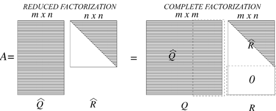${\textstyle Q^{T}Q=I_{m}}$, so ${\textstyle Q^{-1}=Q^{T}}$.

Figure 3: The reduced and complete $QR$ factorizations of $A$

Theorem 2: Any matrix ${\textstyle A\in \mathbb {R} ^{m\times n}}$ (${\textstyle m\geq n}$) has a complete factorization ${\textstyle QR}$, given by ${\textstyle A=QR}$ with ${\textstyle Q\in \mathbb {R} ^{m\times m}}$ an orthogonal matrix and ${\textstyle R\in \mathbb {R} ^{m\times n}}$ an upper triangular matrix.

Warning. The Gram-Schmidt algorithm is numerically unstable (sensitive to rounding errors). Stabilization methods can be used by changing the order in which the operations are performed. Fortunately, there is an stable algorithm to compute the ${\textstyle QR}$ factorization which relies on Householder reflections.

3.2 Householder reflections

A Householder reflection is a linear transformation with matrix ${\textstyle H}$, which is constructed from a given fixed vector ${\textstyle \mathbf {x} }$ in a Euclidean space ${\textstyle \mathbb {R} ^{p}}$ (${\textstyle p\geq 2}$), seeking its reflected vector to be ${\textstyle H\,\mathbf {x} =||\mathbf {x} ||\,\mathbf {e} _{1}=(||\mathbf {x} ||,0,\ldots ,0)^{T}}$, as shown in Figure 4.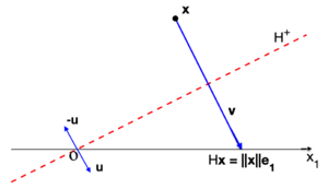

Figure 4: Householder reflection with vector $\mathbf {v} =||\mathbf {x} ||\,\mathbf {e} _{1}-\mathbf {x}$.

This reflection reflects on a hyperplane ${\textstyle H^{+}}$ with normal unitary vector ${\textstyle \mathbf {u} }$, and is given by

$H=I-2\mathbf {u} \mathbf {u} ^{T},\quad {\hbox{with}}\quad \mathbf {u} ={\frac {\mathbf {v} }{\Vert \mathbf {v} \Vert }},\quad \mathbf {v} =\|\mathbf {x} \|\,\mathbf {e} _{1}-\mathbf {x} ,$

(5)

where the outer (or external) product ${\textstyle \mathbf {u} \mathbf {u} ^{T}}$ gives rise to a rank one symmetric matrix. We emphasize that, given the vector ${\textstyle \mathbf {x} }$, the projection ${\textstyle H}$ performs the following transformation

$\mathbf {x} =\left[{\begin{array}{c}x_{1}\\x_{2}\\\vdots \\x_{p}\end{array}}\right]\quad \longmapsto \quad H\,\mathbf {x} =\left[{\begin{array}{c}||\mathbf {x} ||\\0\\\vdots \\0\end{array}}\right]=\|\mathbf {x} \|\,\mathbf {e} _{1}.$

This matrix is a symmetric orthogonal matrix, i.e. it satisfies ${\textstyle H^{T}H=I_{p}}$, ${\textstyle H^{T}=H}$.

Matrix ${\textstyle A}$ is transformed into an upper triangular matrix ${\textstyle R}$ by successively applying Householder matrix transformations ${\textstyle H_{k}}$

$H_{n}\cdots H_{2}\,H_{1}\,A=R.$

Each ${\textstyle H_{k}}$ matrix is chosen to introduce zeros below the diagonal in the ${\textstyle k}$-th column. For example, for a matrix ${\textstyle A}$ of ${\textstyle m\times n=5\times 3}$, the ${\textstyle H_{k}}$ operations are applied as shown below:

$\overbrace {\underbrace {\left[\!\!{\begin{array}{ccc}a_{11}&a_{12}&a_{13}\\a_{21}&a_{22}&a_{23}\\a_{31}&a_{32}&a_{33}\\a_{41}&a_{42}&a_{43}\\a_{51}&a_{52}&a_{53}\end{array}}\!\!\right]} _{A}} ^{A}\rightarrow \overbrace {\underbrace {\left[\!\!{\begin{array}{ccc}a_{11}^{(1)}&a_{12}^{(1)}&a_{13}^{(1)}\\0&a_{22}^{(1)}&a_{23}^{(1)}\\0&a_{32}^{(1)}&a_{33}^{(1)}\\0&a_{42}^{(1)}&a_{43}^{(1)}\\0&a_{52}^{(1)}&a_{53}^{(1)}\end{array}}\!\!\right]} _{H_{1}A}} ^{A^{(1)}}\rightarrow \overbrace {\underbrace {\left[\!\!{\begin{array}{ccc}a_{11}^{(1)}&a_{12}^{(1)}&a_{13}^{(1)}\\0&a_{22}^{(2)}&a_{23}^{(2)}\\0&0&a_{33}^{(2)}\\0&0&a_{43}^{(2)}\\0&0&a_{5}^{(2)}\end{array}}\!\!\right]} _{H_{2}H_{1}A}} ^{A^{(2)}}\rightarrow \overbrace {\underbrace {\left[\!\!{\begin{array}{ccc}a_{11}^{(1)}&a_{12}^{(1)}&a_{13}^{(1)}\\0&a_{22}^{(2)}&a_{23}^{(2)}\\0&0&a_{33}^{(3)}\\0&0&0\\0&0&0\end{array}}\!\!\right]} _{H_{3}H_{2}H_{1}A}} ^{R}\,,$

where each ${\textstyle H_{k}\in \mathbb {R} ^{m\times m}}$ is of the form

$H_{k}=\left[{\begin{array}{cc}I_{k}&\mathbb {O} ^{T}\\\mathbb {O} &H\end{array}}\right]\,,$

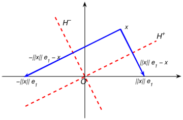
which is a symmetric orthogonal matrix (see [12] for more details), ${\textstyle I_{k}}$ is the identity matrix of size ${\textstyle k\times k}$, and ${\textstyle \mathbb {O} }$ is the zero matrix of size ${\textstyle (m-k)\times k}$. Actually, for any vector ${\textstyle \mathbf {x} }$ there are two Householder refletions, as shown in Figure 5, and each Householder matrix ${\textstyle H}$ is constructed with the election ${\textstyle \mathbf {v} =\operatorname {sign} (x_{1})\|\mathbf {x} \|\,\mathbf {e} _{1}+\mathbf {x} }$. It is evident that this election allows ${\textstyle \|\mathbf {v} \|}$ to never be smaller than ${\textstyle \|\mathbf {x} \|}$, avoiding cancellation by subtraction when dividing by ${\textstyle \Vert \mathbf {v} \Vert }$ to find ${\textstyle \mathbf {u} }$ in (5), thus ensuring stability of the method.

Figure 5: Two Huoseholder reflections, constructed from $\mathbf {x}$.

The above process is called Householder triangularization [13], and currently it is the most widely used method for finding the ${\textstyle QR}$ factorization. There are two procedures to construct the reflection matrices: Givens rotations and Householder reflections. Here we have described only Householder reflections. For further insight, we refer the reader to [14], [12] and [9].

We may compute the factorization ${\textstyle A={\widehat {Q}}{\widehat {R}}}$, with ${\textstyle {\widehat {Q}}=(H_{n}\cdots H_{2}H_{1})^{T}}$. However, if we are interested only in the solution of the least squares problem, we do not have to compute explicitly either matrices ${\textstyle H_{k}}$ or ${\textstyle {\widehat {Q}}}$. We just find the factor ${\textstyle R}$ and store it in the same memory space occupied by ${\textstyle A}$, and ${\textstyle {\widehat {Q}}^{T}\mathbf {b} }$ and store it in the same memory location occupied by ${\textstyle \mathbf {b} }$. At the end, we solve the triangular system with backward substitution, as shown bellow.

Householder triangularization algorithm for solving $A\,\mathbf {x} =\mathbf {b}$ with ${\textstyle QR}$

${\textstyle {\hbox{for }}k=1,\ldots ,n}$ ** Triangularization **

${\textstyle .\quad \mathbf {x} =A(k:m,\,k)}$

${\textstyle .\quad \mathbf {v} =sign(x_{1})\|\mathbf {x} \|\,\mathbf {e} _{1}+\mathbf {x} }$

${\textstyle .\quad \mathbf {v} =\mathbf {v} /\|\mathbf {v} \|}$

${\textstyle .\quad A(k:m,\,k:n)=A(k:m,\,k:n)-2\mathbf {v} \,(\mathbf {v} ^{T}\,A(k:m,\,k:n))}$

${\textstyle .\quad \mathbf {b} (k:m)=\mathbf {b} (k:m)-2\mathbf {v} (\mathbf {v} ^{T}\,\mathbf {b} (k:m))}$

${\textstyle {\hbox{end}}}$

${\textstyle \mathbf {x} (n)=\mathbf {b} (n)/A(n,n)}$ ** Backward sustitution **

${\textstyle {\hbox{for }}k=n-1:-1:1}$

${\textstyle \vdots \quad \mathbf {x} (k)=(\mathbf {b} (k)-A(k,k+1:n)\cdot \mathbf {b} (k+1:n))/A(k,k)}$

${\textstyle {\hbox{end}}}$

Notation. We have used the MATLAB notation for arrays. For instance, ${\textstyle \mathbf {x} =A(k:m,\,k)}$ represents the vector constructed with coefficients ${\textstyle a_{ik}}$, ${\textstyle k\leq i\leq m}$ and ${\textstyle k}$ fixed; ${\textstyle A(k:m,\,k:n)}$ represents the submatrix with coefficients ${\textstyle \left\{a_{ij}\right\}_{i=k,j=k}^{m,n}}$; ${\textstyle \mathbf {b} (k:m)}$ represents the subvector ${\textstyle \left\{b_{i}\right\}_{i=k}^{m}}$.

The most important steps in the previous algorithm are the last two lines in the ** Triangularization ** loop. The main idea is that it is not necessary to construct ${\textstyle H}$ to compute a product ${\textstyle H\,\mathbf {y} }$, since

$H\,\mathbf {y} =(I-2\mathbf {u} \mathbf {u} ^{T})\mathbf {y} =\mathbf {y} -\mathbf {u} (\mathbf {u} ^{T}\mathbf {y} )\quad {\hbox{with}}\quad \mathbf {u} ={\frac {\mathbf {v} }{\Vert \mathbf {v} \Vert }},$

so we only need the vectors ${\textstyle \mathbf {v} }$ and ${\textstyle \mathbf {y} }$ at each step of the process. Numerical results are shown in Section 6.

4 The singular value decomposition (SVD)

4.1 Symmetrizing

The key idea to achieving the SVD of a matrix ${\textstyle A}$ is symmetrizing. That is, if ${\textstyle A\in \mathbb {R} ^{m\times n}}$, we can consider the symmetric positive semidefinite matrices ${\textstyle A^{T}A\in \mathbb {R} ^{n\times n}}$ and ${\textstyle A\,A^{T}\in \mathbb {R} ^{m\times m}}$. By the spectral theorem for symmetric matrices, these matrices are diagonalizable. For instance, if ${\textstyle \lambda _{1},\ldots ,\lambda _{n}}$ are the eigenvalues of ${\textstyle A^{T}A}$ with orthonormal eigenvectors ${\textstyle \mathbf {v} _{1},\mathbf {v} _{2},\ldots ,\mathbf {v} _{n}}$, then

$A^{T}A=V\,D\,V^{T},\quad {\hbox{with}}\quad V=\left[{\begin{array}{cccc}{\Big \vert }&{\Big \vert }&&{\Big \vert }\\\mathbf {v} _{1}&\mathbf {v} _{2}&\cdots &\mathbf {v} _{n}\\{\Big \vert }&{\Big \vert }&&{\Big \vert }\\\end{array}}\right],\quad D=\left[{\begin{array}{cccc}\lambda _{1}&0&\cdots &0\\0&\lambda _{2}&\cdots &0\\\vdots &\vdots &\ddots &\vdots \\0&0&\cdots &\lambda _{n}\end{array}}\right].$

Each eigenvalue ${\textstyle \lambda _{j}}$ is real and non-negative, because

$A^{T}A\,\mathbf {v} _{j}=\lambda _{j}\,\mathbf {v} _{j}\quad \Rightarrow \quad \mathbf {v} _{j}^{T}A^{T}A\,\mathbf {v} _{j}=\lambda _{j}\,\mathbf {v} _{j}^{T}\mathbf {v} _{j}\quad \Rightarrow \quad \lambda _{j}={\frac {\Vert A\,\mathbf {v} _{j}\Vert ^{2}}{\Vert \mathbf {v} _{j}\Vert ^{2}}}\geq 0.$

(6)

Therefore, we can order the eigenvalues. Without loss of generality, we assume that

$\lambda _{1}\geq \lambda _{2}\geq \cdots \geq \lambda _{n}\geq 0.$

We remark that some eigenvalues may be repeated. Furthermore, each eigenvalue ${\textstyle \lambda _{j}}$ of ${\textstyle A^{T}A}$ is also an eigenvalue of ${\textstyle A\,A^{T}}$ since

$A^{T}A\,\mathbf {v} _{j}=\lambda \mathbf {v} _{j}\quad \Rightarrow \quad (A\,A^{T})A\,\mathbf {v} _{j}=\lambda _{j}\,A\mathbf {v} _{j}.$

4.2 Reduced SVD

We have found that matrices ${\textstyle A^{T}A}$ and ${\textstyle A\,A^{T}}$ have the same eigenvalues ${\textstyle \lambda _{1}\geq \lambda _{2}\geq \ldots \geq \lambda _{n}\geq 0}$ with corresponding eigenvectors

$\mathbf {v} _{1},\mathbf {v} _{2},\ldots ,\mathbf {v} _{n}\in \mathbb {R} ^{n}\quad {\hbox{and}}\quad A\mathbf {v} _{1},A\mathbf {v} _{2},\ldots ,A\mathbf {v} _{n}\in \mathbb {R} ^{m},$

respectively. The eigenvectors ${\textstyle \mathbf {v} _{j}}$ of ${\textstyle A^{T}A}$ are orthonormal. However, the eigenvectors of ${\textstyle A\,A^{T}}$ are only orthogonal (${\textstyle (A\mathbf {v} _{i})^{T}A\mathbf {v} _{j}=\mathbf {v} _{i}^{T}A^{T}A\mathbf {v} _{j}=\mathbf {v} _{i}^{T}\lambda _{j}\mathbf {v} _{j}=\lambda _{j}\delta _{ij}}$), so we normalize them to get an orthonormal set ${\textstyle \mathbf {u} _{1},\ldots ,\mathbf {u} _{n}}$ in ${\textstyle \mathbb {R} ^{m}}$

$\mathbf {u} _{j}={\frac {A\,\mathbf {v} _{j}}{\Vert A\,\mathbf {v} _{j}\Vert }}={\frac {A\,\mathbf {v} _{j}}{\left(\lambda _{j}\right)^{1/2}}},\quad j=1,2,\ldots ,n.$

(7)

Definition 1: Non-negative values

$\sigma _{1}={\sqrt {\lambda _{1}}}\geq \sigma _{2}={\sqrt {\lambda _{2}}}\geq \ldots \geq \sigma _{n}={\sqrt {\lambda _{n}}}\geq 0,$

are called the singular values of the matrix ${\textstyle A}$. Therefore, according to (7), the following relationship is obtained between the two sets of orthonormal vectors ${\textstyle \left\{\mathbf {u} _{1},\ldots ,\mathbf {u} _{n}\right\}\subset \mathbb {R} ^{m}}$ and ${\textstyle \left\{\mathbf {v} _{1},\ldots ,\mathbf {v} _{n}\right\}\subset \mathbb {R} ^{n}}$:

$A\,\mathbf {v} _{j}=\sigma _{j}\mathbf {u} _{j},\quad j=1,2,\ldots ,n.$

(8)

These relationships can be expressed as the matrix product:

$A\,\left[{\begin{array}{cccc}\vert &\vert &&\vert \\\mathbf {v} _{1}&\mathbf {v} _{2}&\cdots &\mathbf {v} _{n}\\\vert &\vert &&\vert \end{array}}\right]=\left[{\begin{array}{cccc}\vert &\vert &&\vert \\\sigma _{1}\mathbf {u} _{1}&\sigma _{2}\mathbf {u} _{2}&\cdots &\sigma _{n}\mathbf {u} _{n}\\\vert &\vert &&\vert \end{array}}\right],$

which leads to

$A=\underbrace {\left[{\begin{array}{cccc}{\Big \vert }&{\Big \vert }&&{\Big \vert }\\\mathbf {u} _{1}&\mathbf {u} _{2}&\cdots &\mathbf {u} _{n}\\{\Bigg \vert }&{\Bigg \vert }&&{\Bigg \vert }\\\end{array}}\right]} \underbrace {\left[{\begin{array}{cccc}\sigma _{1}&0&\cdots &0\\0&\sigma _{2}&\cdots &0\\\vdots &\vdots &\ddots &\vdots \\0&0&\cdots &\sigma _{n}\end{array}}\right]} \underbrace {\left[{\begin{array}{ccc}{\hbox{-----}}&\mathbf {v} _{1}^{T}&{\hbox{ -----}}\\{\hbox{ -----}}&\mathbf {v} _{2}^{T}&{\hbox{ -----}}\\&\vdots &\\{\hbox{ -----}}&\mathbf {v} _{n}^{T}&{\hbox{ -----}}\end{array}}\right].}$ (9) ${\widehat {U}}(m\times n)\qquad {\widehat {\Sigma }}(n\times n)V^{T}(n\times n)$

This factorization can also be expressed as sum of rank one matrices:

$A=\sigma _{1}\mathbf {u} _{1}\mathbf {v} _{1}^{T}+\sigma _{2}\mathbf {u} _{2}\mathbf {v} _{2}^{T}+\cdots +\sigma _{n}\mathbf {u} _{n}\mathbf {v} _{n}^{T},\quad {\hbox{with}}\quad \sigma _{1}\geq \sigma _{2}\geq \cdots \geq \sigma _{n}\geq 0.$

(10)

Note. In the matrix equation ${\textstyle AV={\widehat {U}}{\widehat {\Sigma }}}$ or ${\textstyle A={\widehat {U}}{\widehat {\Sigma }}V^{T}}$, the matrix ${\textstyle {\widehat {U}}}$ is a rectangular matrix of size ${\textstyle m\times n}$ with orthonormal columns in ${\textstyle \mathbb {R} ^{m}}$, ${\textstyle {\widehat {\Sigma }}}$ is an ${\textstyle n\times n}$ diagonal matrix with singular values, and ${\textstyle V}$ is an ${\textstyle n\times n}$ orthogonal matrix (i.e. ${\textstyle V^{-1}=V^{T}}$). The reduced SVD is also valid for matrices with complex entries or coefficients, but now ${\textstyle V}$ is Hermitian, so ${\textstyle V^{*}}$ (the complex conjugate) replaces ${\textstyle V^{T}}$ in the matrix factorization. For the interested reader, reference [15] is an extraordinary paper that surveys the contributions of five mathematicians who were responsible for establishing the existence of the SVD and developing its theory.

4.3 Full SVD

In most applications, the reduced SVD decomposition is employed. However, in textbooks and many publications, the `full' SVD decomposition is used. The reduced and full SVD are the same for ${\textstyle m=n}$. We illustrate two cases: ${\textstyle m>n}$ and ${\textstyle m<n}$.

• Case $m>n$: the columns of the matrix ${\widehat {U}}$ do not form a basis of ${\textstyle \mathbb {R} ^{m}}$. We augment ${\textstyle {\widehat {U}}\in \mathbb {R} ^{m\times n}}$ to an orthogonal matrix ${\textstyle U\in \mathbb {R} ^{m\times m}}$ by adding ${\textstyle m-n}$ orthonormal columns and replacing ${\textstyle {\widehat {\Sigma }}\in R^{n\times n}}$ by ${\textstyle \Sigma \in \mathbb {R} ^{m\times n}}$ adding ${\textstyle m-n}$ null rows ${\textstyle {\widehat {\Sigma }}}$:

$A=\underbrace {\left[\!\!{\begin{array}{ccccccc}{\Bigg \vert }&{\Bigg \vert }&&{\Bigg \vert }&{\Bigg \vert }&&{\Bigg \vert }\\\mathbf {u} _{1}&\mathbf {u} _{2}&\cdots &\mathbf {u} _{n}&\mathbf {u} _{n+1}&\cdots &\mathbf {u} _{m}\\{\Bigg \vert }&{\Bigg \vert }&&{\Bigg \vert }&{\Bigg \vert }&&{\Bigg \vert }\\\end{array}}\!\!\right]} \underbrace {\left[\!\!{\begin{array}{cccc}\sigma _{1}&0&\cdots &0\\0&\sigma _{2}&\cdots &0\\\vdots &\vdots &\ddots &\vdots \\0&0&\cdots &\sigma _{n}\\0&0&\cdots &0\\\vdots &\vdots &\ddots &\vdots \\0&0&\cdots &0\end{array}}\!\!\right]} \underbrace {\left[\!\!{\begin{array}{ccc}{\hbox{-----}}&\mathbf {v} _{1}^{T}&{\hbox{ -----}}\\{\hbox{ -----}}&\mathbf {v} _{2}^{T}&{\hbox{ -----}}\\&\vdots &\\{\hbox{ -----}}&\mathbf {v} _{n}^{T}&{\hbox{ -----}}\end{array}}\!\!\right].}$ (11) $U(m\times m)\qquad \Sigma (m\times n)V^{T}(n\times n)$

• Case $m<n$: the reduced decomposition is of the form ${\textstyle A=U{\widehat {\Sigma }}{\widehat {V}}^{T}}$. The rows of ${\textstyle {\widehat {V}}^{T}}$ does not form a basis of ${\textstyle \mathbb {R} ^{n}}$ so we must add ${\textstyle n-m}$ orthonormal rows to obtain an orthogonal matrix ${\textstyle V^{T}}$ and adding ${\textstyle n-m}$ null columns to ${\textstyle {\widehat {\Sigma }}}$ to get ${\textstyle \Sigma }$:

$A=\underbrace {\left[\!\!{\begin{array}{cccc}{\Bigg \vert }&{\Bigg \vert }&&{\Bigg \vert }\\\mathbf {u} _{1}&\mathbf {u} _{2}&\cdots &\mathbf {u} _{m}\\{\Bigg \vert }&{\Bigg \vert }&&{\Bigg \vert }\end{array}}\!\!\right]} \underbrace {\left[\!\!{\begin{array}{ccccccc}\sigma _{1}&0&\cdots &0&0&\cdots &0\\0&\sigma _{2}&\cdots &0&0&\cdots &0\\\vdots &\vdots &\ddots &\vdots &\vdots &\vdots &\vdots \\0&0&\cdots &\sigma _{m}&0&\cdots &0\\\end{array}}\!\!\right]} \underbrace {\left[\!\!{\begin{array}{ccc}{\hbox{-----}}&\mathbf {v} _{1}^{T}&{\hbox{ -----}}\\{\hbox{ -----}}&\mathbf {v} _{2}^{T}&{\hbox{ -----}}\\&\vdots &\\{\hbox{ -----}}&\mathbf {v} _{m}^{T}&{\hbox{ -----}}\\{\hbox{ -----}}&\mathbf {v} _{m+1}^{T}&{\hbox{ -----}}\\{\hbox{ -----}}&\vdots &{\hbox{ -----}}\\{\hbox{ -----}}&\mathbf {v} _{n}^{T}&{\hbox{ -----}}\\\end{array}}\!\!\right].}$ (12) $U(m\times m)\qquad \Sigma (m\times n)V^{T}(n\times n)$

The previous results are summarized in the following theorem.

Theorem 3: Every matrix ${\textstyle A\in \mathbb {R} ^{m\times n}}$ (${\textstyle \mathbb {C} ^{m\times n}}$, in the complex case) has a singular value decomposition of the form

$A=U\Sigma V^{T},\quad (A=U\Sigma V^{*},{\hbox{in the complex case}})$

(13)

with the orthogonal matrices ${\textstyle U}$, ${\textstyle V}$ (or unitary, in the complex case), and the matrix ${\textstyle \Sigma }$ as indicated in the previous development.

4.4 Computing the SVD

As stated in [9] (Lecture 23), the SVD of ${\textstyle A\in \mathbb {C} ^{m\times n}}$ ${\textstyle (m>n)}$, ${\textstyle A=U\,\Sigma \,V^{*}}$ is related to the eigenvalue decomposition of the covariance matrix ${\textstyle A^{*}A=V\,\Sigma ^{*}\Sigma \,V^{*}}$ and mathematically it may be calculated doing the following:

1. Form ${\textstyle A^{*}A}$;
2. Compute the eigenvalue decomposition ${\textstyle A^{*}A=V\,\Lambda \,V^{*}}$;
3. Let ${\textstyle \Sigma }$ be the non negative diagonal square root of ${\textstyle \Lambda }$;
4. Solve the system ${\textstyle U\,\Sigma =A\,V}$ for unitary ${\textstyle U}$ (e.g. via ${\textstyle QR}$ factorization).

But the problem with this strategy is that the algorithm is not stable, mainly because it relies on the covariance matrix ${\textstyle A^{*}A}$, which we have found before in the normal equations for least squares problems. Additionally, the eigenvalue problem in general is very sensitive to numerical perturbations in computer’s finite precision arithmetic

An alternative stable way to compute the SVD is to reduce it to an eigenvalue problem by considering a ${\textstyle 2m\times 2m}$ Hermitian matrix and the corresponding eigenvalue system.

$H=\left[{\begin{array}{cc}0&A^{*}\\A&0\end{array}}\right]\quad \Longrightarrow \quad H\left[{\begin{array}{c}V\\U\end{array}}\right]=\left[{\begin{array}{c}V\,\Sigma \\U\,\Sigma \end{array}}\right],$

since ${\textstyle A=U\Sigma V^{*}}$ implies ${\textstyle A\,V=U\Sigma }$ and ${\textstyle A^{*}U=V\,\Sigma }$. Thus the singular values of ${\textstyle A}$ are the absolute values of the eigenvalues of ${\textstyle H}$, and the singular vectors of ${\textstyle A}$ can be extracted from the eigenvectors of ${\textstyle H}$, which can be done in an stable way, contrary to the previous strategy. This Hermitian eigenvalue problems are usually solved by a two-phase computation: first reduce the matrix to tridiagonal form, then diagonalize the tridiagonal matrix. The reduction is done by similarity unitary transformations, so the diagonal matrix contains the information about the singular values.

Actually, this strategy has been standard for computing the SVD since the work of Golub and Kahan in the 1960s [16]. The method involves in phase 1 applying Householder reflections alternately from the left and right of the matrix to reduce it to an upper bidiagonal form. In phase 2, the SVD of the bidiagonal matrix is determined with a variant of the QR algorithm. More recently, divide-and-conquer algorithms [17] have become the standard approach for computing the SVD of dense matrices in practice. These strategies overcome the computational difficulties associated with ill-conditioned or rank-deficient matrices during the SVD calculations.

4.5 Least squares with SVD

Most of the software environments, like MATLAB and Phyton, incorporate very efficient algorithms and state of the art tools related to SVD. So, using those routines provide reasonable accurate results in most of the cases.

Concerning linear least squares problems, we know that this often leads to an inconsistent overdetermined system ${\textstyle A\mathbf {x} =\mathbf {b} }$ with ${\textstyle A\in \mathbb {R} ^{m\times n}}$, ${\textstyle m\geq n}$. Thus, we seek the minimum of the residual ${\textstyle \mathbf {r} =\mathbf {b} -A\mathbf {x} }$. We know that if ${\textstyle A}$ is of full rank ${\textstyle r=n}$, then ${\textstyle A^{T}A}$ is positive definite symmetric and the least squares solution is given by

${\widehat {\mathbf {x} }}=\left(A^{T}A\right)^{-1}A^{T}\mathbf {b} .$

Via SVD, ${\textstyle A=U\Sigma V^{T}}$, and using that ${\textstyle V^{-1}=V^{T}}$, ${\textstyle U^{-1}=U^{T}}$, ${\textstyle \Sigma ^{T}\Sigma }$ invertible, we have

$\left(A^{T}A\right)^{-1}A^{T}=\left(V\Sigma ^{T}U^{T}U\Sigma V^{T}\right)^{-1}V\,\Sigma ^{T}U^{T}=V\,\left(\Sigma ^{T}\Sigma \right)^{-1}\Sigma ^{T}U^{T}=V\Sigma ^{\dagger }U^{T}=A^{\dagger },$

and the least squares solution is given by

${\widehat {\mathbf {x} }}=A^{\dagger }\mathbf {b} .$

(14)

What is remarkable is that the solution given by (14) is still valid, even if ${\textstyle A}$ is rank deficient. The following formal definition of the pseudoinverse corroborate our claim.

Definition 2: Let ${\textstyle A=U\Sigma V^{T}}$ a real ${\textstyle m\times n}$ matrix with rank ${\textstyle r\leq n}$, then its pseudoinverse is the ${\textstyle n\times m}$ matrix, denoted by ${\textstyle A^{\dagger }}$, given by

$A^{\dagger }=V\Sigma ^{\dagger }U^{T}\quad {\hbox{with}}\quad \Sigma ^{\dagger }={\hbox{diag}}(1/\sigma _{1},\ldots ,1/\sigma _{r},0,\ldots ,0)\in \mathbb {R} ^{n\times m}.$

(15)

With this definition ${\textstyle A^{\dagger }}$ is well defined and it has the same size as ${\textstyle A^{T}}$. If ${\textstyle A}$ is full rank, then ${\textstyle A^{\dagger }}$ is called the left inverse of ${\textstyle A}$ since ${\textstyle A^{\dagger }A=I_{n}}$, and ${\textstyle P_{_{A}}=AA^{\dagger }}$ defines the projection onto the column space of ${\textstyle A}$. When ${\textstyle A}$ is an invertible square matrix ${\textstyle A^{\dagger }=A^{-1}}$.

Fitting data to a polynomial curve. Given the point set ${\textstyle (t_{1},{\hat {y}}_{1}),\ldots ,(t_{m},{\hat {y}}_{m})}$. The algorithm for calculating ${\textstyle {\widehat {\mathbf {x} }}\in \mathbb {R} ^{n+1}}$, with the coefficients of the polynomial of degree ${\textstyle n}$, consists of the following steps:

1. Form the ${\textstyle m\times (n+1)}$ design matrix ${\textstyle A}$, with coefficients ${\textstyle a_{ij}=t_{i}^{j-1}}$.
2. Compute the SVD of ${\textstyle A=U\,\Sigma V^{T}}$. Actually, the reduced SVD, ${\textstyle A={\widehat {U}}{\widehat {\Sigma }}V^{T}}$, is sufficient.
3. Calculate the generalized inverse ${\textstyle A^{\dagger }=V\,\Sigma ^{\dagger }U^{T}}$.
4. Calculate ${\textstyle {\widehat {\mathbf {x} }}=A^{\dagger }\mathbf {b} }$, with ${\textstyle \mathbf {b} =\{{\hat {y}}_{j}\}_{j=1}^{m}}$ being the vector of observations.

In Section 5 we present numerical results and compare them with the results obtained with ${\textstyle QR}$ and normal equations algorithms.

5 Numerical comparisons of QR and SVD

As before we consider the Filip data set, which consists of 82 observations of a variable ${\textstyle y}$ for different ${\textstyle t}$ values. The aim is to model these data set using a 10th-degree polynomial, using both, the QR factorization and SVD, to solve the associated least squares problem. In Section 2 we gave a description of the data and showed numerical results with the normal equations approach. Here we use the QR algorithm with Householder reflections, introduced in Section 3, and the SVD, described in Section 4.

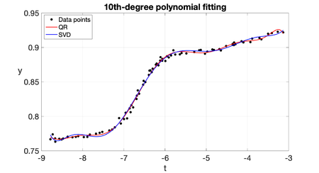
Table 2 shows the coefficient values of the polynomial obtained with both algorithms. The coefficients obtained with the QR algorithm are very close to the certified values of NIST (shown in Table 1), while the coefficients obtained with SVD are far from the certified ones, with two or three orders of magnitude apart and different signs for most of them. In fact, the relative difference ${\textstyle \Vert {\widehat {\mathbf {c} }}-\mathbf {c} _{nist}\Vert /\Vert \mathbf {c} _{nist}\Vert }$ of the coefficients obtained with the stable QR is insignificant, while the relative difference is as high as ${\textstyle 100\%}$ when the SVD is employed. However, the polynomial obtained with the SVD shows that the data still fit fairly well to the obtained curve, as shown in Figure 6. Again, the main differences between the accurate curve (red line) with respect to the less accurate (blue line) is more evident at the left and right extremes of the interval.

A better measure for accuracy is the norm of the residual ${\textstyle \Vert \mathbf {b} -A\,{\widehat {\mathbf {x} }}\Vert }$, since the algorithms are designed to minimize this quantity. We observe that the residual obtained with the QR algorithm is very close to the certified one (shown in Figure 2) and, surprisingly this residual is slightly lower than the certified one, while the residual obtained with the SVD is higher than the certified one but lower than the one obtained with the normal equations. So, we conclude that the best method for this particular problem is QR, followed by SVD and the less accurate is obtained with the normal equations.

Table. 2 Comparison of polynomial coefficients: QR and SVD.

Polynomial coefficients	QR ${\textstyle (\times 10^{3})}$	SVD
${\textstyle {\widehat {c}}_{1}}$	-1.467489624841714	8.443047022531269
${\widehat {c}}_{2}$	-2.772179612867669	1.364997532790476
${\widehat {c}}_{3}$	-2.316371099847143	-5.350747822573923
${\widehat {c}}_{4}$	-1.127973950228995	-3.341901399544638
${\widehat {c}}_{5}$	-0.354478236724762	-0.406458058717373
${\widehat {c}}_{6}$	-0.075124202404921	0.257727453320758
${\widehat {c}}_{7}$	-0.010875318135669	0.119771677097139
${\widehat {c}}_{8}$	-0.001062214996057	0.023140894524175
${\widehat {c}}_{9}$	-0.000067019116127	0.002403995388431
${\widehat {c}}_{10}$	-0.000002467810808	0.000131618846926
${\widehat {c}}_{11}$	-0.000000040296253	0.000002990001355
Relative difference	$7.68\times 10^{-7}\%$	100${\textstyle \%}$
Norm of residual	0.028210838088578	0.032726981836403

Figure 6: Computed polynomial curve with QR and SVD.

6 Neural network approach

Finally, we present a neural network (NN) framework to address the same fitting problem analyzed in the preceding sections. While NNs have historically been less common than classical methods, they have recently emerged as powerful tools across numerous scientific disciplines. Our goal is to develop a NN that can be used together with the known data for curve fitting. If we have ${\textstyle m}$ observations

$(t_{1},\,{\hat {y}}_{1}),\,(t_{2},\,{\hat {y}}_{2}),\ldots ,\,(t_{m},\,{\hat {y}}_{m})\,,$

(16)

where ${\textstyle {\hat {y}}_{i}}$, ${\textstyle i=1,2,\ldots ,\,m}$, are measurements of ${\textstyle y(t_{i})}$. The idea is to model ${\textstyle y(t)}$ as a NN of the form:

$y(t)\approx {\widetilde {y}}(t,\mathbf {W} ,\mathbf {b} ),$

(17)

where ${\textstyle \mathbf {W} }$ and ${\textstyle \mathbf {b} }$ are two sets of parameters of the neural network, which must be determined. This NN model consists of an input layer, ${\textstyle L}$ hidden layers, each one containing ${\textstyle N_{\ell }}$ neurons, and an additional output layer. The received input signal propagates through the network from the input layer to the output layer, through the hidden layers. When the signals arrive in each node, an activation function ${\textstyle \phi :\mathbb {R} \to \mathbb {R} }$ is used to produce the node output [18,19,20]. Neural networks with many layers (two or more) are called multi-layer neural networks.

Example 3: The model corresponding to a neural network with a single hidden layer consisting of five neurons, each activated by the hyperbolic tangent function, and a scalar output obtained through a linear combination of the hidden activations, can be expressed as

${\widetilde {y}}(t,\mathbf {W} ,\mathbf {b} )=W^{2}\phi (W^{1}t+b^{1})+b^{2},$

where ${\textstyle \phi (x)=\tanh(x)}$. Explicitly, in this case, the neural network can be written as a functional representation of the input ${\textstyle x}$ in the following form:

${\widetilde {y}}(t,\mathbf {W} ,\mathbf {b} )=\,W_{1}^{2}\tanh(W_{1}^{1}t+b_{1}^{1})+W_{2}^{2}\tanh(W_{2}^{1}t+b_{2}^{1})+$ $W_{3}^{2}\tanh(W_{3}^{1}t+b_{3}^{1})+W_{4}^{2}\tanh(W_{4}^{1}t+b_{4}^{1})+$ $W_{5}^{2}\tanh(W_{5}^{1}t+b_{5}^{1})+b^{2}.$

Hence, the complete model involves ${\textstyle 16}$ unknown parameters, which entirely determine the behavior of the neural network. The unknown parameters are optimized using an appropriate optimization algorithm (e.g., gradient descent) based on the given training dataset (16). The goal is to minimize a loss function that quantifies the discrepancy between the network's predictions and the true target values, which is described below.

Remark 2: It is known that any continuous, non-constant function mapping ${\textstyle \mathbb {R} }$ to ${\textstyle \mathbb {R} }$ can be approximated arbitrarily well by a multilayer neural network, see [21,22,23]. This result establishes the expressive power of feedforward neural networks. Specifically, it shows that even a network with a single hidden layer, containing a sufficient number of neurons and an appropriate activation function, can approximate any continuous function on compact subsets of ${\textstyle \mathbb {R} }$.

6.1 General NN architecture

In this work, the neural network is described in terms of the input ${\textstyle t\in \mathbb {R} }$, the output ${\textstyle {\widetilde {y}}\in \mathbb {R} }$, and an input-to-output mapping ${\textstyle t\mapsto {\widetilde {y}}}$. For any hidden layer ${\textstyle \ell }$, we consider the pre-activation ${\textstyle T^{\ell }\in \mathbb {R} ^{N_{\ell }}}$ and post-activation ${\textstyle Y^{\ell }\in \mathbb {R} ^{N_{\ell {+1}}}}$ vectors as

$T^{\ell }(t)=\left[T_{1}^{\ell }(t),\dots ,T_{N_{\ell }}^{\ell }(t)\right]^{T}\qquad \mathrm {and} \qquad Y^{\ell }(t)=\left[Y_{1}^{\ell }(t),\dots ,Y_{N_{\ell }{+1}}^{\ell }(t)\right]^{T},$

(18)

respectively. Thus, the activation in the ${\textstyle \ell }$-th hidden layer of the network for ${\textstyle j=1,\dots ,N_{\ell {+1}},}$ is given by [24]:

$\displaystyle Y_{j}^{\ell }(t)=b_{j}^{\ell }+\sum _{k=1}^{N_{\ell }}W_{k}^{\ell }\,\,T_{k}^{\ell }(t),\qquad \ell =1,\dots ,L,$

(19)

where

$T_{k}^{1}(t)=t,\qquad T_{k}^{\ell }(t)=\phi (Y_{k}^{\ell {-1}}(t)),\qquad \ell =2,\dots ,L,$

(20)

for ${\textstyle k=1,\dots ,N_{\ell }}$. Here, ${\textstyle W_{k}^{\ell }}$ and ${\textstyle b^{\ell }}$ are the weights and bias parameters of layer ${\textstyle \ell }$. Activation functions ${\textstyle \phi }$ must be chosen such that the differential operators can be readily and robustly evaluated using reverse mode automatic differentiation [25]. Throughout this work, we have been using relatively simple feedforward neural networks architectures with hyperbolic tangent and sigmoidal activation functions. Results show that these functions are robust for the proposed formulation. It is important to remark that as more layers and neurons are incorporated into the NN the number of parameters significantly increases. Thus the optimization process becomes less efficient.

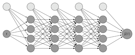
Figure 7 shows an example of the computational graph representing a NN as described in equations (18)–(20). When one node's value is the input of another node, an arrow goes from one to another. In this particular example, we have

${\hbox{layers}}={\big (}N_{\ell }{\big )}_{\ell =1}^{L+2}=(1,4,4,4,4,1).$

That is, the total number of hidden layers is ${\textstyle 4}$. The first entry corresponds to the input layer (${\textstyle \ell =1}$) and contains a single neuron. The next four entries correspond to the hidden layers, each one with ${\textstyle N_{\ell }=4}$ neurons. Finally, the last layer is the output layer and contains one neuron, corresponding to a single solution value. Bias is also considered (light grey nodes), there is a bias node in each layer, which has a value equal to the unit and is only connected to the nodes of the next layer. Although, the number of nodes for each layer can be different; the same number has been employed in this paper for simplicity.

Figure 7: Neural network with 4 hidden layers, one input and one output.

6.2 Optimization Algorithm

The parameters ${\textstyle \mathbf {W} }$ and ${\textstyle \mathbf {b} }$ in (17) are determined using a finite set of training points ${\textstyle \{t_{i},{\hat {y}}_{i}\}_{i=1}^{m}}$ corresponding to the dataset in (16). Here, ${\textstyle m}$ denotes the number of training points, which can be arbitrarily selected. The parameters are estimated by minimizing the mean squared error (MSE) loss

$E={\frac {1}{N_{u}}}\sum _{i=1}^{N_{u}}\left|{\widetilde {y}}(t_{i},\mathbf {W} ,\mathbf {b} )-{\hat {y}}_{i}\right|^{2},$

(21)

where ${\textstyle E}$ represents the error over the training dataset ${\textstyle \{t_{i},{\hat {y}}_{i}\}_{i=1}^{m}}$. The neural network defined in (18)–(20) is trained iteratively, updating the neuron weights by minimizing the discrepancy between the target values ${\textstyle {\hat {y}}_{i}}$ and the outputs ${\textstyle {\widetilde {y}}(t_{i},\mathbf {W} ,\mathbf {b} )}$.

Formally, the optimization problem can be written as

$\min _{[\mathbf {W} ,\mathbf {b} ]}E([\mathbf {W} ,\mathbf {b} ]),$

(22)

where the vector ${\textstyle [\mathbf {W} ,\mathbf {b} ]}$ collects all unknown weights and biases. Several optimization algorithms can be employed to solve the minimization problem (21) and (22), and the final performance strongly depends on the residual loss achieved by the chosen method. In this work, the optimization process is performed using gradient-based algorithms, such as Stochastic Gradient Descent (SGD) or Adam [26]. These methods iteratively adjust the network parameters in the direction that minimizes the loss function. Starting from an initial guess ${\textstyle [\mathbf {W} ^{0},\mathbf {b} ^{0}]}$, the algorithm generates a sequence of iterates ${\textstyle [\mathbf {W} ^{1},\mathbf {b} ^{1}],\,[\mathbf {W} ^{2},\mathbf {b} ^{2}],\,[\mathbf {W} ^{3},\mathbf {b} ^{3}],\ldots ,}$ converging to a (local) minimizer as the stopping criterion is satisfied.

The required gradients are computed efficiently using automatic differentiation [27], which applies the chain rule to propagate derivatives through the computational graph. In practice, this process is known as backpropagation [28]. All computations were carried out in Python using Pytorch [26], a widely used and well-documented open-source library for machine learning.

6.3 Results

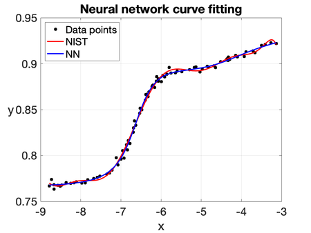
To illustrate the capability of the NN, we consider the same curve-fitting problem based on the Filip dataset, which consists of 82 observations of a variable ${\textstyle y}$ at different values of ${\textstyle t}$. The computed solution is shown in Figures 8 and 9. The predicted values of ${\textstyle y}$ are obtained by training all the parameters of a five-layer neural network: the first layer contains a single neuron, while each hidden layer consists of twenty neurons. The hyperbolic tangent and sigmoidal activation functions are used throughout the network. It is worth noting that the NN solution closely resembles the one obtained using a 10th-degree polynomial fit (NIST). Therefore, this example shows its potential for generalization and robustness in more challenging scenarios.

Figure 8: NN solution with the hyperbolic tangent as activation function.

Figure 9: NN solution with the sigmoidal as activation function.

7 Conclusions

Fitting a curve to a given set of data is one of the most simple of the so called ill-posed problems. This is an example of a broad set of problems called least squares problems. This simple problem contains many of the ingredients, both theoretical and computational, of modern challenge and complex problems that are of great importance in computational modelling and applications, specially when computer solutions are obtained using finite precision machines. Commonly there is no `best computational algorithm' for general problems, but for a particular problem, like the one considered in this article, we can compare results obtained with different approaches or algorithms.

It is clear that the best fit to a 10th-degree polynomial is obtained with the QR algorithm, as it produces the smallest residual when compared to algorithms based on the normal equations and SVD. It is noteworthy that each method yields entirely different coefficients for this polynomial. Not only the sign of the coefficients but also the scale of the values differ drastically. These results demonstrate that even simple ill-posed problems must be studied and numerically solved with extreme care, employing stable state-of-the-art algorithms and tools that avoid the accumulation of rounding errors due to the finite arithmetic precision of computers.

Concerning the neural network approach, we obtained qualitatively excellent numerical results. The resulting fitted curve is smooth and provides an accurate representation of the data, and it appears to offer a slightly improved approximation when compared to the QR-based fit, while maintaining sufficient flexibility to capture the overall behavior. These results suggest that the multi-layer neural networks constitute an effective and robust framework for curve fitting. Is the NN approach better than the QR algorithm for curve fitting? Again, this general question depends of what you are looking for. But if you are able to construct with NN a 10th-degree polynomial that fits the given experimental data, then you are able to answer this particular question. A diligent reader may put their hands on the problem in order to give an answer.

Acknowledgements. We would like to express our sincere gratitude to the Department of Mathematics at Universidad Autónoma Metropolitana–Iztapalapa for their valuable support of this research work. The authors also gratefully acknowledge partial support from the Secretaría de Ciencia, Humanidades, Tecnología e Innovación (Secihti) through the Investigadores e Investigadoras por México program and the Ciencia de Frontera Project No. CF-2023-I-2639.

BIBLIOGRAPHY

[1] A. M. Legendre. (1805) "Nouvelles methodes pour la determination des orbites des cometes". Courcier

[2] C. F. Gauss. (1963) "Theory of the Motion of the Heavenly Bodies Moving about the Sun in Conic Sections". Dover

[3] Åke Björck. (1996) "Numerical Methods for Least Squares Problems". SIAM

[4] Mansfield Merriman. (1877) "Note on the History of the Method of Least Squares", Volume 4. The Analyst 5 140–143

[5] C. F. Gauss. (1995) "Theory of the Combination of Observations Least Subject to Errors. Part I, Part II, Supplement". SIAM

[6] Yves Nievergelt. (2000) "A tutorial history of least squares with applications to astronomy and geodesy", Volume 121. Journal of Computational and Applied Mathematics 37–72

[7] P. Businger and G. H. Golub. (1965) "Linear least squares solutions by Householder transformations", Volume 7. Numerische Mathematik 269–276

[8] G. H. Golub and C. Reinsch. (1970) "Singular value decomposition and least squares solutions", Volume 14. Numerische Mathematik 403–420

[9] Lloyd N. Trefethen and David Bau III. (1997) "Numerical Linear Algebra". SIAM

[10] "Statistical Reference Datasets: Filip Data" https://www.itl.nist.gov/div898/strd/lls/data/Filip.shtml

[11] Cleve B. Moler. (2004) "Numerical Computing with MATLAB". SIAM

[12] L. Héctor Juárez. (2025) "Resultados relevantes del álgebra lineal en modelos y aplicaciones", Volume 16. Revista Metropolitana de Matemáticas Mixba'al 1

[13] A. S. Householder. (1958) "A Class of Methods for Inverting Matrices", Volume 6. Journal of the Society for Industrial and Applied Mathematics 2 189–195

[14] Gene H. Golub and Charles F. Van Loan. (1983) "Matrix Computations". The Johns Hopkins University Press

[15] G. W. Stewart. (1993) "On the Early History of the Singular Value Decomposition", Volume 35. SIAM Review 4 551–566

[16] G. H. Golub and W. Kahan. (1965) "Calculating the singular values and pseudo-inverse of a matrix", Volume 2. SIAM Journal on Numerical Analysis 2 205–224

[17] Y. Nakatsukasa and N. Higham. (2013) "Stable and efficient spectral divide and conquer algorithms for the symmetric eigenvalue decomposition and the SVD", Volume 35. SIAM Journal on Scientific Computing 3 A1325–A1349

[18] S. Marsland. (2015) "Machine Learning: An Algorithmic Perspective". CRC Press

[19] S. Pattanayak. (2017) "Pro Deep Learning with TensorFlow: A Mathematical Approach to Advanced Artificial Intelligence in Python". Apress

[20] G. Zaccone and R. Karim. (2018) "Deep Learning with TensorFlow: Explore Neural Networks and Build Intelligent Systems with Python". Packt Publishing Ltd

[21] G. Cybenko. (1989) "Approximation by superpositions of a sigmoidal function", Volume 2. Mathematics of Control, Signals and Systems 4 303–314

[22] K. Hornik and M. Stinchcombe and H. White. (1989) "Multilayer feedforward networks are universal approximators", Volume 2. Neural Networks 5 359–366

[23] A. Pinkus. (1999) "Approximation theory of the MLP model in neural networks", Volume 8. Acta Numerica 143–195

[24] C. Michoski and M. Milosavljevic and T. Oliver and D. Hatch. (2019) "Solving irregular and data-enriched differential equations using deep neural networks"

[25] D. A. Fournier and H. J. Skaug and J. Ancheta and J. Ianelli and A. Magnusson and M. N. Maunder and A. Nielsen and J. Sibert. (2012) "AD Model Builder: Using automatic differentiation for statistical inference of highly parameterized complex nonlinear models", Volume 27. Optimization Methods & Software 2 233–249

[26] . (2025) "PyTorch" https://pytorch.org

[27] A. G. Baydin and B. A. Pearlmutter and A. A. Radul and J. M. Siskind. (2015) "Automatic differentiation in machine learning: a survey"

[28] M. A. Nielsen. (2015) "Neural Networks and Deep Learning". Determination Press