m (teste) (Tag: Visual edit) |
m (teste) (Tag: Visual edit) |
||
| Line 410: | Line 410: | ||
For each <math display="inline">\bar{\theta }\in \left[ -\frac{\pi }{2},\frac{\pi }{2} \right)\times \left[ -\frac{\pi }{2},\frac{\pi }{2} \right)</math>, three other frequency components <math>{{\phi }_{h}}\left( \theta ,x \right)</math> with <math display="inline">\theta \in [-\pi ,\pi )\times [-\pi ,\pi )</math> coincide in <math>G_{2h}</math> with <math>{{\phi }_{h}}\left( \bar{\theta },x \right)</math> and are not visible in <math>G_{2h}</math> . Therefore, the low- and high-frequency components are defined as follows: | For each <math display="inline">\bar{\theta }\in \left[ -\frac{\pi }{2},\frac{\pi }{2} \right)\times \left[ -\frac{\pi }{2},\frac{\pi }{2} \right)</math>, three other frequency components <math>{{\phi }_{h}}\left( \theta ,x \right)</math> with <math display="inline">\theta \in [-\pi ,\pi )\times [-\pi ,\pi )</math> coincide in <math>G_{2h}</math> with <math>{{\phi }_{h}}\left( \bar{\theta },x \right)</math> and are not visible in <math>G_{2h}</math> . Therefore, the low- and high-frequency components are defined as follows: | ||
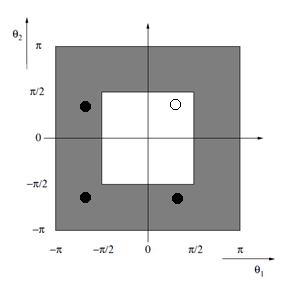
| − | <math>\varphi</math> is a low-frequency component<math>\Leftrightarrow \theta \in {{T}^{low}}=\left[ -\frac{\pi }{2},\frac{\pi }{2} \right)\times \left[ -\frac{\pi }{2},\frac{\pi }{2} \right)</math><math>\varphi</math> is a high-frequency component<math>\theta \in {{T}^{high}}=\left[ -\pi ,\pi \right)\times \left[ -\pi ,\pi \right)\backslash \left[ -\frac{\pi }{2},\frac{\pi }{2} \right)\times \left[ -\frac{\pi }{2},\frac{\pi }{2} \right)</math>. See Fig. 2. | + | <math>\varphi</math> is a low-frequency component<math>\Leftrightarrow \theta \in {{T}^{low}}=\left[ -\frac{\pi }{2},\frac{\pi }{2} \right)\times \left[ -\frac{\pi }{2},\frac{\pi }{2} \right)</math> |
| + | |||
| + | <math>\varphi</math> is a high-frequency component<math>\theta \in {{T}^{high}}=\left[ -\pi ,\pi \right)\times \left[ -\pi ,\pi \right)\backslash \left[ -\frac{\pi }{2},\frac{\pi }{2} \right)\times \left[ -\frac{\pi }{2},\frac{\pi }{2} \right)</math>. See Fig. 2. | ||
<div class="center" style="width: auto; margin-left: auto; margin-right: auto;"> | <div class="center" style="width: auto; margin-left: auto; margin-right: auto;"> | ||
| Line 458: | Line 460: | ||
|} | |} | ||
| − | where | + | where <math>\hat{K}_{h}^{2h}(\theta )</math> is given by Eq. (19) and <math>{{\hat{S}}_{h}}(\theta )</math> is a 4x4 matrix and represents <math>{{S}_{h}}(\theta )</math>. |
Let it be | Let it be | ||
| Line 492: | Line 494: | ||
For the bilinear prolongation operator, <math>\overset{\tilde{\ }}{\mathop{I_{2h}^{h}}}\,\left( {{\theta }^{\alpha }} \right)=(1+\cos {{\bar{\theta }}_{1}})(1+\cos {{\bar{\theta }}_{2}})</math> and for the 7-point prolongation operator, <math>\overset{\tilde{\ }}{\mathop{I_{2h}^{h}}}\,\left( {{\theta }^{\alpha }} \right)=\left( 1+\cos {{{\bar{\theta }}}_{1}}+\cos {{{\bar{\theta }}}_{2}}+\cos ({{{\bar{\theta }}}_{1}}-{{{\bar{\theta }}}_{2}}) \right)</math> [10]. | For the bilinear prolongation operator, <math>\overset{\tilde{\ }}{\mathop{I_{2h}^{h}}}\,\left( {{\theta }^{\alpha }} \right)=(1+\cos {{\bar{\theta }}_{1}})(1+\cos {{\bar{\theta }}_{2}})</math> and for the 7-point prolongation operator, <math>\overset{\tilde{\ }}{\mathop{I_{2h}^{h}}}\,\left( {{\theta }^{\alpha }} \right)=\left( 1+\cos {{{\bar{\theta }}}_{1}}+\cos {{{\bar{\theta }}}_{2}}+\cos ({{{\bar{\theta }}}_{1}}-{{{\bar{\theta }}}_{2}}) \right)</math> [10]. | ||
| − | In order to perform the LFA using the <math display="inline">\mbox{ILU}</math> solver, the eigen-functions of <math>{{L}_{h}}</math>, | + | In order to perform the LFA using the <math display="inline">\mbox{ILU}</math> solver, the eigen-functions of <math>{{L}_{h}}</math>, <math>{{\overset{\hat{\ }}{\mathop{L}}\,}_{h}}</math>, <math>{{\overset{\hat{\ }}{\mathop{U}}\,}_{h}}</math> and <math>{{R}_{h}}</math> are given by |
| − | + | ||
| − | <math>{{\overset{\hat{\ }}{\mathop{L}}\,}_{h}}</math>, | + | |
| − | + | ||
| − | <math>{{\overset{\hat{\ }}{\mathop{U}}\,}_{h}}</math> and | + | |
| − | + | ||
| − | <math>{{R}_{h}}</math> are given by | + | |
{| class="formulaSCP" style="width: 100%;margin: 1em auto 0.1em auto;width: 100%;text-align: center;" | {| class="formulaSCP" style="width: 100%;margin: 1em auto 0.1em auto;width: 100%;text-align: center;" | ||
| Line 517: | Line 513: | ||
{| style="text-align: center; margin:auto;width: 100%;" | {| style="text-align: center; margin:auto;width: 100%;" | ||
|- | |- | ||
| − | | <math>{{S}_{h}}\phi (\theta ,x)={{\overset{\tilde{\ }}{\mathop{S}}\,}_{h}}\phi (\theta ,x)</math>, | + | | <math>{{S}_{h}}\phi (\theta ,x)={{\overset{\tilde{\ }}{\mathop{S}}\,}_{h}}\phi (\theta ,x)</math>, <math>-\pi \le \theta <\pi </math>, |
| − | <math>-\pi \le \theta <\pi </math>, | + | |
|} | |} | ||
| style="text-align: center;width: 5px;text-align: right;white-space: nowrap;" |(24) | | style="text-align: center;width: 5px;text-align: right;white-space: nowrap;" |(24) | ||
| Line 541: | Line 536: | ||
In this work, the anisotropic diffusion equation was solved using 7-point ILU solver in different directions. Several restriction operators and two prolongation operators were employed. It is proposed an algorithm that presents the lowest asymptotic convergence factor values and the lowest computational cost for the multigrid method. | In this work, the anisotropic diffusion equation was solved using 7-point ILU solver in different directions. Several restriction operators and two prolongation operators were employed. It is proposed an algorithm that presents the lowest asymptotic convergence factor values and the lowest computational cost for the multigrid method. | ||
| − | Eq. (2) was assessed for | + | Eq. (2) was assessed for<math>\varepsilon ={{10}^{\kappa }}</math> and <math>\varepsilon ={{10}^{-\kappa }}</math>, with <math>\kappa \in \Kappa =\{0,\,\,1,\,\,2,\,\,3,\,\,4,\,\,5,\,\,6,\,\,7\}</math>. When <math>\varepsilon ={{10}^{\kappa }}</math> or <math>\varepsilon ={{10}^{-\kappa }}</math> in this work, there is symmetric anisotropy. For instance, <math>\varepsilon ={{10}^{2 }}</math> is an anisotropy symmetric to <math>\varepsilon ={{10}^{-2}}</math>. |
Section 4.1 presents the convergence analysis by means of LFA. Only the optimum components obtained via LFA will be used in the complexity analysis in section 4.2. | Section 4.1 presents the convergence analysis by means of LFA. Only the optimum components obtained via LFA will be used in the complexity analysis in section 4.2. | ||
| Line 547: | Line 542: | ||
===4.1. Convergence Analysis=== | ===4.1. Convergence Analysis=== | ||
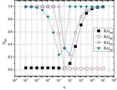
| − | Fig. 3 depicts | + | Fig. 3 depicts <math>{{\rho }_{loc}}</math> , given by Eq. (22), with <math display="inline">\mbox{ILU}</math> in the EN, NE, ES, SE directions, FW restriction, bilinear prolongation, number of inner iterations <math>v=2</math>,<math>\varepsilon ={{10}^{\kappa }}</math>and <math>\varepsilon ={{10}^{-\kappa }}</math>, with <math>\kappa \in K</math>. |
<div class="center" style="width: auto; margin-left: auto; margin-right: auto;"> | <div class="center" style="width: auto; margin-left: auto; margin-right: auto;"> | ||
[[Image:draft_Vassoler Rutz_344011008-image153.jpeg|390px]] </div> | [[Image:draft_Vassoler Rutz_344011008-image153.jpeg|390px]] </div> | ||
| − | Figure 3: | + | Figure 3: <math>{{\rho }_{loc}}</math> ''versus'' anisotropy coefficients ( [[Image:draft_Vassoler Rutz_344011008-image154.png|12px]] ) with <math display="inline">\mbox{ILU}</math> in different directions. |
It is noticed that for [[Image:draft_Vassoler Rutz_344011008-image156.png|66px]] , <math display="inline">{\mbox{ILU}}_{\mbox{EN}}</math> has a good performance and for | It is noticed that for [[Image:draft_Vassoler Rutz_344011008-image156.png|66px]] , <math display="inline">{\mbox{ILU}}_{\mbox{EN}}</math> has a good performance and for | ||
| Line 564: | Line 559: | ||
For the analyses presented below, tests were carried out using only the solvers that had the best performances in the previous analysis. | For the analyses presented below, tests were carried out using only the solvers that had the best performances in the previous analysis. | ||
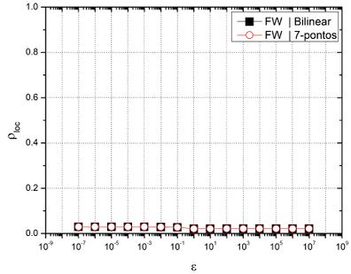
| − | Fig. 4 presents | + | Fig. 4 presents <math>{{\rho }_{loc}}</math> using as solvers, <math display="inline">{\mbox{ILU}}_{\mbox{EN}}</math> for [[Image:draft_Vassoler Rutz_344011008-image156.png|66px]] and <math display="inline">{\mbox{ILU}}_{\mbox{NE}}</math> for [[Image:draft_Vassoler Rutz_344011008-image158.png|42px]] ; [[Image:draft_Vassoler Rutz_344011008-image164.png|36px]] ; FW restriction; 7-point and bilinear prolongation; [[Image:draft_Vassoler Rutz_344011008-image141.png|48px]] and [[Image:draft_Vassoler Rutz_344011008-image151.png|54px]] , with [[Image:draft_Vassoler Rutz_344011008-image165.png|42px]] . |
<div class="center" style="width: auto; margin-left: auto; margin-right: auto;"> | <div class="center" style="width: auto; margin-left: auto; margin-right: auto;"> | ||
| Line 571: | Line 566: | ||
<span id='_GoBack'></span> | <span id='_GoBack'></span> | ||
| − | Figure 4: | + | Figure 4: <math>{{\rho }_{loc}}</math> ''versus'' anisotropy coefficients ( [[Image:draft_Vassoler Rutz_344011008-image154.png|12px]] ) with different interpolation operators. |
It is observed that the restriction|prolongation combinations FW|bilinear and FW|7-points had a good performance ( [[Image:draft_Vassoler Rutz_344011008-image160.png|48px]] ) and presented very similar convergence factors. | It is observed that the restriction|prolongation combinations FW|bilinear and FW|7-points had a good performance ( [[Image:draft_Vassoler Rutz_344011008-image160.png|48px]] ) and presented very similar convergence factors. | ||
| Line 577: | Line 572: | ||
Bilinear prolongation operator was used in the following analysis as it is easy to program and demands fewer memory resources. The asymptotic convergence factors were compared with different restriction operators. | Bilinear prolongation operator was used in the following analysis as it is easy to program and demands fewer memory resources. The asymptotic convergence factors were compared with different restriction operators. | ||
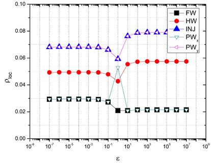
| − | Fig. 5 presents'' '' | + | Fig. 5 presents'' ''<math>{{\rho }_{loc}}</math> using as solvers, <math display="inline">{\mbox{ILU}}_{\mbox{EN}}</math> for [[Image:draft_Vassoler Rutz_344011008-image156.png|66px]] and <math display="inline">{\mbox{ILU}}_{\mbox{NE}}</math> for [[Image:draft_Vassoler Rutz_344011008-image158.png|42px]] ; [[Image:draft_Vassoler Rutz_344011008-image164.png|36px]] ; FW, HW, INJ, <math display="inline">{\mbox{PW}}_\mbox{x}</math> and <math display="inline">{\mbox{PW}}_\mbox{y}</math> restriction; bilinear prolongation; [[Image:draft_Vassoler Rutz_344011008-image141.png|48px]] and [[Image:draft_Vassoler Rutz_344011008-image151.png|54px]] , with [[Image:draft_Vassoler Rutz_344011008-image165.png|42px]] . |
<div class="center" style="width: auto; margin-left: auto; margin-right: auto;"> | <div class="center" style="width: auto; margin-left: auto; margin-right: auto;"> | ||
[[Image:draft_Vassoler Rutz_344011008-image171.jpeg|414px]] </div> | [[Image:draft_Vassoler Rutz_344011008-image171.jpeg|414px]] </div> | ||
| − | Figure 5: | + | Figure 5: <math>{{\rho }_{loc}}</math> ''versus'' anisotropy coefficients ( [[Image:draft_Vassoler Rutz_344011008-image154.png|12px]] ) with different restriction operators. |
| − | Fig. 5 shows that for [[Image:draft_Vassoler Rutz_344011008-image172.png|54px]] and [[Image:draft_Vassoler Rutz_344011008-image173.png|48px]] , with [[Image:draft_Vassoler Rutz_344011008-image165.png|42px]] (symmetric anisotropies), [[Image:draft_Vassoler Rutz_344011008-image174.png|24px]] presents very similar values. It is noted that for anisotropic problems ( [[Image:draft_Vassoler Rutz_344011008-image175.png|36px]] ), the lowest values for | + | Fig. 5 shows that for [[Image:draft_Vassoler Rutz_344011008-image172.png|54px]] and [[Image:draft_Vassoler Rutz_344011008-image173.png|48px]] , with [[Image:draft_Vassoler Rutz_344011008-image165.png|42px]] (symmetric anisotropies), [[Image:draft_Vassoler Rutz_344011008-image174.png|24px]] presents very similar values. It is noted that for anisotropic problems ( [[Image:draft_Vassoler Rutz_344011008-image175.png|36px]] ), the lowest values for <math>{{\rho }_{loc}}</math> are achieved with FW and <math display="inline">{\mbox{PW}}_\mbox{x}</math> restriction, which present very similar values. |
| − | Based on the results shown, it is proposed Algorithm 1, which combines ILU solver in different directions with FW and <math display="inline">{\mbox{PW}}_\mbox{x}</math> restrictions. The algorithm will be presented now. The abbreviation '''REST''', used in the algorithm, represents any of the restrictions (FW or <math display="inline">{\mbox{PW}}_\mbox{x}</math> ) previously defined. | + | Based on the results shown, it is proposed Algorithm 1, which combines ILU solver in different directions with FW and <math display="inline">{\mbox{PW}}_\mbox{x}</math> restrictions. The algorithm will be presented now. The abbreviation '''REST''', used in the algorithm, represents any of the restrictions (FW or <math display="inline">{\mbox{PW}}_\mbox{x}</math>) previously defined. |
Algorithm1: | Algorithm1: | ||
| Line 608: | Line 603: | ||
___________________________________________________________________________ | ___________________________________________________________________________ | ||
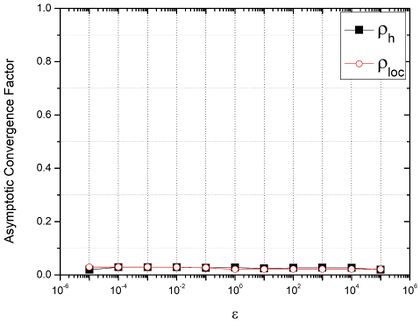
| − | Next, it is presented the asymptotic convergence factor | + | Next, it is presented the asymptotic convergence factor <math>{{\rho }_{loc}}</math>, calculated via LFA, and the empiric asymptotic convergence factor [[Image:draft_Vassoler Rutz_344011008-image185.png|18px]] , for different anisotropy coefficients. |
Fig. 6 shows Algorithm 1 with '''REST''' <math display="inline">={\mbox{PW}}_\mbox{x}</math> , [[Image:draft_Vassoler Rutz_344011008-image164.png|36px]] and bilinear prolongation. | Fig. 6 shows Algorithm 1 with '''REST''' <math display="inline">={\mbox{PW}}_\mbox{x}</math> , [[Image:draft_Vassoler Rutz_344011008-image164.png|36px]] and bilinear prolongation. | ||
| Line 615: | Line 610: | ||
[[Image:draft_Vassoler Rutz_344011008-image187.jpeg|420px]] </div> | [[Image:draft_Vassoler Rutz_344011008-image187.jpeg|420px]] </div> | ||
| − | Figure 6: | + | Figure 6: <math>{{\rho }_{loc}}</math> and [[Image:draft_Vassoler Rutz_344011008-image189.png|18px]] versus anisotropy coefficients ( [[Image:draft_Vassoler Rutz_344011008-image154.png|12px]] ). |
| − | It is observed that [[Image:draft_Vassoler Rutz_344011008-image190.png|90px]] for every anisotropy coefficients assessed. Moreover, | + | It is observed that [[Image:draft_Vassoler Rutz_344011008-image190.png|90px]] for every anisotropy coefficients assessed. Moreover, <math>{{\rho }_{loc}}</math> calculated via LFA is in accordance with [[Image:draft_Vassoler Rutz_344011008-image185.png|18px]] calculated experimentally. |
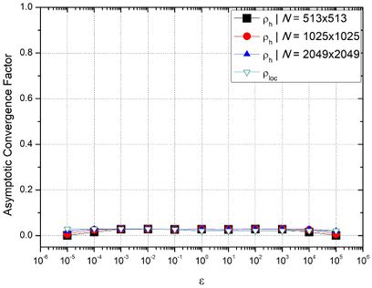
| − | Fig. 7 depicts the numerical asymptotic convergence factor | + | Fig. 7 depicts the numerical asymptotic convergence factor <math>{{\rho }_{loc}}</math> lculated via LFA and the experimental asymptotic convergence factor [[Image:draft_Vassoler Rutz_344011008-image185.png|18px]] , for different anisotropy coefficients for different grids. Algorithm 1 with '''REST''' = <math display="inline">{\mbox{PW}}_\mbox{x}</math> , [[Image:draft_Vassoler Rutz_344011008-image164.png|36px]] and bilinear prolongation was used. As the grid becomes more refined, [[Image:draft_Vassoler Rutz_344011008-image192.png|60px]] for every anisotropy coefficient analyzed, what demonstrates the robustness of the methodology assessed. |
<div class="center" style="width: auto; margin-left: auto; margin-right: auto;"> | <div class="center" style="width: auto; margin-left: auto; margin-right: auto;"> | ||
[[Image:draft_Vassoler Rutz_344011008-image193.jpeg|408px]] </div> | [[Image:draft_Vassoler Rutz_344011008-image193.jpeg|408px]] </div> | ||
| − | Figure 7: | + | Figure 7: <math>{{\rho }_{loc}}</math>and [[Image:draft_Vassoler Rutz_344011008-image189.png|18px]] versus anisotropy coefficients ( [[Image:draft_Vassoler Rutz_344011008-image154.png|12px]] ) for different number of grid points. |
Next section presents the complexity analysis of multigrid. For the analysis, multigrid was built with the components that had the best convergence factors, according to LFA. In addition, a comparison between partial weighting and full weighting will be presented. | Next section presents the complexity analysis of multigrid. For the analysis, multigrid was built with the components that had the best convergence factors, according to LFA. In addition, a comparison between partial weighting and full weighting will be presented. | ||
| Line 773: | Line 768: | ||
| [[Image:draft_Vassoler Rutz_344011008-image158.png|center|42px]] | | [[Image:draft_Vassoler Rutz_344011008-image158.png|center|42px]] | ||
|} | |} | ||
| − | , it can be stated that the lowest values of | + | , it can be stated that the lowest values of <math>{{\rho }_{loc}}</math> are obtained with FW and <math display="inline">{\mbox{PW}}_\mbox{x}</math> restriction operators, and that the values of <math>{{\rho }_{loc}}</math> with these operators are very similar. |
- Using Algorithm 1, [[Image:draft_Vassoler Rutz_344011008-image190.png|90px]] for every anisotropy coefficient assessed and [[Image:draft_Vassoler Rutz_344011008-image192.png|60px]] as the grid becomes more refined. | - Using Algorithm 1, [[Image:draft_Vassoler Rutz_344011008-image190.png|90px]] for every anisotropy coefficient assessed and [[Image:draft_Vassoler Rutz_344011008-image192.png|60px]] as the grid becomes more refined. | ||
Revision as of 03:23, 10 April 2018
Abstract: In this work it is proposed an efficient and robust algorithm for the solution of a physical anisotropy problem. This algorithm is based on the choice of the most efficient restriction operator and on an incomplete LU decomposition suited for each anisotropy direction. Local Fourier analysis is carried out in order to assist the project of an efficient multigrid method. The model considered is pure diffusion with anisotropy aligned to the coordinate axis x. Finite difference method with uniform grid and second-order numerical scheme is used for the discretization of equations. Problems are solved with geometric multigrid method, correction scheme, V-cycle and standard coarsening ratio. The asymptotic convergence factor is calculated for different multigrid components, such as restriction operators, prolongation operators and solvers. Based on the optimum components obtained by LFA, experiments are carried out for the analysis of complexity and computational cost for the algorithm proposed. The main conclusion is that the methodology proposed is efficient for the resolution of problems with strong anisotropy.
Keywords: Physical anisotropy; Multigrid components; Diffusion; Local Fourier analysis.
1. Introduction
Computational Fluid Dynamics (CFD) is a branch of Computational Science that studies numerical methods for the simulation of fluid flows problems. It is known that these methods usually require a high computational cost. In general, this happens because the problems that have to be solved require the resolution of algebraic equation systems whose coefficients matrices are large and sparse [1].
Linear systems are obtained with discretization of the mathematical model, which consists in approximating, through algebraic equations, each term of the mathematical model for each grid node or point. This process leads to an algebraic equation system of the form
| (1) |
where is the coefficient matrix, is the variable of interest and is the independent vector.
In CFD, the methods traditionally employed in this process are: Finite Difference Method (FDM) [2], Finite Volume Method (FVM) [3] and Finite Element Method (FEM) [4].
The algebraic equation system given by Eq. (1) can be solved using direct or iterative methods. In this work, iterative methods were employed due to the aforementioned characteristics of linear systems in CFD (sparse and large coefficients matrices), for which iterative methods are recommended. The multigrid method is one of the most effective methods to accelerate the convergence of iterative methods for the resolution of linear or nonlinear systems, isotropic or anisotropic problems, among others [5-7].
Anisotropic problems are fairly common in Engineering and appear in many phenomena, such as in the case of a material with different heat conduction behaviors for different directions. In this case, the coefficients of the differential equations are distinct among themselves and generate, what is called, physical anisotropy. Anisotropies can also appear from discretization of grids with different spacing in each direction, for instance, boundary layer problems. This is called geometric anisotropy [5,6]. The efficiency of the multigrid method has not yet been fully achieved for problems with strong anisotropy, either physical or geometric [8].
Physical anisotropy problems have been investigated by Rabi and de Lemos [9], who discretized the two-dimensional advection-diffusion equation combining null and constant coefficients. Finite volume method was used in the discretization of the equations. Multigrid method was employed using correction scheme, Gauss-Seidel solver and V- and W-cycles. The authors presented a study of the different speed ranges (null and constant), number of grids, number of smoothing steps at each grid level and different solvers. They concluded that there was a significant reduction in the computational effort when the speed range values were increased.
Wienands and Joppich [10] presented an in-depth study on the Local Fourier Analysis (LFA) and its application on several problems, which included anisotropic problems. The authors calculated the convergence factor of the multigrid method for the anisotropic diffusion equation with different solvers and restriction and prolongation operators.
Johannsen [11] solved an anisotropic diffusion problem using finite volume method for discretizing the equations and 9-point incomplete LU (ILU) decomposition method for solving the linear equations systems. The author employed LFA to demonstrate the superior smoothing properties of ILU.
Oliveira et al. [8] assessed geometric anisotropy for different grids and aspect ratios. They also assessed some components of the multigrid method, such as: solvers, type of restriction, number of levels and number of inner iterations, among several coarsening algorithms. They concluded that Partial Weighting (PW) had a good performance.
Vinogradova and Krukier [12] solved a three-dimensional advection-diffusion problem with intermediate anisotropy using FDM for the discretization of the equations and ILU for the resolution of the linear equation systems. They concluded that the proposed methodology is efficient, but it has the disadvantage of having limitations in the coefficients of the mixed derivatives, which has no physical meaning.
Vassoler-Rutz et al. [11] analyzed the effect of physical anisotropy on multigrid method for two anisotropic diffusion problems. They used FAS scheme, V-cycle, and Modified Strongly Implicit (MSI) and Gauss-Seidel (GS) solvers. They concluded that, for strong anisotropies, the complexity order of the multigrid method is not suitable.
Several works on the implementation of the multigrid method found in the literature demonstrate that the choice of the multigrid components is crucial for the convergence or not of the method. Trottenberg et al. [6] state that these choices are difficult and thus small changes can considerably improve convergence. In this sense, LFA can assist these choices as it allows to predict the performance of the multigrid method, since it provides estimates of the converge rates based on the variation of the multigrid method components.
Pinto et. al. [14] solved the anisotropic diffusion problem using ILU in triangular grids. They used LFA to show the good smoothing properties of the solver and the asymptotic convergence of the multigrid.
Franco et. al. [13] performed LFA in transient problems and obtained the critical value of the parameter that represents the level of space-time anisotropy for the 1D and 2D Fourier equations.
In this work, an efficient and robust method for solving physical anisotropy problems using LFA is proposed. A two-dimensional diffusion mathematical model is considered, in which physical anisotropy appears in the coefficients and it will be denominated diffusion anisotropy. Equations were discretized using FDM with second-order central difference scheme.
The asymptotic convergence factor () of the multigrid method was calculated through assessment of the ILU solver in different directions [7] and several restriction and prolongation operators. The results obtained by means of LFA were used to assess the influence of physical anisotropy on computational cost by means of CPU time and number of operations in each V-cycle and at the restriction step.
The remainder of this work is organized as follows: section 2 presents the mathematical and numerical models. Section 3 discusses considerations regarding the LFA used. Section 4 presents the results of the convergence analysis and complexity analysis. Section 5 presents the conclusion.
2. Mathematical and Numerical Models
For the problem presented below, the calculus domain used is given by , and the discretization of the equations is done using a uniform grid with a number of points given by , where and are the number of points in the directions x and y, respectively, including the boundaries.
2.1. Mathematical Model and Discretization
The diffusion anisotropy problem will be assessed through the two-dimension diffusion equation given by Eq. (2) [5,6]
|
|
(2) |
where T is the temperature, is the second derivative of T as a function of , is the second derivative as a function of and .
The source term S and the analytical solution T are given by
|
(3) |
Eq. (2) was discretized using FDM with CDS, resulting in
| (4) |
where is the system unknown.
Fig. 1(b) depicts the notation of the grid points in Fig. 1(a). The points P (central), W (west), E (east), N (north) and S (south) in Fig. 1(b) correspond to the points in Fig. 1(a), respectively.
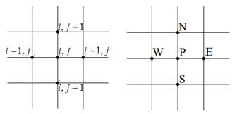 (a) (b) (a) (b)
|
The discretization of Eq. (2) results in Eq. (4), and for the inner points, considering and
,
|
(5) |
For the boundaries north, south, east and west,, .
2.2. Multigrid method and computational details
The multigrid method accelerates the convergence rate of iterative methods. It consists in employing a group of grids with different refinement levels. At each grid refinement level, the more oscillatory errors are smoothed, and only low frequency errors remain. After passing to another grid, the remaining low frequency errors become more oscillatory. The efficiency of this process, called smoothing, depends on the choice of a suitable solver.
For employing multigrid, besides a solver with good smoothing properties, grid transfer operators are required (restriction and prolongation).
In [8] and [16], restriction through partial weighting in the directions and , henceforth denoted by and , respectively, applied in problems involving geometric anisotropy was proposed. These operators, are given in stencil notation as
|
(6) |
In this work, such restriction was combined with 7-point incomplete LU decomposition (henceforth denoted by ILU). According to [17], this decomposition has a better convergence factor than 5-point incomplete LU decomposition for anisotropic problems.
In Eq. (2), discretized using FDM, the stencil for 5-point Laplacian operator is given by
|
|
(7) |
The ILU decomposition of this same operator will be given by
|
|
(8) |
note that in this case, .
Thus, the ILU decomposition is represented by:
|
|
(9) |
where is a lower triangular matrix, is an upper triangular matrix and is the residual matrix.
The iterative process for solving Eq. (4) can be:
|
(10) |
Depending on the ordination of the grid points, different directions can be obtained for the ILU decomposition. In lexicographical order, [17], is given by
|
|
(11) |
Another example of ordination for ILU, [17], is given by
|
(12) |
The linear equation system given by Eq. (1) was solved using the geometric multigrid method [5,6] with correction scheme (CS), V-cycle and zero initial estimate.
The coarsening ratio is given by (standard coarsening) [17]. The grid transfer operators employed were: Injection Restriction (INJ), Half Weighting (HW), Full Weighting (FW) (see [6]), Partial Weighting in ( ), Partial Weighting in () and prolongation by bilinear interpolation and 7-point interpolation. The equation systems obtained by means of discretization were resolved using 7-point ILU solvers in different directions (, , among others).
The stop criterion used to interrupt the iterative process is based on the dimensionless residual norm. The residual of the algebraic equation system is defined by
|
|
(13) |
where is the solution of the unknown in the iteration .
Considering and , if the iterative process is interrupted if .
Double precision arithmetic was used for the simulations. The numerical codes were implemented in the Fortran 2003 language, using the Intel 9.1 Visual Fortran application. All numerical results were obtained in a computer with Intel Core i7 2.66 GHz processor, 16 GB RAM and Windows 8 operating system, 64-bit version.
3. Local Fourier Analysis
LFA allows to predict the performance of the multigrid method as it supplies estimates of the convergence rate of its components. Therefore, LFA becomes a powerful tool in quantitative analysis and for the project of efficient multigrid methods.
In order to perform the LFA, general discrete linear operators with constant coefficients are considered, which are defined in an infinite grid , where the influence of the boundaries can be dismissed [6].
Consider the grid functions of the form of
|
(14) |
where varies in the infinite grid and is a parameter that characterize the frequency of the function concerning to grid .
For , every function of the grid are eigenfunctions of a discrete operator that can be written by a stencil.
Thus,
|
|
(15) |
where
|
(16) |
For the smoothing and the analysis of two grids, it necessary to distinguish components of high and low frequency of in relation to .
It is known that [6] only if
|
(17) |
are visible in .
For each , three other frequency components with coincide in with and are not visible in . Therefore, the low- and high-frequency components are defined as follows:
is a low-frequency component
is a high-frequency component. See Fig. 2.
Figure 2: Low- (inner white area) and high-frequency (hatched area) areas.
Considering the frequencies
|
(18) |
The operator is represented by a 4x4 matrix , as follows
|
(19) |
where is represented by a 4x4 identity matrix, is the 4x4 matrix, is a 1x4 matrix, is a 4x1 matrix and is a 1x1 matrix.
A representation for can be obtained by a matrix of the form
|
(20) |
where is given by Eq. (19) and is a 4x4 matrix and represents .
Let it be
|
(21) |
The asymptotic convergence factor can be calculated by
|
(22) |
where is the spectral radius of the 4x4 matrix .
In this work, LFA was used to determine the asymptotic convergence factor of the multigrid method () combining ILU solvers in several directions (such as and ), FW, HW, INJ, and restriction operators and bilinear and 7-point prolongation operators.
For the FW restriction operator, , for the , and for the , . For the other restriction operators, see [4].
For the bilinear prolongation operator, and for the 7-point prolongation operator, [10].
In order to perform the LFA using the solver, the eigen-functions of , , and are given by
|
(23) |
The smoothing operator , according to [6], is given by
|
(24) |
with
|
|
(25) |
For , and for , .
4. Numerical Results
In this work, the anisotropic diffusion equation was solved using 7-point ILU solver in different directions. Several restriction operators and two prolongation operators were employed. It is proposed an algorithm that presents the lowest asymptotic convergence factor values and the lowest computational cost for the multigrid method.
Eq. (2) was assessed for and , with . When or in this work, there is symmetric anisotropy. For instance, is an anisotropy symmetric to .
Section 4.1 presents the convergence analysis by means of LFA. Only the optimum components obtained via LFA will be used in the complexity analysis in section 4.2.
4.1. Convergence Analysis
Fig. 3 depicts , given by Eq. (22), with in the EN, NE, ES, SE directions, FW restriction, bilinear prolongation, number of inner iterations ,and , with .
Figure 3: versus anisotropy coefficients ( ![]() ) with in different directions.
) with in different directions.
It is noticed that for ![]() , has a good performance and for
, has a good performance and for
| |
has a good performance as well, that is, ![]() . By using solvers in the ES and SE directions, the multigrid did not present a good performance for any of the anisotropy coefficients studied.
. By using solvers in the ES and SE directions, the multigrid did not present a good performance for any of the anisotropy coefficients studied.
For the analyses presented below, tests were carried out using only the solvers that had the best performances in the previous analysis.
Fig. 4 presents using as solvers, for ![]() and for
and for ![]() ;
; ![]() ; FW restriction; 7-point and bilinear prolongation;
; FW restriction; 7-point and bilinear prolongation; ![]() and
and ![]() , with
, with ![]() .
.
Figure 4: versus anisotropy coefficients ( ![]() ) with different interpolation operators.
) with different interpolation operators.
It is observed that the restriction|prolongation combinations FW|bilinear and FW|7-points had a good performance ( ![]() ) and presented very similar convergence factors.
) and presented very similar convergence factors.
Bilinear prolongation operator was used in the following analysis as it is easy to program and demands fewer memory resources. The asymptotic convergence factors were compared with different restriction operators.
Fig. 5 presents using as solvers, for ![]() and for
and for ![]() ;
; ![]() ; FW, HW, INJ, and restriction; bilinear prolongation;
; FW, HW, INJ, and restriction; bilinear prolongation; ![]() and
and ![]() , with
, with ![]() .
.
Figure 5: versus anisotropy coefficients ( ![]() ) with different restriction operators.
) with different restriction operators.
Fig. 5 shows that for ![]() and
and ![]() , with
, with ![]() (symmetric anisotropies),
(symmetric anisotropies), ![]() presents very similar values. It is noted that for anisotropic problems (
presents very similar values. It is noted that for anisotropic problems ( ![]() ), the lowest values for are achieved with FW and restriction, which present very similar values.
), the lowest values for are achieved with FW and restriction, which present very similar values.
Based on the results shown, it is proposed Algorithm 1, which combines ILU solver in different directions with FW and restrictions. The algorithm will be presented now. The abbreviation REST, used in the algorithm, represents any of the restrictions (FW or ) previously defined.
Algorithm1:
___________________________________________________________________________
Apply smoothing with REST restriction
Apply smoothing with FW restriction
else
Apply REST restriction
end if
___________________________________________________________________________
Next, it is presented the asymptotic convergence factor , calculated via LFA, and the empiric asymptotic convergence factor ![]() , for different anisotropy coefficients.
, for different anisotropy coefficients.
Fig. 6 shows Algorithm 1 with REST , ![]() and bilinear prolongation.
and bilinear prolongation.
Figure 6: and ![]() versus anisotropy coefficients (
versus anisotropy coefficients ( ![]() ).
).
It is observed that ![]() for every anisotropy coefficients assessed. Moreover, calculated via LFA is in accordance with
for every anisotropy coefficients assessed. Moreover, calculated via LFA is in accordance with ![]() calculated experimentally.
calculated experimentally.
Fig. 7 depicts the numerical asymptotic convergence factor lculated via LFA and the experimental asymptotic convergence factor ![]() , for different anisotropy coefficients for different grids. Algorithm 1 with REST = ,
, for different anisotropy coefficients for different grids. Algorithm 1 with REST = , ![]() and bilinear prolongation was used. As the grid becomes more refined,
and bilinear prolongation was used. As the grid becomes more refined, ![]() for every anisotropy coefficient analyzed, what demonstrates the robustness of the methodology assessed.
for every anisotropy coefficient analyzed, what demonstrates the robustness of the methodology assessed.
Figure 7: and ![]() versus anisotropy coefficients (
versus anisotropy coefficients ( ![]() ) for different number of grid points.
) for different number of grid points.
Next section presents the complexity analysis of multigrid. For the analysis, multigrid was built with the components that had the best convergence factors, according to LFA. In addition, a comparison between partial weighting and full weighting will be presented.
4.2. Complexity Analysis
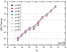
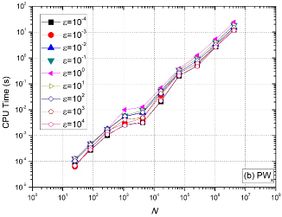
In order to assess the effect of the number of unknowns on CPU time, optimum components obtained via LFA were used. Figures 8 (a) and 8 (b) show, for FW and restrictions respectively, that for the anisotropic problem ( ![]() ), the is not lower. As the problem becomes more anisotropic (
), the is not lower. As the problem becomes more anisotropic ( ![]() or
or ![]() ), the
), the ![]() decreases for every N value assessed. For every anisotropy coefficient assessed, the
decreases for every N value assessed. For every anisotropy coefficient assessed, the ![]() with FW restriction is very similar to the
with FW restriction is very similar to the ![]() with restriction, that is, .
with restriction, that is, .
It is also observed for symmetric anisotropies ( ![]() and
and ![]() ) with
) with ![]() , that the values of
, that the values of ![]() obtained are extremely similar.
obtained are extremely similar.
In order to assess the performance of the multigrid with different anisotropy coefficients, a curve adjustment of the form ![]() [18] was made, where p represents the complexity order of the solver, N is the number of grid points and c is a constant that depends on the method. The closer the value of p is to one, the better the performance of method used. Ideally, multigrid presents p=1, what means that the CPU time grows linearly with the increase of N. Results are shown in Table 1 for both restrictions assessed (FW and ).
[18] was made, where p represents the complexity order of the solver, N is the number of grid points and c is a constant that depends on the method. The closer the value of p is to one, the better the performance of method used. Ideally, multigrid presents p=1, what means that the CPU time grows linearly with the increase of N. Results are shown in Table 1 for both restrictions assessed (FW and ).
One can observe in Tab. 1 that, for every anisotropy employed, the multigrid method has a good performance, since p ≈ 1 in every case. These results prove the efficiency and robustness of Algorithm 1, proposed in this work.
| |
|
|
| |
1.07747 | 1.07733 |
| |
1.05023 | 1.05894 |
| 1 | 1.05940 | 1.04380 |
| |
1.07255 | 1.06199 |
| |
1.07627 | 1.07775 |
The values obtained for the convergence factor, presented in section 4.1, and for the complexity order concerning to the and FW restriction operators (Tab. 1) are quite similar and thus, insufficient to decide which one results in a more efficient algorithm.
To complement the analysis, the number of arithmetical operations performed in each V-cycle and at the restriction step for each one of the operators was assessed.
These arithmetical operations concern to floating point operations (flops) performed during the iterative process and are not affect by the hardware used. Each addition, multiplication and division operation correspond to 1 flop.
Tests were carried out for ![]() (
( ![]() is the number of points of the finest grid, considering a problem whose maximum number of levels is
is the number of points of the finest grid, considering a problem whose maximum number of levels is ![]() ) and for some values of
) and for some values of ![]() . Tab. 2 presents the ratio between number of flops of a V-cycle and number of points of the finest grid
. Tab. 2 presents the ratio between number of flops of a V-cycle and number of points of the finest grid ![]() . Tab. 3 shows the ratio between number of flops performed in each restriction and the number of points of the finest grid
. Tab. 3 shows the ratio between number of flops performed in each restriction and the number of points of the finest grid ![]() .
.
| |
|
|
| |
1510.221554 | 1543.296057 |
| |
1798.299366 | 1837.988770 |
| |
2368.277388 | 2126.896785 |
| |
1860.997604 | 1900.687008 |
| |
1564.958717 | 1598.033220 |
Table 2. Ratio between number of flops of a V-cycle and the number of points of the finest grid.
| |
||
| |
11.57607615 | 44.65057942 |
| |
13.89129130 | 53.58069530 |
| |
18.37833483 | 62.02688007 |
| |
13.89129137 | 53.58069530 |
| |
11.57607615 | 44.65057942 |
Table 3. Ratio between number of flops of the restriction and number of points of the finest grid.
According to Tab. 2, the multigrid cycle that requires the lowest number of flops is the cycle with operator, except for the isotropic case ( ![]() ). Considering only the restriction step, results presented in Tab. 3 show a great advantage of the operator over the FW operator regarding the number of flops performed. For every case, the number of flops for is roughly 75% lower than the number of flops for FW.
). Considering only the restriction step, results presented in Tab. 3 show a great advantage of the operator over the FW operator regarding the number of flops performed. For every case, the number of flops for is roughly 75% lower than the number of flops for FW.
The remaining anisotropy coefficients assessed showed similar performances to those presented in Fig. 5 and Tables 2 and 3, what confirms the efficiency and robustness of the algorithm proposed, in addition to the low computational cost with the use of the operator.
5. Conclusions
- Among the ILU directions assessed (EN, NE, ES, SE) for standard multigrid (FW restriction operator and bilinear prolongation), it is concluded that when using for ![]() and for
and for ![]() .
.
- With FW restriction, for ![]() and
and
, it can be concluded that the 7-point and bilinear prolongation operators presented a similar performance, and for every value of ![]() assessed,
assessed, ![]() was obtained.
was obtained.
- With bilinear interpolation, for ![]() and
and
, it can be stated that the lowest values of are obtained with FW and restriction operators, and that the values of with these operators are very similar.
- Using Algorithm 1, ![]() for every anisotropy coefficient assessed and
for every anisotropy coefficient assessed and ![]() as the grid becomes more refined.
as the grid becomes more refined.
- The for every value of ![]() assessed.
assessed.
- The complexity order p of the multigrid method with Algorithm 1 is close to one for every anisotropy assessed. For ![]() , for example, p=1.07747 with this algorithm.
, for example, p=1.07747 with this algorithm.
- The computational cost of multigrid depends on the number of flops of the restriction in a V-cycle. Using Algorithm 1 with restriction, the computational cost is 75% lower than with FW restriction.
- The Algorithm 1 with restriction proposed in this work is efficient, robust and has low computational cost.
References
- [1] T. Gradl, K. Klamroth, U. Rüde, U. Optimizing the number of multigrid cycles in the full multigrid algorithm. Numerical Linear Algebra with Applications. Vol. 17 (2010) 199–210.
- [2] R. H. Pletcher, J. C. Tannehill, D. A. Anderson, Computational Fluid Mechanics and Heat Transfer, 3ª ed. CRC Press, USA, 2013.
- [3] G. H. Golub, J. M. Ortega, Scientific Computing and Differential Equations: an Introduction to Numerical Methods, Academic Press, 1992.
- [4] Y. Saad, Iterative Methods for Sparse Linear Systems, 2ªed., PWS, Philadelphia, 2003.
- [5] W. L. Briggs, V.E. Henson, S.F. Mccormick, A Multigrid Tutorial, 2ª ed., SIAM, USA, 2000.
- [6] U. Trottenberg, C. Oosterlee, A. Schüller, Multigrid, Academic Press, England, 2001.
- [7] P. Wesseling, An Introduction to Multigrid Methods, John Wiley & Sons, England, 1992.
- [8] F. Oliveira, M. A. V. Pinto, C. H. Marchi, L. K. Araki. Optimized partial semicoarsening multigrid algorithm for heat diffusion problems and anisotropic grids. Applied Mathematical Modelling. Vol. 36 (2012) 4665–4676.
- [9] J. A. Rabi, M. J. S. de Lemos. Optimization of convergence acceleration in multigrid numerical solutions of conductive-convective problems. Applied Mathematics and Computational. Vol. 124 (2001) 215-226.
- [10] R. Wienands, W. Joppich, Practical Fourier Analysis for Multigrid Methods, CRC Press, USA, 2005.
- [11] K. Johannsen. A robust 9-point ILU smoother for anisotropic problems, IWR Preprint, University of Heidelberg, 2005.
- [12] S. A. Vinogradova, L. A. Krukier, The use of incomplete LU decomposition in modeling convection-diffusion processes in an anisotropic medium. Mathematical Models and Computer Simulations. Vol. 5 (2013) 190-197.
- [13] G. Vassoler-Rutz, M. A. V. Pinto, R. Suero, Comparison of the physical anisotropy of multigrid method for two-dimensional diffusion equation, in: Proceedings of COBEM, Rio de Janeiro, Brazil, Dezembro 6-11.
- [14] M. A. V. Pinto, C. Rodrigo, F. J. Gaspar, C.W. Oosterlee. On the robustness of ILU smoothers on triangular grids, Applied Numerical Mathematics. Vol. 106 (2016), 37-52.
- [15] S. R. Franco, F. J. Gaspar, M. A. V. Pinto, C. Rodrigo. Multigrid method based on a space-time approach with standard coarsening for parabolic problems. Applied Mathematics and Computation. Vol. 317 (2018) 25-34.
- [16] F. Oliveira. Effect of Two-Dimensional Anisotropic Meshes on the Performance of the Geometric Multigrid Method. Tese de doutorado, UFPR, 2010. In portuguese.
- [17] P. Wesseling, C. W. Oosterlee. Geometric Multigrid with Applications to Computational Fluid Dynamics. Journal of Computation and Applied Mathematics. Vol. 128 (2001) 311-334.
- [18] R. L. Burden, J.D. Faires, Numerical Analysis, 9ª ed., Cengage Learning, USA, 2010.
Document information
Published on 11/03/19
Accepted on 07/03/19
Submitted on 09/04/18
Volume 35, Issue 1, 2019
DOI: 10.23967/j.rimni.2019.03.001
Licence: CC BY-NC-SA license
