Integration of game theory and response surface method for robust parameter design

Abstract

Robust parameter design (RPD) is to determine the optimal controllable factors that minimize the variation of quality performance caused by noise factors. The dual response surface approach is one of the most commonly applied approaches in RPD that attempts to simultaneously minimize the process bias (i.e., the deviation of the process mean from the target) as well as variance. In order to address this tradeoff issue between the process bias and variance, a number of RPD methods are reported in literature by assigning relative weights or priorities to both the process bias and variance. However, the relative weights or priorities assigned are often subjectively determined by a decision maker (DM) who in some situations may not have enough prior knowledge to determine the relative importance of both the process bias and variance. In order to address this problem, this paper proposes an alternative approach by integrating the bargaining game theory into an RPD model to determine the optimal factor settings. Both the process bias and variance are considered as two rational players that negotiate how the input variable values should be assigned. Then Nash bargaining game solution technique is applied to determine the optimal, fair, and unique solutions (i.e., a balanced agreement point) for this game. This technique may provide a valuable recommendation for the DM to consider before making the final decision. This proposed method may not require any preference information from the DM by considering the interaction between the process bias and variance. To verify the efficiency of the obtained solutions, a lexicographic weighted Tchebycheff method which is often used in bi-objective optimization problems is utilized. Finally, in two numerical examples, the proposed method provides non-dominated tradeoff solutions for a particular convex Pareto frontier case. Furthermore, sensitivity analyses are also conducted for verification purposes associated with the disagreement and agreement points.

Keywords: robust parameter design, lexicographic weighted Tchebycheff, bargaining game, response surface methodology, dual response model

1. Introduction

Due to fierce competition among manufacturing companies and an increase in customer quality requirements, robust parameter design (RPD), an essential method for quality management, is becoming ever more important. RPD was developed to decrease the degree of unexpected deviation from the requirements that are proposed by customers or a DM and thereby helps to improve the quality and reliability of products or manufacturing processes. The central idea of RPD is to build quality into the design process by identifying an optimal set of control factors that make the system impervious to variation [1]. The objectives of RPD are set out to ensure that the process mean is at the desired level and process variance is minimized. However, in reality, a simultaneous realization of those two objectives sometimes is not possible. As Myers et al. [2] stated there are circumstances where the process mean and variance are robust against the effects of noise factors but the mean value is still far away from the target. In other words, a set of parameter values that satisfies these two conflicting objectives may not exist. Hence, the tradeoffs that exist between the process mean and variance are undoubtedly crucial in determining a set of controllable parameters that optimize quality performance.  

The tradeoff issue between the process bias (i.e., the deviation of a process mean from the target value) and variance can be associated with assigning different weights or priority orders. Weight-based methods assign different weights to the process bias and variance, respectively, to establish their relative importance and transform the bi-objective problem into a single objective problem. The two most commonly applied weight-based methods are the mean square error model [3] and the weighted sum model [4,5]. Alternatively, priority-based methods sequentially assign priorities to the objectives (i.e., minimization of the process bias or variance). For instance, if the minimization of the process bias is prioritized, then the process variance is optimized with a constraint of zero-process bias [6]. Other priority-based approaches are discussed by Myers and Carter [7], Copeland and Nelson [8] , Lee et al. [9], and Shin and Cho [10]. In both weight-based and priority-based methods, the relative importance can be assigned by the decision maker’s (DM) preference, which is obviously subjective. Additionally, there are situations in which the DM could be unsure about the relative importance of the process parameters in bi-objective optimization problems.

Therefore, this paper aims to solve this tradeoff problem from a game theory point of view by integrating bargaining game theory into the RPD procedure. First, the process bias and variance are considered as two rational players in the bargaining game. Furthermore, the relationship functions for the process bias and variance are separately estimated by using the response surface methodology (RSM). In addition, those estimated functions are regarded as utility functions that represent players’ preferences and objectives in this bargaining game. Second, a disagreement point, signifying a pair of values that the players expect to receive when negotiation among players break down, can be defined by using the minimax-value theory which is often used as a decision rule in game theory. Third, Nash bargaining solution techniques are then incorporated into the RPD model to obtain the optimal solutions. Then, to verify the efficiency of the obtained solutions, a lexicographic weighted Tchebycheff approach is used to generate the associated Pareto frontier so that it can be visually observed if the obtained solutions are on the Pareto frontier. Two numerical examples are conducted to show that the proposed model can efficiently locate well-balanced solutions. Finally, a series of sensitivity analyses are also conducted in order to demonstrate the effects of the disagreement point value on the final agreed solutions.

This research paper is laid out as follows: Section 2 discusses existing literature for RPD and game theory applications. In Section 3, the dual response optimization problem, the lexicographic weighted Tchebycheff method, and Nash bargaining solution are explained. Next, in Section 4, the proposed model is presented. Then in Section 5, two numerical examples are addressed to show the efficiency of the proposed method, and sensitivity studies are performed to reveal the influence of disagreement point values on the solutions. In Section 6, a conclusion and further research directions are discussed.

2.  Literature review

2.1 Robust parameter design

Taguchi proposed both experimental design concepts and parameter tradeoff issues into a quality design process. In addition, Taguchi developed an orthogonal-array based experimental design and used the signal-to-noise (SN) ratio to measure the effects of factors on desired output responses. As discussed by Leon, Shoemaker, and Kackar [11] in some situations, the SN ratio is not independent of the adjustment parameters, so using the SN ratio as a performance measure may often lead to far from the optimal design parameter settings. Box [12] also argued that statistical analyses based on experimental data should be introduced, rather than relying only on the maximization of the SN ratio. The controversy about the Taguchi method is further discussed and addressed by Nair et al. [13] and Tsui [14].

Based on Taguchi’s philosophy, further statistical based methods for RPD have been developed. Vining and Myers [6] introduced a dual response method, which takes zero-process bias as a constraint and minimizes the variance. Copeland and Nelson [15] proposed an alternative method for the dual response problem by introducing a predetermined upper limit on the deviation from the target. Similar approaches related to upper limit concept are further discussed by Shin and Cho [10] and Lee et al. [9] For the estimation phase, Shoemaker et al. [16] and Khattree [17] suggested a utilization of response surface model approaches. However, when a homoscedasticity assumption for regression is violated, then other methods, such as the generalized linear model, can be applied [18].  Additionally, in cases where there is incomplete data, Lee and Park [19] suggested an expectation-maximization (EM) algorithm to provide an estimation of the process mean and variance, while Cho and Park [20] suggested a weighted least squares (WLS) method. However, Lin and Tu [3] pointed out that the dual response approach had some deficiencies and proposed an alternative method called mean-squared-error (MSE) model. Jayaram and Ibrahim [21] modified the MSE model by incorporating capability indexes and considered the minimization of total deviation of capability indexes to achieve a multiple response robust design. More flexible alternative methods that could obtain Pareto optimal solutions based on a weighted sum model were introduced by many researchers [4,5,22]. In fact, this weighted sum model is more flexible than conventional dual response models, but it cannot be applied when a Pareto frontier is nonconvex [23]. In order to overcome this problem, Shin and Cho [23] proposed an alternative method called lexicographic weighted Tchebycheff by using an L-∞ norm.

More recently, RPD has become more widely used not only in manufacturing but also in other science and engineering areas including pharmaceutical drug development. New approaches such as simulation, multiple optimization techniques, and neural networks (NN) have been integrated into RPD. For example, Le et al. [24] proposed a new RPD model by introducing a NN approach to estimate dual response functions. Additional, Picheral et al. [25] estimated the process bias and variance function by using the propagation of variance method. Two new robust optimization methods, the gradient-assisted and quasi-concave gradient-assisted robust optimization methods, were presented by Mortazavi et al. [26].

2.2 Game Theory

The field of game theory presents mathematical models of strategic interactions among rational agents [51]. These models can become analytical tools to find the optimal choices for interactional and decision-making problems. Game theory is often applied in situations where the "roles and actions of multiple agents affect each other" [27]. Thus, game theory serves as an analysis model that aims at helping agents to make the optimal decisions, where agents are rational and those decisions are interdependent.  Because of the condition of interdependence each agent has to consider other agents’ possible decisions when formulating a strategy. Based on these characteristics of game theory, it is widely applied in multiple disciplines, such as computer science [28], network security and privacy [29], cloud computing [30], cost allocation [31], and construction [32]. Because game theory has a degree of conceptual overlap with optimization and decision-making, three concepts (i.e., game theory, optimization, and decision-making) can often be combined, respectively. According to Sohrabi and Azgom [19], there are three kinds of basic combinations associated with those three concepts as follows: game theory and optimization, game theory and decision-making, game theory, optimization and decision-making.

The first type of these combinations (i.e., game theory and optimization) further has two possible situations. In the first situation, optimization techniques are used to solve a game problem and prove the existence of equilibriums[33,34]. In the second situation, game theory concepts are integrated to solve an optimization problem. For example, Leboucher et al. [35] used evolutionary game theory to improve the performance of a particle swarm optimization (PSO) approach. Additionally, Annamdas and Rao [36] solved a multi-objective optimization problem by using a combination of game theory and a PSO approach. The second type kind of combinations (i.e., game theory and decision-making) integrates game theory to solve a decision-making problem, as discussed by Zamarripa et al. [37] who applied game theory to assist with decision-making problems in supply chain bottlenecks. More recently, Dai et al. [38] attempted to integrate the Stackelberg leadership game into RPD model to solve a dual response tradeoff problem. The third type of combinations (i.e., game theory, optimization and decision-making) integrates game theory and optimization to a decision-making problem. For example, a combination of linear programming and game theory was introduced to solve a decision-making problem [39]. Doudou et al. [40] used a convex optimization method and game theory to settle a wireless sensor network decision-making problem.

2.3 Bargaining game

A bargaining game can be applied in a situation where a set of agents have an incentive to cooperate, but have conflicting interests over how to distribute the payoffs generated from the cooperation [41]. Hence, a bargaining game essentially has two features: Cooperation and conflict. Because the bargaining game considers cooperation and conflicts of interest as a joint problem, it is more complicate than a simple cooperative game that ignores individual interests and maximizes the group benefit [42]. Typical three bargaining game examples include a price negotiation problem between product sellers and buyers, a union and firm negotiation problem over wages and employment levels, and a simple cake distribution problem.

Significant discussions about the bargaining game can be addressed by John Nash [43,43]. Nash [43] presented a classical bargaining game model aimed at solving an economic bargaining problem, and used a numerical example to prove the existence of multiple solutions. In addition, Nash [44] extended his research to a more general form and demonstrated that there are two possible approaches to solve a two-person cooperative bargaining game. The first approach, called the negotiation model, is used to obtain the solution through an analysis of the negotiation process. The second approach, called the axiomatic method, is applied to solve a bargaining problem by specifying axioms or properties that the solution should obtain. For the axiomatic method, Nash concluded four axioms that the agreed solution called Nash bargaining solution should have. Based on Nash’s philosophy, many researchers attempted to modify Nash's model and proposed a number of different solutions based on different axioms. One famous modified model replaces one of Nash’s axioms in order to reach a fairer unique solution which is called the Kalai-Smorodinky’s solution [45]. Later, Rubinstein [46] addressed a bargaining problem by specifying a dynamic model which explains a bargaining procedure.

3. Models and methods

3.1 Bi-objective robust design model

A general bi-objective optimization problem involves simultaneous optimization of two conflicting objectives (e.g.,  $f_{1}(x)$and $f_{2}(x)$) that can be described in mathematical terms as $\min[f_{1}(x),f_{2}(x)]$ . While in RPD, since it can be infeasible to minimize the process bias and variance simultaneously, a simultaneous optimization of these two process parameters, which are separately estimated by applying RSM, is then transforms to a tradeoff problem between the process bias and variance. This tradeoff problem can be formally expressed as a bi-objective optimization problem [23] as:

$min$ ${\textstyle {\left[{\left\{{\hat {\mu }}\left({\boldsymbol {x}}\right)-\tau \right\}}^{2},\,{\hat {\sigma }}^{2}({\boldsymbol {x}})\right]}^{T}}$ $s.t.$ ${\textstyle {\boldsymbol {x}}\in X\,}$

(1)

where ${\textstyle {\boldsymbol {x}}}$, ${\textstyle X}$, ${\textstyle \tau }$, ${\textstyle {\left\{{\hat {\mu }}\left({\boldsymbol {x}}\right)-\tau \right\}}^{2}}$ , and ${\textstyle {\hat {\sigma }}^{2}({\boldsymbol {x}})}$ represent a vector of design factors, the set of feasible solutions under specified constraints, the target process mean value, and the estimated functions for process bias and variance, respectively.

3.2 Lexicographic weighed Tchebycheff method

A bi-objective robust design problem is generally addressed by introducing a set of parameters, determined by a DM, which represents the relative importance of those two objectives. With the introduced parameters, the bi-objective functions can be transformed into a single integrated function, thus the bi-objective optimization problem can be solved by simply optimizing the integrated function. One way to construct this integrated function is by using the weighted sum of the distance between the optimal solution and the estimated function. Different ways of measuring distance can lead to different solutions, and one of the most common methods is ${\textstyle {L}_{p}}$ metric, where $p=1,2,or\,\infty$. When $p=1$, the metric is called the Manhattan metric, whereas ${\textstyle p=\infty }$, it is named the Tchebycheff metric [47]. Utopia point represents an initial point to apply $L-\infty$ metric in weighted Tchebycheff method and can be obtained by minimizing each objective function separately. The weak Pareto optimal solutions can be obtained by introducing different weights:

${\textstyle \mathrm {min} \,{(\sum _{i=1}^{p}{w}_{i}{\left|{f}_{i}\left({\boldsymbol {x}}\right)-{u}_{i}^{\ast }\right|}^{p})}^{\frac {1}{p}}}$

(2)

where ${\textstyle {u}_{i}^{\ast }}$ and ${\textstyle {w}_{i}}$ denote the utopia point values and weights associated with objective functions, respectively. When $p=\infty$, the above function (i.e., Equation 2) will only consider the largest deviation [33]. Although the weighted Tchebycheff method is an efficient approach, its main drawback is that only weak non-dominated solutions can be guaranteed [48], which is obviously not optimal for the DM. So, Steuer and Choo [49] introduced an interactive weighted Tchebycheff method, which can generate every non-dominated point provided that weights are selected appropriately [34]. Shin and Cho [15] introduced the lexicographic weighted Tchebycheff method to the RPD area. This method is proved to be efficient and capable of generating all Pareto optimal solutions when the process bias and variance are treated as a bi-objective problem. The mathematical model is shown below [15]:

$min$ ${\textstyle \mathrm {\,\,\,[\,} \,\xi ,\,\left[{\left\{{\hat {\mu }}\left({\boldsymbol {x}}\right)-t\right\}}^{2}-{u}_{1}^{\ast }\right]+[{\hat {\sigma }}^{2}\left({\boldsymbol {x}}\right)-{u}_{2}^{\ast }]]}$ $s.t.$ $\,\lambda [{\left\{{\hat {\mu }}\left({\boldsymbol {x}}\right)-t\right\}}^{2}-{u}_{1}^{\ast }]\leq \xi$ $\left(1-\lambda \right)[{\hat {\sigma }}\left({\boldsymbol {x}}\right)-{u}_{2}^{\ast }]\leq \xi$ ${\boldsymbol {x}}\in X$

(3)

where $\xi$ and $\lambda$ represent a non-negative variable and the a weight term associated with process bias and variance, respectively. The Lexicographic weighed Tchebycheff method is utilized as a verification method in this paper. 

3.3 Nash bargaining solution

A two-player bargaining game can be represented by a pair ${\textstyle \,(U,d)}$, where ${\textstyle U\subset {R}^{2}}$and ${\textstyle d\subset {R}^{2}}$. ${\textstyle U=({u}_{1}({\boldsymbol {x}}){,u}_{2}({\boldsymbol {x}}))}$ denotes a pair of obtainable payoffs of the two players, where ${\textstyle {u}_{1}({\boldsymbol {x}})}$ and ${\textstyle {\,u}_{2}\left({\boldsymbol {x}}\right)\,}$ represent the utility functions for player 1 and 2, respectively, and ${\textstyle {\boldsymbol {x}}{\boldsymbol {\,=}}{\boldsymbol {(}}{x}_{1},\,{x}_{2})\,}$ denotes a vector of actions taken by players. ${\textstyle d}$ ( ${\textstyle {d=(d}_{1},{d}_{2})}$) , defined as a disagreement point, represents the payoffs that each player will gain from this game when two players fail to reach a satisfactory agreement [39]. In other words the disagreement point values are the payoffs that each player can expect to receive if a negotiation breaks down. Assuming ${\textstyle {u}_{i}({\boldsymbol {x}})>{d}_{i}}$ where ${\textstyle {u}_{i}({\boldsymbol {x}})\in U}$ for ${\textstyle \,i\,=1,2}$, the set ${\textstyle U\cap \left\{\left({u}_{1}({\boldsymbol {x}}),{u}_{2}({\boldsymbol {x}})\right)\in \,{R}^{2}:\,{u}_{1}({\boldsymbol {x}})\geq {d}_{1};\,{u}_{2}({\boldsymbol {x}})\geq {d}_{2}\right\}}$ is non-empty. As suggested by the expression of the Nash bargaining game ${\textstyle (U,d)}$, the Nash bargaining solution is affected by both the reachable utility range (${\textstyle U}$)and disagreement point value (${\textstyle d}$). Since ${\textstyle U}$ cannot be changed, rational players will decide a disagreement point value to optimize their bargaining position. According to Myerson [36], there are three possible ways to determine the value of a disagreement point. One standard way is to calculate the minimax value for each player.

${d}_{1}=\mathrm {min} \,\mathrm {max} \,{u}_{1}({x}_{1},{x}_{2})\,\,and\,\,{d}_{2}=\mathrm {min} \,\mathrm {max} \,{u}_{2}({x}_{1},{x}_{2})$

（4）

To be more specific, Equation 4 states that, given each possible action for player 2, player 1 has a corresponding best response strategy. Then, among all those best response strategies, player 1 chooses the one that returns the minimum payoff which is defined as a disagreement point value. Following this logic, player 1 can guarantee to receive an acceptable payoff. Another possible way of determining the disagreement point value is to derive the disagreement point value as an effective and rational threat to ensure the establishment of an agreement. The last possibility is to set the disagreement point as the focal equilibrium of the game.

Nash proposed four possible axioms that should be possessed by the bargaining game solution [50,51]:

• Pareto optimality

• Independence of equivalent utility representation (IEUR)

• Symmetry

• Independence of irrelevant alternatives (IIA)

The first axiom states that the solution should be Pareto optimal, which means it should not be dominated by any other point. If the notation ${\textstyle f\left(U,d\right)=\left({f}_{1}\left(U,d\right),\,{f}_{2}\left(U,d\right)\right)\,}$ stands for the Nash bargaining solution to the bargaining problem ${\textstyle (U,d)}$, then the solution ${\textstyle {u}^{\ast }=}$$\left({u}_{1}\left({\boldsymbol {x}}^{\mathit {\boldsymbol {\ast }}}\right),{u}_{2}\left({\boldsymbol {x}}^{\boldsymbol {\ast }}\right)\right)$ can be Pareto efficient if and only if there exists no other point ${\textstyle {u}^{'}=}$$\left({u}_{1}\left({\boldsymbol {x}}^{\mathit {\boldsymbol {'}}}\right),\,{u}_{2}\left({\boldsymbol {x}}^{\boldsymbol {'}}\right)\right)\in U$ such that ${\textstyle {u}_{1}\left({\boldsymbol {x}}^{\boldsymbol {'}}\right)>{u}_{1}\left({\boldsymbol {x}}^{\boldsymbol {\ast }}\right);{u}_{2}\left({\boldsymbol {x}}^{\mathit {\boldsymbol {'}}}\right)\geq {u}_{2}\left({\boldsymbol {x}}^{\boldsymbol {\ast }}\right)}$ or ${\textstyle {\,u}_{1}\left({\boldsymbol {x}}^{\boldsymbol {'}}\right)\geq {u}_{1}\left({\boldsymbol {x}}^{\boldsymbol {\ast }}\right);}$ ${\textstyle {u}_{2}\left({\boldsymbol {x}}^{\boldsymbol {'}}\right)>{u}_{2}\left({\boldsymbol {x}}^{\boldsymbol {\ast }}\right)}$ This implies that there is no alternative feasible solution that is better for one player without worsening the payoff for other players.

The second axiom, IEUR also referred to as scale covariance, states that the solution should be independent of positive affine transformations of utilities.In other words, if a new bargaining game ${\textstyle (G,w)}$ exists, where $G=\{{\alpha }_{1}{u}_{1}({\boldsymbol {x}})+{\beta }_{1},{\alpha }_{2}{u}_{2}({\boldsymbol {x}})+{\beta }_{2}\}$ and $w=({\alpha }_{1}{d}_{1}+{\beta }_{1},{\alpha }_{2}{d}_{2}+{\beta }_{2})\,$ and where ${\bigl (}{u}_{1}({\boldsymbol {x}}),{u}_{2}({\boldsymbol {x}}){\bigr )}\in U$and ${\alpha }_{1}>0,{\alpha }_{2}>0$, then the solution for this new bargaining game (i.e., ${\textstyle f(G,w)}$) can be obtained by applying the same transformations, which is demonstrated by Equation 5 and Figure 1:

$\,\,f(G,\,w)=({\alpha }_{1}{f}_{1}(U,d)+{\beta }_{1},\,{\alpha }_{2}{f}_{2}(U,\,d)+{\beta }_{2})\,$

（5）

Figure 1. Explanation of IEUR axiom

The third axiom “symmetry” represents that the solutions should be symmetric when the bargaining positions of the two players are completely symmetric. This axiom can be explained as if there is no information that can be used to distinguish one player from the other, then the solutions should also be indistinguishable between players [42].

As shown in Figure 2, the last axiom states that if ${\textstyle {U}_{1}\subset {U}_{2}}$ and ${\textstyle f({U}_{2},d)}$ is located within the feasible area ${\textstyle {U}_{1}}$, then ${\textstyle f\left({U}_{1,}d\right)=}$$f({U}_{2},d)$ [43].

Figure 2. Explanation of IIA axiom

The solution function introduced by Nash [44] that satisfies all the four axioms as identifies before can be defined as follows:

${\textstyle f\left(U,\,d\right)=Max\prod _{i=1,2}^{}({u}_{i}({\boldsymbol {x}})-{d}_{i})=}$$Max\,({u}_{1}({\boldsymbol {x}})-{d}_{1})({u}_{2}({\boldsymbol {x}})-{d}_{2})$

(6)

where ${\textstyle {u}_{i}({\boldsymbol {x}})>{d}_{i},\,i=1,2}$. Intuitively, this function is trying to find solutions that maximize each player’s difference in payoffs between the cooperative agreement point and the disagreement point. In simpler terms, Nash selects an agreement point ${\textstyle ({u}_{1}\left({\boldsymbol {x}}^{\ast }\right),{u}_{2}({\boldsymbol {x}}^{\ast }))}$ that maximizes the product of utility gains from the disagreement point ${\textstyle \,({d}_{1},{d}_{2})}$.

4. The proposed model

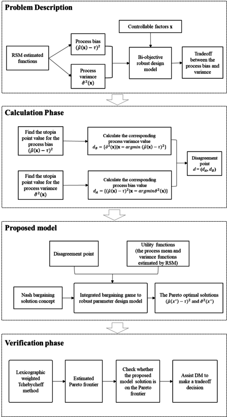
The proposed method attempts to integrate bargaining game concepts into the tradeoff issue between the process bias and variance, so that not only the interaction between process bias and variance can be incorporated but also a unique optimal solution can be obtained. The detailed procedure includes problem description, calculation for response functions and disagreement points, bargaining game based RPD model, and verification can be illustrated in Figure 3. 

An integration of the Nash bargaining game model involves three steps. First step, the two players and their corresponding utility function should be defined. The process bias can be defined as player A, and variance can be regarded as player B. The RSM-based estimated functions of both responses will be regarded as the players’ utility functions in this bargaining game (i.e., ${\textstyle {\,u}_{A}\left({\boldsymbol {x}}\right)\,}$ and ${\textstyle {\,u}_{B}\left({\boldsymbol {x}}\right)}$ ) where ${\boldsymbol {x}}$ stands for a vector of controllable factors. Then, the goal of each player is to choose a set of controllable factors while minimizing each individual utility function. Second step, a disagreement point can be determined by applying a minimax-value theory as identified in Equation 7. Based on the tradeoff between the process bias and variance, the modified disagreement point functions can be defined as follows:

${\textstyle {d}_{A}=\mathrm {max} \,\mathrm {min} \,{u}_{A}({\boldsymbol {x}})\,\,and\,\,{d}_{B}=\mathrm {max} \,\mathrm {min} \,{u}_{B}({\boldsymbol {x}})}$

(7)

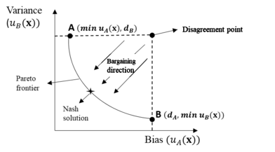
In this way, both player A (i.e., the process bias) and player B (i.e., the process variance) are guaranteed to receive the worst acceptable payoffs.  To be more specific, as demonstrated in Figure 4, if the convex curve represents all Pareto optimal solutions, then each point on the curve can be regarded as a minimum utility value for one of the two process parameters (i.e., the process variance or bias). For example, at point A, when the process bias is minimized within the feasible area, the corresponding variance value is the minimum utility value for the process variance, since other utility values would be either dominated or infeasible. In that case, the disagreement point, defined as the maximum minimum utility value, can be calculated by minimizing only one objective (process variance or bias). The computational functions for the disagreement point values can be formulated as:

${\textstyle \left\{{d}_{A}={u}_{A}({\boldsymbol {x}})|{\boldsymbol {x}}=\arg \min {u}_{B}({\boldsymbol {x}})\,and\,{\boldsymbol {x}}\in X\right\}}$

(8)

and

${\textstyle \left\{{d}_{B}={u}_{B}({\boldsymbol {x}})|{\boldsymbol {x}}=\arg \min {u}_{A}({\boldsymbol {x}})\,and\,{\boldsymbol {x}}\in X\right\}}$

(9)

Figure 3. The proposed procedure by integrating of bargaining game into RPD

Thus, the idea of the proposed method to find the optimal solutions is to continuously perform bargaining games from the specified disagreement point ${\textstyle ({d}_{A},\,{d}_{B})}$ to Pareto frontier as illustrated in Figure 4. These solutions may provide useful insight for a DM when the relative importance between process bias and variance is difficult to identify.  

Figure 4. Solution concepts for the proposed bargaining game based RPD method by integrating trafeoff between both process bias and variance

In the final step, the Nash bargaining solution function ${\textstyle Max\left({u}_{A}({\boldsymbol {x}})-\right.}$$\left.{d}_{A}\right)\left({u}_{B}({\boldsymbol {x}})-{d}_{B}\right)$is utilized. In an RPD problem, the objective of this problem is to minimize both process bias and variance, so a constraint of ${\textstyle {u}_{i}({\boldsymbol {x}})}$< ${\textstyle {d}_{i},\,i=}$$A,B$ is applied. After the players, utility functions and the disagreement point are identified, the Nash bargaining solution function is applied as below:

$max$ ${\textstyle \left({u}_{A}({\boldsymbol {x}})-{d}_{A}\right)\left({u}_{B}({\boldsymbol {x}})-\right.\left.{d}_{B}\right)}$ $s.t.$ ${u}_{A}({\boldsymbol {x}})\leq {d}_{A},{u}_{B}({\boldsymbol {x}})\leq {d}_{B},and\,{\boldsymbol {x}}\in \,X$

(10)

where

$u_{A}({\boldsymbol {x}})={\bigl (}{\widehat {\mu }}({\boldsymbol {x}})-\tau {\bigr )}^{2},\,u_{B}({\boldsymbol {x}})={\hat {\sigma }}^{2}({\boldsymbol {x}})\,or\,{\hat {\sigma }}({\boldsymbol {x}})$

${\hat {\mu }}({\boldsymbol {x}})=\alpha _{0}+{\boldsymbol {x}}^{T}{\boldsymbol {\alpha _{1}}}+{\boldsymbol {x}}^{T}{\boldsymbol {\Gamma }}{\boldsymbol {x}},\,and\,{\hat {\sigma }}^{2}({\boldsymbol {x}})=\beta _{0}+{\boldsymbol {x}}^{T}{\boldsymbol {\beta _{1}}}+{\boldsymbol {x}}^{T}\Delta {\boldsymbol {x}}$

${\hat {\sigma }}({\boldsymbol {x}})=\gamma _{0}+{\boldsymbol {x}}^{T}{\boldsymbol {\gamma _{1}}}+{\boldsymbol {x}}^{T}\mathrm {E} {\boldsymbol {x}}$

and where

${\textstyle {\boldsymbol {x}}=\left[\,{\begin{matrix}{x}_{1}\\{x}_{2}\\\,{\begin{matrix}\vdots \\{x}_{n-1}\\{x}_{n}\end{matrix}}\end{matrix}}\right],\,{\mathit {\boldsymbol {\alpha }}}_{\mathit {\boldsymbol {1}}}=\left[\,{\begin{matrix}{\hat {\alpha }}_{1}\\{\hat {\alpha }}_{2}\\\,{\begin{matrix}\vdots \\{\hat {\alpha }}_{n-1}\\{\hat {\alpha }}_{n}\end{matrix}}\end{matrix}}\right],\,{\mathit {\boldsymbol {\beta }}}_{\mathit {\boldsymbol {1}}}=\,\left[{\begin{matrix}{\hat {\beta }}_{1}\\{\begin{matrix}{\hat {\beta }}_{2}\\\vdots \end{matrix}}\\{\begin{matrix}{\hat {\beta }}_{n-1}\\{\hat {\beta }}_{n}\end{matrix}}\end{matrix}}\right],and\,{\boldsymbol {\Gamma }}=\,\left[{\begin{matrix}{\begin{matrix}{\hat {\alpha }}_{11}&{\hat {\alpha }}_{12}/2\\{\hat {\alpha }}_{12}/2&{\hat {\alpha }}_{22}\end{matrix}}&\cdots &{\begin{matrix}{\hat {\alpha }}_{1n}/2\\{\hat {\alpha }}_{2n}/2\end{matrix}}\\\vdots &\ddots &\vdots \\{\begin{matrix}{\hat {\alpha }}_{1n}/2&{\hat {\alpha }}_{2n}/2\end{matrix}}&\cdots &{\hat {\alpha }}_{nn}\end{matrix}}\right]}$

${\boldsymbol {\Delta }}=\,\left[{\begin{matrix}{\begin{matrix}{\hat {\beta }}_{11}&{\hat {\beta }}_{12}/2\\{\hat {\beta }}_{12}/2&{\hat {\beta }}_{22}\end{matrix}}&\cdots &{\begin{matrix}{\hat {\beta }}_{1n}/2\\{\hat {\beta }}_{2n}/2\end{matrix}}\\\vdots &\ddots &\vdots \\{\begin{matrix}{\hat {\beta }}_{1n}/2&{\hat {\beta }}_{2n}/2\end{matrix}}&\cdots &{\hat {\beta }}_{nn}\end{matrix}}\right],\,and\,{\boldsymbol {\mathrm {E} }}=\,\left[{\begin{matrix}{\begin{matrix}{\hat {\gamma }}_{11}&{\hat {\gamma }}_{12}/2\\{\hat {\gamma }}_{12}/2&{\hat {\gamma }}_{22}\end{matrix}}&\cdots &{\begin{matrix}{\hat {\gamma }}_{1n}/2\\{\hat {\gamma }}_{2n}/2\end{matrix}}\\\vdots &\ddots &\vdots \\{\begin{matrix}{\hat {\gamma }}_{1n}/2&{\hat {\gamma }}_{2n}/2\end{matrix}}&\cdots &{\hat {\gamma }}_{nn}\end{matrix}}\right]$

where $(d_{A},d_{B})$, $u_{A}({\boldsymbol {x}})$, $u_{B}({\boldsymbol {x}})$, ${\hat {\mu }}({\boldsymbol {x}})$, ${\hat {\sigma }}^{2}({\boldsymbol {x}})$, ${\hat {\sigma }}({\boldsymbol {x}})$, $\tau$, $X$ and x represent a disagreement point, utility functions for player A and B, an estimated process mean function, process variance function, and standard deviation function, the target value, the feasible area, the vector of controllable factors, respectively. In Equation (10), ${\boldsymbol {\alpha _{1}}}$, ${\boldsymbol {\beta _{1}}}$, ${\boldsymbol {\gamma _{1}}}$, ${\boldsymbol {\Gamma }}$, ${\boldsymbol {\Delta }}$, and ${\boldsymbol {\mathrm {E} }}$ denote vectors and matrixes of estimated regression coefficients for the process mean, variance, standard deviation, respectively. Here, the constraint, $u_{i}({\boldsymbol {x}})\leq d_{i}$where $i=A,B$, ensures that the obtained agreement point payoffs will be at least as good as the disagreement point payoffs. Otherwise, there is no reason for players to participate in the negotiation.

5. Numerical illustrations and sensitivity analysis

5.1 Numerical example 1

Two numerical examples are conducted to demonstrate the efficiency of the proposed method. Example 1 investigates the relationship between the coating thickness of bare silicon wafers ($y$) and three controller variables: mould temperature ${\textstyle ({x}_{1})}$, injection flow rate ${\textstyle ({x}_{2})}$, and cooling rate ${\textstyle {(x}_{3})}$ [10]. A central composite design and three replications were conducted, and the detailed experimental data with coded values can be shown in Table 1.

Table 1. Data for numerical example 1

Experiments number	$x_{1}$	$x_{2}$	$x_{3}$	$y_{1}$	$y_{2}$	$y_{3}$	$y_{4}$	${\overline {\mathit {y}}}$	${\mathit {\sigma }}$
1	-1	-1	-1	76.30	80.50	77.70	81.10	78.90	2.28
2	1	-1	-1	79.10	81.20	78.80	79.60	79.68	1.07
3	-1	1	-1	82.50	81.50	79.50	80.90	81.10	1.25
4	1	1	-1	72.30	74.30	75.70	72.70	73.75	1.56
5	-1	-1	1	70.60	72.70	69.90	71.50	71.18	1.21
6	1	-1	1	74.10	77.90	76.20	77.10	76.33	1.64
7	-1	1	1	78.50	80.00	76.20	75.30	77.50	2.14
8	1	1	1	84.90	83.10	83.90	83.50	83.85	0.77
9	-1.682	0	0	74.10	71.80	72.50	71.90	72.58	1.06
10	1.682	0	0	76.40	78.70	79.20	79.30	78.40	1.36
11	0	-1.682	0	79.20	80.70	81.00	82.30	80.80	1.27
12	0	1.682	0	77.90	76.40	76.90	77.40	77.15	0.65
13	0	0	-1.682	82.40	82.70	82.60	83.10	82.70	0.29
14	0	0	1.682	79.70	82.40	81.00	81.20	81.08	1.11
15	0	0	0	70.40	70.60	70.80	71.10	70.73	0.30
16	0	0	0	70.90	69.70	69.00	69.90	69.88	0.78
17	0	0	0	70.70	71.90	71.70	71.20	71.38	0.54
18	0	0	0	70.20	71.00	71.50	70.40	70.78	0.59
19	0	0	0	71.50	71.10	71.20	70.00	70.95	0.66
20	0	0	0	71.00	70.40	70.90	69.90	70.55	0.51

The fitted response functions for the process bias and standard deviation of the coating thickness are estimated by using a MINITAB software package as:

${\hat {\mu }}\left({\boldsymbol {x}}\right)=\,72.21+\,{\boldsymbol {x}}^{T}{\boldsymbol {\alpha }}_{\boldsymbol {1}}{\mathit {\boldsymbol {+\,}}}{\boldsymbol {x}}^{T}{\boldsymbol {A\,x}}$

(11)

where ${\boldsymbol {\mathrm {a} }}=\,\left[{\begin{matrix}0.59\\-0.35\\-0.01\end{matrix}}\right]\quad$and $\quad {\boldsymbol {\mathrm {A} }}=\,\left[{\begin{matrix}0.28&0.045&0.83\\0.045&1.29&0.755\\0.83&0.755&1.85\end{matrix}}\right]$

${\textstyle {\hat {\sigma }}\left({\boldsymbol {x}}\right)=\,2.55\,+{{\boldsymbol {x}}^{\mathit {\boldsymbol {T}}}{\mathit {\boldsymbol {\beta }}}}_{\mathit {\boldsymbol {1}}}{\mathit {\boldsymbol {+\,}}}{\boldsymbol {x}}^{\mathit {\boldsymbol {T}}}{\boldsymbol {Bx}}}$

(12)

where ${\boldsymbol {\mathrm {b} }}=\,\left[{\begin{matrix}0.38\\-0.43\\0.56\end{matrix}}\right]\quad$ and $\quad {\boldsymbol {\mathrm {B} }}=\,\left[{\begin{matrix}0.49&-0.235&0.36\\-0.235&0.61&-0.06\\0.36&-0.06&0.85\end{matrix}}\right]$

Based on the proposed RPD procedure as described in Figure 3, those two functions (i.e., process bias and standard deviation) as shown in Equation (11) and (12) are regarded as two players and also their associated utility functions in the bargaining game.  The disagreement point as shown in Figure 4 can be computed as ${\textstyle d=({d}_{\mathit {\boldsymbol {A}}}}$, ${\textstyle {d}_{\mathit {\boldsymbol {B\,}}})}$=(1.2398, 3.1504)  by using Equations (8) and (9).Then, the optimization problem can be solved by applying Equation (10) under an additional constraint, ${\textstyle \sum _{l=1}^{3}{{x}_{l}}^{2}\leq 3}$. which represents a feasible experiment region.

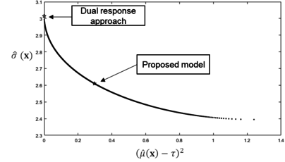
The solution (i.e., ${\textstyle {\left({\hat {\mu }}\left({\boldsymbol {x}}\right)-\tau \right)}^{2}=}$ 0.2967 and ${\textstyle {\hat {\sigma }}\left({\boldsymbol {x}}\right)}$ = 2.6101) are calculated by using a MATLAB software package. To perform a comparative study, the optimization results of the proposed method and the conventional dual response approach are summarized in Table 2. Based on Table 2, the proposed method provides slightly better MSE results in this particular numerical example. To check the efficiency of the obtained results, the lexicographic weighted Tchebycheff approach is adopted to procure an associated Pareto frontier which is shown in Figure 5.

Table 2. The optimization results of example1

	${x}_{1}^{\ast }$	${x}_{2}^{\ast }$	${x}_{3}^{\ast }$	${\left({\hat {\mu }}\left({\boldsymbol {x}}^{*}\right)-\tau \right)}^{2}$	${\hat {\sigma }}^{2}{\mathit {\boldsymbol {(}}}{\boldsymbol {x}}^{*}{\mathit {\boldsymbol {)}}}$	MSE
Dual response model with WLS	0.998	0.998	0.998	7.93	45.66	108.48
Proposed model	1.000	0.4440	0.4440	4.8606	58.3974	82.023

Figure 5. The optimization results plot with the Pareto frontier of example 1

As exhibited in Figure 5, the obtained Nash bargaining solution, which is plotted as a star, is on the Pareto frontier. By using the concept of bargaining game theory, the interaction between process bias and variance can be incorporated while identifying a unique tradeoff result. As results, this proposed method might provide well-balanced optimal solutions associated with the process bias and variance in this particular example.

5.2 Sensitivity analysis for numerical example 1

Based on the optimization results, sensitivity analysis for different disagreement point values are then conducted for verification purposes as shown in Table 3. While changing $d_{B}$ values by both 10% increment and decrement with fixed $d_{A}$ value at 3.1504, the changing patterns of the process bias and variance values are investigated in this sensitivity analysis.

Table 3. Sensitivity analysis results for numerical example 1 by changing ${\textstyle {d}_{A}}$

${d}_{A}$	${d}_{B}$	${{\mathit {\boldsymbol {((}}}{\hat {\mu }}\left({\boldsymbol {x}}\right){\mathit {\boldsymbol {-}}}t{\mathit {\boldsymbol {)}}}}^{\mathit {\boldsymbol {2}}}-$${d}_{A}{\boldsymbol {)\ast (}}{\hat {\sigma }}\left({\boldsymbol {x}}\right)-$${d}_{B}{\mathit {\boldsymbol {)}}}$	x	${{\boldsymbol {(}}\mu \left({\boldsymbol {x}}\right){\boldsymbol {-}}\tau {\boldsymbol {)}}}^{\boldsymbol {2}}$	$\sigma \left({\boldsymbol {x}}\right)$
0.6589	3.1504	0.2218	[-1.0281 -0.0159 0.3253]	0.157	2.7085
0.7321	3.1504	0.2547	[-1.0017 -0.0078 0.3107]	0.1753	2.6930
0.8134	3.1504	0.2925	[-0.9739 0.0007 0.2953]	0.1953	2.6771
0.9038	3.1504	0.3361	[-0.9445 0.0098 0.2790]	0.2174	2.6608
1.0042	3.1504	0.3861	[-0.9137 0.0193 0.2619]	0.2416	2.6441
1.1158	3.1504	0.4435	[-0.8813 0.0293 0.2438]	0.2680	2.6272
1.2398	3.1504	0.5095	[-0.8473 0.0399 0.2248]	0.2967	2.6101
1.3638	3.1504	0.5775	[-0.8153 0.0499 0.2069]	0.3248	2.5946
1.5002	3.1504	0.6543	[-0.7820 0.0603 0.1881]	0.3549	2.5791
1.6502	3.1504	0.7412	[-0.7475 0.0711 0.1687]	0.3869	2.5637
1.8152	3.1504	0.8393	[-0.7120 0.0824 0.1486]	0.4209	2.5484
1.9967	3.1504	0.9499	[-0.6754 0.0939 0.1278]	0.4567	2.5335
2.1964	3.1504	1.0746	[-0.6381 0.1058 0.1065]	0.4942	2.5191
2.4160	3.1504	1.2148	[-0.6002 0.1180 0.0847]	0.5331	2.5052

As shown in Table 3, if only ${\textstyle {d}_{A}}$ increases, the optimal squared bias ${\textstyle {({\hat {\mu }}({\boldsymbol {x}})-\tau )}^{2}}$ increases while the process standard deviation ${\textstyle {\hat {\sigma }}\left({\boldsymbol {x}}\right)}$ decreasing. All of the optimal solutions obtained by using the proposed methods are plotted as circles and compared with the Pareto optimal solutions generated by using the lexicographic weighted Tchebycheff method. Clearly, the obtained solutions are on the Pareto frontier, as shown in Figure 6.

Figure 6.  Plot of sensitivity analysis results with the Pareto frontier for numerical example 1 by changing ${\textstyle {d}_{A}}$.

5.2 Numerical example 2

The second example is from Cho and Park [47]; it is an unbalanced data case that studies the relationship between coating thickness ($y$), mould temperature (${\textstyle {x}_{1}}$), and injection flow rate (${\textstyle {x}_{2}}$). The authors used a ${\textstyle {3}^{2}}$ factorial design with three levels, -1, 0, and +1, respectively. The detailed data is shown in Table 2:

TABLE 2. Data for numerical example 2

Experiments number	${\mathit {\boldsymbol {x}}}_{\boldsymbol {1}}$	${\mathit {\boldsymbol {x}}}_{\boldsymbol {2}}$	${\mathit {\boldsymbol {y}}}_{\boldsymbol {1}}$	${\mathit {\boldsymbol {y}}}_{\boldsymbol {2}}$	${\mathit {\boldsymbol {y}}}_{\boldsymbol {3}}$	${\mathit {\boldsymbol {y}}}_{\boldsymbol {4}}$	${\mathit {\boldsymbol {y}}}_{\boldsymbol {5}}$	${\mathit {\boldsymbol {y}}}_{\boldsymbol {6}}$	${\mathit {\boldsymbol {y}}}_{\boldsymbol {7}}$	${\overline {\mathit {\boldsymbol {y}}}}$	${\mathit {\boldsymbol {\sigma }}}^{\mathit {\boldsymbol {2}}}$
1	-1	-1	84.3	57.0	56.5					65.93	253.06
2	0	-1	75.7	87.1	71.8	43.8	51.6			66.00	318.28
3	1	-1	65.9	47.9	63.3					59.03	94.65
4	-1	0	51.0	60.1	69.7	84.8	74.7			68.06	170.35
5	0	0	53.1	36.2	61.8	68.6	63.4	48.6	42.5	53.46	139.89
6	1	0	46.5	65.9	51.8	48.4	64.4			55.40	83.11
7	-1	1	65.7	79.8	79.1					74.87	63.14
8	0	1	54.4	63.8	56.2	48.0	64.5			57.38	47.54
9	1	1	50.7	68.3	62.9					60.63	81.29

Cho and Park (2005) used the weighted least square (WLS) method to estimate the mean and variance function, as:

${\textstyle {\hat {\mu }}\left({\boldsymbol {x}}\right)=\,55.08\,{\mathit {\boldsymbol {+\,}}}{\boldsymbol {x}}^{T}{\boldsymbol {\alpha }}_{\boldsymbol {1}}{\mathit {\boldsymbol {+\,}}}{\boldsymbol {x}}^{T}{\boldsymbol {A\,x}}}$

(17)

where ${\boldsymbol {\mathrm {a} }}=\,\left[{\begin{matrix}-5.76\\-0.52\\\end{matrix}}\right]\quad$and $\quad {\boldsymbol {\mathrm {A} }}=\,\left[{\begin{matrix}5.51&-1.84\\-1.84&5.47\\\end{matrix}}\right]$

${\textstyle {\hat {\sigma }}^{2}\left({\boldsymbol {x}}\right)=\,154.26\,+{{\boldsymbol {x}}^{\mathit {\boldsymbol {T}}}{\mathit {\boldsymbol {\beta }}}}_{\mathit {\boldsymbol {1}}}{\mathit {\boldsymbol {+\,}}}{\boldsymbol {x}}^{\mathit {\boldsymbol {T}}}{\boldsymbol {Bx}}}$

(18)

where ${\boldsymbol {\mathrm {a} }}=\,\left[{\begin{matrix}-39.34\\-93.09\\\end{matrix}}\right]\quad$and $\quad {\boldsymbol {\mathrm {A} }}=\,\left[{\begin{matrix}-38.31&44.14\\44.14&17.81\\\end{matrix}}\right]$

Modifying the mean function as squared bias:

${\textstyle {({\hat {\mu }}({\boldsymbol {x}})-\tau )}^{2}={((55.08-5.76{x}_{1}-0.52{x}_{2}+5.51{x}_{1}^{2}+5.47{x}_{2}^{2}-1.84{x}_{1}{x}_{2})-50)}^{2}}$

(19)

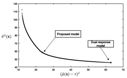
Applying the same logic as in example 1, the process bias is player A and variance as player B. First, the ranges for bias and variance are calculated using the built-in optimization tool called fmincon; these are [12.0508, 420.25] and [45.53, 310.39], respectively. Second, the disagreement points are computed as ${\textstyle {d}_{A}}$ =63.0436 and ${\textstyle {d}_{B}}$=112.0959. Applying function (12) while taking function (13) and ${\textstyle -}$$1<{x}_{k}<1,\,k=1,\,2$ as constraints gives the ultimate answer, ${\textstyle {({\hat {\mu }}({\boldsymbol {x}})-\tau )}^{2}}$=23.6526, ${\textstyle {\hat {\sigma }}^{2}\left({\boldsymbol {x}}\right)=}$ 58.3974. When this result is compared with that of Cho and Park [46] which used a dual response model with WLS estimation method, our result outperforms theirs in terms of MSE (Table 3).

TABLE 3. Optimal solution comparison

	${x}_{1}^{\ast }$	${x}_{2}^{\ast }$	$\left|{\hat {\mu }}{\mathit {\boldsymbol {(}}}{\boldsymbol {x}}{\mathit {\boldsymbol {)-}}}\tau \right|$	${\hat {\sigma }}^{2}{\mathit {\boldsymbol {(}}}{\boldsymbol {x}}{\mathit {\boldsymbol {)}}}$	MSE
Dual response model with WLS	0.998	0.998	7.93	45.66	108.48
Proposed model	1.000	0.4440	4.8606	58.3974	82.023

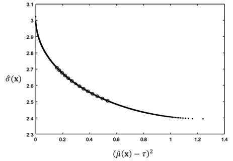
By applying the lexicographic weighted Tchebycheff approach, we can obtain all non-dominated points that form the Pareto optimal frontier (Figure 6). Again, the Nash bargaining solution is on the Pareto frontier, which may provide a valuable suggestion for the trade-off problem.

 Figure 6. Pareto frontier for example 2 and solution plot of the proposed method

5.3 Sensitivity analysis for numerical example 1

In this section, the effect of different disagreement point values will be investigated. In example 1, the disagreement point is${\textstyle d=({d}_{A},{d}_{B{\mathit {\boldsymbol {\,}}}})=}$(1.2398, 3.1504). Now, while the value of ${\textstyle {d}_{B{\mathit {\boldsymbol {\,}}}}}$ is fixed at 3.1504, the value of ${\textstyle {d}_{A{\mathit {\boldsymbol {\,}}}}}$ is changed in steps of 10% (both increase and decrease) and the resulting changes in process bias and variance are investigated.

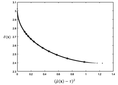
On the contrary, if ${\textstyle {d}_{A}}$ is treated as a constant and ${\textstyle {d}_{B}}$ is changed by 5% each time, the data is transformed as summarized in Table 5 and Figure 8.

Table 5. Example 1 sensitivity analysis; ${\textstyle {d}_{B}}$ is increased and decreased by 5%

${d}_{A}$	${d}_{B}$	${{\mathit {\boldsymbol {((}}}{\hat {\mu }}\left({\boldsymbol {x}}\right){\mathit {\boldsymbol {-}}}t{\mathit {\boldsymbol {)}}}}^{\mathit {\boldsymbol {2}}}-$${d}_{A}{\boldsymbol {)\ast (}}{\hat {\sigma }}\left({\boldsymbol {x}}\right)-$${d}_{B}{\mathit {\boldsymbol {)}}}$	x	${{\boldsymbol {(}}{\hat {\mu }}\left({\boldsymbol {x}}\right){\boldsymbol {-}}\tau {\boldsymbol {)}}}^{\boldsymbol {2}}$	${\hat {\sigma }}\left({\boldsymbol {x}}\right)$
1.2398	2.4377	0.0076	[-0.2082 0.2495 -0.1539]	0.9764	2.4089
1.2398	2.5660	0.0592	[-0.4198 0.1770 -0.0212]	0.7286	2.4501
1.2398	2.7011	0.1394	[-0.5607 0.1307 0.0618]	0.5746	2.4916
1.2398	2.4832	0.2425	[-0.6726 0.0948 0.1262]	0.4595	2.5324
1.2398	2.9929	0.3664	[-0.7666 0.0651 0.1795]	0.3690	2.5721
1.2398	3.1504	0.5095	[-0.8473 0.0399 0.2248]	0.2967	2.6101
1.2398	3.3079	0.6626	[-0.9141 0.0192 0.2621]	0.2412	2.6444
1.2398	3.4733	0.8316	[-0.9727 0.0011 0.2946]	0.1962	2.6764
1.2398	3.6470	1.0162	[-1.0241 -0.0147 0.3231]	0.1597	2.7061
1.2398	3.8293	1.2159	[-1.0692 -0.0285 0.3480]	0.1303	2.7334
1.2398	4.0208	1.4308	[-1.1088 -0.0406 0.3698]	0.1065	2.7583

Figure 8. A plot of all calculated solution points for numerical example 1 when ${\textstyle {d}_{B}}$is changed by 5%

As demonstrated by Table 5, solution value of ${\textstyle {({\hat {\mu }}({\boldsymbol {x}})-\tau )}^{2}}$ declines while ${\textstyle \,{\hat {\sigma }}\left({\boldsymbol {x}}\right)}$ grows if ${\textstyle {d}_{B}}$ is increased and ${\textstyle {d}_{A}}$ is kept constant. However, all of the solution points are still on the Pareto frontier, as shown in Figure 8.

5.4 Sensitivity analysis for numerical example 2

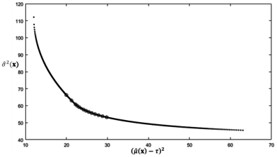
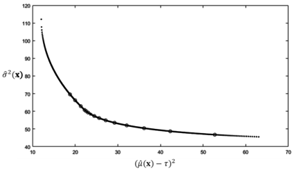
Applying the same logic for example 2, ${\textstyle {d}_{B}}$ is kept constant as ${\textstyle {d}_{A}}$ is changed by 10%. Table 6 exhibits the effect of changes in ${\textstyle {d}_{A}}$, and Figure 9 demonstrates the efficiency of the calculated solutions.

Table 6. Example 2 sensitivity analysis; ${\textstyle {d}_{A}}$ is increased and decreased by 10%

${d}_{A}$	${d}_{B}$	${{\mathit {\boldsymbol {((}}}{\hat {\mu }}\left({\boldsymbol {x}}\right){\mathit {\boldsymbol {-}}}\tau {\mathit {\boldsymbol {)}}}}^{\mathit {\boldsymbol {2}}}-$${d}_{A}{\boldsymbol {)\ast (}}{\hat {\sigma }}^{2}\left({\boldsymbol {x}}\right)-$${d}_{B}{\mathit {\boldsymbol {)}}}$	x	${{\boldsymbol {(}}{\hat {\mu }}\left({\boldsymbol {x}}\right){\boldsymbol {-}}\tau {\boldsymbol {)}}}^{\boldsymbol {2}}$	${\hat {\sigma }}^{\mathit {\boldsymbol {2}}}\left({\boldsymbol {x}}\right)$
37.2266	112.0959	790.0487	[ 0.9510 0.3554]	19.9778	66.2928
41.3629	112.0959	986.2591	[0.9813 0.3624]	21.2437	63.0751
45.9588	112.0959	1218.3	[1.0000 0.3751]	22.2248	60.7647
51.0653	112.0959	1482.5	[1.0000 0.3978]	22.6267	59.9662
56.7392	112.0959	1780.6	[1.000 0.4208]	23.0925	59.1766
63.0436	1120959	2116.7	[1.0000 0.4440]	23.6256	58.3974
69.3480	112.0959	2457.5	[1.0000 0.4653]	24.1686	57.7026
76.2828	112.0959	2837.1	[1.0000 0.4867]	24.7721	57.0185
83.9110	112.0959	3259.8	[1.0000 0.5083]	25.4386	56.346
92.3021	112.0959	3730.5	[1.0000 0.5300]	26.1709	55.686
101.5323	112.0959	4254.2	[1.0000 0.5518]	26.9716	55.0393
111.6856	112.0959	4836.8	[1.0000 0.5738]	27.8435	54.407
122.8541	112.0959	5484.6	[1.0000 0.5958]	28.7892	53.7896
135.1396	112.0959	6204.7	[1.0000 0.6179]	29.8115	53.1879

Figure 9. A plot of all calculated solution points for numerical example 2 when ${\textstyle {d}_{A}}$ is changed by 10%

Likewise, ${\textstyle {d}_{A}}$ is kept constant while ${\textstyle {d}_{B}}$ is changed by 10%. The altered data are summarized in Table 7 and plotted in Figure 10.

Table 7. Example 2 sensitivity analysis; ${\textstyle {d}_{B}}$ is increased and decreased by 10%

${d}_{A}$	${d}_{B}$	${{\mathit {\boldsymbol {((}}}{\hat {\mu }}\left({\boldsymbol {x}}\right){\mathit {\boldsymbol {-}}}\tau {\mathit {\boldsymbol {)}}}}^{\mathit {\boldsymbol {2}}}-$${d}_{A}{\boldsymbol {)\ast (}}{\hat {\sigma }}^{\mathit {\boldsymbol {2}}}\left({\boldsymbol {x}}\right)-$${d}_{B}{\mathit {\boldsymbol {)}}}$	x	${{\boldsymbol {(}}{\hat {\mu }}\left({\boldsymbol {x}}\right){\boldsymbol {-}}\tau {\boldsymbol {)}}}^{\boldsymbol {2}}$	${\hat {\sigma }}^{\mathit {\boldsymbol {2}}}\left({\boldsymbol {x}}\right)$
63.0436	48.2536	15.4253	[1.0000 0.9166]	52.7429	46.7561
63.0436	53.6151	102.0493	[1.0000 0.8094]	42.2936	48.6971
63.0436	59.5724	245.6339	[1.0000 0.7284]	36.1567	50.4366
63.0436	66.1915	438.1362	[1.0000 0.6620]	32.0892	52.0372
63.0436	73.5461	677.0693	[1.0000 0.6055]	29.2313	53.5218
63.0436	81.7179	962.4337	[1.0000 0.5567]	27.1579	54.8985
63.0436	90.7977	1295.7	[1.0000 0.5140]	25.6262	56.1698
63.0436	100.8863	1679.3	[1.0000 0.4767]	24.4832	57.3359
63.0436	112.0959	2116.7	[1.0000 0.4440]	23.6256	58.3974
63.0436	123.3066	2562.1	[1.0000 0.4181]	23.0342	59.2691
63.0436	135.6372	3058.4	[1.0000 0.3951]	22.5764	60.0593
63.0436	149.2010	3609.9	[1.0000 0.3748]	22.2214	60.7721
63.0436	164.1211	4223.7	[0.9829 0.3628]	21.3147	62.9025
63.0436	180.5332	4919.9	[0.9512 0.3554]	19.9864	66.2698
63.0436	198.5865	5708.3	[0.9199 0.3472]	18.7938	69.5842

Figure 10. A plot of all calculated solution points for numerical example 2 when ${\textstyle {d}_{B}}$ is changed by 10%

In conclusion, in both cases, an increase in the value of ${\textstyle {d}_{i}}$ will increase the corresponding bargaining solution value. In other words, an increase in ${\textstyle {d}_{A}}$ will increase the process bias result, and an increase in ${\textstyle {d}_{B}}$ will raise the variance. The result also makes sense from the perspective of game theory since it can be explained as disagreement point monotonicity48 which can be defined as:

For two points, ${\textstyle \,d=\left({d}_{A},\,{\,d}_{B}\right)}$ and ${\textstyle \,{d}^{'}=}$$\left({{d}_{A}}^{'},\,{{\,d}_{B}}^{'}\right)$ , ${\textstyle if\,{d}_{i}^{'}\geq {d}_{i},\,{d}_{j}^{,}={d}_{j},}$then

${f}_{i}\left(U,{d}^{'}\right)\geq {f}_{i}\left(U,d\right)\,\,$; $j\not =i,\,and\,i,j\in \lbrace A,\,B\rbrace$ where ${\textstyle {f}_{i}\left(U,{d}^{'}\right)}$ and ${\textstyle {f}_{i}\left(U,d\right)}$ is the solution payoff for player i after and before the incensement of his disagreement point payoff. ${\textstyle \,}$ More specifically, the more payoff a player demands for participation in an agreement, the more the player will get. Also, a gain achieved by one player comes at the expense of the other player. This is because when the agreement point is not an improvement for one player, any rational player would have no incentive to participate in the bargaining game. In the RPD case, the less ${\textstyle {d}_{i}}$ a player requires to join the agreement, the more the player is actually requiring since the objective is to minimize objective functions in contrast to the general bargaining game which seeks to maximize the payoff.

6. Conclusion and future direction

In the robust design model, when thinking of process bias and variance as a bi-objective problem, there is an intractable trade-off problem between them. In this paper, we proposed a bargaining game based RPD method to solve the trade-off problem by integrating the Nash bargaining solution concept and letting the two objectives (process bias and variance) “negotiate”, a unique, fair and efficient solution can be obtained that may help a DM to make a final choice. To inspect the efficiency of our obtained solutions the associated Pareto frontier was generated through the lexicographic weighted Tchebycheff method, and solution positions were visually confirmed. Two numerical examples were presented to illustrate the practicality of the proposed model. As solution figures (Figure 5 and 6) showed that our calculated final solution was on the Pareto frontier, which could provide a final solution for DM to solve the trade-off problem. Furthermore, a number of sensitivity studies were conducted to investigate the relationship between ${\textstyle {d}_{i}}$ and the final solution. This research illustrates the possibility of combining the concept of game theory with the process of RPD. In future, we wish to explore the n-player bargaining game and the asymmetry bargaining game to cover more complicated scenarios.

Acknowledgment

This work was supported by the National Research Foundation of Korean (NRF) (No. NRF-2019R1F1A1060067).

References

[1] Park, G. J., Lee, T. H., Lee, K. H., & Hwang, K. H. Robust design: an overview. AIAA journal, 2006; 44(1): 181-191.

[2] Myers, W. R., Brenneman, W. A., & Myers, R. H. (2005). A dual-response approach to robust parameter design for a generalized linear model. Journal of Quality Technology, 37(2), 130-138.

[3] Lin, D. K. J., and Tu, W. 1995. “Dual response surface optimization.” Journal of Quality Technology 27:34-39.

[4] Cho, B. R., Philips, M. D., and Kapur, K. C. 1996. “Quality improvement by RSM modeling for robust design.” The 5th Industrial Engineering Research Conference, Minneapolis, 650-655.

[5] Ding, R., Lin, D. K. J., and Wei, D. 2004. “Dual response surface optimization: A weighted MSE approach.” Quality engineering 16(3):377-385.

[6] Vining, G. G., and Myers, R. H. 1990. “Combining Taguchi and response surface philosophies: A dual response approach.” Journal of Quality Technology 22:38-45.

[7] Myers, R. H. and Carter, W. H. (1973), Response Surface Methods for Dual Response Systems, Technometrics, 15(2), 301-307.

[8] Copeland, K. A. and Nelson, P. R. (1996), Dual Response Optimization via Direct Function Minimization, Journal of Quality Technology, 28(3), 331-336.

[9] Lee, D., Jeong, I., and Kim, K. (2010), A Posterior Preference Articulation Approach to Dual-Response Surface Optimization, IIE Transaction, 42(2), 161-171.

[10] Shin, S. and Cho, B. R. (2006), Robust design models for customer-specified bounds on process parameters, Journal of Systems Science and Systems Engineering, 15, 2-18.

[11] Leon R.V., Shoemaker A.C., Kackar R.N. Performance Measures Independent of Adjustment: an Explanation and Extension of Taguchi’s Signal-To-Noise Ratios. Technometrics, 29(3), 253-265, 1987.

[12] Box G. Signal-to-noise ratios, performance criteria, and transformations. Technometrics, 30(1): 1-17, 1988.

[13] Nair V N, Abraham B, MacKay J, et al. Taguchi's parameter design: a panel discussion. Technometrics, 34(2): 127-161, 1992.

[14] Tsui K L. An overview of Taguchi method and newly developed statistical methods for robust design. IIE Transactions, 24(5): 44-57, 1992.

[15] Copeland, K. A. and Nelson, P. R. (1996), Dual Response Optimization via Direct Function Minimization, Journal of Quality Technology, 28(3), 331-336.

[16] Shoemaker A C, Tsui K L, Wu C F J. Economical experimentation methods for robust design. Technometrics, 33(4): 415-427, 1991.

[17] Khattree R. Robust parameter design: A response surface approach. Journal of Quality Technology, 28(2): 187-198, 1996.

[18] Pregibon, Daryl. Generalized linear models. The Annals of Statistics, 12(4): 1589–1596, 1984. 

[19] Lee S B, Park C.  Development of robust design optimization using incomplete data. Computers & industrial engineering, 50(3): 345-356, 2006.

[20] Cho B R, Park C. Robust design modeling and optimization with unbalanced data. Computers & industrial engineering, 48(2): 173-180, 2005.

[21] Jayaram, J.S.R. and Ibrahim, Y.  Multiple response robust design and yield maximization. International Journal of Quality & Reliability Management, 16(9): 826-837, 1999.  https://doi.org/10.1108/02656719910274308

[22] Köksoy O, Doganaksoy N. Joint optimization of mean and standard deviation using response surface methods. Journal of Quality Technology, 35(3): 239-252, 2003.

[23] Shin S, Cho B R. Studies on a biobjective robust design optimization problem. IIE Transactions, 41(11): 957-968, 2009.

[24] Le T H, Tang M, Jang J H, et al. Integration of Functional Link Neural Networks into a Parameter Estimation Methodology[J]. Applied Sciences, 2021, 11(19): 9178.

[25] Picheral L, Hadj-Hamou K, Bigeon J.  Robust optimization based on the Propagation of Variance method for analytic design models.  International Journal of Production Research, 52(24): 7324-7338, 2014.

[26] Mortazavi A, Azarm S, Gabriel S A. Adaptive gradient-assisted robust design optimization under interval uncertainty. Engineering Optimization, 45(11): 1287-1307, 2013. 

[27] Sohrabi M K, Azgomi H. A survey on the combined use of optimization methods and game theory. Archives of Computational Methods in Engineering, 27(1): 59-80, 2020.

[28] Shoham Y. Computer science and game theory. Communications of the ACM, 51(8): 74-79, 2008.

[29] Manshaei M H, Zhu Q, Alpcan T, et al. Game theory meets network security and privacy. ACM Computing Surveys (CSUR), 45(3): 1-39, 2013.

[30] Pillai P S, Rao S. Resource allocation in cloud computing using the uncertainty principle of game theory. IEEE Systems Journal, 10(2): 637-648, 2014.

[31] Lemaire J. An application of game theory: cost allocation. ASTIN Bulletin: The Journal of the IAA. 1984; 14(1): 61-81, 2014.

[32] Barough A S, Shoubi M V, Skardi M J E. Application of game theory approach in solving the construction project conflicts. Procedia-Social and Behavioral Sciences, 58: 1586-1593, 2012.

[33] Gale D, Kuhn H W, Tucker A W. Linear programming and the theory of game. Activity analysis of production and allocation, 13: 317-335, 1951.

[34] Mangasarian O L, Stone H. Two-person nonzero-sum games and quadratic programming. Journal of mathematical analysis and applications, 9(3): 348-355, 1964.

[35] Leboucher C, Shin H S, Siarry P, et al. Convergence proof of an enhanced particle swarm optimization method integrated with evolutionary game theory. Information Sciences, 346: 389-411, 2016.

[36] Annamdas K K, Rao S S. Multi-objective optimization of engineering systems using game theory and particle swarm optimization. Engineering optimization, 41(8): 737-752, 2009.

[37] Zamarripa, M. A., Aguirre, A. M., Méndez, C. A., & Espuña, A.  Mathematical programming and game theory optimization-based tool for supply chain planning in cooperative/competitive environments. Chemical Engineering Research and Design, 91(8): 1588-1600, 2013.

[38] Dai, L., Tang, M., & Shin, S. Stackelberg game approach to a bi-objective robust design optimization. Revista Internacional de Métodos Numéricos para Cálculo y Diseño en Ingeniería, 37(4), 2021.

[39] Matejaš J, Perić T. A new iterative method for solving multiobjective linear programming problem. Applied mathematics and computation, 243: 746-754, 2014.

[40] Doudou, M., Barcelo-Ordinas, J. M., Djenouri, D., Garcia-Vidal, J., Bouabdallah, A., & Badache, N. Game theory framework for MAC parameter optimization in energy-delay constrained sensor networks. ACM Transactions on Sensor Networks (TOSN), 12(2), 1-35, 2016.

[41] Muthoo A. Bargaining theory with applications. Cambridge University Press, 1999.

[42] Goodpaster G. Rational decision-making in problem-solving negotiation: Compromise, interest-valuation, and cognitive error. Ohio St. J. on Disp. Resol. 8: 299, 1992.

[43] Nash, J. F. The Bargaining Problem.  Econometrica, 18(2):155-162, 1950.

[44] Nash, J. F.  Two-Person Cooperative Games. Econometrica, 21(1):128-140, 1953.

[45] Kalai E, Smorodinsky M. Other solutions to Nash's bargaining problem.  Econometrica: Journal of the Econometric Society, 513-518, 1975.

[46] Rubinstein A.  Perfect equilibrium in a bargaining model.  Econometrica: Journal of the Econometric Society, 97-109, 1982. 

[47] Mandal W A. Weighted Tchebycheff optimization technique under uncertainty. Annals of Data Science, 1-23, 2020.

[48] Dächert K, Gorski J, Klamroth K. An augmented weighted Tchebycheff method with adaptively chosen parameters for discrete bicriteria optimization problems. Computers & Operations Research, 39(12): 2929-2943, 2012.

[49] Steuer R E, Choo E U. An interactive weighted Tchebycheff procedure for multiple objective programming. Mathematical programming, 26(3): 326-344, 1983.