Integration of game theory and response surface method for robust parameter design

Abstract

The basic principle of robust parameter design (RPD) is to determine the optimal values of a set of controllable parameters that minimize the quality performance fluctuations caused by noise factors. The dual response surface method is one of the most widely applied approaches in RPD that tries to simultaneously minimize the deviation of the process mean from target and the process variance. However, there are situations when a compromise between the process mean and process variance is necessary, then the trade-off between them becomes an intractable problem. In order to solve the problem, we introduce a method that attempts to integrate the bargaining game theory concept into RPD to determine the optimal solutions. To verify the efficiency of our proposed method, the lexicographic weighted Tchebycheff method is applied to identify if the calculated solution is on the associated Pareto frontier. Two numerical examples show that our model works well in convex frontier cases. Lastly, several sensitivity analyses are conducted to examine the effect of the disagreement point value on the final solution.

Keywords: robust design, lexicographic weighted Tchebycheff, bargaining game, response surface methodology, dual response model

1. INTRODUCTION

Due to fierce competition among manufacturing companies and an increase in customer quality requirements, RPD as an essential method for quality management is becoming ever more important. RPD was developed to decrease the degree of unexpected deviation from the requirements and improve product or process quality and reliability. The essential concept of RPD is to build quality into the design process by identifying the optimal set of control factor values that make the system insensitive to variation[1].The objectives of RPD are to ensure the process mean is at the desired level and process variance is minimized. However, in reality, a simultaneous realization of those two objectives sometimes is not possible. As Myers et al. [2] discussed there are circumstances when the process mean and variance are robust to the effects of noise factors but the mean value is far away from the target. In other words, a set of parameter values that satisfies two conflicting objectives may not exist. Hence, the trade-off between the process mean and variance is undoubtedly crucial.

Currently, the trade-off between process bias, which is the deviation from the target process mean value, and variance is generally based on signing different weights or priority orders to transform a multidimensional problem into a single dimension one. Normally, weight-based methods assign different weights to the process bias and variance, respectively, to imply their relative importance and transform the bi-objective problem into a single objective problem, while priority-based methods prioritize one of the objectives by satisfying one objective first and then moving to the next. For instance, if the process bias is given priority, then minimizes process bias first and obtains a corresponding feasible solution area, after that, optimizes variance within that area. In both weight-based and priority-based methods, the relative importance is assigned based on the decision maker’s (DM) preference, which is obviously subjective. Additionally, there are situations in which the DM is unsure about relative importance in the bi-objective optimization problem. Therefore, this paper aims to solve the trade-off problem from the game theory point of view by integrating the bargaining game theory into the PRD procedure. The two objectives (the process bias and variance) are considered as two rational players that negotiate about how the input variable values should be assigned, and the Nash bargaining game solution concept is applied to define a fair, optimal, and unique solution for the game, which should provide a valuable suggestion for DM to make a final decision. To verify the efficiency of our obtained solution, the lexicographic weighted Tchebycheff approach is used to generate the associated Pareto frontier so that we can visually observe if our solution is on the Pareto frontier. Two numerical examples show that the proposed model can efficiently locate a well-balanced solution. Sensitivity analyses for the effects of the disagreement point value on the final solution are also conducted.

This research is laid out as follows: Section 2 discusses the literature on RPD and game theory application. In Section 3, the dual response optimization problem, the lexicographic weighted Tchebycheff method, and Nash bargaining solution are explained. Next, in Section 4, the proposed model is presented. Then in Section 5, two numerical examples are conducted to show the efficiency of the proposed method, and sensitivity studies are performed to reveal the influence of disagreement point values on the solution. In Section 6, a conclusion and further research direction are discussed.

2. RELATED RESEARCH

2.1 Robust parameter design

Taguchi was the first person to include both experimental concepts and an overarching design philosophy into the quality design process. Taguchi developed an orthogonal array based experimental design and use the signal-to-noise(SN) ratio to measure the effects of factors on desired output responses. Despite the wide acceptance of his philosophy, his method was contentious. As discussed by Leon, Shoemaker, and Kackar[3], in some situations, the SN ratio is not independent of the adjustment parameters, so use of the SN ratio as a performance measure can lead to far from optimal design parameter settings. SN ratio as a performance measure is appropriate only when a particular assumption is satisfied. Box [4] also argued that statistical analysis based on experimental data should be introduced, rather than relying only on the maximization of the SN ratio. The controversy about the Taguchi method is further discussed and addressed by Nair et al. [5] and Tsui [6].

Based on Taguchi's philosophy, further statistics-based methods have been developed. Vining and Myers [7] introduced the dual response method, which takes zero-process bias as a constraint and minimizes the variance. Shoemaker et al. [8] and Khattree [9] discussed the advantages of using the response surface model approach. The generalized linear model method can be applied when the homoscedasticity assumption for regression is violated [10]. Additionally, in cases with incomplete data, Lee and Park [11] suggested an expectation-maximization (EM) algorithm for estimation of the process mean and variance, while Cho and Park [12] suggested the weighted least squares (WLS) method. However, Lin and Tu [13] pointed out that the dual response approach had some deficiencies and proposed an alternative method, the mean-squared-error (MSE) model. Jayaram and Ibrahim [14] modified the MSE model by incorporating the capability indexes and considered the minimization of total deviation of the capability indexes to achieve a multiple response robust design. A more flexible alternative method that searched for Pareto optimal solutions based on the weighted-sum model concept was introduced [15]. In fact, the weighted sum approach is more flexible than the traditional dual response model, but it cannot be applied when the Pareto frontier is nonconvex, as discussed in detail by Shin and Cho [16], instead they proposed a superior method called lexicographic weighted Tchebycheff.

More recently, RPD has become more widely used not only in manufacturing but also in the pharmaceutical and engineering fields, etc. New technologies such as simulation, multiple optimization techniques, and neural network (NN) have been applied to RPD. Shin et al. [17] proposed a new RPD model that applied the NN and Akaike information criterion, and then used the desirability function as feedback in the NN. Picheral et al. [18] calculated process bias and variance using the propagation of variance method. Two new robust optimization methods: gradient-assisted robust optimization and quasi-concave gradient-assisted robust optimization were presented by Mortazavi et al. [19].

2.2 Game Theory

The field of game theory presents mathematical models of strategic interactions among rational agents. These models are analytical tools to find the optimal choices for interactional and decision-making problems. Game theory is often applied when the “roles and actions of multiple agents affect each other”[20]. Thus, game theory aims to predict and analyze other agents’ effects on self-interest, and then, based on the analysis, choose the best possible move. Given the characteristics of game theory, it is widely applied in multiple disciplines, such as computer science [21], network security and privacy[22], cloud computing [23], cost allocation [24], and construction [25]. Because game theory has some degree of conceptual overlap with optimization, game theory and optimization techniques are often combined. According to Sohrabi and Azgom [19], there are three basic combinations of game theory and optimization. One uses optimization techniques to solve a game problem and prove the existence of equilibrium; this is discussed by a number of researchers [26,27]. The second integrates game theoretical concepts to improve an optimization problem, as discussed by Leboucher et al.[28], Annamdas and Rao [29], Zamarripa et al. [30], and Shi et al. [31]. The last combinatory method is the most common one; it applies game theory and optimization techniques simultaneously to solve a complicated problem. For example, a combination of linear programming and cooperative game method was introduced to solve a decision-making problem [32]. Doudou et al.[33] used the convex optimization method and non-cooperative game theory to settle the wireless sensor network problem.

Many previous studies have attempted to apply game theory in different situations. Indeed, game theory is helpful for any situation in which agents’ interests conflict and interact. The parameter optimization problem or the trade-off between process variance and bias in RD is precisely this type of situation, which is why it is possible to integrate game theory and RD. For example, Dai et al. [34] attempted to address the RPD problem by integrating the Stackelberg game. In this paper, we mainly focus on one of the cooperative games – the bargaining game.

2.3 Bargaining Game

A problem-solving negotiation also called a bargaining problem is a situation where a set of agents try to reach a unanimous agreement based on their own interests by bargaining[35]. Hence, the bargaining game essentially has two features, namely, cooperation and conflict. Because the bargaining problem treats cooperation and conflicts of interest as a joint problem, bargaining problems are much more complicated than simple pure cooperative games that ignore individual interest and seek to maximize the group benefit [36]. Typical examples of bargaining problems include negotiation between product seller and buyer, union/firm negotiation over wage and employment level, and simple cake distribution problem.

All formal discussions about the bargaining game were sparked by the publication of two papers by Nash [37,38]. In 1950, Nash [37] presented a classical bargaining model aimed at solving an economic problem (bilateral monopoly). He used a numerical example to prove the existence of multiple solution points. In 1953, Nash [38] extended his research to a more general form and demonstrated that there are two possible approaches to solving a two-person cooperative bargaining game to get a unique solution. The first approach, called the negotiation model, is through the analysis of the negotiation process, while the second is called the axiomatic approach. The basic idea of the axiomatic approach is to set out axioms or properties that the solution function may obtain, then classify and study all functions and find the one that captures those properties. Thus, Nash assumed some axioms that the binding agreement solution should have. Since the 1950s, many scholars have attempted to modify Nash's model and proposed several different solutions based on different axioms. One of the most famous models is called the Rubinstein bargaining model [39]. The Rubinstein bargaining model deals with a bargaining game with alternate offerings on an infinite time horizon with consideration of discounting factors (assumption for “delays are costly”). Later, Kalai & Smorodinsky [40] introduced an alternative solution to the bargaining problem, known as Kalai-Smorodinky's solution, which replaced one of Nash's axioms in order to reach a fairer unique solution. However, in this paper, only the concept of the Nash demanding theory and Nash bargaining solution will be used.

3. MODELS AND METHODS

3.1 Bi-objective robust design model

Based on the discussion in section 2, the dual response trade-off problem can be formally expressed as a bi-objective problem [16] as:

$min$ ${\textstyle {\left[{\left\{{\hat {\mu }}\left({\boldsymbol {x}}\right)-\tau \right\}}^{2},\,{\hat {\sigma }}^{2}({\boldsymbol {x}})\right]}^{T}}$ $s.t.$ ${\textstyle {\boldsymbol {x}}\in X\,}$

(1)

where ${\textstyle {\boldsymbol {x}}}$ represents a vector of design factors, ${\textstyle X}$ denotes the feasible area, ${\textstyle \tau }$ indicates the target value. ${\textstyle {\left\{{\hat {\mu }}\left({\boldsymbol {x}}\right)-\tau \right\}}^{2}}$ and ${\textstyle {\hat {\sigma }}^{2}({\boldsymbol {x}})}$ are the estimated functions for process bias and variance, respectively.

3.2 Lexicographic weighed Tchebycheff method.

The basic idea of a weighted metrics method is to find the closest feasible solution to the utopia point. Different ways of measuring distance can lead to different solutions. The most common metric is ${\textstyle {L}_{p}}$ metric, where $p=1,2,or\,\infty$. When $p=1$, it is called the Manhattan metric, whereas ${\textstyle p=\infty }$ is named the Tchebycheff metric [41]. The weakly Pareto optimal solutions can be obtained by introducing different weights.

${\textstyle \mathrm {min} \,{(\sum _{i=1}^{p}{w}_{i}{\left|{f}_{i}\left({\boldsymbol {x}}\right)-{u}_{i}^{\ast }\right|}^{p})}^{\frac {1}{p}}}$

(2)

where ${\textstyle {u}_{i}^{\ast }}$ is the utopia point and ${\textstyle {w}_{i}}$ is the weight. When $p=\infty$, the above function will only consider the largest deviation [33]. Although the weighted Tchebycheff method is an efficient approach, its main drawback is that only weak non-dominated solutions can be guaranteed [42], which is obviously not optimal for the DM. So, in 1983, Steuer and Choo [43] introduced an interactive weighted Tchebycheff method, which can generate every non-dominated point provided that weights are selected appropriately [34]. Shin and Cho [15] first introduced the lexicographic weighted Tchebycheff method to the RPD area. The method proved to be efficient and capable of generating all Pareto optimal solutions when process bias and variance are treated as a bi-objective problem. The mathematical model is shown below [15]:

$min$ ${\textstyle \mathrm {\,\,\,[\,} \,\xi ,\,\left[{\left\{{\hat {\mu }}\left({\boldsymbol {x}}\right)-t\right\}}^{2}-{u}_{1}^{\ast }\right]+[{\hat {\sigma }}^{2}\left({\boldsymbol {x}}\right)-{u}_{2}^{\ast }]]}$ $s.t.$ $\,\lambda [{\left\{{\hat {\mu }}\left({\boldsymbol {x}}\right)-t\right\}}^{2}-{u}_{1}^{\ast }]\leq \xi$ $\left(1-\lambda \right)[{\hat {\sigma }}\left({\boldsymbol {x}}\right)-{u}_{2}^{\ast }]\leq \xi$ ${\boldsymbol {x}}\in X$

(3)

where $\xi$ is a non-negative variable and ${\textstyle X}$ denotes the set of feasible solutions under specified constraints. Additionally, ${\textstyle {u}_{i}^{\ast }}$ is the utopia point and $\lambda$ is the weight.

3.3 Nash bargaining solution

A two-player bargaining game can be represented by a pair ${\textstyle \,(U,d)}$, where ${\textstyle U\subset {R}^{2}}$and ${\textstyle d\subset {R}^{2}}$. ${\textstyle U}$ is the set of obtainable payoff combinations of the two players through an agreement. ${\textstyle U=}$$({u}_{1}({\boldsymbol {x}}){,u}_{2}({\boldsymbol {x}}))$ where ${\textstyle {u}_{1}({\boldsymbol {x}})}$ and ${\textstyle {\,u}_{2}\left({\boldsymbol {x}}\right)\,}$ are the utility payoff functions for player 1 and 2, respectively, and ${\textstyle {\boldsymbol {x}}{\boldsymbol {\,=}}{\boldsymbol {(}}{x}_{1},\,{x}_{2})\,}$ is a vector of actions taken by each player. A disagreement point ${\textstyle d}$ ( ${\textstyle {d=(d}_{1},{d}_{2})}$) represents the payoff that each player will gain from this game when two players fail to reach a satisfactory agreement [39]. In other words, the disagreement point is the payoff each player would expect to receive if negotiation breaks down. Notice that we assume there exists ${\textstyle {u}_{i}({\boldsymbol {x}})\in U}$ where ${\textstyle {u}_{i}({\boldsymbol {x}})>{d}_{i}}$ for ${\textstyle \,i\,=}$$1,\,2$. In mathematical form: the set ${\textstyle U\cap \left\{\left({u}_{1}({\boldsymbol {x}}),{u}_{2}({\boldsymbol {x}})\right)\in \,{R}^{2}:\,{u}_{1}({\boldsymbol {x}})\geq {d}_{1};\,{u}_{2}({\boldsymbol {x}})\geq {d}_{2}\right\}}$ is non-empty. As suggested by the notation, a Nash bargaining solution is affected by both the reachable utility range (${\textstyle U}$) and disagreement point value (${\textstyle d}$). So, predictably, each rational player will choose the disagreement point that maximizes his own bargaining position. According to Myerson [36], there are three possible ways of determining the value of the disagreement point. One standard method is to choose the minimax value for each player.

	${d}_{1}=\mathrm {min} \,\mathrm {max} \,{u}_{1}({x}_{1},{x}_{2})$	（4）
and	${d}_{2}=\mathrm {min} \,\mathrm {max} \,{u}_{2}({x}_{1},{x}_{2})$

To be more specific, Equation 4 states that, given each possible action for player 2, player 1 has a corresponding best response. Then, among those best response values, player 1 chooses the minimum value. By following this logic, player 1 can guarantee the minimum receivable payoff. Another possible way is to derive the disagreement point value as an effective and rational threat to ensure the establishment of an agreement. The third possibility is to set the disagreement point as the focal equilibrium of the game.

Nash proposed four possible axioms that should be possessed by the solution function [44-45]:

• Pareto optimality

• Independence of equivalent utility representation (IEUR)

• Symmetry

• Independence of irrelevant alternatives (IIA)

The first axiom states that the solution should be Pareto optimal, which means it should not be weakly dominated by any other point. If the notation ${\textstyle f\left(U,d\right)=}$$\left({f}_{1}\left(U,d\right),\,{f}_{2}\left(U,d\right)\right)\,$ stands for the Nash bargaining solution to the bargaining problem (${\textstyle U,d}$), then solution ${\textstyle {u}^{\ast }=}$$\left({u}_{1}\left({\boldsymbol {x}}^{\mathit {\boldsymbol {\ast }}}\right),{u}_{2}\left({\boldsymbol {x}}^{\boldsymbol {\ast }}\right)\right)$ is weakly Pareto efficient if and only if there exists no other point ${\textstyle {u}^{'}=}$$\left({u}_{1}\left({\boldsymbol {x}}^{\mathit {\boldsymbol {'}}}\right),\,{u}_{2}\left({\boldsymbol {x}}^{\boldsymbol {'}}\right)\right)\in U$ such that ${\textstyle {u}_{1}\left({\boldsymbol {x}}^{\boldsymbol {'}}\right)>{u}_{1}\left({\boldsymbol {x}}^{\boldsymbol {\ast }}\right);{u}_{2}\left({\boldsymbol {x}}^{\mathit {\boldsymbol {'}}}\right)\geq {u}_{2}\left({\boldsymbol {x}}^{\boldsymbol {\ast }}\right)}$ or ${\textstyle {\,u}_{1}\left({\boldsymbol {x}}^{\boldsymbol {'}}\right)\geq {u}_{1}\left({\boldsymbol {x}}^{\boldsymbol {\ast }}\right);}$ ${\textstyle {u}_{2}\left({\boldsymbol {x}}^{\boldsymbol {'}}\right)>{u}_{2}\left({\boldsymbol {x}}^{\boldsymbol {\ast }}\right)}$ This implies that there is no other alternative feasible allocation that is better than the solution for one player without worsening the other player’s payoff.

The second axiom, IEUR also referred to as scale covariance, states that the solution should be independent of positive affine transformations of utilities. For example, for any numbers ${\textstyle \,{\alpha }_{1},\,{\alpha }_{2},\,\,{\beta }_{1},\,\,{\beta }_{2}\,}$ where ${\alpha }_{1}>0,{\alpha }_{2}>0$, if we have $U$ as the feasible area, $d$ as the disagreement point, and $f(U,d)$ as the solution, with the transformation given below:

	$\,\,G=\lbrace \left({\alpha }_{1}{u}_{1}({\boldsymbol {x}})+\right.\left.{\beta }_{1},{\alpha }_{2}{u}_{2}({\boldsymbol {x}})+{\beta }_{2}\,:\left({u}_{1},{u}_{2}\right)\in U\right\}$	（5）
and	$w=({\alpha }_{1}{d}_{1}+{\beta }_{1},{\alpha }_{2}{d}_{2}+{\beta }_{2})\,$

then the new solution ${\textstyle f(G,w)}$ should be

$\,\,f(G,\,w)=({\alpha }_{1}{f}_{1}(U,d)+{\beta }_{1},\,{\alpha }_{2}{f}_{2}(U,\,d)+{\beta }_{2})\,$

（6）

where ${\textstyle {\alpha }_{1}}$ and ${\textstyle {\alpha }_{2}}$ are positive numbers.

FIGURE 1 Explanation of IEUR axiom

As suggested by Figure 1, the solution to the new bargaining problem f (G, w) can be derived from f (U, d) by applying the same transformation.

The third axiom “symmetry” means, in a bargaining game, where the position of the two players is completely symmetric, the solution should also be symmetric. This means that if there is no information that can be used to distinguish one player from the other, the solution will also be indistinguishable between players, ${\textstyle {f}_{1}\left(U,d\right)=\ldots =}$${f}_{n}\left(U,d\right)$ [42].

The last axiom is the most contentious. It states that if ${\textstyle {U}_{1}\subset {U}_{2}}$ and ${\textstyle f({U}_{2},d)}$ is within the feasible area ( ${\textstyle {U}_{1}}$), then ${\textstyle f\left({U}_{1,}d\right)=}$$f({U}_{2},d)$. The concept is demonstrated in Figure 2.

FIGURE 2 Explanation of IIA axiom

To be more specific, the axiom asserts that an increase or decrease in the number of irrelevant alternative options should not affect the final solution [43].

Nash [39] introduced a solution function that satisfies all four of the axioms stated above, which has been proven by many researchers:

${\textstyle f\left(U,\,d\right)=Max\prod _{i=1,2}^{}({u}_{i}({\boldsymbol {x}})-{d}_{i})=}$$Max\,({u}_{1}({\boldsymbol {x}})-{d}_{2})({u}_{2}({\boldsymbol {x}})-{d}_{2})$

(7)

where ${\textstyle {u}_{i}({\boldsymbol {x}})>{d}_{i},\,i=1,2}$. The maximization problem has a unique solution. Intuitively, this function is trying to find a solution that maximizes each player’s difference in payoff between the cooperative agreement point and the disagreement point. In simpler terms, Nash selects a pair value of ( ${\textstyle {u}_{1}\left({\boldsymbol {x}}\right),{u}_{2}({\boldsymbol {x}}))}$ that maximizes the product of utility gains from d. The larger the distance between the agreement point ( ${\textstyle {u}_{1}\left({\boldsymbol {x}}^{\ast }\right),{u}_{2}({\boldsymbol {x}}^{\ast }))}$ and the disagreement point ${\textstyle \,({d}_{1},{d}_{2})}$, the more motivated the players will be to reach the agreement.

4. Proposed model

The proposed model tries to integrate a bargaining game concept into the trade-off between process bias and variance, so that we can not only incorporate the interaction between process bias and variance but also obtain a unique answer to help the DM make a final decision.

An application of the bargaining game model involves several steps, first, the two players and their corresponding utility function should be defined. The process bias can be defined as player A, and variance can be regarded as player B. The response surface method estimated function of each response will be treated as the player’s utility function: ${\textstyle {\,u}_{A}\left({\boldsymbol {x}}\right)\,}$ and ${\textstyle {\,u}_{B}\left({\boldsymbol {x}}\right)}$ where ${\boldsymbol {x}}$ stands for a vector of control factors. The strategy is to choose the control factors’value to minimize the individual objective function. Second, the disagreement point payoff has to be defined. Recall that the disagreement point ${\textstyle d=}$$({d}_{A},\,{d}_{B})\,$ is the payoff that each player will get if they cannot reach an agreement. Generally, the disagreement point is determined by applying the minimax-value theory. However, given the trade-off between the process bias and variance, the objective is minimization instead of utility maximization, so with some modification, we have

${\textstyle {d}_{A}=\mathrm {max} \,\mathrm {min} \,{u}_{A}({\boldsymbol {x}})}$

(8)

and

${\textstyle {d}_{B}=\mathrm {max} \,\mathrm {min} \,{u}_{B}({\boldsymbol {x}})}$

(9)

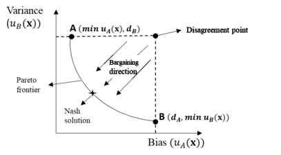
In this way, both the process variance and bias can guarantee the worst acceptable payoff. For example, process bias can take various values when variance is kept constant (e.g. ${\textstyle {\tilde {u}}_{B}({\boldsymbol {x}})}$) because multiple solution sets can result in the same variance value with different bias values. However, the process bias will choose the solution set that gives the smallest bias value, which is defined as the best response. Among the best responses for different situations, bias chooses the maximum as the disagreement point so that even if the agreement breaks down, the selected disagreement point is guaranteed. As demonstrated by Figure 3, the convex curve represents all of the Pareto optimal solutions. Each point on the curve can be understood as the best response for bias when variance chooses a specific value, and vice versa. For example, when the process bias takes the minimum value at point A, the best response for variance is the corresponding variance value, since other variance values would be either dominated or infeasible. In that case, the disagreement point can be calculated by minimizing only one object (process variance or bias). When the process bias is minimized, a corresponding variance value can be calculated, and vice versa. These calculated values are treated as the disagreement point payoff. In mathematical form, this is:

${\textstyle \left\{{d}_{A}={u}_{A}({\boldsymbol {x}})\right\}}$

(10)

and

${\textstyle \left\{{d}_{B}={u}_{B}({\boldsymbol {x}})\,\right\}}$

(11)

It is obvious that B ( ${\textstyle {d}_{A}\,,\,{minu}_{B}({\boldsymbol {x}})}$) and A ( ${\textstyle min{u}_{A}({\boldsymbol {x}}),\,{d}_{B})}$ are two Pareto optimal points. Thus, it is intuitively true that starting from the specified disagreement point, two players continue to bargain until an agreement is reached, this agreed solution point, marked as an asterisk, should be able to help the DM make a final decision.

FIGURE 3 Integration of the bargaining game into the trade-off problem between process bias and variance

Finally, the Nash bargaining solution function ${\textstyle Max\left({u}_{A}({\boldsymbol {x}})-\right.}$$\left.{d}_{A}\right)\left({u}_{B}({\boldsymbol {x}})-{d}_{B}\right)$ is used. In an RPD situation, the objective is to minimize both process bias and variance, so instead of the original constraint ${\textstyle {u}_{i}({\boldsymbol {x}})}$> ${\textstyle {d}_{i},\,i=}$$A,B$, a new constraint ${\textstyle {u}_{i}({\boldsymbol {x}})}$< ${\textstyle {d}_{i},\,i=}$$A,B$ is assumed. Applying the Nash bargaining solution function gives:

$max$ ${\textstyle \left({u}_{A}({\boldsymbol {x}})-{d}_{A}\right)\left({u}_{B}({\boldsymbol {x}})-\right.\left.{d}_{B}\right)}$ $s.t.$ ${u}_{A}({\boldsymbol {x}})\leq {d}_{A}$ ${\quad u}_{B}({\boldsymbol {x}})\leq {d}_{B}$ ${\boldsymbol {x}}\in \,X$

(12)

where

${\textstyle {u}_{A}\left({\boldsymbol {x}}\right)={\left({\hat {\mu }}({\boldsymbol {x}})-\tau \right)}^{2}}$

and

${\textstyle {u}_{B}\left({\boldsymbol {x}}\right)={\hat {\sigma }}^{2}({\boldsymbol {x}})}$

where ${\textstyle \,{d=(d}_{A},{d}_{B})}$ represents the disagreement point which specifies each player’s payoff when no agreement is reached (defined in Equations 10 and 11). ${\textstyle {\hat {\mu }}\left({\boldsymbol {x}}\right)}$ and ${\textstyle {\hat {\sigma }}^{2}\left({\boldsymbol {x}}\right)}$ are the mean and variance RSM estimated functions (shown in Equation 14 and 15), respectively. ${\textstyle \tau }$ represents the target value

${\textstyle {\hat {\mu }}\left({\boldsymbol {x}}\right){\mathit {\boldsymbol {=\,}}}{\alpha }_{0}{\mathit {\boldsymbol {+\,}}}{\boldsymbol {x}}^{T}{\boldsymbol {\alpha }}_{\boldsymbol {1}}{\mathit {\boldsymbol {+\,}}}{\boldsymbol {x}}^{T}{\boldsymbol {A\,x}}}$

(14)

where

${\textstyle {\boldsymbol {x}}=\left[\,{\begin{matrix}{x}_{1}\\{x}_{2}\\\,{\begin{matrix}\vdots \\{x}_{n-1}\\{x}_{n}\end{matrix}}\end{matrix}}\right]}$ , ${\textstyle {\mathit {\boldsymbol {\alpha }}}_{\mathit {\boldsymbol {1}}}=}$$\left[\,{\begin{matrix}{\hat {\alpha }}_{1}\\{\hat {\alpha }}_{2}\\\,{\begin{matrix}\vdots \\{\hat {\alpha }}_{n-1}\\{\hat {\alpha }}_{n}\end{matrix}}\end{matrix}}\right]$ , and

${\textstyle {\boldsymbol {A}}=}$$\,\left[{\begin{matrix}{\begin{matrix}{\hat {\alpha }}_{11}&{\hat {\alpha }}_{12}/2\\{\hat {\alpha }}_{12}/2&{\hat {\alpha }}_{22}\end{matrix}}&\cdots &{\begin{matrix}{\hat {\alpha }}_{1n}/2\\{\hat {\alpha }}_{2k}/2\end{matrix}}\\\vdots &\ddots &\vdots \\{\begin{matrix}{\hat {\alpha }}_{1n}/2&{\hat {\alpha }}_{2n}/2\end{matrix}}&\cdots &{\hat {\alpha }}_{nn}\end{matrix}}\right]$

${\textstyle \left\{{d}_{B}={u}_{B}({\boldsymbol {x}})\,\right\}}$

(11)

and ${\textstyle {\hat {\sigma }}^{2}\left({\boldsymbol {x}}\right){\mathit {\boldsymbol {=\,}}}{\beta }_{0}{\mathit {\boldsymbol {+\,}}}{{\boldsymbol {x}}^{\mathit {\boldsymbol {T}}}{\mathit {\boldsymbol {\beta }}}}_{\mathit {\boldsymbol {1}}}{\mathit {\boldsymbol {+\,}}}{\boldsymbol {x}}^{\mathit {\boldsymbol {T}}}{\boldsymbol {Bx}}}$ （15）

where

${\textstyle \,{\boldsymbol {x}}=\left[\,{\begin{matrix}{x}_{1}\\{x}_{2}\\\,{\begin{matrix}\vdots \\{x}_{n-1}\\{x}_{n}\end{matrix}}\end{matrix}}\right]}$ , ${\textstyle {\mathit {\boldsymbol {\beta }}}_{\mathit {\boldsymbol {1}}}=}$$\,\left[{\begin{matrix}{\hat {\beta }}_{1}\\{\begin{matrix}{\hat {\beta }}_{2}\\\vdots \end{matrix}}\\{\begin{matrix}{\hat {\beta }}_{n-1}\\{\hat {\beta }}_{n}\end{matrix}}\end{matrix}}\right]$ , and ${\textstyle {\boldsymbol {B}}=}$$\,\left[{\begin{matrix}{\begin{matrix}{\hat {\beta }}_{11}&{\hat {\beta }}_{12}/2\\{\hat {\beta }}_{12}/2&{\hat {\beta }}_{22}\end{matrix}}&\cdots &{\begin{matrix}{\hat {\beta }}_{1n}/2\\{\hat {\beta }}_{2n}/2\end{matrix}}\\\vdots &\ddots &\vdots \\{\begin{matrix}{\hat {\beta }}_{1n}/2&{\hat {\beta }}_{2n}/2\end{matrix}}&\cdots &{\hat {\beta }}_{nn}\end{matrix}}\right]$

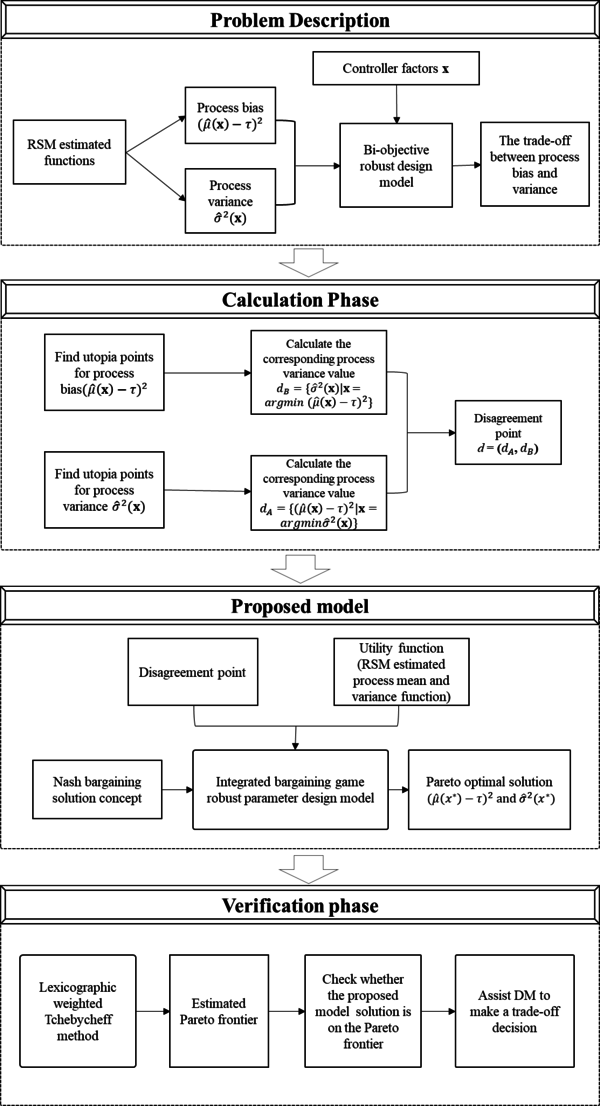
Here, the constraint of ${\textstyle {u}_{i}({\boldsymbol {x}})}$≤ ${\textstyle {d}_{i},\,\,i=}$$A,B$ ensures that the approaching agreement point payoff will be at least as good as the disagreement point payoff. Otherwise, there is no reason for the negotiation. The integrated process is summarized in Figure 4.

FIGURE 4: Illustration of the integration of bargaining game into RPD

5. Numerical illustrations and sensitivity analysis

5.1 Numerical example 1

Two numerical examples are conducted to study the efficiency of our proposed method. Example 1 investigates the relationship between the coating thickness of bare silicon wafers (y) and three controller variables, mould temperature ${\textstyle ({x}_{1})}$, injection flow rate ${\textstyle ({x}_{2})}$, and cooling rate ${\textstyle {(x}_{3})}$. This example was also discussed by Shin and Cho.46 A central composite design with ${\textstyle {2}^{3}\,}$ factorial design points and three replications was conducted, and details of the experimental data with coded value are shown in Table 1:

TABLE 1 Data for numerical example 1

Experiments number	${\boldsymbol {x}}_{\mathit {\boldsymbol {1}}}$	${\boldsymbol {x}}_{\mathit {\boldsymbol {2}}}$	${\boldsymbol {x}}_{\mathit {\boldsymbol {3}}}$	${\boldsymbol {y}}_{\mathit {\boldsymbol {1}}}$	${\boldsymbol {y}}_{\mathit {\boldsymbol {2}}}$	${\boldsymbol {y}}_{\mathit {\boldsymbol {3}}}$	${\boldsymbol {y}}_{\mathit {\boldsymbol {4}}}$	${\overline {\mathit {\boldsymbol {y}}}}$	${\mathit {\boldsymbol {\sigma }}}$
1	-1	-1	-1	76.30	80.50	77.70	81.10	78.90	2.28
2	1	-1	-1	79.10	81.20	78.80	79.60	79.68	1.07
3	-1	1	-1	82.50	81.50	79.50	80.90	81.10	1.25
4	1	1	-1	72.30	74.30	75.70	72.70	73.75	1.56
5	-1	-1	1	70.60	72.70	69.90	71.50	71.18	1.21
6	1	-1	1	74.10	77.90	76.20	77.10	76.33	1.64
7	-1	1	1	78.50	80.00	76.20	75.30	77.50	2.14
8	1	1	1	84.90	83.10	83.90	83.50	83.85	0.77
9	-1.682	0	0	74.10	71.80	72.50	71.90	72.58	1.06
10	1.682	0	0	76.40	78.70	79.20	79.30	78.40	1.36
11	0	-1.682	0	79.20	80.70	81.00	82.30	80.80	1.27
12	0	1.682	0	77.90	76.40	76.90	77.40	77.15	0.65
13	0	0	-1.682	82.40	82.70	82.60	83.10	82.70	0.29
14	0	0	1.682	79.70	82.40	81.00	81.20	81.08	1.11
15	0	0	0	70.40	70.60	70.80	71.10	70.73	0.30
16	0	0	0	70.90	69.70	69.00	69.90	69.88	0.78
17	0	0	0	70.70	71.90	71.70	71.20	71.38	0.54
18	0	0	0	70.20	71.00	71.50	70.40	70.78	0.59
19	0	0	0	71.50	71.10	71.20	70.00	70.95	0.66
20	0	0	0	71.00	70.40	70.90	69.90	70.55	0.51

The estimated response functions are:

${\textstyle {\left(\mu \left({\boldsymbol {x}}\right)-\tau \right)}^{2}=}$${\left(72.21+0.59{x}_{1}-0.35{x}_{2}-0.01{x}_{3}+0.28{{x}_{1}}^{2}+1.29{{x}_{2}}^{2}+1.85{{x}_{3}}^{2}+0.09{x}_{1}{x}_{2}+1.66{x}_{1}{x}_{3}+1.51{x}_{2}{x}_{3}-71.14\right)}^{2}$ （16）

${\textstyle {\begin{matrix}\sigma \left({\boldsymbol {x}}\right)=2.55+0.38{x}_{1}-0.43{x}_{2}+0.56{x}_{3}+0.49{{x}_{1}}^{2}+0.61{{x}_{2}}^{2}+0.85{{x}_{3}}^{2}\\-0.47{x}_{1}{x}_{2}+0.72{x}_{1}{x}_{3}-0.12{x}_{2}{x}_{3}\end{matrix}}}$ （17）

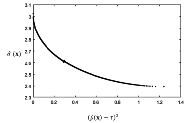
First, taking process bias as player A and standard deviation as player B, the utopia points for the two are (0, 3.1504) and (2.3948, 1.2398), respectively. The disagreement point is d= ( ${\textstyle {d}_{\mathit {\boldsymbol {A}}}}$, ${\textstyle {d}_{\mathit {\boldsymbol {B\,}}})=}$(1.2398, 3.1504) where ${\textstyle {d}_{A}}$ is calculated by minimizing the standard deviation ( ${\textstyle \sigma ({\boldsymbol {x}})}$) and obtaining the corresponding process bias ( ${\textstyle {\left({\hat {\mu }}\left({\boldsymbol {x}}\right)-\tau \right)}^{2})}$ value as ${\textstyle \,{d}_{A}}$. Similarly, ${\textstyle {d}_{B{\mathit {\boldsymbol {\,}}}}}$is calculated by minimizing the process bias and obtaining the corresponding standard deviation value. Then, the optimization problem can be solved using Formula (12) under the constraints of (13) and ${\textstyle \sum _{l=1}^{3}{{x}_{l}}^{2}\leq 3}$.

The solution is calculated by using the MATLAB R2016a built-in optimization tool fmincon, and the results are ${\textstyle {\left({\hat {\mu }}\left({\boldsymbol {x}}\right)-\tau \right)}^{2}=}$$0.2967$ and ${\textstyle \sigma \left({\boldsymbol {x}}\right)}$ = 2.6101. The lexicographic weighted Tchebycheff approach is adopted to check the efficiency of the result, and the Pareto frontier result is shown in Figure 5.

FIGURE 5 Pareto frontier for example 1 and solution plot of the proposed method

As shown in Figure 5, our Nash bargaining solution, which is plotted as a star, is on the Pareto frontier. When using the concept from bargaining game theory, the interaction between process bias and variance is incorporated and a unique tradeoff result is identified. This result could provide useful information to help DMs choose from abundant available non-dominated points.

5.2 Numerical example 2

The second example is from Cho and Park;47 it is an unbalanced data case that studies the relationship between coating thickness (y), mould temperature ( ${\textstyle {x}_{1}}$), and injection flow rate ( ${\textstyle {x}_{2}}$). The authors used a ${\textstyle {3}^{2}}$ factorial design with three levels, -1, 0, and +1, respectively. The detailed data is shown in Table 2:

TABLE 2 Data for numerical example 2

Experiments number	${\mathit {\boldsymbol {x}}}_{\boldsymbol {1}}$	${\mathit {\boldsymbol {x}}}_{\boldsymbol {2}}$	${\mathit {\boldsymbol {y}}}_{\boldsymbol {1}}$	${\mathit {\boldsymbol {y}}}_{\boldsymbol {2}}$	${\mathit {\boldsymbol {y}}}_{\boldsymbol {3}}$	${\mathit {\boldsymbol {y}}}_{\boldsymbol {4}}$	${\mathit {\boldsymbol {y}}}_{\boldsymbol {5}}$	${\mathit {\boldsymbol {y}}}_{\boldsymbol {6}}$	${\mathit {\boldsymbol {y}}}_{\boldsymbol {7}}$	${\overline {\mathit {\boldsymbol {y}}}}$	${\mathit {\boldsymbol {\sigma }}}^{\mathit {\boldsymbol {2}}}$
1	-1	-1	84.3	57.0	56.5					65.93	253.06
2	0	-1	75.7	87.1	71.8	43.8	51.6			66.00	318.28
3	1	-1	65.9	47.9	63.3					59.03	94.65
4	-1	0	51.0	60.1	69.7	84.8	74.7			68.06	170.35
5	0	0	53.1	36.2	61.8	68.6	63.4	48.6	42.5	53.46	139.89
6	1	0	46.5	65.9	51.8	48.4	64.4			55.40	83.11
7	-1	1	65.7	79.8	79.1					74.87	63.14
8	0	1	54.4	63.8	56.2	48.0	64.5			57.38	47.54
9	1	1	50.7	68.3	62.9					60.63	81.29

Cho and Park (2005) used the weighted least square (WLS) method to estimate the mean and variance function, as:

${\textstyle {\hat {\mu }}\left({\boldsymbol {x}}\right)=55.08-5.76{x}_{1}-}$$0.52{x}_{2}+5.51{x}_{1}^{2}+5.47{x}_{2}^{2}-1.84{x}_{1}{x}_{2}$ （18）

${\textstyle {\hat {\sigma }}^{2}\left({\boldsymbol {x}}\right)=154.26-}$$39.34{x}_{1}-93.09{x}_{2}-38.31{x}_{1}^{2}+17.81{x}_{2}^{2}+44.14{x}_{1}{x}_{2}$ （19）

Modifying the mean function as squared bias:

${\textstyle {({\hat {\mu }}({\boldsymbol {x}})-\tau )}^{2}={((55.08-5.76{x}_{1}-0.52{x}_{2}+5.51{x}_{1}^{2}+5.47{x}_{2}^{2}-1.84{x}_{1}{x}_{2})-50)}^{2}}$ （20）

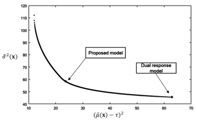
Applying the same logic as in example 1, the process bias is player A and variance as player B. First, the ranges for bias and variance are calculated using the built-in optimization tool called fmincon; these are [12.0508, 420.25] and [45.53, 310.39], respectively. Second, the disagreement points are computed as ${\textstyle {d}_{A}}$ =63.0436 and ${\textstyle {d}_{B}}$=112.0959. Applying function (12) while taking function (13) and ${\textstyle -}$$1<{x}_{k}<1,\,k=1,\,2$ as constraints gives the ultimate answer, ${\textstyle {({\hat {\mu }}({\boldsymbol {x}})-\tau )}^{2}}$=23.6526, ${\textstyle {\hat {\sigma }}^{2}\left({\boldsymbol {x}}\right)=}$ 58.3974. When this result is compared with that of Cho and Park ⁴⁶ which used a dual response model with WLS estimation method, our result outperforms theirs in terms of MSE (Table 3).

TABLE 3 Optimal solution comparison

	${x}_{1}^{\ast }$	${x}_{2}^{\ast }$	$\left|{\hat {\mu }}{\mathit {\boldsymbol {(}}}{\boldsymbol {x}}{\mathit {\boldsymbol {)-}}}\tau \right|$	${\hat {\sigma }}^{2}{\mathit {\boldsymbol {(}}}{\boldsymbol {x}}{\mathit {\boldsymbol {)}}}$	MSE
Dual response model with WLS	0.998	0.998	7.93	45.66	108.48
Proposed model	1.000	0.4440	4.8606	58.3974	82.023

By applying the lexicographic weighted Tchebycheff approach, we can obtain all non-dominated points that form the Pareto optimal frontier (Figure 6). Again, the Nash bargaining solution is on the Pareto frontier, which may provide a valuable suggestion for the trade-off problem.

FIGURE 6 Pareto frontier for example 2 and solution plot of the proposed method

5.3 Sensitivity analysis for numerical example 1

In this section, the effect of different disagreement point values will be investigated. In example 1, the disagreement point is d= ( ${\textstyle {d}_{A}}$, ${\textstyle {d}_{B{\mathit {\boldsymbol {\,}}}})=}$ (1.2398, 3.1504). Now, while the value of ${\textstyle {d}_{B{\mathit {\boldsymbol {\,}}}}}$is fixed at 3.1504, the value of ${\textstyle {d}_{A{\mathit {\boldsymbol {\,}}}}}$ is changed in steps of 10% (both increase and decrease) and the resulting changes in process bias and variance are investigated.

TABLE 4 Example 1 sensitivity analysis; ${\textstyle {d}_{A}}$ is increased and decreased by 10%

${d}_{A}$	${d}_{B}$	${{\mathit {\boldsymbol {((}}}{\hat {\mu }}\left({\boldsymbol {x}}\right){\mathit {\boldsymbol {-}}}t{\mathit {\boldsymbol {)}}}}^{\mathit {\boldsymbol {2}}}-$${d}_{A}{\boldsymbol {)\ast (}}{\hat {\sigma }}\left({\boldsymbol {x}}\right)-$${d}_{B}{\mathit {\boldsymbol {)}}}$	x	${{\boldsymbol {(}}\mu \left({\boldsymbol {x}}\right){\boldsymbol {-}}\tau {\boldsymbol {)}}}^{\boldsymbol {2}}$	$\sigma \left({\boldsymbol {x}}\right)$
0.6589	3.1504	0.2218	[-1.0281 -0.0159 0.3253]	0.157	2.7085
0.7321	3.1504	0.2547	[-1.0017 -0.0078 0.3107]	0.1753	2.6930
0.8134	3.1504	0.2925	[-0.9739 0.0007 0.2953]	0.1953	2.6771
0.9038	3.1504	0.3361	[-0.9445 0.0098 0.2790]	0.2174	2.6608
1.0042	3.1504	0.3861	[-0.9137 0.0193 0.2619]	0.2416	2.6441
1.1158	3.1504	0.4435	[-0.8813 0.0293 0.2438]	0.2680	2.6272
1.2398	3.1504	0.5095	[-0.8473 0.0399 0.2248]	0.2967	2.6101
1.3638	3.1504	0.5775	[-0.8153 0.0499 0.2069]	0.3248	2.5946
1.5002	3.1504	0.6543	[-0.7820 0.0603 0.1881]	0.3549	2.5791
1.6502	3.1504	0.7412	[-0.7475 0.0711 0.1687]	0.3869	2.5637
1.8152	3.1504	0.8393	[-0.7120 0.0824 0.1486]	0.4209	2.5484
1.9967	3.1504	0.9499	[-0.6754 0.0939 0.1278]	0.4567	2.5335
2.1964	3.1504	1.0746	[-0.6381 0.1058 0.1065]	0.4942	2.5191
2.4160	3.1504	1.2148	[-0.6002 0.1180 0.0847]	0.5331	2.5052

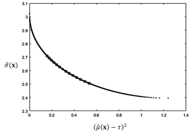
As shown in Table 4, if only ${\textstyle {d}_{A}}$ increases, the final solution value of ${\textstyle {({\hat {\mu }}({\boldsymbol {x}})-\tau )}^{2}}$ increases while ${\textstyle {\hat {\sigma }}\left({\boldsymbol {x}}\right)}$ decreases. All of the calculated results are plotted as circles and compared with the Pareto frontier generated by the lexicographic weighted Tchebycheff method. Clearly, all of the points are on the Pareto frontier, as shown in Figure 7.

FIGURE 7 A plot of all calculated solution points for numerical example 1 when ${\textstyle {d}_{A}}$ is changed by 10%

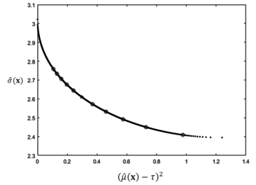
On the contrary, if ${\textstyle {d}_{A}}$ is treated as a constant and ${\textstyle {d}_{B}}$ is changed by 5% each time, the data is transformed as summarized in Table 5 and Figure 8.

TABLE 5 Example 1 sensitivity analysis; ${\textstyle {d}_{B}}$ is increased and decreased by 5%

${d}_{A}$	${d}_{B}$	${{\mathit {\boldsymbol {((}}}{\hat {\mu }}\left({\boldsymbol {x}}\right){\mathit {\boldsymbol {-}}}t{\mathit {\boldsymbol {)}}}}^{\mathit {\boldsymbol {2}}}-$${d}_{A}{\boldsymbol {)\ast (}}{\hat {\sigma }}\left({\boldsymbol {x}}\right)-$${d}_{B}{\mathit {\boldsymbol {)}}}$	x	${{\boldsymbol {(}}{\hat {\mu }}\left({\boldsymbol {x}}\right){\boldsymbol {-}}\tau {\boldsymbol {)}}}^{\boldsymbol {2}}$	${\hat {\sigma }}\left({\boldsymbol {x}}\right)$
1.2398	2.4377	0.0076	[-0.2082 0.2495 -0.1539]	0.9764	2.4089
1.2398	2.5660	0.0592	[-0.4198 0.1770 -0.0212]	0.7286	2.4501
1.2398	2.7011	0.1394	[-0.5607 0.1307 0.0618]	0.5746	2.4916
1.2398	2.4832	0.2425	[-0.6726 0.0948 0.1262]	0.4595	2.5324
1.2398	2.9929	0.3664	[-0.7666 0.0651 0.1795]	0.3690	2.5721
1.2398	3.1504	0.5095	[-0.8473 0.0399 0.2248]	0.2967	2.6101
1.2398	3.3079	0.6626	[-0.9141 0.0192 0.2621]	0.2412	2.6444
1.2398	3.4733	0.8316	[-0.9727 0.0011 0.2946]	0.1962	2.6764
1.2398	3.6470	1.0162	[-1.0241 -0.0147 0.3231]	0.1597	2.7061
1.2398	3.8293	1.2159	[-1.0692 -0.0285 0.3480]	0.1303	2.7334
1.2398	4.0208	1.4308	[-1.1088 -0.0406 0.3698]	0.1065	2.7583

FIGURE 8 A plot of all calculated solution points for numerical example 1 when ${\textstyle {d}_{B}}$ is changed by 5%

As demonstrated by Table 5, solution value of ${\textstyle {({\hat {\mu }}({\boldsymbol {x}})-\tau )}^{2}}$ declines while ${\textstyle \,{\hat {\sigma }}\left({\boldsymbol {x}}\right)}$ grows if ${\textstyle {d}_{B}}$ is increased and ${\textstyle {d}_{A}}$ is kept constant. However, all of the solution points are still on the Pareto frontier, as shown in Figure 8.

5.4 Sensitivity analysis for numerical example 2

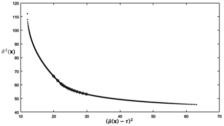
Applying the same logic for example 2, ${\textstyle {d}_{B}}$ is kept constant as ${\textstyle {d}_{A}}$ is changed by 10%. Table 6 exhibits the effect of changes in ${\textstyle {d}_{A}}$, and Figure 9 demonstrates the efficiency of the calculated solutions.

Table 6 Example 2 sensitivity analysis; ${\textstyle {d}_{A}}$ is increased and decreased by 10%

${d}_{A}$	${d}_{B}$	${{\mathit {\boldsymbol {((}}}{\hat {\mu }}\left({\boldsymbol {x}}\right){\mathit {\boldsymbol {-}}}\tau {\mathit {\boldsymbol {)}}}}^{\mathit {\boldsymbol {2}}}-$${d}_{A}{\boldsymbol {)\ast (}}{\hat {\sigma }}^{2}\left({\boldsymbol {x}}\right)-$${d}_{B}{\mathit {\boldsymbol {)}}}$	x	${{\boldsymbol {(}}{\hat {\mu }}\left({\boldsymbol {x}}\right){\boldsymbol {-}}\tau {\boldsymbol {)}}}^{\boldsymbol {2}}$	${\hat {\sigma }}^{\mathit {\boldsymbol {2}}}\left({\boldsymbol {x}}\right)$
37.2266	112.0959	790.0487	[ 0.9510 0.3554]	19.9778	66.2928
41.3629	112.0959	986.2591	[0.9813 0.3624]	21.2437	63.0751
45.9588	112.0959	1218.3	[1.0000 0.3751]	22.2248	60.7647
51.0653	112.0959	1482.5	[1.0000 0.3978]	22.6267	59.9662
56.7392	112.0959	1780.6	[1.000 0.4208]	23.0925	59.1766
63.0436	1120959	2116.7	[1.0000 0.4440]	23.6256	58.3974
69.3480	112.0959	2457.5	[1.0000 0.4653]	24.1686	57.7026
76.2828	112.0959	2837.1	[1.0000 0.4867]	24.7721	57.0185
83.9110	112.0959	3259.8	[1.0000 0.5083]	25.4386	56.346
92.3021	112.0959	3730.5	[1.0000 0.5300]	26.1709	55.686
101.5323	112.0959	4254.2	[1.0000 0.5518]	26.9716	55.0393
111.6856	112.0959	4836.8	[1.0000 0.5738]	27.8435	54.407
122.8541	112.0959	5484.6	[1.0000 0.5958]	28.7892	53.7896
135.1396	112.0959	6204.7	[1.0000 0.6179]	29.8115	53.1879

Figure 9 A plot of all calculated solution points for numerical example 2 when ${\textstyle {d}_{A}}$ is changed by10%

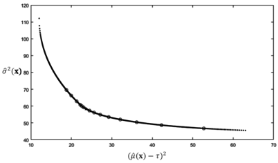
Likewise, ${\textstyle {d}_{A}}$ is kept constant while ${\textstyle {d}_{B}}$ is changed by 10%. The altered data are summarized in Table 7 and plotted in Figure 10.

Table 7 Example 2 sensitivity analysis; ${\textstyle {d}_{B}}$ is increased and decreased by 10%

${d}_{A}$	${d}_{B}$	${{\mathit {\boldsymbol {((}}}{\hat {\mu }}\left({\boldsymbol {x}}\right){\mathit {\boldsymbol {-}}}\tau {\mathit {\boldsymbol {)}}}}^{\mathit {\boldsymbol {2}}}-$${d}_{A}{\boldsymbol {)\ast (}}{\hat {\sigma }}^{\mathit {\boldsymbol {2}}}\left({\boldsymbol {x}}\right)-$${d}_{B}{\mathit {\boldsymbol {)}}}$	x	${{\boldsymbol {(}}{\hat {\mu }}\left({\boldsymbol {x}}\right){\boldsymbol {-}}\tau {\boldsymbol {)}}}^{\boldsymbol {2}}$	${\hat {\sigma }}^{\mathit {\boldsymbol {2}}}\left({\boldsymbol {x}}\right)$
63.0436	48.2536	15.4253	[1.0000 0.9166]	52.7429	46.7561
63.0436	53.6151	102.0493	[1.0000 0.8094]	42.2936	48.6971
63.0436	59.5724	245.6339	[1.0000 0.7284]	36.1567	50.4366
63.0436	66.1915	438.1362	[1.0000 0.6620]	32.0892	52.0372
63.0436	73.5461	677.0693	[1.0000 0.6055]	29.2313	53.5218
63.0436	81.7179	962.4337	[1.0000 0.5567]	27.1579	54.8985
63.0436	90.7977	1295.7	[1.0000 0.5140]	25.6262	56.1698
63.0436	100.8863	1679.3	[1.0000 0.4767]	24.4832	57.3359
63.0436	112.0959	2116.7	[1.0000 0.4440]	23.6256	58.3974
63.0436	123.3066	2562.1	[1.0000 0.4181]	23.0342	59.2691
63.0436	135.6372	3058.4	[1.0000 0.3951]	22.5764	60.0593
63.0436	149.2010	3609.9	[1.0000 0.3748]	22.2214	60.7721
63.0436	164.1211	4223.7	[0.9829 0.3628]	21.3147	62.9025
63.0436	180.5332	4919.9	[0.9512 0.3554]	19.9864	66.2698
63.0436	198.5865	5708.3	[0.9199 0.3472]	18.7938	69.5842

FIGURE 10 A plot of all calculated solution points for numerical example 2 when ${\textstyle {d}_{B}}$ is changed by 10%

In conclusion, in both cases, an increase in the value of ${\textstyle {d}_{i}}$ will increase the corresponding bargaining solution value. In other words, an increase in ${\textstyle {d}_{A}}$ will increase the process bias result, and an increase in ${\textstyle {d}_{B}}$ will raise the variance. The result also makes sense from the perspective of game theory since it can be explained as disagreement point monotonicity48 which can be defined as:

For two points, ${\textstyle \,d=\left({d}_{A},\,{\,d}_{B}\right)}$ and ${\textstyle \,{d}^{'}=}$$\left({{d}_{A}}^{'},\,{{\,d}_{B}}^{'}\right)$ , ${\textstyle if\,{d}_{i}^{'}\geq {d}_{i},\,{d}_{j}^{,}=}$${d}_{j},\,then\,{f}_{i}\left(U,{d}^{'}\right)\geq {f}_{i}\left(U,d\right)\,;\,j\not =i,\,and\,i,j\in \lbrace A,\,B\rbrace$ .

where ${\textstyle {f}_{i}\left(U,{d}^{'}\right)}$ and ${\textstyle {f}_{i}\left(U,d\right)}$ is the solution payoff for player i after and before the incensement of his disagreement point payoff. ${\textstyle \,}$ More specifically, the more payoff a player demands for participation in an agreement, the more the player will get. Also, a gain achieved by one player comes at the expense of the other player. This is because when the agreement point is not an improvement for one player, any rational player would have no incentive to participate in the bargaining game. In the RPD case, the less ${\textstyle {d}_{i}}$ a player requires to join the agreement, the more the player is actually requiring since the objective is to minimize objective functions in contrast to the general bargaining game which seeks to maximize the payoff.

6. CONCLUSION AND FURTHER DIRECTION

In the robust design model, when thinking of process bias and variance as a bi-objective problem, there is an intractable trade-off problem between them. In this paper, we proposed a bargaining game based RPD method to solve the trade-off problem by integrating the Nash bargaining solution concept and letting the two objectives (process bias and variance) “negotiate”, a unique, fair and efficient solution can be obtained that may help a DM to make a final choice. To inspect the efficiency of our obtained solutions the associated Pareto frontier was generated through the lexicographic weighted Tchebycheff method, and solution positions were visually confirmed. Two numerical examples were presented to illustrate the practicality of the proposed model. As solution figures (Figure 5 and 6) showed that our calculated final solution was on the Pareto frontier, which could provide a final solution for DM to solve the trade-off problem. Furthermore, a number of sensitivity studies were conducted to investigate the relationship between ${\textstyle {d}_{i}}$ and the final solution. This research illustrates the possibility of combining the concept of game theory with the process of RPD. In future, we wish to explore the n-player bargaining game and the asymmetry bargaining game to cover more complicated scenarios.

REFERENCE

1 Park, G. J., Lee, T. H., Lee, K. H., & Hwang, K. H. Robust design: an overview. AIAA journal, 44(1): 181-191, 2006.

2 Myers, W. R., Brenneman, W. A., & Myers, R. H. A dual-response approach to robust parameter design for a generalized linear model. Journal of Quality Technology, 37(2), 130-138, 2005.

3 Leon R.V., Shoemaker A.C., Kackar R.N. Performance Measures Independent of Adjustment: an Explanation and Extension of Taguchi’s Signal-To-Noise Ratios. Technometrics, 29(3), 253-265, 1987.

4 Box G. Signal-to-noise ratios, performance criteria, and transformations. Technometrics, 30(1): 1-17, 1988.

5 Nair V N, Abraham B, MacKay J, et al. Taguchi's parameter design: a panel discussion. Technometrics, 34(2): 127-161, 1992.

6 Tsui K L. An overview of Taguchi method and newly developed statistical methods for robust design. IIE Transactions, 24(5): 44-57, 1992.

7 Vining G G, Myers R H. Combining Taguchi and response surface philosophies: a dual response approach. Journal of quality technology, 22(1): 38-45, 1990.

8 Shoemaker A C, Tsui K L, Wu C F J. Economical experimentation methods for robust design. Technometrics, 33(4): 415-427, 1991.

9 Khattree R. Robust parameter design: A response surface approach. Journal of Quality Technology, 28(2): 187-198, 1996.

10 Pregibon, Daryl. Generalized linear models. The Annals of Statistics, 12(4): 1589–1596, 1984.

11 Lee S B, Park C. Development of robust design optimization using incomplete data. Computers & industrial engineering, 50(3): 345-356, 2006.

12 Cho B R, Park C. Robust design modeling and optimization with unbalanced data. Computers & industrial engineering, 48(2): 173-180, 2005.

13 Lin D K J, Tu W. Dual response surface optimization. Journal of Quality Technology, 27(1): 34-39, 1995.

14 Jayaram, J.S.R. and Ibrahim, Y. Multiple response robust design and yield maximization. International Journal of Quality & Reliability Management, 16(9): 826-837, 1999. https://doi.org/10.1108/02656719910274308

15 Köksoy O, Doganaksoy N. Joint optimization of mean and standard deviation using response surface methods. Journal of Quality Technology, 35(3): 239-252, 2003.

16 Shin S, Cho B R. Studies on a biobjective robust design optimization problem. IIE Transactions, 41(11): 957-968, 2009.

17 Shin, S., Hoang, T. T., Le, T. H., & Lee, M. Y.  A new robust design method using neural network. Journal of Nanoelectronics and Optoelectronics, 11(1): 68-78, 2016.

18 Picheral L, Hadj-Hamou K, Bigeon J. Robust optimization based on the Propagation of Variance method for analytic design models. International Journal of Production Research, 52(24): 7324-7338, 2014.

19 Mortazavi A, Azarm S, Gabriel S A. Adaptive gradient-assisted robust design optimization under interval uncertainty. Engineering Optimization, 45(11): 1287-1307, 2013.

20 Sohrabi M K, Azgomi H. A survey on the combined use of optimization methods and game theory. Archives of Computational Methods in Engineering, 27(1): 59-80, 2020.

21 Shoham Y. Computer science and game theory. Communications of the ACM, 51(8): 74-79, 2008.

22 Manshaei M H, Zhu Q, Alpcan T, et al. Game theory meets network security and privacy. ACM Computing Surveys (CSUR), 45(3): 1-39, 2013.

23 Pillai P S, Rao S. Resource allocation in cloud computing using the uncertainty principle of game theory. IEEE Systems Journal, 10(2): 637-648, 2014.

24 Lemaire J. An application of game theory: cost allocation. ASTIN Bulletin: The Journal of the IAA. 1984; 14(1): 61-81, 2014.

25 Barough A S, Shoubi M V, Skardi M J E. Application of game theory approach in solving the construction project conflicts. Procedia-Social and Behavioral Sciences, 58: 1586-1593, 2012.

26 Gale D, Kuhn H W, Tucker A W. Linear programming and the theory of game. Activity analysis of production and allocation, 13: 317-335, 1951.

27 Mangasarian O L, Stone H. Two-person nonzero-sum games and quadratic programming. Journal of mathematical analysis and applications, 9(3): 348-355, 1964.

28 Leboucher C, Shin H S, Siarry P, et al. Convergence proof of an enhanced particle swarm optimization method integrated with evolutionary game theory. Information Sciences, 346: 389-411, 2016.

29 Annamdas K K, Rao S S. Multi-objective optimization of engineering systems using game theory and particle swarm optimization. Engineering optimization, 41(8): 737-752, 2009.

30 Zamarripa, M. A., Aguirre, A. M., Méndez, C. A., & Espuña, A. Mathematical programming and game theory optimization-based tool for supply chain planning in cooperative/competitive environments. Chemical Engineering Research and Design, 91(8): 1588-1600, 2013.

31 Shi, Y., Xing, Y., Mou, C., & Kuang, Z. An optimization model based on game theory. Journal of Multimedia, 9(4): 583, 2014.

32 Matejaš J, Perić T. A new iterative method for solving multiobjective linear programming problem. Applied mathematics and computation, 243: 746-754, 2014.

33 Doudou, M., Barcelo-Ordinas, J. M., Djenouri, D., Garcia-Vidal, J., Bouabdallah, A., & Badache, N. Game theory framework for MAC parameter optimization in energy-delay constrained sensor networks. ACM Transactions on Sensor Networks (TOSN), 12(2), 1-35, 2016.

34 Dai, L., Tang, M., & Shin, S. Stackelberg game approach to a bi-objective robust design optimization. Revista Internacional de Métodos Numéricos para Cálculo y Diseño en Ingeniería, 37(4), 2021.

35 Myerson R B. Game Theory: Analysis of Conflict. Harvard University Press, Cambridge, MA. London England, 1991.

36 Goodpaster G. Rational decision-making in problem-solving negotiation: Compromise, interest-valuation, and cognitive error. Ohio St. J. on Disp. Resol. 8: 299, 1992.

37 Nash, J. F. The Bargaining Problem. Econometrica, 18(2):155-162, 1950.

38 Nash, J. F. Two-Person Cooperative Games. Econometrica, 21(1):128-140, 1953.

39 Rubinstein A. Perfect equilibrium in a bargaining model. Econometrica: Journal of the Econometric Society, 97-109, 1982.

40 Kalai E, Smorodinsky M. Other solutions to Nash's bargaining problem. Econometrica: Journal of the Econometric Society, 513-518, 1975.

41 Mandal W A. Weighted Tchebycheff optimization technique under uncertainty. Annals of Data Science, 1-23, 2020.

42 Dächert K, Gorski J, Klamroth K. An augmented weighted Tchebycheff method with adaptively chosen parameters for discrete bicriteria optimization problems. Computers & Operations Research, 39(12): 2929-2943, 2012.

43 Steuer R E, Choo E U. An interactive weighted Tchebycheff procedure for multiple objective programming. Mathematical programming, 26(3): 326-344, 1983.

44 Rausser G C, Swinnen J, Zusman P. Political power and economic policy: Theory, analysis, and empirical applications. Cambridge University Press, 2011.

45 Muthoo A. Bargaining theory with applications. Cambridge University Press, 1999.

46 Shin S, Cho B R. Robust design models for customer-specified bounds on process parameters. Journal of Systems Science and Systems Engineering, 15(1): 2-18, 2006.

47 Cho B R, Park C. Robust design modeling and optimization with unbalanced data. Computers & industrial engineering, 48(2): 173-180, 2005.

48 Thomson W. In: Handbook of game theory with economic applications. Cooperative models of Bargaining. 2: 1237-1284, 1994.