m (Cinmemj moved page Draft Samper 231103336 to Rossi et al 2019a) |
|||
| (60 intermediate revisions by the same user not shown) | |||
| Line 1,117: | Line 1,117: | ||
|- style="text-align: center; font-size: 75%;" | |- style="text-align: center; font-size: 75%;" | ||
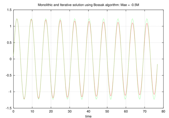
| colspan="1" | '''Figure 5:''' Comparison between exact and iterative coupled solutions using the Bossak algorithm. Bossak parameter = -0.1, period divided in 50 steps - Monolithic solution is dashed while the solution of iterative coupling is represented with a continuum line | | colspan="1" | '''Figure 5:''' Comparison between exact and iterative coupled solutions using the Bossak algorithm. Bossak parameter = -0.1, period divided in 50 steps - Monolithic solution is dashed while the solution of iterative coupling is represented with a continuum line | ||
| − | | | + | |} |
| − | | | + | {| |
|- style="text-align: center; font-size: 75%;" | |- style="text-align: center; font-size: 75%;" | ||
| − | |'''Notes:'''Bossak parameter = -0.1, period divided in 50 steps - Monolithic solution is dashed while the solution of iterative coupling is represented with a continuum line | + | |'''Notes:''' Bossak parameter = -0.1, period divided in 50 steps - Monolithic solution is dashed while the solution of iterative coupling is represented with a continuum line |
|} | |} | ||
==4 An improved iterative coupling procedure via a modified equations== | ==4 An improved iterative coupling procedure via a modified equations== | ||
| − | As discussed above the simple iterative strategy described in Section | + | As discussed above the simple iterative strategy described in Section [[#3 Iterative enhancement of the fractional step scheme|3]] may encounter convergence difficulties or even diverge depending on the features of the flow. Even relaxed iterative strategies may fail for complex FSI problems when the aeroelastic mass term becomes very important. |
This can be justified from an heuristic point of view by considering that most relaxation strategies perform a relaxation on the displacements term which in turn reflects on some form of control over the acceleration dependent contributions. Given the high dependency of the acceleration on small variations of the displacements, this turns out to be ineffective to control the (aeroelastic) mass-induced oscillations. | This can be justified from an heuristic point of view by considering that most relaxation strategies perform a relaxation on the displacements term which in turn reflects on some form of control over the acceleration dependent contributions. Given the high dependency of the acceleration on small variations of the displacements, this turns out to be ineffective to control the (aeroelastic) mass-induced oscillations. | ||
| Line 1,223: | Line 1,223: | ||
The parameter <math display="inline">\alpha </math> affects sensibly the condition for stability, hereby increasing the area of convergence. Any choice of the type <math display="inline">\alpha < \alpha ^{ex}</math> guarantees stability and monothonic convergence (<math display="inline">0<\frac{\alpha ^{ex}-\alpha }{1-\alpha }<1</math>) while the choice <math display="inline">\alpha ^{ex}<\alpha <\frac{1}{2}\alpha ^{ex}+\frac{1}{2}</math> guarantees stability but gives oscillatory convergence. Unfortunately the exact value for <math display="inline">\alpha </math> is not known. However Eqn([[#eq-69|69]]) ensures that the convergence is robust and that a rough estimation of the optimal value of <math display="inline">\alpha </math> is sufficient to ensure convergence. | The parameter <math display="inline">\alpha </math> affects sensibly the condition for stability, hereby increasing the area of convergence. Any choice of the type <math display="inline">\alpha < \alpha ^{ex}</math> guarantees stability and monothonic convergence (<math display="inline">0<\frac{\alpha ^{ex}-\alpha }{1-\alpha }<1</math>) while the choice <math display="inline">\alpha ^{ex}<\alpha <\frac{1}{2}\alpha ^{ex}+\frac{1}{2}</math> guarantees stability but gives oscillatory convergence. Unfortunately the exact value for <math display="inline">\alpha </math> is not known. However Eqn([[#eq-69|69]]) ensures that the convergence is robust and that a rough estimation of the optimal value of <math display="inline">\alpha </math> is sufficient to ensure convergence. | ||
| − | Let us make now some heuristic considerations on the properties of the modified equation approach proposed. The crucial point is that at every iteration we solve a problem that is different from the original one and which solution becomes increasingly similar to that of the original problem as the iterative process converges. Even at convergence, an error exists which implies that the solution found corresponds to a slightly different problem. The choice of an error tolerance therefore tell us how closely the modified equations will “mimic” the real problem. The key is however to guarantee “a priori” the stability of the coupled procedure while improving the accuracy as needed. Note that this is not the case for a general relaxation scheme. | + | Let us make now some heuristic considerations on the properties of the modified equation approach proposed. The crucial point is that at every iteration we solve a problem that is different from the original one and which solution becomes increasingly similar to that of the original problem as the iterative process converges. Even at convergence, an error exists which implies that the solution found corresponds to a slightly different problem. The choice of an error tolerance therefore tell us how closely the modified equations will “mimic” the real problem. The key is however to guarantee ''“a priori”'' the stability of the coupled procedure while improving the accuracy as needed. Note that this is not the case for a general relaxation scheme. |
===4.1 Estimating alpha=== | ===4.1 Estimating alpha=== | ||
| Line 1,231: | Line 1,231: | ||
Several possibilities exist for the practical estimation of a coefficient <math display="inline">\alpha </math> to be used in improving the convergence of the coupled solver. A good estimation could be derived by physical reasoning or by considering the actual choice of the flow solver. | Several possibilities exist for the practical estimation of a coefficient <math display="inline">\alpha </math> to be used in improving the convergence of the coupled solver. A good estimation could be derived by physical reasoning or by considering the actual choice of the flow solver. | ||
| − | An alternative procedure, which makes use exclusively of the data at different iterations is derived next for the non-scalar case. A general iterative scheme for the estimation of such parameter may lead to the use of a different estimate of <math display="inline">\alpha </math> at each iteration | + | An alternative procedure, which makes use exclusively of the data at different iterations is derived next for the non-scalar case. A general iterative scheme for the estimation of such parameter may lead to the use of a different estimate of <math display="inline">\alpha </math> at each iteration “<math>i</math>”. If we assume however the use of a constant <math display="inline">\alpha ^i</math> through the iteration process, the application of Eqn([[#eq-67|67]]) to two successive iterations gives |
{| class="formulaSCP" style="width: 100%; text-align: left;" | {| class="formulaSCP" style="width: 100%; text-align: left;" | ||
| Line 1,312: | Line 1,312: | ||
|} | |} | ||
| style="width: 5px;text-align: right;white-space: nowrap;" | (75) | | style="width: 5px;text-align: right;white-space: nowrap;" | (75) | ||
| − | |||
| − | |||
| − | |||
| − | |||
| − | |||
| − | |||
| − | |||
| − | |||
| − | |||
| − | |||
| − | |||
| − | |||
| − | |||
| − | |||
| − | |||
| − | |||
|} | |} | ||
| Line 1,342: | Line 1,326: | ||
|} | |} | ||
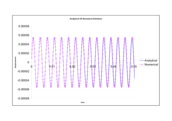
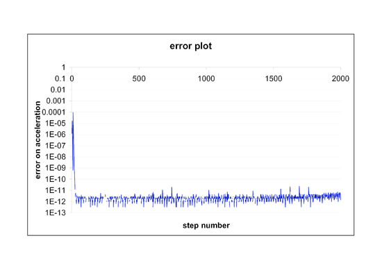
| − | Fig. [[#img- | + | Fig. [[#img-6|6]] shows a comparison between the exact and analytical results. Convergence is obtained in two iterations except during the first three time steps. A plot of the error norm <math display="inline">\left\| \ddot{x} ^{i+1}- \ddot{x} ^i\right\|</math> is given in Fig. [[#img-7|7]] |
| − | <div id='img- | + | <div id='img-6'></div> |
{| class="floating_imageSCP" style="text-align: center; border: 1px solid #BBB; margin: 1em auto; width: 100%;max-width: 100%;" | {| class="floating_imageSCP" style="text-align: center; border: 1px solid #BBB; margin: 1em auto; width: 100%;max-width: 100%;" | ||
|- | |- | ||
| − | |[[Image:Draft_Samper_231103336- | + | |[[Image:Draft_Samper_231103336-AnalyticalVsNumerical.png|600px|Comparison between analytical and numerical solution for the cube model problem]] |
|- style="text-align: center; font-size: 75%;" | |- style="text-align: center; font-size: 75%;" | ||
| − | | colspan="1" | '''Figure | + | | colspan="1" | '''Figure 6:''' Comparison between analytical and numerical solution for the cube model problem |
|} | |} | ||
| − | <div id='img- | + | <div id='img-7'></div> |
{| class="floating_imageSCP" style="text-align: center; border: 1px solid #BBB; margin: 1em auto; width: 100%;max-width: 100%;" | {| class="floating_imageSCP" style="text-align: center; border: 1px solid #BBB; margin: 1em auto; width: 100%;max-width: 100%;" | ||
|- | |- | ||
| − | |[[Image:Draft_Samper_231103336- | + | |[[Image:Draft_Samper_231103336-errorplot.png|550px|Acceleration error for the simple cube benchmark scheme]] |
|- style="text-align: center; font-size: 75%;" | |- style="text-align: center; font-size: 75%;" | ||
| − | | colspan="1" | '''Figure | + | | colspan="1" | '''Figure 7:''' Acceleration error for the simple cube benchmark scheme |
|} | |} | ||
==5 Restrictor Flap== | ==5 Restrictor Flap== | ||
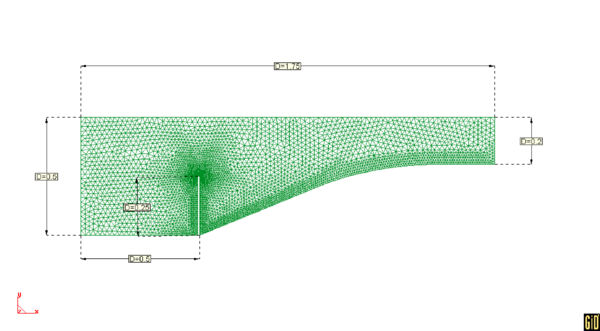
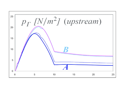
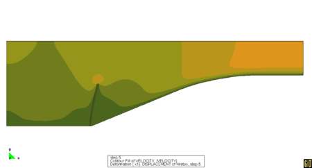
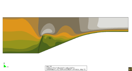
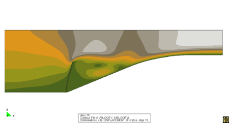
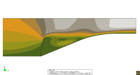
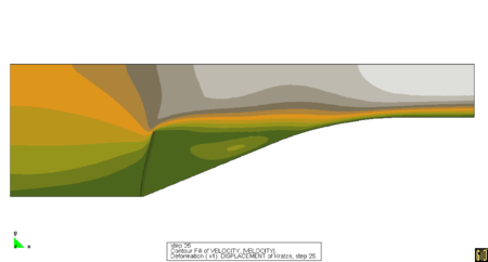
| − | This test was proposed by Wall and Mok <span id='citeF-1'></span>[[#cite-1|[1]]] and Mok <span id='citeF-2'></span>[[#cite-2|[2]]], as a challenging test for the stability of solution algorithm procedures. The geometry is described in Fig. [[#img- | + | This test was proposed by Wall and Mok <span id='citeF-1'></span>[[#cite-1|[1]]] and Mok <span id='citeF-2'></span>[[#cite-2|[2]]], as a challenging test for the stability of solution algorithm procedures. The geometry is described in Fig. [[#img-8|8]]. The data used for the analysis are <math display="inline">\rho _F = 956 Kg/m^3</math>, <math display="inline">\mu = 0.145 Kg/ms</math>, <math display="inline">\rho _S = 1500 Kg/m^3</math>, <math display="inline">E = 2.3 MPa</math>, <math display="inline">\nu = 2.3 MPa</math>. The resulting pressure histories are shown in Fig. [[#img-9|9]] and directly compared with the results of the literature. The frames shown in Fig. [[#img-10|10]] show the evolution of the coupled fluid-structure deformation and compare well with the results of the same example as reported in Mok <span id='citeF-2'></span>[[#cite-2|[2]]]. A second order fractional step solver is used for solving the problem. The resulting pressure histories are shown in Fig. [[#img-9|9]] and directly compared with the results of the literature |
| − | <div id='img- | + | <div id='img-8'></div> |
| − | + | ||
| − | + | ||
| − | + | ||
| − | + | ||
| − | + | ||
| − | + | ||
{| class="floating_imageSCP" style="text-align: center; border: 1px solid #BBB; margin: 1em auto; width: 100%;max-width: 100%;" | {| class="floating_imageSCP" style="text-align: center; border: 1px solid #BBB; margin: 1em auto; width: 100%;max-width: 100%;" | ||
|- | |- | ||
| − | |[[Image:Draft_Samper_231103336- | + | |[[Image:Draft_Samper_231103336-mesh_restrictor.png|600px|Restrictor flap - mesh of 7928 elements]] |
| − | + | ||
|- style="text-align: center; font-size: 75%;" | |- style="text-align: center; font-size: 75%;" | ||
| − | + | | colspan="1" | '''Figure 8:''' Restrictor flap - mesh of 7928 elements | |
| − | + | ||
| − | + | ||
| − | + | ||
| − | + | ||
| − | + | ||
| − | + | ||
| − | + | ||
| − | + | ||
| − | | colspan=" | + | |
| − | + | ||
| − | + | ||
| − | + | ||
| − | + | ||
|} | |} | ||
| − | <div id='img- | + | <div id='img-9'></div> |
{| class="floating_imageSCP" style="text-align: center; border: 1px solid #BBB; margin: 1em auto; width: 100%;max-width: 100%;" | {| class="floating_imageSCP" style="text-align: center; border: 1px solid #BBB; margin: 1em auto; width: 100%;max-width: 100%;" | ||
|- | |- | ||
| − | |[[Image:Draft_Samper_231103336- | + | |[[Image:Draft_Samper_231103336-pressure_comparison.png|400px|Pressure vs time at mid-height (A) and at the tip (B)]] |
|- style="text-align: center; font-size: 75%;" | |- style="text-align: center; font-size: 75%;" | ||
| − | | colspan="1" | '''Figure | + | | colspan="1" | '''Figure 9:''' Pressure vs time at mid-height (A) and at the tip (B) |
|} | |} | ||
| + | {| | ||
| − | <div id='img- | + | <div class="center" style="font-size: 75%;"> |
| + | '''Notes:''' Results of pressure vs time are shown on the top of the curves found in the literature | ||
| + | </div> | ||
| + | |||
| + | <div id='img-10a'></div> | ||
| + | <div id='img-10b'></div> | ||
| + | <div id='img-10c'></div> | ||
| + | <div id='img-10d'></div> | ||
| + | <div id='img-10e'></div> | ||
| + | <div id='img-10f'></div> | ||
| + | <div id='img-10'></div> | ||
{| class="floating_imageSCP" style="text-align: center; border: 1px solid #BBB; margin: 1em auto; width: 100%;max-width: 100%;" | {| class="floating_imageSCP" style="text-align: center; border: 1px solid #BBB; margin: 1em auto; width: 100%;max-width: 100%;" | ||
|- | |- | ||
| − | |[[Image:Draft_Samper_231103336- | + | |[[Image:Draft_Samper_231103336-restrictor5.png|450px|t = 5s]] |
|- style="text-align: center; font-size: 75%;" | |- style="text-align: center; font-size: 75%;" | ||
| − | | | + | | (a) <math>t = 5s</math> |
| − | + | ||
| − | + | ||
| − | < | + | |
| − | + | ||
|- | |- | ||
| − | |[[Image:Draft_Samper_231103336- | + | |[[Image:Draft_Samper_231103336-restrictor10.png|450px|t = 10s]] |
|- style="text-align: center; font-size: 75%;" | |- style="text-align: center; font-size: 75%;" | ||
| − | | colspan="1" | '''Figure | + | |(b) <math>t = 10s</math> |
| + | |- | ||
| + | |[[Image:Draft_Samper_231103336-restrictor15.png|450px|t = 15s]] | ||
| + | |- style="text-align: center; font-size: 75%;" | ||
| + | | (c) <math>t = 15s</math> | ||
| + | |- | ||
| + | |[[Image:Draft_Samper_231103336-restrictor20.png|450px|t = 20s]] | ||
| + | |- style="text-align: center; font-size: 75%;" | ||
| + | | (d) <math>t = 20s</math> | ||
| + | |- | ||
| + | | colspan="1"|[[Image:Draft_Samper_231103336-restrictor25.png|450px|t = 25s]] | ||
| + | |- style="text-align: center; font-size: 75%;" | ||
| + | | colspan="1" | <math>(e) t = 25s</math> | ||
| + | |- style="text-align: center; font-size: 75%;" | ||
| + | | colspan="1" | '''Figure 10''' Analysis of a restrictor flap | ||
|} | |} | ||
| + | <div class="center" style="font-size: 75%;"> | ||
| + | '''Notes:''' Countours of velocity. Symmetry boundary conditions is used on the top boundary | ||
| + | </div> | ||
==6 Flag flutter== | ==6 Flag flutter== | ||
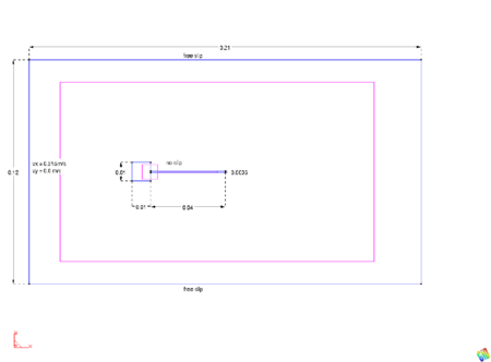
| − | An interesting validation example for the iterative solution scheme of Section 5 is that of a square bluff body followed by a flexible cantilever plate as shown in Fig. [[#img- | + | An interesting validation example for the iterative solution scheme of Section [[#5 Restrictor Flap|5]] is that of a square bluff body followed by a flexible cantilever plate as shown in Fig. [[#img-11|11]]. The prescribed distribution of velocities is shown in the same figure. The numerical setup is reproduced following <span id='citeF-8'></span>[[#cite-8|[8]]]. The fluid characteristics are <math display="inline">\rho _f = 1.18\frac{Kg}{m^3}, \mu=1.8e-5\frac{Kg}{m s} </math> the structure has a elastic modulus of <math display="inline">200000\frac{N}{m^2}</math> and a density <math display="inline">\rho _{s}=2000\frac{Kg}{m^3}</math> with the first three natural frequencies at 0.61,3.8 and 10.6 Hz. |
By applying a constant velocity at the inflow <math display="inline">U_{inflow}=0.315\frac{m}{s}</math>, the bluff body sheds Von Karman vortices with a frequency of 3.7 Hz. (on the rigid system) close to the second natural frequency of the structure. In the rigid case the pressure oscillations are relatively small. Consequently only small displacement motion is expected due to the vortex shedding. | By applying a constant velocity at the inflow <math display="inline">U_{inflow}=0.315\frac{m}{s}</math>, the bluff body sheds Von Karman vortices with a frequency of 3.7 Hz. (on the rigid system) close to the second natural frequency of the structure. In the rigid case the pressure oscillations are relatively small. Consequently only small displacement motion is expected due to the vortex shedding. | ||
| Line 1,424: | Line 1,412: | ||
Given the proximity between the shedding frequency and the structural frequency we can expect a large amplitude “resonant” motion. After a first phase of growth, the amplitude of vibration is however expected to reach a stable solution with a peak amplitude of around 0.08m. | Given the proximity between the shedding frequency and the structural frequency we can expect a large amplitude “resonant” motion. After a first phase of growth, the amplitude of vibration is however expected to reach a stable solution with a peak amplitude of around 0.08m. | ||
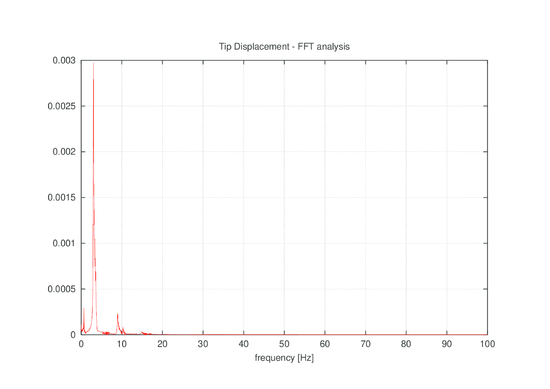
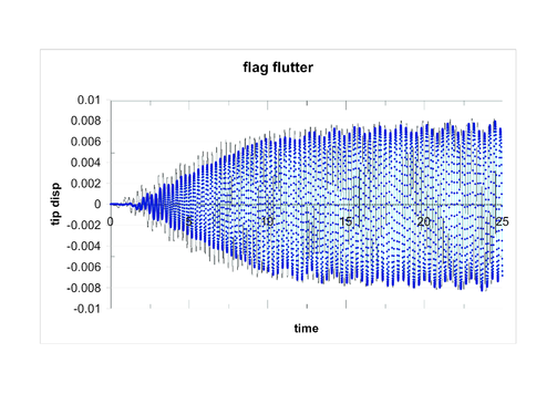
| − | Loose coupling procedures based on high order prediction steps (see <span id='citeF- | + | Loose coupling procedures based on high order prediction steps (see <span id='citeF-5'></span>[[#cite-5|[5]]]) are known to be unstable for this example. On the other hand, procedures based on a first order prediction step enforce poorly the energy conservation at the interface, leading to an important numerical positive damping (unless the time step is very small). This example was in fact originally proposed as an argument for the necessity of implicit procedures for non-linear aeroelasticity problems. The results shown were however obtained using the loosely coupled fractional step procedure described in this work. The Fourier transform of the displacement history is given in Fig. [[#img-12|12]]. The leading peak is found at a frequency of 3.04Hz in good agreement with the value of 3.1Hz published in <span id='citeF-8'></span>[[#cite-8|[8]]]. The displacement history of the tip is reported in Fig. [[#img-13|13]] on top of the history reported in <span id='citeF-9'></span>[[#cite-8|[8]]]. The excellent agreement found proves the effectiveness of our scheme for challenging simulations. |
| − | |||
| − | + | <div id='img-11'></div> | |
| − | + | ||
| − | <div id='img- | + | |
{| class="floating_imageSCP" style="text-align: center; border: 1px solid #BBB; margin: 1em auto; width: 100%;max-width: 100%;" | {| class="floating_imageSCP" style="text-align: center; border: 1px solid #BBB; margin: 1em auto; width: 100%;max-width: 100%;" | ||
|- | |- | ||
| − | |[[Image:Draft_Samper_231103336- | + | |[[Image:Draft_Samper_231103336-flag_view.png|450px|Flexible plate behind a square bluff body - view of the domain]] |
|- style="text-align: center; font-size: 75%;" | |- style="text-align: center; font-size: 75%;" | ||
| − | | colspan="1" | '''Figure | + | | colspan="1" | '''Figure 11:''' Flexible plate behind a square bluff body - view of the domain |
|} | |} | ||
| − | <div id='img- | + | <div id='img-12'></div> |
{| class="floating_imageSCP" style="text-align: center; border: 1px solid #BBB; margin: 1em auto; width: 100%;max-width: 100%;" | {| class="floating_imageSCP" style="text-align: center; border: 1px solid #BBB; margin: 1em auto; width: 100%;max-width: 100%;" | ||
|- | |- | ||
| − | |[[Image:Draft_Samper_231103336- | + | |[[Image:Draft_Samper_231103336-fftanalysis.png|550px|Flexible plate, Fourier analysis of tip displacement]] |
|- style="text-align: center; font-size: 75%;" | |- style="text-align: center; font-size: 75%;" | ||
| − | | colspan="1" | '''Figure | + | | colspan="1" | '''Figure 12:''' Flexible plate, Fourier analysis of tip displacement |
|} | |} | ||
| + | |||
| + | <div id='img-13'></div> | ||
| + | {| class="floating_imageSCP" style="text-align: center; border: 1px solid #BBB; margin: 1em auto; width: 100%;max-width: 100%;" | ||
| + | |- | ||
| + | |[[Image:Draft_Samper_231103336-tipdisp.png|503px|Flexible plate, tip displacement history - Numerical results]] | ||
| + | |- style="text-align: center; font-size: 75%;" | ||
| + | | colspan="1" | '''Figure 13:''' Flexible plate, tip displacement history - Numerical results | ||
| + | |} | ||
| + | |||
| + | ==7 Application to the aeroelastic analysis of a bridge== | ||
| + | |||
| + | We propose a third application for the simplest (and fastest) fractional step algorithm proposed in the first part of the paper. The goal of this example is twofold: from one side our interest is in showing that the algorithm actually works. Also prove that the coupling error is dominated by the fluid solution phase rather than by the coupling procedure. | ||
| + | |||
To do so we will focus our attention on the calculation of the flutter derivatives for a long span bridge deck (The Great Belt bridge section) under a constant wind speed. First we present briefly the engineering theory, then we review two methods used for the experimental determination of the coefficients needed, and finally we will show that in comparison to experimental and analytical results the fractional step procedure delivers satisfactory results. | To do so we will focus our attention on the calculation of the flutter derivatives for a long span bridge deck (The Great Belt bridge section) under a constant wind speed. First we present briefly the engineering theory, then we review two methods used for the experimental determination of the coefficients needed, and finally we will show that in comparison to experimental and analytical results the fractional step procedure delivers satisfactory results. | ||
| Line 1,475: | Line 1,473: | ||
The most frequent approach in the numerical study of the bridge aerodynamic problems is focused on the direct determination of the flutter limit <span id='citeF-19'></span><span id='citeF-20'></span><span id='citeF-21'></span><span id='citeF-22'></span>[[#cite-19|[19,20,21,22]]]. This is generally measured through the direct assesment of the system's energy, or possibly by the analysis of the displacement history. Unfortunately many factors come into play in this process making difficult the identification of the error sources. Even if in general these errors are on the numerical side it is interesting that even the experimental results may be affected by factors such as the correspondence of the numerical Reynolds to the real one, or the blockage ratio for the model tested. | The most frequent approach in the numerical study of the bridge aerodynamic problems is focused on the direct determination of the flutter limit <span id='citeF-19'></span><span id='citeF-20'></span><span id='citeF-21'></span><span id='citeF-22'></span>[[#cite-19|[19,20,21,22]]]. This is generally measured through the direct assesment of the system's energy, or possibly by the analysis of the displacement history. Unfortunately many factors come into play in this process making difficult the identification of the error sources. Even if in general these errors are on the numerical side it is interesting that even the experimental results may be affected by factors such as the correspondence of the numerical Reynolds to the real one, or the blockage ratio for the model tested. | ||
| − | In practice, at least two techniques exist for the experimental determination of the flutter derivatives. One based on the prescription of the section motion and on the analysis of the history of the forces applied from the fluid to the structure. The second one is based on the analysis of the displacement history of the section model mounted on springs. Details on the procedure used for the identification of the aeroelastic derivatives in the two cases are given in the Appendix. | + | In practice, at least two techniques exist for the experimental determination of the flutter derivatives. One based on the prescription of the section motion and on the analysis of the history of the forces applied from the fluid to the structure. The second one is based on the analysis of the displacement history of the section model mounted on springs. Details on the procedure used for the identification of the aeroelastic derivatives in the two cases are given in the [[#Appendix. Computation of aeroelastic derivatives for bridge analysis|Appendix]]. |
Both of those experimental procedures can be reproduced numerically. The forced vibration approach does not involve any coupling error and can be considered as a reference solution for evaluating the equivalent coupled approach. Its performance is governed exclusively by the properties of the fluid solver and by the mesh used for the computation. | Both of those experimental procedures can be reproduced numerically. The forced vibration approach does not involve any coupling error and can be considered as a reference solution for evaluating the equivalent coupled approach. Its performance is governed exclusively by the properties of the fluid solver and by the mesh used for the computation. | ||
| Line 1,483: | Line 1,481: | ||
A similar result could be achieved by direct comparison with the experimental results once the ability of the fluid solver to describe correctly the phenomena is guaranteed. This would require fine meshes greatly increasing the computational cost, thus making the testing procedure unsuitable for the study of different coupling strategies. On the other hand by comparing two numerical results obtained under the same condition we can directly asses the impact of the coupling on the final results, which is the objective of current work. | A similar result could be achieved by direct comparison with the experimental results once the ability of the fluid solver to describe correctly the phenomena is guaranteed. This would require fine meshes greatly increasing the computational cost, thus making the testing procedure unsuitable for the study of different coupling strategies. On the other hand by comparing two numerical results obtained under the same condition we can directly asses the impact of the coupling on the final results, which is the objective of current work. | ||
| + | ===7.1 Numerical setup=== | ||
| − | + | The identification techniques described above were used for the identification of the aeroelastic derivatives of a bridge cross-section. Due to the availability of validation data the cross-section of the great belt suspension span in Denmark was chosen for the benchmark exercise. This section, was studied numerically and experimentally <span id='citeF-20'></span><span id='citeF-23'></span><span id='citeF-24'></span>[[#cite-20|[20,23,24]]]. The experimental plots used for the comparison were taken from <span id='citeF-25'></span>[[#cite-25|[25]]]. The validation procedure is described as below. | |
| − | + | ||
| − | + | ||
| − | | | + | |
| + | Description of the validation procedure: | ||
* Construct the model and compute a starting solution by keeping the section fixed | * Construct the model and compute a starting solution by keeping the section fixed | ||
* Prescribe the motion of the section and identify the aeroelastic derivatives for different frequences | * Prescribe the motion of the section and identify the aeroelastic derivatives for different frequences | ||
| Line 1,494: | Line 1,491: | ||
* Calculate the aeroelastic derivatives in free motion | * Calculate the aeroelastic derivatives in free motion | ||
* Evaluate the coupling properties by comparing the two curves | * Evaluate the coupling properties by comparing the two curves | ||
| − | + | <br /> | |
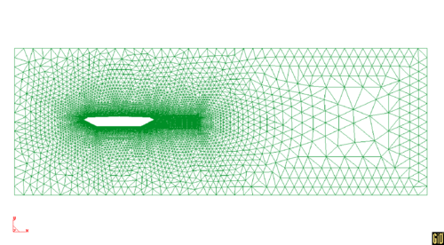
| − | + | The analysis domain, as represented in Fig.[[#img-14|14]], was chosen so to keep around 6% the ratio between the section chord and the vertical dimension of the domain in order to minimize the blockage effect. An unstructured mesh composed of 9197 nodes and 17862 triangular three-noded elements with a minimum element size (around the bridge deck) of 0.15m was used. | |
| − | + | <div id='img-14'></div> | |
| + | {| class="floating_imageSCP" style="text-align: center; border: 1px solid #BBB; margin: 1em auto; width: 100%;max-width: 100%;" | ||
| + | |- | ||
| + | |[[Image:Draft_Samper_231103336-mesh_picture.png|500px|Cross section of Great Belt suspension bridge.]] | ||
| + | |- style="text-align: center; font-size: 75%;" | ||
| + | | colspan="1" | '''Figure 14:''' Cross section of Great Belt suspension bridge. | ||
| + | |} | ||
| − | + | <div class="center" style="font-size: 75%;"> | |
| + | '''Notes:''' View of the mesh used in the computations. | ||
| + | </div> | ||
Only pressure forces are transferred to the structure, negleting the contribution of viscous forces (which would be poorly approximated by a mesh as the one described). This approximation is commonly accepted for bridges which behave as bluff bodies. | Only pressure forces are transferred to the structure, negleting the contribution of viscous forces (which would be poorly approximated by a mesh as the one described). This approximation is commonly accepted for bridges which behave as bluff bodies. | ||
| − | The actual dimensions of the cross-section were used with a Reynolds number that was consequently far greater than the one reproduced in wind tunnel testing. Even if this could theoretically lead to important discrepancies with the experimental data, it is currently believed that for the case of interest the derivatives are fairly independent of the Reynolds number of the flow. The inflow velocity was therefore taken as 10m/s corresponding to a <math display="inline">(Re = \frac{v_{\infty }B}{\nu }\approx 2 | + | The actual dimensions of the cross-section were used with a Reynolds number that was consequently far greater than the one reproduced in wind tunnel testing. Even if this could theoretically lead to important discrepancies with the experimental data, it is currently believed that for the case of interest the derivatives are fairly independent of the Reynolds number of the flow. The inflow velocity was therefore taken as 10m/s corresponding to a <math display="inline">(Re = \frac{v_{\infty }B}{\nu }\approx 2\times 10^7</math>). |
No turbulence model was included in the simulation however a subgrid scale stabilization method was used []. | No turbulence model was included in the simulation however a subgrid scale stabilization method was used []. | ||
| − | + | The structural displacements were kept small with a maximum pitching angle of 3deg and a maximum motion in heave of 1.57m in accordance to the values reported in <span id='citeF-24'></span><span id='citeF-17'></span>[[#cite-24|[24]], [[#cite-17|17]]]. The reduced frequency <math display="inline">\frac{U_{inflow}}{nB}</math>, was varied by changing the value of the frequency <math display="inline">n</math> of the prescribed sectional motion. This allowed to start all the simulations exactly from the same initial conditions. An initial velocity was prescribed to the structure in order to study the decay or growth of the initial solution. This velocity was chosen so to provide a maximum displacement “in vacuo” corresponding to the one for the prescribed motion setting. This was enforced by considering that in absence of fluid the system is conservative, from which follows | |
| − | + | ||
| − | + | ||
| − | + | ||
| − | + | ||
| − | + | ||
| − | + | ||
| − | + | ||
| − | The structural displacements were kept small with a maximum pitching angle of 3deg and a maximum motion in heave of 1.57m in accordance to the values reported in <span id='citeF-24'></span><span id='citeF-17'></span>[[#cite-24|[24,17]]]. The reduced frequency <math display="inline">\frac{U_{inflow}}{nB}</math>, was varied by changing the value of the frequency <math display="inline">n</math> of the prescribed sectional motion. This allowed to start all the simulations exactly from the same initial conditions. An initial velocity was prescribed to the structure in order to study the decay or growth of the initial solution. This velocity was chosen so to provide a maximum displacement “in vacuo” corresponding to the one for the prescribed motion setting. This was enforced by considering that in absence of fluid the system is conservative, from which follows | + | |
{| class="formulaSCP" style="width: 100%; text-align: left;" | {| class="formulaSCP" style="width: 100%; text-align: left;" | ||
| Line 1,528: | Line 1,525: | ||
|} | |} | ||
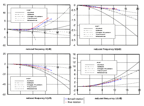
| − | This setup was used for the assessment of the partitioned coupling procedures implemented in Kratos, a Multi-Physics code developed at | + | This setup was used for the assessment of the partitioned coupling procedures implemented in Kratos, a Multi-Physics code developed at [http://www.cimne.com/kratos CIMNE]. Both first and second order solvers were used, the latter being vastly superior in reproducing the experimental curves. For the first order case, showed in Fig. [[#img-15|15]] the mesh and step size are not sufficiently fine to reproduce the experimental curves. The results of interest are however clearly met as the identified derivatives follow a similar behavior using both identification techniques, proving that the error is governed by the fluid solution and not by the coupling error. This allows in practice to use a much coarser mesh than that normally be needed to eliminate the errors in the fluid solution, which in turn provides an advantage for the quick assessment of the performance of the coupling procedure. |
| + | |||
| + | <div id='img-15'></div> | ||
| + | {| class="floating_imageSCP" style="text-align: center; border: 1px solid #BBB; margin: 1em auto; width: 100%;max-width: 100%;" | ||
| + | |- | ||
| + | |[[Image:Draft_Samper_231103336-A2_A3_H2_H3.png|550px|Fitting of experimental aeroelastic derivatives, using a first order accurate solver for the fluid domain]] | ||
| + | |- style="text-align: center; font-size: 75%;" | ||
| + | | colspan="1" | '''Figure 15:''' Fitting of experimental aeroelastic derivatives, using a first order accurate solver for the fluid domain | ||
| + | |} | ||
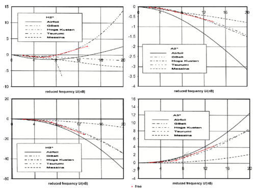
We remark that the use of a second order solver for the fluid solution (on the same computational setup) reproduces accurately the experimental curves using the free vibration procedure (see Fig. [[#img-16|16]]). This confirms the good performance of the coupling procedure used. | We remark that the use of a second order solver for the fluid solution (on the same computational setup) reproduces accurately the experimental curves using the free vibration procedure (see Fig. [[#img-16|16]]). This confirms the good performance of the coupling procedure used. | ||
| + | |||
| + | <div id='img-16'></div> | ||
| + | {| class="floating_imageSCP" style="text-align: center; border: 1px solid #BBB; margin: 1em auto; width: 100%;max-width: 100%;" | ||
| + | |- | ||
| + | |[[Image:Draft_Samper_231103336-a2_a3_h2_h3_2nd.png|500px|Free rotation fitting of experimental aeroelastic derivatives using a second order accurate solver for the fluid domain]] | ||
| + | |- style="text-align: center; font-size: 75%;" | ||
| + | | colspan="1" | '''Figure 16:''' Free rotation fitting of experimental aeroelastic derivatives using a second order accurate solver for the fluid domain | ||
| + | |} | ||
==8 Conclusions== | ==8 Conclusions== | ||
| Line 1,617: | Line 1,630: | ||
[[#citeF-25|[25]]] D. Cobo del Arco and A.C. Aparicio Bengoechea. (1999) An Analysis of Wind Stability.Improvements to the Response of Suspension Bridges. CIMNE | [[#citeF-25|[25]]] D. Cobo del Arco and A.C. Aparicio Bengoechea. (1999) An Analysis of Wind Stability.Improvements to the Response of Suspension Bridges. CIMNE | ||
| − | ==Appendix | + | ==Appendix. Computation of aeroelastic derivatives for bridge analysis== |
| − | === | + | ===Forced motion procedure=== |
One first approach is based on the application of a prescribed sinusoidal motion to the bridge section which is then subjected to the fluid flow. A description of the testing procedure can be found in <span id='citeF-23'></span>[[#cite-23|[23]]] or, with a similar approach in <span id='citeF-21'></span>[[#cite-21|[21]]]. The “experimental” setup can be expressed as follows: | One first approach is based on the application of a prescribed sinusoidal motion to the bridge section which is then subjected to the fluid flow. A description of the testing procedure can be found in <span id='citeF-23'></span>[[#cite-23|[23]]] or, with a similar approach in <span id='citeF-21'></span>[[#cite-21|[21]]]. The “experimental” setup can be expressed as follows: | ||
| − | * | + | * Fix the horizontal and vertical motion of the cross section |
| − | * | + | * Prescribe a sinusoidal pitching motion (a prescribed rotation) with a known angular frequency |
| − | * | + | * Measure the forces and moments on the section |
| − | * | + | * Perform a (linear) least-square fitting of the measured forces with an equation in the form <math display="inline">x(t) = Asin(\omega t + \phi )</math> both for the moment history and lift history. |
| − | * | + | * Use the fitted values for <math display="inline">A </math> and <math display="inline"> \phi </math> to identify the coefficients as described below |
The identification is performed through a (linear) least square fit of the recorded moment and lift histories using an expression of the form <math display="inline">Asin(\omega t + \phi )</math>. The simple trigonometric identity | The identification is performed through a (linear) least square fit of the recorded moment and lift histories using an expression of the form <math display="inline">Asin(\omega t + \phi )</math>. The simple trigonometric identity | ||
| Line 1,641: | Line 1,654: | ||
|} | |} | ||
| − | together with the auxiliary vectors (N is the number of measured time steps, <math display="inline">\delta t</math> the stepsize) | + | together with the auxiliary vectors (<math>N</math> is the number of measured time steps, <math display="inline">\delta t</math> the stepsize) |
{| class="formulaSCP" style="width: 100%; text-align: left;" | {| class="formulaSCP" style="width: 100%; text-align: left;" | ||
| Line 1,771: | Line 1,784: | ||
| − | {| class="floating_tableSCP" style="text-align: | + | {| class="floating_tableSCP wikitable" style="text-align: center; margin: 1em auto;min-width:50%;" |
| − | |+ style="font-size: 75%;" |<span id='table- | + | |+ style="font-size: 75%;" |<span id='table-A1'></span>'''Table. A1''' Relations for computing the aeroelastic derivatives: the upper index indicates the prescribed sectional motion, the lower index the equation used in fitting the load history |
|- | |- | ||
| − | | | + | |style="text-align: center;" |Prescribed heave: |
| − | + | ||
| − | + | ||
| − | + | ||
| − | | | + | |
| − | + | ||
| − | + | ||
|- | |- | ||
| style="text-align: center;" | <math> H_4 = {\frac{{ B^{heave}_{lift}}}{\rho \,{B}^{2}{w}^{2}{ y_0}}} \, ; \, H_1 = {\frac{{ C^{heave}_{lift}}}{\rho \,{B}^{2}{w}^{2}{ y_0}}} </math> | | style="text-align: center;" | <math> H_4 = {\frac{{ B^{heave}_{lift}}}{\rho \,{B}^{2}{w}^{2}{ y_0}}} \, ; \, H_1 = {\frac{{ C^{heave}_{lift}}}{\rho \,{B}^{2}{w}^{2}{ y_0}}} </math> | ||
| − | |||
| − | |||
| − | |||
| − | |||
| − | |||
| − | |||
| − | |||
|- | |- | ||
| style="text-align: center;" | <math> A_4 = {\frac{{ B^{heave}_{mom}}}{\rho \,{B}^{3}{w}^{2}{ y_0}}} \, ; \, A_1 = {\frac{{ C^{heave}_{mom}}}{\rho \,{B}^{3}{w}^{2}{ y_0}}} </math> | | style="text-align: center;" | <math> A_4 = {\frac{{ B^{heave}_{mom}}}{\rho \,{B}^{3}{w}^{2}{ y_0}}} \, ; \, A_1 = {\frac{{ C^{heave}_{mom}}}{\rho \,{B}^{3}{w}^{2}{ y_0}}} </math> | ||
| − | |||
| − | |||
| − | |||
| − | |||
| − | |||
|- | |- | ||
| − | + | |style="text-align: center;" |Prescribed rotation: | |
| − | + | ||
|- | |- | ||
| style="text-align: center;" | <math> H_3 = {\frac{{ B^{pitch}_{lift}}}{\rho \,{B}^{3}{w}^{2}{ \alpha _0}}} \, ; \, H_2 = {\frac{{ C^{pitch}_{lift}}}{\rho \,{B}^{3}{w}^{2}{ \alpha _0}}} </math> | | style="text-align: center;" | <math> H_3 = {\frac{{ B^{pitch}_{lift}}}{\rho \,{B}^{3}{w}^{2}{ \alpha _0}}} \, ; \, H_2 = {\frac{{ C^{pitch}_{lift}}}{\rho \,{B}^{3}{w}^{2}{ \alpha _0}}} </math> | ||
| − | |||
| − | |||
| − | |||
| − | |||
| − | |||
| − | |||
| − | |||
|- | |- | ||
| style="text-align: center;" | <math> A_3 = {\frac{{ B^{pitch}_{mom}}}{\rho \,{B}^{4}{w}^{2}{ \alpha _0}}} \, ; \, A_2 = {\frac{{ C^{pitch}_{mom}}}{\rho \,{B}^{4}{w}^{2}{ \alpha _0}}} </math> | | style="text-align: center;" | <math> A_3 = {\frac{{ B^{pitch}_{mom}}}{\rho \,{B}^{4}{w}^{2}{ \alpha _0}}} \, ; \, A_2 = {\frac{{ C^{pitch}_{mom}}}{\rho \,{B}^{4}{w}^{2}{ \alpha _0}}} </math> | ||
| − | |||
| − | |||
|} | |} | ||
| − | which represents a heaving motion, it is possible to identify the remaining four derivatives. Table ([[#table- | + | which represents a heaving motion, it is possible to identify the remaining four derivatives. Table ([[#table-A1|A1]]) summarizes the relevant formulae for computing the aeroelastic derivatives. |
| − | === | + | ===Free vibration method=== |
| − | The second procedure for the determination of the aeroelastic coefficients is based on the analysis of the displacement history of the sectional model mounted on a set of springs of known stiffness. This testing procedure is more challenging for the interaction as it involves a completely coupled analysis, which introduces a further error source. An excellent example of application to bridges can be found in | + | The second procedure for the determination of the aeroelastic coefficients is based on the analysis of the displacement history of the sectional model mounted on a set of springs of known stiffness. This testing procedure is more challenging for the interaction as it involves a completely coupled analysis, which introduces a further error source. An excellent example of application to bridges can be found in <span id='citeF-19'></span><span id='citeF-22'></span>[[#cite-19|[19]]], [[#cite-22|[22]]]. In these works however the free vibration procedure is used to assess directly the flutter speed by evaluating the energy variation. |
The original identification procedure as proposed by Scanlan <span id='citeF-17'></span>[[#cite-17|[17]]], is based on a three step analysis in which the cross section mounted on springs is first restrained in heave, then in rotation and finally left completely free. This was needed as the available setup allowed to record exclusively the displacement history but not the restrain forces. The approach described in the following is slightly different and it involves only two sets of simulations by making use of both displacement histories and forces records. | The original identification procedure as proposed by Scanlan <span id='citeF-17'></span>[[#cite-17|[17]]], is based on a three step analysis in which the cross section mounted on springs is first restrained in heave, then in rotation and finally left completely free. This was needed as the available setup allowed to record exclusively the displacement history but not the restrain forces. The approach described in the following is slightly different and it involves only two sets of simulations by making use of both displacement histories and forces records. | ||
| Line 1,951: | Line 1,936: | ||
which is the desired result. | which is the desired result. | ||
| − | === | + | ===Free heave=== |
The identification of the remaining four derivatives follows a similar path. Once the non linear fitting of the lift equation is performed, two of the aeroelastic parameters can be identified as | The identification of the remaining four derivatives follows a similar path. Once the non linear fitting of the lift equation is performed, two of the aeroelastic parameters can be identified as | ||
| Line 1,977: | Line 1,962: | ||
|} | |} | ||
| − | The identification of the parameters can be performed by non linear fitting techniques. The nonlinear fitting routines provided in scipy a scientific library included in | + | The identification of the parameters can be performed by non linear fitting techniques. The nonlinear fitting routines provided in scipy a scientific library included in [http://www.python.org python] were used in the computations. The convergence of the fitting process was ensured by taking as initial value for the fitting process an estimate for all the relevant parameters. |
Latest revision as of 14:25, 9 January 2019
Published in Engineering Computations Vol. 27 (1), pp. 20-56, 2010
doi: 10.1108/02644401011008513
Abstract
The field of fluid-structure interaction (FSI) has important applications ranging from the bio-medical to the civil and aeronautical engineering fields. Despite the different approaches developed over recent years the general solution of FSI problems remains however far from being closed. This paper addresses the theoretical analysis of a several partitioned solution schemes for FSI. This is achieved by choosing a simple but representative model problem which allows to obtain analytical results. A loose coupling partitioned procedure is presented first. An iterative version of the same algorithm is presented next together with an analysis of its convergence properties and a brief discussion of a possible acceleration strategy. Finally a new iterative strategy based on solving a modified equation is described. Some examples of application of the partitioned algorithms considered are presented including the aeroelastic analysis of a bridge.
Keywords: Fluids, Structures, Flow, Fluid dynamics, Programming and algorithm theory, Iterative methods
1 Introduction
The coupling between different physical phenomena constitute a challenge in many applications of practical interest. Empirical or analytical techniques which classically provide a satisfactory description of coupled problems at the asymptotic limits, do not guarantee the necessary guidance when the coupling becomes strong. The field of FSI (fluid-structure interaction) represents an important and active area of research due its relevance in many problems in science and engineering.
Until recent times the numerical simulation of strongly coupled FSI problems was considered to be unviable. Experimental wind-tunnel testing were for long the only approach for the design of complex aeroelastic interaction-sensitive structures such as bridge decks or slender towers. Although well established, wind tunnel testing is often expensive and time-consuming. In addition some concerns on the quality of the predictions arise when severe scale reduction is needed to fit the model in the test facility.
The maturity of numerical finite element (FE) techniques in the fields of computational fluid dynamics (CFD) and structural dynamics, together with the increasing computational power start nowadays to make competitive the purely numerical approach for solving FSI problems.
From a mathematical point a wide class of coupled problems can be represented symbolically as
|
where and are functions that denote the behaviour of the two coupled systems and represent some significative variables for each of the systems. Typically subscripts and denote structure and fluid contributions, respectively. Eqns.(1) and (2) can be linearized to give a system in the form
|
|
(3) |
where the off-diagonal terms of the tangent (or Jacobian) stiffness matrix express the dependency of one field on the variations of the second. This form guarantees theoretically optimal quadratic convergence properties. In practice the two symbolic operators and are non linear and in most cases are not explicitly known. Hence the computation of the derivatives in Eqn(3) may be difficult or undesiderable for other reasons.
Even if theoretically possible, the linearization of the fluid field is usually not performed, as it is often preferred to rely on fixed point type iterations to solve the non linearities. This implies that the computation of the jacobian in Eqn(3) would involve a redefinition of the fluid strategy which is not desiderable from the point of view of software modularity. This makes full Newton schemes generally unattractive for solving FSI problems. Further the resulting “monolithic” matrix, would inherit the same conditioning problems from the corresponding fluid counterpart. Thus making its inversion difficult using any iterative technique.
Two main approaches exist for solving this impasse. The purely algebraic one focuses on the iterative solution of Eqns(1) and (2) approaching as much as possible the optimal behavior of the Newton system in Eqn(3). The second one focuses on partitioned (sometimes called “explicit”) coupling techniques where convergence to the coupled solution is guaranteed by a careful adjustment of the predicted variable and of the data transferred between the interacting domains.
The first approach has its simpler expression in the so called Block-Jacobi or Block-Seidel iterations which involve the following steps
The above scheme can be eventually modified to include a relaxation step such as . This technique is very effective for some problems. Nevertheless in some cases may not be computationally competitive versus the partitioned technique. The choice of the optimal relaxation factor is still matter of research. For instance in [1], [2] the Aitken accelerator is used to improve the convergence of the scheme. Alternatively a number of quasi-Newton techniques were presented over the years in an effort for achieving quadratic convergence when solving Eqn(3). An interesting description can be found in [3], [4] where iterative solvers are exploited for solving the coupled problem without building explicitly the Jacobian matrix.
This matrix-free approach is optimal from the point of view of software modularity, and naturally tends to the solution of the monolithic formulation from which it inherits stability properties. The disadvantage is the high computational cost due to the need for solving the implicit system to a high degree of accuracy.
In addition, the partitioned approach relies on a careful design of the prediction and correction phases in order to minimize the spurious energy introduced in the system. Pioneering work on the subject was reported by [5] who developed partitioned solution strategies for large scale parallel computing applications in aeronautics [6].
Given the absence of a common mathematical formulation for the two coupled fields the investigation of the stability properties of the different methods is extremely challenging. A 1D case is investigated in [6] (for a compressible flow) while in [5] a simple test is advocated to assess the stability of a partitioned scheme. Even if the proposed method has no general mathematical validity it was shown to discriminate successfully stable methods from unstable ones. The techniques proposed were tested on large aeronautical examples [7] and provided satisfactory results in describing experimental flutter envelopes on real aircrafts. They are also believed to be effective in dealing with linear and non-linear problems as long as the displacements are small. Some concern arises however regarding their robustness in dealing with FSI problems for highly flexible structures and a truly incompressible fluid. Recent results however have proven their applicability to general cases when using compressible flow solvers.
The application of space-time FE based approaches can be found in [8] and [9] with reference to both civil and aeronautical applications. Finally some examples of applications to large flexible civil engineering structures can be found in [10],[11].
The objective of this work is to discuss several algorithms for solving coupled problems of the type of Eqn(2) by considering a loose coupling partitioned approach and two possible improvements by iteration. The effort is to provide a framework to study the properties of the coupling procedures by evaluating the impact of different time integration schemes. The layout of the paper is the following. First a simple but representative 1D model problem is chosen. A partitioned solution strategy is identified and applied symbolically to the model problem. This allows us to obtaining an error matrix which depends on the time integration scheme chosen. Two possibilities of iterative improvement of the partitioned method is discussed and an estimate of the error evolution with the iterations is given. Finally an enhanced iterative strategy based on the solution of a modified equation is described. The partitioned schemes studied are applied to a number of FSI problems including to the solution of a real problem in bridge aerodynamics for which wind tunnel results are available for comparisons.
2 The Model Problem
Partitioned (or staggered) techniques are appealing for solving coupled FSI problems as they allow the use of state-of-the-art single-field solvers. As such they are widely used in many fields of application. The disadvantage is often connected to a lack of robustness in dealing with some category of FSI problems, typically involving truly incompressible fluids or requiring long-term analyses. Strong or fully coupling techniques on the other hand guarantee a convergence to the monolithic solution by providing a completely “implicit” coupling between the different fields. In practice however, they tend to be costly and may experience convergence difficulties when dealing with complex problems.
The aim of the paper is to investigate the reasons behind this difficulties. The same effort was attempted in different works, see for example [5] for a discussion of partitioned methods or [12] for an analysis of a semi-implicit technique. Both papers present interesting results and define satisfactory algorithms for many applications.
This work follows a slightly different path by considering a further requirement: an ideal coupling scheme should be robust upon changes in the single-field solvers. In other words, its properties should be independent from the particular solver chosen for each of the coupling fields. As a consequence, the particular features of the solvers should not be exploited in discussing a coupling algorithm, unless the interest focuses exclusively on a very particular choice. In order to highlight our approach a simple linearized model problem is chosen and the coupling algorithm proposed is applied to its solution.
The choice for such a simple model problem is unfortunately non univocal in FSI, and needs to be justified. To do so we assume that in the “common” engineering practice the fluid solution is often avoided and the interaction between a structure and the surrounding fluid is often described by the exchange of a pressure force between the fluid and the structure [13]. Such pressure force is often modeled as
|
|
(4) |
where coefficients and generally depend on the frequency of the motion. A careful choice of such constants for aeroelastic analysis (generally from a good fit to wind tunnel data) can lead to an excellent description of the most relevant features of the wind action on a structure. This implies that this simple model can reproduce correctly the coupling between the structure and the fluid.
A load defined by Eqn(4), which is naturally suited for the frequency domain analysis, generally needs to be transformed in the time domain. Such transformation is not trivial (see for example [14]) and will not be discussed here. The interesting result is that Eqn(4) can be substituted in the time domain by a relation of the type
|
|
(5) |
eventually generalized including history dependent terms. In Eqn(5) index denotes terms in the fluid domain computed at the fluid-structure interface. This implies that the instantaneous force exerted by the fluid on the structure, depends directly on the acceleration, velocity and displacement of the structure itself. The dependence on the acceleration in particular is crucial and the corresponding “mass-like” term is known as “added mass”.
Interestingly enough a similar dependence of the interaction forces on the structural motion can be obtained from the analysis of the continuum problem [12] or from a simple algebraic manipulation of the discrete Navier Stokes problem. The important point is that a simple model as that of Eqn(5) captures satisfactorily the important features of the coupling, and is thus appropriate to define a test problem.
The idea we will exploit here is conceptually simple: let us consider a 1D problem representing the interaction between a given structure and the surrounding fluid. Without loss of generality we can assume that the abstract problem defined by Eqns(1) and (2) can be rewritten as:
|
where indices and denote terms emanating from the solid and fluid domains computed at the fluid-structure interface, is the pressure force that originates from the coupling and it plays the role of the “coupling variable” in the study of the interaction. Eqns(6) and (7) represent the simplest abstract form of the coupled equations for a FSI problem. The performance of a given coupling algorithm can be therefore assessed by applying it to the solution of Eqns(6) and (7).
It is intuitive that procedures that “behave well” on a test problem with the form of Eqn(6) and (7) for any physically relevant choice of the problem parameters can describe correctly the effect of the fluid on the structure. In other words procedures that solve accurately the test problem can be expected to be well suited for the simulation of the FSI interaction for cases where a model giving the pressure force by an expression of the form of Eqns(4) is acceptable for design purposes.
Clearly the time discretization of Eqns(6) and (7) implicitly contains an error connected to the choice for the time integration algorithm. This error has little interest as it does not depend on the way we enforce the coupling. Our interest is rather connected to the error between the approximate and exact discrete solutions of the coupling problem. In other words we assume that no error cancelation manifests due to the interaction of the different solution schemes. Note that this is a strong assumption. Different approaches, in particular the work of Farhat and Piperno [5] , exploit exactly the error cancelation to tune the features of their coupled solvers. Not considering the error cancelation is however mandatory if the requirement of “independence from the single-field solvers” needs to be enforced.
As a final comment we point out that necessary features for a “good” coupled time integrator are (Felippa [15])
- preserve the stability of stable mathematical models
- manifest the instability of unstable mathematical models.
Effort will be devoted in this work to studying the stability properties of the coupling algorithms analysed.
2.1 A simple form for the analysis of the discrete coupling problem
The system described by Eqn(6) and (7) can be rewritten as a reduced monolithic problem simply by substituting the second equation into the first. To simplify the subsequent developments we will express the mass and stiffness coefficient for the fluid ( and ) as a ratio to the correspondent structural quantities. This gives
|
where the structural mass () is assumed to have a unit value without loss of generality.
Substituting the value of in Eqn(7) into Eqn(6) and using Eqns(8)–(10) yields the monolithic system
|
|
(11.a) |
or
|
|
(11.b) |
Eqn(11.b) or (11.a) are equivalent to Eqns(6) and (7) and express synthetically the dynamic behaviour of the coupled problem. We are mostly interested in the case where the presence of the fluid influence the transient behaviour of the structure. We shall however assume that even in presence of a very important coupling the mathematical behaviour of the coupled system is preserved, or, in other words that the overall mass and stiffness are both non negative. Note however that a negative damping (leading to a divergent structural behaviour) can be considered. These considerations allows us to assume that
|
|
(12) |
|
|
(13) |
In general we can expect the coupled system to be heavier than the single system, which suggests that the stricter condition will hold.
Up to this point no approximation was introduced and Eqn(11.a) or (11.b) is still completely equivalent to the system described in Eqns(6) and (7). To proceed further we perform the discretization in time. Without loss of generality we shall consider that a general class of time integrators can be expressed symbolically as
| (14)
| where the choice of the linear operators , and defines the time integrator used and the effect of external forces. Such general form allows us to predict the evolution of a system between the time stations and when subjected to a force varying linearly between the values and . By defining the auxiliary vectors
we express the model problem of Eqn(11.b) in the simple matrix form
and the “pressure force” (the term exchanged between the first and second equation in Eqns(6) and (7)) at the initial and final time stations as
This suffices to express in matrix form both the exact solution and the approximate one. 2.2 Discrete solution of the exact coupling problemThe evaluation of the exact coupled solution can be performed preserving the matrix notation introduced in the previous section. To do so it is necessary to express the link between the pressure and the structural motion. Dynamic equilibrium (Eqn(6)) gives
substituting back into Eqn(17) and using the definitions in Eqns(8)–(10), we recover the relation
On the other hand the structure is advanced in time following the time integration rule of Eqn(14). Substituting Eqn(19) into Eqn(14) and collecting terms we obtain
which allows us to write synthetically
where
and
Eqn(21) yields the amplification form of the exact solution for the coupled problem. 2.3 A fractional step-like algorithmIn the previous section we expressed the exact solution in an amplification form, relating pressures, velocities and displacements at two consecutive time steps. Unfortunately in real life not all the information needed is available at the same time. Therefore an approximate coupling strategy needs to be devised. In this section we propose and analyse a fractional step-like partitioned approach including the following steps: Predictive step:
Correction step:
This simple strategy can be improved by successive corrections leading to the definition of an iterative strategy which minimizes the coupling error inside each time step. For such a strategy our interest focuses on the convergence properties of the iteration sequence. In the following lines we detail the prediction and correction phases. Prediction step. The pressure acting on the structure is calculated as
Then we advance in time the solution for the structure under the predicted pressure. Taking into account the form assumed for the structural integrator we obtain
grouping the two equations we get
By introducing the auxiliary matrices
with
we can express the prediction for the fluid and structural variables as
Correction step. The first step of the correction step is the computation of the corrected pressure field. To include this in our simplified model we need to calculate the predicted accelerations. Dynamic equilibrium (Eqn(18) gives
Using the definitions in Eqn(8) the corrected pressure value in the fluid can be expressed as
The final correction step for the structure has the usual form
Eqns(31 and 32) can be grouped in an amplification form as
where
Note that matrix is empty and was included only for generalization purposes. Substituting Eqn(29) into Eqn(33) we obtain
which allows us to obtain the final amplification form for the fractional step procedure as
This form will be used to study the accuracy and stability of the proposed scheme in the next sections. 2.4 Analysis of the truncation errorAssuming that the exact solution is known in steps 1 to , the truncation error of the fractional step algorithm explained in the previous section can be obtained by difference between the approximate and exact solutions. The amplification form obtained in the previous section Eqn(38) allows us the evaluation of this error. To perform this operation we observe that and can not be prescribed independently as the exact solution is used as a starting point. Typically only the displacements and velocities are prescribed and the pressure is calculated subsequently. A dynamic equilibrium relation necessarily holds relating pressures displacements and velocities in the initial steps. The definition of implies
The definition of the exact amplification matrix Eqn(22) on the other hand gives
This together with Eqn(39) allows us to express the exact solution at step in the form
Following the same rationale, the approximate solution at the given step becomes
By subtracting Eqns(41) and (42) it is possible to define a “reduced” rectangular error matrix relating the pressure and the structural variables at step with the structural variables at the former step, i.e.
with
This last equation contains all the information needed concerning the order of accuracy. The fact that is not square indicates that for the exact solution only the structural variables can be prescribed, as pressure can be calculated as a dependent variable. 2.5 Newmark and exact time integrationThe results up to this point are still general and hold for any time integration scheme with the form of Eqn(14). This allowed us to describe “symbolically” an approximate fractional-step coupling procedure and to evaluate an expression for the truncation error matrix. In the following we will consider the “exact” time integrator and the Newmark time integrator and evaluate the behaviour of the error for the two cases. We highlight that the so called “exact” integrator should guarantee exact results once the initial conditions and the values of the force at the beginning and end of the step are provided. Applying the exact time integrator within an approximate solution procedure does not guarantee an exact result. The interesting conclusion is that the coupling error obtained with both the Newmark and the exact schemes is very similar and depends on the coupling procedure rather than on the time integration procedure. The amplification matrix and the force vectors and for the Newmark time integration scheme are widely known [16]. In the most general case they take the form
with
and
where represents the time step size. We will consider in the following exclusively the second order accurate, non dissipative case. By assuming that the forces vary linearly within the time step, it is possible to work out a similar result corresponding to the exact time integrator. The amplification matrix becomes now
and the force vectors are
Substituting above expressions into Eqn(44) is straight-forward but implies some heavy algebraic calculations. Performing this operation in Maple or a similar Computer Algebra System (CAS) program presents no particular difficulty even for the general case. It is interesting to focus on the undamped case (no structural damping) as this leads to simpler results. We note that the estimates obtained hold as well for the general damped case An important (although not unexpected) result is that consistency requires the condition for the “free” parameters in the prediction step ( Eqn(24) ). The two choices and are appealing and correspond to first and second order accuracy for the predicted force, respectively. The order of this initial prediction determines that for the overall approximate time integration scheme for the coupled problem. Table 1 contains the first non-zero terms for the Taylor expansion of the error matrix. The analysis of these results shows how the same error estimates hold for the Newmark and exact time integration schemes. This feature is desiderable as it suggests that different choices for the time integration scheme can be taken without affecting the coupling error. The properties of the coupled fractional step depend however on the values assumed by the aeroelastic mass and the damping term. For or the mathematical structure of the problem changes as the overall coupled problem assumes a negative mass matrix. By assuming or (see remark 12 and 13) we obtain the inequalities
which give some insight on the damping properties of the proposed fractional step procedure.
It is of interest that these estimates hold for the general case. When the aeroelastic mass is negligible the performance of the fractional step procedure is enhanced and the overall order of accuracy is three. Using the exact time integrator we obtain the error matrix
2.6 Stability issuesTo complete the discussion we study the stability of the scheme proposed. Let us consider for simplicity the one-step (first order) fractional step scheme ( in Eqn(24)). We already know that the exact solution of the coupled problem (including both the pressure and the structural variables) can be written as
while the approximate solution, obtained via some coupling procedure, can be expressed as
where we have introduced a new error matrix relating the structural variables and the pressure. Some confusion might arise concerning the amplification matrices used. are here matrices and should not be confused with the “reduced” forms (rectangular) used for assessing the accuracy (see Table 1). A classical discussion of stability is not trivial due to the complexity of the approximate amplification matrix. We know however that stability is governed by the spectral radius of the amplification matrix. For the one-step fractional step procedure, the eigenvalues can be computed analytically. For the general case the results are very lengthy and difficult to handle. Some useful information can however be obtained by expressing the eigenvalues as functions of the auxiliary variable which is a non dimensional measure of the number of steps for integrating of one structural period. By expanding in Taylor series the expressions obtained for the eigenvalues , the leading terms of these series (which represent the results for the time step size tending to zero) give:
where the index represents the eigenvalue number. A necessary requirement for stability is that at the limit for tending to zero, the spectral radius is lower or equal to one. By taking the limit in the simplified expressions we obtain
which suggests that stability is problem dependent and the proposed procedure is unconditionally unstable for . This definition of stability is however not completely appropriate for the coupling problem of interest. For the FSI coupling both divergent and convergent solutions are possible. This implies that the exact amplification matrix may be characterized by eigenvalues of value greater than one. When, as in the case we are treating here, no damping is considered, the target value for the spectral radius is exactly one. A value greater than 1 (but tending to 1 for diminishing step size) may be accepted, even if it corresponds to a numerically divergent solution. When the system is characterized by , even for little time steps the solution is divergent and the situation can not be improved by reducing the time step. This leads to explosive instabilities. 2.7 Case of negligible aeroelastic massIt is interesting to consider the behaviour of the algorithm for tending to zero. When the aeroelastic mass disappears the equations simplify and one order of accuracy can be gained for the second order prediction case. When the aeroelastic damping is zero the equations simplify even further and the stability conditions can be investigated analytically (for the first order prediction case). Under these conditions the procedure is unconditionally stable if and conditionally stable otherwise. For the stability condition is . The general damped case, on the other hand, leads to very long expressions which are not well suited for analytical treatment. The spectral radius can now be expressed as where represents the number of time steps used for discretizing the natural period of the structure alone. Useful information concerning the behaviour of the procedure of interest can be obtained by plotting the spectral radius versus for an increasing number of divisions of the structural period. Figure 3 shows how the approximate spectral radius () is always less than one when the aeroelastic damping constant is negative (which implies a positive damping for the system). It can be also seen how the stability region extends to the positive damping range for very low values of . This suggests that the algorithmic damping is strong when the number of divisions is low. For high values of the number of divisions the isolines of become straight and parallel which testifies how the additional algorithmic damping vanishes. The plots in Figure 4 show a measure of the algorithmic damping versus the numerical one. The scale of the graphs changes as the error vanishes very quickly. However the plots indicate the areas of the plane where the algorithmic damping is greater or lesser than that for the Newmark scheme applied to the exact case.
3 Iterative enhancement of the fractional step schemeAn appealing possibility for improving the fractional step procedure previously explained is to attempt improving the properties of the method by iterating through the different domains. Interestingly the analysis framework introduced can be applied directly to such an iterative improvement and allows us to describe analytically the behaviour of the error during the iterations. This is done in symbols by replacing the predicted value in Eqn(33) with the last known approximation of the system variables, which gives
where the upper index “” identifies the iteration count. Note that using the last known values corresponds to a Jacobi type iteration and may not converge in some situations. Following the theoretical framework proposed above, the error matrix corresponding to the (unrelaxed) iterative application of the correction step can be directly assessed. The result is simple and interesting. By identifying as the “reduced” error matrix containing the leading terms in the series expansion for the error of the first order fractional step, the following relations hold
This result was verified using a CAS (Computer Algebra System) for the first 4 iterations. By induction we can assume
This result is important as it states that the simple Jacobi iteration will not converge when . This corresponds to a case in which the fluid is much heavier than the structure or more correctly a case for which the added mass effect is crucial. Under these conditions an accelerator is needed to ensure convergence. This behavior is well known in many practical FSI applications. It is also important that for values of , even on the “safe side”, the simple iterative strategy will converge very slowly. Fast convergence will be achieved for cases in which the added mass effect is not too important. The conclusion is that the basic iterative strategy works well only when “explicit” schemes are effective, which indeed reduces its practical importance. In practice a relaxation factor is generally introduced to guarantee convergence. The optimal value for can be found by trial and error or eventually using an acceleration technique. Mok and Wall [1],[2] for example advocate the use of the Aitken accelerator for FSI problems as its the performance appears to be comparable to the best gradient accelerated techniques. No theoretical justification is however given for this behavior. Interestingly, the optimal value of the relaxation factor depends on the aeroelastic mass. To show this let us consider first the definition of error
by subtracting the solution between successive iterations and pre-multiplying by a given vector we obtain
and
The ratio between the two above equations gives finally an estimate for the aeroelastic mass coefficient as
This estimate is useful for computing the “optimal” relaxation parameter. By definition the relaxation takes the form
Using Eqn(55) and simplifying we obtain
which allows us to obtain the optimal relaxation factor as
or simplifying.
This expression allows us to reduce to zero the leading term of the error (on the SDOF test system) which leads to a higher order of accuracy in time. This estimation procedure delivers results which are very similar to the so called Aitken acceleration (see for example Figure(4)) which anticipates the success in its application to FSI. 3.1 On the use of dissipative algorithms for the structural integrationAll the results so far shown refer to an exact or non-dissipative (Newmark) time integration scheme. In many problems of practical interest it is important the use of a dissipative solver to diminish the noise connected to the high frequencies, or simply to guarantee the stability of the time integrator for non linear problems. Unfortunately the assumption in Eqn(14) does not hold for arbitrary dissipative schemes making the analysis not valid for such cases. Undesiderable surprises may arise due to a perverse combination of errors between the coupling iterations and the structural solution. This situation can be reproduced easily on the test model problem by choosing a rhs in the form and using a Bossak time integration scheme. Even if this aspect is not studied in detail in this work we believe this is a interesting problem to be addressed in the future. Fig. 5 shows results of the iterative coupled scheme vs the ones obtained using the same integrator and a monolithic approach. It is clear how the iterative solution exhibits some spurious damping which is not present when a non-dissipative algorithm is used. This spurious damping appears to be proportional to the aeroelastic mass and disappears as the time step tends to zero. As a consequence, the importance of this effect is reduced as long as the mass of the structure is sensibly greater than that of the surrounding fluid. However the phenomena may become of major concern in dealing with heavy fluids. We would like to point out that a very simple modification allows to use the fractional step procedure in combination with a dissipative algorithm. The accuracy can be recovered by using a undamped solver for the structural prediction while keeping the numerically damped solver for the correction step.
4 An improved iterative coupling procedure via a modified equationsAs discussed above the simple iterative strategy described in Section 3 may encounter convergence difficulties or even diverge depending on the features of the flow. Even relaxed iterative strategies may fail for complex FSI problems when the aeroelastic mass term becomes very important. This can be justified from an heuristic point of view by considering that most relaxation strategies perform a relaxation on the displacements term which in turn reflects on some form of control over the acceleration dependent contributions. Given the high dependency of the acceleration on small variations of the displacements, this turns out to be ineffective to control the (aeroelastic) mass-induced oscillations. A natural solution for this problem is to control the variation of the acceleration in order to improve the convergence. The idea is better expressed in mathematical terms. The differential equations governing the dynamic equilibrium, follow a basic iterative scheme of the form
This equation can be modified symbolically to give
where is a scalar parameter. Clearly as the solution of this modified equation model tends to the original solution. Nevertheless the parameter affects the convergence of the modified problem converges to the coupled solution. Once again the simple model problem help us in investigating the convergence properties for this modified equation. We already know that the case is the main responsable of the convergence difficulties for the iterative strategy. We will therefore develop our analysis on the simpler undamped case
where is the exact value of giving the exact aeroelastic mass (Eqn(65)) has the same convergence properties as the more general case. The modified problem becomes
by dividing by this can be recasted as
were we modified accordingly the stiffness term (which does not play a role in the stability). The system assumes now the form of Eqn(65), of which it inherits the same properties. The convergence condition becomes
As observed above (see Eqn(12)) . As is an approximation of we can therefore that . Under this assumption the unequality can be solved to give
Basing on the previous results we conclude that for a system in the form of Eqn(67) the error varies with iterations as . It follows that the optimal choice for the modified equation method is given by , for which the spurious oscillations are immediately damped out. The parameter affects sensibly the condition for stability, hereby increasing the area of convergence. Any choice of the type guarantees stability and monothonic convergence () while the choice guarantees stability but gives oscillatory convergence. Unfortunately the exact value for is not known. However Eqn(69) ensures that the convergence is robust and that a rough estimation of the optimal value of is sufficient to ensure convergence. Let us make now some heuristic considerations on the properties of the modified equation approach proposed. The crucial point is that at every iteration we solve a problem that is different from the original one and which solution becomes increasingly similar to that of the original problem as the iterative process converges. Even at convergence, an error exists which implies that the solution found corresponds to a slightly different problem. The choice of an error tolerance therefore tell us how closely the modified equations will “mimic” the real problem. The key is however to guarantee “a priori” the stability of the coupled procedure while improving the accuracy as needed. Note that this is not the case for a general relaxation scheme. 4.1 Estimating alphaThe real interest of any acceleration scheme is of course in application to real (non 1D) models. For such problems we can observe that the interface force stemming from the pressure contribution should be oriented as the normal to the interface and proportional to the surface area, while an heuristic consideration tells us that only the acceleration normal to the interface will play a role in the coupling. This suggests that should take, for each interface node, a form of the type where represents the normal at the interface node multiplied by the corresponding influence area. Several possibilities exist for the practical estimation of a coefficient to be used in improving the convergence of the coupled solver. A good estimation could be derived by physical reasoning or by considering the actual choice of the flow solver. An alternative procedure, which makes use exclusively of the data at different iterations is derived next for the non-scalar case. A general iterative scheme for the estimation of such parameter may lead to the use of a different estimate of at each iteration “”. If we assume however the use of a constant through the iteration process, the application of Eqn(67) to two successive iterations gives
Note that we are considering here the real, multidimensional problem, it follows that , and refer to the acceleration, displacement and mass associated to the interface degrees of freedom. Subtracting the above equations and pre-multiplying by gives
For small time steps the accelerations governs the phenomena (a small variation in displacements in a small time induces a high acceleration to rise). This allows to neglect the term . Under this assumption, premultiplying both sides by () we obtain the scalar relation
where
Eqn(73) can be solved for and used for calculating This procedure is only one of the many possibilities for estimating . In many cases it may be attractive to use a value obtained by other sort or reasoning. In any case, once has been estimated (by any means) the relaxation method can be easily implemented with a minor modification to the structural solution code. 4.2 A simple example to verify the implementationWe choose a simple example to verify the correctness of the implementation. This is obtained by taking a 1m cube of elastic material subjected to a variable pressure on one side. The external pressure is made dependent on the acceleration following a law of the type . For this numerical setting, the proposed method is expected to recover exactly the aeroelastic matrix and, apart for an initial transient phase, to reproduce the analytical result in just one iteration (two iterations are actually needed for convergence to be detected). Taking , , , and using a lumped mass matrix the actual system to be solved is equivalent to the scalar problem
Assuming , for which the standard staggered approach would not converge, the system takes the following form
Fig. 6 shows a comparison between the exact and analytical results. Convergence is obtained in two iterations except during the first three time steps. A plot of the error norm is given in Fig. 7
5 Restrictor FlapThis test was proposed by Wall and Mok [1] and Mok [2], as a challenging test for the stability of solution algorithm procedures. The geometry is described in Fig. 8. The data used for the analysis are , , , , . The resulting pressure histories are shown in Fig. 9 and directly compared with the results of the literature. The frames shown in Fig. 10 show the evolution of the coupled fluid-structure deformation and compare well with the results of the same example as reported in Mok [2]. A second order fractional step solver is used for solving the problem. The resulting pressure histories are shown in Fig. 9 and directly compared with the results of the literature
Notes: Countours of velocity. Symmetry boundary conditions is used on the top boundary 6 Flag flutterAn interesting validation example for the iterative solution scheme of Section 5 is that of a square bluff body followed by a flexible cantilever plate as shown in Fig. 11. The prescribed distribution of velocities is shown in the same figure. The numerical setup is reproduced following [8]. The fluid characteristics are the structure has a elastic modulus of and a density with the first three natural frequencies at 0.61,3.8 and 10.6 Hz. By applying a constant velocity at the inflow , the bluff body sheds Von Karman vortices with a frequency of 3.7 Hz. (on the rigid system) close to the second natural frequency of the structure. In the rigid case the pressure oscillations are relatively small. Consequently only small displacement motion is expected due to the vortex shedding. Given the proximity between the shedding frequency and the structural frequency we can expect a large amplitude “resonant” motion. After a first phase of growth, the amplitude of vibration is however expected to reach a stable solution with a peak amplitude of around 0.08m. Loose coupling procedures based on high order prediction steps (see [5]) are known to be unstable for this example. On the other hand, procedures based on a first order prediction step enforce poorly the energy conservation at the interface, leading to an important numerical positive damping (unless the time step is very small). This example was in fact originally proposed as an argument for the necessity of implicit procedures for non-linear aeroelasticity problems. The results shown were however obtained using the loosely coupled fractional step procedure described in this work. The Fourier transform of the displacement history is given in Fig. 12. The leading peak is found at a frequency of 3.04Hz in good agreement with the value of 3.1Hz published in [8]. The displacement history of the tip is reported in Fig. 13 on top of the history reported in [8]. The excellent agreement found proves the effectiveness of our scheme for challenging simulations.
7 Application to the aeroelastic analysis of a bridgeWe propose a third application for the simplest (and fastest) fractional step algorithm proposed in the first part of the paper. The goal of this example is twofold: from one side our interest is in showing that the algorithm actually works. Also prove that the coupling error is dominated by the fluid solution phase rather than by the coupling procedure.
A well established theory of bridge aerodynamics [17] was developed in the early 1970s and is still used in engineering applications. In a modern revision [18] the theory is based on the assumption of a mathematical model in the form
where . Eqns(77) and (78) express the forces exerted by the fluid on the structure due to the motion of the latter. The coefficients in these equations are known as “aeroelastic derivatives” and are obtained experimentally through the analysis of sectional models. Interestingly enough this model can be shown to be equivalent to the model which we assumed for the analysis of our coupling algorithms. The most frequent approach in the numerical study of the bridge aerodynamic problems is focused on the direct determination of the flutter limit [19,20,21,22]. This is generally measured through the direct assesment of the system's energy, or possibly by the analysis of the displacement history. Unfortunately many factors come into play in this process making difficult the identification of the error sources. Even if in general these errors are on the numerical side it is interesting that even the experimental results may be affected by factors such as the correspondence of the numerical Reynolds to the real one, or the blockage ratio for the model tested. In practice, at least two techniques exist for the experimental determination of the flutter derivatives. One based on the prescription of the section motion and on the analysis of the history of the forces applied from the fluid to the structure. The second one is based on the analysis of the displacement history of the section model mounted on springs. Details on the procedure used for the identification of the aeroelastic derivatives in the two cases are given in the Appendix. Both of those experimental procedures can be reproduced numerically. The forced vibration approach does not involve any coupling error and can be considered as a reference solution for evaluating the equivalent coupled approach. Its performance is governed exclusively by the properties of the fluid solver and by the mesh used for the computation. In the hypothesis that the same initial solution, mesh and boundary conditions are used, the aeroelastic derivatives computed using a “free vibration” coupled FSI approach can be directly compared to the ones obtained from the forced analysis. This comparison allows us to isolate the coupling error from the other error sources thus reaching the desired objective. A similar result could be achieved by direct comparison with the experimental results once the ability of the fluid solver to describe correctly the phenomena is guaranteed. This would require fine meshes greatly increasing the computational cost, thus making the testing procedure unsuitable for the study of different coupling strategies. On the other hand by comparing two numerical results obtained under the same condition we can directly asses the impact of the coupling on the final results, which is the objective of current work. 7.1 Numerical setupThe identification techniques described above were used for the identification of the aeroelastic derivatives of a bridge cross-section. Due to the availability of validation data the cross-section of the great belt suspension span in Denmark was chosen for the benchmark exercise. This section, was studied numerically and experimentally [20,23,24]. The experimental plots used for the comparison were taken from [25]. The validation procedure is described as below. Description of the validation procedure:
The analysis domain, as represented in Fig.14, was chosen so to keep around 6% the ratio between the section chord and the vertical dimension of the domain in order to minimize the blockage effect. An unstructured mesh composed of 9197 nodes and 17862 triangular three-noded elements with a minimum element size (around the bridge deck) of 0.15m was used.
Notes: View of the mesh used in the computations. Only pressure forces are transferred to the structure, negleting the contribution of viscous forces (which would be poorly approximated by a mesh as the one described). This approximation is commonly accepted for bridges which behave as bluff bodies. The actual dimensions of the cross-section were used with a Reynolds number that was consequently far greater than the one reproduced in wind tunnel testing. Even if this could theoretically lead to important discrepancies with the experimental data, it is currently believed that for the case of interest the derivatives are fairly independent of the Reynolds number of the flow. The inflow velocity was therefore taken as 10m/s corresponding to a ). No turbulence model was included in the simulation however a subgrid scale stabilization method was used []. The structural displacements were kept small with a maximum pitching angle of 3deg and a maximum motion in heave of 1.57m in accordance to the values reported in [24, 17]. The reduced frequency , was varied by changing the value of the frequency of the prescribed sectional motion. This allowed to start all the simulations exactly from the same initial conditions. An initial velocity was prescribed to the structure in order to study the decay or growth of the initial solution. This velocity was chosen so to provide a maximum displacement “in vacuo” corresponding to the one for the prescribed motion setting. This was enforced by considering that in absence of fluid the system is conservative, from which follows
This setup was used for the assessment of the partitioned coupling procedures implemented in Kratos, a Multi-Physics code developed at CIMNE. Both first and second order solvers were used, the latter being vastly superior in reproducing the experimental curves. For the first order case, showed in Fig. 15 the mesh and step size are not sufficiently fine to reproduce the experimental curves. The results of interest are however clearly met as the identified derivatives follow a similar behavior using both identification techniques, proving that the error is governed by the fluid solution and not by the coupling error. This allows in practice to use a much coarser mesh than that normally be needed to eliminate the errors in the fluid solution, which in turn provides an advantage for the quick assessment of the performance of the coupling procedure.
We remark that the use of a second order solver for the fluid solution (on the same computational setup) reproduces accurately the experimental curves using the free vibration procedure (see Fig. 16). This confirms the good performance of the coupling procedure used.
8 ConclusionsA simple model problem has been presented and used to predict the behaviour of some partitioned coupling algorithms for FSI problems. In particular a fractional step type algorithm and a coupling strategy based on the modification of the dynamic equilibrium equations have been analysed. Although a simple one, the model problems allows us to justify the stability or instability of the coupled strategies analyzed and to justify the success of some accelerators proposed in the literature. The effectiveness of the different algorithms is proved first by comparing their performance with results from the literature and later by showing their effectiveness for the solution of a problem of bridge aeroelasticity. This latter case is treated using free and forced vibration approaches, so as to assess the error induced by the FSI coupling. The results confirm that the coupling error is negligible when compared to the errors in the fluid solution. AcknowledgementsThis work was partially supported under the auspices of the Beatriu de Pinos Programme of the Generalitat de Catalunya and by the SEDUREC project of the Consolider Programme of the Ministerio de Educacion y Ciencia of Spain. The authors thank Dr. Lazzari, Prof. Saetta and all the group of Prof. Vitaliani in Padova for many helpful discussions on the topics analysed. REFERENCES[1] U. Küttler, W.A. Wall. (2008) Fixed-point fluidstructure interaction solvers with dynamic relaxation, Volume 43 Computational Mechanics 61-77 [2] D.P. Mok. (2001) Partitionierte lungsansze in der strukturdynamik und der fluid-strukturinteraktion. Institut fr Baustatik, Fakult Bauingenieur- und Umweltingenieurwissenschaften [3] H.G. Matthies, J. Steindorf. (2002) Partitioned strong coupling algorithms for fluid– structure interaction. Technical University Braunschweig [4] H.G. Matthies, J. Steindorf. (2002) Strong Coupling Methods. Technical University Braunschweig [5] S.Piperno, C.Farhat. (1995) Partitioned Procedures for the transient solution of coupled aeroelastic problems - Part2 - energy transfer analysis and three dimensional applications, Volume 190. Computer Methods in Applied Mechanics and Engineering 3147-3170 [6] S.Piperno, C.Farhat, B. Larroutorou. (1995) Partitioned Procedures for the transient solution of coupled aeroelastic problems - Part1 - Model problem, theory and two dimensional applications, Volume 124. Computer Methods in Applied Mechanics and Engineering 79-112 [7] C. Farhat, P. Geuzaine, G. Brown. (2003) Application of a three-field non-linear fluid-structure formulation to the prediction of the aeroelastic parameters of an F-16 fighter, Volume 32. Computers and Fluids 3-29 [8] B. Hubner, E. Walhorn, D. Dinkler. (2004) A monolithic approach to Fluid-Structure interaction using space-time finite elements. CMAME [9] E. Walhorn, A. Kolke, B. Hubner and D. Dinkler. (2005) Fluid-Structure Coupling within a monolithic model involving free surface flows, Volume submitted. computers and structures 2100-2111 [10] A. Halfmann,E. Rank, M. Gluck and others. (2000) A partitioned solution approach for the fluid-structure interaction of wind and thin walled structures. TU Munchen, Universitat Erlangen-Nurnberg [11] E. Rank, D. Scholz, A.Halfmann and others. (2005) Fluid-Structure interaction in Civil Engineering. Second MIT conference on Computational Fluid And Solid Mechanics [12] Miguel Angel Fernandez, Jean-Frederic Gerbeau, Celine Grandmont. (2007) "A projection semi-implicit scheme for the coupling of an elastic structure with an incompressible fluid". INRIA [13] R.Rossi. (2005) Ligh-weight structures - Numerical Analysis and Coupling Issues. University of Padova, Italy [14] M. Lazzari. (2005) Time domain modelling of aeroelastic bridge decks: a comparative study and an application, Volume 62. International Journal For Numerical Methods in Engineering [15] C. Felippa. (2004) FSI course: chapters 1 - 11 http://www.colorado.edu/engineering/CAS/courses.d/FSI.d/Home.html [16] T.J.R. Hughes. (2000) The Finite Element Method. Dover [17] R. Scanlan, J.J. Tomko. (1971) Airfoil and bridge deck flutter derivatives, Volume EM6. J. Mechanical Division [18] A. Larsen. (1998) Advances in aeroelastic analyses of suspension and cable stayed bridges, Volume 74. Journal of Wind Engineering and Industrial Aerodynamics 73-90 [19] E. Briand, S.Piperno. (2002) Validacion du code NSI3FS sur des ecoulements turbulents autour d'un tablier de pont elementaire. INRIA [20] J.B.Frandsen. (2001) "Simultaneous pressures and Accelerations measured full-scale on the great belt east suspension bridge", Volume 89. Journal of Wind Engineering and Industrial Aerodynamics 95-129 [21] R.P.Selvam, S.Govindaswamy. (2001) Aeroelastic Analysis of Bridge Girder Section using computer modeling. University Of Arkansas internet [22] S.Piperno, E.Bournet. (1999) Numerical Simulation of wind effects on flexible civil engineering structures. INRIA [23] A.Larsen, J.H.Walther. (1998) Discrete Vortex Simulation of flow around five generic bridge deck sections, Volume 77. Journal of Wind Engineering and Industrial Aerodynamics 591-602 [24] A.Larsen, J.H.Walther. (1997) Aeroelastic Analysis of bridge girder sections based on discrete vortex simulation", Volume 67. Journal of Wind Engineering and Industrial Aerodynamics 253-265 [25] D. Cobo del Arco and A.C. Aparicio Bengoechea. (1999) An Analysis of Wind Stability.Improvements to the Response of Suspension Bridges. CIMNE Appendix. Computation of aeroelastic derivatives for bridge analysisForced motion procedureOne first approach is based on the application of a prescribed sinusoidal motion to the bridge section which is then subjected to the fluid flow. A description of the testing procedure can be found in [23] or, with a similar approach in [21]. The “experimental” setup can be expressed as follows:
The identification is performed through a (linear) least square fit of the recorded moment and lift histories using an expression of the form . The simple trigonometric identity
together with the auxiliary vectors ( is the number of measured time steps, the stepsize)
allows to rewrite the fitting problem as
where the moment and lift histories are written in vector form as
by multiplying each of them once by and then by we obtain the systems
and
which can be solved for the desired fitting coefficients. By considering further that the measured load histories were obtained by prescribing a sinusoidal motion (pitching) of the type
and substituting this in Eqn(78) we obtain
which links the fitting coefficients to the aeroelastic derivatives. By proceeding in a totally analogous way prescribing a displacement history in the form
which represents a heaving motion, it is possible to identify the remaining four derivatives. Table (A1) summarizes the relevant formulae for computing the aeroelastic derivatives. Free vibration methodThe second procedure for the determination of the aeroelastic coefficients is based on the analysis of the displacement history of the sectional model mounted on a set of springs of known stiffness. This testing procedure is more challenging for the interaction as it involves a completely coupled analysis, which introduces a further error source. An excellent example of application to bridges can be found in [19], [22]. In these works however the free vibration procedure is used to assess directly the flutter speed by evaluating the energy variation. The original identification procedure as proposed by Scanlan [17], is based on a three step analysis in which the cross section mounted on springs is first restrained in heave, then in rotation and finally left completely free. This was needed as the available setup allowed to record exclusively the displacement history but not the restrain forces. The approach described in the following is slightly different and it involves only two sets of simulations by making use of both displacement histories and forces records. The dynamical equation of motion in rotation for a bridge section subjected to small displacements takes the form
In order to identify the first set of aeroelastic derivatives it is convenient to restrain the motion in heave while leaving the rotation free. Under this assumption, substituting Eqn( 78) into Eqn( 95) gives
which provides a description of the motion of the section in its interaction with the fluid. Eqn(96)can be formally rewritten as
with
and
The differential equations in the form described in Eqn(97) have an analytical solution of the type.
Assuming that the mathematical model proposed by Scanlan describes correctly the real structural behaviour, it is possible to fit the “experimental” solution with a mathematical expression given by Eqn(100). A non-linear fitting of the motion history allows therefore computing the coefficients . which can be used for the determination of as
The derivatives and can be identified making use of the recorded lift forces using a technique that is very similar to the one performed in the previous section. The lift history can be seen as generated from an imposed displacement in pitch described by an equation such as Eqn(97). The first step is therefore to fit the lift history with the following function
The second step is to substitute Eqn(100) into the moments equation to obtain a theoretical expression in the form
by equating the last equations, collecting the “cos” and “sin” terms and equating them to zero, we obtain
which is the desired result. Free heaveThe identification of the remaining four derivatives follows a similar path. Once the non linear fitting of the lift equation is performed, two of the aeroelastic parameters can be identified as
The remaining two parameters, after fitting the moment equation as described above, take the form
The identification of the parameters can be performed by non linear fitting techniques. The nonlinear fitting routines provided in scipy a scientific library included in python were used in the computations. The convergence of the fitting process was ensured by taking as initial value for the fitting process an estimate for all the relevant parameters. |
|||||||||||||||||||||||||||||||||||||||||||||||||||||||||||||||||||||||||||||||||||||||||||||||||||||||||||||||||||||||||||||||||||||||||||||||||||||||||||||||||||||||||||||||||||||||||||||||||||||||||||||||||||||||||||||||||||||||||||||||||||||||||||||||||||||||||||||||||||||||||||||||||||||||||||||||||||||||||||||||||||||||||||||||||||||||||||||||||||||||||||
Document information
Published on 01/01/2010
DOI: 10.1108/02644401011008513
Licence: CC BY-NC-SA license
