| (19 intermediate revisions by the same user not shown) | |||
| Line 1: | Line 1: | ||
| − | |||
| − | |||
==Abstract== | ==Abstract== | ||
| Line 6: | Line 4: | ||
We present a Lagrangian formulation for coupled thermal analysis of quasi and fully incompressible flows and fluid-structure interaction (FSI) problems that has excellent mass preservation features. The success of the formulation lays on a residual-based stabilized expression of the mass balance equation obtained using the Finite Calculus (FIC) method. The governing equations are discretized with the FEM using simplicial elements with equal linear interpolation for the velocities, the pressure and the temperature. The merits of the formulation in terms of reduced mass loss and overall accuracy are verified in the solution of 2D and 3D adiabatic and thermally-coupled quasi-incompressible free-surface flow problems using the Particle Finite Element Method (PFEM). Examples include the sloshing of water in a tank and the falling of a water sphere and a cylinder into a tank containing water. | We present a Lagrangian formulation for coupled thermal analysis of quasi and fully incompressible flows and fluid-structure interaction (FSI) problems that has excellent mass preservation features. The success of the formulation lays on a residual-based stabilized expression of the mass balance equation obtained using the Finite Calculus (FIC) method. The governing equations are discretized with the FEM using simplicial elements with equal linear interpolation for the velocities, the pressure and the temperature. The merits of the formulation in terms of reduced mass loss and overall accuracy are verified in the solution of 2D and 3D adiabatic and thermally-coupled quasi-incompressible free-surface flow problems using the Particle Finite Element Method (PFEM). Examples include the sloshing of water in a tank and the falling of a water sphere and a cylinder into a tank containing water. | ||
| − | ''' | + | '''Keywords''': Particle Finite Element Method, Coupled Thermal Analysis, Quasi and Fully Incompressible |
==1 INTRODUCTION== | ==1 INTRODUCTION== | ||
| Line 643: | Line 641: | ||
{| style="text-align: left; margin:auto;" | {| style="text-align: left; margin:auto;" | ||
|- | |- | ||
| − | | style="text-align: center;" | <math> | + | | style="text-align: center;" | <math>{bf K}_v^e = \int _{\Omega ^e} \textbf{B}^T \textbf{m} \theta \Delta t\kappa \textbf{m}^T \textbf{B}d\Omega </math> |
|} | |} | ||
| style="width: 5px;text-align: right;" | (35) | | style="width: 5px;text-align: right;" | (35) | ||
| Line 725: | Line 723: | ||
|[[Image:draft_Samper_264539605-Figure4a_SL2D_t=5-7s.png|400px|]] | |[[Image:draft_Samper_264539605-Figure4a_SL2D_t=5-7s.png|400px|]] | ||
|[[Image:draft_Samper_264539605-Figure4b_SL2D_t=7-4s.png|400px|]] | |[[Image:draft_Samper_264539605-Figure4b_SL2D_t=7-4s.png|400px|]] | ||
| + | |- | ||
| + | | style="text-align: center;font-size: 75%;"|(a) t=5.7s | ||
| + | | style="text-align: center;font-size: 75%;"| (b) t=7.4s | ||
|- | |- | ||
|[[Image:draft_Samper_264539605-Figure4c_SL2D_t=13-3s.png|400px|]] | |[[Image:draft_Samper_264539605-Figure4c_SL2D_t=13-3s.png|400px|]] | ||
| − | |[[Image:draft_Samper_264539605-Figure4d_SL2D_t=18-6s.png|400px| | + | |[[Image:draft_Samper_264539605-Figure4d_SL2D_t=18-6s.png|400px|]] |
| + | |- | ||
| + | | style="text-align: center;font-size: 75%;"|(c) t=13.3s | ||
| + | | style="text-align: center;font-size: 75%;padding-bottom:10px;"| (d) t=18.6s | ||
|- style="text-align: center; font-size: 75%;" | |- style="text-align: center; font-size: 75%;" | ||
| colspan="2" | '''Figure 3:''' 2D sloshing of water in rectangular tank. Snapshots of water geometry at two different times (<math>\theta = 1</math>). Colours indicate pressure contours | | colspan="2" | '''Figure 3:''' 2D sloshing of water in rectangular tank. Snapshots of water geometry at two different times (<math>\theta = 1</math>). Colours indicate pressure contours | ||
| Line 737: | Line 741: | ||
|[[Image:draft_Samper_264539605-Figure5a_SL2D_allLosses.png|600px|]] | |[[Image:draft_Samper_264539605-Figure5a_SL2D_allLosses.png|600px|]] | ||
|- | |- | ||
| − | |[[Image:draft_Samper_264539605-Figure5b_SL2D_lossesPerStep.png|600px| | + | | style="text-align: center;font-size: 75%;"|(a) Accumulated volume loss over 20 seconds of analysis |
| + | |- | ||
| + | |[[Image:draft_Samper_264539605-Figure5b_SL2D_lossesPerStep.png|600px|]] | ||
| + | |- | ||
| + | | style="text-align: center;font-size: 75%;padding-bottom:10px;"|(b) Volume variation (in %) per time step over 20 seconds of analysis (Current method with <math>\theta = 1</math>) | ||
|- style="text-align: center; font-size: 75%;" | |- style="text-align: center; font-size: 75%;" | ||
| colspan="1" | '''Figure 4:''' 2D sloshing of water in rectangular tank. (a) Time evolution of the percentage of water volume loss due to the numerical algorithm. (b) Average volume variation per time step. Current method. 1.09<math>\times 10^{-4}</math>% Fractional step: 2.07<math>\times 10^{-4}</math>% | | colspan="1" | '''Figure 4:''' 2D sloshing of water in rectangular tank. (a) Time evolution of the percentage of water volume loss due to the numerical algorithm. (b) Average volume variation per time step. Current method. 1.09<math>\times 10^{-4}</math>% Fractional step: 2.07<math>\times 10^{-4}</math>% | ||
|} | |} | ||
| + | |||
| + | |||
| + | Figure [[#img-5|5]] shows a comparison between the fluid volume loss for <math display="inline">\theta =1</math> and <math display="inline">\theta = 0.08</math> using the same time step in both cases (<math display="inline">\Delta t = 10^{-3}s</math>). Results show that the reduction of the tangent bulk stiffness matrix terms leads to an improvement in the preservation of the initial volume of the fluid. It is noted that the convergence of the iterative solution for <math display="inline">\theta = 0.08</math> was the same as for <math display="inline">\theta =1</math>. | ||
| + | |||
| + | Figure [[#img-6|6]] shows that a similar improvement in the volume preservation can be obtained using <math display="inline">\theta = 1</math> and reducing the time step to <math display="inline">\Delta t = 10^{-4}s</math>. This, however, increases the cost of the computations. | ||
| + | |||
| + | These results indicate that accurate numerical results with reduced volume losses can be obtained by appropriately adjusting the parameter <math display="inline">\theta </math> in the tangent bulk modulus matrix while keeping the time step size to competitive values in terms of CPU cost. A study of the influence of <math display="inline">\theta </math> in the numerical solution for quasi-incompressible free surface fluids in terms of volume preservation and overall accuracy using the formulation here presented can be found in <span id='citeF-10'></span>[[#cite-10|[10]]]. | ||
| + | |||
| + | More results for this example can be found in <span id='citeF-41'></span>[[#cite-41|[41]]]. | ||
<div id='img-5'></div> | <div id='img-5'></div> | ||
| Line 757: | Line 774: | ||
| colspan="1" | '''Figure 6:''' 2D sloshing of water in rectangular tank. Time evolution of percentage of water volume loss obtained with the current method. Curve A: <math>\theta =1</math> and <math>\Delta t = 10^{-4}s</math>. Curve B: <math>\theta = 1</math> and <math>\Delta t = 10^{-3}s</math> | | colspan="1" | '''Figure 6:''' 2D sloshing of water in rectangular tank. Time evolution of percentage of water volume loss obtained with the current method. Curve A: <math>\theta =1</math> and <math>\Delta t = 10^{-4}s</math>. Curve B: <math>\theta = 1</math> and <math>\Delta t = 10^{-3}s</math> | ||
|} | |} | ||
| + | |||
| + | |||
| + | Figures [[#img-7|7]] and [[#img-8|8]] show a similar set of results for the 3D analysis of the same sloshing problem using a relative coarse initial mesh of 106771 4-noded tetrahedra and <math display="inline">\theta = 1</math>. It is remarkable that the percentage of total fluid volume loss due to the numerical scheme after 10 seconds of analysis is approximately 1%. | ||
| + | |||
<div id='img-7'></div> | <div id='img-7'></div> | ||
{| style="text-align: center; border: 1px solid #BBB; margin: 1em auto; width: 100%;max-width: 100%;" | {| style="text-align: center; border: 1px solid #BBB; margin: 1em auto; width: 100%;max-width: 100%;" | ||
|- | |- | ||
| − | |[[ | + | |colspan="2" | [[File:Draft_Samper_264539605_2248_Figure7a_SL3D_AS2D_input.png]] |
| + | |150px|]] | ||
|- | |- | ||
|[[Image:draft_Samper_264539605-Figure7bSL3D_AS2D_5_7.png|300px|]] | |[[Image:draft_Samper_264539605-Figure7bSL3D_AS2D_5_7.png|300px|]] | ||
| + | |[[Image:draft_Samper_264539605-Figure7c_SL3D_AS2D_7_4.png|300px|]] | ||
|- | |- | ||
| − | | | + | | style="text-align: center;font-size: 75%;"|(a) t=5.7s |
| + | | style="text-align: center;font-size: 75%;padding-bottom:10px;"|(b) t=7.4s | ||
|- style="text-align: center; font-size: 75%;" | |- style="text-align: center; font-size: 75%;" | ||
| − | | colspan=" | + | | colspan="2" | '''Figure 7:''' 3D analysis of sloshing of water in prismatic tank (<math>\theta = 1</math>). Analysis data and snapshots of water geometry at <math>t=5.7</math>s (a) and <math>t=7.4</math>s (b) |
|} | |} | ||
| Line 773: | Line 797: | ||
{| style="text-align: center; border: 1px solid #BBB; margin: 1em auto; width: 100%;max-width: 100%;" | {| style="text-align: center; border: 1px solid #BBB; margin: 1em auto; width: 100%;max-width: 100%;" | ||
|- | |- | ||
| − | |[[Image:draft_Samper_264539605-Fig13b_New.png| | + | |[[Image:draft_Samper_264539605-Fig13b_New.png|500px]] |
|- | |- | ||
| − | |[[Image:draft_Samper_264539605-Fig13c_New.png| | + | |style="text-align: center;font-size: 75%;"| (a) |
| + | |- | ||
| + | |[[Image:draft_Samper_264539605-Fig13c_New.png|500px]] | ||
| + | |- | ||
| + | |style="text-align: center;font-size: 75%;padding-bottom:10px;"| (b) | ||
|- style="text-align: center; font-size: 75%;" | |- style="text-align: center; font-size: 75%;" | ||
| colspan="1" | '''Figure 8:''' 3D analysis of sloshing of water in prismatic tank (<math>\theta = 1</math>). (a) Time evolution of accumulated water volume loss (in percentage) due to the numerical algorithm. (b) Volume loss (in %) per time step over 2 seconds of analysis. Average volume loss per time step: 1.64<math>\times 10^{-4}</math>% | | colspan="1" | '''Figure 8:''' 3D analysis of sloshing of water in prismatic tank (<math>\theta = 1</math>). (a) Time evolution of accumulated water volume loss (in percentage) due to the numerical algorithm. (b) Volume loss (in %) per time step over 2 seconds of analysis. Average volume loss per time step: 1.64<math>\times 10^{-4}</math>% | ||
|} | |} | ||
| + | |||
| + | |||
| + | ===8.2 Falling of a water sphere in a cylindrical tank containing water=== | ||
| + | |||
| + | This example is the 3D analysis of the impact of a sphere made of water as it falls in a cylindrical tank containing water. Both the water in the sphere and in the tank mix in a single fluid after the impact. Figure [[#img-9|9]] shows the material and analysis data and the initial discretization of the sphere and the water in the tank in 88892 4-noded tetrahedra. The problem was solved with the new stabilized method presented in the paper with <math display="inline">\theta = 1</math>. Figure [[#img-10|10]] shows snapshots of the mixing process at different times. An average of four iterations for convergence of the velocity and the pressure were needed during all the steps of the analysis. The total water mass lost in the sphere and the tank due to the numerical algorithm was <math display="inline">\simeq </math> 2% after 3 seconds of analysis (Figure [[#img-11|11]]a). | ||
| + | |||
<div id='img-9'></div> | <div id='img-9'></div> | ||
| Line 791: | Line 825: | ||
{| style="text-align: center; border: 1px solid #BBB; margin: 1em auto; width: 100%;max-width: 100%;" | {| style="text-align: center; border: 1px solid #BBB; margin: 1em auto; width: 100%;max-width: 100%;" | ||
|- | |- | ||
| − | |[[Image:draft_Samper_264539605-figure20_ball1.png| | + | |[[Image:draft_Samper_264539605-figure20_ball1.png|200px|]] |
| − | |[[Image:draft_Samper_264539605-figure20_ball2.png| | + | |[[Image:draft_Samper_264539605-figure20_ball2.png|200px|]] |
|- | |- | ||
| − | |[[Image:draft_Samper_264539605-figure20_ball3.png| | + | |style="text-align: center;font-size: 75%;"| (a) t=0.175s |
| − | |[[Image:draft_Samper_264539605-figure20_ball4.png| | + | |style="text-align: center;font-size: 75%;"| (b) t=0.275s |
| + | |- | ||
| + | |[[Image:draft_Samper_264539605-figure20_ball3.png|200px|]] | ||
| + | |[[Image:draft_Samper_264539605-figure20_ball4.png|200px|]] | ||
| + | |- | ||
| + | |style="text-align: center;font-size: 75%;"| (c) t=0.5s | ||
| + | |style="text-align: center;font-size: 75%;padding-buttom:10px;"| (d) t=0.9s | ||
|- style="text-align: center; font-size: 75%;" | |- style="text-align: center; font-size: 75%;" | ||
| colspan="2" | '''Figure 10:''' Water sphere falling in tank containing water. Evolution of the impact and mixing of the two liquids at different times. Results for <math>\theta = 1</math> | | colspan="2" | '''Figure 10:''' Water sphere falling in tank containing water. Evolution of the impact and mixing of the two liquids at different times. Results for <math>\theta = 1</math> | ||
| Line 804: | Line 844: | ||
|- | |- | ||
|[[Image:draft_Samper_264539605-Fig26a_NEW.png|400px|]] | |[[Image:draft_Samper_264539605-Fig26a_NEW.png|400px|]] | ||
| − | |[[Image:draft_Samper_264539605-Fig26B_NEW.png|400px| | + | |- |
| + | |style="text-align: center;font-size: 75%;"| (a) | ||
| + | |- | ||
| + | |[[Image:draft_Samper_264539605-Fig26B_NEW.png|400px|]] | ||
| + | |- | ||
| + | |style="text-align: center;font-size: 75%;padding-bottom:10px;"| (b) | ||
|- style="text-align: center; font-size: 75%;" | |- style="text-align: center; font-size: 75%;" | ||
| − | | colspan=" | + | | colspan="1" | '''Figure 11:''' Water sphere falling in a tank containing water. (a) Accumulated volume over three seconds of analysis due to the numerical algorithm (<math>\theta =1</math>). (b) Volume loss (in %) per time step. Average volume variation per time step: 2.54<math>\times 10^{-4}</math>% |
|} | |} | ||
| + | |||
| + | |||
| + | ===8.3 Sloshing of a fluid in a heated tank=== | ||
| + | |||
| + | A fluid at initial temperature <math display="inline">T=20\,^{\circ } C</math> oscillates due to the hydrostatic forces induced by its initial position in a rectangular tank heated to a uniform and constant temperature of <math display="inline">T=75\,^{\circ } C</math>. The geometry and the problem data of the 2D simulation are shown in Figure [[#img-12|12]]. The fluid, with a very high thermal conductivity, changes its temperature only due to the contact with the hotter tank walls. The heat flux along the free surface has been considered null. The fluid domain has been initially discretized with 2828 3-noded triangles. The coupled thermal-fluid dynamics simulation has been run for 100 s using a time step increment of <math display="inline">\Delta t</math>=<math display="inline">0.005 s</math>. | ||
| + | |||
| + | Figure [[#img-13|13]] shows some snapshots of the numerical simulation. The temperature contours have been superposed on the fluid domain at the different time instants. | ||
| + | |||
| + | In Figure [[#img-14|14]] the evolution of temperature with time at the points <math display="inline">A, B</math> and <math display="inline">C</math> of Figure [[#img-12|12]] is plotted. The coordinates of these sample points are (<math display="inline">m,0.1m</math>), (<math display="inline">m,0.4m</math>) and (<math display="inline">m,0.1m</math>), respectively. Figures [[#img-13|13]] and [[#img-14|14]] show that the fluid does not heat uniformly because of the convection effect automatically captured by the Lagrangian technique here presented. | ||
<div id='img-12'></div> | <div id='img-12'></div> | ||
{| style="text-align: center; border: 1px solid #BBB; margin: 1em auto; width: 100%;max-width: 100%;" | {| style="text-align: center; border: 1px solid #BBB; margin: 1em auto; width: 100%;max-width: 100%;" | ||
|- | |- | ||
| − | |[[Image:draft_Samper_264539605-ThermalSloshingInput.png| | + | |[[Image:draft_Samper_264539605-ThermalSloshingInput.png|300px|]] |
| − | |[[Image:draft_Samper_264539605-ThermalSLData.png| | + | |[[Image:draft_Samper_264539605-ThermalSLData.png|200px|2D sloshing of a fluid in a heated tank. Initial geometry, problem data, thermal boundary and initial conditions]] |
|- style="text-align: center; font-size: 75%;" | |- style="text-align: center; font-size: 75%;" | ||
| colspan="2" | '''Figure 12:''' 2D sloshing of a fluid in a heated tank. Initial geometry, problem data, thermal boundary and initial conditions | | colspan="2" | '''Figure 12:''' 2D sloshing of a fluid in a heated tank. Initial geometry, problem data, thermal boundary and initial conditions | ||
| Line 821: | Line 875: | ||
{| style="text-align: center; border: 1px solid #BBB; margin: 1em auto; width: 100%;max-width: 100%;" | {| style="text-align: center; border: 1px solid #BBB; margin: 1em auto; width: 100%;max-width: 100%;" | ||
|- | |- | ||
| − | |[[Image:draft_Samper_264539605-ThermalSloshing.png| | + | |[[Image:draft_Samper_264539605-ThermalSloshing.png|500px|2D sloshing of a fluid in a heated tank. Snapshots of fluid geometry at six different times. Colours indicate temperature contours]] |
|- style="text-align: center; font-size: 75%;" | |- style="text-align: center; font-size: 75%;" | ||
| colspan="1" | '''Figure 13:''' 2D sloshing of a fluid in a heated tank. Snapshots of fluid geometry at six different times. Colours indicate temperature contours | | colspan="1" | '''Figure 13:''' 2D sloshing of a fluid in a heated tank. Snapshots of fluid geometry at six different times. Colours indicate temperature contours | ||
| Line 829: | Line 883: | ||
{| style="text-align: center; border: 1px solid #BBB; margin: 1em auto; width: 80%;max-width: 100%;" | {| style="text-align: center; border: 1px solid #BBB; margin: 1em auto; width: 80%;max-width: 100%;" | ||
|- | |- | ||
| − | |[[Image:draft_Samper_264539605-ThermalSloshingGraph.png| | + | |[[Image:draft_Samper_264539605-ThermalSloshingGraph.png|380px|2D sloshing of a fluid in a heated tank. Evolution of temperature with time at the points A, B and C of Figure [[#img-12|12]]]] |
|- style="text-align: center; font-size: 75%;" | |- style="text-align: center; font-size: 75%;" | ||
| colspan="1" | '''Figure 14:''' 2D sloshing of a fluid in a heated tank. Evolution of temperature with time at the points <math>A, B</math> and <math>C</math> of Figure [[#img-12|12]] | | colspan="1" | '''Figure 14:''' 2D sloshing of a fluid in a heated tank. Evolution of temperature with time at the points <math>A, B</math> and <math>C</math> of Figure [[#img-12|12]] | ||
|} | |} | ||
| − | |||
| − | |||
| − | |||
| − | |||
| − | |||
| − | |||
| − | |||
| − | |||
| − | |||
| − | |||
| − | |||
| − | |||
| − | |||
| − | |||
| − | |||
| − | |||
| − | |||
| − | |||
| − | |||
| − | |||
| − | |||
===8.4 Falling of a cylindrical object in a heated tank filled with fluid=== | ===8.4 Falling of a cylindrical object in a heated tank filled with fluid=== | ||
| Line 867: | Line 900: | ||
{| style="text-align: center; border: 1px solid #BBB; margin: 1em auto; width: 95%;max-width: 100%;" | {| style="text-align: center; border: 1px solid #BBB; margin: 1em auto; width: 95%;max-width: 100%;" | ||
|- | |- | ||
| − | |[[Image:draft_Samper_264539605-ThermalBallInput.png| | + | |[[Image:draft_Samper_264539605-ThermalBallInput.png|470px|]] |
|- | |- | ||
| − | |[[Image:draft_Samper_264539605-FSIData.png| | + | |[[Image:draft_Samper_264539605-FSIData.png|500px|Falling of a solid object in a heated tank filled with fluid. Initial geometry, problem data, thermal boundary and initial conditions]] |
|- style="text-align: center; font-size: 75%;" | |- style="text-align: center; font-size: 75%;" | ||
| colspan="1" | '''Figure 15:''' Falling of a solid object in a heated tank filled with fluid. Initial geometry, problem data, thermal boundary and initial conditions | | colspan="1" | '''Figure 15:''' Falling of a solid object in a heated tank filled with fluid. Initial geometry, problem data, thermal boundary and initial conditions | ||
| Line 877: | Line 910: | ||
{| style="text-align: center; border: 1px solid #BBB; margin: 1em auto; width: 100%;max-width: 100%;" | {| style="text-align: center; border: 1px solid #BBB; margin: 1em auto; width: 100%;max-width: 100%;" | ||
|- | |- | ||
| − | |[[Image:draft_Samper_264539605-ThermalBall.png| | + | |[[Image:draft_Samper_264539605-ThermalBall.png|400px|Falling of a solid object in a heated tank filled with fluid. Snapshots at six different times. Colours indicate temperature contours]] |
|- style="text-align: center; font-size: 75%;" | |- style="text-align: center; font-size: 75%;" | ||
| colspan="1" | '''Figure 16:''' Falling of a solid object in a heated tank filled with fluid. Snapshots at six different times. Colours indicate temperature contours | | colspan="1" | '''Figure 16:''' Falling of a solid object in a heated tank filled with fluid. Snapshots at six different times. Colours indicate temperature contours | ||
| Line 885: | Line 918: | ||
{| style="text-align: center; border: 1px solid #BBB; margin: 1em auto; width: 100%;max-width: 100%;" | {| style="text-align: center; border: 1px solid #BBB; margin: 1em auto; width: 100%;max-width: 100%;" | ||
|- | |- | ||
| − | |[[Image:draft_Samper_264539605-FSIGraph.png| | + | |[[Image:draft_Samper_264539605-FSIGraph.png|400px|Falling of a solid object in a heated tank filled with fluid. Time evolution of the temperature at the center of the solid.]] |
|- style="text-align: center; font-size: 75%;" | |- style="text-align: center; font-size: 75%;" | ||
| colspan="1" | '''Figure 17:''' Falling of a solid object in a heated tank filled with fluid. Time evolution of the temperature at the center of the solid. | | colspan="1" | '''Figure 17:''' Falling of a solid object in a heated tank filled with fluid. Time evolution of the temperature at the center of the solid. | ||
Latest revision as of 13:59, 14 June 2019
Abstract
We present a Lagrangian formulation for coupled thermal analysis of quasi and fully incompressible flows and fluid-structure interaction (FSI) problems that has excellent mass preservation features. The success of the formulation lays on a residual-based stabilized expression of the mass balance equation obtained using the Finite Calculus (FIC) method. The governing equations are discretized with the FEM using simplicial elements with equal linear interpolation for the velocities, the pressure and the temperature. The merits of the formulation in terms of reduced mass loss and overall accuracy are verified in the solution of 2D and 3D adiabatic and thermally-coupled quasi-incompressible free-surface flow problems using the Particle Finite Element Method (PFEM). Examples include the sloshing of water in a tank and the falling of a water sphere and a cylinder into a tank containing water.
Keywords: Particle Finite Element Method, Coupled Thermal Analysis, Quasi and Fully Incompressible
1 INTRODUCTION
The analysis of thermally coupled flows and their interaction with structures is relevant in many fields of engineering. In this work we present a Lagrangian numerical technique for solving this kind of problems for quasi and fully incompressible fluids using the Particle Finite Element Method (PFEM, www.cimne.com/pfem).
The PFEM treats the mesh nodes in the analysis domain as particles which can freely move and even separate from the domain representing, for instance, the effect of water drops or cutting particles in drilling problems. A mesh connects the nodes discretizing the domain where the governing equations are solved using a stabilized FEM. Examples of application of PFEM to problems in fluid and solid mechanics including fluid-structure interaction (FSI) situations can be found in [4,5,6,8,9,10,11,12,13,14,15,16,17,18,19,28,29,35,36,39,40,41,42,43]. Early attempts of the PFEM for solving thermally coupled flows were reported in [1,2].
In Lagrangian analysis procedures (such as PFEM) the motion of the fluid particles is tracked during the transient solution. Hence, the convective terms vanish in the momentum and heat transfer equations and no numerical stabilization is needed for treating those terms. Two other sources of mass loss, however, remain in the numerical solution of Lagrangian flows, i.e. that due to the treatment of the incompressibility constraint by a stabilized numerical method, and that induced by the inaccuracies in tracking the flow particles and, in particular, the free surface.
In this work the PFEM equations for analysis of thermally coupled flows and FSI problems are derived using the stabilized formulation based in the Finite Calculus (FIC) method proposed by Oñate et al. [20,21,22,23,24,25,26,27,30,31,32,37,38,39] that has excellent mass preservation features.
The lay-out of the paper is the following. In the next section we present the basic equations for conservation of linear momentum, mass and heat transfer for a quasi-incompressible fluid in a Lagrangian framework. A full incompressible fluid can be considered as a particular limit case of the former. Next we derive the stabilized FIC form of the mass balance equation. Then the finite element discretization using simplicial element with equal order approximation for the velocity, the pressure and the temperature is presented and the relevant matrices and vectors of the discretized problem are given. Details of the implicit solution of the Lagrangian FEM equations in time using a Newton iterative scheme are presented. The relevance of the bulk stiffness terms in the tangent matrix for enhancing the convergence and accuracy of the iterative solution scheme is discussed. The basic steps of the PFEM for solving coupled free-surface FSI problems are described.
The efficiency and accuracy of the PFEM technique are verified by solving a set of adiabatic and thermally coupled quasi-incompressible free surface flow problems in two (2D) and three (3D) dimensions with the PFEM. The adiabatic problems are the sloshing of water in a tank and the penetration of a water sphere into a cylindrical tank containing water. The thermally coupled problems considered are the extended 2D version of the adiabatic cases. The excellent performance of the numerical method proposed in terms of mass conservation and general accuracy is highlighted.
2 GOVERNING EQUATIONS
We write the governing equations for a quasi-incompressible Newtonian flow problem in the Lagrangian description as follows [3,46].
Momentum equations
|
|
(1) |
In Eq.(1), is the analysis domain with boundary , and are the velocity and body force components along the th Cartesian axis, is the density, is the number of space dimensions (i.e. for 3D problems) and are the Cauchy stresses that are split in the deviatoric () and pressure () components as
|
|
(2) |
where is the Kronecker delta. Note that the pressure is assumed to be positive for a tension state. Summation of terms with repeated indices is assumed in Eq.(1) and in the following, unless otherwise specified.
The relationship between the deviatoric stresses and the strain rates has the standard form for a Newtonian fluid,
|
|
(3) |
where is the viscosity and is the volumetric strain rate defined as .
Mass balance equation
The standard mass balance equation for a quasi-incompressible fluid can be written as [3,7,46]
|
|
(4a) |
with
|
|
(4b) |
In Eq.(4b) is the speed of sound in the fluid. For a fully incompressible fluid and Eq.(4a) simplifies to the standard form, . In our work we will retain the quasi-incompressible form of of Eq.(4b) for convenience.
Thermal balance
|
|
(5) |
where is the temperature, is the thermal capacity, is the heat conductivity and is the heat source.
Boundary conditions
Mechanical problem
The boundary conditions at the Dirichlet () and Neumann () boundaries with are
|
|
(6) |
|
|
(7) |
where and are the prescribed velocities and prescribed tractions on and , respectively and are the components of the unit normal vector to the boundary [3,7,46].
Thermal problem
|
where and are the prescribed temperature and the prescribed normal heat flux at the boundaries and , respectively and is the direction normal to the boundary.
Remark 1. The term in Eq.(1) is the material derivative of the th velocity component . This term is typically computed in a Lagrangian framework as
|
|
(10) |
with
|
|
(11) |
where is the velocity of the material point that has the position at time , where is the coordinates vector in a fixed Cartesian system [3,7,46].
3 STABILIZED MASS BALANCE EQUATION
In this work we will use the second order FIC form of the mass balance equation in space for a quasi-incompressible fluid [37,38], as well as the first order FIC form of the mass balance equation in time. These forms have the following expressions:
Second order FIC mass balance equation in space
|
|
(12a) |
First order FIC mass balance equation in time
|
|
(12b) |
Eq.(12a) is obtained by expressing the balance of mass in a rectangular domain of finite size with dimensions (for 2D problems), where are arbitrary distances, and retaining up to third order terms in the Taylor series expansions used for expressing the change of mass within the balance domain.
Eq.(12b), on the other hand, is obtained by expressing the balance of mass in a space-time domain of infinitesimal length in space and finite dimension in time [20]. The derivation of Eqs.(12) for a 1D problem are shown in [41].
The FIC terms in Eqs.(12) play the role of space and time stabilization terms respectively. In the discretized problem, the space dimensions and the time dimension are related to characteristic element dimensions and the time step increment, respectively as it will be explained later. Note that for and the standard infinitesimal form of the mass balance equation, , is obtained.
After some transformations the stabilized mass balance equation (12a) is written as [41]
|
|
(13) |
where is a stabilization parameter given by [41]
|
|
(14) |
and is a static momentum term defined as
|
|
(15) |
Eq.(13) is used as the starting point for deriving the stabilized FEM formulation as explained in the following sections.
4 VARIATIONAL EQUATIONS
4.1 Momentum equations
Multiplying Eq.(1) by arbitrary test functions with dimensions of velocity and integrating over the analysis domain gives the weighted residual form of the momentum equations as [3,7,46]
|
|
(16) |
Integrating by parts the term involving and using the Neumann boundary conditions (7) yields the weak variational form of the momentum equations as
|
|
(17) |
where is an arbitrary (virtual) strain rate field. Eq.(17) is the standard form of the principle of virtual power [3,7,46].
Substituting the expression of the stresses from Eq.(2) into (17) gives
|
|
(18) |
Eq.(18) can be written in matrix form as
|
|
(19) |
In Eq.(19) and are vectors containing the test functions, the velocities, the strain rates and the virtual strain rates respectively; and are body force and surface traction vectors, respectively; is the viscous constitutive matrix and is an auxiliary vector. These vectors are defined as (for 3D problems)
|
|
(20) |
4.2 Mass balance equations
We multiply Eq.(13) by arbitrary (continuous) test functions (with dimensions of pressure) defined over the analysis domain . Integrating over gives
|
|
(21) |
Integrating by parts the last integral in Eq.(21) and using (15) gives after some transformations [39,40]
|
|
(22) |
Expression (24) holds for 2D and 3D problems. The terms involving the first and second material time derivative of the pressure and the boundary term in Eq.(24) are important for preserving the conservation of mass in free-surface flow problems [10,41].
4.3 Thermal balance equation
Application of the standard weighted residual method to the heat balance equations (5) and (9) leads, after standard operations, to [7,44]
|
|
(23) |
where are the space weighting functions for the temperature.
5 FEM DISCRETIZATION
We discretize the analysis domain into finite elements with nodes in the standard manner leading to a mesh with a total number of elements and nodes. In our work we will choose simple 3-noded linear triangles () for 2D problems and 4-noded tetrahedra () for 3D problems with local linear shape functions defined for each node () of element [34,44]. The velocity components, the pressure and the temperature are interpolated over the mesh in terms of their nodal values in the same manner using the global linear shape functions spanning over the elements sharing node () [34,44,46]. In matrix form
|
|
(24) |
where
|
|
(25) |
with where is the unit matrix.
In Eq.(25) vectors , and contain the nodal velocities, the nodal pressures and the nodal temperatures for the whole mesh, respectively and the upperindex denotes the nodal value for each vector or scalar magnitude.
Substituting Eqs.(24) into Eqs.(17), (22) and (25) and choosing a Galerkin formulation with leads to the following system of algebraic equations
|
|
(26a) |
|
|
(26b) |
|
|
(26c) |
where and denote the first and second material time derivatives of the components of a vector . The different matrices and vectors in Eqs.(26) are assembled from the element contributions given in Box 1.
Remark 2. The boundary terms of vector can be incorporated in the matrices of Eq.(26b). This leads to a non symmetrical set of equations. These boundary terms are computed here iteratively within the incremental solution scheme.
Remark 3. The presence of matrix in Eq.(26b) allows us to compute the pressure without the need of prescribing its value at the free surface. This eliminates the error introduced when the pressure is prescribed to zero in free boundaries, which leads to considerable mass losses in viscous flows [15].
Remark 4. For transient problems the stabilization parameter of Eq.(14) is computed for each element using and as
|
|
(27) |
where is the time step used for the transient solution and is a characteristic element length computed as where is the element area (for 3-noded triangles) or volume (for 4-noded tetrahedra). For fluids with heterogeneous material the values of and are computed at the element center.
For steady state problems the stabilization parameter is computed with Eq.(27) substituting by . The characteristic boundary length in the expression of (Box 1) has been taken equal to in our computations.
| : Local shape function of node of element [34,44] |
6 TRANSIENT SOLUTION OF THE DISCRETIZED EQUATIONS
Eqs.(26) are solved in time with an implicit Newton-Raphson type iterative scheme [3,7,44,46]. The basic steps within a time increment are:
- Initialize variables: .
- Iteration loop: .
For each iteration.
Step 1. Compute the nodal velocity increments Step 1. Compute the nodal velocity increments
Δ
v
¯
{\displaystyle \Delta {\bar {v}}}
From Eq.(26a), we deduce
|
|
(28a) |
with the momentum residual and the iteration matrix given by
|
|
(28b) |
Step 2. Update the nodal velocities
|
|
(29) |
Step 3. Compute the nodal pressures Step 3. Compute the nodal pressures
n
+
1
p
¯
i
+
1
{\displaystyle {}^{n+1}{\bar {\bf {p}}}^{i+1}}
From Eq.(26b) we obtain
|
|
(30a) |
with
|
|
(30b) |
Step 4. Update the nodal coordinates
|
|
(31) |
A more accurate expression for computing can be used involving the nodal accelerations [40].
Step 5.Compute the nodal temperatures
From Eq.(26c) we obtain
|
|
(32) |
with
|
|
(33) |
Step 6. Check convergence
Verify the following conditions:
|
|
(34) |
where , and are prescribed error norms. In our examples we have set .
If conditions (34) are satisfied then make and proceed to the next time step. Otherwise, make the iteration counter and repeat Steps 1–5.
Remark 5. In Eqs.(28)–(34) denotes the values of a matrix or a vector computed using the nodal unknowns at time . In this work the derivatives and integrals in all the matrices and the residual vectors and are computed on the discretized geometry at time while the nodal force vectors , and are computed on the current configuration at time . This is equivalent to using an updated Lagrangian formulation [3,45,46].
Remark 6. Including the bulk stiffness matrix in has proven to be essential for the fast convergence, mass preservation and overall accuracy of the iterative solution [10,41]. The element expression of can be obtained as [41]
|
|
(35) |
where is a positive number such that that has the role of preventing the ill-conditioning of the iteration matrix for highly incompressible fluids. An adequate selection of also improves the overall accuracy of the numerical solution and the preservation of mass for large time steps [10]. For fully incompressible fluids ( and ), a finite value of is used in practice in as this helps to obtaining an accurate solution for velocities and pressure with reduced mass loss in few iterations per time step [10]. These considerations, however, do not affect the value of within matrix in Eq.(26b) that vanishes for a fully incompressible fluid. Clearly, the value of the terms of can also be limited by reducing the time step size. This, however, leads to an increase in the cost of the computations. A similar approach for improving mass conservation in incompressible flows was proposed in [42].
Remark 7. The iteration matrix in Eq.(28a) is an approximation of the exact tangent matrix in the updated Lagrangian formulation for a quasi-incompressible fluid [40]. The simplified form of used in this work has yielded good results with convergence achieved for the nodal velocities, the pressure and the temperature in 3–4 iterations in all the problems analyzed.
Remark 8. The time step within a time interval is chosen as where is the minimum characteristic distance of all elements in the mesh, with computed as explained in Remark 4, is the maximum value of the modulus of the velocity of all nodes in the mesh and is the critical time step of all nodes approaching a solid boundary defined as where is the distance from the node to the boundary and is the velocity of the node. This definition of intends that no node crosses a solid boundary during a time step.
A method that allows using large time steps in the integration of the PFEM equations can be found in [16].
7 ABOUT THE PARTICLE FINITE ELEMENT METHOD (PFEM)
7.1 The basis of the PFEM
Let us consider a domain containing fluid and solid subdomains. Each subdomain is characterized by a set of points, hereafter termed particles. The particles contain all the information for defining the geometry and the material and mechanical properties of the underlying subdomain. In the PFEM both subdomains are modelled using an updated Lagrangian formulation [3,45].
The solution steps within a time step in the PFEM are as follows:
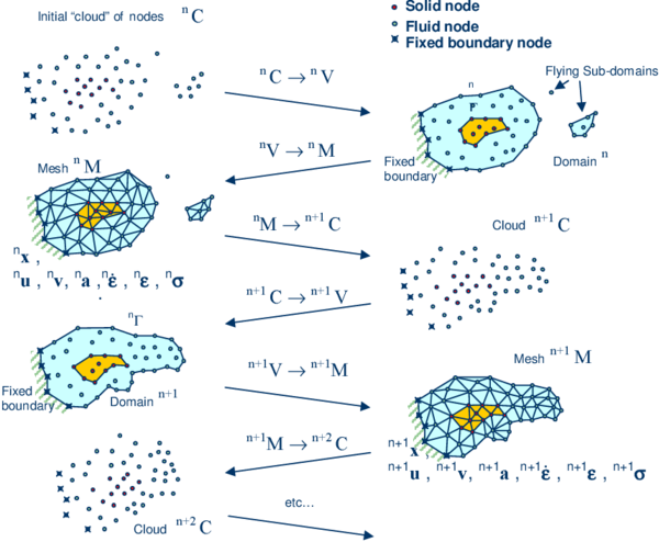
|
| Figure 1: Sequence of steps to update a “cloud” of nodes representing a domain containing a fluid and a solid part from time () to time () |
- The starting point at each time step is the cloud of points in the fluid and solid domains. For instance denotes the cloud at time (Figure 1).
- Identify the boundaries defining the analysis domain , as well as the subdomains in the fluid and the solid. This is an essential step as some boundaries (such as the free surface in fluids) may be severely distorted during the solution, including separation and re-entering of nodes. The Alpha Shape method [8] is used for the boundary definition. Clearly, the accuracy in the reconstruction of the boundaries depends on the number of points in the vicinity of each boundary and on the Alpha Shape parameter. In the problems solved in this work the Alpha Shape method has been implementation as described in [12,28].
- Discretize the the analysis domain with a finite element mesh We use an efficient mesh generation scheme based on an enhanced Delaunay tesselation [11,12].
- Solve the Lagrangian equations of motion for the overall continuum using the standard FEM. Compute the state variables in at the next (updated) configuration for : velocities, pressure and viscous stresses in the fluid and displacements, stresses and strains in the solid.
- Move the mesh nodes to a new position where n+1 denotes the time , in terms of the time increment size.
- Go back to step 1 and repeat the solution for the next time step to obtain .
Note that the key differences between the PFEM and the classical FEM are the remeshing technique and the identification of the domain boundary at each time step.
The CPU time required for meshing grows linearly with the number of nodes. As a general rule, meshing consumes for 3D problems around 15% of the total CPU time per time step, while the solution of the equations (with typically 3 iterations per time step) and the system assembly consume approximately 70% and 15% of the CPU time per time step, respectively. These figures refer to analyses in a single processor Pentium IV PC [36]. Considerable speed can be gained using parallel computing techniques.
In this work we will apply the PFEM to problems involving a rigid domain containing fluid particles only. Application of the PFEM in fluid and solid mechanics and in fluid-structure interaction problems can be found in [4,5,6,8,9,10,11,12,13,14,15,16,17,18,19,28,29,35,36,39,40,41,42,43], as well in www.cimne.com/pfem.
8 EXAMPLES
8.1 Sloshing of water in prismatic tank
The problem has been solved first in 2D. Figure 2 shows the analysis data. The fluid oscillates due to the hydrostatic forces induced by its original position.
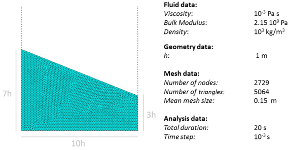
|
| Figure 2: 2D analysis of sloshing of water in rectangular tank. Initial geometry, analysis data and mesh of 5064 3-noded triangles discretizing the water in the tank |
The problem has been run using different values of the parameter in the tangent bulk stiffness matrix (Eq.(41)). The first set of results (Figures 3 and 4) were obtained with . The problem was then solved for , thereby, reducing in one order the magnitude the diagonal terms in .
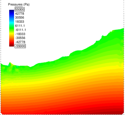
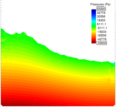
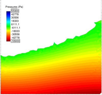
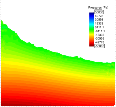
Figure 3 shows snapshots of the water geometry at different times. Pressure contours are superposed to the deformed geometry of the fluid in the figures.
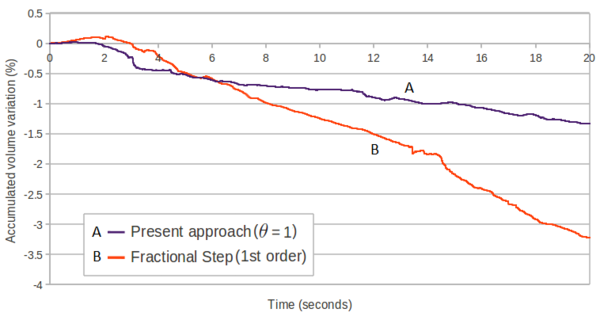
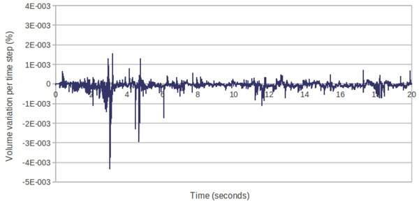
Figure 4 shows the evolution of the percentage of water volume (i.e. mass) loss introduced by the numerical solution scheme. The accumulated volume loss (in percentage versus the initial volume) for the method proposed with is approximately 1.33% over 20 seconds of simulation time (Figure 4a). The average volume variation in absolute value per time step is (Figure 4b). The total water volume loss is the sum of the losses induced by the numerical scheme and the losses due to the updating of the free surface using the PFEM. No correction of mass was introduced at the end of each time step. Taking all this into account, the fluid volume loss over the analysis period is remarkably low.
The volume losses induced by the free surface updating can be reduced using a finer mesh in that region in conjunction with an enhanced alpha shape technique.
The total fluid volume loss can be reduced to almost zero by introducing a small correction in the free surface at the end of each time step [41].
The fluid volume losses obtained using a standard first order fractional step method [41] and the PFEM are shown in Figure 4a for comparison. Clearly the method proposed in this work leads to a reduction in the overall fluid volume loss, as well as in the volume loss per time step.
|
|
| (a) t=5.7s | (b) t=7.4s |
|
|
| (c) t=13.3s | (d) t=18.6s |
| Figure 3: 2D sloshing of water in rectangular tank. Snapshots of water geometry at two different times (). Colours indicate pressure contours | |
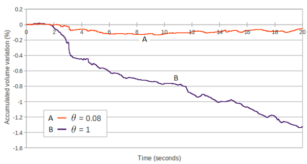
Figure 5 shows a comparison between the fluid volume loss for and using the same time step in both cases (). Results show that the reduction of the tangent bulk stiffness matrix terms leads to an improvement in the preservation of the initial volume of the fluid. It is noted that the convergence of the iterative solution for was the same as for .
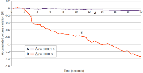
Figure 6 shows that a similar improvement in the volume preservation can be obtained using and reducing the time step to . This, however, increases the cost of the computations.
These results indicate that accurate numerical results with reduced volume losses can be obtained by appropriately adjusting the parameter in the tangent bulk modulus matrix while keeping the time step size to competitive values in terms of CPU cost. A study of the influence of in the numerical solution for quasi-incompressible free surface fluids in terms of volume preservation and overall accuracy using the formulation here presented can be found in [10].
More results for this example can be found in [41].
|
| Figure 5: 2D sloshing of water in rectangular tank. Time evolution of percentage of water volume loss obtained using the current method with (curve A) and (curve B) |
|
| Figure 6: 2D sloshing of water in rectangular tank. Time evolution of percentage of water volume loss obtained with the current method. Curve A: and . Curve B: and |
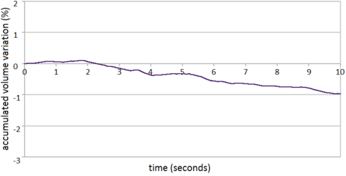
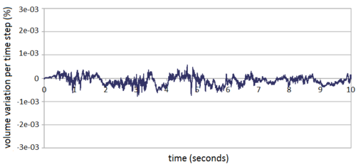
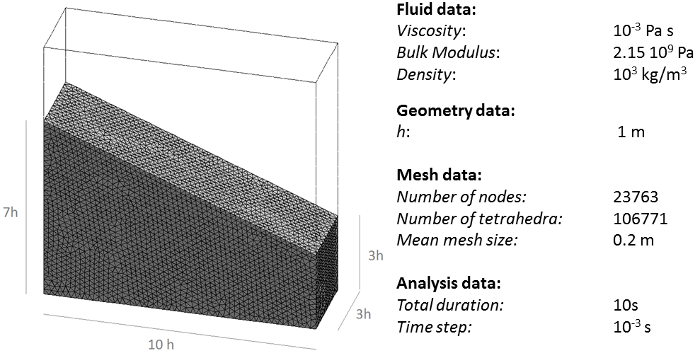
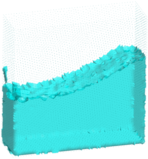
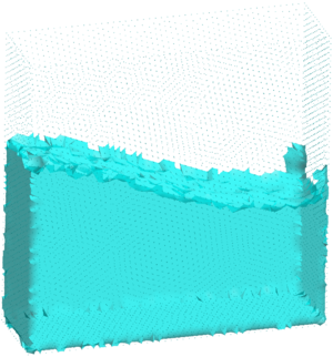
Figures 7 and 8 show a similar set of results for the 3D analysis of the same sloshing problem using a relative coarse initial mesh of 106771 4-noded tetrahedra and . It is remarkable that the percentage of total fluid volume loss due to the numerical scheme after 10 seconds of analysis is approximately 1%.
|
]] | |
|
| |
| (a) t=5.7s | (b) t=7.4s | |
| Figure 7: 3D analysis of sloshing of water in prismatic tank (). Analysis data and snapshots of water geometry at s (a) and s (b) | ||
8.2 Falling of a water sphere in a cylindrical tank containing water
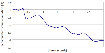
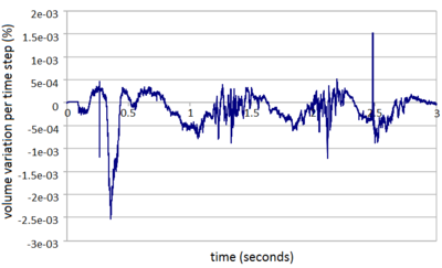
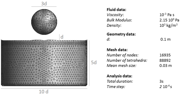
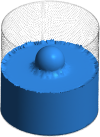
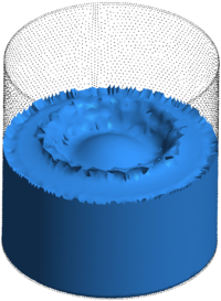
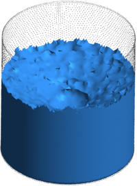
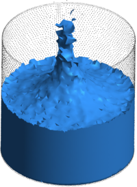
This example is the 3D analysis of the impact of a sphere made of water as it falls in a cylindrical tank containing water. Both the water in the sphere and in the tank mix in a single fluid after the impact. Figure 9 shows the material and analysis data and the initial discretization of the sphere and the water in the tank in 88892 4-noded tetrahedra. The problem was solved with the new stabilized method presented in the paper with . Figure 10 shows snapshots of the mixing process at different times. An average of four iterations for convergence of the velocity and the pressure were needed during all the steps of the analysis. The total water mass lost in the sphere and the tank due to the numerical algorithm was 2% after 3 seconds of analysis (Figure 11a).
|
| Figure 9: Water sphere falling in a tank filled with water. Analysis data and initial discretization of the sphere and the water in the tank with 88892 4-noded tetrahedra |
|
|
| (a) t=0.175s | (b) t=0.275s |
|
|
| (c) t=0.5s | (d) t=0.9s |
| Figure 10: Water sphere falling in tank containing water. Evolution of the impact and mixing of the two liquids at different times. Results for | |
8.3 Sloshing of a fluid in a heated tank
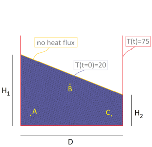
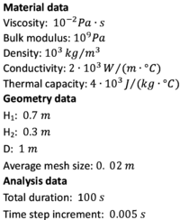
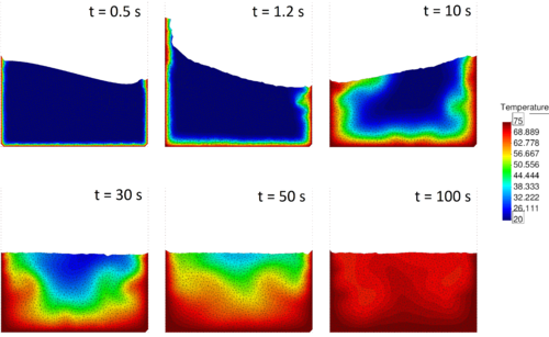
A fluid at initial temperature oscillates due to the hydrostatic forces induced by its initial position in a rectangular tank heated to a uniform and constant temperature of . The geometry and the problem data of the 2D simulation are shown in Figure 12. The fluid, with a very high thermal conductivity, changes its temperature only due to the contact with the hotter tank walls. The heat flux along the free surface has been considered null. The fluid domain has been initially discretized with 2828 3-noded triangles. The coupled thermal-fluid dynamics simulation has been run for 100 s using a time step increment of =.
Figure 13 shows some snapshots of the numerical simulation. The temperature contours have been superposed on the fluid domain at the different time instants.
In Figure 14 the evolution of temperature with time at the points and of Figure 12 is plotted. The coordinates of these sample points are (), () and (), respectively. Figures 13 and 14 show that the fluid does not heat uniformly because of the convection effect automatically captured by the Lagrangian technique here presented.
|
|
| Figure 12: 2D sloshing of a fluid in a heated tank. Initial geometry, problem data, thermal boundary and initial conditions | |
|
| Figure 13: 2D sloshing of a fluid in a heated tank. Snapshots of fluid geometry at six different times. Colours indicate temperature contours |

|
| Figure 14: 2D sloshing of a fluid in a heated tank. Evolution of temperature with time at the points and of Figure 12 |
8.4 Falling of a cylindrical object in a heated tank filled with fluid
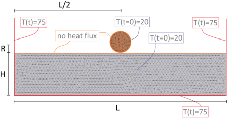
An elastic object falls in a tank containing a fluid at rest. The tank walls are maintained at temperature = during the whole analysis, while the fluid and the solid object have an initial temperature of . The geometry and the problem data of the 2D simulation as well the thermal initial and boundary conditions, are shown in Figure 15. Both the fluid and the solid have a high thermal conductivity. The heat flux along the fluid and solid surfaces in contact with the air has been considered null. The fluid and the solid domains have been discretized with 1986 and 108 3-noded triangular finite elements, respectively. The duration of the simulation is 10 s and the time step increment chosen is =.
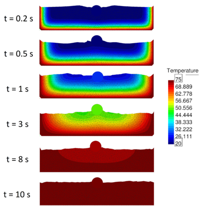
Figure 16 collects some representative snapshots of the numerical simulation with the temperature results plotted over the fluid and the solid domains.
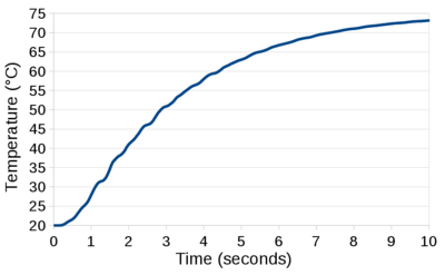
The graph of Figure 17 is the evolution of temperature at the central point of the solid object. As expected, its temperature tends to =.
|

|
| Figure 15: Falling of a solid object in a heated tank filled with fluid. Initial geometry, problem data, thermal boundary and initial conditions |
|
| Figure 16: Falling of a solid object in a heated tank filled with fluid. Snapshots at six different times. Colours indicate temperature contours |
|
| Figure 17: Falling of a solid object in a heated tank filled with fluid. Time evolution of the temperature at the center of the solid. |
9 CONCLUDING REMARKS
We have presented a new FIC-based stabilized Lagrangian finite element method for thermal-mechanical analysis of quasi and fully incompressible flows and FSI problems that has excellent mass preservation properties. The method has been successfully applied to the adiabatic and thermal-mechanical analysis of free-surface quasi-incompressible flows using the PFEM and an updated Lagrangian formulation. These problems are more demanding in terms of the mass preservation features of the numerical algorithm. The method proposed has yielded excellent results for 2D and 3D adiabatic and thermally-coupled free surface flow problems involving surface waves, water splashing, violent impact of flows with containment walls and FSI situations.
ACKNOWLEDGEMENTS
This research was partially supported by the Advanced Grant project SAFECON of the European Research Council.
Bibliography
[1] Aubry R, Idelsohn SR, Oñate E (2005) Particle finite element method in fluid-mechanics including thermal convection-diffusion. Computers and Structures, Vol. 83, (17-18), pp 1459–1475.
[2] Aubry R, Idelsohn SR, Oñate E (2006) Fractional step like schemes for free surface problems with thermal coupling using the Lagrangian PFEM. Computational Mechanics, Vol. 38 (4-5), pp. 294–309.
[3] Belytschko T, Liu WK, Moran B, Non linear finite element for continua and structures, 2d Edition, Wiley, 2013.
[4] Carbonell JM, Oñate E, Suárez B (2010) Modeling of ground excavation with the Particle Finite Element Method. Journal of Engineering Mechanics (ASCE) 136(4):455–463
[5] Carbonell JM, Oñate E, Suárez B (2013) Modelling of tunnelling processes and cutting tool wear with the Particle Finite Element Method (PFEM). Accepted in Comput. Mech. (2013) DOI:10.1007/s00466-013-0835-x
[6] Cremonesi M, Frangi A, Perego U (2011) A Lagrangian finite element approach for the simulation of water-waves induced by landslides. Computers & Structures 89:1086–1093
[7] Donea J, Huerta A (2003) Finite element method for flow problems. J. Wiley
[8] Edelsbrunner H, Mucke EP (1999) Three dimensional alpha shapes. ACM Trans. Graphics 13:43–72
[9] Felippa F, Oñate E (2007) Nodally exact Ritz discretizations of 1D diffusion-absorption and Helmholtz equations by variational FIC and modified equation methods. Comput. Mech. 39:91–111
[10] Franci A, Oñate E, Carbonell JM (2013) On the effect of the tangent bulk stiffness matrix in the analysis of free surface Lagrangian flows using PFEM. Research Report CIMNE PI402. Submitted to Int. J. Numer. Meth. Biomed. Engng.
[11] Idelsohn SR, Calvo N, Oñate E (2003c) Polyhedrization of an arbitrary point set. Comput. Method Appl. Mech. Engng. 192(22-24):2649–2668
[12] Idelsohn SR, Oñate E, Del Pin F (2004) The particle finite element method: a powerful tool to solve incompressible flows with free-surfaces and breaking waves. Int. J. Numer. Meth. Biomed. Engng., 61(7):964–989
[13] Idelsohn SR, Marti J, Limache A, Oñate E (2008) Unified Lagrangian formulation for elastic solids and incompressible fluids: Application to fluid-structure interaction problems via the PFEM. Comput Methods Appl Mech Engrg. 197:1762–1776
[14] Idelsohn SR, Mier-Torrecilla M, Oñate E (2009) Multi-fluid flows with the Particle Finite Element Method. Comput Methods Appl Mech Engrg. 198:2750–2767
[15] Idelsohn SR, Oñate E (2010) The challenge of mass conservation in the solution of free-surface flows with the fractional-step method: Problems and solutions. Int. J. Numer. Meth. Biomed. Engng. 26:1313–-1330
[16] Idelsohn SR, Nigro N, Limache A, Oñate E (2012) Large time-step explicit integration method for solving problem with dominant convection. Comput. Methods Appl. Mech. Engrg. 217-220:168–-185
[17] Larese A, Rossi R, Oñate E, Idelsohn SR (2008) Validation of the Particle Finite Element Method (PFEM) for simulation of free surface flows. Engineering Computations 25(4):385–425
[18] Limache A, Idelsohn, SR, Rossi R, Oñate E (2007) The violation of objectivity in Laplace formulation of the Navier-Stokes equations. Int. J. Numerical Methods in Fluids, 54:639–664.
[19] Oliver X, Cante JC, Weyler R, González C, Hernández J (2007) Particle finite element methods in solid mechanics problems. In: Oñate E, Owen R (Eds) Computational Plasticity. Springer, Berlin, pp 87–103
[20] Oñate E (1998) Derivation of stabilized equations for advective-diffusive transport and fluid flow problems. Comput. Meth. Appl. Mech. Engng. 151:233–267
[21] Oñate E, Manzan M (1999) A general procedure for deriving stabilized space-time finite element methods for advective-diffusive problems. International Journal for Numerical Methods in Fluids, Vol. 31, pp. 203–221.
[22] Oñate E (2000) A stabilized finite element method for incompressible viscous flows using a finite increment calculus formulation. Comput Methods Appl Mech Engrg. 182(1–2):355–370
[23] Oñate E, García J (2001) A finite element method for fluid-structure interaction with surface waves using a finite calculus formulation. Comput. Meth. Appl. Mech. Engrg. 191:635–660
[24] Oñate E (2003) Multiscale computational analysis in mechanics using finite calculus: an introduction. Comput. Meth. Appl. Mech. Engrg. 192(28-30):3043–3059
[25] Oñate E, Taylor RL, Zienkiewicz OC, Rojek J (2003) A residual correction method based on finite calculus. Engineering Computations 20:629–658
[26] Oñate E (2004) Possibilities of finite calculus in computational mechanics. Int. J. Num. Meth. Engng. 60(1):255–281
[27] Oñate E, Rojek J, Taylor R, Zienkiewicz O (2004a) Finite calculus formulation for incompressible solids using linear triangles and tetrahedra. Int. J. Numer. Meth. Engng. 59(11):1473–1500
[28] Oñate E, Idelsohn SR, Del Pin F, Aubry R (2004b) The particle finite element method. An overview. Int. J. Comput. Methods 1(2):267–307
[29] Oñate E, M.A. Celigueta, Idelsohn SR (2006a) Modeling bed erosion in free surface flows by the Particle Finite Element Method, Acta Geotechnia 1(4):237–252
[30] Oñate E, Valls A, García J (2006b) FIC/FEM formulation with matrix stabilizing terms for incompressible flows at low and high Reynold's numbers. Computational Mechanics 38 (4-5):440–455
[31] Oñate E, García J, SR Idelsohn, F. Del Pin (2006c) FIC formulations for finite element analysis of incompressible flows. Eulerian, ALE and Lagrangian approaches. Comput. Meth. Appl. Mech. Engng. 195(23-24):3001–3037
[32] Oñate E, Valls A, García J (2007) Computation of turbulent flows using a finite calculus-finite element formulation. Int. J. Numer. Meth. Engng. 54:609–637
[33] Oñate E, Idelsohn SR, Celigueta MA, Rossi R (2008) Advances in the particle finite element method for the analysis of fluid-multibody interaction and bed erosion in free surface flows. Comput. Meth. Appl. Mech. Engng. 197(19-20):1777–1800
[34] Oñate E (2009) Structural analysis with the finite element method. Linear statics. Volume 1. Basis and Solids. CIMNE-Springer
[35] Oñate E, Rossi R, Idelsohn SR, Butler K (2010) Melting and spread of polymers in fire with the particle finite element method. Int. J. Numerical Methods in Engineering, 81(8):1046–1072
[36] Oñate E, Celigueta MA, Idelsohn SR, Salazar F, Suárez B (2011) Possibilities of the particle finite element method for fluid-soil-structure interaction problems. Computational Mechanics, 48(3):307–318.
[37] Oñate E, Nadukandi P, Idelsohn SR, García J, Felippa C (2011) A family of residual-based stabilized finite element methods for Stokes flows. Int. J. Num. Methods in Fluids, 65 (1-3): 106–134
[38] Oñate E, Idelsohn SR, Felippa C (2011) Consistent pressure Laplacian stabilization for incompressible continua via higher-order finite calculus. Int. J. Numer. Meth. Engng, 87 (1-5): 171–195
[39] Oñate E, Nadukandi P, Idelsohn SR (2014) P1/P0+ elements for incompressible flows with discontinuous material properties. Comput. Meth. Appl. Mech. Engng. 271:185-209
[40] Oñate E, Carbonell JM (2013) Updated Lagrangian finite element formulation for quasi-incompressible fluids. Research Report PI393, CIMNE. Submitted to Comput. Mechanics
[41] Oñate E, Franci A, Carbonell JM (2013) Lagrangian formulation for finite element analysis of quasi-incompressible fluids with reduced mass losses. Int. J. Num. Meth. Fluids, DOI: 10.1002/fld.3870
[42] Ryzhakov P, Oñate E, Rossi R, Idelsohn SR (2012) Improving mass conservation in simulation of incompressible flows. Int. J. Numer. Meth. Engng. 90(12):1435–1451
[43] Tang B, Li JF, Wang TS (2009) Some improvements on free surface simulation by the particle finite element method. Int. J. Num. Methods in Fluids, 60 (9):1032–-1054
[44] Zienkiewicz OC, Taylor RL, Zhu JZ (2005) The finite element method. The basis, 6th Ed., Elsevier
[45] Zienkiewicz OC, Taylor RL (2005) The finite element method for solid and structural mechanics, 6th Ed., Elsevier
[46] Zienkiewicz OC, Taylor RL, Nithiarasu P (2005) The finite element method for fluid dynamics, 6th Ed., Elsevier
Document information
Published on 01/01/2014
DOI: 10.1007/978-3-319-06136-8
Licence: CC BY-NC-SA license
Share this document
claim authorship
Are you one of the authors of this document?
