Revision as of 16:10, 16 January 2017 (view source) Scipediacontent (talk | contribs) ← Older edit		Latest revision as of 17:48, 9 May 2017 (view source) Scipediacontent (talk | contribs)
(5 intermediate revisions by 2 users not shown)
Line 1:		Line 1:
−		+	===Abstract===
−		+
−	''Abstract''	+
	Nowadays, dam safety is becoming more relevant in our society due to the importance of its functions (power generation, water supply, flood control) and the severity of the consequences in case of a serious breakdown. The "safety of hydraulic infrastructures" is one of the priorities according to the R<math display="inline">\& </math>D Spanish State Program which is oriented to social challenges.		Nowadays, dam safety is becoming more relevant in our society due to the importance of its functions (power generation, water supply, flood control) and the severity of the consequences in case of a serious breakdown. The "safety of hydraulic infrastructures" is one of the priorities according to the R<math display="inline">\& </math>D Spanish State Program which is oriented to social challenges.
Line 11:		Line 9:
	The proposed software is validated with a real case: La Baells dam. The computational results have shown excellent agreement with the obtained data during monitoring process.		The proposed software is validated with a real case: La Baells dam. The computational results have shown excellent agreement with the obtained data during monitoring process.
−	''Acknowledgements''	+	===Acknowledgements===
	This master thesis would not have been the same without the help of many people, thus I would like to dedicate them few words.		This master thesis would not have been the same without the help of many people, thus I would like to dedicate them few words.
Line 176:		Line 174:
	{| class="floating_imageSCP" style="text-align: center; border: 1px solid #BBB; margin: 1em auto; width: 100%;max-width: 100%;"		{| class="floating_imageSCP" style="text-align: center; border: 1px solid #BBB; margin: 1em auto; width: 100%;max-width: 100%;"
	|-		|-
−	|[[Image:draft_Content_292531468-numerical_process.png|600px|The four steps of a numerical model.]]	+	|[[Image:draft_Content_292531468-numerical_process.png|400px|The four steps of a numerical model.]]
	|- style="text-align: center; font-size: 75%;"		|- style="text-align: center; font-size: 75%;"
	| colspan="1" | '''Figure 3:''' The four steps of a numerical model.		| colspan="1" | '''Figure 3:''' The four steps of a numerical model.
Line 1,027:		Line 1,025:
	|}		|}
−	Eq.[[#eq-44|44]] requires that matrix '''C''' be easily invertible for an effective implementation. The reduction of the matrix to a diagonal or "lumped" form can be accomplished by various procedures, for instance row-sum <span id='citeF-19'></span>[[#cite-19|[19]]] zhu2005finite. Forward-Euler method is conditionally stable and the stability condition is governed by the thermal diffusivity of the material, and the finite element space <span id='citeF-20'></span>[[#cite-20|[20]]]. Euler method is first-order accuracy in time. The main attraction of an explicit scheme is the fact that a matrix solution is not required and computer storage requirements are minimal.	+	Eq.[[#eq-44|44]] requires that matrix '''C''' be easily invertible for an effective implementation. The reduction of the matrix to a diagonal or "lumped" form can be accomplished by various procedures, for instance row-sum <span id='citeF-19'></span>[[#cite-19|[19,29]]]. Forward-Euler method is conditionally stable and the stability condition is governed by the thermal diffusivity of the material, and the finite element space <span id='citeF-20'></span>[[#cite-20|[20]]]. Euler method is first-order accuracy in time. The main attraction of an explicit scheme is the fact that a matrix solution is not required and computer storage requirements are minimal.
	When <math display="inline">\alpha > 0</math>, a family of implicit methods are produced. Depending on the used value there are different schemes:		When <math display="inline">\alpha > 0</math>, a family of implicit methods are produced. Depending on the used value there are different schemes:

---

Latest revision as of 17:48, 9 May 2017

Abstract

Nowadays, dam safety is becoming more relevant in our society due to the importance of its functions (power generation, water supply, flood control) and the severity of the consequences in case of a serious breakdown. The "safety of hydraulic infrastructures" is one of the priorities according to the R${\textstyle \&}$D Spanish State Program which is oriented to social challenges.

Thanks to recent improvements in the modelling of dams as well as the evolution of computational resources, it is possible to perform more detailed analysis. However, most of commercial software is devoted to more common problems (e.g. buildings, bridges) without considering specific aspects of dams: concrete ageing process, joints during the construction process, contact with the ground or uplift pressure.

The development of a specific application for dam engineering, both for construction phase and operating period, is the main objective of this project. The thesis presents the computational tool, which is based on finite element formulations and solves thermo-mechanical problem using weak coupling, designed for analysing the operating period.

The proposed software is validated with a real case: La Baells dam. The computational results have shown excellent agreement with the obtained data during monitoring process.

Acknowledgements

This master thesis would not have been the same without the help of many people, thus I would like to dedicate them few words.

Firstly, I would like to thank Prof. Eugenio Oñate for giving me the opportunity of becoming a member of CIMNE. I would also like to thank my supervisors M.Sc. Fernando Salazar and Dr. Antonia Larese for their guidance and support during the writing of this thesis. I would like to make these thanks extensive to all the members of Room C6 and C4, particularly to Ignasi, for their wide advices and support. I would also like to thank to Dr. Josep Maria Carbonell and Dr. Jose Manuel González for his patience in my beginning with KRATOS and all provided geometries of dams. I can not forget to mention my friends and colleagues Tomás, Ruben and Vicente, with whom I spent so many hours.

I would like to also give special emphasis to my family, especially my parents and brother, because despite the distance, have always given me their unconditional support.

Finally, I would like to thank to all people that shared their time in one way or other with me; life-long friends; Ana, Fernando, Carlos, Leo, Zito, classmates; Samu, Marc, Eric and Marta and flatmates; Jorge and Martin, whom have helped and supported me not only during this work, but also during the whole master course.

This work has been funded by the Ministry of Economy and Competitiveness under Retos Programme through the grant, RTC-2015-3794-5 - ACOMBO.

1 Introduction

Water is a basic resource for all humans. Nowadays, the earth is not still affected by a lack of water but, according with some researches, this situation will change in a short period of time [1].

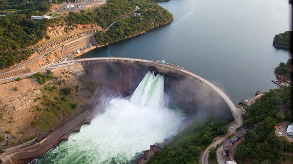
Only 1% of the water in the Earth is freshwater (mainly in rivers, groundwater reserves, lakes and reservoirs, Figure 1 ¹). However, only the reservoirs can be handled by humans. For this reason, dams play an important role in our society.

Figure 1: View of Kariba Dam, the world's biggest reservoir.

Dams are the infrastructures that allow accumulate water with the aim of supply the population, generate energy and control the floods before it arrives to the sea through rivers.

The main objective of a dam is to resist the solicitations that the dammed water generates. This water not only induces a significant mechanical solicitations but also thermal loads due to the gradient of temperatures. Some researches have proved that the influence of the temperature in the global structural response can not be neglected [2].

(¹) http://www.worldbank.org/en/region/afr/brief/the-kariba-dam-rehabilitation-project-fact-sheet

1.1 Motivation

Dam safety is becoming more relevant due to the importance of its functions (power generation, water supply, flood control) and the severity of the consequences in case of a serious breakdown.

In Spain, the majority of the dams were built during last 50 years [3]. For this reason, companies and institutions that are in charge of these structures are worried about the structural response of these critical infrastructures, which is one of the priorities inside the R${\textstyle \&}$D State Program (Programa Estatal de I+D+I Orientada a los Retos de la Sociedad).

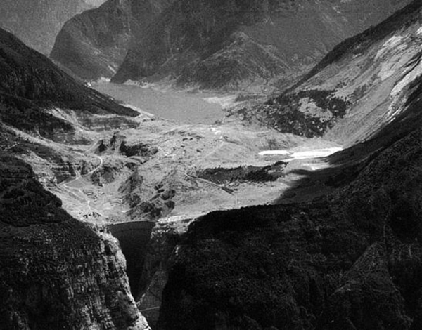
These worries are based on past experiences. The Vajont disaster (Italy)(Figure 2 ¹) is one of the most important and well known. In 1963 an important landslide produced a tsunami which caused 2,000 casualties, however the body of the dam resisted, and today, continues standing [4].

Figure 2: View of Vajont Dam one day after the landslide.

The rainfall generated by Typhoon Nina in Zhumadian (China, 1975) caused the worst disaster originated by dam break in the history. The number of casualties reached the amount of 171,000, and 11 millions of people had to leave their homes. The main factor of this disaster was the extreme conditions generated by the collision of Typhoon Nina and a cold front. The project flood was calculated using a return-period of 1,000 years but that day the flood was the equivalent to a return-period of 2,000 years [5].

During the last 10 years, at least 15 disasters happened around the world, the most important were: Shakidor Dam (Pakistan) in 2005 with 70 casualties, Situ Gintung Dam (Indonesia) in 2009 with 98 casualties, Kyzyl-Agash Dam (Kazakhstan) in 2010 with 43 casualties or Köprü Dam (Turkey) in 2012 reaching 10 casualties.

In this context, the aim of this work is to develop a tool that simulates the real behaviour of dams and predicts its response.

(¹) https://en.wikipedia.org/wiki/Vajont_Dam

1.2 Objectives

The main objective of this thesis is to develop a computational tool for structural verification of dams, including the possibility of thermo-mechanical analysis.

Since the software is specific for dams, the possibility to assign some ad-hoc boundary conditions is implemented, such as the Bofang temperature conditions [6] and the possibility to vary the water level through an input table data.

Another important objective of this thesis is to check whether accurate results can be obtained with tetrahedral elements. Dam structural calculations are typically performed with hexahedral meshes, which are difficult to generate for complex geometries. The use of tetrahedral meshes avoids these problems.

1.3 Structure of the Thesis

The present thesis is divided in six parts. The first one is the Introduction where the motivation and the objectives of the thesis were presented.

Chapter 2 is dedicated to literature review. In this chapter, a general guideline for the use of numerical models in dam engineering [7] are presented, focusing in recommendations for new dams and dealing with particular issues on existing dams.

In chapter 3 the proposed methodology for solving the problem is presented. This chapter deals with the mechanical, thermal and thermo-mechanical formulation. The derivation of the weak formulation is stated as well as the coupling between thermal and mechanical problem.

Chapter 4 is devoted to introduce the KRATOS environment and the Dam Applica- tion. KRATOS is a framework for building multi-disciplinary finite element programs. It provides several tools for easy implementation of finite element applications and a common platform with effortless interaction between them. On the other hand, Dam Application is a new specific application for structural verification of dams. The main implementations, how it works internally and its dependencies of other applications are presented.

Chapter 5 is dedicated to numerical results. La Baells arch Dam was selected as a case study: a numerical model was built and computed via the new Dam Application, and the results were compared to; a) the actual dam behaviour, as measured by the monitoring devices, and b) numerical results obtained with the software COMET.

In Chapter 6 some conclusions about the work performed as well as future work are discussed.

2 Literature Rewiew

The use of numerical tools such as finite element, boundary element and finite difference methods, has become standard practice in dam engineering. There is extensive literature about this subject and a specific document published by the International Commission on Large Dams (ICOLD) in his bulletin 155 [7].

The object of the computational activity is often missed during the process. Due to this fact, it is important to emphasise the different purposes of a numerical simulation of dam-foundation-reservoir:

• Prediction of the structural stability and simulation of any possible failure mechanisms under all types and the whole range of loading scenarios (typically normal operation, flood and earthquake).
• Pre-design and optimization of new dams at different project stages.
• Interpretation of the behaviour of dams under operation by comparison of results of the monitoring system with theoretical computed values.
• Design and optimization of remedial works, corrective measures, and most efficient rehabilitation methods of existing dams,

In the numerical analysis of dams, there are two different scenarios depending on the stage: design of a new structure, or analysis of an existing one. In case of new dams, general recommendations for the process of numerical analysis in this field are presented, in this stage the two first purposes are dealt: prediction of the structural stability and pre-design. In the case of existing dams, special attention to the information provided by the monitoring system and the dealing with the last two commented purposes must be taken. The main distinction between modelling new and existing dam lies on the fact that the numerical models can not be calibrated for a new dam since no information on the actual dam response is available.

2.1 Numerical Models for New Dams

The basic goal of the numerical analysis is to provide adequate answers to a set of relevant questions related to the performance of a dam. Past incidents and failures have confirmed the necessity of this type of studies in the design phase considering all possible scenarios. Several aspects must be taken into account when considering the application of numerical models for design and analysis dams.

The size and refinement of the finite element grid

It is important to remember that a higher finite element density, and correspondingly finite elements of smaller size, is necessary where higher gradients are expected. These high gradients can appear in areas where there are geometrical singularities (e.g. sharp corners), as well as in relation to the loading condition.

The domain dimension around the dam is another important issue regarding the numerical model. This question takes special relevance when dynamic analysis is performed but can not be ignored for static or quasi-static analysis.

The Saint-Venant principle states that a disturbance to a given model has an influence on the stress level in a surrounding domain which has equal to the dimension of the disturbance itself. For static loads and linear analysis, this principle can be applied. Considering the dam as the disturbance, the extension of the surrounding foundation should be at least equal to a characteristic dimension of the structure.

Generally, 2-dimensional models are adopted for embankment dams or straight plant masonry/concrete dams; however, the application of this simplification to other typologies as: curved plant masonry/concrete dams or arch dams can lead to problems. In these typologies of dams the use of 3-dimensional models are needed.

The inclusion of discontinuities

The consideration of discontinuities (e.g. construction joints, interfaces, cracks) demand a non-linear finite element modelling. A preliminary linear elastic analysis in order to check the stress field is always a good idea. With this information it is possible to activate the kinematics (opening or sliding) of the discontinuities. In case of concrete arch dams can not avoid the inclusion of discontinuities.

The definition of the initial stress-strain state

This is one of the most complex problems to be solved for existing structures, not only because of the lack of information on construction but also due to the lack of knowledge on the thermo-visco-mechanical parameters which govern the phenomena.

In traditional numerical modelling, the dead weight of the structure is simulated as an instantly applied load acting on the complete structure to obtain its final conditions at the boundaries. In practice, the dead weight and the stiffness is applied progressively according with the dam construction.

With regards to concrete dams, the consideration of dead weight during the dam construction may be important to evaluate the stress-strain state caused by the generation and dispersion of hydration heat in concrete block masses which are not totally free to contract during the cooling process. In arch dams, the simulation of contraction joints injection could be more significant.

Treatment of consolidation of foundations

The evolution of the effects of this type of process (jet-grouting, cement injection) are quite difficult due to the physical-mechanical characteristics of the rock foundations. Field tests may be useful to evaluate the efficiency of the consolidation works. This information also can be used to prepare the numerical model.

2.1.1 Type of analyses for new projects

In the design phase numerical analysis plays an important role. The design affects the final cost of the project but also the maintenance and the risk are factors that must be taken into account.

Mainly in the design of dams two tools are used: past dam engineering experience (behaviour of existing dams) and the analytical and numerical models. When these conditions are met computational models provide a safe baseline for design of new dams, based on past experience and knowledge with the support of associated design criteria.

In the design of a new dam, most of the information is generally conventional, there is no much data that can be used as project-specific reference. Due to this lack of accurate information, this situation leads to an iterative design process with successive definitions of the project characteristics (dimensions) until a satisfactory degree of optimization is reached.

It is recommendable to perform an analysis in the linear elastic range, even for extreme loading conditions. The goal of this analysis is to identify possible damaged zones.

After carrying out linear analysis, it is recommendable to perform a non-linear study under extreme loading scenarios (severe seismic ground motions) to obtain better approximations of dam behaviour. Non-linear models are not easy to interpret. The main difficult comes from the stress transmission when the strength of the material is reached. This procedure can be corrupted for several reasons:

• Non linear models need to be treated with approximate numerical iterative procedures; in zones close to yielding surface can appear numerical instabilities.
• Even a good mathematical model can produce some differences with the prototype in the plastic range.
• For non-linear models the load history is very important.
• The ultimate behaviour of a structure can be strongly influenced by local weakness of the material.

Non-linear finite element models are a useful tool to capture non-elastic mechanical properties.

The appropriate framework for the numerical analysis process consist of:

• Simplifying.
• Selecting and using the adequate model to get the best answer with available information.
• Checking the consistency between results and assumptions.

Same procedure is suitable for both the design of a new structure and the analysis of an existing one.

2.1.2 The steps of a numerical process

Numerical models can produce a relevant picture of the state of stresses and the displacement field of the structure. Numerical models are essential to comprehend the behaviour of the dam. These models are widely used during the optimization process.

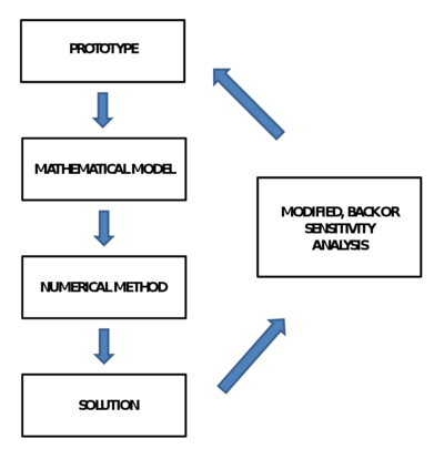
Figure 3 shows the different steps in the numerical model.

• Prototype The physical structure to be analysed with all its complexities.
• Mathematical model A formulation which transfers in mathematical terms the conceptual model representing the behaviour of both the structure to be built and its foundation.
• Numerical method Used to solve the mathematical model and to obtain a numerical solution. Generally, numerical methods provide an approximation of the 'exact solution'.
• Numerical model The solution of the mathematical model by means of the numerical method.
• Evaluation of the solution The translation of the numerical results into practical conclusions.

Figure 3: The four steps of a numerical model.

In many cases this process is iterative. The evaluation of the first case often leads to modify the model, the imposed boundary conditions... when calibrations are possible. In this process the experience of the professionals plays an important role, they must be aware about the assumptions and simplifications used. This is particularly important in non-linear models since the uniqueness of the solution is not guaranteed.

2.1.3 Preliminary design tools

Preliminary designs are based mainly in past experience of the designer with respect to similar dams built. These designs usually have similar conditions: geological, topographical, hydrological and material parameters.

In case of having similar parameters and conditions a simple model can be suitable. On the other hand, when the characteristics are unprecedented (quite often in arch dams) a too simple approach may be insufficient, and should be considered as only initial step. When more information is available a more realistic model is performed.

The numerical analysis of new projects is typically associated with the following challenges:

• Extrapolation from experience represent a large leap, the numerical models must be able to avoid this leap and represent as realistically as possible the phenomena involved.
• The information of materials and loads are not directly available during model calibration, and the values must be obtained through progressive researches. The idea is to start with a simple and unreliable model and arrive to a sophisticated and realistic one.

2.1.4 Methods for in-depth analysis

In the case of extreme scenarios such as Maximum Credible Earthquake or Probable Maximum Flood, more sophisticated models may be necessary to explain this complex behaviour. Clear examples of this necessity can be transient underground seepage, cooling of new concrete, contact between two blocks or two types of materials and dam behaviour during earthquakes.

The aim of non-linear finite elements is the representation of non-linear stress behaviour of soils, concrete, rock foundation, cracks and joints. It is not necessary a global non-linear analysis, since location of non-linearities are known (e.g. dam-foundation contact interface). Another important consideration in the case of global non-linear analysis is that the results are non-unique due to they are dependent on the load-history, the model, and the numerical solution method.

The definition of acceptable safety criteria always requires a correct selection of design parameters since the solution is sensitive to modelling assumptions. Most of safety guidelines are not addressed to establish acceptable margins through the interpretation of finite element results. These factors of safety are sensitive to the calculation techniques.

The stresses are dependent on model discretization and mesh size. A clear example of that can be a heel of a gravity dam subjected to linear elastic analysis. The whole area related to the heel is mesh dependent. There are different techniques to avoid these problems, for example the use of adaptive techniques with the aim of refining the mesh in the affected area. Another possible solution could be the introduction of non-linearities in this area.

Following, the particular issues on existing dams modelling are dealt.

2.2 Particular issues on existing dam modelling

Many of the considerations commented in previous section can be applied to this section. Nonetheless, this section is focused on the relation between the behaviour of the structure and the need of periodic assessment with understanding of the nature, source and relevance of the uncertainties involved.

One of the basic aspects related to existing dams is the surveillance. There are three important phases in the surveillance of dam life: during construction, during first impounding of the reservoir and during the operating period. Monitoring activity is an important ingredient to validate design assumptions, and also can be used to calibrate mathematical models or to detect abnormal deviations for long-term behaviours [8].

Construction

All data provided by monitoring devices are very useful for checking the critical design parameters (e.g. the foundation deformability or hydration heat) and to make corrections during construction phase.

First impounding of the reservoir

In this phase some monitored parameters concerning the dam-foundation-reservoir response to environmental loads with predicted values from design are compared. In case the differences are significant, it is a must the investigation of the origin of these differences and to take corrective measures if needed. This phase is also important in the mathematical model calibration.

Operation

The measurements from the monitoring systems and visual inspections carried out periodically are processed and compared to predicted values. In case of long-term operation, it is also important to check the influence of ageing process in the structure. In the case of detecting an important ageing process, the model must be calibrated. Another important mission of this monitoring process is the detection of behaviour changes and the study of these changes.

2.2.1 Uncertainties of measurements

The obtained data are crucial in the interpretation of dam behaviour. However, the measurements can be under suspicion due to uncertainties linked to the installation, calibrating process or its conservation. In fact, wrong measurements can lead to incorrect decisions, due to this, some dam engineers can be sceptic about their importance [9].

The combination of statistical models and registered data can lead to better understanding of the dam behaviour.

2.2.2 Forecasting Numerical Models

Dams are designed for long time and their require an important investment not only during the construction period but also during the operating period. The surveillance of dams is crucial to avoid future disasters. A failure of a large dam can generate unacceptable casualties and important damages.

Due to above commented facts, there is a necessity to make forecasting models to predict the dam behaviour. The data processing of these predictions with the real data give the possibility of a quick response in case of issues.

Generally, forecasting models are of the following form [10]:

${\displaystyle R(t,env)=P_{h,r}(t,h)+P_{\theta ,r}(t,\theta )+P_{t}(t,h,\theta )+D(t,h,\theta ,env)}$

(1)

where

• ${\textstyle R}$ is the observed value of a given indicator
• ${\textstyle P}$ represents the forecast of the same indicator
• ${\textstyle P_{h,r}}$ is the reversible hydrostatic component
• ${\textstyle P_{\theta ,r}}$ is the reversible thermal component
• ${\textstyle P_{t}}$ is the irreversible component
• ${\textstyle D}$ is the difference between the measurement and the theoretical model. It represents the sum of all the model inaccuracies and/or measurements errors.

The independent variables are:

• ${\textstyle t}$ the time from a given origin
• ${\textstyle h}$ the reservoir water level
• ${\textstyle \theta }$ the material temperature distribution
• ${\textstyle env}$ the environmental variables

There are four different ways for computing the forecasting indicators:

• Deterministic approaches

  These methods are based on mathematical models. The quality of the forecast depends mainly on the capability of the mathematical model to describe the physical reality, the quality of the numerical solution, the knowledge of the parameters describing the materials , the simplifications introduced in the model and the knowledge of the independent variables at the time of observation. They do not need previous measurements, and usually is used for a first reservoir impounding or for the first years of operating.

• Statistical approaches

  A set of influence functions corresponding to expected variation of each indicator is chosen. Each component of each function is multiplied by a parameter or unknown coefficient, and these coefficients are defined with previous measurements. It is necessary the use of an a priori analytical form of the indicators (based on experience). The calibration process is performed through the minimization of a given norm. This technique can be applied to different phenomena.

• Hybrid methods

  These methods combine the above introduced models. By one hand, the analytical form of the indicators is obtained through the deterministic approach, but each single term of the function is multiplied by an unknown coefficient. The calibration is carried out as in statistical approach.

• Neural Networks approaches

  This methodology [11] is relatively new and is inspired by neural networks. The neural networks are composed of many simple intercommunicating units, or neurons, working in parallel to solve a given problem. It expands as the network learns to operate, based on a set of training data provided by users. Nowadays, several types of neural techniques exist, the most important one in the back analysis is the multi-layer feed-forward and back-propagation algorithm. These methods have lot of potential.

2.2.3 Monitoring systems

The surveillance of a dam is mainly performed by visual inspections carried out by qualified personal and by processing data obtained from monitoring devices.

Most of dangerous events as sinkholes, settlements, cracks, concentrated seepages, generally can not be detected by monitoring devices and must be detected through visual inspections. When an abnormal behaviour is detected, its evolution can be surveyed and analysed on the basis of the data collected by a monitoring system suitable installed. The parameters provided by the monitoring devices can be grouped in two categories: environmental actions and the physical-mechanical quantities describing the response of the dam-foundation-reservoir.

• Environmental actions

  Inside this group it is possible to find the following quantities: reservoir water level, air temperature, water temperatures at different depths in the reservoir, solar radiation, seismic actions, rainfall...

• Response of the dam-foundation-reservoir

  In this group it is necessary to distinguish between different typology of dams:

• Concrete dams: absolute displacements of the dam foundation, relative displacements between blocks, temperature evolution in the dam body, strains...
• Embankment dams: displacements and especially settlement of the dam-foundation system during dam construction and operation, leakages, seepages, pore pressures in the waterproof core...

It is important to remind that the monitoring devices tends to modify and disrupt their local value, especially in quantities like strains and stresses.

Thanks to the important growth of electromechanical devices and advances in topic of the transmission data, this information each time is more relevant and easy to access.

2.2.4 Numerical methods for structural identification

The basic idea of any structural identification method is to make a numerical model behaviour as close as possible to the observed one.

The structural identification methods can be based on static and dynamic monitoring data.

• Static data

  These methods are basically those already shown in previous section 2.2.2: the calibration step usually performed to set up forecasting models may be seen as identification process which allows evaluating the best estimate of the physical/mechanical parameters of the dam-foundation system.

• Dynamic data

  Dynamic methods have taken more importance in last decades. These methods are based on dynamic excitation. The aim of the dynamic structural identification consist in the evaluation of the dynamic features (e.g. natural frequencies, modal shapes) according to excitation (input) and response (output) of the system. This process is performed through dynamic campaigns. The structural response can be measured in terms of acceleration, velocity or displacement vs. time. Depending on the available devices, the measurement is carried out in one term or other. According to the measured parameter a different range of frequencies must be used (e.g. velocity measurements requires low frequencies).

The excitation of the structure can be obtained in a different ways depending on the available resources, the importance of the structure...

• The most expensive and reliable solution is to apply one exciter on the structure (e.g. hydraulic piston). The exciters are controlled in terms of frequencies and amplitudes. This approach is strongly recommended in dams (massive structure).
• Environmental vibrations is a cheap method but the problem resides in that the signal could be corrupted, moreover long acquisition times must be planned in order to remove noise.
• Others methods as "pull ${\textstyle \&}$ release" test or the impact test can be applied as alternatives.

The selection of a proper method is very important so that no damage are induced on the structure during the test. To this aim is highly recommended a previous evaluation to predict the amplitudes on the model.

The selection of an adequate mathematical algorithm for identification is very important, and the following aspects must be taken into account:

• The more physical characteristics are included into mathematical models the more accurate is the identification process.
• At the end of the identification, the mathematical model must be able to properly capture the true physical aspects of the system.

Frequency and/or modal shapes may be used directly for matching and error minimization, as already was mentioned before for time domain identification.

The extension of a dynamic analysis to a non-linear field must be done carefully and considering the following differences:

• The natural frequencies and modal shapes of a non-linear systems are dependent on the amplitude of response.
• The dependence of the natural frequencies and modal shapes can be used to refine identification estimates and to help localizing non-linear effects and corresponding damages.
• Some non-linear systems may be "uncoupled" in order to make easier identification and analysis.

Summing up, structural identification not only provides a powerful diagnostic tool but also a refined system to support a deep understanding of the dam behaviour.

3 Methodology

In this chapter the used methodology is presented. Due to the nature problem the structure of the chapter is divided in three sections: mechanical, thermal and thermo-mechanical problem.

The first section deals to the mechanical problem focusing in Linear Elasticity Theory, a branch of General Elasticity Theory. In this section the governing equations of the mechanical problem as well as the weak formulation and the numerical integration techniques are presented. In second section the thermal problem is stated. Same structure than in previous section is followed. Finally, the thermo-mechanical problem with a weak coupling is introduced.

Many of the concepts discussed below are dealt extensively in the book of Prof. Eugenio Oñate, Structural Analysis with the Finite Element Method. Linear Statics [12] [13],as well as in the book of Prof. Xavier Oliver and Prof. Carlos Agelet de Saracibar, Mecánica de medios continuos para ingenieros [14].

3.1 Mechanical Problem

Usually, a mechanical problem can be defined in the following way; given an initial geometry and a loading field, analyse the response according to a stiffness and strength. For solving the problem is necessary to state the basic equations.

• Equilibrium equations
• Constitutive equations
• Compatibility equations

Depending on the constitutive equation the solid behaviour is different. The following models describe how a solid responds to an applied force:

• Elastic: when a solid starts to suffer strains, it increases the elastic potential energy which means that its internal energy increases avoiding irreversible transformations. The main feature is a reversible process; if the acting forces are removed the solid recuperates the initial shape.
• Plastic: materials that behave elastically when the applied stress is less than a yield value. When the stress is greater than the yield stress the material behaves plastically and does not return to its previous state. That is, deformation that occurs after yielding is permanent.
• Viscous: this type of behaviour happens when the strain velocity acts in the constitutive equation. The behaviour can also be elastic or plastic.

This study is focused in Linear elasticity since the approximation that it provides is good enough for the purpose. Most of engineering problems can be solved using this type of hypothesis.

Linear elasticity is the mathematical study of how solid objects deform and become internally stressed due to prescribed loading conditions. Linear elasticity is a simplification of the more general non-linear theory of elasticity and is a branch of continuum mechanics.

The fundamental "linearizing" assumptions of linear elasticity are[14]:

• Infinitesimal strains: displacement and its gradient are small enough.

• Small displacements. There is no difference between material and spatial configuration.
• Small displacements gradient. There is no difference between the Green-Lagrange Strain tensor E(X,t) and the Almansi Strain tensor e(x,t) and are equal to infinitesimal strain tensor ${\textstyle {\boldsymbol {\varepsilon }}({\textbf {x}},t)}$.

• Existence of neutral state: exists a state where strains and stresses have zero value, usually this state is assumed as the reference configuration.
• The deformation process is isothermal and adiabatic.

• Isothermal: process in where the temperature is constant along the time.
• Adiabatic: process that not generates heat in any point at any time.

3.1.1 Governing Equations

The solution for elastic problems can be stated through two different approaches depending on the unknown variable;

• Displacements
• Stresses

In this thesis, a displacement approach is used, but in the cases where the contour stresses are known, the use of Beltrami-Michell approach is reasonable. Nonetheless, there are mixed formulations that allow to solve the problem without the necessity of knowing all stresses [15].

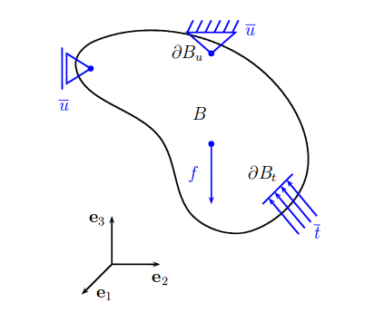
In direct tensor form, the governing equations for a linear elastic problem are [14]:

• Cauchy Equation;

${\displaystyle \nabla \cdot {\boldsymbol {\sigma }}+\rho _{0}{\textbf {b}}=\rho _{0}{\ddot {\textbf {u}}}}$

(2)

• Constitutive equation;

${\displaystyle {\boldsymbol {\sigma }}=\lambda Tr(\varepsilon ){\textbf {1}}+2\nu \varepsilon }$

(3)

• Compatibility equations;

${\displaystyle {\boldsymbol {\varepsilon }}=\nabla ^{s}{\textbf {u}}={\frac {1}{2}}({\textbf {u}}\otimes \nabla +\nabla \otimes {\textbf {u}})}$

(4)

The boundary conditions and the initial conditions are

${\displaystyle \partial B_{u}:{\textbf {u}}={\textbf {u}}^{*}}$ ${\displaystyle \partial B_{\sigma }:{\textbf {t}}^{*}={\boldsymbol {\sigma }}\cdot {\textbf {u}}^{*}}$ ${\displaystyle {\textbf {u}}({\textbf {x}},0)={\textbf {0}}}$ ${\displaystyle {\dot {\textbf {u}}}({\textbf {x}},0)={\textbf {v}}_{0}}$

(5)

Figure 4: Scheme of generic problem in linear elasticity.

3.1.2 Analysis Type

Regarding the analysis type, there are three important groups:

• Static. This analysis is time independent. The forces are gradually applied and remain in place for longer duration of time.
• Quasi-static. This analysis is time dependent but it takes the assumptions that the loads are applied slow enough to neglect acceleration terms.

${\displaystyle {\textbf {a}}={\frac {\partial {\textbf {u}}({\textbf {x}},t)}{\partial t^{2}}}\approx {\textbf {0}}}$

(6)

• Dynamic. This analysis is time dependent without simplifications. Dynamic loads are very much time dependent, either for acting in a small interval of time or quickly change in magnitude or direction. Some examples of dynamics loads are: earthquakes, machinery vibrations...

Depending on the analysis type, the system to be solved is different. The most common analysis types are: quasi-static and dynamic.

Using a Finite Element Method and a quasi-static analysis, the system reads as

${\displaystyle {\textbf {K}}{\textbf {u}}={\textbf {f}}}$

(7)

where K is the stiffness matrix, u is the vector of displacements and f is the vector forces.

In case of dynamic analysis, the system becomes more complex and reads like

${\displaystyle {\textbf {M}}{\ddot {\textbf {u}}}+{\textbf {C}}{\dot {\textbf {u}}}+{\textbf {K}}{\textbf {u}}={\textbf {f}}}$

(8)

where M is the mass matrix, C is the damping matrix and, ${\textstyle {\ddot {\textbf {u}}}}$ and ${\textstyle {\dot {\textbf {u}}}}$ are acceleration and velocity vector, respectively.

In this thesis, due to the considered loads are not influenced by the time, the analysis type is quasi-static.

3.1.3 Finite Element Model

The Finite Element Method (FEM) is a numerical technique for finding approximate solutions to boundary value problems for partial differential equations. It uses subdivisions of a whole problem domain, and variational methods to solve the problem by minimizing an associated error function.

The main concept is connect many simple element equations over many small domains to approximate a more complex equation over a larger domain. Although continuum structures are always three-dimensional, if the proper simplification hypothesis are fitted, one can accurately describe the behaviour of a structure by means of uni or bi-dimensional mathematical models, like in earth dams, tunnels, etc.

Next, the generic stages for the analysis of a structure through the Finite Element Method are presented. Assuming a quasi-static analysis, the equilibrium equation in strong form can be stated as

${\displaystyle \nabla \cdot {\boldsymbol {\sigma }}+\rho {\textbf {b}}={\textbf {0}}}$

(9)

In solid mechanics, the six stress components can be computed through the six components of strain (${\textstyle \varepsilon }$) which are computed from the displacements

${\displaystyle {\textbf {u}}=[u,\;v,\;w]^{T}}$

(10)

To obtain the weak form an arbitrary weight function vector 11 is introduced

${\displaystyle {\textbf {v}}=\delta {\textbf {u}}=[\delta u,\;\delta v,\;\delta w]^{T}}$

(11)

and the equation is integrated over whole domain

${\displaystyle \int _{V}\delta {\textbf {u}}^{T}(\nabla \cdot {\boldsymbol {\sigma }})\;dV+\int _{V}\delta {\textbf {u}}^{T}\rho {\textbf {b}}\;dV={\textbf {0}}}$

(12)

after applying the divergence theorem is obtained

${\displaystyle \int _{V}\nabla \delta {\textbf {u}}^{T}{\boldsymbol {\sigma }}\;dV=\int _{V}\delta {\textbf {u}}^{T}\rho {\textbf {b}}\;dV+\int _{A}\delta {\textbf {u}}^{T}{\boldsymbol {\sigma }}\cdot {\textbf {n}}\;dA}$

(13)

introducing the concept of virtual strains that can be stated as the derivation of virtual displacements ${\textstyle \nabla \delta {\textbf {u}}=\delta \varepsilon }$

${\displaystyle \int _{V}\delta {\boldsymbol {\varepsilon }}^{T}{\boldsymbol {\sigma }}\;dV=\int _{V}\delta {\textbf {u}}^{T}\rho {\textbf {b}}\;dV+\int _{A}\delta {\textbf {u}}^{T}{\boldsymbol {\sigma }}\cdot {\textbf {n}}\;dA}$

(14)

which is the three-dimensional equivalent virtual work statement.

The virtual displacements and the virtual strains are interpolated in terms of the virtual displacement values in the standard form

${\displaystyle \delta {\textbf {u}}={\textbf {N}}\delta {\textbf {a}}\qquad ;\qquad \delta {\boldsymbol {\varepsilon }}={\textbf {B}}\delta {\textbf {a}}}$

(15)

Substituting and simplifying the virtual displacements

${\displaystyle \iiint _{V^{(e)}}{\textbf {B}}^{T}{\boldsymbol {\sigma }}\;dV=\iiint _{V^{(e)}}{\textbf {N}}^{T}\rho {\boldsymbol {b}}\;dV+\iint _{A^{(e)}}{\textbf {N}}^{T}{\textbf {t}}\;dA}$

(16)

where B and N are the strain matrix and the shape function matrix, respectively. Using the stresses expression

${\displaystyle {\boldsymbol {\sigma }}={\textbf {C}}\;{\boldsymbol {\varepsilon }}={\textbf {C}}\;{\textbf {B}}{\textbf {a}}^{(e)}}$

(17)

finally the following equation is obtained

${\displaystyle \left[\iiint _{V^{(e)}}{\textbf {B}}^{T}{\textbf {C}}{\textbf {B}}\;dV\right]{\textbf {a}}^{(e)}=\iiint _{V^{(e)}}{\textbf {N}}^{T}\rho {\boldsymbol {b}}\;dV+\iint _{A^{(e)}}{\textbf {N}}^{T}{\textbf {t}}\;dA}$

that can also be expressed as

${\displaystyle {\textbf {K}}^{(e)}\;{\textbf {a}}^{(e)}={\textbf {f}}^{(e)}}$

(18)

where

${\displaystyle {\textbf {K}}^{(e)}=\iiint _{V^{(e)}}{\textbf {B}}^{T}{\textbf {C}}{\textbf {B}}\;dV}$

(19)

is the elastic stiffness matrix of the element, and

${\displaystyle {\textbf {f}}^{(e)}={\textbf {f}}_{b}^{(e)}+{\textbf {f}}_{t}^{(e)}}$

(20)

the nodal vector force. The nodal vector is composed by the body forces and tractions forces, but may also be other contributions. These concepts and the way to compute the stiffness and the vector force are detailed in Appendix A.

To finish, the global system is constructed

${\displaystyle {\textbf {K}}\;{\textbf {a}}={\textbf {f}}}$

(21)

and solved for the unknown variable, the nodal displacement vector. Once it is obtained, it is quite straightforward to calculate the strains ${\textstyle \varepsilon }$ and stresses ${\textstyle \sigma }$ at each element as well as the reactions at the nodes with prescribed displacements.

3.1.4 Integration Schemes

Integration schemes are methods to integrate differential equations. There are two groups of integration schemes; explicit and implicit.

The explicit schemes use the previous step solution (${\textstyle t_{n}}$) to compute the current step solution (${\textstyle t_{n+1}}$), these types of schemes are conditionally stable and require that the time step size ${\textstyle \Delta t}$ be less or equal than a critical time step. The critical time step depends on element size and maximum wave speed for element material. In some cases, this value has to be too small and requires high number of steps to reach the reality, driving to high computational effort.

The implicit schemes use previous step solution (${\textstyle t_{n}}$) and current step solution (${\textstyle t_{n+1}}$) to compute the current solution. Generally, an implicit solution is unconditionally stable [16], and the used time step can be one or two orders of magnitude larger than in an explicit schemes. However, the accuracy of the implicit schemes deteriorates as the time step increases relative to the period of response of the system.

In this work two well known numerical integration schemes are presented: Newmark method and Bossak method, which is an extension of Newmark method.

Newmark-${\displaystyle \beta }$ Method This method is widely used in numerical evaluation of the dynamic response of structures and solids [17]. Originally, this method is from 1959 but some improvements have been developed. In matrix form the linear dynamic equilibrium equations can be written as

${\displaystyle {\textbf {M}}{\ddot {\textbf {u}}}_{n+1}+{\textbf {C}}{\dot {\textbf {u}}}_{n+1}+{\textbf {K}}{\textbf {u}}_{n+1}={\textbf {f}}_{n+1}}$

(22)

Using truncated Taylor's series as two additional equations expressed in the following form

${\displaystyle {\textbf {u}}_{n+1}={\textbf {u}}_{n}+\Delta t{\dot {\textbf {u}}}_{n}+{\frac {\Delta t^{2}}{2}}{\ddot {\textbf {u}}}_{n}+\beta \Delta t^{3}{\overset {...}{\textbf {u}}}}$ ${\displaystyle {\dot {\textbf {u}}}_{n+1}={\dot {\textbf {u}}}_{n}+\Delta t{\ddot {\textbf {u}}}_{n}+\gamma \Delta t^{2}{\overset {...}{\textbf {u}}}}$

(23)

and assuming linear acceleration within the time step

${\displaystyle {\overset {...}{\textbf {u}}}={\frac {({\ddot {\textbf {u}}}_{n+1}-{\ddot {\textbf {u}}}_{n})}{\Delta t}}}$

(24)

it is just necessary to substitute Eq.24 into Eq.23 to produce Newmark’s equations in standard form

${\displaystyle {\textbf {u}}_{n+1}={\textbf {u}}_{n}+{\dot {\textbf {u}}}_{n}+(0.5-\beta )\Delta T^{2}{\ddot {\textbf {u}}}_{n}+\beta \Delta t^{2}{\ddot {\textbf {u}}}_{n+1}}$ ${\displaystyle {\dot {\textbf {u}}}_{n+1}={\dot {\textbf {u}}}_{n}+(1-\gamma )\Delta t{\ddot {\textbf {u}}}_{n}+\gamma \Delta t{\ddot {\textbf {u}}}_{n+1}}$

(25)

It is known that values of ${\textstyle \gamma }$=0.5 and ${\textstyle \beta }$=0.25 make an unconditionally stable method. The use of values of ${\textstyle \gamma }$ higher than 0.5 introduces errors associated to numerical damping.

Bossak Method

The Bossak method is the extension of the Newmark method. The acceleration ${\textstyle {\ddot {\textbf {u}}}}$ is taken prior to ${\textstyle n+1}$. The method can successfully replace the Newmark method in all cases, and can be stated as

${\displaystyle {\textbf {M}}(1-\alpha _{B}){\ddot {\textbf {u}}}_{n+1}+{\textbf {M}}\alpha _{B}{\ddot {\textbf {u}}}_{n}+{\textbf {C}}{\dot {\textbf {u}}}_{n+1}+{\textbf {K}}{\textbf {u}}_{n+1}={\textbf {f}}_{n+1}}$ ${\displaystyle {\textbf {u}}_{n+1}={\textbf {u}}_{n}+{\dot {\textbf {u}}}_{n}+(0.5-\beta )\Delta T^{2}{\ddot {\textbf {u}}}_{n}+\beta \Delta t^{2}{\ddot {\textbf {u}}}_{n+1}}$ ${\displaystyle {\dot {\textbf {u}}}_{n+1}={\dot {\textbf {u}}}_{n}+(1-\gamma )\Delta t{\ddot {\textbf {u}}}_{n}+\gamma \Delta t{\ddot {\textbf {u}}}_{n+1}}$

(26)

The use of ${\textstyle \alpha _{B}}$=0 leads to Newmark method. The Bossak method is characterized by a good damping in high frequencies range.

3.1.5 Solution Strategies

The used strategy is typically from non-linear problems, but also can be applied to linear ones. One of the main features of linear elasticity is the uniqueness of solution, however in non-linear problems there is a lack of uniqueness of the solution. In fact, in many cases the correct solution is path dependent, so it depends on the path followed.

In matrix form a non-linear problem (given a prescribed boundary conditions and having applied the particular time discretization) can be stated as

${\displaystyle {\textbf {K}}({\textbf {u}}){\textbf {u}}={\textbf {f}}({\textbf {u}})}$

(27)

where u represents the vector of unknowns, K the 'stiffness matrix', and f the force vector, both K and f depend on the solution u. Because of u is unknown, this system is solved by some iterative algorithm, for instance the Newton-Raphson method.

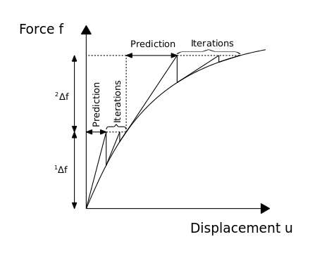
Figure 5: Example of an incremental-iterative method.

Figure 5 shows an incremental iterative method. In incremental iterative methods there is a part of prediction and a part of iteration. The iterations continue until reach some prescribed tolerance. There are different types of convergence criteria depending the case.

Before each solution, the Newton-Raphson method evaluates the out-of-balance load vector, which is the difference between the restoring forces (the loads corresponding to the element stresses) and the applied loads. Then, a linear solution is performed using the out-of-balance loads, and it is checked for a prescribed convergence criterion. If the convergence criterion is not satisfied, the out-of-balance load vector is re-evaluated, the stiffness matrix is updated, and a new solution is obtained. This iterative procedure continues until the problem converges.

The Picard's method is also a famous iterative method for solving non-linear problems, it is computationally cheap but the convergence is very slowly, on the other hand, Newton-Raphson requires higher computational cost but the rate of convergence is higher.

3.2 Thermal Problem

The thermal problem is governed by classical heat equation. In dam engineering, the thermal problem takes on special importance due to the temperature variation in different seasons. The temperature field inside of the dam can be predicted solving the diffusion problem. Once the temperature field inside of the dam is obtained, its gradient can be computed.

The energy equation for a solid in a vector form can be stated as [18]

${\displaystyle \rho C{\frac {\partial \theta }{\partial t}}=\nabla \cdot (k\nabla \theta )+Q}$

(28)

where ${\textstyle \rho }$ is the density, ${\textstyle C}$ is the specific heat, ${\textstyle k}$ is the thermal conductivity and ${\textstyle Q}$ is the rate of heat generation.

Neglecting the heat generation term (since the system does not generate its own heat per unit volume), and arranging terms, the equation reads as

${\displaystyle {\frac {\partial \theta }{\partial t}}={\frac {k}{\rho C}}\nabla ^{2}\theta }$

(29)

the above equation is known as heat equation. The thermal diffusivity (${\textstyle \alpha }$) is obtained dividing the thermal conductivity between the density and the specific heat. Finally, the equation reads as

${\displaystyle {\frac {\partial \theta }{\partial t}}=\alpha \nabla ^{2}\theta }$

(30)

Once the governing equation is obtained, the boundary conditions and the initial conditions are introduced. Boundary conditions are given by

${\displaystyle -(k\;\nabla \theta )\cdot {\textbf {n}}=q_{a}+q_{b}+q_{c}}$

(31)

where ${\textstyle q_{a}}$ is an applied flux, ${\textstyle q_{c}}$ is the convective flux and ${\textstyle q_{r}}$ is the radiative flux, which are dependent on the convective heat transfer coefficient and the effective radiation heat transfer coefficient, respectively

${\displaystyle q_{c}=h_{c}(s_{k},\theta ,t)(\theta {-\theta }_{c})\qquad ;\qquad q_{r}=h_{r}(s_{k},\theta ,t)(\theta {-\theta }_{r})}$

(32)

The initial condition on the temperature is given by

${\displaystyle \theta ({\textbf {x}},0)=\theta _{0}({\textbf {x}})}$

(33)

3.2.1 Finite Element Model

The governing equation of the thermal problem in a strong form has been presented, now, the way to obtain the weak formulation of this equation is introduced. Due to it is a linear problem, the material coefficients does not depend on temperature. These assumptions can be taken into account since the variation of the temperature is supposed not too much high. In other type of problems in which the variation of the temperature is high, the problem must be considered temperature dependent.

Using Eq.28, neglecting the heat generation term, multiplying by a test function ${\textstyle w({\textbf {x}})}$, and integrating over the element, the following expression is obtained

${\displaystyle \int _{V}w\;\rho C{\frac {\partial \theta }{\partial t}}\;dV-\int _{V}k\;w\;\nabla ^{2}\theta \;dV=0}$

(34)

after, the divergence theorem is applied

${\displaystyle \int _{V}w\;\rho C{\frac {\partial \theta }{\partial t}}\;dV+\int _{V}k\;\nabla \theta \;\nabla w\;dV-\int _{A}w\;k\nabla \theta \cdot {\textbf {n}}\;dA=0}$

(35)

Applying Fourier's law, the rate of flow of heat energy per unit area through a surface is proportional to the negative temperature gradient across the surface ${\textstyle {\textbf {q}}=-k\nabla \theta }$, the following expression is obtained

${\displaystyle \int _{V}w\;\rho C{\frac {\partial \theta }{\partial t}}\;dV+\int _{V}k\;\nabla \theta \cdot \nabla w\;dV=-\int _{A}w\;{\textbf {q}}\cdot {\textbf {n}}\;dA}$

(36)

Now, assuming that the time dependence can be separated from the spatial variation, the finite element approximation can be stated as

${\displaystyle \theta ({\textbf {x}},t)\simeq ({\textbf {N}})^{T}{\boldsymbol {\theta }}}$

(37)

where ${\textstyle {\textbf {N}}}$ is the vector of shape functions and ${\textstyle {\boldsymbol {\theta }}}$ is a vector of nodal temperatures. Finally, making the substitution of ${\textstyle w({\textbf {x}})={\textbf {N}}(x)}$ according with weak-form Galerkin, the following expression is obtained

${\displaystyle \int _{V}\rho C{\textbf {N}}\cdot {\textbf {N}}^{T}{\dot {\boldsymbol {\theta }}}\;dV+\int _{V}k\;\nabla {\textbf {N}}\cdot \nabla {\textbf {N}}^{T}\;{\boldsymbol {\theta }}dV=\int _{A}{\textbf {N}}\;(q_{a}+q_{c}+q_{r})\;dA}$

(38)

in matrix form reads as

${\displaystyle {\textbf {C}}{\dot {\boldsymbol {\theta }}}+{\textbf {K}}{\boldsymbol {\theta }}={\textbf {Q}}}$

(39)

where C is the specific heat matrix, K is the conductivity matrix, Q is the vector of heat fluxes, ${\textstyle {\boldsymbol {\theta }}}$ is the vector of nodal temperatures and ${\textstyle {\dot {\boldsymbol {\theta }}}}$ is the time rate of the nodal temperatures.

3.2.2 Integration Schemes

The ordinary differential Eq.39 should be integrated with respect to time to obtain a transient response. In general, it is not possible to integrate these equations analytically, so they are approximated in time to obtain a set of algebraic equations in terms of the nodal temperature.

The most popular used method for diffusion problems is called ${\textstyle \alpha }$-family and it consists of the following approximation

${\displaystyle {\dot {\theta ^{a}}}={\frac {1}{\Delta t}}(\theta ^{n+1}-\theta ^{n})}$ ${\displaystyle \theta ^{a}=(1-\alpha )\theta ^{n}+\alpha \theta ^{n+1}}$

(40)

substituting Eq.40 in Eq.39

${\displaystyle {\frac {1}{\Delta t}}{\textbf {C}}({\boldsymbol {\theta }}^{n+1}-{\boldsymbol {\theta }}^{n})+{\textbf {K}}\left[(1-\alpha ){\boldsymbol {\theta }}^{n}+\alpha {\boldsymbol {\theta }}^{n+1}\right]={\textbf {Q}}}$

(41)

and rearranging terms the equation can be expressed as

${\displaystyle {\frac {1}{\Delta t}}{\textbf {C}}{\boldsymbol {\theta }}^{n+1}+\alpha {\textbf {K}}{\boldsymbol {\theta }}^{n+1}={\frac {1}{\Delta t}}{\textbf {C}}{\boldsymbol {\theta }}^{n}-(1-\alpha ){\textbf {K}}{\boldsymbol {\theta }}^{n}+{\textbf {Q}}}$

(42)

The choice of ${\textstyle \alpha =0}$ produces the forward euler scheme, an explicit method which is conditionally stable

${\displaystyle {\frac {1}{\Delta t}}{\textbf {C}}{\boldsymbol {\theta }}^{n+1}={\frac {1}{\Delta t}}{\textbf {C}}{\boldsymbol {\theta }}^{n}-{\textbf {K}}{\boldsymbol {\theta }}^{n}+{\textbf {Q}}}$

(43)

and may be rearranged to clearly show its explicit nature

${\displaystyle {\boldsymbol {\theta }}^{n+1}={\boldsymbol {\theta }}^{n}+\Delta t\left[{\textbf {C}}^{-1}{\textbf {Q}}-{\textbf {C}}^{-1}{\textbf {K}}{\boldsymbol {\theta }}^{n}\right]}$

(44)

Eq.44 requires that matrix C be easily invertible for an effective implementation. The reduction of the matrix to a diagonal or "lumped" form can be accomplished by various procedures, for instance row-sum [19,29]. Forward-Euler method is conditionally stable and the stability condition is governed by the thermal diffusivity of the material, and the finite element space [20]. Euler method is first-order accuracy in time. The main attraction of an explicit scheme is the fact that a matrix solution is not required and computer storage requirements are minimal.

When ${\textstyle \alpha >0}$, a family of implicit methods are produced. Depending on the used value there are different schemes:

• ${\textstyle \alpha =1/2}$ Crank-Nicolson Scheme. Unconditionally stable and second-order accuracy.
• ${\textstyle \alpha =2/3}$ Galerkin Scheme. Unconditionally stable and first-order accuracy.
• ${\textstyle \alpha =1}$ Backward Euler Scheme. Unconditionally stable and first-order accuracy.

Inside the code ${\textstyle \alpha }$ is an input parameter which leads to one scheme or other. Computations have been performed using ${\textstyle \alpha =1}$, backward Euler scheme, and reads like

${\displaystyle \left[{\frac {1}{\Delta t}}{\textbf {C}}+{\textbf {K}}\right]{\boldsymbol {\theta }}^{n+1}={\frac {1}{\Delta t}}{\textbf {C}}{\boldsymbol {\theta }}^{n}+{\textbf {Q}}}$

(45)

Next, the solution strategies for this type of problems are introduced.

3.2.3 Solution Strategies

The discretization in time and space has already presented, now, some strategies to solve the problem are presented. The linear problems do not require iterative solution. These problems just require a matrix solution.

Nonetheless, the non-linear problem using a backward Euler is presented, and the system reads like

${\displaystyle \left[{\frac {1}{\Delta t}}{\textbf {C}}({\boldsymbol {\theta }}^{n+1})+{\textbf {K}}({\boldsymbol {\theta }}^{n+1})\right]{\boldsymbol {\theta }}^{n+1}={\frac {1}{\Delta t}}{\textbf {C}}({\boldsymbol {\theta }}^{n+1}){\boldsymbol {\theta }}^{n}+{\textbf {Q}}({\boldsymbol {\theta }}^{n+1})}$

(46)

In case of dealing with non-linear equations (Eq.46), the use of predictor-corrector, extrapolation methods, and quasi-linearization can often reduce the computational effort at each step without reducing the accuracy of the method.

A quasi-linearization is good choice for mild non-linearities and modest time steps. The system reads like

${\displaystyle \left[{\frac {1}{\Delta t}}{\textbf {C}}({\boldsymbol {\theta }}^{n})+{\textbf {K}}({\boldsymbol {\theta }}^{n})\right]{\boldsymbol {\theta }}^{n+1}={\frac {1}{\Delta t}}{\textbf {C}}({\boldsymbol {\theta }}^{n}){\boldsymbol {\theta }}^{n}+{\textbf {Q}}({\boldsymbol {\theta }}^{n})}$

(47)

which is now a single-step (a non iterative method). Another choice is the use of an extrapolation procedure. Usually, it gives better solution than quasi-linearization and allows a larger time step. The extrapolation procedure takes the following form

${\displaystyle \left[{\frac {1}{\Delta t}}{\textbf {C}}({\boldsymbol {\theta }}^{*})+{\textbf {K}}({\boldsymbol {\theta }}^{*})\right]{\boldsymbol {\theta }}^{n+1}={\frac {1}{\Delta t}}{\textbf {C}}({\boldsymbol {\theta }}^{*}){\boldsymbol {\theta }}^{n}+{\textbf {Q}}({\boldsymbol {\theta }}^{*})}$

(48)

where

${\displaystyle {\boldsymbol {\theta }}^{*}={\frac {3}{2}}{\boldsymbol {\theta }}^{n}-{\frac {1}{2}}{\boldsymbol {\theta }}^{n-1}}$

(49)

In case of strong non-linearities, these techniques do not offer accurate results. In these cases, the coupling of a forward Euler predictor with a corrector is a viable option [21][22].

3.3 Thermo-Mechanical Problem

Two different problems need to be solved: a mechanical problem and a thermal problem. There are different approaches to do so, but the most common are probably two: the fully coupling and the one-way coupling.

The fully coupling is usually reserved to solve problems in which both the mechanical and thermal components can affect each other in a similar way. In order to deal with this kind of problems one needs to solve the two components at the same time, taking into account the interaction between them. Among others, this approach is used in the solution of metal forming deposition and additive manufacturing. In this sort of situations, the material properties change dramatically in time and so it is crucial that both components are fully coupled so as to properly capture the real behaviour of the medium. In the case of additive manufacturing, for instance, the higher temperatures reached during the process of binder generate a totally different material behaviour as compared to that encountered in the cooling process.

On the other hand, the one-way coupling technique is devoted for those problems in which the interaction between both parts exists, but it is not symmetric. In essence, one of the components has a strong influence on the other, but the contrary does not occur. This is the case of dams, where the mechanical problem is really affected by the temperature changes, but the thermal problem is almost insensible to the deformation of the geometry.

Next, the main features of the latter coupling are introduced.

3.3.1 One-way coupling

First, the diffusion problem is solved, once it is solved, instead to consider an elastic problem, a thermoelastic problem taking into account the influence of the temperatures through the constitutive law is considered.

The main difference between linear thermoelasticity and linear elasticity is that the process is not considered isothermal any more. The temperature value changes along the time ${\textstyle \theta ({\textbf {x}},t)}$, it means

${\displaystyle \theta ({\textbf {x}},t)\neq \theta ({\textbf {x}},0)=\theta _{0}}$ ${\displaystyle {\dot {\theta }}({\textbf {x}},t)={\frac {\partial \theta ({\textbf {x}},t)}{\partial t}}\neq 0}$

(50)

Nonetheless, the hypothesis of adiabatic process is still considered.

3.3.1.1 Linear thermoelastic constitutive law

The thermal contribution are added to the stresses as

${\displaystyle {\boldsymbol {\sigma }}={\textbf {C}}\;{\boldsymbol {\varepsilon }}-{\boldsymbol {\beta }}(\theta -\theta _{0})}$

(51)

where ${\textstyle {\textbf {C}}}$ is the constitutive matrix, ${\textstyle {\boldsymbol {\beta }}}$ is the thermal properties matrix and ${\textstyle \theta _{0}}$ is the reference temperature field. Usually, the difference between temperatures is written as ${\textstyle \Delta \theta }$.

3.3.1.2 Linear thermoelastic inverse constitutive law

Eq.51 can be inverted to obtain the relation of the strains and it reads as

${\displaystyle {\boldsymbol {\varepsilon }}={\textbf {C}}^{-1}{\boldsymbol {\sigma }}+\Delta \theta {\textbf {C}}^{-1}{\boldsymbol {\beta }}}$

(52)

The definition of thermal expansion coefficient is

${\displaystyle {\boldsymbol {\alpha }}={\textbf {C}}^{-1}{\boldsymbol {\beta }}}$

(53)

In case of isotropic material, the thermal expansion coefficient becomes a scalar.

3.3.1.3 Thermal stresses and strains

Taking the assumption of working with an isotropic material (case study), the relations between thermal and non-thermal for stresses and strains are presented

• Stresses

${\displaystyle {\boldsymbol {\sigma }}={\boldsymbol {\sigma }}^{nt}-{\boldsymbol {\sigma }}^{t}}$ ${\displaystyle {\boldsymbol {\sigma }}^{nt}=\lambda Tr({\boldsymbol {\varepsilon }}){\textbf {1}}+2\mu \varepsilon }$ ${\displaystyle {\boldsymbol {\sigma }}^{t}=\beta \Delta \theta {\textbf {1}}}$

(54)

• Strains

${\displaystyle {\boldsymbol {\varepsilon }}={\boldsymbol {\varepsilon }}^{nt}+{\boldsymbol {\varepsilon }}^{t}}$ ${\displaystyle {\boldsymbol {\varepsilon }}^{nt}=-{\frac {\nu }{E}}Tr({\boldsymbol {\sigma }}){\textbf {1}}+{\frac {1+\nu }{E}}{\boldsymbol {\sigma }}}$ ${\displaystyle {\boldsymbol {\varepsilon }}^{t}=\alpha \Delta \theta {\textbf {1}}}$

(55)

4 KRATOS and Dam Application

KRATOS is designed as an Open-Source framework for the implementation of numerical methods for the solution of engineering problems. It is written in C++ and is designed to allow collaborative development by large teams of researchers focusing on modularity as well as on performance [23] [24].

The KRATOS features a "core" and "applications" approach where "standard tools" (such as linear algebra or search structures) come as a part of the core. They are available as building blocks in the development of "applications" which focus on the solution of the problems of interest. Its ultimate goal is to simplify the development of new numerical methods.

Figure 6: KRATOS' Logo.

A new application called Dam Application (${\textstyle DamApp}$) has been created due to an specific necessity. This Application is focused in dam engineering. Its main features as; how the application works or what are the dependencies are described below.

${\textstyle DamApp}$ has dependencies of Solid Mechanics Application, Convection-Diffusion Application and in less measure of Poromechanics Application. Figure 7 shows the basic flowchart of the application.

Convection-diffusion Application, as its own name shows is an application for solving convection-diffusion problems, it is in charge of Dr. Pablo Becker. Solid Mechanics Application is devoted to solve all type of problems related solid mechanics, it is in charge of Dr. Josep Maria Carbonell. Poromechanics Application solves pore-pressure problems and the responsible is Ing. Ignasi de Pouplana. I would like to thank all of them for allowing me to use their code.

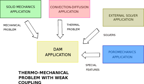
Figure 7: Dam Application's dependencies.

Apart from computational features, a basic but powerful interface where boundary conditions, materials and elements are taken into account has been created. This interface works in GiD, which is a universal, adaptive and user-friendly pre and post processor for numerical simulations in science and engineering [25].

Figure 8 shows the flowchart for solving a generic problem.

Figure 8: Flowchart for solving a generic problem.

4.1 Dam Application

${\textstyle DamApp}$ borns with the aim of solving a real necessity in world of dam engineering. It provides user-friendly interface and specific conditions for dam problems. Internally, it solves a thermo-mechanical problem using a weak coupling.

For solving the thermal problem, the Convection-diffusion Application is used. Since the convective part is not considered in the problem, all its contributions are set to zero, leading to a diffusive problem. After solving the thermal problem for a given time, the mechanical problem taking into account the influence of thermal contribution through the constitutive law must be solved.

Following lines are devoted to present ${\textstyle DamApp}$. The structure is the following; first, the interface is introduced, then the specific boundary conditions of dams are commented, and finally the main files are presented.

4.1.1 Interface

The interface is a powerful tool to define all required information for solving the problem. The development of a correct interface leads to a better understanding and use of the software. A simple but powerful interface has been developed.

The interface is based on the classical problemtype of GiD (Figure 9)

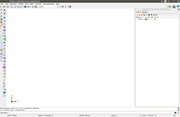
Figure 9: GiD interface

Figure 10 shows the divisions of the main menu. Concretely, the menu is divided in six points:

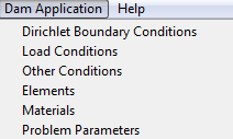
Figure 10: Dam Application menu interface.

• Dirichlet Boundary Conditions, inside of this menu, prescribed displacements and temperatures for different type of entities can be assigned.
• Load Conditions, in this section, it is possible to assign all load conditions to different entities, among others: hydrostatic pressure, normal forces, uplift pressure...
• Other Conditions, inside of this tab it is possible to assign mechanical and thermal properties for solving the thermal problem. The body accelerations can also be assigned in this tab.
• Elements, this section is devoted to assign the type of elements.
• Materials, inside of this menu the materials can be assigned. There are default materials, but it is possible the creation of new materials.
• Problem Parameters, inside of this section the general parameters of the problem can be set. There are some tabs inside of this menu which are the following ones:

• General Data
• Imposed Conditions
• Table Evolution Data
• Mechanical Solver
• Postprocess

4.1.1.1 Dirichlet Boundary Conditions

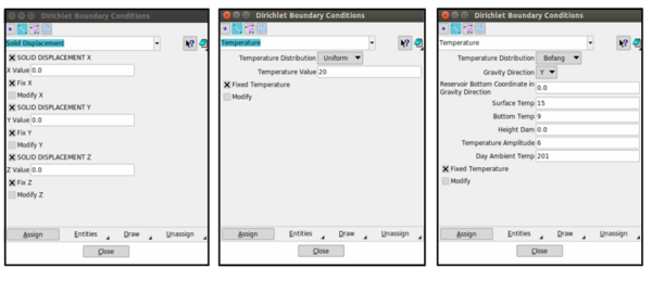
The displacements and temperatures field can be assigned in this menu. The appearance of menu is shown in Figure 11.

Figure 11: Interface menu for applying displacements and temperatures.

4.1.1.2 Load Conditions

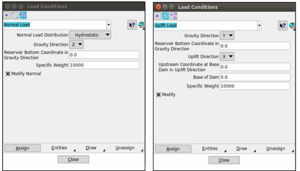
This section is devoted to the application of forces (Figure 12). Several types of forces have been implemented. The user must be aware that there are some limitations, for instance in a 3D view it is not possible to apply a line normal load since the normal direction can not be computed. Below, the different possibilities of loads that can be applied are introduced.

• Point: point load.
• Line: line load, normal load (uniform and hydrostatic) and uplift load.
• Surface: surface load, normal load (uniform and hydrostatic) and uplift load.

Figure 12: Interface menu for applying load conditions.

4.1.1.3 Other Conditions

In this section mechanical and thermal conditions related to the materials can be applied. These conditions are needed due to the Convection-diffusion Application works with nodal variables. Gravitational or acceleration effects can also be assigned in this menu.

4.1.1.4 Elements

This section is dedicated to assign the discrete elements. For instance, in a 2D case it is possible to use linear triangles and quadrilaterals, and also high order elements. In 3D analysis, the possibilities are linear tetrahedrons and hexahedrons as well as high order elements.

It is worth to remark that the thermo-mechanical problem only can be solved by triangles or tetrahedrons since the thermal problem is only implemented for this type of elements. Facing a mechanical problem the user can use any type of element.

4.1.1.5 Materials

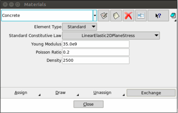
Material assignation is performed in this section. Figure 13 shows the different possibilities for this assignation. Some default materials are ready to use, although if is convenient, the user has the possibility to create new materials. Through the definition of the constitutive law the type of problem (mechanical, thermal or thermo-mechanical problem) is specified.

Figure 13: Interface menu for applying materials.

4.1.1.6 Problem Parameters

To finish this section, the different tabs inside of the Problem Parameters menu are presented.

• General Data

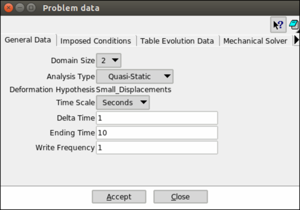
  In this menu (Figure 14), the domain size of the problem, the analysis type (quasi-static or dynamic), the time scale and the temporal values are defined.

Figure 14: Interface menu: General Data.

• Imposed Conditions

  This menu (Figure 15) is the responsible to keep the conditions constant (Unmodified) along time or update them at some point (Table Interpolation).

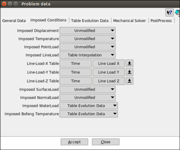
Figure 15: Interface menu: Imposed Conditions.

There are some special conditions as water load and Bofang temperature that are governed by other table Table Evolution Data, this table is explained in the following section.

• Table Evolution Data

  For computing more than one case, it is possible to use this table (Figure 16). The needed values are the following ones: the month in which the computations are carried out (Bofang formulation), the evolution of the water level along the time, the temperature in the not wet wall upstream and the reference temperature.

Figure 16: Interface menu: Table Evolution Data.

• Mechanical Solver

  In this menu (Figure 17), some parameters about the mechanical solver can be set: number of maximum iterations until the convergence is reached, the tolerance of the DOF's and for the residual, the linear solver (direct or iterative) and its type, and finally the number of threads.

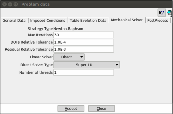
Figure 17: Interface menu: Mechanical Solver.

• Postprocess

  This menu (Figure 18) is devoted for selecting the output parameters. According to interest outputs one or another are selected.

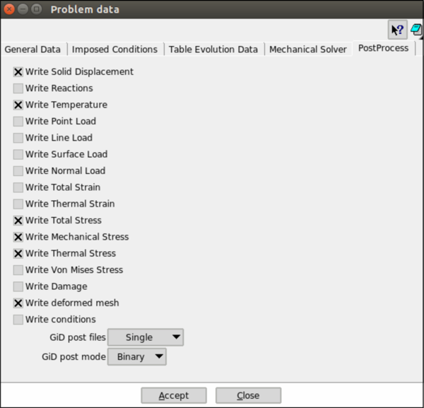
Figure 18: Interface menu: Postprocess.

4.1.2 Boundary Conditions

One of the most remarkable features of the ${\textstyle DamApp}$ is the possibility to apply the following conditions:

• Bofang Temperature
• Hydrostatic Pressure
• Uplift Pressure

These conditions are wide used in dam engineering. In this subsection, how these conditions have been implemented and its relevance are commented.

4.1.2.1 Bofang Temperature

In the upstream wet wall, it is possible to approximate its temperature to the temperature inside of the reservoir.

Up to some years ago, in many research articles, Stucky formulation [26] was used to provide a temperature field, but this temperature field is not too much realistic. Other approaches combine computational fluid dynamics and heat transfer models [27], however, these approaches are complex and computationally expensive.

Analytical models are other alternative to high computation approaches. These approximations are straightforward and its formulation is quite simple. Inside this analytical models, the Bofang formulation has taken important relevance [2]. The Bofang formulation provides a temperature field inside of the reservoir according to an atmospherics input parameters. It is worth to remark that depth of the dam must be higher than 30m, otherwise, the results can be inappropriate.

The proposal of Bofang formulation Bofang is depending on time and depth

${\displaystyle T(y,\tau )=T_{m}(y)+A(y)cos[\omega (\tau -\tau _{0}-\varepsilon )]}$

(56)

where

• ${\textstyle y=depth(m)}$

• ${\textstyle \tau }$ = time (months)

• ${\textstyle T(y,\tau }$) = water temperature at depth y and time ${\textstyle \tau }$

• ${\textstyle T_{m}(y)}$ = yearly mean temperature at depth y (${\textstyle ^{\circ }}$C)

• ${\textstyle A(y)}$ = amplitude of annual variation of water temperature at y-depth

• ${\textstyle \tau _{0}=}$ day of maximum temperature (converted to months)

• ${\textstyle \varepsilon }$ = phase difference of annual variation of water temperature and air temperature

• ${\textstyle \omega =2\pi /P}$ circular frequency of temperature variation

• ${\textstyle P}$ = period of temperature variation (12 months)

Once the general form of Bofang formulation Eq.56 has been presented, the contribution of each part is introduced.

• The yearly mean water temperature

The yearly mean water temperature (${\textstyle T_{m}(y)}$) varies with the ${\textstyle depth-y}$ and may be expressed by

${\displaystyle T_{m}(y)=\left({\frac {T_{b}-T_{s}e^{-0.04H}}{1-e^{-0.04H}}}\right)+\left(T_{s}-{\frac {T_{b}-T_{s}e^{-0.04H}}{1-e^{-0.04H}}}\right)e^{-0.04H}}$

(57)

where

• ${\textstyle T_{s}}$ = yearly mean water temperature at the surface of reservoir

• ${\textstyle T_{b}}$ = yearly mean water temperature at the bottom of reservoir

• ${\textstyle H}$ = depth of reservoir (m)

The way to obtain these parameters is explained in following lines.

In the case of the surface temperature (${\textstyle T_{s}}$), it has to be computed in the following way. In regions where the surface of the reservoir does not freeze in winter, the yearly mean water temperature at the surface is computed by the yearly mean air temperature plus an increment due to solar radiation. In cold regions, the yearly mean air temperature must be modified. The modification consist on set a 0${\textstyle ^{\circ }}$C the temperatures lower than 0${\textstyle ^{\circ }}$C. According with observed data ${\textstyle \Delta b\approx 2^{\circ }C}$.

${\displaystyle T_{s}=T_{a}+\Delta b}$

(58)

In the case of the bottom temperature (${\textstyle T_{b}}$), these temperatures are computed as the mean of the mean value of the air temperature in the three months in the winter.

${\displaystyle T_{b}={\frac {T_{1}+T_{2}+T_{12}}{3}}}$

(59)

• Amplitude of Annual Variation of Water Temperature

The amplitude of annual variation of water temperature (${\textstyle A(y)}$) is the highest at the surface of reservoir and decreases with the depth of water. It may be expressed as

${\displaystyle A(y)=A_{0}e^{-0.018y}}$

(60)

where ${\textstyle A_{0}}$ is the amplitude of variation at the surface of reservoir. Normally, this amplitude can be computed as the mean of maximum (${\textstyle T_{\gamma }}$) and minimum (${\textstyle T_{l}}$) monthly mean air temperature. Usually, in the Northern Hemisphere, these values belongs to the mean air temperature of July and January, respectively.

${\displaystyle A_{0}=(T_{\gamma }-T_{l})/2}$

(61)

In cold regions is computed as

${\displaystyle A_{0}={\frac {T_{\gamma }}{2}}+\Delta a}$

(62)

where ${\textstyle \Delta a}$ is the increment of amplitude due to solar radiation.

• Phase Difference of Variation of Water Temperature ${\displaystyle \varepsilon }$

The phase difference of annual variation of water temperature depends on the depth of water. In case of working in months, it is suggested to compute as

${\displaystyle \varepsilon =2.15-1.30e^{-0.085y}}$

(63)

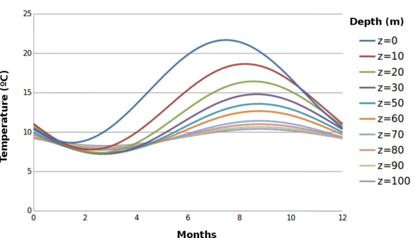
• Applying Bofang Formulation

To understand in a better way how this formulation works, an application example is shown. Figure 19 shows the temperature variation according the period of the year and the depth. The input parameters are described below

${\displaystyle T_{s}=15.19;\;\;T_{b}=9.33;\;\;A_{0}=6.51;\;\;H=100;\;\;\omega =0.52333;\;\;t_{0}=6.5}$

Figure 19: Application of Bofang Formulation.

The temperature at the surface and just below it suffers high variations depending on the period of the year while in deeper levels remains much more constants without barely variations.

The application of this formulation in a real case is presented hereafter. The case study is La Baells dam and the input parameters are

${\displaystyle T_{s}=15.19;\;\;T_{b}=9.33;\;\;A_{0}=6.51;\;\;H=93;\;\;\omega =0.52333;\;\;t_{0}=6.5}$

Figure 20 shows the temperature field in two different seasons when the reservoir is full (${\textstyle H=93m}$). In January (Figure 20a) the variation barely reaches 3${\textstyle ^{\circ }}$C while in July (Figure 20b) it is possible to observe that the variation between the surface and the bottom is amount 12${\textstyle ^{\circ }}$C.

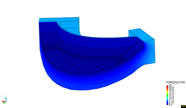
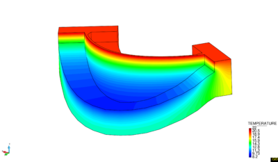
(a) January	(b) July
Figure 20: Application of Bofang Formulation at La Baells dam.

This condition has been implemented in two different program languages: ${\textstyle Basic}$ and ${\textstyle C++}$. The first language is used to write the input file (${\textstyle .mdpa}$), the second one for updating conditions at each time step. There are two different ways to update the conditions: interpolate evolution (given two times, the evolution is computed according an interpolation law) or exact evolution (the condition only changes when the current time arrives to a determined time). The implementation of the developed code in C++ is stated in Appendix C.

4.1.2.2 Hydrostatic Pressure

A fluid in a resting state generates forces on the walls and bottom parts of the container and also on the surfaces of any object submerged. These generated forces are perpendicular to container's walls or any submerged object's surface regardless of the face's direction.

This pressure depends on the density of fluid and the reference height of the measurement. The absolute pressure can be computed as

${\displaystyle P=\rho gh+P_{0}}$

(64)

where

• ${\textstyle P}$ = hydrostatic pressure (${\textstyle Pa}$ or ${\textstyle N/m^{2}}$)

• ${\textstyle \rho }$ = density (${\textstyle kg/m^{3}}$)

• ${\textstyle g}$ = gravity acceleration (${\textstyle m/s^{2}}$)

• ${\textstyle h}$ = is the height of the fluid (${\textstyle m}$)

• ${\textstyle P_{0}}$ = Atmospheric pressure (${\textstyle Pa}$ or ${\textstyle N/m^{2}}$)

Many times it works with relative pressure, neglecting the atmospheric contribution. The application of this condition is performed by the application of nodal forces according to the water level and the coordinates of the nodes.

Below two application examples are shown. The scene of application is La Baells dam. Figure 21a shows the hydrostatic pressure (Pa) with 40m of water level, and outside of water the applied force is equal to 0. In the case of Figure 21b, the water level is equal to 93m, it means that the reservoir is full.

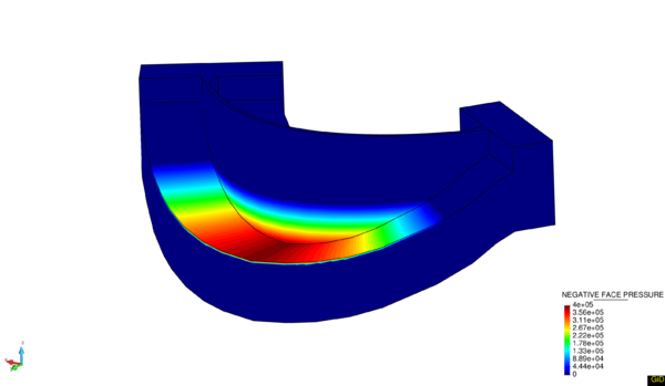
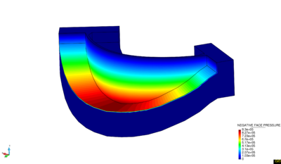
(a) Water level = 40 m	(b) Water level = 93 m
Figure 21: Application of Hydrostatic Pressure at La Baells dam.

The same procedure for coding this boundary condition than in previous case has been followed. The developed code in ${\textstyle C++}$ can be found in Appendix C. As in previous case, there are two ways of updating the conditions; exact or interpolated. It is worth to remark that this file also updates the conditions for uplift pressure.

4.1.2.3 Uplift Pressure

Uplift pressure is a phenomenon very relevant in gravity dams, in arch dams this phenomenon is less important. In gravity dams, the uplift pressure has special importance due to the length of the base is relevant.

Uplift pressure can be defined as the force that is generated due to the seepage in saturated soils at the foundations. These forces act in the base of the structures. Uplift pressure can play an important role in the stability of the structure because it represents a destabilized force.

There are several approaches to compute the uplift pressure. Usually, to know this force, using the flow it is possible to draw the pressure's diagrams, or it is also possible to compute the force using numerical techniques.

The following approach of the uplift pressure has been implemented. In the upstream part the same force than in the lower part of the reservoir is assigned, and this distribution is decreasing until it arrives to 0 at the end of the length of the base. Figure 22 shows this approximation.

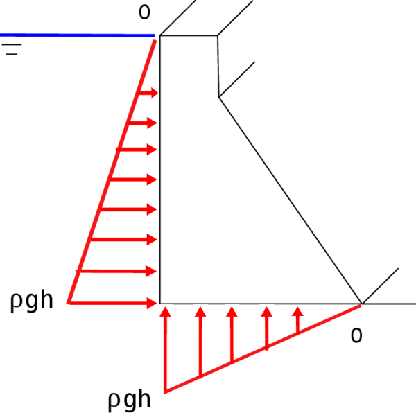
Figure 22: Scheme of uplift pressure approximation.

The formulation to compute the law is

${\displaystyle P=\rho gh*\left[(1.0-\left({\frac {1}{base}}\mid x-x_{ref}\mid \right)\right]}$

(65)

The proposal formulation is related with the water level, it means that in the part that are in contact with the reservoir, the value of the uplift pressure is maximum and it decreases until arrive to 0. It is a must to provide the coordinates in the uplift direction of the upstream to perform the computations.

In arch dams this phenomenon does not take special relevance, and due to the arch geometry, it is a must the modification of the reference coordinate to apply the law properly making harder the application of this type of boundary condition for the user.

Figure 23 shows the application of hydrostatic and uplift pressure in a gravity dam. In the bottom of the upstream there is a matching in values between hydrostatic and uplift pressure.

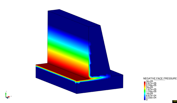
Figure 23: Hydrostatic and Uplift pressure in a gravity dam.

As it has been already commented in previous section, the implemented code can be found in Appendix C.

4.1.3 Main Files

4.1.3.1 Model Part and Project Parameters

The ${\textstyle Model\;Part}$ or also known as ${\textstyle .mdpa}$ is the file that contains all the information related to geometry and boundary conditions of our problem; the mesh (nodes and elements), the applied boundary conditions, the assigned materials, sub-meshes for updating conditions, and tables. On the other hand the ${\textstyle Project\;Parameters}$ file has information about General Data; domain size, ${\textstyle \Delta t}$, type of solver...

The ${\textstyle .mdpa}$ file is written by ${\textstyle Dam_{a}pplication.bas}$ file. This file is the responsible to translate all applied specifications during the pre-process in a script file. A small sample of the ${\textstyle .mdpa}$ file is shown below.

Begin ModelPartData
//VARIABLE_NAME value
End ModelPartData

Begin Table 1 TIME DISPLACEMENT_X
0.00000e+00 0.00000e+00
End Table

Begin Properties  1
CONSTITUTIVE_LAW_NAME  LinearElastic3D
DENSITY                2.50000e+03
YOUNG_MODULUS          3.50000e+10
POISSON_RATIO          2.00000e-01
End Properties

Begin Nodes
1  0.00000e+00 4.00000e+01 1.00000e+01
2  2.00000e+00 4.00000e+01 1.00000e+01
3  0.00000e+00 3.80000e+01 1.00000e+01
4  0.00000e+00 4.00000e+01 8.00000e+00
End Nodes

Begin Elements SmallDisplacementThermoMechanicElement3D4N
1  1  12658 12754 12598 13227
2  1  16536 16594 16471 16462
3  1  15255 15426 15541 15161
4  1  12848 12341 12013 12122
End Elements

In the case of the ${\textstyle Project\;Parameters}$ file, the responsible of the generation of the input file is ${\textstyle 1_{D}am_{A}pplication_{P}arameters.bas}$. A small part of the ${\textstyle ProjectParameter.py}$ file is detailed below.

## General Data ––––––––––––––––––
domain_size = *GenData(Domain_Size,INT)
NumberofThreads = *GenData(Number_of_threads,INT)
time_scale = "*GenData(Time_Scale)"
evolution_type = "*GenData(Evolution_Type)"
delta_time = *GenData(Delta_Time)
ending_time = *GenData(Ending_Time)

These files are not included in Appendix C due to its extension. In case of interest, these files can be found in https://kratos.cimne.upc.es/projects/kratos/repository/show/kratos/applications/DamApplicationKRATOS repository.

4.1.3.2 Thermo_mechanic_script.py

Once the input data have been generated, these are read by the main script. This script (${\textstyle thermo_{m}echanic_{s}cript.py}$) is composed by different stages for solving the problem. In the following lines the different stages are presented.

• Initializing time ${\displaystyle \&}$ Import modules

  The time is initialized and all necessary modules are imported, also the mechanical and thermal solver are defined.

• Previous definitions

  The time parameters, scale of times and output variables are defined.

• Model Part

  The ${\textstyle Model\;Part}$ file (that previously has been generated) is called, and the unknown variables are added to the solver, according the ${\textstyle Project\;Parameters}$ inputs. The ${\textstyle Model\;Part}$ is read and all information about mesh and conditions are extracted. The degrees of freedom are added to the solvers (thermal and mechanical) and the process info is finally set. The previous steps are filled with the boundary conditions, if necessary.

• Initialize

  All functions that are involved in the solution of the problem are initialized.

• Temporal loop

  Once everything has been initialized, inside of the temporal loop the resolution of the problem starts. First of all, the time variables and boundary conditions are updated, after the thermal problem is solved, then the mechanical problem with the thermal contribution is solved, and finally the results according the selected parameters in ${\textstyle Project\;Parameters}$ file are written.

• Finalize

  Finally, all functions are closed and the elapsed time is printed.

The implemented code can be found in Appendix C.

5 Case study. La Baells Dam

This chapter is dedicated to numerical results. La Baells arch dam (Figure 24 ¹) was selected as a case study: a numerical model was built and computed via the new Dam Application, and the results were compared to: a) the actual dam behaviour, as measured by the monitoring devices, and b) those obtained with the software COMET.

The data used for the study correspond to La Baells dam. It is a double curvature arch dam, with a height of 102 m, which entered into service in 1976. The monitoring system records the main indicators of the dam performance: displacement, temperature, stress, strain and leakage. The data were provided by the Catalan Water Agency (Agencia Catalana de l’Aigua, ACA), the dam owner, for research purposes.

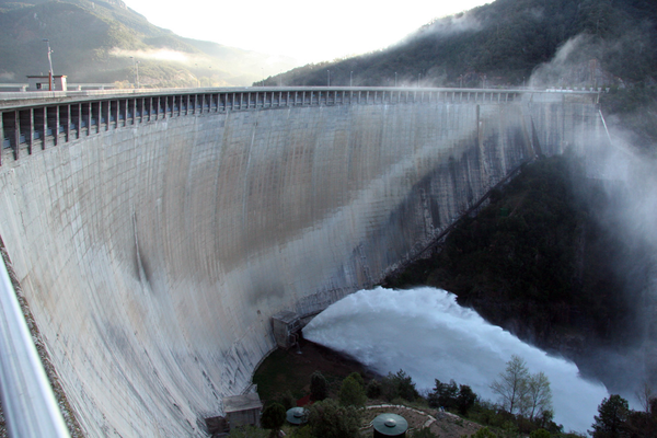
Figure 24: View of La Baells dam.

(¹) http://www.bergactual.com/wp-content/uploads/2009/04/373363.jpg

5.1 Monitoring devices at La Baells Dam

Among the available records, the study focuses on 10 variables: 6 correspond to displacements measured by pendulums (radial), and four to temperature.

The location of these pendulums is shown in Figure 25. The exact position of the pendulums is detailed in Table1. The origin of the coordinate system is the sea level and the generatrix of the archs.

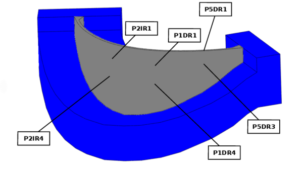
Figure 25: Position of pendulums at La Baells dam.

Table. 1 Coordinates of the pendulums at La Baells dam.

	Coordinates (m)
	X	Y	Z
P1DR1	31.60	135.10	610.00
P1DR4	31.80	136.10	590.00
P2IR1	-31.60	135.10	610.00
P2IR4	-31.80	136.10	590.00
P5DR1	90.00	101.27	628.00
P5DR3	90.40	101.80	610.00

Figure 26 shows the position of the thermometers and Table 2 provides the exact position of them.

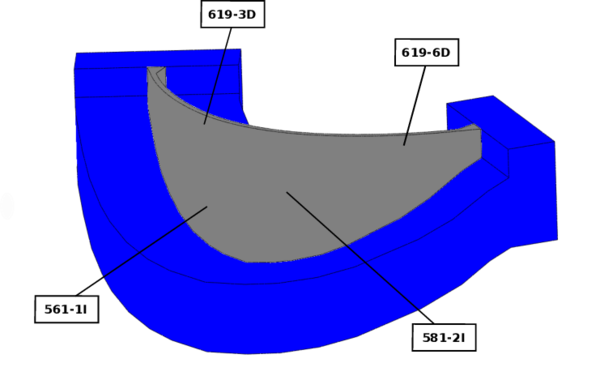
Figure 26: Position of thermometers at La Baells dam.

Table. 2 Coordinates of the thermometers at La Baells dam.

	Coordinates (m)
	X	Y	Z
619-6D	-105.95	90.03	619.00
619-3D	60.62	120.76	619.00
581-2I	-28.78	140.87	581.00
561-1I	45.72	130.57	561.00

5.2 The Problem's Data

The analysis is performed from 1994 until 2007. The information of the water level and the air mean temperature during these years are shown in Figure 27 and 28, respectively.

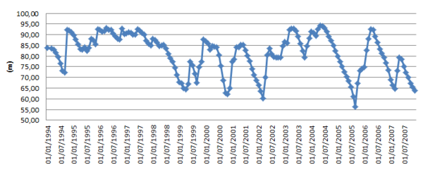
Figure 27: Hydrostatic load evolution 1994-2007.

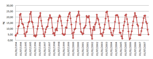
Figure 28: Air temperature evolution 1994-2007.

The problem is solved in the following way. Firstly, the thermal problem according with prescribed boundary conditions (Bofang and the air temperature) is solved. The used time step for solving the thermal problem is ${\textstyle \Delta T=1}$ month. Then, the mechanical problem taking into account the contributions of the thermal problem is solved.

Due to the thermal effects play an important role in the problem it is considered appropriate to start the resolution of the thermal problem in 1990 with the aim of obtaining a more realistic temperature field.

In all the simulations two different materials were used, concrete in the body dam, and foundation in the base. The material specifications are detailed in Table 3

Table. 3 Material properties.

Property	Concrete	Foundation
Density ${\displaystyle (kg/m^{3})}$	2,400	3,000
Specific heat ${\displaystyle (J/(kg\cdot k))}$	982	950
Conductivity ${\displaystyle (W/(m\cdot K))}$	2.43	2.2
Young Modulus ${\displaystyle (N/m^{2})}$	4.67e10	3.1e10
Poisson	0.25	0.25
Thermal expansion ${\displaystyle ^{\circ }C^{-1}}$	1e-05	1e-05

To simplify the input parameters, it was decided to compute the Bofang parameters for the period of study. To do that, a monthly mean during the study time is computed. Once the monthly mean is obtained, the input parameters to apply the formulation are computed. In Table 4, the monthly mean values of air temperature during 1994-2007 are shown.

Table. 4 Monthly mean temperature during 1994-2007.

Month	Temperature ${\displaystyle ^{\circ }C}$
January	4.27
February	5.22
March	7.22
April	10.42
May	13.00
June	18.27
July	21.50
August	21.92
September	19.13
October	15.60
November	10.82
December	5.38

The input parameters for this period of study are

${\displaystyle T_{s}=14.72\qquad T_{b}=4.96\qquad A_{0}=8.83}$

Two different Dirichlet boundary conditions need to be applied on the upstream dam face. The first condition that is applied is Bofang at the wet wall, but when the reservoir is not totally full, it is necessary to assign a value at the dry area. In this case, this temperature has been approximated adding 2 ${\textstyle ^{\circ }C}$ to the air temperature.

Downstream is also necessary to assign a temperature value. There is a vast literature about how to compute these values [2]. The used approximation was to add 2 ${\textstyle ^{\circ }C}$ to the air temperature. Another important data that must be introduced is the reference temperature. It is considered appropriate to set this value as the joints injection temperature, ${\textstyle T_{ref}=10^{\circ }C}$.

Figure 29 shows a scheme with all thermal and mechanical conditions.

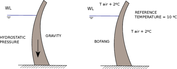
Figure 29: Thermal and mechanical boundary conditions on the dam body

A study of convergence at some points of the dam has been performed. Figure 30, shows the convergence analysis at four pendulums after solving the mechanical problem (gravity and water level equal to 93m). The study compares the obtained results using different tetrahedral meshes with the obtained values with an hexahedral mesh of 27 nodes.

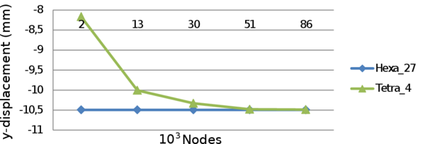
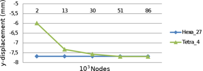
(a) P1DR1	(b) P1DR4
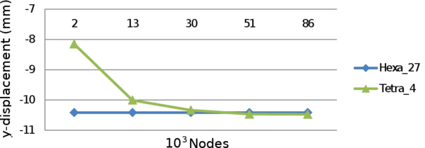
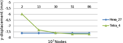
(c) P2IR1	(d) P2IR4
Figure 30: Convergence analysis at La Baells dam

A mesh of 86,000 nodes is used (Figure 31), although the mesh has converged before arriving to 86,000 nodes, the interest problem is a thermo-mechanical one and this problem is more restrictive with the element size in convergence criteria. The mesh is composed by 86,993 nodes and 323,955 tetrahedrons.

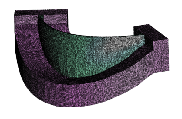
Figure 31: Tetrahedral mesh.

The contact between both volumes (dam and foundation) is carried out just by sharing nodes.

5.3 Temperature Analysis

The temperature analysis was performed using the information provided by the four thermometers previously presented. Figure 32 shows the comparison of temperatures during 2007 year between real data and the values obtained by Dam Application.

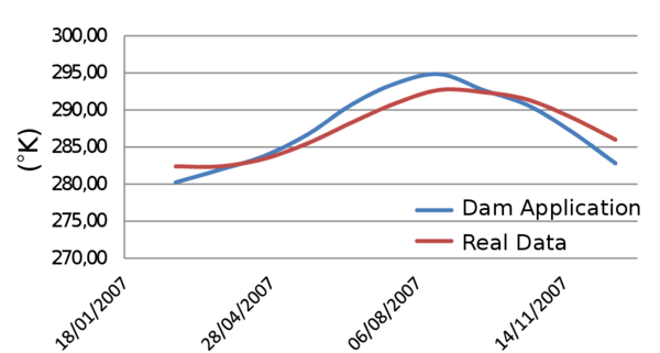
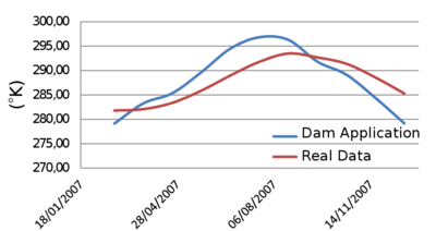
(a) 619-6D	(b) 619-3D
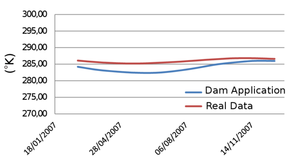
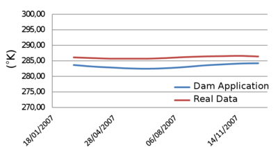
(c) 581-2I	(d) 561-1I
Figure 32: Temperature analysis at La Baells dam

Figures 32a and 32b show the evolution of temperature during 2007 in the higher parts of the dam. The temperature variation in these thermometers between winter and summer is quite high due to its position. As was commented in Chapter 4, upper positions are highly influenced by climatic conditions. The opposite occurs in thermometers 581-2I and 561-1I shown in Figure 32c and 32d, respectively. In these parts the variation is quite low.

In general terms, the temperature field is well approximated by the used formulation, the greatest differences are located in summer months.

5.4 Displacement Analysis

The displacement measurement is provided by the six pendulums previously presented. Dam displacements are measured in local axes: tangent and perpendicular to the dam axis at each location. They are termed "tangential" and "radial" displacements, respectively. In this work the radial displacements were considered, since their magnitude is greater and thus the effect of the measurement error is lower.

Since the numerical model results are provided in global Cartesian axes, they need to be rotated to be compared to the observed values. The angle of this rotation depends on the location of each pendulum. Moreover, the results suggest that some discrepancies might exist between the theoretical and the actual position of some local axes, as shown below.

Finally, a constant value was added to each radial displacement to account the displacement previous to the installation of the measurement device.

Taking all above mentioned into account the transformation of the displacement field is performed according the next formulation:

${\displaystyle u_{\theta }=u_{x}sin(\theta )+u_{y}cos(\theta )+u_{0}}$

(66)

In this work two different ways to compute the ${\textstyle \theta }$ angle are presented. The first approach to compute the ${\textstyle \theta }$ angle is to get this parameter using geometric relations provided by the model. The second approach consists in the minimization of the error, the idea is to find the angle that offers the best approximation.

Figures 33 and 34 show the ${\textstyle x-displacement}$ and ${\textstyle y-displacement}$ field in December of 2007.

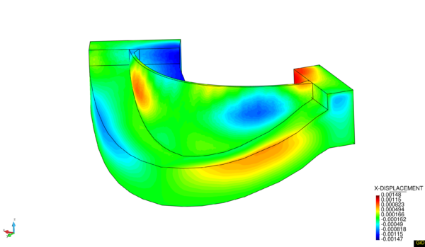
Figure 33: x-displacement field, 2007-12

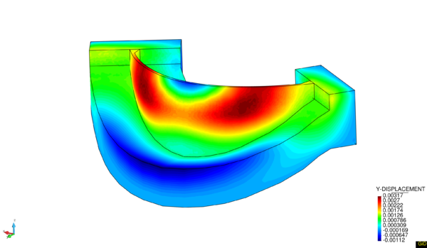
Figure 34: y-displacement field, 2007-12

Next the obtained results using each approach at each pendulum are presented.

Figure 35: Radial displacement at P1DR1 pendulum.

Figure 36: Radial displacement at P1DR4 pendulum.

Figure 37: Radial displacement at P2IR1 pendulum.

Figure 38: Radial displacement at P2IR4 pendulum.

Figure 39: Radial displacement at P5DR1 pendulum.

Figure 40: Radial displacement at P5DR3 pendulum.

Table 5 provides a summary of the angles at each pendulum according to each approach.

Table. 5 ${\displaystyle \theta }$ values for each approach.

Id	Geometric ${\displaystyle \theta }$	Optimized ${\displaystyle \theta }$
P1DR1	-13	-41
P1DR4	-16	-38
P2IR1	13	39
P2IR4	16	36
P5DR1	-35	-34
P5DR3	-39	-41

The obtained values using a geometric value of ${\textstyle \theta }$ provides accurate results, concentrating the error at peaks.

In the second approach, the optimization process, the behaviour of dam is captured more accurately. The obtained ${\textstyle \theta }$ values at the central pendulums keep the symmetry between them, and provide good results although the value is higher than geometric values. The obtained ${\textstyle \theta }$ values at the exterior pendulums (close to the abutments) have similar value than geometric ones.

In Table 6 the error depending the used approach is shown. Two different types of errors have been performed, the first one, the mean absolute error which is computed as

${\displaystyle e_{abs}={\frac {\sum _{i=1}^{n=168}\left|u_{real}-u_{computed}\right|}{168}}}$

(67)

and the mean relative error which is computed as

${\displaystyle e_{rel}={\frac {e_{abs}}{max(u_{(i)})-min(u_{(i)})}}*100}$

(68)

First approach provides an average error of ${\textstyle 8\%}$ while the second approach just a ${\textstyle 5\%}$ of error.

Table. 6 Mean absolute and mean relative error at each pendulum.

	Geometric ${\displaystyle \theta }$		Optimized ${\displaystyle \theta }$
	Abs. Er. (mm)	Rel. Er. (${\textstyle \%}$)	Abs. Er. (mm)	Rel. Er. (${\textstyle \%}$)
P1DR1	2.19	11.5	0.90	4.8
P1DR4	1.21	8.7	0.65	4.6
P2IR1	2.31	11.4	1.28	6.3
P2IR4	1.37	9.3	0.96	6.6
P5DR1	0.77	5.4	0.76	5.4
P5DR3	0.39	4.8	0.37	4.6
Average	1.38	8.5	0.82	5.4

The provided results by ${\textstyle DamApp}$ as well as the performed transformation to radial displacements approximate accurately the real data provided by the pendulums. The obtained ${\textstyle \theta }$ values in the second approach have coherence, keep the symmetry, and the numeric value is totally reasonable taking into account that pendulums can suffer distortions by different factors. The proposed numerical model captures the real behaviour of the dam accurately.

5.5 Tetrahedrons Vs Hexahedrons

In this section a comparison between the obtained results using the ${\textstyle DamApp}$ with a tetrahedral mesh and the results obtained using COMET with hexahedrons of 20 nodes (provided by M.Sc. Fernando Salazar) was performed. The aim of this study is to prove that the use of tetrahedral elements can also lead to accurate solutions.

The boundary conditions applied in Software COMET are: a constant temperature value (provided by Bofang formulation at the middle point in the wall) at upstream dam face below water level, the air temperature + 2 ${\textstyle ^{\circ }C}$ at downstream and the reference temperature equal to ${\textstyle T_{ref}=10^{\circ }C}$.

The comparison was performed using the second approach for both cases; COMET and ${\textstyle DamApp}$. Figures 41 and 42 provide the comparison through the radial displacement field at each pendulum.

(a) P1DR1	(b) P1DR4
(c) P2IR1	(d) P2IR4
Figure 41: Radial displacement comparison at central pendulums

(a) P5DR1	(b) P5DR3
Figure 42: Radial displacement comparison at exterior pendulums

Table 7 shows the obtained results through the mean absolute error for both approaches.

Table. 7 Mean absolute error at each pendulum (mm).

	Geometric ${\displaystyle \theta }$		Optimized ${\displaystyle \theta }$
	Dam App	COMET	Dam App	COMET
P1DR1	2.19	1.19	0.90	0.96
P1DR4	1.21	0.64	0.65	0.60
P2IR1	2.31	1.44	1.28	1.28
P2IR4	1.37	0.97	0.96	0.95
P5DR1	0.77	1.56	0.76	0.62
P5DR3	0.39	0.89	0.37	0.70
Average	1.37	1.12	0.82	0.85

Same comparison but this time through the mean relative error is shown in Table 8.

Table. 8 Mean relative error at each pendulum (${\displaystyle \%}$).

	Geometric ${\displaystyle \theta }$		Optimized ${\displaystyle \theta }$
	Dam App	COMET	Dam App	COMET
P1DR1	11.5	6.2	4.8	5.1
P1DR4	8.7	4.6	4.6	4.3
P2IR1	11.4	7.1	6.3	6.3
P2IR4	9.3	6.6	6.6	6.5
P5DR1	5.4	10.9	5.4	4.4
P5DR3	4.8	10.9	4.6	8.6
Average	8.5	7.7	5.4	5.9

According with the obtained results (Table 7 and 8) the use of tetrahedral elements leads to accurate solutions. These results also prove the correct working of the new Application (${\textstyle DamApp}$).

6 Conclusions

This thesis presents a new application inside the KRATOS environment for elastic structural verification of dams.

The thermo-mechanical coupling was solved by introducing a thermal component into the mechanical constitutive law (one way coupling), and based on the obtained results, this modified equation is able to approach the physics of the real problem.

The developed graphical interface satisfies the basic user’s requirements. The application has a user friendly design and offers the possibility of self-customization through the use of input data tables.

Regarding the new implemented boundary conditions, the Bofang constrain provides an accurate temperature field in the upstream submerged part and its annual variation is in good agreement with the test field measurements. The limited range of temperatures given in the cases analysed, permits simplifying the application of the Bofang law. The uplift condition was implemented without taking into account the influence of drains.

On the other hand, with this thesis it was proved that the use of tetrahedral elements can be a valid option for these type of simulations. In dam engineering, the use of hexahedral elements in numerical analysis is very common due to its good response under bending loads. However, hexahedral elements become too rigid when it is required to deal with non-regular geometries, e.g. when taking into account the influence of a spillway. For a complex geometry, the use of tetrahedral elements presents a good option. Regarding the computational cost, the hexahedrons is expensive compared to the tetrahedrons.

As a final conclusion, the software Dam Application (DamApp) satisfies all the requested objectives, providing accurate results within a user-friendly interface.

As a future works, some improvements can be implemented in order to improve the robustness of this application:

• Interface: the new should be based on a tree interface architecture. This change will improve the accessibility to the different options and will increment the flexibility of the software.
• Joint Elements: in dams engineering these special elements play an important role. As a main feature, they can capture the jumps in displacement, stress and strain fields. Its presence reduces the elastic and strength properties of materials and introduces directional preferences [28].
• Drains: if included, it will provide a more realistic approach for computing the uplift pressure. Then, the influence of the drain position will be considered, which is crucial to determine traction and compressive areas in the base of the dam.

As long term goal, it can be mentioned: the development of a module for simulating the solidification process during the construction phase, the introduction of non-linear constitutive laws, the coupling between fluid- structure and foundation (e.g. in a rock joint), all of them with the aim of analyzing extreme conditions.

7 Finite Element Method

This appendix is an overview of Finite Element Method (FEM) applied to the mechanical problem. Mainly, is based in the book of Prof. Eugenio Oñate, Structural Analysis with the Finite Element Method. Linear Statics [12] [13], where all these concepts are dealt extensively and in the book of Prof. Xavier Oliver and Prof. Carlos Agelet de Saracibar, Mecánica de medios continuos para ingenieros [14].

7.1 Two Dimensional Elasticity Theory

7.1.1 Introduction

There are a wide number of structures of practical interest which can be analysed following the assumptions of 2D elasticity. These types of structure have a sort of prismatic geometry. Depending on the relative dimensions of the prism and the loading type, two categories can be distinguished;

• Plane Stress problems. A prismatic structure is under plane stress if one of its dimensions (thickness) is much smaller than the other two and all loads are contained in the middle plane of the structure. The analysis domain is the middle section (Figure 43).

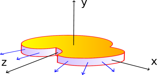
Figure 43: Plate under plane stress

• Plane Strain problems. A prismatic structure is under plane strain if one of its dimensions (length) is larger than the other two and all the loads are uniformly distributed along its length and they act orthogonally to the longitudinal axis. The analysis domain is a cross section to this axis (Figure 44).

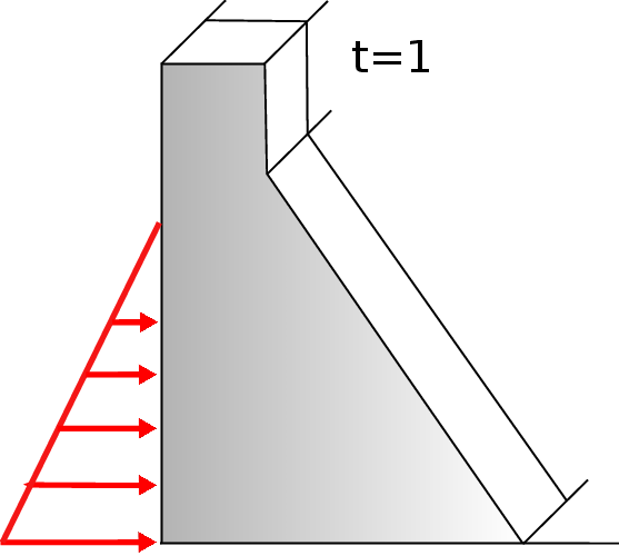
Figure 44: Section under plane strain

7.1.2 Concepts

Displacements, strains and stresses fields

Plane stress and plane strain assumptions imply that transversal sections to the prismatic ${\textstyle z-axis}$ deform in the same way, and the displacement along z axis is also negligible. Applying this simplification only a generic 2D transverse section in the plane ${\textstyle x-y}$ needs to be considered for the analysis. The displacement vector field of a point is

${\displaystyle {\textbf {u}}(x,y)=\left\{{\begin{matrix}u(x,y)\\v(x,y)\end{matrix}}\right\}}$

(69)

Strains can be derived by the displacement field 69

${\displaystyle \varepsilon _{x}={\frac {\partial u}{\partial x}},\qquad \varepsilon _{y}={\frac {\partial v}{\partial y}}\qquad \gamma _{xy}={\frac {\partial u}{\partial y}}+{\frac {\partial v}{\partial x}},\qquad \gamma _{xz}=\gamma _{yz}=0}$

(70)

In plane strain case, the longitudinal strain (${\textstyle \varepsilon _{z}}$) is assumed to be zero, but not for plane stress problem where ${\textstyle \sigma _{z}}$ is considered zero. The strain vector can be described as

${\displaystyle {\boldsymbol {\varepsilon }}=[\varepsilon _{x},\varepsilon _{y},\gamma _{xy}]^{T}}$

(71)

From the equations of the strain field 70 is deduced that ${\textstyle \tau _{xz}}$ and ${\textstyle \tau _{yz}}$ are zero. As it was explained, the longitudinal stress (${\textstyle \sigma _{z}}$) does not contribute to the internal work. The stress vector can be described as

${\displaystyle {\boldsymbol {\sigma }}=[\sigma _{x},\sigma _{y},\tau _{xy}]^{T}}$

(72)

According with 3D elasticity theory and applying the stated assumptions, the following matrix relationship can be obtained

${\displaystyle {\boldsymbol {\sigma }}={\textbf {C}}\;{\boldsymbol {\varepsilon }}}$

(73)

where C is the elastic material matrix or constitutive matrix

${\displaystyle {\textbf {C}}={\begin{bmatrix}c_{11}&c_{12}&0\\c_{21}&c_{22}&0\\0&0&c_{33}\end{bmatrix}}}$

(74)

Depending on the type of problem, the components of matrix ${\textstyle {\textbf {C}}}$ take different expression. An usual way to define these coefficients is as function of ${\textstyle E}$ Young Modulus and ${\textstyle \nu }$ Poisson's ratio. According with Maxwell-Betti theorem, ${\textstyle {\textbf {C}}}$ is always symmetrical, so ${\textstyle c_{12}=c_{21}}$.

In the case of isotropic elasticity, the components of ${\textstyle {\textbf {C}}}$ 74 are

${\displaystyle {\begin{array}{c}Plane\;Stress\\\displaystyle c_{11}=c_{22}={\frac {E}{(1-\nu ^{2})}}\\c_{12}=c_{21}=\nu d_{11}\\\displaystyle c_{33}={\frac {E}{2(1+\nu )}}=G\end{array}}\qquad \qquad {\begin{array}{c}Plane\;Strain\\\displaystyle c_{11}=c_{22}={\frac {E(1-\nu )}{(1+\nu )(1-2\nu )}}\\\displaystyle c_{12}=c_{21}={\frac {\nu }{1-\nu }}d_{11}\\\displaystyle c_{33}={\frac {E}{2(1+\nu )}}=G\end{array}}}$

(75)

For an orthotropic material with principal orthotropy directions along the 1, 2, 3 axis (where 3 is out-of-plane direction), the matrix ${\textstyle {\textbf {C}}}$ takes the following expression for plane stress and plane strain, respectively.

${\displaystyle {\textbf {C}}={\frac {1}{1-\nu _{12}\nu _{21}}}{\begin{bmatrix}E_{1}&\nu _{21}E_{1}&0\\\nu _{12}E_{2}&E_{2}&0\\0&0&(1-\nu _{12}\nu _{21})G_{12}\end{bmatrix}}}$

(76)

${\displaystyle {\textbf {C}}={\frac {1}{ad-bc}}{\begin{bmatrix}aE_{1}&bE_{1}&0\\cE_{2}&dE_{2}&0\\0&0&(ad-bc)G_{12}\end{bmatrix}}}$

(77)

where

${\displaystyle {\frac {1}{G_{12}}}\simeq {\frac {1+\nu _{21}}{E_{1}}}+{\frac {1+\nu _{12}}{E_{2}}}}$

${\displaystyle a=1-\nu _{23}\nu _{32};\qquad b=\nu _{12}+\nu _{32}\nu _{13}}$ ${\displaystyle c=\nu _{21}+\nu _{23}\nu _{31};\qquad d=1-\nu _{13}\nu _{31}}$

The symmetry of ${\textstyle {\textbf {C}}}$ requires (Maxwell-Betti Theorem)

${\displaystyle {\begin{array}{c}Plane\;Stress\\\displaystyle {\frac {E_{1}}{E_{2}}}={\frac {\nu _{12}}{\nu _{21}}}\end{array}}\qquad {\begin{array}{c}Plane\;Strain\\\displaystyle {\frac {E_{1}}{E_{2}}}={\frac {c}{b}}\end{array}}}$

(78)

In the case that the solid is subjected to initial stress, the constitutive relationship must be modified. The total strain (${\textstyle {\boldsymbol {\varepsilon }}}$) can be divided as the sum of elastic (${\textstyle {\boldsymbol {\varepsilon ^{e}}}}$) and initial (${\textstyle {\boldsymbol {\varepsilon ^{0}}}}$) strains. The constitutive equation reads as

${\displaystyle {\boldsymbol {\sigma }}={\textbf {C}}\;{\boldsymbol {\varepsilon }}={\textbf {C}}({\boldsymbol {\varepsilon ^{e}}}-{\boldsymbol {\varepsilon ^{0}}})}$

(79)

Thermal strain contributions

One of the possible causes of initial strains 79 is the thermal effect. In the case of isotropic material, the expression of the vector can read as

${\displaystyle {\begin{array}{c}Plane\;Stress\\{\boldsymbol {\varepsilon ^{0}}}=\left\lbrace {\begin{array}{lll}\alpha \Delta T\\\alpha \Delta T\\0\end{array}}\right\rbrace \end{array}}\qquad {\begin{array}{c}Plane\;Strain\\{\boldsymbol {\varepsilon ^{0}}}=(1+\nu )\left\lbrace {\begin{array}{lll}\alpha \Delta T\\\alpha \Delta T\\0\end{array}}\right\rbrace \end{array}}}$

(80)

where ${\textstyle \alpha }$ is the thermal expansion coefficient and ${\textstyle \Delta }$T is the temperature variation at each point. As it is shown in the thermal strain vector, the temperature variation does not generate shear strains.

Initial stresses

The solid can also be subjected to initial stress (${\textstyle {\boldsymbol {\sigma ^{0}}}}$). This initial stress can come from different sources. The total stress in the new equilibrium configuration is just the addition of initial stress to the Eq.79

${\displaystyle {\boldsymbol {\sigma }}={\textbf {C}}({\boldsymbol {\varepsilon ^{e}}}-{\boldsymbol {\varepsilon ^{0}}})+{\boldsymbol {\sigma ^{0}}}}$

(81)

where ${\textstyle {\boldsymbol {\sigma ^{0}}}}$ can be decomposed as

${\displaystyle {\boldsymbol {\sigma ^{0}}}=[\sigma _{x}^{0},\sigma _{y}^{0},\tau _{xy}^{0}]^{T}}$

(82)

Virtual work expression

The Principle of Virtual Work (PVW) for 2D elasticity problem can be stated as [29]

${\displaystyle \iint _{A}(\delta \varepsilon _{x}\sigma _{x}+\delta \varepsilon _{y}\sigma _{y}+\delta \gamma _{xy}\tau _{xy})t\;dA=\iint _{A}(\delta ub_{x}+\delta vb_{y})t\;dA+}$ ${\displaystyle \oint _{l}(\delta ut_{x}+\delta vt_{y})t\;ds+\sum _{i}(\delta u_{i}P_{x_{i}}+\delta v_{i}P_{y_{i}})}$

(83)

The integral in the l.h.s represents the work performed by the stresses (${\textstyle \sigma _{x}}$, ${\textstyle \sigma _{y}}$, ${\textstyle \tau _{xy}}$) over the virtual strains (${\textstyle \delta \varepsilon _{x}}$, ${\textstyle \delta \varepsilon _{y}}$, ${\textstyle \delta \gamma _{xy}}$). The terms in r.h.s represent the virtual work of the body forces (${\textstyle b_{x}}$, ${\textstyle b_{y}}$); the surface tractions (${\textstyle t_{x}}$, ${\textstyle t_{y}}$); and the external points loads (${\textstyle P_{xi}}$, ${\textstyle P_{yi}}$). ${\textstyle A}$ is the area and ${\textstyle l}$ is the boundary of the transverse section. For a plane stress problem ${\textstyle t}$ is the thickness of the solid, and for plane strain problem ${\textstyle t}$ is equal to one.

The PVW shows us the continuity requirements. Derivatives of the displacements are needed, so ${\textstyle C^{0}}$ continuity is needed.

7.1.3 Natural coordinates and shape functions

The shape function is a fundamental concept to understand the Finite Element Method (FEM). Shape functions (${\textstyle N}$) are defined at each node of a finite element, and allow us to obtain the value of a nodal variable at any point of the element through interpolation.

Before introducing the shape functions of the linear triangular elements and the four-noded Lagrangian elements, the concept of natural coordinates is presented.

The natural coordinates (${\textstyle \xi }$, ${\textstyle \eta }$) are normalized coordinates (range from -1 to 1). From Figure 45 can be deduced that

${\displaystyle \xi ={\frac {x-x_{c}}{a}}\qquad ;\qquad \eta ={\frac {y-y_{c}}{b}}}$

(84)

${\displaystyle {\frac {d\xi }{dx}}={\frac {1}{a}}\qquad ;\qquad {\frac {d\eta }{dy}}={\frac {1}{b}}}$

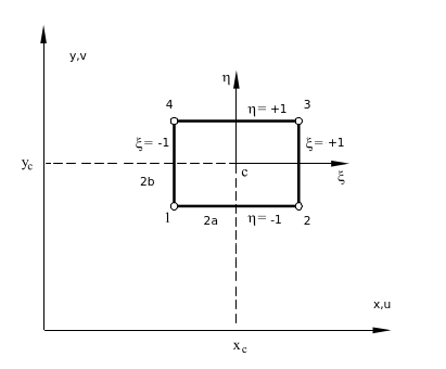
Figure 45: Natural coordinate system for rectangular element

where ${\textstyle x_{c}}$ and ${\textstyle y_{c}}$ are the coordinates of the element centroid. The differentials of area in Cartesian and natural systems are related by

${\displaystyle dx\;dy=ab\;d\xi \;d\eta }$

(85)

The integration of a function (${\textstyle f(x,y)}$) over a rectangular element can be expressed in natural system as

${\displaystyle \iint _{A^{(e)}}f(x,y)dx\;dy=\int _{-1}^{+1}\int _{-1}^{+1}g(\xi ,\eta )ab\;d\xi \;d\eta }$

(86)

The shape functions can only reproduce exactly a polynomial solution of order equal or less than a polynomial contained in the shape functions. Pascal's triangle (Figure 46) shows the relation between the polynomial degree and the number of needed terms. It can be deduced that the higher is the order of that complete polynomial, the more accurate is the finite element solution.

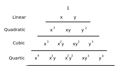
Figure 46: Pascal's triangle in two dimensions

A 2D complete polynomial of ${\textstyle nth}$ degree can be written as

${\displaystyle f(x,y)=\sum _{i=1}^{p}\alpha _{i}x^{j}y^{k}\qquad j+k\leq n}$

(87)

where the number of terms is

${\displaystyle p=(n+1)(n+2)/2}$

(88)

The shape functions of triangles and tetrahedrons are formed by complete polynomials, but quadrilaterals and hexahedrons contain incomplete polynomial terms.

Shape functions must satisfy the same requirements in natural coordinates and in Cartesian coordinates. These conditions are:

• Condition of nodal compatibility

${\displaystyle N_{i}(\xi _{j},\eta _{j})={\begin{array}{ll}1\qquad i=j\\0\qquad i\neq j\end{array}}}$

(89)

• Rigid body motion

${\displaystyle \sum _{i=1}^{n}N_{i}(\xi ,\eta )=1}$

(90)

Only two basic types of elements are presented: the triangular element of three nodes [30] and the rectangular Lagrangian element of four nodes.

The four-noded Lagrangian element (Figure 47) is the simplest element of the Lagrangian family and it coincides with the element developed by Argyris and Kelsey [31]. The way to obtain the shape functions is presented hereafter. Considering a generic node ${\textstyle i}$, the 1D shape functions in local directions (${\textstyle \xi }$,${\textstyle \eta }$) can be expressed as

${\displaystyle l_{1}^{i}(\xi )={\frac {1}{2}}(1+\xi \xi _{i})\qquad ;\qquad l_{1}^{i}(\eta )={\frac {1}{2}}(1+\eta \eta _{i})}$

(91)

In this case, values of ${\textstyle I}$ and ${\textstyle J}$ take a value equal to 1 since is a linear element. To obtain the shape functions for a 4-noded Lagrangian element only is necessary to multiply together, obtaining

${\displaystyle N_{i}(\xi ,\eta )=l_{1}^{i}(\xi )l_{1}^{i}(\eta )={\frac {1}{4}}(1+\xi \xi _{i})(1+\eta \eta _{i})}$

(92)

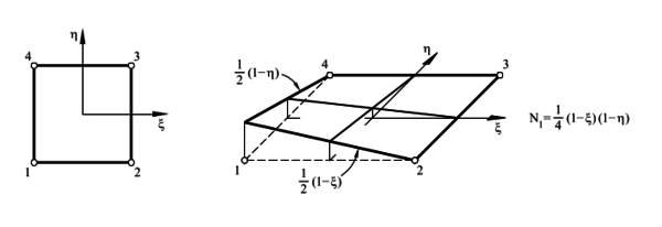
Figure 47: Four-noded Lagrangian element

The shape functions of the linear triangular element in natural coordinates (Figure 48) are presented below

${\displaystyle N_{1}=1-\xi -\eta ;\qquad N_{2}=\xi ;\qquad N_{3}=\eta }$

(93)

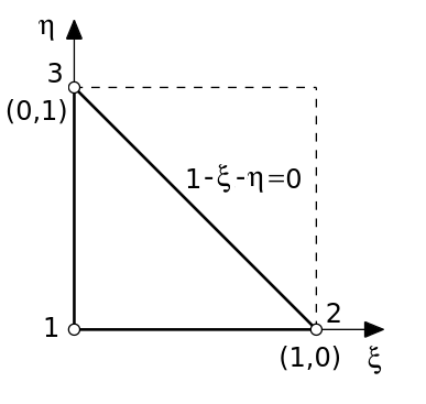
Figure 48: Natural coordinates for a triangular linear element

7.1.4 Discretization of the displacements, strains and stresses fields

For a generic two-dimensional element of ${\textstyle n}$ nodes, the displacement field can be defined as

${\displaystyle u=\sum _{i=1}^{n}N_{i}u_{i};\qquad v=\sum _{i=1}^{n}N_{i}v_{i};}$

(94)

where ${\textstyle u_{i}}$, ${\textstyle v_{i}}$ are the horizontal and vertical displacements and ${\textstyle N_{i}}$ is the shape function of node ${\textstyle i}$. In matrix form can be rewritten as

${\displaystyle {\textbf {u}}={\begin{bmatrix}u\\v\end{bmatrix}}={\begin{bmatrix}N_{1}&0&\cdots &N_{n}&0\\0&N_{1}&\cdots &0&N_{n}\end{bmatrix}}{\begin{bmatrix}u_{1}\\v_{1}\\\vdots \\u_{n}\\v_{n}\end{bmatrix}}}$

(95)

or

${\displaystyle {\textbf {u}}={\textbf {N}}{\textbf {a}}^{(e)}}$

(96)

where u is the displacement vector of a point. The shape functions matrix of the element and the ${\textstyle i}$th node are defined as

${\displaystyle {\textbf {N}}=[{\textbf {N}}_{1},{\textbf {N}}_{2},\cdots ,{\textbf {N}}_{n}];\qquad {\textbf {N}}_{i}={\begin{bmatrix}{\textbf {N}}_{i}&0\\0&{\textbf {N}}_{i}\end{bmatrix}}}$

(97)

The nodal displacement vector of the element and the ${\textstyle i}$th node are defined as

${\displaystyle {\textbf {a}}^{(e)}={\begin{bmatrix}{\textbf {a}}_{1}^{(e)}\\{\textbf {a}}_{2}^{(e)}\\\vdots \\{\textbf {a}}_{n}^{(e)}\end{bmatrix}}\qquad with\qquad {\textbf {a}}_{i}^{(e)}={\begin{bmatrix}u_{i}\\v_{i}\end{bmatrix}}}$

(98)

In the case of the strain field, it can be written as

${\displaystyle \varepsilon _{x}={\frac {\partial u}{\partial x}}=\sum _{i=1}^{n}{\frac {\partial N_{i}}{\partial x}}u_{i}}$

${\displaystyle \varepsilon _{y}={\frac {\partial v}{\partial y}}=\sum _{i=1}^{n}{\frac {\partial N_{i}}{\partial y}}v_{i}}$

(99)

${\displaystyle \gamma _{xy}={\frac {\partial u}{\partial y}}+{\frac {\partial v}{\partial x}}=\sum _{i=1}^{n}({\frac {\partial N_{i}}{\partial y}}u_{i}+{\frac {\partial N_{i}}{\partial x}}v_{i})}$

which in matrix form is written as

${\displaystyle {\boldsymbol {\varepsilon }}={\begin{bmatrix}{\frac {\partial u}{\partial x}}\\{\frac {\partial v}{\partial y}}\\{\frac {\partial u}{\partial y}}+{\frac {\partial v}{\partial x}}\end{bmatrix}}={\begin{bmatrix}{\frac {\partial N_{1}}{\partial x}}&0&\cdots &{\frac {\partial N_{n}}{\partial x}}&0\\0&{\frac {\partial N_{1}}{\partial y}}&\cdots &0&{\frac {\partial N_{n}}{\partial y}}\\{\frac {\partial N_{1}}{\partial y}}&{\frac {\partial N_{1}}{\partial x}}&\cdots &{\frac {\partial N_{n}}{\partial y}}&{\frac {\partial N_{n}}{\partial x}}\end{bmatrix}}{\begin{bmatrix}u_{1}\\v_{1}\\\vdots \\u_{n}\\v_{n}\end{bmatrix}}}$

(100)

or

${\displaystyle {\boldsymbol {\varepsilon }}={\textbf {B}}{\textbf {a}}^{(e)}}$

(101)

where

${\displaystyle {\textbf {B}}=[{\textbf {B}}_{1},{\textbf {B}}_{2},\cdots ,{\textbf {B}}_{n}]}$

(102)

is the element strain matrix and

${\displaystyle {\textbf {B}}_{i}={\begin{bmatrix}\displaystyle {\frac {\partial N_{i}}{\partial x}}&0\\0&\displaystyle {\frac {\partial N_{i}}{\partial y}}\\{\frac {\partial N_{i}}{\partial y}}&\displaystyle {\frac {\partial N_{i}}{\partial x}}\end{bmatrix}}}$

(103)

is the strain matrix of node ${\textstyle i}$.

To obtain the expression of the stresses field, it is just needed the substitution of Eq.101 into Eq.73, obtaining

${\displaystyle {\boldsymbol {\sigma }}={\textbf {C}}{\boldsymbol {\varepsilon }}={\textbf {C}}{\textbf {B}}{\textbf {a}}^{(e)}}$

(104)

If initial strains and stresses are considered, from Eq.81 can be deduced that

${\displaystyle {\boldsymbol {\sigma }}={\textbf {C}}({\boldsymbol {\varepsilon }}-{\boldsymbol {\varepsilon }}^{0})+{\boldsymbol {\sigma }}^{0}={\textbf {C}}{\textbf {B}}{\textbf {a}}^{(e)}-{\textbf {B}}{\boldsymbol {\varepsilon }}^{0}+{\boldsymbol {\sigma }}^{0}}$

(105)

7.1.5 Discretized equilibrium equations

From the Principle of Virtual Works expression applied at the equilibrium of an element is possible to obtain the expressions of the stiffness matrix K and the force vector f.

Let us suppose that the uniformly distributed forces per unit area act over the body of the element (mass forces b), and uniformly distributed forces per unit length act over one of its sides (surface forces t). Moreover, supposing that the equilibrium of the element is achieved at the nodes, it is possible to define punctual forces acting at the nodes (nodal forces of equilibrium q) that must balance the forces that appear due to the element deformation and the rest of applied forces.

Taking into account these assumptions and using Eq.83, the Principle of Virtual Works applied to the element is written as

${\displaystyle \iint _{A^{(e)}}\delta {\boldsymbol {\varepsilon ^{T}}}{\boldsymbol {\sigma }}\;t\;dA=\iint _{A^{(e)}}\delta {\textbf {u}}^{T}{\textbf {b}}\;t\;dA+\oint _{l^{(e)}}\delta {\textbf {u}}^{T}{\textbf {t}}\;t\;ds+[\delta {\textbf {a}}^{(e)}]^{T}{\textbf {q}}^{(e)}}$

(106)

In plane stress problems, ${\textstyle t}$ is the real thickness of the structure, while in plane strain ${\textstyle t}$ usually takes the value of 1.

From Eq.96 and Eq.101, it is possible to write

${\displaystyle \delta {\textbf {u}}^{T}=[\delta {\textbf {a}}^{(e)}]^{T}{\textbf {N}}^{T}\qquad ;\qquad \delta {\boldsymbol {\varepsilon ^{T}}}=[\delta {\textbf {a}}^{(e)}]^{T}{\textbf {B}}^{T}}$

(107)

Substituting these equations in Eq.106, the next expression is obtained

${\displaystyle [\delta {\textbf {a}}^{(e)}]^{T}\left[\iint _{A^{(e)}}{\textbf {B}}^{T}{\boldsymbol {\sigma }}\;t\;dA-\iint _{A^{(e)}}{\textbf {N}}^{T}{\boldsymbol {b}}\;t\;dA-\oint _{l^{(e)}}{\textbf {N}}^{T}{\textbf {t}}\;t\;ds\right]=[\delta {\textbf {a}}^{(e)}]^{T}{\textbf {q}}^{(e)}}$

(108)

Due to the arbitrariness of the virtual displacements ${\textstyle [\delta {\textbf {a}}^{(e)}]^{T}}$, the expression can be written as

${\displaystyle \iint _{A^{(e)}}{\textbf {B}}^{T}{\boldsymbol {\sigma }}\;t\;dA-\iint _{A^{(e)}}{\textbf {N}}^{T}{\boldsymbol {b}}\;t\;dA-\oint _{l^{(e)}}{\textbf {N}}^{T}{\textbf {t}}\;t\;ds={\textbf {q}}^{(e)}}$

(109)

Using the stress expression of Eq.105, the following expression is obtained

${\displaystyle \iint _{A^{(e)}}{\textbf {B}}^{T}({\textbf {C}}{\textbf {B}}{\textbf {a}}^{(e)}-{\textbf {C}}{\boldsymbol {\varepsilon ^{0}}}+{\boldsymbol {\sigma ^{0}}})\;t\;dA-\iint _{A^{(e)}}{\textbf {N}}^{T}{\boldsymbol {b}}\;t\;dA-\oint _{l^{(e)}}{\textbf {N}}^{T}{\textbf {t}}\;t\;ds={\textbf {q}}^{(e)}}$

(110)

after rearranging terms, the equation reads as

${\displaystyle \left[\iint _{A^{(e)}}{\textbf {B}}^{T}{\textbf {C}}{\textbf {B}}\;tdA\right]{\textbf {a}}^{(e)}-\iint _{A^{(e)}}{\textbf {B}}^{T}{\textbf {C}}{\boldsymbol {\varepsilon ^{0}}}\;tdA}$ ${\displaystyle -\iint _{A^{(e)}}{\textbf {B}}^{T}{\boldsymbol {\sigma ^{0}}}\;tdA-\iint _{A^{(e)}}{\textbf {N}}^{T}{\boldsymbol {b}}\;tdA-\oint _{l^{(e)}}{\textbf {N}}^{T}{\textbf {t}}\;tds={\textbf {q}}^{(e)}}$

(111)

it can also be expressed as

${\displaystyle {\textbf {K}}^{(e)}\;{\textbf {a}}^{(e)}-{\textbf {f}}^{(e)}\;=\;{\textbf {q}}^{(e)}}$

(112)

where

${\displaystyle {\textbf {K}}^{(e)}=\iint _{A^{(e)}}{\textbf {B}}^{T}{\textbf {C}}{\textbf {B}}\;tdA}$

(113)

is the elastic stiffness matrix of the element, and

${\displaystyle {\textbf {f}}^{(e)}={\textbf {f}}_{\varepsilon }^{(e)}+{\textbf {f}}_{\sigma }^{(e)}+{\textbf {f}}_{b}^{(e)}+{\textbf {f}}_{t}^{(e)}}$

(114)

the equivalent nodal force vector for the element, formed by initial strains, initial stresses, body forces and surface tractions. These vectors can be defined as

${\displaystyle {\textbf {f}}_{\varepsilon }^{(e)}=\iint _{A^{(e)}}{\textbf {B}}^{T}{\textbf {C}}{\boldsymbol {\varepsilon }}^{0}t\;dA}$

(115)

${\displaystyle {\textbf {f}}_{\sigma }^{(e)}=\iint _{A^{(e)}}{\textbf {B}}^{T}{\boldsymbol {\sigma }}^{0}t\;dA}$

(116)

${\displaystyle {\textbf {f}}_{b}^{(e)}=\iint _{A^{(e)}}{\textbf {N}}^{T}{\boldsymbol {b}}t\;dA}$

(117)

${\displaystyle {\textbf {f}}_{t}^{(e)}=\oint _{l^{(e)}}{\textbf {N}}^{T}{\boldsymbol {t}}t\;ds}$

(118)

The global equilibrium equation of the mesh is obtained just imposing the sum of nodal forces of equilibrium at each node must be equal to the external forces

${\displaystyle \sum _{e}={\textbf {q}}_{i}^{(e)}={\textbf {p}}_{j}}$

(119)

where the left part of the expression represents the sum of contributions of the vectors of nodal forces of equilibrium of the different elements that are sharing the global node j, and ${\textstyle {\textbf {p}}_{j}}$ represents the vector of external punctual forces acting on such node. Therefore, the global equilibrium equation of the mesh can be obtained by assembling the contributions of stiffness matrices and the equivalent nodal force vectors of each element. The global matrix equation can be written as

${\displaystyle {\textbf {K}}\;{\textbf {a}}=\;{\textbf {f}}}$

(120)

where K, a and f are respectively the stiffness matrix, the vector of nodal displacements, and the vector of equivalent nodal forces of the whole mesh.

7.2 Three Dimensional Elasticity

7.2.1 Introduction

There are structures that due to geometrical, mechanical or loading aspects are not possible to compute using plane stress, plane strain or axisymmetric assumptions. The only alternative is performing a full three dimensional (3D) analysis using the general 3D elasticity theory.

Despite its apparent complexity, the analysis of a 3D solid with FEM does not introduce major conceptual issues. 3D elasticity theory is a straightforward extension of the 2D case. Some examples of solids with irregular shapes are shown in Figure 49.

]

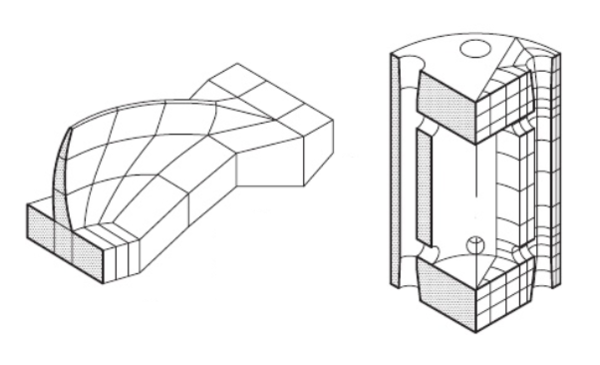Figure 49: Structures which require a 3D analysis: a) Double arch dam including foundation effects. b) Pressure vessel. Imagen taken from [12]

The structure of this section is the same as previous one.

7.2.2 Concepts

Displacements, strains and stresses fields

The displacement vector field of a point is defined by three components

${\displaystyle {\textbf {u}}=[u,v,w]^{T}}$

(121)

where ${\textstyle u}$, ${\textstyle v}$, and ${\textstyle w}$ are the displacements of a point in the direction of cartesian axes (${\textstyle x}$, ${\textstyle y}$, ${\textstyle z}$), respectively.

The strain field is defined by the six standard components of 3D elasticity [32]. The strain vector is written as

${\displaystyle {\boldsymbol {\varepsilon }}=[\varepsilon _{x},\varepsilon _{y},\varepsilon _{z},\gamma _{xy},\gamma _{xz},\gamma _{yz}]^{T}}$

(122)

The normal strain (${\textstyle \varepsilon _{z}}$) and the tangential strains (${\textstyle \gamma _{xz}}$, ${\textstyle \gamma _{yz}}$) are not equal to 0 anymore, and can be computed as

${\displaystyle \varepsilon _{z}={\frac {\partial w}{\partial z}},\qquad \gamma _{xz}={\frac {\partial u}{\partial z}}+{\frac {\partial w}{\partial x}},\qquad \gamma _{yz}={\frac {\partial v}{\partial z}}+{\frac {\partial w}{\partial y}}}$

(123)

The stress field is defined by the six stress components which are the conjugate of the six non-zero strains Eq.123. The stress vector is

${\displaystyle {\boldsymbol {\sigma }}=[\sigma _{x},\sigma _{y},\sigma _{z},\tau _{xy},\tau _{xz},\tau _{yz}]^{T}}$

(124)

According with 3D elasticity theory (Eq.73) and assuming an isotropic material, the constitutive matrix ${\textstyle {\textbf {C}}}$ reads as

${\displaystyle {\textbf {C}}={\frac {E(1-\nu )}{(1+\nu )(1-2\nu )}}{\begin{bmatrix}1&{\frac {\nu }{1-\nu }}&{\frac {\nu }{1-\nu }}&0&0&0\\&1&{\frac {\nu }{1-\nu }}&0&0&0\\&&1&0&0&0\\&Symmetrical&&{\frac {1-2\nu }{2(1-\nu )}}&0&0\\&&&&{\frac {1-2\nu }{2(1-\nu )}}&0\\&&&&&{\frac {1-2\nu }{2(1-\nu )}}\end{bmatrix}}}$

(125)

In the case of isotropic materials only are required two parameters: the Young modulus (${\textstyle E}$) and the Poisson's ratio (${\textstyle \nu }$). In the general case, anisotropic elasticity, the constitutive matrix is composed by 21 independent parameters.

Initial strains and stresses

Taking into account the contribution of initial strains and stresses, it is possible to write

${\displaystyle {\boldsymbol {\sigma }}={\textbf {C}}({\boldsymbol {\varepsilon ^{e}}}-{\boldsymbol {\varepsilon ^{0}}})+{\boldsymbol {\sigma ^{0}}}}$

(126)

Thermal strain contribution

The initial strain vector due to thermal effects can be defined as

${\displaystyle \varepsilon ^{0}=\alpha (\Delta T)[1,1,1,0,0,0]^{T}}$

(127)

Virtual work principle

The PVW expression for solids in three dimensions is

${\displaystyle \iiint _{V}\delta {\boldsymbol {\varepsilon ^{T}}}\sigma \;dV=\iiint _{V}\delta {\textbf {u}}^{T}{\textbf {b}}\;dV+\iint _{A}\delta {\textbf {u}}^{T}{\textbf {t}}\;dA+\sum _{i}\delta {\textbf {a}}_{i}^{T}{\textbf {p}}_{i}}$

(128)

Eq.128 is just an extension of 2D solids Eq.83. It is worth to remark that is written in vectorial form.

7.2.3 Natural coordinates and shape functions

Before introducing the shape functions, the formulation of natural coordinates for a 3D case is presented.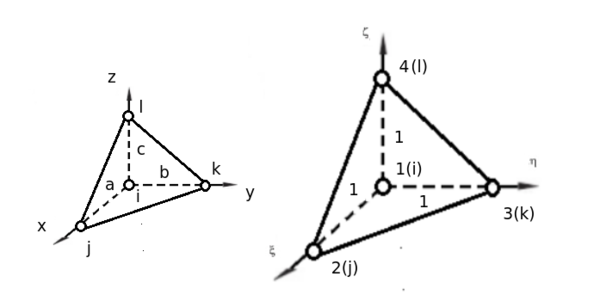

Figure 50: Natural coordinates system ${\displaystyle \xi }$, ${\displaystyle \eta }$, ${\displaystyle \zeta }$ in a tetrahedron

For a tetrahedron (Figure 50) with right edges a,b,c is defined

${\displaystyle \xi ={\frac {x-x_{i}}{a}}\qquad ;\qquad \eta ={\frac {y-y_{i}}{b}}\qquad ;\qquad \zeta ={\frac {z-z_{i}}{c}}}$

(129)

${\displaystyle {\frac {d\xi }{dx}}={\frac {1}{a}}\qquad ;\qquad {\frac {d\eta }{dy}}={\frac {1}{b}}\qquad ;\qquad {\frac {d\zeta }{dz}}={\frac {1}{c}}}$

The differential of volume can be expressed as

${\displaystyle dV=dx\;dy\;dz=abc\;d\xi \;d\eta \;d\zeta }$

(130)

The integral of a function (${\textstyle f(x,y,z)}$) over the element is an extension of Eq.86 and can be written as

${\displaystyle \iiint _{V^{(e)}}f(x,y,z)dx\;dy\;dz=\int _{0}^{1}\int _{0}^{1-\xi }\int _{0}^{1-\eta -\zeta }g(\xi ,\eta ,\zeta )abc\;d\xi \;d\eta \;d\zeta }$

(131)

The shape functions for a linear tetrahedron can be expressed in terms of natural coordinates (${\textstyle \xi }$,${\textstyle \eta }$,${\textstyle \zeta }$) as

${\displaystyle N_{1}=1-\xi -\eta -\zeta ;\qquad N_{2}=\xi ;\qquad N_{3}=\eta ;\qquad N_{4}=\zeta }$

(132)

7.2.4 Discretization of the displacements, stains and stresses fields

The discretization of the displacement field in a 3D case follows the same criterion than in 2D. The only change is the addition of a new component. The displacements can be written in matrix form as

${\displaystyle {\textbf {u}}={\begin{bmatrix}u\\v\\w\end{bmatrix}}={\begin{bmatrix}N_{1}&0&0&\cdots &N_{n}&0&0\\0&N_{1}&0&\cdots &0&N_{n}&0\\0&0&N_{1}&\cdots &0&0&N_{n}\end{bmatrix}}{\begin{bmatrix}u_{1}\\v_{1}\\w_{1}\\\vdots \\u_{n}\\v_{n}\\w_{n}\end{bmatrix}}}$

(133)

In the case of strains, according to Eq.101, it is just necessary to adapt B to new requirements

${\displaystyle {\textbf {B}}_{i}={\begin{bmatrix}{\frac {\partial N_{i}}{\partial x}}&0&0\\0&{\frac {\partial N_{i}}{\partial y}}&0\\0&0&{\frac {\partial N_{i}}{\partial z}}\\{\frac {\partial N_{i}}{\partial y}}&{\frac {\partial N_{i}}{\partial x}}&0\\{\frac {\partial N_{i}}{\partial z}}&0&{\frac {\partial N_{i}}{\partial x}}\\0&{\frac {\partial N_{i}}{\partial z}}&{\frac {\partial N_{i}}{\partial y}}\end{bmatrix}}}$

(134)

To obtain the expression of the stress field, it is only necessary to substitute Eq.101 into Eq.73, and consider the initials strains and/or stresses if necessary.

${\displaystyle {\boldsymbol {\sigma }}={\textbf {D}}({\boldsymbol {\varepsilon }}-{\boldsymbol {\varepsilon }}^{0})+{\boldsymbol {\sigma }}^{0}={\textbf {D}}{\textbf {B}}{\textbf {a}}^{(e)}-{\textbf {B}}{\boldsymbol {\varepsilon }}^{0}+{\boldsymbol {\sigma }}^{0}}$

(135)

7.2.5 Discretized equilibrium equations

From the Principle of Virtual Works expression applied at the equilibrium of an element is possible to obtain the expressions of the stiffness matrix K and the force vector f.

Taking into account the same assumptions than in 2D case and using the Eq.128, the Principle of Virtual Works applied of an element can be written as

${\displaystyle \iiint _{V{(e)}}\delta {\boldsymbol {\varepsilon ^{T}}}{\boldsymbol {\sigma }}\;dV=\iiint _{V^{(e)}}\delta {\textbf {u}}^{T}{\textbf {b}}\;dV+\iint _{A^{(e)}}\delta {\textbf {u}}^{T}{\textbf {t}}\;dA+[\delta {\textbf {a}}^{(e)}]^{T}{\textbf {q}}^{(e)}}$

(136)

The virtual displacements and the virtual strains are interpolated in terms of the virtual displacement values in the standard form

${\displaystyle \delta {\textbf {u}}={\textbf {N}}\delta {\textbf {a}}\qquad ;\qquad \delta {\boldsymbol {\varepsilon }}={\textbf {B}}\delta {\textbf {a}}}$

(137)

Substituting the Eq.15 into Eq.136 and simplifying the virtual displacements, the following expression is obtained

${\displaystyle \iiint _{V^{(e)}}{\textbf {B}}^{T}{\boldsymbol {\sigma }}\;dV-\iiint _{V^{(e)}}{\textbf {N}}^{T}{\boldsymbol {b}}\;dV-\iint _{A^{(e)}}{\textbf {N}}^{T}{\textbf {t}}\;dA={\textbf {q}}^{(e)}}$

(138)

Using the stress expression of Eq.105, the following expression is obtained

${\displaystyle \left[\iiint _{V^{(e)}}{\textbf {B}}^{T}{\textbf {C}}{\textbf {B}}\;dV\right]{\textbf {a}}^{(e)}-\iiint _{V^{(e)}}{\textbf {B}}^{T}{\textbf {C}}{\boldsymbol {\varepsilon ^{0}}}\;dV}$ ${\displaystyle -\iiint _{V^{(e)}}{\textbf {B}}^{T}{\boldsymbol {\sigma ^{0}}}\;dV-\iiint _{V^{(e)}}{\textbf {N}}^{T}{\boldsymbol {b}}\;dV-\iint _{A^{(e)}}{\textbf {N}}^{T}{\textbf {t}}\;dA={\textbf {q}}^{(e)}}$

(139)

it can also be expressed as

${\displaystyle {\textbf {K}}^{(e)}\;{\textbf {a}}^{(e)}-{\textbf {f}}^{(e)}\;=\;{\textbf {q}}^{(e)}}$

(140)

where

${\displaystyle {\textbf {K}}^{(e)}=\iiint _{V^{(e)}}{\textbf {B}}^{T}{\textbf {C}}{\textbf {B}}\;dV}$

(141)

is the elastic stiffness matrix of the element, and

${\displaystyle {\textbf {f}}^{(e)}={\textbf {f}}_{\varepsilon }^{(e)}+{\textbf {f}}_{\sigma }^{(e)}+{\textbf {f}}_{b}^{(e)}+{\textbf {f}}_{t}^{(e)}}$

(142)

the equivalent nodal force vector for the element, formed by initial strains, initial stresses, body forces and surface tractions. These vectors can be defined as

${\displaystyle {\textbf {f}}_{\varepsilon }^{(e)}=\iiint _{V^{(e)}}{\textbf {B}}^{T}{\textbf {C}}{\boldsymbol {\varepsilon }}^{0}\;dV}$

(143)

${\displaystyle {\textbf {f}}_{\sigma }^{(e)}=\iiint _{V^{(e)}}{\textbf {B}}^{T}{\boldsymbol {\sigma }}^{0}\;dV}$

(144)

${\displaystyle {\textbf {f}}_{b}^{(e)}=\iiint _{V^{(e)}}{\textbf {N}}^{T}{\boldsymbol {b}}\;dV}$

(145)

${\displaystyle {\textbf {f}}_{t}^{(e)}=\iint _{A^{(e)}}{\textbf {N}}^{T}{\boldsymbol {t}}\;dA}$

(146)

Finally the global matrix equation can be written as

${\displaystyle {\textbf {K}}\;{\textbf {a}}=\;{\textbf {f}}}$

(147)

where K, a and f are respectively, the stiffness matrix, the vector of nodal displacements, and the vector of equivalent nodal forces of the whole mesh.

7.3 Isoparametric Elements and Numerical Integration

At this point, the discretization of equilibrium equations have been already obtained, but a convenient numerical technique for integrating the expressions of the stiffness matrix and the vectors of equivalent nodal forces of the elements has not been presented.

The integration of the expressions of the stiffness matrix and the vectors of equivalent nodal forces is performed by means of Gauss-Legendre quadratures. This technique allows us to integrate any function over a normalized domain using the tabulated Gauss points (coordinates and weights). However, it is necessary to transform the integrals over the element domain into integrals over the normalized space.

To carry out this transformation, it is necessary to introduce the concept of the isoparametric interpolation. The concept of isoparametric interpolation means that; the displacement shape functions are used to interpolate the element geometry in terms of the nodal coordinates. In this section, the isoparametric formulation for 2D and 3D solids is presented.

7.3.1 2D Solids

In a 2D case, the coordinates of a point within ${\textstyle n-noded}$ element are expressed in isoparametric form as

${\displaystyle x=\sum _{i=1}^{n}N_{i}(\xi ,\eta )x_{i}\qquad ;\qquad y=\sum _{i=1}^{n}N_{i}(\xi ,\eta )y_{i}}$

(148)

where ${\textstyle N_{i}(\xi ,\eta )}$ are the element shape functions. These equations relate the Cartesian coordinates of a point with the natural coordinates, in this case ${\textstyle \xi }$ and ${\textstyle \eta }$. To formulate the change of variable from Cartesian to natural coordinates is necessary to compute the determinant of the Jacobian matrix.

To obtain the Jacobian matrix, it is necessary to derive the shape functions respect to ${\textstyle \xi }$ and ${\textstyle \eta }$. Considering ${\textstyle N_{i}(\xi ,\eta )=N_{i}(x(\xi ,\eta ),y(\xi ,\eta ))}$ and apply the chain rule.

${\displaystyle {\frac {\delta N_{i}}{\delta \xi }}={\frac {\delta N_{i}}{\delta x}}{\frac {\delta x}{\delta \xi }}+{\frac {\delta N_{i}}{\delta y}}{\frac {\delta y}{\delta \xi }}\qquad ;\qquad {\frac {\delta N_{i}}{\delta \eta }}={\frac {\delta N_{i}}{\delta x}}{\frac {\delta x}{\delta \eta }}+{\frac {\delta N_{i}}{\delta y}}{\frac {\delta y}{\delta \eta }}}$

(149)

or in matrix form

${\displaystyle {\begin{bmatrix}\displaystyle {\frac {\partial N_{i}}{\partial \xi }}\\\displaystyle {\frac {\partial N_{i}}{\partial \eta }}\\\end{bmatrix}}={\begin{bmatrix}\displaystyle {\frac {\partial x}{\partial \xi }}&\displaystyle {\frac {\partial y}{\partial \xi }}\\\displaystyle {\frac {\partial x}{\partial \eta }}&\displaystyle {\frac {\partial y}{\partial \eta }}\end{bmatrix}}{\begin{bmatrix}\displaystyle {\frac {\partial N_{i}}{\partial x}}\\\displaystyle {\frac {\partial N_{i}}{\partial y}}\\\end{bmatrix}}={\textbf {J}}^{(e)}{\begin{bmatrix}\displaystyle {\frac {\partial N_{i}}{\partial x}}\\\displaystyle {\frac {\partial N_{i}}{\partial y}}\\\end{bmatrix}}}$

(150)

where ${\textstyle {\textbf {J}}^{(e)}}$ is the Jacobian matrix of the transformation of the derivatives of ${\textstyle N_{i}}$ in the natural global axes. The Eq.150 can also be expressed as

${\displaystyle {\begin{bmatrix}\displaystyle {\frac {\partial N_{i}}{\partial x}}\\\displaystyle {\frac {\partial N_{i}}{\partial y}}\\\end{bmatrix}}=\left[{\textbf {J}}^{(e)}\right]^{-1}{\begin{bmatrix}\displaystyle {\frac {\partial N_{i}}{\partial \xi }}\\\displaystyle {\frac {\partial N_{i}}{\partial \eta }}\\\end{bmatrix}}=\displaystyle {\frac {1}{\left|{\textbf {J}}^{(e)}\right|}}{\begin{bmatrix}\displaystyle {\frac {\partial y}{\partial \eta }}&\displaystyle -{\frac {\partial y}{\partial \eta }}\\\displaystyle -{\frac {\partial x}{\partial \eta }}&\displaystyle {\frac {\partial x}{\partial \xi }}\end{bmatrix}}{\begin{bmatrix}\displaystyle {\frac {\partial N_{i}}{\partial \xi }}\\\displaystyle {\frac {\partial N_{i}}{\partial \eta }}\\\end{bmatrix}}}$

(151)

where ${\textstyle \left|{\textbf {J}}^{(e)}\right|}$ is the determinant of the Jacobian matrix ("the Jacobian"). The determinant relates the differential of area between two coordinates systems

${\displaystyle dx\;dy=\left|{\textbf {J}}^{(e)}\right|d\xi d\eta }$

(152)

Using an isoparametric transformation, the Jacobian can be obtained in terms of

${\displaystyle {\frac {\delta x}{\delta \xi }}=\sum _{i=1}^{n}{\frac {\delta N_{i}}{\delta \xi }}x_{i}\qquad ;\qquad {\frac {\delta x}{\delta \eta }}=\sum _{i=1}^{n}{\frac {\delta N_{i}}{\delta \eta }}x_{i}\qquad ;\qquad etc.}$

(153)

and

${\displaystyle {\textbf {J}}^{(e)}=\sum _{i=1}^{n}{\begin{bmatrix}\displaystyle {\frac {\partial N_{i}}{\partial \xi }}x_{i}&\displaystyle {\frac {\partial N_{i}}{\partial \xi }}y_{i}\\\displaystyle {\frac {\partial N_{i}}{\partial \eta }}x_{i}&\displaystyle {\frac {\partial N_{i}}{\partial \eta }}y_{i}\end{bmatrix}}}$

(154)

Subtituting Eq.151 into Eq.103 the strain matrix in terms of natural coordinates is obtained

${\displaystyle {\textbf {B}}_{i}(\xi ,\eta )={\begin{bmatrix}\displaystyle {\frac {\partial N_{i}}{\partial x}}&0\\0&\displaystyle {\frac {\partial N_{i}}{\partial y}}\\\displaystyle {\frac {\partial N_{i}}{\partial y}}&\displaystyle {\frac {\partial N_{i}}{\partial x}}\end{bmatrix}}}$

(155)

where

${\displaystyle {\frac {\partial N_{i}}{\partial x}}={\frac {1}{\left|{\textbf {J}}^{(e)}\right|}}\left[J_{11}{\frac {\delta N_{i}}{\delta \xi }}+J_{12}{\frac {\delta N_{i}}{\delta \eta }}\right]\qquad ;\qquad {\frac {\partial N_{i}}{\partial y}}={\frac {1}{\left|{\textbf {J}}^{(e)}\right|}}\left[J_{21}{\frac {\delta N_{i}}{\delta \xi }}+J_{22}{\frac {\delta N_{i}}{\delta \eta }}\right]}$

(156)

The components of J are detailed in the ${\textstyle Appendix\;B}$.

Once the strain matrix in natural coordinates is presented, the element stiffness matrix can also be computed in the normalized natural coordinate space. For a quadrilateral domain (Figure 45) it reads as

${\displaystyle {\textbf {K}}^{(e)}=\iint _{A^{(e)}}{\textbf {B}}^{T}{\textbf {C}}{\textbf {B}}t\;dx\;dy=\int _{-1}^{+1}\int _{-1}^{+1}{\textbf {B}}^{T}(\xi ,\eta ){\textbf {C}}{\textbf {B}}(\xi ,\eta )\left|{\textbf {J}}^{(e)}\right|t\;d\xi \;d\eta }$

(157)

in the case of triangular domain (Figure 48) it can be stated as

${\displaystyle {\textbf {K}}^{(e)}=\int _{0}^{1}\int _{0}^{1-\eta }{\textbf {B}}^{T}(\xi ,\eta ){\textbf {C}}{\textbf {B}}(\xi ,\eta )\left|{\textbf {J}}^{(e)}\right|td\xi d\eta }$

(158)

Same procedure must be followed for computing the load vector.

Up to here the way to write the stiffness matrix and the force load vector in the natural coordinate space have been presented. To carry out these computations it is necessary to integrate the corresponding functions. Below, the numerical integration by a Gauss quadrature is presented.

The integral (${\textstyle g(\xi ,\eta )}$) over the normalized isoparametric quadrilateral domain can be evaluated using 2D Gauss quadrature

${\displaystyle \int _{-1}^{+1}\int _{-1}^{+1}g(\xi ,\eta )d\xi d\eta =\int _{-1}^{+1}d\xi \left[\sum _{q=1}^{n_{q}}g(\xi ,\eta _{q})W_{q}\right]=\sum _{p=1}^{n_{p}}\sum _{q=1}^{n_{q}}g(\xi _{p},\eta _{q})W_{p}W_{q}}$

(159)

where ${\textstyle n_{p}}$ and ${\textstyle n_{q}}$ are the number of integration points along each natural coordinate (${\textstyle \xi }$, ${\textstyle \eta }$), respectively; ${\textstyle \xi _{p}}$ and ${\textstyle \eta _{p}}$ are the natural coordinates of the ${\textstyle p-th}$ integration point and the corresponding weights are defined by ${\textstyle W_{p}}$ and ${\textstyle W_{q}}$. The exact evaluation of a four-noded rectangular domain requires a 2x2 quadrature.

A three noded triangular element only requires one integration point [29] [33] and can be written as

${\displaystyle \int _{0}^{1}\int _{0}^{1-\xi }g(\xi ,\eta )d\xi d\eta =\sum _{p=1}^{n_{p}}g(\xi _{p},\eta _{p})W_{p}}$

(160)

So to obtain stiffness matrix in a quadrilateral domain, it is just necessary the substitution of Eq.159 into Eq. 157, obtaining

${\displaystyle {\textbf {K}}^{(e)}=\int _{-1}^{+1}\int _{-1}^{+1}{\textbf {B}}^{T}{\textbf {C}}{\textbf {B}}\left|{\textbf {J}}^{(e)}\right|td\xi d\eta =\sum _{p=1}^{n_{p}}\sum _{q=1}^{n_{q}}\left[{\textbf {B}}^{T}{\textbf {C}}{\textbf {B}}\left|{\textbf {J}}^{(e)}\right|t\right]_{p,q}W_{p}W_{q}}$

(161)

Applying the same criterion for triangular domain, Eq.160 into Eq.158, the following expression is obtained

${\displaystyle {\textbf {K}}^{(e)}=\int _{0}^{1}\int _{0}^{1-\eta }{\textbf {B}}^{T}{\textbf {C}}{\textbf {B}}\left|{\textbf {J}}^{(e)}\right|td\xi d\eta =\sum _{p=1}^{n_{p}}\left[{\textbf {B}}^{T}{\textbf {C}}{\textbf {B}}\left|{\textbf {J}}^{(e)}\right|t\right]_{p}W_{p}}$

(162)

To compute the stiffness matrix is necessary to evaluate the Jacobian ${\textstyle \left|{\textbf {J}}^{(e)}\right|}$, the deformation matrix ${\textstyle {\textbf {B}}}$, the constitutive matrix ${\textstyle {\textbf {C}}}$, and the thickness ${\textstyle t}$ at each integration point.

To compute any of the vectors of equivalent nodal forces same procedure must be followed. For a quadrilateral domain the body force vector is

${\displaystyle {\textbf {f}}_{b}^{(e)}=\iint _{A^{(e)}}{\textbf {N}}^{T}{\textbf {b}}t\;dxdy=\int _{-1}^{+1}\int _{-1}^{+1}{\textbf {N}}^{T}{\textbf {b}}\left|{\textbf {J}}^{(e)}\right|td\xi d\eta =\sum _{p=1}^{n_{p}}\sum _{q=1}^{n_{q}}\left[{\textbf {N}}^{T}{\textbf {b}}\left|{\textbf {J}}^{(e)}\right|t\right]_{p,q}W_{p}W_{q}}$

(163)

and for a triangular domain

${\displaystyle {\textbf {f}}_{b}^{(e)}=\iint _{A^{(e)}}{\textbf {N}}^{T}{\textbf {b}}t\;dxdy=\sum _{p=1}^{n_{p}}\left[{\textbf {N}}^{T}{\textbf {b}}\left|{\textbf {J}}^{(e)}\right|t\right]_{p}W_{p}}$

(164)

To finish this section it is worth to remark that the computation of the vector of surfaces force is different. This difference comes from the integral since it is performed over the contour element. In case of 2D solids, this contour usually represents a straight line. These computations and extensive explanations can be found in [12].

7.3.2 3D Solids

This section is devoted to 3D solids, a generalization of 2D solids. The formulation of a tetrahedral element is presented below. In case of having interest in other type of elements as hexahedrons, the following book of Prof. Eugenio Oñate can be consulted [12].

The coordinates of a point within ${\textstyle n-noded}$ element are expressed in isoparametric form as

${\displaystyle {\textbf {x}}={\begin{bmatrix}x\\y\\z\end{bmatrix}}=\sum _{i=1}^{n}N_{i}{\begin{bmatrix}x_{i}\\y_{i}\\z_{i}\end{bmatrix}}={\textbf {N}}{\textbf {x}}^{(e)}}$

(165)

The derivatives of the shape functions in Cartesian coordinates are computed using the chain rule

${\displaystyle {\begin{bmatrix}{\frac {\partial N_{i}}{\partial \xi }}\\{\frac {\partial N_{i}}{\partial \eta }}\\{\frac {\partial N_{i}}{\partial \zeta }}\end{bmatrix}}={\begin{bmatrix}{\frac {\partial x}{\partial \xi }}&{\frac {\partial y}{\partial \xi }}&{\frac {\partial z}{\partial \xi }}\\{\frac {\partial x}{\partial \eta }}&{\frac {\partial y}{\partial \eta }}&{\frac {\partial z}{\partial \eta }}\\{\frac {\partial x}{\partial \zeta }}&{\frac {\partial y}{\partial \zeta }}&{\frac {\partial z}{\partial \zeta }}\end{bmatrix}}{\begin{bmatrix}{\frac {\partial N_{i}}{\partial x}}\\{\frac {\partial N_{i}}{\partial y}}\\{\frac {\partial N_{i}}{\partial z}}\end{bmatrix}}={\textbf {J}}^{(e)}{\frac {\partial {\textbf {N}}_{i}}{\partial {\textbf {x}}}}}$

(166)

using Eq.165, the Jacobian matrix in isoparametric form can be computed as

${\displaystyle {\textbf {J}}^{(e)}=\sum _{i=1}^{n}{\begin{bmatrix}{\frac {\partial N_{i}}{\partial \xi }}x_{i}&{\frac {\partial N_{i}}{\partial \xi }}y_{i}&{\frac {\partial N_{i}}{\partial \xi }}z_{i}\\{\frac {\partial N_{i}}{\partial \eta }}x_{i}&{\frac {\partial N_{i}}{\partial \eta }}y_{i}&{\frac {\partial N_{i}}{\partial \eta }}z_{i}\\{\frac {\partial N_{i}}{\partial \zeta }}x_{i}&{\frac {\partial N_{i}}{\partial \zeta }}y_{i}&{\frac {\partial N_{i}}{\partial \zeta }}z_{i}\end{bmatrix}}}$

(167)

The cartesian derivatives can be expressed as

${\displaystyle {\begin{bmatrix}{\frac {\partial N_{i}}{\partial x}}\\{\frac {\partial N_{i}}{\partial y}}\\{\frac {\partial N_{i}}{\partial z}}\end{bmatrix}}=\left[{\textbf {J}}^{(e)}\right]^{-1}{\begin{bmatrix}{\frac {\partial N_{i}}{\partial \xi }}\\{\frac {\partial N_{i}}{\partial \eta }}\\{\frac {\partial N_{i}}{\partial \zeta }}\end{bmatrix}}}$

(168)

The volume differential can be expressed as

${\displaystyle dV=dx\;dy\;dz=\left|{\textbf {J}}^{(e)}\right|\;d\xi \;d\eta \;d\zeta }$

(169)

For computing the strain matrix, it is only necessary the use of Eq.134 and Eq.166

${\displaystyle {\textbf {B}}_{i}(\xi ,\eta ,\zeta )={\begin{bmatrix}{\frac {\partial N_{i}}{\partial x}}&0&0\\0&{\frac {\partial N_{i}}{\partial y}}&0\\0&0&{\frac {\partial N_{i}}{\partial z}}\\{\frac {\partial N_{i}}{\partial y}}&{\frac {\partial N_{i}}{\partial x}}&0\\{\frac {\partial N_{i}}{\partial z}}&0&{\frac {\partial N_{i}}{\partial x}}\\0&{\frac {\partial N_{i}}{\partial z}}&{\frac {\partial N_{i}}{\partial y}}\end{bmatrix}}}$

(170)

where

${\displaystyle {\frac {\partial N_{i}}{\partial x}}={\frac {1}{\left|{\textbf {J}}^{(e)}\right|}}\left[J_{11}{\frac {\delta N_{i}}{\delta \xi }}+J_{12}{\frac {\delta N_{i}}{\delta \eta }}+J_{13}{\frac {\delta N_{i}}{\delta \zeta }}\right]\qquad ;\qquad {\frac {\partial N_{i}}{\partial y}}={\frac {1}{\left|{\textbf {J}}^{(e)}\right|}}\left[J_{21}{\frac {\delta N_{i}}{\delta \xi }}+J_{22}{\frac {\delta N_{i}}{\delta \eta }}+J_{23}{\frac {\delta N_{i}}{\delta \zeta }}\right]}$

${\displaystyle {\frac {\partial N_{i}}{\partial z}}={\frac {1}{\left|{\textbf {J}}^{(e)}\right|}}\left[J_{31}{\frac {\delta N_{i}}{\delta \xi }}+J_{32}{\frac {\delta N_{i}}{\delta \eta }}+J_{33}{\frac {\delta N_{i}}{\delta \zeta }}\right]}$

(171)

The components of J are detailed in the ${\textstyle Appendix\;B}$.

The stiffness matrix for an isoparametric tetrahedron (Figure 50) can be computed by

${\displaystyle {\textbf {K}}^{(e)}=\int _{0}^{1}\int _{0}^{1-\xi }\int _{0}^{1-\xi {-\eta }}{\textbf {B}}^{T}(\xi ,\eta ,\zeta ){\textbf {C}}{\textbf {B}}(\xi ,\eta ,\zeta )\left|{\textbf {J}}^{(e)}\right|d\xi \;d\eta \;d\zeta }$

(172)

For computing the load vector the same procedure must be followed.

The Gauss quadrature for tetrahedral elements formulated in terms of volume coordinates is presented below

${\displaystyle \int _{0}^{1}\int _{0}^{1-L_{1}}\int _{0}^{1-L_{1}-L_{2}}f(L_{1},L_{2},L_{3},L_{4})dL_{1}\;dL_{2}\;dL_{3}=\sum _{i=1}^{n_{p}}f(L_{1},L_{2},L_{3},L_{4})W_{i}}$

(173)

After the normalization of weights for summing 1/6 (the computation of volume is exact), the following expression is obtained

${\displaystyle V^{(e)}=\int \int \int _{V^{(e)}}dV=\int _{-1}^{+1}\int _{-1}^{+1}\int _{-1}^{+1}\left|{\textbf {J}}^{(e)}\right|d\xi \;d\eta \;d\zeta }$

(174)

which is equivalent to

${\displaystyle \left|{\textbf {J}}^{(e)}\right|\int _{-1}^{+1}\int _{-1}^{+1}\int _{-1}^{+1}d\xi \;d\eta \;d\zeta =\left|{\textbf {J}}^{(e)}\right|\sum _{i=1}^{n_{p}}W_{i}=6V^{(e)}\sum _{i=1}^{n_{p}}W_{i}={\textbf {V}}^{(e)}}$

(175)

The same considerations about the order of quadrature than in two-dimensional elements can be used for the three-idimensional case. Following the same concepts as in two-dimensional analysis it is possible to obtain the stiffness matrix ${\textstyle {\textbf {K}}}$ over a normalized domain. The same procedure must be followed for computing the equivalent nodal vector force.

All these concepts are dealt in a depth in the book of Porf. Eugenio Oñate [12] [13].

8 Matrix Algebra

8.1 Inverse of Jacobian Matrix

If ${\textstyle {\textbf {A}}}$ is a square matrix and its determinant has a non zero value, it is possible to compute the inverse of the matrix, ${\textstyle {\textbf {A}}^{-1}}$.

8.1.1 Dimension 2x2

The definition of Jacobian matrix in 2 dimensions is

${\displaystyle {\textbf {J}}={\begin{bmatrix}{\frac {\partial x}{\partial \xi }}&{\frac {\partial y}{\partial \xi }}\\{\frac {\partial x}{\partial \eta }}&{\frac {\partial y}{\partial \eta }}\end{bmatrix}}}$

(176)

The inverse of 2x2 matrix is a straightforward case. Firstly, a swap between the two coefficients in the main diagonal is performed, then the two coefficients of the secondary diagonal are multiplied by minus, and finally the determinant of the matrix is computed.

${\displaystyle \left|{\textbf {J}}^{(e)}\right|={\frac {\partial x}{\partial \xi }}{\frac {\partial y}{\partial \eta }}-{\frac {\partial y}{\partial \xi }}{\frac {\partial x}{\partial \eta }}}$

(177)

After applying all the steps the following expression is obtained

${\displaystyle {\textbf {J}}^{-1}={\frac {1}{\left|{\textbf {J}}^{(e)}\right|}}{\begin{bmatrix}J_{11}&J_{12}\\J_{21}&J_{22}\end{bmatrix}}}$

(178)

where

${\displaystyle J_{11}={\frac {\partial y}{\partial \eta }}\qquad ;\qquad J_{12}=-{\frac {\partial y}{\partial \xi }}\qquad ;\qquad J_{21}=-{\frac {\partial x}{\partial \eta }}\qquad ;\qquad J_{22}={\frac {\partial x}{\partial \xi }}}$

8.1.2 Dimension 3x3

The definition of Jacobian matrix in 3 dimensions is

${\displaystyle {\textbf {J}}={\begin{bmatrix}{\frac {\partial x}{\partial \xi }}&{\frac {\partial y}{\partial \xi }}&{\frac {\partial z}{\partial \xi }}\\{\frac {\partial x}{\partial \eta }}&{\frac {\partial y}{\partial \eta }}&{\frac {\partial z}{\partial \eta }}\\{\frac {\partial x}{\partial \zeta }}&{\frac {\partial y}{\partial \zeta }}&{\frac {\partial z}{\partial \zeta }}\end{bmatrix}}}$

(179)

The computation of the inverse of a 3x3 matrix involves more number of steps than 2x2 case. To compute the determinant of the matrix the Sarru's rule is used

${\displaystyle \left|{\textbf {J}}^{(e)}\right|={\frac {\partial x}{\partial \xi }}{\frac {\partial y}{\partial \eta }}{\frac {\partial z}{\partial \zeta }}+{\frac {\partial z}{\partial \xi }}{\frac {\partial x}{\partial \eta }}{\frac {\partial y}{\partial \zeta }}+{\frac {\partial x}{\partial \zeta }}{\frac {\partial y}{\partial \xi }}{\frac {\partial z}{\partial \eta }}-{\frac {\partial x}{\partial \zeta }}{\frac {\partial y}{\partial \eta }}{\frac {\partial z}{\partial \xi }}-{\frac {\partial z}{\partial \zeta }}{\frac {\partial y}{\partial \xi }}{\frac {\partial x}{\partial \eta }}-{\frac {\partial x}{\partial \xi }}{\frac {\partial z}{\partial \eta }}{\frac {\partial y}{\partial \zeta }}}$

(180)

Once the determinant has been computed, it is necessary the computation of the adjugate matrix

${\displaystyle {\textbf {J}}^{-1}={\frac {1}{\left|{\textbf {J}}^{(e)}\right|}}{\begin{bmatrix}J_{11}&J_{12}&J_{13}\\J_{21}&J_{22}&J_{23}\\J_{31}&J_{32}&J_{33}\end{bmatrix}}}$

(181)

where

${\displaystyle J_{11}={\frac {\partial y}{\partial \eta }}{\frac {\partial z}{\partial \zeta }}-{\frac {\partial z}{\partial \eta }}{\frac {\partial y}{\partial \zeta }}\qquad ;\qquad J_{12}=-\left({\frac {\partial y}{\partial \xi }}{\frac {\partial z}{\partial \zeta }}-{\frac {\partial z}{\partial \xi }}{\frac {\partial y}{\partial \zeta }}\right)\qquad ;\qquad J_{13}={\frac {\partial y}{\partial \xi }}{\frac {\partial z}{\partial \eta }}-{\frac {\partial y}{\partial \eta }}{\frac {\partial z}{\partial \xi }}}$

${\displaystyle J_{21}=-\left({\frac {\partial x}{\partial \eta }}{\frac {\partial z}{\partial \zeta }}-{\frac {\partial x}{\partial \zeta }}{\frac {\partial z}{\partial \eta }}\right)\qquad ;\qquad J_{22}={\frac {\partial x}{\partial \xi }}{\frac {\partial z}{\partial \zeta }}-{\frac {\partial z}{\partial \xi }}{\frac {\partial x}{\partial \zeta }}\qquad ;\qquad J_{23}=-\left({\frac {\partial x}{\partial \xi }}{\frac {\partial z}{\partial \eta }}-{\frac {\partial x}{\partial \eta }}{\frac {\partial z}{\partial \xi }}\right)}$

${\displaystyle J_{31}={\frac {\partial x}{\partial \eta }}{\frac {\partial y}{\partial \zeta }}-{\frac {\partial x}{\partial \zeta }}{\frac {\partial y}{\partial \eta }}\qquad ;\qquad J_{32}=-\left({\frac {\partial x}{\partial \xi }}{\frac {\partial y}{\partial \zeta }}-{\frac {\partial x}{\partial \zeta }}{\frac {\partial y}{\partial \xi }}\right)\qquad ;\qquad J_{13}={\frac {\partial x}{\partial \xi }}{\frac {\partial y}{\partial \eta }}-{\frac {\partial y}{\partial \xi }}{\frac {\partial x}{\partial \eta }}}$

9 Code

In this appendix the most relevant parts of the developed code are introduced. In case of interest, the whole developed code can be found https://kratos.cimne.upc.es/projects/kratos/repository/show/kratos/applications/DamApplicationhere.

9.1 Implemented Boundary Conditions

The specific dam conditions are represented in this section. The two different possibilities (exact or interpolated) for updating conditions are introduced.

9.1.1 exact_bofang_evol_conditons_temperature_process.hpp

In this file the process for updating bofang condition in an exact way is presented.

//
//   Project Name:        KratosDamApplication    $
//   Last modified by:    $Author: Lorenzo Gracia $
//   Date:                $Date:     January 2016 $
//   Revision:            $Revision:          0.0 $
//

#if !defined(KRATOS_EXACT_BOFANG_EVOLUTION_CONDITIONS_TEMPERATURE_PROCESS )
#define  KRATOS_EXACT_BOFANG_EVOLUTION_CONDITIONS_TEMPERATURE_PROCESS

#include <cmath>

#include "includes/model_part.h"
#include "processes/process.h"

#include "dam_application_variables.h"

namespace Kratos
{

class ExactBofangEvolutionConditionsTemperatureProcess : public Process
{

public:

typedef double argument_type; // To be STL conformance.
typedef double result_type; // To be STL conformance.

typedef boost::array<result_type, 1>  result_row_type;

typedef std::pair<argument_type, result_row_type> RecordType;

typedef std::vector<RecordType> TableContainerType;

//–––––––––––––––––––––––––––––––––

// Constructor
ExactBofangEvolutionConditionsTemperatureProcess(ModelPart& r_model_part, double time_unit_converter) : mr_model_part(r_model_part)
{
mlast_id = 0;
mtime_unit_converter = time_unit_converter;
}

//–––––––––––––––––––––––––––––––

// Destructor
virtual  ExactBofangEvolutionConditionsTemperatureProcess(){}

//–––––––––––––––––––––––––––––––––

void Execute()
{
double time = mr_model_part.GetProcessInfo()[TIME];
time = time/mtime_unit_converter;
double delta_time = mr_model_part.GetProcessInfo()[DELTA_TIME];
delta_time = delta_time/mtime_unit_converter;

const TableContainerType& table_month = mr_model_part.pGetTable(15)->Data();          // Table with information about months, used for the computations of Bofang formulation
const TableContainerType& table_water_level = mr_model_part.pGetTable(16)->Data();    // Table with information about water level in each time
const TableContainerType& table_outer_temp = mr_model_part.pGetTable(17)->Data();     // Table with information about outer temperature
const TableContainerType& table_ref_temp = mr_model_part.pGetTable(18)->Data();       // Table with information about reference, temperature

if( (time + delta_time*1.0e-10) >= table_month[mlast_id+1].first )
{
mlast_id = mlast_id + 1;

mr_model_part.GetProcessInfo()[REFERENCE_TEMPERATURE] = table_ref_temp[mlast_id].second[0];

this->Bofang_conditions(table_month, table_water_level, table_outer_temp);

}
}
//–––––––––––––––––––––––––––––––––

protected:

// Member Variables

ModelPart& mr_model_part;
std::size_t mlast_id;
double mtime_unit_converter;

//–––––––––––––––––––––––––––––––––

void Bofang_conditions(TableContainerType const& table_month, TableContainerType const& table_water_level, TableContainerType const& table_outer_temp)
{
// We have to pick up the provided values by the mesh
std::string direction = (*(mr_model_part.pGetMesh(15)))[GRAVITY_DIRECTION];
const double& coordinate_base = (*(mr_model_part.pGetMesh(15)))[COORDINATE_BASE_DAM];
const double& surface_temp = (*(mr_model_part.pGetMesh(15)))[SURFACE_TEMP];
const double& bottom_temp = (*(mr_model_part.pGetMesh(15)))[BOTTOM_TEMP];
const double& height_dam = (*(mr_model_part.pGetMesh(15)))[HEIGHT_DAM];
const double& amplitude = (*(mr_model_part.pGetMesh(15)))[AMPLITUDE];
const double& freq = 0.5235987756;
const double& day = (*(mr_model_part.pGetMesh(15)))[DAY_MAXIMUM];

double aux, aux1;

// Values from the table
const double& time_month =  table_month[mlast_id].second[0];                                // Time (month) Bofang
const double& water_level = table_water_level[mlast_id].second[0];                          // Water Level
const double& outer_temp =  table_outer_temp[mlast_id].second[0];                           // Outer temperature

for(ModelPart::NodeIterator i = mr_model_part.pGetMesh(15)->NodesBegin(); i <mr_model_part.pGetMesh(15)->NodesEnd(); i++)
{
double& Temperature  = (i)->FastGetSolutionStepValue(TEMPERATURE);

if( direction == "X")
{
aux = (coordinate_base + water_level) - (i)->X();
if(aux >= 0.0)
{
aux1 = ((bottom_temp-(surface_temp*exp(-0.04*height_dam)))/(1-(exp(-0.04*height_dam))));
Temperature = (aux1+((surface_temp-aux1)*(exp(-0.04*aux)))+(amplitude*(exp(-0.018*aux))*(cos(freq*(time_month-(day/30.0)-2.15+(1.30*exp(-0.085*aux)))))));
}
else
Temperature = outer_temp;
}
else if( direction == "Y")
{
aux = (coordinate_base + water_level) - (i)->Y();
if(aux >= 0.0)
{
aux1 = ((bottom_temp-(surface_temp*exp(-0.04*height_dam)))/(1-(exp(-0.04*height_dam))));
Temperature = (aux1+((surface_temp-aux1)*(exp(-0.04*aux)))+(amplitude*(exp(-0.018*aux))*(cos(freq*(time_month-(day/30.0)-2.15+(1.30*exp(-0.085*aux)))))));
}
else
Temperature = outer_temp;
}
else if( direction == "Z")
{
aux = (coordinate_base + water_level) - (i)->Z();
if(aux >= 0.0)
{
aux1 = ((bottom_temp-(surface_temp*exp(-0.04*height_dam)))/(1-(exp(-0.04*height_dam))));
Temperature = (aux1+((surface_temp-aux1)*(exp(-0.04*aux)))+(amplitude*(exp(-0.018*aux))*(cos(freq*(time_month-(day/30.0)-2.15+(1.30*exp(-0.085*aux)))))));
}
else
Temperature = outer_temp;
}
}
}
//–––––––––––––––––––––––––––––––––

};//Class

} /* namespace Kratos.*/

#endif /* KRATOS_EXACT_BOFANG_EVOLUTION_CONDITIONS_TEMPERATURE_PROCESS defined */

9.1.2 inter_bofang_evol_conditons_temperature_process.hpp

In this file the process for updating bofang condition in an interpolated way is presented.

//
//   Project Name:        KratosDamApplication    $
//   Last modified by:    $Author: Lorenzo Gracia $
//   Date:                $Date:     January 2016 $
//   Revision:            $Revision:          0.0 $
//

#if !defined(KRATOS_INTERPOLATION_BOFANG_EVOLUTION_CONDITIONS_TEMPERATURE_PROCESS )
#define  KRATOS_INTERPOLATION_BOFANG_EVOLUTION_CONDITIONS_TEMPERATURE_PROCESS

#include <cmath>

#include "includes/model_part.h"
#include "processes/process.h"

#include "dam_application_variables.h"

namespace Kratos
{

class InterpolationBofangEvolutionConditionsTemperatureProcess : public Process
{

public:

typedef double result_type; // To be STL conformance.

//–––––––––––––––––––––––––––––––––

// Constructor
InterpolationBofangEvolutionConditionsTemperatureProcess(ModelPart& r_model_part, double time_unit_converter) : mr_model_part(r_model_part)
{
mtime_unit_converter = time_unit_converter;
}

//–––––––––––––––––––––––––––––––

// Destructor
virtual  InterpolationBofangEvolutionConditionsTemperatureProcess(){}

//–––––––––––––––––––––––––––––––––

void Execute()
{
double time = mr_model_part.GetProcessInfo()[TIME];
time = time/mtime_unit_converter;

const result_type& month = mr_model_part.pGetTable(15)->GetValue(time);          // Interpolated data with information about months, used for the computations of Bofang formulation
const result_type& water_level = mr_model_part.pGetTable(16)->GetValue(time);    // Interpolated data with information about water level in each time
const result_type& outer_temp = mr_model_part.pGetTable(17)->GetValue(time);     // Interpolated data with information about outer temperature
const result_type& ref_temp = mr_model_part.pGetTable(18)->GetValue(time);       // Interpolated data with information about reference, temperature

mr_model_part.GetProcessInfo()[REFERENCE_TEMPERATURE] = ref_temp;

this->Bofang_conditions(month, water_level, outer_temp);

}
//–––––––––––––––––––––––––––––––––

protected:

// Member Variables

ModelPart& mr_model_part;
double mtime_unit_converter;

//–––––––––––––––––––––––––––––––––

void Bofang_conditions(result_type const& month, result_type const& water_level, result_type const& outer_temp)
{
// We have to pick up the provided values by the mesh
std::string direction = (*(mr_model_part.pGetMesh(15)))[GRAVITY_DIRECTION];
const double& coordinate_base = (*(mr_model_part.pGetMesh(15)))[COORDINATE_BASE_DAM];
const double& surface_temp = (*(mr_model_part.pGetMesh(15)))[SURFACE_TEMP];
const double& bottom_temp = (*(mr_model_part.pGetMesh(15)))[BOTTOM_TEMP];
const double& height_dam = (*(mr_model_part.pGetMesh(15)))[HEIGHT_DAM];
const double& amplitude = (*(mr_model_part.pGetMesh(15)))[AMPLITUDE];
const double& freq = 0.5235987756;
const double& day = (*(mr_model_part.pGetMesh(15)))[DAY_MAXIMUM];

double aux, aux1;

for(ModelPart::NodeIterator i = mr_model_part.pGetMesh(15)->NodesBegin(); i <mr_model_part.pGetMesh(15)->NodesEnd(); i++)
{
double& Temperature  = (i)->FastGetSolutionStepValue(TEMPERATURE);

if( direction == "X")
{
aux = (coordinate_base + water_level) - (i)->X();
if(aux >= 0.0)
{
aux1 = ((bottom_temp-(surface_temp*exp(-0.04*height_dam)))/(1-(exp(-0.04*height_dam))));
Temperature = (aux1+((surface_temp-aux1)*(exp(-0.04*aux)))+(amplitude*(exp(-0.018*aux))*(cos(freq*(month-(day/30.0)-2.15+(1.30*exp(-0.085*aux)))))));
}
else
Temperature = outer_temp;
}
else if( direction == "Y")
{
aux = (coordinate_base + water_level) - (i)->Y();
if(aux >= 0.0)
{
aux1 = ((bottom_temp-(surface_temp*exp(-0.04*height_dam)))/(1-(exp(-0.04*height_dam))));
Temperature = (aux1+((surface_temp-aux1)*(exp(-0.04*aux)))+(amplitude*(exp(-0.018*aux))*(cos(freq*(month-(day/30.0)-2.15+(1.30*exp(-0.085*aux)))))));
}
else
Temperature = outer_temp;
}
else if( direction == "Z")
{
aux = (coordinate_base + water_level) - (i)->Z();
if(aux >= 0.0)
{
aux1 = ((bottom_temp-(surface_temp*exp(-0.04*height_dam)))/(1-(exp(-0.04*height_dam))));
Temperature = (aux1+((surface_temp-aux1)*(exp(-0.04*aux)))+(amplitude*(exp(-0.018*aux))*(cos(freq*(month-(day/30.0)-2.15+(1.30*exp(-0.085*aux)))))));
}
else
Temperature = outer_temp;
}
}
}
//–––––––––––––––––––––––––––––––––

};//Class

} /* namespace Kratos.*/

#endif /* KRATOS_INTERPOLATION_BOFANG_EVOLUTION_CONDITIONS_TEMPERATURE_PROCESS defined */

9.1.3 exact_water_evol_condtions_load_process.hpp

This file is in charge of updating water conditions (hydrostatic and uplift pressure) in an exact way.

//
//   Project Name:        KratosDamApplication    $
//   Last modified by:    $Author: Lorenzo Gracia $
//   Date:                $Date:     March   2016 $
//   Revision:            $Revision:          0.0 $
//

#if !defined(KRATOS_EXACT_WATER_EVOLUTION_CONDITIONS_LOAD_PROCESS )
#define  KRATOS_EXACT_WATER_EVOLUTION_CONDITIONS_LOAD_PROCESS

#include <cmath>

#include "includes/model_part.h"
#include "processes/process.h"

#include "dam_application_variables.h"

namespace Kratos
{

class ExactWaterEvolutionConditionsLoadProcess : public Process
{

public:

typedef double argument_type; // To be STL conformance.
typedef double result_type; // To be STL conformance.

typedef boost::array<result_type, 1>  result_row_type;

typedef std::pair<argument_type, result_row_type> RecordType;

typedef std::vector<RecordType> TableContainerType;

//–––––––––––––––––––––––––––––––––

// Constructor
ExactWaterEvolutionConditionsLoadProcess(ModelPart& r_model_part, double time_unit_converter) : mr_model_part(r_model_part)
{
mlast_id = 0;
mtime_unit_converter = time_unit_converter;
}

//–––––––––––––––––––––––––––––––––

// Destructor
virtual  ExactWaterEvolutionConditionsLoadProcess(){}

//–––––––––––––––––––––––––––––––––

void Execute()
{
double time = mr_model_part.GetProcessInfo()[TIME];
time = time/mtime_unit_converter;
double delta_time = mr_model_part.GetProcessInfo()[DELTA_TIME];
delta_time = delta_time/mtime_unit_converter;

const TableContainerType& table_water_level = mr_model_part.pGetTable(16)->Data();    // Table with information about water level in each time

if( (time + delta_time*1.0e-10) >= table_water_level[mlast_id+1].first )
{
mlast_id = mlast_id + 1;

this->Hydrostatic_pressure(table_water_level);

this->Uplift_pressure(table_water_level);

}
}
//–––––––––––––––––––––––––––––––––

protected:

// Member Variables

ModelPart& mr_model_part;
std::size_t mlast_id;
double mtime_unit_converter;

//–––––––––––––––––––––––––––––––––

void Hydrostatic_pressure(TableContainerType const& table_water_level)
{
// We have to pick up the provided values by the mesh
std::string direction = (*(mr_model_part.pGetMesh(16)))[GRAVITY_DIRECTION];
const double& coordinate_base = (*(mr_model_part.pGetMesh(16)))[COORDINATE_BASE_DAM];
const double& spe_weight =  (*(mr_model_part.pGetMesh(16)))[SPECIFIC_WEIGHT];

double ref_coord;

const double& water_level = table_water_level[mlast_id].second[0];                          // Water Level

for(ModelPart::NodeIterator i = mr_model_part.pGetMesh(16)->NodesBegin(); i <mr_model_part.pGetMesh(16)->NodesEnd(); i++)
{
double& pressure  = (i)->FastGetSolutionStepValue(NEGATIVE_FACE_PRESSURE);

if(direction=="X")
{
ref_coord = coordinate_base + water_level;
pressure = spe_weight*(ref_coord- (i)->X());
if(pressure < 0.0)
pressure = 0.0;
}
else if(direction=="Y")
{
ref_coord = coordinate_base + water_level;
pressure = spe_weight*(ref_coord- (i)->Y());
if(pressure < 0.0)
pressure = 0.0;
}
else if(direction=="Z")
{
ref_coord = coordinate_base + water_level;
pressure = spe_weight*(ref_coord- (i)->Z());
if(pressure < 0.0)
pressure = 0.0;
}
}
}
//–––––––––––––––––––––––––––––––––

void Uplift_pressure(TableContainerType const& table_water_level)
{
// We have to pick up the provided values by the mesh
std::string direction = (*(mr_model_part.pGetMesh(17)))[GRAVITY_DIRECTION];
std::string uplift_direction = (*(mr_model_part.pGetMesh(17)))[UPLIFT_DIRECTION];
const double& coordinate_base = (*(mr_model_part.pGetMesh(17)))[COORDINATE_BASE_DAM];
const double& coordinate_base_uplift = (*(mr_model_part.pGetMesh(17)))[COORDINATE_BASE_DAM_UPLIFT];
const double& base_dam = (*(mr_model_part.pGetMesh(17)))[BASE_OF_DAM];
const double& spe_weight =  (*(mr_model_part.pGetMesh(17)))[SPECIFIC_WEIGHT];

double ref_coord;

const double& water_level = table_water_level[mlast_id].second[0];                          // Water Level

for(ModelPart::NodeIterator i = mr_model_part.pGetMesh(17)->NodesBegin(); i <mr_model_part.pGetMesh(17)->NodesEnd(); i++)
{
double& uplift_pressure  = (i)->FastGetSolutionStepValue(NEGATIVE_FACE_PRESSURE);

if(direction=="X")
{
ref_coord = coordinate_base + water_level;
if(uplift_direction=="Y")
{
uplift_pressure = (spe_weight*(ref_coord- (i)->X()))*(1.0-((1.0/base_dam)*(fabs( (i)->Y() - coordinate_base_uplift))));
if(uplift_pressure<0.0)
uplift_pressure=0.0;
}
else if(uplift_direction=="Z")
{
uplift_pressure = (spe_weight*(ref_coord- (i)->X()))*(1.0-((1.0/base_dam)*(fabs( (i)->Z() - coordinate_base_uplift))));
if(uplift_pressure<0.0)
uplift_pressure=0.0;
}
}
else if(direction=="Y")
{
ref_coord = coordinate_base + water_level;
if(uplift_direction=="X")
{
uplift_pressure = (spe_weight*(ref_coord- (i)->Y()))*(1.0-((1.0/base_dam)*(fabs( (i)->X() - coordinate_base_uplift))));
if(uplift_pressure<0.0)
uplift_pressure=0.0;
}
else if(uplift_direction=="Z")
{
uplift_pressure = (spe_weight*(ref_coord- (i)->Y()))*(1.0-((1.0/base_dam)*(fabs( (i)->Z() - coordinate_base_uplift))));
if(uplift_pressure<0.0)
uplift_pressure=0.0;
}
}
else if(direction=="Z")
{
ref_coord = coordinate_base + water_level;
if(uplift_direction=="X")
{
uplift_pressure = (spe_weight*(ref_coord- (i)->Z()))*(1.0-((1.0/base_dam)*(fabs( (i)->X() - coordinate_base_uplift))));
if(uplift_pressure<0.0)
uplift_pressure=0.0;
}
else if(uplift_direction=="Y")
{
uplift_pressure = (spe_weight*(ref_coord- (i)->Z()))*(1.0-((1.0/base_dam)*(fabs( (i)->Y() - coordinate_base_uplift))));
if(uplift_pressure<0.0)
uplift_pressure=0.0;
}
}
}
}
//–––––––––––––––––––––––––––––––––

};//Class

} /* namespace Kratos.*/

#endif /* KRATOS_EXACT_WATER_EVOLUTION_CONDITIONS_LOAD_PROCESS defined */

9.1.4 inter_water_evol_condtions_load_process.hpp

This file is in charge of updating water conditions (hydrostatic and uplift pressure) in an interpolated way.

//
//   Project Name:        KratosDamApplication    $
//   Last modified by:    $Author: Lorenzo Gracia $
//   Date:                $Date:       March 2016 $
//   Revision:            $Revision:          0.0 $
//

#if !defined(KRATOS_INTERPOLATION_WATER_EVOLUTION_CONDITIONS_LOAD_PROCESS )
#define  KRATOS_INTERPOLATION_WATER_EVOLUTION_CONDITIONS_LOAD_PROCESS

#include <cmath>

#include "includes/model_part.h"
#include "processes/process.h"

#include "dam_application_variables.h"

namespace Kratos
{

class InterpolationWaterEvolutionConditionsLoadProcess : public Process
{

public:

typedef double result_type; // To be STL conformance.

//–––––––––––––––––––––––––––––––––

// Constructor
InterpolationWaterEvolutionConditionsLoadProcess(ModelPart& r_model_part, double time_unit_converter) : mr_model_part(r_model_part)
{
mtime_unit_converter = time_unit_converter;
}

//–––––––––––––––––––––––––––––––––

// Destructor
virtual  InterpolationWaterEvolutionConditionsLoadProcess(){}

//–––––––––––––––––––––––––––––––––

void Execute()
{
double time = mr_model_part.GetProcessInfo()[TIME];
time = time/mtime_unit_converter;

const result_type& water_level = mr_model_part.pGetTable(16)->GetValue(time);    // Interpolated data with information about water level in each time

this->Hydrostatic_pressure(water_level);

this->Uplift_pressure(water_level);
}
//–––––––––––––––––––––––––––––––––

protected:

// Member Variables

ModelPart& mr_model_part;
double mtime_unit_converter;

//–––––––––––––––––––––––––––––––––

void Hydrostatic_pressure(result_type const& water_level)
{
// We have to pick up the provided values by the mesh
std::string direction = (*(mr_model_part.pGetMesh(16)))[GRAVITY_DIRECTION];
const double& coordinate_base = (*(mr_model_part.pGetMesh(16)))[COORDINATE_BASE_DAM];
const double& spe_weight =  (*(mr_model_part.pGetMesh(16)))[SPECIFIC_WEIGHT];

double ref_coord;

for(ModelPart::NodeIterator i = mr_model_part.pGetMesh(16)->NodesBegin(); i <mr_model_part.pGetMesh(16)->NodesEnd(); i++)
{
double& pressure  = (i)->FastGetSolutionStepValue(NEGATIVE_FACE_PRESSURE);

if(direction=="X")
{
ref_coord = coordinate_base + water_level;
pressure = spe_weight*(ref_coord- (i)->X());
if(pressure < 0.0)
pressure = 0.0;
}
else if(direction=="Y")
{
ref_coord = coordinate_base + water_level;
pressure = spe_weight*(ref_coord- (i)->Y());
if(pressure < 0.0)
pressure = 0.0;
}
else if(direction=="Z")
{
ref_coord = coordinate_base + water_level;
pressure = spe_weight*(ref_coord- (i)->Z());
if(pressure < 0.0)
pressure = 0.0;
}
}
}
//–––––––––––––––––––––––––––––––––

void Uplift_pressure(result_type const& water_level)
{
// We have to pick up the provided values by the mesh
std::string direction = (*(mr_model_part.pGetMesh(17)))[GRAVITY_DIRECTION];
std::string uplift_direction = (*(mr_model_part.pGetMesh(17)))[UPLIFT_DIRECTION];
const double& coordinate_base = (*(mr_model_part.pGetMesh(17)))[COORDINATE_BASE_DAM];
const double& coordinate_base_uplift = (*(mr_model_part.pGetMesh(17)))[COORDINATE_BASE_DAM_UPLIFT];
const double& base_dam = (*(mr_model_part.pGetMesh(17)))[BASE_OF_DAM];
const double& spe_weight =  (*(mr_model_part.pGetMesh(17)))[SPECIFIC_WEIGHT];

double ref_coord;

for(ModelPart::NodeIterator i = mr_model_part.pGetMesh(17)->NodesBegin(); i <mr_model_part.pGetMesh(17)->NodesEnd(); i++)
{
double& uplift_pressure  = (i)->FastGetSolutionStepValue(NEGATIVE_FACE_PRESSURE);

if(direction=="X")
{
ref_coord = coordinate_base + water_level;
if(uplift_direction=="Y")
{
uplift_pressure = (spe_weight*(ref_coord- (i)->X()))*(1.0-((1.0/base_dam)*(fabs( (i)->Y() - coordinate_base_uplift))));
if(uplift_pressure<0.0)
uplift_pressure=0.0;
}
else if(uplift_direction=="Z")
{
uplift_pressure = (spe_weight*(ref_coord- (i)->X()))*(1.0-((1.0/base_dam)*(fabs( (i)->Z() - coordinate_base_uplift))));
if(uplift_pressure<0.0)
uplift_pressure=0.0;
}
}
else if(direction=="Y")
{
ref_coord = coordinate_base + water_level;
if(uplift_direction=="X")
{
uplift_pressure = (spe_weight*(ref_coord- (i)->Y()))*(1.0-((1.0/base_dam)*(fabs( (i)->X() - coordinate_base_uplift))));
if(uplift_pressure<0.0)
uplift_pressure=0.0;
}
else if(uplift_direction=="Z")
{
uplift_pressure = (spe_weight*(ref_coord- (i)->Y()))*(1.0-((1.0/base_dam)*(fabs( (i)->Z() - coordinate_base_uplift))));
if(uplift_pressure<0.0)
uplift_pressure=0.0;
}
}
else if(direction=="Z")
{
ref_coord = coordinate_base + water_level;
if(uplift_direction=="X")
{
uplift_pressure = (spe_weight*(ref_coord- (i)->Z()))*(1.0-((1.0/base_dam)*(fabs( (i)->X() - coordinate_base_uplift))));
if(uplift_pressure<0.0)
uplift_pressure=0.0;
}
else if(uplift_direction=="Y")
{
uplift_pressure = (spe_weight*(ref_coord- (i)->Z()))*(1.0-((1.0/base_dam)*(fabs( (i)->Y() - coordinate_base_uplift))));
if(uplift_pressure<0.0)
uplift_pressure=0.0;
}
}
}
}
//–––––––––––––––––––––––––––––––––

};//Class

} /* namespace Kratos.*/

#endif /* KRATOS_INTERPOLATION_WATER_EVOLUTION_CONDITIONS_LOAD_PROCESS defined */

9.2 thermo-mechanic-script.py

This script is in charge of launching the computations. Its main features were introduced in Chapter 4

from __future__ import print_function, absolute_import, division #makes KratosMultiphysics backward compatible with python 2.6 and 2.7

# Time control
import time
print (time.ctime())
start_time = time.clock()


## Necessary modules –––––––––––––––––––-

# Including kratos path
from KratosMultiphysics import *
# Including Applications path
from KratosMultiphysics.ExternalSolversApplication import *
from KratosMultiphysics.SolidMechanicsApplication import *
from KratosMultiphysics.ConvectionDiffusionApplication import *
from KratosMultiphysics.PoromechanicsApplication import *
from KratosMultiphysics.DamApplication import *


# Import parameters
import ProjectParameters

#Import solver constructors
import dam_mechanical_solver as mechanical_solver
import eulerian_convection_diffusion_solver as diffusion_solver

# Import utilities
import conditions_utility
import constitutive_law_utility
import gid_print_utility
import cleaning_utility


## Previous definitions ––––––––––––––––––

# Number of threads
parallel=OpenMPUtils()
parallel.SetNumThreads(int(ProjectParameters.NumberofThreads))

# Problem parameters
problem_name = os.path.join(str(ProjectParameters.problem_path),str(ProjectParameters.problem_name))
delta_time = ProjectParameters.delta_time
ending_time = ProjectParameters.ending_time
time_converter = ProjectParameters.time_scale
evolution_type = ProjectParameters.evolution_type
current_step = 0
current_time = 0.0
current_id = 1
tol = delta_time*1.0e-10

# Time Units Converter
if(time_converter=="Months"):               # Factor to pass from months to seconds
time_unit_converter = 2592000.0
elif(time_converter=="Days"):               # Factor to pass from days to seconds
time_unit_converter = 86400.0
elif(time_converter=="Hours"):              # Factor to pass from hours to seconds
time_unit_converter = 3600.0
else:
time_unit_converter = 1.0               # No changes

# Update time variables
delta_time = delta_time * time_unit_converter
ending_time = ending_time * time_unit_converter

# List of variables to write
nodal_res = ProjectParameters.nodal_results
gp_res = ProjectParameters.gauss_points_results


## Model part –––––––––––––––––––––––

# Definition of model part
model_part = ModelPart("SolidDomain")

# Setting thermal variables
diffusion_solver.AddVariables(model_part,ProjectParameters.DiffusionSolverSettings)

# Set mechanical variables
mechanical_solver.AddVariables(model_part)

# Reading model part
model_part_io = ModelPartIO(problem_name)
model_part_io.ReadModelPart(model_part)

# Set buffer size
buffer_size = 2
model_part.SetBufferSize(buffer_size)

# Set thermal degrees of freedom
diffusion_solver.AddDofs(model_part)

# Set mechanical degrees of freedom
mechanical_solver.AddDofs(model_part)

# Set ProcessInfo variables and fill the previous steps of the buffer with the initial conditions
current_time = -(buffer_size-1)*delta_time
model_part.ProcessInfo[TIME] = current_time #current_time and TIME = 0 after filling the buffer
model_part.ProcessInfo[REFERENCE_TEMPERATURE] = model_part.GetTable(18).GetNearestValue(0.0)      # To start computations at time = 0  / Table 5 = Reference Temperature Values
for step in range(buffer_size-1):
current_time = current_time + delta_time
model_part.CloneTimeStep(current_time)


## Initialize ––––––––––––––––––––––-

# Definition of utilities
gid_output_util = gid_print_utility.GidPrintUtility(ProjectParameters.GidOutputConfiguration,problem_name,current_time,ending_time,delta_time,time_unit_converter)
cleaning_util = cleaning_utility.CleaningUtility(ProjectParameters.problem_path)
conditions_util = conditions_utility.ConditionsUtility(delta_time,ProjectParameters.ConditionsOptions, model_part, time_unit_converter,evolution_type)

# Erasing previous results files
cleaning_util.CleanPreviousFiles()

# Set constitutive laws
constitutive_law_utility.SetConstitutiveLaw(model_part)

# Define and initialize the diffusion solver
thermal_diffusion_solver = diffusion_solver.CreateSolver(model_part, ProjectParameters)
model_part.ProcessInfo[THETA] = 1.0 #Variable defining the temporal scheme (0: Forward Euler, 1: Backward Euler, 0.5: Crank-Nicolson)
thermal_diffusion_solver.Initialize()
thermal_diffusion_solver.SetEchoLevel(0)

# Define and initialize the mechanical solver
solid_mechanics_solver = mechanical_solver.CreateSolver(model_part, ProjectParameters.MechanicalSolverSettings)
solid_mechanics_solver.Initialize()

# Initialize imposed conditions
conditions_util.Initialize(model_part)

# Initializing new results
gid_output_util.initialize_results(model_part, current_id) #For single post file
gid_output_util.write_results(model_part, nodal_res, gp_res, current_time, current_step, current_id)


## Temporal loop ––––––––––––––––––––-

while( (current_time+tol) < ending_time ):

# Update temporal variables
current_time = current_time + delta_time
current_step = current_step + 1
model_part.CloneTimeStep(current_time)
print("–––––––––––––––––––––––––")
print("STEP",current_step," - TIME","%.5f" % current_time)

# Update imposed conditions
conditions_util.UpdateImposedConditions(model_part,current_step)

# Solve thermal step
clock_time = time.clock()
thermal_diffusion_solver.Solve()
print("Thermal Solving Time = ","%.5f" % (time.clock() - clock_time)," seconds")

# Solve mechanical step
clock_time = time.clock()
solid_mechanics_solver.Solve()
print("Mechanical Solving Time = ","%.5f" % (time.clock() - clock_time)," seconds")

# Write GiD results
execute_write = gid_output_util.CheckWriteResults(current_time)
if(execute_write):
current_id = current_id + 1
clock_time = time.clock()
gid_output_util.write_results(model_part, nodal_res, gp_res, current_time, current_step, current_id)
print("Writing Time = ","%.5f" % (time.clock() - clock_time)," seconds")

## Finalize –––––––––––––––––––––––

# Finalizing mechanical strategy
solid_mechanics_solver.Finalize()

# Finalizing output files
gid_output_util.finalize_results()

# Time control
print (time.ctime())
print("Analysis Completed, Elapsed Time = ", time.clock() - start_time," seconds")

BIBLIOGRAPHY

[1] Watkins, Kevin. (2006) "Informe sobre Desarrollo Humano 2006: Más allá de la escasez: Poder, pobreza y crisis mundial del agua". Programa de las Naciones Unidas para el Desarrollo (PNUD)

[2] Santillán, D and Salete, E and Vicente, DJ and Toledo, MÁ. (2014) "Treatment of solar radiation by spatial and temporal discretization for modeling the thermal response of arch dams", Volume 140. American Society of Civil Engineers. Journal of Engineering Mechanics 11 05014001

[3] de Cea Azañedo, Juan Carlos and Martínez, Francisco Javier Sánchez. (2007) "El inventario de Presas Españolas de 2006 y síntesis de la actividad de construcción de presas en España en el trienio 2004-2006". Colegio de Ingenieros de Caminos, Canales y Puertos. Revista de Obras Públicas: Organo profesional de los ingenieros de caminos, canales y puertos 3475 93–115

[4] Kenney, T C. (1987) "The Vaiont slide, a geotechnical analysis based on new geological observations of the failure surface", Volume 24. Canadian Geotechnical Journal 1 187–188

[5] Si, Yi. (1998) "The World’s most catastrophic dam failures". Qing (1998a) 25–38

[6] Bofang, Zhu. (1997) "Prediction water temperature in deep reservoirs", Volume 8. Dam Eng. 1 13–25

[7] ICOLD, (International Commission on Large Dams). (2013) "Guidelines for use of numerical models in dam engineering - Bulletin 155"

[8] Carrere, A and Colson, M and Goguel, B and Noret, C. (2000) "Modelling: a means of assisting interpretation of readings", Volume 3 1005–1038

[9] Escuder, I and Lorenzo, J and Fleitz, J and Membrillera, M. (2005) "Study of Dams Behaviour: uncertainties in instrumentation records and numerical modelling. Study cases and recent approaches"

[10] CSB, (Comité Suisse Des Barrages). (2003) "Methods of analysis for the prediction and verification of dam behavior"

[11] Salazar, Fernando and Morán, Rafael and Toledo, Miguel Á and Oñate, Eugenio. (2015) "Data-Based Models for the Prediction of Dam Behaviour: A Review and Some Methodological Considerations". Springer. Archives of Computational Methods in Engineering 1–21

[12] Oñate, Eugenio. (2013) "Structural Analysis with the Finite Element Method. Linear Statics: Volume 1: Basis and Solids". Springer Science & Business Media

[13] Oñate, Eugenio. (2013) "Structural Analysis with the Finite Element Method. Linear Statics: Volume 2: Beams, Plates and Shells". Springer Science & Business Media

[14] Olivella, Xavier Oliver and de Saracíbar Bosch, Carlos Agelet. (2002) "Mecánica de medios continuos para ingenieros". Univ. Politec. de Catalunya

[15] Patnaik, Surya N and Kaljevic, Igor and Hopkins, Dale A and Saigal, Sunil. (1996) "Completed Beltrami-Michell formulation for analyzing mixed boundary value problems in elasticity", Volume 34. AIAA journal 1 143–148

[16] Hughes, T J R. (1987) "The Finite Element Method". Prentice-Hall

[17] Newmark, Nathan M. (1959) "A method of computation for structural dynamics", Volume 85. ASCE. Journal of the engineering mechanics division 3 67–94

[18] Reddy, Junuthula Narasimha and Gartling, David K. (2010) "The finite element method in heat transfer and fluid dynamics". CRC press

[19] Bathe, Klaus-Jürgen and Wilson, Edward L. (1976) "Numerical methods in finite element analysis". Prentice-Hall Englewood Cliffs, NJ

[20] Argyris, JH and Scharpf, OW. (1969) "Finite elements in time and space", Volume 73. Elsevier. The Aeronautical Journal of the Royal Society 1041–1044

[21] Gresho, Philip M and Lee, Robert L and Sani, Robert L. (1980) "On the time-dependent solution of the incompressible Navier-Stokes equations in two and three dimensions", Volume 1. Recent advances in numerical methods in fluids 27–79

[22] Gresho, Philip M and Griffiths, David F and Silvester, David J. (2008) "Adaptive time-stepping for incompressible flow part I: Scalar advection-diffusion", Volume 30. SIAM. SIAM Journal on Scientific Computing 4 2018–2054

[23] Dadvand, Pooyan and others. (2007) "A framework for developing finite element codes for multi-disciplinary applications.". Universitat Politecnica de Catalunya

[24] Dadvand, Pooyan and Rossi, Riccardo and Oñate, Eugenio. (2010) "An object-oriented environment for developing finite element codes for multi-disciplinary applications", Volume 17. Springer. Archives of computational methods in engineering 3 253–297

[25] Coll, A. and Ribó, R. and Pasenau, M. and Escolano, E. and Perez, J.Suit. and Melendo, A. and Monros, A. (2014) "GiD v.12 Customization Manual". CIMNE

[26] Stucky, Alfred and Derron, Maurice-H. (1957) "Problemes thermiques posés par la construction des barrages réservoires". Société du Bulletin technique de la Suisse romande

[27] Yu, Zhen-Zhen and Wang, Ling-Ling. (2011) "Factors influencing thermal structure in a tributary bay of Three Gorges Reservoir", Volume 23. Elsevier. Journal of Hydrodynamics, Ser. B 4 407–415

[28] Riahi, A and Hammah, ER and Curran, JH and others. (2010) "Limits of applicability of the finite element explicit joint model in the analysis of jointed rock problems". American Rock Mechanics Association

[29] Zhu, J and Taylor, Z R L and Zienkiewicz, O C. (2005) "The finite element method: its basis and fundamentals". Butterworth-Heinemann Burlington, VT

[30] Turner, M Jon. (1956) "Stiffness and deflection analysis of complex structures". Journal of the Aeronautical Sciences

[31] Argyris, John H and Kelsey, Sydney. (1960) "Energy theorems and structural analysis", Volume 960. Springer

[32] Boussinesq, J and Timoshenko, SP and Goodier, J N. (1969) "Theory of Elasticity". McGraw-Hill

[33] Cook, Robert D and Malkus, D S and Plesha, M E and Witt, R J. (2007) "Concepts and applications of finite element analysis". John Wiley & Sons