| (28 intermediate revisions by the same user not shown) | |||
| Line 7: | Line 7: | ||
==1. Introduction== | ==1. Introduction== | ||
| − | The purpose of this paper is to introduce the theory of Discrete Exterior Calculus (DEC) to the widest possible audience and, therefore, we will rely mainly on Vector Calculus and Matrix Algebra. Discrete Exterior Calculus is a relatively new method for solving partial differential equations <span id='citeF-8'></span>[[#cite-8|[8]]] based on the idea of discretizing the mathematical theory of Exterior Differential Calculus, a theory that goes back to | + | The purpose of this paper is to introduce the theory of Discrete Exterior Calculus (DEC) to the widest possible audience and, therefore, we will rely mainly on Vector Calculus and Matrix Algebra. Discrete Exterior Calculus is a relatively new method for solving partial differential equations <span id='citeF-8'></span>[[#cite-8|[8]]] based on the idea of discretizing the mathematical theory of Exterior Differential Calculus, a theory that goes back to Cartan <span id='citeF-3'></span>[[#cite-3|[3]]] and is fundamental in the areas of Differential Geometry and Differential Topology. Although Exterior Differential Calculus is an abstract mathematical theory, it has been introduced in various fields such as in digital geometry processing <span id='citeF-4'></span>[[#cite-4|[4]]], numerical schemes for partial differential equations <span id='citeF-8'></span><span id='citeF-1'></span>[[#cite-8|[1,8]]], etc. |
In his PhD thesis <span id='citeF-8'></span>[[#cite-8|[8]]], Hirani laid down the fundamental concepts of Discrete Exterior Calculus (DEC), using discrete combinatorial and geometric operations on simplicial complexes (in any dimension), proposing discrete equivalents for differential forms, vector fields, differential and geometric operators, etc. Perhaps the first numerical application of DEC to PDE was given in <span id='citeF-9'></span>[[#cite-9|[9]]] in order to solve Darcy flow and Poisson's equation. In <span id='citeF-7'></span>[[#cite-7|[7]]], the authors develop a modification of DEC and show that in simple cases (e.g. flat geometry and regular meshes), the equations resulting from DEC are equivalent to classical numerical schemes such as finite difference or finite volume discretizations. In <span id='citeF-11'></span>[[#cite-11|[11]]], the authors used DEC to solve the Navier-Stokes equations and, in <span id='citeF-5'></span>[[#cite-5|[5]]] DEC was used with a discrete lattice model to simulate elasticity, plasticity and failure of isotropic materials. | In his PhD thesis <span id='citeF-8'></span>[[#cite-8|[8]]], Hirani laid down the fundamental concepts of Discrete Exterior Calculus (DEC), using discrete combinatorial and geometric operations on simplicial complexes (in any dimension), proposing discrete equivalents for differential forms, vector fields, differential and geometric operators, etc. Perhaps the first numerical application of DEC to PDE was given in <span id='citeF-9'></span>[[#cite-9|[9]]] in order to solve Darcy flow and Poisson's equation. In <span id='citeF-7'></span>[[#cite-7|[7]]], the authors develop a modification of DEC and show that in simple cases (e.g. flat geometry and regular meshes), the equations resulting from DEC are equivalent to classical numerical schemes such as finite difference or finite volume discretizations. In <span id='citeF-11'></span>[[#cite-11|[11]]], the authors used DEC to solve the Navier-Stokes equations and, in <span id='citeF-5'></span>[[#cite-5|[5]]] DEC was used with a discrete lattice model to simulate elasticity, plasticity and failure of isotropic materials. | ||
| Line 68: | Line 68: | ||
Note that if we list the vectors in the opposite order, we have a different orientation and, therefore, the algebraic objects must satisfy <math display="inline">e_2\wedge e_1=-e_1\wedge e_2</math> (Figure [[#lb-2.1|2]]). | Note that if we list the vectors in the opposite order, we have a different orientation and, therefore, the algebraic objects must satisfy <math display="inline">e_2\wedge e_1=-e_1\wedge e_2</math> (Figure [[#lb-2.1|2]]). | ||
| − | {| style="text-align: center; border: 1px solid #BBB; margin: 1em auto; width: | + | {| style="text-align: center; border: 1px solid #BBB; margin: 1em auto; width:35%;" |
|- | |- | ||
|style="padding:10px;"| [[Image:Review_239195285364_6648_text-Square01-eps-converted-to.png|250px|Change of orientation of the parallelogram implies anticommutativity in the wedge product of two vectors.]] | |style="padding:10px;"| [[Image:Review_239195285364_6648_text-Square01-eps-converted-to.png|250px|Change of orientation of the parallelogram implies anticommutativity in the wedge product of two vectors.]] | ||
| Line 95: | Line 95: | ||
|style="padding:10px;"|[[File:Review_239195285364_6087_text-ParalNeg-eps-converted-to.png|220px|]] | |style="padding:10px;"|[[File:Review_239195285364_6087_text-ParalNeg-eps-converted-to.png|220px|]] | ||
|- style="text-align: center; font-size: 75%;" | |- style="text-align: center; font-size: 75%;" | ||
| − | | colspan=" | + | | colspan="2" style="padding:10px;"| '''Figure 4'''. Anticommutativity of the wedge product |
|} | |} | ||
| Line 456: | Line 456: | ||
We are interested in using certain geometric subsets of a given triangular mesh of a 2D region. Such subsets include vertices/nodes, edges/sides and faces/triangles. We will describe each one of them by means of the ordered list of vertices whose convex closure constitutes the subset of interest. For instance, consider the triangular mesh of the planar hexagonal region in Figure [[#3 Discrete Exterior Calculus|6]], | We are interested in using certain geometric subsets of a given triangular mesh of a 2D region. Such subsets include vertices/nodes, edges/sides and faces/triangles. We will describe each one of them by means of the ordered list of vertices whose convex closure constitutes the subset of interest. For instance, consider the triangular mesh of the planar hexagonal region in Figure [[#3 Discrete Exterior Calculus|6]], | ||
| − | {| | + | {| style="text-align: center; border: 1px solid #BBB; margin: 1em auto; width: auto;max-width: auto;" |
|- | |- | ||
| − | + | |style="padding:10px;"| [[Image:Review_239195285364_2873_text-Region-01-eps-converted-to.png|180px|]] | |
| − | + | |- style="text-align: center; font-size: 75%;" | |
| + | | colspan="1" style="padding:10px;"| '''Figure 6'''. Triangular mesh of a planar hexagonal region | ||
|} | |} | ||
| − | |||
| − | |||
| − | |||
| − | |||
where the shaded triangle will be denoted by <math display="inline">[v_0,v_1,v_6]</math>, and its edge joining the vertices <math display="inline">v_0</math> and <math display="inline">v_1</math> will be denoted by <math display="inline">[v_0,v_1]</math>. For the sake of notational consistency, we will denote the vertices also enclosed in brackets, e.g. <math display="inline">[v_0]</math>. | where the shaded triangle will be denoted by <math display="inline">[v_0,v_1,v_6]</math>, and its edge joining the vertices <math display="inline">v_0</math> and <math display="inline">v_1</math> will be denoted by <math display="inline">[v_0,v_1]</math>. For the sake of notational consistency, we will denote the vertices also enclosed in brackets, e.g. <math display="inline">[v_0]</math>. | ||
| Line 474: | Line 471: | ||
* For points/vertices: | * For points/vertices: | ||
| − | {| | + | {| style="text-align: center; border: 1px solid #BBB; margin: 1em auto; width: auto;max-width: auto;" |
|- | |- | ||
| − | + | |style="padding:10px;"| [[Image:Review_239195285364_9903_text-boundary00-eps-converted-to.png|80px|]] | |
| − | + | |- style="text-align: center; font-size: 75%;" | |
| + | | colspan="1" style="padding:10px;"| '''Figure 7'''. Boundary of a vertex: <math>\partial [v_0] = 0</math> | ||
|} | |} | ||
| − | |||
| − | |||
| − | |||
* For sides/edges: | * For sides/edges: | ||
| − | {| | + | {| style="text-align: center; border: 1px solid #BBB; margin: 1em auto; width: auto;max-width: auto;" |
|- | |- | ||
| − | + | |style="padding:10px;"| [[Image:Review_239195285364_1507_text-boundary01-eps-converted-to.png|200px|]] | |
| − | + | |- style="text-align: center; font-size: 75%;" | |
| + | | colspan="1" style="padding:10px;"| '''Figure 8'''. Boundary of an edge: <math>\partial [v_0,v_1] = [v_1] - [v_0]</math> | ||
|} | |} | ||
| − | |||
| − | |||
| − | |||
| − | |||
* For faces/triangles: | * For faces/triangles: | ||
| − | {| | + | {| style="text-align: center; border: 1px solid #BBB; margin: 1em auto; width: auto;max-width: auto;" |
|- | |- | ||
| − | + | |style="padding:10px;"| [[Image:Review_239195285364_1837_text-boundary02-eps-converted-to.png|200px|]] | |
| − | + | |- style="text-align: center; font-size: 75%;" | |
| + | | colspan="1" style="padding:10px;"| '''Figure 9'''. Boundary of a face: <math>\partial [v_0,v_1,v_2] = [v_1,v_2] - [v_0,v_2]+[v_0,v_1]</math> | ||
|} | |} | ||
| − | + | '''Example'''. Let us consider again the mesh of the planar hexagonal (with oriented triangles) in Figure [[#3.1 Boundary operator|10]]. | |
| − | + | ||
| − | + | {| style="text-align: center; border: 1px solid #BBB; margin: 1em auto; width: auto;max-width: auto;" | |
| − | + | ||
| − | + | ||
| − | {| | + | |
|- | |- | ||
| − | + | |style="padding:10px;"| [[Image:Review_239195285364_6355_text-boundary04-eps-converted-to.png|250px|]] | |
| − | + | |- style="text-align: center; font-size: 75%;" | |
| + | | colspan="1" style="padding:10px;"| '''Figure 10'''. Oriented triangular mesh of a planar hexagonal region | ||
|} | |} | ||
| − | |||
| − | |||
| − | |||
| − | |||
| Line 742: | Line 728: | ||
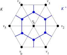
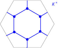
* The faces or cells of <math display="inline">K^*</math> are the areas enclosed by the new polygons determined by the new edges. For instance, the dual of the vertex <math display="inline">[v_6]</math> is the inner blue hexagon in in Figures [[#3.2 Dual mesh|11]](b) and [[#3.2 Dual mesh|11]](c) and will be denoted by <math display="inline">[v_6]^*</math>. | * The faces or cells of <math display="inline">K^*</math> are the areas enclosed by the new polygons determined by the new edges. For instance, the dual of the vertex <math display="inline">[v_6]</math> is the inner blue hexagon in in Figures [[#3.2 Dual mesh|11]](b) and [[#3.2 Dual mesh|11]](c) and will be denoted by <math display="inline">[v_6]^*</math>. | ||
| − | + | {| style="text-align: center; border: 1px solid #BBB; margin: 1em auto; width: auto;max-width: auto;" | |
| − | + | ||
| − | {| | + | |
|- | |- | ||
| − | + | | style="padding:10px;"| [[Image:Review_239195285364_6808_text-boundary04-eps-converted-to.png|220px|]] | |
| − | + | | style="padding:10px;"|[[Image:Review_239195285364_2587_text-Dual00-eps-converted-to.png|220px|]] | |
| − | + | | style="padding:10px;"|[[File:Review_239195285364_6445_Dual01-eps-converted-to.jpg|200px|]] | |
| − | + | |- style="text-align: center; font-size: 75%;" | |
| − | + | | (a) | |
| − | ''</ | + | | (b) |
| + | | (c) | ||
| + | |- style="text-align: center; font-size: 75%;" | ||
| + | | colspan="3" style="padding:10px;"| '''Figure 11'''. Dual mesh construction. (a) Triangular mesh <math>K</math>. (b) Dual mesh <math>K^*</math> superimposed on the mesh <math>K</math>. (c) Dual mesh <math>K^*</math> | ||
|} | |} | ||
| − | |||
| − | |||
| − | |||
The orientation of the dual edges is given by the following recipe. If we have two adjacent triangles oriented as in Figure [[#3.2 Dual mesh|12]](a), the dual edge crossing the edge of adjacency is oriented as in Figure [[#3.2 Dual mesh|12]](b). | The orientation of the dual edges is given by the following recipe. If we have two adjacent triangles oriented as in Figure [[#3.2 Dual mesh|12]](a), the dual edge crossing the edge of adjacency is oriented as in Figure [[#3.2 Dual mesh|12]](b). | ||
| − | + | {| style="text-align: center; border: 1px solid #BBB; margin: 1em auto; width: auto;max-width: auto;" | |
| − | {| | + | |
|- | |- | ||
| − | + | |style="padding:10px;"| [[Image:Review_239195285364_3618_text-TwoTriangles01-eps-converted-to.png|120px|]] | |
| − | + | | style="padding:10px;"| [[Image:Review_239195285364_1851_text-TwoTriangles02-eps-converted-to.png|120px|]] | |
| + | |- style="text-align: center; font-size: 75%;" | ||
| + | | (a) | ||
| + | | (b) | ||
| + | |- style="text-align: center; font-size: 75%;" | ||
| + | | colspan="2" style="padding:10px;"| '''Figure 12'''. (a) Two adjacent oriented triangles. (b) Compatibly oriented dual edge | ||
|} | |} | ||
| − | |||
| − | |||
| − | |||
===3.3 Boundary operator on the dual mesh=== | ===3.3 Boundary operator on the dual mesh=== | ||
| Line 774: | Line 759: | ||
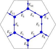
Consider the dual mesh in Figure [[#3.3 Boundary operator on the dual mesh|13]] with the given labels and orientations. | Consider the dual mesh in Figure [[#3.3 Boundary operator on the dual mesh|13]] with the given labels and orientations. | ||
| − | {| | + | {| style="text-align: center; border: 1px solid #BBB; margin: 1em auto; width: auto;max-width: auto;" |
|- | |- | ||
| − | + | | style="padding:10px;"| [[Image:Review_239195285364_5980_text-Dual01a-eps-converted-to.png|220px|]] | |
| − | + | | style="padding:10px;"| [[Image:Review_239195285364_7382_text-Dual01b-eps-converted-to.png|220px|n]] | |
| + | |- style="text-align: center; font-size: 75%;" | ||
| + | | colspan="2" style="padding:10px;"| '''Figure 13'''. Oriented dual mesh | ||
|} | |} | ||
| − | |||
| − | |||
| − | |||
| Line 900: | Line 884: | ||
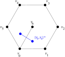
The discretization of the Hodge star <math display="inline">\star </math> uses the geometrical ideas described in Section [[#lb-2.2|2.2]] and the dual mesh. More precisely, the 2D Hodge star operator rotates a vector <math display="inline">90^\circ </math> counterclockwise. For the sake of clarity, let us focus on the edge <math display="inline">[v_0,v_6]</math>, its mesh dual <math display="inline">[v_0,v_6]^*</math> and its Hodge star image <math display="inline">\star [v_0,v_6]</math>. They are represented in Figure [[#3.4 Discrete Hodge star|14]]. | The discretization of the Hodge star <math display="inline">\star </math> uses the geometrical ideas described in Section [[#lb-2.2|2.2]] and the dual mesh. More precisely, the 2D Hodge star operator rotates a vector <math display="inline">90^\circ </math> counterclockwise. For the sake of clarity, let us focus on the edge <math display="inline">[v_0,v_6]</math>, its mesh dual <math display="inline">[v_0,v_6]^*</math> and its Hodge star image <math display="inline">\star [v_0,v_6]</math>. They are represented in Figure [[#3.4 Discrete Hodge star|14]]. | ||
| − | {| | + | {| style="text-align: center; border: 1px solid #BBB; margin: 1em auto; width: auto;max-width: auto;" |
|- | |- | ||
| − | + | | style="padding:10px;"| [[Image:Review_239195285364_9611_text-Dual00a-eps-converted-to.png|220px]] | |
| − | + | | style="padding:10px;"| [[Image:Review_239195285364_4015_text-Dual00aa-eps-converted-to.png|220px]] | |
| + | |- style="text-align: center; font-size: 75%;" | ||
| + | | colspan="2" style="padding:10px;"| '''Figure 14'''. Oriented dual mesh | ||
|} | |} | ||
| − | + | ||
| − | + | ||
Since | Since | ||
| Line 1,053: | Line 1,038: | ||
===4.1 Dual mesh of an arbitrary triangle=== | ===4.1 Dual mesh of an arbitrary triangle=== | ||
| − | In order to explain how to implement DEC for general triangulations, let us consider first a mesh consisting of a single well-centered triangle, as well as its dual mesh ( | + | In order to explain how to implement DEC for general triangulations, let us consider first a mesh consisting of a single well-centered triangle, as well as its dual mesh (Figure [[#4.1 Dual mesh of an arbitrary triangle|15]]). |
| − | {| | + | {| style="text-align: center; border: 1px solid #BBB; margin: 1em auto; width: auto;max-width: auto;" |
|- | |- | ||
| − | + | | style="padding:10px;"| [[Image:Review_239195285364_2549_NewCircumscribedTriangle00.png|260px|]] | |
| − | + | | style="padding:10px;"| [[Image:Review_239195285364_2438_NewCircumscribedTriangle00b.png|280px|]] | |
| + | |- style="text-align: center; font-size: 75%;" | ||
| + | | colspan="2" style="padding:10px;"| '''Figure 15'''. Well-centered triangle and its dual mesh | ||
|} | |} | ||
| − | |||
| − | |||
| − | |||
| Line 1,090: | Line 1,074: | ||
Now consider the cell <math display="inline">[v_3]^* = [v_3,p_3,c,p_2]</math> subdivided as in Figure [[#4.1 Dual mesh of an arbitrary triangle|16]]. | Now consider the cell <math display="inline">[v_3]^* = [v_3,p_3,c,p_2]</math> subdivided as in Figure [[#4.1 Dual mesh of an arbitrary triangle|16]]. | ||
| − | {| | + | {| style="text-align: center; border: 1px solid #BBB; margin: 1em auto; width: auto;max-width: auto;" |
|- | |- | ||
| − | + | | style="padding:10px;"| [[Image:Review_239195285364_1856_NewCircumscribedTriangle00a.png|260px|]] | |
| − | + | |- style="text-align: center; font-size: 75%;" | |
| − | | | + | | colspan="1" style="padding:10px;"| '''Figure 16'''. The subdivision of a 2-dimensional dual cell of a well-centered triangle |
| − | + | |} | |
| − | + | ||
If we deform continuously the triangle <math display="inline">[v_1,v_2,v_3]</math> to become an obtuse triangle as in Figure [[#4.1 Dual mesh of an arbitrary triangle|17]], we see in Figures [[#4.1 Dual mesh of an arbitrary triangle|15]](a) and [[#4.1 Dual mesh of an arbitrary triangle|15]](b) that the area of the blue subtriangle <math display="inline">[v_3,c,p_3]</math> decreases to 0 and in Figure [[#4.1 Dual mesh of an arbitrary triangle|15]](c) that it is completely outside of the triangle and, therefore, must be assigned a negative sign. The same can be said about the 1-dimensional cell <math display="inline">[p_3,c]</math>, which originally is completely contained in the triangle <math display="inline">[v_1,v_2,v_3]</math>, its size reduces to zero as the triangle is deformed (Figures [[#4.1 Dual mesh of an arbitrary triangle|15]](a) and [[#4.1 Dual mesh of an arbitrary triangle|15]](b)), and eventually it is completely outside the triangle <math display="inline">[v_1,v_2,v_3]</math> (Figure [[#4.1 Dual mesh of an arbitrary triangle|15]](c)) and a negative sign must be assigned to it. On the other hand, part of the red subtriangle <math display="inline">[v_3,c,p_2]</math> still intersects the interior of the triangle <math display="inline">[v_1,v_2,v_3]</math> and, therefore, no assignment of sign is needed. Similarly for the segment <math display="inline">[p_2,c]</math>. In terms of numerical simulations, an implementation in terms of determinants contains intrinscally the aforementioned change of signs. | If we deform continuously the triangle <math display="inline">[v_1,v_2,v_3]</math> to become an obtuse triangle as in Figure [[#4.1 Dual mesh of an arbitrary triangle|17]], we see in Figures [[#4.1 Dual mesh of an arbitrary triangle|15]](a) and [[#4.1 Dual mesh of an arbitrary triangle|15]](b) that the area of the blue subtriangle <math display="inline">[v_3,c,p_3]</math> decreases to 0 and in Figure [[#4.1 Dual mesh of an arbitrary triangle|15]](c) that it is completely outside of the triangle and, therefore, must be assigned a negative sign. The same can be said about the 1-dimensional cell <math display="inline">[p_3,c]</math>, which originally is completely contained in the triangle <math display="inline">[v_1,v_2,v_3]</math>, its size reduces to zero as the triangle is deformed (Figures [[#4.1 Dual mesh of an arbitrary triangle|15]](a) and [[#4.1 Dual mesh of an arbitrary triangle|15]](b)), and eventually it is completely outside the triangle <math display="inline">[v_1,v_2,v_3]</math> (Figure [[#4.1 Dual mesh of an arbitrary triangle|15]](c)) and a negative sign must be assigned to it. On the other hand, part of the red subtriangle <math display="inline">[v_3,c,p_2]</math> still intersects the interior of the triangle <math display="inline">[v_1,v_2,v_3]</math> and, therefore, no assignment of sign is needed. Similarly for the segment <math display="inline">[p_2,c]</math>. In terms of numerical simulations, an implementation in terms of determinants contains intrinscally the aforementioned change of signs. | ||
| − | {| | + | {| style="text-align: center; border: 1px solid #BBB; margin: 1em auto; width: auto;max-width: auto;" |
|- | |- | ||
| − | + | | style="text-align: center;padding:10px;"| [[Image:Review_239195285364_9664_NewCircumscribedTriangle01.png|250px|]] | |
| − | + | | style="text-align: center;padding:10px;"| [[Image:Review_239195285364_6104_NewCircumscribedTriangle02.png|250px|]] | |
| + | | style="text-align: center;padding:10px;"| [[Image:Review_239195285364_5608_NewCircumscribedTriangle03.png|250px|]] | ||
| + | |- | ||
| + | | style="text-align: center;font-size: 75%;"|(a) | ||
| + | | style="text-align: center;font-size: 75%;"|(b) | ||
| + | | style="text-align: center;font-size: 75%;"|(c) | ||
| + | |- style="text-align: center; font-size: 75%;" | ||
| + | | colspan="3" style="padding:10px;"| '''Figure 17'''. The subdivision of a 2-dimensional dual cell of a well-centered triangle | ||
|} | |} | ||
| − | + | ||
| − | + | ||
===4.2 Dual mesh of a general triangulation=== | ===4.2 Dual mesh of a general triangulation=== | ||
| Line 1,113: | Line 1,102: | ||
Now consider the well-centered mesh and its dual in Figure [[#4.2 Dual mesh of a general triangulation|18]]. | Now consider the well-centered mesh and its dual in Figure [[#4.2 Dual mesh of a general triangulation|18]]. | ||
| − | + | {| style="text-align: center; border: 1px solid #BBB; margin: 1em auto; width: auto;max-width: auto;" | |
| − | {| | + | |
|- | |- | ||
| − | |[[File:Review_239195285364_3465_NewHexagonalMesh00.png| | + | | style="text-align: center;padding:10px;"| [[File:Review_239195285364_3465_NewHexagonalMesh00.png|260px|]] |
| − | |[[File:Review_239195285364_6131_NewHexagonalMesh01.png| | + | | style="text-align: center;vertical-align: top;padding:10px;"| [[File:Review_239195285364_6131_NewHexagonalMesh01.png|260px|]] |
| + | |- | ||
| + | | style="text-align: center;font-size: 75%;"|(a) | ||
| + | | style="text-align: center;font-size: 75%;"|(b) | ||
|- style="text-align: center; font-size: 75%;" | |- style="text-align: center; font-size: 75%;" | ||
| − | | colspan="2" | '''Figure 18'''. (a) Well-centered triangular mesh of hexagon. (b) Dual mesh | + | | colspan="2" style="padding:10px;"| '''Figure 18'''. (a) Well-centered triangular mesh of hexagon. (b) Dual mesh |
|} | |} | ||
| + | |||
Observe the deformation of the blue-colored dual cell <math display="inline">[v_6]^*</math> in Figure [[#4.2 Dual mesh of a general triangulation|19]](a) as the vertex <math display="inline">v_0</math> is moved to make the triangle <math display="inline">[v_0,v_6,v_5]</math> non-well-centered in Figure [[#4.2 Dual mesh of a general triangulation|19]](b) and the vertex <math display="inline">v_4</math> is moved to make the triangle <math display="inline">[v_4,v_5,v_6]</math> non-well-centered in Figure [[#4.2 Dual mesh of a general triangulation|19]](c). | Observe the deformation of the blue-colored dual cell <math display="inline">[v_6]^*</math> in Figure [[#4.2 Dual mesh of a general triangulation|19]](a) as the vertex <math display="inline">v_0</math> is moved to make the triangle <math display="inline">[v_0,v_6,v_5]</math> non-well-centered in Figure [[#4.2 Dual mesh of a general triangulation|19]](b) and the vertex <math display="inline">v_4</math> is moved to make the triangle <math display="inline">[v_4,v_5,v_6]</math> non-well-centered in Figure [[#4.2 Dual mesh of a general triangulation|19]](c). | ||
| − | {| | + | {| style="text-align: center; border: 1px solid #BBB; margin: 1em auto; width: auto;max-width: auto;" |
|- | |- | ||
| − | + | | style="text-align: center;padding:10px;"| [[File:Review_239195285364_7165_NewHexagonalMesh02.png|250px|]] | |
| − | + | | style="text-align: center;padding:10px;"| [[File:Review_239195285364_6070_NewHexagonalMesh03.png|250px|]] | |
| + | | style="text-align: center;padding:10px;"| [[File:Review_239195285364_6698_NewHexagonalMesh04.png|250px|]] | ||
| + | |- | ||
| + | | style="text-align: center;font-size: 75%;"|(a) | ||
| + | | style="text-align: center;font-size: 75%;"|(b) | ||
| + | | style="text-align: center;font-size: 75%;"|(c) | ||
| + | |- style="text-align: center; font-size: 75%;" | ||
| + | | colspan="3" style="padding:10px;"| '''Figure 19'''. Deformation of a 2-dimensional dual cell as the hexagonal region is deformed | ||
|} | |} | ||
| − | + | ||
| − | + | ||
| − | + | ||
We have colored in red the part of the dual cell <math display="inline">[v_6]^*</math> in Figure [[#4.2 Dual mesh of a general triangulation|16]](c) that must have the opposite orientation of the blue-colored part. Similar considerations apply to the edges. | We have colored in red the part of the dual cell <math display="inline">[v_6]^*</math> in Figure [[#4.2 Dual mesh of a general triangulation|16]](c) that must have the opposite orientation of the blue-colored part. Similar considerations apply to the edges. | ||
| Line 1,162: | Line 1,159: | ||
|} | |} | ||
| − | {| | + | {| style="text-align: center; border: 1px solid #BBB; margin: 1em auto; width: 30%" |
|- | |- | ||
| − | + | |style="padding:10px;"| [[Image:Review_239195285364_5542_Fig_6_circle_prb.png|260px|]] | |
| − | + | |- style="text-align: center; font-size: 75%;" | |
| + | | colspan="1" style="padding:10px;"| '''Figure 20'''. Disk of radius one with difussion constant <math>k=1</math>, subject to a heat source <math>q=-1</math> | ||
|} | |} | ||
| − | |||
| − | |||
The meshes used in this example are shown in Figure [[#5.1 First example|21]] and vary from very coarse to very fine. | The meshes used in this example are shown in Figure [[#5.1 First example|21]] and vary from very coarse to very fine. | ||
| + | {| style="text-align: center; border: 1px solid #BBB; margin: 1em auto; width: auto;max-width: auto;" | ||
| + | |- | ||
| + | | style="text-align: center;padding:10px;"| [[Image:Review_239195285364_2714_Fig_7_circle_msh1.png|150px|]] | ||
| + | | style="text-align: center;padding:10px;"| [[Image:Review_239195285364_3494_Fig_7_circle_msh2.png|150px|]] | ||
| + | | style="text-align: center;padding:10px;"| [[Image:Review_239195285364_1920_Fig_7_circle_msh3.png|150px|]] | ||
| + | |<math> {\quad }</math> | ||
| + | |- | ||
| + | | style="text-align: center;font-size: 75%;"|(a) | ||
| + | | style="text-align: center;font-size: 75%;"|(b) | ||
| + | | style="text-align: center;font-size: 75%;"|(c) | ||
| + | |<math> {\quad }</math> | ||
| + | |- | ||
| + | | colspan="2" style="text-align: center;padding:10px;| [[Image:Review_239195285364_1099_Fig_7_circle_msh4.png|150px|]] | ||
| + | |colspan="2" style="text-align: center;padding:10px;| [[Image:Review_239195285364_9301_Fig_7_circle_msh5.png|150px|]] | ||
| + | |- | ||
| + | | colspan="2" style="text-align: center;font-size: 75%;"|(d) | ||
| + | | colspan="2" style="text-align: center;font-size: 75%;"|(e) | ||
| + | |- | ||
| + | |- style="text-align: center; font-size: 75%;" | ||
| + | | colspan="4" style="padding:10px;"| '''Figure 21'''. Meshes for unit disk | ||
| + | |} | ||
| + | |||
| + | <!-- | ||
{| class="floating_imageSCP" style="text-align: center;" | {| class="floating_imageSCP" style="text-align: center;" | ||
|- | |- | ||
| Line 1,182: | Line 1,201: | ||
|} | |} | ||
<div class="center" style="width: auto; margin-left: auto; margin-right: auto;"> | <div class="center" style="width: auto; margin-left: auto; margin-right: auto;"> | ||
| − | <span style="text-align: center; font-size: 75%;">'''Figure 21'''. Meshes for unit disk</span></div> | + | <span style="text-align: center; font-size: 75%;">'''Figure 21'''. Meshes for unit disk</span></div>--> |
| − | The numerical results for the maximum temperature value (<math display="inline">u(0,0)=10.25</math>) are exemplified in Table [[#5.1 First example|1]] where | + | The numerical results for the maximum temperature value (<math display="inline">u(0,0)=10.25</math>) are exemplified in Table [[#5.1 First example|1]] where a comparison with the Finite Element Method with linear interpolation functions (FEML) is also shown. The FEML methodology that we used in the comparison can be consulted <span id='citeF-13'></span><span id='citeF-12'></span><span id='citeF-2'></span>[[#cite-13|[2,12,13]]]. For the sake of completeness in our comparison, here we compute the flux vectors in the same way as in FEML. |
| + | <div class="center" style="font-size: 75%;">'''Table 1'''. Maximum temperature and Flux magnitude values in the numerical simulation</div> | ||
| − | {| | + | {| style="margin: 1em auto 0.1em auto;border-collapse: collapse;font-size:85%;width:75%;" |
|- | |- | ||
| − | | | + | | style="border-top: 1pt solid black;text-align: left;"|'''Mesh''' |
| − | + | | style="border-top: 1pt solid black;text-align: center;"|'''#nodes''' | |
| + | | style="border-top: 1pt solid black;text-align: center;"| '''#elements''' | ||
| + | | colspan="2" style="border-top: 1pt solid black;text-align: center;"|'''Max. Temp. Value''' | ||
| + | | colspan="2" style="border-top: 1pt solid black;text-align: center;"|'''Max. Flux Magnitude''' | ||
|- | |- | ||
| − | | style="text-align: center;" | | + | | |
| − | | | + | | |
| − | + | | | |
| − | | | + | |style="text-align: center;"|DEC |
| + | | style="text-align: center;"|FEML | ||
| + | |style="text-align: center;"|DEC | ||
| + | | style="text-align: center;"|FEML | ||
| + | |- | ||
| + | | style="border-top: 1pt solid black;text-align: left;"| Figure (a) | ||
| + | | style="border-top: 1pt solid black;text-align: center;"|9 | ||
| + | | style="border-top: 1pt solid black;text-align: center;"|8 | ||
| + | | style="border-top: 1pt solid black;text-align: center;"|10.250 | ||
| + | | style="border-top: 1pt solid black;text-align: center;"|10.285 | ||
| + | | style="border-top: 1pt solid black;text-align: center;"|0.270 | ||
| + | | style="border-top: 1pt solid black;text-align: center;"|0.307 | ||
| + | |- | ||
| + | | style="text-align: left;"| Figure (b) | ||
| + | | style="text-align: center;"|17 | ||
| + | | style="text-align: center;"|20 | ||
| + | | style="text-align: center;"|10.250 | ||
| + | | style="text-align: center;"|10.237 | ||
| + | | style="text-align: center;"|0.388 | ||
| + | | style="text-align: center;"|0.405 | ||
| + | |- | ||
| + | | style="text-align: left;"| Figure (c) | ||
| + | | style="text-align: center;"|41 | ||
| + | | style="text-align: center;"|56 | ||
| + | | style="text-align: center;"|10.250 | ||
| + | | style="text-align: center;"|10.246 | ||
| + | | style="text-align: center;"|0.449 | ||
| + | | style="text-align: center;"|0.453 | ||
| + | |- | ||
| + | | style="text-align: left;"| Figure (d) | ||
| + | | style="text-align: center;"|713 | ||
| + | | style="text-align: center;"|1304 | ||
| + | | style="text-align: center;"|10.250 | ||
| + | | style="text-align: center;"|10.250 | ||
| + | | style="text-align: center;"|0.491 | ||
| + | | style="text-align: center;"|0.492 | ||
| + | |- | ||
| + | | style="text-align: left;border-bottom: 1pt solid black;"| Figure (e) | ||
| + | | style="text-align: center;border-bottom: 1pt solid black;"|42298 | ||
| + | | style="text-align: center;border-bottom: 1pt solid black;"|83346 | ||
| + | | style="text-align: center;border-bottom: 1pt solid black;"|10.250 | ||
| + | | style="text-align: center;border-bottom: 1pt solid black;"|10.250 | ||
| + | | style="text-align: center;border-bottom: 1pt solid black;"|0.496 | ||
| + | | style="text-align: center;border-bottom: 1pt solid black;"|0.496 | ||
|} | |} | ||
| Line 1,202: | Line 1,268: | ||
The temperature distribution and Flux magnitude fields for the finest mesh are shown in Figure [[#5.1 First example|22]]. | The temperature distribution and Flux magnitude fields for the finest mesh are shown in Figure [[#5.1 First example|22]]. | ||
| − | {| | + | {| style="text-align: center; border: 1px solid #BBB; margin: 1em auto; width: auto;max-width: auto;" |
|- | |- | ||
| − | + | | style="text-align: center;padding:10px;vertical-align:center;"| [[Image:Review_239195285364_7846_Fig_8_circle_contour_temp.png|200px|]] | |
| − | + | | style="text-align: center;padding:10px;vertical-align:center;"| [[Image:Review_239195285364_1490_Fig_8_circle_contour_flux.png|200px|]] | |
| + | |- | ||
| + | | style="text-align: center;font-size: 75%;"|(a) | ||
| + | | style="text-align: center;font-size: 75%;"|(b) | ||
| + | |- style="text-align: center; font-size: 75%;" | ||
| + | | colspan="2" style="padding:10px;"| '''Figure 22'''. Temperature distribution and Flux magnitude fields for the finest mesh | ||
|} | |} | ||
| − | |||
| − | |||
Figures [[#5.1 First example|23]](a), [[#5.1 First example|23]](b) and [[#5.1 First example|23]](c) show the graphs of the temperature and flux magnitude values along a diameter of the circle for the different meshes of Figures [[#5.1 First example|23]](b), [[#5.1 First example|23]](c) and [[#5.1 First example|23]](d) respectively. | Figures [[#5.1 First example|23]](a), [[#5.1 First example|23]](b) and [[#5.1 First example|23]](c) show the graphs of the temperature and flux magnitude values along a diameter of the circle for the different meshes of Figures [[#5.1 First example|23]](b), [[#5.1 First example|23]](c) and [[#5.1 First example|23]](d) respectively. | ||
| − | {| | + | {| style="text-align: center; border: 1px solid #BBB; margin: 1em auto; width: auto;max-width: auto;" |
|- | |- | ||
| − | | (a) | + | | style="text-align: center;vertical-align:center;"| (a) |
| − | |[[Image:Review_239195285364_4472_Fig23a_circle.png| | + | |style="text-align: center;padding:10px;"|[[Image:Review_239195285364_4472_Fig23a_circle.png|360px|]] |
| − | |[[Image:Review_239195285364_6864_Fig23a_circle-flux.png| | + | |style="text-align: center;padding:10px;"|[[Image:Review_239195285364_6864_Fig23a_circle-flux.png|360px|]] |
|- | |- | ||
| − | | (b) | + | | style="text-align: center;vertical-align:center;"| (b) |
| − | |[[Image:Review_239195285364_4411_Fig23b_circle.png| | + | |style="text-align: center;padding:10px;"|[[Image:Review_239195285364_4411_Fig23b_circle.png|360px|]] |
| − | |[[Image:Review_239195285364_6460_Fig23b_circle-flux.png| | + | |style="text-align: center;padding:10px;"|[[Image:Review_239195285364_6460_Fig23b_circle-flux.png|360px|]] |
|- | |- | ||
| − | | (c) | + | | style="text-align: center;vertical-align:center;"| (c) |
| − | |[[Image:Review_239195285364_8672_Fig23c_circle.png| | + | |style="text-align: center;padding:10px;"|[[Image:Review_239195285364_8672_Fig23c_circle.png|360px|]] |
| − | |[[Image:Review_239195285364_5450_Fig23c_circle-flux.png| | + | |style="text-align: center;padding:10px;"|[[Image:Review_239195285364_5450_Fig23c_circle-flux.png|360px|]] |
|- style="text-align: center; font-size: 75%;" | |- style="text-align: center; font-size: 75%;" | ||
| colspan="3" style="padding-top:10px;"| '''Figure 23'''. Temperature and Flux magnitude graphs along a diameter of the circle for different meshes: (a) Graphs for the Mesh in Figure [[#5.1 First example|23]](b); (b) Graphs for the Mesh in Figure [[#5.1 First example|23]](c); (c) Graphs for the Mesh in Figure [[#5.1 First example|23]](d) | | colspan="3" style="padding-top:10px;"| '''Figure 23'''. Temperature and Flux magnitude graphs along a diameter of the circle for different meshes: (a) Graphs for the Mesh in Figure [[#5.1 First example|23]](b); (b) Graphs for the Mesh in Figure [[#5.1 First example|23]](c); (c) Graphs for the Mesh in Figure [[#5.1 First example|23]](d) | ||
| Line 1,231: | Line 1,300: | ||
| − | As can be seen from Table [[#5.1 First example|1]] and Figure [[#5.1 First example| | + | As can be seen from Table [[#5.1 First example|1]] and Figure [[#5.1 First example|20]], DEC behaves very well on coarse meshes. Note that the maximum temperature values calculated with DEC matches the exact theoretical value even on coarse meshes. As expected, the results of DEC and FEML are similar for fine meshes. We would also like to point out the the computational costs of DEC and FEML are very similar. |
===5.2 Second example=== | ===5.2 Second example=== | ||
| − | In this example, we consider a region in the plane whose boundary consists of segments of a straight line, a circle, a parabola, a cubic and an ellipse ( | + | In this example, we consider a region in the plane whose boundary consists of segments of a straight line, a circle, a parabola, a cubic and an ellipse (Figure [[#5.2 Second example|24]]). |
| − | + | {| style="text-align: center; border: 1px solid #BBB; margin: 1em auto; width: auto;max-width: auto;" | |
| − | {| | + | |
|- | |- | ||
| − | |[[Image:Review_239195285364_6878_Fig_10a_patata_prb.png| | + | | style="text-align: center;padding:10px;"| [[Image:Review_239195285364_6878_Fig_10a_patata_prb.png|360px|]] |
| − | |[[Image:Review_239195285364_1159_Fig_10b_patata_geom.png| | + | | style="text-align: center;vertical-align: top;padding:10px;"| [[Image:Review_239195285364_1159_Fig_10b_patata_geom.png|360px|]] |
|- style="text-align: center; font-size: 75%;" | |- style="text-align: center; font-size: 75%;" | ||
| − | | colspan="2" | '''Figure 24'''. Region with linear, quadratic and cubic boundary segments, together with boundary conditions | + | | colspan="2" style="padding:10px;"| '''Figure 24'''. Region with linear, quadratic and cubic boundary segments, together with boundary conditions |
|} | |} | ||
| Line 1,249: | Line 1,317: | ||
The meshes used in this example are shown in Figure [[#5.2 Second example|25]] and vary from coarse to very fine. | The meshes used in this example are shown in Figure [[#5.2 Second example|25]] and vary from coarse to very fine. | ||
| − | {| | + | {| style="text-align: center; border: 1px solid #BBB; margin: 1em auto; width: auto;max-width: auto;" |
|- | |- | ||
| − | |[[Image:Review_239195285364_6629_Fig_11c_patata_m2.png|260px|]] | + | | style="text-align: center;padding:10px;"| [[Image:Review_239195285364_6629_Fig_11c_patata_m2.png|260px|]] |
| − | |[[Image:Review_239195285364_5402_Fig_11d_patata_m3.png|260px|]] | + | | style="text-align: center;padding:10px;"| [[Image:Review_239195285364_5402_Fig_11d_patata_m3.png|260px|]] |
| − | |[[Image:Review_239195285364_3774_Fig_11e_patata_m4.png|260px|]] | + | | style="text-align: center;padding:10px;"| [[Image:Review_239195285364_3774_Fig_11e_patata_m4.png|260px|]] |
|- | |- | ||
| − | | (a) | + | | style="text-align: center;font-size: 75%;"|(a) |
| − | | (b) | + | | style="text-align: center;font-size: 75%;"|(b) |
| − | | (c) | + | | style="text-align: center;font-size: 75%;"|(c) |
|- style="text-align: center; font-size: 75%;" | |- style="text-align: center; font-size: 75%;" | ||
| − | | colspan="3" | '''Figure 25'''. Three of the meshes used in the first example | + | | colspan="3" style="padding:10px;"| '''Figure 25'''. Three of the meshes used in the first example |
|} | |} | ||
| − | + | ||
We set | We set | ||
| Line 1,272: | Line 1,340: | ||
The numerical results for the maximum temperature and flux magnitude values are exemplified in Table [[#5.2 Second example|2]]. | The numerical results for the maximum temperature and flux magnitude values are exemplified in Table [[#5.2 Second example|2]]. | ||
| − | + | <div class="center" style="font-size: 75%;">'''Table 2'''. Numerical simulation results</div> | |
| + | |||
| + | {| style="margin: 1em auto 0.1em auto;border-collapse: collapse;font-size:85%;width:75%;" | ||
|- | |- | ||
| − | | | + | | style="border-top: 1pt solid black;text-align: left;"|'''Mesh''' |
| − | + | | style="border-top: 1pt solid black;text-align: center;"|'''#nodes''' | |
| + | | style="border-top: 1pt solid black;text-align: center;"| '''#elements''' | ||
| + | | colspan="2" style="border-top: 1pt solid black;text-align: center;"|'''Max. Temp. Value''' | ||
| + | | colspan="2" style="border-top: 1pt solid black;text-align: center;"|'''Max. Flux Magnitude''' | ||
| + | |- | ||
| + | | | ||
| + | | | ||
| + | | | ||
| + | |style="text-align: center;"|DEC | ||
| + | | style="text-align: center;"|FEML | ||
| + | |style="text-align: center;"|DEC | ||
| + | | style="text-align: center;"|FEML | ||
| + | |- | ||
| + | | style="border-top: 1pt solid black;text-align: left;"| Figure 21(a) | ||
| + | | style="border-top: 1pt solid black;text-align: center;"|162 | ||
| + | | style="border-top: 1pt solid black;text-align: center;"|268 | ||
| + | | style="border-top: 1pt solid black;text-align: center;"|129.07 | ||
| + | | style="border-top: 1pt solid black;text-align: center;"|128.92 | ||
| + | | style="border-top: 1pt solid black;text-align: center;"|467.22 | ||
| + | | style="border-top: 1pt solid black;text-align: center;"|467.25 | ||
| + | |- | ||
| + | | style="text-align: left;"| Figure 21(b) | ||
| + | | style="text-align: center;"|678 | ||
| + | | style="text-align: center;"|1223 | ||
| + | | style="text-align: center;"|129.71 | ||
| + | | style="text-align: center;"|129.70 | ||
| + | | style="text-align: center;"|547.87 | ||
| + | | style="text-align: center;"|548.42 | ||
| + | |- | ||
| + | | style="text-align: left;"| Figure 21(c) | ||
| + | | style="text-align: center;"|9489 | ||
| + | | style="text-align: center;"|18284 | ||
| + | | style="text-align: center;"|130.00 | ||
| + | | style="text-align: center;"|130.00 | ||
| + | | style="text-align: center;"|591.58 | ||
| + | | style="text-align: center;"|591.63 | ||
| + | |- | ||
| + | | style="text-align: left;"| | ||
| + | | style="text-align: center;"|27453 | ||
| + | | style="text-align: center;"|53532 | ||
| + | | style="text-align: center;"|130.01 | ||
| + | | style="text-align: center;"|130.01 | ||
| + | | style="text-align: center;"|597.37 | ||
| + | | style="text-align: center;"|597.38 | ||
|- | |- | ||
| − | | style="text-align: | + | | style="text-align: left;border-bottom: 1pt solid black;"| |
| − | + | | style="text-align: center;border-bottom: 1pt solid black;"|651406 | |
| − | + | | style="text-align: center;border-bottom: 1pt solid black;"|1295960 | |
| − | + | | style="text-align: center;border-bottom: 1pt solid black;"|130.02 | |
| − | + | | style="text-align: center;border-bottom: 1pt solid black;"|130.02 | |
| − | + | | style="text-align: center;border-bottom: 1pt solid black;"|602.19 | |
| − | | | + | | style="text-align: center;border-bottom: 1pt solid black;"|602.19 |
| − | + | ||
| − | | | + | |
|} | |} | ||
| Line 1,291: | Line 1,402: | ||
The temperature and flux-magnitude distribution fields are shown in Figure [[#5.2 Second example|26]]. | The temperature and flux-magnitude distribution fields are shown in Figure [[#5.2 Second example|26]]. | ||
| − | {| | + | {| style="text-align: center; border: 1px solid #BBB; margin: 1em auto; width: auto;max-width: auto;" |
|- | |- | ||
| − | |[[Image:Review_239195285364_1649_Fig_14_patata2_contour_temp.png|260px]] | + | | style="text-align: center;padding:10px;"| [[Image:Review_239195285364_1649_Fig_14_patata2_contour_temp.png|260px]] |
| − | |[[Image:Review_239195285364_8633_Fig_14_patata2_contour_flux.png|260px]] | + | | style="text-align: center;vertical-align: top;padding:10px;"| [[Image:Review_239195285364_8633_Fig_14_patata2_contour_flux.png|260px]] |
|- | |- | ||
| − | | (a) | + | | style="text-align: center;font-size: 75%;"|(a) |
| − | | (b) | + | | style="text-align: center;font-size: 75%;"|(b) |
|- style="text-align: center; font-size: 75%;" | |- style="text-align: center; font-size: 75%;" | ||
| − | | colspan=" | + | | colspan="2" style="padding:10px;"| '''Figure 26'''. Temperature and Flux magnitude distribution fields |
|} | |} | ||
| Line 1,305: | Line 1,416: | ||
Figure [[#5.2 Second example|27]] shows the graphs of the temperature and the flux magnitude along a horizontal line crossing the elliptical boundary for the first two meshes. | Figure [[#5.2 Second example|27]] shows the graphs of the temperature and the flux magnitude along a horizontal line crossing the elliptical boundary for the first two meshes. | ||
| − | {| | + | {| style="text-align: center; border: 1px solid #BBB; margin: 1em auto; width: auto;max-width: auto;" |
|- | |- | ||
| − | | (a) | + | | style="text-align: center;vertical-align:center;padding:10px;"| (a) |
| − | |[[Image:Review_239195285364_4170_Fig_15b_patata2_m2.png| | + | |style="text-align: center;padding:10px;"|[[Image:Review_239195285364_4170_Fig_15b_patata2_m2.png|360px]] |
| − | |[[Image:Review_239195285364_1673_Fig_15b_patata2_m2_flux.png| | + | |style="text-align: center;padding:10px;"|[[Image:Review_239195285364_1673_Fig_15b_patata2_m2_flux.png|360px]] |
|- | |- | ||
| − | | (b) | + | | style="text-align: center;vertical-align:center;padding:10px;"| (b) |
| − | |[[Image:Review_239195285364_8948_Fig_15c_patata2_m3.png| | + | |style="text-align: center;padding:10px;"|[[Image:Review_239195285364_8948_Fig_15c_patata2_m3.png|360px]] |
| − | |[[Image:Review_239195285364_8624_Fig_15c_patata2_m3_flux.png| | + | |style="text-align: center;padding:10px;"|[[Image:Review_239195285364_8624_Fig_15c_patata2_m3_flux.png|360px]] |
|- style="text-align: center; font-size: 75%;" | |- style="text-align: center; font-size: 75%;" | ||
| − | | colspan="3" style="padding | + | | colspan="3" style="padding:10px;"| '''Figure 27''' Temperature and Flux magnitude graphs along a horizontal line crossing the elliptical boundary for the first two meshes |
|} | |} | ||
| Line 1,337: | Line 1,448: | ||
The second named author was partially supported by a grant of CONACYT, and would like to thank the International Centre for Numerical Methods in Engineering (CIMNE) and the University of Swansea for their hospitality. We gratefully acknowledge the support of NVIDIA Corporation with the donation of the Titan X Pascal GPU used for this research. | The second named author was partially supported by a grant of CONACYT, and would like to thank the International Centre for Numerical Methods in Engineering (CIMNE) and the University of Swansea for their hospitality. We gratefully acknowledge the support of NVIDIA Corporation with the donation of the Titan X Pascal GPU used for this research. | ||
| − | == | + | ==References== |
<div class="auto" style="width: auto; margin-left: auto; margin-right: auto;font-size: 85%;"> | <div class="auto" style="width: auto; margin-left: auto; margin-right: auto;font-size: 85%;"> | ||
<div id="cite-1"></div> | <div id="cite-1"></div> | ||
| − | [[#citeF-1|[1]]] D. | + | [[#citeF-1|[1]]] Arnold D., Falk R., WintherR. Finite element exterior calculus: From Hodge theory to numerical stability. Bulletin of the American Mathematical Society, 47(2):281-354, 2010. |
<div id="cite-2"></div> | <div id="cite-2"></div> | ||
| − | [[#citeF-2|[2]]] | + | [[#citeF-2|[2]]] Botello S., Moreles M.A., Oñate E. Módulo de aplicaciones del método de los elementos finitos para resolver la ecuación de Poisson: MEFIPOISS. Aula CIMNE-CIMAT, Septiembre 2010, ISBN 978-84-96736-95-5. |
<div id="cite-3"></div> | <div id="cite-3"></div> | ||
| − | [[#citeF-3|[3]]] E. | + | [[#citeF-3|[3]]] Cartann E. Sur certaines expressions différentielles et le problème de Pfaff. Annales Scientifiques de l'École Normale Supérieure, Série 3, Paris, Gauthier-Villars, 16:239-332, 1899. |
<div id="cite-4"></div> | <div id="cite-4"></div> | ||
| − | [[#citeF-4|[4]]] | + | [[#citeF-4|[4]]] Crane K., de Goes F., Desbrun M., Schröder P. Digital geometry processing with discrete exterior calculus. ACM SIGGRAPH 2013 Courses, ACM, 2013. |
<div id="cite-5"></div> | <div id="cite-5"></div> | ||
| − | [[#citeF-5|[5]]] | + | [[#citeF-5|[5]]] Dassios I., Jivkov A.P., Abu-Muharib A., James P. A mathematical model for plasticity and damage: A discrete calculus formulation. Journal of Computational and Applied Mathematics, 312:27-38, 2017. |
<div id="cite-6"></div> | <div id="cite-6"></div> | ||
| − | [[#citeF-6|[6]]] M. | + | [[#citeF-6|[6]]] Desbrun M., Kanso E., Tong Y. Discrete differential forms for computational modeling. In SIGGRAPH 06: ACM SIGGRAPH 2006 Courses, pp. 39–54, New York, 2006. |
<div id="cite-7"></div> | <div id="cite-7"></div> | ||
| − | [[#citeF-7|[7]]] | + | [[#citeF-7|[7]]] Griebel M., Rieger C., Schier A. Upwind schemes for scalar advection-dominated problems in the discrete exterior calculus. Transport Processes at Fluidic Interfaces, Birkhäuser, Cham, pp. 145-175, 2017. |
<div id="cite-8"></div> | <div id="cite-8"></div> | ||
| − | [[#citeF-8|[8]]] | + | [[#citeF-8|[8]]] Hirani A.N. Discrete exterior calculus. Diss. California Institute of Technology, 2003. |
<div id="cite-9"></div> | <div id="cite-9"></div> | ||
| − | [[#citeF-9|[9]]] | + | [[#citeF-9|[9]]] Hirani A.N., Nakshatrala K.B., Chaudhry J.H. Numerical method for Darcy flow derived using Discrete Exterior Calculus. International Journal for Computational Methods in Engineering Science and Mechanics, 16(3):151-169, 2015. |
<div id="cite-10"></div> | <div id="cite-10"></div> | ||
| − | [[#citeF-10|[10]]] | + | [[#citeF-10|[10]]] Hirani A.N., Kalyanaraman K., VanderZee E.B. Delaunay Hodge star. Comput. Aided Des., 45:540-544, 2013. |
<div id="cite-11"></div> | <div id="cite-11"></div> | ||
| − | [[#citeF-11|[11]]] | + | [[#citeF-11|[11]]] Mohamed M.S., Hirani A.N., Samtaney R. Discrete exterior calculus discretization of incompressible Navier-Stokes equations over surface simplicial meshes. Journal of Computational Physics, 312:175-191, 2016. |
<div id="cite-12"></div> | <div id="cite-12"></div> | ||
| − | [[#citeF-12|[12]]] E. | + | [[#citeF-12|[12]]] Oñate E. 2D Solids. Linear Triangular and Rectangular Elements (chapter 4). In Structural Analysis with the Finite Element Method. Linear Statics, Volume 1: Basis and Solids, CIMNE-Springer, pp. 117-157, Barcelona, 2009, ISBN 978-1-4020-8733-2. |
<div id="cite-13"></div> | <div id="cite-13"></div> | ||
| − | [[#citeF-13|[13]]] | + | [[#citeF-13|[13]]] Zienkiewicz O.C., Taylor R.L., Zhu J.Z. Generalization of the finite element concepts. Galerkin-weighted residual and variational approaches (chapter 3). In The Finite Element Method Set (Sixth Edition), Butterworth-Heinemann, pp. 54-102, Oxford 2005, ISBN 9780750664318. |
</div> | </div> | ||
Latest revision as of 13:17, 28 April 2020
Abstract
We revisit the theory of Discrete Exterior Calculus (DEC) in 2D for general triangulations, relying only on Vector Calculus and Matrix Algebra. We present DEC numerical solutions of the Poisson equation and compare them against those found using the Finite Element Method with linear elements (FEML).
Keywords: Discrete element method, Poisson equation
1. Introduction
The purpose of this paper is to introduce the theory of Discrete Exterior Calculus (DEC) to the widest possible audience and, therefore, we will rely mainly on Vector Calculus and Matrix Algebra. Discrete Exterior Calculus is a relatively new method for solving partial differential equations [8] based on the idea of discretizing the mathematical theory of Exterior Differential Calculus, a theory that goes back to Cartan [3] and is fundamental in the areas of Differential Geometry and Differential Topology. Although Exterior Differential Calculus is an abstract mathematical theory, it has been introduced in various fields such as in digital geometry processing [4], numerical schemes for partial differential equations [1,8], etc.
In his PhD thesis [8], Hirani laid down the fundamental concepts of Discrete Exterior Calculus (DEC), using discrete combinatorial and geometric operations on simplicial complexes (in any dimension), proposing discrete equivalents for differential forms, vector fields, differential and geometric operators, etc. Perhaps the first numerical application of DEC to PDE was given in [9] in order to solve Darcy flow and Poisson's equation. In [7], the authors develop a modification of DEC and show that in simple cases (e.g. flat geometry and regular meshes), the equations resulting from DEC are equivalent to classical numerical schemes such as finite difference or finite volume discretizations. In [11], the authors used DEC to solve the Navier-Stokes equations and, in [5] DEC was used with a discrete lattice model to simulate elasticity, plasticity and failure of isotropic materials.
In this expository paper, we review the various operators of Exterior Differential Calculus in 2D in terms of ordinary vector calculus, and introduce only the geometrical ideas that are essential to the formulation. Among those ideas is that of duality between the differentiation operator (on vector fields) and the boundary operator (on the domain) contained in Green's theorem. This duality is one of the key ideas of the method, which justifies taking the discretized derivative matrix as the transpose of the boundary operator matrix on the given mesh. Another important ingredient is the Hodge star operator, which is hidden in the notation of Vector Calculus. In order to show the necessity of the Hodge star operator, we carry out some simple calculations. In particular, we will introduce the notion of wedge product of vectors which, roughly speaking, helps us assign algebraic objects to parallelograms and carry out algebraic manipulations with them. We present DEC in the simplest terms possible using easy examples. We also review the formulation of DEC for arbitrary meshes, which was first considered in [10]. Performance of the method is tested on the Poisson equation and compared with the Finite Element Method with linear elements (FEML).
The paper is organized as follows. In Section 2, we introduce the wedge product of vectors and the geometric Hodge star operator, and rewrite Green's theorem appropriately in order to display the duality between the differentiation and the boundary operators. In Section 3, we present the operators of DEC (mesh, dual mesh, discrete derivation, discrete Hodge star operator), showing simple examples throughout. In Section 4, we present the formulation of DEC on arbitrary triangulations. In Section 5, we present the numerical solution of a Poisson equation with DEC and FEML, in order to compare their performance. In Section 6, we present our conclusions.
2. 2D Exterior Differential Calculus as Vector Calculus
In this section we introduce two geometric operators (the wedge product and the Hodge star) and explain how to use them together with the gradient operator in order to obtain the Laplacian.
2.1 Wedge product for vectors in R²
Let be vectors in . We can assign to these vector the parallelogram they span, and to such a parallelogram its area. The latter is equal to the determinant of the transformation matrix sending to respectively. In Exterior Calculus, such a parallelogram is regarded as an algebraic object , a bivector, and the set of bivectors is equipped with a vector space structure to form the one-dimensional vector space
|
|
Thus, we have the following spaces
|
|
of scalars, vectors and bivectors, respectively. For instance, the square formed by and is represented by the symbol
|
|
which is read as " wedge " (Figure 1).

|
| Figure 1. Wedge product of two vectors |
In , this represents an “element” of unit area.
Note that if we list the vectors in the opposite order, we have a different orientation and, therefore, the algebraic objects must satisfy (Figure 2).

|
| Figure 2. Change of orientation of the parallelogram implies anticommutativity in the wedge product of two vectors |
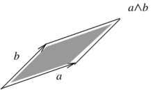
More generally, given two vectors , their wedge product looks as follows (Figure 3).
|
| Figure 3. The wedge product of the vectors and |
The properties of the wedge product are
- it is anticommutative: (Figure 4)

|

|
| Figure 4. Anticommutativity of the wedge product | |
- since it is a parallelogram with area zero (Figure 5)

|
| Figure 5. Parallelogram with very small area, depicting what happens when tends to |
- it is distributive
|
|
- it is associative
|
|
For example, let
|
|
Then
|
|
i.e. the determinant
|
|
times the canonical bivector/square .
2.2 Hodge star operator for vectors in R²
Now consider the following situation: given the vector , find another vector such that the parallelogram that they form has area . It is readily seen that, for instance, are all solutions. Requiring orthogonality and standard orientation, we see that is the unique solution. This process is summarized in the Hodge star operator, which basically says that the complementary vector for is , and the one for is ,
|
|
In general, the equation that defines the Hodge star operator for any given vector is the following
|
|
for every . In particular, if we take ,
|
|
which means that and form a square of area . Thus, the Hodge star operator on a vector can be thought of as finding the vector that makes with a positively oriented square of area .
It is somewhat less intuitive to work out the Hodge star of a bivector. First of all, we have to treat bivectors as vectors of a different space, namely the space of bivectors . Secondly, the length of a bivector is its area
|
|
Thus, the defining equation of the Hodge star applied to and reads as follows
|
|
which means
|
|
Since is already a bivector, must be a scalar, i.e.
|
|
When and we have
|
|
Finally, the Hodge star of a number is a bivector, i.e.
|
|
2.3 The Laplacian
Let and consider the gradient
|
|
Apply the Hodge star operator to it
|
|
Now take the gradient of each coefficient function together with wedge product
|
|
By taking the Hodge star of this last expression we get the ordinary Laplacian of
|
|
Remarks.
(i) This rather convoluted looking way of computing the Laplacian of a function is based on Exterior Differential Calculus, a theory that generalizes the operators of vector calculus (gradient, curl and divergence) to arbitrary dimensions, and is the basis for the differential topological theory of deRham cohomology.
(ii) We would like to emphasize the necessity of using the Hodge star operator in order to make the combination of differentiation and wedge product produce the correct answer.
2.4 Duality in Green's theorem
Green's theorem states that for a vector field defined on a region ,
|
|
In this section, we will explain how this identity encodes a duality between the operator of differentiation and that of taking the boundary of the domain of integration.
2.4.1 Rewriting Green's theorem
Note that if is a vector field, we can write it as
|
|
Then, we can apply the gradient operator together with wedge product in the following fashion
|
|
Note that we have defined a new operator which combines differentiation and wedge product. Applying the Hodge star operator we obtain
|
|
i.e. the integrand of the left hand side of the identity of integrals in Green's theorem. Thus, as a first step, Green's theorem can be rewritten as follows:
|
|
2.4.2 The duality in Green's theorem
Let us recall the following fact from Linear Algebra. Given a linear transformation of Euclidean space , the transpose satisfies
|
|
for any two vectors , where denotes the standard inner/dot product. In fact, such an identity characterizes the transpose .
Now, let us do the following notational trick: substitute the integration symbols in Green's theorem by as follows:
|
|
where is the boundary of the region. Using this notational change, Green's theorem reads as follows
|
|
Roughly speaking, this means that the differential operator is the transpose of the boundary operator by means of the product .
Remark. The previous observation is fundamental in the development of DEC, since the boundary operator is well understood and easy to calculate on meshes.
3. Discrete Exterior Calculus
Now we will discretize the differentiation operator presented above. We will start by describing the discrete version of the boundary operator on simplices/triangles. Afterwards, we will treat the differentiation operator as the transpose of the boundary operator.
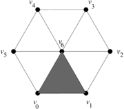
We are interested in using certain geometric subsets of a given triangular mesh of a 2D region. Such subsets include vertices/nodes, edges/sides and faces/triangles. We will describe each one of them by means of the ordered list of vertices whose convex closure constitutes the subset of interest. For instance, consider the triangular mesh of the planar hexagonal region in Figure 6,
|
| Figure 6. Triangular mesh of a planar hexagonal region |
where the shaded triangle will be denoted by , and its edge joining the vertices and will be denoted by . For the sake of notational consistency, we will denote the vertices also enclosed in brackets, e.g. .
3.1 Boundary operator and discrete derivative
There is a well known boundary operator for oriented triangles, edges and points:
- For points/vertices:

|
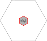
| Figure 7. Boundary of a vertex: |
- For sides/edges:

|
| Figure 8. Boundary of an edge: |
- For faces/triangles:

|
| Figure 9. Boundary of a face: |
Example. Let us consider again the mesh of the planar hexagonal (with oriented triangles) in Figure 10.

|
| Figure 10. Oriented triangular mesh of a planar hexagonal region |
We will denote a triangle by the list of its vertices listed in order according to the orientation of the tringle. Thus, we have the following ordered lists:
- list of faces
|
|
- list of edges
|
|
- list of vertices
|
|
A key idea in DEC is to consider each face as an element of a basis of a vector space. Namely, column coordinate vectors are associated to faces as follows:
|
|
Similarly, coordinate vectors are associated to the edges
|
|
Finally, we do the same with the vertices
|
|
Now, if we take the boundary of each face, we have
|
|
which, under the previous assignments of coordinate vectors, corresponds to the linear transformation given by the following matrix which will multiply the column coordinate vectors on the left
|
|
where the subindices in indicate that we are taking the boundary of 2-dimensional elements and obtaining 1-dimensional ones. Similarly, taking the boundaries of all the edges gives
|
|
which, under the previous assignments of coordinate vectors, corresponds to the linear transformation given by the following matrix
|
|
Remark. Note how these matrices encode different levels of connectivity with orientations, such as who are the edges of which oriented triangle, or which are the end points of a given oriented edge.
Due to the duality between and , we can define the discretiztion of by
|
|
For instance, we see that the operator reads as follows
|
|
3.2 Dual mesh
In order to discretize the Hodge star operator, we must first introduce the notion of the dual mesh of a triangular mesh.
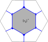
Consider the triangular mesh in Figure 11(a). The construction of the dual mesh is carried out as follows:
- The vertices of the dual mesh are the circumcenters of the faces/triangles of the original mesh (the blue dots in Figures 11(b) and 11(c)). For instance, the dual of the face will be denoted by .
- The edges of are the straight line segments joining the circumcenters of two adjacent triangles (those which share an edge). Note that the resulting line segments are orthogonal to one of the original edges (the blue straight line segments in in Figures 11(b) and 11(c)). For instance, the dual of the edge will be denoted by .
- The faces or cells of are the areas enclosed by the new polygons determined by the new edges. For instance, the dual of the vertex is the inner blue hexagon in in Figures 11(b) and 11(c) and will be denoted by .

|
|
|
| (a) | (b) | (c) |
| Figure 11. Dual mesh construction. (a) Triangular mesh . (b) Dual mesh superimposed on the mesh . (c) Dual mesh | ||
The orientation of the dual edges is given by the following recipe. If we have two adjacent triangles oriented as in Figure 12(a), the dual edge crossing the edge of adjacency is oriented as in Figure 12(b).

|

|
| (a) | (b) |
| Figure 12. (a) Two adjacent oriented triangles. (b) Compatibly oriented dual edge | |
3.3 Boundary operator on the dual mesh
Consider the dual mesh in Figure 13 with the given labels and orientations.

|
|
| Figure 13. Oriented dual mesh | |
The boundary operator is applied in a similar fashion as it was applied to triangles. In this case we have
|
|
If we assign coordinate vectors to the dual faces and the dual edges as before
|
|
and
|
|
we have the associated matrix
|
|
Notice that
|
|
which arises from the duality between the two meshes [6]. In general, the discrete differential to be applied is
|
|
3.4 Discrete Hodge star
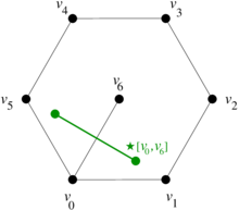
The discretization of the Hodge star uses the geometrical ideas described in Section 2.2 and the dual mesh. More precisely, the 2D Hodge star operator rotates a vector counterclockwise. For the sake of clarity, let us focus on the edge , its mesh dual and its Hodge star image . They are represented in Figure 14.
|
|
| Figure 14. Oriented dual mesh | |
Since
|
|
we see that the relationship between the dual edge and the geometric is the following
|
|
As can be seen, when applying the geometric Hodge star to the edges of the mesh, we do not end up in the dual mesh but in multiples of the elements of the dual mesh. Thus, must be scaled to match . If we do this to all the Hodge star images, we get the discrete Hodge star matrix
|
|
where the subindices in indicate that we are sending 1-dimensional elements of the original mesh to 1-dimensional elements of the dual mesh.
Somewhat less intuitive is the meaning of the geometric Hodge star operator on nodes of the original mesh. As we saw in Subsection 2.2,
|
|
which geometrically means that the Hodge star must be a polygon with area equal to 1 (classically, it is a parallelogram, but can also be a hexahedron of area 1 as in this example).
However, in the dual mesh we have the polygon
so that we need to resize as follows
|
|
If we do that for all the vertices, we obtain the discrete Hodge star matrix
|
|
The inverse matrix will deal with the case when we take the Hodge star of the 2D polygons in the dual mesh to obtain points (with weight 1) in the original mesh.
In summary, the various matrices representing the discrete Hodge star operator send elements of the original mesh to elements of the dual mesh.
3.5 DEC applied to 2D Poisson's equation
Consider the 2D Poisson's equation
|
|
As we have seen, this can be rewritten as
|
|
Suppose that we wish to solve the equation using the mesh . Let us denote by and the column vector discretizations of the functions and at the nodes. According to DEC, the first derivation is achieved left-multiplying by the matrix of Subsection 3.1. The resulting column vector is a collection of (unknown) directional derivative values of assigned to the ordered set of edges. At this point we need to transfer such a set of values to the ordered set of dual edges of the dual mesh with the appropriate geometrical scaling, which is achieved multiplying on the left by the matrix of Subsection 3.4. Now, the discrete version of the second derivation is given by left multiplication with the matrix of Subsection 3.3, which gives a column vector of (unknown) values assigned to the ordered set of 2-dimensional cells of the dual mesh. Finally, the task of mapping such values (with the appropriate scaling) to the ordered set of vertices of the original mesh is achieved by left multiplication with the matrix of Subsection 3.4. Thus, the Poisson equation is discretized as the matrix equation
|
|
Later on, it will be convenient to work with the equivalent system
|
|
Note that the DEC-discretization of is not a (discretized) flow vector. It is a collection of values of directional derivatives of , one such value for each oriented edge.
4. DEC for general triangulations
Since the boundary operator is really concerned with the connectivity of the mesh and does not change under deformation of the mesh, the change in the setup of DEC for a deformed mesh must be contained in the discrete Hodge star matrices. Since such matrices are computed in terms of lengths and areas of oriented elements of the mesh, we will now examine how those ingredients transform under deformation, a problem that was first considered in [10].
4.1 Dual mesh of an arbitrary triangle
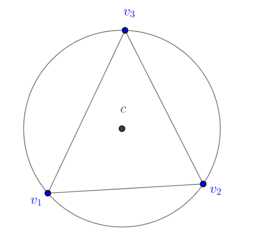
In order to explain how to implement DEC for general triangulations, let us consider first a mesh consisting of a single well-centered triangle, as well as its dual mesh (Figure 15).
|

|
| Figure 15. Well-centered triangle and its dual mesh | |
The dual cells are given as follows:
|
|
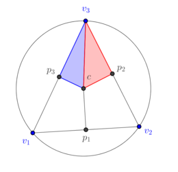
Now consider the cell subdivided as in Figure 16.
|
| Figure 16. The subdivision of a 2-dimensional dual cell of a well-centered triangle |
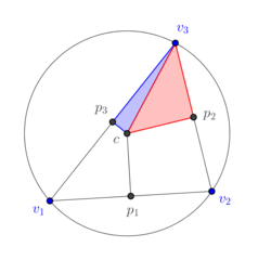
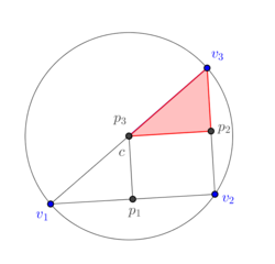
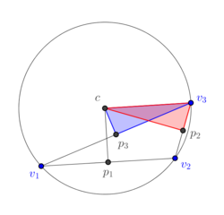
If we deform continuously the triangle to become an obtuse triangle as in Figure 17, we see in Figures 15(a) and 15(b) that the area of the blue subtriangle decreases to 0 and in Figure 15(c) that it is completely outside of the triangle and, therefore, must be assigned a negative sign. The same can be said about the 1-dimensional cell , which originally is completely contained in the triangle , its size reduces to zero as the triangle is deformed (Figures 15(a) and 15(b)), and eventually it is completely outside the triangle (Figure 15(c)) and a negative sign must be assigned to it. On the other hand, part of the red subtriangle still intersects the interior of the triangle and, therefore, no assignment of sign is needed. Similarly for the segment . In terms of numerical simulations, an implementation in terms of determinants contains intrinscally the aforementioned change of signs.
|
|
|
| (a) | (b) | (c) |
| Figure 17. The subdivision of a 2-dimensional dual cell of a well-centered triangle | ||
4.2 Dual mesh of a general triangulation
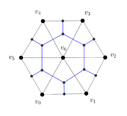
Now consider the well-centered mesh and its dual in Figure 18.

|
|
| (a) | (b) |
| Figure 18. (a) Well-centered triangular mesh of hexagon. (b) Dual mesh | |
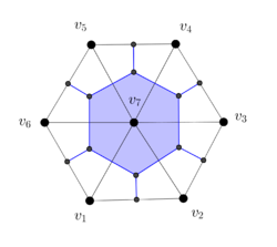
Observe the deformation of the blue-colored dual cell in Figure 19(a) as the vertex is moved to make the triangle non-well-centered in Figure 19(b) and the vertex is moved to make the triangle non-well-centered in Figure 19(c).
|
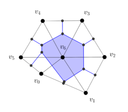
|
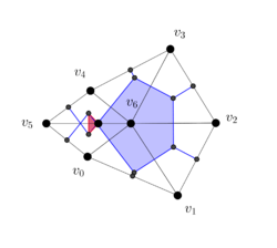
|
| (a) | (b) | (c) |
| Figure 19. Deformation of a 2-dimensional dual cell as the hexagonal region is deformed | ||
We have colored in red the part of the dual cell in Figure 16(c) that must have the opposite orientation of the blue-colored part. Similar considerations apply to the edges.
4.3. Brief digression in 2D.
In 2D, there is an intuitively clear way of comparing Discrete Exterior Calculus with the Finite Element Method (FEM) and the Finite Volume Method (FVM), both with linear interpolation functions, by considering the circumcenters of the triangles.
- Since the circumcenter of an obtuse triangle lies outside the triangle, the circumcenter cannot be used as control points of an irregular mesh for FVM.
- DEC is capable of using the circumcenter of irregular meshes. While the rigidity matrix generated by DEC works in a similar fashion to that of FEM, the discretized source term generally differs.
- When the elements of the mesh are all regular (the circumcenter of every triangle is in the triangle), DEC, FEM and FVM are very similar.
5. Numerical examples
5.1 First example
Let us solve the Poisson equation in a circle of radius one under the following conditions (Figure 20):
- heat difussion constant ;
- source term ;
- Dirichlet boundary condition .
The exact solution is
|
|
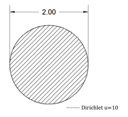
|
| Figure 20. Disk of radius one with difussion constant , subject to a heat source |
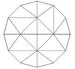
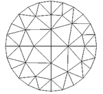
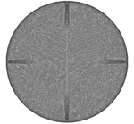
The meshes used in this example are shown in Figure 21 and vary from very coarse to very fine.
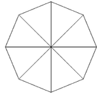
|
|
|
|
| (a) | (b) | (c) | |

|
| ||
| (d) | (e) | ||
| Figure 21. Meshes for unit disk | |||
The numerical results for the maximum temperature value () are exemplified in Table 1 where a comparison with the Finite Element Method with linear interpolation functions (FEML) is also shown. The FEML methodology that we used in the comparison can be consulted [2,12,13]. For the sake of completeness in our comparison, here we compute the flux vectors in the same way as in FEML.
| Mesh | #nodes | #elements | Max. Temp. Value | Max. Flux Magnitude | ||
| DEC | FEML | DEC | FEML | |||
| Figure (a) | 9 | 8 | 10.250 | 10.285 | 0.270 | 0.307 |
| Figure (b) | 17 | 20 | 10.250 | 10.237 | 0.388 | 0.405 |
| Figure (c) | 41 | 56 | 10.250 | 10.246 | 0.449 | 0.453 |
| Figure (d) | 713 | 1304 | 10.250 | 10.250 | 0.491 | 0.492 |
| Figure (e) | 42298 | 83346 | 10.250 | 10.250 | 0.496 | 0.496 |
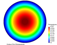
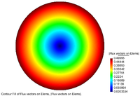
The temperature distribution and Flux magnitude fields for the finest mesh are shown in Figure 22.
|
|
| (a) | (b) |
| Figure 22. Temperature distribution and Flux magnitude fields for the finest mesh | |
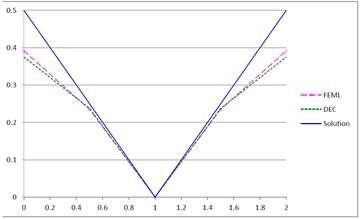
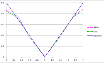
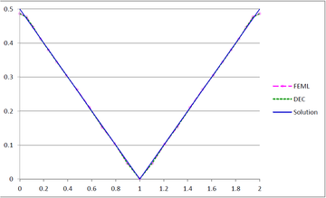
Figures 23(a), 23(b) and 23(c) show the graphs of the temperature and flux magnitude values along a diameter of the circle for the different meshes of Figures 23(b), 23(c) and 23(d) respectively.
| (a) | 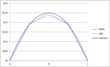
|
|
| (b) | 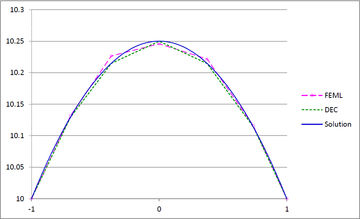
|
|
| (c) | 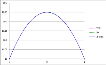
|
|
| Figure 23. Temperature and Flux magnitude graphs along a diameter of the circle for different meshes: (a) Graphs for the Mesh in Figure 23(b); (b) Graphs for the Mesh in Figure 23(c); (c) Graphs for the Mesh in Figure 23(d) | ||
As can be seen from Table 1 and Figure 20, DEC behaves very well on coarse meshes. Note that the maximum temperature values calculated with DEC matches the exact theoretical value even on coarse meshes. As expected, the results of DEC and FEML are similar for fine meshes. We would also like to point out the the computational costs of DEC and FEML are very similar.
5.2 Second example
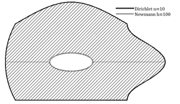
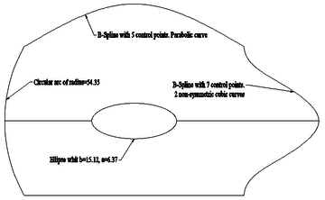
In this example, we consider a region in the plane whose boundary consists of segments of a straight line, a circle, a parabola, a cubic and an ellipse (Figure 24).
|
|
| Figure 24. Region with linear, quadratic and cubic boundary segments, together with boundary conditions | |
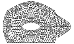
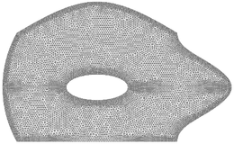
The meshes used in this example are shown in Figure 25 and vary from coarse to very fine.

|
|
|
| (a) | (b) | (c) |
| Figure 25. Three of the meshes used in the first example | ||
We set
- the source term ;
- the heat diffusion constant ;
- Newmann boundary condition along the inner elliptical boundary;
- Dirichlet boundary condition along the external boundary.
The numerical results for the maximum temperature and flux magnitude values are exemplified in Table 2.
| Mesh | #nodes | #elements | Max. Temp. Value | Max. Flux Magnitude | ||
| DEC | FEML | DEC | FEML | |||
| Figure 21(a) | 162 | 268 | 129.07 | 128.92 | 467.22 | 467.25 |
| Figure 21(b) | 678 | 1223 | 129.71 | 129.70 | 547.87 | 548.42 |
| Figure 21(c) | 9489 | 18284 | 130.00 | 130.00 | 591.58 | 591.63 |
| 27453 | 53532 | 130.01 | 130.01 | 597.37 | 597.38 | |
| 651406 | 1295960 | 130.02 | 130.02 | 602.19 | 602.19 | |
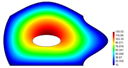
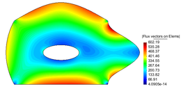
The temperature and flux-magnitude distribution fields are shown in Figure 26.
|
|
| (a) | (b) |
| Figure 26. Temperature and Flux magnitude distribution fields | |
Figure 27 shows the graphs of the temperature and the flux magnitude along a horizontal line crossing the elliptical boundary for the first two meshes.
| (a) | 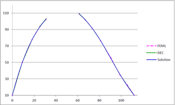
|
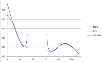
|
| (b) | 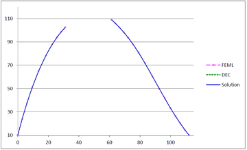
|
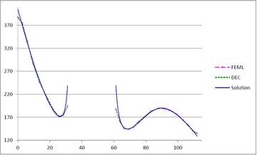
|
| Figure 27 Temperature and Flux magnitude graphs along a horizontal line crossing the elliptical boundary for the first two meshes | ||
As can be seen from Table 2 and Figure 27, the performance of DEC is very similar to that of FEML in this example. As expected, when the mesh is refined, the two methods converge to the same values.
6. Conclusions
DEC is a relatively recent discretization scheme for PDE which takes into account the geometric and analytic features of the operators and the domains involved. The main contributions of this paper are the following:
- We have presented 2D DEC in a simplified manner, avoiding references to the theory of differential forms and motivating geometrically the new operators.
- We have carried out a numerical comparison between DEC and FEML by solving the 2D Poisson equation on two cirved domains. The numerical experiments show the solutions obtained with DEC on coarse meshes are as good or better as those of FEML. On the other hand, the experiements also show numerical convergence.
- The computational cost of DEC is similar to that of FEML.
Acknowledgements
The second named author was partially supported by a grant of CONACYT, and would like to thank the International Centre for Numerical Methods in Engineering (CIMNE) and the University of Swansea for their hospitality. We gratefully acknowledge the support of NVIDIA Corporation with the donation of the Titan X Pascal GPU used for this research.
References
[1] Arnold D., Falk R., WintherR. Finite element exterior calculus: From Hodge theory to numerical stability. Bulletin of the American Mathematical Society, 47(2):281-354, 2010.
[2] Botello S., Moreles M.A., Oñate E. Módulo de aplicaciones del método de los elementos finitos para resolver la ecuación de Poisson: MEFIPOISS. Aula CIMNE-CIMAT, Septiembre 2010, ISBN 978-84-96736-95-5.
[3] Cartann E. Sur certaines expressions différentielles et le problème de Pfaff. Annales Scientifiques de l'École Normale Supérieure, Série 3, Paris, Gauthier-Villars, 16:239-332, 1899.
[4] Crane K., de Goes F., Desbrun M., Schröder P. Digital geometry processing with discrete exterior calculus. ACM SIGGRAPH 2013 Courses, ACM, 2013.
[5] Dassios I., Jivkov A.P., Abu-Muharib A., James P. A mathematical model for plasticity and damage: A discrete calculus formulation. Journal of Computational and Applied Mathematics, 312:27-38, 2017.
[6] Desbrun M., Kanso E., Tong Y. Discrete differential forms for computational modeling. In SIGGRAPH 06: ACM SIGGRAPH 2006 Courses, pp. 39–54, New York, 2006.
[7] Griebel M., Rieger C., Schier A. Upwind schemes for scalar advection-dominated problems in the discrete exterior calculus. Transport Processes at Fluidic Interfaces, Birkhäuser, Cham, pp. 145-175, 2017.
[8] Hirani A.N. Discrete exterior calculus. Diss. California Institute of Technology, 2003.
[9] Hirani A.N., Nakshatrala K.B., Chaudhry J.H. Numerical method for Darcy flow derived using Discrete Exterior Calculus. International Journal for Computational Methods in Engineering Science and Mechanics, 16(3):151-169, 2015.
[10] Hirani A.N., Kalyanaraman K., VanderZee E.B. Delaunay Hodge star. Comput. Aided Des., 45:540-544, 2013.
[11] Mohamed M.S., Hirani A.N., Samtaney R. Discrete exterior calculus discretization of incompressible Navier-Stokes equations over surface simplicial meshes. Journal of Computational Physics, 312:175-191, 2016.
[12] Oñate E. 2D Solids. Linear Triangular and Rectangular Elements (chapter 4). In Structural Analysis with the Finite Element Method. Linear Statics, Volume 1: Basis and Solids, CIMNE-Springer, pp. 117-157, Barcelona, 2009, ISBN 978-1-4020-8733-2.
[13] Zienkiewicz O.C., Taylor R.L., Zhu J.Z. Generalization of the finite element concepts. Galerkin-weighted residual and variational approaches (chapter 3). In The Finite Element Method Set (Sixth Edition), Butterworth-Heinemann, pp. 54-102, Oxford 2005, ISBN 9780750664318.
Document information
Published on 08/02/19
Accepted on 04/10/18
Submitted on 06/06/18
Volume 35, Issue 1, 2019
DOI: 10.23967/j.rimni.2018.11.003
Licence: CC BY-NC-SA license
Share this document
Keywords
claim authorship
Are you one of the authors of this document?
