m (Cinmemj moved page Draft Samper 148409403 to Flores et al 2018b) |
|||
| (24 intermediate revisions by the same user not shown) | |||
| Line 1: | Line 1: | ||
| − | + | Published in ''Comput. Methods Appl. Mech. Engrg.'', Vol. 195, pp. 5297–5315, 2006<br /> | |
| − | + | doi:10.1016/j.cma.2005.08.021 | |
| − | |||
| − | |||
| − | |||
| − | |||
| − | |||
| − | |||
| − | |||
| − | |||
| − | |||
| − | |||
| − | |||
| − | |||
| − | |||
| − | |||
| − | |||
| − | |||
| − | |||
| − | |||
==Abstract== | ==Abstract== | ||
| Line 25: | Line 7: | ||
In this paper a finite element for the non-linear analysis of two dimensional beams and axisymmetric shells is presented. The element uses classical thin shell assumptions (no transverse shear strains). The main feature of the element is that it has no rotational degrees of freedom. Curvatures are computed using geometrical information from the patch of three elements formed by the main element and the two neighbour (adjacent) elements. Special attention is devoted to non-smooth geometries and branching shells. An elastic-plastic material law is considered. Large strains are treated using a logarithmic strain measure and a through-the-thickness numerical integration of the constitutive equations. Several examples are presented including linear problems to study convergence properties, and non-linear problems for both elastic and elastic-plastic materials and large strains. | In this paper a finite element for the non-linear analysis of two dimensional beams and axisymmetric shells is presented. The element uses classical thin shell assumptions (no transverse shear strains). The main feature of the element is that it has no rotational degrees of freedom. Curvatures are computed using geometrical information from the patch of three elements formed by the main element and the two neighbour (adjacent) elements. Special attention is devoted to non-smooth geometries and branching shells. An elastic-plastic material law is considered. Large strains are treated using a logarithmic strain measure and a through-the-thickness numerical integration of the constitutive equations. Several examples are presented including linear problems to study convergence properties, and non-linear problems for both elastic and elastic-plastic materials and large strains. | ||
| − | ''' | + | '''Keywords''': finite elements, beams, axisymmetric shells, rotation-free element, large strains |
==1 Introduction== | ==1 Introduction== | ||
| − | The development of numerical techniques for shell analysis without rotational degrees of freedom has been mainly associated to the finite differences method (see for example Refs. <span id='citeF-1'></span><span id='citeF-2'></span><span id='citeF-3'></span>[[#cite-1|[1,2,3]]]. Nevertheless, the idea of developing finite elements without rotational DOFs is not new<span id='citeF-4'></span><span id='citeF-5'></span>[[#cite-4|[4,5]]] and different attempts have been reported in the last twenty years<span id='citeF-6'></span><span id='citeF-7'></span><span id='citeF-8'></span><span id='citeF-9'></span><span id='citeF-10'></span>[[#cite-6|[6,7,8,9,10]]]. Despite these attempts it is just in the last few years that reliable rotation-free elements for industrial applications have been developed<span id='citeF-11'></span><span id='citeF-12'></span><span id='citeF-13'></span><span id='citeF-14'></span>[[#cite-11|[11,12,13,14]]]. All the approximations share in common the definition of a patch (neighborhood) of elements to interpolate the geometry and the displacements. The main difference between the different approaches is the interpolation of the geometry and the theoretical basis used. One of the main aspects that remains unsolved satisfactorily is the treatment of non-smooth surfaces and specially branching shells. An adequate handling of multiple surfaces, i.e. when more than two elements share a side or edge, is mandatory if the element is to be used for the analysis of aeronautic and naval structures or frame structures typical in buildings, among others. | + | The development of numerical techniques for shell analysis without rotational degrees of freedom has been mainly associated to the finite differences method (see for example Refs. <span id='citeF-1'></span><span id='citeF-2'></span><span id='citeF-3'></span>[[#cite-1|[1,2,3]]]. Nevertheless, the idea of developing finite elements without rotational DOFs is not new <span id='citeF-4'></span><span id='citeF-5'></span>[[#cite-4|[4,5]]] and different attempts have been reported in the last twenty years <span id='citeF-6'></span><span id='citeF-7'></span><span id='citeF-8'></span><span id='citeF-9'></span><span id='citeF-10'></span>[[#cite-6|[6,7,8,9,10]]]. Despite these attempts it is just in the last few years that reliable rotation-free elements for industrial applications have been developed <span id='citeF-11'></span><span id='citeF-12'></span><span id='citeF-13'></span><span id='citeF-14'></span>[[#cite-11|[11,12,13,14]]]. All the approximations share in common the definition of a patch (neighborhood) of elements to interpolate the geometry and the displacements. The main difference between the different approaches is the interpolation of the geometry and the theoretical basis used. One of the main aspects that remains unsolved satisfactorily is the treatment of non-smooth surfaces and specially branching shells. An adequate handling of multiple surfaces, i.e. when more than two elements share a side or edge, is mandatory if the element is to be used for the analysis of aeronautic and naval structures or frame structures typical in buildings, among others. |
In this paper two-dimensional shell problems are tackled (previous work in this line can be found in Ref. <span id='citeF-15'></span><span id='citeF-16'></span>[[#cite-15|[15,16]]]) with special focus on non-smooth shells and branching lines. This work may be seen as a first step towards the development of three dimensional rotation-free shell finite elements capable of handling kinked and branching shells. | In this paper two-dimensional shell problems are tackled (previous work in this line can be found in Ref. <span id='citeF-15'></span><span id='citeF-16'></span>[[#cite-15|[15,16]]]) with special focus on non-smooth shells and branching lines. This work may be seen as a first step towards the development of three dimensional rotation-free shell finite elements capable of handling kinked and branching shells. | ||
| Line 37: | Line 19: | ||
==2 Governing equations of beams and thin two-dimensional shells== | ==2 Governing equations of beams and thin two-dimensional shells== | ||
| − | In this section a summary of the most relevant equations governing the kinematic behavior of thin shells is presented. More details can be found in the wide literature dedicated to the subject<span id='citeF-1'></span>[[#cite-1|[1]]]. In order to introduce the problem, the kinematics of two dimensional beams are considered. These equations are latter extended to axisymmetric shells. | + | In this section a summary of the most relevant equations governing the kinematic behavior of thin shells is presented. More details can be found in the wide literature dedicated to the subject <span id='citeF-1'></span>[[#cite-1|[1]]]. In order to introduce the problem, the kinematics of two dimensional beams are considered. These equations are latter extended to axisymmetric shells. |
| + | |||
| + | <div id='img-1'></div> | ||
| + | {| class="floating_imageSCP" style="text-align: center; border: 1px solid #BBB; margin: 1em auto; width: 100%;max-width: 100%;" | ||
| + | |- | ||
| + | |[[Image:Draft_Samper_148409403-fig1.png|254px|Beam geometry and notation.]] | ||
| + | |- style="text-align: center; font-size: 75%;" | ||
| + | | colspan="1" | '''Figure 1:''' Beam geometry and notation. | ||
| + | |} | ||
| + | |||
===2.1 Euler-Bernoulli beams=== | ===2.1 Euler-Bernoulli beams=== | ||
| Line 460: | Line 451: | ||
where <math display="inline">N^{I}\left( \xi \right) </math> are the standard linear Lagrangian polynomials (shape functions) defined over the interval <math display="inline">\left[ 0,1\right] </math>. This allows the evaluation of middle surface stretches and the hoop curvature but it is not enough for the computation of the in-plane curvature <math display="inline">\kappa _{s}</math>. The later is computed resorting to the geometry of the surrounding elements leading to an assumed strain approach as shown below. | where <math display="inline">N^{I}\left( \xi \right) </math> are the standard linear Lagrangian polynomials (shape functions) defined over the interval <math display="inline">\left[ 0,1\right] </math>. This allows the evaluation of middle surface stretches and the hoop curvature but it is not enough for the computation of the in-plane curvature <math display="inline">\kappa _{s}</math>. The later is computed resorting to the geometry of the surrounding elements leading to an assumed strain approach as shown below. | ||
| + | |||
| + | <div id='img-2'></div> | ||
| + | {| class="floating_imageSCP" style="text-align: center; border: 1px solid #BBB; margin: 1em auto; width: 100%;max-width: 100%;" | ||
| + | |- | ||
| + | |[[Image:Draft_Samper_148409403-fig2.png|500px|Two-node element.]] | ||
| + | |- style="text-align: center; font-size: 75%;" | ||
| + | | colspan="1" | '''Figure 2:''' Two-node element. | ||
| + | |} | ||
| + | |||
===3.1 Axial strain=== | ===3.1 Axial strain=== | ||
| Line 576: | Line 576: | ||
{| style="text-align: left; margin:auto;width: 100%;" | {| style="text-align: left; margin:auto;width: 100%;" | ||
|- | |- | ||
| − | | style="text-align: center;" | <math>\hat{E}_{\theta }=\frac{1}{2}\left[ \left( \lambda _{\theta }\right) ^{2}-1\right] =\frac{1}{2}\left\{ \frac{\left( N^{1}\varphi_{1}^{1}+N^{2}\varphi_{1}^{2}\right)^{2}}{\left( N^{ | + | | style="text-align: center;" | <math>\hat{E}_{\theta }=\frac{1}{2}\left[ \left( \lambda _{\theta }\right) ^{2}-1\right] =\frac{1}{2}\left\{ \frac{\left( N^{1}\varphi_{1}^{1}+N^{2}\varphi_{1}^{2}\right)^{2}}{\left( N^{1o}\varphi_{1}^{1}+N^{2o}\varphi_{1}^{2}\right)^{2}}-1\right\} </math> |
|} | |} | ||
| style="width: 5px;text-align: right;white-space: nowrap;" | (39) | | style="width: 5px;text-align: right;white-space: nowrap;" | (39) | ||
| Line 598: | Line 598: | ||
{| style="text-align: left; margin:auto;width: 100%;" | {| style="text-align: left; margin:auto;width: 100%;" | ||
|- | |- | ||
| − | | style="text-align: center;" | <math>\delta \hat{E}_{\theta } =\lambda _{\theta } \delta \lambda _{\theta }=\lambda _{\theta }\frac{N^{1}\delta u_{1}^{1}+N^{2}\delta u_{1}^{2}}{N^{ | + | | style="text-align: center;" | <math>\delta \hat{E}_{\theta } =\lambda _{\theta } \delta \lambda _{\theta }=\lambda _{\theta }\frac{N^{1}\delta u_{1}^{1}+N^{2}\delta u_{1}^{2}}{N^{1o}\varphi _{1}^{1}+N^{2o}\varphi _{1}^{2}}</math> |
| style="width: 5px;text-align: right;white-space: nowrap;" | (41) | | style="width: 5px;text-align: right;white-space: nowrap;" | (41) | ||
|- | |- | ||
| − | | style="text-align: center;" | <math> =\frac{\lambda _{\theta }}{N^{ | + | | style="text-align: center;" | <math> =\frac{\lambda _{\theta }}{N^{1o}\varphi _{1}^{1}+N^{2o}\varphi _{1}^{2}}\left[ N^{1},0,N^{2},0\right] \left[ \begin{array}{c}\delta u_{1}^{1}\\ \delta u_{2}^{1}\\ \delta u_{1}^{2}\\ \delta u_{2}^{2}\end{array} \right] =\underset{1\times{4}}{\mathbf{B}_{m\theta }} \underset{4\times 1}{\delta \mathbf{u}^{e}}</math> |
| − | | style="width: 5px;text-align: right;white-space: nowrap;" | ( | + | | style="width: 5px;text-align: right;white-space: nowrap;" | (42) |
|} | |} | ||
|} | |} | ||
| Line 611: | Line 611: | ||
{| style="text-align: left; margin:auto;width: 100%;" | {| style="text-align: left; margin:auto;width: 100%;" | ||
|- | |- | ||
| − | | style="text-align: center;" | <math>\delta \chi _{\theta } =\frac{\left( N^{1}\delta u_{1}^{1}+N^{2}\delta u_{1}^{2}\right) \left( -\sin \alpha \right) -\left( N^{1}\varphi _{1}^{1}+N^{2}\varphi _{1}^{2}\right) \cos \alpha \left( \mathbf{n}\cdot \delta \mathbf{t}\right) }{\left( N^{ | + | | style="text-align: center;" | <math>\delta \chi _{\theta } =\frac{\left( N^{1}\delta u_{1}^{1}+N^{2}\delta u_{1}^{2}\right) \left( -\sin \alpha \right) -\left( N^{1}\varphi _{1}^{1}+N^{2}\varphi _{1}^{2}\right) \cos \alpha \left( \mathbf{n}\cdot \delta \mathbf{t}\right) }{\left( N^{1o}\varphi _{1}^{1}+N^{2o}\varphi _{1}^{2}\right) ^{2}}</math> |
|- | |- | ||
| − | | style="text-align: center;" | <math> =-\frac{\sin \alpha \left( N^{1}\delta u_{1}^{1}+N^{2}\delta u_{1}^{2}\right) +\left( N^{1}\varphi _{1}^{1}+N^{2}\varphi _{1}^{2}\right) \cos \alpha \left( \mathbf{n}\cdot \dfrac{\delta \mathbf{\varphi }^{2}-\delta \mathbf{\varphi }^{1}}{L}\right) }{\left( N^{ | + | | style="text-align: center;" | <math> =-\frac{\sin \alpha \left( N^{1}\delta u_{1}^{1}+N^{2}\delta u_{1}^{2}\right) +\left( N^{1}\varphi _{1}^{1}+N^{2}\varphi _{1}^{2}\right) \cos \alpha \left( \mathbf{n}\cdot \dfrac{\delta \mathbf{\varphi }^{2}-\delta \mathbf{\varphi }^{1}}{L}\right) }{\left( N^{1o}\varphi _{1}^{1}+N^{2o}\varphi _{1}^{2}\right) ^{2}}=\underset{1\times{4}}{\mathbf{B}_{b\theta }} \underset{4\times{1}}{\delta \mathbf{u}^{e}}</math> |
|} | |} | ||
| − | | style="width: 5px;text-align: right;white-space: nowrap;" | ( | + | | style="width: 5px;text-align: right;white-space: nowrap;" | (43) |
|} | |} | ||
| Line 630: | Line 630: | ||
|- | |- | ||
| style="text-align: center;" | <math>\bar{\kappa }_{s}\left( s\right) =\left( 1-\frac{s}{^{o}L}\right) \kappa _{s}^{\left( 1\right) }+\frac{s}{^{o}L}\kappa _{s}^{\left( 2\right) }</math> | | style="text-align: center;" | <math>\bar{\kappa }_{s}\left( s\right) =\left( 1-\frac{s}{^{o}L}\right) \kappa _{s}^{\left( 1\right) }+\frac{s}{^{o}L}\kappa _{s}^{\left( 2\right) }</math> | ||
| − | | style="width: 5px;text-align: right;white-space: nowrap;" | ( | + | | style="width: 5px;text-align: right;white-space: nowrap;" | (44) |
|- | |- | ||
| style="text-align: center;" | <math> =-N^{1}\lambda _{s}^{\left( 1\right) }\alpha _{^{\prime }s}^{\left( 1\right) }-N^{2}\lambda _{s}^{\left( 2\right) }\alpha _{^{\prime }s}^{\left( 2\right) } </math> | | style="text-align: center;" | <math> =-N^{1}\lambda _{s}^{\left( 1\right) }\alpha _{^{\prime }s}^{\left( 1\right) }-N^{2}\lambda _{s}^{\left( 2\right) }\alpha _{^{\prime }s}^{\left( 2\right) } </math> | ||
| − | | style="width: 5px;text-align: right;white-space: nowrap;" | ( | + | | style="width: 5px;text-align: right;white-space: nowrap;" | (45) |
|} | |} | ||
|} | |} | ||
| Line 640: | Line 640: | ||
As in other rotation-free element, for the computation of the curvatures, the position of the nodes in the adjacent element is considered. In this case a patch of three elements (see Figure [[#img-3|3]]) is involved. There are different options for the computation of the curvatures at each element node. Initially an approximation adequate for smooth and homogeneous beam is defined. This approximation is latter modified to deal with more general geometries, including non-smooth and branching lines. | As in other rotation-free element, for the computation of the curvatures, the position of the nodes in the adjacent element is considered. In this case a patch of three elements (see Figure [[#img-3|3]]) is involved. There are different options for the computation of the curvatures at each element node. Initially an approximation adequate for smooth and homogeneous beam is defined. This approximation is latter modified to deal with more general geometries, including non-smooth and branching lines. | ||
| + | |||
| + | <div id='img-3'></div> | ||
| + | {| class="floating_imageSCP" style="text-align: center; border: 1px solid #BBB; margin: 1em auto; width: 100%;max-width: 100%;" | ||
| + | |- | ||
| + | |[[Image:Draft_Samper_148409403-fig3.png|400px|Patch of elements used for the evaluation of the curvature.]] | ||
| + | |- style="text-align: center; font-size: 75%;" | ||
| + | | colspan="1" | '''Figure 3:''' Patch of elements used for the evaluation of the curvature. | ||
| + | |} | ||
| + | |||
For the initial approximation of ([[#eq-9|9]]) the following (finite differences) computations can be used at each node: | For the initial approximation of ([[#eq-9|9]]) the following (finite differences) computations can be used at each node: | ||
| Line 673: | Line 682: | ||
|- | |- | ||
| style="text-align: center;" | <math>\kappa _{s}^{\left( 1\right) } =\frac{\lambda _{sl}+\lambda _{s}}{2}\frac{2\phi ^{1}}{^{o}L_{l}+ ^{o}L}=\frac{\lambda _{sl}+\lambda _{s}}{^{o}L_{l}+ ^{o}L}\phi ^{1}</math> | | style="text-align: center;" | <math>\kappa _{s}^{\left( 1\right) } =\frac{\lambda _{sl}+\lambda _{s}}{2}\frac{2\phi ^{1}}{^{o}L_{l}+ ^{o}L}=\frac{\lambda _{sl}+\lambda _{s}}{^{o}L_{l}+ ^{o}L}\phi ^{1}</math> | ||
| − | | style="width: 5px;text-align: right;white-space: nowrap;" | ( | + | | style="width: 5px;text-align: right;white-space: nowrap;" | (46.a) |
|- | |- | ||
| style="text-align: center;" | <math> \kappa _{s}^{\left( 2\right) } =\frac{\lambda _{s}+\lambda _{sr}}{^{o}L+ ^{o}L_{r}}\phi ^{2}</math> | | style="text-align: center;" | <math> \kappa _{s}^{\left( 2\right) } =\frac{\lambda _{s}+\lambda _{sr}}{^{o}L+ ^{o}L_{r}}\phi ^{2}</math> | ||
| − | | style="width: 5px;text-align: right;white-space: nowrap;" | ( | + | | style="width: 5px;text-align: right;white-space: nowrap;" | (46.b) |
|} | |} | ||
|} | |} | ||
| − | In Eqs.([[#3.3 Evaluation of the in-plane curvature| | + | In Eqs.([[#3.3 Evaluation of the in-plane curvature|46]]) indexes <math display="inline">l</math> and <math display="inline">r</math> denote the left and right end nodes in the three elements patch (see Figure [[#img-3|3]]). Also <math display="inline">^{o}L_{r}</math> and <math display="inline">^{o}L_{l}</math> are the initial lengths of the elements respectively located at the right and the left of the central element in the patch. |
For future reference the following angles must be identified | For future reference the following angles must be identified | ||
| Line 710: | Line 719: | ||
For the initially horizontal elements of Figure [[#img-3|3]] the angle <math display="inline">\alpha </math> is also the rotation <math display="inline">\beta </math> of the element. While the relative angle <math display="inline">\phi ^{1}</math> between the tangent vector of the central element (<math display="inline">\mathbf{t}</math>) and the tangent vector of the left element (<math display="inline">\mathbf{t}_{l}</math>) measured from <math display="inline">\mathbf{t}</math> to <math display="inline">\mathbf{t}_{l}</math> counter-clockwise (see Figure [[#img-4|4]]) is also the relative rotation <math display="inline">\beta{-\beta}_{l}</math>. Similarly <math display="inline">\phi ^{2}</math> is the angle between the tangent vector of the central element (<math display="inline">\mathbf{t}</math>) and the tangent vector of the right element (<math display="inline">\mathbf{t}_{r}</math>) measured from <math display="inline">\mathbf{t}_{r}</math> to <math display="inline">\mathbf{t}</math> counter-clockwise. | For the initially horizontal elements of Figure [[#img-3|3]] the angle <math display="inline">\alpha </math> is also the rotation <math display="inline">\beta </math> of the element. While the relative angle <math display="inline">\phi ^{1}</math> between the tangent vector of the central element (<math display="inline">\mathbf{t}</math>) and the tangent vector of the left element (<math display="inline">\mathbf{t}_{l}</math>) measured from <math display="inline">\mathbf{t}</math> to <math display="inline">\mathbf{t}_{l}</math> counter-clockwise (see Figure [[#img-4|4]]) is also the relative rotation <math display="inline">\beta{-\beta}_{l}</math>. Similarly <math display="inline">\phi ^{2}</math> is the angle between the tangent vector of the central element (<math display="inline">\mathbf{t}</math>) and the tangent vector of the right element (<math display="inline">\mathbf{t}_{r}</math>) measured from <math display="inline">\mathbf{t}_{r}</math> to <math display="inline">\mathbf{t}</math> counter-clockwise. | ||
| − | The approximation above leading to expressions ([[#3.3 Evaluation of the in-plane curvature| | + | <div id='img-4'></div> |
| + | {| class="floating_imageSCP" style="text-align: center; border: 1px solid #BBB; margin: 1em auto; width: 100%;max-width: 100%;" | ||
| + | |- | ||
| + | |[[Image:Draft_Samper_148409403-fig4.png|500px|Change of angle between elements.]] | ||
| + | |- style="text-align: center; font-size: 75%;" | ||
| + | | colspan="1" | '''Figure 4:''' Change of angle between elements. | ||
| + | |} | ||
| + | |||
| + | |||
| + | The approximation above leading to expressions ([[#3.3 Evaluation of the in-plane curvature|46]]) define a unique curvature value at each node, independently of the element from where it is computed. This represents a drawback for nonhomogeneous beams/shells, i.e. when there are changes in the material or in the transverse section properties of the beam/shell. Then at the intersection node <math display="inline">n</math> of the two elements <math display="inline">i</math> and <math display="inline">j</math> of Figure [[#img-4|4]] with different bending stiffness (<math display="inline">EI</math>), equilibrium can not be fulfilled at the node as | ||
<span id="eq-50"></span> | <span id="eq-50"></span> | ||
| Line 720: | Line 738: | ||
| style="text-align: center;" | <math>M_{si}^{\left( n\right) }=\left( EI\right) _{i}\kappa _{si}^{\left( n\right) }\neq \left( EI\right) _{j}\kappa _{sj}^{\left( n\right) }=M_{sj}^{\left( n\right) } </math> | | style="text-align: center;" | <math>M_{si}^{\left( n\right) }=\left( EI\right) _{i}\kappa _{si}^{\left( n\right) }\neq \left( EI\right) _{j}\kappa _{sj}^{\left( n\right) }=M_{sj}^{\left( n\right) } </math> | ||
|} | |} | ||
| − | | style="width: 5px;text-align: right;white-space: nowrap;" | ( | + | | style="width: 5px;text-align: right;white-space: nowrap;" | (47) |
|} | |} | ||
| Line 735: | Line 753: | ||
| style="text-align: center;" | <math>\kappa _{si}^{\left( n\right) }=\frac{\lambda _{si}}{^{o}L_{i}}\gamma _{i}^{\left( n\right) } </math> | | style="text-align: center;" | <math>\kappa _{si}^{\left( n\right) }=\frac{\lambda _{si}}{^{o}L_{i}}\gamma _{i}^{\left( n\right) } </math> | ||
|} | |} | ||
| − | | style="width: 5px;text-align: right;white-space: nowrap;" | ( | + | | style="width: 5px;text-align: right;white-space: nowrap;" | (48) |
|} | |} | ||
| Line 746: | Line 764: | ||
| style="text-align: center;" | <math>\kappa _{sj}^{\left( n\right) }=\frac{\lambda _{sj}}{^{o}L_{j}}\gamma _{j}^{\left( n\right) } </math> | | style="text-align: center;" | <math>\kappa _{sj}^{\left( n\right) }=\frac{\lambda _{sj}}{^{o}L_{j}}\gamma _{j}^{\left( n\right) } </math> | ||
|} | |} | ||
| − | | style="width: 5px;text-align: right;white-space: nowrap;" | ( | + | | style="width: 5px;text-align: right;white-space: nowrap;" | (49) |
|} | |} | ||
| Line 757: | Line 775: | ||
|- | |- | ||
| style="text-align: center;" | <math>\gamma _{i}^{\left( n\right) } =2\left( \beta _{i}-\bar{\beta }^{n}\right) </math> | | style="text-align: center;" | <math>\gamma _{i}^{\left( n\right) } =2\left( \beta _{i}-\bar{\beta }^{n}\right) </math> | ||
| − | | style="width: 5px;text-align: right;white-space: nowrap;" | ( | + | | style="width: 5px;text-align: right;white-space: nowrap;" | (50.a) |
|- | |- | ||
| style="text-align: center;" | <math> \gamma _{j}^{\left( n\right) } =2\left( \bar{\beta }^{n}-\beta _{j}\right) </math> | | style="text-align: center;" | <math> \gamma _{j}^{\left( n\right) } =2\left( \bar{\beta }^{n}-\beta _{j}\right) </math> | ||
| − | | style="width: 5px;text-align: right;white-space: nowrap;" | ( | + | | style="width: 5px;text-align: right;white-space: nowrap;" | (50.b) |
|} | |} | ||
|} | |} | ||
| Line 774: | Line 792: | ||
| style="text-align: center;" | <math>\gamma _{i}^{\left( n\right) }+\gamma _{j}^{\left( n\right) }=2\left( \beta _{i}-\beta _{j}\right) =2\phi ^{n} </math> | | style="text-align: center;" | <math>\gamma _{i}^{\left( n\right) }+\gamma _{j}^{\left( n\right) }=2\left( \beta _{i}-\beta _{j}\right) =2\phi ^{n} </math> | ||
|} | |} | ||
| − | | style="width: 5px;text-align: right;white-space: nowrap;" | ( | + | | style="width: 5px;text-align: right;white-space: nowrap;" | (51) |
|} | |} | ||
| Line 788: | Line 806: | ||
|- | |- | ||
| style="text-align: center;" | <math>\left( \frac{EI}{^{o}L}\right) _{i}\gamma _{i}^{\left( n\right) } =\left( \frac{EI}{^{o}L}\right) _{j}\gamma _{j}^{\left( n\right) }</math> | | style="text-align: center;" | <math>\left( \frac{EI}{^{o}L}\right) _{i}\gamma _{i}^{\left( n\right) } =\left( \frac{EI}{^{o}L}\right) _{j}\gamma _{j}^{\left( n\right) }</math> | ||
| − | | style="width: 5px;text-align: right;white-space: nowrap;" | ( | + | | style="width: 5px;text-align: right;white-space: nowrap;" | (52) |
|- | |- | ||
| style="text-align: center;" | <math> R_{i}\gamma _{i}^{\left( n\right) } =R_{j}\gamma _{j}^{\left( n\right) } \hbox{ with} R_{k}=\left( {\frac{EI}{^{o}L}}\right) _{k}\quad k=i,j </math> | | style="text-align: center;" | <math> R_{i}\gamma _{i}^{\left( n\right) } =R_{j}\gamma _{j}^{\left( n\right) } \hbox{ with} R_{k}=\left( {\frac{EI}{^{o}L}}\right) _{k}\quad k=i,j </math> | ||
| − | | style="width: 5px;text-align: right;white-space: nowrap;" | ( | + | | style="width: 5px;text-align: right;white-space: nowrap;" | (53) |
|} | |} | ||
|} | |} | ||
| − | Replacing Eq.([[#eq-54| | + | Replacing Eq.([[#eq-54|51]]) in the equilibrium relation ([[#eq-56|53]]) the values of <math display="inline">\gamma _{k}^{\left( n\right) }</math> can be expressed in terms of the relative angle <math display="inline">\phi ^{n}</math> and the stiffness measures (<math display="inline">R_{k}</math>) |
{| class="formulaSCP" style="width: 100%; text-align: left;" | {| class="formulaSCP" style="width: 100%; text-align: left;" | ||
| Line 803: | Line 821: | ||
|- | |- | ||
| style="text-align: center;" | <math>\gamma _{i}^{\left( n\right) } =\frac{2R_{j}}{R_{i}+R_{j}}\left( \beta _{i}-\beta _{j}\right) =c_{j}\phi ^{n}</math> | | style="text-align: center;" | <math>\gamma _{i}^{\left( n\right) } =\frac{2R_{j}}{R_{i}+R_{j}}\left( \beta _{i}-\beta _{j}\right) =c_{j}\phi ^{n}</math> | ||
| − | | style="width: 5px;text-align: right;white-space: nowrap;" | ( | + | | style="width: 5px;text-align: right;white-space: nowrap;" | (54.a) |
|- | |- | ||
| style="text-align: center;" | <math> \gamma _{j}^{\left( n\right) } =\frac{2R_{i}}{R_{i}+R_{j}}\left( \beta _{i}-\beta _{j}\right) =c_{i}\phi ^{n}</math> | | style="text-align: center;" | <math> \gamma _{j}^{\left( n\right) } =\frac{2R_{i}}{R_{i}+R_{j}}\left( \beta _{i}-\beta _{j}\right) =c_{i}\phi ^{n}</math> | ||
| − | | style="width: 5px;text-align: right;white-space: nowrap;" | ( | + | | style="width: 5px;text-align: right;white-space: nowrap;" | (54.b) |
|} | |} | ||
|} | |} | ||
| Line 820: | Line 838: | ||
| style="text-align: center;" | <math>\gamma _{j}^{\left( n\right) }-\gamma _{i}^{\left( n\right) }=4\bar{\beta }^{n}-2\left( \beta _{i}+\beta _{j}\right) </math> | | style="text-align: center;" | <math>\gamma _{j}^{\left( n\right) }-\gamma _{i}^{\left( n\right) }=4\bar{\beta }^{n}-2\left( \beta _{i}+\beta _{j}\right) </math> | ||
|} | |} | ||
| − | | style="width: 5px;text-align: right;white-space: nowrap;" | ( | + | | style="width: 5px;text-align: right;white-space: nowrap;" | (55) |
|} | |} | ||
| − | replacing Eq.([[#3.3 Evaluation of the in-plane curvature| | + | replacing Eq.([[#3.3 Evaluation of the in-plane curvature|54]]) into ([[#eq-58|55]]) it allows to define the rotation of the node <math display="inline">\bar{\beta }^{n}</math> as: |
{| class="formulaSCP" style="width: 100%; text-align: left;" | {| class="formulaSCP" style="width: 100%; text-align: left;" | ||
| Line 832: | Line 850: | ||
| style="text-align: center;" | <math>\bar{\beta }^{n}=\frac{1}{R_{i}+R_{j}}\left( R_{i}\beta _{i}+R_{j}\beta _{j}\right) </math> | | style="text-align: center;" | <math>\bar{\beta }^{n}=\frac{1}{R_{i}+R_{j}}\left( R_{i}\beta _{i}+R_{j}\beta _{j}\right) </math> | ||
|} | |} | ||
| − | | style="width: 5px;text-align: right;white-space: nowrap;" | ( | + | | style="width: 5px;text-align: right;white-space: nowrap;" | (56) |
|} | |} | ||
| − | Then, the rotation of the node <math display="inline">\bar{\beta }^{n}</math> can be computed as the average of the rotation of the two adjacent elements weighted by their respective stiffness measure (<math display="inline">R_{k}</math>). Above expressions ([[#3.3 Evaluation of the in-plane curvature| | + | Then, the rotation of the node <math display="inline">\bar{\beta }^{n}</math> can be computed as the average of the rotation of the two adjacent elements weighted by their respective stiffness measure (<math display="inline">R_{k}</math>). Above expressions ([[#3.3 Evaluation of the in-plane curvature|54]]) allow to compute the curvature at any point of the element by Eq.([[#eq-48|45]]). |
The variation of the curvature at an arbitrary point can be expressed as: | The variation of the curvature at an arbitrary point can be expressed as: | ||
| Line 847: | Line 865: | ||
| style="text-align: center;" | <math>\delta \bar{\kappa }_{s}=\left[ N^{1}\delta \kappa _{s}^{\left( 1\right) }+N^{2}\delta \kappa _{s}^{\left( 2\right) }\right] </math> | | style="text-align: center;" | <math>\delta \bar{\kappa }_{s}=\left[ N^{1}\delta \kappa _{s}^{\left( 1\right) }+N^{2}\delta \kappa _{s}^{\left( 2\right) }\right] </math> | ||
|} | |} | ||
| − | | style="width: 5px;text-align: right;white-space: nowrap;" | ( | + | | style="width: 5px;text-align: right;white-space: nowrap;" | (57) |
|} | |} | ||
| − | From Eq. ([[#eq-52| | + | From Eq. ([[#eq-52|49]]) the variation of the nodal curvature is composed of two parts |
<span id="eq-61"></span> | <span id="eq-61"></span> | ||
| Line 860: | Line 878: | ||
| style="text-align: center;" | <math>\delta \kappa _{s}^{(n)}=\delta \left( {\frac{\lambda _{s}}{^{o}L}}\gamma ^{\left( n\right) }\right) ={\frac{\gamma ^{\left( n\right) }}{^{o}L}}\delta \lambda _{s}+{\frac{\lambda _{s}}{^{o}L}}\delta \gamma ^{\left( n\right) } </math> | | style="text-align: center;" | <math>\delta \kappa _{s}^{(n)}=\delta \left( {\frac{\lambda _{s}}{^{o}L}}\gamma ^{\left( n\right) }\right) ={\frac{\gamma ^{\left( n\right) }}{^{o}L}}\delta \lambda _{s}+{\frac{\lambda _{s}}{^{o}L}}\delta \gamma ^{\left( n\right) } </math> | ||
|} | |} | ||
| − | | style="width: 5px;text-align: right;white-space: nowrap;" | ( | + | | style="width: 5px;text-align: right;white-space: nowrap;" | (58) |
|} | |} | ||
| − | The variations <math display="inline">\delta \lambda _{s}</math> can be obtained as in ([[#3.1 Axial strain| | + | The variations <math display="inline">\delta \lambda _{s}</math> can be obtained as in ([[#3.1 Axial strain|37]]c) |
<span id="eq-62"></span> | <span id="eq-62"></span> | ||
| Line 873: | Line 891: | ||
| style="text-align: center;" | <math>\delta \lambda _{s}=\frac{\mathbf{t}\cdot \left( \delta \mathbf{\varphi }^{2}-\delta \mathbf{\varphi }^{1}\right) }{^{o}L} </math> | | style="text-align: center;" | <math>\delta \lambda _{s}=\frac{\mathbf{t}\cdot \left( \delta \mathbf{\varphi }^{2}-\delta \mathbf{\varphi }^{1}\right) }{^{o}L} </math> | ||
|} | |} | ||
| − | | style="width: 5px;text-align: right;white-space: nowrap;" | ( | + | | style="width: 5px;text-align: right;white-space: nowrap;" | (59) |
|} | |} | ||
| − | While the variation <math display="inline">\delta \gamma ^{\left( n\right) }</math> can be obtained from ([[#3.3 Evaluation of the in-plane curvature| | + | While the variation <math display="inline">\delta \gamma ^{\left( n\right) }</math> can be obtained from ([[#3.3 Evaluation of the in-plane curvature|54]]) as (see Appendix): |
{| class="formulaSCP" style="width: 100%; text-align: left;" | {| class="formulaSCP" style="width: 100%; text-align: left;" | ||
| Line 884: | Line 902: | ||
|- | |- | ||
| style="text-align: center;" | <math>\delta \gamma ^{\left( 1\right) } =\frac{2R_{l}}{R+R_{l}}\delta \left( \beta _{l}-\beta \right) =c_{l}\delta \phi ^{1}=c_{l}\left[ \frac{\delta \mathbf{\varphi }^{1}-\delta \mathbf{\varphi }^{2}}{L}\cdot \mathbf{n}+\frac{\delta \mathbf{\varphi }^{1}-\delta \mathbf{\varphi }^{l}}{L}\cdot \mathbf{n}_{l}\right]</math> | | style="text-align: center;" | <math>\delta \gamma ^{\left( 1\right) } =\frac{2R_{l}}{R+R_{l}}\delta \left( \beta _{l}-\beta \right) =c_{l}\delta \phi ^{1}=c_{l}\left[ \frac{\delta \mathbf{\varphi }^{1}-\delta \mathbf{\varphi }^{2}}{L}\cdot \mathbf{n}+\frac{\delta \mathbf{\varphi }^{1}-\delta \mathbf{\varphi }^{l}}{L}\cdot \mathbf{n}_{l}\right]</math> | ||
| − | | style="width: 5px;text-align: right;white-space: nowrap;" | ( | + | | style="width: 5px;text-align: right;white-space: nowrap;" | (60.a) |
|- | |- | ||
| style="text-align: center;" | <math> \delta \gamma ^{\left( 2\right) } =\frac{2R_{r}}{R+R_{r}}\delta \left( \beta{-\beta}_{r}\right) =c_{r}\delta \phi ^{2}=c_{r}\left[ \frac{\delta \mathbf{\varphi }^{2}-\delta \mathbf{\varphi }^{1}}{L}\cdot \mathbf{n}+\frac{\delta \mathbf{\varphi }^{r}-\delta \mathbf{\varphi }^{2}}{L_{r}}\cdot \mathbf{n}_{r}\right] </math> | | style="text-align: center;" | <math> \delta \gamma ^{\left( 2\right) } =\frac{2R_{r}}{R+R_{r}}\delta \left( \beta{-\beta}_{r}\right) =c_{r}\delta \phi ^{2}=c_{r}\left[ \frac{\delta \mathbf{\varphi }^{2}-\delta \mathbf{\varphi }^{1}}{L}\cdot \mathbf{n}+\frac{\delta \mathbf{\varphi }^{r}-\delta \mathbf{\varphi }^{2}}{L_{r}}\cdot \mathbf{n}_{r}\right] </math> | ||
| − | | style="width: 5px;text-align: right;white-space: nowrap;" | ( | + | | style="width: 5px;text-align: right;white-space: nowrap;" | (60.b) |
|} | |} | ||
|} | |} | ||
| − | Substituting Eqs. ([[#eq-62| | + | Substituting Eqs. ([[#eq-62|59]]) and ([[#3.3 Evaluation of the in-plane curvature|60]]) into ([[#eq-61|58]]) gives |
<span id="eq-64"></span> | <span id="eq-64"></span> | ||
| Line 900: | Line 918: | ||
|- | |- | ||
| style="text-align: center;" | <math>\delta \kappa _{s}^{\left( 1\right) } =\frac{1}{^{o}L}\left[ \gamma ^{\left( 1\right) }\frac{\delta \mathbf{\varphi }^{2}-\delta \mathbf{\varphi }^{1}}{^{o}L}\cdot \mathbf{t}+\lambda _{s} c_{l}\left( \frac{\delta \mathbf{\varphi }^{1}-\delta \mathbf{\varphi }^{l}}{L_{l}}\cdot \mathbf{n}_{l}+\frac{\delta \mathbf{\varphi }^{1}-\delta \mathbf{\varphi }^{2}}{L}\cdot \mathbf{n}\right) \right]</math> | | style="text-align: center;" | <math>\delta \kappa _{s}^{\left( 1\right) } =\frac{1}{^{o}L}\left[ \gamma ^{\left( 1\right) }\frac{\delta \mathbf{\varphi }^{2}-\delta \mathbf{\varphi }^{1}}{^{o}L}\cdot \mathbf{t}+\lambda _{s} c_{l}\left( \frac{\delta \mathbf{\varphi }^{1}-\delta \mathbf{\varphi }^{l}}{L_{l}}\cdot \mathbf{n}_{l}+\frac{\delta \mathbf{\varphi }^{1}-\delta \mathbf{\varphi }^{2}}{L}\cdot \mathbf{n}\right) \right]</math> | ||
| − | | style="width: 5px;text-align: right;white-space: nowrap;" | ( | + | | style="width: 5px;text-align: right;white-space: nowrap;" | (61) |
|- | |- | ||
| style="text-align: center;" | <math> =\frac{1}{^{o}L}\left\{ -\frac{\lambda _{s} c_{l}}{L_{l}}\mathbf{n}_{l}, \left[ \lambda _{s} c_{l}\left( \frac{\mathbf{n}_{l}}{L_{l}}+\frac{\mathbf{n}}{L}\right) -\frac{\gamma ^{\left( 1\right) }}{^{o}L}\mathbf{t}\right] , \left[ \frac{\gamma ^{\left( 1\right) }}{^{o}L}\mathbf{t}-\frac{\lambda _{s} c_{l}}{L}\mathbf{n}\right] ,0\right\} \left[ \begin{array}{c}[c]{c}\delta \mathbf{u}^{l}\\ \delta \mathbf{u}^{1}\\ \delta \mathbf{u}^{2}\\ \delta \mathbf{u}^{r}\end{array} \right]</math> | | style="text-align: center;" | <math> =\frac{1}{^{o}L}\left\{ -\frac{\lambda _{s} c_{l}}{L_{l}}\mathbf{n}_{l}, \left[ \lambda _{s} c_{l}\left( \frac{\mathbf{n}_{l}}{L_{l}}+\frac{\mathbf{n}}{L}\right) -\frac{\gamma ^{\left( 1\right) }}{^{o}L}\mathbf{t}\right] , \left[ \frac{\gamma ^{\left( 1\right) }}{^{o}L}\mathbf{t}-\frac{\lambda _{s} c_{l}}{L}\mathbf{n}\right] ,0\right\} \left[ \begin{array}{c}[c]{c}\delta \mathbf{u}^{l}\\ \delta \mathbf{u}^{1}\\ \delta \mathbf{u}^{2}\\ \delta \mathbf{u}^{r}\end{array} \right]</math> | ||
| − | | style="width: 5px;text-align: right;white-space: nowrap;" | ( | + | | style="width: 5px;text-align: right;white-space: nowrap;" | (62) |
|- | |- | ||
| style="text-align: center;" | <math> =\mathbf{B}_{bs}^{\left( 1\right) }\delta \mathbf{u}^{p}</math> | | style="text-align: center;" | <math> =\mathbf{B}_{bs}^{\left( 1\right) }\delta \mathbf{u}^{p}</math> | ||
| − | | style="width: 5px;text-align: right;white-space: nowrap;" | ( | + | | style="width: 5px;text-align: right;white-space: nowrap;" | (63) |
|} | |} | ||
|} | |} | ||
| Line 912: | Line 930: | ||
where <math display="inline">\delta \mathbf{u}^{p}</math> gathers the displacements of all the nodes in the patch (although node <math display="inline">r</math> have no contributions in the curvature at node <math display="inline">1</math>). | where <math display="inline">\delta \mathbf{u}^{p}</math> gathers the displacements of all the nodes in the patch (although node <math display="inline">r</math> have no contributions in the curvature at node <math display="inline">1</math>). | ||
| − | The variation of ([[#eq-51| | + | The variation of ([[#eq-51|48]]) is similarly obtained as: |
<span id="eq-70"></span> | <span id="eq-70"></span> | ||
| Line 921: | Line 939: | ||
|- | |- | ||
| style="text-align: center;" | <math>\delta \kappa _{s}^{\left( 2\right) } =\frac{1}{^{o}L}\left[ \gamma ^{\left( 2\right) }\frac{\delta \mathbf{\varphi }^{2}-\delta \mathbf{\varphi }^{1}}{^{o}L}\cdot \mathbf{t}+\lambda _{s} c_{r}\left( \frac{\delta \mathbf{\varphi }^{2}-\delta \mathbf{\varphi }^{1}}{L}\cdot \mathbf{n}+\frac{\delta \mathbf{\varphi }^{2}-\delta \mathbf{\varphi }^{r}}{L_{r}}\cdot \mathbf{n}_{r}\right) \right]</math> | | style="text-align: center;" | <math>\delta \kappa _{s}^{\left( 2\right) } =\frac{1}{^{o}L}\left[ \gamma ^{\left( 2\right) }\frac{\delta \mathbf{\varphi }^{2}-\delta \mathbf{\varphi }^{1}}{^{o}L}\cdot \mathbf{t}+\lambda _{s} c_{r}\left( \frac{\delta \mathbf{\varphi }^{2}-\delta \mathbf{\varphi }^{1}}{L}\cdot \mathbf{n}+\frac{\delta \mathbf{\varphi }^{2}-\delta \mathbf{\varphi }^{r}}{L_{r}}\cdot \mathbf{n}_{r}\right) \right]</math> | ||
| − | | style="width: 5px;text-align: right;white-space: nowrap;" | ( | + | | style="width: 5px;text-align: right;white-space: nowrap;" | (64) |
|- | |- | ||
| style="text-align: center;" | <math> =\frac{1}{^{o}L}\left\{ 0, \left[ \frac{\gamma ^{2}}{^{o}L}\mathbf{t}-\frac{\lambda _{s} c_{r}}{L}\mathbf{n}\right] ,\left[ \lambda _{s} c_{r}\left( \frac{\mathbf{n}_{r}}{L_{r}}+\frac{\mathbf{n}}{L}\right) -\frac{\gamma ^{\left( 2\right) }}{^{o}L}\mathbf{t}\right] , -\frac{\lambda _{s} c_{r}}{L_{r}}\mathbf{n}_{r}\right\} \left[ \begin{array}{c}[c]{c}\delta \mathbf{u}^{l}\\ \delta \mathbf{u}^{1}\\ \delta \mathbf{u}^{2}\\ \delta \mathbf{u}^{r}\end{array} \right]</math> | | style="text-align: center;" | <math> =\frac{1}{^{o}L}\left\{ 0, \left[ \frac{\gamma ^{2}}{^{o}L}\mathbf{t}-\frac{\lambda _{s} c_{r}}{L}\mathbf{n}\right] ,\left[ \lambda _{s} c_{r}\left( \frac{\mathbf{n}_{r}}{L_{r}}+\frac{\mathbf{n}}{L}\right) -\frac{\gamma ^{\left( 2\right) }}{^{o}L}\mathbf{t}\right] , -\frac{\lambda _{s} c_{r}}{L_{r}}\mathbf{n}_{r}\right\} \left[ \begin{array}{c}[c]{c}\delta \mathbf{u}^{l}\\ \delta \mathbf{u}^{1}\\ \delta \mathbf{u}^{2}\\ \delta \mathbf{u}^{r}\end{array} \right]</math> | ||
| − | | style="width: 5px;text-align: right;white-space: nowrap;" | ( | + | | style="width: 5px;text-align: right;white-space: nowrap;" | (65) |
|- | |- | ||
| style="text-align: center;" | <math> =\mathbf{B}_{bs}^{\left( 2\right) }\delta \mathbf{u}^{p}</math> | | style="text-align: center;" | <math> =\mathbf{B}_{bs}^{\left( 2\right) }\delta \mathbf{u}^{p}</math> | ||
| − | | style="width: 5px;text-align: right;white-space: nowrap;" | ( | + | | style="width: 5px;text-align: right;white-space: nowrap;" | (66) |
|} | |} | ||
|} | |} | ||
| − | Finally ([[#eq-60| | + | Finally ([[#eq-60|57]]) can be written as: |
{| class="formulaSCP" style="width: 100%; text-align: left;" | {| class="formulaSCP" style="width: 100%; text-align: left;" | ||
| Line 939: | Line 957: | ||
|- | |- | ||
| style="text-align: center;" | <math>\delta \bar{\kappa }_{s} =N^{1}\delta \kappa _{s}^{\left( 1\right) }+N^{2}\delta \kappa _{s}^{\left( 2\right) }=\left[ N^{1}\mathbf{B}_{bs}^{\left( 1\right) }+N^{2}\mathbf{B}_{bs}^{\left( 2\right) }\right] \delta \mathbf{u}^{p}</math> | | style="text-align: center;" | <math>\delta \bar{\kappa }_{s} =N^{1}\delta \kappa _{s}^{\left( 1\right) }+N^{2}\delta \kappa _{s}^{\left( 2\right) }=\left[ N^{1}\mathbf{B}_{bs}^{\left( 1\right) }+N^{2}\mathbf{B}_{bs}^{\left( 2\right) }\right] \delta \mathbf{u}^{p}</math> | ||
| − | | style="width: 5px;text-align: right;white-space: nowrap;" | ( | + | | style="width: 5px;text-align: right;white-space: nowrap;" | (67) |
|- | |- | ||
| style="text-align: center;" | <math> =\underset{1\times{8}}{\mathbf{B}_{bs}\left( s\right) } \underset {8\times{1}}{\delta \mathbf{u}^{p}}</math> | | style="text-align: center;" | <math> =\underset{1\times{8}}{\mathbf{B}_{bs}\left( s\right) } \underset {8\times{1}}{\delta \mathbf{u}^{p}}</math> | ||
| − | | style="width: 5px;text-align: right;white-space: nowrap;" | ( | + | | style="width: 5px;text-align: right;white-space: nowrap;" | (68) |
|} | |} | ||
|} | |} | ||
| Line 985: | Line 1,003: | ||
Consider now two elements that in the original configuration are not aligned. Assume that for the reference element the node under consideration is the first node. Using only the nodes position, it is not possible from the tangent vectors <math display="inline">\mathbf{t}</math> (or the normals <math display="inline">\mathbf{n}</math>), to classify the node neighborhood as a curved line or a non-smooth line (a kink). This information must be explicitly supplied. Anyway, the handling of both cases is the same from practical purposes, because the effects due to the original curvatures are disregarded in the present formulation (see expression ([[#eq-23|23]])). | Consider now two elements that in the original configuration are not aligned. Assume that for the reference element the node under consideration is the first node. Using only the nodes position, it is not possible from the tangent vectors <math display="inline">\mathbf{t}</math> (or the normals <math display="inline">\mathbf{n}</math>), to classify the node neighborhood as a curved line or a non-smooth line (a kink). This information must be explicitly supplied. Anyway, the handling of both cases is the same from practical purposes, because the effects due to the original curvatures are disregarded in the present formulation (see expression ([[#eq-23|23]])). | ||
| + | |||
| + | <div id='img-5'></div> | ||
| + | {| class="floating_imageSCP" style="text-align: center; border: 1px solid #BBB; margin: 1em auto; width: 100%;max-width: 100%;" | ||
| + | |- | ||
| + | |[[Image:Draft_Samper_148409403-fig5.png|400px|Initial configuration for a non-smooth surface.]] | ||
| + | |- style="text-align: center; font-size: 75%;" | ||
| + | | colspan="1" | '''Figure 5:''' Initial configuration for a non-smooth surface. | ||
| + | |} | ||
| + | |||
Consider the configuration shown in Figure [[#img-5|5]] where there exists an angle <math display="inline">^{o}\phi ^{1}</math> between the original tangents at each element defined by: | Consider the configuration shown in Figure [[#img-5|5]] where there exists an angle <math display="inline">^{o}\phi ^{1}</math> between the original tangents at each element defined by: | ||
| Line 994: | Line 1,021: | ||
|- | |- | ||
| style="text-align: center;" | <math>\cos ^{o}\phi ^{1} = ^{o}\mathbf{t}\cdot ^{o}\mathbf{t}_{i}= ^{o}\mathbf{n}\cdot ^{o}\mathbf{n}_{l}</math> | | style="text-align: center;" | <math>\cos ^{o}\phi ^{1} = ^{o}\mathbf{t}\cdot ^{o}\mathbf{t}_{i}= ^{o}\mathbf{n}\cdot ^{o}\mathbf{n}_{l}</math> | ||
| − | | style="width: 5px;text-align: right;white-space: nowrap;" | ( | + | | style="width: 5px;text-align: right;white-space: nowrap;" | (69.a) |
|- | |- | ||
| style="text-align: center;" | <math> \sin ^{o}\phi ^{1} =- ^{o}\mathbf{t}\cdot ^{o}\mathbf{n}_{l}= ^{o}\mathbf{n}\cdot ^{o}\mathbf{t}_{l}</math> | | style="text-align: center;" | <math> \sin ^{o}\phi ^{1} =- ^{o}\mathbf{t}\cdot ^{o}\mathbf{n}_{l}= ^{o}\mathbf{n}\cdot ^{o}\mathbf{t}_{l}</math> | ||
| − | | style="width: 5px;text-align: right;white-space: nowrap;" | ( | + | | style="width: 5px;text-align: right;white-space: nowrap;" | (69.b) |
|} | |} | ||
|} | |} | ||
| Line 1,010: | Line 1,037: | ||
|- | |- | ||
| style="text-align: center;" | <math>\cos \phi ^{1} =\mathbf{t}\cdot \mathbf{t}_{l}</math> | | style="text-align: center;" | <math>\cos \phi ^{1} =\mathbf{t}\cdot \mathbf{t}_{l}</math> | ||
| − | | style="width: 5px;text-align: right;white-space: nowrap;" | ( | + | | style="width: 5px;text-align: right;white-space: nowrap;" | (70.a) |
|- | |- | ||
| style="text-align: center;" | <math> \sin \phi ^{1} =\mathbf{n}\cdot \mathbf{t}_{l}</math> | | style="text-align: center;" | <math> \sin \phi ^{1} =\mathbf{n}\cdot \mathbf{t}_{l}</math> | ||
| − | | style="width: 5px;text-align: right;white-space: nowrap;" | ( | + | | style="width: 5px;text-align: right;white-space: nowrap;" | (70.b) |
|} | |} | ||
|} | |} | ||
| Line 1,026: | Line 1,053: | ||
| style="text-align: center;" | <math>\Delta \phi ^{1}=\phi ^{1}- ^{o}\phi ^{1}</math> | | style="text-align: center;" | <math>\Delta \phi ^{1}=\phi ^{1}- ^{o}\phi ^{1}</math> | ||
|} | |} | ||
| − | | style="width: 5px;text-align: right;white-space: nowrap;" | ( | + | | style="width: 5px;text-align: right;white-space: nowrap;" | (71) |
|} | |} | ||
| − | The angle change so defined allows to compute the curvature changes at each of the two adjacent elements applying the same expressions derived in a previous section, i.e.: use Eqs. ([[#3.3 Evaluation of the in-plane curvature| | + | The angle change so defined allows to compute the curvature changes at each of the two adjacent elements applying the same expressions derived in a previous section, i.e.: use Eqs. ([[#3.3 Evaluation of the in-plane curvature|54]]) to compute the relative rotation <math display="inline">\gamma ^{\left( n\right) }</math> |
{| class="formulaSCP" style="width: 100%; text-align: left;" | {| class="formulaSCP" style="width: 100%; text-align: left;" | ||
| Line 1,037: | Line 1,064: | ||
|- | |- | ||
| style="text-align: center;" | <math>\gamma ^{\left( 1\right) } =c_{l} \Delta \phi ^{1}</math> | | style="text-align: center;" | <math>\gamma ^{\left( 1\right) } =c_{l} \Delta \phi ^{1}</math> | ||
| − | | style="width: 5px;text-align: right;white-space: nowrap;" | ( | + | | style="width: 5px;text-align: right;white-space: nowrap;" | (72.a) |
|- | |- | ||
| style="text-align: center;" | <math> \gamma ^{\left( 2\right) } =c_{r} \Delta \phi ^{2}</math> | | style="text-align: center;" | <math> \gamma ^{\left( 2\right) } =c_{r} \Delta \phi ^{2}</math> | ||
| − | | style="width: 5px;text-align: right;white-space: nowrap;" | ( | + | | style="width: 5px;text-align: right;white-space: nowrap;" | (72.b) |
|} | |} | ||
|} | |} | ||
| − | and then use ([[#eq-51| | + | and then use ([[#eq-51|48]]-[[#eq-52|49]]) to evaluate the curvature change at each element node |
{| class="formulaSCP" style="width: 100%; text-align: left;" | {| class="formulaSCP" style="width: 100%; text-align: left;" | ||
| Line 1,053: | Line 1,080: | ||
| style="text-align: center;" | <math>\chi _{s}^{\left( n\right) }=\frac{\lambda _{s}}{^{o}L}\gamma ^{\left( n\right) }</math> | | style="text-align: center;" | <math>\chi _{s}^{\left( n\right) }=\frac{\lambda _{s}}{^{o}L}\gamma ^{\left( n\right) }</math> | ||
|} | |} | ||
| − | | style="width: 5px;text-align: right;white-space: nowrap;" | ( | + | | style="width: 5px;text-align: right;white-space: nowrap;" | (73) |
|} | |} | ||
| Line 1,059: | Line 1,086: | ||
In a general case there can be <math display="inline">n</math> elements sharing a node. The procedure for computing the in-plane curvature in terms of the nodal coordinates of the elements adjacents to the branching node is described below. Indeed the formulation of just two elements sharing a node described in the previous section is a particular case of the general approach here presented next. | In a general case there can be <math display="inline">n</math> elements sharing a node. The procedure for computing the in-plane curvature in terms of the nodal coordinates of the elements adjacents to the branching node is described below. Indeed the formulation of just two elements sharing a node described in the previous section is a particular case of the general approach here presented next. | ||
| + | |||
| + | <div id='img-6'></div> | ||
| + | {| class="floating_imageSCP" style="text-align: center; border: 1px solid #BBB; margin: 1em auto; width: 100%;max-width: 100%;" | ||
| + | |- | ||
| + | |[[Image:Draft_Samper_148409403-fig6.png|400px|Branching in beams.]] | ||
| + | |- style="text-align: center; font-size: 75%;" | ||
| + | | colspan="1" | '''Figure 6:''' Branching in beams. | ||
| + | |} | ||
| + | |||
To alleviate the notation, it will be assumed that the intersection node (denoted by <math display="inline">0</math>) is the first node of each element, while the second node of each beam <math display="inline">i</math> will also be defined (arbitrarily) as node <math display="inline">i</math> (see Figure [[#img-6|6]]). In the original configuration, each element (<math display="inline">i</math>) configuration is completely defined by its tangent vector: | To alleviate the notation, it will be assumed that the intersection node (denoted by <math display="inline">0</math>) is the first node of each element, while the second node of each beam <math display="inline">i</math> will also be defined (arbitrarily) as node <math display="inline">i</math> (see Figure [[#img-6|6]]). In the original configuration, each element (<math display="inline">i</math>) configuration is completely defined by its tangent vector: | ||
| Line 1,069: | Line 1,105: | ||
| style="text-align: center;" | <math>^{o}\mathbf{t}_{i}=\frac{^{o}\mathbf{\varphi }^{i}- ^{o}\mathbf{\varphi }^{0}}{\left\Vert ^{o}\mathbf{\varphi }^{i}- ^{o}\mathbf{\varphi }^{0}\right\Vert }=\frac{^{o}\mathbf{\varphi }^{i}- ^{o}\mathbf{\varphi }^{0}}{^{o}L_{i}}</math> | | style="text-align: center;" | <math>^{o}\mathbf{t}_{i}=\frac{^{o}\mathbf{\varphi }^{i}- ^{o}\mathbf{\varphi }^{0}}{\left\Vert ^{o}\mathbf{\varphi }^{i}- ^{o}\mathbf{\varphi }^{0}\right\Vert }=\frac{^{o}\mathbf{\varphi }^{i}- ^{o}\mathbf{\varphi }^{0}}{^{o}L_{i}}</math> | ||
|} | |} | ||
| − | | style="width: 5px;text-align: right;white-space: nowrap;" | ( | + | | style="width: 5px;text-align: right;white-space: nowrap;" | (74) |
|} | |} | ||
| Line 1,083: | Line 1,119: | ||
| style="text-align: center;" | <math>\mathbf{t}_{i}=\frac{\mathbf{\varphi }^{i}-\mathbf{\varphi }^{0}}{\left\Vert \mathbf{\varphi }^{i}-\mathbf{\varphi }^{0}\right\Vert }=\frac{\mathbf{\varphi }^{i}-\mathbf{\varphi }^{0}}{L_{i}}</math> | | style="text-align: center;" | <math>\mathbf{t}_{i}=\frac{\mathbf{\varphi }^{i}-\mathbf{\varphi }^{0}}{\left\Vert \mathbf{\varphi }^{i}-\mathbf{\varphi }^{0}\right\Vert }=\frac{\mathbf{\varphi }^{i}-\mathbf{\varphi }^{0}}{L_{i}}</math> | ||
|} | |} | ||
| − | | style="width: 5px;text-align: right;white-space: nowrap;" | ( | + | | style="width: 5px;text-align: right;white-space: nowrap;" | (75) |
|} | |} | ||
| Line 1,095: | Line 1,131: | ||
| style="text-align: center;" | <math>\beta _{i}=\alpha _{i}- ^{o}\alpha _{i}</math> | | style="text-align: center;" | <math>\beta _{i}=\alpha _{i}- ^{o}\alpha _{i}</math> | ||
|} | |} | ||
| − | | style="width: 5px;text-align: right;white-space: nowrap;" | ( | + | | style="width: 5px;text-align: right;white-space: nowrap;" | (76) |
|} | |} | ||
| Line 1,107: | Line 1,143: | ||
| style="text-align: center;" | <math>\bar{\beta }^{0}=\frac{1}{\sum _{j=1}^{n}R_{j}}\sum _{i=1}^{n}R_{i}\beta _{i}</math> | | style="text-align: center;" | <math>\bar{\beta }^{0}=\frac{1}{\sum _{j=1}^{n}R_{j}}\sum _{i=1}^{n}R_{i}\beta _{i}</math> | ||
|} | |} | ||
| − | | style="width: 5px;text-align: right;white-space: nowrap;" | ( | + | | style="width: 5px;text-align: right;white-space: nowrap;" | (77) |
|} | |} | ||
| Line 1,119: | Line 1,155: | ||
| style="text-align: center;" | <math>\gamma _{i}^{\left( 0\right) }=2\left( \bar{\beta }^{0}-\beta _{i}\right) </math> | | style="text-align: center;" | <math>\gamma _{i}^{\left( 0\right) }=2\left( \bar{\beta }^{0}-\beta _{i}\right) </math> | ||
|} | |} | ||
| − | | style="width: 5px;text-align: right;white-space: nowrap;" | ( | + | | style="width: 5px;text-align: right;white-space: nowrap;" | (78) |
|} | |} | ||
| Line 1,131: | Line 1,167: | ||
| style="text-align: center;" | <math>\chi _{si}^{\left( 0\right) }=\frac{\lambda _{si}}{^{o}L_{i}}\gamma _{i}^{\left( 0\right) } </math> | | style="text-align: center;" | <math>\chi _{si}^{\left( 0\right) }=\frac{\lambda _{si}}{^{o}L_{i}}\gamma _{i}^{\left( 0\right) } </math> | ||
|} | |} | ||
| − | | style="width: 5px;text-align: right;white-space: nowrap;" | ( | + | | style="width: 5px;text-align: right;white-space: nowrap;" | (79) |
|} | |} | ||
| Line 1,146: | Line 1,182: | ||
| style="text-align: center;" | <math> =\frac{1}{\left( ^{o}L_{i}\right) ^{2}}\gamma _{i}^{\left( 0\right) } \mathbf{t}_{i}\cdot \left( \delta \mathbf{\varphi }^{i}-\delta \mathbf{\varphi }^{0}\right) +2\frac{\lambda _{si}}{^{o}L_{i}}\left( \delta \bar{\beta }^{0}-\delta \beta _{i}\right) </math> | | style="text-align: center;" | <math> =\frac{1}{\left( ^{o}L_{i}\right) ^{2}}\gamma _{i}^{\left( 0\right) } \mathbf{t}_{i}\cdot \left( \delta \mathbf{\varphi }^{i}-\delta \mathbf{\varphi }^{0}\right) +2\frac{\lambda _{si}}{^{o}L_{i}}\left( \delta \bar{\beta }^{0}-\delta \beta _{i}\right) </math> | ||
|} | |} | ||
| − | | style="width: 5px;text-align: right;white-space: nowrap;" | ( | + | | style="width: 5px;text-align: right;white-space: nowrap;" | (80) |
|} | |} | ||
| Line 1,158: | Line 1,194: | ||
| style="text-align: center;" | <math>\delta \beta _{j}=\mathbf{n}_{j}\cdot \delta \mathbf{t}_{j}=\frac{1}{L_{j}}\mathbf{n}_{j}\cdot \left( \delta \mathbf{\varphi }^{j}-\delta \mathbf{\varphi }^{0}\right) </math> | | style="text-align: center;" | <math>\delta \beta _{j}=\mathbf{n}_{j}\cdot \delta \mathbf{t}_{j}=\frac{1}{L_{j}}\mathbf{n}_{j}\cdot \left( \delta \mathbf{\varphi }^{j}-\delta \mathbf{\varphi }^{0}\right) </math> | ||
|} | |} | ||
| − | | style="width: 5px;text-align: right;white-space: nowrap;" | ( | + | | style="width: 5px;text-align: right;white-space: nowrap;" | (81) |
|} | |} | ||
| Line 1,170: | Line 1,206: | ||
| style="text-align: center;" | <math>\delta \bar{\beta }=\frac{1}{\sum _{k=1}^{n}R_{k}}\sum _{j=1}^{n}\frac{R_{j}}{L_{j}}\mathbf{n}_{j}\cdot \left( \delta \mathbf{\varphi }_{j}-\delta \mathbf{\varphi }_{0}\right) </math> | | style="text-align: center;" | <math>\delta \bar{\beta }=\frac{1}{\sum _{k=1}^{n}R_{k}}\sum _{j=1}^{n}\frac{R_{j}}{L_{j}}\mathbf{n}_{j}\cdot \left( \delta \mathbf{\varphi }_{j}-\delta \mathbf{\varphi }_{0}\right) </math> | ||
|} | |} | ||
| − | | style="width: 5px;text-align: right;white-space: nowrap;" | ( | + | | style="width: 5px;text-align: right;white-space: nowrap;" | (82) |
|} | |} | ||
| Line 1,184: | Line 1,220: | ||
| style="text-align: center;" | <math> +2\frac{\lambda _{si}}{^{o}L_{i}}\left[ -\frac{1}{L_{i}}\mathbf{n}_{i}\cdot \left( \delta \mathbf{\varphi }^{i}-\delta \mathbf{\varphi }^{0}\right) +\frac{1}{\sum _{k=1}^{n}R_{k}}\sum _{j=1}^{n}\frac{R_{j}}{L_{j}}\mathbf{n}_{j}\cdot \left( \delta \mathbf{\varphi }^{j}-\delta \mathbf{\varphi }^{0}\right) \right] </math> | | style="text-align: center;" | <math> +2\frac{\lambda _{si}}{^{o}L_{i}}\left[ -\frac{1}{L_{i}}\mathbf{n}_{i}\cdot \left( \delta \mathbf{\varphi }^{i}-\delta \mathbf{\varphi }^{0}\right) +\frac{1}{\sum _{k=1}^{n}R_{k}}\sum _{j=1}^{n}\frac{R_{j}}{L_{j}}\mathbf{n}_{j}\cdot \left( \delta \mathbf{\varphi }^{j}-\delta \mathbf{\varphi }^{0}\right) \right] </math> | ||
|} | |} | ||
| − | | style="width: 5px;text-align: right;white-space: nowrap;" | ( | + | | style="width: 5px;text-align: right;white-space: nowrap;" | (83) |
|} | |} | ||
| Line 1,193: | Line 1,229: | ||
==6 Numerical examples== | ==6 Numerical examples== | ||
| − | In this section several examples are presented to assess the element described. This will be denoted as B2 (2-node Beam). Initially three linear examples are considered, then three geometrically non-linear (elastic) examples are shown, and finally a couple of examples including large strain plasticity (in smooth surfaces) are studied. All units are in the International System. The present element performance is compared with two transverse shear deformable two-node elements with 3 nodal degrees of freedom (two displacements and one rotation) and one integration point. Namely element B21 present in program ABAQUS<span id='citeF-20'></span>[[#cite-20|[20]]], denoted here by Abq, and the element of Ref <span id='citeF-17'></span>[[#cite-17|[17]]] denoted here by Sh, that should give identical results at least in the small strain elastic range. Note in the comparisons that using the shear deformable elements implies 50% more DOFs than when using element B2 for the same mesh. | + | In this section several examples are presented to assess the element described. This will be denoted as B2 (2-node Beam). Initially three linear examples are considered, then three geometrically non-linear (elastic) examples are shown, and finally a couple of examples including large strain plasticity (in smooth surfaces) are studied. All units are in the International System. The present element performance is compared with two transverse shear deformable two-node elements with 3 nodal degrees of freedom (two displacements and one rotation) and one integration point. Namely element B21 present in program ABAQUS <span id='citeF-20'></span>[[#cite-20|[20]]], denoted here by Abq, and the element of Ref <span id='citeF-17'></span>[[#cite-17|[17]]] denoted here by Sh, that should give identical results at least in the small strain elastic range. Note in the comparisons that using the shear deformable elements implies 50% more DOFs than when using element B2 for the same mesh. |
===6.1 Linear examples=== | ===6.1 Linear examples=== | ||
| Line 1,202: | Line 1,238: | ||
The first example is a very simple one. A simple supported straight beam simply supported at both ends under a uniform transverse load in all its length. Due to symmetry only the left half of the beam is discretized. This allows to test both boundary conditions defined before for the normal rotation. Figure [[#img-7|7]].a depicts the whole geometry. | The first example is a very simple one. A simple supported straight beam simply supported at both ends under a uniform transverse load in all its length. Due to symmetry only the left half of the beam is discretized. This allows to test both boundary conditions defined before for the normal rotation. Figure [[#img-7|7]].a depicts the whole geometry. | ||
| + | |||
| + | <div id='img-7'></div> | ||
| + | {| class="floating_imageSCP" style="text-align: center; border: 1px solid #BBB; margin: 1em auto; width: 100%;max-width: 100%;" | ||
| + | |- | ||
| + | |[[Image:Draft_Samper_148409403-fig7a.png|460px|]] | ||
| + | |- | ||
| + | | (a) | ||
| + | |- | ||
| + | |[[Image:Draft_Samper_148409403-fig7bc.png|600px|Simple supported beam under uniform load. (a) geometry; (b) displacements; (c) bending moment.]] | ||
| + | |- style="text-align: center; font-size: 75%;" | ||
| + | | '''Figure 7:''' Simple supported beam under uniform load. (a) geometry; (b) displacements; (c) bending moment. | ||
| + | |} | ||
| + | |||
Different meshes have been considered to assess convergence, namely with 1, 2 and 4 elements. Nodes are uniformly distributed in the beam. In Figure [[#img-7|7]].c the normalized displacement (respect to the exact maximum) has been plotted at the center of each element for the three meshes used, while Figure [[#img-7|7]].d shows the normalized bending moment at the same points. Results obtained with element Abq are also shown for comparison. | Different meshes have been considered to assess convergence, namely with 1, 2 and 4 elements. Nodes are uniformly distributed in the beam. In Figure [[#img-7|7]].c the normalized displacement (respect to the exact maximum) has been plotted at the center of each element for the three meshes used, while Figure [[#img-7|7]].d shows the normalized bending moment at the same points. Results obtained with element Abq are also shown for comparison. | ||
| Line 1,210: | Line 1,259: | ||
The second examples considered is a two-beam frame with a sharp change of angle between two adjacent elements (see Figure [[#img-8|8]].a). The horizontal member has a larger moment of inertia than the vertical member. An horizontal point load is applied as shown in the figure. | The second examples considered is a two-beam frame with a sharp change of angle between two adjacent elements (see Figure [[#img-8|8]].a). The horizontal member has a larger moment of inertia than the vertical member. An horizontal point load is applied as shown in the figure. | ||
| + | |||
| + | <div id='img-8'></div> | ||
| + | {| class="floating_imageSCP" style="text-align: center; border: 1px solid #BBB; margin: 1em auto; width: 100%;max-width: 100%;" | ||
| + | |- | ||
| + | |[[Image:Draft_Samper_148409403-fig8a.png|300px|]] | ||
| + | |[[Image:Draft_Samper_148409403-fig8b.png|300px|]] | ||
| + | |- | ||
| + | |(a) | ||
| + | |(b) | ||
| + | |- | ||
| + | | colspan="2"|[[Image:Draft_Samper_148409403-fig8c.png|330px|]] | ||
| + | |- | ||
| + | |colspan="2" |(c) | ||
| + | |- style="text-align: center; font-size: 75%;" | ||
| + | | colspan="2" | '''Figure 8:''' Simple frame under point load. (a) geometry (b) horizontal displacements on the vertical member. (c) Deformed configurations in the non-linear range. | ||
| + | |} | ||
| + | |||
Figure [[#img-8|8]].b shows the horizontal displacement over the vertical beam for the different meshes considered of 3, 6, and 12 elements discretizing each member. Results are normalized with respect to the exact displacement at joint A. Results obtained with the shear deformable element Sh with the same number of DOFs (2, 4 and 8 elements respectively) has also been plotted for reference. In this case it can be seen again that six elements at each member are needed to obtain accurate enough results from the engineering point of view, while four shear deformable elements would suffice for this case with a simple linear variation of the bending moment. | Figure [[#img-8|8]].b shows the horizontal displacement over the vertical beam for the different meshes considered of 3, 6, and 12 elements discretizing each member. Results are normalized with respect to the exact displacement at joint A. Results obtained with the shear deformable element Sh with the same number of DOFs (2, 4 and 8 elements respectively) has also been plotted for reference. In this case it can be seen again that six elements at each member are needed to obtain accurate enough results from the engineering point of view, while four shear deformable elements would suffice for this case with a simple linear variation of the bending moment. | ||
| Line 1,218: | Line 1,284: | ||
Two meshes where considered in the discretization, one with 42 elements(18 for the lower cylinder, 16 for the sphere and 8 for the upper cylinder) and a second mesh with half the number of elements. The normal displacement along the cylinder has been plotted in Figure [[#img-9|9]].b. Results obtained with the shear deformable element using the mesh of 42 elements and a converged finite element solution <span id='citeF-18'></span>[[#cite-18|[18]]] are included for comparison (an analytical solution is also possible). For the finer mesh considered the results presented show an excellent agreement. | Two meshes where considered in the discretization, one with 42 elements(18 for the lower cylinder, 16 for the sphere and 8 for the upper cylinder) and a second mesh with half the number of elements. The normal displacement along the cylinder has been plotted in Figure [[#img-9|9]].b. Results obtained with the shear deformable element using the mesh of 42 elements and a converged finite element solution <span id='citeF-18'></span>[[#cite-18|[18]]] are included for comparison (an analytical solution is also possible). For the finer mesh considered the results presented show an excellent agreement. | ||
| + | |||
| + | <div id='img-9'></div> | ||
| + | {| class="floating_imageSCP" style="text-align: center; border: 1px solid #BBB; margin: 1em auto; width: 100%;max-width: 100%;" | ||
| + | |- | ||
| + | |[[Image:Draft_Samper_148409403-fig9a.png|228px|]] | ||
| + | |[[Image:Draft_Samper_148409403-fig9b.png|372px|]] | ||
| + | |- | ||
| + | |(a) | ||
| + | |(b) | ||
| + | |- | ||
| + | | colspan="2"|[[Image:Draft_Samper_148409403-fig9c.png|330px|Krauss' branching shell, (a) geometry R=20, L₁=20, L₂=10, h₁=0.3, h₂=0.4, and h₃=0.5 (b) normal displacement along the cylinder. (c) Normal displacements at points 1 and 2 versus the internal pressure.]] | ||
| + | |- | ||
| + | | colspan="2"|(c) | ||
| + | |- style="text-align: center; font-size: 75%;" | ||
| + | | colspan="2" | '''Figure 9:''' Krauss' branching shell, (a) geometry <math>R=20</math>, <math>L_{1}=20</math>, <math>L_{2}=10</math>, <math>h_{1}=0.3</math>, <math>h_{2}=0.4</math>, and <math>h_{3}=0.5</math> (b) normal displacement along the cylinder. (c) Normal displacements at points 1 and 2 versus the internal pressure. | ||
| + | |} | ||
===6.2 Examples including geometric non-linearity=== | ===6.2 Examples including geometric non-linearity=== | ||
| Line 1,235: | Line 1,317: | ||
====6.2.3 Elastic large deflection response of a Z-shaped cantilever==== | ====6.2.3 Elastic large deflection response of a Z-shaped cantilever==== | ||
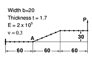
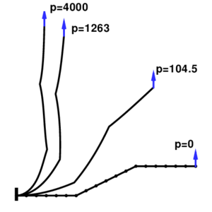
| − | This third example was extracted from a set of benchmarks for geometric non-linear behavior of structures <span id='citeF-19'></span>[[#cite-19|[19]]]. This benchmark is intended to assess membrane and bending actions, tension stiffening and change in sign of bending moments under large rotations and large displacements. Figure [[#img-10|10]].a shows the cross section properties, the material parameters and the initial geometry of a Z-shaped cantilever under a conservative load at the free end. Figure [[#img-10|10]].b shows the deformed configurations for three different values of the point load. These load values are defined as target values in Ref. <span id='citeF-19'></span>[[#cite-19|[19]]] to assess the element formulation. | + | This third example was extracted from a set of benchmarks for geometric non-linear behavior of structures <span id='citeF-19'></span>[[#cite-19|[19]]]. This benchmark is intended to assess membrane and bending actions, tension stiffening and change in sign of bending moments under large rotations and large displacements. Figure [[#img-10|10]].a shows the cross section properties, the material parameters and the initial geometry of a Z-shaped cantilever under a conservative load at the free end. Figure [[#img-10|10]].b shows the deformed configurations for three different values of the point load. These load values are defined as target values in Ref. <span id='citeF-19'></span>[[#cite-19|[19]]] to assess the element formulation. |
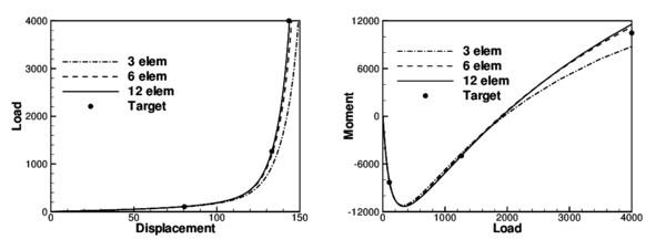
In Figure [[#img-10|10]].c and d the results for meshes with 3, 6 and 12 elements per zone are shown along all the process. In Figure [[#img-10|10]].c the load versus the tip displacement has been plotted while the bending moment at A versus the load is shown in Figure [[#img-10|10]].d. The bending moment plotted is obtained as the average of the bending moments computed at the integration points adjacent to point A. The results obtained with the B2 element show a very good agreement with the three expected values for the mesh with 6 elements per zone. | In Figure [[#img-10|10]].c and d the results for meshes with 3, 6 and 12 elements per zone are shown along all the process. In Figure [[#img-10|10]].c the load versus the tip displacement has been plotted while the bending moment at A versus the load is shown in Figure [[#img-10|10]].d. The bending moment plotted is obtained as the average of the bending moments computed at the integration points adjacent to point A. The results obtained with the B2 element show a very good agreement with the three expected values for the mesh with 6 elements per zone. | ||
| − | To assess convergence as the mesh is refined in the non-linear range Figures [[#img-10|10]].e and f plots for <math display="inline">P=104.5</math> and <math display="inline">P=1263</math> the normalized tip displacement and normalized moment at point A as a function of the number of DOFs in the mesh. The target values from Ref <span id='citeF-19'></span>[[#cite-19|[19]]] where used for normalization. It can be seen that the element has good convergence properties for both displacements and moments, while the element B21 of program ABAQUS <span id='citeF-20'></span>[[#cite-20|[20]]] shows excellent convergence properties for the displacement but a very slow convergence for the moments. | + | <div id='img-10'></div> |
| + | {| class="floating_imageSCP" style="text-align: center; border: 1px solid #BBB; margin: 1em auto; width: 100%;max-width: 100%;" | ||
| + | |- | ||
| + | |[[Image:Draft_Samper_148409403-fig10a.png|300px|]] | ||
| + | |[[Image:Draft_Samper_148409403-fig10b.png|300px|]] | ||
| + | |- | ||
| + | |colspan="2"|[[Image:Draft_Samper_148409403-fig10cd.png|600px|]] | ||
| + | |- | ||
| + | |[[Image:Draft_Samper_148409403-fig10e.png|300px|]] | ||
| + | |[[Image:Draft_Samper_148409403-fig10f.png|300px|]] | ||
| + | |- style="text-align: center; font-size: 75%;" | ||
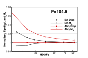
| + | | colspan="2" | '''Figure 10:''' Z-shaped cantilever. (a) Geometry and material; (b) Normalized displacements and moments as the mesh is refined; (c) Load versus tip displacement; (d) Bending moment at A versus load (e) and (f) convergence of the results in the non-linear range as the mesh is refined for P = 104.5 and <math>P = 1263</math> respectively. | ||
| + | |} | ||
| + | |||
| + | |||
| + | To assess convergence as the mesh is refined in the non-linear range Figures [[#img-10|10]].e and f plots for <math display="inline">P=104.5</math> and <math display="inline">P=1263</math> the normalized tip displacement and normalized moment at point A as a function of the number of DOFs in the mesh. The target values from Ref. <span id='citeF-19'></span>[[#cite-19|[19]]] where used for normalization. It can be seen that the element has good convergence properties for both displacements and moments, while the element B21 of program ABAQUS <span id='citeF-20'></span>[[#cite-20|[20]]] shows excellent convergence properties for the displacement but a very slow convergence for the moments. | ||
===6.3 Examples including large elastic-plastic strains=== | ===6.3 Examples including large elastic-plastic strains=== | ||
| Line 1,247: | Line 1,344: | ||
====6.3.1 Stretching of a circular sheet with an hemispherical punch==== | ====6.3.1 Stretching of a circular sheet with an hemispherical punch==== | ||
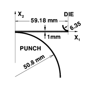
| − | First a well studied benchmark is considered<span id='citeF-22'></span>[[#cite-22|[22]]]. Figure [[#img-11|11]].a shows the initial configuration of the stretching of circular plate with an hemispherical punch. The material of the blank is a mild steel with <math display="inline">E = 6.9 \times{10}^{10}</math>, <math display="inline">\nu = 0.3</math> and tensile strength <math display="inline">\sigma _{y} = 5.89 \times{10}^{8} (0.0001+e^{p})^{0.216}</math>. | + | First a well studied benchmark is considered <span id='citeF-22'></span>[[#cite-22|[22]]]. Figure [[#img-11|11]].a shows the initial configuration of the stretching of circular plate with an hemispherical punch. The material of the blank is a mild steel with <math display="inline">E = 6.9 \times{10}^{10}</math>, <math display="inline">\nu = 0.3</math> and tensile strength <math display="inline">\sigma _{y} = 5.89 \times{10}^{8} (0.0001+e^{p})^{0.216}</math>. |
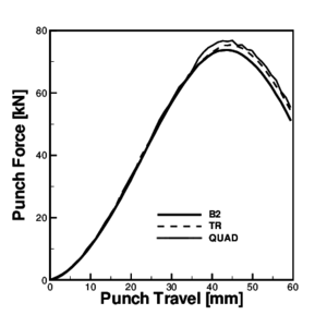
| − | The tools are assumed to be rigid and a frictionless interface was used. Contact between the tools and the sheet was considered via a penalty formulation. Two different meshes of 28 and 56 elements where used in the simulations with no practical differences in the results. Punch force versus punch travel is plotted in Figure [[#img-11|11]].b. Results obtained with the B2 element have been compared with those obtained using two solid element: a non-conforming triangle<span id='citeF-23'></span>[[#cite-23|[23]]] (TR) and a standard quadrilateral with constant pressure<span id='citeF-24'></span>[[#cite-24|[24]]] (QUAD). The results show a excellent agreement. | + | The tools are assumed to be rigid and a frictionless interface was used. Contact between the tools and the sheet was considered via a penalty formulation. Two different meshes of 28 and 56 elements where used in the simulations with no practical differences in the results. Punch force versus punch travel is plotted in Figure [[#img-11|11]].b. Results obtained with the B2 element have been compared with those obtained using two solid element: a non-conforming triangle <span id='citeF-23'></span>[[#cite-23|[23]]] (TR) and a standard quadrilateral with constant pressure <span id='citeF-24'></span>[[#cite-24|[24]]] (QUAD). The results show a excellent agreement. |
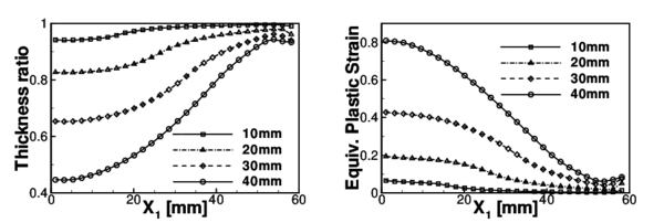
Figures [[#img-11|11]].c and [[#img-11|11]].d show the profiles of thickness ratio and equivalent plastic strain along the original radius for different stages of the simulation. These values compare quite well with the results obtained with the solid elements (not plotted for clarity). | Figures [[#img-11|11]].c and [[#img-11|11]].d show the profiles of thickness ratio and equivalent plastic strain along the original radius for different stages of the simulation. These values compare quite well with the results obtained with the solid elements (not plotted for clarity). | ||
| + | |||
| + | |||
| + | <div id='img-11'></div> | ||
| + | {| class="floating_imageSCP" style="text-align: center; border: 1px solid #BBB; margin: 1em auto; width: 100%;max-width: 100%;" | ||
| + | |- | ||
| + | |[[Image:Draft_Samper_148409403-fig11a.png|300px|]] | ||
| + | |[[Image:Draft_Samper_148409403-fig11b.png|300px|]] | ||
| + | |- | ||
| + | | colspan="2"|[[Image:Draft_Samper_148409403-fig11cd.png|600px|Punch stretching simulation of a thin metal sheet. (a)geometry; (b)punch force versus punch travel; (c)thickness ratio profiles as a function of the radius for different punch travels. (d)effective plastic strain (thickness averaged) profiles as a function of the radius for different punch travels.]] | ||
| + | |- style="text-align: center; font-size: 75%;" | ||
| + | | colspan="2" | '''Figure 11:''' Punch stretching simulation of a thin metal sheet. (a)geometry; (b)punch force versus punch travel; (c)thickness ratio profiles as a function of the radius for different punch travels. (d)effective plastic strain (thickness averaged) profiles as a function of the radius for different punch travels. | ||
| + | |} | ||
| + | |||
====6.3.2 Deep drawing and springback of a flat strip==== | ====6.3.2 Deep drawing and springback of a flat strip==== | ||
| − | The last example is a benchmark of NUMISHEET'93 <span id='citeF-25'></span>[[#cite-25|[25]]]. The aim of this example is to assess the forming process (deep drawing) of a thin sheet and the effects of the elastic springback after the tools are removed. Figure [[#img-12|12]].a shows the setting of the experiment. The geometrical parameters to be computed and compared with experimental results are shown in Figure [[#img-12|12]].b. Namely the angles <math display="inline">\theta _{1}</math> and <math display="inline">\theta _{2}\,</math> and the radius of curvature <math display="inline">\rho </math> of the lateral wall, obtained through the circle defined by points A, B and C. Due to the friction with the tools the shell is assumed to work in plane strain conditions (direction '''e'''<math display="inline">_{3}</math>) during the forming process. This assumption is kept for the springback step although the restriction of the tools is removed. Two different materials have been used for the simulations: aluminum and a mild steel. A complete definition of these materials can be found in <span id='citeF-25'></span>[[#cite-25|[25]]]. The material is assumed elastic-plastic. An isotropic behavior is used for the elastic component and an orthotropic yield function | + | The last example is a benchmark of NUMISHEET'93 <span id='citeF-25'></span>[[#cite-25|[25]]]. The aim of this example is to assess the forming process (deep drawing) of a thin sheet and the effects of the elastic springback after the tools are removed. Figure [[#img-12|12]].a shows the setting of the experiment. The geometrical parameters to be computed and compared with experimental results are shown in Figure [[#img-12|12]].b. Namely the angles <math display="inline">\theta _{1}</math> and <math display="inline">\theta _{2}\,</math> and the radius of curvature <math display="inline">\rho </math> of the lateral wall, obtained through the circle defined by points A, B and C. Due to the friction with the tools the shell is assumed to work in plane strain conditions (direction '''e'''<math display="inline">_{3}</math>) during the forming process. This assumption is kept for the springback step although the restriction of the tools is removed. Two different materials have been used for the simulations: aluminum and a mild steel. A complete definition of these materials can be found in <span id='citeF-25'></span>[[#cite-25|[25]]]. The material is assumed elastic-plastic. An isotropic behavior is used for the elastic component and an orthotropic yield function <span id='citeF-26'></span>[[#cite-26|[26]]] with exponential isotropic hardening is considered for the plastic component. For the simulations a low blank holder force (<math display="inline">2.45</math> kN) has been used. |
The deformed shape in Figure [[#img-12|12]].b corresponds to the simulation with aluminum. Figures [[#img-12|12]].c and d (obtained for aluminum and mild steel, respectively) show the geometrical parameters defined above obtained by different experimental groups (each abscissa corresponds to a different group). The average of the experimental values and those obtained with the B2 element are also shown. The numerical simulation agrees reasonably well between the rather scattered experimental values. | The deformed shape in Figure [[#img-12|12]].b corresponds to the simulation with aluminum. Figures [[#img-12|12]].c and d (obtained for aluminum and mild steel, respectively) show the geometrical parameters defined above obtained by different experimental groups (each abscissa corresponds to a different group). The average of the experimental values and those obtained with the B2 element are also shown. The numerical simulation agrees reasonably well between the rather scattered experimental values. | ||
| + | |||
| + | |||
| + | <div id='img-12'></div> | ||
| + | {| class="floating_imageSCP" style="text-align: center; border: 1px solid #BBB; margin: 1em auto; width: 100%;max-width: 100%;" | ||
| + | |- | ||
| + | |[[Image:Draft_Samper_148409403-fig12a.png|330px|]] | ||
| + | |[[Image:Draft_Samper_148409403-fig12b.png|270px|]] | ||
| + | |- | ||
| + | | colspan="2"|[[Image:Draft_Samper_148409403-fig12cd.png|600px|2-D Draw bending. (a) Geometry. (b) Geometrical parameters to measure the springback. (c) Comparison with experimental values (aluminum); (d) Comparison with experimental values (mild steel).]] | ||
| + | |- style="text-align: center; font-size: 75%;" | ||
| + | | colspan="2" | '''Figure 12:''' 2-D Draw bending. (a) Geometry. (b) Geometrical parameters to measure the springback. (c) Comparison with experimental values (aluminum); (d) Comparison with experimental values (mild steel). | ||
| + | |} | ||
==7 Conclusions== | ==7 Conclusions== | ||
| Line 1,265: | Line 1,387: | ||
==Acknowledgments== | ==Acknowledgments== | ||
| − | The first author is a member of the scientific staff of the Science Research Council of Argentina (CONICET). The support provided by a grant of CONICET is gratefully acknowledged. Financial support from CIMNE and support from Quantech ATZ (Barcelona-Spain) for providing Stampack, are also acknowledged | + | The first author is a member of the scientific staff of the Science Research Council of Argentina (CONICET). The support provided by a grant of CONICET is gratefully acknowledged. Financial support from CIMNE and support from Quantech ATZ (Barcelona-Spain) for providing Stampack, are also acknowledged. |
| − | == | + | ==References== |
<div id="cite-1"></div> | <div id="cite-1"></div> | ||
| Line 1,347: | Line 1,469: | ||
'''[[#citeF-26|[26]]]''' R. Hill. “A Theory of the Yielding and Plastic Flow of Anisotropic Metals”. ''Proc. Royal Society London'', Vol. '''A193''', pp. 281, 1948. | '''[[#citeF-26|[26]]]''' R. Hill. “A Theory of the Yielding and Plastic Flow of Anisotropic Metals”. ''Proc. Royal Society London'', Vol. '''A193''', pp. 281, 1948. | ||
| − | ==APPENDIX== | + | ==APPENDIX A== |
The variation <math display="inline">\delta \phi ^{1}</math> can be obtained noting that | The variation <math display="inline">\delta \phi ^{1}</math> can be obtained noting that | ||
| Line 1,357: | Line 1,479: | ||
|- | |- | ||
| style="text-align: center;" | <math>\cos \phi ^{1} =\mathbf{t}\cdot \mathbf{t}_{l}=\mathbf{n}\cdot \mathbf{n}_{l}</math> | | style="text-align: center;" | <math>\cos \phi ^{1} =\mathbf{t}\cdot \mathbf{t}_{l}=\mathbf{n}\cdot \mathbf{n}_{l}</math> | ||
| − | | style="width: 5px;text-align: right;white-space: nowrap;" | ( | + | | style="width: 5px;text-align: right;white-space: nowrap;" | (84.a) |
|- | |- | ||
| style="text-align: center;" | <math> \sin \phi ^{1} =\mathbf{n}\cdot \mathbf{t}_{l}=-\mathbf{t}\cdot \mathbf{n}_{l}</math> | | style="text-align: center;" | <math> \sin \phi ^{1} =\mathbf{n}\cdot \mathbf{t}_{l}=-\mathbf{t}\cdot \mathbf{n}_{l}</math> | ||
| − | | style="width: 5px;text-align: right;white-space: nowrap;" | ( | + | | style="width: 5px;text-align: right;white-space: nowrap;" | (84.b) |
|} | |} | ||
|} | |} | ||
| − | Taking the variation of the Eq.([[#APPENDIX| | + | Taking the variation of the Eq.([[#APPENDIX|84]].a) |
<span id="eq-94"></span> | <span id="eq-94"></span> | ||
| Line 1,378: | Line 1,500: | ||
| style="text-align: center;" | <math> =-\sin \phi ^{1}\left( \frac{\delta \mathbf{\varphi }^{1}-\delta \mathbf{\varphi }^{2}}{L}\cdot \mathbf{n}+\frac{\delta \mathbf{\varphi }^{1}-\delta \mathbf{\varphi }^{l}}{L_{i}}\cdot \mathbf{n}_{l}\right) </math> | | style="text-align: center;" | <math> =-\sin \phi ^{1}\left( \frac{\delta \mathbf{\varphi }^{1}-\delta \mathbf{\varphi }^{2}}{L}\cdot \mathbf{n}+\frac{\delta \mathbf{\varphi }^{1}-\delta \mathbf{\varphi }^{l}}{L_{i}}\cdot \mathbf{n}_{l}\right) </math> | ||
|} | |} | ||
| − | | style="width: 5px;text-align: right;white-space: nowrap;" | ( | + | | style="width: 5px;text-align: right;white-space: nowrap;" | (85) |
|} | |} | ||
| − | In Eq.([[#eq-94| | + | In Eq.([[#eq-94|85]]) <math display="inline">\delta \mathbf{t}</math> has been obtained observing that '''t''' and '''n ''' are unit orthogonal vectors |
{| class="formulaSCP" style="width: 100%; text-align: left;" | {| class="formulaSCP" style="width: 100%; text-align: left;" | ||
| Line 1,390: | Line 1,512: | ||
| style="text-align: center;" | <math>\begin{array}{c}[c]{ccc}\mathbf{t}\cdot \mathbf{t}=1 & & \mathbf{t}\cdot \mathbf{n}=0\\ 2\mathbf{t}\cdot \delta \mathbf{t}=0 & & \delta \mathbf{t}\cdot \mathbf{n}+\mathbf{t}\cdot \delta \mathbf{n}=0 \end{array} </math> | | style="text-align: center;" | <math>\begin{array}{c}[c]{ccc}\mathbf{t}\cdot \mathbf{t}=1 & & \mathbf{t}\cdot \mathbf{n}=0\\ 2\mathbf{t}\cdot \delta \mathbf{t}=0 & & \delta \mathbf{t}\cdot \mathbf{n}+\mathbf{t}\cdot \delta \mathbf{n}=0 \end{array} </math> | ||
|} | |} | ||
| − | | style="width: 5px;text-align: right;white-space: nowrap;" | ( | + | | style="width: 5px;text-align: right;white-space: nowrap;" | (86) |
|} | |} | ||
| Line 1,402: | Line 1,524: | ||
| style="text-align: center;" | <math>\delta \mathbf{t}=\left( \mathbf{n}\cdot \frac{\delta \mathbf{\varphi }^{2}-\delta \mathbf{\varphi }^{1}}{L}\right) \mathbf{n}</math> | | style="text-align: center;" | <math>\delta \mathbf{t}=\left( \mathbf{n}\cdot \frac{\delta \mathbf{\varphi }^{2}-\delta \mathbf{\varphi }^{1}}{L}\right) \mathbf{n}</math> | ||
|} | |} | ||
| − | | style="width: 5px;text-align: right;white-space: nowrap;" | ( | + | | style="width: 5px;text-align: right;white-space: nowrap;" | (87) |
|} | |} | ||
| − | Finally, from Eq.([[#eq-94| | + | Finally, from Eq.([[#eq-94|85]]) |
{| class="formulaSCP" style="width: 100%; text-align: left;" | {| class="formulaSCP" style="width: 100%; text-align: left;" | ||
| Line 1,414: | Line 1,536: | ||
| style="text-align: center;" | <math>\delta \phi ^{1}=\frac{\delta \mathbf{\varphi }^{1}-\delta \mathbf{\varphi }^{2}}{L}\cdot \mathbf{n}+\frac{\delta \mathbf{\varphi }^{1}-\delta \mathbf{\varphi }^{l}}{L_{l}}\cdot \mathbf{n}_{l}</math> | | style="text-align: center;" | <math>\delta \phi ^{1}=\frac{\delta \mathbf{\varphi }^{1}-\delta \mathbf{\varphi }^{2}}{L}\cdot \mathbf{n}+\frac{\delta \mathbf{\varphi }^{1}-\delta \mathbf{\varphi }^{l}}{L_{l}}\cdot \mathbf{n}_{l}</math> | ||
|} | |} | ||
| − | | style="width: 5px;text-align: right;white-space: nowrap;" | ( | + | | style="width: 5px;text-align: right;white-space: nowrap;" | (88) |
|} | |} | ||
| Line 1,425: | Line 1,547: | ||
|- | |- | ||
| style="text-align: center;" | <math>\cos \phi ^{2} =\mathbf{t}\cdot \mathbf{t}_{r}</math> | | style="text-align: center;" | <math>\cos \phi ^{2} =\mathbf{t}\cdot \mathbf{t}_{r}</math> | ||
| − | | style="width: 5px;text-align: right;white-space: nowrap;" | ( | + | | style="width: 5px;text-align: right;white-space: nowrap;" | (89.a) |
|- | |- | ||
| style="text-align: center;" | <math> \sin \phi ^{2} =-\mathbf{n}\cdot \mathbf{t}_{r}</math> | | style="text-align: center;" | <math> \sin \phi ^{2} =-\mathbf{n}\cdot \mathbf{t}_{r}</math> | ||
| − | | style="width: 5px;text-align: right;white-space: nowrap;" | ( | + | | style="width: 5px;text-align: right;white-space: nowrap;" | (89.b) |
|} | |} | ||
| − | |||
| − | |||
| − | |||
| − | |||
| − | |||
| − | |||
| − | |||
| − | |||
| − | |||
| − | |||
| − | |||
| − | |||
| − | |||
| − | |||
| − | |||
| − | |||
| − | |||
| − | |||
| − | |||
| − | |||
| − | |||
| − | |||
| − | |||
| − | |||
| − | |||
| − | |||
| − | |||
| − | |||
| − | |||
| − | |||
| − | |||
| − | |||
| − | |||
| − | |||
| − | |||
| − | |||
| − | |||
| − | |||
| − | |||
| − | |||
| − | |||
| − | |||
| − | |||
| − | |||
| − | |||
| − | |||
| − | |||
| − | |||
| − | |||
| − | |||
| − | |||
| − | |||
| − | |||
| − | |||
| − | |||
| − | |||
| − | |||
| − | |||
| − | |||
| − | |||
| − | |||
| − | |||
| − | |||
| − | |||
| − | |||
| − | |||
| − | |||
| − | |||
| − | |||
| − | |||
| − | |||
| − | |||
| − | |||
| − | |||
| − | |||
| − | |||
| − | |||
| − | |||
| − | |||
| − | |||
| − | |||
| − | |||
| − | |||
| − | |||
| − | |||
| − | |||
| − | |||
| − | |||
| − | |||
| − | |||
| − | |||
| − | |||
| − | |||
| − | |||
| − | |||
| − | |||
| − | |||
| − | |||
| − | |||
| − | |||
| − | |||
| − | |||
| − | |||
| − | |||
| − | |||
| − | |||
| − | |||
| − | |||
| − | |||
| − | |||
| − | |||
| − | |||
| − | |||
| − | |||
| − | |||
|} | |} | ||
Latest revision as of 10:35, 19 October 2018
Published in Comput. Methods Appl. Mech. Engrg., Vol. 195, pp. 5297–5315, 2006
doi:10.1016/j.cma.2005.08.021
Abstract
In this paper a finite element for the non-linear analysis of two dimensional beams and axisymmetric shells is presented. The element uses classical thin shell assumptions (no transverse shear strains). The main feature of the element is that it has no rotational degrees of freedom. Curvatures are computed using geometrical information from the patch of three elements formed by the main element and the two neighbour (adjacent) elements. Special attention is devoted to non-smooth geometries and branching shells. An elastic-plastic material law is considered. Large strains are treated using a logarithmic strain measure and a through-the-thickness numerical integration of the constitutive equations. Several examples are presented including linear problems to study convergence properties, and non-linear problems for both elastic and elastic-plastic materials and large strains.
Keywords: finite elements, beams, axisymmetric shells, rotation-free element, large strains
1 Introduction
The development of numerical techniques for shell analysis without rotational degrees of freedom has been mainly associated to the finite differences method (see for example Refs. [1,2,3]. Nevertheless, the idea of developing finite elements without rotational DOFs is not new [4,5] and different attempts have been reported in the last twenty years [6,7,8,9,10]. Despite these attempts it is just in the last few years that reliable rotation-free elements for industrial applications have been developed [11,12,13,14]. All the approximations share in common the definition of a patch (neighborhood) of elements to interpolate the geometry and the displacements. The main difference between the different approaches is the interpolation of the geometry and the theoretical basis used. One of the main aspects that remains unsolved satisfactorily is the treatment of non-smooth surfaces and specially branching shells. An adequate handling of multiple surfaces, i.e. when more than two elements share a side or edge, is mandatory if the element is to be used for the analysis of aeronautic and naval structures or frame structures typical in buildings, among others.
In this paper two-dimensional shell problems are tackled (previous work in this line can be found in Ref. [15,16]) with special focus on non-smooth shells and branching lines. This work may be seen as a first step towards the development of three dimensional rotation-free shell finite elements capable of handling kinked and branching shells.
The outline of the paper is as follows. First a summary of the most relevant equations governing the kinematic behavior of two dimensional Kirchhoff-Love shells is presented. In Section 3 a two-node rotation-free finite element for the analysis of straight but non-homogeneous (different thickness or materials) beam/axisymmetric shells is developed. In Section 4 the element is extended to deal with curved and non-smooth shells. The formulation is extended further to branching shells in Section 5. Several examples are presented in Section 6 showing convergence properties in linear and non-linear problems. At the end of this section two examples including elasto-plasticity with large strains are shown. In Section 7 some conclusions are drawn.
2 Governing equations of beams and thin two-dimensional shells
In this section a summary of the most relevant equations governing the kinematic behavior of thin shells is presented. More details can be found in the wide literature dedicated to the subject [1]. In order to introduce the problem, the kinematics of two dimensional beams are considered. These equations are latter extended to axisymmetric shells.
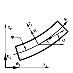
|
| Figure 1: Beam geometry and notation. |
2.1 Euler-Bernoulli beams
Within a classical Euler-Bernoulli beam theory (transverse shear strains disregarded) the geometry of a curved beam (see Figure 1) is completely defined by the position of central axis (line of centroids) as a function of the arc length measured from an arbitrary point on the reference (undeformed) configuration
|
|
(1) |
where are the Cartesian components referred to the canonical base . At each material point of the line of centroids associated to the coordinate it is possible to compute a convective system defined by the tangent to the line of centroids and the normal (in the plane)
|
|
(2) |
where is the normal to the beam plane.
The position of an arbitrary point located on the beam cross section can be written in terms of the position of the central line and the normal direction as a function of the distance of the point to the central axis as:
|
|
(3) |
The undeformed stress-free (natural) configuration will be used as the reference configuration where the material points are defined by their coordinates ( and ). Values measured on the reference configuration will be denoted with a left supra-index .
Dropping in the notation the dependence with the arc length , and denoting by , the in-plane deformation gradient is defined by
|
|
(4) |
While the right Cauchy-Green deformation tensor, restricted to the in-plane components is given by
|
|
(5) |
Disregarding terms associated with the only non trivial component of is
|
|
(6) |
We note that as the symmetric second order tensors considered are diagonal, only one index is used to alleviate notation when individual components are described.
The geometric measures of the central axis that allow to compute the strains are:
- The stretch of the line of centroids (squared)
|
|
(7) |
- The in-plane curvature of the line of centroids
|
|
(8) |
The later can also be expressed using the angle between the tangent and axis . Noting that
|
|
and that
|
|
then
|
|
(9) |
Above expressions (starting with (3)) assume a non-deformable cross section, which is adequate for negligible elastic small strains. For large or moderately large strains associated with an elastic-plastic behavior, it is necessary to modify the previous expressions to account for the section stretching. Here it will be assumed that the section does not modify its shape but its size, in such a way that the stretching of the line of centroids does not change the volume. Then, if the same stretching is supposed in both directions of the cross section and , the normal stretching is
|
|
(10) |
Note that this hypothesis does not imply any additional constraint on the beam theory neither an additional parameter. It is only introduced to update the distance of a point to the line of centroids (originally at a distant ) as . Consequently the present position of a point originally at will be written as:
|
|
(11) |
while the deformation gradient and the right Cauchy-Green deformation tensor are now
|
|
(12) |
|
|
(13) |
where the derivative of the normal stretching for the computation of the deformation gradient , and terms associated with in the definition of , have been disregarded.
2.2 Extension to axisymmetric shells
Assuming the axis of revolution coincident with axis , the extension of above expressions to axisymmetric shells requires the definition of the stretch in the circumferential direction (). This stretch depends only on the coordinate components over the axis in both present () and original () configurations. The additional non-trivial components of the deformation gradient and the deformation tensor are:
|
|
(14) |
|
|
(15) |
Disregarding the influence of distance in the denominator and consistently the influence of terms in in the numerator of Eq.(15) gives
|
For axisymmetric shells the stretching in the normal direction , using the isochoric assumption mentioned above, can be computed by
|
|
(18) |
The additional geometrical measures that allow to compute the strains are:
- The middle surface stretching in the circumferential direction directly related with the Green strain
|
|
(19) |
- The second principal (hoop) curvature
|
|
(20) |
In this way, the right Cauchy-Green deformation tensor can be written as (for the large strain case):
|
|
(21) |
2.3 Strain and stress measures
Note that for initially curved beams/shells, tensor (Eq. 21) is not the unit tensor, except for the points laying in the middle surface. Disregarding the influence of the initial curvatures in the definition of and defining the curvature changes as:
|
|
(22) |
it is possible to approximate (with the aim of an efficient numerical implementation) the expression of of Eq.(21) by
|
|
(23) |
The Green-Lagrange strain measures can be directly obtained from by:
|
where the strains at points out of the middle surface can be obtained by adding the strains at the middle surface and and the strains due to the curvatures.
To deal with moderately large or large strains, the most convenient strain measure is the logarithmic strain. Note that tensor is diagonal so that the principal strain directions are fixed (in material axis). Hence, the Hencky strain tensor components for an arbitrary point with coordinate along the normal are:
|
These strain measures can be associated with the (convective) Kirchhoff stress tensor through a constitutive equation adequate for large strains. The usual thin shell plane stress assumptions are used. In general, it is more convenient to write the weak form of the momentum equations in terms of the second Piola-Kirchhoff stress tensor related to the reference configuration. The relation between both stress tensors is:
|
The through-the-thickness integrated forces (generalized or resultant stresses) are:
|
|
(27) |
where is the original thickness of the beam/shell, is the original width ( for axisymmetric shells) and is the present distance (deformed) of the point to the middle line/surface. The weak form of the equilibrium conditions can be written as a virtual work equation. The internal virtual work (IVW) can be reduced to
|
|
(28) |
and
|
|
(29) |
for beams and axisymmetric shells, respectively.
3 Rotation-free beam/axisymmetric shell element
A two-node element with only translational degrees of freedom (rotation-free) is proposed. The geometrical configuration is defined by the positions of the two end nodes and (see Figure 2). For each element a linear interpolation for the line of centroids is proposed
|
|
(30) |
where are the standard linear Lagrangian polynomials (shape functions) defined over the interval . This allows the evaluation of middle surface stretches and the hoop curvature but it is not enough for the computation of the in-plane curvature . The later is computed resorting to the geometry of the surrounding elements leading to an assumed strain approach as shown below.
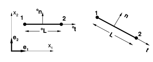
|
| Figure 2: Two-node element. |
3.1 Axial strain
The constant axial strain is easily computed from the element configuration. The tangent vector in the original configuration is:
|
|
(31) |
where , are the original position vectors of the element nodes and the initial element length given by
|
|
(32) |
Performing the same operations for the deformed configuration, we obtain
|
|
(33) |
|
|
(34) |
The axial stretch is
|
|
(35) |
and the Green-Lagrange strain of the line of centroids is computed as:
|
|
(36) |
while its variation is:
|
Matrix relating axial strain increment with nodal incremental displacements can be expressed as:
|
|
(38) |
where the incremental displacements at the nodes have been grouped in vector u.
3.2 Hoop strains in axisymmetric shells
The computation of the Green hoop strain at the middle surface (2.3.b) and the hoop change of curvature (22) associated to axisymmetric shells does not offer difficulties. Denoting with an upper index the node and with a lower index the component of the Cartesian system, in both the configuration and the displacement :
|
|
(39) |
|
|
(40) |
The variations of these strain measures, to be used in the weak form of the momentum equations, are:
|
|
|
(43) |
3.3 Evaluation of the in-plane curvature
For the in-plane curvature an assumed strain approach is adopted. The curvatures (9) are computed at the two nodes and a linear interpolation of these values is considered within the element
|
where a supra-index between brackets indicates the node of evaluation.
As in other rotation-free element, for the computation of the curvatures, the position of the nodes in the adjacent element is considered. In this case a patch of three elements (see Figure 3) is involved. There are different options for the computation of the curvatures at each element node. Initially an approximation adequate for smooth and homogeneous beam is defined. This approximation is latter modified to deal with more general geometries, including non-smooth and branching lines.
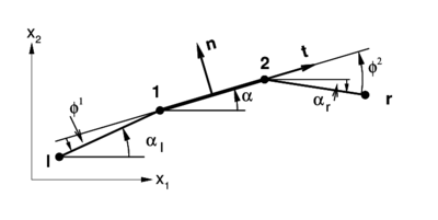
|
| Figure 3: Patch of elements used for the evaluation of the curvature. |
For the initial approximation of (9) the following (finite differences) computations can be used at each node:
a) the axial stretch at the node is computed as the average of the axial stretches at the adjacent elements
|
|
b) the derivative of the angle is computed as the difference of the angles between the tangent vectors divided by the average of the initial element lengths
|
|
then
|
In Eqs.(46) indexes and denote the left and right end nodes in the three elements patch (see Figure 3). Also and are the initial lengths of the elements respectively located at the right and the left of the central element in the patch.
For future reference the following angles must be identified
is, as defined above, the angle between the element (vector of Equation (33)) and the global axe
is the rotation of the element with respect to the original configuration (angle between vector and vector of Equation (31))
|
|
is the angle between two adjacent elements (relative angle). For example for the first node of the element (see Figure 3)
|
|
For the initially horizontal elements of Figure 3 the angle is also the rotation of the element. While the relative angle between the tangent vector of the central element () and the tangent vector of the left element () measured from to counter-clockwise (see Figure 4) is also the relative rotation . Similarly is the angle between the tangent vector of the central element () and the tangent vector of the right element () measured from to counter-clockwise.
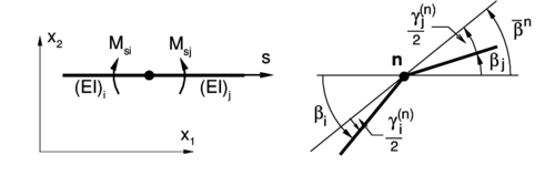
|
| Figure 4: Change of angle between elements. |
The approximation above leading to expressions (46) define a unique curvature value at each node, independently of the element from where it is computed. This represents a drawback for nonhomogeneous beams/shells, i.e. when there are changes in the material or in the transverse section properties of the beam/shell. Then at the intersection node of the two elements and of Figure 4 with different bending stiffness (), equilibrium can not be fulfilled at the node as
|
|
(47) |
because the nodal curvatures and are equal.
To avoid this problem, at each node shared by two elements ( and ), the nodal curvatures are re-defined independently for each element as:
|
|
(48) |
|
|
(49) |
(Note that lower indexes refer to element variables and upper indexes to nodal variables) where, with reference to Figure 4, is twice the difference between the rotation of the element and the rotation of the node (undefined yet)
|
The rotation of the node can be seen as the new position of a corrotational system from which curvatures are computed using the relative rotation . The sum of the relative rotations is of course the angle between both elements
|
|
(51) |
where the relative angle at node was defined above (see Figure 3).
Replacing the new definitions Eqs.(51) and (52) in the nodal equilibrium condition (50), for small strains (), it results:
|
Replacing Eq.(51) in the equilibrium relation (53) the values of can be expressed in terms of the relative angle and the stiffness measures ()
|
Finally, noting that the difference between the relative rotations is
|
|
(55) |
replacing Eq.(54) into (55) it allows to define the rotation of the node as:
|
|
(56) |
Then, the rotation of the node can be computed as the average of the rotation of the two adjacent elements weighted by their respective stiffness measure (). Above expressions (54) allow to compute the curvature at any point of the element by Eq.(45).
The variation of the curvature at an arbitrary point can be expressed as:
|
|
(57) |
From Eq. (49) the variation of the nodal curvature is composed of two parts
|
|
(58) |
The variations can be obtained as in (37c)
|
|
(59) |
While the variation can be obtained from (54) as (see Appendix):
|
Substituting Eqs. (59) and (60) into (58) gives
|
where gathers the displacements of all the nodes in the patch (although node have no contributions in the curvature at node ).
The variation of (48) is similarly obtained as:
|
Finally (57) can be written as:
|
Note that matrix is linear in the coordinate , then two integrations points are necessary to correctly integrate the tangent stiffness matrix or the residual force vector. If one integration point is desired some stabilization procedure is needed.
3.4 Boundary conditions
The imposition of translation boundary conditions associated with the line of centroids is straightforward as these are the element degrees of freedom. For boundary conditions affecting the rotation of the element normal, it must be noted that in such points the neighbor element does not exist. Two cases may be considered:
- Clamp or symmetry condition: in this case the rotation is null, i.e. the tangent to the beam/shell at that point is constant along the deformation, and equal to the normal to the symmetry (clamping) plane . The relative angle (in this case when the symmetric point is missing) can be expressed as twice the angle change between and the element tangent. If, for example, this restriction occurs in the first node of the element, the curvature at this node can be computed as:
|
|
also, noting that is constant, the curvature variation results:
|
|
- Free or simple supported edge: this is a natural boundary condition. The most straightforward approximation is to assume a null curvature at this point.
4 Curved and non-smooth beams/shells
In the above developments it is assumed a straight beam/shell, thus, the original angle between two elements is zero in the reference configuration. This is implicit in the way the in-plane curvatures where computed at each element node (3.3).
Consider now two elements that in the original configuration are not aligned. Assume that for the reference element the node under consideration is the first node. Using only the nodes position, it is not possible from the tangent vectors (or the normals ), to classify the node neighborhood as a curved line or a non-smooth line (a kink). This information must be explicitly supplied. Anyway, the handling of both cases is the same from practical purposes, because the effects due to the original curvatures are disregarded in the present formulation (see expression (23)).
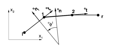
|
| Figure 5: Initial configuration for a non-smooth surface. |
Consider the configuration shown in Figure 5 where there exists an angle between the original tangents at each element defined by:
|
In the deformed configurations the tangent vectors and define a different angle ,
|
that represents a change with respect to the original configuration:
|
|
(71) |
The angle change so defined allows to compute the curvature changes at each of the two adjacent elements applying the same expressions derived in a previous section, i.e.: use Eqs. (54) to compute the relative rotation
|
and then use (48-49) to evaluate the curvature change at each element node
|
|
(73) |
5 More than two elements sharing a node (branching)
In a general case there can be elements sharing a node. The procedure for computing the in-plane curvature in terms of the nodal coordinates of the elements adjacents to the branching node is described below. Indeed the formulation of just two elements sharing a node described in the previous section is a particular case of the general approach here presented next.
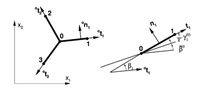
|
| Figure 6: Branching in beams. |
To alleviate the notation, it will be assumed that the intersection node (denoted by ) is the first node of each element, while the second node of each beam will also be defined (arbitrarily) as node (see Figure 6). In the original configuration, each element () configuration is completely defined by its tangent vector:
|
|
(74) |
As usual the element forms with the Cartesian axis an angle .
In the deformed configuration, the direction of element is computed as
|
|
(75) |
defining with the Cartesian axis an angle . The angle rotated by each element with respect to the original configuration is:
|
|
(76) |
Using the nodal equilibrium as above the rotation of the node is defined as the weighted average:
|
|
(77) |
Denoting again by twice the difference between the rotation of the node and the rotation of the element
|
|
(78) |
it is possible to write the in-plane change of curvature at the first node () of each element as:
|
|
(79) |
The variation of this in-plane curvature at the first node of each element gives:
|
|
(80) |
where for each element sharing the node
|
|
(81) |
and with this
|
|
(82) |
finally
|
|
(83) |
This allows to evaluate the variations of the in-plane curvature at the different elements sharing a branching node in order to compute the weak form of the momentum equations. It must be noted that the curvature variation depends on the nodal displacement variations of the nodes of all the elements sharing the branching node. Thus, the stiffness matrix of each element depends on all the nodes of the patch.
Note that above derivations hold both for beam and axisymmetric shell elements. The remaining of the strains in both elements are computed in the standard manner.
6 Numerical examples
In this section several examples are presented to assess the element described. This will be denoted as B2 (2-node Beam). Initially three linear examples are considered, then three geometrically non-linear (elastic) examples are shown, and finally a couple of examples including large strain plasticity (in smooth surfaces) are studied. All units are in the International System. The present element performance is compared with two transverse shear deformable two-node elements with 3 nodal degrees of freedom (two displacements and one rotation) and one integration point. Namely element B21 present in program ABAQUS [20], denoted here by Abq, and the element of Ref [17] denoted here by Sh, that should give identical results at least in the small strain elastic range. Note in the comparisons that using the shear deformable elements implies 50% more DOFs than when using element B2 for the same mesh.
6.1 Linear examples
The examples in the linear range are studied to assess the convergence properties of the B2 element. Comparisons with exact and converged numerical solutions are presented.
6.1.1 Simple supported beam under uniform load
The first example is a very simple one. A simple supported straight beam simply supported at both ends under a uniform transverse load in all its length. Due to symmetry only the left half of the beam is discretized. This allows to test both boundary conditions defined before for the normal rotation. Figure 7.a depicts the whole geometry.

|
| (a) |
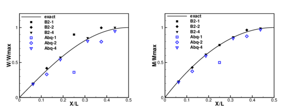
|
| Figure 7: Simple supported beam under uniform load. (a) geometry; (b) displacements; (c) bending moment. |
Different meshes have been considered to assess convergence, namely with 1, 2 and 4 elements. Nodes are uniformly distributed in the beam. In Figure 7.c the normalized displacement (respect to the exact maximum) has been plotted at the center of each element for the three meshes used, while Figure 7.d shows the normalized bending moment at the same points. Results obtained with element Abq are also shown for comparison.
It can be seen that when the mesh is refined convergence to the correct results is obtained. Four elements (8 for the whole beam) are enough to get accurate enough results. Convergence is faster for moments than for displacements, due probably to the fact that the element is non-conforming. For values computed at the element centers better results are obtained with element B2 than with the shear deformable elements using the same meshes.
6.1.2 Simple rigid-joined frame
The second examples considered is a two-beam frame with a sharp change of angle between two adjacent elements (see Figure 8.a). The horizontal member has a larger moment of inertia than the vertical member. An horizontal point load is applied as shown in the figure.
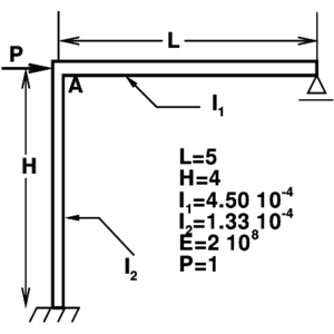
|
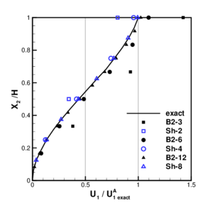
|
| (a) | (b) |
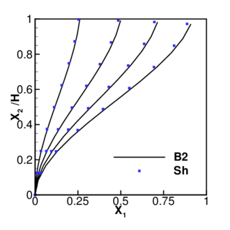
| |
| (c) | |
| Figure 8: Simple frame under point load. (a) geometry (b) horizontal displacements on the vertical member. (c) Deformed configurations in the non-linear range. | |
Figure 8.b shows the horizontal displacement over the vertical beam for the different meshes considered of 3, 6, and 12 elements discretizing each member. Results are normalized with respect to the exact displacement at joint A. Results obtained with the shear deformable element Sh with the same number of DOFs (2, 4 and 8 elements respectively) has also been plotted for reference. In this case it can be seen again that six elements at each member are needed to obtain accurate enough results from the engineering point of view, while four shear deformable elements would suffice for this case with a simple linear variation of the bending moment.
6.1.3 Branching axisymmetric shell
The third example considers a branching shell to assess the element formulation when more than two elements are joined at a node. Figure 9.a shows the geometry of the problem. The three parts of the shell have different thicknesses. The material is linear, elastic and isotropic with and . The spherical shell and the lower part of the cylinder are both subjected to internal pressure . This pressure is globally equilibrated by equal boundary forces at the ends of the cylinder.
Two meshes where considered in the discretization, one with 42 elements(18 for the lower cylinder, 16 for the sphere and 8 for the upper cylinder) and a second mesh with half the number of elements. The normal displacement along the cylinder has been plotted in Figure 9.b. Results obtained with the shear deformable element using the mesh of 42 elements and a converged finite element solution [18] are included for comparison (an analytical solution is also possible). For the finer mesh considered the results presented show an excellent agreement.

|
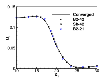
|
| (a) | (b) |
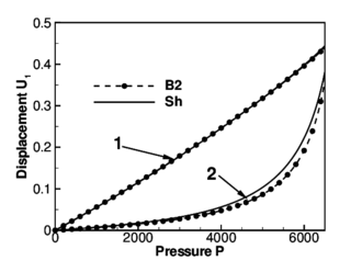
| |
| (c) | |
| Figure 9: Krauss' branching shell, (a) geometry , , , , , and (b) normal displacement along the cylinder. (c) Normal displacements at points 1 and 2 versus the internal pressure. | |
6.2 Examples including geometric non-linearity
In this section examples including large displacements and rotations are considered. Results obtained with present element are compared with results obtained with the shear deformable element. Two examples from the previous section, including sharp angles and branching, are now studied in the non-linear range. Also a well studied benchmark for non-smooth shells is analyzed to assess the convergence properties in the non-linear range.
6.2.1 Simple rigid-joined frame
The first example in this section is the simple two-bar frame considered before. A rather fine mesh of 12 elements on each bar has been considered. Figure 8.c shows the displacement profiles of the vertical bar for different values of the load . For the mesh considered the results are quite similar with those obtained using the shear deformable element (mesh with 8 elements in each bar and the same number of DOFs).
6.2.2 Branching axisymmetric shell
The second non-linear example considered includes a branching. This allows to assess convergence when more than two elements share a node in the non-linear range. Figure 9.c plots the normal displacements of points denoted as “1” and “2” in Figure 9.a as the internal pressure is increased.
The same finer mesh considered in the linear case (42 elements) was used. Results are compared with those obtained with the shear deformable element for the same mesh. The normal displacement of node 1 (branching node) is almost linear with the pressure and both elements give indistinguishable results. The displacements of point 2 (upper end of the cylinder) show some differences probably due the larger flexibility of the shear deformable element in this part of the shell where the thickness is maximum.
6.2.3 Elastic large deflection response of a Z-shaped cantilever
This third example was extracted from a set of benchmarks for geometric non-linear behavior of structures [19]. This benchmark is intended to assess membrane and bending actions, tension stiffening and change in sign of bending moments under large rotations and large displacements. Figure 10.a shows the cross section properties, the material parameters and the initial geometry of a Z-shaped cantilever under a conservative load at the free end. Figure 10.b shows the deformed configurations for three different values of the point load. These load values are defined as target values in Ref. [19] to assess the element formulation.
In Figure 10.c and d the results for meshes with 3, 6 and 12 elements per zone are shown along all the process. In Figure 10.c the load versus the tip displacement has been plotted while the bending moment at A versus the load is shown in Figure 10.d. The bending moment plotted is obtained as the average of the bending moments computed at the integration points adjacent to point A. The results obtained with the B2 element show a very good agreement with the three expected values for the mesh with 6 elements per zone.
To assess convergence as the mesh is refined in the non-linear range Figures 10.e and f plots for and the normalized tip displacement and normalized moment at point A as a function of the number of DOFs in the mesh. The target values from Ref. [19] where used for normalization. It can be seen that the element has good convergence properties for both displacements and moments, while the element B21 of program ABAQUS [20] shows excellent convergence properties for the displacement but a very slow convergence for the moments.
6.3 Examples including large elastic-plastic strains
In this section a couple of examples including large elastic-plastic strains are studied. In contrast with previous examples, the initial geometry of both cases is smooth. These simulations are performed with the explicitly dynamic program STAMPACK [21], oriented to the simulation of sheet metal forming processes.
6.3.1 Stretching of a circular sheet with an hemispherical punch
First a well studied benchmark is considered [22]. Figure 11.a shows the initial configuration of the stretching of circular plate with an hemispherical punch. The material of the blank is a mild steel with , and tensile strength .
The tools are assumed to be rigid and a frictionless interface was used. Contact between the tools and the sheet was considered via a penalty formulation. Two different meshes of 28 and 56 elements where used in the simulations with no practical differences in the results. Punch force versus punch travel is plotted in Figure 11.b. Results obtained with the B2 element have been compared with those obtained using two solid element: a non-conforming triangle [23] (TR) and a standard quadrilateral with constant pressure [24] (QUAD). The results show a excellent agreement.
Figures 11.c and 11.d show the profiles of thickness ratio and equivalent plastic strain along the original radius for different stages of the simulation. These values compare quite well with the results obtained with the solid elements (not plotted for clarity).
6.3.2 Deep drawing and springback of a flat strip
The last example is a benchmark of NUMISHEET'93 [25]. The aim of this example is to assess the forming process (deep drawing) of a thin sheet and the effects of the elastic springback after the tools are removed. Figure 12.a shows the setting of the experiment. The geometrical parameters to be computed and compared with experimental results are shown in Figure 12.b. Namely the angles and and the radius of curvature of the lateral wall, obtained through the circle defined by points A, B and C. Due to the friction with the tools the shell is assumed to work in plane strain conditions (direction e) during the forming process. This assumption is kept for the springback step although the restriction of the tools is removed. Two different materials have been used for the simulations: aluminum and a mild steel. A complete definition of these materials can be found in [25]. The material is assumed elastic-plastic. An isotropic behavior is used for the elastic component and an orthotropic yield function [26] with exponential isotropic hardening is considered for the plastic component. For the simulations a low blank holder force ( kN) has been used.
The deformed shape in Figure 12.b corresponds to the simulation with aluminum. Figures 12.c and d (obtained for aluminum and mild steel, respectively) show the geometrical parameters defined above obtained by different experimental groups (each abscissa corresponds to a different group). The average of the experimental values and those obtained with the B2 element are also shown. The numerical simulation agrees reasonably well between the rather scattered experimental values.
7 Conclusions
A finite element for non-linear, large strain, analysis of axisymmetric shells, beams has been presented. Smooth, kinked and branching situations have been considered. The main characteristic of the element formulation is that it does not include rotational degrees of freedom (rotation-free element). The curvature is computed resorting to the positions of the neighbor elements. The element can be considered as an “assumed strain element”, with a linear interpolation of the curvature. The numerical examples show that the element converges to the correct solution in all cases, and that the formulation can handle non-smooth surfaces and branching situations. Two integration points are necessary. Compared with the standard two-node shear deformable element this is a slight disadvantage when an explicit code is used. The element has given excellent results in problems including plasticity with large strains, contact with friction, different boundary conditions and loads.
Acknowledgments
The first author is a member of the scientific staff of the Science Research Council of Argentina (CONICET). The support provided by a grant of CONICET is gratefully acknowledged. Financial support from CIMNE and support from Quantech ATZ (Barcelona-Spain) for providing Stampack, are also acknowledged.
References
[1] A.C. Ugural. Stresses in Plates and Shells, McGraw Hill, New York, 1981.
[2] D. Bushnell and B.O. Almroth, “Finite difference energy method for non linear shell analysis”, J. Computers and Structures, Vol. 1, 361, 1971.
[3] D. Bushnell, “Computerized analysis of shells–-governing equations”, J. Computers and Structures, Vol. 18(3), 471-536, 1984.
[4] R.A. Nay and S. Utku. “An alternative to the finite element method”. Variational Methods Eng., Vol. 1, 1972.
[5] M.R. Barnes. Form finding and analysis of tension space structures by dynamic relaxation. Ph.D. Tesis, Department of Civil Engineering, The City University, London, 1977.
[6] J.K. Hampshire, B.H.V. Topping and H.C. Chan. “Three node triangular elements with one degree of freedom per node”. Engng. Comput. Vol. 9, pp. 49–62, 1992.
[7] R. Phaal and C.R. Calladine. “A simple class of finite elements for plate and shell problems. II: An element for thin shells with only translational degrees of freedom”. Int. J. Num. Meth. Engng., Vol. 5, pp. 979–996, 1992.
[8] E. Oñate and M. Cervera. “Derivation of thin plate bending elements with one degree of freedom per node”. Engineering Computations, Vol. 10, pp 553–561, 1993.
[9] G. Rio, B. Tathi and H. Laurent. A new efficient finite element model of shell with only three degrees of freedom per node. Applications to industrial deep drawing test. in Recent Developments in Sheet Metal Forming Technology, Ed. M.J.M. Barata Marques, 18th IDDRG Biennial Congress, Lisbon, 1994.
[10] M. Brunet and F. Sabourin. Prediction of necking and wrinkles with a simplified shell element in sheet forming. Int. Conf. of Metal Forming Simulation in Industry, Vol. II, pp. 27–48, B. Kröplin (Ed.), 1994.
[11] F. Cirak and M. Ortiz. Fully -conforming subdivision elements for finite deformations thin-shell analysis. Int. J. Num. Meths in Engng, vol. 51, 813-833, 2001.
[12] F.G. Flores and E. Oñate. A basic thin shell triangle with only translational DOFs for large strain plasticity. Int. J. Num. Meths in Engng, 51, pp. 57-83, 2001.
[13] E. Oñate, P. Cendoya and J. Miquel. Non linear explicit dynamic analysis of shells using the BST rotation-free triangle. Engineering Computations, vol.9(6), 662–706, 2002.
[14] F.G. Flores and E. Oñate. Improvements in the membrane behaviors of the three node rotation-free BST shell triangle using an assumed strain approach. Computer Methods in Applied Mechanics and Engineering, Vol. 194, pp 907-932, 2005.
[15] R. Phaal and C.R. Calladine. A simple class of finite elements for plate and shell problems. I: Elements for beams and thin plates. Int. J. Num. Meth. Engng., Vol. 5, pp. 955–977, 1992.
[16] J. Jovicevic and E. Oñate. Analysis of beams and shells using a rotation-free finite element-finite volume formulation, Monograph 43, CIMNE, Barcelona, 1999.
[17] F.G. Flores. Two Dimensional Shell Element for Nonlinear Analysis. Applied Mechanics Reviews, Vol. 48(11 part.2), pp.30-35. 1995.
[18] F.G. Flores y L.A. Godoy. Finite Element Applications to the Internal Pressure Loadings on Spherical Shells and other Shells of Revolution, Finite Element Analysis of Thin Walled Structures (Editor John Bull), Barking (England), Cap.9 pp. 259-296, 1990.
[19] Prinja NK and Clegg RA , A review of benchmark problems for geometric non-linear behaviors of 3-D beams and shells, NAFEMS R0024, 1993.
[20] Hibbit, Karlson and Sorensen Inc., ABAQUS, version 5.2.1, Pawtucket, USA.
[21] STAMPACK. version 6.0.0 A General Finite Element System for Sheet Stamping and Forming Problems, Quantech ATZ, Barcelona, Spain, (www.quantech.es), 2004.
[22] J.K. Lee, R. Wagoner, and E. Nakamachi. A benchmark test for sheet metal forming analysis, Technical Report, Ohio State University, 1990.
[23] F.G. Flores. A two-dimensional linear assumed strain triangular element for finite deformations analysis. Journal of Applied Mechanics (submitted) 2005.
[24] C.G. García Garino. A Numerical Model for Large Strain Analysis of Elasto-plastic Solids, (in Spanish). Ph.D. Thesis, Universidad Politécnica de Cataluña, 1993.
[25] A. Makinouchi et al (Ed), Proceedings of NUMISHEET 93 conference, Isehari, Japan, 1993.
[26] R. Hill. “A Theory of the Yielding and Plastic Flow of Anisotropic Metals”. Proc. Royal Society London, Vol. A193, pp. 281, 1948.
APPENDIX A
The variation can be obtained noting that
|
Taking the variation of the Eq.(84.a)
|
|
(85) |
In Eq.(85) has been obtained observing that t and n are unit orthogonal vectors
|
|
(86) |
then has components only along the direction :
|
|
(87) |
Finally, from Eq.(85)
|
|
(88) |
Similarly for node 2 where the angle is defined from to in such a way that:
|
Document information
Published on 01/01/2006
DOI: 10.1016/j.cma.2005.08.021
Licence: CC BY-NC-SA license
Share this document
Keywords
claim authorship
Are you one of the authors of this document?
