| (33 intermediate revisions by one other user not shown) | |||
| Line 1: | Line 1: | ||
| − | |||
| − | + | ==Acknowledgements== | |
| − | + | ||
| − | =Acknowledgements= | + | |
I would like to thank to all the people that in one way or other have helped me to complete my PhD. | I would like to thank to all the people that in one way or other have helped me to complete my PhD. | ||
| − | First of all, I would like to express my gratitude to my supervisor Prof. Xavier Oliver for his | + | First of all, I would like to express my gratitude to my supervisor Prof. Xavier Oliver for his supportfi and availability from the beginning and for his inexhaustible energy devoted to achieving the results of this dissertation. Today, I can say that if I feel the profession of scientist as my own is undoubtedly because of him. |
I really appreciate the confidence and patience of my co-advisor Juan Carlos Cante. I would like to thank all the fruitful scientific and personal discussions. I admire his ability to understand. | I really appreciate the confidence and patience of my co-advisor Juan Carlos Cante. I would like to thank all the fruitful scientific and personal discussions. I admire his ability to understand. | ||
| Line 27: | Line 24: | ||
I would like to give an special thank to my father, for his small gestures that show an enormous love. To my mother and Luis and the way they raised me, stood by me, and opened me to the world. To my sisters, Claudia, Julia and Marta for being there on my side and for the emotional support you provided to me. | I would like to give an special thank to my father, for his small gestures that show an enormous love. To my mother and Luis and the way they raised me, stood by me, and opened me to the world. To my sisters, Claudia, Julia and Marta for being there on my side and for the emotional support you provided to me. | ||
| − | + | ||
=Abstract= | =Abstract= | ||
| Line 109: | Line 106: | ||
The work developed in this research gives rise to the following scientific publications: | The work developed in this research gives rise to the following scientific publications: | ||
| − | + | '''A Ferrer, J Oliver JC Cante, and JA Hernández'''. Two-scale topology optimization: an efficient integrated structural optimization and material design approach. Draft, 2016. | |
| − | + | '''SM Giusti, A Ferrer and J Oliver''. Topological sensitivity analysis in heterogeneous anisotropic elasticity problem. Theoretical and computational aspects. Computer Methods in Applied Mechanics and Engineering, 2016. [http://www.sciencedirect.com/science/article/pii/S0045782516303577 http://dx.doi.org/10.1016/j.cma.2016.08.004] | |
| − | + | '''A Ferrer, J Oliver JC Cante, and O Lloberas'''. Vademecum-based approach to multi-scale topological material design. Advanced Modeling and Simulation in Engineering Sciences, 2016. [http://link.springer.com/article/10.1186/s40323-016-0078-4 doi:10.1186/s40323-016-0078-4] | |
| − | + | Additionally, the work has been presented in the following conferences and workshops: | |
| − | + | '''JC Cante, A Ferrer, J Oliver'''. Numerical tools for Multi-scale material design and structural topology optimization. In ECCOMAS VII European Congress on Computational Methods in Applied Sciences and Engineering, Creta, 2016. | |
| − | Vademecum-based approach | + | '''A Ferrer, J Oliver, JC Cante'''. Multi-scale topological design: a Vademecum-based approach. In New Challenges in Computational Mechanics (A Conference Celebration the 70th Birthday of Pierre Ladevèze), Paris, 2016. |
| − | + | '''J Oliver, JC Cante, A Ferrer'''. Computational design of engineering materials: An integrated multi-scale approach to structural topological optimization. In XIII International Conference on Computational Plasticity. Fundamentals and Applications. COMPLAS 2015, Barcelona 2015. | |
| − | + | '''A Ferrer, JC Cante, J Oliver'''. An efficient tool for multi-scale material design and structural topology optimization. In XIII International Conference on Computational Plasticity. Fundamentals and Applications. COMPLAS 2015, Barcelona, 2015. | |
| − | + | '''A Ferrer, JC Cante, J Oliver'''. On Multi-scale structural topology optimization and material design. In CMN-2016: Congress on numerical methods in Engineering, Lisbon, 2015. | |
| − | + | '''A Ferrer, JC Cante, J Oliver'''. Towards real time analysis in multi-scale computational design of engineering materials. In CSMA-SEMNI Numerical techniques for computation speedup, Biarritz, 2015. | |
| − | + | '''A Ferrer, J Oliver, A Huespe, JA Hernandez, JC Cante'''. On macrostructure and microstructure optimization techniques in multiscale computational material design. In 11th World Congress on Computational Mechanics, Barcelona 2014. | |
| − | + | '''A Huespe, J Oliver, A Ferrer, A Huespe, JA Hernandez, JC Cante'''. Hierarchical multiscale optimization of microstructure arrangement and macroscopic topology in computational material design. In XII International Conference on Computational Plasticity. Fundamentals and Applications. COMPLAS 2013, Barcelona, 2013. | |
| − | + | ||
| − | + | ||
| − | + | ||
| − | + | ||
| − | + | ||
| − | + | ||
| − | + | ||
| − | + | ||
| − | + | ||
| − | + | ||
| − | + | ||
| − | + | ||
| − | + | ||
| − | + | ||
| − | + | ||
| − | + | ||
| − | + | ||
| − | + | ||
| − | + | ||
| − | + | ||
| − | + | ||
| − | Hierarchical multiscale optimization of microstructure arrangement and macroscopic topology in computational material design. In XII International Conference on Computational Plasticity. Fundamentals and Applications. COMPLAS 2013, Barcelona, 2013. | + | |
Finally, the work of this dissemination has been complemented by the developments achieved in the following research stay: | Finally, the work of this dissemination has been complemented by the developments achieved in the following research stay: | ||
| − | + | '''Université dAvignon''', 4-month doctoral research stay. Worked under the supervision of Prof. Samuel Amstutz in the Laboratoire de Mathématiques dAvignon, Avignon, France. May-September 2016. | |
| − | |||
=2 Background and review of the state of the art= | =2 Background and review of the state of the art= | ||
| Line 538: | Line 512: | ||
Next step is to describe how the microscopic boundary conditions may be fulfilled. There are different approaches to satisfy these boundary conditions of the RVE. In literature, see <span id='citeF-4'></span>[[#cite-4|[4]]], the most frequently used can be classified in ''Taylor, Linear, Periodic'' and ''Minimal'' condition. | Next step is to describe how the microscopic boundary conditions may be fulfilled. There are different approaches to satisfy these boundary conditions of the RVE. In literature, see <span id='citeF-4'></span>[[#cite-4|[4]]], the most frequently used can be classified in ''Taylor, Linear, Periodic'' and ''Minimal'' condition. | ||
| − | + | '''Taylor boundary conditions'''. Frequently, this model is commonly termed, in other contexts, rule of mixtures <span id='citeF-5'></span>[[#cite-5|[5]]]. Intuitively, it homogenizes the properties by its volumetric contribution. In our terms, it turns into imposing zero fluctuation over all the domain (including the boundary), that is | |
| − | + | ||
| − | Frequently, this model is commonly termed, in other contexts, rule of mixtures <span id='citeF-5'></span>[[#cite-5|[5]]]. Intuitively, it homogenizes the properties by its volumetric contribution. In our terms, it turns into imposing zero fluctuation over all the domain (including the boundary), that is | + | |
<span id="eq-2.25"></span> | <span id="eq-2.25"></span> | ||
| Line 566: | Line 538: | ||
|} | |} | ||
| − | + | '''Linear boundary conditions'''. In comparison to the fluctuation on the ''Taylor conditions'', the linear boundary conditions are imposed to be zero only on the boundary, i.e, | |
| − | + | ||
| − | In comparison to the fluctuation on the ''Taylor conditions'', the linear boundary conditions are imposed to be zero only on the boundary, i.e, | + | |
<span id="eq-2.27"></span> | <span id="eq-2.27"></span> | ||
| Line 609: | Line 579: | ||
Since less conditions are imposed, ''Linear boundary conditions'' are less stiffer than the ''Taylor boundary conditions.'' However, there is still room to impose softer ones. | Since less conditions are imposed, ''Linear boundary conditions'' are less stiffer than the ''Taylor boundary conditions.'' However, there is still room to impose softer ones. | ||
| − | + | '''Periodic boundary conditions'''. Alternatively, the periodic boundary conditions are the ones with better reputation in the multi-scale field. In the literature, there are numerical studies that suggest its use in periodic material <span id='citeF-6'></span>[[#cite-6|[6]]]. The main advantage lies on the fact that, the size of the micro-structure in which the material is statistically representative, is the smaller size in comparison to the rest of boundary conditions. Thus, the condition on the jump of scales is easier to satisfy. | |
| − | + | ||
| − | Alternatively, the periodic boundary conditions are the ones with better reputation in the multi-scale field. In the literature, there are numerical studies that suggest its use in periodic material <span id='citeF-6'></span>[[#cite-6|[6]]]. The main advantage lies on the fact that, the size of the micro-structure in which the material is statistically representative, is the smaller size in comparison to the rest of boundary conditions. Thus, the condition on the jump of scales is easier to satisfy. | + | |
The periodic boundary conditions satisfy the fluctuation condition as follows. For some specific micro-scale geometries like square cells (hexagonal cells and others can be easily extended), the boundary is divided in <math display="inline">\Gamma _{1}^{+}</math>, <math display="inline">\Gamma _{1}^{-}</math>, <math display="inline">\Gamma _{2}^{+}</math> and <math display="inline">\Gamma _{2}^{-}</math> with outward unit normal such that | The periodic boundary conditions satisfy the fluctuation condition as follows. For some specific micro-scale geometries like square cells (hexagonal cells and others can be easily extended), the boundary is divided in <math display="inline">\Gamma _{1}^{+}</math>, <math display="inline">\Gamma _{1}^{-}</math>, <math display="inline">\Gamma _{2}^{+}</math> and <math display="inline">\Gamma _{2}^{-}</math> with outward unit normal such that | ||
| Line 668: | Line 636: | ||
More specifically, the fluctuation on the left part of the square cell <math display="inline">\Gamma _{2}^{+}</math> must be equal to the fluctuation on the right part <math display="inline">\Gamma _{2}^{-}</math> and, similarly, on the up and bottom part. Physically, this feature permits considering other micro-cell surrounding the RVE, and thus, the fluctuation will vary periodically along the micro-cell, hence its name. | More specifically, the fluctuation on the left part of the square cell <math display="inline">\Gamma _{2}^{+}</math> must be equal to the fluctuation on the right part <math display="inline">\Gamma _{2}^{-}</math> and, similarly, on the up and bottom part. Physically, this feature permits considering other micro-cell surrounding the RVE, and thus, the fluctuation will vary periodically along the micro-cell, hence its name. | ||
| − | + | '''Minimal boundary conditions'''. The minimum boundary conditions appear as the last alternative. They are considered the weaker boundary conditions since, in contrast to other boundary conditions, they assume no extra condition, hence its name. For this purpose, the fluctuation conditions ([[#eq-2.21|2.21]]) are imposed directly. | |
| − | + | ||
| − | The minimum boundary conditions appear as the last alternative. They are considered the weaker boundary conditions since, in contrast to other boundary conditions, they assume no extra condition, hence its name. For this purpose, the fluctuation conditions ([[#eq-2.21|2.21]]) are imposed directly. | + | |
Note that fluctuation condition ([[#eq-2.21|2.21]]) leads to impose that the integral over the boundary of the open product between the fluctuation and the outward unit normal is zero. That implies to impose six conditions in 3D problems and three conditions in 2D problems. | Note that fluctuation condition ([[#eq-2.21|2.21]]) leads to impose that the integral over the boundary of the open product between the fluctuation and the outward unit normal is zero. That implies to impose six conditions in 3D problems and three conditions in 2D problems. | ||
| − | + | '''Selected boundary condition and implementation strategy'''. The choice of the boundary condition is a priori arbitrary, and it would depend on the addressed problem. In our study, and throughout all this work, we select the periodic boundary conditions since they can ensure a representative volume with the smaller length scale <math display="inline">l_{\mu }</math>. | |
| − | + | ||
| − | The choice of the boundary condition is a priori arbitrary, and it would depend on the addressed problem. In our study, and throughout all this work, we select the periodic boundary conditions since they can ensure a representative volume with the smaller length scale <math display="inline">l_{\mu }</math>. | + | |
Regarding the way to impose the boundary conditions, there are two options. On the one hand, it can be imposed directly in the equilibrium problem and consequently the Lagrange multipliers appear as extra unknowns. On the other hand, it is possible to condensate some unknowns on the system through the boundary conditions. | Regarding the way to impose the boundary conditions, there are two options. On the one hand, it can be imposed directly in the equilibrium problem and consequently the Lagrange multipliers appear as extra unknowns. On the other hand, it is possible to condensate some unknowns on the system through the boundary conditions. | ||
| Line 682: | Line 646: | ||
The first option seems reasonable for small number of conditions like minimum conditions, however, for other kind of conditions, it enlarges the system of equations considerably. The option of condensing the unknowns in periodic and linear seems reasonable. As a difficulty, if iterative solvers are used, specially for large 3D problems, the condensation process confers worse conditioning to the matrix, lengthening the convergence process. If direct solvers are used, with the condensation technique, the matrix becomes less sparse bringing problems with memory. This features that the appropiate approach will depend on the specific problem to be solved. In our case, and through all this work, since not computationally high demanding meshes are required, the condensation process is considered. | The first option seems reasonable for small number of conditions like minimum conditions, however, for other kind of conditions, it enlarges the system of equations considerably. The option of condensing the unknowns in periodic and linear seems reasonable. As a difficulty, if iterative solvers are used, specially for large 3D problems, the condensation process confers worse conditioning to the matrix, lengthening the convergence process. If direct solvers are used, with the condensation technique, the matrix becomes less sparse bringing problems with memory. This features that the appropiate approach will depend on the specific problem to be solved. In our case, and through all this work, since not computationally high demanding meshes are required, the condensation process is considered. | ||
| − | + | '''Strong form of the microscopic equilibrium equation'''. Once the boundary conditions have been introduced, the strong form of the microscopic equilibrium equation can be stated. From the equilibrium equation in weak form ([[#eq-2.17|2.17]]), and undoing the steps of integration by parts (and assuming some regularity), the equilibrium equation requires divergence free of the microscopic stresses. This is, | |
| − | + | ||
| − | Once the boundary conditions have been introduced, the strong form of the microscopic equilibrium equation can be stated. From the equilibrium equation in weak form ([[#eq-2.17|2.17]]), and undoing the steps of integration by parts (and assuming some regularity), the equilibrium equation requires divergence free of the microscopic stresses. This is, | + | |
<span id="eq-2.34"></span> | <span id="eq-2.34"></span> | ||
| Line 833: | Line 795: | ||
{| style="text-align: left; margin:auto;width: 100%;" | {| style="text-align: left; margin:auto;width: 100%;" | ||
|- | |- | ||
| − | | style="text-align: center;" | <math>\chi =\begin{array}{ccc}1 & & x\in \Omega ^{+}\\ 0 & & x\in \Omega ^{-} \end{array}</math> | + | | style="text-align: center;" | <math>\chi =\begin{cases}\begin{array}{ccc}1 & & x\in \Omega ^{+}\\ 0 & & x\in \Omega ^{-} \end{array}\end{cases} </math> |
|} | |} | ||
| style="width: 5px;text-align: right;white-space: nowrap;" | (2.42) | | style="width: 5px;text-align: right;white-space: nowrap;" | (2.42) | ||
| Line 904: | Line 866: | ||
{| style="text-align: left; margin:auto;width: 100%;" | {| style="text-align: left; margin:auto;width: 100%;" | ||
|- | |- | ||
| − | | style="text-align: center;" | <math>\mathbb{C}\mbox{( }\chi \mbox{)}=\begin{array}{ccc}\mathbb{C\hbox{+}} & & \chi=1,\\ \mathbb{C}^{-} & & \chi=0, \end{array}</math> | + | | style="text-align: center;" | <math>\mathbb{C}\mbox{( }\chi \mbox{)}=\begin{cases}\begin{array}{ccc}\mathbb{C\hbox{+}} & & \chi=1,\\ \mathbb{C}^{-} & & \chi=0, \end{array}\end{cases} </math> |
|} | |} | ||
| style="width: 5px;text-align: right;white-space: nowrap;" | (2.47) | | style="width: 5px;text-align: right;white-space: nowrap;" | (2.47) | ||
| Line 1,235: | Line 1,197: | ||
{| style="text-align: left; margin:auto;width: 100%;" | {| style="text-align: left; margin:auto;width: 100%;" | ||
|- | |- | ||
| − | | style="text-align: center;" | <math>\chi _{B(\hat{x},\varepsilon )}(x)=1 x\in B(\hat{x},\epsilon ), | + | | style="text-align: center;" | <math>\chi _{B(\hat{x},\varepsilon )}(x)= \left\{ \begin{array}{ll}1 & x\in B(\hat{x},\epsilon ),\\ |
| − | + | 0 & x\notin B(\hat{x},\epsilon ),\end{array}\right. </math> | |
| − | + | ||
|} | |} | ||
| style="width: 5px;text-align: right;white-space: nowrap;" | (3.6) | | style="width: 5px;text-align: right;white-space: nowrap;" | (3.6) | ||
| Line 1,250: | Line 1,211: | ||
{| style="text-align: left; margin:auto;width: 100%;" | {| style="text-align: left; margin:auto;width: 100%;" | ||
|- | |- | ||
| − | | style="text-align: center;" | <math>s(x)=-1 x\in \Omega ^{+}, | + | | style="text-align: center;" | <math>s(x)= \left\{ \begin{array}{ll} -1 & x\in \Omega ^{+},\\ |
| − | + | 1 & x\notin \Omega \hbox{ - }.\end{array}\right. </math> | |
| − | + | ||
|} | |} | ||
| style="width: 5px;text-align: right;white-space: nowrap;" | (3.7) | | style="width: 5px;text-align: right;white-space: nowrap;" | (3.7) | ||
| Line 1,421: | Line 1,381: | ||
{| style="text-align: left; margin:auto;width: 100%;" | {| style="text-align: left; margin:auto;width: 100%;" | ||
|- | |- | ||
| − | | style="text-align: center;" | <math>x\in \Omega ^{+}:D_{T}\mathcal{J}(\hat{x})=\mathbb{P}\sigma (u)(\widehat{x})\cdot \nabla ^{s}u(\widehat{x})\geq{0},\qquad | + | | style="text-align: center;" | <math>x\in \Omega ^{+}:D_{T}\mathcal{J}(\hat{x})=\mathbb{P}\sigma (u)(\widehat{x})\cdot \nabla ^{s}u(\widehat{x})\geq{0},\qquad ({\bf Case~A}) </math> |
|} | |} | ||
| style="width: 5px;text-align: right;white-space: nowrap;" | (3.19) | | style="width: 5px;text-align: right;white-space: nowrap;" | (3.19) | ||
| Line 1,432: | Line 1,392: | ||
{| style="text-align: left; margin:auto;width: 100%;" | {| style="text-align: left; margin:auto;width: 100%;" | ||
|- | |- | ||
| − | | style="text-align: center;" | <math>x\in \Omega ^{-}:D_{T}\mathcal{J}(\hat{x})=\mathbb{P}\sigma (u)(\widehat{x})\cdot \nabla ^{s}u(\widehat{x})\leq{0.}\qquad | + | | style="text-align: center;" | <math>x\in \Omega ^{-}:D_{T}\mathcal{J}(\hat{x})=\mathbb{P}\sigma (u)(\widehat{x})\cdot \nabla ^{s}u(\widehat{x})\leq{0.}\qquad ({\bf Case~B}) </math> |
|} | |} | ||
| style="width: 5px;text-align: right;white-space: nowrap;" | (3.20) | | style="width: 5px;text-align: right;white-space: nowrap;" | (3.20) | ||
| Line 1,441: | Line 1,401: | ||
As a summary of the variables and properties described so far, in Table [[#table-1|1]], we show the initial and modified topology properties, the shape functional increments and the topological derivative for the Case A and B in a compact form. | As a summary of the variables and properties described so far, in Table [[#table-1|1]], we show the initial and modified topology properties, the shape functional increments and the topological derivative for the Case A and B in a compact form. | ||
| − | {| class="floating_tableSCP wikitable" style="text-align: center; margin: 1em auto;min-width:50%; | + | |
| − | + | <div class="center" style="font-size: 75%;">'''Table 1'''. Interpretation of the topological derivative interpretations</div> | |
| + | |||
| + | {| class="floating_tableSCP wikitable" style="text-align: center; margin: 1em auto;min-width:50%;font-size:85%;" | ||
|- | |- | ||
| colspan='1' style="border-right: 2px solid;border-left: 2px solid;border-right: 2px solid;" | | | colspan='1' style="border-right: 2px solid;border-left: 2px solid;border-right: 2px solid;" | | ||
| Line 1,544: | Line 1,506: | ||
{| style="text-align: left; margin:auto;width: 100%;" | {| style="text-align: left; margin:auto;width: 100%;" | ||
|- | |- | ||
| − | | style="text-align: center;" | <math>\chi =1-H(\psi )=\begin{array}{ccc}1 & & \psi{<0},\\ 0 & & \psi{>0.} \end{array}</math> | + | | style="text-align: center;" | <math>\chi =1-H(\psi )=\left\{\begin{array}{ccc}1 & & \psi{<0},\\ 0 & & \psi{>0.} \end{array}\right.</math> |
|} | |} | ||
| style="width: 5px;text-align: right;white-space: nowrap;" | (3.24) | | style="width: 5px;text-align: right;white-space: nowrap;" | (3.24) | ||
| Line 1,587: | Line 1,549: | ||
{| style="text-align: left; margin:auto;width: 100%;" | {| style="text-align: left; margin:auto;width: 100%;" | ||
|- | |- | ||
| − | | style="text-align: center;" | <math>\left\{\begin{array}{cc}\psi (\hat{x})\leq{0} & \hat{x}\in \Omega ^{+}\\ \psi (\hat{x})\geq{0} & \hat{x}\in \Omega ^{-} \end{array}\right.\quad \hbox{and}\left\{\begin{array}{cc}g(\hat{x})\leq{0} & \hat{x}\in \Omega ^{+}\\ g(\hat{x})\geq{0} & \hat{x}\in \Omega ^{-}. \end{array}\right. </math> | + | | style="text-align: center;" | <math>\left\{\begin{array}{cc}\psi (\hat{x})\leq{0} & \hat{x}\in \Omega ^{+}\\ \psi (\hat{x})\geq{0} & \hat{x}\in \Omega ^{-} \end{array}\right.\quad \hbox{and }\quad \left\{\begin{array}{cc}g(\hat{x})\leq{0} & \hat{x}\in \Omega ^{+}\\ g(\hat{x})\geq{0} & \hat{x}\in \Omega ^{-}. \end{array}\right. </math> |
|} | |} | ||
| style="width: 5px;text-align: right;white-space: nowrap;" | (3.27) | | style="width: 5px;text-align: right;white-space: nowrap;" | (3.27) | ||
| Line 1,782: | Line 1,744: | ||
where <math display="inline">g(x)</math> stands for the topological derivative of the cost function <math display="inline">\mathcal{J}(\chi (\psi )</math>). Note that, the topological derivative of the volume constraint is equal to <math display="inline">1</math> and has been consequently omitted. Hereafter, for simplicity, the extended topological derivative <math display="inline">\hat{g}(x)</math> is also called topological derivative. | where <math display="inline">g(x)</math> stands for the topological derivative of the cost function <math display="inline">\mathcal{J}(\chi (\psi )</math>). Note that, the topological derivative of the volume constraint is equal to <math display="inline">1</math> and has been consequently omitted. Hereafter, for simplicity, the extended topological derivative <math display="inline">\hat{g}(x)</math> is also called topological derivative. | ||
| − | + | '''Inequality constraints''' The augmented Lagrangian scheme can be extended to minimization problems with inequality constraints. The main idea consists in retrieving the minimization problem with equality constraints by adding an extra variable <math display="inline">z</math>, often termed slack variable, to the minimization problem with inequality constraints. In mathematical terms, it reads as | |
| − | + | ||
| − | The augmented Lagrangian scheme can be extended to minimization problems with inequality constraints. The main idea consists in retrieving the minimization problem with equality constraints by adding an extra variable <math display="inline">z</math>, often termed slack variable, to the minimization problem with inequality constraints. In mathematical terms, it reads as | + | |
<span id="eq-3.39"></span> | <span id="eq-3.39"></span> | ||
| Line 1,894: | Line 1,854: | ||
{| style="text-align: left; margin:auto;width: 100%;" | {| style="text-align: left; margin:auto;width: 100%;" | ||
|- | |- | ||
| − | | style="text-align: center;" | <math>(z^{*})^{2}=z_{1}^{2} c(\psi )>-\frac{\lambda }{\rho } | + | | style="text-align: center;" | <math>(z^{*})^{2}=\left\{ \begin{array}{ll}z_{1}^{2} & c(\psi )>-\frac{\lambda }{\rho }\\ |
| − | + | z_{2}^{2} & c(\psi )<-\frac{\lambda }{\rho }\end{array}\right.</math> | |
| − | + | ||
|} | |} | ||
| style="width: 5px;text-align: right;white-space: nowrap;" | (3.47) | | style="width: 5px;text-align: right;white-space: nowrap;" | (3.47) | ||
| Line 1,961: | Line 1,920: | ||
{| style="text-align: left; margin:auto;width: 100%;" | {| style="text-align: left; margin:auto;width: 100%;" | ||
|- | |- | ||
| − | | style="text-align: center;" | <math> | + | | style="text-align: center;" | <math> \frac{\partial r}{\partial \lambda }= |
| − | + | \left\{\begin{array}{ll}0 & c(\psi )>-\frac{\lambda }{\rho }\\ | |
| − | + | -\frac{1}{\rho } & c(\psi )<-\frac{\lambda }{\rho }\end{array}\right. \quad \hbox{and}\quad \frac{\partial r}{\partial \psi }=\left\{\begin{array}{ll} \frac{\partial c}{\partial \psi } & c(\psi )>-\frac{\lambda }{\rho },\\ | |
| − | + | 0 & c(\psi )<-\frac{\lambda }{\rho }\end{array}\right. . </math> | |
| − | + | ||
|} | |} | ||
| style="width: 5px;text-align: right;white-space: nowrap;" | (3.52) | | style="width: 5px;text-align: right;white-space: nowrap;" | (3.52) | ||
| Line 1,978: | Line 1,936: | ||
{| style="text-align: left; margin:auto;width: 100%;" | {| style="text-align: left; margin:auto;width: 100%;" | ||
|- | |- | ||
| − | | style="text-align: center;" | <math>\lambda{+\rho}r=\lambda{+\rho}r c(\psi )>-\frac{\lambda }{\rho } | + | | style="text-align: center;" | <math>\lambda{+\rho}r= \left\{\begin{array}{ll} \lambda{+\rho}r & c(\psi )>-\frac{\lambda }{\rho }\\ |
| − | + | 0 & c(\psi )<-\frac{\lambda }{\rho }\end{array}\right. </math> | |
| − | + | ||
|} | |} | ||
| style="width: 5px;text-align: right;white-space: nowrap;" | (3.53) | | style="width: 5px;text-align: right;white-space: nowrap;" | (3.53) | ||
| Line 1,993: | Line 1,950: | ||
{| style="text-align: left; margin:auto;width: 100%;" | {| style="text-align: left; margin:auto;width: 100%;" | ||
|- | |- | ||
| − | | style="text-align: center;" | <math>(\lambda{+\rho}r)\frac{\partial r}{\partial \lambda }=0\quad \hbox{and}\quad (\lambda{+\rho}r)\frac{\partial r}{\partial \psi }=(\lambda{+\rho}r)\frac{\partial c}{\partial \psi } c(\psi )>-\frac{\lambda }{\rho }, | + | | style="text-align: center;" | <math>(\lambda{+\rho}r)\frac{\partial r}{\partial \lambda }=0\quad \hbox{and}\quad (\lambda{+\rho}r)\frac{\partial r}{\partial \psi }=\left\{\begin{array}{ll} (\lambda{+\rho}r)\frac{\partial c}{\partial \psi } & c(\psi )>-\frac{\lambda }{\rho },\\ |
| − | + | 0 & c(\psi )<-\frac{\lambda }{\rho }.\end{array}\right. </math> | |
| − | + | ||
|} | |} | ||
| style="width: 5px;text-align: right;white-space: nowrap;" | (3.54) | | style="width: 5px;text-align: right;white-space: nowrap;" | (3.54) | ||
| Line 2,065: | Line 2,021: | ||
As an advantage, this scheme allows using the same implementation for both cases; equalities or inequalities; by means of exchanging the constraint <math display="inline">c(\psi _{n})</math> with the constraint <math display="inline">r(\psi _{n},\lambda _{n})</math>. For further information, the reader is referred to the reference book <span id='citeF-71'></span>[[#cite-71|[71]]] for a rigorous description and work <span id='citeF-72'></span>[[#cite-72|[72]]] for applying to topological optimization problem. | As an advantage, this scheme allows using the same implementation for both cases; equalities or inequalities; by means of exchanging the constraint <math display="inline">c(\psi _{n})</math> with the constraint <math display="inline">r(\psi _{n},\lambda _{n})</math>. For further information, the reader is referred to the reference book <span id='citeF-71'></span>[[#cite-71|[71]]] for a rigorous description and work <span id='citeF-72'></span>[[#cite-72|[72]]] for applying to topological optimization problem. | ||
| − | + | '''Penalty value and algorithm'''. It is worth mentioning that giving an adequate value to the penalty variable is not an easy task. In the reference book <span id='citeF-71'></span>[[#cite-71|[71]]], it is suggested increasing the penalty during the iterations (when the constraint is not tightened enough). Similarly, in work <span id='citeF-77'></span>[[#cite-77|[77]]], it is proposed to increase the penalty every five iterations. However, our experience shows us that the penalty cannot increase unlimitedly. A very small value of the penalty will make the problem converge very slowly but if, on the contrary, is very high the solution oscillates with the risk of non-convergence. So, as it was mentioned before, the appropiate value of this parameter will depend on the problem and on the sensibility of the cost when varying the constraint. The numerical experiments, further presented, suggest to normalize the cost function and take a small value of the penalty. | |
| − | + | ||
| − | It is worth mentioning that giving an adequate value to the penalty variable is not an easy task. In the reference book <span id='citeF-71'></span>[[#cite-71|[71]]], it is suggested increasing the penalty during the iterations (when the constraint is not tightened enough). Similarly, in work <span id='citeF-77'></span>[[#cite-77|[77]]], it is proposed to increase the penalty every five iterations. However, our experience shows us that the penalty cannot increase unlimitedly. A very small value of the penalty will make the problem converge very slowly but if, on the contrary, is very high the solution oscillates with the risk of non-convergence. So, as it was mentioned before, the appropiate value of this parameter will depend on the problem and on the sensibility of the cost when varying the constraint. The numerical experiments, further presented, suggest to normalize the cost function and take a small value of the penalty. | + | |
A detailed scheme of the Augmented Lagrangian Slerp algorithm is presented in Algorithm [[#algorithm-1|1]]. | A detailed scheme of the Augmented Lagrangian Slerp algorithm is presented in Algorithm [[#algorithm-1|1]]. | ||
| − | + | <span id='algorithm-1'></span> | |
| − | {| style="margin: 1em auto;border: 1px solid darkgray;" | + | {| style="margin: 1em auto;border: 1px solid darkgray;font-size:85%;" |
|- | |- | ||
| | | | ||
| − | : | + | : '''Init:''' choose initial values of <math display="inline">\psi _0</math>, <math display="inline">\theta _{min}</math>, tol, <math display="inline">\kappa _{min}</math>, <math display="inline">\lambda _0</math> and <math display="inline">\rho </math> |
| − | + | : Compute <math display="inline">\sigma _0</math> and <math display="inline">u_0</math> from ([[#eq-2.46|2.46]]). | |
| − | Compute <math display="inline"> | + | : Compute <math display="inline">r_0</math> from ([[#eq-3.56|3.56]]) with <math display="inline">c_0</math> from ([[#eq-3.10|3.10]]). |
| − | Compute <math display="inline"> | + | : Compute <math display="inline">\hat{g}_0</math> from ([[#eq-3.58|3.58]]) with <math display="inline">g</math> computed from ([[#eq-3.18|3.18]]). |
| − | + | : '''while''' <math>\theta _{n} \geq \theta _{min} \mathbf{or} r_n \geq tol</math> '''do''' | |
| − | + | :: Set <math display="inline">\kappa = 1</math>, <math display="inline">k=1</math>, <math display="inline">\mathcal{L}_k = \mathcal{L}_n</math>, <math display="inline">\theta _k = \theta _n</math>. | |
| − | : | + | :: '''while''' <math>\mathcal{L}_k \geq \mathcal{L}_n</math> (line search) '''do''' |
| − | : | + | ::: Update <math display="inline">\psi _k</math> from ([[#eq-3.33|3.33]]) with <math display="inline">\kappa </math>, <math display="inline">\theta _k</math> and <math display="inline">\hat{g}_n</math>, and update <math display="inline">\chi _k</math> from ([[#eq-3.24|3.24]]). |
| − | :: | + | ::: Compute <math display="inline">\sigma _k</math> and <math display="inline">u_k</math> from ([[#eq-2.46|2.46]]). |
| − | ::Compute <math display="inline">\ | + | ::: Compute <math display="inline">\mathcal{L}_k</math> from ([[#eq-3.50|3.50]]), with <math display="inline">\mathcal{J}_k</math> from ([[#eq-3.16|3.16]]) and set <math display="inline">\kappa = \kappa /2</math> and <math display="inline">k = k+1</math>. |
| − | :: | + | :: Set <math display="inline">\sigma _{n+1} = \sigma _k</math>, <math display="inline">u_{n+1} = u_k</math>, <math display="inline">\mathcal{L}_{n+1} = \mathcal{L}_k</math>, <math display="inline">\psi _{n+1}=\psi _k</math> |
| − | :: | + | :: Compute <math display="inline">\theta _{n+1}</math> from ([[#eq-3.34|3.34]]) |
| − | ::Compute <math display="inline"> | + | :: Compute <math display="inline">r_{n+1}</math> from ([[#eq-3.56|3.56]]) with <math display="inline">r_0</math> from ([[#eq-3.10|3.10]]). |
| − | :: | + | :: Update <math display="inline">\lambda _{n+1}</math> from ([[#eq-3.57|3.57]]). |
| − | :: | + | :: Compute <math display="inline">\hat{g}_{n+1}</math> from ([[#eq-3.58|3.58]]) with <math display="inline">g</math> computed from ([[#eq-3.18|3.18]]) and set <math display="inline">n = n+1</math>. |
| + | |} | ||
| − | + | <div class="center" style="font-size: 75%;">'''Algorithm. 1''' Augmented Lagrangian slerp algorithm. The Lagrange multiplier is updated in every topology iteration, i.e.,'' Usawa''-like scheme is used.</div> | |
| − | + | ||
| − | + | ||
| − | + | ||
| − | + | ||
| − | + | ||
| − | + | ||
==3.4 Treatment of the interface == | ==3.4 Treatment of the interface == | ||
| Line 2,121: | Line 2,070: | ||
We proceed to examine how to deal with the bi-material problem, from the continuous and discrete point of view, and how the different treatments of the interface affect the cost and the topological derivative. | We proceed to examine how to deal with the bi-material problem, from the continuous and discrete point of view, and how the different treatments of the interface affect the cost and the topological derivative. | ||
| − | + | '''Formulation''' | |
In the bi-material problem, the domain <math display="inline">\Omega </math> is first divided in two parts, one sub-domain with a strong material <math display="inline">\mathbb{C}^{+}</math> and the other sub-domain with a weak material <math display="inline">\mathbb{C}^{-}</math>. Then, the classical form of the elastic problem (without considering, for simplicity, the body forces) is written as | In the bi-material problem, the domain <math display="inline">\Omega </math> is first divided in two parts, one sub-domain with a strong material <math display="inline">\mathbb{C}^{+}</math> and the other sub-domain with a weak material <math display="inline">\mathbb{C}^{-}</math>. Then, the classical form of the elastic problem (without considering, for simplicity, the body forces) is written as | ||
| Line 2,172: | Line 2,121: | ||
{| style="text-align: left; margin:auto;width: 100%;" | {| style="text-align: left; margin:auto;width: 100%;" | ||
|- | |- | ||
| − | | style="text-align: center;" | <math>\mathbb{\mathbb{\tilde{C}}}=\mathbb{C}^{+} \hbox{ in }T_{k}^{+} | + | | style="text-align: center;" | <math>\mathbb{\mathbb{\tilde{C}}}=\left\{\begin{array}{lll}\mathbb{C}^{+} & \hbox{ in } & T_{k}^{+}\\ |
| − | + | \mathbb{C}^{-} & \hbox{ in } & T_{k}^{-}\\ | |
| − | + | \mathbb{C}^{\Gamma } & \hbox{ in } & T_{k}^{\Gamma }\end{array}\right. . </math> | |
| − | + | ||
| − | + | ||
|} | |} | ||
| style="width: 5px;text-align: right;white-space: nowrap;" | (3.62) | | style="width: 5px;text-align: right;white-space: nowrap;" | (3.62) | ||
| Line 2,221: | Line 2,168: | ||
{| style="text-align: left; margin:auto;width: 100%;" | {| style="text-align: left; margin:auto;width: 100%;" | ||
|- | |- | ||
| − | | style="text-align: center;" | <math>\tilde{\chi }_{io}=1-H(\psi (x_{g}))=\begin{array}{ccc}1 & & \psi (x_{g})<0\\ 0 & & \psi (x_{g})>0 \end{array}</math> | + | | style="text-align: center;" | <math>\tilde{\chi }_{io}=1-H(\psi (x_{g}))=\left\{\begin{array}{ccc}1 & & \psi (x_{g})<0\\ 0 & & \psi (x_{g})>0 \end{array}\right.</math> |
|} | |} | ||
| style="width: 5px;text-align: right;white-space: nowrap;" | (3.65) | | style="width: 5px;text-align: right;white-space: nowrap;" | (3.65) | ||
| Line 2,260: | Line 2,207: | ||
{| style="text-align: left; margin:auto;width: 100%;" | {| style="text-align: left; margin:auto;width: 100%;" | ||
|- | |- | ||
| − | | style="text-align: center;" | <math>\mathbb{C}_{io}^{\Gamma }=\begin{array}{ccc}\mathbb{C}^{+} & & \psi (x_{g})<0\\ \mathbb{C}^{-} & & \psi (x_{g})>0. \end{array}</math> | + | | style="text-align: center;" | <math>\mathbb{C}_{io}^{\Gamma }=\left\{\begin{array}{ccc}\mathbb{C}^{+} & & \psi (x_{g})<0\\ \mathbb{C}^{-} & & \psi (x_{g})>0. \end{array}\right.</math> |
|} | |} | ||
| style="width: 5px;text-align: right;white-space: nowrap;" | (3.68) | | style="width: 5px;text-align: right;white-space: nowrap;" | (3.68) | ||
| Line 2,429: | Line 2,376: | ||
{| class="floating_imageSCP" style="text-align: center; border: 1px solid #BBB; margin: 1em auto; width: 100%;max-width: 100%;" | {| class="floating_imageSCP" style="text-align: center; border: 1px solid #BBB; margin: 1em auto; width: 100%;max-width: 100%;" | ||
|- | |- | ||
| − | |[[Image:draft_Samper_118254298-Interface.png| | + | |[[Image:draft_Samper_118254298-Interface.png|300px|The volume Ω<sub>Γ</sub> of the interface triangular element Tₖ<sup>Γ</sup> is divided into the sub-domains Ω<sub>Γ</sub>⁺ and Ω<sub>Γ</sub>⁻ with material properties \mathbbC⁺ and \mathbbC⁻ respectively.]] |
|- style="text-align: center; font-size: 75%;" | |- style="text-align: center; font-size: 75%;" | ||
| colspan="1" | '''Figure 12:''' The volume <math>\Omega _{\Gamma }</math> of the interface triangular element <math>T_{k}^{\Gamma }</math> is divided into the sub-domains <math>\Omega _{\Gamma }^{+}</math> and <math>\Omega _{\Gamma }^{-}</math> with material properties <math>\mathbb{C}^{+}</math> and <math>\mathbb{C}^{-}</math> respectively. | | colspan="1" | '''Figure 12:''' The volume <math>\Omega _{\Gamma }</math> of the interface triangular element <math>T_{k}^{\Gamma }</math> is divided into the sub-domains <math>\Omega _{\Gamma }^{+}</math> and <math>\Omega _{\Gamma }^{-}</math> with material properties <math>\mathbb{C}^{+}</math> and <math>\mathbb{C}^{-}</math> respectively. | ||
| Line 2,475: | Line 2,422: | ||
Note that in the rest of elements <math display="inline">T_{k}^{+}</math> and <math display="inline">T_{k}^{-}</math>, the standard relation between stresses and strains are retrieved. | Note that in the rest of elements <math display="inline">T_{k}^{+}</math> and <math display="inline">T_{k}^{-}</math>, the standard relation between stresses and strains are retrieved. | ||
| − | + | '''Regularized characteristic function definition''' Then, we define the regularized characteristic function as the volume fraction of the strong material, i.e. | |
| − | + | ||
| − | Then, we define the regularized characteristic function as the volume fraction of the strong material, i.e. | + | |
<span id="eq-3.83"></span> | <span id="eq-3.83"></span> | ||
| Line 2,503: | Line 2,448: | ||
|} | |} | ||
| − | |||
| − | Following the description of the <math display="inline">\mathbb{P}_{1}</math>-projection, we again recognize, in the mixed formulation approach, the following four different cases for computing the regularized characteristic function: | + | '''Regularized characteristic function computation''' Following the description of the <math display="inline">\mathbb{P}_{1}</math>-projection, we again recognize, in the mixed formulation approach, the following four different cases for computing the regularized characteristic function: |
'''Case A:''' <math>0\geq \psi (x_{3})\geq \psi (x_{2})\geq \psi (x_{1}).</math> Same as the <math>\mathbb{P}_{1}</math> projection approach. This is | '''Case A:''' <math>0\geq \psi (x_{3})\geq \psi (x_{2})\geq \psi (x_{1}).</math> Same as the <math>\mathbb{P}_{1}</math> projection approach. This is | ||
| Line 2,527: | Line 2,471: | ||
{| class="floating_imageSCP" style="text-align: center; border: 1px solid #BBB; margin: 1em auto; width: 100%;max-width: 100%;" | {| class="floating_imageSCP" style="text-align: center; border: 1px solid #BBB; margin: 1em auto; width: 100%;max-width: 100%;" | ||
|- | |- | ||
| − | |[[Image:draft_Samper_118254298-TriangleCoordinates.png| | + | |[[Image:draft_Samper_118254298-TriangleCoordinates.png|400px|Representation of a material discontinuity when using a level-set ψ described by \mathbbP₁ Finite Element functions. The level-set ψ cuts the triangle in the nodes x₁₃ and x₂₃ in Case B and in the nodes x₃₁ and x₂₁ in Case C.]] |
|- style="text-align: center; font-size: 75%;" | |- style="text-align: center; font-size: 75%;" | ||
| colspan="1" | '''Figure 13:''' Representation of a material discontinuity when using a level-set <math>\psi </math> described by <math>\mathbb{P}_{1}</math> Finite Element functions. The level-set <math>\psi </math> cuts the triangle in the nodes <math>x_{13}</math> and <math>x_{23}</math> in Case B and in the nodes <math>x_{31}</math> and <math>x_{21}</math> in Case C. | | colspan="1" | '''Figure 13:''' Representation of a material discontinuity when using a level-set <math>\psi </math> described by <math>\mathbb{P}_{1}</math> Finite Element functions. The level-set <math>\psi </math> cuts the triangle in the nodes <math>x_{13}</math> and <math>x_{23}</math> in Case B and in the nodes <math>x_{31}</math> and <math>x_{21}</math> in Case C. | ||
| Line 2,708: | Line 2,652: | ||
In this case, the element <math>T_{k}^{\Gamma }</math> is not considered an interface element. | In this case, the element <math>T_{k}^{\Gamma }</math> is not considered an interface element. | ||
| − | + | '''Comparison with other approaches''' In comparison with other approaches (''In or Out'' or ''<math>\mathbb{P}_{1}</math>-projection'' approach), the characteristic function on the interface <math display="inline">\tilde{\chi }_{m}</math> in the mixed formulation approach evolves continuously when moving the level-set function. Thus, the characteristic function is now defined in | |
| − | + | ||
| − | In comparison with other approaches (''In or Out'' or ''<math>\mathbb{P}_{1}</math>-projection'' approach), the characteristic function on the interface <math display="inline">\tilde{\chi }_{m}</math> in the mixed formulation approach evolves continuously when moving the level-set function. Thus, the characteristic function is now defined in | + | |
{| class="formulaSCP" style="width: 100%; text-align: left;" | {| class="formulaSCP" style="width: 100%; text-align: left;" | ||
| Line 2,736: | Line 2,678: | ||
In Table [[#table-2|2]], we summarize and compare the treatment of the interface in terms of the characteristic function and constitutive tensor by the ''In or Out approach'', ''<math>\mathbb{P}_{1}</math>-projection approach'' and ''the Mixed formulation approach''. | In Table [[#table-2|2]], we summarize and compare the treatment of the interface in terms of the characteristic function and constitutive tensor by the ''In or Out approach'', ''<math>\mathbb{P}_{1}</math>-projection approach'' and ''the Mixed formulation approach''. | ||
| − | + | ||
| − | + | <div class="center" style="font-size: 75%;">'''Table 2'''. Summary of the different approaches used to treat with the interface elements. In the ''Mixed formulation approach'', in contrast to the others approaches, the fictitious constitutive tensor on the interface <math>\mathbb{C}^{\Gamma }</math> is allowed to evolve continuously when varying the level-set function.</div> | |
| + | |||
| + | {| class="floating_tableSCP wikitable" style="text-align: center; margin: 1em auto;min-width:50%;font-size:85%;" | ||
|- | |- | ||
| colspan='1' style="border-right: 2px solid;border-left: 2px solid;border-right: 2px solid;" | | | colspan='1' style="border-right: 2px solid;border-left: 2px solid;border-right: 2px solid;" | | ||
| Line 2,805: | Line 2,749: | ||
At this point, the following question arises: ''how does the Mixed formulation affects the optimization problem, and more specifically, the cost and the gradient?'' | At this point, the following question arises: ''how does the Mixed formulation affects the optimization problem, and more specifically, the cost and the gradient?'' | ||
| − | + | '''Implications of the mixed formulation on the cost function''' Regarding the cost function <math display="inline">\mathcal{J}</math>, we examine the implications of the mixed formulation when considering the compliance function. It can usually be written as the work produced by the external forces, i.e., | |
| − | + | ||
| − | Regarding the cost function <math display="inline">\mathcal{J}</math>, we examine the implications of the mixed formulation when considering the compliance function. It can usually be written as the work produced by the external forces, i.e., | + | |
{| class="formulaSCP" style="width: 100%; text-align: left;" | {| class="formulaSCP" style="width: 100%; text-align: left;" | ||
| Line 2,834: | Line 2,776: | ||
and <math display="inline">\tilde{\mathbb{C}}</math> represents the regularized constitutive tensor described in equation ([[#eq-3.62|3.62]]). Thus, the implications of the mixed formulation on the cost function rely completely on the behavior of the regularized constitutive tensor <math display="inline">\mathbb{C}^{\Gamma }</math> on the interface elements. | and <math display="inline">\tilde{\mathbb{C}}</math> represents the regularized constitutive tensor described in equation ([[#eq-3.62|3.62]]). Thus, the implications of the mixed formulation on the cost function rely completely on the behavior of the regularized constitutive tensor <math display="inline">\mathbb{C}^{\Gamma }</math> on the interface elements. | ||
| − | + | '''Implications of the mixed formulation on the topological derivative''' In order to study the implications of the mixed formulation on the topological derivative, we first examine the stresses <math display="inline">\sigma </math>. To simplify the notation, let's define the averaging operator <math display="inline">s</math> as | |
| − | + | ||
| − | In order to study the implications of the mixed formulation on the topological derivative, we first examine the stresses <math display="inline">\sigma </math>. To simplify the notation, let's define the averaging operator <math display="inline">s</math> as | + | |
{| class="formulaSCP" style="width: 100%; text-align: left;" | {| class="formulaSCP" style="width: 100%; text-align: left;" | ||
| Line 2,891: | Line 2,831: | ||
{| style="text-align: left; margin:auto;width: 100%;" | {| style="text-align: left; margin:auto;width: 100%;" | ||
|- | |- | ||
| − | | style="text-align: center;" | <math>\tilde{\sigma }=\sigma ^{+}=\mathbb{C}^{+}:\nabla ^{s}u \hbox{ in }T_{k}^{+} | + | | style="text-align: center;" | <math>\tilde{\sigma }=\left\{\begin{array}{lll}\sigma ^{+}=\mathbb{C}^{+}:\nabla ^{s}u & \hbox{ in } & T_{k}^{+}\\ |
| − | + | \sigma ^{-}=\mathbb{C}^{-}:\nabla ^{s}u &\hbox{ in } & T_{k}^{-}\\ | |
| − | + | \sigma ^{\Gamma }=\mathbb{C}^{\Gamma }:\nabla ^{s}u & \hbox{ in } & T_{k}^{\Gamma }\end{array}\right. </math> | |
| − | + | ||
| − | + | ||
|} | |} | ||
| style="width: 5px;text-align: right;white-space: nowrap;" | (3.109) | | style="width: 5px;text-align: right;white-space: nowrap;" | (3.109) | ||
| Line 2,920: | Line 2,858: | ||
{| style="text-align: left; margin:auto;width: 100%;" | {| style="text-align: left; margin:auto;width: 100%;" | ||
|- | |- | ||
| − | | style="text-align: center;" | <math>\tilde{\mathbb{P}}=\mathbb{P}^{+} \hbox{ in }T_{k}^{+}, | + | | style="text-align: center;" | <math>\tilde{\mathbb{P}}=\left\{\begin{array}{lll} \mathbb{P}^{+} &\hbox{ in } & T_{k}^{+},\\ |
| − | + | \mathbb{P}^{-} & \hbox{ in } & T_{k}^{-},\\ | |
| − | + | \mathbb{P}^{\Gamma }=s(\mathbb{P}^{+},\mathbb{P}^{-},\chi ) & \hbox{ in } &T_{k}^{\Gamma }. \end{array}\right.</math> | |
| − | + | ||
| − | + | ||
|} | |} | ||
| style="width: 5px;text-align: right;white-space: nowrap;" | (3.111) | | style="width: 5px;text-align: right;white-space: nowrap;" | (3.111) | ||
| Line 2,937: | Line 2,873: | ||
{| style="text-align: left; margin:auto;width: 100%;" | {| style="text-align: left; margin:auto;width: 100%;" | ||
|- | |- | ||
| − | | style="text-align: center;" | <math>\tilde{g}=g^{+}=\sigma ^{+}:\mathbb{P}^{+}:\nabla ^{s}u \hbox{ in }T_{k}^{+}, | + | | style="text-align: center;" | <math>\tilde{g}= \left\{\begin{array}{lll} g^{+}=\sigma ^{+}:\mathbb{P}^{+}:\nabla ^{s}u &\hbox{ in } & T_{k}^{+},\\ |
| − | + | g^{-}=\sigma ^{-}:\mathbb{P}^{-}:\nabla ^{s}u & \hbox{ in } & T_{k}^{-},\\ g^{\Gamma }=s(g^{+},g^{-},\tilde{\chi }) & \hbox{ in } & T_{k}^{\Gamma }.\end{array}\right. </math> | |
| − | + | ||
| − | + | ||
| − | + | ||
|} | |} | ||
| style="width: 5px;text-align: right;white-space: nowrap;" | (3.112) | | style="width: 5px;text-align: right;white-space: nowrap;" | (3.112) | ||
| Line 2,972: | Line 2,905: | ||
In Table [[#table-3|3]], we summarize the values that the main variables of the topology optimization problem take in the strong material elements, in the weak material elements and in the interface elements. | In Table [[#table-3|3]], we summarize the values that the main variables of the topology optimization problem take in the strong material elements, in the weak material elements and in the interface elements. | ||
| − | + | ||
| − | + | ||
| − | + | <div class="center" style="font-size: 75%;">'''Table 3'''. Summary of the practical treatment of the interface in topology optimization. The volume averaging operator <math>s(\cdot ,\cdot ,\tilde{\chi })</math>, with fraction volume on the element <math>\tilde{\chi }</math>, regularizes the corresponding discontinuous property on such element. The regularization of the constitutive tensor ''<math>\tilde{\mathbb{C}}</math>'' can be understood as an homogenization (with Taylor boundary conditions) of an RVE with fraction volume <math>\tilde{\chi }</math>, i.e. <math>\tilde{\mathbb{C}}=\mathbb{C}^{h}</math>.</div> | |
| + | |||
| + | {| class="floating_tableSCP wikitable" style="text-align: center; margin: 1em auto;min-width:50%;font-size:85%;" | ||
|- | |- | ||
| colspan='1' style="border-right: 2px solid;border-left: 2px solid;border-right: 2px solid;" | | | colspan='1' style="border-right: 2px solid;border-left: 2px solid;border-right: 2px solid;" | | ||
| Line 3,156: | Line 3,091: | ||
{| style="text-align: left; margin:auto;width: 100%;" | {| style="text-align: left; margin:auto;width: 100%;" | ||
|- | |- | ||
| − | | style="text-align: center;" | <math>g(\tilde{\chi }_{m})=g^{+}=\sigma _{\mu }^{+}:\mathbb{P}^{+}:\nabla ^{s}u_{\mu } \hbox{ in }T_{k}^{+}, | + | | style="text-align: center;" | <math>g(\tilde{\chi }_{m})= \left\{\begin{array}{lll} g^{+}=\sigma _{\mu }^{+}:\mathbb{P}^{+}:\nabla ^{s}u_{\mu } & \hbox{ in } & T_{k}^{+},\\ |
| − | + | g^{-}=\sigma _{\mu }^{-}:\mathbb{P}^{-}:\nabla ^{s}u_{\mu } & \hbox{ in } & T_{k}^{-},\\ | |
| − | + | g^{\Gamma }=s(g^{+},g^{-},\tilde{\chi }_{m}) & \hbox{ in } & T_{k}^{\Gamma }.\end{array}\right. </math> | |
| − | + | ||
| − | + | ||
|} | |} | ||
| style="width: 5px;text-align: right;white-space: nowrap;" | (3.118) | | style="width: 5px;text-align: right;white-space: nowrap;" | (3.118) | ||
| Line 3,356: | Line 3,289: | ||
|} | |} | ||
| − | |||
| − | |||
|- style="text-align: center; font-size: 75%;" | |- style="text-align: center; font-size: 75%;" | ||
| colspan="1" | '''Figure 21:''' Bridge topology optimization problem. Topology representation of the initial, intermediate and final iterations. Note the similarity between the optimal topology computationally designed and the topology proposed by the industry (shown in Figure [[#img-20|20]]). | | colspan="1" | '''Figure 21:''' Bridge topology optimization problem. Topology representation of the initial, intermediate and final iterations. Note the similarity between the optimal topology computationally designed and the topology proposed by the industry (shown in Figure [[#img-20|20]]). | ||
| Line 3,463: | Line 3,394: | ||
{| class="floating_imageSCP" style="text-align: center; border: 1px solid #BBB; margin: 1em auto; width: 100%;max-width: 100%;" | {| class="floating_imageSCP" style="text-align: center; border: 1px solid #BBB; margin: 1em auto; width: 100%;max-width: 100%;" | ||
|- | |- | ||
| − | |[[Image: | + | |[[Image:Draft_Samper_118254298_2192_Figure25.png|300px|Topological derivative concept.]] |
|- style="text-align: center; font-size: 75%;" | |- style="text-align: center; font-size: 75%;" | ||
| colspan="1" | '''Figure 25:''' Topological derivative concept. | | colspan="1" | '''Figure 25:''' Topological derivative concept. | ||
| Line 3,547: | Line 3,478: | ||
{| class="floating_imageSCP" style="text-align: center; border: 1px solid #BBB; margin: 1em auto; width: 100%;max-width: 100%;" | {| class="floating_imageSCP" style="text-align: center; border: 1px solid #BBB; margin: 1em auto; width: 100%;max-width: 100%;" | ||
|- | |- | ||
| − | |[[Image: | + | |[[Image:Draft_Samper_118254298_8095_Figure26.png|340px|Description of the problem.]] |
|- style="text-align: center; font-size: 75%;" | |- style="text-align: center; font-size: 75%;" | ||
| colspan="1" | '''Figure 26:''' Description of the problem. | | colspan="1" | '''Figure 26:''' Description of the problem. | ||
| Line 3,699: | Line 3,630: | ||
{| style="text-align: left; margin:auto;width: 100%;" | {| style="text-align: left; margin:auto;width: 100%;" | ||
|- | |- | ||
| − | | style="text-align: center;" | <math>\left\{\begin{array}{rlcl}\mathrm{div}\left(\sigma _{\epsilon }(w)\right)& =0 & \hbox{ in} & R^{2}\\ \sigma _{\epsilon }(w) & =\mathbb{C}_{\epsilon }(\widehat{x})\nabla ^{s}w\\ w & \rightarrow{0} & \hbox{ at} & \infty \\ \lbrack\ | + | | style="text-align: center;" | <math>\left\{\begin{array}{rlcl}\mathrm{div}\left(\sigma _{\epsilon }(w)\right)& =0 & \hbox{ in} & R^{2}\\ \sigma _{\epsilon }(w) & =\mathbb{C}_{\epsilon }(\widehat{x})\nabla ^{s}w\\ w & \rightarrow{0} & \hbox{ at} & \infty \\ \lbrack\lbrack w\rbrack\rbrack & =0 & \hbox{ on} & \partial B_{1}\\ \lbrack\lbrack\sigma _{\epsilon }(w)\rbrack\rbrack n & =-\mathbb{S}\sigma (u)(\widehat{x})n & \hbox{ on} & \partial B_{1} \end{array}\right., </math> |
|} | |} | ||
| style="width: 5px;text-align: right;white-space: nowrap;" | (4.19) | | style="width: 5px;text-align: right;white-space: nowrap;" | (4.19) | ||
| Line 3,712: | Line 3,643: | ||
{| style="text-align: left; margin:auto;width: 100%;" | {| style="text-align: left; margin:auto;width: 100%;" | ||
|- | |- | ||
| − | | style="text-align: center;" | <math>\left\{\begin{array}{rlcl}\mathrm{div}(\sigma _{\epsilon }(\widetilde{u}_{\epsilon })) & =\epsilon \mathrm{div}(\nabla \mathbb{C}_{\epsilon }(\zeta )(x-\widehat{x})\nabla ^{s}w) & \hbox{ in} & \Omega \\ \widetilde{u}_{\epsilon } & =-\epsilon w & \hbox{ on} & \Gamma _{D}\\ \sigma (\widetilde{u}_{\epsilon })n & =-\epsilon \sigma (w)n & \hbox{ on} & \Gamma _{N}\\ \lbrack\lbrack\widetilde{u}_{\epsilon }\rbrack\rbrack& =0 & \hbox{ on} & \partial B_{\epsilon }\\ \lbrack\lbrack\sigma _{\epsilon }(\widetilde{u}_{\epsilon })\rbrack\ | + | | style="text-align: center;" | <math>\left\{\begin{array}{rlcl}\mathrm{div}(\sigma _{\epsilon }(\widetilde{u}_{\epsilon })) & =\epsilon \mathrm{div}(\nabla \mathbb{C}_{\epsilon }(\zeta )(x-\widehat{x})\nabla ^{s}w) & \hbox{ in} & \Omega \\ \widetilde{u}_{\epsilon } & =-\epsilon w & \hbox{ on} & \Gamma _{D}\\ \sigma (\widetilde{u}_{\epsilon })n & =-\epsilon \sigma (w)n & \hbox{ on} & \Gamma _{N}\\ \lbrack\lbrack\widetilde{u}_{\epsilon }\rbrack\rbrack & =0 & \hbox{ on} & \partial B_{\epsilon }\\ \lbrack\lbrack\sigma _{\epsilon }(\widetilde{u}_{\epsilon })\rbrack\rbrack n & =-\epsilon \lbrack\lbrack\left(\nabla \mathbb{C}_{\epsilon }\left(\zeta \right)n\right)\left(\nabla ^{s}u(\widehat{x})+\nabla ^{s}w\right)\rbrack\rbrack n & \hbox{ on} & \partial B_{\epsilon } \end{array}\right., </math> |
|} | |} | ||
| style="width: 5px;text-align: right;white-space: nowrap;" | (4.20) | | style="width: 5px;text-align: right;white-space: nowrap;" | (4.20) | ||
| Line 3,828: | Line 3,759: | ||
{| style="text-align: left; margin:auto;width: 100%;" | {| style="text-align: left; margin:auto;width: 100%;" | ||
|- | |- | ||
| − | | style="text-align: center;" | <math>\left\{\begin{array}{rlcl}\mathrm{div}\left(\sigma _{\epsilon }(w)\right)& =0 & \hbox{ in} & R^{2}\\ \sigma _{\epsilon }(w) & =\mathbb{C}_{\epsilon }(\widehat{x})\nabla ^{s}w\\ w & \rightarrow{0} & \hbox{ at} & \infty \\ \lbrack\ | + | | style="text-align: center;" | <math>\left\{\begin{array}{rlcl}\mathrm{div}\left(\sigma _{\epsilon }(w)\right)& =0 & \hbox{ in} & R^{2}\\ \sigma _{\epsilon }(w) & =\mathbb{C}_{\epsilon }(\widehat{x})\nabla ^{s}w\\ w & \rightarrow{0} & \hbox{ at} & \infty \\ \lbrack\lbrack w\rbrack\rbrack & =0 & \hbox{ on} & \partial B_{1}\\ \lbrack\lbrack\sigma _{\epsilon }(w)\rbrack\rbrack n & =Sn & \hbox{ on} & \partial B_{1} \end{array}\right., </math> |
|} | |} | ||
| style="width: 5px;text-align: right;white-space: nowrap;" | (4.28) | | style="width: 5px;text-align: right;white-space: nowrap;" | (4.28) | ||
| Line 3,976: | Line 3,907: | ||
{| style="text-align: left; margin:auto;width: 100%;" | {| style="text-align: left; margin:auto;width: 100%;" | ||
|- | |- | ||
| − | | style="text-align: center;" | <math>\mathbb{P}=\begin{array}{ccc}\mathbb{P}^{+}= & \mathbb{P}(\alpha ,\beta ,\gamma _{0},1,1,1) & x\in \Omega ^{+}\\ \mathbb{P}^{-}= & \mathbb{P}(\alpha ,\beta ,\frac{1}{\gamma _{0}},1,1,1) & x\in \Omega ^{-}. \end{array}</math> | + | | style="text-align: center;" | <math>\mathbb{P}=\left\{\begin{array}{ccc}\mathbb{P}^{+}= & \mathbb{P}(\alpha ,\beta ,\gamma _{0},1,1,1) & x\in \Omega ^{+}\\ \mathbb{P}^{-}= & \mathbb{P}(\alpha ,\beta ,\frac{1}{\gamma _{0}},1,1,1) & x\in \Omega ^{-}. \end{array}\right.</math> |
|} | |} | ||
| style="width: 5px;text-align: right;white-space: nowrap;" | (4.38) | | style="width: 5px;text-align: right;white-space: nowrap;" | (4.38) | ||
| Line 3,993: | Line 3,924: | ||
{| style="text-align: left; margin:auto;width: 100%;" | {| style="text-align: left; margin:auto;width: 100%;" | ||
|- | |- | ||
| − | | style="text-align: center;" | <math>\left\{\begin{array}{rlcl}\mathrm{div}\left(\sigma _{\epsilon }(w)\right)& =0 & \hbox{ in} & R^{2}\\ \sigma _{\epsilon }(w) & =\mathbb{C}_{\epsilon }(\widehat{x})\nabla ^{s}w\\ w & \rightarrow{0} & \hbox{ at} & \infty \\ \lbrack\ | + | | style="text-align: center;" | <math>\left\{\begin{array}{rlcl}\mathrm{div}\left(\sigma _{\epsilon }(w)\right)& =0 & \hbox{ in} & R^{2}\\ \sigma _{\epsilon }(w) & =\mathbb{C}_{\epsilon }(\widehat{x})\nabla ^{s}w\\ w & \rightarrow{0} & \hbox{ at} & \infty \\ \lbrack\lbrack w\rbrack\rbrack & =0 & \hbox{ on} & \partial B_{1}\\ \lbrack\lbrack\sigma _{\epsilon }(w)\rbrack\rbrack n & =Sn & \hbox{ on} & \partial B_{1} \end{array}\right., </math> |
|} | |} | ||
| style="width: 5px;text-align: right;white-space: nowrap;" | (4.39) | | style="width: 5px;text-align: right;white-space: nowrap;" | (4.39) | ||
| Line 4,148: | Line 4,079: | ||
{| style="text-align: left; margin:auto;width: 100%;" | {| style="text-align: left; margin:auto;width: 100%;" | ||
|- | |- | ||
| − | | style="text-align: center;" | <math>\mathbb{P}=\begin{array}{ccc}\mathbb{P}^{+}= & \mathbb{\mathbb{P}}(\mathbb{C}^{+},\mathbb{C}^{-}) & x\in \Omega ^{+}\\ \mathbb{P}^{-}= & \mathbb{\mathbb{P}}(\mathbb{C}^{-},\mathbb{C}^{+}) & x\in \Omega ^{-}. \end{array}</math> | + | | style="text-align: center;" | <math>\mathbb{P}=\left\{\begin{array}{ccc}\mathbb{P}^{+}= & \mathbb{\mathbb{P}}(\mathbb{C}^{+},\mathbb{C}^{-}) & x\in \Omega ^{+}\\ \mathbb{P}^{-}= & \mathbb{\mathbb{P}}(\mathbb{C}^{-},\mathbb{C}^{+}) & x\in \Omega ^{-}. \end{array}\right.</math> |
|} | |} | ||
| style="width: 5px;text-align: right;white-space: nowrap;" | (4.50) | | style="width: 5px;text-align: right;white-space: nowrap;" | (4.50) | ||
| Line 4,159: | Line 4,090: | ||
<span id='theorem-lem:ueps-u'></span> 1: Let <math display="inline">u</math> and <math display="inline">u_{\epsilon }</math> be solutions to ([[#eq-4.5|4.5]]) and ([[#eq-4.10|4.10]]), respectively. Then, we have that the estimate <math display="inline">\| u_{\epsilon }-u\| _{H^{1}(\Omega ;R^{2})}=O(\epsilon )</math> holds true. | <span id='theorem-lem:ueps-u'></span> 1: Let <math display="inline">u</math> and <math display="inline">u_{\epsilon }</math> be solutions to ([[#eq-4.5|4.5]]) and ([[#eq-4.10|4.10]]), respectively. Then, we have that the estimate <math display="inline">\| u_{\epsilon }-u\| _{H^{1}(\Omega ;R^{2})}=O(\epsilon )</math> holds true. | ||
| − | Proof 1: We start by subtracting the variational problem ([[#eq-4.5|4.5]]) and ([[#eq-4.10|4.10]]) to obtain: | + | '''Proof 1''': We start by subtracting the variational problem ([[#eq-4.5|4.5]]) and ([[#eq-4.10|4.10]]) to obtain: |
{| class="formulaSCP" style="width: 100%; text-align: left;" | {| class="formulaSCP" style="width: 100%; text-align: left;" | ||
| Line 4,190: | Line 4,121: | ||
{| style="text-align: left; margin:auto;width: 100%;" | {| style="text-align: left; margin:auto;width: 100%;" | ||
|- | |- | ||
| − | | style="text-align: center;" | <math>\int _{\Omega }\sigma _{\epsilon }(u_{\epsilon }-u)\cdot \nabla ^{s}(u_{\epsilon }-u) \leq C_{1}\| \sigma (u)\| _{L^{2}(B_{\epsilon };R^{2})}\| \nabla ^{s}(u_{\epsilon }-u)\| _{L^{2}(B_{\epsilon };R^{2})} | + | | style="text-align: center;" | <math>\begin{array}{lll}\int _{\Omega }\sigma _{\epsilon }(u_{\epsilon }-u)\cdot \nabla ^{s}(u_{\epsilon }-u) & \leq & C_{1}\| \sigma (u)\| _{L^{2}(B_{\epsilon };R^{2})}\| \nabla ^{s}(u_{\epsilon }-u)\| _{L^{2}(B_{\epsilon };R^{2})}\\ |
| − | + | & \leq & C_{2}\epsilon \| \nabla ^{s}(u_{\epsilon }-u)\| _{L^{2}(B_{\epsilon };R^{2})}\\ | |
| − | + | & \leq & C_{3}\epsilon \| \nabla ^{s}(u_{\epsilon }-u)\| _{H^{1}(\Omega ;R^{2})}\\ | |
| − | + | & \leq & C_{4}\epsilon \| u_{\epsilon }-u\| _{H^{1}(\Omega ;R^{2})},\end{array} </math> | |
| − | + | ||
| − | + | ||
| − | + | ||
|} | |} | ||
| style="width: 5px;text-align: right;white-space: nowrap;" | (4.53) | | style="width: 5px;text-align: right;white-space: nowrap;" | (4.53) | ||
| Line 4,229: | Line 4,157: | ||
with the constant <math display="inline">C</math> independent of the small parameter <math display="inline">\epsilon </math>. | with the constant <math display="inline">C</math> independent of the small parameter <math display="inline">\epsilon </math>. | ||
| − | Proof 2: From the ansatz proposed in ([[#eq-4.18|4.18]]) for <math display="inline">u_{\epsilon }</math> and making use of the triangular inequality, we obtain: | + | '''Proof 2''': From the ansatz proposed in ([[#eq-4.18|4.18]]) for <math display="inline">u_{\epsilon }</math> and making use of the triangular inequality, we obtain: |
{| class="formulaSCP" style="width: 100%; text-align: left;" | {| class="formulaSCP" style="width: 100%; text-align: left;" | ||
| Line 4,236: | Line 4,164: | ||
{| style="text-align: left; margin:auto;width: 100%;" | {| style="text-align: left; margin:auto;width: 100%;" | ||
|- | |- | ||
| − | | style="text-align: center;" | <math>|\widetilde{u}_{\epsilon }|_{H^{1}(\Omega ;R^{2})} = | + | | style="text-align: center;" | <math> \begin{array}{lll} |\widetilde{u}_{\epsilon }|_{H^{1}(\Omega ;R^{2})} & = & |u_{\epsilon }-u-\epsilon w|_{H^{1}(\Omega ;R^{2})}\\ |
| − | + | & \leq & |u_{\epsilon }-u|_{H^{1}(\Omega ;R^{2})}+\epsilon |w|_{H^{1}(\Omega ;R^{2})}\\ | |
| − | + | & \leq & \| u_{\epsilon }-u\| _{H^{1}(\Omega ;R^{2})}+\epsilon |w|_{H^{1}(R^{2};R^{2})}\\ | |
| − | + | & \leq & C_{1}\epsilon \,,\end{array} </math> | |
| − | + | ||
| − | + | ||
| − | + | ||
|} | |} | ||
| style="width: 5px;text-align: right;white-space: nowrap;" | (4.56) | | style="width: 5px;text-align: right;white-space: nowrap;" | (4.56) | ||
| Line 4,249: | Line 4,174: | ||
where we have used the change of variables <math display="inline">x=\epsilon y</math>, the equivalence between the semi-norm and the norm in <math display="inline">H^{1}(\Omega ;R^{2})</math> and the estimate in Lemma [[#theorem-lem:ueps-u|1]]. Finally, the results comes out from the Poincaré inequality. | where we have used the change of variables <math display="inline">x=\epsilon y</math>, the equivalence between the semi-norm and the norm in <math display="inline">H^{1}(\Omega ;R^{2})</math> and the estimate in Lemma [[#theorem-lem:ueps-u|1]]. Finally, the results comes out from the Poincaré inequality. | ||
| − | + | 3: Let <math display="inline">\widetilde{u}_{\epsilon }</math> and <math display="inline">u</math> be solutions to ([[#eq-4.20|4.20]]) and ([[#eq-4.5|4.5]]), respectively. Then, we have the following estimate for the remainder <math display="inline">\mathcal{E}(\epsilon )</math> in ([[#eq-4.23|4.23]]): | |
{| class="formulaSCP" style="width: 100%; text-align: left;" | {| class="formulaSCP" style="width: 100%; text-align: left;" | ||
| Line 4,261: | Line 4,186: | ||
|} | |} | ||
| − | Proof 3: From the Cauchy-Schwartz inequality we obtain | + | '''Proof 3''': From the Cauchy-Schwartz inequality we obtain |
{| class="formulaSCP" style="width: 100%; text-align: left;" | {| class="formulaSCP" style="width: 100%; text-align: left;" | ||
| Line 4,268: | Line 4,193: | ||
{| style="text-align: left; margin:auto;width: 100%;" | {| style="text-align: left; margin:auto;width: 100%;" | ||
|- | |- | ||
| − | | style="text-align: center;" | <math>\mathcal{E}(\epsilon ) = \frac{1}{2}\int _{B_{\epsilon }}\Delta \mathbb{C}(\mathbb{C}^{\star })^{-1}\sigma _{\epsilon }(\widetilde{u}_{\epsilon })\cdot \nabla ^{s}u | + | | style="text-align: center;" | <math>\begin{array}{lll} \mathcal{E}(\epsilon ) & = & \frac{1}{2}\int _{B_{\epsilon }}\Delta \mathbb{C}(\mathbb{C}^{\star })^{-1}\sigma _{\epsilon }(\widetilde{u}_{\epsilon })\cdot \nabla ^{s}u\\ |
| − | + | & \leq & C_{1}\| \nabla ^{s}u\| _{L^{2}(B_{\epsilon };R^{2})}\| \nabla ^{s}\widetilde{u}_{\epsilon }\| _{L^{2}(B_{\epsilon };R^{2})}\\ | |
| − | + | & \leq & \epsilon C_{2}\| \nabla ^{s}\widetilde{u}_{\epsilon }\| _{L^{2}(B_{\epsilon };R^{2})}\,.\end{array} </math> | |
| − | + | ||
| − | + | ||
|} | |} | ||
| style="width: 5px;text-align: right;white-space: nowrap;" | (4.58) | | style="width: 5px;text-align: right;white-space: nowrap;" | (4.58) | ||
| Line 4,284: | Line 4,207: | ||
{| style="text-align: left; margin:auto;width: 100%;" | {| style="text-align: left; margin:auto;width: 100%;" | ||
|- | |- | ||
| − | | style="text-align: center;" | <math>\mathcal{E}(\epsilon ) \leq \epsilon ^{2}C_{3}\| \nabla ^{s}v_{0}\| _{L^{2}(B_{\epsilon };R^{2})} | + | | style="text-align: center;" | <math> \begin{array}{lll}\mathcal{E}(\epsilon ) & \leq & \epsilon ^{2}C_{3}\| \nabla ^{s}v_{0}\| _{L^{2}(B_{\epsilon };R^{2})}\\ |
| − | + | & \leq &\epsilon ^{3}C_{4}\,.\end{array} </math> | |
| − | + | ||
|} | |} | ||
| style="width: 5px;text-align: right;white-space: nowrap;" | (4.59) | | style="width: 5px;text-align: right;white-space: nowrap;" | (4.59) | ||
| Line 4,337: | Line 4,259: | ||
{| class="floating_imageSCP" style="text-align: center; border: 1px solid #BBB; margin: 1em auto; width: 100%;max-width: 100%;" | {| class="floating_imageSCP" style="text-align: center; border: 1px solid #BBB; margin: 1em auto; width: 100%;max-width: 100%;" | ||
|- | |- | ||
| − | |[[Image:draft_Samper_118254298-NumTestAxis.png| | + | |[[Image:draft_Samper_118254298-NumTestAxis.png|400px|Domain and boundary conditions.]] |
|- style="text-align: center; font-size: 75%;" | |- style="text-align: center; font-size: 75%;" | ||
| colspan="1" | '''Figure 27:''' Domain and boundary conditions. | | colspan="1" | '''Figure 27:''' Domain and boundary conditions. | ||
| Line 4,344: | Line 4,266: | ||
The study is conducted for four combinations of elasticity tensors <math display="inline">\mathbb{C}</math> and <math display="inline">\mathbb{C}^{\star }</math>. The analyzed cases are detailed in the following box: | The study is conducted for four combinations of elasticity tensors <math display="inline">\mathbb{C}</math> and <math display="inline">\mathbb{C}^{\star }</math>. The analyzed cases are detailed in the following box: | ||
| − | + | {| class="floating_tableSCP wikitable" style="text-align: center; margin: 1em auto;min-width:50%;font-size:85%;" | |
| − | {| class="floating_tableSCP wikitable" style="text-align: center; margin: 1em auto;min-width:50%;" | + | |
|- | |- | ||
| colspan='1' style="border-right: 2px solid;border-left: 2px solid;border-right: 2px solid;" | | | colspan='1' style="border-right: 2px solid;border-left: 2px solid;border-right: 2px solid;" | | ||
| Line 4,372: | Line 4,293: | ||
{| class="floating_imageSCP" style="text-align: center; border: 1px solid #BBB; margin: 1em auto; width: 100%;max-width: 100%;" | {| class="floating_imageSCP" style="text-align: center; border: 1px solid #BBB; margin: 1em auto; width: 100%;max-width: 100%;" | ||
|- | |- | ||
| − | |[[Image:draft_Samper_118254298-NumVerJ.png| | + | |[[Image:draft_Samper_118254298-NumVerJ.png|500px|Results of numerical verification.]] |
|- style="text-align: center; font-size: 75%;" | |- style="text-align: center; font-size: 75%;" | ||
| colspan="1" | '''Figure 28:''' Results of numerical verification. | | colspan="1" | '''Figure 28:''' Results of numerical verification. | ||
| Line 4,413: | Line 4,334: | ||
{| class="floating_imageSCP" style="text-align: center; border: 1px solid #BBB; margin: 1em auto; width: 100%;max-width: 100%;" | {| class="floating_imageSCP" style="text-align: center; border: 1px solid #BBB; margin: 1em auto; width: 100%;max-width: 100%;" | ||
|- | |- | ||
| − | |[[Image: | + | |[[Image:Draft_Samper_118254298_6711_TractionBeam.png|600px|Representative optimal homogeneous tension rod topologies: (a) Isotropic (E=1 and ν=0.3) as a reference, (b)-(e) Orthotropic, (f) Anisotropic. In the second column, the constitutive tensor used is shown, which is obtained by a classical homogenization procedure of the micro-structure displayed on the third column, see [Sanchez-PalenciaBook1980]. In the fourth one and fifth column, the final optimal topology for the structure and the value of the compliance are also shown.]] |
|- style="text-align: center; font-size: 75%;" | |- style="text-align: center; font-size: 75%;" | ||
| colspan="1" | '''Figure 30:''' Representative optimal homogeneous tension rod topologies: (a) Isotropic (<math>E=1</math> and <math>\nu=0.3</math>) as a reference, (b)-(e) Orthotropic, (f) Anisotropic. In the second column, the constitutive tensor used is shown, which is obtained by a classical homogenization procedure of the micro-structure displayed on the third column, see [Sanchez-PalenciaBook1980]. In the fourth one and fifth column, the final optimal topology for the structure and the value of the compliance are also shown. | | colspan="1" | '''Figure 30:''' Representative optimal homogeneous tension rod topologies: (a) Isotropic (<math>E=1</math> and <math>\nu=0.3</math>) as a reference, (b)-(e) Orthotropic, (f) Anisotropic. In the second column, the constitutive tensor used is shown, which is obtained by a classical homogenization procedure of the micro-structure displayed on the third column, see [Sanchez-PalenciaBook1980]. In the fourth one and fifth column, the final optimal topology for the structure and the value of the compliance are also shown. | ||
| Line 4,425: | Line 4,346: | ||
{| class="floating_imageSCP" style="text-align: center; border: 1px solid #BBB; margin: 1em auto; width: 100%;max-width: 100%;" | {| class="floating_imageSCP" style="text-align: center; border: 1px solid #BBB; margin: 1em auto; width: 100%;max-width: 100%;" | ||
|- | |- | ||
| − | |[[Image:draft_Samper_118254298-CantileverSketch.png| | + | |[[Image:draft_Samper_118254298-CantileverSketch.png|300px|Schematic drawing of a cantilever beam with homogeneous material distribution]] |
|- style="text-align: center; font-size: 75%;" | |- style="text-align: center; font-size: 75%;" | ||
| colspan="1" | '''Figure 31:''' Schematic drawing of a cantilever beam with homogeneous material distribution | | colspan="1" | '''Figure 31:''' Schematic drawing of a cantilever beam with homogeneous material distribution | ||
| Line 4,433: | Line 4,354: | ||
{| class="floating_imageSCP" style="text-align: center; border: 1px solid #BBB; margin: 1em auto; width: 100%;max-width: 100%;" | {| class="floating_imageSCP" style="text-align: center; border: 1px solid #BBB; margin: 1em auto; width: 100%;max-width: 100%;" | ||
|- | |- | ||
| − | |[[Image: | + | |[[Image:Draft_Samper_118254298_4418_CantileverBeam.png|600px|Representative optimal homogeneous Cantilever beam topologies: (a) Isotropic (E=1 and ν=0.3) as a reference, (b)-(e) Orthotropic, (f) Anisotropic. In the second column, the constitutive tensor used is shown, which is obtained by a classical homogenization procedure of the micro-structure displayed on the third column, see [Sanchez-PalenciaBook1980]. In the fourth one and fifth column, the final optimal topology for the structure and the value of the compliance are also shown.]] |
|- style="text-align: center; font-size: 75%;" | |- style="text-align: center; font-size: 75%;" | ||
| colspan="1" | '''Figure 32:''' Representative optimal homogeneous Cantilever beam topologies: (a) Isotropic (<math>E=1</math> and <math>\nu=0.3</math>) as a reference, (b)-(e) Orthotropic, (f) Anisotropic. In the second column, the constitutive tensor used is shown, which is obtained by a classical homogenization procedure of the micro-structure displayed on the third column, see [Sanchez-PalenciaBook1980]. In the fourth one and fifth column, the final optimal topology for the structure and the value of the compliance are also shown. | | colspan="1" | '''Figure 32:''' Representative optimal homogeneous Cantilever beam topologies: (a) Isotropic (<math>E=1</math> and <math>\nu=0.3</math>) as a reference, (b)-(e) Orthotropic, (f) Anisotropic. In the second column, the constitutive tensor used is shown, which is obtained by a classical homogenization procedure of the micro-structure displayed on the third column, see [Sanchez-PalenciaBook1980]. In the fourth one and fifth column, the final optimal topology for the structure and the value of the compliance are also shown. | ||
| Line 4,451: | Line 4,372: | ||
{| class="floating_imageSCP" style="text-align: center; border: 1px solid #BBB; margin: 1em auto; width: 100%;max-width: 100%;" | {| class="floating_imageSCP" style="text-align: center; border: 1px solid #BBB; margin: 1em auto; width: 100%;max-width: 100%;" | ||
|- | |- | ||
| − | |[[Image:draft_Samper_118254298-HeteroCantileverHorizShearSketch.png| | + | |[[Image:draft_Samper_118254298-HeteroCantileverHorizShearSketch.png|300px|Heterogeneous cantilever beam with regions of different constitutive properties (enforced via microscopic material topology). ]] |
|- style="text-align: center; font-size: 75%;" | |- style="text-align: center; font-size: 75%;" | ||
| colspan="1" | '''Figure 33:''' Heterogeneous cantilever beam with regions of different constitutive properties (enforced via microscopic material topology). | | colspan="1" | '''Figure 33:''' Heterogeneous cantilever beam with regions of different constitutive properties (enforced via microscopic material topology). | ||
| Line 4,475: | Line 4,396: | ||
{| class="floating_imageSCP" style="text-align: center; border: 1px solid #BBB; margin: 1em auto; width: 100%;max-width: 100%;" | {| class="floating_imageSCP" style="text-align: center; border: 1px solid #BBB; margin: 1em auto; width: 100%;max-width: 100%;" | ||
|- | |- | ||
| − | |[[Image:draft_Samper_118254298-HeteroCantileverHorizVertSketch.png| | + | |[[Image:draft_Samper_118254298-HeteroCantileverHorizVertSketch.png|300px|Heterogeneous cantilever beam. Material properties and obtained results (case 2) ]] |
|- style="text-align: center; font-size: 75%;" | |- style="text-align: center; font-size: 75%;" | ||
| colspan="1" | '''Figure 35:''' Heterogeneous cantilever beam. Material properties and obtained results (case 2) | | colspan="1" | '''Figure 35:''' Heterogeneous cantilever beam. Material properties and obtained results (case 2) | ||
| Line 4,625: | Line 4,546: | ||
Note the slightly but essential difference formulation between the ''Point-to-point material design problem'', described in equation ([[#eq-5.3|5.3]]), with the ''macroscopic topology optimization'' problem, described in equation ([[#eq-5.1|5.1]]). The macroscopic characteristic design variable <math display="inline">\chi </math> turns into the microscopic characteristic design variable <math display="inline">\chi _{\mu }</math>. | Note the slightly but essential difference formulation between the ''Point-to-point material design problem'', described in equation ([[#eq-5.3|5.3]]), with the ''macroscopic topology optimization'' problem, described in equation ([[#eq-5.1|5.1]]). The macroscopic characteristic design variable <math display="inline">\chi </math> turns into the microscopic characteristic design variable <math display="inline">\chi _{\mu }</math>. | ||
| − | + | '''Algorithmic separability''' As pointed-out above, the addressed minimization problem in equation ([[#eq-5.3|5.3]]) entails multi-scale coupling and non-linear dependencies. A separation of the minimization problem is introduced here to overcome those difficulties. The original problem in equation ([[#eq-5.3|5.3]]) is rephrased as: | |
| − | + | ||
| − | As pointed-out above, the addressed minimization problem in equation ([[#eq-5.3|5.3]]) entails multi-scale coupling and non-linear dependencies. A separation of the minimization problem is introduced here to overcome those difficulties. The original problem in equation ([[#eq-5.3|5.3]]) is rephrased as: | + | |
<span id="eq-5.5"></span> | <span id="eq-5.5"></span> | ||
| Line 4,635: | Line 4,554: | ||
{| style="text-align: left; margin:auto;width: 100%;" | {| style="text-align: left; margin:auto;width: 100%;" | ||
|- | |- | ||
| − | | style="text-align: center;" | <math>\begin{array}{cc}\underset{\sigma }{\hbox{minimize}} & \begin{array}{cc}\underset{\chi _{\mu }}{\hbox{minimize}} & \int _{\Omega }\sigma :\mathbb{C}_{h}^{-1}(\chi _{\mu }):\sigma \\ \hbox{ subjected to} & \frac{\int _{\Omega _{\mu }}\chi _{\mu }}{V_{\mu }}-1\leq{0}, \end{array}\\ \hbox{ subjected to} & \nabla \cdot \sigma =\rho b,\\ & \hbox{ + Boundary conditions.} \end{array} </math> | + | | style="text-align: center;" | <math>\begin{array}{cc}\underset{\sigma }{\hbox{minimize}} & \left\{\begin{array}{cc}\underset{\chi _{\mu }}{\hbox{minimize}} & \int _{\Omega }\sigma :\mathbb{C}_{h}^{-1}(\chi _{\mu }):\sigma \\ \hbox{ subjected to} & \frac{\int _{\Omega _{\mu }}\chi _{\mu }}{V_{\mu }}-1\leq{0}, \end{array}\right.\\ \hbox{ subjected to} & \nabla \cdot \sigma =\rho b,\\ & \hbox{ + Boundary conditions.} \end{array} </math> |
|} | |} | ||
| style="width: 5px;text-align: right;white-space: nowrap;" | (5.5) | | style="width: 5px;text-align: right;white-space: nowrap;" | (5.5) | ||
| Line 4,648: | Line 4,567: | ||
{| style="text-align: left; margin:auto;width: 100%;" | {| style="text-align: left; margin:auto;width: 100%;" | ||
|- | |- | ||
| − | | style="text-align: center;" | <math>\begin{array}{cc}\underset{\sigma }{\hbox{minimize}}\int _{\Omega } & \begin{array}{cc}\underset{\chi _{\mu }}{\hbox{minimize}} & \sigma :\mathbb{C}_{h}^{-1}(\chi _{\mu }):\sigma \\ \hbox{ subjected to} & \frac{\int _{\Omega _{\mu }}\chi _{\mu }}{V_{\mu }}-1\leq{0}, \end{array}\\ \hbox{ subjected to} & \nabla \cdot \sigma =\rho b,\\ & \hbox{ + Boundary conditions.} \end{array} </math> | + | | style="text-align: center;" | <math>\begin{array}{cc}\underset{\sigma }{\hbox{minimize}}\int _{\Omega } & \left\{\begin{array}{cc}\underset{\chi _{\mu }}{\hbox{minimize}} & \sigma :\mathbb{C}_{h}^{-1}(\chi _{\mu }):\sigma \\ \hbox{ subjected to} & \frac{\int _{\Omega _{\mu }}\chi _{\mu }}{V_{\mu }}-1\leq{0}, \end{array}\right.\\ \hbox{ subjected to} & \nabla \cdot \sigma =\rho b,\\ & \hbox{ + Boundary conditions.} \end{array} </math> |
|} | |} | ||
| style="width: 5px;text-align: right;white-space: nowrap;" | (5.6) | | style="width: 5px;text-align: right;white-space: nowrap;" | (5.6) | ||
| Line 4,668: | Line 4,587: | ||
Since all the unknowns and constraints of the minimization subproblem are defined locally at equation ([[#eq-5.5|5.5]]), the exchange can be done without altering the global solution. In other words, ''the micro-scale topologies that provide the minimum global (structural) compliance, are those micro-structure topologies that provide minimal “local compliances”.'' | Since all the unknowns and constraints of the minimization subproblem are defined locally at equation ([[#eq-5.5|5.5]]), the exchange can be done without altering the global solution. In other words, ''the micro-scale topologies that provide the minimum global (structural) compliance, are those micro-structure topologies that provide minimal “local compliances”.'' | ||
| − | + | '''Algorithmic complexity''' The algorithmic complexity (here understood as the number of operations to be performed) is tackled by considering a typical FEM discretization, involving, say, <math display="inline">n</math> finite elements at every scale and <math display="inline">o(n^{2})</math> design variables (<math display="inline">o(n)</math> values of the characteristic function <math display="inline">\chi _{\mu }</math> at the RVE, times <math display="inline">o(n)</math> macroscopic sampling points). Hence, one optimization problem with a total of <math display="inline">n_{T}=o(n^{2})</math> design variables has to be solved. | |
| − | + | ||
| − | The algorithmic complexity (here understood as the number of operations to be performed) is tackled by considering a typical FEM discretization, involving, say, <math display="inline">n</math> finite elements at every scale and <math display="inline">o(n^{2})</math> design variables (<math display="inline">o(n)</math> values of the characteristic function <math display="inline">\chi _{\mu }</math> at the RVE, times <math display="inline">o(n)</math> macroscopic sampling points). Hence, one optimization problem with a total of <math display="inline">n_{T}=o(n^{2})</math> design variables has to be solved. | + | |
In contrast, problem ([[#eq-5.6|5.6]]), may be seen as a ''<math>o(n)</math> local design-variable optimization problem, solved <math>o(n)</math>'' ''times'' (one for every macroscopic sampling point). This makes an enormous difference in terms of the problem complexity and the corresponding computational cost. | In contrast, problem ([[#eq-5.6|5.6]]), may be seen as a ''<math>o(n)</math> local design-variable optimization problem, solved <math>o(n)</math>'' ''times'' (one for every macroscopic sampling point). This makes an enormous difference in terms of the problem complexity and the corresponding computational cost. | ||
| Line 4,692: | Line 4,609: | ||
|} | |} | ||
| − | + | '''Parametric domain description''' The parametric domain defines the range of the the space of all possible macroscopic stresses <math display="inline">\sigma </math>. Inspection of equation ([[#eq-5.6|5.6]]) shows that the modulus of <math display="inline">\sigma </math> does not play any role in the determination of the optimal RVE topology. In fact, it can be readily proven that | |
| − | + | ||
| − | The parametric domain defines the range of the the space of all possible macroscopic stresses <math display="inline">\sigma </math>. Inspection of equation ([[#eq-5.6|5.6]]) shows that the modulus of <math display="inline">\sigma </math> does not play any role in the determination of the optimal RVE topology. In fact, it can be readily proven that | + | |
<span id="eq-5.8"></span> | <span id="eq-5.8"></span> | ||
| Line 4,715: | Line 4,630: | ||
{| style="text-align: left; margin:auto;width: 100%;" | {| style="text-align: left; margin:auto;width: 100%;" | ||
|- | |- | ||
| − | | style="text-align: center;" | <math>\sigma =\begin{array}{c} \sigma _{x}\\ \sigma _{y}\\ \sigma _{xy} \end{array}=\begin{array}{c} \hbox{cos}(\phi )\hbox{cos}(\theta )\\ \hbox{sin}(\phi )\hbox{cos}(\theta )\\ \hbox{sin}(\theta ) \end{array}. </math> | + | | style="text-align: center;" | <math>\sigma =\left[\begin{array}{c} \sigma _{x}\\ \sigma _{y}\\ \sigma _{xy} \end{array}\right]=\left[\begin{array}{c} \hbox{cos}(\phi )\hbox{cos}(\theta )\\ \hbox{sin}(\phi )\hbox{cos}(\theta )\\ \hbox{sin}(\theta ) \end{array}\right]. </math> |
|} | |} | ||
| style="width: 5px;text-align: right;white-space: nowrap;" | (5.9) | | style="width: 5px;text-align: right;white-space: nowrap;" | (5.9) | ||
| Line 4,730: | Line 4,645: | ||
|} | |} | ||
| − | + | '''Parametric domain discretization''' For the subsequent examples, the sphere has been discretized by means of a structured mesh of 16386 points. However, the bottom half points need not to be computed because they have an homologous point at the top half of the sphere. This is because <math display="inline">\sigma </math> or <math display="inline">-\sigma </math>, plugged in problem ([[#eq-5.8|5.8]]), result in the same objective function. Besides, only a quarter part of the top half of the sphere must be computed due to symmetries and mirroring. Consequently, an eighth of the whole sphere has been actually considered for the computations, resulting into 2145 points to be actually computed. It is also noticeable that every case/point is fully uncoupled from the others and, therefore, the Vademecum construction is optimally parallelizable in a distributed memory computer cluster. | |
| − | + | ||
| − | For the subsequent examples, the sphere has been discretized by means of a structured mesh of 16386 points. However, the bottom half points need not to be computed because they have an homologous point at the top half of the sphere. This is because <math display="inline">\sigma </math> or <math display="inline">-\sigma </math>, plugged in problem ([[#eq-5.8|5.8]]), result in the same objective function. Besides, only a quarter part of the top half of the sphere must be computed due to symmetries and mirroring. Consequently, an eighth of the whole sphere has been actually considered for the computations, resulting into 2145 points to be actually computed. It is also noticeable that every case/point is fully uncoupled from the others and, therefore, the Vademecum construction is optimally parallelizable in a distributed memory computer cluster. | + | |
By the use of the topological derivative and the Slerp algorithm fully explained in Chapter [[#3 Topological derivative and topology optimization|3]], some examples of this optimal RVE topologies can be seen in Figure [[#img-42|42]]. | By the use of the topological derivative and the Slerp algorithm fully explained in Chapter [[#3 Topological derivative and topology optimization|3]], some examples of this optimal RVE topologies can be seen in Figure [[#img-42|42]]. | ||
| Line 4,815: | Line 4,728: | ||
In order to assess the proposed approach some numerical examples are presented next. In all cases the solid volume fraction at the RVE is fixed to <math display="inline">V_{\mu }=0.6</math>. As start point in the iterative process, a micro-structure with a centered circular void fulfilling the volume fraction constraint is considered over all the macroscopic domain (see Figure [[#img-46|46]]-(a)). | In order to assess the proposed approach some numerical examples are presented next. In all cases the solid volume fraction at the RVE is fixed to <math display="inline">V_{\mu }=0.6</math>. As start point in the iterative process, a micro-structure with a centered circular void fulfilling the volume fraction constraint is considered over all the macroscopic domain (see Figure [[#img-46|46]]-(a)). | ||
| − | + | '''Cantilever Beam''' The ''Point-to-point material design approach'' is first applied to the Cantilever beam example shown in Figure [[#img-46|46]]. The dimensions are 2 meter length <math display="inline">\times </math> 1 meter height, and plane stress conditions are assumed. The beam is loaded by a unit vertical point force, at the right end center, and it is clamped at the left end. | |
| − | + | ||
| − | The ''Point-to-point material design approach'' is first applied to the Cantilever beam example shown in Figure [[#img-46|46]]. The dimensions are 2 meter length <math display="inline">\times </math> 1 meter height, and plane stress conditions are assumed. The beam is loaded by a unit vertical point force, at the right end center, and it is clamped at the left end. | + | |
This rectangular macroscopic domain, is discretized into <math display="inline">2618</math> <math display="inline">\mathbb{P}_{1}</math> triangular elements. The elastic properties of the basis material are: Young Modulus <math display="inline">E_{\mu }=1</math> and Poisson ratio <math display="inline">\nu _{\mu }=0.3</math>. In Figure [[#img-46|46]], the evolution of the micro-structure topology, along the iterative design process is displayed. | This rectangular macroscopic domain, is discretized into <math display="inline">2618</math> <math display="inline">\mathbb{P}_{1}</math> triangular elements. The elastic properties of the basis material are: Young Modulus <math display="inline">E_{\mu }=1</math> and Poisson ratio <math display="inline">\nu _{\mu }=0.3</math>. In Figure [[#img-46|46]], the evolution of the micro-structure topology, along the iterative design process is displayed. | ||
| Line 4,839: | Line 4,750: | ||
|} | |} | ||
| − | + | '''Bending Beam''' The ''Point-to-point material design approach'' is now applied to a standard supported Bending beam. The same macroscopic domain is now discretized in <math display="inline">5056</math> linear triangular elements. The beam is loaded with a vertical unitary force at the mid-span (see Figure [[#img-48|48]]). The elastic properties of the basis material are: Young Modulus <math display="inline">E_{\mu }=1</math> and Poisson ratio <math display="inline">\nu _{\mu }=0.3</math>. | |
| − | + | ||
| − | The ''Point-to-point material design approach'' is now applied to a standard supported Bending beam. The same macroscopic domain is now discretized in <math display="inline">5056</math> linear triangular elements. The beam is loaded with a vertical unitary force at the mid-span (see Figure [[#img-48|48]]). The elastic properties of the basis material are: Young Modulus <math display="inline">E_{\mu }=1</math> and Poisson ratio <math display="inline">\nu _{\mu }=0.3</math>. | + | |
<div id='img-48'></div> | <div id='img-48'></div> | ||
| Line 5,020: | Line 4,929: | ||
Two numerical examples are performed in order to show the ''Component-based material design'' strategy. | Two numerical examples are performed in order to show the ''Component-based material design'' strategy. | ||
| − | + | '''Aerodynamic profile''' We consider an aerodynamic profile as the first numerical example. Note that, from the structural point of view, it stands for a standard wing rib. | |
| − | + | ||
| − | We consider an aerodynamic profile as the first numerical example. Note that, from the structural point of view, it stands for a standard wing rib. | + | |
Although the bending forces and the instabilities such as buckling, strongly determine the optimal design, we assume plane stress state. In addition, the aerodynamic forces (Lift <math display="inline">L=10</math> and Drag <math display="inline">D=1</math>) are modeled as singular forces applied on the aerodynamic center (see Figure [[#img-52|52]]). The aerodynamic profile is discretized with the unstructured mesh and the domain is partitioned in four components (see Figure [[#img-52|52]]). | Although the bending forces and the instabilities such as buckling, strongly determine the optimal design, we assume plane stress state. In addition, the aerodynamic forces (Lift <math display="inline">L=10</math> and Drag <math display="inline">D=1</math>) are modeled as singular forces applied on the aerodynamic center (see Figure [[#img-52|52]]). The aerodynamic profile is discretized with the unstructured mesh and the domain is partitioned in four components (see Figure [[#img-52|52]]). | ||
| Line 5,078: | Line 4,985: | ||
Note that the algorithm converges extremely fast, almost one iteration of minimizing with respect to <math display="inline">\chi _{\mu }</math> is needed to decrease the major part of the cost function. In this case, the optimal ''component-based material design'' solution provides an increasing of around a 16% of the stiffness with respect to the initial iteration by providing appropriate micro-structures on each component. | Note that the algorithm converges extremely fast, almost one iteration of minimizing with respect to <math display="inline">\chi _{\mu }</math> is needed to decrease the major part of the cost function. In this case, the optimal ''component-based material design'' solution provides an increasing of around a 16% of the stiffness with respect to the initial iteration by providing appropriate micro-structures on each component. | ||
| − | + | '''Bending beam''' We present the bending beam as the second ''Component-based material design'' example. The dimensions are 2 meter length <math display="inline">\times </math> 1 meter height, and plane stress conditions are assumed. The domain is discretized with a non-structured mesh with <math display="inline">5056</math> linear triangular element. The elastic properties of the basis material are: Young Modulus <math display="inline">E_{\mu }=1</math> and Poisson ratio <math display="inline">\nu _{\mu }=0.3</math>. In addition, the domain is regularly partitioned in 8 sub-domains (see Figure [[#img-54|54]]). The starting micro-structure topologies are taken as in the aerodynamic profile example. In Figure [[#img-54|54]], intermediate and final iterations are also shown. | |
| − | + | ||
| − | We present the bending beam as the second ''Component-based material design'' example. The dimensions are 2 meter length <math display="inline">\times </math> 1 meter height, and plane stress conditions are assumed. The domain is discretized with a non-structured mesh with <math display="inline">5056</math> linear triangular element. The elastic properties of the basis material are: Young Modulus <math display="inline">E_{\mu }=1</math> and Poisson ratio <math display="inline">\nu _{\mu }=0.3</math>. In addition, the domain is regularly partitioned in 8 sub-domains (see Figure [[#img-54|54]]). The starting micro-structure topologies are taken as in the aerodynamic profile example. In Figure [[#img-54|54]], intermediate and final iterations are also shown. | + | |
<div id='img-54a'></div> | <div id='img-54a'></div> | ||
| Line 5,125: | Line 5,030: | ||
Similarly, the second question arises as:'' if in the case of the study, the size of the sub-domain can be arbitrary decided, which size should be selected, and how will it influence on the cost function?'' This second question, later explained, is related with the efficiency concept. | Similarly, the second question arises as:'' if in the case of the study, the size of the sub-domain can be arbitrary decided, which size should be selected, and how will it influence on the cost function?'' This second question, later explained, is related with the efficiency concept. | ||
| − | + | '''Consistency''' Let's study a sequence of ''Component-based material design'' problems in which the number of sub-domains increases so that in the last cast each sub-domain coincides with the size of the elements. Then, we compare with the solution of the same problem solved by the ''Point-to-point material design ''approach. | |
| − | + | ||
| − | Let's study a sequence of ''Component-based material design'' problems in which the number of sub-domains increases so that in the last cast each sub-domain coincides with the size of the elements. Then, we compare with the solution of the same problem solved by the ''Point-to-point material design ''approach. | + | |
To this end, we apply both methodologies to the Bending beam example. The domain is discretized with a regular coarse mesh of <math display="inline">128</math> <math display="inline">\mathbb{Q}_{1}</math> elements. We consider <math display="inline">\mathbb{Q}_{1}</math> Finite Elements since they can be easily identified as a square sub-domain. | To this end, we apply both methodologies to the Bending beam example. The domain is discretized with a regular coarse mesh of <math display="inline">128</math> <math display="inline">\mathbb{Q}_{1}</math> elements. We consider <math display="inline">\mathbb{Q}_{1}</math> Finite Elements since they can be easily identified as a square sub-domain. | ||
| Line 5,136: | Line 5,039: | ||
{| class="floating_imageSCP" style="text-align: center; border: 1px solid #BBB; margin: 1em auto; width: 100%;max-width: 100%;" | {| class="floating_imageSCP" style="text-align: center; border: 1px solid #BBB; margin: 1em auto; width: 100%;max-width: 100%;" | ||
|- | |- | ||
| − | |[[Image:draft_Samper_118254298-1SubDomain.png| | + | |[[Image:draft_Samper_118254298-1SubDomain.png|300px|]] |
| − | |[[Image:draft_Samper_118254298-2SubDomain.png| | + | |[[Image:draft_Samper_118254298-2SubDomain.png|300px|]] |
|- | |- | ||
| − | |[[Image:draft_Samper_118254298-8SubDomain.png| | + | |[[Image:draft_Samper_118254298-8SubDomain.png|300px|]] |
| − | |[[Image:draft_Samper_118254298-32SubDomains.png| | + | |[[Image:draft_Samper_118254298-32SubDomains.png|300px|]] |
|- | |- | ||
| − | | colspan="2"|[[Image:draft_Samper_118254298-128SubDomains.png| | + | | colspan="2"|[[Image:draft_Samper_118254298-128SubDomains.png|300px|A sequence of problems, with different number of sub-domains, is represented. The aim is to study the convergence of the ''Component-based material design ''approach to the ''Point-to-point'' ''material design ''approach. ]] |
|- style="text-align: center; font-size: 75%;" | |- style="text-align: center; font-size: 75%;" | ||
| colspan="2" | '''Figure 56:''' A sequence of problems, with different number of sub-domains, is represented. The aim is to study the convergence of the ''Component-based material design ''approach to the ''Point-to-point'' ''material design ''approach. | | colspan="2" | '''Figure 56:''' A sequence of problems, with different number of sub-domains, is represented. The aim is to study the convergence of the ''Component-based material design ''approach to the ''Point-to-point'' ''material design ''approach. | ||
| Line 5,169: | Line 5,072: | ||
|} | |} | ||
| − | + | '''Efficiency''' To this end, we define the efficiency parameter <math display="inline">\eta _{eff}</math> as the normalized difference between the optimal solution obtained by the ''Point-to-point material design'' <math display="inline">\chi _{\mu }^{p2p}</math> and the sub-optimal solution obtained by the ''Component-based material design'' <math display="inline">\chi _{\mu }^{com}</math> with a fixed number of sub-domains, that is, | |
| − | + | ||
| − | To this end, we define the efficiency parameter <math display="inline">\eta _{eff}</math> as the normalized difference between the optimal solution obtained by the ''Point-to-point material design'' <math display="inline">\chi _{\mu }^{p2p}</math> and the sub-optimal solution obtained by the ''Component-based material design'' <math display="inline">\chi _{\mu }^{com}</math> with a fixed number of sub-domains, that is, | + | |
{| class="formulaSCP" style="width: 100%; text-align: left;" | {| class="formulaSCP" style="width: 100%; text-align: left;" | ||
| Line 5,203: | Line 5,104: | ||
The main idea relies on solving a macro-structural optimization problem and, simultaneously, solve a ''Point-to-point material design'' problem in each iteration. This procedure is possible because of the efficient and the reduced time-consuming approach produced by the Computational Vademecum strategy. In mathematical terms, it can be understood as a generalization of the alternate direction algorithm by adding a new variable <math display="inline">\chi </math>, which corresponds to the standard macro-structure topology optimization design variable. More specifically, due to the alternate direction algorithm, during the iterations, we can uncouple the macroscopic topology problem with the ''Point-to-point material design'' problem. For solving the latter, we naturally take profit of the algorithm proposed in section [[#5.2.3 Algorithm for the Point-to-point material design |5.2.3]] . | The main idea relies on solving a macro-structural optimization problem and, simultaneously, solve a ''Point-to-point material design'' problem in each iteration. This procedure is possible because of the efficient and the reduced time-consuming approach produced by the Computational Vademecum strategy. In mathematical terms, it can be understood as a generalization of the alternate direction algorithm by adding a new variable <math display="inline">\chi </math>, which corresponds to the standard macro-structure topology optimization design variable. More specifically, due to the alternate direction algorithm, during the iterations, we can uncouple the macroscopic topology problem with the ''Point-to-point material design'' problem. For solving the latter, we naturally take profit of the algorithm proposed in section [[#5.2.3 Algorithm for the Point-to-point material design |5.2.3]] . | ||
| − | + | '''Formulation''' Formally, the two-scale topology optimization problem can be presented in the following terms, | |
| − | + | ||
| − | Formally, the two-scale topology optimization problem can be presented in the following terms, | + | |
<span id="eq-5.17"></span> | <span id="eq-5.17"></span> | ||
| Line 5,220: | Line 5,119: | ||
The addition of the characteristic function <math display="inline">\chi </math> extends the ''Point-to-point material design'' problem to the ''Point-to-point multi-scale topology optimization'' problem. Certainly, the comments described in the material design version remains true in the multi-scale version. Only, the additional difficulties of designing the macro-scale must be considered. Thus, the ''multi-scale topology optimization'' problem presents, even more evidently, strong non-linearities and high time-consuming computations. The number of design variables are of the order of the macroscopic Gauss-points times the microscopic Gauss-points for <math display="inline">\chi _{\mu }</math> plus the order of macroscopic Gauss-points of <math display="inline">\sigma </math> and <math display="inline">\chi </math>. Thus, in this problem, finding remedies to tackle the unaffordable computational cost of ''multi-scale topology optimization'' problem is mandatory. | The addition of the characteristic function <math display="inline">\chi </math> extends the ''Point-to-point material design'' problem to the ''Point-to-point multi-scale topology optimization'' problem. Certainly, the comments described in the material design version remains true in the multi-scale version. Only, the additional difficulties of designing the macro-scale must be considered. Thus, the ''multi-scale topology optimization'' problem presents, even more evidently, strong non-linearities and high time-consuming computations. The number of design variables are of the order of the macroscopic Gauss-points times the microscopic Gauss-points for <math display="inline">\chi _{\mu }</math> plus the order of macroscopic Gauss-points of <math display="inline">\sigma </math> and <math display="inline">\chi </math>. Thus, in this problem, finding remedies to tackle the unaffordable computational cost of ''multi-scale topology optimization'' problem is mandatory. | ||
| − | + | '''Algorithm''' We propose a particular alternate direction algorithm in order to solve problem [[#eq-5.17|5.17]]. More specifically, for each macroscopic topology optimization iteration, we solve a ''Point-to-point material design'' problem. Thus, the proposed alternate direction algorithm, alternates non-uniformly between the directions. In mathematical terms, we can re-formulate problem ([[#eq-5.17|5.17]]) as | |
| − | + | ||
| − | We propose a particular alternate direction algorithm in order to solve problem [[#eq-5.17|5.17]]. More specifically, for each macroscopic topology optimization iteration, we solve a ''Point-to-point material design'' problem. Thus, the proposed alternate direction algorithm, alternates non-uniformly between the directions. In mathematical terms, we can re-formulate problem ([[#eq-5.17|5.17]]) as | + | |
<span id="eq-5.18"></span> | <span id="eq-5.18"></span> | ||
| Line 5,241: | Line 5,138: | ||
|- | |- | ||
| | | | ||
| − | :'''Init:''' choose initial <math display="inline">\psi _0</math>, <math display="inline">\theta _{min}</math>, tol, <math display="inline">\kappa _{min}</math>, <math display="inline">\lambda _0</math>, <math display="inline">\rho </math> and <math display="inline">\mathbb{C}^{h}_{0}</math> '''while''' <math>\theta _{n} \geq \theta _{min} \mathbf{or} r_n \geq tol</math> '''do''' | + | : |
| − | + | ||
| − | : | + | '''Init:''' choose initial <math display="inline">\psi _0</math>, <math display="inline">\theta _{min}</math>, tol, <math display="inline">\kappa _{min}</math>, <math display="inline">\lambda _0</math>, <math display="inline">\rho </math> and <math display="inline">\mathbb{C}^{h}_{0}</math> |
| − | : Update <math display="inline">\psi _{n+1}</math>, <math display="inline">r_{n+1}</math>, <math display="inline">\lambda _{n+1}</math>, <math display="inline">\theta _{n+1}</math>, <math display="inline">g_{n+1}</math> from Algorithm [[#algorithm-1|1]] with <math display="inline">\mathbb{C}^{h}_{n}</math>. Compute <math display="inline">\sigma _{n+1}</math>, <math display="inline">u_{n+1}</math> and <math display="inline">\mathbb{C}^{h}_{n+1}</math> as a converged solution of problem ([[#eq-5. | + | |
| + | '''while''' <math>\theta _{n} \geq \theta _{min} \mathbf{or} r_n \geq tol</math> '''do''' | ||
| + | |||
| + | ::Update <math display="inline">\psi _{n+1}</math>, <math display="inline">r_{n+1}</math>, <math display="inline">\lambda _{n+1}</math>, <math display="inline">\theta _{n+1}</math>, <math display="inline">g_{n+1}</math> from Algorithm [[#algorithm-1|1]] with <math display="inline">\mathbb{C}^{h}_{n}</math>. | ||
| + | |||
| + | ::Compute <math display="inline">\sigma _{n+1}</math>, <math display="inline">u_{n+1}</math> and <math display="inline">\mathbb{C}^{h}_{n+1}</math> as a converged solution of problem ([[#eq-5.5|5.5]]) using Algorithm [[#algorithm-2|2]]. | ||
|- | |- | ||
| style="text-align: center; font-size: 75%;"| | | style="text-align: center; font-size: 75%;"| | ||
| − | <span id='algorithm- | + | <span id='algorithm-5'></span>'''Algorithm. 5''' ''Point-to-point multi-scale topology optimization'' algorithm. It is devised as a shrewd combination of the Slerp and alternate directions algorithm. For each macroscopic topology optimization iteration of the Slerp algorithm, we solve a ''Point-to-point material design'' problem. |
|} | |} | ||
| + | |||
It is worth stressing that this strategy is only possible because of the reduced time-consuming computation (due to the ''Computational Vademecum'') needed for solving the ''Point-to-point material design'' problem. | It is worth stressing that this strategy is only possible because of the reduced time-consuming computation (due to the ''Computational Vademecum'') needed for solving the ''Point-to-point material design'' problem. | ||
| Line 5,258: | Line 5,161: | ||
A further step entails manufacturing considerations. Emphasis is placed on the complexity of the problem. The addressed two-scale optimization problem presents not only strong non-linearities and large time-consuming computations, but also manufacturing constraints. To tackle it, we mimic the remedies proposed in the ''Component-based material design'' problem described in [[#eq-5.11|5.11]] for considering the manufacturing constraints. Thus, on the one hand, the ''material design'' problem is constrained to adopt, in each sub-domain, the same micro-structure. On the other hand, since the micro-structures are limited to the ones computed in the data-base, we solve a modified and sub-optimal problem. | A further step entails manufacturing considerations. Emphasis is placed on the complexity of the problem. The addressed two-scale optimization problem presents not only strong non-linearities and large time-consuming computations, but also manufacturing constraints. To tackle it, we mimic the remedies proposed in the ''Component-based material design'' problem described in [[#eq-5.11|5.11]] for considering the manufacturing constraints. Thus, on the one hand, the ''material design'' problem is constrained to adopt, in each sub-domain, the same micro-structure. On the other hand, since the micro-structures are limited to the ones computed in the data-base, we solve a modified and sub-optimal problem. | ||
| − | + | '''Formulation''' More concretely, the ''Component-based multi-scale topology optimization'' can be formally formulated as | |
| − | + | ||
| − | More concretely, the ''Component-based multi-scale topology optimization'' can be formally formulated as | + | |
<span id="eq-5.19"></span> | <span id="eq-5.19"></span> | ||
| Line 5,275: | Line 5,176: | ||
where <math display="inline">n</math> stands again for the number of sub-domains. Although the micro-structure topology is constant in each sub-domain, the optimization problem still considers a huge number of design variables. Note that, in the'' Component-based material design problem'', the micro-structure is requested to be found in the Computational Vademecum. | where <math display="inline">n</math> stands again for the number of sub-domains. Although the micro-structure topology is constant in each sub-domain, the optimization problem still considers a huge number of design variables. Note that, in the'' Component-based material design problem'', the micro-structure is requested to be found in the Computational Vademecum. | ||
| − | + | '''Algorithm''' A natural way of extending the ''Component-based material design'' algorithm [[#algorithm-3|3]] to the ''Component-based multiscale topology optimization'' problem is to adapt ''Point-to-point multiscale topology optimization'' algorithm [[#algorithm-4|4]]. In fact, the major difference lies on the way that the microscopic topologies <math display="inline">\chi _{\mu _{i}}</math> are determined. Accordingly, these variables, instead of being solved from the ''Point-to-Point material design'' problem ([[#eq-5.3|5.3]]) with Algorithm [[#algorithm-2|2]], will be determined by solving the ''Component-based material design'' problem ([[#eq-5.11|5.11]]) with Algorithm [[#algorithm-3|3]]. Note that again, this algorithm, alternates non-uniformly between directions. In mathematical terms, it consists of re-formulating problem ([[#eq-5.19|5.19]]) into | |
| − | + | ||
| − | A natural way of extending the ''Component-based material design'' algorithm [[#algorithm-3|3]] to the ''Component-based multiscale topology optimization'' problem is to adapt ''Point-to-point multiscale topology optimization'' algorithm [[#algorithm-4|4]]. In fact, the major difference lies on the way that the microscopic topologies <math display="inline">\chi _{\mu _{i}}</math> are determined. Accordingly, these variables, instead of being solved from the ''Point-to-Point material design'' problem ([[#eq-5.3|5.3]]) with Algorithm [[#algorithm-2|2]], will be determined by solving the ''Component-based material design'' problem ([[#eq-5.11|5.11]]) with Algorithm [[#algorithm-3|3]]. Note that again, this algorithm, alternates non-uniformly between directions. In mathematical terms, it consists of re-formulating problem ([[#eq-5.19|5.19]]) into | + | |
<span id="eq-5.20"></span> | <span id="eq-5.20"></span> | ||
| Line 5,296: | Line 5,195: | ||
|- | |- | ||
| | | | ||
| − | :'''Init:''' choose initial <math display="inline">\psi _0</math>, <math display="inline">\theta _{min}</math>, tol, <math display="inline">\kappa _{min}</math>, <math display="inline">\lambda _0</math>, <math display="inline">\rho </math> and <math display="inline">\mathbb{C}^{h}_{0}</math> '''while''' <math>\theta _{n} \geq \theta _{min} \mathbf{or} c_n \geq tol</math> '''do''' | + | : |
| − | + | ||
| − | : | + | '''Init:''' choose initial <math display="inline">\psi _0</math>, <math display="inline">\theta _{min}</math>, tol, <math display="inline">\kappa _{min}</math>, <math display="inline">\lambda _0</math>, <math display="inline">\rho </math> and <math display="inline">\mathbb{C}^{h}_{0}</math> |
| − | : Update <math>\psi _{n+1}</math>, <math>c_{n+1}</math>, <math>\lambda _{n+1}</math>, <math>\theta _{n+1}</math>, <math>g_{n+1}</math> from Algorithm [[#algorithm-1|1]] with <math>\mathbb{C}^{h}_{n}</math>. Compute <math>\sigma _{n+1}</math>, <math>u_{n+1}</math> and <math>\mathbb{C}^{h}_{n+1}</math> as a converged solution of problem ([[#eq-5. | + | |
| + | '''while''' <math>\theta _{n} \geq \theta _{min} \mathbf{or} c_n \geq tol</math> '''do''' | ||
| + | |||
| + | ::Update <math>\psi _{n+1}</math>, <math>c_{n+1}</math>, <math>\lambda _{n+1}</math>, <math>\theta _{n+1}</math>, <math>g_{n+1}</math> from Algorithm [[#algorithm-1|1]] with <math>\mathbb{C}^{h}_{n}</math>. | ||
| + | |||
| + | ::Compute <math>\sigma _{n+1}</math>, <math>u_{n+1}</math> and <math>\mathbb{C}^{h}_{n+1}</math> as a converged solution of problem ([[#eq-5.13|5.13]]) using Algorithm [[#algorithm-4|4]]. | ||
|- | |- | ||
| style="text-align: center; font-size: 75%;"| | | style="text-align: center; font-size: 75%;"| | ||
| − | <span id='algorithm- | + | <span id='algorithm-6'></span>'''Algorithm. 6''' ''Component-based multi-scale topology optimization'' algorithm. It is devised as a shrewd combination of the Slerp and alternate directions algorithm. For each macroscopic topology optimization iteration of the Slerp algorithm, we solve a ''Component-based material design'' problem. |
|} | |} | ||
| Line 5,313: | Line 5,217: | ||
In the following, two numerical examples are shown in order to asses the performance of the ''Point-to-point ''and'' Component-based'' ''multiscale topology optimization'' problems. | In the following, two numerical examples are shown in order to asses the performance of the ''Point-to-point ''and'' Component-based'' ''multiscale topology optimization'' problems. | ||
| − | + | '''Cantilever beam''' As a first example, the standard Cantilever beam is considered. The <math display="inline">2\hbox{x}1</math> domain is discretized with a structured mesh of <math display="inline">10704</math> elements. As shown in Figure [[#img-60|60]], a concentrated force in the right side is applied whereas homogeneous Dirichlet boundary conditions (clamped) in the left side are imposed. The simultation starts with full material everywhere, the fraction volume is enforced to be <math display="inline">V=0.6</math> and we take <math display="inline">\lambda _{0}=0</math> and <math display="inline">\rho=1</math>. The stop criterion is taken as <math display="inline">\epsilon _{\theta }=1\hbox{º}</math> and <math display="inline">TOL=10^{-3}</math>. | |
| − | + | ||
| − | As a first example, the standard Cantilever beam is considered. The <math display="inline">2\hbox{x}1</math> domain is discretized with a structured mesh of <math display="inline">10704</math> elements. As shown in Figure [[#img-60|60]], a concentrated force in the right side is applied whereas homogeneous Dirichlet boundary conditions (clamped) in the left side are imposed. The simultation starts with full material everywhere, the fraction volume is enforced to be <math display="inline">V=0.6</math> and we take <math display="inline">\lambda _{0}=0</math> and <math display="inline">\rho=1</math>. The stop criterion is taken as <math display="inline">\epsilon _{\theta }=1\hbox{º}</math> and <math display="inline">TOL=10^{-3}</math>. | + | |
<div id='img-60'></div> | <div id='img-60'></div> | ||
{| class="floating_imageSCP" style="text-align: center; border: 1px solid #BBB; margin: 1em auto; width: 100%;max-width: 100%;" | {| class="floating_imageSCP" style="text-align: center; border: 1px solid #BBB; margin: 1em auto; width: 100%;max-width: 100%;" | ||
|- | |- | ||
| − | |[[Image:draft_Samper_118254298-CantileverSketch.png| | + | |[[Image:draft_Samper_118254298-CantileverSketch.png|300px|Schematic drawing of a Cantilever beam ]] |
|- style="text-align: center; font-size: 75%;" | |- style="text-align: center; font-size: 75%;" | ||
| colspan="1" | '''Figure 60:''' Schematic drawing of a Cantilever beam | | colspan="1" | '''Figure 60:''' Schematic drawing of a Cantilever beam | ||
| Line 5,332: | Line 5,234: | ||
{| class="floating_imageSCP" style="text-align: center; border: 1px solid #BBB; margin: 1em auto; width: 100%;max-width: 100%;" | {| class="floating_imageSCP" style="text-align: center; border: 1px solid #BBB; margin: 1em auto; width: 100%;max-width: 100%;" | ||
|- | |- | ||
| − | |[[Image:draft_Samper_118254298-MacroIter1.png| | + | |[[Image:draft_Samper_118254298-MacroIter1.png|300px|]] |
| − | |[[Image:draft_Samper_118254298-MacroMicroContinousIter1.png| | + | |[[Image:draft_Samper_118254298-MacroMicroContinousIter1.png|300px|]] |
|- | |- | ||
| − | |[[Image:draft_Samper_118254298-MacroMicroDiscreteIter1.png| | + | |[[Image:draft_Samper_118254298-MacroMicroDiscreteIter1.png|300px|]] |
| − | |[[Image:draft_Samper_118254298-MacroIter2.png| | + | |[[Image:draft_Samper_118254298-MacroIter2.png|300px|]] |
|- | |- | ||
| − | |[[Image:draft_Samper_118254298-MacroMicroContinousIter2.png| | + | |[[Image:draft_Samper_118254298-MacroMicroContinousIter2.png|300px|]] |
| − | |[[Image:draft_Samper_118254298-MacroMicroDiscreteIter2.png| | + | |[[Image:draft_Samper_118254298-MacroMicroDiscreteIter2.png|300px|]] |
|- | |- | ||
| − | |[[Image:draft_Samper_118254298-MacroIter3.png| | + | |[[Image:draft_Samper_118254298-MacroIter3.png|300px|]] |
| − | |[[Image:draft_Samper_118254298-MacroMicroContinousIter3.png| | + | |[[Image:draft_Samper_118254298-MacroMicroContinousIter3.png|300px|]] |
|- | |- | ||
| − | |[[Image:draft_Samper_118254298-MacroMicroDiscreteIter3.png| | + | |[[Image:draft_Samper_118254298-MacroMicroDiscreteIter3.png|300px|]] |
| − | |[[Image:draft_Samper_118254298-MacroIter4.png| | + | |[[Image:draft_Samper_118254298-MacroIter4.png|300px|]] |
|- | |- | ||
| − | |[[Image:draft_Samper_118254298-MacroMicroContinousIter4.png| | + | |[[Image:draft_Samper_118254298-MacroMicroContinousIter4.png|300px|]] |
| − | |[[Image:draft_Samper_118254298-MacroMicroDiscreteIter4.png| | + | |[[Image:draft_Samper_118254298-MacroMicroDiscreteIter4.png|300px|Multi-scale topology optimization of the Cantilever beam. In the left column, the ''macro-scale topology optimization'' is solved. In the middle column, the ''Point-to-point multiscale topology optimization'' is solved. In the right column, the ''Component-based multiscale topology optimization'' is solved. Cost function values are shown in the last row.]] |
|- style="text-align: center; font-size: 75%;" | |- style="text-align: center; font-size: 75%;" | ||
| colspan="2" | '''Figure 61:''' Multi-scale topology optimization of the Cantilever beam. In the left column, the ''macro-scale topology optimization'' is solved. In the middle column, the ''Point-to-point multiscale topology optimization'' is solved. In the right column, the ''Component-based multiscale topology optimization'' is solved. Cost function values are shown in the last row. | | colspan="2" | '''Figure 61:''' Multi-scale topology optimization of the Cantilever beam. In the left column, the ''macro-scale topology optimization'' is solved. In the middle column, the ''Point-to-point multiscale topology optimization'' is solved. In the right column, the ''Component-based multiscale topology optimization'' is solved. Cost function values are shown in the last row. | ||
| Line 5,369: | Line 5,271: | ||
After decreasing a <math display="inline">40%</math> of the mass in the three cases allowing the possibility of designing the microscopic topology, the structure increases its stiffness in a <math display="inline">30%</math> in the ''Point-to-point multi-scale topology optimization'' problem and in a <math display="inline">21%</math> in in the ''Component-based multi-scale topology optimization'' problem with respect to the ''Macro-structure topology optimization'' solution. | After decreasing a <math display="inline">40%</math> of the mass in the three cases allowing the possibility of designing the microscopic topology, the structure increases its stiffness in a <math display="inline">30%</math> in the ''Point-to-point multi-scale topology optimization'' problem and in a <math display="inline">21%</math> in in the ''Component-based multi-scale topology optimization'' problem with respect to the ''Macro-structure topology optimization'' solution. | ||
| − | + | '''Aerodynamic profile''' As a second example, the aerodynamic profile is considered. The Aerodynamic forces, computed by the strength vortex method <span id='citeF-107'></span>[[#cite-107|[107]]], and the displacement boundary conditions are shown in Figure [[#img-63|63]]. | |
| − | + | ||
| − | As a second example, the aerodynamic profile is considered. The Aerodynamic forces, computed by the strength vortex method <span id='citeF-107'></span>[[#cite-107|[107]]], and the displacement boundary conditions are shown in Figure [[#img-63|63]]. | + | |
<div id='img-63'></div> | <div id='img-63'></div> | ||
| Line 5,596: | Line 5,496: | ||
</ol> | </ol> | ||
| − | = | + | =A Analytical solution of the isotropic exterior problem= |
In this Appendix, we aim at solving analytically the exterior problem in order to compute the final expression of the topological derivative. | In this Appendix, we aim at solving analytically the exterior problem in order to compute the final expression of the topological derivative. | ||
| Line 5,615: | Line 5,515: | ||
|} | |} | ||
| − | == | + | ==A.1 Equilibrium and Beltrami-Michell equations== |
The general equilibrium equation is normally expressed as | The general equilibrium equation is normally expressed as | ||
| Line 5,630: | Line 5,530: | ||
where <math display="inline">\rho b</math> and <math display="inline">\rho \ddot{u}</math> represents the body forces an the inertial terms. Neglecting both terms, and using a Cartesian coordinate system, the equilibrium equation is written as | where <math display="inline">\rho b</math> and <math display="inline">\rho \ddot{u}</math> represents the body forces an the inertial terms. Neglecting both terms, and using a Cartesian coordinate system, the equilibrium equation is written as | ||
| − | <span id="eq- | + | <span id="eq-A.1"></span> |
{| class="formulaSCP" style="width: 100%; text-align: left;" | {| class="formulaSCP" style="width: 100%; text-align: left;" | ||
|- | |- | ||
| Line 5,638: | Line 5,538: | ||
| style="text-align: center;" | <math>\frac{\partial \sigma _{x}}{\partial x}+\frac{\partial \sigma _{xy}}{\partial y}=0\qquad \frac{\partial \sigma _{y}}{\partial y}+\frac{\partial \sigma _{xy}}{\partial x}=0. </math> | | style="text-align: center;" | <math>\frac{\partial \sigma _{x}}{\partial x}+\frac{\partial \sigma _{xy}}{\partial y}=0\qquad \frac{\partial \sigma _{y}}{\partial y}+\frac{\partial \sigma _{xy}}{\partial x}=0. </math> | ||
|} | |} | ||
| − | | style="width: 5px;text-align: right;white-space: nowrap;" | ( | + | | style="width: 5px;text-align: right;white-space: nowrap;" | (A.1) |
|} | |} | ||
in which we assume a 2D plane stress behavior. Then, the Airy function <math display="inline">\phi (x,y)</math> is defined by enforcing the second derivatives to fulfill | in which we assume a 2D plane stress behavior. Then, the Airy function <math display="inline">\phi (x,y)</math> is defined by enforcing the second derivatives to fulfill | ||
| − | <span id="eq- | + | <span id="eq-A.2"></span> |
{| class="formulaSCP" style="width: 100%; text-align: left;" | {| class="formulaSCP" style="width: 100%; text-align: left;" | ||
|- | |- | ||
| Line 5,651: | Line 5,551: | ||
| style="text-align: center;" | <math>\sigma _{x}=\frac{\partial ^{2}\phi }{\partial y^{2}}\qquad \sigma _{y}=\frac{\partial ^{2}\phi }{\partial x^{2}}\qquad \sigma _{xy}=-\frac{\partial ^{2}\phi }{\partial y\partial x}. </math> | | style="text-align: center;" | <math>\sigma _{x}=\frac{\partial ^{2}\phi }{\partial y^{2}}\qquad \sigma _{y}=\frac{\partial ^{2}\phi }{\partial x^{2}}\qquad \sigma _{xy}=-\frac{\partial ^{2}\phi }{\partial y\partial x}. </math> | ||
|} | |} | ||
| − | | style="width: 5px;text-align: right;white-space: nowrap;" | ( | + | | style="width: 5px;text-align: right;white-space: nowrap;" | (A.2) |
|} | |} | ||
| − | Note that with this definition the equilibrium equation ([[#eq- | + | Note that with this definition the equilibrium equation ([[#eq-A.1|A.1]]) is automatically satisfied. The equilibrium equation is necessary but not sufficient to be a solution of an elasticity problem. In addition, the compatibility conditions must be satisfied, which in terms of stresses (commonly called Beltrami-Michell compatibility conditions) with considering no body forces takes the following form |
| − | <span id="eq- | + | <span id="eq-A.3"></span> |
{| class="formulaSCP" style="width: 100%; text-align: left;" | {| class="formulaSCP" style="width: 100%; text-align: left;" | ||
|- | |- | ||
| Line 5,664: | Line 5,564: | ||
| style="text-align: center;" | <math>\Delta (\sigma _{x}+\sigma _{y})=0. </math> | | style="text-align: center;" | <math>\Delta (\sigma _{x}+\sigma _{y})=0. </math> | ||
|} | |} | ||
| − | | style="width: 5px;text-align: right;white-space: nowrap;" | ( | + | | style="width: 5px;text-align: right;white-space: nowrap;" | (A.3) |
|} | |} | ||
| Line 5,678: | Line 5,578: | ||
|} | |} | ||
| − | Inserting the stresses of equations ([[#eq- | + | Inserting the stresses of equations ([[#eq-A.2|A.2]]) in terms of the Airy function in the Beltrami-Michel compatibility equation ([[#eq-A.3|A.3]]), we obtain |
{| class="formulaSCP" style="width: 100%; text-align: left;" | {| class="formulaSCP" style="width: 100%; text-align: left;" | ||
| Line 5,702: | Line 5,602: | ||
However, since we deal with a circular inclusion, it is more appropiate to reformulate the problem in polar coordinates. We can now proceed analogously to the equilibrium equations which in this case are writing in the following form | However, since we deal with a circular inclusion, it is more appropiate to reformulate the problem in polar coordinates. We can now proceed analogously to the equilibrium equations which in this case are writing in the following form | ||
| − | <span id="eq- | + | <span id="eq-A.4"></span> |
{| class="formulaSCP" style="width: 100%; text-align: left;" | {| class="formulaSCP" style="width: 100%; text-align: left;" | ||
|- | |- | ||
| Line 5,710: | Line 5,610: | ||
| style="text-align: center;" | <math>\frac{\partial \sigma _{r}}{\partial r}+\cfrac{1}{r}\frac{\partial \sigma _{r\theta }}{\partial \theta }+\cfrac{1}{r}(\sigma _{r}-\sigma _{\theta })=0,\qquad \frac{\partial \sigma _{r\theta }}{\partial r}+\cfrac{1}{r}\frac{\partial \sigma _{\theta }}{\partial \theta }+\cfrac{2}{r}\sigma _{r\theta }=0. </math> | | style="text-align: center;" | <math>\frac{\partial \sigma _{r}}{\partial r}+\cfrac{1}{r}\frac{\partial \sigma _{r\theta }}{\partial \theta }+\cfrac{1}{r}(\sigma _{r}-\sigma _{\theta })=0,\qquad \frac{\partial \sigma _{r\theta }}{\partial r}+\cfrac{1}{r}\frac{\partial \sigma _{\theta }}{\partial \theta }+\cfrac{2}{r}\sigma _{r\theta }=0. </math> | ||
|} | |} | ||
| − | | style="width: 5px;text-align: right;white-space: nowrap;" | ( | + | | style="width: 5px;text-align: right;white-space: nowrap;" | (A.4) |
|} | |} | ||
Similarly, the Airy function <math display="inline">\phi (r,\theta )</math> is defined fulfilling | Similarly, the Airy function <math display="inline">\phi (r,\theta )</math> is defined fulfilling | ||
| − | <span id="eq- | + | <span id="eq-A.5"></span> |
{| class="formulaSCP" style="width: 100%; text-align: left;" | {| class="formulaSCP" style="width: 100%; text-align: left;" | ||
|- | |- | ||
| Line 5,723: | Line 5,623: | ||
| style="text-align: center;" | <math>\sigma _{r}=\frac{1}{r}\frac{\partial \phi }{\partial r}+\frac{1}{r^{2}}\frac{\partial ^{2}\phi }{\partial \theta ^{2}};\qquad \sigma _{\theta }=\frac{\partial ^{2}\phi }{\partial r^{2}};\qquad \sigma _{r\theta }=-\frac{\partial }{\partial r}\left(\frac{1}{r}\frac{\partial \phi }{\partial \theta }\right). </math> | | style="text-align: center;" | <math>\sigma _{r}=\frac{1}{r}\frac{\partial \phi }{\partial r}+\frac{1}{r^{2}}\frac{\partial ^{2}\phi }{\partial \theta ^{2}};\qquad \sigma _{\theta }=\frac{\partial ^{2}\phi }{\partial r^{2}};\qquad \sigma _{r\theta }=-\frac{\partial }{\partial r}\left(\frac{1}{r}\frac{\partial \phi }{\partial \theta }\right). </math> | ||
|} | |} | ||
| − | | style="width: 5px;text-align: right;white-space: nowrap;" | ( | + | | style="width: 5px;text-align: right;white-space: nowrap;" | (A.5) |
|} | |} | ||
| − | Note that, again, with these definitions, the equilibrium equation ([[#eq- | + | Note that, again, with these definitions, the equilibrium equation ([[#eq-A.4|A.4]]) is automatically satisfied. |
| − | Considering the independence of the first invariant on the system of coordinates, that is <math display="inline">\sigma _{x}+\sigma _{y}=\sigma _{r}+\sigma _{\theta }</math>, according to equation ([[#eq- | + | Considering the independence of the first invariant on the system of coordinates, that is <math display="inline">\sigma _{x}+\sigma _{y}=\sigma _{r}+\sigma _{\theta }</math>, according to equation ([[#eq-A.3|A.3]]), we have |
| − | <span id="eq- | + | <span id="eq-A.6"></span> |
{| class="formulaSCP" style="width: 100%; text-align: left;" | {| class="formulaSCP" style="width: 100%; text-align: left;" | ||
|- | |- | ||
| Line 5,738: | Line 5,638: | ||
| style="text-align: center;" | <math>\Delta (\sigma _{r}+\sigma _{\theta })=0. </math> | | style="text-align: center;" | <math>\Delta (\sigma _{r}+\sigma _{\theta })=0. </math> | ||
|} | |} | ||
| − | | style="width: 5px;text-align: right;white-space: nowrap;" | ( | + | | style="width: 5px;text-align: right;white-space: nowrap;" | (A.6) |
|} | |} | ||
| Line 5,752: | Line 5,652: | ||
|} | |} | ||
| − | Substituting the stresses in terms of the Airy function from equation ([[#eq- | + | Substituting the stresses in terms of the Airy function from equation ([[#eq-A.5|A.5]]) into the Beltrami-Michel equation ([[#eq-A.6|A.6]]), we obtain the biharmonic equation for the Airy function in polar coordinates, that is, |
| − | <span id="eq- | + | <span id="eq-A.7"></span> |
{| class="formulaSCP" style="width: 100%; text-align: left;" | {| class="formulaSCP" style="width: 100%; text-align: left;" | ||
|- | |- | ||
| Line 5,762: | Line 5,662: | ||
| style="text-align: center;" | <math>\Delta (\underbrace{\frac{1}{r}\frac{\partial \phi }{\partial r}+\frac{1}{r^{2}}\frac{\partial ^{2}\phi }{\partial \theta ^{2}}}_{\sigma _{r}}+\underbrace{\frac{\partial ^{2}\phi }{\partial r^{2}}}_{\sigma _{\theta }})=\Delta \Delta \phi =\Delta ^{2}\phi=0. </math> | | style="text-align: center;" | <math>\Delta (\underbrace{\frac{1}{r}\frac{\partial \phi }{\partial r}+\frac{1}{r^{2}}\frac{\partial ^{2}\phi }{\partial \theta ^{2}}}_{\sigma _{r}}+\underbrace{\frac{\partial ^{2}\phi }{\partial r^{2}}}_{\sigma _{\theta }})=\Delta \Delta \phi =\Delta ^{2}\phi=0. </math> | ||
|} | |} | ||
| − | | style="width: 5px;text-align: right;white-space: nowrap;" | ( | + | | style="width: 5px;text-align: right;white-space: nowrap;" | (A.7) |
|} | |} | ||
| Line 5,776: | Line 5,676: | ||
|} | |} | ||
| − | == | + | ==A.2 Boundary and transmission conditions== |
For the solution of the biharmonic equation, we need to define the boundary conditions that must be satisfied. It is worth mentioning that since we consider two bodies (inclusion and matrix), two Airy function appears as the unknowns of the problem, one for each body. | For the solution of the biharmonic equation, we need to define the boundary conditions that must be satisfied. It is worth mentioning that since we consider two bodies (inclusion and matrix), two Airy function appears as the unknowns of the problem, one for each body. | ||
| Line 5,795: | Line 5,695: | ||
Regarding the boundary conditions for the inclusion, we impose the Eshelby theorem <span id='citeF-109'></span><span id='citeF-110'></span><span id='citeF-111'></span>[[#cite-109|[109,110,111]]], which asserts that the strain fields inside the inclusion are constant if the loading at infinity is constant (zero in this case). For further information of the Eshelby theorem, the reader is referred to works <span id='citeF-112'></span><span id='citeF-113'></span>[[#cite-112|[112,113]]]. Thus, for the case of elastic materials, the constant value of the strain field brings constant value of the stress field, i.e., | Regarding the boundary conditions for the inclusion, we impose the Eshelby theorem <span id='citeF-109'></span><span id='citeF-110'></span><span id='citeF-111'></span>[[#cite-109|[109,110,111]]], which asserts that the strain fields inside the inclusion are constant if the loading at infinity is constant (zero in this case). For further information of the Eshelby theorem, the reader is referred to works <span id='citeF-112'></span><span id='citeF-113'></span>[[#cite-112|[112,113]]]. Thus, for the case of elastic materials, the constant value of the strain field brings constant value of the stress field, i.e., | ||
| − | <span id="eq- | + | <span id="eq-A.8"></span> |
{| class="formulaSCP" style="width: 100%; text-align: left;" | {| class="formulaSCP" style="width: 100%; text-align: left;" | ||
|- | |- | ||
| Line 5,803: | Line 5,703: | ||
| style="text-align: center;" | <math>\sigma _{r}^{i}(r,\theta )\neq f(r)\qquad \sigma _{\theta }^{i}(r,\theta )\neq f(r)\qquad \sigma _{r\theta }^{i}(r,\theta )\neq f(r) </math> | | style="text-align: center;" | <math>\sigma _{r}^{i}(r,\theta )\neq f(r)\qquad \sigma _{\theta }^{i}(r,\theta )\neq f(r)\qquad \sigma _{r\theta }^{i}(r,\theta )\neq f(r) </math> | ||
|} | |} | ||
| − | | style="width: 5px;text-align: right;white-space: nowrap;" | ( | + | | style="width: 5px;text-align: right;white-space: nowrap;" | (A.8) |
|} | |} | ||
| Line 5,810: | Line 5,710: | ||
This dependency on <math display="inline">\theta </math> is clearly seen when we impose the jump on traction across the boundary of the inclusion. Thus, once the boundary conditions are imposed in both solids, the transmission conditions across the interface of the inclusion and the matrix must be satisfied. Regarding the stresses, the exterior problem is defined such that the jump of the traction across the interface must be equal to the normal component of the given stress tensor <math display="inline">S</math>, this is | This dependency on <math display="inline">\theta </math> is clearly seen when we impose the jump on traction across the boundary of the inclusion. Thus, once the boundary conditions are imposed in both solids, the transmission conditions across the interface of the inclusion and the matrix must be satisfied. Regarding the stresses, the exterior problem is defined such that the jump of the traction across the interface must be equal to the normal component of the given stress tensor <math display="inline">S</math>, this is | ||
| − | <span id="eq- | + | <span id="eq-A.9"></span> |
{| class="formulaSCP" style="width: 100%; text-align: left;" | {| class="formulaSCP" style="width: 100%; text-align: left;" | ||
|- | |- | ||
| Line 5,818: | Line 5,718: | ||
| style="text-align: center;" | <math>\left(\sigma ^{e}(1,\theta )-\sigma ^{i}(1,\theta )\right)\cdot n=S\cdot n\quad \Rightarrow \quad \left[\begin{array}{c}\sigma _{r}^{e}(1,\theta )-\sigma _{r}^{i}\\ \sigma _{r\theta }^{e}(1,\theta )-\sigma _{r\theta }^{i} \end{array}\right]=\left[\begin{array}{c}S_{r}\\ S_{r\theta } \end{array}\right]\quad \forall \theta{.} </math> | | style="text-align: center;" | <math>\left(\sigma ^{e}(1,\theta )-\sigma ^{i}(1,\theta )\right)\cdot n=S\cdot n\quad \Rightarrow \quad \left[\begin{array}{c}\sigma _{r}^{e}(1,\theta )-\sigma _{r}^{i}\\ \sigma _{r\theta }^{e}(1,\theta )-\sigma _{r\theta }^{i} \end{array}\right]=\left[\begin{array}{c}S_{r}\\ S_{r\theta } \end{array}\right]\quad \forall \theta{.} </math> | ||
|} | |} | ||
| − | | style="width: 5px;text-align: right;white-space: nowrap;" | ( | + | | style="width: 5px;text-align: right;white-space: nowrap;" | (A.9) |
|} | |} | ||
| Line 5,856: | Line 5,756: | ||
which in a matrix-vector representation takes the following form | which in a matrix-vector representation takes the following form | ||
| − | <span id="eq- | + | <span id="eq-A.10"></span> |
{| class="formulaSCP" style="width: 100%; text-align: left;" | {| class="formulaSCP" style="width: 100%; text-align: left;" | ||
|- | |- | ||
| Line 5,864: | Line 5,764: | ||
| style="text-align: center;" | <math>\left[\begin{array}{c}S_{r}\\ S_{\theta }\\ S_{r\theta } \end{array}\right]=\left[\begin{array}{ccc}\frac{S_{x}+S_{y}}{2} & \frac{S_{x}-S_{y}}{2} & S_{xy}\\ \frac{S_{x}+S_{y}}{2} & \frac{S_{y}-S_{x}}{2} & -S_{xy}\\ 0 & S_{xy} & \frac{S_{y}-S_{x}}{2} \end{array}\right]\left[\begin{array}{c}1\\ \hbox{cos}(2\theta )\\ \hbox{sin}(2\theta ) \end{array}\right]. </math> | | style="text-align: center;" | <math>\left[\begin{array}{c}S_{r}\\ S_{\theta }\\ S_{r\theta } \end{array}\right]=\left[\begin{array}{ccc}\frac{S_{x}+S_{y}}{2} & \frac{S_{x}-S_{y}}{2} & S_{xy}\\ \frac{S_{x}+S_{y}}{2} & \frac{S_{y}-S_{x}}{2} & -S_{xy}\\ 0 & S_{xy} & \frac{S_{y}-S_{x}}{2} \end{array}\right]\left[\begin{array}{c}1\\ \hbox{cos}(2\theta )\\ \hbox{sin}(2\theta ) \end{array}\right]. </math> | ||
|} | |} | ||
| − | | style="width: 5px;text-align: right;white-space: nowrap;" | ( | + | | style="width: 5px;text-align: right;white-space: nowrap;" | (A.10) |
|} | |} | ||
| − | Thus, both the first and the last equation of the above expression are going to be considered in the transmission conditions ([[#eq- | + | Thus, both the first and the last equation of the above expression are going to be considered in the transmission conditions ([[#eq-A.9|A.9]]). Note that although the tensor <math display="inline">S</math> is constant a dependency on <math display="inline">\theta </math> appears due to its representation on the polar basis of the tensor. This is analogous to the inclusion stresses <math display="inline">\sigma ^{i}</math> dependency that appear in the Eshelby conditions ([[#eq-A.8|A.8]]). The dependency on the angle <math display="inline">\theta </math> appears due to its representation on the polar basis. |
Regarding the transmission conditions on displacements, we must ensure, in polar coordinates, that the jump across the boundary of the inclusion of the <math display="inline">\theta </math> component of the strains must be zero (see <span id='citeF-114'></span>[[#cite-114|[114]]] for further information), i.e., | Regarding the transmission conditions on displacements, we must ensure, in polar coordinates, that the jump across the boundary of the inclusion of the <math display="inline">\theta </math> component of the strains must be zero (see <span id='citeF-114'></span>[[#cite-114|[114]]] for further information), i.e., | ||
| − | <span id="eq- | + | <span id="eq-A.11"></span> |
{| class="formulaSCP" style="width: 100%; text-align: left;" | {| class="formulaSCP" style="width: 100%; text-align: left;" | ||
|- | |- | ||
| Line 5,879: | Line 5,779: | ||
| style="text-align: center;" | <math>\varepsilon _{\theta }^{e}(1,\theta )-\varepsilon _{\theta }^{i}=0\qquad \forall \theta{.} </math> | | style="text-align: center;" | <math>\varepsilon _{\theta }^{e}(1,\theta )-\varepsilon _{\theta }^{i}=0\qquad \forall \theta{.} </math> | ||
|} | |} | ||
| − | | style="width: 5px;text-align: right;white-space: nowrap;" | ( | + | | style="width: 5px;text-align: right;white-space: nowrap;" | (A.11) |
|} | |} | ||
The biharmonic equation jointly with all these conditions are the necessary ingredients for solving the exterior problem. | The biharmonic equation jointly with all these conditions are the necessary ingredients for solving the exterior problem. | ||
| − | == | + | ==A.3 Resolution of the biharmonic equation== |
| − | Since we have to satisfy the transmission conditions and the tensor <math display="inline">S</math> is expressed in equation ([[#eq- | + | Since we have to satisfy the transmission conditions and the tensor <math display="inline">S</math> is expressed in equation ([[#eq-A.10|A.10]]) as a combination of <math display="inline">1</math>, <math display="inline">\cos (\theta )</math> and <math display="inline">\sin (\theta )</math>, the Airy function is proposed at least depending on that terms. More specifically, that is |
{| class="formulaSCP" style="width: 100%; text-align: left;" | {| class="formulaSCP" style="width: 100%; text-align: left;" | ||
| Line 5,897: | Line 5,797: | ||
|} | |} | ||
| − | Introducing the above expression in the biharmonic equation ([[#eq- | + | Introducing the above expression in the biharmonic equation ([[#eq-A.7|A.7]]), we obtain |
{| class="formulaSCP" style="width: 100%; text-align: left;" | {| class="formulaSCP" style="width: 100%; text-align: left;" | ||
| Line 5,934: | Line 5,834: | ||
and after applying the change of variable <math display="inline">r=e^{t}</math>, the above equation becomes the following linear one | and after applying the change of variable <math display="inline">r=e^{t}</math>, the above equation becomes the following linear one | ||
| − | <span id="eq- | + | <span id="eq-A.12"></span> |
{| class="formulaSCP" style="width: 100%; text-align: left;" | {| class="formulaSCP" style="width: 100%; text-align: left;" | ||
|- | |- | ||
| Line 5,942: | Line 5,842: | ||
| style="text-align: center;" | <math>\frac{\partial ^{4}\phi _{0}}{\partial t^{4}}-4\frac{\partial ^{3}\phi _{0}}{\partial t^{3}}+4\frac{\partial ^{2}\phi _{0}}{\partial t^{2}}=0. </math> | | style="text-align: center;" | <math>\frac{\partial ^{4}\phi _{0}}{\partial t^{4}}-4\frac{\partial ^{3}\phi _{0}}{\partial t^{3}}+4\frac{\partial ^{2}\phi _{0}}{\partial t^{2}}=0. </math> | ||
|} | |} | ||
| − | | style="width: 5px;text-align: right;white-space: nowrap;" | ( | + | | style="width: 5px;text-align: right;white-space: nowrap;" | (A.12) |
|} | |} | ||
| Line 5,956: | Line 5,856: | ||
|} | |} | ||
| − | whose roots (both doubles) are <math display="inline">t=0</math> and <math display="inline">t=2</math>. Thus the solution of equation ([[#eq- | + | whose roots (both doubles) are <math display="inline">t=0</math> and <math display="inline">t=2</math>. Thus the solution of equation ([[#eq-A.12|A.12]]) reads as |
{| class="formulaSCP" style="width: 100%; text-align: left;" | {| class="formulaSCP" style="width: 100%; text-align: left;" | ||
| Line 6,046: | Line 5,946: | ||
Thus, the Airy function is compactly expressible as | Thus, the Airy function is compactly expressible as | ||
| − | <span id="eq- | + | <span id="eq-A.13"></span> |
{| class="formulaSCP" style="width: 100%; text-align: left;" | {| class="formulaSCP" style="width: 100%; text-align: left;" | ||
|- | |- | ||
| Line 6,054: | Line 5,954: | ||
| style="text-align: center;" | <math>\phi =\left[\begin{array}{ccc}R_{0} & R_{c} & R_{s}\end{array}\right]\left[\begin{array}{ccc}K_{0}^{T} & 0 & 0\\ 0 & K_{c}^{T} & 0\\ 0 & 0 & K_{s}^{T} \end{array}\right]\left[\begin{array}{c}1\\ \hbox{cos}(2\theta )\\ \hbox{sin}(2\theta ) \end{array}\right]. </math> | | style="text-align: center;" | <math>\phi =\left[\begin{array}{ccc}R_{0} & R_{c} & R_{s}\end{array}\right]\left[\begin{array}{ccc}K_{0}^{T} & 0 & 0\\ 0 & K_{c}^{T} & 0\\ 0 & 0 & K_{s}^{T} \end{array}\right]\left[\begin{array}{c}1\\ \hbox{cos}(2\theta )\\ \hbox{sin}(2\theta ) \end{array}\right]. </math> | ||
|} | |} | ||
| − | | style="width: 5px;text-align: right;white-space: nowrap;" | ( | + | | style="width: 5px;text-align: right;white-space: nowrap;" | (A.13) |
|} | |} | ||
The free parameters are collected in the vectors <math display="inline">K_{0}</math>, <math display="inline">K_{c}</math> and <math display="inline">K_{s}</math> and are going to be determined after applying the boundary and transmission conditions. | The free parameters are collected in the vectors <math display="inline">K_{0}</math>, <math display="inline">K_{c}</math> and <math display="inline">K_{s}</math> and are going to be determined after applying the boundary and transmission conditions. | ||
| − | == | + | ==A.4 Resolution of the free parameters== |
| − | Once we have the expression of the Airy function, we move to compute the <math display="inline">\sigma </math> field. According to relations ([[#eq- | + | Once we have the expression of the Airy function, we move to compute the <math display="inline">\sigma </math> field. According to relations ([[#eq-A.5|A.5]]) and considering the expression ([[#eq-A.13|A.13]]), we obtain |
{| class="formulaSCP" style="width: 100%; text-align: left;" | {| class="formulaSCP" style="width: 100%; text-align: left;" | ||
| Line 6,074: | Line 5,974: | ||
Note that each term of the matrix stands for a scalar product between the <math display="inline">K_{0}</math>, <math display="inline">K_{c}</math>, <math display="inline">K_{s}</math> and some derivatives of <math display="inline">R_{0}</math>, <math display="inline">R_{c}</math> and <math display="inline">R_{s}</math>. Let us define the following relation by | Note that each term of the matrix stands for a scalar product between the <math display="inline">K_{0}</math>, <math display="inline">K_{c}</math>, <math display="inline">K_{s}</math> and some derivatives of <math display="inline">R_{0}</math>, <math display="inline">R_{c}</math> and <math display="inline">R_{s}</math>. Let us define the following relation by | ||
| − | <span id="eq- | + | <span id="eq-A.14"></span> |
{| class="formulaSCP" style="width: 100%; text-align: left;" | {| class="formulaSCP" style="width: 100%; text-align: left;" | ||
|- | |- | ||
| Line 6,082: | Line 5,982: | ||
| style="text-align: center;" | <math>\begin{array}{rcl}\left[\begin{array}{c}\sigma _{r}\\ \sigma _{\theta }\\ \sigma _{r\theta } \end{array}\right]& = & \left[\begin{array}{ccc}K_{0}^{T}dR_{0}^{r} & K_{c}^{T}dR_{c}^{r} & K_{s}^{T}dR_{s}^{r}\\ K_{0}^{T}dR_{0}^{\theta } & K_{c}^{T}dR_{c}^{\theta } & K_{s}^{T}dR_{s}^{\theta }\\ 0 & -2K_{s}^{T}dR_{s}^{r\theta } & 2K_{c}^{T}dR_{c}^{r\theta } \end{array}\right]\left[\begin{array}{c}1\\ \hbox{cos}(2\theta )\\ \hbox{sin}(2\theta ) \end{array}\right]\end{array} </math> | | style="text-align: center;" | <math>\begin{array}{rcl}\left[\begin{array}{c}\sigma _{r}\\ \sigma _{\theta }\\ \sigma _{r\theta } \end{array}\right]& = & \left[\begin{array}{ccc}K_{0}^{T}dR_{0}^{r} & K_{c}^{T}dR_{c}^{r} & K_{s}^{T}dR_{s}^{r}\\ K_{0}^{T}dR_{0}^{\theta } & K_{c}^{T}dR_{c}^{\theta } & K_{s}^{T}dR_{s}^{\theta }\\ 0 & -2K_{s}^{T}dR_{s}^{r\theta } & 2K_{c}^{T}dR_{c}^{r\theta } \end{array}\right]\left[\begin{array}{c}1\\ \hbox{cos}(2\theta )\\ \hbox{sin}(2\theta ) \end{array}\right]\end{array} </math> | ||
|} | |} | ||
| − | | style="width: 5px;text-align: right;white-space: nowrap;" | ( | + | | style="width: 5px;text-align: right;white-space: nowrap;" | (A.14) |
|} | |} | ||
| Line 6,132: | Line 6,032: | ||
|} | |} | ||
| − | === | + | ===A.4.1 Boundary conditions in the matrix=== |
| − | For determining the free parameters, we first apply on the matrix the condition ([[#eq- | + | For determining the free parameters, we first apply on the matrix the condition ([[#eq-A.8|A.8]]) of zero stress at infinity which leads to cancel the following constants |
{| class="formulaSCP" style="width: 100%; text-align: left;" | {| class="formulaSCP" style="width: 100%; text-align: left;" | ||
| Line 6,187: | Line 6,087: | ||
|} | |} | ||
| − | Substituting all these reduced expression into equation ([[#eq- | + | Substituting all these reduced expression into equation ([[#eq-A.14|A.14]]), we are ready to compute the term <math display="inline">\sigma ^{e}(1,\theta )</math> that appears in the transmission condition just imposing <math display="inline">r=1</math> as follows |
| − | <span id="eq- | + | <span id="eq-A.15"></span> |
{| class="formulaSCP" style="width: 100%; text-align: left;" | {| class="formulaSCP" style="width: 100%; text-align: left;" | ||
|- | |- | ||
| Line 6,197: | Line 6,097: | ||
| style="text-align: center;" | <math>\sigma ^{e}(1,\theta )=\left[\begin{array}{c}\sigma _{r}^{e}(1,\theta )\\ \sigma _{\theta }^{e}(1,\theta )\\ \sigma _{r\theta }^{e}(1,\theta ) \end{array}\right]=\left[\begin{array}{ccc}C_{0}^{e} & -6B_{c}^{e}-4D_{c}^{e} & -6B_{s}^{e}-4D_{s}^{e}\\ -C_{0}^{e} & 6B_{c}^{e} & 6B_{s}^{e}\\ 0 & 6B_{c}^{e}+2D_{c}^{e} & -6B_{s}^{e}-2D_{s}^{e} \end{array}\right]\left[\begin{array}{c}1\\ \hbox{cos}(2\theta )\\ \hbox{sin}(2\theta ) \end{array}\right]. </math> | | style="text-align: center;" | <math>\sigma ^{e}(1,\theta )=\left[\begin{array}{c}\sigma _{r}^{e}(1,\theta )\\ \sigma _{\theta }^{e}(1,\theta )\\ \sigma _{r\theta }^{e}(1,\theta ) \end{array}\right]=\left[\begin{array}{ccc}C_{0}^{e} & -6B_{c}^{e}-4D_{c}^{e} & -6B_{s}^{e}-4D_{s}^{e}\\ -C_{0}^{e} & 6B_{c}^{e} & 6B_{s}^{e}\\ 0 & 6B_{c}^{e}+2D_{c}^{e} & -6B_{s}^{e}-2D_{s}^{e} \end{array}\right]\left[\begin{array}{c}1\\ \hbox{cos}(2\theta )\\ \hbox{sin}(2\theta ) \end{array}\right]. </math> | ||
|} | |} | ||
| − | | style="width: 5px;text-align: right;white-space: nowrap;" | ( | + | | style="width: 5px;text-align: right;white-space: nowrap;" | (A.15) |
|} | |} | ||
| − | === | + | ===A.4.2 Boundary conditions in the inclusion === |
| − | Regarding the conditions on the inclusion, we have to impose a constant value of the stressed as it is detailed in ([[#eq- | + | Regarding the conditions on the inclusion, we have to impose a constant value of the stressed as it is detailed in ([[#eq-A.8|A.8]]). Thus, all the constants that multiply terms that depend on variable <math display="inline">r</math> are canceled, that is |
{| class="formulaSCP" style="width: 100%; text-align: left;" | {| class="formulaSCP" style="width: 100%; text-align: left;" | ||
| Line 6,255: | Line 6,155: | ||
|} | |} | ||
| − | In order to apply the transmission condition, substituting the above reduced expression in the stress field equation ([[#eq- | + | In order to apply the transmission condition, substituting the above reduced expression in the stress field equation ([[#eq-A.14|A.14]]), we obtain the constant stress field in the inclusion as |
| − | <span id="eq- | + | <span id="eq-A.16"></span> |
{| class="formulaSCP" style="width: 100%; text-align: left;" | {| class="formulaSCP" style="width: 100%; text-align: left;" | ||
|- | |- | ||
| Line 6,265: | Line 6,165: | ||
| style="text-align: center;" | <math>\sigma ^{i}=\left[\begin{array}{c}\sigma _{r}^{i}\\ \sigma _{\theta }^{i}\\ \sigma _{r\theta }^{i} \end{array}\right]=\left[\begin{array}{ccc}2A_{0}^{i} & -2A_{c}^{i} & -2A_{s}^{i}\\ 2A_{0}^{i} & 2A_{c}^{i} & 2A_{s}^{i}\\ 0 & -2A_{s}^{i} & 2A_{c}^{i} \end{array}\right]\left[\begin{array}{c}1\\ \hbox{cos}(2\theta )\\ \hbox{sin}(2\theta ) \end{array}\right]. </math> | | style="text-align: center;" | <math>\sigma ^{i}=\left[\begin{array}{c}\sigma _{r}^{i}\\ \sigma _{\theta }^{i}\\ \sigma _{r\theta }^{i} \end{array}\right]=\left[\begin{array}{ccc}2A_{0}^{i} & -2A_{c}^{i} & -2A_{s}^{i}\\ 2A_{0}^{i} & 2A_{c}^{i} & 2A_{s}^{i}\\ 0 & -2A_{s}^{i} & 2A_{c}^{i} \end{array}\right]\left[\begin{array}{c}1\\ \hbox{cos}(2\theta )\\ \hbox{sin}(2\theta ) \end{array}\right]. </math> | ||
|} | |} | ||
| − | | style="width: 5px;text-align: right;white-space: nowrap;" | ( | + | | style="width: 5px;text-align: right;white-space: nowrap;" | (A.16) |
|} | |} | ||
Note that since the stresses are constant in the inclusion, the above expression stands also for the stresses on the interface. | Note that since the stresses are constant in the inclusion, the above expression stands also for the stresses on the interface. | ||
| − | It is worth mentioning that if we write the stresses into the Cartesian components analogously to expression ([[#eq- | + | It is worth mentioning that if we write the stresses into the Cartesian components analogously to expression ([[#eq-A.10|A.10]]) as |
{| class="formulaSCP" style="width: 100%; text-align: left;" | {| class="formulaSCP" style="width: 100%; text-align: left;" | ||
| Line 6,294: | Line 6,194: | ||
which in matrix notation is written as | which in matrix notation is written as | ||
| − | <span id="eq- | + | <span id="eq-A.17"></span> |
{| class="formulaSCP" style="width: 100%; text-align: left;" | {| class="formulaSCP" style="width: 100%; text-align: left;" | ||
|- | |- | ||
| Line 6,302: | Line 6,202: | ||
| style="text-align: center;" | <math>\left[\begin{array}{c}\sigma _{x}^{i}\\ \sigma _{y}^{i}\\ \sigma _{xy}^{i} \end{array}\right]=2\underbrace{\left[\begin{array}{ccc} 1 & -1 & 0\\ 1 & 1 & 0\\ 0 & 0 & -1 \end{array}\right]}_{T}\left[\begin{array}{c}A_{0}^{i}\\ A_{c}^{i}\\ A_{s}^{i} \end{array}\right]. </math> | | style="text-align: center;" | <math>\left[\begin{array}{c}\sigma _{x}^{i}\\ \sigma _{y}^{i}\\ \sigma _{xy}^{i} \end{array}\right]=2\underbrace{\left[\begin{array}{ccc} 1 & -1 & 0\\ 1 & 1 & 0\\ 0 & 0 & -1 \end{array}\right]}_{T}\left[\begin{array}{c}A_{0}^{i}\\ A_{c}^{i}\\ A_{s}^{i} \end{array}\right]. </math> | ||
|} | |} | ||
| − | | style="width: 5px;text-align: right;white-space: nowrap;" | ( | + | | style="width: 5px;text-align: right;white-space: nowrap;" | (A.17) |
|} | |} | ||
That last relation will be useful to find the final expression for the topological derivative. With all these boundary conditions imposed, we end up with 8 unknowns <math display="inline">A_{0}^{i}</math>, <math display="inline">A_{c}^{i}</math> , <math display="inline">A_{s}^{i}</math>, <math display="inline">B_{c}^{e}</math>,<math display="inline">B_{s}^{e}</math>,<math display="inline">C_{0}^{e}</math>, <math display="inline">D_{c}^{e}</math> and <math display="inline">D_{s}^{e}</math> that are going to be determined after imposing the transmission conditions. | That last relation will be useful to find the final expression for the topological derivative. With all these boundary conditions imposed, we end up with 8 unknowns <math display="inline">A_{0}^{i}</math>, <math display="inline">A_{c}^{i}</math> , <math display="inline">A_{s}^{i}</math>, <math display="inline">B_{c}^{e}</math>,<math display="inline">B_{s}^{e}</math>,<math display="inline">C_{0}^{e}</math>, <math display="inline">D_{c}^{e}</math> and <math display="inline">D_{s}^{e}</math> that are going to be determined after imposing the transmission conditions. | ||
| − | === | + | ===A.4.3 Stress transmission condition === |
| − | We apply the transmission condition in stresses across the interface. The first equation of ([[#eq- | + | We apply the transmission condition in stresses across the interface. The first equation of ([[#eq-A.9|A.9]]) imposes continuity on the radial component of the stress as |
{| class="formulaSCP" style="width: 100%; text-align: left;" | {| class="formulaSCP" style="width: 100%; text-align: left;" | ||
| Line 6,320: | Line 6,220: | ||
|} | |} | ||
| − | Considering the matrix representation ([[#eq- | + | Considering the matrix representation ([[#eq-A.10|A.10]]) of the stress <math display="inline">S</math> and comparing it with the difference with the matrix representation of the stresses on the matrix ([[#eq-A.15|A.15]]) and the inclusion ([[#eq-A.16|A.16]]), we can identify the <math display="inline">1</math>, <math display="inline">\cos \hbox{( }\theta \hbox{)}</math> and <math display="inline">\sin (\theta )</math> terms and write the following equations |
| − | <span id="eq- | + | <span id="eq-A.18"></span> |
{| class="formulaSCP" style="width: 100%; text-align: left;" | {| class="formulaSCP" style="width: 100%; text-align: left;" | ||
|- | |- | ||
| Line 6,330: | Line 6,230: | ||
| style="text-align: center;" | <math>\begin{array}{rc}C_{0}^{e}-2A_{0}^{i}=\frac{S_{x}^{i}+S_{y}^{i}}{2} & (1)\\ -6B_{c}^{e}-4D_{c}^{e}+2A_{c}^{i}=\frac{S_{x}^{i}-S_{y}^{i}}{2} & (\cos (2\theta ))\\ -6B_{s}^{e}-4D_{s}^{e}+2A_{s}^{i}=S_{xy} & (\sin (2\theta )) \end{array} </math> | | style="text-align: center;" | <math>\begin{array}{rc}C_{0}^{e}-2A_{0}^{i}=\frac{S_{x}^{i}+S_{y}^{i}}{2} & (1)\\ -6B_{c}^{e}-4D_{c}^{e}+2A_{c}^{i}=\frac{S_{x}^{i}-S_{y}^{i}}{2} & (\cos (2\theta ))\\ -6B_{s}^{e}-4D_{s}^{e}+2A_{s}^{i}=S_{xy} & (\sin (2\theta )) \end{array} </math> | ||
|} | |} | ||
| − | | style="width: 5px;text-align: right;white-space: nowrap;" | ( | + | | style="width: 5px;text-align: right;white-space: nowrap;" | (A.18) |
|} | |} | ||
| − | Similarly, according to ([[#eq- | + | Similarly, according to ([[#eq-A.9|A.9]]), the continuity of the shear component <math display="inline">\sigma _{r\theta }</math> is imposed as |
{| class="formulaSCP" style="width: 100%; text-align: left;" | {| class="formulaSCP" style="width: 100%; text-align: left;" | ||
| Line 6,346: | Line 6,246: | ||
Considering again the matrix representation of <math display="inline">S</math>, <math display="inline">\sigma _{r\theta }^{e}</math> and <math display="inline">\sigma _{r\theta }^{i}</math> and identifying the <math display="inline">1</math>, <math display="inline">\cos \hbox{( }\theta \hbox{)}</math> and <math display="inline">\sin (\theta )</math> terms, we can write the second group of equations as | Considering again the matrix representation of <math display="inline">S</math>, <math display="inline">\sigma _{r\theta }^{e}</math> and <math display="inline">\sigma _{r\theta }^{i}</math> and identifying the <math display="inline">1</math>, <math display="inline">\cos \hbox{( }\theta \hbox{)}</math> and <math display="inline">\sin (\theta )</math> terms, we can write the second group of equations as | ||
| − | <span id="eq- | + | <span id="eq-A.19"></span> |
{| class="formulaSCP" style="width: 100%; text-align: left;" | {| class="formulaSCP" style="width: 100%; text-align: left;" | ||
|- | |- | ||
| Line 6,354: | Line 6,254: | ||
| style="text-align: center;" | <math>\begin{array}{rc}0=0 & (1)\\ 6B_{s}^{e}+2D_{s}^{e}+2A_{s}^{i}=S_{xy} & (\cos (2\theta ))\\ -6B_{c}^{e}-2D_{c}^{e}-2A_{c}^{i}=\frac{S_{y}^{i}-S_{x}^{i}}{2} & (\sin (2\theta )) \end{array} </math> | | style="text-align: center;" | <math>\begin{array}{rc}0=0 & (1)\\ 6B_{s}^{e}+2D_{s}^{e}+2A_{s}^{i}=S_{xy} & (\cos (2\theta ))\\ -6B_{c}^{e}-2D_{c}^{e}-2A_{c}^{i}=\frac{S_{y}^{i}-S_{x}^{i}}{2} & (\sin (2\theta )) \end{array} </math> | ||
|} | |} | ||
| − | | style="width: 5px;text-align: right;white-space: nowrap;" | ( | + | | style="width: 5px;text-align: right;white-space: nowrap;" | (A.19) |
|} | |} | ||
| − | === | + | ===A.4.4 Strain transmission condition === |
| − | The last condition to impose is the strain transmission condition ([[#eq- | + | The last condition to impose is the strain transmission condition ([[#eq-A.11|A.11]]). Since we assume plane stress and isotropic material behavior, the strain can be related with the stresses for both the matrix and the inclusion through the following inverse constitutive relation |
{| class="formulaSCP" style="width: 100%; text-align: left;" | {| class="formulaSCP" style="width: 100%; text-align: left;" | ||
| Line 6,379: | Line 6,279: | ||
|} | |} | ||
| − | where <math display="inline">E^{e}</math>, <math display="inline">E^{i}</math>, <math display="inline">\nu ^{e}</math> and <math display="inline">\nu ^{i}</math> represents the Young modulus and Poisson ratio for the matrix and the inclusion. Inserting the above relation in the transmission condition ([[#eq- | + | where <math display="inline">E^{e}</math>, <math display="inline">E^{i}</math>, <math display="inline">\nu ^{e}</math> and <math display="inline">\nu ^{i}</math> represents the Young modulus and Poisson ratio for the matrix and the inclusion. Inserting the above relation in the transmission condition ([[#eq-A.11|A.11]]) and considering equations ([[#eq-A.15|A.15]]) and ([[#eq-A.16|A.16]]), we can write the last group of equations as |
| − | <span id="eq- | + | <span id="eq-A.20"></span> |
{| class="formulaSCP" style="width: 100%; text-align: left;" | {| class="formulaSCP" style="width: 100%; text-align: left;" | ||
|- | |- | ||
| Line 6,389: | Line 6,289: | ||
| style="text-align: center;" | <math>\begin{array}{rc}-\frac{1+\nu ^{e}}{E^{e}}C_{0}^{e}-2\frac{1-\nu ^{i}}{E^{i}}A_{0}^{i}=0 & (1)\\ 6\frac{1+\nu ^{e}}{E^{e}}B_{c}^{e}+\frac{4\nu ^{e}}{E^{e}}D_{c}^{e}-\frac{1+\nu ^{i}}{E^{i}}2A_{c}^{i}=0 & (\cos (2\theta ))\\ 6\frac{1+\nu ^{e}}{E^{e}}B_{s}^{e}+\frac{4\nu ^{e}}{E^{e}}D_{s}^{e}-\frac{1+\nu ^{i}}{E^{i}}2A_{s}^{i}=0 & (\sin (2\theta{)).} \end{array} </math> | | style="text-align: center;" | <math>\begin{array}{rc}-\frac{1+\nu ^{e}}{E^{e}}C_{0}^{e}-2\frac{1-\nu ^{i}}{E^{i}}A_{0}^{i}=0 & (1)\\ 6\frac{1+\nu ^{e}}{E^{e}}B_{c}^{e}+\frac{4\nu ^{e}}{E^{e}}D_{c}^{e}-\frac{1+\nu ^{i}}{E^{i}}2A_{c}^{i}=0 & (\cos (2\theta ))\\ 6\frac{1+\nu ^{e}}{E^{e}}B_{s}^{e}+\frac{4\nu ^{e}}{E^{e}}D_{s}^{e}-\frac{1+\nu ^{i}}{E^{i}}2A_{s}^{i}=0 & (\sin (2\theta{)).} \end{array} </math> | ||
|} | |} | ||
| − | | style="width: 5px;text-align: right;white-space: nowrap;" | ( | + | | style="width: 5px;text-align: right;white-space: nowrap;" | (A.20) |
|} | |} | ||
| − | == | + | ==A.5 System of equations for the free parameters== |
Adding and rearranging all the group of equations, we can split them in three groups as | Adding and rearranging all the group of equations, we can split them in three groups as | ||
| Line 6,447: | Line 6,347: | ||
|} | |} | ||
| − | Thus, according to expression ([[#eq- | + | Thus, according to expression ([[#eq-A.17|A.17]]), we can write the stresses on the inclusion in terms of the stresses <math display="inline">S</math> as |
{| class="formulaSCP" style="width: 100%; text-align: left;" | {| class="formulaSCP" style="width: 100%; text-align: left;" | ||
| Line 6,471: | Line 6,371: | ||
The appendix closes with this last relation since by substituting A in ([[#eq-4.34|4.34]]), we have obtained the polarization tensor which uniquely define the topological derivative. | The appendix closes with this last relation since by substituting A in ([[#eq-4.34|4.34]]), we have obtained the polarization tensor which uniquely define the topological derivative. | ||
| − | = | + | =B Analytical solution of the anisotropic exterior problem= |
In this appendix, we solve the exterior problem for an anisotropic infinite domain with a circular inclusion of an other anisotropic material. Henceforth, we call matrix to the material of the infinite domain and inclusion to the other one. The boundary and transmission conditions are equivalent to the isotropic case. This is to say, we impose in the matrix zero stress value at infinity and constant stresses to the inclusion due to Eshelby theorem. Regarding the transmission condition, we enforce continuity equilibrium on the normal direction of the stresses and continuity to the displacements. | In this appendix, we solve the exterior problem for an anisotropic infinite domain with a circular inclusion of an other anisotropic material. Henceforth, we call matrix to the material of the infinite domain and inclusion to the other one. The boundary and transmission conditions are equivalent to the isotropic case. This is to say, we impose in the matrix zero stress value at infinity and constant stresses to the inclusion due to Eshelby theorem. Regarding the transmission condition, we enforce continuity equilibrium on the normal direction of the stresses and continuity to the displacements. | ||
| Line 6,490: | Line 6,390: | ||
|} | |} | ||
| − | == | + | ==B.1 Equilibrium equation and compatibility conditions for anisotropic materials== |
As mentioned in the isotropic Appendix [[#7 Analytical solution of the isotropic exterior problem|7]], the equilibrium equation in Cartesian coordinates reads as | As mentioned in the isotropic Appendix [[#7 Analytical solution of the isotropic exterior problem|7]], the equilibrium equation in Cartesian coordinates reads as | ||
| − | <span id="eq- | + | <span id="eq-B.1"></span> |
{| class="formulaSCP" style="width: 100%; text-align: left;" | {| class="formulaSCP" style="width: 100%; text-align: left;" | ||
|- | |- | ||
| Line 6,502: | Line 6,402: | ||
| style="text-align: center;" | <math>\frac{\partial \sigma _{x}}{\partial x}+\frac{\partial \sigma _{xy}}{\partial y}=0\qquad \frac{\partial \sigma _{y}}{\partial y}+\frac{\partial \sigma _{xy}}{\partial x}=0. </math> | | style="text-align: center;" | <math>\frac{\partial \sigma _{x}}{\partial x}+\frac{\partial \sigma _{xy}}{\partial y}=0\qquad \frac{\partial \sigma _{y}}{\partial y}+\frac{\partial \sigma _{xy}}{\partial x}=0. </math> | ||
|} | |} | ||
| − | | style="width: 5px;text-align: right;white-space: nowrap;" | ( | + | | style="width: 5px;text-align: right;white-space: nowrap;" | (B.1) |
|} | |} | ||
where the body forces have been neglected. We define the potential <math display="inline">F(x,y)</math> (stress function in book <span id='citeF-47'></span>[[#cite-47|[47]]] and homologous to the Airy function) as, | where the body forces have been neglected. We define the potential <math display="inline">F(x,y)</math> (stress function in book <span id='citeF-47'></span>[[#cite-47|[47]]] and homologous to the Airy function) as, | ||
| − | <span id="eq- | + | <span id="eq-B.2"></span> |
{| class="formulaSCP" style="width: 100%; text-align: left;" | {| class="formulaSCP" style="width: 100%; text-align: left;" | ||
|- | |- | ||
| Line 6,515: | Line 6,415: | ||
| style="text-align: center;" | <math>\sigma _{x}=\frac{\partial ^{2}F}{\partial y^{2}}\quad \sigma _{y}=\frac{\partial ^{2}F}{\partial x^{2}}\quad \sigma _{x}=-\frac{\partial ^{2}F}{\partial y\partial x}. </math> | | style="text-align: center;" | <math>\sigma _{x}=\frac{\partial ^{2}F}{\partial y^{2}}\quad \sigma _{y}=\frac{\partial ^{2}F}{\partial x^{2}}\quad \sigma _{x}=-\frac{\partial ^{2}F}{\partial y\partial x}. </math> | ||
|} | |} | ||
| − | | style="width: 5px;text-align: right;white-space: nowrap;" | ( | + | | style="width: 5px;text-align: right;white-space: nowrap;" | (B.2) |
|} | |} | ||
| − | Note that the potential satisfies automatically the equilibrium equation ([[#eq- | + | Note that the potential satisfies automatically the equilibrium equation ([[#eq-B.1|B.1]]). The strain compatibility conditions in plane stress reads as |
| − | <span id="eq- | + | <span id="eq-B.3"></span> |
{| class="formulaSCP" style="width: 100%; text-align: left;" | {| class="formulaSCP" style="width: 100%; text-align: left;" | ||
|- | |- | ||
| Line 6,528: | Line 6,428: | ||
| style="text-align: center;" | <math>\frac{\partial ^{2}\epsilon _{x}}{\partial y^{2}}+\frac{\partial ^{2}\epsilon _{x}}{\partial y^{2}}-\frac{\partial ^{2}\gamma _{xy}}{\partial x\partial y}=0. </math> | | style="text-align: center;" | <math>\frac{\partial ^{2}\epsilon _{x}}{\partial y^{2}}+\frac{\partial ^{2}\epsilon _{x}}{\partial y^{2}}-\frac{\partial ^{2}\gamma _{xy}}{\partial x\partial y}=0. </math> | ||
|} | |} | ||
| − | | style="width: 5px;text-align: right;white-space: nowrap;" | ( | + | | style="width: 5px;text-align: right;white-space: nowrap;" | (B.3) |
|} | |} | ||
Assuming elastic behavior the anisotropic constitutive law in its inverse form is written as | Assuming elastic behavior the anisotropic constitutive law in its inverse form is written as | ||
| − | <span id="eq- | + | <span id="eq-B.4"></span> |
{| class="formulaSCP" style="width: 100%; text-align: left;" | {| class="formulaSCP" style="width: 100%; text-align: left;" | ||
|- | |- | ||
| Line 6,541: | Line 6,441: | ||
| style="text-align: center;" | <math>\left[\begin{array}{c}\epsilon _{x}\\ \epsilon _{y}\\ \gamma _{xy} \end{array}\right]=\underbrace{\left[\begin{array}{ccc} \alpha _{11} & \alpha _{12} & \alpha _{13}\\ \alpha _{12} & \alpha _{22} & \alpha _{23}\\ \alpha _{13} & \alpha _{23} & \alpha _{33} \end{array}\right]}_{\alpha }\left[\begin{array}{c}\sigma _{x}\\ \sigma _{y}\\ \sigma _{xy} \end{array}\right] </math> | | style="text-align: center;" | <math>\left[\begin{array}{c}\epsilon _{x}\\ \epsilon _{y}\\ \gamma _{xy} \end{array}\right]=\underbrace{\left[\begin{array}{ccc} \alpha _{11} & \alpha _{12} & \alpha _{13}\\ \alpha _{12} & \alpha _{22} & \alpha _{23}\\ \alpha _{13} & \alpha _{23} & \alpha _{33} \end{array}\right]}_{\alpha }\left[\begin{array}{c}\sigma _{x}\\ \sigma _{y}\\ \sigma _{xy} \end{array}\right] </math> | ||
|} | |} | ||
| − | | style="width: 5px;text-align: right;white-space: nowrap;" | ( | + | | style="width: 5px;text-align: right;white-space: nowrap;" | (B.4) |
|} | |} | ||
| − | where <math display="inline">\alpha _{ij}</math> with <math display="inline">(i,j)=1..3</math> are the components of the constitutive tensor <math display="inline">\mathbb{C}</math> (in matrix notation). Inserting the relation ([[#eq- | + | where <math display="inline">\alpha _{ij}</math> with <math display="inline">(i,j)=1..3</math> are the components of the constitutive tensor <math display="inline">\mathbb{C}</math> (in matrix notation). Inserting the relation ([[#eq-B.2|B.2]]) into the constitutive law ([[#eq-B.4|B.4]]), and the constitutive law into the compatibility condition ([[#eq-B.3|B.3]]), we obtain |
{| class="formulaSCP" style="width: 100%; text-align: left;" | {| class="formulaSCP" style="width: 100%; text-align: left;" | ||
| Line 6,579: | Line 6,479: | ||
in which the parameters <math display="inline">\mu _{i}</math> with <math display="inline">i=1,2</math>, are the solutions of the characteristic equation | in which the parameters <math display="inline">\mu _{i}</math> with <math display="inline">i=1,2</math>, are the solutions of the characteristic equation | ||
| − | <span id="eq- | + | <span id="eq-B.5"></span> |
{| class="formulaSCP" style="width: 100%; text-align: left;" | {| class="formulaSCP" style="width: 100%; text-align: left;" | ||
|- | |- | ||
| Line 6,587: | Line 6,487: | ||
| style="text-align: center;" | <math>\alpha _{11}\mu ^{4}-2\alpha _{16}\mu ^{3}+(2\alpha _{12}+\alpha _{33})\mu ^{2}-2\alpha _{13}\mu{+\alpha}_{22}=0. </math> | | style="text-align: center;" | <math>\alpha _{11}\mu ^{4}-2\alpha _{16}\mu ^{3}+(2\alpha _{12}+\alpha _{33})\mu ^{2}-2\alpha _{13}\mu{+\alpha}_{22}=0. </math> | ||
|} | |} | ||
| − | | style="width: 5px;text-align: right;white-space: nowrap;" | ( | + | | style="width: 5px;text-align: right;white-space: nowrap;" | (B.5) |
|} | |} | ||
We define the anisotropic potential <math display="inline">\Phi _{1}</math> and <math display="inline">\Phi _{2}</math> as the derivative of the potential <math display="inline">F</math>, this is, | We define the anisotropic potential <math display="inline">\Phi _{1}</math> and <math display="inline">\Phi _{2}</math> as the derivative of the potential <math display="inline">F</math>, this is, | ||
| − | <span id="eq- | + | <span id="eq-B.6"></span> |
{| class="formulaSCP" style="width: 100%; text-align: left;" | {| class="formulaSCP" style="width: 100%; text-align: left;" | ||
|- | |- | ||
| Line 6,600: | Line 6,500: | ||
| style="text-align: center;" | <math>\Phi _{1}(z_{1})=\frac{\partial F_{1}}{\partial z_{1}},\quad \Phi _{2}(z_{2})=\frac{\partial F_{2}}{\partial z_{2}}.\quad </math> | | style="text-align: center;" | <math>\Phi _{1}(z_{1})=\frac{\partial F_{1}}{\partial z_{1}},\quad \Phi _{2}(z_{2})=\frac{\partial F_{2}}{\partial z_{2}}.\quad </math> | ||
|} | |} | ||
| − | | style="width: 5px;text-align: right;white-space: nowrap;" | ( | + | | style="width: 5px;text-align: right;white-space: nowrap;" | (B.6) |
|} | |} | ||
| − | Substituting the above definition into equations ([[#eq- | + | Substituting the above definition into equations ([[#eq-B.2|B.2]]), the stress tensor is expressed as follows |
| − | <span id="eq- | + | <span id="eq-B.7"></span> |
{| class="formulaSCP" style="width: 100%; text-align: left;" | {| class="formulaSCP" style="width: 100%; text-align: left;" | ||
|- | |- | ||
| Line 6,613: | Line 6,513: | ||
| style="text-align: center;" | <math>\begin{array}{rcl}\sigma _{x} & = & 2\Re (\mu _{1}^{2}\Phi _{1}^{'}(z_{1})+\mu _{2}^{2}\Phi _{2}^{'}(z_{2})),\\ \sigma _{y} & = & 2\Re (\Phi _{1}^{'}(z_{1})+\Phi _{2}^{'}(z_{2})),\\ \tau _{xy} & = & -2\Re (\mu _{1}\Phi _{1}^{'}(z_{1})+\mu _{2}\Phi _{2}^{'}(z_{2})). \end{array} </math> | | style="text-align: center;" | <math>\begin{array}{rcl}\sigma _{x} & = & 2\Re (\mu _{1}^{2}\Phi _{1}^{'}(z_{1})+\mu _{2}^{2}\Phi _{2}^{'}(z_{2})),\\ \sigma _{y} & = & 2\Re (\Phi _{1}^{'}(z_{1})+\Phi _{2}^{'}(z_{2})),\\ \tau _{xy} & = & -2\Re (\mu _{1}\Phi _{1}^{'}(z_{1})+\mu _{2}\Phi _{2}^{'}(z_{2})). \end{array} </math> | ||
|} | |} | ||
| − | | style="width: 5px;text-align: right;white-space: nowrap;" | ( | + | | style="width: 5px;text-align: right;white-space: nowrap;" | (B.7) |
|} | |} | ||
Regarding the displacement, in the small strain context, the strains can be written in terms of the displacement as | Regarding the displacement, in the small strain context, the strains can be written in terms of the displacement as | ||
| − | <span id="eq- | + | <span id="eq-B.8"></span> |
{| class="formulaSCP" style="width: 100%; text-align: left;" | {| class="formulaSCP" style="width: 100%; text-align: left;" | ||
|- | |- | ||
| Line 6,626: | Line 6,526: | ||
| style="text-align: center;" | <math>\varepsilon _{x}=\frac{\partial u_{x}}{\partial x}\quad \varepsilon _{x}=\frac{\partial u_{y}}{\partial x}\quad \gamma _{xy}=\frac{\partial u_{x}}{\partial y}+\frac{\partial u_{y}}{\partial x}. </math> | | style="text-align: center;" | <math>\varepsilon _{x}=\frac{\partial u_{x}}{\partial x}\quad \varepsilon _{x}=\frac{\partial u_{y}}{\partial x}\quad \gamma _{xy}=\frac{\partial u_{x}}{\partial y}+\frac{\partial u_{y}}{\partial x}. </math> | ||
|} | |} | ||
| − | | style="width: 5px;text-align: right;white-space: nowrap;" | ( | + | | style="width: 5px;text-align: right;white-space: nowrap;" | (B.8) |
|} | |} | ||
| − | Integrating the above expression and taking into account the constitutive law ([[#eq- | + | Integrating the above expression and taking into account the constitutive law ([[#eq-B.4|B.4]]), it is easy to see (detailed in book <span id='citeF-47'></span>[[#cite-47|[47]]]) that the displacements may be written as |
| − | <span id="eq- | + | <span id="eq-B.9"></span> |
{| class="formulaSCP" style="width: 100%; text-align: left;" | {| class="formulaSCP" style="width: 100%; text-align: left;" | ||
|- | |- | ||
| Line 6,639: | Line 6,539: | ||
| style="text-align: center;" | <math>\begin{array}{c}u_{x}=2\Re (p_{1}\Phi _{1}(z_{1})+p_{2}\Phi _{2}(z_{2}))-\omega y\\ u_{y}=2\Re (q_{1}\Phi _{1}(z_{1})+q_{2}\Phi _{2}(z_{2}))+\omega x \end{array} </math> | | style="text-align: center;" | <math>\begin{array}{c}u_{x}=2\Re (p_{1}\Phi _{1}(z_{1})+p_{2}\Phi _{2}(z_{2}))-\omega y\\ u_{y}=2\Re (q_{1}\Phi _{1}(z_{1})+q_{2}\Phi _{2}(z_{2}))+\omega x \end{array} </math> | ||
|} | |} | ||
| − | | style="width: 5px;text-align: right;white-space: nowrap;" | ( | + | | style="width: 5px;text-align: right;white-space: nowrap;" | (B.9) |
|} | |} | ||
where <math display="inline">\omega </math> characterize a rotation and the complex numbers <math display="inline">p_{i}</math> and <math display="inline">q_{i}</math> are defined as | where <math display="inline">\omega </math> characterize a rotation and the complex numbers <math display="inline">p_{i}</math> and <math display="inline">q_{i}</math> are defined as | ||
| − | <span id="eq- | + | <span id="eq-B.10"></span> |
{| class="formulaSCP" style="width: 100%; text-align: left;" | {| class="formulaSCP" style="width: 100%; text-align: left;" | ||
|- | |- | ||
| Line 6,652: | Line 6,552: | ||
| style="text-align: center;" | <math>\begin{array}{c}p_{1}=\alpha _{11}\mu _{1}^{2}+\alpha _{12}-\alpha _{13}\mu _{1},\\ q_{1}=\alpha _{12}\mu _{1}^{2}+\alpha _{22}/\mu _{1}-\alpha _{23,} \end{array}\quad \begin{array}{c}p_{2}=\alpha _{11}\mu _{2}^{2}+\alpha _{12}-\alpha _{13}\mu _{2,}\\ q_{2}=\alpha _{12}\mu _{2}^{2}+\alpha _{22}/\mu _{2}-\alpha _{23}. \end{array} </math> | | style="text-align: center;" | <math>\begin{array}{c}p_{1}=\alpha _{11}\mu _{1}^{2}+\alpha _{12}-\alpha _{13}\mu _{1},\\ q_{1}=\alpha _{12}\mu _{1}^{2}+\alpha _{22}/\mu _{1}-\alpha _{23,} \end{array}\quad \begin{array}{c}p_{2}=\alpha _{11}\mu _{2}^{2}+\alpha _{12}-\alpha _{13}\mu _{2,}\\ q_{2}=\alpha _{12}\mu _{2}^{2}+\alpha _{22}/\mu _{2}-\alpha _{23}. \end{array} </math> | ||
|} | |} | ||
| − | | style="width: 5px;text-align: right;white-space: nowrap;" | ( | + | | style="width: 5px;text-align: right;white-space: nowrap;" | (B.10) |
|} | |} | ||
| Line 6,659: | Line 6,559: | ||
The idea is now to apply the above definitions to the concerning problem, i.e., the case of an infinite plate with an inclusion. | The idea is now to apply the above definitions to the concerning problem, i.e., the case of an infinite plate with an inclusion. | ||
| − | Regarding the stresses, on the one hand, the stresses appearing in the matrix, hereafter referred <math display="inline">\sigma ^{m}</math>, are derived from the anisotropic potential detailed in equation ([[#eq- | + | Regarding the stresses, on the one hand, the stresses appearing in the matrix, hereafter referred <math display="inline">\sigma ^{m}</math>, are derived from the anisotropic potential detailed in equation ([[#eq-B.7|B.7]]). On the other hand, according to the Eshelby theorem <span id='citeF-109'></span><span id='citeF-110'></span><span id='citeF-111'></span>[[#cite-109|[109,110,111]]], the stresses in the inclusion <math display="inline">\sigma ^{I}</math> are constant. Thus, |
{| class="formulaSCP" style="width: 100%; text-align: left;" | {| class="formulaSCP" style="width: 100%; text-align: left;" | ||
| Line 6,670: | Line 6,570: | ||
|} | |} | ||
| − | Regarding the displacements in the inclusion, since we deal with constant strains <math display="inline">\epsilon ^{I}</math> (Eshleby theorem), the equation ([[#eq- | + | Regarding the displacements in the inclusion, since we deal with constant strains <math display="inline">\epsilon ^{I}</math> (Eshleby theorem), the equation ([[#eq-B.8|B.8]]) becomes |
{| class="formulaSCP" style="width: 100%; text-align: left;" | {| class="formulaSCP" style="width: 100%; text-align: left;" | ||
| Line 6,716: | Line 6,616: | ||
Redefining the constant <math display="inline">C_{1}</math> by <math display="inline">\omega ^{I}</math>, and neglecting the rigid body displacement <math display="inline">u_{0}^{I}</math> and <math display="inline">v_{0}^{I}</math>, the displacement on the inclusion <math display="inline">u^{I}</math> in a matrix form is expressed as | Redefining the constant <math display="inline">C_{1}</math> by <math display="inline">\omega ^{I}</math>, and neglecting the rigid body displacement <math display="inline">u_{0}^{I}</math> and <math display="inline">v_{0}^{I}</math>, the displacement on the inclusion <math display="inline">u^{I}</math> in a matrix form is expressed as | ||
| − | <span id="eq- | + | <span id="eq-B.11"></span> |
{| class="formulaSCP" style="width: 100%; text-align: left;" | {| class="formulaSCP" style="width: 100%; text-align: left;" | ||
|- | |- | ||
| Line 6,724: | Line 6,624: | ||
| style="text-align: center;" | <math>\left[\begin{array}{c}u_{x}^{I}\\ u_{y}^{I} \end{array}\right]=\left(\left[\begin{array}{cc}\varepsilon _{x}^{I} & 0\\ \gamma _{xy}^{I} & \epsilon _{y}^{I} \end{array}\right]+\left[\begin{array}{cc}0 & \omega ^{I}\\ -\omega ^{I} & 0 \end{array}\right]\right)\left[\begin{array}{c}x\\ y \end{array}\right]. </math> | | style="text-align: center;" | <math>\left[\begin{array}{c}u_{x}^{I}\\ u_{y}^{I} \end{array}\right]=\left(\left[\begin{array}{cc}\varepsilon _{x}^{I} & 0\\ \gamma _{xy}^{I} & \epsilon _{y}^{I} \end{array}\right]+\left[\begin{array}{cc}0 & \omega ^{I}\\ -\omega ^{I} & 0 \end{array}\right]\right)\left[\begin{array}{c}x\\ y \end{array}\right]. </math> | ||
|} | |} | ||
| − | | style="width: 5px;text-align: right;white-space: nowrap;" | ( | + | | style="width: 5px;text-align: right;white-space: nowrap;" | (B.11) |
|} | |} | ||
| − | Regarding the displacement on the matrix, according to equation ([[#eq- | + | Regarding the displacement on the matrix, according to equation ([[#eq-B.9|B.9]]), they are derived from the anisotropic potentials <math display="inline">\Phi _{1}</math> and <math display="inline">\Phi _{2}</math> as |
| − | <span id="eq- | + | <span id="eq-B.12"></span> |
{| class="formulaSCP" style="width: 100%; text-align: left;" | {| class="formulaSCP" style="width: 100%; text-align: left;" | ||
|- | |- | ||
| Line 6,737: | Line 6,637: | ||
| style="text-align: center;" | <math>\left[\begin{array}{c}u_{x}^{m}\\ u_{y}^{m} \end{array}\right]=\left[\begin{array}{c}2\Re (p_{1}\Phi _{1}(z_{1})+p_{2}\Phi _{2}(z_{2}))-\omega ^{m}y,\\ 2\Re (q_{1}\Phi _{1}(z_{1})+q_{2}\Phi _{2}(z_{2}))+\omega ^{m}x \end{array}\right]. </math> | | style="text-align: center;" | <math>\left[\begin{array}{c}u_{x}^{m}\\ u_{y}^{m} \end{array}\right]=\left[\begin{array}{c}2\Re (p_{1}\Phi _{1}(z_{1})+p_{2}\Phi _{2}(z_{2}))-\omega ^{m}y,\\ 2\Re (q_{1}\Phi _{1}(z_{1})+q_{2}\Phi _{2}(z_{2}))+\omega ^{m}x \end{array}\right]. </math> | ||
|} | |} | ||
| − | | style="width: 5px;text-align: right;white-space: nowrap;" | ( | + | | style="width: 5px;text-align: right;white-space: nowrap;" | (B.12) |
|} | |} | ||
| Line 6,751: | Line 6,651: | ||
|} | |} | ||
| − | == | + | ==B.3 Coordinates in the inclusion== |
Before imposing the transmission condition, let us study the values of the coordinates on the inclusion. Since we assume that an elliptic inclusion (circular in this case) is inserted, the coordinates can be written in elliptic coordinates as | Before imposing the transmission condition, let us study the values of the coordinates on the inclusion. Since we assume that an elliptic inclusion (circular in this case) is inserted, the coordinates can be written in elliptic coordinates as | ||
| Line 6,766: | Line 6,666: | ||
or in matrix form as | or in matrix form as | ||
| − | <span id="eq- | + | <span id="eq-B.13"></span> |
{| class="formulaSCP" style="width: 100%; text-align: left;" | {| class="formulaSCP" style="width: 100%; text-align: left;" | ||
|- | |- | ||
| Line 6,774: | Line 6,674: | ||
| style="text-align: center;" | <math>\left[\begin{array}{c}x_{\Gamma }\\ y_{\Gamma } \end{array}\right]=\left[\begin{array}{cc}a & 0\\ 0 & b \end{array}\right]\left[\begin{array}{c}\cos v\\ \sin v \end{array}\right] </math> | | style="text-align: center;" | <math>\left[\begin{array}{c}x_{\Gamma }\\ y_{\Gamma } \end{array}\right]=\left[\begin{array}{cc}a & 0\\ 0 & b \end{array}\right]\left[\begin{array}{c}\cos v\\ \sin v \end{array}\right] </math> | ||
|} | |} | ||
| − | | style="width: 5px;text-align: right;white-space: nowrap;" | ( | + | | style="width: 5px;text-align: right;white-space: nowrap;" | (B.13) |
|} | |} | ||
| Line 6,834: | Line 6,734: | ||
Thus, both coordinates <math display="inline">x_{\Gamma }</math> and <math display="inline">y_{\Gamma }</math> can be written in terms of the complex variables <math display="inline">\xi _{\Gamma }</math> as | Thus, both coordinates <math display="inline">x_{\Gamma }</math> and <math display="inline">y_{\Gamma }</math> can be written in terms of the complex variables <math display="inline">\xi _{\Gamma }</math> as | ||
| − | <span id="eq- | + | <span id="eq-B.14"></span> |
{| class="formulaSCP" style="width: 100%; text-align: left;" | {| class="formulaSCP" style="width: 100%; text-align: left;" | ||
|- | |- | ||
| Line 6,842: | Line 6,742: | ||
| style="text-align: center;" | <math>x_{\Gamma }=\Re (\frac{a}{\xi _{\Gamma }})\quad y_{\Gamma }=\Re (\frac{ib}{\xi _{\Gamma }}) </math> | | style="text-align: center;" | <math>x_{\Gamma }=\Re (\frac{a}{\xi _{\Gamma }})\quad y_{\Gamma }=\Re (\frac{ib}{\xi _{\Gamma }}) </math> | ||
|} | |} | ||
| − | | style="width: 5px;text-align: right;white-space: nowrap;" | ( | + | | style="width: 5px;text-align: right;white-space: nowrap;" | (B.14) |
|} | |} | ||
| − | == | + | ==B.4 Transmission conditions == |
We proceed now to impose the transmission conditions through the interface of the inclusion and the matrix. Both conditions in stresses and in displacements will provide the necessary conditions to solve the constants of the problem. | We proceed now to impose the transmission conditions through the interface of the inclusion and the matrix. Both conditions in stresses and in displacements will provide the necessary conditions to solve the constants of the problem. | ||
| − | === | + | ===B.4.1 Transmission conditions in stresses === |
Since we want to solve the exterior problem stated in equation ([[#eq-4.39|4.39]]), the difference of the stresses between the inclusion and the matrix in the normal direction must be the traction caused by the given stresses <math display="inline">S</math>, this is | Since we want to solve the exterior problem stated in equation ([[#eq-4.39|4.39]]), the difference of the stresses between the inclusion and the matrix in the normal direction must be the traction caused by the given stresses <math display="inline">S</math>, this is | ||
| Line 6,864: | Line 6,764: | ||
Note that the stresses on the matrix are denoted by the sub-index <math display="inline">\Gamma </math>. By contrast, since the stresses on the inclusion are constant, they are no longer needed to be denoted by sub-index <math display="inline">\Gamma </math>. Re-expressing it in matrix notation, we obtain | Note that the stresses on the matrix are denoted by the sub-index <math display="inline">\Gamma </math>. By contrast, since the stresses on the inclusion are constant, they are no longer needed to be denoted by sub-index <math display="inline">\Gamma </math>. Re-expressing it in matrix notation, we obtain | ||
| − | <span id="eq- | + | <span id="eq-B.15"></span> |
{| class="formulaSCP" style="width: 100%; text-align: left;" | {| class="formulaSCP" style="width: 100%; text-align: left;" | ||
|- | |- | ||
| Line 6,872: | Line 6,772: | ||
| style="text-align: center;" | <math>\left[\begin{array}{cc}\sigma _{x}^{m} & \sigma _{xy}^{m}\\ \sigma _{xy}^{m} & \sigma _{y}^{m} \end{array}\right]_{\Gamma }\underbrace{\left[\begin{array}{c} n_{x}\\ n_{y} \end{array}\right]}_{n_{\Gamma }}=\left[\begin{array}{cc}S_{x}-\sigma _{x}^{I} & S_{xy}-\sigma _{xy}^{I}\\ S_{xy}-\sigma _{xy}^{I} & S_{y}-\sigma _{y}^{I} \end{array}\right]\underbrace{\left[\begin{array}{c} n_{x}\\ n_{y} \end{array}\right]}_{n_{\Gamma }}. </math> | | style="text-align: center;" | <math>\left[\begin{array}{cc}\sigma _{x}^{m} & \sigma _{xy}^{m}\\ \sigma _{xy}^{m} & \sigma _{y}^{m} \end{array}\right]_{\Gamma }\underbrace{\left[\begin{array}{c} n_{x}\\ n_{y} \end{array}\right]}_{n_{\Gamma }}=\left[\begin{array}{cc}S_{x}-\sigma _{x}^{I} & S_{xy}-\sigma _{xy}^{I}\\ S_{xy}-\sigma _{xy}^{I} & S_{y}-\sigma _{y}^{I} \end{array}\right]\underbrace{\left[\begin{array}{c} n_{x}\\ n_{y} \end{array}\right]}_{n_{\Gamma }}. </math> | ||
|} | |} | ||
| − | | style="width: 5px;text-align: right;white-space: nowrap;" | ( | + | | style="width: 5px;text-align: right;white-space: nowrap;" | (B.15) |
|} | |} | ||
| Line 6,897: | Line 6,797: | ||
|} | |} | ||
| − | Now, owing to the above expression and equation ([[#eq- | + | Now, owing to the above expression and equation ([[#eq-B.2|B.2]]), we proceed to express a general stresses tensor projected in the normal direction as |
{| class="formulaSCP" style="width: 100%; text-align: left;" | {| class="formulaSCP" style="width: 100%; text-align: left;" | ||
| Line 6,908: | Line 6,808: | ||
|} | |} | ||
| − | where we have used the property of exchanging the derivatives. Using this last expression in equation ([[#eq- | + | where we have used the property of exchanging the derivatives. Using this last expression in equation ([[#eq-B.15|B.15]]) for each stress tensor <math display="inline">\sigma ^{m},</math> <math display="inline">\sigma ^{I}</math> and <math display="inline">S</math>, we can re-write the transmission condition as |
{| class="formulaSCP" style="width: 100%; text-align: left;" | {| class="formulaSCP" style="width: 100%; text-align: left;" | ||
| Line 6,921: | Line 6,821: | ||
where <math display="inline">F_{m}</math>, <math display="inline">F_{I}</math> and <math display="inline">F_{S}</math> represents the matrix potential, the inclusion potential and the potential of the given stresses <math display="inline">S</math>. Integrating the above expression over all the inclusion, the following equality holds | where <math display="inline">F_{m}</math>, <math display="inline">F_{I}</math> and <math display="inline">F_{S}</math> represents the matrix potential, the inclusion potential and the potential of the given stresses <math display="inline">S</math>. Integrating the above expression over all the inclusion, the following equality holds | ||
| − | <span id="eq- | + | <span id="eq-B.16"></span> |
{| class="formulaSCP" style="width: 100%; text-align: left;" | {| class="formulaSCP" style="width: 100%; text-align: left;" | ||
|- | |- | ||
| Line 6,929: | Line 6,829: | ||
| style="text-align: center;" | <math>\left[\begin{array}{c}\frac{\partial F_{m}}{\partial y}\\ \frac{\partial F_{m}}{\partial x} \end{array}\right]_{\Gamma }=\left[\begin{array}{c}\frac{\partial F_{S}}{\partial y}\\ \frac{\partial F_{S}}{\partial x} \end{array}\right]_{\Gamma }-\left[\begin{array}{c}\frac{\partial F_{I}}{\partial y}\\ \frac{\partial F_{I}}{\partial x} \end{array}\right]_{\Gamma }\quad \Rightarrow \quad \left[\begin{array}{c}\frac{\partial F_{m}}{\partial x}\\ \frac{\partial F_{m}}{\partial y} \end{array}\right]_{\Gamma }=\left[\begin{array}{c}\frac{\partial F_{S}}{\partial x}\\ \frac{\partial F_{S}}{\partial y} \end{array}\right]_{\Gamma }-\left[\begin{array}{c}\frac{\partial F_{I}}{\partial x}\\ \frac{\partial F_{I}}{\partial y} \end{array}\right]_{\Gamma }. </math> | | style="text-align: center;" | <math>\left[\begin{array}{c}\frac{\partial F_{m}}{\partial y}\\ \frac{\partial F_{m}}{\partial x} \end{array}\right]_{\Gamma }=\left[\begin{array}{c}\frac{\partial F_{S}}{\partial y}\\ \frac{\partial F_{S}}{\partial x} \end{array}\right]_{\Gamma }-\left[\begin{array}{c}\frac{\partial F_{I}}{\partial y}\\ \frac{\partial F_{I}}{\partial x} \end{array}\right]_{\Gamma }\quad \Rightarrow \quad \left[\begin{array}{c}\frac{\partial F_{m}}{\partial x}\\ \frac{\partial F_{m}}{\partial y} \end{array}\right]_{\Gamma }=\left[\begin{array}{c}\frac{\partial F_{S}}{\partial x}\\ \frac{\partial F_{S}}{\partial y} \end{array}\right]_{\Gamma }-\left[\begin{array}{c}\frac{\partial F_{I}}{\partial x}\\ \frac{\partial F_{I}}{\partial y} \end{array}\right]_{\Gamma }. </math> | ||
|} | |} | ||
| − | | style="width: 5px;text-align: right;white-space: nowrap;" | ( | + | | style="width: 5px;text-align: right;white-space: nowrap;" | (B.16) |
|} | |} | ||
| − | Note that in the last step we have rearranged the order of the equations. Since the given stresses <math display="inline">S</math> and the stresses in the inclusion <math display="inline">\sigma ^{I}</math> are constant, integrating expression ([[#eq- | + | Note that in the last step we have rearranged the order of the equations. Since the given stresses <math display="inline">S</math> and the stresses in the inclusion <math display="inline">\sigma ^{I}</math> are constant, integrating expression ([[#eq-B.2|B.2]]), the potentials <math display="inline">F_{S}</math> and <math display="inline">F_{I}</math> can be written as |
{| class="formulaSCP" style="width: 100%; text-align: left;" | {| class="formulaSCP" style="width: 100%; text-align: left;" | ||
| Line 6,943: | Line 6,843: | ||
|} | |} | ||
| − | Thus, the right hand side of equation ([[#eq- | + | Thus, the right hand side of equation ([[#eq-B.16|B.16]]) can be computed as |
| − | <span id="eq- | + | <span id="eq-B.17"></span> |
{| class="formulaSCP" style="width: 100%; text-align: left;" | {| class="formulaSCP" style="width: 100%; text-align: left;" | ||
|- | |- | ||
| Line 6,953: | Line 6,853: | ||
| style="text-align: center;" | <math>\left[\begin{array}{c}\frac{\partial F_{S}}{\partial y}\\ \frac{\partial F_{S}}{\partial y} \end{array}\right]-\left[\begin{array}{c}\frac{\partial F_{I}}{\partial y}\\ \frac{\partial F_{I}}{\partial y} \end{array}\right]=\left[\begin{array}{cc}S_{x}-\sigma _{x}^{I} & S_{xy}-\sigma _{xy}^{I}\\ S_{xy}-\sigma _{xy}^{I} & S_{y}-\sigma _{y}^{I} \end{array}\right]\left[\begin{array}{c}x_{\Gamma }\\ y_{\Gamma } \end{array}\right]. </math> | | style="text-align: center;" | <math>\left[\begin{array}{c}\frac{\partial F_{S}}{\partial y}\\ \frac{\partial F_{S}}{\partial y} \end{array}\right]-\left[\begin{array}{c}\frac{\partial F_{I}}{\partial y}\\ \frac{\partial F_{I}}{\partial y} \end{array}\right]=\left[\begin{array}{cc}S_{x}-\sigma _{x}^{I} & S_{xy}-\sigma _{xy}^{I}\\ S_{xy}-\sigma _{xy}^{I} & S_{y}-\sigma _{y}^{I} \end{array}\right]\left[\begin{array}{c}x_{\Gamma }\\ y_{\Gamma } \end{array}\right]. </math> | ||
|} | |} | ||
| − | | style="width: 5px;text-align: right;white-space: nowrap;" | ( | + | | style="width: 5px;text-align: right;white-space: nowrap;" | (B.17) |
|} | |} | ||
| − | Regarding the left hand side, expression ([[#eq- | + | Regarding the left hand side, expression ([[#eq-B.6|B.6]]) yields |
| − | <span id="eq- | + | <span id="eq-B.18"></span> |
{| class="formulaSCP" style="width: 100%; text-align: left;" | {| class="formulaSCP" style="width: 100%; text-align: left;" | ||
|- | |- | ||
| Line 6,966: | Line 6,866: | ||
| style="text-align: center;" | <math>\left[\begin{array}{c}\frac{\partial F_{m}}{\partial y}\\ \frac{\partial F_{m}}{\partial y} \end{array}\right]=\left[\begin{array}{c}2\Re (\Phi _{1}(z_{1})+\Phi _{2}(z_{2}))\\ 2\Re (\mu _{1}\Phi _{1}(z_{1})+\mu _{2}\Phi _{2}(z_{2})) \end{array}\right]. </math> | | style="text-align: center;" | <math>\left[\begin{array}{c}\frac{\partial F_{m}}{\partial y}\\ \frac{\partial F_{m}}{\partial y} \end{array}\right]=\left[\begin{array}{c}2\Re (\Phi _{1}(z_{1})+\Phi _{2}(z_{2}))\\ 2\Re (\mu _{1}\Phi _{1}(z_{1})+\mu _{2}\Phi _{2}(z_{2})) \end{array}\right]. </math> | ||
|} | |} | ||
| − | | style="width: 5px;text-align: right;white-space: nowrap;" | ( | + | | style="width: 5px;text-align: right;white-space: nowrap;" | (B.18) |
|} | |} | ||
| − | Inserting these two last equation ([[#eq- | + | Inserting these two last equation ([[#eq-B.17|B.17]]) and ([[#eq-B.18|B.18]]) in ([[#eq-B.16|B.16]]), we finally obtain the transmission condition in terms of the anisotropic potentials <math display="inline">\Phi _{1}</math> and <math display="inline">\Phi _{2}</math> as |
| − | <span id="eq- | + | <span id="eq-B.19"></span> |
{| class="formulaSCP" style="width: 100%; text-align: left;" | {| class="formulaSCP" style="width: 100%; text-align: left;" | ||
|- | |- | ||
| Line 6,979: | Line 6,879: | ||
| style="text-align: center;" | <math>2\Re \left(\left[\begin{array}{cc}1 & 1\\ \mu _{1} & \mu _{2} \end{array}\right]\left[\begin{array}{c}\phi _{1}^{\Gamma }\\ \phi _{2}^{\Gamma } \end{array}\right]\right)=\left[\begin{array}{cc}S_{x}-\sigma _{x}^{I} & S_{xy}-\sigma _{xy}^{I}\\ S_{xy}-\sigma _{xy}^{I} & S_{y}-\sigma _{y}^{I} \end{array}\right]\left[\begin{array}{c}x_{\Gamma }\\ y_{\Gamma } \end{array}\right]. </math> | | style="text-align: center;" | <math>2\Re \left(\left[\begin{array}{cc}1 & 1\\ \mu _{1} & \mu _{2} \end{array}\right]\left[\begin{array}{c}\phi _{1}^{\Gamma }\\ \phi _{2}^{\Gamma } \end{array}\right]\right)=\left[\begin{array}{cc}S_{x}-\sigma _{x}^{I} & S_{xy}-\sigma _{xy}^{I}\\ S_{xy}-\sigma _{xy}^{I} & S_{y}-\sigma _{y}^{I} \end{array}\right]\left[\begin{array}{c}x_{\Gamma }\\ y_{\Gamma } \end{array}\right]. </math> | ||
|} | |} | ||
| − | | style="width: 5px;text-align: right;white-space: nowrap;" | ( | + | | style="width: 5px;text-align: right;white-space: nowrap;" | (B.19) |
|} | |} | ||
| − | Note that using the relation ([[#eq- | + | Note that using the relation ([[#eq-B.14|B.14]]), the transmission condition can be computed also by the following equation |
| − | <span id="eq- | + | <span id="eq-B.20"></span> |
{| class="formulaSCP" style="width: 100%; text-align: left;" | {| class="formulaSCP" style="width: 100%; text-align: left;" | ||
|- | |- | ||
| Line 6,992: | Line 6,892: | ||
| style="text-align: center;" | <math>2\Re \left(\left[\begin{array}{cc}1 & 1\\ \mu _{1} & \mu _{2} \end{array}\right]\left[\begin{array}{c}\phi _{1}^{\Gamma }\\ \phi _{2}^{\Gamma } \end{array}\right]\right)=\left[\begin{array}{cc}S_{x}-\sigma _{x}^{I} & S_{xy}-\sigma _{xy}^{I}\\ S_{xy}-\sigma _{xy}^{I} & S_{y}-\sigma _{y}^{I} \end{array}\right]\Re \bigl(\frac{1}{\xi _{\Gamma }}\left[\begin{array}{c}a\\ ib \end{array}\right]\bigr). </math> | | style="text-align: center;" | <math>2\Re \left(\left[\begin{array}{cc}1 & 1\\ \mu _{1} & \mu _{2} \end{array}\right]\left[\begin{array}{c}\phi _{1}^{\Gamma }\\ \phi _{2}^{\Gamma } \end{array}\right]\right)=\left[\begin{array}{cc}S_{x}-\sigma _{x}^{I} & S_{xy}-\sigma _{xy}^{I}\\ S_{xy}-\sigma _{xy}^{I} & S_{y}-\sigma _{y}^{I} \end{array}\right]\Re \bigl(\frac{1}{\xi _{\Gamma }}\left[\begin{array}{c}a\\ ib \end{array}\right]\bigr). </math> | ||
|} | |} | ||
| − | | style="width: 5px;text-align: right;white-space: nowrap;" | ( | + | | style="width: 5px;text-align: right;white-space: nowrap;" | (B.20) |
|} | |} | ||
| − | === | + | ===B.4.2 Transmission conditions in displacements === |
Similarly, we impose the transmission condition in displacements stated in equation ([[#eq-4.39|4.39]]). The displacement field must be continuous on the interface, i.e, | Similarly, we impose the transmission condition in displacements stated in equation ([[#eq-4.39|4.39]]). The displacement field must be continuous on the interface, i.e, | ||
| Line 7,008: | Line 6,908: | ||
|} | |} | ||
| − | According to the expression obtained in equation ([[#eq- | + | According to the expression obtained in equation ([[#eq-B.11|B.11]]) and ([[#eq-B.12|B.12]]) for the displacement in the inclusion and in the matrix, it is convenient to rewrite the transmission condition in displacements as |
{| class="formulaSCP" style="width: 100%; text-align: left;" | {| class="formulaSCP" style="width: 100%; text-align: left;" | ||
| Line 7,021: | Line 6,921: | ||
Defining a global rotation as <math display="inline">\tilde{\omega }=\omega ^{I}-\omega ^{m}</math>, we end up with the following expression of the transmission condition in displacements | Defining a global rotation as <math display="inline">\tilde{\omega }=\omega ^{I}-\omega ^{m}</math>, we end up with the following expression of the transmission condition in displacements | ||
| − | <span id="eq- | + | <span id="eq-B.21"></span> |
{| class="formulaSCP" style="width: 100%; text-align: left;" | {| class="formulaSCP" style="width: 100%; text-align: left;" | ||
|- | |- | ||
| Line 7,029: | Line 6,929: | ||
| style="text-align: center;" | <math>2\Re \left(\left[\begin{array}{cc}p_{1} & p_{2}\\ q_{1} & q_{2} \end{array}\right]\left[\begin{array}{c}\Phi _{1}^{\Gamma }\\ \Phi _{2}^{\Gamma } \end{array}\right]\right)=\left(\left[\begin{array}{cc}\varepsilon _{x}^{I} & 0\\ \gamma _{xy}^{I} & \epsilon _{y}^{I} \end{array}\right]+\left[\begin{array}{cc}0 & \tilde{\omega }\\ -\tilde{\omega } & 0 \end{array}\right]\right)\left[\begin{array}{c}x_{\Gamma }\\ y_{\Gamma } \end{array}\right]. </math> | | style="text-align: center;" | <math>2\Re \left(\left[\begin{array}{cc}p_{1} & p_{2}\\ q_{1} & q_{2} \end{array}\right]\left[\begin{array}{c}\Phi _{1}^{\Gamma }\\ \Phi _{2}^{\Gamma } \end{array}\right]\right)=\left(\left[\begin{array}{cc}\varepsilon _{x}^{I} & 0\\ \gamma _{xy}^{I} & \epsilon _{y}^{I} \end{array}\right]+\left[\begin{array}{cc}0 & \tilde{\omega }\\ -\tilde{\omega } & 0 \end{array}\right]\right)\left[\begin{array}{c}x_{\Gamma }\\ y_{\Gamma } \end{array}\right]. </math> | ||
|} | |} | ||
| − | | style="width: 5px;text-align: right;white-space: nowrap;" | ( | + | | style="width: 5px;text-align: right;white-space: nowrap;" | (B.21) |
|} | |} | ||
| − | Note that if we consider the relation ([[#eq- | + | Note that if we consider the relation ([[#eq-B.14|B.14]]), the above equation reads as |
| − | <span id="eq- | + | <span id="eq-B.22"></span> |
{| class="formulaSCP" style="width: 100%; text-align: left;" | {| class="formulaSCP" style="width: 100%; text-align: left;" | ||
|- | |- | ||
| Line 7,042: | Line 6,942: | ||
| style="text-align: center;" | <math>2\Re \left(\left[\begin{array}{cc}p_{1} & p_{2}\\ q_{1} & q_{2} \end{array}\right]\left[\begin{array}{c}\Phi _{1}^{\Gamma }\\ \Phi _{2}^{\Gamma } \end{array}\right]\right)=\left(\left[\begin{array}{cc}\tilde{\varepsilon _{x}} & 0\\ \tilde{\gamma _{xy}} & \tilde{\epsilon _{y}} \end{array}\right]+\left[\begin{array}{cc}0 & \tilde{\omega }\\ -\tilde{\omega } & 0 \end{array}\right]\right)\Re \bigl(\frac{1}{\xi _{\Gamma }}\left[\begin{array}{c}a\\ ib \end{array}\right]\bigr) </math> | | style="text-align: center;" | <math>2\Re \left(\left[\begin{array}{cc}p_{1} & p_{2}\\ q_{1} & q_{2} \end{array}\right]\left[\begin{array}{c}\Phi _{1}^{\Gamma }\\ \Phi _{2}^{\Gamma } \end{array}\right]\right)=\left(\left[\begin{array}{cc}\tilde{\varepsilon _{x}} & 0\\ \tilde{\gamma _{xy}} & \tilde{\epsilon _{y}} \end{array}\right]+\left[\begin{array}{cc}0 & \tilde{\omega }\\ -\tilde{\omega } & 0 \end{array}\right]\right)\Re \bigl(\frac{1}{\xi _{\Gamma }}\left[\begin{array}{c}a\\ ib \end{array}\right]\bigr) </math> | ||
|} | |} | ||
| − | | style="width: 5px;text-align: right;white-space: nowrap;" | ( | + | | style="width: 5px;text-align: right;white-space: nowrap;" | (B.22) |
|} | |} | ||
| − | == | + | ==B.5 Proposing the ansatz== |
According to the reference book <span id='citeF-47'></span>[[#cite-47|[47]]] (Page <math display="inline">193</math>), the ansatz for the anisotropic potentials <math display="inline">\Phi _{1}</math> and <math display="inline">\Phi _{2}</math> for an infinite plate with an elliptic inclusion an constant stresses at infinity (zero in our case) is of the form | According to the reference book <span id='citeF-47'></span>[[#cite-47|[47]]] (Page <math display="inline">193</math>), the ansatz for the anisotropic potentials <math display="inline">\Phi _{1}</math> and <math display="inline">\Phi _{2}</math> for an infinite plate with an elliptic inclusion an constant stresses at infinity (zero in our case) is of the form | ||
| Line 7,058: | Line 6,958: | ||
|} | |} | ||
| − | where <math display="inline">A_{0},</math><math display="inline">A_{\ln }</math>, <math display="inline">A_{1}</math>, ... and <math display="inline">B_{0},</math><math display="inline">B_{\ln }</math>, <math display="inline">B_{1}</math>, ... are a priori complex constants to be determined. However, taking into account the expression obtained in the transmission conditions ([[#eq- | + | where <math display="inline">A_{0},</math><math display="inline">A_{\ln }</math>, <math display="inline">A_{1}</math>, ... and <math display="inline">B_{0},</math><math display="inline">B_{\ln }</math>, <math display="inline">B_{1}</math>, ... are a priori complex constants to be determined. However, taking into account the expression obtained in the transmission conditions ([[#eq-B.20|B.20]]) and ([[#eq-B.22|B.22]]), they must take the following values |
{| class="formulaSCP" style="width: 100%; text-align: left;" | {| class="formulaSCP" style="width: 100%; text-align: left;" | ||
| Line 7,093: | Line 6,993: | ||
and splitting the complex numbers <math display="inline">R_{1}</math> and <math display="inline">R_{2}</math> in its real (<math display="inline">R_{1}^{R}</math>,<math display="inline">R_{2}^{R}</math>) and imaginary part (<math display="inline">R_{1}^{I}</math>,<math display="inline">R_{2}^{I}</math>), we obtain | and splitting the complex numbers <math display="inline">R_{1}</math> and <math display="inline">R_{2}</math> in its real (<math display="inline">R_{1}^{R}</math>,<math display="inline">R_{2}^{R}</math>) and imaginary part (<math display="inline">R_{1}^{I}</math>,<math display="inline">R_{2}^{I}</math>), we obtain | ||
| − | <span id="eq- | + | <span id="eq-B.23"></span> |
{| class="formulaSCP" style="width: 100%; text-align: left;" | {| class="formulaSCP" style="width: 100%; text-align: left;" | ||
|- | |- | ||
| Line 7,101: | Line 7,001: | ||
| style="text-align: center;" | <math>\left[\begin{array}{c}\Phi _{1}^{\Gamma }\\ \Phi _{2}^{\Gamma } \end{array}\right]=\left[\begin{array}{cc}R_{1}^{R}+iR_{1}^{I} & -iR_{1}^{R}+R_{1}^{I}\\ R_{2}^{R}+iR_{2}^{I} & -iR_{2}^{R}+R_{2}^{I} \end{array}\right]\left[\begin{array}{c}\cos v\\ \sin v \end{array}\right]=\left[\begin{array}{cc}R_{1}^{R} & R_{1}^{I}\\ R_{2}^{R} & R_{2}^{I} \end{array}\right]\left[\begin{array}{cc}1 & -i\\ i & 1 \end{array}\right]\left[\begin{array}{c}\cos v\\ \sin v \end{array}\right] </math> | | style="text-align: center;" | <math>\left[\begin{array}{c}\Phi _{1}^{\Gamma }\\ \Phi _{2}^{\Gamma } \end{array}\right]=\left[\begin{array}{cc}R_{1}^{R}+iR_{1}^{I} & -iR_{1}^{R}+R_{1}^{I}\\ R_{2}^{R}+iR_{2}^{I} & -iR_{2}^{R}+R_{2}^{I} \end{array}\right]\left[\begin{array}{c}\cos v\\ \sin v \end{array}\right]=\left[\begin{array}{cc}R_{1}^{R} & R_{1}^{I}\\ R_{2}^{R} & R_{2}^{I} \end{array}\right]\left[\begin{array}{cc}1 & -i\\ i & 1 \end{array}\right]\left[\begin{array}{c}\cos v\\ \sin v \end{array}\right] </math> | ||
|} | |} | ||
| − | | style="width: 5px;text-align: right;white-space: nowrap;" | ( | + | | style="width: 5px;text-align: right;white-space: nowrap;" | (B.23) |
|} | |} | ||
| − | == | + | ==B.6 Compact form for the transmission conditions == |
We proceed now to rewrite the transmission condition in compact form for both the stresses and displacements. | We proceed now to rewrite the transmission condition in compact form for both the stresses and displacements. | ||
| − | === | + | ===B.6.1 Compact form for the transmission conditions in stresses === |
| − | According to the matrix expression ([[#eq- | + | According to the matrix expression ([[#eq-B.23|B.23]]) of the anisotropic potentials and the relation ([[#eq-B.13|B.13]]), the transmission condition in stresses ([[#eq-B.19|B.19]]) becomes |
{| class="formulaSCP" style="width: 100%; text-align: left;" | {| class="formulaSCP" style="width: 100%; text-align: left;" | ||
| Line 7,145: | Line 7,045: | ||
the left and right hand side of the transmission conditions for the stresses are reduced to | the left and right hand side of the transmission conditions for the stresses are reduced to | ||
| − | <span id="eq- | + | <span id="eq-B.24"></span> |
{| class="formulaSCP" style="width: 100%; text-align: left;" | {| class="formulaSCP" style="width: 100%; text-align: left;" | ||
|- | |- | ||
| Line 7,153: | Line 7,053: | ||
| style="text-align: center;" | <math>\begin{array}{rcl}LHS_{\sigma } & = & 2K_{\sigma }Y\\ RHS_{\sigma } & = & M_{\sigma }(X_{I}-X_{m}) \end{array} </math> | | style="text-align: center;" | <math>\begin{array}{rcl}LHS_{\sigma } & = & 2K_{\sigma }Y\\ RHS_{\sigma } & = & M_{\sigma }(X_{I}-X_{m}) \end{array} </math> | ||
|} | |} | ||
| − | | style="width: 5px;text-align: right;white-space: nowrap;" | ( | + | | style="width: 5px;text-align: right;white-space: nowrap;" | (B.24) |
|} | |} | ||
| − | === | + | ===B.6.2 Compact form for the transmission conditions in displacements=== |
| − | Similarly, according to the matrix expression ([[#eq- | + | Similarly, according to the matrix expression ([[#eq-B.23|B.23]]) of the anisotropic potentials and the relation ([[#eq-B.13|B.13]]), the transmission condition in displacements ([[#eq-B.21|B.21]]) becomes |
{| class="formulaSCP" style="width: 100%; text-align: left;" | {| class="formulaSCP" style="width: 100%; text-align: left;" | ||
| Line 7,191: | Line 7,091: | ||
|} | |} | ||
| − | where the matrix <math display="inline">M_{u}</math> has been defined. Taking into account the constitutive law ([[#eq- | + | where the matrix <math display="inline">M_{u}</math> has been defined. Taking into account the constitutive law ([[#eq-B.4|B.4]]), we can express the vector of the strains in the inclusion as |
{| class="formulaSCP" style="width: 100%; text-align: left;" | {| class="formulaSCP" style="width: 100%; text-align: left;" | ||
| Line 7,204: | Line 7,104: | ||
where we have introduced the definitions of the matrices <math display="inline">I_{1}</math> and <math display="inline">I_{2}</math>. Thus, in compact form we can write | where we have introduced the definitions of the matrices <math display="inline">I_{1}</math> and <math display="inline">I_{2}</math>. Thus, in compact form we can write | ||
| − | <span id="eq- | + | <span id="eq-B.25"></span> |
{| class="formulaSCP" style="width: 100%; text-align: left;" | {| class="formulaSCP" style="width: 100%; text-align: left;" | ||
|- | |- | ||
| Line 7,212: | Line 7,112: | ||
| style="text-align: center;" | <math>\varepsilon ^{I}=I_{1}\alpha _{I}I_{2}X_{I} </math> | | style="text-align: center;" | <math>\varepsilon ^{I}=I_{1}\alpha _{I}I_{2}X_{I} </math> | ||
|} | |} | ||
| − | | style="width: 5px;text-align: right;white-space: nowrap;" | ( | + | | style="width: 5px;text-align: right;white-space: nowrap;" | (B.25) |
|} | |} | ||
Similarly, the rotation term is expressed as | Similarly, the rotation term is expressed as | ||
| − | <span id="eq- | + | <span id="eq-B.26"></span> |
{| class="formulaSCP" style="width: 100%; text-align: left;" | {| class="formulaSCP" style="width: 100%; text-align: left;" | ||
|- | |- | ||
| Line 7,225: | Line 7,125: | ||
| style="text-align: center;" | <math>\left[\begin{array}{c}0\\ \tilde{\omega }\\ -\tilde{\omega }\\ 0 \end{array}\right]=\underbrace{\left[\begin{array}{cccc} 0 & 0 & 0 & 0\\ 0 & 0 & 0 & 1\\ 0 & 0 & 0 & -1\\ 0 & 0 & 0 & 0 \end{array}\right]}_{I_{3}}\left[\begin{array}{c}\sigma _{x}^{I}\\ \sigma _{y}^{I}\\ \sigma _{xy}^{I}\\ \tilde{\omega } \end{array}\right]\quad \Rightarrow \omega _{v}=I_{3}X_{I} </math> | | style="text-align: center;" | <math>\left[\begin{array}{c}0\\ \tilde{\omega }\\ -\tilde{\omega }\\ 0 \end{array}\right]=\underbrace{\left[\begin{array}{cccc} 0 & 0 & 0 & 0\\ 0 & 0 & 0 & 1\\ 0 & 0 & 0 & -1\\ 0 & 0 & 0 & 0 \end{array}\right]}_{I_{3}}\left[\begin{array}{c}\sigma _{x}^{I}\\ \sigma _{y}^{I}\\ \sigma _{xy}^{I}\\ \tilde{\omega } \end{array}\right]\quad \Rightarrow \omega _{v}=I_{3}X_{I} </math> | ||
|} | |} | ||
| − | | style="width: 5px;text-align: right;white-space: nowrap;" | ( | + | | style="width: 5px;text-align: right;white-space: nowrap;" | (B.26) |
|} | |} | ||
| Line 7,241: | Line 7,141: | ||
the left and right hand side of the displacements transmission conditions become | the left and right hand side of the displacements transmission conditions become | ||
| − | <span id="eq- | + | <span id="eq-B.27"></span> |
{| class="formulaSCP" style="width: 100%; text-align: left;" | {| class="formulaSCP" style="width: 100%; text-align: left;" | ||
|- | |- | ||
| Line 7,249: | Line 7,149: | ||
| style="text-align: center;" | <math>\begin{array}{rcl}LHS_{u} & = & 2K_{u}Y,\\ RHS_{u} & = & M_{u}(\varepsilon ^{I}+\omega _{v}). \end{array} </math> | | style="text-align: center;" | <math>\begin{array}{rcl}LHS_{u} & = & 2K_{u}Y,\\ RHS_{u} & = & M_{u}(\varepsilon ^{I}+\omega _{v}). \end{array} </math> | ||
|} | |} | ||
| − | | style="width: 5px;text-align: right;white-space: nowrap;" | ( | + | | style="width: 5px;text-align: right;white-space: nowrap;" | (B.27) |
|} | |} | ||
| − | Note that the right hand side, according to ([[#eq- | + | Note that the right hand side, according to ([[#eq-B.25|B.25]]) and ([[#eq-B.26|B.26]]), can be also expressed as |
| − | <span id="eq- | + | <span id="eq-B.28"></span> |
{| class="formulaSCP" style="width: 100%; text-align: left;" | {| class="formulaSCP" style="width: 100%; text-align: left;" | ||
|- | |- | ||
| Line 7,262: | Line 7,162: | ||
| style="text-align: center;" | <math>RHS_{u}=M_{u}(\underbrace{I_{1}\alpha _{I}I_{2}}_{\tilde{\alpha }_{I}}X_{I}+I_{3}X_{I})=M_{u}(\tilde{\alpha }_{I}+I_{3})X_{I}. </math> | | style="text-align: center;" | <math>RHS_{u}=M_{u}(\underbrace{I_{1}\alpha _{I}I_{2}}_{\tilde{\alpha }_{I}}X_{I}+I_{3}X_{I})=M_{u}(\tilde{\alpha }_{I}+I_{3})X_{I}. </math> | ||
|} | |} | ||
| − | | style="width: 5px;text-align: right;white-space: nowrap;" | ( | + | | style="width: 5px;text-align: right;white-space: nowrap;" | (B.28) |
|} | |} | ||
| − | == | + | ==B.7 System of equations for solving the exterior problem== |
At this point, we proceed to write the full system of equations. By definition, the left and right hand side must be equivalent, i.e., | At this point, we proceed to write the full system of equations. By definition, the left and right hand side must be equivalent, i.e., | ||
| Line 7,278: | Line 7,178: | ||
|} | |} | ||
| − | Considering expressions ([[#eq- | + | Considering expressions ([[#eq-B.27|B.27]]), ([[#eq-B.28|B.28]]) and ([[#eq-B.24|B.24]]), the necessary system of equations are written as |
{| class="formulaSCP" style="width: 100%; text-align: left;" | {| class="formulaSCP" style="width: 100%; text-align: left;" | ||
| Line 7,302: | Line 7,202: | ||
Grouping <math display="inline">X_{I}</math> and <math display="inline">X_{m}</math> terms, the above expression reads as | Grouping <math display="inline">X_{I}</math> and <math display="inline">X_{m}</math> terms, the above expression reads as | ||
| − | <span id="eq- | + | <span id="eq-B.29"></span> |
{| class="formulaSCP" style="width: 100%; text-align: left;" | {| class="formulaSCP" style="width: 100%; text-align: left;" | ||
|- | |- | ||
| Line 7,310: | Line 7,210: | ||
| style="text-align: center;" | <math>\underbrace{\bigl(K_{u}K_{\sigma }^{-1}M_{\sigma }-M_{u}(\tilde{\alpha }_{I}+I_{3})\bigr)}_{K_{G}^{I}}X_{I}=\underbrace{\bigl(K_{u}K_{\sigma }^{-1}M_{\sigma }\bigr)}_{K_{G}^{m}}X_{m} </math> | | style="text-align: center;" | <math>\underbrace{\bigl(K_{u}K_{\sigma }^{-1}M_{\sigma }-M_{u}(\tilde{\alpha }_{I}+I_{3})\bigr)}_{K_{G}^{I}}X_{I}=\underbrace{\bigl(K_{u}K_{\sigma }^{-1}M_{\sigma }\bigr)}_{K_{G}^{m}}X_{m} </math> | ||
|} | |} | ||
| − | | style="width: 5px;text-align: right;white-space: nowrap;" | ( | + | | style="width: 5px;text-align: right;white-space: nowrap;" | (B.29) |
|} | |} | ||
| Line 7,337: | Line 7,237: | ||
Finally, we can identify the matrix <math display="inline">A</math> as the matrix that pre multiply the given stresses <math display="inline">S</math>, i.e., | Finally, we can identify the matrix <math display="inline">A</math> as the matrix that pre multiply the given stresses <math display="inline">S</math>, i.e., | ||
| − | <span id="eq- | + | <span id="eq-B.30"></span> |
{| class="formulaSCP" style="width: 100%; text-align: left;" | {| class="formulaSCP" style="width: 100%; text-align: left;" | ||
|- | |- | ||
| Line 7,345: | Line 7,245: | ||
| style="text-align: center;" | <math>\underbrace{\left[\begin{array}{c} \sigma _{x}^{I}\\ \sigma _{y}^{I}\\ \sigma _{xy}^{I} \end{array}\right]}_{\sigma ^{I}}=\underbrace{I_{2}\left(K_{G}^{I}\right)^{-1}K_{G}^{m}I_{2}^{T}}_{A_{i}}\underbrace{\left[\begin{array}{c} S_{x}\\ S_{y}\\ S_{xy} \end{array}\right]}_{S}. </math> | | style="text-align: center;" | <math>\underbrace{\left[\begin{array}{c} \sigma _{x}^{I}\\ \sigma _{y}^{I}\\ \sigma _{xy}^{I} \end{array}\right]}_{\sigma ^{I}}=\underbrace{I_{2}\left(K_{G}^{I}\right)^{-1}K_{G}^{m}I_{2}^{T}}_{A_{i}}\underbrace{\left[\begin{array}{c} S_{x}\\ S_{y}\\ S_{xy} \end{array}\right]}_{S}. </math> | ||
|} | |} | ||
| − | | style="width: 5px;text-align: right;white-space: nowrap;" | ( | + | | style="width: 5px;text-align: right;white-space: nowrap;" | (B.30) |
|} | |} | ||
| Line 7,361: | Line 7,261: | ||
provide us the necessary result to compute the topological derivative. | provide us the necessary result to compute the topological derivative. | ||
| − | == | + | ==B.8 Practical implementation for computing the <math>A</math> matrix== |
Although the matrix <math display="inline">A</math> is well defined and might be obtained only by using the corresponding definitions, our experience shows us that, in practice, it is computational unaffordable when using symbolic softwares to compute its explicit expression. We have to make use of some algebraic properties of the complex numbers. | Although the matrix <math display="inline">A</math> is well defined and might be obtained only by using the corresponding definitions, our experience shows us that, in practice, it is computational unaffordable when using symbolic softwares to compute its explicit expression. We have to make use of some algebraic properties of the complex numbers. | ||
| Line 7,378: | Line 7,278: | ||
On the one hand, we will prove that the term <math display="inline">K_{\sigma }^{-1}</math> satisfies | On the one hand, we will prove that the term <math display="inline">K_{\sigma }^{-1}</math> satisfies | ||
| − | <span id="eq- | + | <span id="eq-B.31"></span> |
{| class="formulaSCP" style="width: 100%; text-align: left;" | {| class="formulaSCP" style="width: 100%; text-align: left;" | ||
|- | |- | ||
| Line 7,386: | Line 7,286: | ||
| style="text-align: center;" | <math>K_{\sigma }^{-1}=\Re (K_{\sigma _{0}}I_{i})^{-1}=\Re (K_{\sigma _{0}}^{-1}I_{i}) </math> | | style="text-align: center;" | <math>K_{\sigma }^{-1}=\Re (K_{\sigma _{0}}I_{i})^{-1}=\Re (K_{\sigma _{0}}^{-1}I_{i}) </math> | ||
|} | |} | ||
| − | | style="width: 5px;text-align: right;white-space: nowrap;" | ( | + | | style="width: 5px;text-align: right;white-space: nowrap;" | (B.31) |
|} | |} | ||
and, on the other hand, we will prove that the following relation holds | and, on the other hand, we will prove that the following relation holds | ||
| − | <span id="eq- | + | <span id="eq-B.32"></span> |
{| class="formulaSCP" style="width: 100%; text-align: left;" | {| class="formulaSCP" style="width: 100%; text-align: left;" | ||
|- | |- | ||
| Line 7,399: | Line 7,299: | ||
| style="text-align: center;" | <math>\begin{array}{rcl}K_{u}K_{\sigma }^{-1} & = & \Re (K_{u_{0}}I_{i})\Re (K_{\sigma _{0}}^{-1}I_{i})=\Re (K_{u_{0}}K_{\sigma _{0}}^{-1}I_{i})\\ & = & \Re (K_{u_{0}}K_{\sigma _{0}}^{-1})-\Im (K_{u_{0}}K_{\sigma _{0}}^{-1})I_{S} \end{array} </math> | | style="text-align: center;" | <math>\begin{array}{rcl}K_{u}K_{\sigma }^{-1} & = & \Re (K_{u_{0}}I_{i})\Re (K_{\sigma _{0}}^{-1}I_{i})=\Re (K_{u_{0}}K_{\sigma _{0}}^{-1}I_{i})\\ & = & \Re (K_{u_{0}}K_{\sigma _{0}}^{-1})-\Im (K_{u_{0}}K_{\sigma _{0}}^{-1})I_{S} \end{array} </math> | ||
|} | |} | ||
| − | | style="width: 5px;text-align: right;white-space: nowrap;" | ( | + | | style="width: 5px;text-align: right;white-space: nowrap;" | (B.32) |
|} | |} | ||
where <math display="inline">\Im </math> operator takes the imaginary part and <math display="inline">I_{S}</math> is further defined. With these properties at hand, the term <math display="inline">K_{u_{0}}K_{\sigma _{0}}^{-1}</math> can be written as | where <math display="inline">\Im </math> operator takes the imaginary part and <math display="inline">I_{S}</math> is further defined. With these properties at hand, the term <math display="inline">K_{u_{0}}K_{\sigma _{0}}^{-1}</math> can be written as | ||
| − | <span id="eq- | + | <span id="eq-B.33"></span> |
{| class="formulaSCP" style="width: 100%; text-align: left;" | {| class="formulaSCP" style="width: 100%; text-align: left;" | ||
|- | |- | ||
| Line 7,412: | Line 7,312: | ||
| style="text-align: center;" | <math>K_{u_{0}}K_{\sigma _{0}}^{-1}=\left[\begin{array}{cccc}p_{1} & 0 & p_{2} & 0\\ 0 & p_{1} & 0 & p_{2}\\ q_{1} & 0 & q_{2} & 0\\ 0 & q_{1} & 0 & q_{2} \end{array}\right]\left[\begin{array}{cccc}1 & 0 & 1 & 0\\ 0 & 1 & 0 & 1\\ \mu _{1} & 0 & \mu _{2} & 0\\ 0 & \mu _{1} & 0 & \mu _{2} \end{array}\right]^{-1}=\left[\begin{array}{cccc}\lambda & 0 & -\kappa & 0\\ 0 & \lambda & 0 & -\kappa \\ \rho & 0 & -\gamma & 0\\ 0 & \rho & 0 & -\gamma \end{array}\right] </math> | | style="text-align: center;" | <math>K_{u_{0}}K_{\sigma _{0}}^{-1}=\left[\begin{array}{cccc}p_{1} & 0 & p_{2} & 0\\ 0 & p_{1} & 0 & p_{2}\\ q_{1} & 0 & q_{2} & 0\\ 0 & q_{1} & 0 & q_{2} \end{array}\right]\left[\begin{array}{cccc}1 & 0 & 1 & 0\\ 0 & 1 & 0 & 1\\ \mu _{1} & 0 & \mu _{2} & 0\\ 0 & \mu _{1} & 0 & \mu _{2} \end{array}\right]^{-1}=\left[\begin{array}{cccc}\lambda & 0 & -\kappa & 0\\ 0 & \lambda & 0 & -\kappa \\ \rho & 0 & -\gamma & 0\\ 0 & \rho & 0 & -\gamma \end{array}\right] </math> | ||
|} | |} | ||
| − | | style="width: 5px;text-align: right;white-space: nowrap;" | ( | + | | style="width: 5px;text-align: right;white-space: nowrap;" | (B.33) |
|} | |} | ||
where the complex variables <math display="inline">\lambda </math>, <math display="inline">\kappa </math>, <math display="inline">\rho </math> and <math display="inline">\gamma </math> have been defined as | where the complex variables <math display="inline">\lambda </math>, <math display="inline">\kappa </math>, <math display="inline">\rho </math> and <math display="inline">\gamma </math> have been defined as | ||
| − | <span id="eq- | + | <span id="eq-B.34"></span> |
{| class="formulaSCP" style="width: 100%; text-align: left;" | {| class="formulaSCP" style="width: 100%; text-align: left;" | ||
|- | |- | ||
| Line 7,425: | Line 7,325: | ||
| style="text-align: center;" | <math>\lambda =\frac{p_{1}\mu _{\hbox{2}}-p_{2}\mu _{1}}{\mu _{1}-\mu _{2}}\quad \kappa =\frac{p_{1}-p_{2}}{\mu _{1}-\mu _{2}}\quad \rho =\frac{q_{1}\mu _{\hbox{2}}-q_{2}\mu _{1}}{\mu _{1}-\mu _{2}}\quad \gamma =\frac{q_{1}-q_{2}}{\mu _{1}-\mu _{2}}. </math> | | style="text-align: center;" | <math>\lambda =\frac{p_{1}\mu _{\hbox{2}}-p_{2}\mu _{1}}{\mu _{1}-\mu _{2}}\quad \kappa =\frac{p_{1}-p_{2}}{\mu _{1}-\mu _{2}}\quad \rho =\frac{q_{1}\mu _{\hbox{2}}-q_{2}\mu _{1}}{\mu _{1}-\mu _{2}}\quad \gamma =\frac{q_{1}-q_{2}}{\mu _{1}-\mu _{2}}. </math> | ||
|} | |} | ||
| − | | style="width: 5px;text-align: right;white-space: nowrap;" | ( | + | | style="width: 5px;text-align: right;white-space: nowrap;" | (B.34) |
|} | |} | ||
| Line 7,433: | Line 7,333: | ||
<li>Define symbolically variables <math display="inline">\mu _{\hbox{1}},</math><math display="inline">\mu _{2},</math> <math display="inline">p_{1}</math>, <math display="inline">p_{2}</math>,<math display="inline">q_{1}</math> and <math display="inline">q_{2}</math>. </li> | <li>Define symbolically variables <math display="inline">\mu _{\hbox{1}},</math><math display="inline">\mu _{2},</math> <math display="inline">p_{1}</math>, <math display="inline">p_{2}</math>,<math display="inline">q_{1}</math> and <math display="inline">q_{2}</math>. </li> | ||
| − | <li>Compute the complex variables <math display="inline">\lambda ,</math><math display="inline">\kappa </math>, <math display="inline">\rho </math> and <math display="inline">\gamma </math> from equation ([[#eq- | + | <li>Compute the complex variables <math display="inline">\lambda ,</math><math display="inline">\kappa </math>, <math display="inline">\rho </math> and <math display="inline">\gamma </math> from equation ([[#eq-B.34|B.34]]). </li> |
| − | <li>Obtain <math display="inline">K_{u_{0}}K_{\sigma _{0}}^{-1}</math> from expression ([[#eq- | + | <li>Obtain <math display="inline">K_{u_{0}}K_{\sigma _{0}}^{-1}</math> from expression ([[#eq-B.33|B.33]]). </li> |
| − | <li>Obtain <math display="inline">K_{u}K_{\sigma }^{-1}</math> from expression ([[#eq- | + | <li>Obtain <math display="inline">K_{u}K_{\sigma }^{-1}</math> from expression ([[#eq-B.32|B.32]]). </li> |
| − | <li>Compute <math display="inline">K_{G}^{I}</math> and <math display="inline">K_{G}^{m}</math> from its definition described in equation ([[#eq- | + | <li>Compute <math display="inline">K_{G}^{I}</math> and <math display="inline">K_{G}^{m}</math> from its definition described in equation ([[#eq-B.29|B.29]]). </li> |
| − | <li>Find matrix <math display="inline">A_{i}</math> from its definition in equation ([[#eq- | + | <li>Find matrix <math display="inline">A_{i}</math> from its definition in equation ([[#eq-B.30|B.30]]) by solving a symbolic system of equations. </li> |
</ol> | </ol> | ||
| Line 7,443: | Line 7,343: | ||
Thus, the matrix <math display="inline">A_{i}</math> will be found in terms of <math display="inline">\mu _{\hbox{1}},</math><math display="inline">\mu _{2},</math> <math display="inline">p_{1}</math>, <math display="inline">p_{2}</math>,<math display="inline">q_{1}</math> and <math display="inline">q_{2}</math>, i.e, | Thus, the matrix <math display="inline">A_{i}</math> will be found in terms of <math display="inline">\mu _{\hbox{1}},</math><math display="inline">\mu _{2},</math> <math display="inline">p_{1}</math>, <math display="inline">p_{2}</math>,<math display="inline">q_{1}</math> and <math display="inline">q_{2}</math>, i.e, | ||
| − | <span id="eq- | + | <span id="eq-B.35"></span> |
{| class="formulaSCP" style="width: 100%; text-align: left;" | {| class="formulaSCP" style="width: 100%; text-align: left;" | ||
|- | |- | ||
| Line 7,451: | Line 7,351: | ||
| style="text-align: center;" | <math>A_{i}=A_{i}(\mu _{\hbox{1}},\mu _{2},p_{1},p_{2},q_{1},q_{2}). </math> | | style="text-align: center;" | <math>A_{i}=A_{i}(\mu _{\hbox{1}},\mu _{2},p_{1},p_{2},q_{1},q_{2}). </math> | ||
|} | |} | ||
| − | | style="width: 5px;text-align: right;white-space: nowrap;" | ( | + | | style="width: 5px;text-align: right;white-space: nowrap;" | (B.35) |
|} | |} | ||
| − | Consequently, when we want to compute the topological derivative in a topology optimization problem, we first have to solve the characteristic equation ([[#eq- | + | Consequently, when we want to compute the topological derivative in a topology optimization problem, we first have to solve the characteristic equation ([[#eq-B.5|B.5]]) for finding <math display="inline">\mu _{\hbox{1}}</math> and <math display="inline">\mu _{2}</math>, then the relation ([[#eq-B.10|B.10]]) to obtain <math display="inline">p_{1},p_{2},q_{1}</math> and <math display="inline">q_{2}</math> and finally substitute all these values in the explicit expression ([[#eq-B.35|B.35]]). Our experience show us that, computationally speaking, obtaining matrix <math display="inline">A_{i}</math> for anisotropic materials is almost as cheap as obtaining matrix <math display="inline">A_{i}</math> for isotropic material. In addition, it is worth mentioning that its computation must be done once before running a standard topological optimization code. |
| − | == | + | ==B.9 Proof of the complex number properties used for computing matrix <math>A</math>== |
To obtain matrix <math display="inline">A_{i}</math>, we have assume two complex numbers properties. We first recall the definition of the matrix <math display="inline">I_{i}</math> | To obtain matrix <math display="inline">A_{i}</math>, we have assume two complex numbers properties. We first recall the definition of the matrix <math display="inline">I_{i}</math> | ||
| Line 7,546: | Line 7,446: | ||
|} | |} | ||
| − | which is the complex property that we have used in equation ([[#eq- | + | which is the complex property that we have used in equation ([[#eq-B.32|B.32]]). The complex property used in equation ([[#eq-B.31|B.31]]) is obtained by defining <math display="inline">B=C</math> in the above expression, that is |
{| class="formulaSCP" style="width: 100%; text-align: left;" | {| class="formulaSCP" style="width: 100%; text-align: left;" | ||
| Line 7,568: | Line 7,468: | ||
|} | |} | ||
| − | + | ==BIBLIOGRAPHY== | |
<div id="cite-1"></div> | <div id="cite-1"></div> | ||
Latest revision as of 11:02, 22 March 2018
Acknowledgements
I would like to thank to all the people that in one way or other have helped me to complete my PhD.
First of all, I would like to express my gratitude to my supervisor Prof. Xavier Oliver for his supportfi and availability from the beginning and for his inexhaustible energy devoted to achieving the results of this dissertation. Today, I can say that if I feel the profession of scientist as my own is undoubtedly because of him.
I really appreciate the confidence and patience of my co-advisor Juan Carlos Cante. I would like to thank all the fruitful scientific and personal discussions. I admire his ability to understand.
I would like also to express my gratitude to Alfredo Huespe. Not only for his availability and patience but also for his way on dealing with research. The enthusiasm with which you face new topics, at your age, is my role model.
My sincere thanks also go to Sebastián Giusti, who contributed to achieve the results of this dissertation. On top of a colleague, I get from this experience a friend.
I would like to sincerely thank Prof. Samuel Amstutz for his kind treatment in my stay in Avignon. All our discussions undoubtedly contributed to increasing my confidence and expertise in the topic. I personally believe that our collaboration will bring significant contribution in the topic in the near future.
I would like to thank the Spanish Ministry of Economy and Competitiveness for the FPI fellowship I has granted during my PhD. The research leading to these results has received also funding from the European Research Council under the European Unions Seventh Framework Programme (FP/2007-2013) / ERC Grant Agreement n. 320815 (ERC Advanced Grant Project Advanced tools for computational design of engineering materials COMP-DES-MAT).
I would like to express my gratitude to the Universitat Politècnica de Catalunya (UPC-BarcelonaTech), in which I could develop all my PhD studies. I would also thank CIMNE, where I feel at home. In addition, I would like to thanks ESEIAAT (UPC-BarcelonaTech) for giving me the opportunity of exploring my teaching vocation. It has been one of the most rewarding experiences.
My heartfelt gratitude to Chiara for all the conversations and for his readiness to help. My sincerely thank to Anna for how well she has behaved with me from the first moment. To my officemates throughout these years: Stefano, Lucia, Manuel, Vicent, Emmanuel and Marcelo for creating such an enjoyable environment inside and outside the office. To Joan, Ernesto and Arnau for all the conversations we daily enjoyed at lunch time. To Fermín and Ester for all our coffee conversations, for sharing all our PhD lamentations and hardships and for making this period a wonderful experience. You guys are awesome!
I would like to sincerely thank Celia, for her support throughout these years. It has been an incredible period, I will always bring you inside me.
I would like to give an special thank to my father, for his small gestures that show an enormous love. To my mother and Luis and the way they raised me, stood by me, and opened me to the world. To my sisters, Claudia, Julia and Marta for being there on my side and for the emotional support you provided to me.
Abstract
The present dissertation aims at addressing multiscale topology optimization problems. For this purpose, the concept of topology derivative in conjunction with the computational homogenization method is considered.
In this study, the topological derivative algorithm, which is non standard in topology optimization, and the optimality conditions are first introduced in order to a provide a better insight. Then, a precise treatment of the interface elements is proposed to reduce the numerical instabilities and the time-consuming computations that appear when using the topological derivative algorithm. The resulting strategy is examined and compared with current methodologies collected in the literature by means of some numerical tests of different nature.
Then, a closed formula of the anisotropic topological derivative is obtained by solving analytically the exterior elastic problem. To this aim, complex variable theory and symbolic computation are considered. The resulting expression is validated through some numerical tests. In addition, different anisotropic topology optimization problems are solved to show the macroscopic topological implications of considering anisotropic materials.
Finally, the two-scale topology optimization problem is tackled. As a first approach, an structural stiffness increase is achieved by considering the microscopic topologies as design variables of the problem. An alternate direction algorithm is proposed to address the high non-linearity of the problem. In addition, to mitigate the unaffordable time-consuming computations, a reduction technique is presented by means of pre-computing the optimal microscopic topologies in a computational material catalogue. As an extension of the first approach, besides designing the microscopic topologies, the macroscopic topology is also considered as design variables, leading to even more optimal solutions. In addition, the proposed algorithms are modified in order to obtain manufacturable optimal designs. Two-scale topology optimization examples display the potential of the proposed methodology
Resum
Aquest treball té com a objectiu abordar els problemes d'optimització de topologia de múltiples escales. Amb aquesta finalitat, es consideren els conceptes de derivada topologica juntament amb el mètode d'homogeneïtzació computacional.
En aquest estudi, es presenten primer les condicions d'optimalitat i l'algorisme d'optimització utilitzant la derivada topològica. A continuació, es proposa un tractament més precís dels elements de la interfície per reduir les inestabilitats numèriques i els elevats costos computacionals que apareixen quan s'utilitza l'algorisme de la derivada topològica. L'estratègia resultant s'examina i es compara amb les metodologies actuals, que es poden trobar sovint recollides a la literatura, mitjançant alguns assaigs numèriques.
A més, s'obté una fórmula tancada de la derivada topològica anisotròpica quan es resol analíticament el problema exterior d'elasticitat. Per aconseguir-ho, es considera la teoria de variable complexa i la computació simbòlica. L'expressió resultant es valida a través d'algunes proves numèriques. A més, es resolen diferents problemes d'optimització topològica anisotròpica per mostrar les implicacions de la topològia macroscòpica a considerar materials anisòtrops.
Finalment, s'aborda els problemes d'optimització topològica en dues escales. Com a primera estratègia, es consideren les topologies microestructurals com a variables de disseny del problema per obtenir un augment de la rigidesa de l'estructura. Es proposa un algoritme de direcció alternada per fer front a l'alta no linealitat del problema. A més, per mitigar els elevats càlculs computacionals, es presenta una tècnica de reducció per mitjà d'un precalcul de les topologies microestructural òptimes, que posteriorment són recollides en un catàleg de materials. Com a una extensió de la primera estratègia, a més del disseny de les topologies microestructurals, també es considera la topologia macroscòpica com una variable de disseny, obtenint així solucions encara més òptimes. A més, els algoritmes proposats es modifiquen per tal d'obtenir dissenys que puguin ser posteriorment fabricats. Alguns exemples numèrics d'optimització topològica en dues escales mostren el potencial de la metodologia proposada.
1 Introduction
1.1 Motivation
Topology optimization is an emerging field that aims to automate the design process of any structural domain. It seeks to propose optimal topological designs by means of the most leading computational tools. Certainly, topology optimization attempts to complement the design engineer work rather than replace it. On the one hand, due to the knowledge intensively developed in the last years, it can provide designs that offer equal, or even greater, performances. On the other hand, it presents optimal topologies that are often far from being intuitive. It contributes to expanding our creative design capabilities taking us to places often inaccessible to our mind. Admittedly, the possibility of designing complex topologies may seem to be unrealistic to manufacture. However, owing to the recent additive manufacturing techniques, they can be nowadays afforded in a reasonable time and cost.
As an exercise to exhibit the topological optimization scope, one could pose the following question: from a full-domain object, under certain loads and boundary conditions, which would be the best removing material strategy without undermining the structural response capacity? Topology optimization deals with giving the response to this question. In this sense, topology optimization problem can be properly addressed following the motivation quote of work [1]:
“The art of structure is where to put the holes”
Robert Le Ricolais, 1894-1977
Undoubtedly, material reduction is of particular interest in automotive and aeronautical industry. In the former, a decrease on the final structural mass results in a significant economic saving. In the latter, even more evidently, a decrease on the structural mass entails a considerable reduction on the fuel consumption. In order to present an order of magnitude of the economic saving impact, reference [Ipad] asserts that
American Airlines expected to save million a year replacing flight bags by 0.7 kg iPads.
In other words, a of Airbus-A320 structural weight reduction leads to a million saving per year. In addition, from the environment point of view, the fuel consumption reduction entails a considerable decrease on the emission impact.
Certainly, apart from designing the topology, weight reduction can be achieved by means of other techniques. The use of composite materials stands for a first example. These kind of materials, usually modeled by multiscale techniques, provide a reduced weight by appropriately arrange the microstructure with a stiff but heavy material (fibers) and a lighter but softer material (matrix). At this point, in terms of arrangement of fiber-matrix, is it possible to propose novel optimal configurations? Or even more stimulating, is it possible to devise optimal micro-structures by properly putting holes on the stiff material? It naturally leads us to wonder if, on top of designing the macroscopic topology, when the microscopic topology in each macroscopic point is also designed (by means of computational multiscale and topology optimization techniques), an outstanding impact on the mass reduction is achieved.
1.2 Goals
The aim of this study is to address multi-scale topology optimization problems. Under this perspective, through the computational homogenization and topological derivative techniques, the main goal consists in developing the necessary numerical tools to achieve a reduction of the cost function by designing the microscopic and/or macroscopic topologies.
Regarding the optimization problem, at the very onset, a robust and efficient strategy must be established for solving the topology optimization problem when considering the topological derivative. The strategy must intend, on the one side, to mitigate the spurious local minima that appear in the line-search method, and on the other side, to reduce the time-consuming re-meshing techniques.
Apart from the algorithm, computing the closed form of the anisotropic topological derivative yields crucial in this study to achieve the desired results. Since the homogenization of the constitutive tensor of a microscopic topology confers, in general, macroscopic anisotropic response, the current isotropic topological derivative must be extended to anisotropic materials. It stands as one of the main objective of the study. In addition, it is intended to examine the difference between the optimal macroscopic topologies in terms of using either isotropic or anisotropic materials.
As a final goal, this study aims at proposing algorithms and appropiate numerical strategies to significantly decrease the cost function when designing microscopic topologies. Similarly, it is intended to obtain reductions in the cost function not only by designing microscopic topologies but also by designing both simultaneous macroscopic and microscopic topologies. This objective will also result in efficient strategies to tackle the unaffordable multiscale topology optimization problem. In addition, since this study has a practical purpose, developing optimal manufacturable multiscale topologies is the last goal.
1.3 Outline
This dissertation is organized as follows:
Chapter 2
The state of the art of the multiscale method is first described. In addition, the background of the computational homogenization method is presented by the variational multiscale framework including the Hill-Mandel principle, the boundary conditions and the homogenization of the constitutive tensor. Then, in a similar fashion, a brief revision of the topological optimization state of the art is described. The non-existence of solutions and numerical instabilities is addressed. In addition, a concise summary of the different methodologies to tackle topology optimization problems is presented, including the SIMP, shape optimization and topology optimization methods. The latter is devoted in more detail since it represents a core element of this study.
Chapter 3
This chapter is devoted to present the necessary numerical tools to address topological optimization problems when using topological derivative. First, an intuitive and mathematical description of the topological derivative concept is introduced. Then, the topological derivative for the two most relevant shape functions are examined. The optimality conditions in general and tailored to the use of a level-set function, are further explained. In addition, the Slerp algorithm, in the case of equality and inequality constraints, is pointed out. On top of that, a novel numerical technique to treat with the interface in these problems is then proposed and compared with the ones collected in the literature. Some numerical examples account for the proposed interface numerical technique.
Chapter 4
This chapter embraces a full analytical computation of the closed anisotropic topological derivative expression. First, the formulation of the problem is posed and the topological derivative is stated. A summary of the necessary steps to solve analytically the crucial isotropic and anisotropic exterior problems is presented. Full details are collected in Appendices 7 and 8. In addition, the remainders are estimated and the topological derivative is numerically validated. Finally, a wide number of numerical tests are computed for homogeneous and heterogeneous anisotropic materials.
Chapter 5
This chapter concerns multi-scale topology optimization problems. First, the stiffness of the structure is intended to be increased by means of designing the microstructure in each macroscopic point. For this purpose, adequate algorithms and reduction techniques are proposed and validated by some numerical examples. Likewise, a similar approach is proposed to fulfill manufacturability requirements and additional numerical examples are computed. On top of that, a two-scale topology optimization problems is then addressed. An extension of the material design strategies are proposed to achieve the desired results. Some numerical results exhibits the capability of the presented strategies.
Chapter 6
The conclusions of the study are collected in this last chapter. The achievements are first pointed out. Then, the chapter is focused in drawing the final conclusions and outlining the future work lines.
Note that, although a motivation section is devoted in this chapter, an specific motivation section is included at the beginning of each chapter so that each chapter lends itself to become self-contained. Likewise, a conclusion section, related to the specific content of each chapter, is presented.
1.4 Research dissemination
The work developed in this research gives rise to the following scientific publications:
A Ferrer, J Oliver JC Cante, and JA Hernández. Two-scale topology optimization: an efficient integrated structural optimization and material design approach. Draft, 2016.
'SM Giusti, A Ferrer and J Oliver. Topological sensitivity analysis in heterogeneous anisotropic elasticity problem. Theoretical and computational aspects. Computer Methods in Applied Mechanics and Engineering, 2016. http://dx.doi.org/10.1016/j.cma.2016.08.004
A Ferrer, J Oliver JC Cante, and O Lloberas. Vademecum-based approach to multi-scale topological material design. Advanced Modeling and Simulation in Engineering Sciences, 2016. doi:10.1186/s40323-016-0078-4
Additionally, the work has been presented in the following conferences and workshops:
JC Cante, A Ferrer, J Oliver. Numerical tools for Multi-scale material design and structural topology optimization. In ECCOMAS VII European Congress on Computational Methods in Applied Sciences and Engineering, Creta, 2016.
A Ferrer, J Oliver, JC Cante. Multi-scale topological design: a Vademecum-based approach. In New Challenges in Computational Mechanics (A Conference Celebration the 70th Birthday of Pierre Ladevèze), Paris, 2016.
J Oliver, JC Cante, A Ferrer. Computational design of engineering materials: An integrated multi-scale approach to structural topological optimization. In XIII International Conference on Computational Plasticity. Fundamentals and Applications. COMPLAS 2015, Barcelona 2015.
A Ferrer, JC Cante, J Oliver. An efficient tool for multi-scale material design and structural topology optimization. In XIII International Conference on Computational Plasticity. Fundamentals and Applications. COMPLAS 2015, Barcelona, 2015.
A Ferrer, JC Cante, J Oliver. On Multi-scale structural topology optimization and material design. In CMN-2016: Congress on numerical methods in Engineering, Lisbon, 2015.
A Ferrer, JC Cante, J Oliver. Towards real time analysis in multi-scale computational design of engineering materials. In CSMA-SEMNI Numerical techniques for computation speedup, Biarritz, 2015.
A Ferrer, J Oliver, A Huespe, JA Hernandez, JC Cante. On macrostructure and microstructure optimization techniques in multiscale computational material design. In 11th World Congress on Computational Mechanics, Barcelona 2014.
A Huespe, J Oliver, A Ferrer, A Huespe, JA Hernandez, JC Cante. Hierarchical multiscale optimization of microstructure arrangement and macroscopic topology in computational material design. In XII International Conference on Computational Plasticity. Fundamentals and Applications. COMPLAS 2013, Barcelona, 2013.
Finally, the work of this dissemination has been complemented by the developments achieved in the following research stay:
Université dAvignon, 4-month doctoral research stay. Worked under the supervision of Prof. Samuel Amstutz in the Laboratoire de Mathématiques dAvignon, Avignon, France. May-September 2016.
2 Background and review of the state of the art
Since the aim of this work is to solve multiscale topology optimization problems, this chapter is focused on describing the bases of the multi-scale and topology optimization techniques. On the one hand, the theoretical background is briefly summarized. On the other hand, as a state-of-the-art review, different theories are presented and their major advantages and disadvantages are highlighted.
First, the computational homogenization theory is introduced by detailing the foundations of the multi-scale variational framework, the Hill-Mandel Principle, the equilibrium and boundary conditions and finally the necessary steps for computing the constitutive tensor.
Second, the mathematical foundations of the the topology optimization problem are presented. The non-existence results and the numerical instabilities of that usually appear in topology optimization problems are . We also describe the most used topology optimization techniques, including the SIMP methodology and the shape derivative approach, and finally as a core element of this thesis, we feature the topological derivative for topology optimization problems applied to the macroscopic and microscopic domain.
2.1 Computational homogenization (FE)
In continuum mechanics, it is necessary to define the dependency between the stresses and strains in order to solve the standard problem of solid mechanics.
Usually, the main difficulty of the constitutive law ( relation) lies on how to model the non-linear behavior of the material. However, this is not the case of this work. Since the primary objective is to design materials and structures, we consider, throughout all this work, linear elasticity. That is, the stress tensor depends linearly on the deformation tensor at each point. Namely,
|
|
(2.1) |
where is the fourth order constitutive tensor.
Apart from the non-linearity of the material, it is worth wondering if the constitutive law provides enough information on the material behavior. The answer would depend on the accuracy that we require. Since precisely we focus on designing materials, a high level accuracy on the constitutive law (through the relation) is required. Thus, the technique for setting the constitutive law must be powerful enough to provide an accurate relation. The existing approaches for modeling the constitutive law can be basically grouped in two currents, phenomenological techniques and multi-scale homogenization techniques.
In some applications, phenomenological constitutive laws are powerful enough to model the material and to define the relation. However, in highly demanding applications, it is necessary to make use of more sophisticated techniques such as the multi-scale homogenization method, in order to capture the complexity of the materials [2]. Phenomenological constitutive approaches are only able to capture these small variations, in the Finite Element (FE) context, with unaffordable fine meshes. By contrast, the computational homogenization method, usually called , through the definition of two different scales, is able to capture such small variations with a reasonable computational effort.
Regarding the computational homogenization method, in the last decades, it has gained considerable popularity in the computational mechanics community. Admittedly, providing an accurate relation with a reasonable computational effort represents a significant advantage. In addition, and more significantly, since the approach basically requires standard Finite Element (FE) techniques, the computational homogenization method suits naturally in the computational mechanics context from the formulation point of view and the implementation point of view.
In order to set up the corresponding mathematical framework of the computational homogenization method, different theories have been developed in the last years [3,4]. Apparently, asymptotic expansion and variational multi-scale approach are, nowadays, the most successful approaches in the context of computational mechanics. Although the asymptotic expansion approach is a rigorous mathematical theory and it has been used for a long time, the variational multi-scale theory seems more appropiate to extend to non-linear problems. Furthermore, variational approaches usually fit more naturally in the context of the Finite Element method.
The main concepts of the computational homogenization method, which holds for both the asymptotic expansion approach and variational multi-scale method, are first described. Further ahead, we describe the essential concepts of variational multi-scale method that are needed for achieving the results of all this work.
Since the computational homogenization method aims at considering small heterogeneities and small variations of the variables, it proposes to define, firstly, a macroscopic scale (characterized by the length scale ) which corresponds usually with the length of the domain and, secondly, a microscopic scale (characterized by the length scale ), which typically is of a smaller order of magnitude. It is assumed that the microscopic scale fulfills
|
|
(2.2) |
Accordingly, one can define a macroscopic coordinate (macroscopic point) related to the macroscopic scale and a microscopic coordinate (microscopic point) related with its counterpart scale . The parameter
|
|
(2.3) |
usually measures the jump between the scales. Note that if the coordinate is neglected, the standard one scale problems is recovered.
Thus, with the definition of these two different scales in mind, and with the idea of considering heterogeneities on the small scale, the constitutive tensor is modeled as a function of both macroscopic coordinate and the microscopic coordinate as
|
|
(2.4) |
Since the variables (stresses , strains ) of a standard elasticity problem depend implicitly on the constitutive tensor through the equilibrium equation, in principle, they are also function of both macroscopic coordinate and the microscopic coordinate , that is
|
|
(2.5) |
Conceptually, the main idea of the computational homogenization method is to collect the variation of the variables with respect the microscopic coordinate through an homogenization process. On the one hand, that allows capturing heterogeneities of the microscopic scale. On the other hand, after applying the homogenization process, the standard variables (stresses , strains ) of a macroscopic continuum mechanical problem may be retrieved. In mathematical terms, the explicit -dependence of the variables disappears after applying the homogenization process, this is
|
|
(2.6) |
where corresponds to the homogenization constitutive law. In order to describe this homogenization process, the RVE (Representative Volume Element) concept is first introduced. It is usually defined as the microscopic domain (of order of magnitude ) in which the variations of the material properties are sufficiently representative. That allows associating the macroscopic variable to the coordinates of the macroscopic domain and the microscopic variable to the coordinates of the microscopic domain . When the jump between the scales is large enough, each integration/sampling point of the continuum macroscopic domain is associated to an RVE. A sketch of this concept is presented in Figure 1.
Due to the definition of both coordinates and , the heterogeneities of the material on the macroscopic domain and on the microscopic domain can be considered. At this point, the computational homogenization method proposes to replace the heterogeneous microscopic domain by an equivalent homogeneous microscopic domain, hence its name. See, in Figure 2, an sketch of this concept.
The methodology of replacing the heterogeneous RVE by its homogeneous counterpart is what the variational multiscale method proposes. Note that, although the heterogeneous micro-scale becomes an homogeneous material, the macroscopic material can still be considered an heterogeneous material, i.e., it no longer depend on variable but it may still depend on variable .
As a first attempt of this homogenization process, one could think naturally on using the rule of mixtures. However, more sophisticated approaches may be employed [5], for instance, the multi-scale variational framework.
2.1.1 Multi-scale variational framework
The multi-scale variational approach has been extensively used in the last years [4] as a mathematical framework for the computational homogenization. On the one hand, it takes use of the powerful tools of calculus of variations and, on the other hand, it develops and presents the concepts nimbly. The methodology is based on: first, defining the kinematics, second, taking variations on the strain space of functions and, finally, postulating the Hill-Mandel principle. Henceforth, the variables related with the micro-scale are endowed by the sub-index .
Regarding the kinematics, the multi-scale variational approach asserts that the microscopic strain can be written as the sum of two terms, a macroscopic strain and a fluctuation strain , i.e,
|
|
(2.7) |
The macroscopic strain is defined commonly as , where represents the displacements, and it depends only on the macroscopic coordinate , while the fluctuation strain depends on both coordinates and and must fulfill the constraint of zero mean value over the microscopic domain , that is,
|
|
(2.8) |
Thus, both the splitting on two terms of the strain and the zero mean value constraint on the fluctuation strain are considered axioms of the multi-scale variational approach. Note that, this choice allows us to guarantee that the average of the microscopic strain will be the macroscopic strain, more specifically,
|
|
(2.9) |
This relation corresponds to the homogenization process shown in Figure 2 applied to the strain field. Thus, the microscopic strain , which takes values over all the domain and depends on both and coordinates, is defined as the sum of its mean value over the microscopic domain and a fluctuation part, which is in charge of measuring the deviation over such mean value. As a remark, in the case where the fluctuations are canceled, the standard macroscopic problem is recovered.
Once the kinematic is defined, we move to the definition of the space of function of the strains. First, the space of function of the macroscopic and fluctuation strains are defined as
|
where stands for the symmetric second order tensor spaces. The macroscopic strain are only asked to belong to the symmetric second order spaces while fluctuation strains are additionally asked to satisfy the zero mean value constraint over the microscopic domain. Then, the space for the microscopic strain is defined as
|
|
(2.12) |
with and .
2.1.2 Hill- Mandel principle
Taking variations in such spaces, the variational multi-scale approach makes use of the Hill-Mandel principle. Based on energy concepts, it postulates that the internal energy of a macroscopic point is equivalent to the average of the microscopic internal energy of the microscopic domain. In physical terms, it states that two different entities (the infinitesimal point of coordinate and the microscopic domain) are equivalent and replaceable if they are endowed with the same value of the internal energy. In mathematical terms, this statement is expressible as
|
|
(2.13) |
where corresponds to the macroscopic stress and to the microscopic stress. By virtue of (2.12), a variation of the microscopic strain is given by the variation of the macroscopic and fluctuation strain as
|
|
(2.14) |
Inserting such variation on the Hill-Mandel principle equation (2.13), we obtain the following equation
|
|
(2.15) |
Since equation (2.15) holds for all , it also holds for . In consequence, the homogenization of the stress appears naturally as,
|
|
(2.16) |
Clearly, this relation is, in stresses, the analogous equation of the strain equation (2.9). As in the strain case, equation (2.16) corresponds to the homogenization process shown in Figure 2, but in this case, applied to the stress field. Note that the strain and stress homogenization differ basically on how they have been stated, the former as an axiom, the latter as a consequence of the Hill-Mandel principle.
Similarly, since equation (2.15) holds for all , it also holds for . Inserting this condition into equation (2.15), the weak form of the micro-structure equilibrium equation is obtained as
|
|
(2.17) |
In view of equation (2.17), the fluctuation strain does not produce internal energy on the RVE.
2.1.3 Micro-scale equilibrium equation and boundary conditions
The Hill-Mandel principle leads to solve the equilibrium equation (2.17) for each macroscopic point . This means that, through a discretization in , the macroscopic and a microscopic scale problem (in each macroscopic point) must be solved.
Regarding the micro-scale equilibrium equation, we first express the relation on the micro-scale, i.e, relation. Since the aim of the work is based on material design and structural optimization, we restrict the constitutive law to the elastic regime of materials. Thus, the macroscopic stress depends linearly on the strain through the micro-scale constitutive tensor as
|
|
(2.18) |
Therefore, the micro-scale equilibrium equation (2.17) is rewritten as
|
|
(2.19) |
and considering the split of the microscopic strain in equation (2.7), the equilibrium equation results
|
|
(2.20) |
This last equation stands for the equilibrium equation in strain terms. To write it in terms of displacements, we must first apply the Gauss theorem to the fluctuation strain condition (2.8), that is,
|
|
(2.21) |
where the fluctuation displacement has been introduced through the standard relation . Similarly, the micro-scale displacement can be defined from . Consequently, integrating the splitting equation (2.7), the micro-scale displacement can be written in terms of the macroscopic strain and the fluctuation displacement as,
|
|
(2.22) |
Then, we can define the space function of the fluctuation displacement as
|
|
(2.23) |
Unlike the macroscopic displacement field, the fluctuation field is requested not only to enjoy standard regularity of elliptic problems but also to fulfill condition (2.23).
Thus, the equilibrium equation (2.20) can be re-expressed in terms of the fluctuation displacement as,
|
|
(2.24) |
This last equation corresponds to the equilibrium equation that must be solved in each micro-structure. Note that, the equilibrium equation (2.24) suggests that the micro-scale equilibrium could be interpreted as a standard macro-scale equilibrium problem where the fluctuation plays the role of the unknown and the macroscopic strain the role, after integration, of the right hand side.
Next step is to describe how the microscopic boundary conditions may be fulfilled. There are different approaches to satisfy these boundary conditions of the RVE. In literature, see [4], the most frequently used can be classified in Taylor, Linear, Periodic and Minimal condition.
Taylor boundary conditions. Frequently, this model is commonly termed, in other contexts, rule of mixtures [5]. Intuitively, it homogenizes the properties by its volumetric contribution. In our terms, it turns into imposing zero fluctuation over all the domain (including the boundary), that is
|
|
(2.25) |
Thus, the equilibrium equation is not necessary to be solved since the unknown is already known. Obviously, by definition, condition (2.21) fulfills, i.e.,
|
|
(2.26) |
Linear boundary conditions. In comparison to the fluctuation on the Taylor conditions, the linear boundary conditions are imposed to be zero only on the boundary, i.e,
|
|
(2.27) |
According to (2.22), the total displacement has, in this case, only the contribution of the macroscopic strain:
|
|
(2.28) |
Thus, in the Linear boundary conditions, the micro-scale displacement depends linearly on the boundary with respect to coordinate , hence its name. In this case, if the fluctuation is zero over all the boundary, the integral of the symmetric open product between the fluctuation and the normal is also zero, that is,
|
|
(2.29) |
Since less conditions are imposed, Linear boundary conditions are less stiffer than the Taylor boundary conditions. However, there is still room to impose softer ones.
Periodic boundary conditions. Alternatively, the periodic boundary conditions are the ones with better reputation in the multi-scale field. In the literature, there are numerical studies that suggest its use in periodic material [6]. The main advantage lies on the fact that, the size of the micro-structure in which the material is statistically representative, is the smaller size in comparison to the rest of boundary conditions. Thus, the condition on the jump of scales is easier to satisfy.
The periodic boundary conditions satisfy the fluctuation condition as follows. For some specific micro-scale geometries like square cells (hexagonal cells and others can be easily extended), the boundary is divided in , , and with outward unit normal such that
|
|
(2.30) |
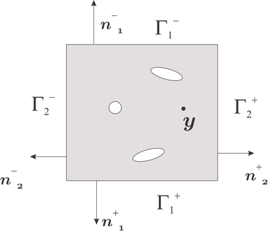
|
| Figure 3: RVE periodic domain, square cell. |
The different parts , , and of the boundary are represented in Figure 3. Considering the division on the boundary, we can re-express the fluctuation condition as
|
|
(2.31) |
where and represents the fluctuations in and . Similarly, and stands for the fluctuations in and .
Finally, considering the opposite direction on the normals defined in Figure 3, we end up with the periodic boundary conditions
|
More specifically, the fluctuation on the left part of the square cell must be equal to the fluctuation on the right part and, similarly, on the up and bottom part. Physically, this feature permits considering other micro-cell surrounding the RVE, and thus, the fluctuation will vary periodically along the micro-cell, hence its name.
Minimal boundary conditions. The minimum boundary conditions appear as the last alternative. They are considered the weaker boundary conditions since, in contrast to other boundary conditions, they assume no extra condition, hence its name. For this purpose, the fluctuation conditions (2.21) are imposed directly.
Note that fluctuation condition (2.21) leads to impose that the integral over the boundary of the open product between the fluctuation and the outward unit normal is zero. That implies to impose six conditions in 3D problems and three conditions in 2D problems.
Selected boundary condition and implementation strategy. The choice of the boundary condition is a priori arbitrary, and it would depend on the addressed problem. In our study, and throughout all this work, we select the periodic boundary conditions since they can ensure a representative volume with the smaller length scale .
Regarding the way to impose the boundary conditions, there are two options. On the one hand, it can be imposed directly in the equilibrium problem and consequently the Lagrange multipliers appear as extra unknowns. On the other hand, it is possible to condensate some unknowns on the system through the boundary conditions.
The first option seems reasonable for small number of conditions like minimum conditions, however, for other kind of conditions, it enlarges the system of equations considerably. The option of condensing the unknowns in periodic and linear seems reasonable. As a difficulty, if iterative solvers are used, specially for large 3D problems, the condensation process confers worse conditioning to the matrix, lengthening the convergence process. If direct solvers are used, with the condensation technique, the matrix becomes less sparse bringing problems with memory. This features that the appropiate approach will depend on the specific problem to be solved. In our case, and through all this work, since not computationally high demanding meshes are required, the condensation process is considered.
Strong form of the microscopic equilibrium equation. Once the boundary conditions have been introduced, the strong form of the microscopic equilibrium equation can be stated. From the equilibrium equation in weak form (2.17), and undoing the steps of integration by parts (and assuming some regularity), the equilibrium equation requires divergence free of the microscopic stresses. This is,
|
|
(2.34) |
To extend the formulation of the variational multi-scale method to microscopic equilibrium with body forces, the reader is refereed to work [7]. Thus, the strong form of the equilibrium equation jointly with the microscopic constitutive law (2.18) and the boundary conditions (periodic in our case) form the set of necessary equation of the micro-structural problem. Mathematically, it reads
|
|
(2.35) |
2.1.4 Homogenized constitutive tensor
Once the microscopic equilibrium equation is presented, it is worth mentioning that the main aim of the multi-scale problem consists in obtaining the homogenized constitutive tensor rather than the microscopic fluctuations, microscopic strains and microscopic stresses. In fact, computing the homogenized constitutive tensor is the essential part of the computational homogenization method. Henceforth, it is denoted by As in other fields of mechanics, it is commonly defined as the variation of the stresses with respect to the strain , this is
|
|
(2.36) |
Taking into account that the macroscopic stresses are related with its microscopic counterpart through the homogenization equation (2.16), and making use of the linear elasticity assumption (2.18), the constitutive tensor reads
|
|
(2.37) |
The microscopic strain is related with the macroscopic strain through the assumption of the kinematics described in equation (2.7). By taking derivatives with respect to the macroscopic strain in equation (2.7), we obtain the following relation
|
|
(2.38) |
where and stand for the identity fourth-order tensor and the so-called fourth-order localization tensor [8]. Unlike the homogenized fourth order constitutive tensor , both fourth order tensors and are dimensionless. Regarding this fourth-order localization tensor , note that, in the weak form of the equilibrium equation (2.24), the symmetric gradient of the fluctuations depends linearly (due to the assumption of linear material behavior) on macroscopic strain . Thus, we can relate with by writing the definition of the localization tensor as follows,
|
|
(2.39) |
Since the localization tensor stands for a linear operator, its components can be obtained by solving, for each canonical base of [2], the symmetric gradient of the fluctuation from the weak form of the equilibrium equation (2.24). Once the is known, replacing equation (2.38) on the definition of the constitutive tensor, the homogenized constitutive tensor is reduced to
|
|
(2.40) |
being and the volume average of the microscopic constitutive tensor and the fluctuation constitutive tensor. By definition, they take the following form
|
|
(2.41) |
Note that when the fluctuations are null (for example with Taylor boundary conditions), the localization tensor is canceled. Consequently, the homogenized constitutive tensor depends only to the volume average of the microscopic constitutive tensor . That explains why is commonly called the Taylor counterpart of the homogenized constitutive tensor. At this point, it is worth stressing that the whole homogenization process presented in this section is basically reduced to the homogenization of the constitutive tensor described in equation (2.40).
Note that all the formulation of the variational multi-scale method has been introduced under elastic regime assumptions. To extend this formulation to non-linear problem the reader is referred to [4].
2.2 Topology optimization
In the last decades, topology optimization has been a wide active research topic. Nowadays, it is widely applied to Aeronautical [9], automotive and civil engineering industry. In addition, topology optimization tools are nowadays included in more than thirty commercial software packages [1], e.g. Abaqus [10], Altair HyperWorks [11]. As an example, the design of the A380 ribs shown in Figure RealRib through topological optimization techniques represents a prominent application of the method in the Aeronautical industry.
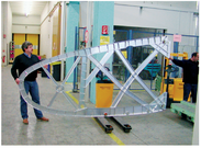
|

|
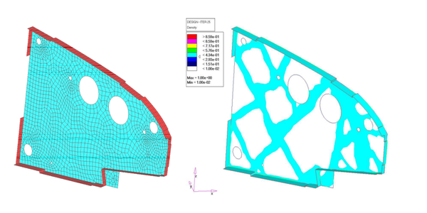
| |
| Figure 4: Topology optimization applications on aeronautical industry. The topology optimization fields is useful and developed enough for giving answers to real industry problems. | |
During these years of research and industrial development, different theories have been proposed. SIMP, shape optimization and topological derivative method are considered ones of the most convincing approaches.
The arguably most popular method, SIMP [1], is based on an heuristic regularization which leads to an appropriate (in terms of practical results) penalization. The root of this approach can be traced back to the seminal work [12] developed by Kikuchi and Bendsoe. In addition, due to this regularization, gradient-based methods can be used. However, although it can be sometimes interpreted in physical terms (micro-structures), intermediate values still appear and the selection of the penalization parameter is still an open issue [13]. This method has been successfully applied to material design in work [14] and to multi-scale topology optimization problems in the seminal work [15]. A more recent example can be found in work [16].
Boundary variation methods, based on classical shape sensitivity analysis, have appeared as a powerful alternative. Although shape differentiation has been long studied, the bases were established in the reference book [17]. The idea of using a level set method [18] for representing the topology is one of the strengths of the approach. The shape derivative is then used as a descend direction in a Hamilton-Jacobi equation which makes the level set evolves. Moreover, although strong mathematical theories have been developed, the inability of nucleating holes makes this approach limited.
Complementary, in the last years, due to the ever increase of the available computational power, discrete and evolutionary algorithms, like BESO [19], appeared as a clear way of defining interfaces in topology optimization. These methods, based in heuristics, offer the advantage that they are simple to code. However, they are limited to small cases and they are not computationally very efficient. For these reasons, they lack a great reputation in the topological optimization community [13].
In the last years, techniques based on topological derivative has become a significant tool for solving topology optimization problems. Its main merit is to provide sensitivity of the cost function when a small hole is created. The basis of topological derivative theory was first established in [20] by using the shape sensitivity results and then consolidated in the reference book [21]. Works [22] and [23] deserve also special attention. One of its main drawbacks, however, lies on the difficulty of obtaining such topological derivative, which can become in some cases burdensome. In fact, up to now, for some specific cost functions, topological derivatives are still missing. However, large advances have been achieved in the last years.
Owing to the landmark work [24], topological derivative can be used as a descent direction in a level-set algorithm. Slerp (spherical linear interpolation) algorithm has been used as an efficient strategy for solving topology optimization. It provides clear boundary of the topology and, in contrast with shape optimization techniques, the nucleation of the holes appears naturally.
2.2.1 The topology optimization problem
In the following, the topology optimization problem is stated under the assumptions of linear elasticity and small strains. Generally speaking, the aim consists of obtaining an optimal topology such that it minimizes a desired functional and satisfies some particular constraints.
The description of the topology is determined by the characteristic function as follows
|
|
(2.42) |
where the domain has been split into two parts . The sub-domains and are made of different materials, thus, the characteristic function is in charge of determining in the whole domain what part corresponds to either material. Such kind of problems are normally termed bi-material topology optimization problems. However, in most of the application, instead of dealing with two materials, the material corresponding to the domain is made of a very small stiffness characterizing the behavior of a void. The name of topological optimization problems usually refers to this case.
Regarding the cost functional, hereafter termed as , different options are possible. The compliance is widely used in the context of topology since it measures the stiffness of the structure. Other possibilities found in the literature are, for instance, the least square objective function [25], which attempt to achieve a certain displacement of the structure in norm.
Regarding the constraints, it is common to fix a desired volume of one of the materials, typically the strong one. In addition, it can be found, in works [26] and [27] of the literature, constraints imposing a threshold on the stresses. Perimeter constraints can also be found in order to alleviate numerical instabilities [28].
Concerning our work, we are interested in using the compliance as the cost function and the volume as the constraint. Accordingly, we state the topological optimization problem as follows,
|
|
(2.43) |
where is a general cost function (normally the compliance), the volume value to achieve, and the characteristic function. The cost function, in the case of the compliance, has the form
|
|
(2.44) |
where and represents the left hand side and the displacements solution of the following equilibrium equation
|
|
(2.45) |
where represents the bilinear form obtained by taking the weak form of the standard elastic problem
|
|
(2.46) |
The field stands for the stresses and stands for the constitutive fourth order tensor, usually defined in the bi-material problem as
|
|
(2.47) |
or, more explicitly, as
|
|
(2.48) |
where and are the constitutive tensor of the strong material and the weak material respectively.
2.2.2 Non-existence and numerical instabilities
In the topology optimization problems, some difficulties appear not only on the theoretical aspects but also on the numerical implementation. Regarding the theoretical aspects, we briefly describe the non-existence of optimal solutions by giving a representative example and we comment the standard remedies found in the literature. Regarding the numerical difficulties, we discuss the lack of unicity of the solution and the checkerboard instability.
Lack of existence of solutions
The existence of solution in topology optimization has been largely studied [29]. The question can be stated as: is there an optimal topology that minimizes the cost function and satisfies the constraints? This question is fully addressed [30] in the literature by providing some examples that show the non-existence of optimal solution. In the following, we are going to outline the counter-example described in book [29].
The aim lies on finding a topology that minimizes the compliance of a square domain under unit-axial loads.
Intuitively, the main idea consists in proposing a sequence of topologies with an increasing number of horizontal elliptic inclusions, smaller every time to preserve the volume. It can be seen that such sequence entails smaller compliance values. Since the sequence does not converge, the compliance value may always decrease. Thus, the optimal solution does not exist.
One remedy is to modify the problem by adding constraints. In several cases, it is very common to add a Perimeter constraint. In [28], it is shown how the Perimeter constraint may be used to limit the size of the inclusion. In addition, it can be proved with this Perimeter constraint, the existence of solutions is recovered. See works [31] and [28] for further information. Alternatively, it is also possible to introduce restrictions based on manufacturing issues to limit the size of the inclusions.
Lack of unicity
Besides the problems of existence, there are lack of unicity of solutions. In work [1], it is shown that one can get unicity of solutions if some specific regularizations of the problem are considered. However, most of the times, the obtained topology is full of gray regions and no physical meaning may be retrieved [13]. If this specific regularization is not considered, depending of the initial guess, several local minima may appear. This feature is due to the non-convexity of the problem. Thus, the initial value of the optimization problem influences on the optimal solution.
Checkerboard
In the context of topology optimization, it is well-known that, depending on the methodology, checkerboard solutions may appear. An intuitive way of understanding such phenomenon is writing the topology optimization problem (2.43) as a saddle point problem of two fields: the displacements and the characteristic function , this is
|
|
The checkerboard phenomenon usually appears, in other fields (e.g. Stokes flow), on problems. In that case, the Babushka-Brezzi condition must be satisfied. Similarly, in the topology optimization problem, the use of an appropiate interpolation of the displacement field and the characteristic function may circumvent the checkerboard problem. Alternatively, an other remedy for avoiding checkerboards may be the use of filters. A deep study on this topic is collected in work [32]. For further information, the reader is referred to works [32] and [33]. A representative example of the checkerboard phenomena is depicted in the standard Cantilever example of Figure 6.
![Checkerboard phenomena in topology optimization problems (figure extracted from [1])](/wd/images/thumb/9/9a/Draft_Samper_118254298-Checkerboeard.png/600px-Draft_Samper_118254298-Checkerboeard.png)
|
| Figure 6: Checkerboard phenomena in topology optimization problems (figure extracted from [1]) |
2.2.3 Regularized topology optimization (SIMP)
Regarding the different approaches to address the topology optimization problem, we start by describing the SIMP method. As it was mentioned before, the SIMP method is the most common approach in topology optimization. The origin of the methodology comes from the seminal paper of Kikuchi and Bendsoe[34]. It has been applied to many fields with success and it has produced hundreds of publications. Certainly, all the publications of Sigmund and its group has strongly contributed on giving useful solutions to real industry problems. The reference book [1] of Bendsoe and Sigmund, certifies that, nowadays, the SIMP method is considered by the topology optimization community, a consolidated theory.
The approach is based on regularizing the discontinuous characteristic function . Instead of taking values zero or one, the characteristic function is allowed taking intermediate values. Schematically,
|
|
where denotes the regularized characteristic function and it is usually termed fictitious density.
In addition, in order to get black and white topologies, the definition on the constitutive tensor in equation (2.48) is modified as
|
|
(2.49) |
where the parameter is arbitrary and leads to penalize the intermediate fictitious densities. Typically, in linear elasticity, the penalization parameter is taken as However, no penalization is considered in the volume constraint. It reads
|
|
(2.50) |
The fact that the constitutive tensor is penalized with the power of law and the volume is not penalized leads to stimulate the problem on choosing zero or one values of the fictitious density . Intermediate values are expected to increase the value of the volume with a non strong increase on the stiffness. However, depending on the problem intermediate values could appear with the inconvenient that not clear interpretation can be done. There are attempts to interpret it as an homogenized microstructure made of both materials but not always is possible (since it falls outside the H-S bounds).
The SIMP method, as an advantage, entails a straightforward implementation and provides satisfactory results. In addition, due to the penalization parameter , well-established and powerful continuous optimization algorithms can be used.
However the SIMP method also entails some inconveniences. The value of the heuristic parameter is unclear. In addition, in many cases, checkerboards may appear and filters must be applied. Finally, in the optimal solution, the fictitious density takes frequently intermediate values. As a remedy, there are two different options: either thresholding techniques are applied to recover “black-white” solutions or the intermediate values are interpreted, when possible, in terms of micro-structures.
2.2.4 Shape derivative for topology optimization
Another very popular approach for topology optimization consists in using the shape derivative concept. Many works have been developed in the last decades, specially by the french school [35] , [36] and [25]. The idea lies on collecting in the shape derivative the measure of the change of a functional when applying a deformation on the domain. In the case that, the deformation is applied on a boundary in the normal direction and with unitary modulus, the shape derivative can be straightforwardly computed, see [29]. Shape derivative has been obtained for several functionals like the compliance, volume and least squares cost functions, among others.
After the computation of the shape derivative, the optimality conditions have also been defined in the literature [29]. Since the change of the cost is collected by the shape derivative, it may be used as a descent direction in an optimization algorithm. This idea was pioneered by Allaire in the seminal work [25]. The topology is defined by a level-set function and it evolves following a Hamilton-Jacobi scheme. With this methodology, encouraging results have been achieved.
Since this methodology is based on a level set function, it is a priori free of grays (intermediate values) and no checkerboards are expected to appear. In addition, it relies on a strong mathematical theory.
As a main drawback, the shape optimization problem is restricted, by construction, to boundary changes, and consequently, no new nucleations of holes (or inclusions) are accomplished. However, some remedies has been proposed in [37] by combining the shape derivative and topological derivative.
2.2.5 Topological derivative for topology optimization
The field of topological derivative has gained an increasing popularity in the last decades. Although much of its success lies on the advances developed in the context of the shape derivative, it was not until the work of Solowski & Zochowski in 1999 [20], where the basis of the topological derivative theory were rigorously established. In parallel, Masmoudi presented the basis of the shape and topological derivative in [38]. Special attention deserves the previous works of Schumacher in [39] and [40] and Cea in [41]. Some years later, Novotny and co-workers at [42] presented and established a clear relation between the shape derivative and the topological derivative through the Eshelby tensor and connecting it with the configurational forces fully described in the reference book of Gurtin [43]. As a consequence of that studies, the reference book Topological Derivatives in Shape Optimization [21] emerged.
The topological derivative is based on the asymptotic analysis of shape functionals and the analytical solution of classical elastic problems of an infinite domain with an elliptic inclusion. The studies of Nazarov in [44] helped to consolidate the theory of the asymptotic analysis. Regarding the analytical classical solution of elastic problems, the books of Little [45], Muskhelishvili [46], Lekhnitskii [47] and Saad [48] are classical references.
All the progress on topological derivative theory leads to an extended number of applications which could be summarized in the following list
- Topological optimization: [49], [26], [50], [51], [52] and [53].
- Inverse problems: [54], [55], [56] and [57].
- Image processing: [58], [59], [60], [61] and [62].
- Fracture mechanics and Damage: [63], [64] and [65].
From the author's point of view, topological derivative is an adequate, and probably, the most natural tool for solving topology optimization problems since it studies the sensibility of a shape functional when making a hole (or inserting an inclusion).
It is worth mentioning that there are two different and complementary procedures to compute the topological derivative. The first one is based on studying the shape functional on two different configurations, with and without and inclusion. Then, after few manipulations, the differences of such functional are related with the topological derivative. The second approach, according to the reference book [66], takes advantage of the shape derivative by making use of standard continuum mechanics tools like the material derivative concept. In this approach, it appears naturally the Eshelby tensor and it has more the flavor of the configurational forces school. This approach helps to understand intuitively the physical meaning of the topological derivative.
A brief introduction to the shape derivative concept is the following (see Figure 7). Let's assume that a circular hole (or inclusion) on the unperturbed domain with a radius of value is nucleated (or inserted). Then, the shape derivative of the desired objective function must by computed by taking the material derivative of the functional with zero velocity field on the boundary of the domain and with unitary and normal velocity field on the circular hole. This shape derivative could be seen as a limit of a small perturbation of the radius of the inclusion (limit in in Figure 7).
Then, once the shape derivative is obtained (which itself involves a limit), we expressed it in terms of , or more specifically, in terms of powers of , mimicking a standard Taylor expansion. It is worth mentioning that the most relevant part of computing the topological derivative remains on obtaining this shape derivative in terms of power. This procedure is well-explained and detailed in chapter 4 and in Appendices 7 and 8, for both isotropic and anisotropic materials. Finally, by taking the limit, we recover the topological derivative expression.
In Figure 7, we sketch these ideas of taking limits respect to the radius variation (interpretation of the shape derivative) and respect to the radius itself (interpretation of the topological derivative).
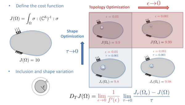
|
| Figure 7: Illustration of the topological derivative interpretation by passing the shape (variation of the radius of the inclusion ) and the topology (radius of the inclusion ) to the limit. |
In mathematical terms, the topological derivative is defined, more precisely, as the linear operator that fulfills the following expansion
|
|
(2.51) |
where and represent the domain with an without an inclusion. The term represents a circular inclusion in the point with a radius of value . Concerning the shape function , most of the times, it is taken similarly to the SIMP and shape optimization methods, i.e., the volume of the domain, the compliance of the structure or the norm difference between the displacement of a specific point of the domain with a displacement target value. However, the compliance functional plays usually a crucial role in the topological optimization problems. For this reasons, obtaining topological derivative of the compliance was an important stride in the topic of topological derivative. Specifically, the compliance shape functional is usually defined as
|
|
(2.52) |
where and represent the stresses and displacements solution of the standard elastic problem (2.46). Following Novotny in work [21], the topological derivative of the compliance is typically [21] presented in the following terms
|
|
(2.53) |
where stands for the fourth order polarization tensor. The expression of such polarization tensor, for the isotropic and anisotropic case, and the procedure to relate it with the topological derivative is fully explained in chapter 4.
3 Topological derivative and topology optimization
3.1 Motivation
As mentioned in Chapter 2, different methodologies are available to address the topology optimization problem. Certainly, the different formulations impact meaningfully on the numerical strategy proposed to solve the problem. For instance, the regularization of the characteristic function introduced in the SIMP method allows computing a continuous gradient. However, when using topological derivative, no continuous gradient is available. This difference results according to two significant considerations: on the one hand, standard KKT conditions are no longer imposed as optimality conditions; on the other hand, the usual continuous optimization algorithms (steepest descent, Newton Raphson, ...) must be replaced by alternative algorithms.
Regarding the optimality conditions, it is convenient to provide first an intuitive description of the topological derivative concept and, then, formalize it in mathematical terms. From that descriptions, the optimality conditions arise naturally.
The (non standard) topological derivative algorithm is also convenient to be described. The level-set updating, built to satisfy the optimality conditions, is not straightforward. In addition, this topological derivative algorithm becomes more complex when imposing constraints in the minimization problem, specially with inequality constraints.
Furthermore, the topological derivative algorithm presents two drawbacks of different nature. On the one hand, determining the line search parameter is not an easy task; significant oscillations appear leading to spurious local minima. On the other hand, for a threshold of the stopping criteria, the algorithm may not converge leading to time-consuming re-meshing processes. To alleviate both inconveniences, novel numerical strategies must be proposed.
3.2 Optimality conditions when using topological derivative
Once the topology optimization problem (2.43) has been stated in Chapter 2, the following question arises: how the optimality condition in the topology optimization problem must be imposed when using the topological derivative? Note that, strictly speaking, the topological derivative does not correspond to a continuous gradient, and consequently, non standard KKT conditions can be imposed.
3.2.1 Qualitative description of inserting an inclusion
For this purpose, an qualitative description of inserting an inclusion is first provided.
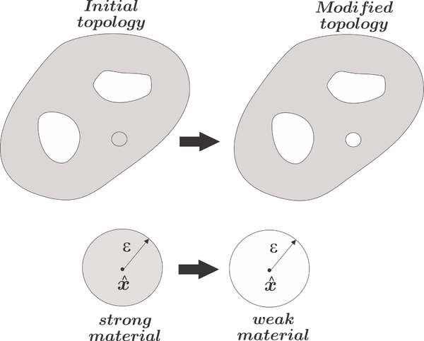
|
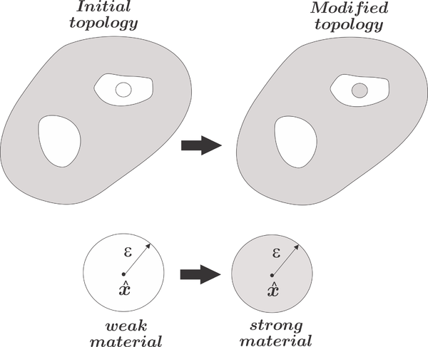
|
| Figure 8: Representation of the initial topology and the update topology for a strong-to-weak material modification (Case A) and for a weak-to-strong material modification (Case B). | |
Let's assume the domain is divided into two sub-domains: , endowed with a strong material (or material ) and , endowed with a weak material (or material –). In Figure 8, the strong material is represented in gray and the weak material in white. The main idea is based on studying how a shape functional (compliance, volume, ...) is modified when a circle of one material (strong or weak) is replaced by a circle of the other material (weak or strong). In an attempt to give a qualitative idea of this relation, the following two cases are introduced:
- Case A: when a small circle of the strong material is replaced by a small circle of the weak material, see Figure StrongToWeak.
- Case B: when a small circle of the weak material is replaced by a small circle of the strong material, see Figure 8a.
In this work, the shape functional is restricted to the compliance, denoted by , and to the volume (or mass in general), denoted by . In addition, we denote the shape functionals with and when the center of the inclusion is inserted in or respectively. Thus, the change of the shape functionals in both cases is as follows:
- Case A: Since the small circle made of the strong material is replaced by the weak material, i.e., to , the structure must behave less stiffer and, consequently, the compliance should increase as follows
|
|
(3.1) |
On the contrary, when is replaced by , the mass of the domain should decrease. This is,
|
|
(3.2) |
- Case B: Since the small circle made of the weak material is replaced by the strong material, i.e., to , the structure must behave stiffer and the compliance should decrease as follows
|
|
(3.3) |
On the contrary, when is replaced by , the mass of the domain should increase. This is,
|
|
(3.4) |
Thus, it can be inferred from this analysis the opposite response of the compliance and volume functionals when inserting an inclusion. In practice, this is translated to obtain solution different from the trivial one (full domain of strong material or full domain of weak material). In addition, this trend of the inequalities will incur on understanding the sign of the topological derivative.
3.2.2 Mathematical description of inserting an inclusion
Let's analyze, more formally, the mathematical formulation of inserting an inclusion. The circular inclusion is represented by means of the ball defined as
|
|
(3.5) |
where and stands for the center and the radius of the ball. The characteristic function on the ball centered in with radius as
|
|
(3.6) |
and the sign function as
|
|
(3.7) |
Bearing this in mind, a general description of the constitutive tensor from the initial topology to the modified topology (by only inserting one hole) can be mathematically expressed as
|
|
(3.8) |
Note that if (case A), the constitutive tensor changes from to in the circular inclusion and remains the same in the rest of the domain. An opposite behavior occurs in case B. Similarly, we express the change of the density from the initial topology to the modified one as
|
|
(3.9) |
3.2.3 Topological derivative of the volume
Let's express first the mass of the domain as the integral of the density over all the domain, i.e
|
|
(3.10) |
Note that, in fact, it represents the mass of the domain before inserting the inclusion. Equivalently, the mass of the domain after inserting the inclusion corresponds to
|
|
(3.11) |
By definition, see [67], the topological derivative holds in the following expansion,
|
|
(3.12) |
Hence, by identifying terms, we obtain straightforwardly the expression of the topological derivative for the mass (or volume) shape functional as
|
|
(3.13) |
Note that, for cases A and B, the topological derivative takes the following values,
|
|
(3.14) |
|
|
(3.15) |
3.2.4 Topological derivative of the compliance
In contrast to the volume functional, the compliance clearly depends on the constitutive tensor and is quite commonly expressed as
|
|
(3.16) |
where stands for the external boundary forces and represents the displacements, solution of the weak form of the equilibrium equation (2.46), i.e.,
|
|
(3.17) |
Note that the body forces are neglected for the sake of simplicity. Expression (3.16) corresponds in fact to the compliance of the initial topology of the domain. The difference between the modified topology and the initial topology is typically written, see work [21] and [68], in terms of the polarization tensor , as follows
|
|
where are the stresses, solution of (2.46). In the context of linear elasticity, they are described as . Thus, by identifying terms, the topological derivative is reduced to
|
|
(3.18) |
At this point, it is worth stressing that the polarization tensor has the following properties
|
|
(3.19) |
|
|
(3.20) |
The full expressions of the polarization tensor for both isotropic and anisotropic material are obtained in Chapter 4
As a summary of the variables and properties described so far, in Table 1, we show the initial and modified topology properties, the shape functional increments and the topological derivative for the Case A and B in a compact form.
| Case A (Strong to weak) | Case B (Weak to strong) | |
3.2.5 Optimality conditions
Once the topological derivatives are described for the volume and compliance and the topological optimization problem is stated, we present the optimality conditions of the topological optimization problem when using topological derivative. Let's assume that a shape functional (the compliance or the volume in our case) depends on a material parameter (the constitutive tensor or density) that takes values on and on . Defining an arbitrary direction as
|
|
(3.21) |
where determine an specific hole and the number of holes, we say, by definition, that is a local minimizer if, for any direction (and for any number of holes ), the shape function will always increase, this is
|
|
(3.22) |
If can be expanded asymptotically (the topological derivative exists), the difference of the shape functional is expressed, by definition, as
|
|
Thus, for small enough values , the necessary optimality conditions are set by imposing positivity on the topological derivative, i.e.,
|
|
(3.23) |
Accordingly, the topological optimization algorithm must fulfill condition (3.23). A similar description of the optimality conditions can be found in work [67].
3.3 The Slerp algorithm
The lack of continuous gradient, and consequently, of standard continuous algorithms (steepest descent, Newton...) gave rise to propose, as an alternative, the Slerp algorithm for solving topology optimization problems when using the topological derivative. We recall that it was resourcefully achieved by Amstutz and co-workers in the seminal work [49].
3.3.1 The level-set function
The methodology lies essentially on defining the topology via a continuous function, usually called level-set function. More specifically, the zero level of that function determines the characteristic function and, consequently, the topology. As a main advantage, this method allows obtaining complex and very different topologies by means of a slight continuous change of the level set function, as we can observe in Figure 9.
More formally, the characteristic function is defined on the domain usually by the level-set function as
|
|
(3.24) |
where represents the Heaviside function. Note that, owing to this definition, the design variable of the topology optimization problem switches, in practice, from to .
3.3.2 Optimality condition when using a level-set function
Let's now relate the level-set function with the optimality condition (3.23). The function is defined as the scalar function satisfying
|
|
(3.25) |
Hereafter, we will use or indistinctly when referring to the topological derivative. Thus, with this definition in mind, the necessary optimality condition (3.23) becomes as follows
|
|
(3.26) |
Consequently, both the level-set function (by definition) and the topological derivative function (in order to fulfill optimality conditions) satisfies
|
|
(3.27) |
In view of this result, one can set the optimality condition for the level-set function as
|
|
(3.28) |
Note that, since the topological derivative depends on the topology, and consequently on the level set, the above equation is highly non-linear.
3.3.3 Slerp algorithm for unconstrained optimization problems
From the optimality conditions of the level-set function, one can naturally impose parallelism between the level-set function and the topological derivative at the minimum, that is
|
|
(3.29) |
where . Note that this relation fulfills automatically the optimality condition (3.28) for the level-set function. One could think on using equation (3.28) in a fix-point algorithm to get the optimality conditions. However, since is an arbitrary parameter, the level set function can increase unlimitedly and, consequently, the algorithm may not converge. In order to mitigate such inconvenient, one could fix such that the level-set function is enforced to have unitary norm. Thus, by taking , equation (3.29) becomes
|
|
(3.30) |
This relation satisfies equation (3.28) and can be understood as a fix-point algorithm: given a topology through a level-set function, compute its topological derivative and, by normalizing it, obtain the new level-set function and, consequently, the new topology. However, this fix point method could be highly aggressive leading to no descent direction during the iterations.
As a remedy, instead of updating the level-set in terms only of the new normalized topological derivative, one could combine it with the previous value of the level set, in such a way that the updated level-set function has unitary norm. This strategy is, in fact, what the slerp algorithm proposes.
The name of slerp arises from the computer graphics community and is shorthand for spherical linear interpolation. Shoemake [69] introduced this concept in the quaternion interpolation context for the propose of animating 3D rotation. In the topological optimization context, the slerp algorithm was proposed by Amstutz in work [49]. Note that in the context of quaternion interpolations, the objects to be interpolated are vectors of dimension four while in the context of topology optimization, the objects to be interpolated are fields defined over the domain.
In general, the slerp algorithm can be understood as the interpolation of two different functions on the unit sphere. In Figure (10), we show schematically the relation between the new level set function , the actual level-set function and the topological derivative .
According to the triangle relation described in Figure (10), the following equation must hold
|
|
(3.31) |
where the scalar numbers and can be computed by imposing the following law of sinus
|
|
(3.32) |
Note that this last relation is fulfilled due to the unitary norm of , and . In Figure (11), we depicted that trigonometric relation.
Thus, the new level set function can be written as a combination of the actual level-set function and the topological derivative as follows
|
|
(3.33) |
where is a line search-like parameter and the angle between and which is written as
|
|
(3.34) |
Note that, an alternative way of imposing parallelism between the level-set function and the topological derivative s achieved by requires zero vale of the angle . In this respect, the stopping criteria of the algorithm can be set by imposing the tolerance as a threshold of the angle .
In addition, it is remarkable that, by using the slerp algorithm, the updated level-set function has automatically unit norm. Note that since , we have chosen the norm for both, the norm and the scalar product of equations (3.33) and (3.34). However, other norms (or ) can be used.
Moreover, the line-search parameter allows controlling the size of the step. Initially, it is usually set to and it is divided by 2 until the new topology provides a smaller cost function. Clearly, if takes unitary values, we recover the aggressive fix-point algorithm proposed in equation (3.30).
Thus, the slerp algorithm is a fix-point algorithm with a line-search parameter that interpolates in the unit sphere the actual level-set with the topological derivative. It is worth mentioning that the slerp algorithm can be seen in the optimization context as a standard steepest descent method with the particularity that the update variable must have unit norm. Consequently, the topological derivative plays the role of the gradient in the topology optimization problem, hence its importance. Although, in this work, an exhaustive numerical analysis has not been considered (see [70] for this purpose), one can expect linear convergence of the algorithm.
3.3.4 Slerp algorithm combined with an augmented Lagrangian scheme for constrained optimization problems
So far, we have described the slerp algorithm for unconstrained topology optimization problem. However, most of the applications require fulfilling some constraints. In this sub-section we present how to deal with the case of a volume constraint. To the author's knowledge, there is no a vast amount of algorithms to deal with constrained topology optimization problems when using topological derivative. The lack of continuous gradient undermine the possibility of using standard continuous optimization algorithms. However, the augmented Lagrangian algorithm is exempt of such limitation since it uncouples the update of the design variables (the topology in our case) and the update of the Lagrange multipliers [71]. Thus, in view of this property, the slerp algorithm can be combined with an augmented Lagrangian scheme in constrained topology optimization problems. The reader is referred to works [72], [73] and [74] for further information.
Equality constraints
Considering the level-set function as the design variable, the topology optimization problem with volume constraint (2.43) may be expressed as
|
|
(3.35) |
According to the reference book [71], and following the works [75,72,74], the augmented Lagrangian scheme for equality constraints proposes to solve the minimization problem (3.35) by introducing the following saddle point problem
|
|
(3.36) |
where is the Lagrangian functional, is the Lagrange multiplier and the penalty parameter. The augmented Lagrangian scheme is based upon solving the primal-dual problem sequentially with the particularity that an extra term is added in order to convexify the problem [71]. The algorithm considers first, a single (or multiple) iteration for minimizing the cost function and then a single iteration as
|
|
(3.37) |
for maximizing the cost function, i.e., an Usawa-like scheme [76]. Certainly, the augmented Lagrangian scheme has an impact in the slerp algorithm. On the one hand, the cost function is replaced by the Lagrangian functional when determining the line-search parameter . On the other hand, the topological derivative of the Lagrangian functional must be computed by considering an extended topological derivative as
|
|
(3.38) |
where stands for the topological derivative of the cost function ). Note that, the topological derivative of the volume constraint is equal to and has been consequently omitted. Hereafter, for simplicity, the extended topological derivative is also called topological derivative.
Inequality constraints The augmented Lagrangian scheme can be extended to minimization problems with inequality constraints. The main idea consists in retrieving the minimization problem with equality constraints by adding an extra variable , often termed slack variable, to the minimization problem with inequality constraints. In mathematical terms, it reads as
|
|
(3.39) |
where the constraint function has been defined. Then, following the augmented Lagrangian scheme for equality constraints, the augmented Lagrangian is defined and the following saddle-point problem
|
|
(3.40) |
must be solved. The procedure consists in imposing one of the KKT conditions to isolate the slack variable in terms of the design variable and the Lagrange multiplier , and then inserting its expression in the augmented Lagrangian . For this purpose, we enforce that the partial derivative of the Lagrangian functional with respect to the slack variable must be canceled. This is,
|
|
(3.41) |
The two possible solution of the above equation are written as
|
|
(3.42) |
In order to determine the solution that leads to a smaller augmented Lagrangian value, we first insert and into the definition of the constraint function as follows
|
|
(3.43) |
and then to the Lagrangian functional as
|
|
(3.44) |
|
|
(3.45) |
Comparing both Lagrangian functionals
|
|
(3.46) |
we obtain that solution always provide a smaller value of the Lagrangian functional. Thus, the optimal slack variable takes always value, provided of course that exists, this is when . Otherwise, the optimal slack variable takes the other solution . Therefore, it is useful to write the square of the optimal slack variable as
|
|
(3.47) |
or, more compactly, as
|
|
(3.48) |
By inserting this last result in the constraint function , we obtain
|
|
(3.49) |
where we have conveniently defined the constraint. Note that the problem no longer depends on the slack variable appears. Thus, the saddle-point problem for solving minimization problem with inequality constraints (3.40) becomes
|
|
(3.50) |
which represents a standard saddle-point problem for solving minimization problem with equality constraints (see equation (3.36)) with the particularity that the constraint depends explicitly on the Lagrange multiplier . At this point, it is convenient to examine if problem (3.50) can be treated as a standard minimization problem with equality constraints. For this purpose, the KKT
|
|
(3.51) |
are first imposed with slight abuse of notation. The is not strictly imposed on the topology optimization problem when using topological derivative. Instead, the optimality conditions (3.23) are considered. In any case, from equation (3.49) the and terms are determined as follows
|
|
(3.52) |
In addition, it can be shown that
|
|
(3.53) |
and, consequently, the product between these last two equations leads to the following result
|
|
(3.54) |
Thus, the KKT condition of the augmented Lagrangian with inequality constraint becomes
|
|
(3.55) |
which coincide with the KKT condition of the augmented Lagrangian with equality constraint when the the constraint is replaced by the constraint . This is,
|
|
(3.56) |
This last consideration extends the augmented Lagrangian scheme with equality constraint neatly to the inequality-constrained case. Thus, the Lagrange multiplier is updated in the same manner, i.e.,
|
|
(3.57) |
or, more explicitly,
|
|
It is worth stressing that this last equation shows how the augmented Lagrangian cancels the Lagrange multiplier when the inequality is not active. Likewise, the extended topological derivative is defined in the same manner of equation (3.38), i.e.,
|
|
(3.58) |
As an advantage, this scheme allows using the same implementation for both cases; equalities or inequalities; by means of exchanging the constraint with the constraint . For further information, the reader is referred to the reference book [71] for a rigorous description and work [72] for applying to topological optimization problem.
Penalty value and algorithm. It is worth mentioning that giving an adequate value to the penalty variable is not an easy task. In the reference book [71], it is suggested increasing the penalty during the iterations (when the constraint is not tightened enough). Similarly, in work [77], it is proposed to increase the penalty every five iterations. However, our experience shows us that the penalty cannot increase unlimitedly. A very small value of the penalty will make the problem converge very slowly but if, on the contrary, is very high the solution oscillates with the risk of non-convergence. So, as it was mentioned before, the appropiate value of this parameter will depend on the problem and on the sensibility of the cost when varying the constraint. The numerical experiments, further presented, suggest to normalize the cost function and take a small value of the penalty.
A detailed scheme of the Augmented Lagrangian Slerp algorithm is presented in Algorithm 1.
|
3.4 Treatment of the interface
The stresses and the topological derivative deserve special attention when dealing with the interface elements. In this section, we analyze an specific treatment of the interface elements in a bi-material elastic problem. Note that, although in topology optimization the aim is where to nucleate holes and where to leave material, in practice, the aim is how to distribute two materials, provided that the weak material takes significant lower stiff (usually times less).
3.4.1 Bi-material elastic problem
We proceed to examine how to deal with the bi-material problem, from the continuous and discrete point of view, and how the different treatments of the interface affect the cost and the topological derivative.
Formulation
In the bi-material problem, the domain is first divided in two parts, one sub-domain with a strong material and the other sub-domain with a weak material . Then, the classical form of the elastic problem (without considering, for simplicity, the body forces) is written as
|
|
(3.59) |
and by multiplying times the test function and integrating by parts, we obtain the weak form of the bi-material elastic problem as
|
|
(3.60) |
where the domain has been split into t and . Let's consider a a Finite Element discretization of equation (3.60). The domain is equipped with a conforming, triangular mesh composed of triangles , , and vertices , . Recalling the classical Finite element spaces, is the finite-dimensional space of Lagrange Finite Element functions, i.e. of affine functions in restriction to each triangle . A basis of is composed of the functions , , where is the unique element in such that if and otherwise. We take advantage of defining as the finite-dimensional space of Lagrange Finite Element functions on , i.e. of constant functions in restriction to each triangle . A basis of is composed of the functions , , where on and on , .
Thus, defining as the diameter of the triangles , the discretized displacement is the unique solution of the discretized weak form
|
|
(3.61) |
Let's split the domain into three different sub-groups: the elements (endowed with constitutive tensor), the elements (endowed with constitutive tensor), and the elements intersecting the interface that share both materials and are, for the time, denoted by the interface constitutive tensor . The different possible definitions of that interface constitutive tensor are further described and represents the main ingredient of the bi-material elastic problems. Bearing this in mind, we can define the regularized constitutive tensor as
|
|
(3.62) |
Consequently, the weak form equation (3.60), is re-written, after discretization, as
|
|
(3.63) |
The right side of the above equation has not been split into the elements because no it does not depend on the constitutive tensor.
Undoubtedly, the main difficulty of equation (3.63) relies on how to deal with the interface elements . Since we use Finite Element, the strains are element-wise constant and, consequently, the integration of the last term of the left hand side of 3.63 requires the value of on the Gauss points of the interface elements , in terms of material and . From definition (2.48), the regularized constitutive tensor on the interface is expressed in terms of the characteristic function as
|
|
(3.64) |
In view of equation (3.64), the description of the interface is based on the treatment of the characteristic function in the Gauss Points of the interface elements and, in turn, on the treatment of the level-set function . The characteristic function evaluated on the Gauss Points of the interface elements is, hereafter, termed as . For this purpose, two different approaches are commonly used in topology optimization when using topological derivative [49,78]: the In or Out approach and the P1-projection approach.
In or Out approach
The In or Out approach is based on taking the characteristic function on the interface in terms of the level-set function evaluated on the Gauss point . This is,
|
|
(3.65) |
Note that, in this case, the characteristic function on the Gauss point takes binary values, i.e.,
|
|
(3.66) |
Consequently, the constitutive tensor is restricted to and , i.e., it belongs to
|
|
(3.67) |
and, in terms of the level-set function, is written as
|
|
(3.68) |
P1-projection approach
Alternatively, a -projection approach can be considered. It consists on projecting the characteristic function from to the smaller finite-dimensional space , composed by the Finite Element functions . In mathematical terms, the -projection reads as
|
|
(3.69) |
where the values on the nodes are determined from the nodal level-set values , i.e.,
|
|
(3.70) |
Thus, since we are dealing with Finite Element functions, the value of the characteristic function on the Gauss point is reduced to
|
|
(3.71) |
where , and are the values of the characteristic function on the nodes and of the element . In the following, depending on the values of the level-set function, we examine the four different cases that may appear. Without loose of generality, we order the nodal values of the level-set function as follows: where , and are the position of the the nodes and .
Case A: All the values of the level-set function are negative and consequently all the values of the characteristic function are equal to , including the value on the Gauss point. This is,
|
|
(3.72) |
In fact, in this case, the element is not considered an interface element.
Case B: The value of the level-set function in the node is taken as positive whereas the nodes and remain negative. In this case, the value on the Gauss point becomes
|
|
(3.73) |
Case C: Similarly to Case B, the value of the level-set function in the nodes and are taken as positive whereas the node remains negative. In this case, the value on the Gauss point becomes
|
|
(3.74) |
Case D: Similarly to Case A, the values of the level-set function in the nodes , , and are taken as negative. In this case, the value on the Gauss point becomes
|
|
(3.75) |
In this case, the element is also not considered an interface element.
Note that, although the characteristic function has been regularized in all these cases projecting to , in practice, it can only takes the following four values
|
|
(3.76) |
and consequently, according to equation (3.64), the constitutive tensor on the interface is restricted to
|
|
(3.77) |
3.4.2 Mixed formulation approach
The main objective is to propose a formulation in which the interface constitutive tensor can change continuously when evolving the interface.
Formulation
The mixed formulation proposes to write both the equilibrium equation and the constitutive law separately in the weak form. Namely, find and such that
|
|
(3.78) |
where are the components of constitutive tensor and the body forces have been neglected for simplicity. The test functions are taken in and the test functions are taken in Let's recall that the finite-dimensional space and are composed by the and Finite Element functions and . Regarding the unknowns and , the displacements are discretized in Finite Element functions as and consequently the strains can be expressed as Finite Element functions . However, the stresses are directly expressed in Finite Element functions as .
Thus, in the interface elements , the second equation of (3.78) becomes
|
|
(3.79) |
Let's denote the volume of each interface triangular element and and the subdivisions with strong and weak material obtained when the level-set function cuts the element, see Figure 12.
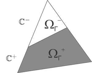
|
| Figure 12: The volume of the interface triangular element is divided into the sub-domains and with material properties and respectively. |
Since the Finite Element function takes, by definition, unitary values on , the above expression yields
|
|
(3.80) |
where it has been considered that the domain is split into and . Isolating the stresses from equation (3.80), the elementary constitutive law reads as
|
|
(3.81) |
Consequently, we can naturally define, in the mixed formulation approach, the constitutive tensor of an interface element as
|
|
(3.82) |
Note that in the rest of elements and , the standard relation between stresses and strains are retrieved.
Regularized characteristic function definition Then, we define the regularized characteristic function as the volume fraction of the strong material, i.e.
|
|
(3.83) |
where the value of will be determined by the zero level-set function. As a consequence of definition (3.83), we can identify the constitutive tensor of the fictitious material defined in equation (3.82) as
|
|
(3.84) |
Regularized characteristic function computation Following the description of the -projection, we again recognize, in the mixed formulation approach, the following four different cases for computing the regularized characteristic function:
Case A: Same as the projection approach. This is
|
|
(3.85) |
In this case, the element is not considered an interface element.
Case B: We start by computing the position of the cutting points and of the zero level-set function on the edges and (see Figure 13 ).
Since the level-set function is also defined in , the shape functions restricted to the edges become a standard 1D linear shape functions. It means that the level-set function over the edge can be written as
|
|
(3.86) |
where the linear shape functions and are defined as
|
|
(3.87) |
The cutting point is, by definition, the point in which the level-set function is zero and, consequently, from equation (3.86), it becomes
|
|
(3.88) |
Thus, the vector can be written as
|
|
(3.89) |
Similarly, the vector can be written as
|
|
(3.90) |
The weighted values and are conveniently defined as
|
|
(3.91) |
Then, taking advantage of the cross product, the fraction volume of the weak part can be computed as
|
|
(3.92) |
and after introducing equation (3.89), (3.90) and (3.91) yields
|
|
(3.93) |
and, consequently, the fraction volume of the strong part results in
|
|
(3.94) |
Thus, we end up with the expression of the regularized characteristic function of the mixed formulation in terms of the level-set function as
|
|
(3.95) |
Case C: In this case, we compute the regularized characteristic function in the same manner of Case B, only by exchanging node 3 by node 1 and the fraction volume of the strong material by the fraction volume of the weak material (see Figure 13). For this purpose, we can define conveniently the weights and as
|
|
(3.96) |
and the fraction volume of the strong part as
|
|
(3.97) |
Thus, in this case the regularized characteristic function of the mixed formulation in terms of the level-set function becomes
|
|
(3.98) |
Case D: Same as the -projection approach. The characteristic function takes zero value on the three nodes, i.e.,
|
|
(3.99) |
In this case, the element is not considered an interface element.
Comparison with other approaches In comparison with other approaches (In or Out or -projection approach), the characteristic function on the interface in the mixed formulation approach evolves continuously when moving the level-set function. Thus, the characteristic function is now defined in
|
|
(3.100) |
and, in trust, the constitutive tensor in the interface can also vary continuously from to , i.e.,
|
|
(3.101) |
In Table 2, we summarize and compare the treatment of the interface in terms of the characteristic function and constitutive tensor by the In or Out approach, -projection approach and the Mixed formulation approach.
| In or Out | -projection | Mixed formulation | |
Connections between the Mixed formulation approach and the Homogenization method
By examining equation (3.84), the interface constitutive tensor , defined in terms of regularized characteristic function , can be seen as a replacement of the black-white element by a gray element. More specifically, the material properties of the interface element is taken as a combination of the material properties of the strong and the weak material. Consequently, the interface element can be interpreted as an homogenized RVE with fraction volume . This is, in fact, the approach widely used by Allaire and co-workers in the reference book [3] for solving the topology optimization problem. Nevertheless, in that case, the regularized characteristic function is defined over all the domain. In order to avoid large gray areas, sophisticated techniques, like the perimeter constraint, must be considered in the homogenization approach. In contrast, we make use of the mixed formulation (or homogenization) only on the interface, with the advantage of getting black-white topologies in the major part of the elements and gray only in the interface elements . Thus, the proposed mixed formulation approach can be understood as a combination of the topological derivative approach on the domain and the homogenization approach on the interface.
With this homogenization technique, the interface elements have fictitious properties and no more purely black-and-white problems holds. However, two different compelling arguments encourage its use. On the one hand, from the physical point of view, the fictitious material with constitutive tensor can be interpreted as an homogenization of a micro-structure with fraction volume when Taylor boundary conditions are applied. See the multiscale sub-section 2.1.3 for further information. Thus, the regularized constitutive tensor corresponds to the homogenized constitutive tensor, i.e, , which can be understood in physical terms. On the other hand, from the numerical point of view, since the homogenization is only applied on the interface, as the mesh becomes finner, the gray interface measure tends to zero.
Connection between the Mixed formulation with the SIMP method
In addition, at this point, it is possible to relate the mixed formulation with the popular SIMP method. Instead of relating the regularized constitutive tensor with the regularized characteristic function linearly, as stated in equation (3.84), a polynomial relation can be used. Following the notation of Sigmund book [1], it is expressed as
|
|
(3.102) |
where the heuristic penalization parameter is usually set to .
From the physical point of view, the SIMP method does not always fulfill the Hashim-Strikman bounds [1] and, consequently, the regularized constitutive tensor can not be interpreted always as a homogenized constitutive tensor .
3.4.3 Treatment of the cost function and the topological derivative on the interface
At this point, the following question arises: how does the Mixed formulation affects the optimization problem, and more specifically, the cost and the gradient?
Implications of the mixed formulation on the cost function Regarding the cost function , we examine the implications of the mixed formulation when considering the compliance function. It can usually be written as the work produced by the external forces, i.e.,
|
|
(3.103) |
where the displacements are the solution of the standard equilibrium equation
|
|
(3.104) |
and represents the regularized constitutive tensor described in equation (3.62). Thus, the implications of the mixed formulation on the cost function rely completely on the behavior of the regularized constitutive tensor on the interface elements.
Implications of the mixed formulation on the topological derivative In order to study the implications of the mixed formulation on the topological derivative, we first examine the stresses . To simplify the notation, let's define the averaging operator as
|
|
(3.105) |
where and represent an arbitrary variable on the domain and Note that, on the definition of the regularized constitutive tensor on the interface, the operator has already been used as
|
|
(3.106) |
In addition, it can be observed that when the two first variables are equal, the averaging operator becomes the identity operator. This occurs in the case of the strains since they are constant in each element, that is
|
|
(3.107) |
Thus, the stresses on the interface are be computed as
|
|
(3.108) |
Following the definition (3.62), the stresses over all the domain will be computed as
|
|
(3.109) |
Note that, although the constitutive tensor is discontinuous inside the element, this formulation entails constant value of stresses inside the element. Bearing this in mind, we recall the standard expression, proposed in [66], of the topological derivative:
|
|
(3.110) |
In this last expression, dependency not only on the stresses but also on the polarization tensor are observed. Thus, following the regularization of the constitutive tensor , the polarization tensor can also be treated with the same operator in the interface. This leads to define the regularized polarization tensor as as in the elements , in the elements and in the elements , i.e.,
|
|
(3.111) |
Proceeding similarly, the regularized topological derivative , which is also element-wise constant, is defined as follows
|
|
(3.112) |
At this point, it is worth stressing the difference between computing first the topological derivative and then applying the regularization on the interface, with regularizing both the stresses and the polarization tensor and then computing the topological derivative. This difference only appears on the boundary and is written in mathematical terms as
|
|
(3.113) |
Since the topological derivative is the main ingredient of the optimization algorithm, it is convenient to be as accurate as possible on its computation. Thus, we choose for , instead of the described alternative, because it introduces only one regularization (instead of two).
For a better understanding, in Figure 14, we show how the material properties , and are evaluated in the interface elements . When an element is cut by the level-set into two sub-domains (black and white), we apply the average operator to the material properties, and consequently, the black-and-white element becomes a regularized element (gray) with interpolated material properties.
In Table 3, we summarize the values that the main variables of the topology optimization problem take in the strong material elements, in the weak material elements and in the interface elements.
| Constitutive tensor | |||
| Polarization tensor | |||
| Density | |||
| Displacement (with ) | |||
| Strains | |||
| Stresses | |||
| Compliance | |||
| Topological derivative |
3.5 Analysis of the Mixed formulation approach in topology optimization
In order to show the numerical improvements of the Mixed formulation on the slerp algorithm, we present the following two numerical examples:
- A singular triangular element example to analyze the implications of the Mixed formulation on the regularized characteristic function.
- A full domain example to analyze the implications of the Mixed formulation on the cost function and the topological derivative.
3.5.1 The mixed formulation approach in a single triangular element
Let's consider the interface triangular element delimited by the nodes , and represented in Figure 13.
The level-set function is defined in and its nodal values evolve following the given law
|
|
(3.114) |
where represents the level-set evolving parameter. Note that, it fulfills . By increasing parameter , the different cases described in sub-section 3.4.2 are retrieved. More specifically:
Case A
Imposing , the condition is fulfilled. In this case, since the level-set is all negative, the element is full of strong material.
Case B
The condition is satisfied by means of considering . In this case, an inner triangle of the weak material appears.
Case C
Considering , the nodal level-set function satisfies . In this case, an inner triangle of the strong material appears.
Case D
When , the level-set function is full positive, i.e. . In this case, the element is full of weak material.
The three different approaches (In or Out, -projection and Mixed formulation) described in sub-section (3.4.2 ) are used to compute the corresponding characteristic functions on the interface (, and ). In Figure 15, we represent the possible different characteristic functions when varying the evolving level-set parameter .
The In or Out approach, in comparison with the -projection approach, presents a more substantial discontinuity in the characteristic function when evolving the level-set function. However, in both approaches, the characteristic function behaves as a step function while the Mixed formulation presents a significant larger smoothness. Certainly, the proposed methodology allows obtaining a continuous variation of the characteristic function when evolving the level-set function.
3.5.2 The mixed formulation approach in a full domain example
Let's consider a x microscopic domain discretized with a regular mesh of triangle elements and the elastic parameters of the strong material defined as . The weak material takes a factor of the Young modulus and the same Poisson ratio. The level-set function is parametrized evolving level-set parameter as
|
|
(3.115) |
where and stand for the center of the circumference represented in Figure (16).
The evolving level-set parameter takes values in where and it is discretized in intervals. The proposed evolution produces a change of the circumference radius in the interval , large enough to advance up to more than an element.
The objective of the example is to examine how the Mixed formulation approach, in comparison with the In or Out and -projection approaches, affects the compliance, the volume and the topological derivative when evolving the level-set function.
Regarding the compliance, following equation (eq: compliance micro), it is defined as
|
|
(3.116) |
where the macroscopic stresses are taken as . In Figure 17, we can observe the different behavior between the compliance using the Mixed formulation approach and the compliance using the In or Out and -projection approaches. The Mixed formulation approach presents a continuous behavior whereas the In or Out and -projection approaches lead to discontinuities.
Regarding the volume, following equation (3.10), it is defined as
|
|
(3.117) |
In Figure 18, we can observe again that the volume using the Mixed formulation behaves continuously whereas the volume using the In or Out and -projection lead to discontinuities.
Finally, the topological derivative of the compliance in the node marked in Figure (16) is also considered. Following equation (3.112), it is defined in the Mixed formulation as
|
|
(3.118) |
and in the In or Out and -projection approach as
|
|
(3.119) |
Similarly, In Figure 18, we can observe again that the topological derivative using the Mixed formulation behaves continuously whereas the topological derivative using the In or Out and -projection lead to discontinuities.
Thus, it seems that the improvements of the Mixed Formulation on the regularity of the characteristic function shown in the last single triangular element example result in a significant improvements on the regularity of the compliance, volume and topological derivative, evidenced in this full domain example.
3.6 Element-to-node regularization of the topological derivative
In the Augmented Lagrangian Slerp algorithm detailed in Algorithm 1, an inconsistency appears in the update of the level-set function in equation (3.33). According to expression (3.110), the topological derivative depends directly on the stresses and strains, and consequently, is defined element-wise constant, this is, . Clearly, this kind of functions are not continuous which is, in fact, the requirement for updating the level-set function . Thus, updating the continuous level-set function can not be done by a combination of discontinuous element functions ( Finite Element functions in this case). As a remedy, a element-to-nodal regularization is considered.
Following the reference [79], it can be formulated in optimization terms as, find the unique such that it minimizes its difference with in norm. More precisely,
|
|
(3.120) |
Imposing that the Gateaux derivative of the functional on the direction is zero, we obtain
|
|
(3.121) |
where we have taken advantage of the symmetry property of the scalar product. Thus,
|
|
(3.122) |
The discrete form of the above equation can be rewritten as
|
|
(3.123) |
since the topological derivative is element constant. Rewriting the discrete continuous topological derivative in terms of the basis function , the in terms of the basis and taking as all possible basis function, equation (3.123) becomes
|
|
(3.124) |
which in matrix form is written as
|
|
(3.125) |
Note that the system of equation (3.125) has been solved by using the norm. Considering the norm is also possible. In practice, it consists on solving a similar system of equation by adding the stiffness matrix.
This element-to-nodal regularization has other names in the literature like least-square projection [79] or like Clément Finite Element interpolation [80].
Although certain accuracy is lost due to the smoothing operator, the level-set updating of the slerp algorithm, described in equation equation (3.33), is now possible.
3.7 Representative examples of the topological derivative for the macro-scale and the micro-scale
Before plunging into the details of the multi-scale topological optimization problem and in order to show all the tools explained until now, we present some results of the topological derivative approach applied to the macroscopic and microscopic topology optimization problems. On the one hand, it shows the capacity of the method. On the other hand, we can observe the behavior of the slerp algorithm when using the Mixed formulation.
3.7.1 Representative macroscopic example
As a representative macroscopic example, we focus on the Bridge example since it clearly shows the scope of the topology optimization techniques. In Figure 20, it is represented, on the left, the model to be solved by the topology optimization algorithm and, on the right, a real case solution.
Recalling the topology optimization problem, it is commonly stated on the macro-scale as
|
|
(3.126) |
where stands for the characteristic function and is the displacement solution of the bilinear form
|
|
(3.127) |
where the left and right hand side are given by
|
|
(3.128) |
where represents the external boundary forces.
According to Figure (20), the high and length of the domain is set to and . It is discretized by means of an unstructured mesh of Finite Elements. The parameter , and are taken as , and . The distributed force is taken unitary and the fraction volume , the penalty parameter as , the tolerance for the stopping criteria and the volume constraint tolerance . Regarding the material properties, the elastic parameters are , and the contrast parameter for the topological derivative is
Figure 21 shows different topologies obtained during the convergence process of the slerp algorithm. Certainly, the free-of-grays intermediate and final topologies evidence the suitability of using topological derivative in conjunction with a level-set function. In addition, the characteristic function presents no checkerboard instabilities.
| ||||||||||||
| Figure 21: Bridge topology optimization problem. Topology representation of the initial, intermediate and final iterations. Note the similarity between the optimal topology computationally designed and the topology proposed by the industry (shown in Figure 20). |
It is remarkable how the topological optimization solution takes only few minutes by a standard PC and looks very similar to the one in Figure (21).
3.7.2 Representative microscopic examples
Let's consider the micro-scale topology optimization problem as a second example to show the potential of the proposed methodology. The topology optimization problem is written as
|
|
(3.129) |
where is the RVE solid-volume, stands for the given unit norm macroscopic stress tensor and is the homogenized constitutive tensor defined in equation (2.40).
As a matter of example, three different cases are computed. In all of them, the initial topology is selected as in [27], the initial Lagrange multiplier is , the final solid-volume is , the elastic parameters are , the contrast parameter is and the penalty is chosen . The RVE is selected squared and it is discretized by a structured mesh of Finite Elements. The algorithm stops when and the volume constraint tolerance . The following three cases are studied (in Voight notation):
- Uni-axial horizontal stress-state:
- Shear stress-state:
- Bulk stress-state:
The obtained optimal topologies are presented in Figure Horizontal, shear, bulk.

|
| Figure 22: Horizontal, Shear and Bulk stress-state optimal RVE topologies |
The evolution of the compliance, the volume, the angle and the Lagrange multiplier along the iterations are depicted in Figure F_obj,theta,lambda,volum for bulk, horiz, shear.
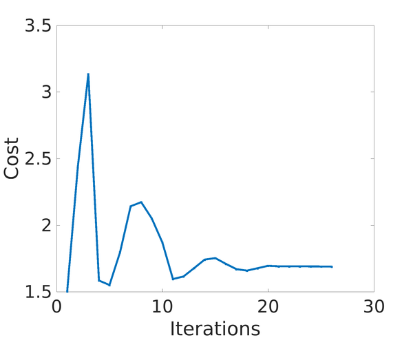
|
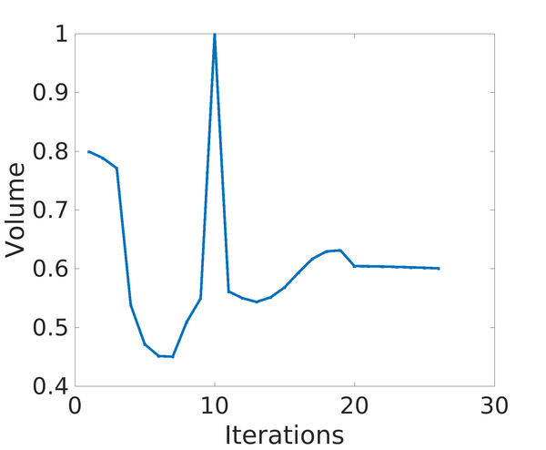
|

|
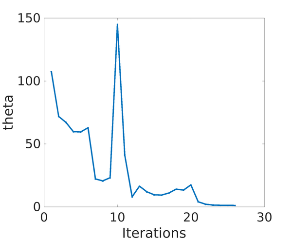
|
| Figure 23: Relevant information evolution along the iterative process | |
The presented curves show the standard behavior of the variables when solving a topology optimization problem.
Finally, in order to show the effect of the Mixed formulation on a real optimization example, we show in Figure (24) the behavior of the cost function in terms of the line search parameter in the first iteration of the Shear case when .
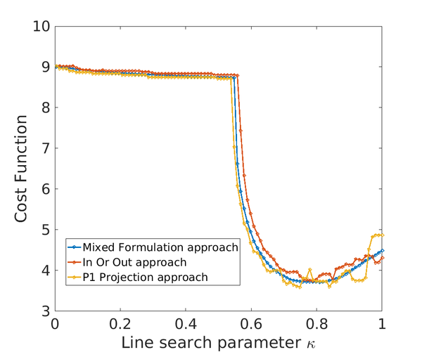
|
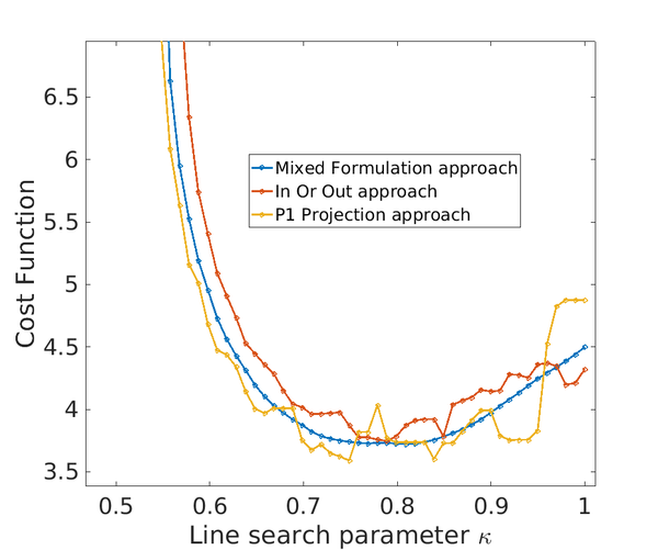
|
| Figure 24: The Mixed formulation, in comparison to In or Out and -projection, does not add spurious local minima when determining the line search parameter | |
Note that how the oscillations the In or Out and -projection introduce many local spurious minimums, making the line-search parameter difficult to determine.
In addition, as it has been mentioned before, the stopping criteria depends on the angle and, in turn, in the parallelism between the level-set function and the topological derivative . Since the level-set function is defined continuously , the discontinuity of the topological derivative when using the In or Out and -projection approaches introduces large values on the the angle , and consequently, difficulties on convergence, specially in cases with large variations of the topology (Bulk case). In the literature, see [49], this problem is alleviated by re-meshing. In contrast, the Mixed Formulation approach may obtain small values of the angle with no use of re-meshing. It is worth stressing that, in comparison with re-meshing, the additional computational cost when using the Mixed Formulation approach is negligible, only simple operations of the nodal level-set values must be computed. From the computational point of view, this fact represents the main contribution of the Mixed Formulation approach.
3.8 Summary and conclusions
As a summary, we outline the main work of this chapter. We have first introduced the optimality conditions for the topology optimization problem. Then, we have described the topological derivative for the macro and micro-scale in the case of isotropic materials, its mathematical and physical interpretation and the algorithm that must be used for solving the topology optimization problem. In addition, we have proposed the Mixed formulation approach as an alternative procedure of the interface treatment. Two numerical tests have evidenced the improvement on the continuity of the topology optimization variables. Additionally, we have also described the element-to-nodal operator necessary for using the topology optimization algorithm. Finally, we have presented a macroscopic and a microscopic numerical examples in order to show the behavior of all the numerical tools explained in this chapter.
As a conclusion of this chapter, in view of the two numerical test (level-set advancing in a single triangle and level-set advancing in a micro-structure domain), we can conclude that with the Mixed formulation , in comparison with the approaches presented in the literature, we have increased the regularity of the compliance, the volume and the topological derivative. As seen in Figure 24, this progress translates into two advantages: on the one hand, the choice of the line search parameter is exempt of spurious local minimizers; on the other hand, in contrast to other works in the literature, the re-meshing technique is no longer necessary to reach the convergence criterion . This fact represents the main contribution of this chapter. In addition, unlike the SIMP method, no additional parameter is required to solve the problem.
4 Topological derivative extension to anisotropic elastic materials
4.1 Motivation
Topological asymptotic analysis allows obtaining an asymptotic expansion of a given shape functional when a geometrical domain is singularly perturbed. This perturbation can be materialized by the insertion of holes, inclusions, source-terms or even cracks. The main concept arising from this analysis is the topological derivative [66]. This derivative measures the sensitivity of the shape functional with respect to the infinitesimal singular domain perturbation and it was rigorously introduced in [81]. Since then, this concept has proven extremely useful in the treatment of a wide range of problems; see, for instance, [82,83,84,85,86,87,88,89]. Concerning the theoretical development of the topological asymptotic analysis, besides the monograph [66], the reader is referred to [90,91].
In order to introduce these concepts, let us consider an open and bounded domain , see figure 25, which is subject to a non-smooth perturbation confined in a small region of size . Here, is an arbitrary point of and is a fixed domain of . Then, we assume that a given shape functional , associated to the topologically perturbed domain, admits the following topological asymptotic expansion [66]
|
|
(4.1) |

|
| Figure 25: Topological derivative concept. |
From (4.1), we obtain the standard definition of the topological derivative by passing to the limit :
|
|
(4.2) |
Notice that, since we are dealing with singular domain perturbations, the shape functionals and are associated to topologically different domains. Therefore, the above limit is not trivial to be calculated. In particular, we need to perform an asymptotic analysis of the shape functional with respect to the small parameter , i.e. we need information of when . As it was introduced in chapter 3, the shape functional difference (4.2) depends on the polarization tensor, which is considered a fundamental concept on the topological derivative topic. This tensor, also known in the literature as Pólya-Szegö polarization tensor, arises from the asymptotic analysis in singularly perturbed geometrical domains [92]. This mathematical concept permits to write an asymptotic expansion of the shape functional by means of functions evaluated in the unperturbed domain (without considering ). The polarization tensor is characterized by a matrix – polarization matrix – depending only on the constitutive properties of the problem and the shape of the singular domain perturbation [93].
The topological derivative, in its closed form, has been fully developed for a wide range of physical phenomena, most of them, when considering homogeneous and isotropic constitutive behaviors. In fact, only a few works dealing with heterogeneous and anisotropic material behavior can be found in the literature, and, in general, the derived formulas are given in an abstract form (see, for instance, [90]). Closed and analytical forms for this kind of constitutive behavior have been only developed for heat diffusion problems (see [94,95,96,81]). For anisotropic elasticity, the existence and properties of the polarization tensor was studied in [97,98]. However, the polarization tensor is given again in an abstract form. A technique for the numerical evaluation of the polarization tensor is presented in [99].
In what follows, we derive the topological derivative in its closed form for the total potential energy, i.e, the compliance, associated to an anisotropic and heterogeneous elasticity problem. We assume as singular perturbation a small circular inclusion introduced at an arbitrary point of the domain. The constitutive properties of the small disc are also anisotropic and different from the elasticity properties of the matrix. In addition, we provide a full mathematical justification of the derived formula, and develop precise estimates for the remainders of the topological asymptotic expansion.
Bearing this in mind, the heterogeneous anisotropic topological derivative concept, can be applied in advanced technological research areas such as topology and structural optimization simultaneously combined with topological material-design. In fact, in multi-scale modeling, for a given microstructure the homogenized constitutive response is, in general, anisotropic. In addition, since in each macroscopical structural point we have a different microstructure, the constitutive homogenized response at the macro-scale varies from point to point, i.e., it is heterogeneous. Therefore, for a correct evaluation of the topological sensitivity in a structural optimization problem, a derivative (the topological derivative) for an anisotropic and heterogeneous constitutive behavior is needed.
4.2 Problem formulation
The topological asymptotic analysis of the total potential energy associated to an anisotropic and heterogeneous elasticity problem is calculated. Thus, the unperturbed shape functional is defined as:
|
|
(4.3) |
where the Cauchy stress tensor is defined as usual:
|
|
(4.4) |
Note that the compliance differs from the total potential energy by a factor. Instead of the compliance, the total potential energy has been preferred to consider since it is more in accordance with the shape functional described in work [66].
In the above equations, is a symmetric fourth order elasticity tensor, is used to denote the symmetric part of the gradient operator and is the displacement field, solution of the following variational problem: find the field , such that
|
|
(4.5) |
In the variational problem (4.5) the space of admissible functions and the space of admissible variations are given by
|
|
(4.6) |
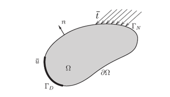
|
| Figure 26: Description of the problem. |
On the other hand, for our specific case, we consider a perturbation on the domain given by the nucleation of a small circular inclusion with constitutive properties given by a constant elastic tensor . Therefore, the perturbed shape functional can be written as:
|
|
(4.7) |
where the stress tensor associated to he perturbed configuration is defined as:
|
|
(4.8) |
Here, we consider that the inclusion is made of a completely different material. Then, the elasticity tensor can be written as follows
|
|
(4.9) |
In addition, in (4.7) the function is solution of the following variational problem:
Find the field , such that
|
|
(4.10) |
and both the set and the space are defined as
|
|
(4.11) |
where we use to denotes the jump of function across the boundary . Note that the domain is topologically perturbed by the introduction of an inclusion with complete different elastic constitutive properties (and in general anisotropic).
4.3 Topological derivative
Let us begin by choosing as admissible test function in problems (4.5) and (4.10), the function . Then, we obtain as a consequence the following expressions
|
Therefore, the shape functionals (4.3) and (4.7) can be written as
|
By considering the above results, the difference of the shape functionals and reads
|
|
(4.16) |
Taking into account the definitions of the perturbed elasticity tensor and perturbed stress tensor, we have that the difference of the total potential energy is given by an integral concentrated in the inclusion , namely
|
|
(4.17) |
with .
Let us assume that the elasticity tensor is smooth enough such that it admits an expansion in Taylor series around the point of the form , where . Now, in order to analytically solve the integral (4.17), we introduce the following ansatz proposed in [100] for the solution associated to the perturbed problem :
|
|
(4.18) |
where the function is the solution of the following exterior problem independent of the small parameter
|
|
(4.19) |
where , denote the fourth-order identity tensor and it was used the change of variable . The remainder in (4.18) must satisfy the following equation:
|
|
(4.20) |
which has the following estimate , with the constant independent of (see 4.4). The exterior problem (4.19) is solved explicitly in Appendices 7 and 8 for the isotropic and anisotropic materials. Some details are also provided in Sections 4.3.1 and 4.3.2. From Appendices 7 and 8, the stress tensor inside the inclusion can be written as:
|
|
(4.21) |
where and the fourth order tensor is determined again in Appendix 7 and 8.
Taking into account (4.18), the difference of shape functionals (4.17) reads
|
|
(4.22) |
where the term is given by
|
|
(4.23) |
which has the following estimate as shown in section 4.4. Next, by using the interior elliptic regularity of the function in , the difference of the shape functionals (4.22) satisfies the following identity:
|
|
(4.24) |
where the expansion of the tensor has been used again.
With the use of (4.21) and the change of variables the above expression can be analytically solved leading to
|
|
(4.25) |
where can be recognized as the Pólya-Szegö polarization tensor, given explicitly by
|
|
(4.26) |
Finally, using the definition (4.1) and taking , the topological derivative for the problem under consideration is given explicitly by
|
|
(4.27) |
Note that this formula is general, in the sense that, it measures the sensitivity of the total potential energy when two materials with completely different constitutive tensors are considered. Also, the polarization tensor depends only of the constitutive tensors and . This means that once defined and , for the point , the tensor can be easily obtained by computing the components of , see Appendices 7 and 8, and consequently so is .
From the final expression of the polarization tensor associated to the anisotropic and heterogeneous elasticity problem 4.26, we can analyze the limit case when the inclusion becomes a hole by taking the limit when . On the other hand, if we can analyze the sensitivity to the introduction of a rigid inclusion, we need to take the limit when . It should be noted that both limits exist and they can be easily obtained.
4.3.1 Exterior problem for isotropic materials
Although the topological derivative for isotropic materials in 2D plane stress has been obtained in many works [66], [101], from our point of view, it is not fully explained and we miss the description of some steps. In addition, in some works [66], the final expression is given by assuming that the Poisson ratio in the matrix and in the inclusion coincide. We present full steps of the procedure for computing the topological derivative and the closed expression for general values of the Poisson ratio. Similar expressions can be found in [93] and [102].
The aim and the key ingredient of obtaining the topological derivative lies on solving the following exterior problem
|
|
(4.28) |
where stands for an arbitrary second order tensor. According to (4.19), in our case, it becomes
|
|
Note that, precisely, the aim of the work lies on determining the expression of the polarization tensor In this section, we only give the necessary ingredients for computing the expression of the polarization tensor . In Appendix 7, all the steps for solving the exterior problem (4.28) are described.
Defining the real adimensional numbers and in terms of the constitutive properties and (background material), and and (inclusion) as
|
|
(4.29) |
the matrix can be written as follows
|
|
(4.30) |
The components of the matrix are related to the components of the tensor by the standard contracted notation (or Voigt notation) using the following rules for replacing the subscript:
|
|
(4.31) |
After solving problem (4.28), see Appendix 7, the stresses in the inclusion can be written, in terms of the tensor and consequently in terms of the stresses in the unperturbed domain as
|
|
where the fourth order tensor reads as
|
|
(4.32) |
In view of the symmetries of and , the tensor enjoys the following symmetry properties:
|
|
(4.33) |
Finally, after defining the fourth order tensor as
|
|
(4.34) |
we can, precisely, obtain the polarization tensor of equation 4.26 for plane stress as the following fourth-order isotropic polarization tensor:
|
|
(4.35) |
where
|
|
(4.36) |
|
|
(4.37) |
Note that, by considering , the parameters (with ), expression (4.35) becomes the polarization tensor for isotropy elasticity widely used in structural topological design [66].
As a remark, in order to recover the standard topology optimization problem, the material parameters of the strong domain are denoted by and and the parameters of the weak domain are commonly considered as and , where stands for the jump of stiffness. Thus, we consider two scenarios: first, considering an inclusion of the weak material (or void) inserted in the strong material () and the second one when an inclusion of the strong material appears in the weak material (). Consequently, rewriting the polarization tensor as , both cases enjoy the following properties
|
|
(4.38) |
Note that is a parameter small enough for modeling a void and large enough to entail invertibility properties to the stiffness matrix. Typically,
4.3.2 Exterior problem for anisotropic materials
In the case of anisotropic materials, a part from the work [99], there are no references that address the computation of the topological derivative closed-form. Similarly to the isotropic materials, we have to solve the following exterior problem
|
|
(4.39) |
where, in this case, the constitutive tensor has an anisotropic behavior in the inclusion and in the matrix. Since the polarization tensor can be obtained by equation (4.26), and the tensor by equation (4.34), the concerns lie on seeking matrix . The full details of solving problem (4.39) are described in Appendix 8.
By using the complex variable method, a final expression of matrix is obtained as
|
|
(4.40) |
where the logical matrices , , and are defined by
|
|
(4.41) |
and the complex matrices and by
|
|
In addition, the modified inverse constitutive matrix is defined as
|
|
(4.42) |
where the inverse constitutive tensor of the inclusion is expressed as
|
|
(4.43) |
The values , with , are the components of (in matrix notation). The real matrices and take the following expressions
|
|
(4.44) |
where and are the semi-axes of the elliptic inclusion. Since we are interested on circular inclusion, they are given by values
The product of the complex matrices deserves special attention. Due to some properties explained in Appendix (8), it can be written as
|
|
(4.45) |
where and take the real and imaginary part of the complex matrix which reads as
|
|
(4.46) |
and the complex numbers , , and are defined as
|
|
(4.47) |
Finally, the complex numbers and are the solution of the following characteristic equation
|
|
(4.48) |
and the complex numbers and are expressed as
|
|
(4.49) |
Unfortunately, the final expression of the matrix and the polarization tensor are cumbersome and can not be written explicitly. However, due to symbolic algebra, they can be easily calculated and saved as a computational function, ready for its implementation in a home-made topological optimization code.
Similarly to the isotropic case, we consider two scenarios: the case where the inclusion is inserted by a weak material on the strong one or the opposite case. Consequently, rewriting the polarization tensor as , both cases result to
|
|
(4.50) |
4.4 Estimation of the remainders
In this Section the estimation of the remainders in the topological asymptotic expansion is performed. This estimations has been used in the derivation of the topological derivative expression (4.27) presented in Section 4.3. In particular, we study the asymptotic behavior of the remainder in (4.20) and the residue defined in (4.23). Let us start by introducing the following lemma that ensures the existence of the topological derivative for the problem under analysis:
1: Let and be solutions to (4.5) and (4.10), respectively. Then, we have that the estimate holds true.
Proof 1: We start by subtracting the variational problem (4.5) and (4.10) to obtain:
|
|
(4.51) |
with . Now, by taking as test function in the above equation, we obtain the following equality:
|
|
(4.52) |
From the Cauchy-Schwartz and Poincaré inequality it follows that
|
|
(4.53) |
where we have used the elliptic regularity of function . Finally, from the coercivity of the bilinear form of (4.10), namely
|
|
(4.54) |
we obtain the result with the constant independent of the small parameter .
2: Let be solution to (4.20). Then, the following estimate holds true:
|
|
(4.55) |
with the constant independent of the small parameter .
Proof 2: From the ansatz proposed in (4.18) for and making use of the triangular inequality, we obtain:
|
|
(4.56) |
where we have used the change of variables , the equivalence between the semi-norm and the norm in and the estimate in Lemma 1. Finally, the results comes out from the Poincaré inequality.
3: Let and be solutions to (4.20) and (4.5), respectively. Then, we have the following estimate for the remainder in (4.23):
|
|
(4.57) |
Proof 3: From the Cauchy-Schwartz inequality we obtain
|
|
(4.58) |
Note that from problem (4.20) that the r.h.s. depends explicitly on the small parameter . Therefore, since this problem is linear and in view of Lemma 2, we can write . Then, we have
|
|
(4.59) |
which leads to the result.
4.5 Numerical validation of the topological derivative
The analytical formula for the topological derivative presented in (4.27), can be validated by using the following computational framework. Let's define (for a finite value of ) the function as:
|
|
(4.60) |
Clearly, the above definition has the following property,
|
|
(4.61) |
A numerical approximation of can be obtained by calculating the functions and , for a sequences of decreasing values of and, then, using (4.60) to compute the corresponding estimates for . The values of the function and are computed numerically by means of standard finite element procedures for the elasticity problem. The domain considered in the verification is a unit square (see fig. 27). The perturbed domains are obtained by introducing circular inclusions of radius
|
|
(4.62) |
centered at , with the origin of the coordinate system positioned at the bottom left corner. The finite element mesh used to discretize the perturbed domain contains a total number of elements and nodes.
To solve the anisotropic elastic problem, we prescribe the displacement on to be and traction on , (see fig. 27).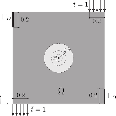
|
| Figure 27: Domain and boundary conditions. |
The study is conducted for four combinations of elasticity tensors and . The analyzed cases are detailed in the following box:
| Matrix constitutive tensor | Inclusion constitutive tensor | |
| Case A | ||
| Case B | ||
| Case C | ||
| Case D |
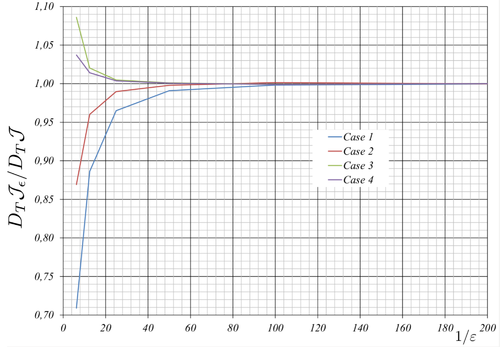
|
| Figure 28: Results of numerical verification. |
4.6 Representative Numerical Simulations
In order to assess the potential application of the topological derivative concept for anisotropic and heterogeneous materials, some numerical examples are shown in this section. All the examples are computed with the slerp algorithm described in the sub-section (3.3) and the Mixed Formulation technique described in sub-section (3.4.3). As it is commonly used, a minimum compliance objective function, subject to a certain fraction volume constraint, will be solved. To this end, the material distribution in will be identified by a characteristic function . Thus, the objective function can be written as a function of as: , where is used to denote the geometrical dependency of the domain on the characteristic function . Then, the optimization problem reads:
Find the characteristic function such that,
|
|
(4.63) |
where is the total potential energy of an standard elastic equilibrium problem (4.5) and the final intended volume. Note that the constitutive tensor can be heterogeneous and anisotropic. Some numerical examples with homogeneous and heterogeneous material distribution are considered. All them are solved below 2D elastic plane stress assumptions.
4.6.1 Homogeneous material distribution
The constitutive behavior is considered homogeneous in the design domain. Besides, the constitutive tensor in the inclusion is defined with the contrast parameter as: with . The 2x1 domain is discretized with a structured mesh of P1 triangular elements. The volume fraction is taken as and the penalty as . All the examples are stated to be converged when and . In the figures showing the results, the black and white colors are used to represent the part of the domain with constitutive tensor and , respectively. The elasticity of the inclusion is weak enough to mimic a void.
Case 1: Homogeneous Tension rod
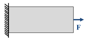
|
| Figure 29: Schematic drawing of a tension rod with homogeneous material distribution |
Notice the strong influence of the selected micro-structure topology and, consequently, of the resulting homogenized constitutive tensor, on the obtained optimal macro-structure topology.
Case 2: Homogeneous Cantilever beam
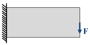
|
| Figure 31: Schematic drawing of a cantilever beam with homogeneous material distribution |
The isotropic case is used also as a reference. Some unconventional topologies are obtained, specially in the orthotropic case (micro-structure with horizontal and vertical bars) and full anisotropic case (last row). It can be observed, that the resulting macro-structure topology, tends to arrange following the principal directions of the micro-structure topology.
4.6.2 Heterogeneous material distribution
A heterogeneous distribution of material is used for a classical cantilever beam optimal design. The contrast parameter is taken . The 2x1 domain is discretized through a structured mesh of elements. The geometry is vertically partitioned in four domains with the same width (1/4). The top and bottom regions are endowed with a constitutive tensor different from the center one (see Figures 33 and 35). The intended volume fraction is and the considered penalty value is . Again the iterative solution algorithm is declared converged when and .
Case 1: Heterogeneous Cantilever beam with horizontal-shear micro-structures
In this example, the top and bottom regions are endowed with a microstructure topology yielding horizontally-dominant microscopic stiffness, where the center region, microscopic topology enforces shear-dominant stiffness.
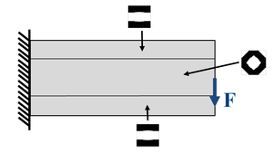
|
| Figure 33: Heterogeneous cantilever beam with regions of different constitutive properties (enforced via microscopic material topology). |
The material arrangement and distribution are sketched in Figure 33. The corresponding values for the resulting homogenized constitutive properties are detailed in Figure 34.

|
| Figure 34: Heterogeneous cantilever beam. Material properties and obtained results (case 1). |
It is worth noting that both constitutive tensors are again anisotropic. In addition, note that the optimal topology with the anisotropic heterogeneous material distribution is quite different from the homogeneous isotropic case (first row of Figure 32) and the homogeneous anisotropic case (last row of Figure 32). Again, it can be observed that the macroscopic topology tends to mimic the microscopic one in the different considered regions.
Case 2: Heterogeneous Cantilever beam with horizontal-vertical micro-structures
Now the top and bottom regions at the beam are endowed with a microstructure yielding horizontally-dominant elastic stiffness, whereas the central region is endowed with a vertically-dominant one.
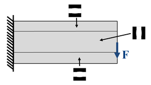
|
| Figure 35: Heterogeneous cantilever beam. Material properties and obtained results (case 2) |

|
| Figure 36: Optimal heterogeneous Cantilever beam topology. Constitutive tensor value and its corresponding micro-structure representation are also detailed. |
In Figure 36, the resulting (non trivial) optimal topology obtained for this case is shown.
Regarding numerical aspects, problems of convergence of the involved numerical schemes have not been found.
Besides, no substantial differences, in terms of the involved computational effort, have been found by considering the isotropic and anisotropic cases. Thus, the anisotropic topological derivative generalize the isotropic one. In all cases less than five minutes of computation are needed with a standard PC (3.40GHz processor in a 64-bit architecture) in a Matlab environment.
4.7 Conclusions
In this chapter an analytical and closed-form expression for the topological derivative in heterogeneous and anisotropic elastic problems has been presented. We consider as singular perturbation the introduction of a circular disc, with an anisotropic constitutive tensor completely different from the background material, in an arbitrary point. From the asymptotic analysis, it has been proven that the heterogeneous behavior of the material properties does not contribute to the first order topological derivative. The polarization tensor for this problem is obtained from a very simple (and inexpensive) matrix evaluation, in terms of the constitutive properties of the unperturbed problem and the inclusion. The derived formula are general for any kind of anisotropy in two dimensional problems, where orthotropy and isotropy (of the background material or the inclusion or a combination of both) can be derived as particular cases.
We recall that the development presented in this work for the total potential energy, in particular the solution of the so-called exterior problem, can be applied for other cost functionals and that the derivation of the associated topological derivative can be easily done.
With theses results in mind, the presented numerical simulation shows that the selected material properties heavily affect the optimal topology in an standard topology optimization problem. Since real applications involve non homogeneous isotropic material, the obtained closed formula of the topological derivative for heterogeneous anisotropic materials generalizes the concept of topology optimization for any kind of material properties and distribution. This progress is, in fact, the main contribution of the chapter.
In addition, a the influence of the microscopic topology on the optimal macroscopic topology is observed which, in some cases, becomes very relevant.
5 Two-scale topology optimization
5.1 Motivation
Let's recall the macroscopic and microscopic topology optimization problems.
Macroscopic topology optimization
Macroscopic topology optimization corresponds to the standard and genuine topology optimization problem. It aims at removing material from a macroscopic domain, subjected to external forces and boundary conditions, so that its stiffness is maximized. Usually, the problem is written as:
|
|
(5.1) |
where stands for the stresses, solution of a standard equilibrium equation, for the characteristic function, for the fraction volume and for the constitutive tensor.
In Figure 37, a representation of the macroscopic domain in the initial configuration and a representation of the optimal topology of the standard Cantilever beam is shown.

|
| Figure 37: Standard structural optimization solution for the Cantilever beam case |
Microscopic topology optimization
A similar approach is applied in microscopic topology optimization. The main idea, in this case, is to design the topology of the the RVE in order to maximize the stiffness obtained by the constitutive tensor so that a particular fraction volume is fulfilled. The reader is referred to [103] for some examples. Usually, the microscopic topology optimization is formulated as
|
|
(5.2) |
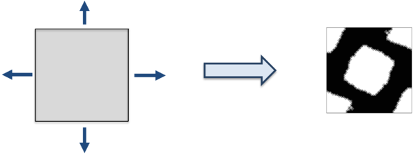
|
| Figure 38: Material design solution of a square micro-cell under a given stress state |
The multi-scale methodology, jointly with the microscopic topology optimization problem (both fully explained in Chapter 2), opens up the possibility of increasing the global stiffness via the topological design at the microstructure in each integration point. Hereafter, this problem is termed Point-to-point material design problem. It is worth stressing that conceptually the Point-to-point material design problem differs from the macroscopic topology optimization in the set of design variables. In the former, the macroscopic characteristic function is used as a design variable; while the latter uses the microscopic characteristic function .
At this point, from the numerical point of view, many questions arise: how the Point-to-point material design problem can be solved? What kind of algorithm should be used? In comparison with the macroscopic topology optimization problem, how much is the cost function reduced?
Since the Point-to-point material design involves multiscale and topology optimization techniques, significant time-consuming computations are expected. Additionally, as will be discussed later, the problem presents strong non-linear behavior. How can these difficulties be mitigated? Appropriate reduction techniques and algorithms are required. On top of this, the manufacturability issue appears as another relevant concern. For this purpose, appropiate numerical strategies must be devised.
Finally, instead of comparing the Point-to-point material design approach with the macroscopic topology optimization approach, a more stimulating strategy would be a combination of both approaches to increase even more the stiffness of the structure. In mathematical terms, it would consist in considering the macroscopic characteristic function jointly with the microscopic characteristic function . Similar questions arise: how this problem, hereafter termed Point-to-point multiscale topology optimization problem, can be solved? What kind of algorithm should be used? In comparison with the macroscopic topology optimization and the Point-to-point material design, how much the cost function is reduced? How the time-consuming difficulties and nonlinearities are alleviate? How manufacturability constraints can be considered?
5.2 Point-to-point material design problem
In order to shed light to the posed questions, we introduce first the Point-to-point material design problem. Conceptually, it makes use of the computational multi-scale homogenization framework and the micro-structure topology optimization technique. More specifically, it attempts to determine the optimal micro-structure topology at every point of the macro-structure domain such that a macroscopic functional is maximized (see a representative sketch in Figure 39).
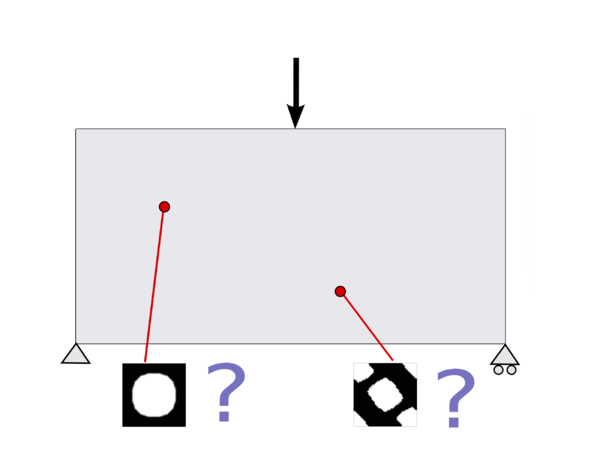
|
| Figure 39: Point-to-point material design problem |
Here the classical single-scale problem of determining the optimum distribution of a certain material mass at the macro-scale (or structural scale) is reformulated as a two-scale problem in the following sense: the goal is the optimal distribution of a given material mass, but now at the micro-scale level for every structural point (given the shape and topology at the structural scale).
5.2.1 Formulation of the Point-to-point material design problem
The Point-to-point material design is mathematically stated through:
|
|
(5.3) |
where the macroscopic stresses are defined by
|
|
(5.4) |
and are the displacement solution of the equilibrium equation.
In equation (5.3), , refers to the characteristic function at the RVE, whose optimal spatial distribution (defining the topology of the RVE) is aimed at being obtained, and refers to the volume fraction of the RVE. In this respect, the following aspects, specific for this multi-scale problem, have to be highlighted:
- The objective function to be minimized is highly nonlinear and defined at the macro-scale level.
- The design variables (the values of the characteristic function ) are defined at the micro-scale
- The equilibrium equation couples both macro and micro levels since, although the stresses are defined at the macrostructure, the constitutive equation (5.4) depends on the micro-structural topology.
- Since the number of design variables will be, in the discrete sense, of the order of the product of the macroscopic Gauss-point and microscopic Gauss-points (each RVE must be designed), the optimization problem may become computationally unaffordable.
Note the slightly but essential difference formulation between the Point-to-point material design problem, described in equation (5.3), with the macroscopic topology optimization problem, described in equation (5.1). The macroscopic characteristic design variable turns into the microscopic characteristic design variable .
Algorithmic separability As pointed-out above, the addressed minimization problem in equation (5.3) entails multi-scale coupling and non-linear dependencies. A separation of the minimization problem is introduced here to overcome those difficulties. The original problem in equation (5.3) is rephrased as:
|
|
(5.5) |
This subtle change could be thought as a different notation of the same problem or, even more stimulating, a way of solving the problem. Once in that stage, and inspired by the divide and conquer approach, a tentative second step consists of solving the minimization problem locally, i.e., rewriting equation (5.5) as,
|
|
(5.6) |
where the leading change is the exchange between the minimization and the integral operator. Note that the equilibrium equation plus the boundary conditions are solved as a standard FEM equilibrium problem, that is,
|
|
(5.7) |
Since all the unknowns and constraints of the minimization subproblem are defined locally at equation (5.5), the exchange can be done without altering the global solution. In other words, the micro-scale topologies that provide the minimum global (structural) compliance, are those micro-structure topologies that provide minimal “local compliances”.
Algorithmic complexity The algorithmic complexity (here understood as the number of operations to be performed) is tackled by considering a typical FEM discretization, involving, say, finite elements at every scale and design variables ( values of the characteristic function at the RVE, times macroscopic sampling points). Hence, one optimization problem with a total of design variables has to be solved.
In contrast, problem (5.6), may be seen as a local design-variable optimization problem, solved times (one for every macroscopic sampling point). This makes an enormous difference in terms of the problem complexity and the corresponding computational cost.
With this new strategy, the local optimization problem is then sought, as iteratively solving the global equilibrium equation, starting with a given initial micro-structure topology distribution, and modifying it by a microscopic topology optimization algorithm leading to a new RVE topology (in an uncoupled way from the other RVE's), until convergence. Thus, a natural strategy to solve the problem consists of solving each local optimization in a parallel fashion, or, in other words, with these approach, the problem becomes embarrassingly parallel. A similar approach is presented in [104].
5.2.2 Vademecum-based approach for computational cost reduction
Despite resorting to parallel computation, problem (5.6) still exhibits high complexity and it becomes computationally unaffordable for real-life problems. For this scenario, a more efficient approach is proposed here. The main idea consists of optimizing a priori a very large discrete-set of micro-structures, in the set of possible macro-stresses acting on the RVE, leading to the so-called Material Catalogue or Computational Vademecum [105]. Then, when in the Point-to-point material design problem a certain optimal microstructure topology is requested, for a given stress-state at the macro-scale sampling point, the Vademecum is consulted and the closest optimal solution is extracted.
More precisely: given the mechanical properties of the base-material, the expensive computations requested for the Vademecum construction are done once-for-ever, in an off-line step, and the Vademecum outputs (typically the homogenized constitutive tensor, , solution of equation (3.129), are stored in a data-base for, a sufficiently large, discrete set of entries
The actual multi-scale material design problem is then performed on-line, and it only involves a recursive equilibrium analysis at the micro-scale combined with consultations of the Vademecum. This translates into an impressive reduction of the computational cost of the on-line material design process. It is highlighted that the Vademecum remains the same for a given base-material, independently of the macro-scale structural problem aimed at being optimized.
Parametric domain description The parametric domain defines the range of the the space of all possible macroscopic stresses . Inspection of equation (5.6) shows that the modulus of does not play any role in the determination of the optimal RVE topology. In fact, it can be readily proven that
|
|
(5.8) |
Therefore, is the actual Vademecum entry. For 2D cases, the relevant entries are then made of unit-modulus stress vectors, which lie in the unit-radius sphere and can be parametrized in terms of the two Euler angles, and . This is,
|
|
(5.9) |
Hence, the parametric domain is represented by the unit radius sphere. Each point of the sphere can be seen as a micro-structure optimization case, which returns some homogenized elastic properties associated to an optimal topology (see Figure 41).
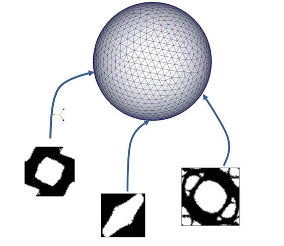
|
| Figure 41: The unit-radius spherical parametric domain (Computational Vademecum) |
Parametric domain discretization For the subsequent examples, the sphere has been discretized by means of a structured mesh of 16386 points. However, the bottom half points need not to be computed because they have an homologous point at the top half of the sphere. This is because or , plugged in problem (5.8), result in the same objective function. Besides, only a quarter part of the top half of the sphere must be computed due to symmetries and mirroring. Consequently, an eighth of the whole sphere has been actually considered for the computations, resulting into 2145 points to be actually computed. It is also noticeable that every case/point is fully uncoupled from the others and, therefore, the Vademecum construction is optimally parallelizable in a distributed memory computer cluster.
By the use of the topological derivative and the Slerp algorithm fully explained in Chapter 3, some examples of this optimal RVE topologies can be seen in Figure 42.
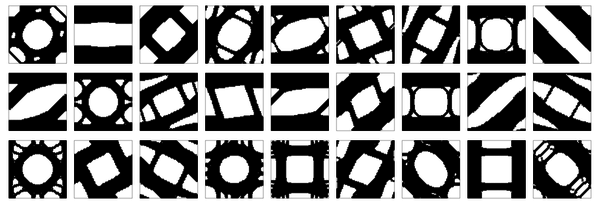
|
| Figure 42: Typical micro-structure topology outputs of the Computational Vademecum |
All the microscopic topologies have been computed fulfilling a solid volume fraction . It is worth mentioning that construction of such Vademecum requires a very robust methodology for the RVE topological design, so that, without the use of re-meshing, none of the desired entry points fails to be computed. In this sense, it has to be remarked that these results are obtained thanks to the use of the topological derivative concept, the Slerp algorithm and the Mixed Formulation (see Chapter 3). All cases converged for a constant value of the penalty , with a convergence tolerance and a tolerance on the volume constraint . In Figure 43, we show the structured mesh with 6400 linear triangle elements.
|
| Figure 43: Structured mesh used in the micro-structure topology optimization problem with 6400 standard linear triangular elements. Note that, the Slerp algorithm jointly with the Mixed formulation explained in Chapter 3 has converged in 2145 cases without considering re-meshing techniques. |
It is also remarkable from Figure 42, that, for many cases, the obtained optimal topologies are far from being intuitive. Associated to the optimal topologies, and based on problem (5.8), the corresponding RVE compliances for every point of the parametric space are computed, and they are displayed in Figure 44.
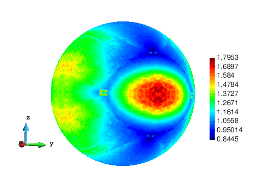
|
| Figure 44: Optimal compliance values over the parametric domain |
It has to be emphasized that, from the theoretical point of view, achieving a global minimum in all cases is not guaranteed, although numerical experiences have evidenced that the obtained compliances remain similar when changing the initial guess.
As explained in Chapter 2, the homogenized constitutive operator, , constitutes the relevant output of the Vademecum since this is the only data retrieved from the micro-scale to the macro-scale computations (see equation (5.8)). Accordingly, in Figure 45, the Vademecum outputs for the optimal homogenized components of are presented.
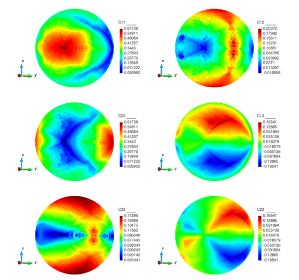
|
| Figure 45: Maps of the constitutive tensor components on the unit-radius spherical parametric domain. |
There, the major symmetries of (symmetric character of the maps of the symmetric components) as well as the rotated mirroring - and - can be observed.
5.2.3 Algorithm for the Point-to-point material design
The strategy of the problem relies on the alternate direction algorithm, widely used in literature, see [106]. We explain carefully the details in Algorithm 2.
| ||
|
Algorithm. 2 Alternate directions algorithm for the Point-to-point material design problem. |
5.2.4 Numerical results of the Point-to-point material design problem
In order to assess the proposed approach some numerical examples are presented next. In all cases the solid volume fraction at the RVE is fixed to . As start point in the iterative process, a micro-structure with a centered circular void fulfilling the volume fraction constraint is considered over all the macroscopic domain (see Figure 46-(a)).
Cantilever Beam The Point-to-point material design approach is first applied to the Cantilever beam example shown in Figure 46. The dimensions are 2 meter length 1 meter height, and plane stress conditions are assumed. The beam is loaded by a unit vertical point force, at the right end center, and it is clamped at the left end.
This rectangular macroscopic domain, is discretized into triangular elements. The elastic properties of the basis material are: Young Modulus and Poisson ratio . In Figure 46, the evolution of the micro-structure topology, along the iterative design process is displayed.
In Figure 47, the evolution of the global cost function (structural compliance) and of the residue (in terms of displacements) of the alternate directions algorithm is depicted. As it can be checked there, four iterations suffice to achieve full convergence with a 30% reduction of the original compliance. The convergence ratio of the iterative process is at most linear, as expected from the used alternate directions algorithm.
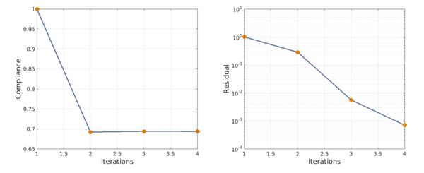
|
| Figure 47: Compliance and residue evolution of the alternate directions algorithm applied to the Cantilever beam example solved by the Point-to-point material design approach. |
Bending Beam The Point-to-point material design approach is now applied to a standard supported Bending beam. The same macroscopic domain is now discretized in linear triangular elements. The beam is loaded with a vertical unitary force at the mid-span (see Figure 48). The elastic properties of the basis material are: Young Modulus and Poisson ratio .
The evolving micro-structure distribution during the iterative design process is depicted in Figure 48. In Figure 49, a fast convergence is achieved also in this case (six iterations) leading to almost 40% reduction of the structural compliance.
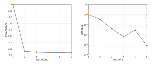
|
| Figure 49: Compliance and residue evolution of the alternate directions algorithm applied to the Bending beam example solved by the Point-to-point material design approach. |
Note that, due to the Computational Vademecum, these two numerical examples have been solved in less than one minute of computation with a standard PC (3.40GHz processor in a 64-bit architecture) in a Matlab environment.
5.3 Component-based approach for material design problem
One may argue that alternate direction algorithm 2 theoretically solves the Point-to-point material design problem (5.6). However, the results of the Point-to-point material design approach present relevant manufacturing limitations. Designing the material of a structure which has different micro-structure point to point seems unrealistic. Since this work aims at presenting clear realistic results, some additional constraints in problem (5.6) are now considered. It gives rise to the hereafter termed Component-based material design problem.
5.3.1 Formulation of the problem
In order to establish such manufacturing constraints, the macro-structure is divided in several sub-domains and a constant micro-structure is imposed in each sub-domain. In optimization terms, it can be cast as,
|
|
(5.10) |
where stands for the volume of each sub-domain ( ) . Figure 50 depicts roughly how the Point-to-Point material design problem becomes the Component-based material design problem.
In this approach, it is supposed that the partition of the domain is provided by the user depending on its interests and manufacturing capacities. Nevertheless, aeronautical industry, among others, trusts on first producing by components and then assemble them. Thus, each component is build and manufactured independently and the partition of the domain is straightforwardly decided (each components stands for a sub-domain). In Figure 51, a representation of the component-based manufacturability is shown.
From the optimization point of view, the manufacturability constraints impose the same micro-structure in each component. This turns into a decrease of the number of design variables. Thus, the Component-based material design problem (5.10) can be seen a priori more affordable than the Point-to-Point material design problem. However, the opposite happens. On the one hand, the decoupling, shown in equation (5.8), no longer holds. On the other hand, the number of design variables increase simultaneously with the number of components.
5.3.2 Sub-optimal formulation of the component-based material design problem
These reasons give rise to propose, as a remedy, a re-formulation of the Component-based material design problem (5.10). In mathematical terms, we propose the following (sub-optimal but feasible) problem:
|
|
(5.11) |
where corresponds to the Vademecum space
|
|
(5.12) |
and stands for the number of sub-domains. In other words, the possible micro-structure topologies are going to be searched in the Computational Vademecum, i.e., in the database generated off-line, even if they are not optimal with respect the current stress state of the sub-domain.
Instead of looking for the optimal micro-structure topologies of a sub-domain in the all possible micro-structure topology set, we rather prefer seeking it in the already computed Vademecum set. Certainly, as a disadvantage, it leads to sub-optimal solutions. Nevertheless, as an advantage, the computations of solving all the microscopic topology optimization problems (in each component in each iteration) are saved.
Defining the solution of the Point-to-Point material design problem (5.5), the solution of Component-based material design problem (5.10), and the solution of the Sub-optimal component-based material design problem (5.11), the cost function certainly satisfies
|
|
(5.13) |
Since the Component-based material design problem (5.10) will not be tackled, hereafter the Sub-optimal component-based material design problem will be termed Component-based material design problem indistinguishably.
5.3.3 Algorithm of the component-based material design problem
As proposed in the Point-to-Point material design problem (5.5), an alternate direction algorithm is used for solving the Component-based material design problem (5.11). The resulting strategy mainly mimics, roughly speaking, the one proposed in the Point-to-Point material design problem. It takes advantage of the separability property (the sub-domains plays the role of the Gauss points) and the computational savings due to the micro-structure database (Computational Vademecum).
However, for the material design iteration of Algorithm 2, an slightly different problem must be solved. More specifically, for a stress state value, instead of problem (5.2), the micro-structure topologies must solve the following problem
|
|
(5.14) |
In turn, since the Computational Vademecum space (unit sphere) can be parameterized in two variables ( and ), problem (5.14) can be rewritten in the following terms,
|
|
(5.15) |
In fact, an optimization problem of two variables must be solved for each sub-domain. More specifically, the optimization problem consists in finding in the unit sphere (Computational Vademecum), the point (micro-structure) that minimize the most the compliance.
In our case, we try all the possible constitutive tensors of our database, selecting the one that provides the minimum value of the cost. Certainly, better and more efficient procedures can be proposed. However, since the value of the constitutive tensor is already stored, only simple matrix-vector product must be computed. Our experience shows that this computational operation is much less significant than solving the FEM system of equations which, in computational terms, represents the bottle-neck of the problem. This strategy is summarized in Algorithm 3.
| ||
|
Algorithm. 3 Alternate directions for the Component-based material design problem. |
5.3.4 Numerical results of the component-based material design problem
Two numerical examples are performed in order to show the Component-based material design strategy.
Aerodynamic profile We consider an aerodynamic profile as the first numerical example. Note that, from the structural point of view, it stands for a standard wing rib.
Although the bending forces and the instabilities such as buckling, strongly determine the optimal design, we assume plane stress state. In addition, the aerodynamic forces (Lift and Drag ) are modeled as singular forces applied on the aerodynamic center (see Figure 52). The aerodynamic profile is discretized with the unstructured mesh and the domain is partitioned in four components (see Figure 52).
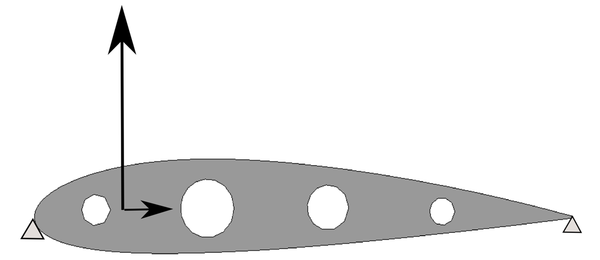
|

|
| Figure 52: Boundary conditions and discretization of the aerodynamic profile with an unstructured mesh. The partition of the domain by components is also shown. | |
As a starting point, micro-structure topologies with a circular hole that fulfills the desired fraction value are considered. Thus, the initial iteration corresponds indeed to a feasible iteration. In order to shed light on the alternate direction algorithm 5.3.3 of the component-based material design problem, we show, in Figure 53, the descent different directions in different columns. In the first column, we solve an equilibrium equation, which in optimization terms, leads to minimize the compliance respect to the stresses . The decrease on the cost due to the equilibrium is represented in blue on the cost function line. On the contrary, the decrease on the cost when selecting the optimal micro-structures (minimizing respect to ) is shown in red and it is represented on the second column of Figure 53.
Note that the algorithm converges extremely fast, almost one iteration of minimizing with respect to is needed to decrease the major part of the cost function. In this case, the optimal component-based material design solution provides an increasing of around a 16% of the stiffness with respect to the initial iteration by providing appropriate micro-structures on each component.
Bending beam We present the bending beam as the second Component-based material design example. The dimensions are 2 meter length 1 meter height, and plane stress conditions are assumed. The domain is discretized with a non-structured mesh with linear triangular element. The elastic properties of the basis material are: Young Modulus and Poisson ratio . In addition, the domain is regularly partitioned in 8 sub-domains (see Figure 54). The starting micro-structure topologies are taken as in the aerodynamic profile example. In Figure 54, intermediate and final iterations are also shown.
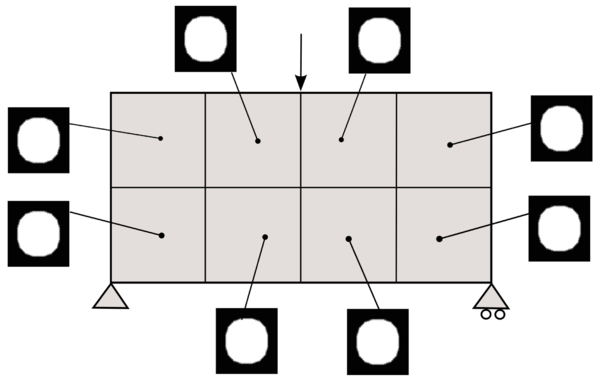
|

|
| (a) Iteration 1 | (b) Iteration 2 |
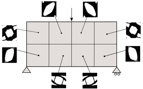
|
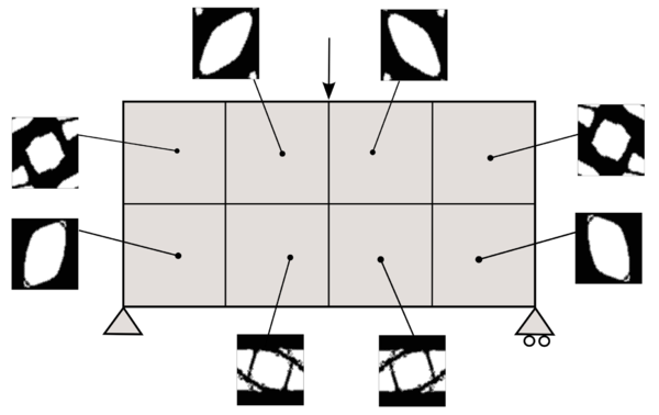
|
| Figure 54: Component-based material design problem applied to the bending beam example. Homogeneous material distribution is used in the first iteration and different micro-structures appear during the iteration process. The material is not designed Point-to-point, the same micro-structure is designed in all the sub-domain (fulfilling manufacturing constrains). | |
Note that, in this case, the Component-based material design algorithm converges in just four iterations.
5.3.5 Comparison between Point-to-point and Component-based material design problem
At this point, it is convenient to compare the Point-to-point and Component-based material design approaches. Certainly, both approaches tackle the same optimization problem with the difference that the former includes more number of design variables. According to equation (5.13), this fact should result into smaller values of the cost function. In Figure 55, the cost function for both approaches, in the case of the Bending beam example, is depicted. As expected, the Point-to-point material design approach achieves smaller values of the cost function.
In the case of Point-to-point material design approach, the compliance decreases around 35% while in the case of Component-based material design approach the compliance decreases around 18% In both cases the stopping criteria is taken as Note that, although a strong non linearity is faced, convergence is achieved in just few iterations. Additionally, it is worth stressing that, due to the Computational Vademecum, this two numerical examples have been solved in less than five minutes of computation with a standard PC (3.40GHz processor in a 64-bit architecture) in a Matlab environment.
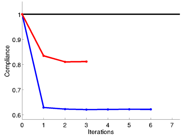
|
| Figure 55: Compliance comparison between Point-to-point (blue) and Component-based material design approach (red) for the Bending beam example. |
5.3.6 Consistency and efficiency
At this point, two different kind of approaches have been proposed to solve the problem: the Point-to-point material design approach that leads to optimal solutions without considering manufacturing conditions and the Component-based material design approach that considers manufacturing conditions at the cost of achieving sub-optimal solutions.
As mentioned in (5.11), the main idea of the Component-based material design approach lies on assuming homogeneous material distribution in each sub-domain. In principle, the sub-domain partition is a priory decided by the user depending on the particularities of the problem. However, it seems clear that, for a fixed domain, the number of variables of the optimization problem increases insofar as the number of sub-domains increases and, consequently, the objective function may decrease.
Therefore, the following question arises naturally: does a sequence of problems solved by the Component-based material design approach, in which the number of subdivisions increases, converge to the solution of the problem solved by the Point-to-point material design approach when the size of the sub-domains coincides with the size of the elements?. In other words, if the Component-based material design approach is applied to a problem with the size of the elements of the size of the sub-domain and its compliance is compared with the compliance obtained by the Point-to-point material design approach, do we obtain the same values? If this is the case, we say that the Component-based material design approach is a consistent approach.
Similarly, the second question arises as: if in the case of the study, the size of the sub-domain can be arbitrary decided, which size should be selected, and how will it influence on the cost function? This second question, later explained, is related with the efficiency concept.
Consistency Let's study a sequence of Component-based material design problems in which the number of sub-domains increases so that in the last cast each sub-domain coincides with the size of the elements. Then, we compare with the solution of the same problem solved by the Point-to-point material design approach.
To this end, we apply both methodologies to the Bending beam example. The domain is discretized with a regular coarse mesh of elements. We consider Finite Elements since they can be easily identified as a square sub-domain.
The sequence of problems with different sub-domains starts by considering the problem with only one sub-domain (homogeneous material distribution over all the domain). Then it is divided in and sub-domains. A full illustration of the sequence of problems used for the computations is shown in Figure 56. Regarding the boundary conditions, a concentrated force is applied in the middle top part of the domain and it is supported on the bottom corners. The dimension of the domain is .
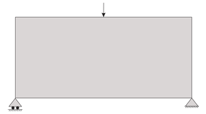
|
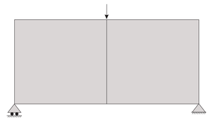
|
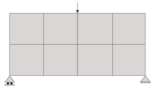
|
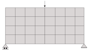
|
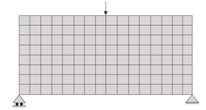
| |
| Figure 56: A sequence of problems, with different number of sub-domains, is represented. The aim is to study the convergence of the Component-based material design approach to the Point-to-point material design approach. | |
We depict in Figure 57 the values of the compliance.
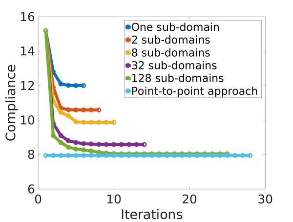
|
| Figure 57: Representation of the compliance values as a function of the number of iterations for the sequence of sub-problems shown in Figure 56. In sky-blue, the compliance for the Point-to-point material design approach is depicted. As expected, the Point-to-point material design solution behaves as a lower bound of the Component-based material design approach. |
We observe that in each case the minimums of the compliance decrease monotonically as the number of sub-domains increases. The increasing number of iterations required to reach the optimal solution should not be worrisome since in real applications, the number of sub-domains are expected to be small enough. Clearly, this behavior is a consequence of the increment of design variables produced by the increment of sub-domains.
The compliance of the Point-to-point material design approach is also included in Figure 57 as a reference. This solution can be interpreted a lower bound of the Component-based material design approach. This result illustrates the inequality constraint state in relation (5.13). Note that the compliance value obtained in this case of sub-domains, in which the elements and sub-domains coincides, is not equal to the value of the Point-to-point material design approach. The reason lies in the fact that, in the sub-domains, the four Gauss point of each element takes the same micro-structure while this is not the case in the Point-to-point material design approach. Hence, it achieves smaller values on the cost. In Figure 58, we can observe how the solution of the Point-to-point material design approach converges to the Component-based material design approach.
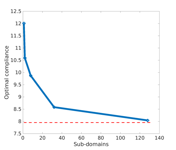
|
| Figure 58: Convergence of the Component-based material design approach to the Point-to-point material design approach. The compliance values are represented in blue for the sequence of problems using the Component-based material design approach shown in Figure 56. In red, the optimal value of the compliance obtained by the Point-to-point material design approach. Note the convergence of both approaches as the number of sub-domains converge to the number of elements. |
Efficiency To this end, we define the efficiency parameter as the normalized difference between the optimal solution obtained by the Point-to-point material design and the sub-optimal solution obtained by the Component-based material design with a fixed number of sub-domains, that is,
|
|
(5.16) |
According to the compliance inequalities stated in relation (5.13) holds, the efficiency parameter takes always positive values. In Figure 59, we depict the variation of the efficiency parameter with the number of sub-domains.
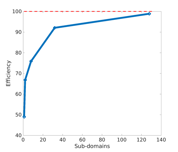
|
| Figure 59: Representation of the efficiency parameter as a function of the number of sub-domains. With just a small number of sub-domains, the solution is close the optimal (theoretical) solution. In view of this, Component-based material design allows obtaining manufacturing design at the cost of slightly reducing the stiffness of the structure. |
We first observe how the efficiency value increases when the number of sub-domains increases but this is at the cost of adding manufacturing limitations. Thus, the problem is governed by a trade-off between efficiency and manufacturing aspects. Figure 59, rather than determining the optimal number of sub-domain, shows the dependency between the efficiency and the number of sub-domains. The determination of the appropriate number of sub-domains falls on the interests and limitations of the user. In this sense, note that, in Figure 59, with only one sub-domain, i.e, by just deciding the optimal micro-structure used in the whole domain, we obtain almost a of efficiency. Note that the efficiency considerably increases with a slight increase of the number of sub-domains. This result shows that with just a small number of sub-domains, the solution is close to the optimal (theoretical) value.
5.4 Multi-scale topology optimization
At this point, instead of the standard macroscopic topology optimization problem, the Point-to-point material design approach (or the Component-based material design approach when considering manufacturing constraints) has been used to maximize the stiffness of the structure by considering the micro-structure topologies, instead of the macroscopic topology, as a design variable. However, one could maximize the stiffness of a structure by designing at the same time the macroscopic topology and the material design (microscopic topology in each macroscopic Gauss point). Hence, this problem is, hereafter, termed multi-scale topology optimization. Similarly, the multi-scale topology optimization may result into a Point-to-point or Component-based topological optimization.
5.4.1 Point-to-point multi-scale topology optimization
The main idea relies on solving a macro-structural optimization problem and, simultaneously, solve a Point-to-point material design problem in each iteration. This procedure is possible because of the efficient and the reduced time-consuming approach produced by the Computational Vademecum strategy. In mathematical terms, it can be understood as a generalization of the alternate direction algorithm by adding a new variable , which corresponds to the standard macro-structure topology optimization design variable. More specifically, due to the alternate direction algorithm, during the iterations, we can uncouple the macroscopic topology problem with the Point-to-point material design problem. For solving the latter, we naturally take profit of the algorithm proposed in section 5.2.3 .
Formulation Formally, the two-scale topology optimization problem can be presented in the following terms,
|
|
(5.17) |
The addition of the characteristic function extends the Point-to-point material design problem to the Point-to-point multi-scale topology optimization problem. Certainly, the comments described in the material design version remains true in the multi-scale version. Only, the additional difficulties of designing the macro-scale must be considered. Thus, the multi-scale topology optimization problem presents, even more evidently, strong non-linearities and high time-consuming computations. The number of design variables are of the order of the macroscopic Gauss-points times the microscopic Gauss-points for plus the order of macroscopic Gauss-points of and . Thus, in this problem, finding remedies to tackle the unaffordable computational cost of multi-scale topology optimization problem is mandatory.
Algorithm We propose a particular alternate direction algorithm in order to solve problem 5.17. More specifically, for each macroscopic topology optimization iteration, we solve a Point-to-point material design problem. Thus, the proposed alternate direction algorithm, alternates non-uniformly between the directions. In mathematical terms, we can re-formulate problem (5.17) as
|
|
(5.18) |
Thus, the problem is to find, for a fixed macroscopic topology , the solution of the inner problem (or loop) and then compute an iteration of the problem (or outer loop) in the Slerp algorithm. Therefore, the algorithm can be devised as an appropriate combination of the Slerp algorithm 1 and the Point-to-point material design algorithm 2. Full details are described in Algorithm 4.
|
Init: choose initial , , tol, , , and while do
|
|
Algorithm. 5 Point-to-point multi-scale topology optimization algorithm. It is devised as a shrewd combination of the Slerp and alternate directions algorithm. For each macroscopic topology optimization iteration of the Slerp algorithm, we solve a Point-to-point material design problem. |
It is worth stressing that this strategy is only possible because of the reduced time-consuming computation (due to the Computational Vademecum) needed for solving the Point-to-point material design problem.
5.4.2 Component-based multi-scale topology optimization
A further step entails manufacturing considerations. Emphasis is placed on the complexity of the problem. The addressed two-scale optimization problem presents not only strong non-linearities and large time-consuming computations, but also manufacturing constraints. To tackle it, we mimic the remedies proposed in the Component-based material design problem described in 5.11 for considering the manufacturing constraints. Thus, on the one hand, the material design problem is constrained to adopt, in each sub-domain, the same micro-structure. On the other hand, since the micro-structures are limited to the ones computed in the data-base, we solve a modified and sub-optimal problem.
Formulation More concretely, the Component-based multi-scale topology optimization can be formally formulated as
|
|
(5.19) |
where stands again for the number of sub-domains. Although the micro-structure topology is constant in each sub-domain, the optimization problem still considers a huge number of design variables. Note that, in the Component-based material design problem, the micro-structure is requested to be found in the Computational Vademecum.
Algorithm A natural way of extending the Component-based material design algorithm 3 to the Component-based multiscale topology optimization problem is to adapt Point-to-point multiscale topology optimization algorithm 4. In fact, the major difference lies on the way that the microscopic topologies are determined. Accordingly, these variables, instead of being solved from the Point-to-Point material design problem (5.3) with Algorithm 2, will be determined by solving the Component-based material design problem (5.11) with Algorithm 3. Note that again, this algorithm, alternates non-uniformly between directions. In mathematical terms, it consists of re-formulating problem (5.19) into
|
|
(5.20) |
Thus, similarly to the point-to-point version, the problem is, first, to solve and converge the inner problem (or loop) and then compute an iteration of the problem (or outer loop) in the Slerp algorithm. This final strategy is presented in Algorithm 5.
|
Init: choose initial , , tol, , , and while do
|
|
Algorithm. 6 Component-based multi-scale topology optimization algorithm. It is devised as a shrewd combination of the Slerp and alternate directions algorithm. For each macroscopic topology optimization iteration of the Slerp algorithm, we solve a Component-based material design problem. |
Again, the Computation Vademecum strategy allows this problem in affordable times.
5.4.3 Numerical results
In the following, two numerical examples are shown in order to asses the performance of the Point-to-point and Component-based multiscale topology optimization problems.
Cantilever beam As a first example, the standard Cantilever beam is considered. The domain is discretized with a structured mesh of elements. As shown in Figure 60, a concentrated force in the right side is applied whereas homogeneous Dirichlet boundary conditions (clamped) in the left side are imposed. The simultation starts with full material everywhere, the fraction volume is enforced to be and we take and . The stop criterion is taken as and .

|
| Figure 60: Schematic drawing of a Cantilever beam |
The aim is to compare all the proposed strategies and obtain an insight of its performance. In Figure 61, we evaluate the improvement of the compliance. First, in the left column, fixed micro-structure over all the domain (homogeneous) is considered, i.e., a standard macro-structure topology optimization problem is solved. Secondly, in the middle column, apart from the macro, the material design problem is point-to-point considered, i.e., the Point-to-point multi-scale topology optimization problem is solved. Finally, in the third column, we show the solution of the Component-based multi-scale topology optimization problem. To be fair in the comparison, in the macro-structure topology optimization case, we have considered a micro-structure with a feasible fraction volume .
Regarding the different algorithms, the left column shows how Algorithm 1 solves problem (3.35), the middle one, how Algorithm 4 solves problem (5.17), and the right one, how Algorithm 5 solves problem (5.19). In rows, we show some intermediate iterations and the final one.
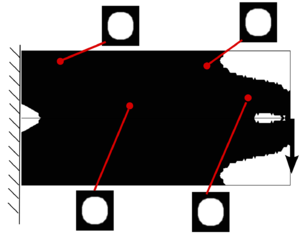
|
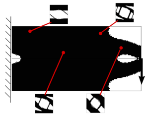
|
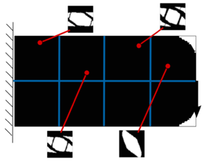
|
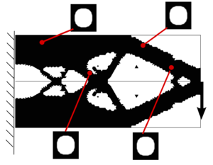
|
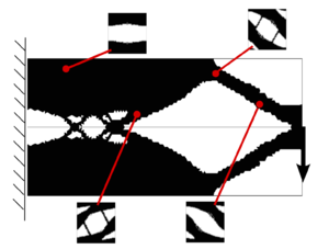
|
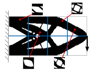
|
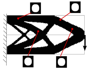
|
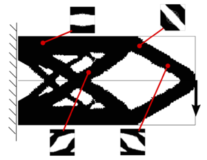
|
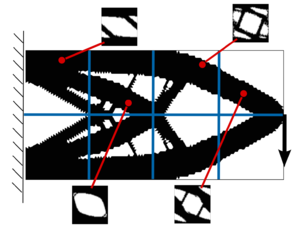
|
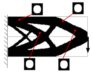
|
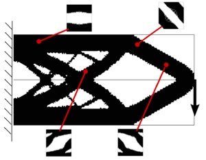
|
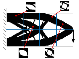
|
| Figure 61: Multi-scale topology optimization of the Cantilever beam. In the left column, the macro-scale topology optimization is solved. In the middle column, the Point-to-point multiscale topology optimization is solved. In the right column, the Component-based multiscale topology optimization is solved. Cost function values are shown in the last row. | |
Owing to the computational savings already mentioned in the section (no micro-structure computations are considered in the on-line process), we could solve all the problems in less than ten minutes of computation with a standard PC (3.40GHz processor in a 64-bit architecture) in a Matlab environment.
Interestingly, note that, on the one hand, we observe how the micro-structure topology design tries to mimic the macro-structure topology. On the other hand, as explained in Chapter 4, the microscopic topology clearly determines the macro-structure topology.
From the performance point of view, in Figure 62, we could see in black, the compliance when using the macro-structure topology optimization approach; in blue, the compliance when using the Point-to-point multi-scale topology optimization approach; and in red, the compliance when using the Component-based multi-scale topology optimization approach.
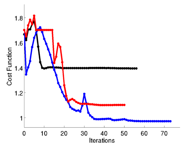
|
| Figure 62: Compliance values of the Cantilever beam example along the iterations. In black, the compliance when using the macro-structure topology optimization approach. In blue, the compliance when using the the Point-to-point multi-scale topology optimization approach. In red, the compliance when using the the Component-based multi-scale topology optimization approach. |
After decreasing a of the mass in the three cases allowing the possibility of designing the microscopic topology, the structure increases its stiffness in a in the Point-to-point multi-scale topology optimization problem and in a in in the Component-based multi-scale topology optimization problem with respect to the Macro-structure topology optimization solution.
Aerodynamic profile As a second example, the aerodynamic profile is considered. The Aerodynamic forces, computed by the strength vortex method [107], and the displacement boundary conditions are shown in Figure 63.
![Schematic drawing of an Airfoil geometry. A strength vortex method [107] has been used to compute the aerodynamic forces. The displacement conditions has been imposed to circumvent solid body motions.](/wd/images/thumb/f/f6/Draft_Samper_118254298-AirfoilForces.png/600px-Draft_Samper_118254298-AirfoilForces.png)
|
| Figure 63: Schematic drawing of an Airfoil geometry. A strength vortex method [107] has been used to compute the aerodynamic forces. The displacement conditions has been imposed to circumvent solid body motions. |
The aerodynamic profile is discretized with an unstructured mesh of finite elements (see Figure fig:AirfoilMesh-2).

|

|
The domain is partitioned (see Figure fig:AirfoilMesh-1) in the skin (red), the spar (blue) and the rib (gray). the The domain is started with full material, the final fraction volume is enforced to be and we take and . The stopping criteria is taken as and .
The results are shown following the same structure of the Cantilever Beam example. First, in the left column, fixed micro-structure over all the domain (homogeneous) is considered, i.e., a standard macro-structure topology optimization problem is solved. Secondly, in the middle column, apart from the macro, the material design problem is point-to-point considered, i.e., the Point-to-point multi-scale topology optimization problem is solved. Finally, in the third column, we show the solution of the Component-based multi-scale topology optimization problem. To be fair in the comparison, in the macro-structure topology optimization case, we have considered a micro-structure with a feasible fraction volume .
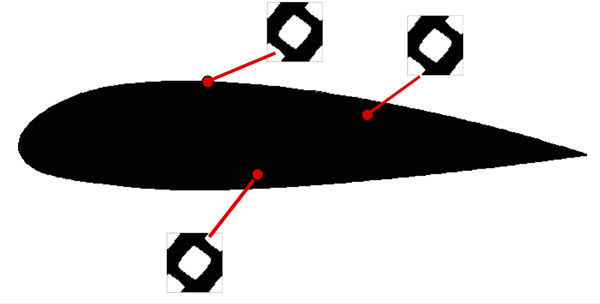
|

|

|
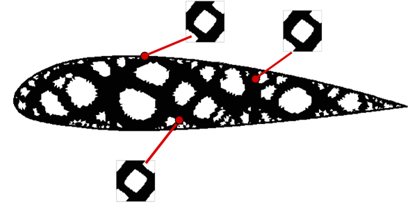
|
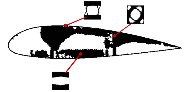
|
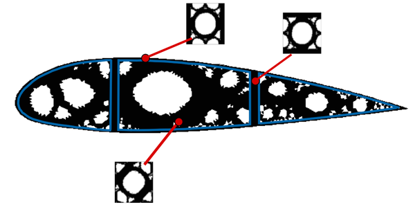
|
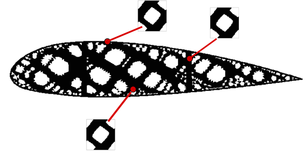
|
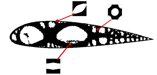
|
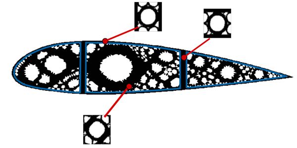
|

|
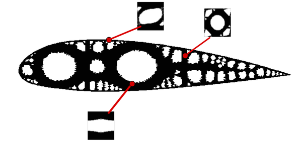
|
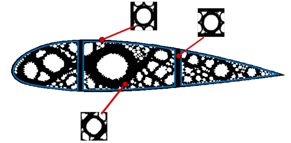
|
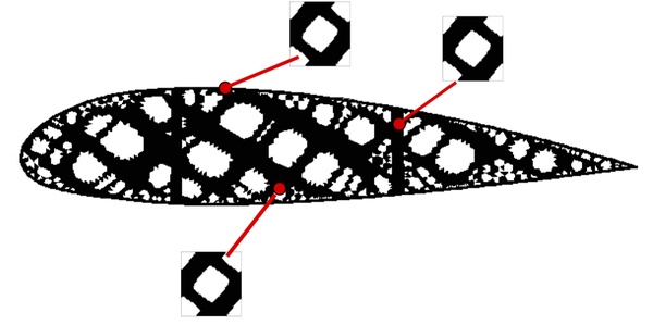
|
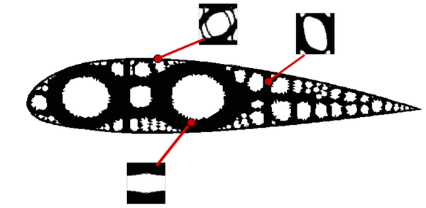
|
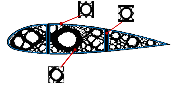
|
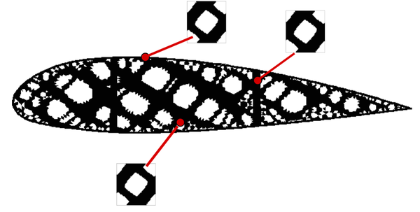
|
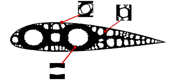
|
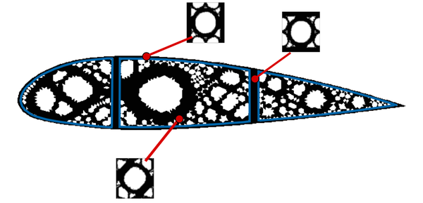
|
| Figure 64: Multi-scale topology optimization of the Aerodynamic profile example. In the left column, the is solved. In the middle column, the Point-to-point multiscale topology optimization is solved. In the right column, the Component-based multiscale topology optimization is solved. Cost function values are shown in the last row. | |
Owing to the computational savings already mentioned in the Computational Vademecum section (no micro-structure computations were required in the on-line process), we could solve all the problems in less than ten minutes of computation with a standard PC (3.40GHz processor in a 64-bit architecture) in a Matlab environment.
Again, it is noticeable how the micro-structure optimal topologies try to mimic the macro-structure optimal topology. This reveals the strong coupling between the microscopic and the macroscopic topologies.
Similarly to the Cantilever beam example, from the performance point of view, in Figure 65, we could see the different compliance values along the iterations. In black, the compliance when using the macro-structure topology optimization approach. In blue, the compliance when using the the Point-to-point multi-scale topology optimization approach. In red, the compliance when using the the Component-based multi-scale topology optimization approach.

|
| Figure 65: Compliance values of the Aerodynamic profile example along the iterations. In black, the compliance when using the macro-structure topology optimization approach. In blue, the compliance when using the the Point-to-point multi-scale topology optimization approach. In red, the compliance when using the the Component-based multi-scale topology optimization approach. |
After decreasing a of the mass in the three cases, when we allow the possibility of designing the microscopic topology, the structure increases its stiffness in a in the Point-to-point multi-scale topology optimization problem and in a in the Component-based multi-scale topology optimization problem. Certainly, the latter achieved smaller reduction of the cost. Nevertheless, it considers manufacturing constraints. These encouraging results evidence that considering the material design (Component-based) in the macroscopic topology optimization problem is highly recommended. Significant improvements () on the stiffness are obtained with non significant extra computational time (due to the Computational Vademecum).
5.5 Comments and limitations
In view of the multi-scale topology optimization results, a significant improvement of the stiffness is achieved with a strategy that entails no high time-consuming computations. However, it is convenient to comment some complementary aspects and some limitations of the problem.
5.5.1 Anisotropic topological derivative
In Chapter 4, the anisotropic topological derivative has been obtained and some numerical examples have confirmed its importance. However, when dealing with multi-scale topological optimization problems, the importance of the anisotropic topological derivative is even more evidenced. The optimal microscopic topology confers to the macro-structure (in each Gauss point) an anisotropic constitutive tensor. Certainly, although the isotropic topological derivative may be a reasonable descent direction, the anisotropic topological derivative permits solving the multi-scale topological optimization problem properly.
5.5.2 Saddle-point formulation
An important aspect to be highlighted is related with the statement of the problem. More specifically, in the problem, the stresses have been taken as the design variables for the equilibrium equation. However, alternatively, using the displacement or the strains would have been more natural. For more details of the two different formulation, we refer the reader to Chapter 1 of the reference book [1].
The problem expressed in terms of the displacement is as follows,
|
|
(5.21) |
On the contrary, the material design problem expressed in the complementary energy and depending on the dual variables is written as,
|
|
(5.22) |
Note that the primal formulation () consists on a saddle point problem whereas the dual formulation () consists on a classical minimization problem. A priori, the use of one or other formulation is arbitrary. This difference on the formulation could seem innocent, however the opposite is the case. Our numerical experience evidenced that the success depends on the approach.
The problem formulated in displacements has been tackled with no success. In the alternate direction algorithm, the iteration that should maximize the cost (changing the micro-structure topologies, i.e., changing variable ) advances overmuch leading the algorithm to diverge. The dual formulation seems to be better posed than the primal formulation.
As a remark, note that all this difference on the formulation is because of considering the compliance as a cost function. If, for instance, the volume is considered, no primal and dual formulation would appear (in the sense of minimizing the topology and displacements) and other algorithms (different from the alternate direction algorithm) should be considered.
This analysis of the primal and dual formulation is schematically shown in Figure 66.

|
| Figure 66: On the left, a minimization (min min) version of the material design problem. The stresses are regarded as design variables (dual formulation). On the right, a saddle point (max min) version of the material design problem is presented. The displacement are considered as the design variables (primal formulation). Since we have observed convergence difficulties in the saddle-point version, we have used the dual formulation in the material design problem. |
5.5.3 RVE geometry as a design variable
Having all the results of the material design and multiscale topology optimization problem in mind, it is convenient to comment some aspects about the RVE geometry. Up to now, the macroscopic stiffness of the structure has been maximized by means of the macroscopic topology and the microscopic topology . Regarding the latter, a square domain of the micro-structure have been used. However, other choices are possible. For instance, one could think on extending the space of design variables by introducing the geometry of the RVE. The possible geometries of the RVE are restricted to the ones that fulfill periodic boundary conditions (see section 2.33). Triangles, rectangles or hexagons are some examples.
In pursuing extreme materials, Sigmund in [1] uses, for example, parallelogram geometries. See also work [108] for more details.

|

|
|

|
| Figure 67: Different kind of micro-structures geometries that fulfill periodic boundary conditions. The possibility of using other kind of micro-structure geometries allow obtaining extreme materials with more optimal constitutive tensors. The Computational Vademecum conceives incorporating improved micro-structures with no needs of modifying the proposed methodology. | |
Note that, square, rectangular and hexagon geometries are indeed a particular case of the parallelogram. To be specific, one could parametrize the RVE by the inclination angle of the parallelogram and the aspect ratio of the sides. The square, the rectangle and the hexagon geometry can be recovered by considering specific values of these two variables. Thereby, the micro-structure design variables can be extended to the micro-structure topology jointly with inclination angle and the aspect ratio of the parallelogram. Thus, the possibility of using other geometries enhance the space of optimal solutions and the final optimal macro-structure may increase its stiffness.
Thus, the interest now deals with solving the material design problem not only respect to the topology but also respect to the geometry. In the case of the compliance, Allaire presents significant results in book [3]. It asserts that the optimal constitutive tensor is obtained after an homogenization process of a rank-2 laminate RVE.

|
![On the left, an optimal topology of a square RVE, on the right, a rank-2 laminate micro-structure. The Computational Vademecum can be improved by considering all kind of micro-structures (not only square RVEs). In the case of compliance, it can be seen that the optimal values are achieved when considering rank-2 laminates. [3].](/wd/images/a/a5/Draft_Samper_118254298-Rank2_Laminates.png)
|
| Figure 68: On the left, an optimal topology of a square RVE, on the right, a rank-2 laminate micro-structure. The Computational Vademecum can be improved by considering all kind of micro-structures (not only square RVEs). In the case of compliance, it can be seen that the optimal values are achieved when considering rank-2 laminates. [3]. | |
Referring to our work, the idea of increasing the design variable space or the possibility of using rank-2 laminates would complement the Computational Vademecum approach. Rather than being a drawback, it would enrich the pre-computed database. To this aim, it would be required to exchange the actual topologies and constitutive tensors (obtained with square RVEs) by the new optimal ones.
To our best knowledge, this fact is a clear advantage of the Computational Vademecum approach. The database can be improved if more optimal topologies are found or some manufacturing constraints must be added. However, the approach remains the same. Thus, the Computational Vademecum concept confers robustness and room for improvement to the approaches (material design and multi-scale topology optimization) proposed in this Chapter for increasing the stiffness of a structure.
5.5.4 Limitations
In view of the Point-to-point and Component-based multi-scale topology optimization results, an important improvement of the stiffness ( and ) has been achieved. In addition, the idea of generating the Computational Vademecum offers an appropiate and reduced time-consuming approach for solving the non-linear and large-scale optimization problem. However some inconveniences appear.
First, the Computational Vademecum is limited to a specific fraction volume. However, one could naturally think on extending the Computational Vademecum with an extra variable. Certainly, it would entail additional computations.
Second, in the void part of the domain, the microstructure topologies are also optimized. From the physical point of view, this options seems to be unreasonable. However, it is worth stressing that, strictly speaking, the void part behaves as a weak material and designing the micro-structure makes perfect sense. To avoid these computations, one may deactivate the void elements.
Finally, another clear limitation deals with extending the methodology to 3D problems. In this sense, the dimensions of the Computational Vademecum would significantly increase and the parametric space could no longer be represented by the unit sphere. However, one could replace the multi-scale topology optimization by a sub-optimal problem in which the optimal micro-structure topologies are sought in a reduced and representative sub-domain of the parametric domain. This study is left for future work.
5.6 Summary and conclusions
The present chapter addressed multi-scale topology optimization problems. Accounting for a two-scale computational homogenization scheme (), the optimization problem is governed by the influence of the design variables (defined at the micro-scale or, additionally, at the macro-scale) in the cost function (defined at the macro-scale).
To this aim, we first presented the Point-to-point material design problem as an alternative to the macroscopic topology optimization problem to maximize the stiffness of a structure. Likewise, in order to achieve manufacturing (and consequently sub-optimal) designs, a Component-based material design problem was also introduced.
The high complexity of the problem, which accounts for the few works devoted in the literature to this topic, was examined. A material catalog, termed Computational Vademecum in the present work, was built as an off-line computation to mitigate the unaffordable time-consuming computations of the problem. It allows circumventing the micro-structure topology-design effort in each sampling macroscopic point (in the Point-to-point material design case) or component (in the Component-based material design case) by selecting form the Computational Vademecum the pre-computed optimal microstructure topology. On the one hand, it is worth stressing that the Slerp algorithm jointly with the Mixed formulation presented in Chapter 2, manages to converge more than microscopic topology optimization problems. This success strengthens the use of the Slerp algorithm and exhibits its robustness. In addition, once the Computational Vademecum is available, it can be repeatedly consulted by any structure made of the same base material.
To deal with the strong non-linearity of the problem, an alternate direction algorithm was proposed. The results showed that a few number of iterations are needed to converge the problem. This finding suggests its use in multi-scale topology optimization problems. A key strength of both Point-to-point and Component-based material design approaches is that a considerable improvement of the structural stiffness ( and respectively) was achieved.
Additionally, we examined the convergence of the Component-based material design approach to the Point-to-point material design approach, which results in a consistent relation between both approaches. Furthermore, the presented efficiency parameter helped on determining the appropriate number of components, which is governed by the trade-off between the stiffness of the structure and the manufacturability constraints.
A second and even more stimulating part of the study consists in using complementary (instead of alternatively) the Point-to-Point or Component-based multiscale topology optimization jointly with the macroscopic topology optimization problem. Since the optimal microscopic topologies collected in the Computational Vademecum confers anisotropic constitutive tensors, the anisotropic macroscopic topology optimization problem accounts for the use of the anisotropic topological derivative, obtained in Chapter 4.
The Point-to-Point and Component-based multiscale topology optimization provided an additional (around and ) increase of the stiffness over the already increase obtained by the macroscopic topology design. In addition, due to the Computational Vademecum concept, all the examples were solved in less than ten minutes of computation with a standard PC (3.40GHz processor in a 64-bit architecture) in a Matlab environment. When examining the results, a strong coupling between the macro and micro scale, not only from the mechanical point of view but also from the topological point of view, were observed. Yet, the numerical examples confirmed the success of the dual formulation ( in stresses) rather than the primal formulation (in strains).
Nowadays, the Computational Vademecum concept could be straightforward adapted to industrial problems. The current RVEs would be replaced by a standard composite material and the microstructure design variables by the orientation of fibers and number of plies.
Regarding the short future, if new optimization tools appear for obtaining improved microscopic topologies, the Computational Vademecum can be enhanced replacing the current microstructure topologies by the improved ones. The micro-structures would be replaced, but the Computational Vademecum would remain useful. Certainly, additional research is needed to extend the methodology to 3D problems.
6 Conclusions
6.1 Achievements
This study adresses multi-scale topology optimization problems. As reported in the literature, the problem evidences a large complexity and high computational cost. The challenge was to devise appropiate algorithms and techniques with the capability of solving the problem in a robust and efficient fashion. This was achieved by enhancing the current topological derivative algorithms, by obtaining a closed-form of the anisotropic topological derivative and by proposing algorithms and shrewd reduction techniques for dealing with multi-scale topology optimization problems.
In Chapter 3, we could thoroughly establish the foundations of using topological derivative in topology optimization problems. The numerical instabilities presented by the Slerp algorithm has been treated by different authors using re-meshing techniques. We have managed to avoid it by proposing a Mixed formulation approach to deal with the interface elements. The Slerp algorithm has evidenced a considerable improvement. On the one hand, spurious local minima have vanished when determining the line-search parameter. On the other hand, the Slerp algorithm is now able to converge (with no need of re-meshing techniques) leading to significant computational savings.
In Chapter 4, we have obtained a closed-form of the topological derivative for anisotropic materials. A deep understanding of the transform and the complex variable has led to solve analytically the exterior problem of a infinite anisotropic domain with an anisotropic circle inclusion. Complementary, the exterior problem, in the case of isotropic materials, has been also solved analytically through the Airy function. Full details are collected in Appendices 7 and 8. We have checked that the expression of the anisotropic topological derivative expression coincides with the the isotropic version when considering isotropic materials. Additionally, the anisotropic topological derivative expression have been validated through a set of convergent numerical experiments. The obtained expression has opened the possibility of solving the topology optimization problem when dealing with anisotropic materials. The achieved optimal topologies have evidenced the strong dependency of the optimal topology with the anisotropic material response.
In Chapter 5, we have tackled the multi-scale topology optimization problem. The strong non-linearities presented by the problem have been mitigated due to the use of an alternate directions algorithm. Furthermore, the use of a Computation Vademecum, which has been computed as a previous step (off-line), has saved much of the computational cost of solving the microscopic topology optimization problem in each macroscopic Gauss point. In addition, the huge () optimal microscopic topologies collected in the Computational Vademecum evidenced the robustness of the Slerp Algorithm when using the Mixed-formulation approach. A significant improvement, increase of around and of the structural stiffness, has been achieved considering the Point-to-Point and the Component-based material design approach respectively. Additionally, when considering both the macroscopic and microscopic topologies, on top of the increased stiffness already obtained by optimizing the macro-scale, an extra increased stiffness around or is obtained by optimizing the micro-scale, depending if the Point-to-Point or the Component-based multiscale topology optimization approach is used. The obtained results have evidenced that, with the methodology proposed in this work, a two-scale topology optimization problem can be solved in less than ten minutes of computation with a standard PC (3.40GHz processor in a 64-bit architecture) in a Matlab environment.
6.2 Concluding remarks
- The topological derivative evaluates the sensitivity of a cost function when inserting an inclusion in the domain. In view of the results, the topological derivative, in conjunction with the Slerp algorithm, results in a powerful tool for solving topology optimization problems. On top of that, the Mixed formulation has contributed in endowing robustness and computational savings to the algorithm; no re-meshing techniques are now necessary. We believe that this approach is an appropiate strategy to solve topology optimization problems since no heuristic parameters are involved, no large gray regions appear and no high time-consuming computations must be considered.
- The anisotropic topological derivative has opened the possibility of extending the method to anisotropic materials. We believe that the burdensome computation of the anisotropic topological derivative is accounted for the high use of the anisotropic materials in industrial applications. In addition, when addressing multiscale topology optimization problems, the optimization of the macroscopic topology makes use of the anisotropic topological derivative, since the computational homogenization of microscopic topologies infers anisotropic response to the macro-scale.
- We consider that the optimization problems, in which the design variables are of different nature but can be clearly distinguished or grouped, lend themselves to be solved by means of the alternate direction algorithm.
- In the case of multiscale topology optimization, we can naturally distinguish between three groups: the stresses, the macroscopic topology and the microscopic topologies. Each group of variables can be updated (with an appropiate algorithm) by freezing the other groups of variables. In this work, the three algorithms are: the equilibrium equation for the stresses and the Slerp algorithm for the both macroscopic and microscopic topologies. Although the alternate direction converges linearly, in our case, only few iterations have been needed to solve the problem.
- As a main drawback, the alternate direction algorithm can become inappropriate when significant computational costs are needed to solve one group of variables. In our case, the bottle-neck of the problem consists in the optimization of the microscopic topologies. We have circumvent this difficulty by first obtaining and collecting in the Computational Vademecum the optimal microstructure topologies, and then by selecting them during the coupled optimization problem. This results in insignificant computations when optimizing the microscopic topologies. We believe that these approach can be straightforwardly tailored to other complex and coupled optimization problems, specially when multiscale techniques are involved.
- In conclusion, all the algorithms and methods proposed throughout this study constitute a initial seedbed of the multi-scale topology optimization techniques. The results of this work clearly show how the stiffness of a structure can be improved by means of material design. Although designing the microscopic topology is not standard nowadays in industrial applications, the promising new additive manufacturing techniques, like 3D printing, seem to be able to make true in the short future.
6.3 Future work
Certainly, the framework built in this study represents a foundation for future developments in multi-scale topology optimization problems. Some of them have been suggest throughout the dissertation. They are summerized in the following points:
- The Slerp algorithm presents a bothersome behavior when dealing with cost functions that tends to zero in the optimal. In this case, it results in that the topological derivative tends also to zero. Since the aim of the algorithm is to preserve parallelism between the level-set and the topological derivative (zero in this case), the convergence is no longer achieved. Undoubtedly, future developments should consider tailoring the algorithm to this kind of problems.
- Regarding the alternate direction algorithm, excellent results have been achieved when compliance and volume are considered as the cost function and the constraint respectively. A more natural approach would be minimizing the volume and ensure that the stress state remains under a certain value. However, in this case, the alternate direction algorithm can not be straightforwardly used. New strategies for solving the multiscale topology optimization problem when no considering the compliance should be devised in future work.
- Regarding 3D problems, two kind of difficulties must be studied. On the one hand, the computation of the anisotropic topological derivative has been restricted to 2D problems. However, the 3D anisotropic topological derivative expression can be considered as one of the most challenges of the topic in the short future.
- On the other hand, new techniques must be devised to extend the parametric domain of the Computational Vademecum since, up to now, it is parametrized by only two design variables. Being capable to encompass 3D problems and extending the Computational Vademecum through the Poisson ratio and the volume fraction would represent a major breakthrough. For this purpose, as a future work, we believe convenient resorting to two of the most emerging model reduction techniques: the proper orthogonal decomposition (POD) or the proper generalized decomposition (PGD).
A Analytical solution of the isotropic exterior problem
In this Appendix, we aim at solving analytically the exterior problem in order to compute the final expression of the topological derivative.
It consists in solving a two dimensional problem in plane stress for an isotropic infinite domain (hereafter referred matrix) with a unitary centered circular inclusion inserted of another isotropic material. Two kind of boundary conditions are considered; firstly, at infinity the stresses are imposed to be zero; and secondly, due to the Eshelby theorem a constant behavior of the stresses is imposed in the inclusion. In addition, the transmission conditions (in stresses and displacements) across the interface of the inclusion and the matrix are also considered. All that conditions are necessary for solving the free constants appearing in the problem.
The process of solving the exterior problem and of getting the final expression for the polarization tensor, is organized as follows. First, the equilibrium equation and the Beltrami-Michell compatibility equations are introduced using a Cartesian coordinate system. Then, since a circular inclusion is considered in the problem, both the equilibrium and the Beltrami-Michell compatibility equations are expressed in polar coordinates. The Airy function is proposed as the only unknown to be found in the problem such that, on the one hand, it satisfies automatically the equilibrium equation, and on the other hand, its expression can be determined by solving the Beltrami-Michell compatibility equation, which in terms of the Airy function becomes a biharmonic equation. Next, the boundary and transmission conditions are imposed to find the free parameters appearing in the Airy function for both the matrix and the inclusion. Finally, we express the stresses on the inclusion in terms of the stresses tensor that appear in the normal stress jump across the interface of the inclusion and the matrix. This last relation represents the main ingredient for computing the topological derivative.
Notice that, on the exterior problem (4.19), the stresses on the inclusion are denoted by and the displacements by . For convenience, we change notation as follows
|
|
A.1 Equilibrium and Beltrami-Michell equations
The general equilibrium equation is normally expressed as
|
|
where and represents the body forces an the inertial terms. Neglecting both terms, and using a Cartesian coordinate system, the equilibrium equation is written as
|
|
(A.1) |
in which we assume a 2D plane stress behavior. Then, the Airy function is defined by enforcing the second derivatives to fulfill
|
|
(A.2) |
Note that with this definition the equilibrium equation (A.1) is automatically satisfied. The equilibrium equation is necessary but not sufficient to be a solution of an elasticity problem. In addition, the compatibility conditions must be satisfied, which in terms of stresses (commonly called Beltrami-Michell compatibility conditions) with considering no body forces takes the following form
|
|
(A.3) |
Thus, the laplacian of the trace of the stress tensor must be zero. Clearly, in Cartesian coordinates, the laplacian is denoted as
|
|
Inserting the stresses of equations (A.2) in terms of the Airy function in the Beltrami-Michel compatibility equation (A.3), we obtain
|
|
which stands for the biharmonic equation for the Airy function. Commonly, it is also expressed as
|
|
However, since we deal with a circular inclusion, it is more appropiate to reformulate the problem in polar coordinates. We can now proceed analogously to the equilibrium equations which in this case are writing in the following form
|
|
(A.4) |
Similarly, the Airy function is defined fulfilling
|
|
(A.5) |
Note that, again, with these definitions, the equilibrium equation (A.4) is automatically satisfied.
Considering the independence of the first invariant on the system of coordinates, that is , according to equation (A.3), we have
|
|
(A.6) |
Likewise, the laplacian in polar coordinates takes the following form,
|
|
Substituting the stresses in terms of the Airy function from equation (A.5) into the Beltrami-Michel equation (A.6), we obtain the biharmonic equation for the Airy function in polar coordinates, that is,
|
|
(A.7) |
For simplicity, the biharmonic equation is also commonly expressed more schematically in the following form
|
|
A.2 Boundary and transmission conditions
For the solution of the biharmonic equation, we need to define the boundary conditions that must be satisfied. It is worth mentioning that since we consider two bodies (inclusion and matrix), two Airy function appears as the unknowns of the problem, one for each body.
Regarding the matrix, in the way that the exterior problem is defined, we impose that at infinity the stresses cancel, this is,
|
|
Note that all the variables (Airy function , the stresses and the strains ) are hereafter denoted by a super-index in the case of the matrix and in the case of the inclusion
Regarding the boundary conditions for the inclusion, we impose the Eshelby theorem [109,110,111], which asserts that the strain fields inside the inclusion are constant if the loading at infinity is constant (zero in this case). For further information of the Eshelby theorem, the reader is referred to works [112,113]. Thus, for the case of elastic materials, the constant value of the strain field brings constant value of the stress field, i.e.,
|
|
(A.8) |
Note that the dependency on is due to the dependency of the basis (polar) on which it is expressed, but not on the values of the tensor. If it is expressed in the principal coordinates no dependency on appears.
This dependency on is clearly seen when we impose the jump on traction across the boundary of the inclusion. Thus, once the boundary conditions are imposed in both solids, the transmission conditions across the interface of the inclusion and the matrix must be satisfied. Regarding the stresses, the exterior problem is defined such that the jump of the traction across the interface must be equal to the normal component of the given stress tensor , this is
|
|
(A.9) |
Thus, the stresses will be discontinuous across the interface. Although the exterior problem is solved in polar coordinates, the data and the solution must be provided into Cartesian coordinates. Thus, we try to re-express the tensor in polar coordinates in terms of its Cartesian counterpart. Pre and post-multiplying by the standard rotation matrix, we obtain
|
|
Accordingly, if we proceed to express the relation in vector notation as
|
|
and after applying the trigonometric identities and , we shall write the above expression as
|
|
which in a matrix-vector representation takes the following form
|
|
(A.10) |
Thus, both the first and the last equation of the above expression are going to be considered in the transmission conditions (A.9). Note that although the tensor is constant a dependency on appears due to its representation on the polar basis of the tensor. This is analogous to the inclusion stresses dependency that appear in the Eshelby conditions (A.8). The dependency on the angle appears due to its representation on the polar basis.
Regarding the transmission conditions on displacements, we must ensure, in polar coordinates, that the jump across the boundary of the inclusion of the component of the strains must be zero (see [114] for further information), i.e.,
|
|
(A.11) |
The biharmonic equation jointly with all these conditions are the necessary ingredients for solving the exterior problem.
A.3 Resolution of the biharmonic equation
Since we have to satisfy the transmission conditions and the tensor is expressed in equation (A.10) as a combination of , and , the Airy function is proposed at least depending on that terms. More specifically, that is
|
|
Introducing the above expression in the biharmonic equation (A.7), we obtain
|
|
Considering the biharmonic operator, the following equations can be written
|
|
We now proceed to study and solve (up to constant parameters) each term of the Airy function and then we sum them up.
Regarding the term , it must satisfy
|
|
and after applying the change of variable , the above equation becomes the following linear one
|
|
(A.12) |
Since it has linear behavior, we can solve it through the characteristic equation
|
|
whose roots (both doubles) are and . Thus the solution of equation (A.12) reads as
|
|
and after undoing the change of variable, we obtain
|
|
which can be expressible in a vector form as
|
|
We proceed similarly for the function . The compatibility equation is written as
|
|
After applying the same change of variable and solving the characteristic equation, we obtain that the term is of the form
|
|
Undoing again the change of variable, we end up with the expression for as
|
|
which can be written in a vector form as
|
|
Since has to solve the same equation than , it can be written in the same terms, that is
|
|
Thus, the Airy function is compactly expressible as
|
|
(A.13) |
The free parameters are collected in the vectors , and and are going to be determined after applying the boundary and transmission conditions.
A.4 Resolution of the free parameters
Once we have the expression of the Airy function, we move to compute the field. According to relations (A.5) and considering the expression (A.13), we obtain
|
|
Note that each term of the matrix stands for a scalar product between the , , and some derivatives of , and . Let us define the following relation by
|
|
(A.14) |
in which each term , , , , , ,, and are computed as follows
|
|
|
|
|
|
|
|
|
|
A.4.1 Boundary conditions in the matrix
For determining the free parameters, we first apply on the matrix the condition (A.8) of zero stress at infinity which leads to cancel the following constants
|
|
Since the last term of and is canceled there is no reason of keeping the constant hence
|
|
Consequently, the vectors , and become
|
|
and similarly the vectors becomes
|
|
|
|
Substituting all these reduced expression into equation (A.14), we are ready to compute the term that appears in the transmission condition just imposing as follows
|
|
(A.15) |
A.4.2 Boundary conditions in the inclusion
Regarding the conditions on the inclusion, we have to impose a constant value of the stressed as it is detailed in (A.8). Thus, all the constants that multiply terms that depend on variable are canceled, that is
|
|
And similarly, since is arbitrary and it does not appear on the stress, there is no reasons to keep it. Hence,
|
|
Consequently, the vector , and become
|
|
and the vector are reduced to the following expression
|
|
|
|
In order to apply the transmission condition, substituting the above reduced expression in the stress field equation (A.14), we obtain the constant stress field in the inclusion as
|
|
(A.16) |
Note that since the stresses are constant in the inclusion, the above expression stands also for the stresses on the interface.
It is worth mentioning that if we write the stresses into the Cartesian components analogously to expression (A.10) as
|
|
and we identify all the terms of both matrices, we can relate the Cartesian components of the stresses with the constants , and as
|
|
which in matrix notation is written as
|
|
(A.17) |
That last relation will be useful to find the final expression for the topological derivative. With all these boundary conditions imposed, we end up with 8 unknowns , , , ,,, and that are going to be determined after imposing the transmission conditions.
A.4.3 Stress transmission condition
We apply the transmission condition in stresses across the interface. The first equation of (A.9) imposes continuity on the radial component of the stress as
|
|
Considering the matrix representation (A.10) of the stress and comparing it with the difference with the matrix representation of the stresses on the matrix (A.15) and the inclusion (A.16), we can identify the , and terms and write the following equations
|
|
(A.18) |
Similarly, according to (A.9), the continuity of the shear component is imposed as
|
|
Considering again the matrix representation of , and and identifying the , and terms, we can write the second group of equations as
|
|
(A.19) |
A.4.4 Strain transmission condition
The last condition to impose is the strain transmission condition (A.11). Since we assume plane stress and isotropic material behavior, the strain can be related with the stresses for both the matrix and the inclusion through the following inverse constitutive relation
|
|
|
|
where , , and represents the Young modulus and Poisson ratio for the matrix and the inclusion. Inserting the above relation in the transmission condition (A.11) and considering equations (A.15) and (A.16), we can write the last group of equations as
|
|
(A.20) |
A.5 System of equations for the free parameters
Adding and rearranging all the group of equations, we can split them in three groups as
|
|
|
|
|
|
The matrices of the three system of equations are invertible, thus, all the constants can be uniquely determined.
Regarding the , and , we provide its values in a matrix form as
|
|
where the matrix has been introduced and the adimensional constants and take the following values
|
|
Thus, according to expression (A.17), we can write the stresses on the inclusion in terms of the stresses as
|
|
where we have introduced the matrix . Thus, after solving the exterior problem through the Airy function, the boundary and transmission conditions, we have obtained a linear expression that relates the stresses in the inclusion with the stresses as
|
|
The appendix closes with this last relation since by substituting A in (4.34), we have obtained the polarization tensor which uniquely define the topological derivative.
B Analytical solution of the anisotropic exterior problem
In this appendix, we solve the exterior problem for an anisotropic infinite domain with a circular inclusion of an other anisotropic material. Henceforth, we call matrix to the material of the infinite domain and inclusion to the other one. The boundary and transmission conditions are equivalent to the isotropic case. This is to say, we impose in the matrix zero stress value at infinity and constant stresses to the inclusion due to Eshelby theorem. Regarding the transmission condition, we enforce continuity equilibrium on the normal direction of the stresses and continuity to the displacements.
The solving process is organized as follows. First, similarly to the isotropic case, we define a potential that satisfies automatically the equilibrium equation. However, we use Cartesian coordinates and a complex potential whereas in the isotropic case, the potential is defined as a real function and polar coordinates are considered. Then, we enforce that the potential satisfies the compatibility equation in stresses, but now it does not result to the Beltrami-Michel equations, since anisotropic materials are considered. After integrating the compatibility equation and defining an intermediate potential, we provide some results of complex variables and we impose the transmission conditions for the stresses and displacements. We also provide a justification for the anstatz used and we determine in a matrix form the system of equation needed for solving the problem. Finally, since the problem is too complex to be solved directly by a symbolic software, we provide some properties which makes the problem more compact and solvable by such symbolic software.
The main ideas and part of the notation have been extracted form the classical book [47].
Notice that, on the exterior problem (4.19), the stresses on the inclusion are denoted by and the displacements by . For convenience, we change notation as follows
|
|
B.1 Equilibrium equation and compatibility conditions for anisotropic materials
As mentioned in the isotropic Appendix 7, the equilibrium equation in Cartesian coordinates reads as
|
|
(B.1) |
where the body forces have been neglected. We define the potential (stress function in book [47] and homologous to the Airy function) as,
|
|
(B.2) |
Note that the potential satisfies automatically the equilibrium equation (B.1). The strain compatibility conditions in plane stress reads as
|
|
(B.3) |
Assuming elastic behavior the anisotropic constitutive law in its inverse form is written as
|
|
(B.4) |
where with are the components of the constitutive tensor (in matrix notation). Inserting the relation (B.2) into the constitutive law (B.4), and the constitutive law into the compatibility condition (B.3), we obtain
|
|
Following the integration procedure of the book [47] (Page 29), the potential can be written as
|
|
where denotes the real part and and define a new coordinate system
|
|
in which the parameters with , are the solutions of the characteristic equation
|
|
(B.5) |
We define the anisotropic potential and as the derivative of the potential , this is,
|
|
(B.6) |
Substituting the above definition into equations (B.2), the stress tensor is expressed as follows
|
|
(B.7) |
Regarding the displacement, in the small strain context, the strains can be written in terms of the displacement as
|
|
(B.8) |
Integrating the above expression and taking into account the constitutive law (B.4), it is easy to see (detailed in book [47]) that the displacements may be written as
|
|
(B.9) |
where characterize a rotation and the complex numbers and are defined as
|
|
(B.10) |
8.2 Special case of a infinite plate with an inclusion
The idea is now to apply the above definitions to the concerning problem, i.e., the case of an infinite plate with an inclusion.
Regarding the stresses, on the one hand, the stresses appearing in the matrix, hereafter referred , are derived from the anisotropic potential detailed in equation (B.7). On the other hand, according to the Eshelby theorem [109,110,111], the stresses in the inclusion are constant. Thus,
|
|
Regarding the displacements in the inclusion, since we deal with constant strains (Eshleby theorem), the equation (B.8) becomes
|
|
Integrating the first two terms as follows
|
|
and inserting the above expressions in the third term, we obtain
|
|
and integrating again respect to the Cartesian coordinates, the function and read as
|
|
Redefining the constant by , and neglecting the rigid body displacement and , the displacement on the inclusion in a matrix form is expressed as
|
|
(B.11) |
Regarding the displacement on the matrix, according to equation (B.9), they are derived from the anisotropic potentials and as
|
|
(B.12) |
Rearranging the above expression in a matrix form, we finally obtain
|
|
B.3 Coordinates in the inclusion
Before imposing the transmission condition, let us study the values of the coordinates on the inclusion. Since we assume that an elliptic inclusion (circular in this case) is inserted, the coordinates can be written in elliptic coordinates as
|
|
or in matrix form as
|
|
(B.13) |
where the sub-index denotes the value on the elliptic inclusion. The complex variable in the elliptic inclusion is expressed as
|
|
and its square value as
|
|
Thus, applying simple trigonometric algebra, we can compute the following equation
|
|
Finally, defining the complex variable on the inclusion is reduced to
|
|
we end up with the simplified following expression
|
|
Thus, both coordinates and can be written in terms of the complex variables as
|
|
(B.14) |
B.4 Transmission conditions
We proceed now to impose the transmission conditions through the interface of the inclusion and the matrix. Both conditions in stresses and in displacements will provide the necessary conditions to solve the constants of the problem.
B.4.1 Transmission conditions in stresses
Since we want to solve the exterior problem stated in equation (4.39), the difference of the stresses between the inclusion and the matrix in the normal direction must be the traction caused by the given stresses , this is
|
|
Note that the stresses on the matrix are denoted by the sub-index . By contrast, since the stresses on the inclusion are constant, they are no longer needed to be denoted by sub-index . Re-expressing it in matrix notation, we obtain
|
|
(B.15) |
Defining the vector position in terms of a parametric coordinate in the inclusion as
|
|
the tangent and normal read as
|
|
Now, owing to the above expression and equation (B.2), we proceed to express a general stresses tensor projected in the normal direction as
|
|
where we have used the property of exchanging the derivatives. Using this last expression in equation (B.15) for each stress tensor and , we can re-write the transmission condition as
|
|
where , and represents the matrix potential, the inclusion potential and the potential of the given stresses . Integrating the above expression over all the inclusion, the following equality holds
|
|
(B.16) |
Note that in the last step we have rearranged the order of the equations. Since the given stresses and the stresses in the inclusion are constant, integrating expression (B.2), the potentials and can be written as
|
|
Thus, the right hand side of equation (B.16) can be computed as
|
|
(B.17) |
Regarding the left hand side, expression (B.6) yields
|
|
(B.18) |
Inserting these two last equation (B.17) and (B.18) in (B.16), we finally obtain the transmission condition in terms of the anisotropic potentials and as
|
|
(B.19) |
Note that using the relation (B.14), the transmission condition can be computed also by the following equation
|
|
(B.20) |
B.4.2 Transmission conditions in displacements
Similarly, we impose the transmission condition in displacements stated in equation (4.39). The displacement field must be continuous on the interface, i.e,
|
|
According to the expression obtained in equation (B.11) and (B.12) for the displacement in the inclusion and in the matrix, it is convenient to rewrite the transmission condition in displacements as
|
|
Defining a global rotation as , we end up with the following expression of the transmission condition in displacements
|
|
(B.21) |
Note that if we consider the relation (B.14), the above equation reads as
|
|
(B.22) |
B.5 Proposing the ansatz
According to the reference book [47] (Page ), the ansatz for the anisotropic potentials and for an infinite plate with an elliptic inclusion an constant stresses at infinity (zero in our case) is of the form
|
|
where , , ... and , , ... are a priori complex constants to be determined. However, taking into account the expression obtained in the transmission conditions (B.20) and (B.22), they must take the following values
|
|
where and are rewritten as and Thus, the anisotropic potentials read as
|
|
In order to apply the transmission conditions, the anisotropic potentials in the inclusion are obtained as
|
|
and splitting the complex numbers and in its real (,) and imaginary part (,), we obtain
|
|
(B.23) |
B.6 Compact form for the transmission conditions
We proceed now to rewrite the transmission condition in compact form for both the stresses and displacements.
B.6.1 Compact form for the transmission conditions in stresses
According to the matrix expression (B.23) of the anisotropic potentials and the relation (B.13), the transmission condition in stresses (B.19) becomes
|
|
Since it must be satisfied for all , we shall rewrite the above expression as
|
|
where we have organized the unknowns and in the vector . Note that it helps us to define the matrices ,, and the vectors and . Thus, defining the matrix as
|
|
the left and right hand side of the transmission conditions for the stresses are reduced to
|
|
(B.24) |
B.6.2 Compact form for the transmission conditions in displacements
Similarly, according to the matrix expression (B.23) of the anisotropic potentials and the relation (B.13), the transmission condition in displacements (B.21) becomes
|
|
Since it must be satisfied for all , the terms of and disappear. We shall write the left hand side of the above expression as
|
|
where again we have organized the unknowns and in the vector and we have defined the matrix Regarding the right hand side, we rearrange it as follows
|
|
where the matrix has been defined. Taking into account the constitutive law (B.4), we can express the vector of the strains in the inclusion as
|
|
where we have introduced the definitions of the matrices and . Thus, in compact form we can write
|
|
(B.25) |
Similarly, the rotation term is expressed as
|
|
(B.26) |
where the matrix has also been defined. Thus, defining the matrix as
|
|
the left and right hand side of the displacements transmission conditions become
|
|
(B.27) |
Note that the right hand side, according to (B.25) and (B.26), can be also expressed as
|
|
(B.28) |
B.7 System of equations for solving the exterior problem
At this point, we proceed to write the full system of equations. By definition, the left and right hand side must be equivalent, i.e.,
|
|
Considering expressions (B.27), (B.28) and (B.24), the necessary system of equations are written as
|
|
Note that although and are the unknowns of the system of equation, we are only interested in the relation between with . To this end, we isolate variable from the first equation and we inserted in the second one, thus, we obtain
|
|
Grouping and terms, the above expression reads as
|
|
(B.29) |
where and have been defined. Thus, the unknowns can be found in terms of by solving the following equation
|
|
Since we are only interested in the stresses in the inclusion in terms of the given stresses , we pre and post multiply by the matrix as follows
|
|
Finally, we can identify the matrix as the matrix that pre multiply the given stresses , i.e.,
|
|
(B.30) |
Thus, the obtained linear relation
|
|
provide us the necessary result to compute the topological derivative.
B.8 Practical implementation for computing the matrixB.8 Practical implementation for computing the
A
{\displaystyle A}
matrix
Although the matrix is well defined and might be obtained only by using the corresponding definitions, our experience shows us that, in practice, it is computational unaffordable when using symbolic softwares to compute its explicit expression. We have to make use of some algebraic properties of the complex numbers.
Basically, the critical operation lies on the term which appears in and . By definition it is written as
|
|
On the one hand, we will prove that the term satisfies
|
|
(B.31) |
and, on the other hand, we will prove that the following relation holds
|
|
(B.32) |
where operator takes the imaginary part and is further defined. With these properties at hand, the term can be written as
|
|
(B.33) |
where the complex variables , , and have been defined as
|
|
(B.34) |
Finally, we provide the procedure to the get the expression of the matrix in a way that is solvable computationally by a symbolic software.
- Define symbolically variables , , and .
- Compute the complex variables , and from equation (B.34).
- Obtain from expression (B.33).
- Obtain from expression (B.32).
- Compute and from its definition described in equation (B.29).
- Find matrix from its definition in equation (B.30) by solving a symbolic system of equations.
Thus, the matrix will be found in terms of , , and , i.e,
|
|
(B.35) |
Consequently, when we want to compute the topological derivative in a topology optimization problem, we first have to solve the characteristic equation (B.5) for finding and , then the relation (B.10) to obtain and and finally substitute all these values in the explicit expression (B.35). Our experience show us that, computationally speaking, obtaining matrix for anisotropic materials is almost as cheap as obtaining matrix for isotropic material. In addition, it is worth mentioning that its computation must be done once before running a standard topological optimization code.
B.9 Proof of the complex number properties used for computing matrix B.9 Proof of the complex number properties used for computing matrix
A
{\displaystyle A}
To obtain matrix , we have assume two complex numbers properties. We first recall the definition of the matrix
|
|
and then we take its real and imaginary part
|
|
which helps us on defining and . Clearly, the following relations hold
|
|
In addition, pre and post-multiplying by a general matrix , we get the same matrix, i.e.,
|
|
Considering and as a two general complex matrices, the product becomes
|
|
Similarly, the product can be expressed as
|
|
In addition, the real part of the product fulfills the following relation
|
|
Thus, dividing by two the above expression, we obtain
|
|
which is the complex property that we have used in equation (B.32). The complex property used in equation (B.31) is obtained by defining in the above expression, that is
|
|
and consequently
|
|
BIBLIOGRAPHY
[1] M. P. Bendse and O. Sigmund. (2003) "Topology optimization. Theory, methods and applications". Springer-Verlag
[2] Hernández Ortega, Joaquín Alberto and Oliver Olivella, Xavier and Huespe, Alfredo Edmundo and Caicedo, Manuel Alejandro. (2012) "High-performance model reduction procedures in multiscale simulations". Centre Internacional de Metodes Numerics en Enginyeria (CIMNE)
[3] Allaire, Grégoire. (2012) "Shape optimization by the homogenization method", Volume 146. Springer Science & Business Media
[4] De Souza Neto, Eduardo A and Feijóo, Raúl A. (2010) "Variational Foundations of Large Strain Multiscale Solid Constitutive Models: Kinematical Formulation". Advanced Computational Materials Modeling: From Classical to Multi-Scale Techniques-Scale Techniques 341–378
[5] Oller, Sergio. (2014) "Numerical simulation of mechanical behavior of composite materials". Springer
[6] Kouznetsova, Varvara Gennadyevna. (2002) "Computational homogenization for the multi-scale analysis of multi-phase materials"
[7] de Souza Neto, EA and Blanco, PJ and Sánchez, PJ and Feijóo, RA. (2015) "An RVE-based multiscale theory of solids with micro-scale inertia and body force effects", Volume 80. Elsevier. Mechanics of Materials 136–144
[8] Ibrahimbegovc, Adnan and Brank, Bostjan. (2005) "Engineering structures under extreme conditions: multi-physics and multi-scale computer models in non-linear analysis and optimal design", Volume 194. IOS Press
[9] Krog, Lars and Tucker, Alastair and Rollema, Gerrit. (2002) "Application of topology, sizing and shape optimization methods to optimal design of aircraft components". Proc. 3rd Altair UK HyperWorks Users Conferece 1–12
[10] Dassault Systemes. (2011) "Topology and Shape Optimization with Abaqus"
[11] Altair Engineering "Altair HyperWorks OptiStruct"
[12] M. P. Bendse and N. Kikuchi. (1988) "Generating optimal topologies in structural design using an homogenization method", Volume 71. Computer Methods in Applied Mechanics and Engineering 2 197–224
[13] Rozvany, George IN. (2009) "A critical review of established methods of structural topology optimization", Volume 37. Springer. Structural and Multidisciplinary Optimization 3 217–237
[14] Neves, MM and Rodrigues, H and Guedes, J Miranda. (2000) "Optimal design of periodic linear elastic microstructures", Volume 76. Elsevier. Computers & Structures 1 421–429
[15] Rodrigues, H and Guedes, Jose M and Bendsoe, MP. (2002) "Hierarchical optimization of material and structure", Volume 24. Springer. Structural and Multidisciplinary Optimization 1 1–10
[16] Coelho, PG and Guedes, JM and Rodrigues, HC. (2015) "Multiscale topology optimization of bi-material laminated composite structures", Volume 132. Elsevier. Composite Structures 495–505
[17] J. Sokoowski and J. P. Zolésio. (1992) "Introduction to shape optimization - shape sensitivity analysis". Springer-Verlag
[18] G. Allaire and F. Jouve and A. M. Toader. (2004) "Structural optimization using sensitivity analysis and a level-set method", Volume 194. Journal of Computational Physics 1 363–393
[19] Huang, X and Xie, YM. (2008) "A new look at ESO and BESO optimization methods", Volume 35. Springer. Structural and Multidisciplinary Optimization 1 89–92
[20] Sokolowski, J. and Zochowski, A. (1999) "The topological derivative method in shape optimization", Volume 37. SIAM Journal on Control and Optimization 4 1251–1272
[21] Novotny, A. and Sokolowski, J. (2013) "Topological Derivatives in Shape Optimization". Springer Berlin Heidelberg
[22] A. A. Novotny and R. A. Feijóo and C. Padra and E. Taroco. (2003) "Topological sensitivity analysis", Volume 192. Computer Methods in Applied Mechanics and Engineering 7–8 803–829
[23] S. Amstutz. (2006) "Sensitivity analysis with respect to a local perturbation of the material property", Volume 49. Asymptotic Analysis 1-2 87–108
[24] S. Amstutz and H. Andrä. (2006) "A new algorithm for topology optimization using a level-set method", Volume 216. Journal of Computational Physics 2 573–588
[25] Allaire, Grégoire and Jouve, Francois and Toader, Anca-Maria. (2004) "Structural optimization using sensitivity analysis and a level-set method", Volume 194. Journal of Computational Physics 1 363–393
[26] Amstutz, S. and Novotny, A. A. and De Souza Neto, E. A. (2012) "Topological derivative-based topology optimization of structures subject to Drucker-Prager stress constraints", Volume 233-236. Elsevier B.V. Computer Methods in Applied Mechanics and Engineering 123–136
[27] Amstutz, S. and Giusti, S. M. and Novotny, A. A. and De Souza Neto, E. A. (2010) "Topological derivative for multi-scale linear elasticity models applied to the synthesis of microstructures", Volume 84. International Journal for Numerical Methods in Engineering 6 733–756
[28] Amstutz, Samuel. (2013) "Regularized perimeter for topology optimization", Volume 51. SIAM. SIAM Journal on Control and Optimization 3 2176–2199
[29] G. Allaire. (2007) "Conception optimale de structures", Volume 58. Springer-Verlag
[30] Murat, Francois. (1977) "Contre-exemples pour divers problemes ou le controle intervient dans les coefficients", Volume 112. Springer. Annali di Matematica Pura ed Applicata 1 49–68
[31] Ambrosio, Luigi and Buttazzo, Giuseppe. (1993) "An optimal design problem with perimeter penalization", Volume 1. Springer. Calculus of Variations and Partial Differential Equations 1 55–69
[32] Bourdin, Blaise. (2001) "Filters in topology optimization", Volume 50. Wiley Online Library. International Journal for Numerical Methods in Engineering 9 2143–2158
[33] Petersson, Joakim. (1999) "A finite element analysis of optimal variable thickness sheets", Volume 36. SIAM. SIAM journal on numerical analysis 6 1759–1778
[34] Bendsoe, Martin Philip and Kikuchi, Noboru. (1988) "Generating optimal topologies in structural design using a homogenization method", Volume 71. Computer Methods in Applied Mechanics and Engineering 2 197–224
[35] F. Murat and J. Simon. (1976) "Sur le controle par un domaine géométrique". Université Pierre et Marie Curie
[36] J. Céa. (1981) "Problems of shape optimal design", Volume II. Optimization of Distributed Parameters Structures 1005–1048
[37] Allaire, Grégoire and Jouve, Francois. (2006) "Coupling the level set method and the topological gradient in structural optimization". Springer. IUTAM symposium on topological design optimization of structures, machines and materials 3–12
[38] Masmoudi, Mohamed. (1998) "A synthetic presentation of shape and topological optimization". Conference on Inverse Problems, Control and Shape Optimization 30
[39] H. A. Eschenauer and V. V. Kobelev and A. Schumacher. (1994) "Bubble method for topology and shape optmization of structures", Volume 8. Structural Optimization 1 42–51
[40] A. Schumacher. (1995) "Topologieoptimierung von bauteilstrukturen unter verwendung von lochpositionierungkriterien". Universität-Gesamthochschule-Siegen
[41] Cea, Jean and Gioan, A and Michel, J. (1974) "Adaptation de la méthode du gradient a un probleme d'identification de domaine". Computing Methods in Applied Sciences and Engineering Part 2. Springer 391–402
[42] Novotny, A. A. and Feijóo, R. A. and Taroco, E. and Padra, C. (2003) "Topological sensitivity analysis", Volume 192. Computer Methods in Applied Mechanics and Engineering 7-8 803–829
[43] Gurtin, Morton E. (2000) "Configurational Forces as Basic Concepts of Continuum Physics". Configurational Forces
[44] Nazarov, Serguei a. and Sokolowski, Jan. (2003) "Asymptotic analysis of shape functionals", Volume 82. Journal de Mathématiques Pures et Appliquées 125–196
[45] R. W. Little. (1973) "Elasticity". Prentice-Hall
[46] N.I. Muskhelishvili. (1952) "Some Basic Problems on the Mathematical Theory of Elasticity". Noordhoff
[47] S. G. Lekhnitskii and S. W. Tsai and T. Cheron. (1968) "Anisotropic Plates". Gordon and Breach Science Publishers
[48] M. H. Saad. (2005) "Elasticity: Theory, Applications, and Numerics", Volume . Academic Press.
[49] Amstutz, Samuel and Andrä, Heiko. (2006) "A new algorithm for topology optimization using a level-set method", Volume 216. Journal of Computational Physics 2 573–588
[50] Burger, Martin and Hackl, Benjamin and Ring, Wolfgang. (2004) "Incorporating topological derivatives into level set methods", Volume 194. Journal of Computational Physics 1 344–362
[51] Giusti, S. M. and Novotny, A. A. and Padra, C. (2008) "Topological sensitivity analysis of inclusion in two-dimensional linear elasticity", Volume 32. Engineering Analysis with Boundary Elements 11 926–935
[52] Giusti, S. M. and Novotny, A. A. and Sokolowski, J. (2010) "Topological derivative for steady-state orthotropic heat diffusion problem", Volume 40. Structural and Multidisciplinary Optimization 1-6 53–64
[53] Novotny, A. A. and Feijóo, R. A. and Taroco, E. and Padra, C. (2007) "Topological sensitivity analysis for three-dimensional linear elasticity problem", Volume 196. Computer Methods in Applied Mechanics and Engineering 41-44 4354–4364
[54] Feijoo, Gonzalo R. (2004) "A new method in inverse scattering based on the topological derivative", Volume 20. Inverse Problems 6 1819–1840
[55] Canelas, Alfredo and Novotny, Antonio A. and Roche, Jean R. (2011) "A new method for inverse electromagnetic casting problems based on the topological derivative", Volume 230. Elsevier Inc. Journal of Computational Physics 9 3570–3588
[56] Canelas, Alfredo and Laurain, Antoine and Novotny, Antonio A. (2014) "A new reconstruction method for the inverse potential problem", Volume 268. Elsevier Inc. Journal of Computational Physics 417–431
[57] Masmoudi, Mohamed and Pommier, Julien and Samet, Bessem. (2005) "The topological asymptotic expansion for the Maxwell equations and some applications", Volume 21. Inverse Problems 2 547–564
[58] Auroux, Didier and Masmoudi, Mohamed and Belaid, Lamia. (2007) "Image Restoration and Classification By Topo-". Image Processing
[59] Jaafar Belaid, L. and Jaoua, M. and Masmoudi, M. and Siala, L. (2008) "Application of the topological gradient to image restoration and edge detection", Volume 32. Engineering Analysis with Boundary Elements 11 891–899
[60] Hintermüller, M. and Laurain, A. (2009) "Multiphase image segmentation and modulation recovery based on shape and topological sensitivity", Volume 35. Journal of Mathematical Imaging and Vision 1 1–22
[61] Hintermüller, Michael. (2005) "Fast level set based algorithms using shape and topological sensitivity information", Volume 39. Control and Cybernetics 3 593–597
[62] Larrabide, I. and Feijóo, R. A. and Novotny, A. A. and Taroco, E. A. (2008) "Topological derivative: A tool for image processing", Volume 86. Computers and Structures 13-14 1386–1403
[63] S. Amstutz and I. Horchani and M. Masmoudi. (2005) "Crack detection by the topological gradient method", Volume 34. Control and Cybernetics 1 81–101
[64] Ammari, Habib and Kang, Hyeonbae and Lee, Hyundae and Lim, Jisun. (2013) "Boundary perturbations due to the presence of small linear cracks in an elastic body", Volume 113. Journal of Elasticity 1 75–91
[65] Van Goethem, N. and Novotny, A. A. (2010) "Crack nucleation sensitivity analysis", Volume 33. Mathematical Methods in the Applied Sciences 16 1978–1994
[66] A. A. Novotny and J. Sokoowski. (2013) "Topological derivatives in shape optimization". Springer-Verlag, Berlin, Heidelberg 324
[67] Amstutz, Samuel. (2011) "Connections between topological sensitivity analysis and material interpolation schemes in topology optimization", Volume 43. Springer. Structural and Multidisciplinary Optimization 6 755–765
[68] S.M. Giusti and A. Ferrer and J. Oliver. (2016) "Topological sensitivity analysis in heterogeneous anisotropic elasticity problem. Theoretical and computational aspects", Volume . Computer Methods in Applied Mechanics and Engineering -
[69] Shoemake, Ken. (1985) "Animating rotation with quaternion curves", Volume 19. ACM. ACM SIGGRAPH computer graphics 3 245–254
[70] S. Amstutz. (2011) "Analysis of a level set method for topology optimization", Volume 26. Optimization Methods and Software 4-5 555–573
[71] Nocedal, Jorge and Wright, Stephen. (2006) "Numerical optimization". Springer Science & Business Media
[72] Gomes Lopes, C and Batista dos Santos, R and Novotny, A A. (2015) "Topological Derivative-based Topology Optimization of Structures Subject to Multiple Load-cases". Latin American Journal of Solids and Structures 12 834–860
[73] D. E. Campeo and S. M. Giusti and A. A. Novotny. (2014) "Topology Design of Plates Consedering Different Volume Control methods", Volume 31. Engineering Computations 5 826–842
[74] Esteves Campeo, Diego and Miguel Giusti, Sebastian and Antonio Novotny, Andre. (2014) "Topology design of plates considering different volume control methods", Volume 31. Engineering Computations 5 826–842
[75] Giusti, S. M. and Mello, L. A. M. and Silva, E. C. N. (2014) "Piezoresistive device optimization using topological derivative concepts", Volume 50. Structural and Multidisciplinary Optimization 3 453–464
[76] Uzawa, Hirofumi. (1958) "Iterative methods for concave programming", Volume 6. Stanford University Press, Stanford, CA. Studies in linear and nonlinear programming
[77] Allaire, Grégoire and Dapogny, Charles and Delgado, Gabriel and Michailidis, Georgios. (2014) "Multi-phase structural optimization via a level set method", Volume 20. EDP Sciences. ESAIM: Control, Optimisation and Calculus of Variations 2 576–611
[78] Amstutz, S. and Giusti, S. M. and Novotny, A. A. and De Souza Neto, E. A. (2010) "Topological derivative for multi-scale linear elasticity models applied to the synthesis of microstructures", Volume 84. International Journal for Numerical Methods in Engineering 6 733–756
[79] Belytschko, Ted and Liu, Wing Kam and Moran, Brian and Elkhodary, Khalil. (2013) "Nonlinear finite elements for continua and structures". John wiley & sons
[80] Ern, Alexandre and Guermond, Jean-Luc. (2013) "Theory and practice of finite elements", Volume 159. Springer Science & Business Media
[81] J. Sokoowski and A. Zochowski. (1999) "On the topological derivative in shape optimization", Volume 37. SIAM Journal on Control and Optimization 4 1251–1272
[82] R. C. R. Amigo and S.M. Giusti and A. A. Novotny and E. C. N. Silva and J. Sokolowski. (2016) "Optimum Design of Flextensional Piezoelectric Actuators into Two Spatial Dimensions", Volume 52. SIAM Journal on Control and Optimization 2 760-789
[83] A. J. Torii and A. A. Novotny and R. B. Santos. (2016) "Robust compliance topology optimization based on the topological derivative concept", Volume . International Journal for Numerical Methods in Engineering (to appear)
[84] H. Isaraki and K. Kuriyama and S. Harada and T. Yamada and T. Takahashi and T. Matsumoto. (2014) "A topology optimisation for three-dimensional acoustics with the level set method and the fast multipole boundary element method", Volume 1. Mechanical Engineering Journal 4 1–13
[85] S. Amstutz and A. A. Novotny and E. A. de Souza Neto. (2012) "Topological derivative-based topology optimization of structures subject to Drucker-Prager stress constraints", Volume 233–236. Computer Methods in Applied Mechanics and Engineering 123–136
[86] J. Rocha de Faria and D. Lesnic. (2015) "Topological Derivative for the Inverse Conductivity Problem: A Bayesian Approach", Volume 63. Journal of Scientific Computing 1 256–278
[87] S. M. Giusti and A. A. Novotny and E. A. de Souza Neto and R. A. Feijóo. (2009) "Sensitivity of the macroscopic elasticity tensor to topological microstructural changes", Volume 57. Journal of the Mechanics and Physics of Solids 3 555–570
[88] N. Van Goethem and A. A. Novotny. (2010) "Crack Nucleation Sensitivity Analysis", Volume 33. Mathematical Methods in the Applied Sciences 16 197–1994
[89] G. Allaire and F. de Gournay and F. Jouve and A. M. Toader. (2005) "Structural optimization using topological and shape sensitivity via a level set method", Volume 34. Control and Cybernetics 1 59–80
[90] G. Cardone and S.A. Nazarov and J. Sokoowski. (2010) "Asymptotic analysis, polarization matrices, and topological derivatives for piezoelectric materials with small voids.", Volume 48. SIAM Journal on Control and Optimization 6 3925–3961
[91] J. Sokoowski and A. Zochowski. (2003) "Optimality conditions for simultaneous topology and shape optimization", Volume 42. SIAM Journal on Control and Optimization 4 1198–1221
[92] G. Pólya and G. Szegö. (1951) "Izoperimetric inequalities in mathematical physics". Princeton University Press
[93] H. Ammari and H. Kang. (2007) "Polarization and moment tensors with applications to inverse problems and effective medium theory". Springer-Verlag
[94] S. M. Giusti and A. A. Novotny. (2012) "Topological derivative for an anisotropic and heterogeneous heat diffusion problem", Volume 46. Mechanical Research Communication 26–33
[95] S. M. Giusti and L. M. A. Mello and E. C. N. Silva. (2014) "Piezoresistive device optimization using topological derivative concepts", Volume 50. Structural and Multidisciplinary Optimization 453–464
[96] S. M. Giusti and A. A. Novotny and J. Sokoowski. (2010) "Topological derivative for steady-state orthotropic heat diffusion problem", Volume 40. Structural and Multidisciplinary Optimization 1 53–64
[97] E. Beretta and E. Bonnetier and E. Francini and A. L. Mazzucato. (2012) "Small volume asymptotics for anisotropic elastic inclusions", Volume 6. Inverse Problems and Imaging 1 1–23
[98] S. A. Nazarov and J. Sokoowski and M. Specovius-Neugebauer. (2010) "Polarization matrices in anisotropic heterogeneous elasticity", Volume 68. Asymptotic Analysis 4 189–221
[99] M. Bonnet and G. Delgado. (2013) "The topological derivative in anisotropic elasticity", Volume 66. The Quarterly Journal of Mechanics and Applied Mathematics 4 557–586
[100] V. A. Kozlov and V. G. Maz'ya and A. B. Movchan. (1999) "Asymptotic analysis of fields in multi-structures". Clarendon Press
[101] S. Amstutz. (2003) "Aspects théoriques et numériques en optimisation de forme topologique". Institut National des Sciences Appliquées
[102] Delgado, Gabriel. (2014) "Optimization of composite structures: A shape and topology sensitivity analysis". Ecole Polytechnique X
[103] S. M. Giusti. (2009) "Análise de sensibilidade topológica em modelos constitutivos multi-escala". Laboratório Nacional de Computaco Científica
[104] Xia, Liang and Breitkopf, Piotr. (2014) "Concurrent topology optimization design of material and structure within FE2 nonlinear multiscale analysis framework", Volume 278. Elsevier B.V. Computer Methods in Applied Mechanics and Engineering 524–542
[105] Chinesta, F and Leygue, A and Bordeu, F and Aguado, J V and Cueto, E and Gonzalez, D and Alfaro, I and Ammar, A and Huerta, A. (2013) "PGD-Based Computational Vademecum for Efficient Design, Optimization and Control", Volume 20. Archives of Computational Methods in Engineering 1 31–59
[106] G. Allaire. (2002) "Shape optimization by the homogenization method", Volume 146. Springer-Verlag
[107] Abbott, Ira Herbert and Von Doenhoff, Albert Edward. (1959) "Theory of wing sections, including a summary of airfoil data". Courier Corporation
[108] Sigmund, Ole. (2000) "A new class of extremal composites", Volume 48. Elsevier. Journal of the Mechanics and Physics of Solids 2 397–428
[109] Eshelby, J. D. (1957) "The Determination of the Elastic Field of an Ellipsoidal Inclusion, and Related Problems", Volume 241. Proceedings of the Royal Society A: Mathematical, Physical and Engineering Sciences 1226 376–396
[110] Eshelby, J D. (1959) "The Elastic Field Outside an Ellipsoidal Inclusion", Volume 252. Proceedings of the Royal Society of London A: Mathematical, Physical and Engineering Sciences 1271 561–569
[111] Eshelby, JD and Nabarro, FRN. (1979) "Dislocations in solids". North-Holland Amsterdam
[112] Nazarov, SA. (2009) "Elasticity polarization tensor, surface enthalpy, and Eshelby theorem", Volume 159. Springer. Journal of Mathematical Sciences 2 133–167
[113] Nazarov, Sergei Aleksandrovich. (2009) "The Eshelby theorem and the problem on optimal patch", Volume 21. Russian Academy of Sciences, Branch of Mathematical Sciences. Algebra i analiz 5 155–195
[114] Sokolnikoff, Ivan Stephen and Specht, Robert Dickerson and others. (1956) "Mathematical theory of elasticity", Volume 83. McGraw-Hill New York
Document information
Published on 01/01/2017
Licence: CC BY-NC-SA license
Share this document
claim authorship
Are you one of the authors of this document?
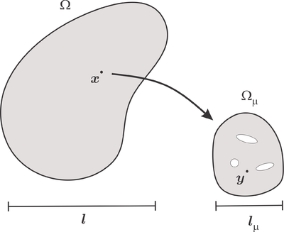

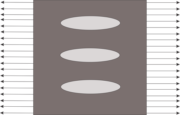
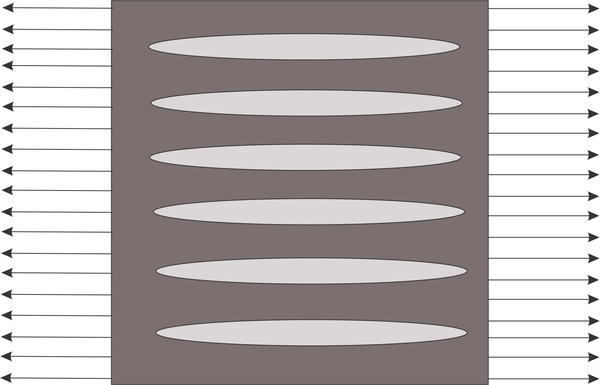
![Level-set function representation and its relation with the characteristic function (topology) [LevelSet2016]. Slight variations of the level-set function (assuming a small “off-set”) entail large differences on the topology.](/wd/images/thumb/f/f4/Draft_Samper_118254298-Level-set_image.png/600px-Draft_Samper_118254298-Level-set_image.png)
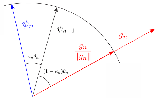
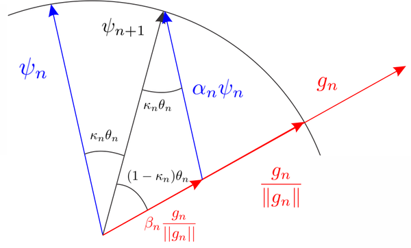

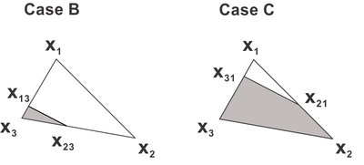

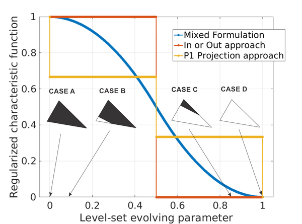
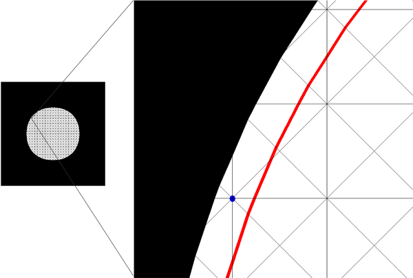

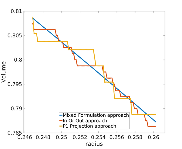
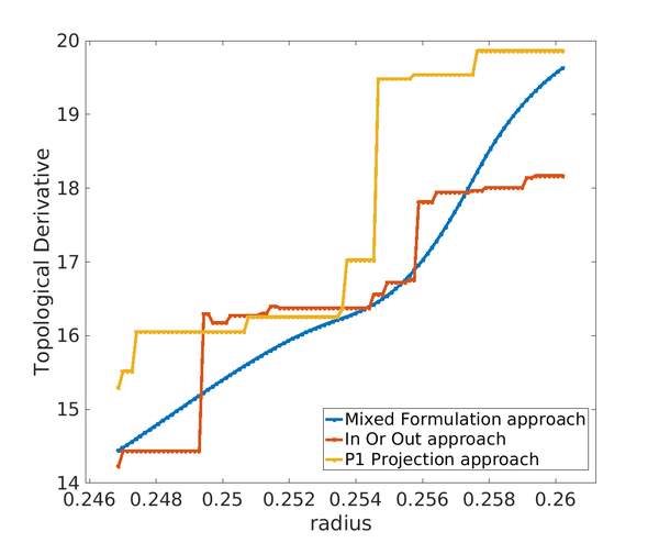


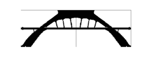
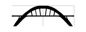
![Representative optimal homogeneous tension rod topologies: (a) Isotropic (E=1 and ν=0.3) as a reference, (b)-(e) Orthotropic, (f) Anisotropic. In the second column, the constitutive tensor used is shown, which is obtained by a classical homogenization procedure of the micro-structure displayed on the third column, see [Sanchez-PalenciaBook1980]. In the fourth one and fifth column, the final optimal topology for the structure and the value of the compliance are also shown.](/wd/images/thumb/d/d2/Draft_Samper_118254298_6711_TractionBeam.png/600px-Draft_Samper_118254298_6711_TractionBeam.png)
![Representative optimal homogeneous Cantilever beam topologies: (a) Isotropic (E=1 and ν=0.3) as a reference, (b)-(e) Orthotropic, (f) Anisotropic. In the second column, the constitutive tensor used is shown, which is obtained by a classical homogenization procedure of the micro-structure displayed on the third column, see [Sanchez-PalenciaBook1980]. In the fourth one and fifth column, the final optimal topology for the structure and the value of the compliance are also shown.](/wd/images/thumb/f/fc/Draft_Samper_118254298_4418_CantileverBeam.png/600px-Draft_Samper_118254298_4418_CantileverBeam.png)
