Abstract
Living biological tissues are complex structures that have the capacity of evolving in response to external loads and environmental stimuli. The adequate modelling of soft biological tissue behaviour is a key issue in successfully reproducing biomechanical problems through computational analysis.
This study presents a general constitutive formulation capable of representing the behaviour of these tissues through finite element simulation. It is based on phenomenological models that, used in combination with the generalized mixing theory, can numerically reproduce a wide range of material behaviours.
First, the passive behaviour of tissues is characterized by means of hyperelastic and finite-strain damage models. A generalized damage model is proposed, providing a flexible and versatile formulation that can reproduce a wide range of tissue behaviour. It can be particularized to any hyperelastic model and requires identifying only two material parameters. Then, the use of these constitutive models with generalized mixing theory in a finite strain framework is described and tools to account for the anisotropic behaviour of tissues are put forth.
The active behaviour of tissues is characterized through constitutive models capable of reproducing the growth and remodelling phenomena. These are built on the hyperelastic and damage formulations described above and, thus, represent the active extension of the passive tissue behaviour. A growth model considering biological availability is used and extended to include directional growth. In addition, a novel constitutive model for homeostatic-driven turnover remodelling is presented and discussed. This model captures the stiffness recovery that occurs in healing tissues, understood as a recovery or reversal of damage in the tissue, which is driven by both mechanical and biochemical stimuli.
Finally, the issue of correctly identifying the material parameters for computational modelling is addressed. An inverse method using optimization techniques is developed to facilitate the identification of these parameters.
1 Introduction
1.1 Motivation
Computational biomechanics is an emerging field that embraces a broad range of computational modelling techniques used in the numerical simulation and analysis of biological systems. Research in biomechanics, which seeks to understand the mechanics of living systems [3], is generally aimed at improving our knowledge of the human body to advance in medical science and technology. Unsurprisingly, biomechanics plays an important role in what is now termed in silico medicine [4]. This new discipline aims at capturing aspects of the physiology and pathology of the human body in computer models that aid in the clinical prevention, diagnosis and treatment of injury and disease. In this context, finite element analysis (FEA) [5] is proving to be a powerful tool to perform certain patient-specific biomechanical studies and, in this way, provide additional data for clinical decisions.
Computational biomechanics and in silico medicine overlap in areas such as orthopaedics, rehabilitation, gait analysis, tissue engineering, hemodynamics and mechanobiology, to name but a few. The latter is of particular interest for researchers in continuum mechanics and structural analysis since it poses the challenge of extending well-established constitutive formulations to be able to model biological tissue behaviour. Constitutive models describe the macroscopic behaviour resulting from the internal constitution of a material in order to characterize its response to external stimuli [6].
The constitutive modelling of biological tissues presents the difficulty of having to account for the fact that these materials are alive, so they respond and adapt to external and internal actions of both mechanic and metabolic origins. Furthermore, computational modelling of living tissues tends to involve complex and evolving geometries, large displacements and strains, and often their loads, boundary conditions and interactions are hard to quantify and establish with accuracy [7]. Further challenges include accounting for their hierarchical structure and the multiple biophysical stimuli at the different spatial and time scales involved.
1.2 Overview
Biological tissues are constituted by different components arranged in a hierarchical structure whose properties strongly depend on the size, distribution and geometry of these constituents. Biomaterials are typically classified into either hard or soft tissues. The former include mineralized tissues with a rigid intercellular substance, e.g., bone and teeth. They suffer small deformations and behave nearly elastically in the physiological range. The latter are tissues composed of an extracellular matrix (ECM) of collagen and elastin fibres embedded in ground substance. Examples of soft tissues are tendons, ligaments, skin, muscles and blood vessels, amongst others. They are highly deformable and exhibit a nonlinear elastic behaviour. In addition, the ground substance, which is basically a hydrophilic gel, confers near-incompressibility to these tissues.
The properties of both hard and soft tissues are classified into two separate groups, passive and active, according to their predominantly mechanical or biological nature. Properties that are not directly determined by the biochemical and biophysical processes taking place in the tissue are known as passive properties. In addition to the nonlinearity and near-incompressibility mentioned above, soft tissues may exhibit passive properties such as anisotropy, residual stresses, viscoelasticity, plasticity, damage and failure. In contrast, active properties are directly dependent on the metabolism, which keeps the tissues alive and allows them to adapt and evolve in response to their environment. Growth, atrophy, remodelling, healing, regeneration and ageing are all active properties.
Constitutive models to represent these properties can be developed following either a mechanistic or a phenomenological approach. The mechanistic approach tries to understand and model the mechanisms that regulate tissue reactions at cellular level. By incorporating the biophysics behind the tissue behaviour, these mathematical models allow testing different hypothesis and, ultimately, provide a better understanding of the mechanobiological interactions involved in the processes being modelled. However, they require in-depth knowledge of the tissue histology and the biochemical reactions taking place at cellular and molecular levels, which in some cases are not completely understood yet.
Phenomenological models, on the other hand, establish direct relations between the external stimuli and the observed tissue response without trying to explain the mechanisms behind the observations. They describe tissue behaviour using functional relations that closely fit experimental studies. The phenomenological approach avoids quantifying microscopic quantities. Instead, the internal variables of the model are directly associated with the behaviour observed at macroscopic level. These variables are expressed in continuous terms even though they are indirectly related to the mechanisms taking place at cellular and molecular levels. Nonetheless, biological tissues are extremely heterogeneous and, often, cannot be modelled with precision by using this approach alone.
The characterization of material inhomogeneity due to the local variation of the tissue structure is sometimes addressed with microstructural models. Histological data is used to describe the tissue architecture and then, by means of homogenization techniques, the macroscopic behaviour of the biomaterial is obtained. The underlying microstructural relations are mathematically complex and accurate quantification of the interactions between the constituents at the different organizational scales is required. Humphrey and Yin [8] proposed using mixing theory as an alternative, combining in this way desirable features from the phenomenological and microstructural approaches.
Mixing theory idealizes the composite material (the tissue) as composed of several individual compounds (fibres and matrix). Each of these components or simple materials is modelled, in turn, by the constitutive model of choice. Phenomenological models are generally used to describe the behaviour of the simple material, although mechanistic, microstructural or, even, mixing theory could be used for this purpose. The use of phenomenological models provides a compromise between the physical accuracy of the microstructural approach and the mathematical simplicity of the purely phenomenological one.
1.3 Goals
The aim of this study is to set the bases for a general constitutive formulation that represents the behaviour of soft biological tissues through numerical simulation, specifically, the finite element method (FEM). This formulation is based on phenomenological models used in combination with the generalized mixing theory [9] and implemented in the in-house code PLCd [1].
PLCd is an implicit FE code developed in Fortran and capable of solving finite-strain nonlinear three-dimensional solid mechanics problems. It uses the direct sparse solver Pardiso [10] and a full Newton algorithm. Originally developed for the modelling of fracture, dynamics behaviour and analysis of composite structures through mixing theory, its scope has extended over the years to topics such as multi-scale homogenization, fatigue analysis, the study of masonry structures and, now, biological tissue simulation. Among its strengths are the thorough implementation of the generalized mixing theory and the straightforward organization and accessibility of the code, which facilitates the introduction of new constitutive models. Nevertheless, since PLCd is research-oriented and in constant development, the implementation of new constitutive formulations often requires additional changes and improvements in the general structure of the code.
The mixing theory is understood as a constitutive equation manager that allows mixing and matching simple materials, whose behaviour is modelled by means of phenomenological constitutive formulations, to obtain the overall behaviour of the composite material. In this study, biological tissues are assimilated to a composite material and, therefore, the appropriate constitutive models must be formulated to represent its simple components. Hence, the idea of a general constitutive formulation for biological tissues: the use of mixing theory in conjunction with the simple constitutive models confers flexibility and versatility and, ultimately, generality to the overall formulation.
Exploiting the aforementioned strong points of the formulation, phenomenological constitutive models capable of reproducing biological tissue behaviour are developed and implemented in order to achieve the goal of this study, a general constitutive formulation. This task is tackled in two distinct parts: the passive and active properties.
First, the passive behaviour of biological tissues is addressed by means of quasi-incompressible hyperelastic and finite-strain damage models. This is, of course, a simplification since tissues are known to exhibit more complex behaviours such as viscoelasticity. However, the aim of the study is to obtain a general formulation and the hyperelastic and damage models are deemed enough for the purpose of representing the basic passive properties of the tissues.
Then, the active behaviour of the tissues is modelled through continuum growth and healing models, which are based on the previous hyperelastic and finite-strain damage formulations. Again, the active properties of living tissues include much more than the growth and remodelling modelled in this study. Yet, the scope of the general constitutive formulation is limited to these under the assumption that they are the most notable of the active properties observed in adult functional tissues.
The use of phenomenological models requires the correct identification of its material parameters to obtain an adequate computational representation of the real tissue behaviour. Due to the non-mechanistic nature of these parameters, it is often difficult to establish their values based on physical or structural information. Identifying the correct material parameters tends to require a trial-and-error approach, which is often tedious and generally time-consuming. Parameter identification through inverse methods by means of optimization techniques is an alternative to the manual identification. Such a method is developed, tailored to the particular applications of this study, but flexible enough to be easily modifiable if required for other purposes.
In view of the above, the aim of this study is divided into the following objectives, each of which corresponds to a chapter in this monography:
- Development of a set of constitutive formulations capable of representing the basic passive properties of biological tissues.
- Development of a set of constitutive formulations capable of representing the basic active properties of biological tissues.
- Identification of the material parameters of the constitutive formulations through an inverse method and adequate optimization techniques.
These constitutive formulations are developed in the framework of finite-strain continuum solid mechanics and are built on a well-established thermodynamic basis. The computational implementation and validation of the models require numerical improvements in areas of the code such as FE formulation, integration scheme, loading configurations and pre- and post-processor interfaces.
1.4 Outline
This monography is organized as follows:
Chapter 2 A set of constitutive equations capable of reproducing the basic passive properties of biological tissues is proposed. First, several hyperelastic formulations are reviewed and the implementation of two of these models is described in detail. The finite strain framework in which these formulations are developed and the numerical requirements imposed by the quasi-incompressibility assumption are also described. Then, a generalized finite-strain damage model is developed and implemented based on these hyperelastic models. A few examples serve to illustrate its main characteristics and validate the formulation. The use of these constitutive models together with generalized mixing theory is studied. Improvements to better represent the passive properties of biological tissues are proposed and discussed.
Chapter 3 A set of constitutive equations capable of reproducing the main active properties of biological tissues is proposed. Continuum modelling of growth and remodelling is reviewed and a constitutive model for volumetric growth that takes into account the metabolic contribution is described and implemented. An extension of this model to include directional growth is also presented. Then, a novel reverse-damage model to account for healing in soft tissues is formulated, implemented and validated through numerical examples. Similarly to the growth formulation, healing is driven by mechanical stimuli but subject to biological availability, as allowed by the tissue's metabolism. The integration of the growth and healing models in a common formulation in order to better represent the active properties of biological tissues is proposed and discussed.
Chapter 4 The constitutive formulation described in Chapter 2 is used to model the basic components of the human cervical spine and an attempt to numerically reproduce a discectomy spine surgery is presented. The difficulties encountered in the modelling of the spine are discussed and a solution is proposed to solve the material parameter identification problem. An inverse method using optimization techniques, tailored to this particular application, is developed. Then, the method is modified and used in the material parameter identification of a generic composite specimen, demonstrating the versatility of the method proposed. Finally, the improvements required in the cervical spine modelling are discussed, in addition to the capabilities of the proposed material parameter identification method.
Chapter 5 The achievements of this study are summed up, final conclusions are drawn and future work lines are outlined.
Note that a chapter devoted to reviewing the state of the art is not included at the beginning of the monography. The self-contained nature of each chapter lends itself to including specific literature reviews in each chapter. Likewise, conclusions related to the specific content of each chapter are pointed out at the end of the same.
1.5 Research dissemination
The work included in this monography resulted in the following scientific publications:
Chapter 2
- E. Comellas, F.J. Bellomo and S. Oller. A generalized finite-strain damage model for quasi-incompressible hyperelasticity using hybrid formulation. International Journal for Numerical Methods in Engineering, 2015. doi:10.1002/nme.5118.
Chapter 3
- F.J. Bellomo, E. Comellas, L. Nallim and S. Oller. Numerical simulation of the directioned growth and remodelling of soft biological tissues generated by mechanical stimuli (in Spanish). In: Mecánica Computacional Vol. XXXIII. Number 41. Computational Modeling in Bioengineering Applications (A), pages 2667–2676. Asociación Argentina de Mecánica Computacional, 2014.
- E. Comellas, T.C. Gasser, F.J. Bellomo and S. Oller. A homeostatic-driven turnover remodelling constitutive model for healing in soft tissues. Submitted to the Journal of the Royal Society Interface. October 2015.
Chapter 4
- E. Comellas, S. Oller, J. Poblete, J. Berenguer and A. Prats-Galino. Numerical modelling of a cervical spine discectomy. In: Mecánica Computacional Vol. XXXI. Number 24. Computational Modeling in Bioengineering and Biomedical Systems (A), pages 3811-3826. Asociación Argentina de Mecánica Computacional, 2012.
- E. Comellas, S.I. Valdez, S. Oller and S. Botello. Optimization method for the determination of material parameters in damaged composite structures. Composite Structures, 2015, 122:417–424. doi:10.1016/j.compstruct.2014.12.014.
In addition, part of the work was presented at the following conferences and workshops:
Unpublished Conference Presentations
- E. Comellas, T.C. Gasser, F.J. Bellomo and S. Oller. A reverse damage model for healing in soft biological tissues, VI International Conference on Computational Bioengineering (ICCB 2015), Barcelona, September 14 – 16, 2015.
- E. Comellas, F.J. Bellomo and S. Oller. Ogden parameter optimization for finite element modelling of cervical ligaments, invited to present in Biomechanics Session of XXXII Annual Conference of the Spanish Society of Biomedical Engineering (CASEIB 2014), Barcelona, November 26 – 28, 2014.
- E. Comellas, F.J. Bellomo and S. Oller. Ogden parameter optimization for finite element modelling of cervical ligaments using hybrid formulation, 11 World Congress on Computational Mechanics (WCCM XI), Barcelona, June 20 – 25, 2014.
Unpublished Workshop Presentations
- E. Comellas and S. Oller. Non-linear constitutive modelling of biological tissues, Course on Advanced Structural Analysis Interface, MuMoLaDe Michaelmas School a Marie Curie ITN, Barcelona, October 1 – 2, 2015.
- E. Comellas, T.C. Gasser, F.J. Bellomo and S. Oller. A damage-driven model for remodelling/healing of soft tissues considering biological availability, International Workshop on Modelling across the Biology-Mechanics Interface, Castro Urdiales, September 1 – 4, 2015.
- E. Comellas, F.J. Bellomo and S. Oller. Ogden parameter optimization for finite element modelling of cervical ligaments. IV Meeting of the Spanish Chapter of the European Society of Biomechanics (ESB), Valencia, November 20 – 21, 2014. Best valued works, 2 position.
- E. Comellas. TCAiNMaND Progress in WP5. TCAiNMaND First Annual Workshop, Barcelona, July 18, 2014.
- E. Comellas, F.J. Bellomo and S. Oller. FE modeling of cervical ligaments using Ogden hyperelasticity and hybrid formulation, III Meeting of the Spanish Chapter of the European Society of Biomechanics (ESB), Barcelona, October 23 – 24, 2013.
- E. Comellas, S. Oller, J. Poblete, J Berenguer and A. Prats-Galino. Numerical simulation of a cervical discectomy surgery (in Spanish), II Meeting of the Spanish Chapter of the European Society of Biomechanics (ESB), Sevilla, October 25, 2012.
Finally, part of the work presented in this document is the result of collaborating with external researchers during the following research stays:
- KTH Royal Institute of Technology, 6-month doctoral research stay. Worked under the direct supervision of Prof. Christian Gasser in the Solid Mechanics Department of the KTH Royal Institute of Technology. Stockholm, Sweden. February – July 2015. The article “A homeostatic-driven turnover remodelling constitutive model for healing in soft tissues” is the result of the work developed during the stay.
- CIMAT Center for Research in Mathematics, 2-month research stay in the framework of the TCAiNMaND project, a Marie Curie International Research Staff Exchange Scheme (IRSES) under the European Union 7 Framework Programme with grant agreement n. 612607. Worked under the direct supervision of Dr. Salvador Botello in the Computational Sciences Department of the Center for Research in Mathematics (CIMAT). Guanajuato, México. February – March 2014. The article “Optimization method for the determination of material parameters in damaged composite structures” is the result of the work developed during the stay.
2 Constitutive modelling of passive properties
2.1 Background
The adequate modelling of a biological tissue's constitutive behaviour is key in successfully reproducing biomechanical problems through computational analysis. The nonlinearity exhibited by soft tissue in response to loading was studied and experimentally quantified as early as mid-19th century [11]. The pioneering researchers in biomechanics observed that this behaviour is similar to that of rubber-like materials due to the long-chain, cross-linked polymeric structures of both types of materials. Hence, the introduction of continuum finite elasticity theory, used in the modelling elastomers, to model soft tissue behaviour.
Continuum-based theories deal with matter at a macroscopic scale, i.e., the behaviour of materials is studied considering matter as a continuous medium rather than as an heterogeneous mass formed by discrete particles. Also, the assumption is made that the solid and its properties are describable by continuous functions which have continuous derivatives. The existence of a continuous displacement field in this type of problems makes the implementation of finite element techniques to solve them much simpler.
Fung, considered by many the father of modern biomechanics, was among the first to characterize soft tissue biomechanics within the framework of finite-strain elasticity [12,3]. So, these first efforts to numerically reproduce soft tissue behaviour were mainly focused at determining the adequate elastic potentials or strain energy functions for such purpose.
Most of the models employed in representing soft tissue behaviour were borrowed or adapted, and still are, from elastomer applications. These models assume the material is homogeneous, nearly-incompressible and isotropic, which can be over-simplifying hypotheses for some biological tissues. Yet, these assumptions allow defining the elastic potential in terms of either the first and second invariant values of the right Cauchy-Green deformation tensor , or the principal stretches, which are the square roots of the eigenvalues of . This is especially useful in the mathematical development and numerical implementation of the hyperelastic formulation, as will be seen in section 2.2.
The main challenge is then to choose an appropriate set of invariants such that the material model includes as few parameters as possible but is still able to adequately reproduce complex deformation states of the material it is representing. In addition, the material parameters should be determined by fitting solely a small number of simple experiments. Among the most popular models of these type are the Mooney-Rivlin type, based on the first and second invariants of , and the Ogden models, based on the principal stretches. Another commonly used polynomial form of strain energy function is the one introduced by Yeoh, which uses power terms of the first invariant of . Exponential and logarithmic forms are also widely used, for example in the Fung and Veronda-Westmann models. The reader is referred to the comprehensive review on hyperelastic models for rubber-like materials by Steinmann et al. [13] for detailed information on many other constitutive models not mentioned in this study. Chagnon et al. [14] provide a comprehensive review of strain energy density functions for soft biological tissues. Studies of hyperelastic models for particular applications are also available, e.g. Auricchio et al. [15] review hyperelastic models for human aortic valve tissue.
The numerical and thermodynamic bases of isotropic quasi-incompressible hyperelasticity will be reviewed in section 2.2. The hyperelastic models typically used in biomechanical applications will be briefly described and discussed and, then, the complete neo-Hookean and Ogden formulations will be developed. Their numerical implementation in the in-house FE code PLCd [1] will be described and validated through numerical examples.
Although the hyperelastic models used to reproduce soft-tissue behaviour described above are able to adequately reproduce the behaviour of biological tissues in some applications, the anisotropy exhibited in most cases cannot be ignored. In order to address this issue, several authors [16,17,18] developed elastic potentials in terms of the components of the strain tensor. Therefore, the orientation of each material point in the tissue could be specified in terms of a certain coordinate system. Typically, the cylindrical polar coordinates are chosen for this purpose since these models were first applied on arterial tissue. However, this type of formulation is inherently limited to specific kinematics and the applicability of these models is limited, as discussed by Holzapfel [19].
Humphrey and Yin [8] proposed a different approach to modelling anisotropy. The elastic potential is defined as the sum of an isotropic part , attributable to the behaviour of the extracellular matrix (ECM), and an anisotropic one , accountable for the contribution of the collagen fibres. The latter, in turn, is defined as the sum of the contribution of each family of fibres 1. Then, the elastic potential of the tissue is
|
|
(2.1) |
where is the amount of fibre families considered. Here, is defined in terms of the right Cauchy-Green deformation tensor invariants and should account for the ECM behaviour. depends on both and the fibre orientation, typically through the pseudo-invariants of the fibre orientation vectors, also known as Spencer invariants [20]. The incorporation of the matrix-fibre distinction and the fibre orientation confers a certain mechanistic character to this formulation, even if phenomenological models are used as basis to define the basic elastic potentials.
Over the years, many researchers have used this same concept to develop constitutive models to represent soft tissue behaviour. One of the most popular of these models is the HGO model, developed by Holzapfel, Gasser and Ogden to represent arterial tissue behaviour [19]. Generally, the isotropic elastic potential is defined as an isotropic phenomenological hyperelastic function, while the definition of the anisotropic counterpart depends on the histological structure of the particular tissue being studied. Numerous constitutive formulations based on this isotropic/anisotropic split have been developed in the past decade and a half, extending the models to account for characteristics such as viscoelasticity [21,22,23,24,25], softening [26,27,28,29,30], or both [31,32].
Biological tissues exhibit several known softening phenomena: the Mullins effect, preconditioning, permanent set and damage softening [29]. The Mullins effect is a phenomenon originally investigated and documented by Mullins et al. [33] in rubbers. This effect is phenomenologically characterized by the degradation of the elastic properties of rubber-like materials subjected to quasi-static cyclic tensile/compressive loading. The degradation is observed at strain levels below the maximum strain achieved in the history of deformation. This stress-softening is associated with internal damage at microscopic level and structural realignment in the material. However, there is no general agreement on its physical source. Diani et al. [34] review both phenomenological and macromolecular models put forth by researchers in the field to model the Mullins effect in rubber-like materials. Preconditioning or hysteresis is characterized by an initial continuous softening in the first cycles of a testing procedure which is identically repeated on the same tissues [11]. Softening in the tissue halts when it reaches a steady or “saturated” state, that is, it suffers no further changes in its internal structure. Permanent set is the residual stretch observed in tissues after unloading [35]. Finally, softening in biological tissues may occur as a result of damage or degradation in the material structure. Rupture, fissures and voids at microscopic level occur in the tissue as the (macroscopic) deformation proceeds, resulting in an overall softening behaviour of the tissue.
The latter type of softening is commonly described through models formulated in a continuum damage mechanics (CDM) framework. These damage formulations are based on the hyperelastic strain energy functions, as will be seen in section 2.3. The CDM bases will be described in this section, together with a brief review of finite-strain damage models developed up to date, with particular focus on those developed for biological applications. Then, a general finite-strain damage model that can be particularized for any hyperelastic strain energy function will be developed and its numerical implementation and main characteristics will be described.
Let us recall the models based on a split elastic potential, initially introduced by Humphrey and Yin [8]. They can be interpreted as an ad hoc mixing theory, tailored to each biomechanical application. Now, since the aim of this study is to set the bases for a constitutive formulation to represent soft tissue behaviour, we propose a more general approach by directly using the generalized mixing theory [9], which works as a constitutive equation manager. In this way, one can build a library of constitutive equations which are known to adequately represent certain biological tissues or their main components and, then, choose the relevant models and quantify their contribution according to each application. So, there should be no need to redefine a new constitutive equation for each new biomechanical problem. The mixing theory is no longer introduced in the definition of the elastic potential, instead, it is applied at stress level. Then, for a tissue composed by distinct components (matrix and fibres), the second Piola-Kirchhoff stress in the tissue will be given by
|
|
(2.2) |
Here, is the volumetric participation of each tissue component and is the second Piola-Kirchhoff stress of each of these components, computed from its own constitutive equation.
The mixing theory formulation used, developed in a finite strain framework, will be reviewed in section 2.4. Its capability in reproducing soft tissue behaviour will be discussed as well as its shortcomings in the present form. In particular, the modelling of anisotropic behaviour in tissues will be addressed and the numerical tools that can be used to explicitly account for this behaviour will be discussed.
(1) Humphrey and Yin [8] define a family of fibres as “a collection of locally parallel fibres with identical material properties”.
2.2 Hyperelasticity
Hyperelastic models are basically higher-order forms of linear elastic ones and, therefore, are a particular type of nonlinear elastic models. Yet, hyperelasticity accounts for both nonlinear material behaviour and large geometric changes. Rubber-like materials are the most common example of a hyperelastic material but many elastomers and most soft biological tissues are also modelled using a hyperelastic idealization.
In elastic materials, the constitutive behaviour is solely a function of the current strain level or deformation state and does not depend on the loading path followed or the history of strains suffered by the material. This implies that the stress-strain curves for loading and unloading are exactly the same and, thus, the original shape of the material is recovered upon unloading. In other words, the work stored during loading is retrieved during the unloading process, so there is no dissipation of internal energy. Hence, strains are reversible and rate-independent, and there is a biunivocal correspondence between stress and strain.
The simplest elastic model is the linear elastic one, in which stress is directly proportional to strain through a linear relationship. However, in general, an elastic solid which undergoes large deformations will not follow linear elasticity. Many different constitutive relations can be developed to represent the behaviour of the elastic materials under the finite strain theory. In addition, the same constitutive behaviour, i.e., the same material model, can be written in several ways because of the different stress and deformation measures used in finite strain. These models are said to follow nonlinear elasticity and can be loosely grouped into [36,37,38]:
- Kirchhoff material. It is a straightforward generalization of linear elasticity to finite strain, typically used for applications in which the large deformation effects are due to geometric nonlinearities. The most general model is defined through the relation where is the second Piola-Kirchhoff stress tensor, is the constitutive tensor and is the Green-Lagrange strain tensor.
- Hypoelasticity. The constitutive equation is defined in terms of increments or rates, for example, , where is the rate of the Cauchy stress tensor, is the Cauchy stress tensor and is the rate of deformation tensor. These type of laws do not strictly reflect the path independence of elasticity. In addition, the derivation of objective stress rates 1 and the corresponding stiffness tensors is not trivial.
- Cauchy elasticity. The stress is computed by means of a material response function, , where is the deformation gradient tensor. The material response function has an explicit dependence on position, time and choice of reference configuration.
- Hyperelasticity or Green elasticity. Stress is obtained from a scalar specific strain energy density function, also known as Helmholtz free energy function or elastic potential, . This function is a measure of the energy stored in the deforming material such that, upon unloading, the energy is gradually released as the material recovers its original shape. The specific strain energy density function typically takes the form , although expressions for different stress measures are easily obtained through appropriate transformations.
The finite strain framework in which hyperelasticity is developed assumes that both rotations and strains are large and, thus, the reference or undeformed configuration is significantly different to the present or deformed one (see Figure 1). A clear distinction must be made between them and it is of utmost importance to know in which configuration one is working in at all times.
The implications of developing constitutive models for FEA in a finite strain framework are detailed in section 2.2.1. Then, the constraints imposed by the quasi-incompressibility of soft biological tissues in the numerical modelling are addressed in section 2.2.2. Section 2.2.3 presents the derivation of the basic constitutive formulation of quasi-incompressible hyperelasticity. Several hyperelastic models and their applicability to reproducing soft tissue behaviour are outlined in section 2.2.4. Then, the formulation derived in section 2.2.3 is particularized for the neo-Hookean and Ogden models in sections 2.2.5 and 2.2.6, respectively. The details of the numerical implementation in the in-house FE code PLCd [1] are described for both, and, finally, the numerical and modelling limitations of these two formulations are discussed in section 2.2.7.
(1) An objective stress rate is a time derivative of stress that is frame indifferent.
2.2.1 Finite strain framework
The great majority of solid mechanics FE solvers work with a Lagrangian mesh, and PLCd is no exception. This type of mesh is advantageous in computational solid mechanics because nodes and elements move with the material and, therefore, the problem boundaries and interfaces remain coincident with the element edges, simplifying their computational treatment. Also, the constitutive equations are evaluated always at the same material points because the integration points also move with the material and, thus, always coincide with the exact same point of the material. This is especially useful in history-dependent models such as damage, which will be addressed in section 2.3.
Then, the static equilibrium condition for an elemental discrete volume in the reference configuration is given by
|
|
(2.3) |
which must be satisfied for any displacement increment . Here,
- is the vector of residual forces, which must be null;
- , and are the reference volume, reference surface and reference density of the discrete volume, respectively;
- is the second Piola-Kirchhoff stress tensor;
- is the strain-displacement compatibility or transformation tensor, given by ;
- is the shape function;
- is the vector of body forces acting on the volume per unit of mass; and
- is the vector of surface forces acting on the surface of the volume per unit of surface.
The local equilibrium equations of each elemental volume are assembled in order to obtain the global equilibrium equation,
|
|
(2.4) |
where is a lineal operator that represents the sum of the different force components, according to the position and direction of the local contributions.
This equation may include nonlinearities, which can be of material or geometric origin. Material nonlinearities arise when the stress-strain behaviour is nonlinear due to the particular constitutive equation of the material. Constitutive nonlinearity is strictly due to the changes in the material properties during its mechanical behaviour. It is directly reflected in the constitutive tensor and, thus, the nonlinearity is introduced in 2.4 through the stress tensor . Geometric nonlinearities appear when there are changes in the geometry which have a significant effect on the load-deformation behaviour. In large displacement cases, the large translations and rotations taking place induce changes in the local reference system of the different solid points. This introduces nonlinearities in the displacement-strain compatibility tensor . Large strains, in addition to the large displacement effects, also introduce nonlinearities in the strain field due to the change in configuration of the solid. This change also modifies the constitutive tensor, which results in a nonlinear dependency of stresses on strains.
The reader is referred to reference textbooks in the FEM field such as Zienkiewicz and Taylor [5], Bathe [39], Crisfield [37] and Belytschko et al. [40] for detailed information on the numerical bases of nonlinear FE analysis.
FE solutions for problems which use Lagrangian meshes are typically divided into total Lagrangian (TL) and updated Lagrangian (UL) formulations. In both cases the dependent variables are functions of the material coordinates and time, i.e., they use Lagrangian descriptions. However, in the TL scheme all variables are referred to the reference (initial) configuration at time 0 whilst in the UL one they are referred to the current (deformed) configuration at time . Thus, in a TL formulation integrals are taken over the reference configuration and derivatives are calculated with respect to the material coordinates. In contrast, variables are integrated over the current configuration and derived with respect to spatial coordinates in an UL formulation. Nonetheless, both formulations include nonlinear effects due to large displacements, large rotations and large strains. Whether the large strain behaviour is modelled correctly or not will depend on the constitutive relations used and the results will be the same for both formulations if the appropriate constitutive models are defined in each formulation.
A decisive factor in choosing one formulation over the other is the computational efficiency. In the present study, the use of mixing theory might require the definition of angles to indicate the fibre alignment in the matrix. An UL approach would require updating the angle information, as well as the integration volumes, each time the equilibrium of forces were to be enforced. This was regarded as a considerable computational drawback and the decision was made to use a TL framework. However, because one might need to define certain constitutive equations in the reference configuration, a partially updated Lagrangian (pUL) framework was implemented. In the pUL framework, all steps of the resolution scheme are performed in the reference configuration, except for the computation of the stress tensor through the constitutive equation, which is done in the present configuration (see Figure 2). To switch between the two configurations, push-forward and pull-back operators, denoted as and , respectively, are required. These are defined as
|
|
(2.5) |
where is the Kirchhoff stress tensor, is the Jacobian determinant and is the Euler-Almansi strain tensor.
![Scheme of the total Lagrangian and partially updated Lagrangian formulations implemented in PLCd [1]. The subindex k indicates iteration number in the present load increment. The definition of each term is available in the notation list.](/wd/images/thumb/1/17/Draft_Samper_593843246-picture-cb7e7b.png/600px-Draft_Samper_593843246-picture-cb7e7b.png)
|
| Figure 2: Scheme of the total Lagrangian and partially updated Lagrangian formulations implemented in PLCd [1]. The subindex indicates iteration number in the present load increment. The definition of each term is available in the notation list. |
2.2.2 Quasi-incompressibility and hybrid elements
The near-incompressibility characteristic of many tissues is attributed to the high volume fraction of water present in most soft tissues [11]. Hence, soft tissue behaviour is typically represented through quasi-incompressible hyperelastic models, albeit the adequacy of the quasi-incompressibility hypothesis of soft tissues has been debated in some cases [41,42].
Assuming soft tissue behaviour can be modelled by means of quasi-incompressible hyperelasticity implies that any hydrostatic pressure can be applied on said material without changing its shape and, thus, stress cannot be uniquely determined from strains. In this case, the hyperelastic constitutive law only specifies the deviatoric stresses and the hydrostatic stresses must be calculated by solving the equilibrium equations with the appropriate boundary conditions (assuming a quasi-static loading case). Thus, the specific strain energy density function in the reference configuration is split into
|
|
(2.6) |
where corresponds to the volume-preserving or volumetric part and , to the isochoric or deviatoric one [43].
In addition, a quasi-incompressible material has a quasi-infinite bulk elastic modulus, which results in an ill-conditioned stiffness matrix and locking problems when computing the solution using standard displacement-based FE formulations.
Gadala [44] reviews in his work the formulations proposed to overcome these difficulties, detailing the advantages and disadvantages of one approach over another. All of them are based on the decomposition of the deformation gradient into a deviatoric or isochoric part and a volumetric or dilatational one. The most popular approaches used in literature can be grouped into:
- Multifield or mixed principles. The variational principle behind the FE formulation not only includes the displacement field, but also the volumetric deformation and/or pressure fields [45,43]. In their most general form, they have the disadvantage of introducing a considerable number of unknowns into the problem, which is computationally costly. However, static condensation at element level can eliminate the pressure degrees of freedom and, thus, this problem is overcome [39].
- Reduced selective integration penalty approach. The displacement field corresponding to the deviatoric deformation is integrated normally but the volumetric terms are integrated using low order rules [46]. This reduces the over-stiffening caused by volumetric locking. Unfortunately, this approach does not work well with elements subjected to large strains or highly distorted elements [44].
In the present work, a two-field approach has been used. The u/p formulation described by Crisfield [37] and Bathe [39], consisting in a mixed interpolation of the displacements and pressure has been implemented into PLCd [1]. This formulation is based on the classical displacement FEM but includes an additional unknown variable, the hydrostatic stress distribution or pressure, which is interpolated separately from the displacement variable [46]. Then, the equations of motion for an elemental discrete volume are
|
|
(2.7) |
where is the displacement vector, is the pressure vector, are the stiffness matrices and and are the vector of forces corresponding to the external and internal loads, respectively. All variables are nodal and given in the reference configuration. The stiffness matrices are defined as , which results in
|
|
(2.8) |
|
|
(2.9) |
and
|
|
(2.10) |
Here and are the classical linear and nonlinear strain-displacement compatibility or transformation tensors, respectively [2]. is the tangent constitutive tensor, is the vector of pressure shape functions, is the bulk modulus and is a vector which in matrix form is the pressure-related constitutive tensor . The internal forces are computed as
|
|
(2.11) |
and
|
|
(2.12) |
where is the pressure obtained from the displacement field and is the total element pressure obtained by independent interpolation, . Then, and are constitutive tensors relating strain and pressure, respectively, to stress, i.e.,
|
|
(2.13) |
The pressure constitutive tensor is given by
|
|
(2.14) |
where is the right Cauchy-Green deformation tensor that is defined in terms of the deformation gradient tensor as . Since the volumetric part of the Cauchy stress tensor is given directly by the hydrostatic pressure 1, , the pressure constitutive tensor is, in fact, a pull-back operation 2.5 of this term. So, converts the Cauchy stress to Kirchhoff stress () and, through the inverse of the right Cauchy-Green deformation tensor, the pull-back operation is completed.
Now, the pressure obtained from the displacement field, , is defined positive in compression and computed as
|
|
(2.15) |
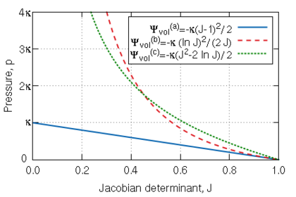
where can take different forms according to different authors [39,37,43,47], but is always defined in terms of the Jacobian determinant , which is a measure of the change of volume, and the bulk modulus . Possible functions of and their corresponding function for the pressure are
|
|
(2.16) |
In the first case, , the value of the bulk modulus directly dictates the value of the pressure when there is no change in volume, i.e., (see Figure 3). In addition, the tetrahedral elements that will be discussed later are very sensitive to the choice of the function . In this sense, the best choice is the one with the term because it usually has a stabilizing effect [48]. For these reasons, the first expression in 2.16 of the volumetric specific strain energy density function has been used in PLCd [1]. Then, the internal force corresponding to the volumetric part is reduced to
|
|
(2.17) |
where has been taken into account.
|
| Figure 3: Pressure (positive in compression) vs. the Jacobian determinant for the different volumetric specific strain energy density functions given in 2.16 in terms of the bulk modulus . |
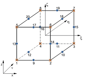
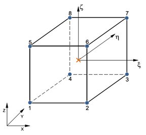
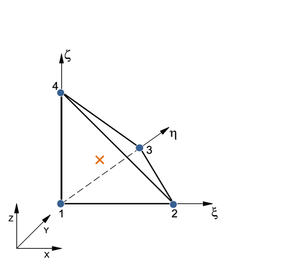
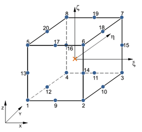
Figure 4 shows two possible configurations of mixed elements based on the serendipitous hexahedral and the tetrahedral families of elements already implemented in PLCd [1]. Both element types satisfy the inf-sup condition 2 and, therefore, will produce robust and reliable solutions. Figure 5 shows alternative configurations of the distribution of the pressure nodes in which these nodes do not coincide with the displacement nodes. Such elements are often referred to as hybrid elements and have the advantage of allowing for static condensation of the pressure variables in the equation of motion. Isolating from the second line of 2.7 yields
|
|
(2.18) |
which, replaced into the first line of 2.7, results in the condensed equation of motion to be solved,
|
|
(2.19) |
The formulation obtained is expressed solely in terms of displacement variables, and the new stiffness tensor and internal force vector differ from the classic displacement FE formulation in that they have the pressure-related subtracting terms. Therefore, the same FE solver can be used because new variables have not been added, only the stiffness tensor and internal force vector require modification.
|
![Possible configurations for mixed u/p elements that satisfy the inf-sup condition [39]: elements Q2P1c (left) and P2P1c (right). The blue circles indicate displacement nodes and the orange crosses indicate pressure nodes. Nodes are numbered according to the local numbering criterion used in PLCd [1].](/wd/images/thumb/8/8c/Draft_Samper_593843246-P2P1c.png/288px-Draft_Samper_593843246-P2P1c.png)
|
| Figure 4: Possible configurations for mixed u/p elements that satisfy the inf-sup condition [39]: elements Q2P1c (left) and P2P1c (right). The blue circles indicate displacement nodes and the orange crosses indicate pressure nodes. Nodes are numbered according to the local numbering criterion used in PLCd [1]. | |
|
|
|
![Possible configurations for mixed u/p or hybrid elements that allow for static condensation of the pressure variables in the equation of motion. Elements Q1P0 (top left) and T1P0 (top right) do not satisfy the inf-sup condition. Elements Q2P0 (bottom left) and T2P0 (bottom right) satisfy the inf-sup condition but the constant pressure assumption may require fine discretization [39]. The blue circles indicate displacement nodes and the orange crosses indicate pressure nodes. Nodes are numbered according to the local numbering criterion used in PLCd [1].](/wd/images/thumb/1/1d/Draft_Samper_593843246-P2P0.png/288px-Draft_Samper_593843246-P2P0.png)
|
| Figure 5: Possible configurations for mixed u/p or hybrid elements that allow for static condensation of the pressure variables in the equation of motion. Elements Q1P0 (top left) and T1P0 (top right) do not satisfy the inf-sup condition. Elements Q2P0 (bottom left) and T2P0 (bottom right) satisfy the inf-sup condition but the constant pressure assumption may require fine discretization [39]. The blue circles indicate displacement nodes and the orange crosses indicate pressure nodes. Nodes are numbered according to the local numbering criterion used in PLCd [1]. | |
Now, not all possible configurations of hybrid elements shown in Figure 5 perform equally. Element Q1P0 does not satisfy the inf-sup condition but is capable of predicting reasonably good displacements and is commonly used because of its simplicity. However, due to the constant pressure assumption, stress predictions may be inaccurate [39]. Element T1P0 is known to exhibit volumetric locking for nearly incompressible deformations and most authors recommend directly avoiding its use in problems of this type [37,49,38]. Nonetheless, tetrahedral linear elements present considerable advantages in terms of computational cost and straightforward meshing of complex geometries. This motivated some authors [50,51,52] to develop the averaged nodal pressure tetrahedral element, which overcomes the volumetric problems of the standard T1P0 element. This option was studied for PLCd [1] but eventually discarded since it was seen that quadratic tetrahedrons do not entail an excessively high computational cost for the applications we could consider modelling with this code. Elements Q2P0 and T2P0 both satisfy the inf-sup condition but, again, fine discretization may be required in order to accurately predict stresses due to the constant pressure assumption. To overcome this problem, linear or quadratic pressure variable distributions can be introduced but, to obtain adequate results, switching to higher order displacement distributions is also required [39]. Thus, Q1P0, Q2P0 and T2P0 elements are deemed to be sufficient for the purposes of this study.
When a constant pressure distribution is considered, the condensed equation of motion 2.19 is further simplified. There is a single pressure variable, therefore, , and the pressure shape function vector is reduced to . Then, the stiffness matrices 2.9 and 2.10, and internal force vector 2.12 become
|
|
(2.20) |
|
|
(2.21) |
|
|
(2.22) |
The definition of the pressure constitutive tensor 2.14 has been taken into account in 2.20.
Figure 6 summarizes the condensed mixed u/p formulation implemented in PLCd [1] for the total Lagrangian framework. Extension to the partially updated Lagrangian framework is straightforward and requires no additional changes (see Figure 2).
![Scheme of the condensed mixed u/p or hybrid formulation implemented in PLCd [1] for a total Lagrangian framework (reference configuration). The subindex k indicates iteration number in the present load increment. The definition of each term is available in the notation list.](/wd/images/thumb/0/05/Draft_Samper_593843246-picture-b1c7c4.png/600px-Draft_Samper_593843246-picture-b1c7c4.png)
|
| Figure 6: Scheme of the condensed mixed u/p or hybrid formulation implemented in PLCd [1] for a total Lagrangian framework (reference configuration). The subindex indicates iteration number in the present load increment. The definition of each term is available in the notation list. |
(1) Here, is the second-order identity tensor, which is defined as , being the Kronecker delta function.
(2) The inf-sup condition is the basic mathematical criterion that determines whether a mixed finite element discretization is stable and convergent and, hence, will yield a reliable solution [39].
2.2.3 Thermodynamic basis of hyperelastic formulations
The Axiom of Local State postulates that, in continuous media, the thermodynamic state at a given point and time instant is completely defined by a certain number of variables at that time instant. The physical phenomena can be described with precision depending on the nature and number of state variables chosen for that. The process defined in this way will be thermodynamically admissible if, at any time instant, the Clausius-Duhem inequality 1 is satisfied. The state variables, also named thermodynamic or independent variables, are the observable and the internal variables. Internal variables describe the internal structure of the medium, which is hidden to the eye of the external observer who simply sees a “black box”. It must be pointed out, though, that the notion of internal depends upon the considered level of observation: a variable considered as internal from the point of view of macroscopic observation will probably be an observable variable from a mesoscopic point of view. Thus, the tensor and physical nature of the internal variables should be known. Furthermore, these variables are, in practice, measurable but not controllable.
It follows that the dependent values in the continuous medium such as stress are, at any given time instant, a function of both the values of the independent observable variables and the internal variables. In the particular case under consideration, the observable variables are strain, , and temperature, , whilst no internal variables are considered. We anticipate that, in the following section, when damage is introduced, there will be an internal variable associated with the damage in the material, .
Once the state variables have been defined, one postulates the existence of a thermodynamic potential from which the state laws can be derived. This potential must be a continuous scalar function, concave with respect to the temperature, convex with respect to the other state variables and containing the origin. Taking the Helmholtz free energy, one has . Then, the local form of the second law of thermodynamics in terms of internal specific energy density is expressed through the Clausius-Duhem inequality in reference configuration [54] as
|
|
(2.23) |
where is the specific entropy, is the heat flux vector and is the dissipation. Considering solely purely deformation processes where there does not intervene any changes in entropy or temperature, and taking into account that hyperelastic materials have null internal dissipation due to the reversible character of their loading processes, this equation is reduced to
|
|
(2.24) |
Then, the time derivative of the energy function is described in terms of the second Piola-Kirchhoff stress tensor and its conjugate, the rate of Green-Lagrange strain as . The rate of energy, which is totally due to deformation, is equal to the stress power. Expanding the derivative of the energy function leads to
|
|
(2.25) |
which shows that, as expected, derives from a strain energy function. It is often more convenient to use the right Cauchy-Green deformation tensor instead of the Green-Lagrange strain tensor. Introducing the relation , the stress results in
|
|
(2.26) |
This relation can be expressed using other stress tensors such as the first Piola-Kirchhoff stress tensor, . If one recalls that, like and , the tensors and are work conjugates, then
|
|
(2.27) |
In any case, the elastic potential must fulfil:
- Normalization condition: the function must be zero when the material is completely unloaded, .
- The energy function must grow monotonously with deformation, .
Additionally, a reversible material (with no internal energy dissipation) must also satisfy:
- The work performed by the forces must be independent of the path followed, .
- For any closed deformation cycle, the deformation work must be zero, .
Now, introducing the additive split of the specific strain energy density function 2.6 into 2.26, and considering the first volumetric specific strain energy density function in 2.16, yields the constitutive equation
|
|
(2.28) |
Here, the relation has been considered in the derivation of . This constitutive equation must now be completed by defining an appropriate deviatoric part of the specific strain energy density function, . Many different functions have been proposed over the years in order to adequately represent the behaviour of the material being modelled. These must satisfy the aforementioned conditions of the elastic potential in addition to the principle of material frame-indifference 2. The isotropic functions typically used in biomechanical applications will be reviewed in the following section.
An isotropic material exhibits identical behaviour in all material directions. In mathematical terms, isotropy requires 2.26 to be independent of the chosen material axes. Thus, the specific strain energy density function must be defined solely in terms of the invariants of the right Cauchy-Green deformation tensor,
|
|
(2.29) |
The invariants of are defined as
- First invariant: ,
- Second invariant: ,
- Third invariant: ,
and the corresponding partial derivatives, which will prove useful in the derivation of the different hyperelastic constitutive equations, are
- ,
- and
- .
Expressions of isotropic specific strain energy density functions given in the present configuration are generally defined in terms of the invariants of the left Cauchy-Green deformation tensor . This tensor, also known as Finger deformation tensor, is defined as and is known to have identical invariants to those of the right Cauchy-Green deformation tensor: , and .
Finally, let us evaluate the rate of change of the constitutive equation 2.28, which can be expressed as
|
|
(2.30) |
Here, is a symmetric fourth-order tensor named tangent constitutive tensor, tangent stiffness or elasticity tensor. It can be noted that, even though this expression is similar to Hooke's Law (), here the tangent constitutive tensor is not constant but a function of strain, and it relates the material time derivatives of strain and stress. Because the stress and strain variables belong to the reference configuration, this tensor is known as the Lagrangian or material elasticity tensor. The equivalent tensor in current configuration is obtained if a push-forward operation is performed on the time derivatives of stress and strain. This yields the Eulerian or spatial elasticity tensor, , which relates the Lie derivative 3 of the Euler-Almansi strain to the Lie derivative of the Kirchhoff stress,
|
|
(2.31) |
The spatial elasticity tensor is, in fact, the push-forward of the material one which, in index notation, is written as
|
|
(2.32) |
The tangent constitutive tensor is used to obtain the stiffness tensor by means of 2.8. The correct implementation of the tangent constitutive tensor is of particular importance in highly nonlinear models because an error in its numerical formulation can lead to lack of convergence in the calculation, especially in problems involving triaxial stress states.
Introducing the additive split of the specific strain energy density function 2.6 into 2.30 yields the material tangent constitutive tensor
|
|
(2.33) |
Considering the first volumetric specific strain energy density function in 2.16 for the volumetric tangent constitutive tensor results in
|
|
(2.34) |
where the operator is used to indicate the open product between the two second-order terms. Further developing this expression in terms of the right Cauchy-Green deformation tensor invariants produces
|
|
(2.35) |
Here, the fourth-order tensor is defined as
|
|
(2.36) |
Performing the push-forward operation 2.32 on 2.35, yields the volumetric part of the spatial elasticity tensor,
|
|
(2.37) |
where the fourth-order identity tensor is defined as
|
|
(2.38) |
The last terms in 2.35 and 2.37 are not included in the definition of the tangent tensor at constitutive level. This term corresponds to the purely volumetric component of the tangent constitutive tensor and is already accounted for separately at element level in the implementation of the hybrid element (see section 2.2.2).
The deviatoric part of the tangent constitutive tensor must be derived for each hyperelastic model according to the expression of its particular . Unfortunately, this is not always an easy task. Alternatively, the complete tangent constitutive tensor, or only its deviatoric part, can be computed numerically through the perturbation technique outlined by Miehe [55].
(1) The Clausius-Duhem inequality is a way of expressing the second law of thermodynamics in local form which is extensively used in continuum mechanics. This inequality is particularly useful in determining whether the constitutive relation of a material is thermodynamically allowable [53].
(2) The principle of material frame-indifference, also referred to in literature as material objectivity, requires that the constitutive equations not depend on the external frame of reference used to describe them or, in other words, the constitutive equations should be independent of the observer.
(3) To perform a time derivative of a variable in the current configuration, this variable must be first pulled-back to the reference configuration. The material time derivative is performed and, then, the variable is brought back to the current configuration through a push-forward. This is so because the derivative must be performed in an invariant frame. The Lie derivative is defined [19] as the change of a spatial field relative to the vector field : .
2.2.4 Characterization of soft biological tissue behaviour using hyperelasticity
The specific strain energy density functions most commonly used in modelling soft biological tissue behaviour are presented in this section. These correspond to the deviatoric part of the elastic potential in 2.6, however, the tilde has been dropped in this section for simplicity. The expression for uniaxial stress is also given for each model and is then employed in a simple example to illustrate the characteristics of each model.
The deformation gradient tensor obtained when loading uniaxially in the -direction is
|
|
(2.39) |
where is the stretch in the loading direction, defined as . Here, is the original length and is the deformed (stretched) length. Then, the second Piola-Kirchhoff stress in the loading direction is derived from the specific strain energy density function following
|
|
(2.40) |
Note that because the third invariant is due to the near-incompressibility assumption. Here, the expressions and have been used. Finally, the first Piola-Kirchhoff and Cauchy stresses in the loading direction are obtained through the transformations and , respectively.
Neo-Hooke It is the simplest hyperelastic model, given by the specific strain energy density function [56]
|
|
(2.41) |
where is a material constant related to the initial shear modulus of the material, . Then,
|
|
(2.42) |
is the corresponding second Piola-Kirchhoff stress in the loading direction of an uniaxial loading set-up.
Mooney-Rivlin The general form of the specific strain energy density function [57,58] for this model is
|
|
(2.43) |
where are the material constants and is a positive integer that determines the order of the model. Then,
|
|
(2.44) |
is the corresponding second Piola-Kirchhoff stress in the loading direction of an uniaxial loading set-up for the first-order model (). It is usually assumed that and , yet may be positive and still result in a positive-definite specific strain energy density function [59]. The first-order model with becomes the neo-Hookean model. The stress for the second-order model () is
|
|
(2.45) |
In general, higher order models are not as used since they require fitting a considerable amount of material constants to the experimental data.
Yeoh This model is defined by the specific strain energy density function [60]
|
|
(2.46) |
where , and are material constants. The initial shear modulus is given by . Then,
|
|
(2.47) |
is the corresponding second Piola-Kirchhoff stress in the loading direction of an uniaxial loading set-up.
Fung The specific strain energy density function of this model [3] is
|
|
(2.48) |
where and are the positive material constants related to the shear modulus and the stiffening, respectively. Then,
|
|
(2.49) |
is the corresponding second Piola-Kirchhoff stress in the loading direction of an uniaxial loading set-up.
Veronda-Westmann This model adds a term based on the second invariant of to the exponential term of the Fung model that depends solely on the first invariant of this tensor. Thus, the specific strain energy density function [61] is given by
|
|
(2.50) |
where , and are material constants. Then,
|
|
(2.51) |
is the corresponding second Piola-Kirchhoff stress in the loading direction of an uniaxial loading set-up.
Ogden The specific strain energy density function [62] is based on the principal stretches, instead of the invariants of ,
|
|
(2.52) |
Here, the shear moduli and the stiffening parameters must satisfy the consistency condition
|
|
(2.53) |
is a positive integer that determines the order of the model. The third-order model is the most widely used, although the first-order model () with reduces to the Neo-Hookean expression and the second-order model () with and produces the Mooney-Rivlin expression. For the third-order model,
|
|
(2.54) |
corresponds to the second Piola-Kirchhoff stress in the loading direction of an uniaxial loading set-up.
As a general rule, a model with more parameters has a higher chance of producing a good fit to experimental data. The drawback is, of course, identifying the adequate parameter values. A model with a large amount of material parameters may be burdensome and time-consuming to fit. Therefore, the simplest model which gives a reasonable fit to the desired experimental data is usually selected for a given application. Experimental data that includes several types of test (uniaxial, biaxial, torsion, etc.) tends to require more complex models in order to correctly reproduce the tissue behaviour.
Figure 7 shows the stress-stretch responses for the hyperelastic models described above, whose material parameters have been fitted to experimental data of liver tissue under tensile and compressive loadings [63]. The values used for these parameters are given in Table 1. The fitting was performed manually through trial and error and does not pretend to be an exhaustive study but merely an illustrative example. The reader is referred to the comprehensive studies of hyperelastic material models for modelling biological tissue behaviour by Martins et al. [64] and Wex et al. [65] for more information on this subject.
![Uniaxial stress-stretch responses for the different hyperelastic models used to fit the experimental data [63] of liver tissue under tensile and compressive loadings. The material parameters in Table 1 have been used.](/wd/images/thumb/e/e1/Draft_Samper_593843246-1PK_ALLhyper.png/570px-Draft_Samper_593843246-1PK_ALLhyper.png)
|
| Figure 7: Uniaxial stress-stretch responses for the different hyperelastic models used to fit the experimental data [63] of liver tissue under tensile and compressive loadings. The material parameters in Table 1 have been used. |
| Model | Param. | Value |
| Neo-Hooke | ||
| Mooney- | ||
| Rivlin | ||
| Mooney- | ||
| Rivlin | ||
| () | ||
| Yeoh | ||
| Model | Param. | Value |
| Fung | ||
| Veronda- | ||
| Westmann | ||
| Ogden | ||
The neo-Hookean and first-order Mooney-Rivlin models are clearly incapable of reproducing the J-shape of the stress-stretch curves characteristic of soft tissue behaviour. Nonetheless, they are typically used when the stretches of interest are in the initial linear interval of the tissue response due to their simplicity and ease in fitting. In addition, it is often used to represent the ECM behaviour in the context of mixing theory constitutive formulations.
The most popular hyperelastic models for representing soft tissue behaviour are the Fung and Yeoh models because they predict responses with reasonable accuracy and require a small amount of parameters. The Veronda-Westmann model produces comparable results but has not received as much attention in literature.
The third-order Ogden model generally produces accurate fits but requires identifying six material parameter values. Yet, its use in soft tissue modelling is also considerably extended owing to the fact that it is based on the principal stretches, which are directly measurable quantities.
Precisely for this reason, the Ogden hyperelastic model has been chosen for implementation in PLCd [1]. In addition, it can be easily reduced to the neo-Hookean and first-order Mooney-Rivlin models with adequate values of its material parameters. The neo-Hookean model has also been implemented in the code since it is the most basic and simple of hyperelastic models.
2.2.5 Neo-Hookean hyperelasticity
The neo-Hookean function 2.41 is introduced as the deviatoric term in the split specific strain energy density function 2.6, resulting in
|
|
(2.55) |
where the first expression in 2.16 has been taken into account for the volumetric part of the elastic potential. Here, the material constant is related to the initial shear modulus through , is the bulk modulus and is the modified volume-preserving first invariant of .
As expected, if there is no deformation and . Then, the elastic potential vanishes since and .
Applying 2.28, the constitutive equation in the reference configuration
|
|
(2.56) |
is obtained. Performing a push-forward operation 2.5 on this expression, the constitutive equation in the present configuration results in
|
|
(2.57) |
Considering the split definition 2.33 of the material elasticity tensor and the expression of its volumetric part 2.35 corresponding to the selected volumetric elastic potential, the material elasticity tensor is computed as
|
|
(2.58) |
where has been introduced and the the fourth-order tensor is computed as in 2.36.
Then, the spatial elasticity tensor
|
|
(2.59) |
is obtained by applying the push-forward operation 2.32 on 2.58. The fourth-order identity tensor is defined in 2.38.
The tangent constitutive tensor in the reference and present configurations both satisfy the minor and major symmetries and , respectively.
The terms containing the bulk modulus in 2.58 and 2.59 are not included in the definition of the tangent tensor at constitutive level when hybrid elements are used. This term corresponds to the purely volumetric component of the tangent constitutive tensor and is already accounted for separately at element level in the implementation of the hybrid element (see section 2.2.2). In addition, the tangent constitutive tensor in a pUL framework could be directly computed in the reference configuration instead of computing and then performing a pull-back to obtain . In the pUL framework, the calculation of the stiffness tensor is performed in the reference configuration and, therefore, requires instead of (see Figures 2 and 6).
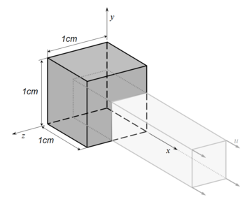
The scheme at Gauss point level of the numerical integration in PLCd [1] of the isotropic neo-Hookean hyperelastic model is outlined in Table 2. The implementation has been validated by means of a simple example consisting in a single element subjected to homogeneous uniaxial tensile loading. An 8-noded hexahedral element with 1cm length sides and a single pressure point (Q1P0) is subjected to a displacement-driven pure tensile load applied in steps of 0.1mm (see Figure 8). The material constant has been set to 27.2kPa and a penalizer value of Pa has been considered for the bulk modulus . The results for both TL and uPL formulations coincide with the reference curve from [64] and are shown in Figure 9.
| Algorithm at each load increment
Given: deformation gradient tensor , elemental pressure and the material property .
|
|
| Figure 8: Prescribed displacements applied on an 8-noded hexahedral linear element with a single pressure integration point (Q1P0) used in the homogeneous uniaxial tensile test example. |
![Results for an 8-noded hexahedral linear element with a single pressure integration point (Q1P0) under homogeneous uniaxial tensile loading. Neo-Hookean hyperelastcity with C₁=27.2\,\textrmkPa and a penalizer value κ=10¹²\,\textrmPa has been considered. PLCd [1] results for both TL (blue crosses) and pUL (green squares) formulations coincide with the reference results from [64] (black line).](/wd/images/thumb/6/6c/Draft_Samper_593843246-Hooke-uni.png/366px-Draft_Samper_593843246-Hooke-uni.png)
|
| Figure 9: Results for an 8-noded hexahedral linear element with a single pressure integration point (Q1P0) under homogeneous uniaxial tensile loading. Neo-Hookean hyperelastcity with and a penalizer value has been considered. PLCd [1] results for both TL (blue crosses) and pUL (green squares) formulations coincide with the reference results from [64] (black line). |
A second example reproducing a membrane with a hole at its centre subjected to tensile loading is performed to ensure the correct numerical implementation of the formulation. The membrane depicted in Figure 10 is subjected to the indicated displacement-driven loading . Due to the symmetry in the specimen, only a quarter of the membrane has been discretized using 360 hexahedral elements. Symmetry conditions are imposed, thus, nodes belonging to the symmetry plane shown in Figure 10 have motion restricted in the direction, while nodes belonging to the symmetry plane have motion in the direction restricted. Accumulative incremental displacements are imposed in the direction on the nodes of the top part of the specimen, with the other directions left unrestrained. The material constant has been set to 7.5kPa and a penalizer value of Pa has been considered for the bulk modulus .
The mechanical response for the TL formulation is illustrated in Figure 11 (top left) by means of the vertical reaction vs. stretch curve. The vertical reaction plotted is the total resultant reaction force in the direction of the quarter of the specimen. Figure 11 (bottom) shows the pressure and the principal second Piola-Kirchhoff stress distribution for the final displacement value mm. The convergence curves for each load increment, plotted in Figure 11 (top right), show adequate convergence of the solution. A tolerance of of has been used and only two iterations per load increment are required to reduce the maximum residue below this value.
The same example is repeated with quadratic hexahedral (Q2P0) and tetrahedral (T2P0) meshes (see Figures 12 and 13). The tetrahedral mesh contains elements whose side lengths are, on average, half the side length of the hexahedral element. Table 3 summarizes the characteristics of each mesh.
| Element type | Total number of elements | Gauss points per element | Total number of nodes |
| Q1P0 | 360 | 8 | 630 |
| Q2P0 | 360 | 27 | 2217 |
| T2P0 | 39458 | 4 | 14739 |
2.2.6 Ogden hyperelasticity
The specific strain energy density function of the third-order Ogden hyperelastic material 2.52 is introduced as the deviatoric term in the split specific strain energy density function 2.6, resulting in
|
|
(2.60) |
Here, the first expression in 2.16 has been taken into account for the volumetric part of the elastic potential. The shear moduli , and , and the stiffness constants , and are empirically determined material constants that must satisfy the consistency condition 2.53. The volume-invariant or deviatoric principal stretches , and are related to the principal stretches through with and .
Then, applying 2.28, the constitutive equation in the reference configuration
|
|
(2.61) |
is obtained. Here, the tensor is given by , where is the eigenvector of the right Cauchy-Green deformation tensor such that . In addition, the square of the principal stretches are the eigenvalues of , i.e., . The scalar is related to the deviatoric principal stretches through
|
|
(2.62) |
Performing a push-forward operation 2.5 on 2.61 and considering that yields
|
|
(2.63) |
which corresponds to the constitutive equation in the present configuration. Here, is defined as in 2.62 and the tensor is given by , where is the eigenvector of the left Cauchy-Green deformation tensor, i.e., . Analogous to the reference configuration, the square of the principal stretches are the eigenvalues of , i.e., .
Considering the split definition 2.33 of the material elasticity tensor and the expression of its volumetric part 2.35 corresponding to the selected volumetric elastic potential, the material elasticity tensor is computed as
|
|
(2.64) |
Here, has been introduced, the fourth-order tensor is computed as in 2.36 and the scalar is related to the deviatoric principal stretches through
|
|
(2.65) |
The term is given by
|
|
(2.66) |
where the fourth-order identity tensor is defined in 2.38. Here, the scalar is computed as and its derivative is .
Then, the spatial elasticity tensor
|
|
(2.67) |
is obtained by applying the push-forward operation 2.32 on 2.64. The term is given by
|
|
(2.68) |
where the fourth-order tensor is defined as
|
|
(2.69) |
The reader is referred to the work by Simo and Taylor [43] for further details on the derivation of the constitutive equation and tangent constitutive tensor from the Ogden hyperelastic specific strain energy density function.
As in the neo-Hookean model, the tangent constitutive tensor in the reference and present configurations both satisfy the minor and major symmetries. Again, the terms containing the bulk modulus in 2.64 and 2.67 are not included in the definition of the tangent tensor at constitutive level since they correspond to the purely volumetric component that is already accounted for separately at element level in the implementation of the hybrid element (see section 2.2.2).
The scheme at Gauss point level of the numerical integration in PLCd [1] of the isotropic third-order Ogden hyperelastic model is outlined in Table 4. The implementation has been validated by means of a simple example consisting in a single element subjected to homogeneous uniaxial tensile loading. An 8-noded hexahedral element with 1cm length sides and a single pressure point (Q1P0) is subjected to a displacement-driven pure tensile load applied in steps of 0.1mm (see Figure 8). The material constants have been set to , , , , and . A penalizer value of Pa has been considered for the bulk modulus . The results for both TL and uPL formulations coincide with the reference curve from [66] and are shown in Figure 14.
| Algorithm at each load increment
Given: deformation gradient tensor , elemental pressure and material properties and for .
|
![Results for an 8-noded hexahedral linear element with a single pressure integration point (Q1P0) under homogeneous uniaxial tensile loading. Ogden hyperelasticity with μ₁=12.069\,\textrmPa, μ₂=3.773\,\textrmMPa, μ₃=-52.171\,\textrmkPa, α₁=8.395, α₂=1.882, α₃=-2.2453 and a penalizer value κ=10¹². PLCd [1] results for both TL (blue crosses) and pUL (green squares) formulations coincide with the reference results from [66] (black line).](/wd/images/thumb/8/80/Draft_Samper_593843246-Ogden-uni.png/366px-Draft_Samper_593843246-Ogden-uni.png)
|
| Figure 14: Results for an 8-noded hexahedral linear element with a single pressure integration point (Q1P0) under homogeneous uniaxial tensile loading. Ogden hyperelasticity with , , , , , and a penalizer value . PLCd [1] results for both TL (blue crosses) and pUL (green squares) formulations coincide with the reference results from [66] (black line). |
A second set of examples are performed to ensure the correct numerical implementation of the formulations. The membrane with a hole subjected to displacement-driven loading (see Figure 10) in the previous section 2.2.5 is now modelled with Ogden hyperelasticity. The material constants considered are , , , , and , in addition to a penalizer value . Again, the example has been repeated with three different meshes, each of which uses a different type of hybrid element (see Table 3).
The mechanical response of the TL formulation for the Q1P0 mesh is illustrated in Figure 15 (top left) by means of the vertical reaction vs. stretch curve. The vertical reaction plotted is the total resultant reaction force in the direction of the quarter of the specimen. Figure 15 (bottom) shows the pressure distribution and the principal second Piola-Kirchhoff stress distribution for the final displacement value mm. The convergence curves for each load increment, plotted in Figure 15 (top right), show adequate convergence of the solution. A tolerance of has been used and, again, only two iterations per load increment are required to reduce the maximum residue below this value. Figures 16 and 17 show these results for the Q2P0 and T2P0 meshes, respectively.
2.2.7 Discussion
The neo-Hookean and Ogden hyperelastic models have been implemented successfully in PLCd [1] for both TL and uPL formulations, as confirmed by the validation examples provided. Both models produce practically the same results regardless of the configuration (reference or present one) chosen for the definition of the constitutive equation. These two definitions of a same model are, strictly speaking, different constitutive equations that reproduce a same behaviour.
The pUL formulation used requires a series of push-forwards and pull-backs that the TL one does not require. This obviously increases the overall calculation time and might induce numerical errors which could explain the slightly delayed convergence in the pUL examples reproducing complex stress states. For this reason, when possible, the TL formulation will be favoured over the pUL one. On occasions, a constitutive model, or the parameters defining a constitutive model, could be only available in the present configuration. In such case, the use of the pUL would be mandatory.
The analytical constitutive tensors have been implemented correctly since a low number of iterations per load step is required in all examples. In future models that might not allow for the analytical derivation of their constitutive tensor, the calculation by perturbations [55] will be required although this will certainly increase the computational cost.
Regarding the element order, lineal elements are known to be inadequate for the analysis of problems involving bending [49]. However, refining the mesh can improve substantially the quality of the results. Quadratic elements will always yield better results than their linear counterparts but, of course, are computationally more expensive. On the other hand, when the geometry allows it, hexahedral elements should be favoured over tetrahedral ones as they produce much better results using fewer elements and, hence, less computation time.
The fact that the hybrid elements used all have a single pressure point might translate into unrealistic stress distributions. A constant pressure per element results in an approximately constant volumetric stress per element, which means the stress is no longer continuous across elements. In addition, the incompressibility condition is enforced at elemental level and, thus, the individual Gauss points of a same element might have slight volume changes which even out at elemental level. The Cauchy and Kirchhoff stresses are obtained through a push-forward operation on the second Piola-Kirchhoff stress, which uses the deformation gradient tensor and its determinant. Then, these volume differences are reflected in the stress distribution at the present configuration. Applying a smoothing technique on the stress distribution in the post-processing with GiD [67] of the results reduces the visibility of this effect (see Figure 18), although the best solution would undoubtedly be to implement mixed elements with higher number of pressure integration nodes.
Nonetheless, the single pressure elements Q1P0, Q2P0 and T2P0 already implemented in the code will be used in the remainder of this study. The linear element Q1P0 will be favoured when possible owing to its computational efficiency. The aim of this study is to develop a constitutive formulation for representing the behaviour of biological tissues. Thus, the shortcomings of these elemental formulations are acknowledged, but it is not the purpose of this study to address them.

|

|

|
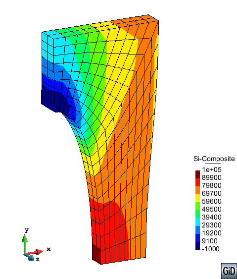
|

|

|
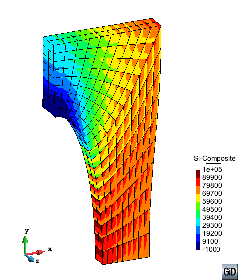
|
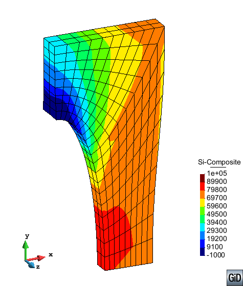
|
| Figure 18: Stress distributions at an imposed displacement value of mm for the membrane with a hole modelled using neo-Hookean hyperelasticity in a TL framework and meshed with Q1P0 elements (above, see Figure 11) and Q2P0 elements (below, see Figure 12). Principal second Piola-Kirchhoff stress (left), smoothed principal second Piola-Kirchhoff stress (centre left), Kirchhoff stress (centre right) and smoothed Kirchhoff stress (right) distributions. Real deformation (1) is plotted. | |
2.3 Finite-strain damage
A damaged material is characterised by a certain loss of load carrying capacity with respect to the original, undamaged material. This damage is a result of micro-voids and small fissures, present inside the matter, starting to grow. As they increase in size, there is a progressive material deterioration which can be measured through a loss in strength and stiffness [68]. This deterioration culminates in crack initiation, growth and final fracture. The latter are, obviously, occurring at larger scales than the material imperfections overlooked when dealing with continuum mechanics. Therefore, continuum concepts are somewhat difficult to introduce here. However, for the former phase, the process of progressive material deterioration leading up to the initial crack formation, a continuum approach can be followed to model the behaviour of the damaged material.
Continuum damage mechanics (CDM) is used to describe the progressive degradation experienced by the mechanical properties of materials prior to the initiation of macro-cracks. The small fissures and micro-voids occurring before are modelled as continuous, disregarding the discontinuity they introduce into the material properties but taking into account how they globally affect the value of these properties. The theories developed in the continuum damage framework are based on the thermodynamics of irreversible processes and use internal state variables [69]. They offer complementary possibilities to fracture mechanics, which deals with the actual fracture phenomena and requires the modelling of the cracks and voids present in the material.
The extent of damage in a given material is not directly measurable as strain is in elasticity and an alternative must be found in order to quantify the damage. The effective stress tensor is introduced, which interprets the change in mechanical behaviour of a damaged material as a loss of effective area. Thus, a damage variable that is, in general, a tensor quantity is defined. Denoted by , this fourth-order tensor characterises the state of damage in an anisotropic model and transforms the “real” stress tensor, , into the effective stress tensor,
|
|
(2.70) |
The concept of effective stress was first introduced in 1958 by Kachanov [70] through the use of a reduction factor associated with the amount of damage in the material. This factor would be equal to unity at the initial moment when no damage was present and reduce to zero, either at the moment of fracture localization or at the moment of rupture. In addition, a hypothesis of strain equivalence can be introduced. It states that “the strain associated with a damaged state under the applied stress is equivalent to the strain associated with its undamaged state under the effective stressâ [69], as illustrated in Figure 19.
![Schematic illustration of the effective stress concept, adapted and reproduced with permission from Oller [104].](/wd/images/thumb/e/ee/Draft_Samper_593843246-Dam_StressEquiv.png/540px-Draft_Samper_593843246-Dam_StressEquiv.png)
|
| Figure 19: Schematic illustration of the effective stress concept, adapted and reproduced with permission from Oller [104]. |
In the case of isotropic damage, the mechanical behaviour of the small cracks and voids is completely independent of their orientation and affects the material properties in the exact same way, whichever material direction is considered. This, however, does not necessarily imply that the original undamaged constitutive tensor of the material is isotropic. The isotropic damage simply preserves the directional characteristics of the initial elastic tensor by degrading it equally in all directions and, therefore, is describable by a single scalar variable . In this model, the internal damage variable is rewritten as , where is the fourth-order symmetric identity tensor defined in 2.38. Then, 2.70 becomes
|
|
(2.71) |
where the damage parameter is a measure of the loss of rigidity in the material and must be within the limits . A value of represents an undamaged material state whilst represents a material state such that the material is completely degraded. This state can represent anything ranging from initial (macro)crack formation to local rupture, depending on what one defines as full material damage.
Since Kachanov first introduced the concept of effective stress, many authors have developed formulations based on this concept of elastic degradation to model damage in materials. Over the years, these formulations have consolidated and are now regarded as indisputable knowledge in the context of CDM [71,69,68,72]. This phenomenological approach is based on a rigorous mathematical and thermodynamic basis that will be reviewed in section 2.3.1. This formulation has proved to be a simple and effective tool in numerical modelling. Although initially formulated in an infinitesimal strain framework and as isotropic, it has been extended to include anisotropy [73,74], has been combined with plasticity [75,76,77] and viscoelasticity [78], and has been formulated for application to specific materials such as concrete [79,80], composites [81] or biological tissues [82], among others.
The first damage models developed in a finite strain context were proposed more than two decades ago, being the work of Simo [69] one of the most renowned. These are generally based on the additive decomposition of the specific strain energy density function (introduced for hyperelasticity in section 2.2.2) with damage affecting only the deviatoric part. Like the formulations by Miehe [83], de Souza [84] and other authors [34], these models were motivated by the Mullins effect (see section 2.1). More recently, damage models based on the decoupled volumetric-deviatoric response have been formulated to model the behaviour of fibred soft biological tissues [28,85,30,86,87]. The main characteristics of some of these models will be reviewed in section 2.3.2.
All these formulations use damage criteria and evolution laws which are defined to particularly suit the specific material behaviour being modelled. In this work, a generalized finite-strain damage softening model is proposed, which includes linear and exponential damage evolution laws that have been translated from an infinitesimal strain framework [9] into the present finite strain one. The novelty of this formulation is that, on the one hand, both proposed evolutions of the damage variable are based on solely two measurable material properties and, on the other hand, the formulation can be particularized for any decoupled volumetric-deviatoric hyperelastic constitutive model desired. Thus, the result is a general-purpose formulation which is versatile enough to model disparate material behaviours without requiring reformulation of the damage model or complex material parameter adjustments. The details of the proposed model are presented and discussed in sections 2.3.3 through 2.3.5.
2.3.1 Thermodynamic basis of finite-strain damage formulations
Damage models based on the split elastic potential definition with damage affecting solely the deviatoric part of the elastic potential associate the damage mechanism with the maximum distortional energy of the material and assume damage is independent of hydrostatic pressure [88]. Following this hypothesis [19], the specific strain energy density function is
|
|
(2.72) |
where is the undamaged isochoric or deviatoric part and is its undamaged volumetric one, both given in the reference configuration. The Jacobian determinant is related to the right Cauchy-Green deformation tensor, , through . The tilde in indicates that it is the deviatoric or volume-preserving part of , given by . The functions chosen for and must be such that and hold if and only if and , respectively.
Expression 2.72 introduces an internal scalar damage variable , which defines a reduction factor similar to the one first proposed by Kachanov [70].
For an isothermal case with uniform temperature distribution and other standard arguments [88], the Clausius-Duhem inequality in the reference configuration 2.23 is reduced to
|
|
(2.73) |
where is the second Piola-Kirchhoff stress tensor. Considering , the expression becomes
|
|
(2.74) |
Then, introducing the specific strain energy density function defined in 2.72 and rearranging, the internal dissipation in the reference configuration
|
|
(2.75) |
is obtained. This inequality must hold true for any strain increment, therefore, the term in brackets must be null and the expression of the dissipation is reduced to
|
|
(2.76) |
Setting the term in brackets in 2.75 to zero yields
|
|
(2.77) |
which is the finite-strain version of the Kachanov effective stress concept. Here, the same volumetric specific strain energy density function used in hyperelasticity 2.28 has been introduced.
Consider now the material tangent constitutive tensor 2.33 and the expression for its volumetric part derived in 2.34. Then, a general expression for the material elastic-damage tangent constitutive tensor is derived as with
|
|
(2.78) |
Now, the onset and evolution of the damage variable in the constitutive equation 2.77 must be defined to complete the finite-strain damage model.
2.3.2 Characterization of soft biological tissue behaviour using finite-strain damage
Various models based on this approach have been proposed for characterizing the degradation or damage in biological tissues since the foundations of the finite-strain damage formulation were first developed in the 1980s.
Among the major known causes of physiological damage in biological tissues are the tensile and shearing structural failures due to the relative motions between tissue components [89]. Damage in soft tissues is caused by fibre tearing and rupture caused by excessively high stretches. Collagen fibres are, in fact, a bundle of collagen fibrils assembled together by proteoglycan cross-links. As stretch on the fibre increases, the proteoglycan cross-links begin to rupture, weakening the collagen fibre [31]. This results in the stress-stretch response shown in Figure 20. Initially, the collagen fibres in the tissue are crimped and most of the loading is borne by the ECM (I: toe region). As loading progresses, the fibres begin to straighten and start to bear load. The fibres are said to be “recruited”. The high nonlinearity observed (II: heel region) and fast increase in stiffness value is due to more and more fibres being recruited. Once all fibres have been recruited, a constant stiffness region ensues (III: linear region) in which fibres are completely straightened and at full load-bearing capacity. At certain loading, fibres reach their maximum possible extension and start to rupture. At first, only a few fibres are disrupted and the tissue as a whole can still continue bearing load, albeit with a lower stiffness (IV: progressive fibre failure). Fibres continue to rupture as loading on the tissue increases, reaching a point where the tissue can no longer bear any loading. The tissue stiffness suddenly decreases just before complete rupture of the tissue (V: complete failure).
![Schematic illustration of fibred soft tissue response to loading, inspired by [94]. (I) Toe region: ECM bears most of the loading, the tissue exhibits low value of practically constant stiffness. (II) Heel region: Fibres are progressively recruited, the stiffness of the tissue increases in a nonlinear manner. (III) Linear region: The majority of fibres have been recruited, the tissue has a high value of nearly constant stiffness. (IV) Progressive fibre failure: Fibres weaken and start to rupture, slightly decreasing the overall stiffness of the tissue. (V) Complete failure: The majority of fibres have ruptured, the tissue decreases drastically its load-bearing capacity until it completely fails.](/wd/images/thumb/2/27/Draft_Samper_593843246-Damage_tissue.png/420px-Draft_Samper_593843246-Damage_tissue.png)
|
| Figure 20: Schematic illustration of fibred soft tissue response to loading, inspired by [94]. (I) Toe region: ECM bears most of the loading, the tissue exhibits low value of practically constant stiffness. (II) Heel region: Fibres are progressively recruited, the stiffness of the tissue increases in a nonlinear manner. (III) Linear region: The majority of fibres have been recruited, the tissue has a high value of nearly constant stiffness. (IV) Progressive fibre failure: Fibres weaken and start to rupture, slightly decreasing the overall stiffness of the tissue. (V) Complete failure: The majority of fibres have ruptured, the tissue decreases drastically its load-bearing capacity until it completely fails. |
Therefore, damage in soft tissue is related to the microstructural response of the tissue to loading. From a CDM viewpoint, the fibre rupture and ECM disruption can be assimilated to the small fissures and micro-voids observed in damaging inert materials and, hence, the justification for using CDM theory to model damage in soft tissue. Constitutive models that take into account the mechanisms causing damage at fibrilar level have been proposed [31,87]. Yet, a common approach from a phenomenological perspective is to describe fibre rupture and ECM disruption by means of adequate mathematical expressions of damage onset and evolution. These models mainly vary in how damage is defined to begin and evolve.
It must be noted that the hypothesis assumed here, namely, that damage affects solely the deviatoric part of the elastic potential, has been questioned by some researchers in the field. On the one hand, there is the debated issue of the quasi-incompressibility behaviour of soft tissues, attributed to the high volume fraction of water present in most soft tissues [11]. For supra-physiological loadings, the injury produced could potentially introduce changes in the water content of the tissue, which would require revisiting the quasi-incompressibility assumption and, hence, the use of a split elastic potential. On the other hand, accounting for the possibility of cavitational damage arising in soft tissues [90,91] would mean defining a damage model that exclusively affects the volumetric part of the material definition. For the purposes of the present study, damage will be considered to affect only the deviatoric part of the elastic potential, albeit the aforementioned limitations of this modelling approach.
Continuous and discontinuous damage variables Most authors define damage in terms of a discontinuous variable, , such that the reloading and the unloading response of the model coincide. Thus, damage accumulation never occurs for strain values below the previous maximum attained strain. A typical form of discontinuous damage variable is
|
|
(2.79) |
where is the history variable [83,84].
Miehe [83] introduced a continuous damage variable into the definition of the total damage, . Then, part of the damage accumulates continuously within the deformation process, even during unloading and reloading at strain values below the previous maximum. The continuous damage variable is defined in terms of the arc-length of the undamaged strain energy function as
|
|
(2.80) |
where the initial condition is . Miehe worked in an exclusively spatial setting, but the formulation can be extrapolated to a TL framework. The continuous damage variable has been used for modelling the Mullins effect [92,93] and preconditioning [30,94] in biological tissues. Conversely, to account for the softening exclusively caused by damage (rupture) in soft tissues, researchers usually use a discontinuous damage variable.
Decoupled tensile-compressive models The damage model described in the previous section 2.3.1 has been developed based on the effective stress concept. In other words, the model is based on the hypothesis that damage is directly linked to the history of total strains and, in addition, damage is accumulative in nature. To illustrate this concept, consider the fact that, once the material starts to fissure and micro-voids appear, it is impossible that they later reduce their size and disappear. Thus, damage can grow but will never diminish. Nonetheless, it could happen that, if these small fissures and micro-voids are closed (due to a posterior compressive load state for example) they will not affect the macroscopic behaviour. Then, the damaged state is still present but it is considered to be passive, as opposed to the active state when the damage in the material is growing [68]. If the loading state were subsequently reversed and a tensile load applied again, the damage state would be the previously existing one before it would continue degrading. To account for this phenomena, models in which the specific strain energy density function [95] or the strain tensor [82] is decomposed into its tensile and compressive parts are used and damage is made to affect only the tensile one.
Onset and evolution of damage The evolution of the discontinuous damage variable is given by
|
|
(2.81) |
where is a non-negative scalar named damage consistency parameter used to define the loading, unloading and reloading conditions through the Karush-Kuhn-Tucker complementary conditions
|
|
(2.82) |
The damage surface is
|
|
(2.83) |
where is a damage evolution law given in terms of the norm , and is a scalar function of the damage threshold , which is the maximum reached value of in the history of strains. The damage criterion proposed by Simo and Ju [69],
|
|
(2.84) |
is quite extended [28,96,35,85], although other functions of the specific strain energy density function are also used [97,98].
Numerous expressions have been proposed for the damage evolution law to characterize damage in soft tissue. Among the type of functions used are exponential [82,97,98,28,93,29,99], root [95], polynomial [96,100] and sigmoidal [101,29] ones. The reader is referred to the article by Peña [85] for a detailed review on the topic. Some of these functions are tailored to particular applications and their parameters can be assigned a physical meaning [27,99]. These functions tend to have a considerable amount of material parameters which are not always easily obtainable from experimental data. Other functions are more phenomenological in nature and require fitting fewer parameters [82,95], although they may not have a direct physical meaning. The functions proposed by Balzani and coworkers [98,30,102] and Calvo, Peña and coworkers [28,100,32,85] in general rely on only two or three material parameters which have been proven to show excellent fit with experimental data. In addition, some of the functions include viscosity, directional damage, separate fibre and matrix contributions and/or other softening effects such as preconditioning, permanent set and the Mullins effect.
In this work, for the purpose of setting the bases of a general constitutive formulation that represents the passive behaviour of soft tissues, the finite-strain extension of two evolution laws first described in an infinitesimal strain context are proposed. These are developed with the aim of reproducing a wide range of softening behaviours and are to be used in conjunction with mixing theory. Thus, they must be simple in their formulation, easy to fit to experiments and versatile enough to reproduce disparate soft tissue behaviour. The damage laws proposed use a discontinuous damage variable since they only aim to represent softening due to damage. Also, damage will be isotropic and affect equally the tensile and compressive states. Possible ways to account for anisotropy and different tensile/compressive behaviours in tissues will be addressed at composite level in section sec:RoM.
2.3.3 Proposed damage evolution laws
The linear and exponential explicit scalar functions described in [103,104] as damage evolution laws in an infinitesimal strain context have been translated to a finite strain framework to define . A notable advantage of these laws is that they are based on only two material parameters with direct physical sense that can be experimentally determined.
Linear softening The damage variable is defined as a scalar function with linear arguments
|
|
(2.85) |
where and are the material properties initial damage threshold and fracture energy per unit volume, respectively. Both may be obtained from experimental uniaxial tensile tests as in classical damage models [105]. In particular, the initial damage threshold is computed as
|
|
(2.86) |
where is the stored elastic energy up to the elastic limit corresponding to the uniaxial initial damage threshold stress and calculated as shown in Figure 21. The parameter in 2.85 is a dissipation-related parameter obtained by imposing
|
|
(2.87) |
Introducing 2.76 and 2.85 into the previous equation yields
|
|
(2.88) |
Considering the Simo and Ju criterion in 2.84 and introducing integration by parts, this expression becomes
|
|
(2.89) |
The damage variable has been defined for the interval , therefore
|
|
(2.90) |
Then, 2.89 results in
|
|
(2.91) |
and, considering 2.87, the parameter
|
|
(2.92) |
is obtained.
Exponential softening The damage variable is defined as a scalar function with exponential arguments
|
|
(2.93) |
The parameter is obtained in a similar manner to the parameter in the linear softening law. Up to 2.89 the procedure is identical. Then, the damage variable, defined for the interval , is now
|
|
(2.94) |
Since is always true, it becomes obvious that for . Thus, operating on 2.89 with these values of and yields
|
|
(2.95) |
and, considering 2.87, the parameter
|
|
(2.96) |
is finally obtained.
Tangent constitutive tensor The expression for the material tangent constitutive tensor derived in 2.78 can now be completed. Specifically, the term becomes
|
|
(2.97) |
where the Simo and Ju criterion 2.84 has been taken into account. Then, the volumetric and deviatoric parts of the tangent constitutive tensor 2.78 are now
|
|
(2.98) |
Here, the differentiation of the evolution law with respect to the energy norm is
|
|
(2.99) |
for the linear softening law 2.85 and
|
|
(2.100) |
for the exponential softening one 2.93.
2.3.4 The generalized finite-strain damage model
The damage model for quasi-incompressible hyperelasticity proposed [106] is developed in a total Lagrangian finite strain framework following CDM theory and uses a Kachanov-like reduction factor applied on the deviatoric part of the hyperelastic constitutive equation, as shown in 2.77. The linear and exponential softening laws, 2.85 and 2.93, respectively, are proposed to describe the evolution of damage. The corresponding tangent constitutive tensor is derived in 2.98. The damage model proposed can be particularized for any hyperelastic model based on the volumetric-isochoric split of the Helmholtz free energy. However, for the present study it has been implemented in the in-house FE code PLCd [1] for neo-Hooke and Ogden hyperelasticity (see sections 2.2.5 and 2.2.6, respectively).
Particularization for neo-Hookean hyperelasticity Introducing the deviatoric part of the stress 2.56 defined in the neo-Hookean hyperelastic model, the constitutive equation 2.77 becomes
|
|
(2.101) |
Here, the material constant is related to the initial shear modulus through and is the bulk modulus.
Introducing now the corresponding deviatoric part of the material elasticity tensor 2.58, the tangent constitutive tensor 2.98 becomes
|
|
(2.102) |
Here, the fourth-order tensor, has been defined in 2.36.
Particularization for Ogden hyperelasticity Introducing the deviatoric part of the stress 2.61 defined in the Ogden hyperelastic model, the constitutive equation 2.77 becomes
|
|
(2.103) |
where is related to the deviatoric principal stretches through
|
|
(2.104) |
The tensor is given by , where is the eigenvector of . The material parameters and are the (constant) shear moduli in the reference configuration and dimensionless stiffening constants, respectively, and both must satisfy the consistency condition 2.53.
Considering now the corresponding deviatoric part of the material elasticity tensor 2.64, the tangent constitutive tensor 2.98 becomes
|
|
(2.105) |
Here, the fourth-order tensor is already defined in 2.36, the scalar is related to the deviatoric principal stretches through
|
|
(2.106) |
and the derivative has already been given in 2.66.
The numerical integration in PLCd [1] at Gauss point level of these particularizations of the generalized finite-strain damage model presented is outlined in Table 5. As in the hyperelastic models, the last term in the volumetric component of the tangent constitutive tensors 2.102 and 2.105 is not included in the definition of the tangent tensor at constitutive level. This term corresponds to the purely volumetric component of the tangent constitutive tensor and is already accounted for separately at element level in the implementation of the hybrid element (see section 2.2.2).
| Initialization at and
Damage =, dissipation and maximum reached value of the damage threshold stress, . Algorithm at each load increment Given: deformation gradient tensor , elemental pressure , hyperelastic material properties and damage material properties and .
Verification of the damage threshold criterion:
|
| and |
Calculation of the dissipation To ensure the damage model implemented is thermodynamically consistent, the total dissipation value of the structure, , can be numerically obtained by means of expression 2.76 through
|
|
(2.107) |
When damage localizes in a band of elements, can be compared to an estimate of the same value calculated in terms of the fracture energy, taking into account 2.87, and the final volume of the elements in the damaged band as
|
|
(2.108) |
Here, the maximum dissipated fracture energy per unit volume, , is related to the material property , which is the maximum dissipated fracture energy per unit area, through the element's characteristic length in the reference configuration, : . The final volume can be computed as , where is the final cross-section area of the band of elements where damage has localized and is the final length of these elements in the direction perpendicular to . Finally, defining a final damage stretch as , the expression for the total dissipation results in
|
|
(2.109) |
Imposition of initial damage It might be of interest in some computational applications to impose a certain damage in part of the structure and then study its evolution to an applied loading. The sole difficulty in introducing an initial damage value lays in correctly updating the maximum reached value of the damage threshold at the beginning of the problem. The initial damage threshold remains unchanged as it is a material property.
Because the damage law is an explicit function of the damage threshold , the equation can be equated to the imposed damage value and the corresponding value is isolated. Then, for linear softening 2.85 the initial should be
|
|
(2.110) |
and for exponential softening 2.93 it should be
|
|
(2.111) |
where the Lambert function is defined as .
So, in the numerical integration scheme of Table 5 the damage variable will no longer be initialized to zero but to the value . And the initial value of the maximum reached value of the damage threshold will be calculated according to the equations above. The initial damage option has been implemented in PLCd [1] in such a way that different elements can be assigned different values of initial damage ranging from 0 to 1 (both included). However, in the sake of simplicity, all integration points in a given element are assigned the exact same value.
The main characteristics of the proposed damage model are presented by means of two representative three-dimensional examples. A homogeneous state under uniaxial tension is reproduced with the aim of illustrating the basic constitutive characteristics of the damage formulation for both the neo-Hookean and the Ogden particularizations of the formulation. Then, a membrane with a hole at its centre is subjected to a tensile load in order to show how two different particularizations of the same formulation can result in very different damage initiation and evolution behaviours for a same specimen.
An 8-noded hexahedral element with a single pressure point (Q1P0) is subjected to a displacement-driven pure tensile uniaxial load state as described in Figure 8. Uniaxial tensile loading, unloading and reloading is imposed for both particularizations of the damage formulation to show how the choice of hyperelastic model has a direct influence on the response of the damage formulation. The stress-stretch response obtained for the neo-Hookean particularization is given in Figure 22 while Figure 23 shows the result obtained for the Ogden particularization. The linear damage evolution law given in 2.85 has been used in both cases, in addition to the specific material properties shown in the respective figures.
Both materials show a nonlinear elastic response from the initial point O to point A, where damage initiates. From A to B, loading continues but damage softening occurs. The grey dotted line corresponds to the response of the undamaged (hyperelastic) material. In the neo-Hookean-based damage model, stress decreases as stretch increases once damage is initiated (point A), as opposed to the Ogden-based damage model, in which stress continues to grow with stretch, although with a much lower stiffness than the one of the undamaged model. At point B, unloading starts and stress decreases with the decreasing stretch, up to point O, where loading is imposed again. The reloading path (O-B) is the same as the unloading one, with a stiffness lower than the original undamaged one (curve O-A). When reloading reaches the stretch value at which maximum damage had occurred previous to the unloading phase (point B), softening continues as if the unloading and reloading had not taken place. At point C, unloading up to point O and reloading is imposed once more, exhibiting the same behaviour as the first unloading-reloading phase (B-O-B).
As can be observed in these results, the damage model proposed is based on an accumulative discontinuous damage variable which can increase but never decrease, as imposed by the Karush-Kuhn-Tucker conditions. This model is analogous to the infinitesimal strain model proposed by Oller [104], but translated into a finite strain framework in which large nonlinearity is present, as made clear by the stress-stretch curves plotted in Figures 22 and 23. The generalized damage model can result in disparate softening behaviours, depending on the value of stiffness and amount of nonlinearity displayed by the original undamaged hyperelastic model chosen as basis for the generalized damage model. These dissimilarities are further enhanced depending on the combination of material parameter values used. The effect of changing the initial damage threshold and the maximum dissipated fracture energy values, as well as the type of damage evolution law selected, is illustrated in Figure 24 for the neo-Hookean particularization of the damage formulation and in Figure 25 for the Ogden one. In both figures, the grey solid line represents the undamaged (hyperelastic) response while the dotted lines show the response of the damage model for different combinations of material parameters, where is the maximum dissipated fracture energy per unit of area, i.e., . Here, is the element's characteristic length in the reference configuration [79,103]. These figures show the stress-stretch curves obtained under uniaxial loading when using the linear and the exponential damage evolution laws and, below, the corresponding evolution of the internal damage variable, .
It is interesting to observe how the use of the exponential damage evolution law in the neo-Hookean particularization of the model translates into a more markedly nonlinear softening behaviour in the stress-stretch response. Yet, the opposite effect is observed in some of the stress-stretch responses of the Ogden particularization, for example the one obtained in Figure 25 for and . This is due to the interaction of the exponential softening with the highly nonlinear original undamaged (hyperelastic) curve.
In the second set of examples, the membrane with a hole at its centre depicted in Figure 10 is subjected to the indicated displacement-driven loading . Due to the symmetry in the specimen, only a quarter of the membrane has been discretized using 360 8-noded hexahedral elements with a single pressure point (Q1P0). Symmetry conditions are imposed, thus, nodes belonging to the symmetry plane shown in Figure 10 have motion restricted in the direction, while nodes belonging to the symmetry plane have motion in the direction restricted. A total of 500 accumulative incremental displacements are imposed in the direction on the nodes of the top part of the specimen, with the other directions left unrestrained.
The example is run for both the neo-Hookean and Ogden particularizations of the damage formulation. In the former, the material properties used are those defined in Figure 22, except for the fracture energy which is set to ; while the latter uses the material properties defined in Figure 23, except for the initial damage threshold and the fracture energy which are set to and , respectively.
The mechanical response of the membrane with neo-Hookean-based damage formulation is illustrated in Figure 26 (top left) by means of the vertical reaction vs. stretch curve. The vertical reaction plotted is the total resultant reaction force in the direction of the quarter of the specimen. It can be observed how the initial response of the curve follows the undamaged (hyperelastic) load path, depicted as a grey dotted line in the figure, up to approximately a displacement value of mm. This point corresponds to the initiation of damage in the specimen, whose progression results in a considerable reduction of the overall structural stiffness. Figure 26 (bottom) shows the distribution of the damage variable in the specimen for the displacement values , 28 and 47mm.
Damage initiates in the bottom corner of the quarter hole and progresses horizontally in the outward direction, localizing for the lower band of elements. This localization allows verifying that energy dissipation is being computed correctly according to 2.109. As these elements where damage has localized are increasingly damaged, loosing, thus, the stiffness of their deviatoric part, they become largely deformed. However, the quasi-incompressible character of the hybrid elements requires that the adjacent band of elements deform to accommodate the narrowing of the highly damaged elements in the lower band. This, in turn, generates higher deviatoric stresses in these adjacent row of elements, which result in damage initiation.
The convergence curves for each load increment, plotted in Figure 26 (top right), show adequate convergence of the solution. A tolerance of has been used and, at most, four iterations per load increment are required to reduce the maximum residue below this value, albeit most load increments suffice with two or three iterations.
The vertical reaction of the membrane with Ogden-based damage formulation is plotted vs. the stretch in Figure 27 (top left). In this case, the value of the vertical reaction continues to increase once damage initiates in the structure at approximately mm, albeit at a considerably slower rate than the expected load path of the corresponding undamaged (hyperelastic) model, depicted as a grey dotted line. This effect is analogous to the one observed in the stress vs. stretch curves of Figure 25, where the stiffness increase of the undamaged model is much higher than the decrease induced by damage softening on the deviatoric part of the stress. However, damage softening is still occurring since the damaged response exhibits lower stiffness than the original undamaged hyperelastic model. Thus, the damage formulation proposed is capable of representing a wide range of damage softening behaviours including both positive and negative slopes in the load-displacement or stress-stretch response.
As in the neo-Hookean-based model, damage also initiates in the bottom corner of the quarter hole but now progresses differently, as seen in Figure 27 (bottom). In this case, damage does not localize in a band of elements, instead, it propagates vertically at first and, then, outward, resulting in a much larger zone of the structure affected by damage. The displacements imposed in this model are three times as large as those imposed in the neo-Hookean-based one, therefore, stress induced by them will also be larger and probably increases faster than the damage propagation rate that would be required for localization in the lower band of elements.
The convergence curves for each load increment, plotted in Figure 27 (top right), show adequate convergence of the solution. A tolerance of has been used and, at most, five iterations per load increment are required to reduce the maximum residue below this value, albeit most load increments suffice with two or three iterations.
2.3.5 Discussion
A generalized damage model for quasi-incompressible hyperelasticity in a total Lagrangian finite strain framework has been presented and discussed. The damage model is based on the decoupled volumetric-isochoric definition of quasi-incompressible hyperelastic formulations. A Kachanov-like reduction factor is applied on the deviatoric part of the hyperelastic constitutive model. Linear and exponential softening have been defined as damage evolution laws, both translated from an infinitesimal strain context to the present finite strain framework. Other softening laws (see section 2.3.2) could be considered to model particular materials. However, the evolution laws presented here have the advantage of a straightforward formulation and being easily adaptable to model different material behaviours since they are defined only by the material properties initial damage threshold, , and maximum dissipated fracture energy per unit volume, . Also, the popular Simo and Ju damage criterion has been used, but any other energy-based criterion could be easily introduced.
The generalized damage model has been particularized for two types of hyperelastic formulation, neo-Hooke and Ogden hyperelasticity, and implemented in the in-house FE code PLCd [1]. Examples have been presented in order to illustrate the main characteristics of the proposed damage model. The damage variable used has been shown to be accumulative and discontinuous, as imposed by the Karush-Kuhn-Tucker complementary conditions.
The damage softening approach presented is robust and versatile. It can be easily adapted to any desired hyperelastic formulation as long as it is defined with split volumetric and deviatoric parts. In addition, it is able to reproduce a wide range of softening behaviours, as made clear in the numerical examples. However, one must bear in mind that the nonlinear nature of the undamaged hyperelastic formulation used to particularize the damage model influences greatly the final softening behaviour of the model. Unlike in the infinitesimal strain context, the linearity or exponentiality of the damage evolution law does not directly dictate the shape of the softening curve in the present model.
Furthermore, the use of quasi-incompressible elements makes it difficult for damage to localize in a band of elements as is common in infinitesimal strain damage models. Damaged elements loose part of their stiffness, stretching in the loading direction. When a band of elements deforms (stretches) due to damage, the adjacent band must deform to accommodate for the reduction in the cross-section of damaged elements, maintaining its volume owing to its quasi-incompressible nature. To illustrate this phenomenon, consider a rectangular specimen subjected to uniaxial displacement-driven tensile loading. A notch has been created by displacing the central external nodes in order to induce damage in the central cross-section. Figure 28 shows how, due to the near-incompressibility of the elements and the finite strain framework, the tensile loading induces considerable stresses in the the plane of the cross-section and, thus, there is no longer an uniaxial stress state.
Note, however, that Q1P0 elements have been used in all examples, which require fine meshing due to the lack of compliance with the inf-sup condition. Improving the elements will predictably result in better results, especially in terms of damage localization and evolution in complex geometries. In any case, the fact that damage is applied only on the deviatoric part of the model means that, for a completely damaged structure, there will always remain a volumetric quasi-incompressible undamaged part.
2.4 Mixing theory
Mixing theory provides the behaviour of a composite material as the composition of the individual components according to their particular morphology and mechanical properties (see Figure 29). The original theoretical framework of mixing theory was initially developed by Truesdell and Toupin [107]. It was later extended to a finite strain framework and generalized to represent the composite component's behaviour participating in a combination of serial-parallel behaviours [9]. This allows taking into account the incompatibility of deformations between the components of the composite permitting, thus, the representation of complex behaviours of composites (in this case, a biological tissue) by means of the interaction between the simple constituent materials, each defined by its own constitutive law. In the generalized mixing theory, the parallel direction is that in which the material components have the same stretches (usually the fibre direction) and the serial direction is that in which the material components have the same stresses (usually perpendicular to the fibre direction), as illustrated in Figure 30. The bases of this formulation are outlined in section 2.4.1 but for a comprehensive derivation of the generalized mixing theory the reader is referred to the work by Oller [9].
![Simplified description of the composite behaviour as a superposition of the fibre and matrix contributions in mixing theory, adapted and reproduced with permission from Oller [104]. \mathbfS is the stress and \mathrmvi is the volumetric participation of the component i.](/wd/images/thumb/f/f7/Draft_Samper_593843246-Oller_RoM.png/480px-Draft_Samper_593843246-Oller_RoM.png)
|
| Figure 29: Simplified description of the composite behaviour as a superposition of the fibre and matrix contributions in mixing theory, adapted and reproduced with permission from Oller [104]. is the stress and is the volumetric participation of the component . |
![Simplified description of the parallel and serial behaviours of a composite, reproduced with permission from Oller [104].](/wd/images/thumb/9/98/Draft_Samper_593843246-Oller_SPdirs.png/360px-Draft_Samper_593843246-Oller_SPdirs.png)
|
| Figure 30: Simplified description of the parallel and serial behaviours of a composite, reproduced with permission from Oller [104]. |
The generalized mixing theory evaluates the interaction of the different material components at stress level. Thus, this approach works as a “constitutive model manager” that allows evaluating the interaction of the different constitutive models that represent each component's behaviour (matrix and fibres) to obtain the overall composite behaviour (biological tissue).
The constitutive models used to represent each component's behaviour can be as complex as desired. Yet, in line with the prevailing idea of this study, we seek a general overall formulation built upon relatively simple constitutive models but capable of reproducing a wide range of soft tissue behaviour. In this sense, we propose explicitly accounting for the anisotropic behaviour at a more “general” level than the constitutive equation of the simple component material. Two generic ways of achieving this are described in sections 2.4.2 and 2.4.3.
2.4.1 Generalized mixing theory formulated in finite strains
Mixing theory is based on the mechanics of the local continuum solid and is suitable for reproducing the behaviour of a point in a composite whose components have strain compatibility. The generalized mixing theory does not have the limitation of having to explicitly address the strain compatibility condition, instead the formulation is posed such that the problem leads to an automatic adjustment of the composite material closure or compatibility equation. To this aim, the following hypotheses are assumed:
- There is a finite number of component substances in each infinitesimal volume of the composite.
- The contribution of each component material to the composite behaviour is proportional to its volumetric participation.
- All components follow a general compatibility equation adapted to the topology of the serial-parallel composite. This is the fundamental hypothesis that differentiates the generalized mixing theory from the classic one.
- The volume occupied by each component is much smaller than the total composite volume.
The parallel behaviour hypothesis (classic mixing theory) implies
|
|
(2.112) |
while the serial behaviour hypothesis entails
|
|
(2.113) |
Here, is the second Piola-Kirchhoff stress tensor, is the Green-Lagrange strain tensor and the volumetric participation of the component is defined in the reference configuration as
|
|
(2.114) |
where is the volume of the component and is the total volume of the composite. To guarantee the continuity equation is satisfied,
|
|
(2.115) |
must be satisfied.
The remaining hypothesis (see hypothesis 3. above) establishes the relationship between the composite strain and each component strain. It is the serial-parallel compatibility equation
|
|
(2.116) |
where is the serial-parallel coupling parameter of the component , is the fourth-order symmetric identity tensor, is the stiffness ratio of the component and is the plastic strain of the component . The latter is defined for operational purposes and has no physical meaning. It is obtained as a result of the composite plastic strain average and distributed among its components according to their respective stiffness ratio. In addition, this term will be zero in the applications of this study since plasticity has not been considered for the basic set of constitutive equations used to model tissue behaviour. Nonetheless, it is included in the formulation of the generalized mixing theory for the sake of completeness.
As to the serial-parallel coupling parameter, it depends on the angle between the principal stress orientation and the fibre orientation. It corresponds to a pure parallel behaviour for and to a pure serial behaviour for . From a physical point of view, this parameter locates the fibre position with respect to the action. In regard to the stiffness ratio, it works as a serial behaviour factor and is computed as , where is the constitutive tensor of the component and is the constitutive tensor of the composite when its components work exclusively in serial.
Introducing these hypotheses into the definition of stress in terms of the elastic potential 2.26 produces
|
|
(2.117) |
which is the constitutive equation of the composite. The corresponding material tensor is
|
|
(2.118) |
The algorithmic solution to the problem is schematically outlined in Figure 31, which is based on the scheme in Figure 6.
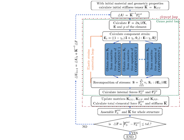
|
| Figure 31: Scheme of the generalized mixing theory formulation for finite strains implemented in PLCd for a total Lagrangian framework (reference configuration), based on the scheme of the hybrid formulation in Figure 6. The subindex indicates iteration number in the present load increment. The definition of each term is available in the notation list. |
As an example, the experimental data obtained by Martins et al. [86] is used to illustrate how the manifestly different behaviours of fibre and matrix can be represented by means of the damage model proposed, particularized for Ogden hyperelasticity, and in the framework of the generalized mixing theory.
The work by Martins et al. provides experimental stress-stretch curves obtained from an uniaxial tensile test of a rectus sheath sample in the longitudinal and transversal directions. Using Matlab's Curve Fitting Toolbox [108], an initial estimate of the material parameters of fibre and matrix were obtained, which were then manually adjusted in the numerical reproduction of the sample to better fit the experimental curve. The material parameters used are given in Figure 32, together with the stress-stretch curve numerically obtained using generalized mixing theory and the Ogden-based damage formulation implemented in PLCd [1]. In the sake of simplicity, the fibres were assumed to work completely in parallel, i.e., in the generalized mixing theory. Due to lack of information, the fibre contribution to the composite was estimated as 20% of the composite, based on information available in literature. A different proportion of fibre and matrix in the composite would obviously lead to a completely different stress response of the fibre in order to fit the composite response with the experimental data.
![Cauchy stress vs. stretch of the composite and its individual components modelled with the Ogden-based damage formulation and generalized mixing theory (χ=0) to reproduce the experimental data by Martins et al. [86] (left) and the material parameters used (right).](/wd/images/thumb/f/f0/Draft_Samper_593843246-Dam_comp.png/294px-Draft_Samper_593843246-Dam_comp.png)
| ||||||||||||||||||||||||||||||||||||
| (32) Cauchy stress vs. stretch of the composite and its individual components modelled with the Ogden-based damage formulation and generalized mixing theory () to reproduce the experimental data by Martins et al. [86] (left) and the material parameters used (right). | ||||||||||||||||||||||||||||||||||||
|
2.4.2 Tensile/compressive switch
Most fibred soft biological tissues consist of collagen fibres embedded in an isotropic ECM. The modelling assumption that fibres cannot support compression can be made in such case [109]. From a computational point of view, this requires “turning off” the fibre contribution to the model when this component of the composite is under compression. In the context of the generalized mixing theory, this requires affecting the compressive response of the simple material (the fibre, in this case). Thus, we propose introducing a tensile/compressive switch that affects a particular constitutive model of choice. Introducing an on/off switch is not a viable option because it generates computational instabilities in the case of complex stress states due to the sudden change in stress in a same Gauss point from one load step to the next. The fact that hybrid elements are being used does not contribute at all to the convergence of the problem.
Therefore, a smoothing function is introduced, which allows to transition from the purely tensile (full response) to the purely compressive (null response) of the fibre without a sudden discontinuity. In addition, the option to choose a reduction factor is also given, where means that the compressive response is reduced a 100% with respect to the tensile one, that is, the compressive response is null. Conversely, means that the compressive and tensile responses are exactly the same and, thus, no switch is applied. The function used to this aim is
|
|
(2.119) |
where is the slope of the function and is the stretch in the fibre direction. The effect of the two user-modifiable parameters and are graphically depicted in Figure 33.
![Role of the reduction factor r and slope value b, both modifiable by the user, in the tensile/compressive switch function implemented in PLCd [1].](/wd/images/thumb/9/90/Draft_Samper_593843246-Switch_func.png/360px-Draft_Samper_593843246-Switch_func.png)
|
| Figure 33: Role of the reduction factor and slope value , both modifiable by the user, in the tensile/compressive switch function implemented in PLCd [1]. |
Table 6 describes the scheme introduced at the Gauss point constitutive level to produce a smoothed tensile/compressive switch for a given simple constitutive equation in a TL framework. The algorithm requires the deformation gradient tensor , the second Piola-Kirchhoff tensor obtained by means of the chosen simple constitutive equation and the material parameter “switch direction” . This parameter is a unit vector defined by the user that indicates the direction in which the switch is to be applied. From a physical point of view, should correspond to the initial orientation of the fibres in the ECM. The scheme has been implemented solely for the TL framework, but extension to the pUL framework would only require replacing by .
| Algorithm at each load increment (applied after computing the stress at simple constitutive level)
User parameters: Reduction factor of the smoothing function , slope of the smoothing function and switch direction unit vector . |
| Given: deformation gradient tensor and second Piola-Kirchoff stress tensor .
Translate switch direction unit vector into present configuration, , and compute stretch in the present switch (fibre) direction as the norm of , . Calculate the value of the smoothing function for the value of computed above, . Affect the stress tensor with the smoothing function, . |
The tensile/compressive switch has been used in the uniaxial example with Ogden hyperelasticity (see Figure 14). Figure 34 shows the results obtained for a same slope of the smoothing function and different reduction factors. The switch manages to reduce the stress response in comparison to the original curve (solid yellow line). There is a transition zone from the tensile to the compressive response when the switch is activated. This is especially visible for the case with in which the compressive response at first has negative stress values which, as the compression progresses, are reduced to zero. The tensile part is also slightly affected by the transition zone in the initial stages of tensile loading, although the difference with the original curve is minimal. The span of this transition period is given by the chosen value . Higher values of will reduce the transition period but, of course, will also increase the numerical instability of the solution due to the abrupt change in material response. This is the case, especially, for complex geometries that will induce triaxial stress states in which there might not be a predominant tensile/compressive direction or this direction might shift considerably for a same Gauss point from one load step to the next. Thus, smaller load steps tend to improve the convergence of the solution.
In conclusion, the tensile/compressive switch is a tool that allows accounting for the fact that fibres in soft biological tissues have a different response in tensile loading than in compressive loading. However, the solution proposed has its limitations. The main one is that its robustness is linked to the span of the smoothing function and a trade-off between a small transition zone and a robust computation is required. In addition, the switch proposed here affects the whole stress tensor equally, that is, stresses in all directions of the fibre will be reduced the same percentage when the fibre is working in compression for the selected switch direction . Thus, the tensile/compressive switch proposed is only valid for quasi-uniaxial stress states. This, however, should not be a problem since the purpose of the switch is precisely to “deactivate” the fibre response in compression. Then, one would expect the user to set up in the fibre direction and to use this in conjunction with the generalized mixing theory described in the previous section. In this way, this problem is mitigated since the fibre should only contribute in the parallel direction, which would coincide with the switch direction.
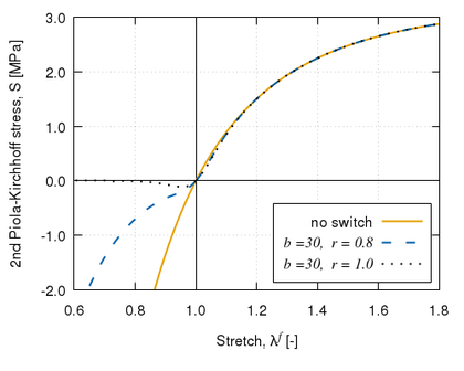
|
| Figure 34: Results for the tensile/compressive switch used in the Ogden example of Figure 14 to illustrate the effect of the reduction factor for a same value of the smoothing function slope . |
2.4.3 Anisotropy using space mapping
The anisotropy of soft fibred biological tissues is typically addressed through the definition of two separate strain energy density functions as described in 2.1. One accounts for the isotropic contribution of the matrix and the other, for the anisotropic contribution of the fibres. Then, the anisotropic specific strain energy density function must be specifically defined in terms of the pseudo-invariants of the fibre orientation vectors.
The usage of the generalized mixing theory described in section 2.4.1 to reproduce soft tissue behaviour allows considering any of these anisotropic specific strain energy density functions to describe the behaviour of the fibres in the the composite tissue. However, we propose using the approach introduced by Oller et al. [110,111,112], to model anisotropy in the simple material behaviour through space mapping. In this way, isotropic constitutive formulations can be used to describe anisotropic behaviour of simple materials.
The idea of using a mapped stress tensor to formulate the anisotropic behaviour of a material by means of an equivalent isotropic solid was first introduced by Betten [113] for creep modelling. It was then extended to the mapping of both stress and strain tensors by Oller et al. [110]. This concept is especially useful in that it profits of the advantages of the well-known isotropic models, namely, the analytic and computational techniques for isotropic constitutive equations.
The formulation [9] presented here is a means of generalizing any classic isotropic formulation, such as hyperelasticity or damage, to account for anisotropy. It is based on the translation of the material constitutive parameters and the stress and strain states from a real anisotropic space to a fictitious isotropic space. Once in the fictitious isotropic space, the isotropic constitutive models and associated procedures can be used to determine the material behaviour, which is then translated back into the real anisotropic space to obtain the anisotropic response of this material behaviour.
Through the use of space mapping, an anisotropic behaviour is represented with an isotropic formulation. Hence, an explicit mathematical expression of the model in an anisotropic form is not required. Instead, through a numerical transformation, an explicitly isotropic formulation can be converted into an implicitly anisotropic characterization of the material behaviour. All the material anisotropy information is contained in the fourth-order transformation tensors and , both defined in the reference configuration. In this manner, instead of computing the stresses in terms of the strains through an anisotropic constitutive equation (orange arrow in Figure 35), the strains are converted to the fictitious isotropic space through
|
|
(2.120) |
Then, the fictitious isotropic stresses are computed by means of an isotropic constitutive equation and, finally, these are converted back to the real anisotropic space through
|
|
(2.121) |
Here, the overline indicates the tensor belongs to the the fictitious isotropic space. The blue arrows in Figure 35 schematically depict this procedure.
This methodology was initially developed in the context of elastoplasticity to be able to use the well-known and thoroughly studied isotropic yield functions to describe anisotropic material behaviour without having to resort to explicit definitions of anisotropic yield criteria which do not always satisfy the invariance conditions [110]. In this context, the stress transformation tensor is
|
|
(2.122) |
where and are the second-order stress tensors representing the corresponding fictitious isotropic and real anisotropic strengths [9].
In the case being studied here, the original framework can be simplified because the purpose of the space mapping is to relate stiffnesses, not yield strengths. Hence, is considered. However, unlike the original set-up, the stress-strain relationship is highly nonlinear because hyperelastic formulations are being considered for the isotropic constitutive model in the fictitious space. Then, at a given increment of a loading process, the constitutive relation in the real and fictitious spaces can be reduced to and , respectively, where and are the pseudo-constitutive tensors for that particular load increment in the fictitious isotropic and real anisotropic spaces, respectively. Considering these relations and taking into account the definitions in 2.120 and 2.121, the transformation tensors are related through
|
|
(2.123) |
where the must be adequately defined such that the desired proportionality relation between and is obtained. For example, in the case of a transversally isotropic material in which the longitudial direction exhibits a higher stiffness than the transversal directions, the easiest definition of is a diagonal tensor with anisotropy ratios in the terms affecting the longitudinal direction. These anisotropy ratios indicate the additional amount of stiffness in the longitudinal direction with respect to the transversal ones.
2.5 Conclusions
The numerical modelling of the passive behaviour of soft biological tissue has been addressed by means of generalized mixing theory in conjunction with phenomenological hyperelastic and finite-strain damage models.
The numerical and thermodynamic bases of quasi-incompressible hyperelasticity have been reviewed and the most common hyperelastic models used in the characterization of soft tissues have been described. Then, the neo-Hookean and Ogden hyperelastic formulations have been developed in detail and implemented in the in-house FE code PLCd [1]. The neo-Hookean formulation does not manage to capture the characteristic J-shaped stress-stretch curve of soft tissue, but it may be useful in reproducing the ECM behaviour in the context of mixing theory. Ogden hyperelasticity manages to reproduce the highly non-linear response with agreeable accuracy. The computational problems derived from the use of the selected hybrid elements (Q1P0, Q2P0 and T2P0) have been pointed out and discussed.
Then, the thermodynamic bases of finite-strain damage have been reviewed and a generalized damage model has been proposed in order to provide a flexible and versatile formulation, capable of reproducing a wide range of tissue behaviour. To this aim, linear and exponential softening have been used in the model, which has been particularized for the neo-Hookean and Ogden formulations previously implemented in PLCd. Yet, the formulation developed can be easily adapted to any chosen hyperelastic model. Other softening laws could also be easily introduced, but the ones proposed require identifying only two material parameters, which can be determined experimentally, to characterize the behaviour of biological tissue. Again, computational problems that may arise due to the use of hybrid elements have been discussed.
Finally, the formulation of the generalized mixing theory has been briefly described and the use of a tensile/compressive switch and space mapping to account for anisotropic behaviour has been addressed.
To our best knowledge, the mixing theory approaches used up to date and available in literature for the modelling of soft tissue behaviour manage the contribution of each material component at the level of specific strain energy density function. Therefore, a closed formulation is produced which includes the contribution of the collagen fibres and ECM at constitutive level, usually oriented to reproducing a particular tissue's behaviour. The generalized mixing theory also manages the contribution of each material component at this same level but allows evaluating the interaction of the different constitutive models at a more general level, working as a “constitutive model manager” . It allows to separately represent each component behaviour (matrix and fibres) to obtain the overall composite behaviour (biological tissue). Used in conjunction with a series of phenomenological models capable of spanning a large scope of material behaviours, it is a powerful tool in achieving a general multi-purpose constitutive formulation for representing soft tissue behaviour.
We believe the generalized approach allows for more flexibility in composing the overall behaviour of the tissue since new constitutive models to represent fibre or matrix behaviour can be easily introduced if required. In addition, the constitutive models proposed to represent the simple constituent material behaviour have a solid and established thermodynamic basis, which allows for better tracing of the individual component's thermomechanical behaviour.
The generality of the formulation entails a certain loss of detail, namely, micro-structural phenomena that cannot be captured unless specific micro-mechanical constitutive models are introduced into the picture. The generalized mixing theory could replace the phenomenological constitutive model of a certain component for a mechanistic one if desired. Nonetheless, in pursuing a general constitutive formulation to represent the passive properties of soft biological tissues, one assumes that the representation of particular behaviours might not be as detailed and exact as if the formulation were specifically developed for that purpose or application.
3 Constitutive modelling of active properties
3.1 Background
A characteristic feature of living biological tissues is that they have the capacity of growing, adapting, remodelling and, in general, evolving in response to external loads and environmental stimuli. However, none of these processes take place solely due to the mechanical and environmental factors. There needs to be, in addition, the appropriate biological conditions.
Although the concepts of growth and remodelling are quite intuitive, let us establish the usage of these and other related terms considered in this particular work. The definitions given by Humphrey and Rajagopal [114] are employed as reference.
- Adaptation. Any acute or chronic change in the biological state, properties, mass or internal structure of a tissue in response to a change in the environment.
- Morphogenesis. Development of a fertilized egg into a mature organism. It is possible due to genetically programmed adaptive processes that involve changes in properties, mass and internal structure of a tissue.
- Homeostasis. Normal programmed adaptive processes that maintain a balanced turnover of cells and ECM without a net change in properties, mass or internal structure of a tissue 1.
- Ageing. Gradual changes in properties, mass or internal structure of a tissue following the maturity stage in the organism. It is independent of injury and disease, although they lead to a higher possibility of “natural” death.
- Healing. Adaptation process in response to injury or disease that involves changes in properties, mass or internal structure of a tissue. Its aim is to restore the original function, previous to the injury or disease, of the tissue or, if this is not possible, at least arrest the extent of damage.
These adaptation processes typically take place through a combination of the following phenomena:
- Growth. An increase in mass and volume, usually at constant density. This is achieved through an increase in number (proliferation, hyperplasia or migration) or size (hypertrophy) of cells 2, or through the synthesis of new ECM. Although growth may be associated with changes in the density or properties of the tissue, in this study growth will be assumed to occur at constant density.
- Atrophy. Inverse or negative growth, i.e., decrease in mass and volume. This typically occurs through cellular death (necrosis or apoptosis 3), cell migration or degradation of the ECM.
- Remodelling. A change in the internal structure of the tissue. This is achieved through the reorganization of the existing constituents or through the synthesis of new constituents that have a different organization to that of the existing ones. Remodelling may or may not change the density of the tissue, but it always changes material properties such as the stiffness of the tissue.
The first modern studies regarding living matter saw growth as a change in form [115,116] but there is now wide acceptance in the continuum mechanics community that it is change in mass that defines growth which, in turn, is related to changes in form. One of the driving forces behind this change in mass are the mechanical loads applied on the tissue. This phenomenon was first described in bone by Wolff in 1870 [117] but many researchers have contributed since to refine and develop the theory of functional adaptation of bone, being Frost [118] the most renowned.
The first application of the functional adaptivity in a continuum mechanics framework is credited to the theory of adaptive elasticity by Cowin and Hegedus [119]. Changes in mass are characterized by means of open-system thermodynamics, an approach used by many researchers up to date [120,121]. Another widely-accepted approach to modelling growth makes use of a multi-phase material and continuum theory of mixtures to represent changes in mass [114,122,123].
The former treatment of growth requires that the gain and loss of mass be translated into non-uniform changes in form. In fact, simplified models based on open-system thermodynamics typically characterize growth through non-linear kinematics by means of the change in volume associated with the change in mass. In mathematical terms, this is done through the decomposition of the deformation gradient tensor 4,
|
|
(3.1) |
where corresponds to the elastic part of the tensor and to the incompatible part, which includes the growth and remodelling effects.
This was explicitly written by Rodriguez et al. in 1994 [124], however, the concept of growth as an incompatible configuration had already been discussed before [125,126,127]. The elastic part of the deformation gradient defines the mechanical response of the tissue whilst the adaptation effects are modelled through the incompatible part which is controlled by the stress imbalance in the tissue. In particular, the stress imbalance, related to a homeostatic imbalance, activates growth in the tissue. The current configuration is then reached through an elastic deformation which ensures the compatibility of the deformations with the final growth. Figure 36 shows a schematic diagram of the relationships between the three configurations.
![Schematic representation of the multiplicative decomposition of the deformation gradient, inspired by [186]. Density, volume and mass relations in the different configurations are given for a continuum growth process at a given time. At the initial time, all configurations collapse into a single one. The definition of each term is available in the notation list.](/wd/images/thumb/9/9b/Draft_Samper_593843246-Configs.png/480px-Draft_Samper_593843246-Configs.png)
|
| Figure 36: Schematic representation of the multiplicative decomposition of the deformation gradient, inspired by [186]. Density, volume and mass relations in the different configurations are given for a continuum growth process at a given time. At the initial time, all configurations collapse into a single one. The definition of each term is available in the notation list. |
The intermediate growth configuration is incompatible and, thus, it is not a physical state attained by the tissue. Hence, the difficulty in defining the evolution equations for , which cannot be described through direct experimental observations. An aspect which has been questioned from this formulation is that, because mass is added to and lost from the tissue during the growth process, there no longer exists a fixed reference configuration when the mapping between configurations is defined only by the deformation [128]. However, there are several ways to overcome this issue, as described in Ambrosi et al. [129]. Other authors reject the multiplicative decomposition of growth because it focuses on the consequences of growth (changes in form) instead of on the biological processes which drive growth (cell and matrix turnover). This matter is addressed by some through micro-mechanical modelling of tissues, i.e., growth is based on cell-level micro-structure behaviour which can, to a certain extent, be characterized experimentally [130,131]. An important downside of this type of approach is that it requires defining the actual pathways by which mechanical and chemical activity of cells is translated into growth of tissues [129].
Despite these concerns, the focus in this study is in continuum modelling of growth and remodelling, which is a topic that has attracted the attention of the computational mechanics community over the past couple of decades. Articles by Ambrosi et al. [129], Menzel and Kuhl [132] and Kuhl [133] provide an excellent review on the different approaches used to deal with growth and remodelling, as well as the current challenges in this field of research.
Following this continuum approach to model growth, the issue is in specifying, on the one hand, the driving forces behind this phenomenon and, on the other, how the growth tensor evolves. With respect to the former, the main difficulty is in accounting for the biological stimuli, i.e., the effect of the tissue's metabolism, in addition to the mechanical stimulus that drives growth in living tissues [134,133]. Regarding the latter, finite growth has been typically categorized into volume, area and fibre growth [135,132,133]. These topics will be addressed in detail in section 3.2, as well as the development and implementation in the in-house FE code PLCd [1] of a growth model that takes into account the role of the metabolism. The model is first described for volumetric growth and then extended to include anisotropy. Volume growth is characterized by means of an isotropic tensor while the area and fibre growth models are described through anisotropic growth tensors. In this context, remodelling has often been understood in literature as an evolution or reorientation of the anisotropy direction in the tensor [132].
However, remodelling has been defined as a change in the internal structure of the tissue, a concept that includes much more than fibre reorientation. It may involve, for example, reorganization of the tissue constituents through synthesis and degradation. This has been tackled as a structural optimization problem in bone remodelling applications [129]. Also, remodelling is known to result in a change of tissue stiffness. This has been addressed in bone remodelling by Doblaré and García [136] through the formulation of a constitutive model in a CDM framework, in which the internal variable of the model is able to degrade (or regrade) with and without mass increase.
In soft tissue, remodelling is a key part of the healing process. The repair of soft tissues is known to be driven by a complex sequence of events involving cellular processes as well as biochemical and biomechanical factors [137,138]. The exact role of many of these factors is not completely understood yet. Nonetheless, from a physiological point of view, the healing process is classified into four distinct but overlapping phases:
Haemostasis The loss of structural integrity in the tissue immediately activates the coagulation cascade. Platelet aggregation and constriction of the injured vessels prevents further blood loss and a platelet-rich fibrin clot is formed. The activation of these platelets is associated with the secretion of several growth factors that initiate the healing process. Yet, this process is still not fully comprehended since healing is known to occur in wounds with no haemorrhage [139].
Inflammation As part of the organism's immune response, neutrophils infiltrate the site of injury within the first one to two days and start to phagocytose bacteria and debris to prevent infection of the wound. Within two to three days after injury, macrophages attracted to the wound site by chemoattractants have replaced the neutrophils. Macrophages further debride the wound and release cytokines, which stimulate angiogenesis and enhance the production of fibroblasts. After three days, lymphocytes appear in the site of injury and seem to play a role in regulating the proliferative phase through the production of ECM [140].
Proliferation Once the inflammatory response is balanced and the wound has been cleared of debris, the repair of the defect begins. This phase usually starts about three days after the injury and can last up to several weeks. Fibroblast proliferation and migration takes place, resulting in the synthesis and deposition of collagen to form the granulation tissue. Through angiogenesis, a vascular network of capillaries is formed that provides the necessary oxygen and nutrients in the healing tissue. The provisional ECM is highly disorganized and contains “flaws” such as fat cells and inflammatory pockets [137]. Skin wounds additionally exhibit epithelialization and wound retraction [141].
Remodelling The final stage lasts from weeks to years and consists in a continuous synthesis and degradation of collagen as the ECM is remodelled and the granulation tissue becomes the scar tissue. As this matrix turnover takes place, its composition shifts and reorganizes: the newly-formed blood vessels regress, the “flaws” are removed and the collagen fibres become increasingly organized [137]. Over time, and under adequate biochemical and biomechanical conditions, the remodelled tissue approaches the characteristics of the original undamaged tissue. However, the completely remodelled scar tissue often does not fully recover the characteristics of the uninjured tissue it replaces.
The mathematical modelling of wound healing has been widely addressed since the development of the first models in the 90s [142,143,144]. These models focus on the underlying cellular and biochemical mechanisms to define and simulate dermal wound contraction [145,146,147] and angiogenesis [148,149,150] from a continuum-based approach. The inflammation and proliferation phases have also been modelled using a discrete or a hybrid discrete/continuum approach [151,152,153] and, more recently, a systems-biology multi-scale and multi-field approach has been proposed [154]. The reader is referred to the work by Buganza Tepole and Kuhl [155] and Valero et al. [156] for a comprehensive review of mathematical and computational dermal wound healing models.
On the other hand, the remodelling phenomena in soft tissue has also been extensively addressed. In general, it is treated together with growth and not necessarily in the biological context of the tissue healing process described above [11,129,157,132]. Many of these models aim at characterizing collagen fibre reorientation through evolving structural tensors [158,159,160,161,162,163]. A different approach characterizes growth and remodelling as a continual turnover of tissue constituents by means of a constrained mixture theory [114,128,164,165], or, more recently, a mechanistic micro-structural theory [166].
Over the past years, advancements in the field resulted in sophisticated models with cellular [167,168] and molecular [169] processes being the driving forces of remodelling. In this sense, much effort is directed towards representing remodelling in vascular tissue [170,171,163,172], with a particular focus on the pathological remodelling observed in aortic aneurysm tissue [173,174,175]. The mathematical modelling of the inflammation, proliferation and remodelling phases in ligament tissue has also been addressed [176,177].
Numerous studies, both in animal models and in patients, have shown that mechanical loading has a significant impact on the speed and efficiency of healing [178,179,180,181]. However, the optimal loading regime remains unclear and the detailed mechanobiogical mechanisms involved are not fully understood. Computational approaches have been widely used in bone healing mechanobiological modelling to enable predictions of bone healing and improve the understanding of both mechanical and biological mechanisms at play [182,183]. In order to apply this approach to soft tissue healing, a continuum constitutive model that can represent both the changing soft tissue mechanics during healing and, also, the proposed biophysical stimuli for the cells involved is required.
In this sense, a constitutive model for homeostatic-driven turnover remodelling (HTR) in soft tissues is developed, formulated in accordance with CDM and in an open-system thermodynamics framework. The main internal variable is a recoverable effective damage, similar to the one proposed by Doblaré and García [136] for bone remodelling. The HTR model developed in section 3.3 describes the overall change in material behaviour at tissue level of healing/remodelling tissues. Analogous to the growth model described in section 3.2, healing is not only driven by mechanical loading, but also by biological stimuli. In particular, the underlying metabolism in healing tissues is represented by phenomenological parameters.
Although growth and healing are separate phenomena, they typically occur together as the former initiates the latter and they often interact with each other. Thus, the models described in sections 3.2 and 3.3 have been developed separately but with the ultimate intention of combining them to obtain a more general constitutive formulation to reproduce the active behaviour of soft biological tissues, as discussed in section 3.4.
(1) This is one of the most remarkable characteristics of living tissues and it acts at many levels in the organism, in addition to the tissue level described here. A living organism manages a host of incredibly complex interactions in order to maintain the internal balance and return, when required, systems to their normal functioning range.
(2) Cell proliferation refers to the increase in the amount of cells due to the creation of new cells through cell division. In the case of cell migration, the increase in the amount of cells of a tissue is due to cell movements, i.e., cells migrating into the tissue. Hyperplasia or hypergenesis is tissue growth resulting from cell proliferation while hypertrophy is tissue growth resulting from the enlargement of the cells composing the tissue.
(3) Necrosis is the pathological death of cells, caused by external factors such as infection or trauma. In contrast, apoptosis is the programmed and targeted death of cells in the organism.
(4) This is the preferred approach for continuum-mechanics-based constitutive models trying to capture the growth and remodelling phenomena in soft tissue since, in this case, the model is necessarily defined in a finite strain framework.
3.2 Growth
Growth/atrophy is a key phenomenon in the adaptation processes characteristic of living tissues. It has a fundamental role in pathologies such as cardiac hypertrophy 1, aneurysms 2 and hypertrophic scarring 3, among others. Some of the factors that regulate growth/atrophy are fundamentally mechanic. and represent, in general, a stimulus for the adaptation process. Hence, the importance of studying these phenomena in the framework of a formulation that allows estimating the stress and strain fields and their relation to said phenomena.
In this sense, the multiplicative split of the deformation gradient tensor introduced in 3.1 allows deriving a constitutive formulation for growth in a continuum mechanics framework. This development, based on open-system thermodynamics, will be described in section 3.2.1. To complete the characterization of the growth phenomenon, the evolution of the growth tensor must be defined, as will be seen in section 3.2.2. Although mechanical stimuli are often driving factors in tissue growth, the role of the metabolism cannot be neglected. Hence, the evolution of the isotropic stress-driven growth tensor that accounts for biological availability proposed by Bellomo et al. [184,185] is adapted and introduced into the in-house FE code PLCd [1]. The details of the derivation and numerical implementation will be discussed in sections 3.2.3 and 3.2.4. Finally, this growth model is extended to account for anisotropy in the direction of growth, detailed in section 3.2.5.
(1) Ventricular hypertrophy is the thickening or enlargement of the heart muscle (myocardium), which may be associated with a smaller heart chamber.
(2) An aneurysm is an abnormal localized dilatation or enlargement of a blood vessel. As it increases in size, the risk of rupture, which has a high death rate associated with it, also increases.
(3) A hypertrophic scar is a raised scar, in which the healed tissue (the scar) is characterized by an excessive amount of collagen.
3.2.1 Thermodynamic basis of continuum growth formulations
In a growing body, changes of mass must be accounted for by means of the balance of mass equation for open systems, which in local form and in the reference configuration is [132]
|
|
(3.2) |
where is the density, is a mass source and is an influx of mass, which for our purposes will be considered zero. Then, integrating the expression yields
|
|
(3.3) |
where is the density at the initial time in the reference configuration. During the growth process, there is a change in mass but the density remains constant. Then, the densities in the different configurations (see Figure 36) are related by means of the growth tensor and the deformation gradient through
|
|
(3.4) |
Considering these definitions, a mass change at constant density requires that
|
|
(3.5) |
Then, the evolution equation for the density in the reference configuration
|
|
(3.6) |
is deduced 1. Here, is the velocity growth gradient or rate of growth. Recalling the initial mass balance equation 3.2, and assuming there is no influx of mass, then the mass source results in
|
|
(3.7) |
which allows determining the source of mass directly from the evolution of the growth tensor . This approach has been widely used to characterize growth as mass increase in soft tissues in a continuum mechanics framework [186,187,133].
Now, the stresses in the tissue can be obtained from any elastic potential through 2.26, as described in detail in section 2.2.3,
|
|
(3.8) |
Here, is the second Piola-Kirchhoff stress in the reference configuration and is the right Cauchy-Green deformation tensor, which is directly related to the elastic deformation gradient through . To obtain the corresponding stresses in the intermediate incompatible configuration , a push-forward 2.5 is performed on with the corresponding space-transformation tensor ,
|
|
(3.9) |
The Kirchhoff stress and the Cauchy stress in the current configuration are also obtained by means of a push-forward on ,
|
|
(3.10) |
where the complete deformation gradient has been used, since it is the one that directly relates the reference and current configurations (see Figure 36).
Therefore, any of the hyperelastic constitutive models described in section 2.2.4 could be used as basis for this type of growth model. The hyperelastic model would represent the passive behaviour of the tissue, while the definition of the growth tensor would account for the active behaviour of the tissue.
The tangent constitutive tensor, required in the numerical implementation of any constitutive model, is obtained as in the corresponding hyperelastic constitutive model chosen, using the elastic part of the deformation gradient, since the FE problem is solved either in the reference or the current configuration, but never in the intermediate one.
(1) The detailed deduction of the evolution equation is as follows: .
3.2.2 Characterization of growth in soft tissue through the growth tensor evolution
To complete the growth model derived in the previous section, the growth tensor must be defined. Based on the microstructural type of growth observed in tissues, finite growth has been categorized into volume, area and fibre growth [135,132,133]. These can be driven either by biochemical factors such as nutrients, hormones or growth-factor, or by mechanical factors like stress, strain or stretch, or by a combination of both.
Volume growth The simplest form of finite growth is to consider an isotropic growth tensor of the form [188]
|
|
(3.11) |
where is the second-order identity tensor and is the growth multiplier. Then, the grown volume will be and the elastic gradient tensor,
|
|
(3.12) |
The evolution of the growth multiplier is then defined in terms of the chosen biochemical or mechanical factors considered for the particular tissues. For example, Ambrosi and Mollica [189] propose modelling growth of tumours by means of a nutrient-driven expression. They define a growth speed, a maximum volume growth towards which the multiplier converges over time and a nutrient threshold beyond which growth occurs. Himpel et al. [187] consider a stress-driven evolution of the multiplier, governed by a pressure variable, to model the growth of cardiovascular tissue. Similarly to the previous model, growth occurs when the pressure value is above a given threshold and its evolution depends on the growth speed, a shape parameter for the growth curve and the maximum growth volume allowed.
Area growth In transversely isotropic in-plane finite growth, there is no growth in the out-of-plane direction. This “no-growth” direction is characterized by the unit normal of the growth plane, . Then, the growth tensor is [190]
|
|
(3.13) |
where the growth multiplier can be interpreted as the grown surface area, . Since there is no growth outside the plane defined by , the volume growth is . Inverting the growth tensor, the elastic gradient tensor results in
|
|
(3.14) |
being the unit normal in the spatial configuration.
Again, the evolution of the growth multiplier can be computed in terms of biochemical and/or mechanical factors selected for particular applications. Papastavrou et al. [191] propose computing it in terms of the growth factor concentration to model growth in airway walls by means of an evolution equation analogous to the one proposed by Ambrosi and Mollica [189] in volumetric growth. However, they replace the nutrient concentration variable for a growth factor concentration that now drives growth, which is limited by a maximum area growth. A strain-driven evolution of the area growth used to model skin growth is put forth by Buganza Tepole et al. [190]. The expression used is similar to the one proposed by Himpel et al. [187] in volumetric growth. However, now growth is driven by a physiological area stretch once a certain threshold is surpassed. Its evolution depends on the growth speed, a shape parameter for the growth curve and the maximum growth area allowed.
Fibre growth In this case, finite growth takes place along a single (fibre) direction, determined by the unit normal , with no growth in the cross-fibre direction. The growth tensor is defined as [192]
|
|
(3.15) |
where the growth multiplier is directly the fibre lengthening or stretch, . In an analogous manner to area growth, because no growth takes place outside the fibre direction, the total amount of volume growth is . Then, the elastic gradient tensor is computed as
|
|
(3.16) |
Once more, either biochemical factors or mechanical factors, or both, are considered by different researchers for the definition of the growth multiplier evolution. A hormone-driven evolution of the growth multiplier similar to the nutrient-driven and growth-factor-driven expressions proposed for the volume and area growth, respectively, is used by Holland et al. [193] to define plant tissue longitudinal growth. In this model, hormone concentration triggers growth when its value exceeds a given threshold. Growth evolves differently depending on the growth speed and shape parameter selected, and is bounded from above by a maximum stem lengthening value. A stretch-driven evolution equation is proposed by Zollner et al. [194] for skeletal muscle applications, which is analogous to the one described in area growth. Yet, now, the driving variable is the longitudinal stretch, which is limited by a physiological stretch limit.
Hence, whichever growth tensor is chosen to characterize growth in a soft tissue, determining the growth multiplier evolution is key to a successful representation of the active properties of soft tissues. Many equations have been proposed by researchers in the field for this purpose, usually based, up to a certain extent, on the biological observations of particular tissues. However, as in the damage evolution law used to characterize the passive behaviour of soft tissue (see section 2.3.2), we seek now a general expression for the growth rate. Then, we propose following the concept first introduced by Oller and Bellomo [134,184], which defines a stress-driven growth rate, limited by the effect of the metabolism, which is characterized through a phenomenological parameter that represents the biological availability for growth in the tissue.
3.2.3 Growth evolution considering biological availability
Following Lubarda and Hoger [186], the isotropic growth tensor 3.11 is defined as
|
|
(3.17) |
where the growth rate is
|
|
(3.18) |
and the mass source, following 3.7, is
|
|
(3.19) |
Here, has been taken into account.
By analogy with the principal stretches, the growth multiplier is now denoted as growth stretch. Its value will be the unity when the deformations are purely elastic, smaller than one when there is atrophy in the tissue and larger than one for growth. The evolution rule proposed for the growth stretch is
|
|
(3.20) |
where the function determines the growth/atrophy rate and the function is related to the metabolic part of the growth phenomena.
The function that determines the growth/atrophy rate is exclusively dependent on mechanical stimuli, by means of the trace of the Cauchy stress tensor, . If there is an unlimited source of nutrients, the growth rate will not be limited by the metabolic part (that is, ) and, thus, it will be directly the function . Figure 37 shows the function used, whose mathematical expression is
|
|
(3.21) |
![Growth function g\left(Tr\left(σ\right)\right) due to mechanical stimulus proposed by Bellomo et al. [184]. Reproduced and adapted with permission. The definition of each term is available in the notation list.](/wd/images/thumb/1/11/Draft_Samper_593843246-GrowthFunction.png/480px-Draft_Samper_593843246-GrowthFunction.png)
|
| Figure 37: Growth function due to mechanical stimulus proposed by Bellomo et al. [184]. Reproduced and adapted with permission. The definition of each term is available in the notation list. |
The mechanical growth function is defined in terms of the following material parameters.
- and are the superior and inferior limits, respectively, of the homeostatic equilibrium. When the value of is larger than , growth in the tissue will begin. Conversely, when the value of is smaller than , atrophy starts. In between, the homeostatic equilibrium is maintained, i.e., new cells are solely generated to replace those that die.
- and are the slopes of the growth and atrophy rates, respectively.
- and are the growth and atrophy limits, respectively. The maximum possible growth stretch rate the tissue may have is determined by the maximum rate of mass production, . This maximum rate is expressed as the percentage of the original mass which can be produced by unit of time, therefore
(3.22) This yields the maximum growth stretch rate in terms of the maximum rate of mass production, . Operating in an analogous manner with the maximum rate of mass loss, , the maximum atrophy stretch rate is obtained as . In the numerical implementation, it will be more convenient to use the normalized values and .
Both the slopes and the growth/atrophy stretch rate limits have a biological basis in the cell division and collagen recruitment rates of the tissue being represented.
In this growth model, an external mechanical stimulus is the basic requirement for growth to occur, but the metabolism of the tissue must also allow it. Biological availability is understood here as the complete set of internal elements (proteins, enzymes, growth factors, etc.) necessary for growth to take place. These are the “nutrients” the tissue needs in order to grow in response to a mechanical stimulus.
A variable of biological availability for growth is defined. This variable represents the mass production the metabolism can sustain with the available nutrients at a given time and is defined as a percentage of the original mass,
|
|
(3.23) |
where is the initial volume and is the grown volume. It can also be defined in terms of the nutrients stored in the tissue,
|
|
(3.24) |
where and represents the nutrients introduced into the system. Thus, the biological availability variable is, in fact, a balance of the incorporated nutrients over time and those used to grow, both expressed in terms of mass production.
The nutrient function has been defined as an initial reserve and a value increasing over time with slope (see Figure 38). The value is dimensionless and represents the mass increment allowed by the nutrients, i.e., a value of indicates that the nutrients available in the system can generate an increase of mass in the tissue of with respect to its original mass.
![Nutrients available for growth in the tissue, defined through the function Ni, similar to the one proposed by Bellomo et al. [184]. The definition of each term is available in the notation list.](/wd/images/thumb/8/85/Draft_Samper_593843246-NutrientFunction.png/240px-Draft_Samper_593843246-NutrientFunction.png)
|
| Figure 38: Nutrients available for growth in the tissue, defined through the function , similar to the one proposed by Bellomo et al. [184]. The definition of each term is available in the notation list. |
Then, if the biological availability for growth is below the potential growth induced by a given mechanical stimulus, the actual growth of the tissue will be limited to the growth allowed by the biological availability. Conversely, if the biological availability allows for a larger growth than the potential growth induced by a certain mechanical stimulus, the real tissue growth will be limited by the mechanical factors.
Finally, the biological availability function introduced in the definition of the growth rate 3.20 is
|
|
(3.25) |
where the (volumetric) growth rate allowed by the nutrients is divided by the term to obtain the growth stretch rate allowed by the nutrients 1.
The model presented here and originally developed by Oller and Bellomo [134,184] in the framework of continuum mechanics can be grouped into the growth models based on concepts seen in large-strain plasticity [195]. Then, the hypotheses of the continuous medium are modified the least possible in order to treat growth in the material. In particular, the reference configuration is considered to evolve over time but it is identified as the same body, not as a superposition of a deformed ungrown body and a grown one 2.
The reference configuration used in the model is the original one only with regard to geometry since it is obtained as the pull-back of the grown (and elastically deformed) current configuration. Then, the mesh and volumes in the reference configuration are the same as the original ones but the rest of properties that depend on time, such as mass if there is growth, are not constant and will change over time. Since the volume in the reference configuration is constant but mass evolves with time, the density in the reference configuration will also change. This has already been summarized in Figure 36.
In a nutshell, the growth model is developed in the current configuration (in terms of the Cauchy stress) because experimental data is obtained in this configuration. However, the geometrical part of the model, namely, the deformation gradient tensor, relates the reference and current configurations. Then, density is maintained constant in the current configuration (where the model is defined) as mass grows, which is achieved by means of the intermediate incompatible configuration that arises from the split of the deformation gradient tensor. In addition, many numerical solvers such as PLCd [1] solve the equilibrium equations in the reference configuration. And, hence, the need of identifying these three configurations and knowing the role of each one in relation to the model used.
(1) This operation is based on 3.22, but here is and is .
(2) The reader is referred to Ambrosi et al. [129] for more information on the approaches used by different authors to treat this aspect of growth in a continuum mechanics framework.
3.2.4 A constitutive model for volumetric growth considering biological availability
The growth model described in the previous section has been implemented in a finite strain framework coupled to the isotropic quasi-incompressible Ogden hyperelasticity described in section 2.2.6. Similarly, to the damage model proposed in section 2.3.4, it could be particularized for any hyperelastic formulation desired. Table 7 shows the scheme of the formulation implemented. In the interest of simplicity, it was decided that the user introduce the biological availability parameters per element, not per Gauss point.
The trace of the Cauchy stress tensor has been calculated as
|
|
(3.26) |
where is the deviator part of the Cauchy stress tensor, which is null, is its volumetric part and is the averaged hydrostatic elemental pressure. This allows implementing the model in a TL framework but avoids the need to perform a push-forward on the second Piola-Kirchhoff stress to obtain the Cauchy stress and, then, compute its trace. It was deemed that this would introduce unnecessary numerical noise. In addition, the second Piola-Kirchhoff stress of the present iteration previous to including growth effects would have to be calculated, incrementing the overall calculation time. The stress obtained in the previous iteration could be used instead, but this also would have required considerable changes in the code. Therefore, 3.26 was considered the most effective way to obtain the trace of the Cauchy stress tensor given the circumstances.
Initialization at and
Algorithm at each load increment
|
Algorithm at each load increment (continued)
|
The main characteristics of the growth model implemented in PLCd [1] are presented here by means of two representative three-dimensional examples. A homogeneous state under uniaxial tension is reproduced in a single-element problem with the aim of illustrating the basic constitutive characteristics of the growth formulation and the role of the material parameters of the model. Then, a rectangular plate with a double notch at its centre and varying biological availability throughout the specimen is subjected to a tensile load in order to show how growth is affected by biological availability.
An 8-noded hexahedral element with a single pressure point (Q1P0) has been subjected to a displacement-driven pure tensile load applied in a single step and then has been left to grow without applying any additional loads for 40 steps, corresponding each step to a day. That is, the cubic element with 1cm length sides is subjected to a stretch of , which is then kept constant for 40 days (see Figure 8). The Ogden material parameters used are kPa, and , which correspond to a Neo-Hookean behaviour. A bulk modulus of Pa, used in the hybrid formulation as a penalizer, has been considered. The growth properties of the example used as basis are a homeostatic superior limit kPa, a growth slope and a normalized maximum rate of mass production .
First, a series of examples with the biological availability part of the model deactivated have been run for varying values of these three properties in order to understand the role of each property. Figure 39 shows how a lower value of the superior limit results in larger values of growth stretch, since growth initiates for lower values of the trace of the Cauchy stress tensor. The tensile load applied in the first step already generates a small amount of growth, therefore, the growth stretch is already larger than one in the first day of the simulation. Also, the decrease in the trace of the Cauchy stress tensor is inversely proportional to the increase in the growth stretch. Obviously, as mass (volume) is added to the element through growth, stress must necessarily decrease if there is no change in the applied load.
Figure 40 illustrates how the growth slope is directly related to the growth stretch rate and higher values of this slope result in a steeper growth stretch rate along time. In addition, the figure shows how, once the trace of the Cauchy stress tensor is below the homeostatic superior limit kPa, growth halts and the growth stretch value remains constant.
Finally, the effect of the maximum rate of mass production is depicted in Figure 41. Low values of mean that the growth is taking place at the constant value in Figure 37. This translates into a linear growth stretch rate instead of a non-linear one, as observed in Figure 41. The case shown in this figure is of special interest because growth takes place at the maximum rate of mass production for the first 20 days, approximately, but once the trace of the Cauchy stress tensor is below a certain value, the growth stretch rate becomes non-linear. This is because the decrease in the value of the trace means that the growth rate is no longer in the zone governed by , but has entered the zone of the function governed by (see Figure 37).
After studying the effect of the growth parameters on the numerical response, the biological availability part of the model has been activated to see how the nutrient function affects the response. Initially, three examples were run with a very high nutrient function, a moderate one and a very low one. Results are plotted in Figure 42. As expected, for a high nutrient function, the growth behaviour is identical to the result obtained when the biological availability was not activated (for example, in Figure 41). For a very low nutrient function, the biological availability is not enough to allow the growth of the element and, thus, the growth stretch and the trace of the Cauchy stress tensor remain constant along time. In an intermediate case, growth begins later than the case with full biological availability because growth cannot initiate until enough nutrients have been accumulated, and these are being accumulated at a lower rate than in the full biological availability case.
However, the nutrient function not only affects the moment when growth begins, but also the growth rate. This is observed in Figure 43. Note that the nutrient function is accumulative so, a function that is constant over time means that, once these nutrients have been spent, growth will completely halt, as observed in the figure for case and . Also, an initially higher reserve of nutrients (larger ) does not necessarily translate into growth initiating earlier in time. Growth will start when , therefore, it is the combination of and that will dictate the beginning of growth.
A tensile test has been performed on a larger specimen in order to assess the effect of an unequal distribution of biological availability. A rectangular 30mm20mm1mm specimen with a central double notch has been subjected to a displacement-driven pure tensile load. A stretch of is generated and then kept constant for 40 days (see Figure 44). The specimen has been meshed with 411 quadratic hexahedral elements with a single pressure point (Q2P0). The Ogden material parameters used are the same as in the previous example. The growth properties considered are kPa, and . A nutrient function with and has been defined for the right half of the specimen whilst the left half has been given a null nutrient function, i.e., no biological availability.
![Boundary conditions, prescribed displacements and reference elements of the double-notched specimen used [184]. Element A in blue, element B in green, element C in yellow and element D in red.](/wd/images/thumb/5/50/Draft_Samper_593843246-NotchBCs.png/180px-Draft_Samper_593843246-NotchBCs.png)
|
| Figure 44: Boundary conditions, prescribed displacements and reference elements of the double-notched specimen used [184]. Element A in blue, element B in green, element C in yellow and element D in red. |
Results show that the initial stress field is symmetric, since no growth has taken place yet. As time advances, the left part of the model, which has no biological availability, remains the same while the right part suffers growth and, thus a reduction of the trace of the Cauchy stress tensor (see Figure 45). The post-processor GiD [67] used to view the results allows smoothing of the elemental values, which results in the more accessible growth stretch and pressure distributions given in Figure 46. The evolution of the growth stretch and pressure distributions at the four elements marked in Figure 44 have been plotted over time in Figure 47. Elements A and D, and elements B and C begin with the same values but, over time, elements A and B do not grow due to lack of biological availability. The discrepancy in the initial values of elements A and D is explained by the fact that growth already starts in the initial increment, when tensile loading is applied, for element D. The slight increase of the trace of the Cauchy stress tensor in element B is attributable to a change in the element geometry due to its closeness to the growth zone.
|

|
|
|
|
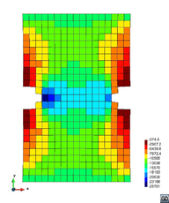
|
| Figure 45: Evolution of the growth stretch in the double-notched specimen at times , and (above) and the corresponding averaged pressure (below). Real deformation (1) is plotted. | ||

|
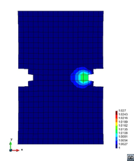
|
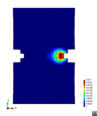
|
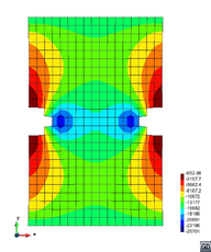
|
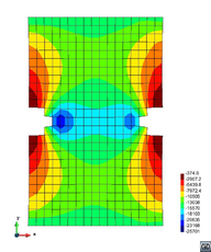
|
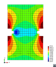
|
| Figure 46: Smoothed evolution of the growth stretch in the double-notched specimen at times , and (above) and the corresponding smoothed averaged pressure (below). Real deformation (1) is plotted. | ||

|
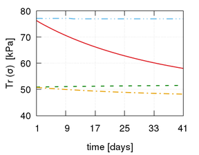
|
| Figure 47: Evolution of the growth stretch (left) and the trace of the Cauchy stress tensor (right) along time for the four elements marked in Figure 44. | |
3.2.5 Extension to anisotropic growth
In many cases, given the morphological characteristics of tissues, growth does not occur isotropically but following a direction that will depend on the tissue structure and the stress states acting on said tissue. To account for the directionality of this biomechanical process, the growth tensor in the constitutive model described in the previous section is extended to an orthotropic formulation [196].
Following the formulation by Goktepe et al. [197], the growth tensor in 3.17 is now defined as
|
|
(3.27) |
where , and are unit vectors, named structural vectors, that characterize the orthotropy directions in the reference configurations, and , and are the internal growth variables in the directions associated with the aforementioned vectors. As in the volumetric growth model, by analogy with the principal stretches, these variables are denoted as growth stretches. An evolution rule similar to the one used in volumetric growth (see 3.20) is proposed. However, it is now a second-order tensor given by
|
|
(3.28) |
where the tensor of growth stretch rates, , determines the growth in the different directions, establishing the orthotropy of the phenomenon. The growth stretch rates are limited by the maximum possible growth/atrophy stretch rates , a limit given by the maximum capacity of the tissue to generate new mass in ideal conditions. These are analogous to the growth and atrophy limits and , respectively, defined in the volumetric growth model. However, now different limits may be imposed in each growth direction depending on the particularities of the tissue being studied.
In general, the tensor is defined as a diagonal tensor such that the evolution of the growth stretches , and are uncoupled. The parameters that characterize each structural direction will depend on the structure of the tissue under study. In the most general case, they will be different in the three directions and, in the simplest one (volumetric growth), the three will be the same. The functions and in 3.28 remain the same as in the volumetric growth model. Hence, these functions are scalars that determine the magnitude of growth while the spatial distribution of the phenomenon is controlled by the terms in the second-order diagonal tensor .
As an example, this model is particularized for a transversally isotropic growth case to represent the growth of fibres in muscle tissue. In this case, the fibres in the tissue are known to increase their transversal section without appreciable changes in their length. Considering the direction of the fibre in the reference configuration is given by the structural vector , the growth stretches are
|
|
(3.29) |
Then, the growth tensor is
|
|
(3.30) |
where and represent now the growth stretches in the two directions orthogonal to the fibre direction. Assuming that growth is homogeneous in the transversal section of the fibre produces , where represents the growth stretch in the direction perpendicular to the fibre. Consequently, the growth tensor is reduced to
|
|
(3.31) |
Since there is a single growth internal variable, the transversal growth stretch , the growth stretch rate is reduced to the scalar
|
|
(3.32) |
where the function is given by
|
|
(3.33) |
In this way, the maximum growth rate is delimited by the maximum rate of mass production. The limit functions for growth and atrophy rate are denoted as and , respectively. The expression for the mechanical stimulus function has been given in 3.21 and the function quantifying the biological availability defined in 3.25 is now
|
|
(3.34) |
since the growth occurs now along a surface (two dimensions), not a volume (three dimensions).
A simple example is presented to verify and illustrate the behaviour of the transversal growth model described here. In a very simplified way, growth is seen to be controlled directly by the stress states in this example. Muscular growth is, in fact, associated with damage repair and inflammation in the muscle and it is this damage that depends on the stress states. In addition, the metabolic effect derived from the inflammation in the muscular fibres is also associated with growth. Given the complexity of this phenomenon, a simplified approach has been considered, where the growth stimulus has been directly linked to the stress state through the trace of the Cauchy stress tensor in the intermediate configuration.
A patch of tissue is numerically reproduced and subjected to displacement-driven tensile loading along the longitudinal axis. The initial geometry and deformations induced by the loading imposed are shown in Figure 48. The displacement induced is approximately 15% of the initial length of the specimen. A Yeoh hyperelastic model is used to characterize the passive part of the material's behaviour, with kPa, kPa and kPa [198]. These parameters correspond to the media layer in a coronary artery, which constitutes a compact elastic laminar tissue mainly composed of smooth muscular cells. Hence, it seems reasonable to assume transversally isotropic growth for this type of tissue.
The loading imposed on the tissue is maintained and the deformed specimen is left to grow for 30 days, considering a normalized maximum rate of mass production of per day. The biological availability is computed in terms of the initial nutrient reserve and an increasing value over time with slope per day. A superior limit of the homeostatic equilibrium kPa is assumed.
The evolution of the transversal growth stretch and the trace of the Cauchy stress tensor is shown in Figure 49. The imposed displacements generate a stress state at the initial time in the specimen such that the growth threshold is surpassed. Therefore, the tissue suffers a stress imbalance with respect to the homeostatic equilibrium and a mechanical stimulus for growth is generated. Growth evolves, limited by the metabolism's biological availability, producing an increment in the transversal section. Consequently, and because the loading remains constant, stress values in the specimen diminish over time.
3.2.6 Discussion
The growth model proposed in section presents some numerical issues, related to the elements chosen to solve the FE problem. The trace of the Cauchy stress tensor has been calculated as , where is the averaged pressure of the element. This pressure is obtained by adding the averaged nodal pressures of the element and dividing by the number of nodes. The averaged nodal pressure is, in turn, obtained by adding the pressure of the elements which contain that node and dividing by the number of contributing elements. The aim of this procedure is to obtain a smoothed distribution of the elemental pressure instead of the one calculated by the solver. In quadratic Q2P0 elements, not much difference is observed between the averaged and the normal distribution, but when linear Q1P0 elements are used, the difference is substantial, as observed in Figure 50. In fact, calculating the trace from the real distribution of pressure instead of , results in non-convergence for certain problems such as the tensile test on the double-notched specimen described in section 3.2.4.
This is most probably due to the checker-boarding of the pressure, clearly visible in Figure 50 (below left). As has already been noted in section 2.2.2, Q1P0 elements do not satisfy the inf-sup condition and are only known to work acceptably well for fine meshes, which is not the case in the example used. The use of the averaged pressure distribution overcomes the problems derived from these inaccuracies and results in growth stretch and averaged pressure values comparable to the quadratic case (see Figure 51, in comparison with Figure 47). Note, however, the pressure instability in the last steps of the linear model for element D. Obviously, the stress distribution in the specimen with linear elements will exhibit checker-boarding when the hydrostatic part of the stresses are obtained from the elemental pressure, not from the averaged pressure distribution. So, the growth model has been made robust in this manner, but the user must assess if the results obtained, especially in terms of stresses, are valid or not for the purpose being sought.
An alternative which is foreseeably more robust than using the averaged pressure distribution to compute the trace of the Cauchy stress tensor is to use the values from the previous converged step. Since pressure oscillates from one iteration to the next of the same load step until it converges to a certain value, using the last converged value of the pressure would probably result in faster convergence of the growth model. The problem is then that the growth will be based on the stress values of the previous step, instead of the present step. Thus, the use of this solution would only be acceptable for relatively small load steps.
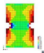
|
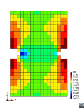
|
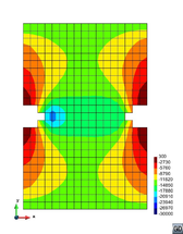
|
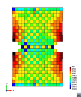
|
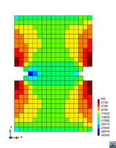
|
![Element pressure computed by the solver p (left), averaged pressure distribution pav used to compute Tr\left(σ\right) without (centre) and with (right) application of the GiD smoothing [67], for the last step in the double-notched specimen meshed with Q2P0 elements (above) and Q1P0 elements (below). Real deformation (×1) is plotted.](/wd/images/thumb/0/05/Draft_Samper_593843246-probL_PSmoothSv_41.png/168px-Draft_Samper_593843246-probL_PSmoothSv_41.png)
|
| Figure 50: Element pressure computed by the solver (left), averaged pressure distribution used to compute without (centre) and with (right) application of the GiD smoothing [67], for the last step in the double-notched specimen meshed with Q2P0 elements (above) and Q1P0 elements (below). Real deformation (1) is plotted. | ||
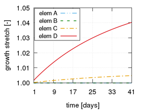
|
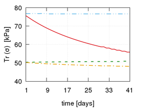
|
| Figure 51: Evolution of the growth stretch (left) and the trace of the Cauchy stress tensor (right) along time for the four elements marked in Figure 44, using Q1P0 elements instead of Q2P0 ones as in Figure 47. | |
3.3 Healing
A complex sequence of events drives the change in the internal structure of remodelling soft tissue. Remodelling is observed both in the final stage of the healing process leading to scar formation, and in the pathological remodelling of diseased tissues such as aortic aneurysm tissue. From a phenomenological standpoint, remodelling results, amongst other observations, in a tendency to recover or repair the injured ECM, with the tissue's stiffness tending to the original uninjured tissue stiffness.
A constitutive model for homeostatic-driven turnover remodelling (HTR) in soft tissues is proposed to account for this stiffness recovery. It is developed within the framework of CDM and is based on the thermodynamics of irreversible processes with internal state variables [71,69,68,72].
Unlike inert materials, tissues have an underlying metabolism, which is essential to the growth, healing and remodelling processes characteristic of living organisms. From a continuum mechanics standpoint, this metabolism introduces energy into the system, allowing for the “recovery” of the energy dissipated during damage and, thus, permitting a “reversal” of the damage produced in the material. Consequently, the total specific Helmholtz free energy density introduced into the system is the sum of the initial specific strain energy density function contained in the tissue and the specific strain energy density function introduced by the metabolism such that
|
|
(3.35) |
Here, the energies are given with respect to the density in the reference configuration and the tilde indicates the deviatoric or volume-preserving part of the free energy. The sub-index vol refers to the volumetric part.
The recovery energy reverses the damage in the tissue such that the internal damage variable is no longer accumulative in nature, i.e., as in classic CDM models. Specifically, we postulate the deviatoric part of the specific Helmholtz free energy density to be of the form
|
|
(3.36) |
where is the original (undamaged) hyperelastic specific Helmholtz free energy density given in terms of the deviatoric part of the right Cauchy-Green strain tensor, . The effective damage is the internal (recoverable) damage variable, which only affects the deviatoric part of the tissue's strain energy. Its rate is given by
|
|
(3.37) |
where is the rate of , an explicit Kachanov-like mechanical damage variable, and is the rate of , the repair or healing term. From a CDM point of view, may be associated to the micro-voids and small fissures that appear and extend as damage initiates and evolves. corresponds to a compact material with no voids or fissures whilst is a completely damaged material whose amount of voids and fissures is such that it can no longer carry any load. The healing term represents the reversal or “filling” of these micro-voids and small fissures such that the original load-carrying capacity of the material is recovered.
Then, corresponds to a mass deposition equivalent to the original undamaged material stiffness and, thus, coincides with a recovery energy , i.e., the initial pre-injury strain energy. Hence, the healing term can be defined in terms of the specific strain energy densities as .
Ideally, the original properties of the uninjured tissue should be recovered at the end of the healing process such that the healed tissue is indistinguishable from the pre-injured tissue. In practice, some healed tissues are softer than their corresponding healthy uninjured tissue [199,137,200] while others become stiffer, often loosing functionality. The latter is the case of fibrotic scar tissue [201,202,203], which has been associated with pathological conditions caused by an aberrant ECM production that results from perturbed homeostasis in the tissue [204]. In this work, the former case will be addressed and, thus, is assumed, i.e., at most, the original properties can be recovered. The full recovery () corresponds to a successful restoration of the tissue's homeostatic state.
The evolution of both and will be defined in more detail in section 3.3.2. However, since will be seen to implicitly depend on the tissue damage, it is anticipated that .
3.3.1 Thermodynamic basis of the reverse-damage healing formulation
The Clausius-Duhem inequality in terms of specific free energy density, considering the simplifying arguments introduced by Simo [88], is , where is the second Piola-Kirchhoff stress tensor. This expression, deduced in the framework of classic CDM, does not account for the energy introduced into the system to allow for the reversal of damage. To account for the entropy entering the system, a term analogous to the one described in the free-energy-based Clausius-Duhem inequality for open systems proposed by Kuhl and Steinmann [121] is added, resulting in
|
|
(3.38) |
Here, is the density of entropy source and is the absolute temperature. We assume the entropy is introduced into the system exclusively through an internal source, the system's metabolism. Hence, the entropy flux defined by Kuhl and Steinmann [121] is null here.
Introducing now 3.35 and 3.36, and considering that the inequality must hold true for any strain increment, leads to the constitutive equation
|
|
(3.39) |
Thereby, the following dissipation inequality must be satisfied
|
|
(3.40) |
An entropy source of the type typically found in the context of biomechanics [121] is considered, , with a normalized mass source . Here, is the healing rate introduced in 3.37, i.e., the normalized rate at which strain energy is introduced into the system to allow for damage reversal. Then, the dissipation inequality 3.40 becomes
|
|
(3.41) |
Introducing 3.37, this expression is reduced to the classic mechanical dissipation due to damage, given in the reference configuration, , which must be non-negative at any time.
3.3.2 Effective damage evolution
Following CDM theory, the stress level determines the damage in the tissue. The linear and exponential softening laws used in the generalized damage model described in section 2.3.3 are considered for the evolution of the variable ,
|
|
(3.42) |
Here, the initial damage threshold and the fracture energy are material properties per unit spatial volume that can be identified from passive in vitro tests and denotes the Simo and Ju energetic norm [69].
The evolution of the repair or healing variable is defined in accordance with the biochemical and biomechanical observations of healing soft tissue. It is inferred from the description of the phases of the healing process that damage is a trigger of this process, but healing only occurs when the metabolism allows for it (see Figure 52). Also, in many cases, the mechanical properties of the completely healed tissue remain inferior to uninjured tissue [199,137,200]. Based on this experimental evidence, the healing rate
|
|
(3.43) |
is proposed. Here, represents the Macaulay brackets [104], is a function that regulates how fast healing occurs (introduces a time scale) and defines the percentage of stiffness that is not recovered at the end of the healing process. Note the implicit character of the healing rate, since is a function of . In addition, because is also a function of , the healing rate is also implicitly dependent on the mechanical loading of the tissue.
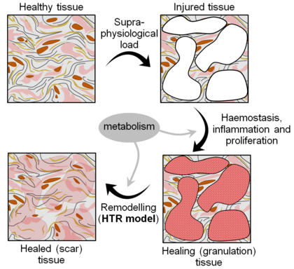
|
| Figure 52: Interpretation of the healing process in a CDM framework and contribution of the HTR model in this context. |
The irreversible stiffness loss parameter is a given value that dictates the amount of stiffness lost, with respect to the uninjured tissue's stiffness, at the end of the healing process. In other words, establishes the remanent effective damage that is not recovered in the completely healed tissue. For example, indicates that, after complete healing, the tissue will have recovered an 80% of its original stiffness, namely, there will remain a .
The function regulates the healing speed, which is directly related to the system's metabolism or biological availability. Here, the biological availability is understood as the complete set of internal biochemical elements (proteins, enzymes, growth factors, etc.) necessary for healing to take place [184]. Due to lack of experimental data and in the sake of simplicity, a constant healing rate has been defined, . The healing rate parameter is a given value that determines the healing time scale and is measured in .
Thus, the healing rate function proposed here complies with the basic biomechanical conditions that under absence of injury () or in case of no biological availability (days) healing will not occur.
3.3.3 The homeostatic-driven turnover remodelling constitutive model
The proposed HTR constitutive model has been implemented in PLCd [1], particularized for an Ogden hyperelastic model (see section 2.2.6). Details regarding the numerical implementation are schematized in Table 9.
Initialization at and
Algorithm at each load increment
(continue in the next table) |
| Algorithm at each load increment (continued) |
The corresponding tangent constitutive tensor is obtained as in 2.78, with the volumetric part of the tensor remaining the same, but the deviatoric part being now
|
|
(3.44) |
Here, corresponds to the material elasticity tensor of the undamaged material, , and the derivative of is
|
|
(3.45) |
Rearranging terms and isolating the derivative of , yields
|
|
(3.46) |
Now, considering the Simo and Ju criterion [69] as the energetic norm, , produces
|
|
(3.47) |
Introducing this expression into 3.46 and, then, into 3.44 results in
|
|
(3.48) |
The derivative of the mechanical damage variable with respect to for the linear and exponential softening laws 3.42 considered is derived in section 2.3.3 as
|
|
(3.49) |
The derivative of the healing variable with respect to , taking into account the healing rate defined in 3.43, is given by
|
|
(3.50) |
where denotes the present time. The Leibniz integral rule allows introducing the derivative into the integral and, eliminating the Macaulay brackets, the expression results in
|
|
(3.51) |
The numerical implementation detailed in Table 9 introduces an auxiliary mechanical damage variable, , to be able to detect the cases in which there is an (elastic) unloading on the tissue. This is due to the fact that the mechanical damage variable is updated at the end of each increment with the computed effective damage value () so that at the end of the healing process, when is recovered, there is no stored history of accumulated mechanical damage. This is in accordance with the definition of the HTR model's internal variable 3.37 in terms of rates.
It becomes clear from the numerical algorithm that the computed value of may decrease only when there is active healing, which occurs for . Hence, this variable is automatically bounded from below by , being 0 the lowest possible value that the effective damage may take. Since (as defined in 3.43) and the mechanical damage rate is necessarily non-negative (as deduced from 3.41), only increases when the mechanical damage progresses () which, at most, will produce a value . As a result, is automatically bounded from above by 1. Although is not required because is computed in terms of the implicit function defined for the healing rate , it could be calculated at the end of each load increment as and, considering the aforementioned bounds of and , it would be seen to satisfy .
The main characteristics of the HTR model are illustrated by means of a simple uniaxial tensile test example. Then, data on ligament healing taken from the literature is used to validate the model. Finally, an abdominal aortic aneurysm (AAA) [205] is numerically reproduced under different healing conditions to demonstrate the applicability of the model in reproducing experimental set-ups and the capability of the formulation to analyse geometrically complex models.
An 8-noded cubic element with cm length sides is subjected to a displacement-driven pure tensile load applied in steps of mm, as shown in Figure 8. Each load step corresponds to a time increment of 0.05 days. Two sets of hyperelastic and damage material properties have been considered (listed in Table 11), one reproduces a Neo-Hookean-like behaviour and the other, an Ogden-like one. A penalizer value times the maximum value of the shear moduli has been considered for the bulk modulus in all cases.
Ogden material behaviour Neo-Hookean material behaviour
| Parameter | Value |
| Parameter | Value |
In the first set of examples (see Figure 53), an irreversible stiffness loss parameter has been used, such that the initial stiffness properties will be completely recovered by healing. The healing rate parameter changed between days and days. A high healing rate ( days in Figure 53) is undistinguishable from the hyperelastic model because healing immediately compensates for the damage produced. This can be understood as a representation of the continuous turnover known to occur in living tissues. Also, a null healing rate ( days in Figure 53) results in a passive damage response, i.e. accumulation of damage in an inert material.
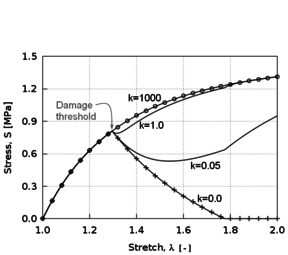
|
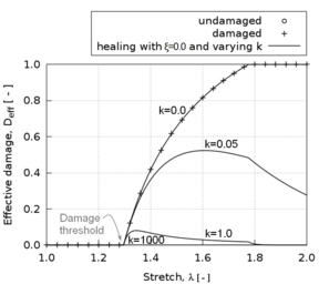
|
| Figure 53: Second Piola-Kirchhoff stress vs. stretch (left) and effective damage vs. stretch (right) responses of the homogeneous uniaxial tensile test example using the Neo-Hookean material parameters (see Table 11) with linear damage for an irreversible stiffness loss parameter and varying values of the healing rate parameter (values given in days). | |
The next set of examples (see Figure 54) shows the effect of varying the parameter , which dictates the final effective damage in the completely healed tissue. As expected, for a value , a behaviour analogous to the passive damage model is obtained since no stiffness can be recovered and damage continuously accumulates.
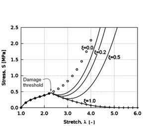
|
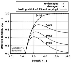
|
| Figure 54: Second Piola-Kirchhoff stress vs. stretch (left) and effective damage vs. stretch (right) responses of the homogeneous uniaxial tensile test example using the Ogden material parameters (see Table 11) with exponential damage for a healing rate parameter days and varying values of the irreversible stiffness loss parameter . | |
Finally, a loading-unloading-reloading case is reproduced for different values of the healing variables (see Figure 55) to illustrate how healing may continue whilst unloading takes place, such that damage progression and recovery (healing) may or may not occur simultaneously.
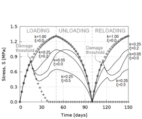
|
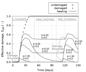
|
| Figure 55: Second Piola-Kirchhoff stress vs. time (left) and effective damage vs. time (right) responses of the homogeneous uniaxial tensile loading-unloading-reloading test example using the Neo-Hookean material parameters (see Table 11) with linear damage for varying values of the healing rate parameter (values given in days) and irreversible stiffness loss parameter . | |
Quantitative experimental data on healing is difficult to find in literature and, when available, is not always in a form which can be readily used and reproduced to validate numerical models. As one of the rare examples, the experimental work by Abramowitch et al. [207] on healing medial collateral ligaments (MCL) in goat knees provides excellent data to validate the HTR model. In their experiments, the MCL is surgically sectioned and the free ends of the ligament are realigned but not sutured, leaving a gap of about cm between the free ends [207,208]. The wound is then closed and the animals are allowed to recover for 6 weeks, after which they are humanely euthanized and their knees are prepared for testing. Typical tensile stress-strain curves are provided for the healed ligament and a healthy (uninjured) ligament used as control (see grey lines in Figure 56). Since there is no specific geometry and boundary conditions associated with these curves, the data has been used to calibrate material properties with the cubic element of the previous set of examples (see Figure 8). However, the length of the element sides has been reduced to cm to match the experimental data provided.
An uniaxial tensile loading is reproduced in order to estimate the Ogden and damage material properties which fit best the healthy stress-strain curve. These material properties are then used in a simulation with a forced initial damage , in which no load is applied but healing is allowed to progress for 6 weeks. An irreversible stiffness loss parameter has been considered since MCL scar tissue is known to regain at most % of its normal stiffness [199]. The healing rate parameter is adjusted such that, after a 6-week healing period, the stress-strain curve obtained for uniaxial tensile loading fits the experimental data. Table 12 summarizes the material parameters used in this numerical example and Figure 56 compares the numerical results to the experimental data. The set of parameters used was achieved by a manual trial and error approach and is not unique nor satisfies the minimum of an objective function. A penalizer value Pa has been considered as the bulk modulus.
| Parameter | Value |
| MPa | |
| MPa | |
| MPa | |
| Parameter | Value |
| kPa | |
| N/mm | |
| days | |
|
|
![Cauchy stress vs. engineering strain responses to uniaxial loading of a healthy and a 6-week healed MCL tissue following a surgical sectioning. FE results (solid black lines) were obtained using the material properties given in Table 12. The grey curves illustrate the response from the experimental data in Abramowitch et al. [207].](/wd/images/thumb/e/eb/Draft_Samper_593843246-Abramowitch.png/330px-Draft_Samper_593843246-Abramowitch.png)
|
| Figure 56: Cauchy stress vs. engineering strain responses to uniaxial loading of a healthy and a 6-week healed MCL tissue following a surgical sectioning. FE results (solid black lines) were obtained using the material properties given in Table 12. The grey curves illustrate the response from the experimental data in Abramowitch et al. [207]. |
An AAA is a permanent localized dilatation of the abdominal aorta which, if left untreated, progresses over time and can eventually rupture, leading to death. AAA rupture is a multi-factorial process that involves interacting biomechanical, biochemical, cellular and proteolytic aspects. In the latter stages of AAA disease, an irreversible remodelling is known to occur in the aortic wall connective tissue. This pathological remodelling is characterized by a progressive imbalance between the synthesis and degradation of collagen and elastin in the ECM. This degradation is linked to a decreased load-bearing capacity of the wall tissue, which leads to arterial dilatation. The reader is referred to [209,210,211] and references therein for further details on the many factors involved in the progression and rupture of AAAs.
The proteolytic degradation of structural proteins above may be regarded, from a macroscopic point of view, as a degradation of the tissue's properties. Thus, the HTR model has the potential to characterize this particular factor in the complex evolution of AAAs, linking the pathological arterial dilatation and its subsequent rupture to the healing capacity of the tissue.
A three-dimensional reconstruction of an AAA was obtained through segmentation of computer-tomography images (A4research, VASCOPS GmbH) [212] and meshed using 4707 hexahedral Q1P0 elements. A single element was included across the wall thickness with an approximately constant value of mm throughout the aneurysm. Therefore, bending effects are neglected in the simulation. The model is fully-fixed at the top slice and allowed vertical displacements at the bottom one. A blood pressure of mmHg (kPa) is applied in 200 load increments on the inner surface of the wall by means of a deformation-dependent follower pressure load on the face of each element. Material properties were estimated from the experimental tensile test data available in Gasser [31] using a single element (see Figure 8). A penalizer value Pa has been considered as the bulk modulus. The set of parameters used (listed in Table 13) was achieved by a manual trial and error approach and is not unique nor satisfies the minimum of an objective function. The corresponding constitutive response is plotted in Figure 57. The distal and proximal extents of the aneurysm are excluded from damage evolution, i.e. assigned the purely hyperelastic response shown in this same figure.
| Parameter | Value |
| kPa | |
| kPa | |
| kPa | |
| Parameter | Value |
| Pa | |
| N/m
|
![First Piola-Kirchhoff stress vs. stretch responses to uniaxial loading of an AAA tissue. The FE results (black lines) were obtained using the material properties given in Table 13. The grey dots illustrate the response from the experimental data provided in Gasser [31].](/wd/images/thumb/5/52/Draft_Samper_593843246-Gasser_2.png/390px-Draft_Samper_593843246-Gasser_2.png)
|
| Figure 57: First Piola-Kirchhoff stress vs. stretch responses to uniaxial loading of an AAA tissue. The FE results (black lines) were obtained using the material properties given in Table 13. The grey dots illustrate the response from the experimental data provided in Gasser [31]. |
The example was studied with two different values of the healing rate parameter and an irreversible stiffness loss parameter was assumed in both cases. Under non-pathological conditions, the aortic wall is continuously remodelling and, thus, for a high healing rate its behaviour should be that of a healthy tissue. Figure 58 shows the deformed shape of the same AAA at identical loading and boundary conditions but considering two different healing rate parameters: years (high rate) and years (low rate). The high healing rate resulted in deformations comparable to a sole hyperelastic simulation since damage is healed quasi simultaneously. However, for the low healing rate, the simulation failed at a blood pressure of mmHg (kPa). At this loading value, a high damage concentration localizes in a narrow band of elements (see Figure 59), which leads to structural instability and numerical failure in the following load step.
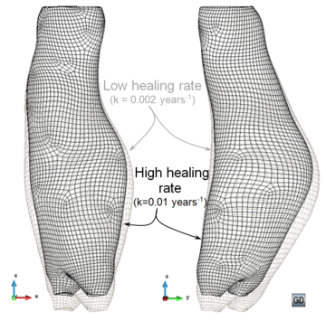
|
| Figure 58: Deformed shape of an AAA considering the material properties given in Table 13 and subjected to a blood pressure of mmHg (kPa). Two different healing rate parameters have been considered in addition to an irreversible stiffness loss parameter . The distal and proximal extents were excluded from damage and assigned a hyperelastic material behaviour. Real deformation (1) is plotted. |
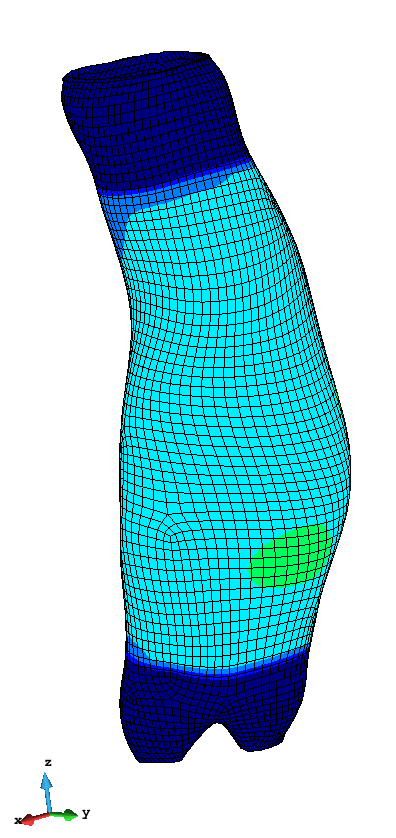
|
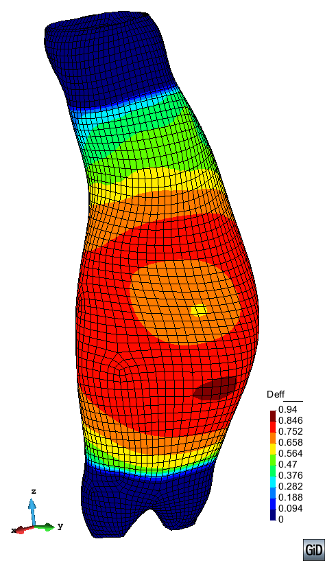
|
| Figure 59: Effective damage distribution in an AAA considering the material properties given in Table 13 and subjected to a blood pressure of mmHg (kPa). Two different healing rate parameters have been considered in addition to an irreversible stiffness loss parameter . The distal and proximal extents were excluded from damage and assigned a hyperelastic material behaviour. Real deformation (1) is plotted. | |
3.3.4 Discussion
The effective damage 3.37 drives healing in the HTR model. This variable is a direct representation of the tissue's state since it dictates the stiffness of the healing tissue, which can be measured through experimental tests. In contrast with previous remodelling models (see section 3.1), the present description does not attempt to capture the realignment of collagen or the processes taking place at cellular or microscopic level. Instead, it is a phenomenological model which aims to describe the overall change in material behaviour (stiffness) at tissue level of healing tissue.
The driving internal variable accounts for both mechanical and biological stimuli. Mechanical loading induces damage in the tissue as is a function of the stress. The injury produces a biological response such that, if the metabolism allows for it, healing occurs and the effective damage in the tissue is reversed (see Figure 52). The metabolism's action is quantified through the two healing parameters, and . Then, a healed tissue that has completely recovered the original properties is undistinguishable from the original tissue. The model is able to capture this, as seen in Figure 55 for the uniaxial tensile loading-unloading-reloading case with days;, where the reloading curve is exactly the same as the first loading curve.
In contrast, when the healed tissue does not recover the original properties (), it is assumed to have a remanent damage such that it is permanently softer than the initial pre-injured tissue. This is observed in Figure 55 for the cases with days; and days;. In both cases the reloading curves have a lower stiffness in their initial elastic portion than the corresponding portion in the loading curves. Note how a healed scar tissue that suffers additional injury will heal back to the first scar tissue properties, i.e., the stiffness loss is not accumulative over successive injuries in a same tissue.
The issue arises, then, whether this (new) healed material should maintain the updated damage threshold corresponding to the remanent damage value. An alternative would be to redefine the healed tissue as a completely new material by eliminating the remanent damage and affecting the hyperelastic (and, possibly, the damage) material properties instead. Then, the same effect would be achieved (lower stiffness), but the material would be considered simply as new and “undamaged”. In this case, if , an additional injury would result in a further reduction of stiffness in the scar tissue. This approach entails certain difficulties, namely, the calculation of the new material properties due to the non-linear nature of the Ogden material definition. In addition, the idea of keeping a remanent damage seems to fit well with the concept of a healed tissue which has not recovered completely from injury. That is, the ECM in the healing tissue tends to reorganize and remodel towards the original configuration but does not quite achieve it. Hence, the denomination of the model as homeostatic-driven turnover remodelling.
The pathological remodelling that is known to result in fibrotic scars, which are stiffer than the original pre-injured tissue, could be accounted for by introducing negative values of the irreversible stiffness loss parameter . In this way, the “healed” tissue would have a final negative value of the effective damage variable, resulting in a final material behaviour stiffer than the original pre-injured one. The HTR model would no longer be homeostatic-driven and would require substantial modifications to ensure that the "extra" stiffening only occurs as a result of injury. This could probably be addressed by defining a variable value of in terms of the present damage in the tissue. Furthermore, the fulfilment of the Clausius-Duhem inequality 3.38 could no longer be possible since the energy introduced into the system to remodel the tissue would be larger than the energy dissipated due to damage.
An interesting feature of the HTR model is that there exist two completely different scales for the generation of the mechanical stimulus that produces damage (load step) and the effectivization of the biochemical part of the healing process (time step). Hence, the evolution of the mechanical damage is dictated solely by the loading pattern imposed in the numerical simulation. Yet, the healing variable is driven by both the load increment and the time step considered for that load increment. Then, the healing rate can be sped up or slowed down to match experimental observations independently of the loading speed imposed. Due to this characteristic, the mechanical damage looses its physical meaning. In particular, a high value of may be computed for a given load but, if the healing rate is high enough, the effective damage could be, in fact, practically null. As a result, a tissue can be completely healed, even when the value of is significant. This ties in well with the fact that, in the HTR model, is the variable that describes the current state of the tissue, as stated at the beginning of this section.
In this regard, a value corresponds to a newly formed granulation tissue while corresponds to a healed scar tissue that has recovered the properties of the original uninjured tissue. This is in accordance with the simplifying hypothesis considered, namely, that tissue behaviour is reproduced by means of a quasi-incompressible hyperelastic model, with damage affecting only the deviatoric term. The quasi-incompressible behaviour in tissues is attributed to the high volume fraction of water present in most soft tissues [11]. For supra-physiological loadings, the injury produced could potentially introduce changes in the water content of the tissue, resulting in a compressible material. In some cases, the adequacy of the quasi-incompressibility hypothesis in soft tissues subjected to physiological loading has also been debated [41,42]. The possibility of cavitational damage arising in soft tissues has also been put forth [91]. Nonetheless, the HTR model accounts for remodelling from the granulation tissue obtained in the proliferative phase of the healing process to the scar tissue resulting at the end of the remodelling phase (see Figure 52). Hence, a complete damage does not correspond to vacuum or inexistent tissue, but to a newly-formed granulation tissue. Albeit the granulation tissue has barely any resistance to loading, it may be considered to have a fixed content of water and, thus, certain quasi-incompressibility. This would correspond to the volumetric part of the specific strain energy density, not affected by damage.
Healing is influenced by many factors like age, severity of injury and location of the injury, among others [199,140], and the healing parameters and should account for this. At present, they are constant throughout the healing process and manually adjusted. It would be interesting to automatically adjust their value at the moment of injury, although this would require a comprehensive database quantifying the influence of the above factors on the value of the parameters. Unfortunately, the type of data required to produce this type of study is not abundant in literature. On the other hand, the healing rate function could be made variable through the healing process. This would allow accounting for the regression of the blood vessels, i.e. the reduction of biological availability, observed in the final phase of soft tissue healing. For example, the healing rate function could be coupled to a convection/diffusion system such that the biochemical contribution to the healing rate would change as healing occurs, allowing for an adaptive biological availability distribution.
Nonetheless, the present HTR model is capable of reproducing experimental data on healing (see Figure 56) and has potential to reproduce certain characteristics of pathological remodelling, as has been exemplified in an AAA case (see Figures 58 and 59). AAA remodelling is characterized by an abnormal degradation of the aortic wall's structural properties, which is captured by the HTR model. The present model only addresses the dilatation and eventual rupture of the aortic wall, linked to the imbalance between synthesis and degradation of the ECM components. It does not include other known factors that contribute to the evolution and rupture of AAAs such as growth in the abdominal wall tissue, changes in phenotypes and chemomechanical responses of the cells composing said tissue, or the effect of thrombus development and maturation of the AAA, among others [174]. Even so, the inclusion of the HTR model in a general model for AAAs that accounts for the aforementioned factors could potentially contribute to better understand the complex processes involved in the evolution of AAAs.
The low healing rate case reproduces the abnormal dilatation of an AAA, where the degradation of the ECM results in larger deformations, reduced load-bearing capacity and eventual rupture. On the other hand, the results for the high healing rate case are comparable to a tissue with a higher structural integrity, more akin to a healthy tissue.
The structural instability encountered in the low healing rate case is due to the numerical limitations of the generalized damage model, discussed in section 2.3.5. From a numerical point of view, in problems with negligible healing effects the HTR model is limited by stress-locking due to the smeared approach of the damage formulation. This has been widely addressed in literature [39,37] and a known solution to the problem is to use higher-order FE formulations. Otherwise, the HTR formulation is robust and, in any case, thermodynamically consistent.
Numerical implementation of the HTR model is straightforward and may be particularized for any hyperelastic model. The formulation is flexible and versatile since both the damage softening laws and the healing rate can be easily changed or modified to fit particular biological observations.
3.4 Towards an integrated constitutive model of active properties
The adaptation processes in biological tissues are extremely complex and, in general, result from a series of phenomena that cover broad spatial and temporal scales. In addition, the fundamental aspects of the underlying mechanisms in these processes are not completely understood yet and are leading topics of research in the biomedical community [213,214,215,216,217,218,219]. Hence, the formulation of a constitutive model capable of accounting for all the phenomena involved in these processes in a realistic manner is still a distant goal.
Nonetheless, keeping this aim in mind, when developing constitutive models, one should consider the possibility of defining them such that they posses a modular structure that will facilitate the simultaneous analysis of several phenomena. This is an essential requirement for the analysis of complex biological processes such as the evolution of aneurysms or the formation of cutaneous scars, to name but a few, in which tissue adaptation is achieved through multiple phenomena.
In general terms, the main adaptation processes in biological tissues involve growth/atrophy and remodelling, which are fundamentally driven and regulated by mechanical and biochemical factors. The latter are typically associated with the metabolism, either locally or managed by means of specific chemical messengers that are controlled from the organism's central system. Due to the complexity involved in the structure and functioning of the “biological machine”, the relevance of these factors will differ according to the function of the tissue under consideration and its specific natural or pathological circumstances at the moment of analysis.
It seems sensible to tackle the numerical representation of sophisticated biological processes such as tissue adaptation by establishing first a solid foundation and, then, progressively adding further layers of complexity until a satisfactory representation of the biomechanical reality is achieved. The foundation should be based on the most elemental phenomena that define the adaptation process. Once these bases have been defined, the inclusion of additional details in the formulation to complete the numerical modelling should be easier to address if there already exits a strong numerical and thermodynamic functioning framework.
In the present study, the bases for a general description of the growth and remodelling phenomena have been set, focusing separately on the development of these two particular areas. On the one hand, a constitutive model for growth is presented and, on the other, the HTR constitutive model to capture remodelling, understood as a tendency to recover the tissue's original properties, is proposed. In accordance with the foregoing logic, during the development of these models we took special care in considering the mechanical and biochemical fields involved in the phenomena by means of internal variables and constitutive parameters that will allow a straightforward integration between the models.
In particular, the next natural step is to couple the HTR model to the volumetric growth model, which would allow accounting for the proliferative scarring seen in hypertrophic scars. The formation of this type of scars has been linked to an exaggerated inflammatory phase and the overproduction of ECM during the remodelling phase [220]. The coupled HTR-growth model would be able to capture, in addition to the remodelling of the granulation tissue, the volume increment observed in fibrotic scars. This is achieved through the multiplicative decomposition of the deformation gradient tensor, . Here, corresponds to the elastic part and to the incompatible volumetric growth part, where is the isotropic growth stretch. The trigger of this volume change is the traumatic injury produced in the tissue, hence, it seems reasonable to associate it to an effective damage variable. This would account for the mechanical aspects of the process, while the biochemical factors could be included by means of a metabolic variable capable of quantifying the reactivity of the tissue to the traumatic event. The evolution of this function should, of course, account for the time scale of the inflammation process.
During the early stages of scarring, most of the collagen fibres formed are of type III. These are smaller in size and have a lower stiffness than the original (type I) fibres found in most tissues. During the last phase of the healing process, the remodelling phase, the type III fibres are generally replaced by type I fibres [138]. This remodelling phase may last for months or years and, in the best of cases, the scar tissue tends to recover the original properties and morphology of the uninjured tissue throughout this process. Unfortunately, biomechanical and metabolic factors may alter this process and result in a pathological scar tissue. Hypertrophic scars have been linked to an altered ratio between the two collagen subtypes, with excessive amounts of collagen type III well into the remodelling phase [220].
This situation could be explicitly considered in the coupled constitutive model through a parameter that not only accounts for the stiffness loss in the tissue, but also introduces a permanent growth proportional to said stiffness loss. In other words, the recovery of the uninjured tissue morphology would be linked to the recovery of the mechanical properties. This would allow exploring the effect of different stress states on the healing process and the resulting scar tissue.
The coupled HTR-growth model sketched here represents a simplified approach to the proliferative scarring process, which is driven and modulated by a myriad of interacting biochemical, biophysical and biomechanical factors that may have a considerable inter-specimen variability and be greatly influenced by environmental conditions. Nevertheless, the coupling proposed illustrates the philosophy followed throughout the whole study, namely, the development of modular models that allow for a gradual increment in sophistication by means of their coupling to address natural or pathological processes that involve several of these basic phenomena.
To sum up, the first steps towards an explicit coupling of the mechanical and metabolic field are proposed, albeit in a simplified way. The growth and remodelling models developed do not address these phenomena as a direct result of the stress or strain mechanical fields. Instead, the mechanical field provides only the stimulus and tissue changes are carried out by a series of metabolic process fuelled by proteins, complex chemical mediators and nutrients. The ability of the metabolism to obtain the proteins and nutrients needed to change or generate new tissue are accounted for by setting a bioavailability function, pre-set by the user at element level.
A more realistic model would be attained by taking into account the tissue bioavailability using internal variables that represent a nutrient distribution along the domain governed by a conduction-diffusion-like law [221,222,223]. In this law, the nutrient distribution along the tissue would be determined by a gradient-driven law, derived from an analogy with Darcy's law 1. In this analogy, the tissue permeability would be related mainly to the vascularization level and tissue structure [225]. The main issue would be to develop a biological model capable of correlating in a simplified way the nutrient income, the metabolic production of growth factors and the biochemical intermediaries that mediate cellular and ECM development with the current generation capacity of the tissue constituents. To our best of knowledge, even such a simplified approach would be a step forward towards a more realistic modelling of the active properties of soft tissues since the coupling of the mechanical and metabolic fields for this purpose has barely been addressed in literature up to date.
(1) Darcy's law describes the flow of a fluid through a porous medium [224].
3.5 Conclusions
The numerical modelling of active behaviour of soft biological tissue has been addressed as an extension of the passive behaviour described in the previous chapter. Thus, the phenomenological models used to describe the individual components of the composite material (the living tissue) in the context of generalized mixing theory are now extended to include growth and remodelling, which are the fundamental phenomena driving adaptation processes observed in living tissue.
A constitutive model for isotropic growth that accounts for biological availability, proposed by Bellomo et al. [184], has been described in detail and implemented in PLCd [1]. It has then been extended to include anisotropy in the direction of growth. The model is based on the multiplicative decomposition of the deformation gradient tensor and the definition of the growth tensor is given in terms of the internal scalar variable growth stretch. The mechanical growth stimulus considered is the trace of the Cauchy stress tensor, whilst the effect of the metabolism is accounted for through the so-called “biological availability”. Precisely, the introduction of this concept is the original contribution of their work. Biological availability is accounted for through the definition of a potential mass production in terms of the nutrients available in the body.
Unfortunately, even though there is a clear biological basis for the variable introduced, translating experimental data regarding a tissue's metabolism and its cell growth rate into the parameters required by the model is not a straightforward task. The same applies to parameters involved in the growth function due to mechanical stimulus. In this sense, this model has been developed as a general basis on which to construct future models tailored to specific tissue types under particular growth conditions. As more experimental data in this field becomes available, this continuum mechanics constitutive model can be adapted to selected particular cases.
Regarding the remodelling phenomena, a novel constitutive model for homeostatic-driven turnover remodelling (HTR) in soft tissues has been presented, developed and implemented in PLCd [1]. This model captures the stiffness recovery that occurs as a consequence of the ECM turnover observed in both the last phase of healing in tissues and the pathological remodelling of certain tissues. During remodelling, the tissue composition shifts and reorganizes, approaching the characteristics of the original undamaged material. Thus, healing is understood as a recovery or reversal of damage in the tissue, which is driven by both mechanical and biochemical stimuli.
Set in a CDM framework, the driving internal variable of the HTR model is the effective damage, whose rate is the sum of a Kachanov-like mechanical damage rate and a healing rate. The former is purely driven by mechanical loading, as observed in the proposed damage softening laws which are directly those derived in the generalized damage model of the previous chapter. The healing term is defined through an implicit healing rate, which depends on the effective damage and two healing material parameters that account for the biochemical aspects of the healing process. The model is formulated in accordance with open-system thermodynamics to account for the energy introduced into the system by the metabolism. Although the healing parameters are phenomenological in nature, they have been shown to be capable of reproducing experimental data on healing.
In conclusion, both growth and healing models are constructed on the basis of finite-strain hyperelasticity and, in the case of the latter, also finite-strain damage. Hence, these can be regarded as the active extension of the passive models presented in the previous chapter. The formulations proposed are relatively simple but have the potential to represent adaptation processes such as homeostasis, aging or healing in complex tissues. Usage of this model in conjunction with the generalized mixture theory would allow to further extend the scope of representation of these models. Undoubtedly, as has been outlined in section 3.4, there is place for much improvement. Nonetheless, we believe that the framework proposed here has a solid numerical and thermodynamic basis which can serve as foundation for more sophisticated models in the aim of representing the behaviour of living soft tissue.
4 An inverse method for material parameter identification
4.1 Background
The ultimate aim when developing constitutive models that describe biological tissue behaviour is to use them in finite element analysis applications to help advance in medical science and technology. So-called in silico medicine allows computing patient-specific biomechanical studies that provide additional data for clinical decisions. An example of this is the study of spinal degeneration and treatment by means of FE models that provide useful information for the design and surgical placement of implants [226,227].
A spine discectomy is a relatively common medical procedure that involves surgically removing a herniated intervertebral disc or part of it. When the complete disc is removed, either a prosthesis is placed or a bone graft is introduced in the disc space to promote the fusion of the adjacent vertebrae. FEA to study the post-operative effects of the different techniques have been reported in literature [228,229,230,231,232,233].
Neurosurgeons from the Hospital Clínic in Barcelona perform a minimally invasive anterior cervical discectomy (ACD), described in section sub:DiscectomyIntro of appendix ch:anatomy. This procedure, like most discectomies, entails forcing apart the vertebrae adjacent to the herniated disc. Surgeons expressed their concern about the effects this supra-physiological loading might have on the adjacent discs and vertebrae and its relation to the patient's post-surgical pain and recovery. At present, surgeons rely solely on their expertise to minimize the damage induced by this action as they do not have the means to know a priori how the components of the cervical spine will internally respond to the external loading applied during the surgery. FEA offers an insight into the internal mechanical response of the spine to induced loads, which could contribute to improved techniques during the procedure.
The concern of the surgeons led us to attempt to reproduce a cervical spine discectomy through finite element modelling [234]. As an initial simplified approach to this subject, the mesh of the cervical vertebrae 1 was generated from digitalized quantitative axial computed tomography scans and a compressible neo-Hookean constitutive model was used as basis to model the different component materials of the spine. The results obtained clearly lacked the characteristic nonlinear response observed in experimental data. This was attributed to the fact that ligaments exhibit a highly non linear constitutive behaviour, which cannot be reproduced with the chosen neo-Hookean constitutive model. This, in fact, was one of the motivations behind the study presented in this monography, which led us to introduce quasi-incompressibility and material non-linearity in the constitutive models used to represent soft tissue behaviour that have been described in the previous chapters.
To produce a reasonable prediction of the response of an injured or diseased spine to atypical loading scenarios, the FE model of the spine must be previously validated for known experimental data. In the case of cervical spine models, the experimental corridors published by Wheeldon et al. [235] for flexo-extension and by Yoganandan et al. [236,237] for axial rotation and lateral bending are used for this purpose 2. The experimental data consists in a mean range of motion (ROM) or rotation angle extracted from a series of “healthy” cadaver FSU specimens that are subjected to different rotation loadings. The FE reproduction of one of these experimental set-ups should produce results that fall inside the mean standard deviation corridor of the corresponding curve in order to ensure it is a fair reproduction of a real FSU. Of course, the experimental data used is obtained from cadavers and dead tissue is known to behave differently from live one. However, this is the standard way of validation used in the computational spine biomechanics community since it is the only data available at present.
Over the past decade, a significant amount of research has focused on studying part of the human spine by means of the finite element method. The aim of these studies is diverse as are the hypothesis and assumptions made in the modellings. Dreischarf et al. [238] provide an in-depth comparison of eight well-established FE models of the lumbar spine. Several authors have presented FE models of the cervical spine over the past decade [239,240,241,230,242,243,233,244,245,246,247]. In general, these investigations confirm that the soft tissues are key in maintaining the stability of the spine and that the modelling assumptions considered greatly influence the results obtained.
We attempt to obtain an FE model of a healthy FSU which is representative of the cervical spine in order to evaluate the hypotheses made in the modelling. In addition, we want to establish the procedure and requirements needed to build this basic building block of the spine. The construction of a FE model of the – FSU is described in section 4.2.
One of the difficulties encountered is the determination of the material parameters in the phenomenological constitutive models used to represent soft tissue behaviour. The desired behaviour is often known in the form of a stress-strain or load-displacement curve. Manually obtaining adequate values of the material parameters to fit the data can be a gruelling task. Fortunately, this procedure can be automatized by means of inverse methods using optimization techniques.
Certain experimental data is given and the material parameters for the FE model reproducing the experimental set-up that produce the best-fitting numerical result must be found. Hence, an algorithm that compares the numerical results to the experimental data and determines the parameters which result in the best fit can be developed based on optimization techniques. This approach has been followed by researchers to determine material parameters of different soft tissues in diverse applications [248,249,250,251,252,253]. In this line, an inverse method for the identification of the ligament material parameters in our – FSU model is developed using a gradient-based optimization technique.
However, this parameter identification problem is not unique to soft tissue materials. In fact, it is a common issue when using phenomenological models to reproduce experimentally-obtained material behaviour. The inverse method initially developed for the particular FSU application is then extended to a more general composite material model and a genetic algorithm is used for optimization, instead of a gradient-based one. Both versions of the method are detailed in section 4.3. Then, the results obtained are discussed and the strength and weaknesses of each approach are outlined in section 4.4.
The development of inverse methods for the determination of material parameters in composite structures has already been addressed by researchers in the past. Markiewicz et al. [254] and Geers et al. [255] first used the inverse approach to determine parameters for material models of an aluminium alloy and a glass-fibre reinforced polypropylene composite, respectively. Since then, several variations and improvements on this method have been presented, with different authors putting more focus on particular aspects of the methodology. These include the objective function defined [256,257], the material parameters to identify in the context of its applications [258,259,260,261,262,263] and the type of optimization algorithm used [258,264,265].
Optimization algorithms are broadly classified into three distinct groups according the principle used in computing the optimal solution of the optimization parameters: gradient-based algorithms, direct search algorithms and genetic algorithms.
The first two methods are point-by-point and resort to a deterministic procedure to achieve the optimal solution. They begin with an initial guess solution (either computed randomly or introduced by the user) and, then, a search is performed along a given search direction in order to find the best solution. This best solution becomes the new solution and the above procedure is repeated until the algorithm reaches the optimal solution, that is, the objective function is minimized/maximized.
In direct search methods, the search strategy is guided solely by the objective function and the constraint values, whilst the gradient-based algorithms also use first- and/or second-order derivatives of the objective function. The latter typically converge faster, especially when close to the optimal solution, but the requirement of the derivative calculation makes the method more difficult and/or expensive to implement in certain problems. In this sense, the direct search methods are useful when non-differentiable or non-continuous objective functions are used. For non-convex problems, the convergence of both types of optimization techniques is highly dependent on the chosen initial solution and tend to get “stuck” in suboptimal solutions corresponding to local extrema.
In contrast with the local nature of direct search and gradient-based algorithms, genetic algorithms provide a global approach to solving optimization problems. They are population-based techniques that introduce the evolutionary ideas of natural selection and genetics to produce an adaptive heuristic search algorithm. The initial choice of solutions to the optimization problem, randomly selected, are individuals of the population. Then, genetic operators (reproduction, cross-over, mutation, etc.) are applied on them to obtain a second generation of individuals (solutions). Only the fittest individuals survive, that is, the best solutions are selected for reproduction. The process is repeated, creating many generations and, thus, obtaining an evolution of the individuals in the population towards an optimal solution.
This approach generally requires evaluating the objective function many times, but the increase in computational capacity of modern computers has made them a feasible option. In addition, they typically perform consistently well across many types of problems and are quite robust [264]. They tend to avoid local extrema and provide solutions in the vicinity of the global extremum, although the global extremum of the objective function is not guaranteed. One of the main advantages of these algorithms is that they handle well discontinuous, non-differentiable and highly nonlinear objective functions. The main drawback is that they are not feasible for use in problems that have a large number of optimization variables.
A combination of the gradient-based and genetic approaches can be used to take advantage of the best qualities of each. These hybrid methods use a genetic algorithm to identify an adequate initial guess point and, then, the gradient-based algorithm initiates its search of the optimal solution based on the result of the genetic algorithm [264,251,265,257].
The study and development of improved optimization techniques is a broad and active field of research. The reader is referred to the many references available on the subject, for example [266,267], for more information on optimization techniques.
In the present application, we make use of well-established optimization techniques to tackle the inverse problem of material parameter identification. The methodology proposed has not been subjected to an exhaustive study to determine whether it is the most efficient option for our purposes. The inverse method presented here has been developed to address a particular need, the determination of the material parameters to characterize soft tissue behaviour. Hence, it is a tool used in the pursuit of the general goal of this study.
(1) See section sec:SpineIntro of appendix ch:anatomy for a review of the human cervical spine anatomy.
(2) See Figure fig:motions of appendix ch:anatomy for a schematic description of these motions.
4.2 Cervical spine modelling
The geometry of – vertebrae and the intervertebral disc between them was obtained from BodyParts3D [268]. A complete mesh of the – FSU was created based on this geometry by adding the relevant ligaments 1, the zygapophysial or facet joints and a rigid plate at the top and bottom on which to apply the flexo-extension loading.
At first, all components were meshed using 10-noded quadratic tetrahedral elements with a single pressure point (T2P0). This was the easiest option since the geometry to mesh is quite complex. However, preliminary results showed that elements at the interface between hard and soft tissue, namely, the surface shared by the intervertebral disc and the cortical shell of the vertebra's body, exhibited locking problems. The issue was with elements belonging to the disc that had three of their four vertices contained in this interface surface. In such cases, said face did not deform since the nodes were shared with elements belonging to the material with high stiffness representing the cortical bone. Then, the only node left to move to account for the compression of the soft intervertebral disc was locked after a few loading steps due to the quasi-incompressibility of the FE formulation. Hence, it was deemed necessary to switch to a hexahedral mesh. Q1P0 elements were used (see Figure 60) to reduce the computational cost.
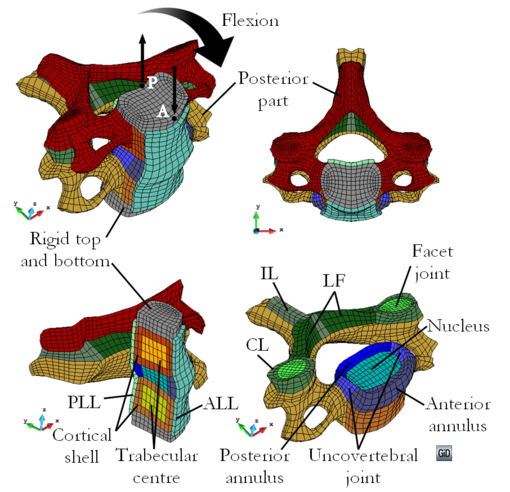
|
| Figure 60: – FSU meshed with Q1P0 elements. The components of the model and loading for flexion are detailed in the image. To impose extension loading, the flexion loading is reversed. |
A total of 9088 elements and 11389 nodes were required. The vertebrae were divided into the body and the posterior part, with the former composed of a nucleus of trabecular bone and a shell of cortical bone. The intervertebral disc was divided into the nucleus pulposus and the annulus fibrousus, with the latter further divided into anterior, lateral and posterior zones. The lateral parts of the annulus were treated as the uncovertebral joints. The anterior longitudinal ligament (ALL), the posterior longitudinal element (PLL), the ligamentum flavum (LF), the interspinous ligament (IL) and the capsular ligament (CL) were included in the model. The CL surrounds the facet joint. The top and bottom plates are rigid blocks on which to apply the loads to induce the rotations. All parts were modelled with the neo-Hookean hyperelastic constitutive model described in section 2.2.5, except the ligaments which were modelled with the Ogden hyperelastic constitutive model described in section 2.2.6. The neo-Hookean material parameter values were extracted from literature. Those reported as common to the cervical spine were considered [269,241,242,270] and are given in Table 14. To obtain the Ogden material parameters of the ligaments, analytic uniaxial tensile curves of the Ogden material (see section 2.2.4) were fitted to the stress-stretch curves available in Kallemeyn et al. [242] using the Matlab Curve Fitting Toolbox [108]. The fitted Ogden material parameters are given in Table 15 and the corresponding curves are plotted in Figure 61.
| Tissue | (MPa) | (MPa) |
| Cortical bone | 8330 | 1923 |
| Trabecular bone | 300 | 90 |
| Posterior bone | 2083 | 717 |
| Anterior annulus | 10 | 0.5 |
| Posterior annulus | 5 | 0.3 |
| Disc nucleus | 57 | 0.5 |
| Joints | 100 | 0.1 |
| Rigid plates |
| Ligament | (Pa) | (Pa) | (Pa) | |||
| ALL | 2.04 | 1.60 | 14.63 | 8.58 | 1.71 | 0.15 |
| PLL | 1.80 | 3.36 | 1.74 | 11.75 | 2.32 | 4.65 |
| IL | 2.90 | 8.52 | 1.16 | 15.20 | 0.51 | 2.22 |
| LF | 2.98 | 9.64 | 1.31 | 17.20 | 1.06 | 1.07 |
| CL | 5.73 | 9.50 | 3.59 | 20.00 | 4.90 | 0.10 |
![Cauchy stress vs. stretch of ligaments reported by Kallemeyn et al. [242] (lines) and fitted curves for the Ogden material model (crosses) to be used in the \mathrmC₄–\mathrmC₅ FSU model shown in Figure 60. The Ogden material parameters corresponding to the fitted curves are given in Table 15.](/wd/images/thumb/d/db/Draft_Samper_593843246-Ogden_Lig_Matlab.png/420px-Draft_Samper_593843246-Ogden_Lig_Matlab.png)
|
| Figure 61: Cauchy stress vs. stretch of ligaments reported by Kallemeyn et al. [242] (lines) and fitted curves for the Ogden material model (crosses) to be used in the – FSU model shown in Figure 60. The Ogden material parameters corresponding to the fitted curves are given in Table 15. |
A displacement-driven loading was applied in steps of 0.015mm on points A and P of the top rigid plate as indicated in Figure 60 to induce the flexion moment. A total of 100 steps were computed, which correspond to an approximate moment of 14Nm and about 13 of rotation. To induce the extension motion, the loading direction was reversed and 200 steps of 0.005mm were computed, which correspond to an approximate moment of -5Nm and about -9 of rotation.
The deformation and the strain distribution obtained in both cases (see Figure 62 and 64, respectively) show qualitatively correct results. The soft tissues (ligaments and intervertebral disc) absorb all the deformation while the hard tissues (bone) barely suffer deformation. However, to ensure the model is representative of a real FSU, its rotation vs. moment curve must fall within the experimental corridor published by Wheeldon et al. [235]. The displacements of the anterior point A and the posterior point P where the loads are applied (see Figure 60), and , respectively, are obtained in the output files for each load step. The reaction at these points is also given, and . The displacement-driven loading is vertical in all load steps, regardless of the inclination of the rigid top plate so the reaction vector for both points will only have vertical (axis) components. Hence, the moment can be computed as
|
|
(4.1) |
where is the distance between the two points, which is constant due to the rigid nature of the top plate. This distance should be, in fact, the projection of the distance between points A and P on the plane, which varies throughout the simulation. However, for simplicity, it has been assumed it is directly . This induces an error below 0.3% in both the flexion and extension cases for moment values below 2Nm, which is the maximum value given in the experimental corridors.
The rotation is computed knowing that the vertical displacement of the posterior and anterior points, and , respectively, are always in opposite directions, then
|
|
(4.2) |
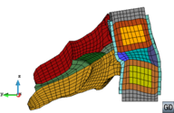
|
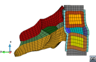
|
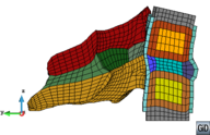
|
| Figure 62: Deformation of the – FSU subjected to flexo-extension loading. The parameters of the component materials are given in Tables 14 and 15. Half model is shown so that the internal deformation can be appreciated. The flexion results correspond to an approximate moment of 14Nm and about 13 of rotation. The extension results correspond to an approximate moment of -5Nm and about -9 of rotation. Extension (left), no deformation (centre) and flexion (right). Real deformation (1) is plotted. | ||
![Range of motion (or rotation) vs. applied flexo-extension moment results obtained for the \mathrmC₄–\mathrmC₅ FSU model shown in Figure 60. The parameters of the component materials are given in Tables 14 and 15. The mean experimental result and experimental corridors are taken from Wheeldon et al. [235].](/wd/images/thumb/3/35/Draft_Samper_593843246-Graph_FlexExt_init.png/420px-Draft_Samper_593843246-Graph_FlexExt_init.png)
|
| Figure 63: Range of motion (or rotation) vs. applied flexo-extension moment results obtained for the – FSU model shown in Figure 60. The parameters of the component materials are given in Tables 14 and 15. The mean experimental result and experimental corridors are taken from Wheeldon et al. [235]. |
The flexo-extension rotation vs. moment curves are plotted together with the experimental corridors in Figure 63. The nonlinearity of the response is captured but, even though the ligament curves obtained through the fitting are quite close to the ones available in literature, the flexion results from the FE model fall outside the experimental corridors. This can be explained by the fact that the curves used to reproduce the ligament behaviours were calibrated by Kallemeyn et al. [242] to fit their specific FE model. They model ligaments as nonlinear three-dimensional trusses with a certain cross-section. Scaling the material parameters according to the difference between the cross-section they considered and the approximate cross-section of the ligaments reproduced in our FE model improved the results. However, it became obvious that a more efficient way of computing adequate material parameters was required. The FSU model must be validated with the experimental curves and the material models used are phenomenological, so the main requirement is to identify the parameters that produce the desired result. This could be done by a manual trial-and-error procedure but, since, the whole process might have to be repeated anew when the FSU model of different vertebrae are developed or when a patient-specific geometry is required, it seems that automatizing the material identification process is a sensible choice.
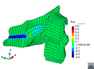
|
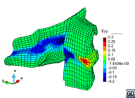
|
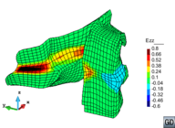
|
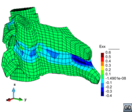
|
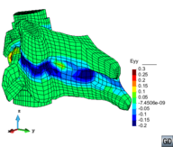
|
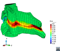
|
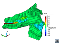
|
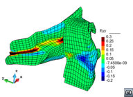
|
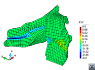
|
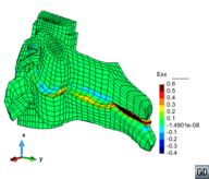
|
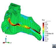
|
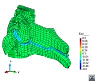
|
| Figure 64: Strain distributions of the – FSU subjected to flexo-extension loading. The parameters of the component materials are given in Tables 14 and 15. Half model is shown so that the internal distribution can be appreciated. The flexion results correspond to an approximate moment of 14Nm and about 13 of rotation. The extension results correspond to an approximate moment of -5Nm and about -9 of rotation. Real deformation (1) is plotted. | ||
(1) See section sec:SpineIntro of appendix ch:anatomy for a list and brief description of these ligaments.
4.3 Material parameter identification
To identify the material parameters of an FE model built to reproduce an experimental set-up, the numerical and experimental results are compared and, through a systematic adjustment of the parameters in the numerical model, the error between both results is minimized. Optimization techniques are used to aid in the adjustment of the parameters such that it is done in an optimal manner, reducing as much as possible the time required to reach the solution and the computational resources employed to that aim.
This procedure is essentially an inverse problem solved using computational techniques. Inverse problems consist in computing, from a set of results or observations, the causal factors or actions that produced them. Certain inverse problems can be solved analytically, however, for the present problem this is a complicated task of enormous mathematical complexity which is way beyond the objectives of this study. Therefore, and since we have numerous computational optimization tools at our disposal, the resolution of this problem is addressed from an optimization point of view.
First, an inverse method using a gradient-based optimization algorithm is developed to identify the material parameters of the FSU model described in the previous section that result in a rotation vs. moment response that falls inside the experimental corridors. Although developed independently, it is similar to the method proposed by Lei and Szeri [248]. The main algorithm is coded in Matlab [108] and coupled to the in-house FE code PLCd [1]. It uses a constrained nonlinear optimization algorithm available in the Matlab Optimization Toolbox. The details of this inverse method are described in section 4.3.1 and the method is used to identify the Ogden material parameters of the the FSU model.
Then, using the same basic concept, the method is restructured to be capable of identifying the material parameters of a damaged composite structure using an evolutionary algorithm. In this case, the main algorithm is written in Octave [271], which couples PLCd and the simple genetic algorithm Optimate [272], an in-house code developed at CIMAT (Center for Research in Mathematics in Guanajuato, Mexico). The details of this inverse method and its application to the identification of material parameters in composite materials is described in section 4.3.2.
4.3.1 Ogden material parameter identification using Matlab optimizer
The Matlab Optimization Toolbox [108] has been used to implement an optimizer which, linked to PLCd, calculates the value of the Ogden material parameters that result in a numerically obtained rotation vs. moment curve as close as possible to the mean experimental one from Wheeldon et al. [235]. Figure 65 presents the general scheme of the optimization method implemented in Matlab and its interaction with PLCd [1]. It is divided into three different blocks:
- The optimization function per se, implemented in Matlab (marked in blue in Figure 65).
- The FE calculations launched in PLCd for each iteration of the optimization function (marked in yellow in Figure 65).
- The experimental data used to calculate the optimizer's objective function (marked in green in Figure 65).
These three blocks can be viewed as independent units that interact with each other to form the proposed Ogden material parameter identification method.
![Scheme of the optimization method to obtain the Ogden parameters of the ligaments in the \mathrmC₄–\mathrmC₅ FSU. Algorithm implemented in Matlab [108] and that interacts with PLCd [1].](/wd/images/thumb/5/57/Draft_Samper_593843246-picture-6ac552.png/600px-Draft_Samper_593843246-picture-6ac552.png)
|
| Figure 65: Scheme of the optimization method to obtain the Ogden parameters of the ligaments in the – FSU. Algorithm implemented in Matlab [108] and that interacts with PLCd [1]. |
Optimizer module – Matlab The Matlab module is the method's core since it contains the optimization function that launches the FE calculations for each set of proposed parameters, adjusting their values according to the calculated objective function at the end, and launching a new set of parameters if the minimum has not been reached. In fact, the whole optimization process is initiated from Matlab.
The constrained nonlinear optimization algorithm fmincon available in the Matlab Optimization Toolbox has been used. The algorithm fmincon attempts to find a constrained minimum of a scalar function of several variables starting at an initial estimate, i.e., it finds the minimum of a problem specified by
|
|
(4.3) |
where is a nonlinear function that returns a scalar, namely, the objective function; is the vector of (normalized) material parameters to optimize; and and are the lower and upper band restrictions, respectively, of the optimization parameters . Detailed information on the options available for fmincon can be found in the on-line Matlab help website [108].
The sequential quadratic programming (sqp) algorithm has been chosen for the optimization and the step size factor has been set to . The objective function is defined as an norm such that the optimization algorithm will minimize the root mean squared error between the (mean) experimental curve – and numerical curve –. Hence, the objective function is
|
|
(4.4) |
where is the number of points available in the experimental data from Wheeldon et al. [235]. A small value is added to the denominator to avoid an indetermination for the initial point of the curve in which .
Prior to calculating this objective function, the following actions must be performed by the algorithm:
- Print the new material parameter values for this iteration in the adequate position of the FE input file.
- Launch the FE calculation.
- Read the displacement and reaction results obtained from the FE calculation and transform them into a curve using 4.1. At this point in the algorithm, the results are plotted and displayed on screen.
- Interpolate the vector at the values corresponding to .
This whole process is what fmincon considers as the objective function. Since the gradient of this function cannot be computed analytically, it is estimated using finite differences (FinDiffRelstep option). This implies that, for each iteration of the optimizer, PLCd will be launched at least once for each constraint considered plus an additional initial calculation. Therefore, it is of great importance that the number of optimization variables is reduced as much as possible.
In theory, there are at least thirty parameters to optimize (six Ogden material parameters for five different ligament materials). A sensitivity study performed on the parameters of each ligament revealed that there is one of the three pairs in each material that influences most the final shape of the corresponding Ogden curve. This is so because the Ogden material model computes the stress as the sum of three terms, each corresponding to a pair (see section 2.2.6). Then, plotting each of these terms separately for an uniaxial stress state showed that one of these three curves is much larger than the other two for all ligaments in the FSU model considered. It makes sense, thus, to ignore the less influential pairs in the optimization procedure since any changes they may suffer will have a minimal effect on the global response of the material behaviour.
Selecting only a pair of parameters to identify in each ligament, reduces to ten the number of optimization parameters to input in the fmincon algorithm. Then, the vector of (normalized) material parameters to optimize is
|
|
(4.5) |
where , being the value of the Ogden material parameter computed at each iteration of the optimizer and the initial value considered. The initial value of is equal to unity in all cases. The Ogden material parameters determined for the ligaments given in Table 15 were reported in the previous section such that the pair selected for optimization through the sensitivity study correspond to the first pair in all cases. Then, the value considered is the or value in Table 15 corresponding to each ligament.
No upper bound restriction is imposed for the optimization parameters and the lower bound restriction is defined as for all optimization parameters. This ensures that the Ogden material parameter being optimized does not change signs nor becomes zero. This restriction is more conservative than the original consistency condition 2.53 but easier to enforce in the optimization algorithm.
FE module – PLCd The FE code is not directly accessed by the user while the optimization process is working. However, previous to launching this process, the FE model must have been prepared to run in PLCd. This model corresponds to the – FSU unit described in section 4.2. The geometry, loads and boundary conditions are completely defined, as well as the desired output text files required to compute rotation vs. moment curves of the model. The constitutive model of each FSU component is fixed, with all material parameters defined except for the ones for which we seek the optimum value (described above). Then, Matlab accesses the PLCd input file to write the proposed parameter values and launch the FE calculation. Once the calculation is finished, Matlab accesses the output text files and post-processes the data to obtain the curves to be compared with the experimental mean curve.
The optimization problem described here was launched for the FSU model detailed in section 4.2. A total of 162 evaluations of the objective function were required, with each evaluation consuming approximately six minutes of computational time on an Intel(R) Core i7-2600 CPU @ 3.40GHz with 8GB of RAM. This results in approximately sixteen hours of calculation time for the optimizer to reach its goal. The value of the optimized material parameters is given in Table 16 and the flexo-extension rotation vs. moment curve obtained for these values is plotted, together with the initial curve, in Figure 66. The curve corresponding to the Ogden material parameters identified by the Matlab optimizer falls inside the experimental corridor, which was the objective of the optimization method proposed.
| Ligament | (Pa) | |
| ALL | 1.46 | 6.29 |
| PLL | 1.59 | 10.44 |
| IL | 2.38 | 4.04 |
| LF | 9.83 | 14.33 |
| CL | 4.85 | 25.06 |
![Range of motion vs. applied flexo-extension moment results obtained for the \mathrmC₄–\mathrmC₅ FSU model shown in Figure 60. The parameters of the component materials are given in Tables 14 and 15. The μ₁ and α₁ Ogen material parameters of the final curve correspond to those computed by the Matlab optimization algorithm described in Figure 65 and are given in Table 16. The mean experimental result and experimental corridors are taken from Wheeldon et al. [235].](/wd/images/thumb/a/a5/Draft_Samper_593843246-Graph_FlexExt_opt.png/420px-Draft_Samper_593843246-Graph_FlexExt_opt.png)
|
| Figure 66: Range of motion vs. applied flexo-extension moment results obtained for the – FSU model shown in Figure 60. The parameters of the component materials are given in Tables 14 and 15. The and Ogen material parameters of the final curve correspond to those computed by the Matlab optimization algorithm described in Figure 65 and are given in Table 16. The mean experimental result and experimental corridors are taken from Wheeldon et al. [235]. |
4.3.2 Composite material parameter identification using Optimate
The modular concept developed for the Ogden parameter identification using Matlab has been extended to a more general composite material parameter identification algorithm that uses an evolutionary optimization technique. The proposed optimization method for the determination of composite material parameters [273] is divided into three different blocks:
- The optimizer or optimization algorithm per se (marked in pink in Figure 67).
- The FEM calculations launched for each evaluation of the optimizer's objective function (marked in yellow in Figure 67).
- The experimental data used to calculate the optimizer's objective function (marked in green in Figure 67).
These three blocks can be understood as independent units which interact with each other to form the complete method, as schematized in Figure 67.
The optimizer used in block (1) is the in-house simple genetic algorithm Optimate [272]. It is coupled to an external objective function evaluator written in GNU Octave [271] (marked in orange in Figure 67). The external evaluator also acts as the interface with the in-house FE code PLCd [1] used in block (2). It launches the FEM calculation for each set of parameters proposed by Optimate and uses the results obtained to calculate the objective function which is fed back to Optimate. The calculation of the objective function requires the experimental data in block (3), which dictates the FE model to be used in block (2).
![Scheme of the proposed optimization method for the determination of damaged composite material parameters. Algorithm implemented in GNU Octave [271] that interacts with Optimate [272] and PLCd [1].](/wd/images/thumb/1/17/Draft_Samper_593843246-picture-584fcf.png/600px-Draft_Samper_593843246-picture-584fcf.png)
|
| Figure 67: Scheme of the proposed optimization method for the determination of damaged composite material parameters. Algorithm implemented in GNU Octave [271] that interacts with Optimate [272] and PLCd [1]. |
Experimental data The optimization method requires adequate experimental data with which to compare the numerical results in order to identify the correct material parameters. Since the experimental set-up must be reproduced in a FEA, it is essential that the geometrical details of the specimen used as well as the imposed boundary conditions are known. To calculate the objective function required by the optimizer, a simple load vs. displacement curve such as those obtained by standardized tensile tests suffices.
For the purpose of illustrating how the method works, an example is presented at the end of this section, based on the numerical data used by Car et al. [111]. In this way, the numerical result obtained can be validated. However, the methodology only requires the experimental data mentioned above to identify the material parameters of the FE model.
FE module – PLCd The FE code is not directly accessed by the user while the optimization process is working. However, previous to launching this process, the FE model must have been prepared to run in PLCd. This model must include a complete test specimen with the geometry, loads and boundary conditions completely defined, as well as the desired output results which will be used to calculate the FEM load vs. displacement curve.
The type of constitutive model to be used must be fixed for all materials, with all parameters defined except for the ones for which the optimum value is sought. That is, the type of constitutive models used to represent the behaviour of the component materials in the composite must be established a priori.
Optimizer module – Optimate The optimizer module includes the optimization program Optimate which seeks to minimize an objective function through evolutionary methods. This objective function is evaluated externally by the Optimate–PLCd interface written in GNU Octave.
This interface receives the optimization parameter values for the present evaluation of the objective function which correspond to the selected material parameters of the FE model. Then, the previously prepared PLCd input file is accessed, the new material values are written in the adequate positions of the file and the calculation is launched. Once the calculation is completed, GNU Octave accesses the output result file and post-processes the data to obtain the FEM curve, which is then compared to the experimental data. By means of an –norm estimation of the error between the two curves, the objective function is evaluated and the value obtained is fed back to Optimate.
The optimization algorithm developed in Optimate is a genetic algorithm with SBX [274] crossover, polynomial mutation, and binary tournament selection. These operators have been widely used in the well known NSGA-II [275] and omni-optimizer [276] algorithms for multi-objective optimization. The main algorithm is as follows:
- A random population is generated inside the search limits. The population size is denoted as .
- The objective function is evaluated for , obtaining the objective function vector .
- Using the binary tournament selection, a set of parents of size is selected as follows:
- Two individuals, and , are randomly chosen from and the objective function is evaluated for these individuals, and , respectively.
- If , then is selected for minimization; if , then is selected; otherwise, one of the two is selected randomly.
- The procedure is repeated until individuals have been selected.
- The selected individuals are denoted as .
- The crossover is applied. Using a Bernoulli experiment, the algorithm determines if the two parents are used for reproduction (with the crossover operator) or for cloning (a simple copy). If the parents are suitable for reproduction, another Bernoulli experiment is used per variable in order to decide if the operator is applied to it or not. Two consecutive parents in generate two children. This procedure is repeated until children are generated. The children population is denoted as . Two user-given parameters (probabilities) are required for this operation:
pcroind: probability of crossover for individuals.pcrovar: for two individuals selected for crossover, probability of applying the crossover operator to a variable of these individuals.
- The mutation is applied. The mutated population is denoted as as . Similar to the crossover, a Bernoulli experiment decides whether an individual is mutated or not, and another is used for each variable of an individual suited for mutation. Hence, two additional user-given parameters are required for this operation:
pcmutind: probability of mutation for individuals.pmutvar: for two individuals selected for mutation, probability of applying the mutation operator to a variable of these individuals.
- is evaluated and the new objective function values are denoted as .
- The old population is replaced with the best individuals obtained from the union of and .
- The procedure is repeated from step 3 until a stopping criterion is reached.
Three possible stopping criteria are defined for the algorithm. If one of these criteria is satisfied, the algorithm stops:
- A minimum objective function value to reach. If the best individual in the population has an objective function value less than a user-given value (
minObj), the algorithm stops.
- A minimum allowed variance of the objective function. The variance of the objective function is computed for each generation (iteration) and, for a given generation, if it is less than a user-given value (
maxVar), the algorithm stops.
- A number of iterations for which the minimum variance does not change. The minimum variance of the objective function values of the population from the beginning of the generations is computed and stored for each generation, if it does not change in a number of generations (user-given value,
minVarCount), the algorithm stops.
The –norm used to estimate the error between the experimental and FEM curves in order to obtain a value for the objective function is
|
|
(4.6) |
where represents the optimization parameters, are the displacement values of the curves, and and are the load values of the experimental and FEM curves for each , respectively. Since the displacement values at which the curves are compared must be the same, the experimental curve is linearly interpolated to the displacement values of the FEM curve. Obviously, the FEM calculation must be set up to obtain a certain number of displacement values such that the number of curve points used to determine the objective function is sufficient. Also, to avoid an indetermination for the first point of the curves, which is always zero, a very low value is added to the denominator.
Experimental data to validate the proposed optimization method has been taken from Car et al. [111]. The rectangular specimen with a double central notch is composed of carbon-epoxy T2300/914C with fibres oriented at with respect to the longitudinal axis of the sample. The problem is numerically reproduced using mixing theory in an infinitesimal strain framework. The material behaviour of the carbon fibres is modelled with an anisotropic elasto-plastic model while the material behaviour of the epoxy matrix is modelled with an isotropic explicit scalar damage model. For a detailed description of these constitutive models, see Comellas et al. [273].
The experimental set-up has been reproduced in FEA using standard 8-noded hexahedral solid elements. The model has been meshed with 897 elements and 1944 nodes, resulting in 5832 degrees of freedom and 7176 Gauss integration points. A displacement of 0.295mm has been imposed on the top nodes of the specimen in 25 equal increments, with the bottom nodes fully-fixed.
The material properties of both matrix and fibres are shown in Table 17, where TBD indicates the value of the properties which have been selected for the optimization method to determine. The Young's Modulus and Poisson coefficient indicated for the fibres correspond to the longitudinal direction of the fibres, in the transversal direction the values assigned are those of the epoxy matrix. The anisotropy stress transformation tensor is implemented in Voigt notation into the FE code and has been defined as a diagonal matrix with ones, except for , following the criterion used in the reference model [111].
| CARBON FIBRES | |
| Young's modulus, | TBD |
| Poisson coefficient, | |
| Yield stress, | TBD |
| Post yield behaviour law | Linear with hardening |
| Yield criterion | Von Mises |
| Hardening parameter, | TBD |
| Volumetric participation, |
| EPOXY MATRIX | |
| Young's modulus, | TBD |
| Poisson coefficient, | |
| Damage threshold stress, | TBD |
| Damage behaviour law | Exponential with softening |
| Damage (yield) criterion | Von Mises |
| Fracture energy, | TBD |
| Volumetric participation, |
The material parameters to be determined are normalized and introduced as optimization parameters of the optimizer. Since these parameters have a physical meaning, reasonable upper and lower limits have been imposed for each. This information is summarized in Table 18, together with the user-given parameters required by Optimate, already described in the previous pages.
| Material | Normalization | Lower | Upper |
| parameter | value | limit | limit |
| 1.0 | 5.0 | ||
| 1.0 | 30.0 | ||
| 1.0 | 10.0 | ||
| 1.0 | 5.0 | ||
| 0.2 | 0.6 | ||
| 0.1 | 1.0 |
| 100 | |
pcroind
|
0.9 |
pcrovar
|
0.85 |
pmutind
|
0.8 |
pmutvar
|
0.5 |
minObj
|
0.002 |
maxVar
|
|
minVarCount
|
20 |
The material parameters identified by the optimization method are reported in Table 19, which correspond to an objective function value of . The use of these parameters results in a load vs. displacement curve which matches the experimental one, as shown in Figure 68. The optimizer required 2860 evaluations of the objective function, with each evaluation requiring about half a minute of CPU time in a personal computer which uses an OpenSuse 12.3 operative system and is equipped with a 3.4GHz Intel(R) Core(TM) processor and 16GB RAM.
| Material | Normalized | Real |
| parameter | value | value |
| 3.982 | Pa | |
| 13.343 | Pa | |
| 9.428 | Pa | |
| 2.124 | Pa | |
| 0.374 | Pa | |
| 0.760 | N/m |
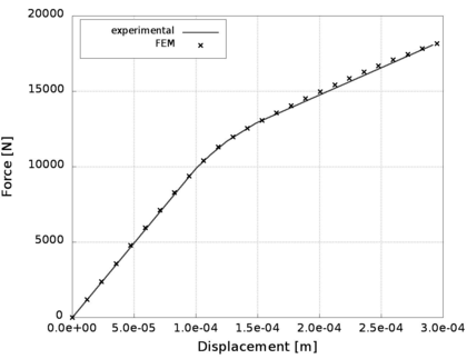
|
| Figure 68: Load vs. displacement curve for the FE model with the material parameters identified by the the proposed optimization method for the determination of composite material parameters. |
The material parameters identified using the proposed optimization method agree with the expected margin of values for these properties, as provided by manufacturers and seen in literature. Examination of the numerical result obtained also reveals expected behaviour of the specimen under loading, as shown in Figure 69. The displacement pattern obtained as well as the stress distributions closely match those of the reference model [111].
4.4 Discussion
The Ogden material parameter identification algorithm provides good results (see Figure 66), although there is room for improvement. The use of an norm means the objective function computed by the optimization algorithm is less restrictive than if an norm were considered. Unfortunately, for the case presented here, a change of norm would probably not produce a result closer to the mean experimental curve since it seems that a stiffer flexion curve (closer to the mean experimental one) would also produce a stiffer extension curve, which would probably then fall outside the experimental corridor.
This points to the need of revisiting the assumptions made to model the components of the FSU. In particular, the extension behaviour should be more pliable and the flexion one, stiffer. This could be achieved in several ways, although an in-depth study of the biomechanics of a FSU and the contribution of the different components to the overall flexo-extension behaviour is required in order to determine which is the best approach. A straightforward option is to consider altering the material parameter values of the anterior and posterior parts of the intervertebral disc's annulus. Another approach would be to introduce the composite modelling of the ligaments and intervertebral disc. If the fibres are accounted for through mixing theory, then anisotropy can be introduced into the model (see section 2.4.1) and, predictably, a differentiated response between flexion and extension could be achieved. These two options were tentatively tested and did not result in a significant improvement of the flexo-extension response. In addition, it seems that the uncovertebral and facet joints play a decisive important role in the motions of the FSU [277,278,279,280,281] and the present modelling of these joints is a crude representation of the complexity of a synovial joint. Hence, the ligament and disc improvement options were not fully pursued under the premise that a better modelling of the joints would probably result in more accurate FE results. This is further supported by the fact that the lateral flexion and axial rotation corridors, not considered in this study, are known to be coupled through the action of the facet joints. Then, if multi-objective optimization is to be used in the future in order to obtain material parameters that fit the corridors of the these three FSU motions, an improved FE model of the FSU is undoubtedly required.
Regarding the use of the gradient-based constrained nonlinear optimization algorithm available in the Matlab, it is reasonable to assume that the good results obtained are, in part, due to the good initial starting point. The initial value of the Ogden parameters to be optimized already produce a rotation vs. moment curve which falls inside the experimental corridor for extension and quite close to the corridor for flexion. It remains to be seen if the algorithm could reach a solution if the initial values produced a curve that fell far from the experimental corridor. Moreover, there is possibly not a unique solution to the optimization problem and the optimizer can easily fall in local minima of the objective function.
In view of this, and considering the known benefits of genetic algorithms over gradient-based ones (see section 4.1), the substitution of the Matlab algorithm for a genetic one such as Optimate seems like a sensible option. This approach has not been tested with the FSU problem, but the results obtained for the damaged composite specimen are promising. Of course, the damaged composite specimen is solved in an infinitesimal framework in PLCd [1] and, hence, the material constitutive models used do not exhibit the high nonlinearity of the hyperelastic formulations. Also, the requirement of limiting the possible values (the optimizer's search space) of the optimization parameters for material parameters that do not have a direct physical meaning such as the Ogden parameters might result in very large intervals of possible values, increasing considerably the computational cost.
In general, the bottleneck of the optimization method, especially if a genetic optimization algorithm is employed, is the computational cost of each FE computation, which hinders the computational cost of the overall procedure. In the genetic optimization method, a complete FE computation is required for each evaluation of the objective function, and the optimization method requires a significant number of evaluations. In the case of the gradient-based method, a smaller amount of evaluations of the objective function may be needed to reach a solution, but each evaluation requires at least as many evaluations as optimization parameters considered. Consequently, certain FE models might result prohibitive to work with. In the particular cases exposed in this chapter, the reduction of the computation time of each FEM calculation was already tackled through the parallelization of the PLCd code using OpenMP. In some cases, the symmetry of the model and its loading conditions may be exploited to reduce the size of the computational problem. In any case, a compromise must be reached between accuracy and computational efficiency when it comes to numerically reproducing the experimental set-up.
4.5 Conclusions
An inverse method that provides a way of identifying the material properties of FE phenomenological constitutive models such that they fit known experimental data is proposed. This method is developed, first, for the identification of the Ogden material parameters in ligaments of a – FSU using a gradient-based optimization algorithm available in the Matlab Optimization Toolbox, and, then, for the identification of the material parameters in damaged composite structures using the genetic optimization algorithm Optimate.
The methodology proposed is highly flexible due to its modular structure. The codes both for the FEM calculation and optimization algorithm can be easily replaced by other in-house or commercial equivalent softwares. I addition, the experimental data and equivalent numerical model may also be changed, requiring only minor modifications in the interface code. This, in fact, has been exemplified by using the same basic structure to develop, on the one hand, a gradient-based optimization method to identify the Ogden material parameters in the FSU and, on the other, a genetic optimization method to identify the material parameters of a damaged composite structure.
The examples presented in this chapter evidence the applicability of optimization techniques in the determination of adequate material parameters to represent known experimental set-ups. However, developing a robust, efficient and fast method for this purpose is not a trivial endeavour. The type of optimization algorithm, the selection of the material parameters to optimize, the definition of a suitable objective function and the modelling assumptions used in the FE reproduction of the experimental set-up must be tailored to each particular application in order to exploit the full potentiality of this type of approach.
5 Conclusions
5.1 Achievements
The aim of this study was to set the bases for a general constitutive formulation capable of representing the behaviour of soft biological tissue through numerical simulation using the in-house FE code PLCd [1]. This has been achieved by means of the generalized mixing theory in conjunction with phenomenological models to represent both the passive and active behaviours of tissues. Thus, soft biological tissue has been treated as a composite material formed by collagen fibres embedded in an extracellular matrix. The behaviour of each individual component is reproduced using a phenomenological constitutive model and, then, the generalized mixing theory produces the global tissue behaviour.
The constitutive modelling of passive properties has been addressed in Chapter 2. Neo-hookean and Ogden hyperelasticity formulations have been implemented in PLCd, which have served as basis for the rest of constitutive models developed in this study. To complete the characterization of passive behaviour in soft tissues, a generalized finite-strain damage model [106] has been developed. It has been particularized for neo-Hookean and Ogden hyperelasticity, implemented in PLCd and validated through numerical examples. Finally, the use of generalized mixing theory to represent soft tissue behaviour has been described and the use of a tensile/compressive switch and space mapping to account for anisotropic behaviour has been proposed.
The constitutive modelling of the active properties has been addressed in Chapter 3. The basic active properties of growth and remodelling have been reproduced by means of two different constitutive models which can be viewed as an extension of the passive models described in the previous chapter. An existing volumetric growth model considering biological availability has been particularized for Ogden hyperelasticity and implemented in PLCd. Then, it has been extended to include anisotropy in the direction of growth [196]. Regarding the remodelling phenomena, a novel constitutive model for homeostatic-driven turnover remodelling in soft tissues [282] has been presented and discussed. The formulation has been particularized for Ogden hyperelasticity, implemented in PLCd and validated through numerical examples. Finally, the integration of these two new models to obtain a more general constitutive formulation to represent active behaviour in soft biological tissue has been discussed.
The identification of the material parameters in phenomenological constitutive models has been addressed in Chapter 4. The difficulties encountered in the FE modelling of a cervical spine are presented [234], namely, the need to correctly identify the material parameters in the constitutive models used. For this purpose, an inverse method using optimization techniques has been developed and discussed. The method has been coupled to a gradient-based optimization algorithm available in Matlab and to the population-based evolutionary algorithm Optimate [273], and the strengths and weaknesses of each have been identified.
5.2 Concluding remarks
The generalized mixing theory evaluates the interaction of the different material components at stress level. It works, thus, as a “constitutive model manager” that allows evaluating the interaction of the different constitutive models that represent each component's behaviour (matrix and fibres) to obtain the overall composite behaviour (biological tissue). Used in conjunction with a series of phenomenological models capable of spanning a large scope of material behaviours, it is a powerful tool in achieving a general multi-purpose constitutive formulation for representing soft tissue behaviour.
We believe the generalized approach allows for more flexibility in composing the overall behaviour of the tissue since new constitutive models to represent fibre or matrix behaviour can be easily introduced if required. In this sense, an initial library of constitutive equations to represent the basic characteristics of soft biological tissues has been introduced in PLCd [1]. This library includes phenomenological models developed in a finite strain framework that account for the non-linear, damage, growth and remodelling behaviours. These were selected for the initial library because they were regarded as the “essential” mechanobiological characteristics observed in living tissues.
Given the limited availability of experimental mechanical information and the difficulties associated with the estimation of parameters, we sought a general overall formulation built upon relatively simple constitutive models but capable of reproducing a wide range of soft tissue behaviour. In addition to their straightforward formulation, the phenomenological models introduced have the advantage of being built on a solid and established thermodynamic basis, which allows for better tracing of the individual component's thermomechanical behaviour.
Nonetheless, the models implemented throughout this study merely constitute the seedbed of the general constitutive framework described in this study. The library of constitutive equations can and should be extended to include more models in order to widen the scope of representation of the formulation. Conversely, models can also be added to particularize the formulation for specific applications, if required. It is an ambitious goal, but we believe the foundations established in this study are solid enough to sustain such enterprise.
Biological tissues are complex hierarchical structures that have the capacity of evolving in response to external loads and environmental stimuli. The inter-relations between the mechanical and biological processes that take place in tissues is not fully understood yet and is an active multi-disciplinary area of research. As a deeper understanding of the processes occurring at molecular and cellular level is attained, the use of phenomenological models might have to be set aside in favour of multi-scale homogenization and/or mechanistic models for the simple constituent materials.
At present, though, and in view of the aims set for this study, the constitutive models proposed, phenomenological in nature, seem like the best choice because they manage to produce a general constitutive formulation for biological tissues. This formulation spans a large scope of tissue behaviour and solely requires the identification of a series of parameters whose identification, given adequate experimental data, can be automatized by means of inverse methods that use optimization techniques.
In conclusion, the bases for a general constitutive formulation capable of representing soft biological tissue behaviour have been set successfully. The most notable contribution is probably the coupling of the mechanical and metabolic fields in the models developed to account for the active behaviour of tissues. The numerical examples presented validate the formulations developed and demonstrate their applicability in biomechanical studies.
5.3 Future work
The framework built for the general constitutive formulation is an excellent basis for future developments. Some of these have already been pointed out and discussed throughout the monography.
In the first place, there is always room for improvement in an in-house code such as PLCd [1] from a numerical perspective. Any modification that can improve the robustness and accuracy of the calculations, such as an upgrading of the mixed u/p elements used, is welcome. The automatization of the particularization of the damage, growth and healing models to any desired hyperelastic formulation implemented in the code would also be a useful feature, generalizing even more the framework developed.
Regarding the passive behaviour of soft tissues, the hyperelastic and finite-strain damage formulations implemented could be extended to include other alternatives which might result useful in future applications. In particular, viscoelasticity could be introduced in the hyperelastic formulation and a continuous damage variable could be added into the damage formulation to account for the Mullins effect. Needless to say that additional damage evolution laws could also be included in the damage model to particularize the formulation to represent specific tissue behaviour.
As to the active behaviour of tissues, if experimental data becomes available, both growth and healing models could be expanded with new expressions of the growth stretch evolution and healing rate, respectively, tailored to these particular applications. Also, a constitutive model that accounts for the fibre-reorientation observed in most remodelling processes could be introduced to complete the representation of active properties in tissues. In addition, the modelling of biological availability in these models could be refined, based on mechanobiological observations, to better represent the metabolism of living tissues.
Finally, the inverse method using optimization techniques developed could be extended to include multi-objective optimization in order to improve the parameter identification results. In addition, it would be interesting to conduct a thorough study of the sensitivity and uniqueness of the solution obtained and how the objective function selected for the optimization method affects the results. This is especially important in the case of non-linear material models such as the ones considered in this study since they are known to have more than one optimal set of parameters in many applications.
References
[1] PLCd research group "PLCd: Non-linear thermo-mechanic finite element code for research-oriented applications". Free access code developed at CIMNE. Available at: http://www.cimne.com/PLCd. 1991 to present.
[2] Bathe, Klaus-Jürgen and Ramm, Ekkehard and Wilson, Edward L. (1975) "Finite element formulations for large deformation dynamic analysis", Volume 9. International Journal for Numerical Methods in Engineering 2 353–386
[3] Fung, Y C. (1993) "Biomechanics: mechanical properties of living tissues". Springer-Verlag, 2 Edition
[4] Viceconti, Marco. (2015) "Biomechanics-based in silico medicine: the manifesto of a new science.", Volume 48. Journal of Biomechanics 2 193–194
[5] Zienkiewicz, Olgierd Cecil and Taylor, Robert L. (1989) "The Finite Element Method. Vol I and II.". McGraw-Hall
[6] Malvern, Lawrence E. (1969) "Introduction to the mechanics of a continuous medium". Prentice-Hall
[7] Doblaré, Manuel and García-Aznar, José Manuel. (2010) "Modelling Living Tissues: Mechanical and Mechanobiological Aspects", Volume 15. Progress in Industrial Mathematics at ECMI 2008. Springer Berlin Heidelberg 3–8
[8] Humphrey, J D and Yin, F C P. (1987) "A new constitutive formulation for characterizing the mechanical behavior of soft tissues", Volume 52. Biophysical Journal 4 563–570
[9] Oller, Sergio. (2014) "Numerical Simulation of Mechanical Behavior of Composite Materials". Springer-CIMNE 240
[10] Schenk, Olaf and Gärtner, Klaus. (2004) "Solving unsymmetric sparse systems of linear equations with PARDISO", Volume 20. Future Generation Computer Systems 3 475–487
[11] Humphrey, J. D. (2003) "Review Paper: Continuum biomechanics of soft biological tissues", Volume 459. Proceedings of the Royal Society A: Mathematical, Physical and Engineering Sciences 2029 3–46
[12] Fung, Y C. (1967) "Elasticity of soft tissues in simple elongation.", Volume 213. The American Journal of Physiology 6 1532–1544
[13] Steinmann, P and Hossain, M and Possart, G. (2012) "Hyperelastic models for rubber-like materials: Consistent tangent operators and suitability for Treloar's data", Volume 82. Archive of Applied Mechanics 9 1183–1217
[14] Chagnon, G. and Rebouah, M. and Favier, D. (2014) "Hyperelastic Energy Densities for Soft Biological Tissues: A Review", Volume 120. Journal of Elasticity 2 129–160
[15] Auricchio, F. and Ferrara, A. and Morganti, S. (2012) "Comparison and critical analysis of invariant-based models with respect to their ability in fitting human aortic valve data", Volume 4. Annals of Solid and Structural Mechanics 1-2 1–14
[16] Vaishnav, R N and Young, J T and Patel, D J. (1973) "Distribution of stresses and of strain-energy density through the wall thickness in a canine aortic segment.", Volume 32. Circulation Research 1 577–583
[17] Fung, Y. C. and Fronek, K. and Patitucci, P. (1979) "Pseudoelasticity of arteries and the choice of its mathematical expression.", Volume 237. The American Journal of Physiology 5 H620–H631
[18] Takamizawa, Keiichi and Hayashi, Kozaburo. (1987) "Strain energy density function and uniform strain hypothesis for arterial mechanics", Volume 20. Journal of Biomechanics 1 7–17
[19] Holzapfel, Gerhard A. (2000) "Nonlinear solid mechanics: a continuum approach for engineering". John Wiley & Sons
[20] Spencer, A.J.M. (1984) "Constitutive theory for strongly anisotropic solids". Continuum Theory of the Mechanics of Fibre-Reinforced Composites. Springer Vienna 1–32
[21] Holzapfel, G. a. and Gasser, T. C. and Stadler, M. (2002) "A structural model for the viscoelastic behavior of arterial walls: Continuum formulation and finite element analysis", Volume 21. European Journal of Mechanics - A/Solids 3 441–463
[22] Limbert, Georges and Middleton, John. (2004) "A transversely isotropic viscohyperelastic material: Application to the modeling of biological soft connective tissues", Volume 41. International Journal of Solids and Structures 15 4237–4260
[23] Peña, E. and Calvo, B. and Martínez, M.A. and Doblaré, M. (2007) "An anisotropic visco-hyperelastic model for ligaments at finite strains. Formulation and computational aspects", Volume 44. International Journal of Solids and Structures 3-4 760–778
[24] Gasser, T. Christian and Forsell, Caroline. (2011) "The numerical implementation of invariant-based viscoelastic formulations at finite strains. An anisotropic model for the passive myocardium", Volume 200. Computer Methods in Applied Mechanics and Engineering 49-52 3637–3645
[25] Ahsanizadeh, Sahand and Li, LePing. (2015) "Visco-hyperelastic constitutive modeling of soft tissues based on short and long-term internal variables", Volume 14. BioMedical Engineering OnLine 1 29
[26] Limbert, Georges and Taylor, Mark. (2002) "On the constitutive modeling of biological soft connective tissues: A general theoretical framework and explicit forms of the tensors of elasticity for strongly anisotropic continuum fiber-reinforced composites at finite strain", Volume 39. International Journal of Solids and Structures 8 2343–2358
[27] Natali, A N and Pavan, P G and Carniel, E L and Lucisano, M E and Taglialavoro, G. (2005) "Anisotropic elasto-damage constitutive model for the biomechanical analysis of tendons", Volume 27. Medical Engineering & Physics 3 209–214
[28] Calvo, B and Peña, Estefanía and Martínez, M A and Doblaré, Manuel. (2007) "An uncoupled directional damage model for fibred biological soft tissues. Formulation and computational aspects", Volume 69. International Journal for Numerical Methods in Engineering 10 2036–2057
[29] Peña, Estefanía and Peña, Juan A and Doblaré, Manuel. (2009) "On the Mullins effect and hysteresis of fibered biological materials: A comparison between continuous and discontinuous damage models", Volume 46. International Journal of Solids and Structures 7-8 1727–1735
[30] Balzani, Daniel and Brinkhues, Sarah and Holzapfel, Gerhard A. (2012) "Constitutive framework for the modeling of damage in collagenous soft tissues with application to arterial walls", Volume 213-216. Computer Methods in Applied Mechanics and Engineering 0 139–151
[31] Gasser, T. Christian. (2011) "An irreversible constitutive model for fibrous soft biological tissue: A 3-D microfiber approach with demonstrative application to abdominal aortic aneurysms", Volume 7. Acta Materialia Inc. Acta Biomaterialia 6 2457–2466
[32] Peña, Estefanía. (2011) "A rate dependent directional damage model for fibred materials: application to soft biological tissues", Volume 48. Computational Mechanics 4 407–420
[33] Mullins, L. (1948) "Effect of Stretching on the Properties of Rubber", Volume 21. Rubber Chemistry and Technology 2 281–300
[34] Diani, Julie and Fayolle, Bruno and Gilormini, Pierre. (2009) "A review on the Mullins effect", Volume 45. European Polymer Journal 3 601–612
[35] Peña, Estefanía. (2011) "Prediction of the softening and damage effects with permanent set in fibrous biological materials", Volume 59. Journal of the Mechanics and Physics of Solids 9 1808–1822
[36] Ogden, R W. (1997) "Non-linear elastic deformations". Dover Publications
[37] Crisfield, M A. (1991) "Non-linear finite element analysis of solids and structures". John Wiley & Sons
[38] Bower, Allan F. (2010) "Applied mechanics of solids". CRC Press
[39] Bathe, Klaus-Jürgen. (1982) "Finite element procedures in engineering analysis". Prentice-Hall 735
[40] Belytschko, Ted and Liu, W K and Moran, Brian. (2000) "Nonlinear finite elements for continua and structures". John Wiley & Sons 650
[41] Ní Annaidh, A and Destrade, M and Gilchrist, M D and Murphy, J G. (2013) "Deficiencies in numerical models of anisotropic nonlinearly elastic materials.", Volume 12. Biomechanics and Modeling in Mechanobiology 4 781–791
[42] Pierrat, B. and Murphy, J.G. and MacManus, D.B. and Gilchrist, M.D. (2015) "Finite element implementation of a new model of slight compressibility for transversely isotropic materials". Taylor & Francis. Computer Methods in Biomechanics and Biomedical Engineering
[43] Simo, Juan C and Taylor, Robert L. (1991) "Quasi-incompressible finite elasticity in principal stretches. Continuum basis and numerical algorithms", Volume 85. Computer Methods in Applied Mechanics and Engineering 3 273–310
[44] Gadala, M S. (1992) "Alternative methods for the solution of hyperelastic problems with incompressibility", Volume 42. Computers & Structures 1 1–10
[45] Miehe, C. (1994) "Aspects of the formulation and finite element implementation of large strain isotropic elasticity", Volume 37. International Journal for Numerical Methods in Engineering 12 1981–2004
[46] Sussman, Theodore and Bathe, Klaus-Jürgen. (1987) "A finite element formulation for nonlinear incompressible elastic and inelastic analysis", Volume 26. Computers & Structures 1/2 357–409
[47] Bonet, Javier and Wood, Richard D. (2008) "Nonlinear Continuum Mechanics for Finite Element Analysis". Cambridge University Press 318, 2 Edition
[48] Auricchio, Ferdinando and Da Veiga, Lourenco Beirao and Lovadina, Carlo and Reali, Alessandro and Taylor, Robert L. and Wriggers, Peter. (2013) "Approximation of incompressible large deformation elastic problems: some unresolved issues", Volume 52. Computational Mechanics 5 1153–1167
[49] Oñate, Eugenio. (1995) "Cálculo de estructuras por el método de los elementos finitos: análisis estático lineal". Ed. CIMNE 838, 2 Edition
[50] Bonet, Javier. (1998) "A simple average nodal pressure tetrahedral element for incompressible and nearly incompressible dynamic explicit applications", Volume 14. Communications in Numerical Methods in Engineering 5 437–449
[51] Bonet, Javier. (2001) "An averaged nodal deformation gradient linear tetrahedral element for large strain explicit dynamic applications", Volume 17. Communications in Numerical Methods in Engineering 8 551–561
[52] Joldes, Grand Roman and Wittek, Adam and Miller, Karol. (2009) "Non-locking tetrahedral finite element for surgical simulation", Volume 25. Communications in Numerical Methods in Engineering 7 827–836
[53] Frémond, Michel. (2006) "The Clausius-Duhem Inequality, an Interesting and Productive Inequality", Volume 12. Nonsmooth Mechanics and Analysis. Springer US 107–118
[54] Coleman, Bernard D. and Gurtin, Morton E. (1967) "Thermodynamics with Internal State Variables", Volume 47. AIP Publishing. The Journal of Chemical Physics 2 597–613
[55] Miehe, Christian. (1996) "Numerical computation of algorithmic (consistent) tangent moduli in large-strain computational inelasticity", Volume 134. Computer Methods in Applied Mechanics and Engineering 3-4 223–240
[56] Treloar, L. R. G. (1944) "Stress-strain data for vulcanised rubber under various types of deformation", Volume 40. The Royal Society of Chemistry. Transactions of the Faraday Society 59
[57] Mooney, M. (1940) "A Theory of Large Elastic Deformation", Volume 11. AIP Publishing. Journal of Applied Physics 9 582–592
[58] Rivlin, R. S. (1948) "Large Elastic Deformations of Isotropic Materials. IV. Further Developments of the General Theory", Volume 241. Philosophical Transactions of the Royal Society A: Mathematical, Physical and Engineering Sciences 835 379–397
[59] Liu, I-Shih. (2011) "A note on the Mooney-Rivlin material model", Volume 24. Continuum Mechanics and Thermodynamics 4-6 583–590
[60] Yeoh, O. H. (1993) "Some Forms of the Strain Energy Function for Rubber", Volume 66. Rubber Chemistry and Technology 5 754–771
[61] Veronda, D.R. and Westmann, R.A. (1970) "Mechanical characterization of skin - Finite deformations", Volume 3. Elsevier. Journal of Biomechanics 1 111–124
[62] Ogden, R. W. (1972) "Large Deformation Isotropic Elasticity - On the Correlation of Theory and Experiment for Incompressible Rubberlike Solids", Volume 326. Proceedings of the Royal Society A: Mathematical, Physical and Engineering Sciences 1567 565–584
[63] Chui, C. and Kobayashi, E. and Chen, X. and Hisada, T. and Sakuma, I. (2004) "Combined compression and elongation experiments and non-linear modelling of liver tissue for surgical simulation", Volume 42. Medical & Biological Engineering & Computing 6 787–798
[64] Martins, P A L S and Jorge, R M N and Ferreira, A J M. (2006) "A comparative study of several material models for prediction of hyperelastic properties: Application to silicone-rubber and soft tissues", Volume 42. Strain 3 135–147
[65] Wex, Cora and Arndt, Susann and Stoll, Anke and Bruns, Christiane and Kupriyanova, Yuliya. (2015) "Isotropic incompressible hyperelastic models for modelling the mechanical behaviour of biological tissues: a review.". Biomedizinische Technik. Biomedical engineering
[66] Ogden, R. W. and Saccomandi, G. and Sgura, I. (2004) "Fitting hyperelastic models to experimental data", Volume 34. Computational Mechanics 6 484–502
[67] Coll, A. and Ribó, R. and Pasenau, M. and Escolano, E. and Perez, J.Suit. and Melendo, A. and Monros, A. (2014) "GiD v.12 Reference Manual". CIMNE
[68] Chaboche, J L. (1988) "Continuum Damage Mechanics: Part I–General Concepts", Volume 55. Journal of Applied Mechanics 1 59–64
[69] Simo, Juan C and Ju, J W. (1987) "Strain- and stress-based continuum damage models–I. Formulation", Volume 23. International Journal of Solids and Structures 7 821–840
[70] Kachanov, L M. (1999) "Rupture Time Under Creep Conditions", Volume 97. International Journal of Fracture 1 11–18
[71] Kachanov, L. M. (1986) "Introduction to continuum damage mechanics", Volume 10. Springer Netherlands
[72] Lemaitre, Jean. (1996) "A Course on Damage Mechanics". Springer Berlin Heidelberg
[73] Murakami, S. (1983) "Notion of Continuum Damage Mechanics and its Application to Anisotropic Creep Damage Theory", Volume 105. American Society of Mechanical Engineers. Journal of Engineering Materials and Technology 2 99
[74] Ju, J. W. (1990) "Isotropic and Anisotropic Damage Variables in Continuum Damage Mechanics", Volume 116. American Society of Civil Engineers. Journal of Engineering Mechanics 12 2764–2770
[75] Lemaitre, Jean. (1985) "Coupled elasto-plasticity and damage constitutive equations", Volume 51. Computer Methods in Applied Mechanics and Engineering 1-3 31–49
[76] Ju, J.W. (1989) "On energy-based coupled elastoplastic damage theories: Constitutive modeling and computational aspects", Volume 25. International Journal of Solids and Structures 7 803–833
[77] Oller, Sergio and Oliver, Javier and Lubliner, J and Oñate, Eugenio. (1988) "Un modelo constitutivo de daño plástico para materiales friccionales. Parte - I: Variables fundamentales, funciones de fluencia y potencial", Volume 4. Revista Internacional de Métodos Numéricos para Cálculo y Diseño en Ingeniería 4 397–431
[78] Faria, R. and Oliver, J. and Cervera, M. (1998) "A strain-based plastic viscous-damage model for massive concrete structures", Volume 35. International Journal of Solids and Structures 14 1533–1558
[79] Lubliner, J. and Oliver, J. and Oller, S. and Oñate, E. (1989) "A plastic-damage model for concrete", Volume 25. International Journal of Solids and Structures 3 299–326
[80] Ortiz, Michael. (1985) "A constitutive theory for the inelastic behavior of concrete", Volume 4. Mechanics of Materials 1 67–93
[81] Oller, Sergio and Oñate, E. and Miquel, J. and Botello, S. (1996) "A plastic damage constitutive model for composite materials", Volume 33. International Journal of Solids and Structures 17 2501–2518
[82] Hokanson, J and Yazdani, S. (1997) "A constitutive model of the artery with damage", Volume 24. Mechanics Research Communications 2 151–159
[83] Miehe, C. (1995) "Discontinuous and continuous damage evolution in Ogden-type large-strain elastic materials", Volume 14. European Journal of Mechanics - A/Solids 5 697–720
[84] Souza Neto, E A and Peri, D and Owen, D R J. (1998) "Continuum modelling and numerical simulation of material damage at finite strains", Volume 5. Archives of Computational Methods in Engineering 4 311–384
[85] Peña, Estefanía. (2011) "Damage functions of the internal variables for soft biological fibred tissues", Volume 38. Mechanics Research Communications 8 610–615
[86] Martins, P and Peña, E and Jorge, R M Natal and Santos, A and Santos, L and Mascarenhas, T and Calvo, B. (2012) "Mechanical characterization and constitutive modelling of the damage process in rectus sheath.", Volume 8. Journal of the Mechanical Behavior of Biomedical Materials 111–122
[87] Blanco, Sergio and Polindara, César Andrés and Goicolea, Jose María. (2015) "A regularised continuum damage model based on the mesoscopic scale for soft tissue", Volume 58. International Journal of Solids and Structures 20–33
[88] Simo, Juan C. (1987) "On a fully three-dimensional finite-strain viscoelastic damage model: Formulation and computational aspects", Volume 60. Computer Methods in Applied Mechanics and Engineering 2 153–173
[89] El Sayed, Tamer and Mota, Alejandro and Fraternali, Fernando and Ortiz, Michael. (2008) "A variational constitutive model for soft biological tissues", Volume 41. Journal of Biomechanics 7 1458–1466
[90] El Sayed, Tamer and Mota, Alejandro and Fraternali, Fernando and Ortiz, Michael. (2008) "Biomechanics of traumatic brain injury", Volume 197. Computer Methods in Applied Mechanics and Engineering 51-52 4692–4701
[91] Horgan, C. O. and Murphy, J. G. (2011) "Simple shearing of soft biological tissues", Volume 467. Proceedings of the Royal Society A: Mathematical, Physical and Engineering Sciences 2127 760–777
[92] Peña, Estefanía and Doblaré, Manuel. (2009) "An anisotropic pseudo-elastic approach for modelling Mullins effect in fibrous biological materials", Volume 36. Mechanics Research Communications 7 784–790
[93] Ehret, Alexander E. and Itskov, Mikhail. (2009) "Modeling of anisotropic softening phenomena: Application to soft biological tissues", Volume 25. International Journal of Plasticity 5 901–919
[94] Peña, Estefanía. (2014) "Computational aspects of the numerical modelling of softening, damage and permanent set in soft biological tissues", Volume 130. Computers & Structures 57–72
[95] Aubard, X. and Boucard, P.-A. -A and Ladeveze, P. and Michel, S. (2002) "Modeling and simulation of damage in elastomer structures at high strains", Volume 80. Computers & Structures 27-30 2289–2298
[96] Alastrué, V. and Rodríguez, J.F. and Calvo, B. and Doblaré, M. (2007) "Structural damage models for fibrous biological soft tissues", Volume 44. International Journal of Solids and Structures 18-19 5894–5911
[97] Natali, A.N. and Pavan, P.G. and Carniel, E.L. and Dorow, C. (2003) "A Transversally Isotropic Elasto-damage Constitutive Model for the Periodontal Ligament", Volume 6. Computer Methods in Biomechanics and Biomedical Engineering 5-6 329–336
[98] Balzani, Daniel and Schröder, J and Gross, D. (2006) "Simulation of discontinuous damage incorporating residual stresses in circumferentially overstretched atherosclerotic arteries", Volume 2. Acta Biomaterialia 6 609–618
[99] Famaey, N and Sloten, J Vander and Kuhl, Ellen. (2013) "A three-constituent damage model for arterial clamping in computer-assisted surgery", Volume 12. Biomechanics and Modeling in Mechanobiology 1 123–136
[100] Peña, E and Calvo, B and Martínez, M A and Doblaré, M. (2008) "On finite-strain damage of viscoelastic-fibred materials. Application to soft biological tissues", Volume 74. International Journal for Numerical Methods in Engineering 7 1198–1218
[101] Rodríguez, José F and Cacho, Fernando and Bea, José A and Doblaré, Manuel. (2006) "A stochastic-structurally based three dimensional finite-strain damage model for fibrous soft tissue", Volume 54. Journal of the Mechanics and Physics of Solids 4 864–886
[102] Balzani, D. and Schmidt, T. (2013) "Comparative analysis of damage functions for soft tissues: Properties at damage initialization", Volume 20. Mathematics and Mechanics of Solids 4 480–492
[103] Oliver, Javier and Cervera, Miguel and Oller, Sergio and Lubliner, J. (1990) "Isotropic damage models and smeared crack analysis of concrete". Proc. SCI-C Computer Aided Analysis and Design of Concrete Structures 945–957
[104] Oller, Sergio. (2014) "Nonlinear Dynamics of Structures". Springer-CIMNE 197–203
[105] Oller, Sergio. (2001) "Fractura mecánica: un enfoque global". Centre Internacional de Metodes Numerics en l'Enginyeria (CIMNE) and Universitat Politecnica de Catalunya
[106] Comellas, Ester and Bellomo, Facundo and Oller, Sergio. (2015) "A generalized finite-strain damage model for quasi-incompressible hyperelasticity using hybrid formulation". International Journal for Numerical Methods in Engineering
[107] Truesdell, C. and Toupin, R. (1960) "The Classical Field Theories". Principles of Classical Mechanics and Field Theory / Prinzipien der Klassischen Mechanik und Feldtheorie. Springer Berlin Heidelberg 226–858
[108] MathWorks "MATLAB, Optimization Toolbox and Curve Fitting Toolbox for technical computing". The MathWorks Inc.
[109] Holzapfel, Gerhard A. and Ogden, Ray W. (2015) "On the tension-compression switch in soft fibrous solids", Volume 49. European Journal of Mechanics - A/Solids 561–569
[110] Oller, Sergio and Botello, S. and Miquel, J. and Oñate, E. (1995) "An anisotropic elastoplastic model based on an isotropic formulation", Volume 12. MCB UP Ltd. Engineering Computations 3 245–262
[111] Car, E. and Oller, Sergio and Oñate, E. (2000) "An anisotropic elastoplastic constitutive model for large strain analysis of fiber reinforced composite materials", Volume 185. Computer Methods in Applied Mechanics and Engineering 2-4 245–277
[112] Car, E. and Oller, S. and Oñate, E. (2001) "A large strain plasticity model for anisotropic materials - A composite material application", Volume 17. International Journal of Plasticity 11 1437–1463
[113] Betten, Josef. (1981) "Creep Theory of Anisotropic Solids", Volume 25. The Society of Rheology. Journal of Rheology 6 565
[114] Humphrey, J D and Rajagopal, K R. (2002) "A constrained mixture model for growth and remodelling of soft tissues", Volume 12. Mathematical Models and Methods in Applied Sciences 03 407–430
[115] Thompson, D. W. (1917) "On growth and form.". Cambridge University Press
[116] Huxley, Julian S. (1932) "Problems of Relative Growth". Methuen And Company Limited 276
[117] Wolff, Julius. (2010) "The classic: on the inner architecture of bones and its importance for bone growth. 1870.", Volume 468. Clinical Orthopaedics and Related Research 4 1056–1065
[118] Frost, H M. (2000) "The Utah paradigm of skeletal physiology: an overview of its insights for bone, cartilage and collagenous tissue organs.", Volume 18. Journal of Bone and Mineral Metabolism 6 305–316
[119] Cowin, S C and Hegedus, D H. (1976) "Bone remodeling I: theory of adaptive elasticity", Volume 6. Journal of Elasticity 3 313–326
[120] Epstein, Marcelo and Maugin, Gérard A. (2000) "Thermomechanics of volumetric growth in uniform bodies", Volume 16. International Journal of Plasticity 7-8 951–978
[121] Kuhl, E. and Steinmann, P. (2003) "Mass- and volume-specific views on thermodynamics for open systems", Volume 459. Proceedings of the Royal Society A: Mathematical, Physical and Engineering Sciences 2038 2547–2568
[122] Garikipati, K and Arruda, Ellen M. and Grosh, K and Narayanan, H and Calve, S. (2004) "A continuum treatment of growth in biological tissue: the coupling of mass transport and mechanics", Volume 52. Journal of the Mechanics and Physics of Solids 7 1595–1625
[123] Ateshian, G A and Humphrey, J D. (2012) "Continuum mixture models of biological growth and remodeling: past successes and future opportunities.", Volume 14. Annual Reviews. Annual Review of Biomedical Engineering 97–111
[124] Rodriguez, Edward K and Hoger, Anne and McCulloch, Andrew D. (1994) "Stress-dependent finite growth in soft elastic tissues", Volume 27. Journal of Biomechanics 4 455–467
[125] Hsu, Feng-Hsiang. (1968) "The influences of mechanical loads on the form of a growing elastic body", Volume 1. Journal of Biomechanics 4 303–311
[126] Skalak, Richard and Dasgupta, G. and Moss, M. and Otten, E. and Dullemeijer, P. and Vilmann, H. (1982) "Analytical description of growth", Volume 94. Journal of Theoretical Biology 3 555–577
[127] Skalak, Richard. (1982) "Growth as a finite displacement field". Proceedings of the IUTAM Symposium on Finite Elasticity. Springer Netherlands 347–355
[128] Ateshian, Gerard A. (2007) "On the theory of reactive mixtures for modeling biological growth.", Volume 6. Biomechanics and Modeling in Mechanobiology 6 423–445
[129] Ambrosi, D and Ateshian, Gerard A and Arruda, Ellen M. and Cowin, S C and Dumais, J and Goriely, A and Holzapfel, Gerhard A and Humphrey, J D and Kemkemer, R and Kuhl, Ellen and Olberding, J E and Taber, Larry A. and Garikipati, K. (2011) "Perspectives on biological growth and remodeling", Volume 59. Journal of the Mechanics and Physics of Solids 4 863–883
[130] Baïotto, Sébastien and Zidi, Mustapha. (2004) "Theoretical and numerical study of a bone remodeling model: The effect of osteocyte cells distribution", Volume 3. Biomechanics and Modeling in Mechanobiology 1 6–16
[131] Volokh, K Y. (2006) "Stresses in growing soft tissues.", Volume 2. Acta Biomaterialia 5 493–504
[132] Menzel, Andreas and Kuhl, Ellen. (2012) "Frontiers in growth and remodeling", Volume 42. Mechanics Research Communications 0 1–14
[133] Kuhl, Ellen. (2014) "Growing matter: A review of growth in living systems", Volume 29. Journal of the Mechanical Behavior of Biomedical Materials 529–543
[134] Oller, S and Bellomo, F J and Armero, F and Nallim, L G. (2010) "A stress driven growth model for soft tissue considering biological availability", Volume 10. IOP Publishing. IOP Conference Series: Materials Science and Engineering 1 012121
[135] Taber, Larry A. (1995) "Biomechanics of Growth, Remodeling, and Morphogenesis", Volume 48. American Society of Mechanical Engineers. Applied Mechanics Reviews 8 487
[136] Doblaré, Manuel and García, J.M. (2002) "Anisotropic bone remodelling model based on a continuum damage-repair theory", Volume 35. Journal of Biomechanics 1 1–17
[137] Frank, C. and Shrive, N. and Hiraoka, H. and Nakamura, N. and Kaneda, Y. and Hart, D. (1999) "Optimisation of the biology of soft tissue repair", Volume 2. Journal of Science and Medicine in Sport 3 190–210
[138] Gurtner, Geoffrey C and Werner, Sabine and Barrandon, Yann and Longaker, Michael T. (2008) "Wound repair and regeneration", Volume 453. Nature Publishing Group. Nature 7193 314–321
[139] Enoch, Stuart and Leaper, David John. (2008) "Basic science of wound healing", Volume 26. Surgery (Oxford) 2 31–37
[140] Young, Alistair and McNaught, Clare-Ellen. (2011) "The physiology of wound healing", Volume 29. Surgery (Oxford) 10 475–479
[141] Williamson, D and Harding, Keith. (2004) "Wound healing", Volume 32. Medicine 12 4–7
[142] Sherratt, J A and Murray, J D. (1990) "Models of epidermal wound healing", Volume 241. Proceedings. Biological sciences / The Royal Society 1300 29–36
[143] Tranquillo, Robert T. and Murray, J.D. (1992) "Continuum model of fibroblast-driven wound contraction: Inflammation-mediation", Volume 158. Journal of Theoretical Biology 2 135–172
[144] Pettet, G.J. and Byrne, H.M. and Mcelwain, D.L.S. and Norbury, J. (1996) "A model of wound-healing angiogenesis in soft tissue", Volume 136. Mathematical Biosciences 1 35–63
[145] Javierre, E. and Moreo, P. and Doblaré, M. and García-Aznar, J.M. (2009) "Numerical modeling of a mechano-chemical theory for wound contraction analysis", Volume 46. International Journal of Solids and Structures 20 3597–3606
[146] Murphy, Kelly E and Hall, Cameron L and Maini, Philip K and McCue, Scott W and McElwain, D L Sean. (2012) "A fibrocontractive mechanochemical model of dermal wound closure incorporating realistic growth factor kinetics", Volume 74. Bulletin of Mathematical Biology 5 1143–1170
[147] Valero, Clara and Javierre, Etelvina and García-Aznar, José Manuel and Gómez-Benito, María José. (2014) "A cell-regulatory mechanism involving feedback between contraction and tissue formation guides wound healing progression", Volume 9. Public Library of Science. PloS One 3 e92774
[148] Schugart, Richard C and Friedman, Avner and Zhao, Rui and Sen, Chandan K. (2008) "Wound angiogenesis as a function of tissue oxygen tension: a mathematical model", Volume 105. Proceedings of the National Academy of Sciences of the United States of America 7 2628–2633
[149] Flegg, Jennifer A and Byrne, Helen M and McElwain, D L Sean. (2010) "Mathematical model of hyperbaric oxygen therapy applied to chronic diabetic wounds", Volume 72. Bulletin of Mathematical Biology 7 1867–1891
[150] Valero, C. and Javierre, E. and García-Aznar, J.M. and Gómez-Benito, M.J. and Menzel, A. (2015) "Modeling of anisotropic wound healing", Volume 79. Journal of the Mechanics and Physics of Solids 80–91
[151] Callaghan, Thomas and Khain, Evgeniy and Sander, Leonard M. and Ziff, Robert M. (2006) "A Stochastic Model for Wound Healing", Volume 122. Journal of Statistical Physics 5 909–924
[152] McDougall, Steven and Dallon, John and Sherratt, Jonathan and Maini, Philip. (2006) "Fibroblast migration and collagen deposition during dermal wound healing: mathematical modelling and clinical implications", Volume 364. Philosophical Transactions of the Royal Society A: Mathematical, Physical and Engineering Sciences 1843 1385–1405
[153] Cumming, B D and McElwain, D L S and Upton, Z. (2010) "A mathematical model of wound healing and subsequent scarring", Volume 7. Journal of the Royal Society Interface 42 19–34
[154] Buganza Tepole, A and Kuhl, E. (2014) "Computational modeling of chemo-bio-mechanical coupling: a systems-biology approach toward wound healing". Taylor & Francis. Computer Methods in Biomechanics and Biomedical Engineering 1–18
[155] Buganza Tepole, Adrian and Kuhl, Ellen. (2013) "Systems-based approaches toward wound healing", Volume 73. International Pediatric Research Foundation, Inc. Pediatric Research 4-2 553–563
[156] Valero, C and Javierre, E and García-Aznar, J M and Menzel, A and Gómez-Benito, M J. (2015) "Challenges in the Modeling of Wound Healing Mechanisms in Soft Biological Tissues.", Volume 43. Annals of Biomedical Engineering 7 1654–1665
[157] Ateshian, Gerard A and Morrison, Barclay and Holmes, Jeffrey W and Hung, Clark T. (2012) "Mechanics of Cell Growth.", Volume 42. Mechanics Research Communications 118–125
[158] Driessen, N.J.B. and Peters, G.W.M. and Huyghe, J.M. and Bouten, C.V.C. and Baaijens, F.P.T. (2003) "Remodelling of continuously distributed collagen fibres in soft connective tissues", Volume 36. Journal of Biomechanics 8 1151–1158
[159] Kuhl, Ellen and Garikipati, Krishna and Arruda, Ellen M. and Grosh, Karl. (2005) "Remodeling of biological tissue: Mechanically induced reorientation of a transversely isotropic chain network", Volume 53. Journal of the Mechanics and Physics of Solids 7 1552–1573
[160] Garikipati, K and Olberding, J E and Narayanan, H and Arruda, Ellen M. and Grosh, K and Calve, S. (2006) "Biological remodelling: Stationary energy, configurational change, internal variables and dissipation", Volume 54. Journal of the Mechanics and Physics of Solids 7 1493–1515
[161] Menzel, A. (2007) "A fibre reorientation model for orthotropic multiplicative growth. Configurational driving stresses, kinematics-based reorientation, and algorithmic aspects", Volume 6. Biomechanics and Modeling in Mechanobiology 5 303–320
[162] Kroon, Martin. (2010) "A continuum mechanics framework and a constitutive model for remodelling of collagen gels and collagenous tissues", Volume 58. Journal of the Mechanics and Physics of Solids 6 918–933
[163] Sáez, P. and Peña, E. and Doblaré, M. and Martínez, M.A. (2013) "Hierarchical micro-adaptation of biological structures by mechanical stimuli", Volume 50. International Journal of Solids and Structures 14-15 2353–2370
[164] Rao, I.J. (2011) "Modeling of growth and remodeling in soft biological tissues with multiple constituents", Volume 38. Mechanics Research Communications 1 24–28
[165] Myers, Kristin and Ateshian, Gerard A. (2014) "Interstitial growth and remodeling of biological tissues: tissue composition as state variables.", Volume 29. Journal of the Mechanical Behavior of Biomedical Materials 544–556
[166] Lanir, Yoram. (2014) "Mechanistic micro-structural theory of soft tissues growth and remodeling: tissues with unidirectional fibers", Volume 14. Biomechanics and Modeling in Mechanobiology 2 245–266
[167] Loerakker, Sandra and Obbink-Huizer, Christine and Baaijens, Frank P T. (2014) "A physically motivated constitutive model for cell-mediated compaction and collagen remodeling in soft tissues.", Volume 13. Biomechanics and Modeling in Mechanobiology 5 985–1001
[168] Heck, T A M and Wilson, W and Foolen, J and Cilingir, A C and Ito, K and van Donkelaar, C C. (2015) "A tissue adaptation model based on strain-dependent collagen degradation and contact-guided cell traction.", Volume 48. Journal of Biomechanics 5 823–831
[169] Ateshian, Gerard A and Nims, Robert J and Maas, Steve and Weiss, Jeffrey A. (2014) "Computational modeling of chemical reactions and interstitial growth and remodeling involving charged solutes and solid-bound molecules.", Volume 13. Biomechanics and Modeling in Mechanobiology 5 1105–1120
[170] Hariton, I and de Botton, G and Gasser, T C and Holzapfel, G A. (2007) "Stress-driven collagen fiber remodeling in arterial walls", Volume 6. Biomechanics and Modeling in Mechanobiology 3 163–175
[171] Baaijens, Frank and Bouten, Carlijn and Driessen, Niels. (2010) "Modeling collagen remodeling.", Volume 43. Journal of Biomechanics 1 166–175
[172] Valentín, A and Humphrey, J D and Holzapfel, G A. (2013) "A finite element-based constrained mixture implementation for arterial growth, remodeling, and adaptation: theory and numerical verification.", Volume 29. International Journal for Numerical Methods in Biomedical Engineering 8 822–849
[173] Watton, P N and Hill, N A and Heil, M. (2004) "A mathematical model for the growth of the abdominal aortic aneurysm.", Volume 3. Biomechanics and Modeling in Mechanobiology 2 98–113
[174] Humphrey, J D and Holzapfel, G A. (2012) "Mechanics, mechanobiology, and modeling of human abdominal aorta and aneurysms.", Volume 45. Journal of Biomechanics 5 805–814
[175] Martufi, G. and Gasser, T. Christian. (2012) "Turnover of fibrillar collagen in soft biological tissue with application to the expansion of abdominal aortic aneurysms", Volume 9. Journal of the Royal Society Interface 77 3366–3377
[176] Cárdenas Sandoval, Rosy Paola and Garzón-Alvarado, Diego Alexander and Ramírez Martínez, Angélica Maria. (2012) "A mathematical model of the process of ligament repair: effect of cold therapy and mechanical stress", Volume 302. Journal of Theoretical Biology 53–61
[177] Garzón-Alvarado, D A and Cárdenas Sandoval, R P and Vanegas Acosta, J C. (2012) "A mathematical model of medial collateral ligament repair: migration, fibroblast proliferation and collagen formation", Volume 15. Taylor & Francis. Computer Methods in Biomechanics and Biomedical Engineering 6 571–583
[178] Eliasson, Pernilla and Andersson, Therese and Aspenberg, Per. (2009) "Rat Achilles tendon healing: mechanical loading and gene expression", Volume 107. Journal of Applied Physiology 2 399–407
[179] Killian, Megan L and Cavinatto, Leonardo and Galatz, Leesa M and Thomopoulos, Stavros. (2012) "The role of mechanobiology in tendon healing", Volume 21. Journal of Shoulder and Elbow Surgery 2 228–237
[180] Schepull, Thorsten and Kvist, Joanna and Andersson, Christer and Aspenberg, Per. (2007) "Mechanical properties during healing of Achilles tendon ruptures to predict final outcome: a pilot Roentgen stereophotogrammetric analysis in 10 patients", Volume 8. BMC Musculoskeletal Disorders 1 116
[181] Wang, James H-C and Guo, Qianping and Li, Bin. (2012) "Tendon biomechanics and mechanobiology–a minireview of basic concepts and recent advancements", Volume 25. Journal of Hand Therapy 2 133–140
[182] Isaksson, Hanna. (2012) "Recent advances in mechanobiological modeling of bone regeneration", Volume 42. Mechanics Research Communications 22–31
[183] Anderson, Donald D. and Thomas, Thaddeus P. and Campos Marin, Ana and Elkins, Jacob M. and Lack, William D. and Lacroix, Damien. (2014) "Computational techniques for the assessment of fracture repair", Volume 45. Injury S23–S31
[184] Bellomo, Facundo J and Oller, Sergio and Armero, F and Nallim, Liz G. (2011) "A General Constitutive Model for Vascular Tissue Considering Stress Driven Growth and Biological Availability", Volume 80. Computer Modeling in Engineering & Sciences 1 1–21
[185] Bellomo, Facundo J and Armero, F and Nallim, Liz G and Oller, Sergio. (2012) "A constitutive model for tissue adaptation: Necrosis and stress driven growth", Volume 42. Mechanics Research Communications 0 51–59
[186] Lubarda, Vlado A and Hoger, Anne. (2002) "On the mechanics of solids with a growing mass", Volume 39. International Journal of Solids and Structures 18 4627–4664
[187] Himpel, G. and Kuhl, E. and Menzel, A. and Steinmann, P. (2005) "Computational modelling of isotropic multiplicative growth", Volume 8. CMES - Computer Modeling in Engineering & Sciences 2 119–134
[188] Chen, Yi-Chao and Hoger, Anne. (2000) "Constitutive Functions of Elastic Materials in Finite Growth and Deformation", Volume 59. Kluwer Academic Publishers. Journal of Elasticity and the Physical Science of Solids 1-3 175–193
[189] Ambrosi, D. and Mollica, F. (2002) "On the mechanics of a growing tumor", Volume 40. International Journal of Engineering Science 12 1297–1316
[190] Buganza Tepole, Adrián and Ploch, Christopher Joseph and Wong, Jonathan and Gosain, Arun K and Kuhl, Ellen. (2011) "Growing skin: A computational model for skin expansion in reconstructive surgery.", Volume 59. Journal of the Mechanics and Physics of Solids 10 2177–2190
[191] Papastavrou, Areti and Steinmann, Paul and Kuhl, Ellen. (2013) "On the mechanics of continua with boundary energies and growing surfaces.", Volume 61. Journal of the Mechanics and Physics of Solids 6 1446–1463
[192] Zöllner, Alexander M and Holland, Maria A and Honda, Kord S and Gosain, Arun K and Kuhl, Ellen. (2013) "Growth on demand: reviewing the mechanobiology of stretched skin.", Volume 28. Journal of the Mechanical Behavior of Biomedical Materials 495–509
[193] Holland, Maria A and Kosmata, T. and Goriely, A. and Kuhl, E. (2013) "On the mechanics of thin films and growing surfaces", Volume 18. Mathematics and Mechanics of Solids 6 561–575
[194] Zöllner, Alexander M and Abilez, Oscar J and Böl, Markus and Kuhl, Ellen. (2012) "Stretching skeletal muscle: chronic muscle lengthening through sarcomerogenesis.", Volume 7. Public Library of Science. PloS One 10 e45661
[195] Lubarda, Vlado A. (2004) "Constitutive theories based on the multiplicative decomposition of deformation gradient: Thermoelasticity, elastoplasticity, and biomechanics", Volume 57. American Society of Mechanical Engineers. Applied Mechanics Reviews 2 95
[196] Bellomo, Facundo J and Comellas, Ester and Nallim, Liz G and Oller, Sergio. (2014) "Numerical simulation of the directioned growth and remodelling of soft biological tissues generated by mechanical stimuli (in Spanish)". Mecánica Computacional Vol. XXXIII. Number 41. Computational Modeling in Bioengineering Applications (A). Asociación Argentina de Mecánica Computacional 2667–2676
[197] Göktepe, Serdar and Abilez, Oscar John and Kuhl, Ellen. (2010) "A generic approach towards finite growth with examples of athlete's heart, cardiac dilation, and cardiac wall thickening", Volume 58. Journal of the Mechanics and Physics of Solids 10 1661–1680
[198] Claes, E. (2010) "Estudio mecánico de las arterias coronarias humanas y sus sustitutos vasculares". Universidad Politécnica de Madrid
[199] Frank, C B and Hart, D A and Shrive, N G. (1999) "Molecular biology and biomechanics of normal and healing ligaments–a review", Volume 7. Osteoarthritis and Cartilage 1 130–40
[200] Woo, Savio L-Y and Abramowitch, Steven D and Kilger, Robert and Liang, Rui. (2006) "Biomechanics of knee ligaments: injury, healing, and repair", Volume 39. Journal of Biomechanics 1 1–20
[201] Clark, J.A. and Cheng, J.C.Y. and Leung, K.S. (1996) "Mechanical properties of normal skin and hypertrophic scars", Volume 22. Burns 6 443–446
[202] Corr, David T. and Gallant-Behm, Corrie L. and Shrive, Nigel G. and Hart, David a. (2009) "Biomechanical behavior of scar tissue and uninjured skin in a porcine model", Volume 17. Wound Repair and Regeneration 2 250–259
[203] Hinz, Boris. (2009) "Tissue stiffness, latent TGF-1 Activation, and mechanical signal transduction: Implications for the pathogenesis and treatment of fibrosis", Volume 11. Current Rheumatology Reports 2 120–126
[204] Cox, Thomas R and Erler, Janine T. (2011) "Remodeling and homeostasis of the extracellular matrix: implications for fibrotic diseases and cancer.", Volume 4. Disease Models & Mechanisms 2 165–178
[205] Didangelos, Athanasios and Yin, Xiaoke and Mandal, Kaushik and Saje, Angelika and Smith, Alberto and Xu, Qingbo and Jahangiri, Marjan and Mayr, Manuel. (2011) "Extracellular matrix composition and remodeling in human abdominal aortic aneurysms: a proteomics approach.", Volume 10. Molecular & Cellular Proteomics : MCP 8 M111.008128
[206] Oliver, J. (1989) "A consistent characteristic length for smeared cracking models", Volume 28. International Journal for Numerical Methods in Engineering 2 461–474
[207] Abramowitch, Steven D and Yagi, Masayoshi and Tsuda, Eiichi and Woo, Savio L-Y. (2003) "The healing medial collateral ligament following a combined anterior cruciate and medial collateral ligament injury–a biomechanical study in a goat model", Volume 21. Journal of Orthopaedic Research 6 1124–1130
[208] Scheffler, Sven U. and Clineff, Theodore D. and Papageorgiou, Christos D. and Debski, Richard E. and Ma, C. Benjamin and Woo, Savio L-Y. (2001) "Structure and Function of the Healing Medial Collateral Ligament in a Goat Model", Volume 29. Annals of Biomedical Engineering 2 173–180
[209] Choke, E and Cockerill, G and Wilson, W R W and Sayed, S and Dawson, J and Loftus, I and Thompson, M M. (2005) "A review of biological factors implicated in abdominal aortic aneurysm rupture", Volume 30. European Journal of Vascular and Endovascular Surgery 3 227–244
[210] Vorp, David A. (2007) "Biomechanics of abdominal aortic aneurysm", Volume 40. Journal of Biomechanics 9 1887–1902
[211] Martufi, Giampaolo and Christian Gasser, T. (2013) "Review: the role of biomechanical modeling in the rupture risk assessment for abdominal aortic aneurysms", Volume 135. Journal of Biomechanical Engineering 2 021010
[212] Auer, M. and Gasser, T. C. (2010) "Reconstruction and Finite Element Mesh Generation of Abdominal Aortic Aneurysms From Computerized Tomography Angiography Data With Minimal User Interactions", Volume 29. IEEE Transactions on Medical Imaging 4 1022–1028
[213] Affolter, Markus and Zeller, Rolf and Caussinus, Emmanuel. (2009) "Tissue remodelling through branching morphogenesis", Volume 10. Nature Reviews. Molecular Cell Biology 12 831–842
[214] Braun, Thomas and Gautel, Mathias. (2011) "Transcriptional mechanisms regulating skeletal muscle differentiation, growth and homeostasis", Volume 12. Nature Publishing Group. Nature Reviews. Molecular Cell Biology 6 349–361
[215] Marsell, Richard and Einhorn, Thomas A. (2011) "The biology of fracture healing", Volume 42. Elsevier Ltd. Injury 6 551–555
[216] Hoefer, Imo E. and Den Adel, Brigit and Daemen, Mat J a P. (2013) "Biomechanical factors as triggers of vascular growth", Volume 99. Cardiovascular Research 276–283
[217] Wynn, Thomas a and Chawla, Ajay and Pollard, Jeffrey W. (2013) "Macrophage biology in development, homeostasis and disease.", Volume 496. Nature Publishing Group. Nature 7446 445–455
[218] Bonnans, Caroline and Chou, Jonathan and Werb, Zena. (2014) "Remodelling the extracellular matrix in development and disease", Volume 15. Nature Publishing Group. Nature Reviews. Molecular Cell Biology 12 786–801
[219] Muñoz-Espín, Daniel and Serrano, Manuel. (2014) "Cellular senescence: from physiology to pathology", Volume 15. Nature Publishing Group. Nature Reviews. Molecular Cell Biology 7 482–496
[220] van der Veer, Willem M and Bloemen, Monica C T and Ulrich, Magda M W and Molema, Grietje and van Zuijlen, Paul P and Middelkoop, Esther and Niessen, Frank B. (2009) "Potential cellular and molecular causes of hypertrophic scar formation.", Volume 35. Burns 1 15–29
[221] Yao, H and Gu, W Y. (2007) "Convection and diffusion in charged hydrated soft tissues: a mixture theory approach.", Volume 6. Biomechanics and Modeling in Mechanobiology 1-2 63–72
[222] Abazari, Alireza and Elliott, Janet A W and Law, Garson K and McGann, Locksley E and Jomha, Nadr M. (2009) "A biomechanical triphasic approach to the transport of nondilute solutions in articular cartilage.", Volume 97. Biophysical Journal 12 3054–3064
[223] Sáez, P. and Peña, E. and Tarbell, J. M. and Martínez, M. A. (2015) "Computational model of collagen turnover in carotid arteries during hypertension", Volume 31. International Journal for Numerical Methods in Biomedical Engineering 2
[224] Whitaker, Stephen. (1986) "Flow in porous media I: A theoretical derivation of Darcy's law", Volume 1. Transport in Porous Media 1 3–25
[225] Swartz, Melody A. and Fleury, Mark E. (2007) "Interstitial Flow and Its Effects in Soft Tissues", Volume 9. Annual Review of Biomedical Engineering 1 229–256
[226] Noailly, Jérome and Lacroix, Damien Jerome. (2012) "Finite element modelling of the spine". Biomaterials for spine surgery. Woodhead Publishing Limited 144–232
[227] Noailly, J. and Malandrino, A. and Galbusera, F. (2014) "Computational modelling of spinal implants". Computational Modelling of Biomechanics and Biotribology in the Musculoskeletal System. Elsevier 447–484
[228] Dooris, A P and Goel, V K and Grosland, N M and Gilbertson, L G and Wilder, D G. (2001) "Load-sharing between anterior and posterior elements in a lumbar motion segment implanted with an artificial disc.", Volume 26. Spine 6 122–129
[229] Kyu Ha, Sung. (2006) "Finite element modeling of multi-level cervical spinal segments (C3-C6) and biomechanical analysis of an elastomer-type prosthetic disc", Volume 28. Medical Engineering & Physics 6 534–541
[230] Tchako, Abraham and Sadegh, Ali M. (2009) "Stress changes in intervertebral discs of the cervical spine due to partial discectomies and fusion", Volume 131. Journal of Biomechanical Engineering 5 51011–51013
[231] Di Mascio, Valeriano and Bellini, Chiara M and Galbusera, Fabio and Raimondi, Manuela T and Brayda-Bruno, Marco and Assietti, Roberto and Mascio, V Di and Bellini, Chiara M and Galbusera, Fabio and Raimondi, Manuela T and Brayda-Bruno, Marco and Assietti, Roberto. (2010) "Lumbar total disc replacement: a numerical study.", Volume 8. Journal of Applied Biomaterials and Biomechanics 2 97–101
[232] Espinha, L C and Fernandes, P R and Folgado, J. (2010) "Computational analysis of bone remodeling during an anterior cervical fusion", Volume 43. Elsevier. Journal of Biomechanics 15 2875–2880
[233] Hussain, Mozammil and Nassr, Ahmad and Natarajan, Raghu N. and An, Howard S. and Andersson, Gunnar B.J. J. (2012) "Corpectomy versus discectomy for the treatment of multilevel cervical spine pathology: a finite element model analysis", Volume 12. The Spine Journal 5 401–408
[234] Comellas, Ester and Oller, Sergio and Poblete, José and Berenguer, Joan and Prats-Galino, Alberto. (2012) "Numerical modelling of a cervical spine discectomy". Mecánica Computacional Vol. XXXI. Number 24. Computational Modeling in Bioengineering and Biomedical Systems (A). Asociación Argentina de Mecánica Computacional 3811–3826
[235] Wheeldon, John A and Pintar, Frank A and Knowles, Stephanie and Yoganandan, Narayan. (2006) "Experimental flexion/extension data corridors for validation of finite element models of the young, normal cervical spine", Volume 39. Journal of Biomechanics 2 375–380
[236] Yoganandan, Narayan and Pintar, Frank A and Stemper, Brian D and Wolfla, Christopher E and Shender, Barry S and Paskoff, Glenn. (2007) "Level-Dependent Coronal and Axial Moment-Rotation Corridors of Degeneration-Free Cervical Spines in Lateral Flexion", Volume 89. The Journal of Bone & Joint Surgery 5 1066–1074
[237] Yoganandan, Narayan and Stemper, Brian D and Pintar, Frank A and Baisden, Jamie L and Shender, Barry S and Paskoff, Glenn. (2008) "Normative Segment-Specific Axial and Coronal Angulation Corridors of Subaxial Cervical Column in Axial Rotation", Volume 33. Spine 5 490–496
[238] Dreischarf, M. and Zander, T. and Shirazi-Adl, A. and Puttlitz, C.M. and Adam, C.J. and Chen, C.S. and Goel, V.K. and Kiapour, A. and Kim, Y.H. and Labus, K.M. and Little, J.P. and Park, W.M. and Wang, Y.H. and Wilke, H.J. and Rohlmann, A. and Schmidt, H. (2014) "Comparison of eight published static finite element models of the intact lumbar spine: Predictive power of models improves when combined together", Volume 47. Journal of Biomechanics 8 1757–1766
[239] Zhang, Qing Hang and Teo, Ee Chon and Ng, H W. (2005) "Development and validation of a C0-C7 FE complex for biomechanical study", Volume 127. Journal of Biomechanical Engineering 5 729–735
[240] Zhang, Jian-Guo G and Wang, Fang and Zhou, Rui and Xue, Qiang. (2011) "A three-dimensional finite element model of the cervical spine: An investigation of whiplash injury", Volume 49. Medical & Biological Engineering & Computing 2 193–201
[241] Pérez del Palomar, A and Calvo, B and Doblaré, Manuel. (2008) "An accurate finite element model of the cervical spine under quasi-static loading", Volume 41. Journal of Biomechanics 3 523–531
[242] Kallemeyn, Nicole and Gandhi, Anup and Kode, Swathi and Shivanna, Kiran and Smucker, Joseph and Grosland, Nicole. (2010) "Validation of a C2–C7 cervical spine finite element model using specimen-specific flexibility data", Volume 32. Medical Engineering & Physics 5 482–489
[243] Li, Yuan and Lewis, Gladius. (2010) "Association between extent of simulated degeneration of C5-C6 disc and biomechanical parameters of a model of the full cervical spine: A finite element analysis study", Volume 8. Journal of Applied Biomaterial and Biomechanics 3 191–199
[244] DeWit, Jennifer A. and Cronin, Duane S. (2012) "Cervical spine segment finite element model for traumatic injury prediction", Volume 10. Journal of the Mechanical Behavior of Biomedical Materials 138–150
[245] Erbulut, D U and Zafarparandeh, I and Lazoglu, I and Ozer, A F. (2014) "Application of an asymmetric finite element model of the C2-T1 cervical spine for evaluating the role of soft tissues in stability.", Volume 36. Medical Engineering & Physics 7 915–921
[246] Duan, Y and Wang, H H and Jin, A M and Zhang, L and Min, S X and Liu, C L and Qiu, S J and Shu, X Q. (2015) "Finite element analysis of posterior cervical fixation.", Volume 101. Orthopaedics & Traumatology, Surgery & Research: OTSR 1 23–29
[247] Khuyagbaatar, Batbayar and Kim, Kyungsoo and Park, Won Man and Kim, Yoon Hyuk. (2015) "Influence of sagittal and axial types of ossification of posterior longitudinal ligament on mechanical stress in cervical spinal cord: A finite element analysis.". Clinical Biomechanics
[248] Lei, Fulin and Szeri, A Z. (2007) "Inverse analysis of constitutive models: biological soft tissues.", Volume 40. Journal of Biomechanics 4 936–940
[249] Nair, Arun U and Taggart, David G and Vetter, Frederick J. (2007) "Optimizing cardiac material parameters with a genetic algorithm.", Volume 40. Journal of Biomechanics 7 1646–1650
[250] Zhu, Feng and Jin, Xin and Guan, Fengjiao and Zhang, Liying and Mao, Haojie and Yang, King H. and King, Albert I. (2010) "Identifying the properties of ultra-soft materials using a new methodology of combined specimen-specific finite element model and optimization techniques", Volume 31. Materials & Design 10 4704–4712
[251] Harb, N. and Labed, N. and Domaszewski, M. and Peyraut, F. (2011) "A new parameter identification method of soft biological tissue combining genetic algorithm with analytical optimization", Volume 200. Computer Methods in Applied Mechanics and Engineering 1-4 208–215
[252] Affagard, Jean-Sébastien and Feissel, Pierre and Bensamoun, Sabine F. (2015) "Identification of hyperelastic properties of passive thigh muscle under compression with an inverse method from a displacement field measurement". Journal of Biomechanics
[253] Lago, M A and Rupérez, M J and Martínez-Martínez, F and Monserrat, C and Larra, E and Güell, J L and Peris-Martínez, C. (2015) "A new methodology for the in vivo estimation of the elastic constants that characterize the patient-specific biomechanical behavior of the human cornea.", Volume 48. Elsevier. Journal of Biomechanics 1 38–43
[254] Markiewicz, Eric and Ducrocq, Pierre and Drazetic, Pascal. (1998) "An inverse approach to determine the constitutive model parameters from axial crushing of thin-walled square tubes", Volume 21. International Journal of Impact Engineering 6 433–449
[255] Geers, M.G.D. and de Borst, R. and Peijs, T. (1999) "Mixed numerical-experimental identification of non-local characteristics of random-fibre-reinforced composites", Volume 59. Composites Science and Technology 10 1569–1578
[256] Andrade-Campos, A and De-Carvalho, R and Valente, R A F. (2012) "Novel criteria for determination of material model parameters", Volume 54. International Journal of Mechanical Sciences 1 294–305
[257] Rahmani, B and Mortazavi, F and Villemure, I and Levesque, M. (2013) "A new approach to inverse identification of mechanical properties of composite materials: Regularized model updating", Volume 105. Composite Structures 0 116–125
[258] Araújo, A L and Lopes, H M R and Vaz, M A P and Mota Soares, C M and Herskovits, J and Pedersen, P. (2006) "Parameter estimation in active plate structures", Volume 84. Computers & Structures 22-23 1471–1479
[259] Anghileri, M. and Chirwa, E.C. and Lanzi, L. and Mentuccia, F. (2005) "An inverse approach to identify the constitutive model parameters for crashworthiness modelling of composite structures", Volume 68. Composite Structures 1 65–74
[260] Araújo, A L and Mota Soares, C M and Herskovits, J and Pedersen, P. (2002) "Development of a finite element model for the identification of mechanical and piezoelectric properties through gradient optimisation and experimental vibration data", Volume 58. Composite Structures 3 307–318
[261] Araújo, A.L. and Mota Soares, C.M. and Herskovits, J. and Pedersen, P. (2009) "Estimation of piezoelastic and viscoelastic properties in laminated structures", Volume 87. Composite Structures 2 168–174
[262] Kang, Y.L. and Lin, X.H. and Qin, Q.H. (2004) "Inverse/genetic method and its application in identification of mechanical parameters of interface in composite", Volume 66. Composite Structures 1-4 449–458
[263] Bellomo, Facundo J and Oller, Sergio and Nallim, Liz G. (2011) "An inverse approach for the mechanical characterisation of vascular tissues via a generalised rule of mixtures", Volume 15. Computer Methods in Biomechanics and Biomedical Engineering 12 1257–1262
[264] Chaparro, B.M. and Thuillier, S. and Menezes, L.F. and Manach, P.Y. and Fernandes, J.V. (2008) "Material parameters identification: Gradient-based, genetic and hybrid optimization algorithms", Volume 44. Computational Materials Science 2 339–346
[265] De-Carvalho, R. and Valente, R.A.F. and Andrade-Campos, A. (2011) "Optimization strategies for non-linear material parameters identification in metal forming problems", Volume 89. Computers & Structures 1-2 246–255
[266] Rao, Singiresu S. (2009) "Engineering Optimization: Theory and Practice". John Wiley & Sons 813
[267] Deb, Kalyanmoy. (2001) "Multi-Objective Optimization Using Evolutionary Algorithms". John Wiley & Sons 497
[268] Mitsuhashi, Nobutaka and Fujieda, Kaori and Tamura, Takuro and Kawamoto, Shoko and Takagi, Toshihisa and Okubo, Kousaku. (2009) "BodyParts3D: 3D structure database for anatomical concepts.", Volume 37. Nucleic Acids Research D782–D785
[269] Kumaresan, Srirangam C and Yoganandan, Narayan and Pintar, Frank A. (1999) "Finite element analysis of the cervical spine: a material property sensitivity study", Volume 14. Clinical Biomechanics 1 41–53
[270] Li, Yuan and Lewis, Gladius. (2010) "Influence of surgical treatment for disc degeneration disease at C5–C6 on changes in some biomechanical parameters of the cervical spine", Volume 32. Institute of Physics and Engineering in Medicine. Medical Engineering & Physics 6 595–603
[271] Eaton, JW and Bateman, D and Hauberg, S. (2009) "GNU Octave version 3.0.1 manual: a high-level interactive language for numerical computations". CreateSpace Independent Publishing Platform
[272] Valdez, S. Ivvan "A brief introduction to numerical optimization using evolutionary optimizers and Optimate". Code developed at CIMAT
[273] Comellas, Ester and Valdez, S. Ivvan and Oller, Sergio and Botello, Salvador. (2015) "Optimization method for the determination of material parameters in damaged composite structures", Volume 122. Composite Structures 417–424
[274] Deb, Kalyanmoy and Agrawal, Ram Bhushan. (1995) "Simulated Binary Crossover for Continuous Search Space", Volume 9. Complex Systems 115–148
[275] Deb, K. and Pratap, A. and Agarwal, S. and Meyarivan, T. (2002) "A fast and elitist multiobjective genetic algorithm: NSGA-II", Volume 6. IEEE Transactions on Evolutionary Computation 2 182–197
[276] Deb, Kalyanmoy and Tiwari, Santosh. (2008) "Omni-optimizer: A generic evolutionary algorithm for single and multi-objective optimization", Volume 185. European Journal of Operational Research 3 1062–1087
[277] Milne, N. (1993) "Composite motion in cervical disc segments", Volume 8. Clinical Biomechanics 4 193–202
[278] Nowitzke, A. and Westaway, M. and Bogduk, N. (1994) "Cervical zygapophyseal joints: geometrical parameters and relationship to cervical kinematics", Volume 9. Clinical Biomechanics 6 342–348
[279] Clausen, J D and Goel, V K and Traynelis, V C and Scifert, J. (1997) "Uncinate processes and Luschka joints influence the biomechanics of the cervical spine: quantification using a finite element model of the C5-C6 segment.", Volume 15. Journal of Orthopaedic Research 3 342–347
[280] Kumaresan, Srirangam C and Yoganandan, Narayan and Pintar, Frank A. (1998) "Finite element modeling approaches of human cervical spine facet joint capsule", Volume 31. Journal of Biomechanics 4 371–376
[281] Brismée, Jean-Michel and Sizer, Phillip S and Dedrick, Gregory S and Sawyer, Barbara G and Smith, Michael P. (2009) "Immunohistochemical and histological study of human uncovertebral joints: a preliminary investigation.", Volume 34. Spine 1257–1263
[282] Comellas, Ester and Gasser, T. Christian and Bellomo, Facundo and Oller, Sergio. (Submitted October 2015) "A homeostatic-driven turnover remodelling constitutive model for healing in soft tissues.". Journal of the Royal Society Interface
Document information
Published on 01/01/2016
Licence: CC BY-NC-SA license
Share this document
Keywords
claim authorship
Are you one of the authors of this document?
![Configurations of the continuous medium, adapted and reproduced with permission from Oliver [Oliver2003]. Point P in the reference configuration Ω₀ (at the initial time t₀) corresponds to point P' in the present configuration Ωₜ (at time t). \mathbfX and \mathbfx are the position vectors of this point for the reference and present configurations, respectively. F is the deformation gradient tensor.](/wd/images/thumb/6/64/Draft_Samper_593843246-Configurations.png/360px-Draft_Samper_593843246-Configurations.png)
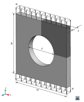
![Geometry (r=100 mm, h=w=200 mm, t=20 mm) and loading of the membrane with a hole as described in [Waffenschmidt2014] (left); and hexahedral mesh and boundary conditions imposed on the quarter of the membrane that has been discretized (right).](/wd/images/thumb/0/09/Draft_Samper_593843246-MeshMemb.png/270px-Draft_Samper_593843246-MeshMemb.png)

