A modified Taylor Galerkin scheme for turbulent compressible flow simulation.

Latest revision as of 14:25, 21 May 2021

Abstract

As already demonstrated by different authors, the Taylor-Galerkin (TG) scheme, in the context of the Finite Element Method (FEM), is particularly suitable for the solution of supersonic flows. The TG scheme, using hexahedral finite elements with analytical evaluation of element matrices, is applied in this work. Tools to avoid locking and a shock capturing technique for the solution of supersonic viscous and non-viscous compressible flows are also employed. However, TG scheme usually presents instabilities in subsonic flows. Even in cases in which the free stream Mach number corresponds to supersonic flows, there are always flow regions, specifically near the walls of the immersed obstacles, where the speed is lower, and the local Mach number corresponds to a subsonic flow. The Characteristic Based Split (CBS) scheme was developed in order to obtain a single method to improve the behavior with respect to TG method in subsonic and supersonic regimes. In the last two decades some works have shown advantages in convergence rates of the CBS method when compared to the TG algorithm. However, simulation time increases in the CBS method since split operations, typical of this algorithm, imply in additional element loops. In this paper a hybrid algorithm called Modified-Taylor-Galerkin scheme (MTG) is proposed. This algorithm presents advantages with respect to TG and CBS schemes in terms of convergence properties and computational processing time. In order to get an efficient algorithm, the element matrices are analytically integrated. This is performed with two different approaches. In the first approach the inverse matrix and the determinant of the Jacobian matrix at element level are evaluated with a reduced integration form, using the point located in the center of the element for mass, convective, diffusive and stabilization element matrices; all these matrices are integrated analytically. In the second approach, mass and convective matrices are calculated by a complete integration scheme (including the inverse matrix and the determinant of the Jacobian matrix at element level in the analytical expression to be integrated) and the diffusive and stabilization matrices are calculated with a reduced integration form, using the point located at the center of the element to calculate the inverse matrix and the determinant of the Jacobian matrix at element level. Finally, this work incorporates the Spalart-Allmaras (S-A) turbulence model using a conservative version of the transport equation, as proposed by the authors of the original S-A model in a later paper. Algorithms are tested to determine convergence rate improvements in both laminar and turbulent cases and for different Mach numbers (supersonic, transonic and subsonic flows).

Keywords: Compressible turbulent, FEM, Taylor-Galerkin, CBS, Spalart-Allmaras

1. Introduction

Different authors have shown that, in the context of FEM, the TG scheme is particularly suitable for the solution of compressible flows involving supersonic shock waves at high Mach numbers [1-2]. Burbridge and Awruch [3] applied this scheme using hexahedral finite elements with analytical evaluation of the element matrices but evaluating the inverse matrix and the determinant of the Jacobian matrix at the center of the element, together with a shock capturing technique for the solution of viscous and non-viscous compressible laminar flows [4]. However, for subsonic regimes (with M <0.9) or for incompressible flows, the TG scheme presents certain instabilities, as reported by Zienkiewicz and Taylor [5].

Even in supersonic flows there are always some regions of subsonic flow near the walls of immersed obstacles. It is therefore necessary to improve the convergence of the algorithms for low Mach numbers, even when they are applied to flows where Mach number at the freestream is supersonic.

To address this problem the CBS scheme was developed by some researchers, such as Zienkiewicz and Codina [6], to obtain a single algorithm with a good behavior, both in subsonic and supersonic regimes. During the last two and a half decades this algorithm was established as an acknowledged tool for the computation of a wide spectrum of incompressible or compressible flows at different Mach numbers [7-10]. The work presented by Zienkiewicz et al. in Reference [11] shows the explicit form of the algorithm and its performance for subsonic, transonic and supersonic flows.

However, in spite of convergence rates improvements, it is observed that computational processing time increases due to split operations involved in the CBS scheme. For this reason, an alternative hybrid algorithm is presented here, looking for improvements in convergence properties with respect to the TG algorithm without an increase of the computational processing time.

It is important to mention that, as in previous works [3,12], an analytical integration of the element matrices was used here, evaluating the inverse matrices and the determinants of the Jacobian matrices at the center of the element. But in this work, an alternative approach was also applied, integrating mass and convective matrices in an exact analytical form (including the inverse matrices and the determinants of the Jacobian matrices in the analytical expressions) using Maxima symbolic resolution program (http://maxima.sourceforge.net/). Stabilization and convective matrices were integrated in reduced form (evaluating the inverse matrices and the determinants of the Jacobian matrices at the center of the elements), as performed in [3,12].

Finally, the turbulence model of Spalart-Allmaras (S-A) was implemented here in order to test the behavior of these schemes, and their convergence properties, in the context of the FEM for turbulent flows. The form of the S-A model implemented here was proposed for the first time by Allmaras et al. [13] in 2012, using the transport equation for the turbulent modified kinematic viscosity variable ${\textstyle {\tilde {\nu }}}$ in conservative form.

TG, CBS and MTG schemes are presented here with some cases of laminar and turbulent flows, comparing their performances.

2. Governing equations with Spalart-Allmaras turbulence model

In an Eulerian description, the dimensionless system of partial differential equations governing the fluid dynamics problem in conservative form, and filtered with a Favre filter (FANS), may be written as follows:

(1)

where

{\boldsymbol {U}}=\left\{{\begin{matrix}\rho \\\rho {v}_{1}\\\rho {v}_{2}\\\rho {v}_{3}\\\rho e\\\rho {\tilde {\nu }}\end{matrix}}\right\};{\boldsymbol {F}}_{i=}\left\{{\begin{matrix}\rho {v}_{i}\\\rho {v}_{1}{v}_{i}+p{\delta }_{i1}\\\rho {v}_{2}{v}_{i}+p{\delta }_{i2}\\\rho {v}_{3}{v}_{i}+p{\delta }_{i3}\\{v}_{i}\left(\rho e+p\right)\\\rho {\tilde {\nu }}{v}_{i}\end{matrix}}\right\};{\boldsymbol {G}}_{i}=

(2)

The dimensionless form has been obtained using a reference length, the freestream density and the freestream speed of sound. In Eq. (2):

${\textstyle {v}_{i}\,}$ are velocity vector components.

${\textstyle \rho }$ is the specific mass.

${\textstyle p}$ is the thermodynamic pressure.

${\textstyle {\tau }_{ij}\,}$ are the viscous components of the stress tensor.

${\textstyle e}$ is the specific total energy.

${\textstyle {\tilde {\nu }}}$ is the transport equation variable of the S-A conservative turbulence model.

${\textstyle {q}_{i}}$ are the conduction heat flux vector components.

${\textstyle {\delta }_{ij}\,}$ is the Kronecker delta.

${\textstyle {\varphi }_{i}}$ is the diffusive term of the S-A transport equation.

${\textstyle {\psi }_{i}}$ is the diffusive term associated with turbulent kinetic energy ( ${\textstyle k}$ ) in the energy equation.

${\textstyle P}$ is the production term and D is the destruction term of the S-A transport equation.

${\textstyle {D}_{T}\,}$ contains additional terms of the S-A transport equation.

${\textstyle {x}_{i}\,}$ and t are the spatial and temporal coordinates, respectively.

${\textstyle i,j}$ =1,2,3.

The viscous stress components of a Newtonian fluid are given by:

(3)

where ${\textstyle \mu }$ and ${\textstyle {\mu }_{t}}$ are the molecular viscosity and the eddy viscosity, respectively, ${\textstyle k}$ is the turbulent kinetic energy and the subscript ${\textstyle k}$ runs from 1 to 3.

The components of the conduction heat flux vector are:

(4)

where ${\textstyle K}$ and ${\textstyle {K}_{t}}$ are the thermal conductivity and the turbulent thermal conductivity respectively and u is the specific internal energy.

The terms ${\textstyle {\psi }_{i}}$ in the energy equation are given by the following expression:

(5)

where ${\textstyle {\sigma }_{k}}$ is a constant which depends on the turbulence model. Since the S-A turbulence model does not include the calculation of turbulent kinetic energy, in this work, ${\textstyle {\psi }_{i}}$ in Eq. (2) and the third term in Eq. (3) are neglected.

The terms ${\textstyle {\varphi }_{i}}$ in the S-A transport equation are given by the following expression:

(6)

The transport equation also includes the additional term ${\textstyle {D}_{T}}$ , expressed by

(7)

where ${\textstyle \sigma }$ and ${\textstyle {cb}_{2}}$ are constants of the S-A turbulence model.

Finally, the production and destruction terms, in the conservative transport equation of S-A are given by

(8)

where the first term ${\textstyle P}$ represents the production and the second term D the destruction, being ${\textstyle {cb}_{1}}$ , ${\textstyle S}$ , ${\textstyle {cw}_{1}}$ and ${\textstyle {f}_{w}}$ constants and variables of the S-A turbulence model and ${\textstyle d}$ is the smallest distance from a field point (or node) to the nearest solid boundary (wall). The transport equation used here is expressed in its conservative form (Allmaras et al. [13]). Here the trip-term and the term of laminar suppression, both included in the original expressions of the model, are not considered.

To close the system of equations it is still necessary to define all parameters associated with the S-A turbulence model; they are given by

${\textstyle S=\Omega +\,{f}_{v2}\,{\frac {\tilde {\nu }}{{{\mathrm {K} }^{2}d}^{2}}}\,;\,\mathrm {K} =}$ $0.41$ ${\boldsymbol {\Omega }}=\,\,{\frac {1}{2}}\,rot{\mathit {\boldsymbol {V;\,}}}\Omega ={\sqrt {{\boldsymbol {\Omega }}\cdot {\boldsymbol {\Omega }}}}$

(9)

where ${\textstyle \Omega }$ is the magnitude of the angular velocity vector, and

${f}_{w}=g{\left({\frac {1+{{c}_{w3}}^{6}}{{g}^{6}+{{c}_{w3}}^{6}}}\right)}^{\frac {1}{6}}\,;\,{c}_{w3}=2.0\,;\,g=r+$ ${c}_{w2}\left({r}^{6}-r\right);\,{c}_{w2}=0.3$

$r={\frac {\tilde {\nu }}{{{S\,\mathrm {K} }^{2}d}^{2}}}\,;\,{c}_{w1}={\frac {{\,cb}_{1}}{{\mathrm {K} }^{2}}}+$ $\,{\frac {1+{\,cb}_{2}}{\sigma }}$

(10)

The turbulent viscosity and turbulent thermal conductivity are defined as follows:

(11)

where ${\textstyle {Pr}_{t}}$ is the turbulent Prandtl number, which is adopted as ${\textstyle {Pr}_{t}=}$ $0.9$ and ${\textstyle {c}_{v}\,}$ and ${\textstyle {c}_{p}\,}$ are the specific heat coefficients at constant volume and at constant pressure, respectively.

The state equation for a perfect gas (air) is given by:

(12)

The internal energy u and the temperature are related to the independent field variables by the following expression:

(13)

where ${\textstyle T}$ is the temperature, being ${\textstyle k}$ neglected in the S-A model.

The Sutherland law is used in this work to establish the dependence of viscosity and thermal conductivity with respect to temperature (dimensionless internal energy). This law can be expressed as follows:

(14)

Values of ${\textstyle S}$ and ${\textstyle {S}_{k}}$ may be found in reference [14] for the Sutherland law based on temperature; they must be multiplied by ${\textstyle {c}_{v}}$ and divided by the square of the freestream sound speed to obtain the dimensionless form, which was used in this work.

Initial and boundary conditions must be applied to Eq. (1) in order to obtain a mathematical model correctly defined. The forced boundary conditions (or Dirichlet boundary conditions) are given by:

{\begin{array}{ll}{v}_{i}={\overline {{v}_{i}}}\quad &{\hbox{on}}\quad {\Gamma }_{v}\\\rho ={\overline {\rho }}\quad &{\hbox{on}}\quad {\Gamma }_{\rho }\\u={\overline {u}}\quad &{\hbox{on}}\quad {\Gamma }_{u}\\{\tilde {\nu }}={\overline {\tilde {\nu }}}\quad &{\hbox{on}}\quad {\Gamma }_{\tilde {\nu }}\end{array}}

(15)

where ${\textstyle {\overline {{v}_{i}}}}$ , ${\textstyle {\overline {\rho }}\,,\,{\overline {u}}}$ and ${\textstyle {\overline {\tilde {\nu }}}}$ are prescribed values of the velocity vector components, the density (specific mass), the specific internal energy and the variable ${\textstyle {\tilde {\nu }}}$ , at the boundary surfaces ${\textstyle {\Gamma }_{v}}$ , ${\textstyle {\Gamma }_{\rho }}$ , ${\textstyle {\Gamma }_{u}}$ and Г ${\textstyle {\tilde {v}}\quad }$ respectively.

The natural boundary conditions (or Neumann boundary conditions) are defined by the following expressions:

(16)

In Eq. (16)

${\textstyle {n}_{i}\,}$ are the cosines of the angles formed by the normal vector to the surface ${\textstyle {\Gamma }_{\sigma }}$ or ${\textstyle {\Gamma }_{q}}$ and the global reference axes ${\textstyle {x}_{i}}$ .

${\textstyle {\hat {{t}_{i}}}\,}$ are the tractions acting on ${\textstyle {\Gamma }_{\sigma }}$ .

${\textstyle {\sigma }_{ij}\,=\,-p{\delta }_{ij}+\,{\tau }_{ij}}$ are the components of the Cauchy stress tensor.

${\textstyle {\hat {q}}\,}$ is the heat flow acting on the perpendicular direction to ${\textstyle \,{\Gamma }_{q}}$ .

Effects of thermal radiation on boundary surfaces have not been considered.

For non-viscous flows the transport equation of the variable ${\textstyle {\tilde {\nu }}}$ and the diffusive terms ${\textstyle {\boldsymbol {G}}_{i}}$ in Eq. (1) should be omitted. In this case, only normal velocity components to the solid boundaries are prescribed with null values and only the normal components of the surface tractions on the outlet boundaries are considered.

3. Finite element formulation

In this section the well-known TG, CBS and Single Step CBS algorithms are mentioned but the respective equations are not shown for the sake of brevity. The reader can look at the references [1,3,5,6,8] to get more details. Instead, the full matrix equations for the proposed MTG scheme are presented in the section 4.

3.1 Taylor-Galerkin (TG) scheme

To discretize Eq. (1) in time, the unknown vector ${\textstyle {\boldsymbol {U}}}$ is expanded in Taylor series omitting higher order terms. Then the space discretization is done using the classic Bubnov-Galerkin technique in the context of the finite element method. The Green-Gauss theorem is applied to terms containing second order derivatives (terms with third or higher order derivatives are neglected) to weaken the demands with respect to continuity of the element interpolation functions and their derivatives, obtaining the matrix equations [1-3].

A conditionally stable explicit time integration version of the TG scheme [4,5,15], may be obtained working with a lumped mass matrix (where only elements of the main diagonal are different from zero).

Also, it is important to point out that the increments of the flux variables obtained for the current time step ${\textstyle \,n+}$ $1\,$ with the TG scheme depend of flow variables at the previous time step ${\textstyle n\,}$ and at the current time step ${\textstyle \,n+}$ $1$ . So, an iterative scheme to solve terms involving flow variables at the new time step is required [1,3].

3.2 Characteristic Based Split (CBS) method

The CBS method consists of four steps [6]. In the first step, intermediate values of the conservative flow variables of the momentum equations are calculated, omitting the terms containing pressure gradients. In the second step, the continuity equation is solved to obtain the density increment. In the third step, the flow variables of the momentum equations are updated. In the fourth step, the energy equation and the S-A transport equation in its conservative form are solved. Finally, pressure is calculated using the state equation.

Once the temporal discretization is performed, spatial domain discretization is carried out using the classic Bubnov-Galerkin method. The Green-Gauss theorem is applied to terms containing second order derivatives to weaken the demands with respect to continuity of the element interpolation functions and their derivatives.

This method may be applied with implicit, semi-implicit and explicit time integration schemes [11]. An explicit scheme was implemented in this work in order to compare its behavior with respect to other explicit algorithms presented here.

Matrix expressions obtained with the CBS method may be found in references [5,6,8].

3.3 Single-Step CBS method

An alternative of the CBS method consists in the elimination of the split in the momentum equation in order to obtain a one-step algorithm. Some authors [5,6] suggest that, although the single-step CBS scheme saves computational processing time with respect to the classical CBS method, it is not suitable to simulate flows with high Mach numbers. The explicit version of the single-step CBS was implemented in this work. The common matrix expressions obtained with single-step CBS scheme can be found in reference [5].

4. The modified Taylor-Galerkin scheme

It may be observed that stabilization problems arise when TG scheme is used, and they are linked with density and pressure values, being these variables basically controlled by the continuity equation. The TG method is an efficient technique in terms of computational processing time, but schemes such as CBS have much better convergence properties for problems involving a wide range of Mach numbers. In order to link both features (computational efficiency and good convergence properties), a modification of the TG scheme is proposed. The new scheme is called Modified Taylor-Galerkin (MTG) scheme, which consists to change the stabilization term on the continuity equation by a similar expression, but defined in terms of pressure, as used in the CBS method. Since the TG scheme has good convergence rates for supersonic flows, the modification is only implemented in regions where the local Mach number is less than one. For this reason, a blending function ${\textstyle f}$ is proposed such that, the continuity equation discretized in time results:

{\begin{matrix}\Delta {\left(\rho \right)}_{I+1}^{n+1}=\Delta t\left\{-\displaystyle {\frac {{\partial \left({\rho v}_{i}\right)}^{n}}{{\partial x}_{i}}}+\displaystyle {\frac {\Delta t}{2}}\left[f{\frac {\partial }{{\partial x}_{i}}}\left(\displaystyle {\frac {{\partial p}^{n}}{{\partial x}_{i}}}\right)+\left(1-f\right)\displaystyle {\frac {\partial }{\partial {x}_{k}}}\left({{v}_{k}}^{n}\,\displaystyle {\frac {{\partial \left({\rho v}_{i}\right)}^{n}}{\partial {x}_{i}}}\right)\right]\right\}+\\\quad \quad \quad \quad \quad \quad \quad \quad \quad +\displaystyle {\frac {\Delta t}{2}}\left\{-\displaystyle {\frac {\partial \Delta {\left({\rho v}_{i}\right)}_{I}^{n+1}}{{\partial x}_{i}}}+\displaystyle {\frac {\Delta t}{2}}\left[f\displaystyle {\frac {\partial }{{\partial x}_{i}}}\left(\displaystyle {\frac {{\partial \Delta p}_{I}^{n+1}}{{\partial x}_{i}}}\right)+\left(1-f\right)\displaystyle {\frac {\partial }{\partial {x}_{k}}}\left({{v}_{k}}^{n}\,\displaystyle {\frac {{\partial \left(\Delta {\rho v}_{i}\right)}_{I}^{n+1}}{\partial {x}_{i}}}\right)\right]\right\}\end{matrix}}\,

(17)

where

(18)

The blending function ${\textstyle f}$ depends of the Mach number, which is evaluated locally. Momentum and energy equations as well as their iterative terms are not modified, remaining as in the original TG scheme.

Spatial discretization is performed using the classical Bubnov-Galerkin method. The Green-Gauss theorem is applied to terms containing second order derivatives to weaken the demands with respect to continuity of the element interpolation functions and their derivatives.

The following matrix expressions are obtained for the element vectors of independent unknowns’ increments:

Mass conservation equation:

{\begin{matrix}{\left.{\boldsymbol {\Delta \rho }}\right|}_{I+1}^{n+1}=f\left[{\Delta t}_{ext}\,{{\boldsymbol {M}}_{\boldsymbol {D}}}^{-1}\left(-{\boldsymbol {B}}_{i}\,{\left.{\boldsymbol {f}}_{i}^{\rho }\right|}^{n}-{\boldsymbol {P}}{\boldsymbol {\,p}}^{n}-{\boldsymbol {r}}^{n}\right)+\displaystyle {\frac {{\Delta t}_{ext}}{2}}{{\boldsymbol {M}}_{\boldsymbol {D}}}^{-1}\left(-\,{\boldsymbol {B}}_{i}\,{\left.{\boldsymbol {\Delta f}}_{i}^{\rho }\right|}_{I}^{n+1}-{\boldsymbol {P}}\,{\boldsymbol {\Delta p}}_{I}^{n+1}\right)\right]+\\\quad \quad \quad +\left(1-f\right)\left[{\Delta t}_{ext}{{\boldsymbol {M}}_{\boldsymbol {D}}}^{-1}\left(-{\boldsymbol {H}}_{i}\,{\left.{\boldsymbol {f}}_{i}^{\rho }\right|}^{n}\right)+\displaystyle {\frac {{\Delta t}_{ext}}{2}}{{\boldsymbol {M}}_{\boldsymbol {D}}}^{-1}\left(-\,{\boldsymbol {H}}_{i}\,{\left.{\boldsymbol {\Delta f}}_{i}^{\rho }\right|}_{I}^{n+1}\right)\right]\end{matrix}}

(19a)

Momentum conservation equations:

\quad {\begin{matrix}{\left.{\boldsymbol {\Delta \rho }}{\boldsymbol {v}}_{j}\right|}_{I+1}^{n+1}={\Delta t}_{ext}\,{{\boldsymbol {M}}_{\boldsymbol {D}}}^{-1}\left(-\,{\boldsymbol {H}}_{i}\,{\left.{\boldsymbol {f}}_{ij}^{\rho v}\right|}^{n}-{\boldsymbol {D}}_{ij}{{\boldsymbol {\,v}}_{i}}^{n}+{{\boldsymbol {t}}_{j}}^{n}\right)+\\\quad \quad \quad \quad \,+\displaystyle {\frac {{\Delta t}_{ext}}{2}}{{\boldsymbol {M}}_{\boldsymbol {D}}}^{-1}\left(-{\boldsymbol {H}}_{i}\,{\boldsymbol {\Delta }}{\left.{\boldsymbol {f}}_{ij}^{\rho v}\right|}_{I}^{n+1}-{\boldsymbol {D}}_{ij}{\left.{\boldsymbol {\,\Delta v}}_{i}\right|}_{I}^{n+1}\right)\end{matrix}}

(19b)

Energy conservation equation:

\,{\begin{matrix}{\left.{\boldsymbol {\Delta \rho e}}\right|}_{I+1}^{n+1}={\Delta t}_{ext}{{\boldsymbol {\,M}}_{\boldsymbol {D}}}^{-1}\left(-{\boldsymbol {H}}_{i}\,{\left.{\boldsymbol {f}}_{i}^{\rho e}\right|}^{n}-{\boldsymbol {E}}_{i}\,{{\boldsymbol {v}}_{i}}^{n}-{\boldsymbol {K}}\,{\boldsymbol {u}}^{n}+{\boldsymbol {h}}^{n}\right)+\\\quad \quad \quad \quad \quad \quad +\displaystyle {\frac {{\Delta t}_{ext}}{2}}{{\boldsymbol {M}}_{\boldsymbol {D}}}^{-1}\left(-{\boldsymbol {H}}_{i}\,{\left.{\boldsymbol {\Delta f}}_{i}^{\rho e}\right|}_{I}^{n+1}-{\boldsymbol {E}}_{i}\,{\left.{\boldsymbol {\Delta v}}_{i}\right|}_{I}^{n+1}-{\boldsymbol {K\,}}{\left.{\boldsymbol {\Delta u}}\right|}_{I}^{n+1}\right)\end{matrix}}

(19c)

Transport equation of ${\textstyle {\tilde {\nu }}}$ (being ${\textstyle {\tilde {\nu }}}$ a variable used in the S-A model):

{\begin{matrix}{\left.{\boldsymbol {\Delta \rho }}{\tilde {\boldsymbol {\nu }}}\right|}_{I+1}^{n+1}=\,{\Delta t}_{ext}{{\boldsymbol {\,M}}_{\boldsymbol {D}}}^{-1}\left(-{\boldsymbol {H}}_{i}\,{\left.{\boldsymbol {f}}_{i}^{\rho {\tilde {\nu }}}\right|}^{n}{\boldsymbol {-M}}\,{\boldsymbol {q}}^{n}-{\boldsymbol {A}}_{i}\,{\left.{\boldsymbol {q}}_{{\mathit {\boldsymbol {v}}}_{\mathit {\boldsymbol {i}}}}\right|}^{n}-{\boldsymbol {D}}_{\nu }\,{\tilde {\boldsymbol {\nu }}}^{n}\right)+\\\quad \quad \quad \quad \quad +\,\displaystyle {\frac {{\Delta t}_{ext}}{2}}{{\boldsymbol {M}}_{\boldsymbol {D}}}^{-1}\left(-{\boldsymbol {H}}_{i}\,{\left.{\boldsymbol {\Delta f}}_{i}^{\rho {\tilde {\nu }}}\right|}_{I}^{n+1}-{\boldsymbol {M}}\,{\boldsymbol {\Delta q}}_{I}^{n+1}-\,{\boldsymbol {D}}_{\nu }\,{\boldsymbol {\Delta }}{\tilde {\boldsymbol {\nu }}}_{I}^{n+1}\right)\end{matrix}}\quad \,\,

(19d)

An iteration procedure is required for those right-hand terms evaluated on the current time step ${\textstyle n+}$ $1$ , where the subscript ${\textstyle I}$ indicates the previous iteration and ${\textstyle I+}$ $1$ corresponds to the current one. Element matrices are indicated below (with ${\textstyle i,j,k=}$ $1,2,3$ ):

{\boldsymbol {B}}_{i}=\int _{{\Omega }_{E}}^{}{\boldsymbol {\phi }}^{T}\,{\frac {\partial {\boldsymbol {\phi }}}{\partial {x}_{i}}}\,d\Omega ;\quad {\boldsymbol {C}}_{i}={\frac {{\Delta t}_{in}}{2}}\int _{{\Omega }_{E}}^{}\left({\boldsymbol {\phi }}{{\boldsymbol {v}}_{k}}^{n}\right){\frac {\partial {\boldsymbol {\phi }}^{T}}{\partial {x}_{k}}}\,\displaystyle {\frac {\partial {\boldsymbol {\phi }}}{\partial {x}_{i}}}\,d\Omega ;\,\,{\boldsymbol {P}}=

$\,{\boldsymbol {H}}_{i}={\boldsymbol {B}}_{i}+{\boldsymbol {C}}_{i};\quad {\boldsymbol {A}}_{i}=$ ${\frac {{\Delta t}_{in}}{2}}{\boldsymbol {B}}_{i}\,$

${\boldsymbol {D}}_{ij}=\left\{{\begin{matrix}\int _{{\Omega }_{E}}^{}\eta \left(2+\displaystyle {\frac {\lambda }{\eta }}\right)\displaystyle {\frac {\partial {\boldsymbol {\phi }}^{T}}{\partial {x}_{i}}}\displaystyle {\frac {\partial {\boldsymbol {\phi }}}{\partial {x}_{(i)}}}d\Omega +\int _{{\Omega }_{E}}^{}\eta \displaystyle {\frac {\partial {\boldsymbol {\phi }}^{T}}{\partial {x}_{k}}}\displaystyle {\frac {\partial {\boldsymbol {\phi }}}{\partial {x}_{k}}}d\Omega ,\,\,if\,i=j\qquad \quad {\hbox{and }}\quad \left\{{\begin{matrix}i=1\rightarrow k=2,3\\i=2\rightarrow k=1,3\\i=3\rightarrow k=1,2\end{matrix}}\right.\,\,\\\int _{{\Omega }_{E}}^{}\eta \displaystyle {\frac {\partial {\boldsymbol {\phi }}^{T}}{\partial {x}_{i}}}\,\displaystyle {\frac {\partial {\boldsymbol {\phi }}}{\partial {x}_{j}}}\,d\Omega +\int _{{\Omega }_{E}}^{}\lambda \displaystyle {\frac {\partial {\boldsymbol {\phi }}^{T}}{\partial {x}_{j}}}\,\displaystyle {\frac {\partial {\boldsymbol {\phi }}}{\partial {x}_{i}}}\,d\Omega ,\quad \quad \quad \quad \quad \quad \quad \quad \quad \quad {\hbox{if}}\quad \,i\,\not =j\end{matrix}}\right.$

$\eta ={\mu +\mu }_{t};\,\lambda =-{\frac {2}{3}}\eta$

${\boldsymbol {E}}_{i}=\int _{{\Omega }_{E}}^{}\left[\eta \left({\boldsymbol {\phi }}{{\boldsymbol {\,v}}_{i}}^{n}\right)\,{\frac {\partial {\boldsymbol {\phi }}^{T}}{\partial {x}_{k}}}\,{\frac {\partial {\boldsymbol {\phi }}}{\partial {x}_{k}}}+\eta \left({\boldsymbol {\phi \,}}{{\boldsymbol {v}}_{k}}^{n}\right)\,{\frac {\partial {\boldsymbol {\phi }}^{T}}{\partial {x}_{i}}}\,{\frac {\partial {\boldsymbol {\phi }}}{\partial {x}_{k}}}\right]d\Omega +$ $\int _{{\Omega }_{E}}^{}\lambda \left({\boldsymbol {\phi }}{{\boldsymbol {\,v}}_{k}}^{n}\right)\,{\frac {\partial {\boldsymbol {\phi }}^{T}}{\partial {x}_{k}}}\,{\frac {\partial {\boldsymbol {\phi }}}{\partial {x}_{i}}}\,d\Omega$

${\boldsymbol {K}}=\int _{{\Omega }_{E}}^{}\left({K+K}_{t}\right){\frac {\partial {\boldsymbol {\phi }}^{T}}{\partial {x}_{i}}}\,{\frac {\partial {\boldsymbol {\phi }}}{\partial {x}_{i}}}\,d\Omega ;\quad {\boldsymbol {D}}_{\nu }=$ $\int _{{\Omega }_{E}}^{}{\frac {1}{\sigma }}\left[\mu +\left({\boldsymbol {\phi }}{\left\{\rho \nu \right\}}^{n}\right)\right]{\frac {\partial {\boldsymbol {\phi }}^{T}}{\partial {x}_{i}}}{\frac {\partial {\boldsymbol {\phi }}}{\partial {x}_{i}}}\,d\Omega$

${\boldsymbol {M}}=\int _{{\Omega }_{E}}^{}{\boldsymbol {\phi }}^{T}{\boldsymbol {\phi }}d\Omega ;\,\,{\boldsymbol {M}}_{\boldsymbol {D}}=$ $\left\{{\begin{array}{cl}{\frac {{\Omega }_{E}}{8}}\quad \quad &{\hbox{for diagonal terms.}}\,\\\\0\quad \quad &{\hbox{off-diagonal terms.}}\end{array}}\right.$

(20a)

The element vectors are:

${\begin{matrix}\displaystyle {\boldsymbol {q}}^{n}=-{cb}_{1}\,{{S}_{E}}^{n}\,{\left\{\rho {\tilde {\nu }}\right\}}^{n}+{cw}_{1}\,{{{f}_{w}}_{E}}^{n}\,{\left\{\rho \,{\left(\displaystyle {\frac {\tilde {\nu }}{d}}\right)}^{2}\right\}}^{n}-\displaystyle {\frac {{cb}_{2}}{\sigma }}\,{\left({\rho }_{E}\,{\left.\displaystyle {\frac {\partial {\tilde {\nu }}}{\partial {x}_{i}}}\right|}_{E}{\left.\displaystyle {\frac {\partial {\tilde {\nu }}}{\partial {x}_{i}}}\right|}_{E}\right)}^{n}\left\{1\right\}+\\\displaystyle +\,\displaystyle {\frac {1}{\sigma }}{\left[\left({\nu }_{E}+{\tilde {\nu }}_{E}\right){\left.\displaystyle {\frac {\partial \rho }{\partial {x}_{i}}}\right|}_{E}{\left.\displaystyle {\frac {\partial {\tilde {\nu }}}{\partial {x}_{i}}}\right|}_{E}\right]}^{n}\left\{1\right\}\end{matrix}}$

${\begin{matrix}{\left.\displaystyle {\boldsymbol {q}}_{{\mathit {\boldsymbol {v}}}_{\mathit {\boldsymbol {i}}}}\right|}^{n}=-{cb}_{1}\,{{S}_{E}}^{n}\,{\left\{\rho {\tilde {\nu }}{v}_{i}\right\}}^{n}+{cw}_{1}\,{{{f}_{w}}_{E}}^{n}\,{\left\{\rho \,{\left(\displaystyle {\frac {\tilde {\nu }}{d}}\right)}^{2}{v}_{i}\right\}}^{n}-\displaystyle {\frac {{cb}_{2}}{\sigma }}\,{\left({\rho }_{E}\,{\left.\displaystyle {\frac {\partial {\tilde {\nu }}}{\partial {x}_{i}}}\right|}_{E}{\left.\displaystyle {\frac {\partial {\tilde {\nu }}}{\partial {x}_{i}}}\right|}_{E}\right)}^{n}{{\boldsymbol {v}}_{i}}^{n}+\\\displaystyle +\,\displaystyle {\frac {1}{\sigma }}{\left[\left({\nu }_{E}+{\tilde {\nu }}_{E}\right){\left.\displaystyle {\frac {\partial \rho }{\partial {x}_{i}}}\right|}_{E}{\left.\displaystyle {\frac {\partial {\tilde {\nu }}}{\partial {x}_{i}}}\right|}_{E}\right]}^{n}{{\boldsymbol {v}}_{i}}^{n}\end{matrix}}$

(20b)

where ${\textstyle \,{\boldsymbol {v}}_{i}=\left\{{v}_{i}\right\}}$ , ${\textstyle {\boldsymbol {p}}=}$ $\left\{p\right\}{\boldsymbol {,\,}}{\boldsymbol {u}}=\left\{u\right\}$ are ${\textstyle \,}$ the velocity components, pressure and internal energy element vectors, containing their corresponding eight nodal values. The quantities between braces are element vectors built with the nodal values of the variables inside the braces. The boundary vectors are:

$\displaystyle {{\boldsymbol {t}}_{j}}^{n}=\int _{{\Gamma }_{E}}^{}{{\boldsymbol {\phi }}^{\ast }}^{T}\,\left[\eta \,\left({\frac {\partial {\boldsymbol {\phi }}}{\partial {x}_{i}}}\,{{\boldsymbol {v}}_{j}}^{n}+{\frac {\partial {\boldsymbol {\phi }}}{\partial {x}_{j}}}{{\boldsymbol {v}}_{i}}^{n}\right)+\,\lambda \,\left({\frac {\partial {\boldsymbol {\phi }}}{\partial {x}_{k}}}\,{{\boldsymbol {v}}_{k}}^{n}\right){\delta }_{ij}\right]{n}_{i}\,\,d\Gamma$

${\begin{matrix}\displaystyle {\boldsymbol {h}}^{n}={\displaystyle \int }_{{\Gamma }_{E}}^{}{{\boldsymbol {\phi }}^{\ast }}^{T}\,\left({\boldsymbol {\phi }}{{\boldsymbol {\,v}}_{j}}^{n}\right)\left[\eta \left(\displaystyle {\frac {\partial {\boldsymbol {\phi }}}{\partial {x}_{i}}}\,{{\boldsymbol {v}}_{j}}^{n}+\displaystyle {\frac {\partial {\boldsymbol {\phi }}}{\partial {x}_{j}}}{{\boldsymbol {v}}_{i}}^{n}\right)+\lambda \left(\displaystyle {\frac {\partial {\boldsymbol {\phi }}}{\partial {x}_{k}}}\,{{\boldsymbol {v}}_{k}}^{n}\right){\delta }_{ij}\right]{n}_{i}\,\,d\Gamma +\\\displaystyle +\,{\displaystyle \int }_{{\Gamma }_{E}}^{}{{\boldsymbol {\phi }}^{\ast }}^{T}\,\left({K+K}_{t}\right)\,\left(\displaystyle {\frac {\partial {\boldsymbol {\phi }}}{\partial {x}_{i}}}{\boldsymbol {u}}^{n}\right)\,{n}_{i}\,\,d\Gamma \end{matrix}}$

(20c)

In these expressions ${\textstyle {\Omega }_{E}}$ and ${\textstyle {\Gamma }_{E}}$ are the element volume and its boundary surface respectively; expressions with the subscript ${\textstyle E}$ are element averages; ${\textstyle {\boldsymbol {\phi }}}$ = [Ф₁, Ф₂_{, …} Ф₈] is the row matrix containing the interpolation functions for each local node and ${\textstyle {\boldsymbol {\phi }}^{\ast }}$ is the row matrix containing the interpolation functions evaluated at the boundary surface, ${\textstyle {\boldsymbol {M}}}$ is the consistent mass matrix, while ${\textstyle {\boldsymbol {M}}_{\boldsymbol {D}}}$ is the lumped mass matrix and ${\textstyle \left\{1\right\}}$ is a vector where all its components are equal to one. Terms that involve turbulent kinetic energy have been neglected.

The variables with superscript ${\textstyle n}$ are evaluated on previous time step and the variables with superscript ${\textstyle n+}$ $1$ are evaluated at current time step. Boundary vectors appearing in the S-A transport equation and in the iterative terms of all the equations were neglected.

Once these equations are assembled for all the elements of the mesh and the corresponding boundary conditions are applied, the nodal values of ${\textstyle \rho }$ , ${\textstyle \rho {v}_{j}}$ ${\textstyle \rho e}$ and ${\textstyle \rho {\tilde {\nu }}}$ can be calculated at each time step using an iterative scheme. Thus, the nodal values of the components of velocity, the specific total energy and the variable ${\textstyle {\tilde {\nu }}}$ can be obtained immediately. Then the nodal values of the specific internal energy are calculated and, using the state equation, the nodal pressure values are also obtained.

When viscous terms are not considered, terms containing matrices ${\textstyle {\boldsymbol {D}}_{ij}}$ , ${\textstyle {\boldsymbol {E}}_{i}}$ and ${\textstyle {\boldsymbol {K}}}$ as well as vectors ${\textstyle {{\boldsymbol {t}}_{j}}^{n}}$ and ${\textstyle {\boldsymbol {h}}^{n}}$ and the transport equation corresponding to the turbulence model are omitted.

Stabilization matrices for TG, CBS and MTG schemes are evaluated using a local (internal) time step ${\textstyle {\Delta t}_{in}}$ . For the TG scheme there are no appreciable differences in using a local internal time step or a single time step ${\textstyle {\Delta t}_{ext}}$ [16].

5. Stability condition, shock capture and convergence

Considering that these algorithms were implemented in their explicit form, they are conditionally stable and the stability condition of Courant-Friedrichs-Lewy (CFL) for each element, in dimensionless form, is used to ensure stability. A safety coefficient ${\textstyle \beta }$ is adopted with values ${\textstyle 0.2\leq \beta \leq \,0.5}$ [3].

To capture the strong discontinuities and eliminate high frequency oscillations near shock waves, a well-known method is used to add artificial viscosity selectively in regions where high-pressure gradients are observed [17]. An artificial damping coefficient ${\textstyle {C}_{AD}}$ is used to control de amount of artificial viscosity.

The convergence of the iterative process is obtained when the following conditions are simultaneously satisfied:

${r}_{I+1}^{\rho v}={\left[{\frac {\sum _{N}^{}{\left|{\rho v}_{iI+1}-{\rho v}_{iI}\right|}^{2}}{\sum _{N}^{}{{\rho v}_{iI}}^{2}}}\right]}^{\frac {1}{2}}\leq To$

${r}_{I+1}^{\rho e}={\left[{\frac {\sum _{N}^{}{\left|{\rho e}_{I+1}-{\rho e}_{I}\right|}^{2}}{\sum _{N}^{}{{\rho e}_{I}}^{2}}}\right]}^{\frac {1}{2}}\leq To$

(21)

where ${\textstyle N}$ is an index of nodes ( ${\textstyle N=}$ $1,2,3,\ldots ,NNODES$ ), ${\textstyle NNODES}$ is the total number of nodes of the finite element mesh and ${\textstyle To}$ is the tolerance (in this paper ${\textstyle To=}$ ${10}^{-3}$ was adopted). The solution process ends when the variable ${\textstyle t}$ (time) reaches a value previously established by the user, or when the steady state is reached. This last condition is considered fulfilled when the following expression is satisfied:

(22)

In this work ${\textstyle TO{L}_{t}={10}^{-5}}$ was adopted.

6. Explicit integration of element matrices

Eight nodes isoparametric hexahedral elements were used in this work. Figures 1 and 2 show the element in the physical and computational spaces, respectively. The interpolation functions of this element are given by the following expressions:

(23)

where ${\textstyle N=1,2,3,\ldots ,8}$ and ${\textstyle {\xi }_{jN}}$ are the natural coordinates of the node ${\textstyle N}$ . The derivatives of the interpolation functions with respect to the global coordinates are given by:

(24)

being ${\textstyle {I}_{ij}^{-1}}$ the components of the inverse of the Jacobian matrix ${\textstyle {\mathit {\boldsymbol {\,}}}{\mathit {\boldsymbol {I}}}}$ , which can be expressed as follows:

{\mathit {\boldsymbol {I}}}\left({\xi }_{1},{\xi }_{2},{\xi }_{3}\right)=\left[{\begin{matrix}{I}_{11}\,{I}_{12}\,\,{I}_{13}\\{I}_{21}\,\,{I}_{22}\,\,{I}_{23}\\{I}_{31}\,\,{I}_{32}\,\,{I}_{33}\end{matrix}}\right]=

\left[{\begin{matrix}\displaystyle {\frac {\partial {\boldsymbol {\phi }}}{\partial {\xi }_{1}}}{\boldsymbol {x}}_{1}\,\,\displaystyle {\frac {\partial {\boldsymbol {\phi }}}{\partial {\xi }_{1}}}{\boldsymbol {x}}_{2}\,\,\displaystyle {\frac {\partial {\boldsymbol {\phi }}}{\partial {\xi }_{1}}}{\boldsymbol {x}}_{3}\\\displaystyle {\frac {\partial {\boldsymbol {\phi }}}{\partial {\xi }_{2}}}{\boldsymbol {x}}_{1}\,\,\displaystyle {\frac {\partial {\boldsymbol {\phi }}}{\partial {\xi }_{2}}}{\boldsymbol {x}}_{2}\,\,\displaystyle {\frac {\partial {\boldsymbol {\phi }}}{\partial {\xi }_{2}}}{\boldsymbol {x}}_{3}\\\displaystyle {\frac {\partial {\boldsymbol {\phi }}}{\partial {\xi }_{3}}}{\boldsymbol {x}}_{1}\,\,\displaystyle {\frac {\partial {\boldsymbol {\phi }}}{\partial {\xi }_{3}}}{\boldsymbol {x}}_{2}\,\,\displaystyle {\frac {\partial {\boldsymbol {\phi }}}{\partial {\xi }_{3}}}{\boldsymbol {x}}_{3}\end{matrix}}\right]

(25)

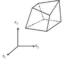
Figure 1. Physical space

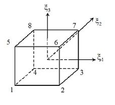
Figure 2. Computational space

Here ${\textstyle {\boldsymbol {x}}_{i}}$ is the vector containing global coordinates of the eight nodes of each element, ${\textstyle \,\left|{\mathit {\boldsymbol {I}}}\right|}$ is the determinant of the Jacobian matrix and ${\textstyle d\Omega =}$ $\left|{\mathit {\boldsymbol {I}}}\right|\,d{\xi }_{1}\,d{\xi }_{2\,}\,d{\xi }_{3\,}$ is the differential of the element volume.

By substituting Eqs. (23), (24) and (25) on the element matrices and vectors defined by the TG, CBS and MTG schemes, integrals in the computational domain are obtained. These integrals are commonly calculated by means of a numerical integration scheme to obtain components of the element matrices that will be later assembled to get the global system of equations. However, in this work, matrices were calculated by means of analytical integration using the Maxima symbolic resolution software. This implies an improvement in computational processing time efficiency.

In a first approach the inverse matrix elements and determinants of the Jacobian matrix were evaluated at the center of the element, where ${\textstyle {\xi }_{1}=}$ $\,{\xi }_{2\,}=\,{\xi }_{3\,}=0,$ and these values were used to integrate matrices corresponding to variables time derivatives, convective, diffusive and stabilization terms [3,12]. Special attention must be given to elements distortion and an hourglass control technique to avoid spurious modes on diffusive terms are also necessary [12].

Alternatively, in a second approach, the mass matrix ${\textstyle {\boldsymbol {\,}}{\boldsymbol {M}}}$ (representing variables time derivatives) and matrix ${\textstyle {\boldsymbol {B}}_{i}}$ (representing convective terms) were integrated analytically, including the inverse matrix elements and determinant of the Jacobian matrix in the analytical expressions (without evaluating these terms at the center of the element). However, to integrate matrices corresponding to stabilization and diffusive terms, the procedure used in the first approach was followed (inverse matrix elements and determinants of the Jacobian matrix were evaluated at the center of the element). Both integration approaches were used for the implementation of TG, CBS and MTG schemes.

7. Numerical simulations and comparative results

7.1 Transonic flow around a NACA 0012 airfoil

The laminar transonic flow around a NACA 0012 airfoil with ${\textstyle M=}$ $0.85\,$ and ${\textstyle Re=2000\,}$ is analyzed. Results obtained with version 17.1 of ANSYS/Fluent are compared with those obtained with the MTG scheme for the same problem. All simulations performed for this case were obtained with TG, MTG and CBS schemes with the second integration approach, that is, a complete analytical integration (including inverse matrix and determinant of the Jacobian matrix in the expressions to be evaluated analytically) for the mass and convective matrices, while the inverse matrix and determinant of the Jacobian matrix were evaluated at the center of the elements for the stabilization and diffusive matrices.

This problem is described with dimensionless quantities. The mesh used to solve this problem with 386 560 hexahedral elements and 775 684 nodes is shown in Figure 3. The coordinates axis are ${\textstyle x=}$ ${x}_{1}$ and ${\textstyle y={x}_{2}}$ . Figures 4 and 5 show details of the finite element mesh. It is considered as being three-dimensional mesh with a single element in the ${\textstyle z=}$ ${x}_{3}$ direction. The same mesh is used to run this problem with ANSYS/Fluent.

Considering that the mesh is three-dimensional with a single element in the ${\textstyle {x}_{3}}$ direction, the ${\textstyle \,{v}_{3}=}$ $0.0$ condition is imposed on the lateral boundaries to avoid mass flow through those boundaries, ensuring the two-dimensional characteristic of the flow.

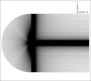
Figure 3. Side view of whole domain and the finite element mesh

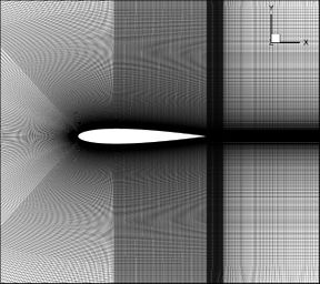
Figure 4. Side view of the mesh

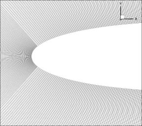
Figure 5. Details of the airfoil leading edge

The dimensionless inlet boundary conditions are:

;

On the solid boundaries the non-slip condition is applied. Then, on the airfoil wall:

together with the stagnation temperature, which is specified using the specific internal energy, according to the following expression:

where ${\textstyle r=0.89}$ is the recovery factor (an empirical factor introduced because in practice the energy recovery is not perfect [14]). The conditions at the output boundaries are specified using the vectors ${\textstyle {\boldsymbol {t}}_{j}}$ and ${\textstyle {\boldsymbol {q}}}$ .

Initial conditions are given by:

;

y

These initial conditions are defined for all nodes of the finite element mesh, excepting those where Dirichlet boundary conditions are prescribed.

Using the safety coefficient ${\textstyle \beta =0.2}$ , the effective dimensionless time step is ${\textstyle \Delta t=}$ ${0.5}^{\ast }{10}^{-4}$ . Artificial viscosity is not applied for this case ${\textstyle ({C}_{AD}=}$ $0.0)$ .

Figure 6 shows pressure contours obtained with the MTG scheme. Pressure contours obtained with CBS scheme are practically coincident with results obtained with MTG scheme and are not shown here. Figure 7 shows pressure contours obtained with ANSYS/Fluent 17.1 available at the GFC (Grupo de Fluidodinámica Computacional) of the UNLP (Universidad Nacional de La Plata). An excellent agreement was obtained between MTG and ANSYS/Fluent simulations. Figure 8 shows details of pressure contours at the leading edge of the airfoil obtained with the MTG scheme (CBS shows no appreciable difference). Figure 9 shows the same image, but obtained with the TG scheme, where pressure oscillations in zones of low air speeds can be observed. CBS and MTG schemes do not present these oscillations.

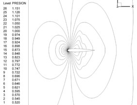
Figure 6. MTG pressure contours

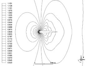
Figure 7. ANSYS / Fluent pressure contours

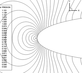
Figure 8. MTG pressure contours

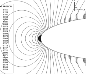
Figure 9. TG pressure contours

Figure 10 shows an image of the skin friction coefficient comparing the MTG scheme with values obtained with ANSYS/Fluent 17.1 showing a good agreement. Figure 11 shows the comparison of pressure coefficient obtained with ANSYS/Fluent 17.1 and the MTG scheme on the NACA 0012 airfoil extrados.

Here, the skin friction coefficient ${\textstyle {c}_{f}}$ and the pressure coefficient ${\textstyle {c}_{p}}$ were calculated using the following expressions:

where ${\textstyle \tau }$ is the wall tangent stress and ${\textstyle p}$ is the pressure, both acting on each point of the solid boundary surface.

Results obtained for these coefficients with MTG scheme applying an internal time step are very close to values obtained with ANSYS/Fluent 17.1.

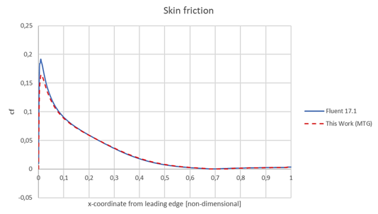
Figure 10. Skin friction coefficient over the airfoil extrados surface

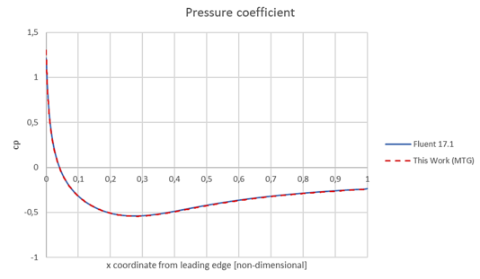
Figure 11. Pressure coefficient over the airfoil extrados surface

Figure 12 shows the convergence of the different schemes. The CBS method presents a clear improvement in density and pressure convergence when used with a local interior time step [16]. The use of an internal time step with the original TG method does not show comparative advantage with respect to the same method but taking a single time step. Notably, the performance of the MTG scheme with a local internal time step, is equivalent to that obtained with the CBS algorithm with a local internal time step.

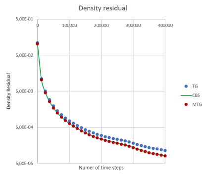
Figure 12. Residues showing convergence of the different algorithms

Additional simulations were carried out with the single-step CBS method. Results are not shown here, but they do not show significant differences compared to those obtained with the CBS or MTG schemes.

Relative times for the different simulations are indicated in Table 1, assuming a reference time with a value equal to one for the fastest scheme (the single-step CBS).

Table 1. Relative wall clock times

Algorithm	Relative wall clock time
Single-step CBS	1.0
TG	1.01
MTG	1.04
CBS	1.37

It should be noted that the cases shown in Table 1 correspond to simulations of the same problem, with the same mesh and boundary conditions, on the same computer (Dell Precision 7610, 16 Cores, 64 Gb ram), and using the same number of threads (16) in parallel. The times that are compared are wall clock times between two recordings of results with the same number of time steps. This problem was also solved using the first integration approach, that is, analytical integration with evaluation of the inverse matrices and determinants of the Jacobian matrices at the center of the elements for all the mass, convective, stabilization and diffusive matrices. There are not significant differences between both integration approaches.

It should also be pointed out that the codes for the different schemes were developed starting from the same original TG MPI parallel code, including only those modifications required by CBS, single-step CBS and MTG schemes. This ensures that the code structure is basically the same, with smallest differences required by the different algorithms.

7.2 Turbulent supersonic flow on flat plate

The turbulent compressible flow on a flat plate in supersonic regime with ${\textstyle M=}$ $2.0\,$ and ${\textstyle Re=15\ast {10}^{6}\,}$ is presented.

This problem is described at the NASA Langley Research Center Turbulence Modeling Resource on the web (https://turbmodels.larc.nasa.gov/), where results are shown for several turbulence models and they are compared with the semi-empirical theoretical correlations of Van Driest.

The geometry of this problem is shown in Figure 13. Considering that the mesh is three-dimensional with a single element in the ${\textstyle {x}_{2}}$ direction, the condition ${\textstyle {v}_{2}=}$ $0.0$ is imposed on the lateral boundaries to avoid the mass flow through them, keeping the two-dimensional characteristic of the flow.

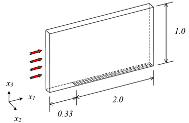
Figure 13. 3D view and geometric characteristics

Figure 14 shows the side view of the finite element mesh, which has 13 056 hexahedral elements and 26 578 nodes. The mesh is the same found in the NASA web repository for turbulence models (3-D with $2\times 137\times 97$ nodes and $2\times 113$ points on the flat plate).

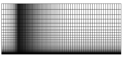
Figure 14. Side view of the mesh

The mesh was refined near the wall such that the estimate of ${\textstyle {y}^{+}}$ is close to 0.3.

The boundary conditions at the inlet are:

;

On the solid boundaries (over the plate) the non-slip condition is applied:

and

together with the stagnation temperature, which is specified using the specific internal energy, according to the following expression:

with ${\textstyle r=0.89}$ . The conditions in the output boundary are specified using the vectors ${\textstyle {\boldsymbol {t}}_{j}}$ and ${\textstyle {\boldsymbol {q}}}$ . The initial conditions are given by:

;

y

These initial values are defined in all nodes of the mesh, except for the nodes where Dirichlet boundary conditions were prescribed.

Using the safety factor ${\textstyle \beta =0.2}$ , the dimensionless time step is ${\textstyle \Delta t=}$ ${1.0}^{\ast }{10}^{-7}$ . The artificial viscosity coefficient used here is ${\textstyle {C}_{AD}=}$ $0.3$ .

The pressure contours obtained with the TG, MTG and CBS schemes shown no appreciable differences. However, the researchers who developed the CBS scheme [6] point out that the single-step CBS scheme is not suitable for high Mach numbers. The simulations carried out in this work with this scheme for high Mach numbers indicate that the convergence of the single-step CBS presents some instabilities. Therefore, observations given in the reference [6] is confirmed here: single-step CBS scheme is not recommended for supersonic flows.

In Figure 15 an image of the skin friction coefficient, comparing with values provided by the semi-empirical correlation of Van Driest II (see the NASA Langley Research Center Turbulence Modeling Resource) is shown. Good agreement is observed. There are no appreciable differences between results obtained with different schemes (TG, CBS and MTG). All these schemes seem to be adequate in terms of quality of the results.

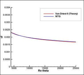
Figure 15. Skin friction coefficient over the plate

Finally, Figure 16 shows the dimensionless velocity profile, corresponding to the position of the plate where ${\textstyle {Re}_{\theta }=}$ $10\,000$ . As can be observed, results obtained in this work are very close to values shown at the NASA repository for the velocity profile, corresponding to the semi-empirical correlation of Van Driest I.

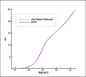
Figure 16. Velocity profile at

The convergence between the TG, MTG and CBS schemes does not differ significantly when the residuals are plotted (although they are not shown here); however, there are differences in the relative computational times, as shown in Table 2.

Table 2. Relative wall clock times

Algorithm	Relative wall clock time
Single-step CBS	Not recommended
TG	1.0
MTG	1.03
CBS	1.30

In this way, it is observed that, for supersonic Mach numbers, the three algorithms are suitable from the point of view of convergence rates, but there are appreciable differences in terms of wall clock computational time, being the CBS scheme the most expensive.

7.3 Axisymmetric Shock Wave Boundary Layer Interaction (ASWBLI). Turbulent cold hypersonic flow

The following case corresponds to the turbulent flow over an ogive-shaped obstacle in a cold hypersonic regime: ${\textstyle M=}$ $7.11$ , ${\textstyle {\frac {Re}{L}}=57\,060\,{\frac {1}{cm}}}$ . This problem is described at the NASA Langley Research Center Turbulence Modeling Resource where results for several turbulence models are compared with experimental data. The purpose is to provide a validation case for turbulence models. Unlike verification, which seeks to establish whether a numerical model has been implemented correctly by comparison with other software or code, the validation of CFD results implies to compare with those obtained by experimental data, establishing the ability of a numerical model to reproduce the physics of the problem.

The experimental study conducted by Kussoy and Horstman [18] involved a cone cylinder with a taper angle of ${\textstyle 20}$ degrees. The leading edge is a 10-degree cone that makes the transition through a circular arc to a constant-area cylinder with a radius of ${\textstyle 100\,mm}$ . The cone cylinder with a taper angle of ${\textstyle 20}$ degrees, designed to produce an oblique shock and an interaction zone between the boundary layer and the shock wave, is located ${\textstyle 1390\,mm}$ downstream from the leading edge, as can be seen in Figure 17. As described in reference [19], the leading edge can be excluded from the CFD calculations, provided that the conditions of the input limits are slightly adjusted (the Mach number is changed from ${\textstyle 7.05}$ to ${\textstyle 7.11}$ . The wall (cylinder and cone) has a constant temperature of ${\textstyle 311\,K}$ . The fluid domain and the boundary conditions are shown in the Figure 18.

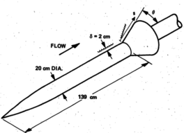
Figure 17. Solid body (from [18])

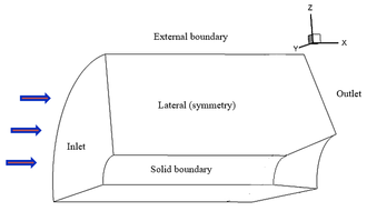
Figure 18. Domain and boundaries

Although this is an axisymmetric problem, its resolution is made here with a 3-D mesh, taking a quarter of the geometry by symmetry considerations. In addition, this problem was simulated by the dimensionless codes developed for this work. In the two lateral boundaries is imposed that the normal velocity component is zero. Inlet boundary conditions are:

;

The non-slip condition is applied on solid boundaries. Then

and

The temperature at the wall, which has a known value ${\textstyle (311\,K)}$ , is specified using the dimensionless specific internal energy:

and the outlet boundary conditions are specified using ${\textstyle {\boldsymbol {t}}_{j}}$ and ${\textstyle {\boldsymbol {q}}}$ .

The initial conditions are given by:

;

and

These initial values are defined in all nodes of the finite element mesh, except for the nodes where Dirichlet boundary conditions were prescribed.

Figure 19 shows the side view of the finite element mesh, which has 1 600 000 hexahedral elements. The mesh is the same as found in the NASA web repository for turbulence models (2-D with 2-zones of 81 $\times$ 101 and 81 $\times$ 101 nodes) but rotated to form a three-dimensional domain mesh corresponding to a quarter of the space surrounding the obstacle with 100 subdivisions in the quarter circumferential length. The total number of elements is $80\times (2\times 100)\times 100$ . Figure 20 shows a detailed view of the mesh where the flare starts.

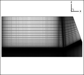
Figure 19. Finite element mesh

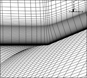
Figure 20. Mask in the zone where the cone begins

The mesh was refined near the wall such that the estimate of $y+$ is close to 0.5.

Using the safety factor ${\textstyle \beta =0.2}$ , the dimensionless time step is ${\textstyle \Delta t=}$ ${1.0}^{\ast }{10}^{-5}$ . The artificial viscosity coefficient used here is ${\textstyle {C}_{AD}=}$ $0.3$ .

Figure 21 compares the experimental velocity profiles with those obtained in this work and by the NASA WindUS program. The position in which these data were obtained corresponds to the plane ${\textstyle x=}$ $-6$ (the origin of coordinates ${\textstyle x}$ is located where the flare starts). Since there are no appreciable differences between the results obtained with TG, CBS and MTG, only the curve corresponding to the MTG scheme is shown here.

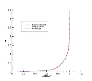
Figure 21. Comparison of velocity profiles

Figure 22 compares the temperature profiles for the same location. Both figures show proximity between the values obtained with the WindUS program [19] and the MTG code implemented in this work. In turn, results of both codes show a good agreement with the experimental data obtained in reference [18].

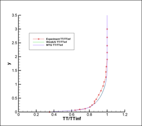
Figure 22. Comparison of temperature profiles

Figure 23 shows a comparison of the pressure distribution along the wall of the ogive. The ${\textstyle s}$ coordinate is measured along the surface of the solid with its origin ${\textstyle s=}$ $0\,$ located when the flare starts.

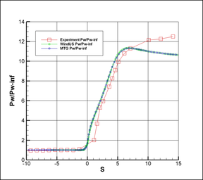
Figure 23. Pressure distribution on the wall

Finally, Figure 24 shows a comparison of the heat transfer through the wall of the solid obstacle. The definition of wall heat transfer ${\textstyle {q}_{w}}$ is given by: ${\textstyle {q}_{w}=}$ $-K\,{(dT/dy)}_{w}$ , where ${\textstyle K}$ is the thermal conductivity of the fluid (but here it is calculated from the corresponding dimensionless quantities).

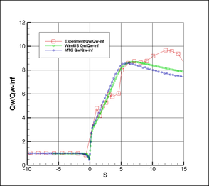
Figure 24. Heat transfer through the wall

A good agreement between results obtained with the MTG scheme and "WindUs" codes. As observed from Figure 23, the S-A model tends to slightly over-predict the pressure immediately downstream of the shock. Then the model starts to under-predict this quantity at ${\textstyle s=}$ $7$ approximately. The S-A model also under-predicts the heat transfer though the solid wall after position ${\textstyle s=}$ $7$ . The differences between the results of both codes and the experimental data for positions above ${\textstyle s=}$ $7\,$ can be attributed to the adopted RANS/FANS turbulence model (S-A), provided that all references show similar results [19,20].

Like the previous case, the convergence between the TG, MTG and CBS schemes does not differ significantly when the residuals are considered. However, there are differences in the relative wall clock computational times, as shown in Table 3.

Table 3. Relative computation times

Algorithm	Relative wall clock time
Single-step CBS	Not recommended
TG	1.0
TGM	1.03
CBS	1.30

It is observed that, for hypersonic flows, the three schemes (i.e. TG, MTG and CBS) are suitable from the point of view of convergence rates, but there are appreciable differences in terms of wall clock computational time, being the CBS scheme the most expensive.

The single-step CBS scheme was used for this case showing some numerical oscillations in the flare starting zone, showing again that this algorithm is not recommended for high Mach numbers.

8. Conclusions

Comparing density residuals, CBS and MTG methods show better convergence rate than the TG scheme. But the best convergence rate is obtained using CBS and MTG with local Δt_in. The TG method exhibits an oscillatory behavior in transonic and subsonic flows. This behavior is not observed when CBS or MTG schemes are used.

Using a local internal time step with the original TG method, density convergence is not improved, and pressure oscillation remains. However, by making a change in the stabilization term of the continuity equation with a blending function and using a local internal time step, the MTG scheme presents a convergence rate comparable to that obtained with the CBS method.

Although the CBS method does not require an iterative process, as required by the TG and MTG schemes, split operations are performed to calculate first an auxiliary momentum variable, which is used to obtain the density to finally update the momentum values. Then the energy and the S-A variable are calculated. These split operations imply in additional computational time cost. In addition, iterative terms of TG and MTG schemes converge rapidly with very few iterative steps and split operations are not necessary. These features make TG and MTG schemes more efficient than CBS method.

In this way, the MTG scheme is more efficient in terms of computational processing time than the CBS method and with a comparable convergence rate for all ranges of Mach numbers.

The alternative of the single-step CBS method, although efficient and suitable for transonic regimes, is not recommended for high Mach numbers, such as supersonic or hypersonic regimes.

With the modifications proposed here for the TG scheme, a modified method was obtained (the MTG scheme), which is the best option when convergence properties and computational processing times are considered for a wide range of Mach numbers.

References

[1] Donea J. A Taylor-Galerkin method for convective transport problems. International Journal for Numerical Methods in Engineering, 20:101-119, 1984.

[2] Yoon K.T., Moon S.Y., Garcia S.A., Heard G.W., Chung T.J. Flowfield-dependent mixed explicit-implicit (FDMEI) methods for high and low speed and compressible and incompressible flows. Computer Methods in Applied Mechanics and Engineering, 151:75-104, 1998.

[3] Burbridge H.P., Awruch A.M. A finite element Taylor-Galerkin scheme for 3-D numerical simulation of high compressible flow with analytical evaluation of element matrices. Hybrid Methods in Engineering, 2.I4:485-506, 2000.

[4] Burbridge H.P. O esquema explícito de Taylor-Galerkin na simulação numérica de escoamentos compressíveis tridimensionais utilizando elementos finitos hexaédricos de oito nós. Tese de mestrado. UFRGS, Porto Alegre, 1999.

[5] Zienkiewicz O.C., Taylor R.L. The finite element method. Vol. 3: Fluid Dynamics. Fifth edition, Butterworth Heinemann, Oxford, 2000.

[6] Zienkiewicz O.C., Codina R. A general algorithm for compressible and incompressible flow-Part I: The Split Charactestic-Based Scheme. International Journal for Numerical Methods in Fluids, 20:869-885, 1995.

[7] Boonmarlert P., Phongthanapanich S., Dechaumpai P. Combined characteristic-based split algorithm and Mesh Adaptation Technique for high-speed compressible flow analysis. Indian Journal of Engineering & Material Sciences, 12:376-388, 2005.

[8] Liu C.B., The Characteristic Based Split (CBS) scheme for laminar and turbulent incompressible flow simulations. Doctoral Thesis, University of Wales, Swansea, 2005.

[9] Massarotti N., Arpino F., Lewis R.W., Nithiarasu P. Explicit and semi-implicit CBS procedures for incompressible viscous flows. International Journal for Numerical Methods in Engineering, 66:1618-1640, 2006.

[10] Scungio M., Arpino F, Cortellessa G., Buonanno G. Detached eddy simulation of turbulent flow in isolated street canyons of different aspect ratios. Atmospheric Pollution Research, 6.I2:351-364, 2015.

[11] Zienkiewicz O.C., Satya Sai B.V.K., Morgan K., Codina R., Vázquez M. A general algorithm for compressible and incompressible flow-Part II: Tests on the Explicit Form. International Journal for Numerical Methods in Fluids, 20:887-913, 1995.

[12] Christon M.A. A domain-decomposition message-passing approach to transient viscous incompressible flow using explicit time integration. Computer Methods in Applied Mechanics and Engineering, 148:329-352, 1997.

[13] Allmaras S.R., Johnson F.T., Spalart P.R. Modifications and clarifications for the implementation of the Spalart-Allmaras turbulence model. Seventh International Conference on Computational Fluid Dynamics, ICCFD7-1902, 2012.

[14] White F. Viscous fluid flow. McGraw Hill Book Co, First edition, New York, 1974.

[15] Huebner K.H., Thornton E.A., Byrom T.G. The finite element method for engineers. Third Edition, John Wiley and Sons, Inc. New York, 1995.

[16] Nithiarasu P., Zienwkiewicz O.C. On stabilization of the CBS algorithm: Internal and external time steps, International Journal for Numerical Methods in Engineering, 48:875-880, 2000.

[17] Argyris J., Doltsinis I.S., Friz H. Hermes space shuttle: exploration of reentry aerodynamics. Computer Methods in Applied Mechanics and Engineering, 73:1-51, 1989.

[18] Kussoy M.I., Horstman C.C. Documentation of two- and three-dimensional hypersonic shock wave boundary layer interaction flows. NASA TM 101075, January 1989

[19] Georgiadis N.J., Rumsey Ch.L., Huang G.P. Revisiting turbulence model validation for high-mach number axisymmetric compression corner flows. 53rd AIAA Aerospace Sciences Meeting, AIAA 2015-0316, 2015.

[20] Erb A., Hosder S. Investigation of turbulence model uncertainty for supersonic/hypersonic shock wave-boundary layer interaction predictions. 22nd AIAA International Space Planes and Hypersonics Systems and Technologies Conference. September 2018.