Latest revision as of 12:50, 15 June 2018

Abstract

In this part of paper we shall extend the formulation proposed by Babuška and co-workers for robustness patch test, in quality assessment of error estimators, to more general cases of patch locations especially in three dimensional problems. This is performed first by finding an asymptotic finite element solution at interior parts of a problem with assumed smooth exact solution and then adding a correction part to obtain the solution near a kinked boundary irrespective of other boundary conditions at far ends of the domain. It has been shown that the solution corresponding to the correction part may be obtained in an spectral form by assuming a suitable proportionality relation between the nodal values of a mesh with repeatable pattern of macro-patches.

Having found the asymptotic finite element solution, the performance of error estimators may be examined. Although in this paper we focus on the asymptotic behavior of error estimators, the method described in this part may be used to obtain finite element solution for two/three dimensional unbounded heat/elasticity problems with homogeneous differential equations. Some numerical results are presented to show the validity and performance of the proposed method.

Keywords: Recovery, Error Estimate, Superconvergent, Robustness test, three dimensional, Unbounded domains

1. INTRODUCTION

Efforts by pioneering engineers in late twentieth century led to understanding the necessity of error evaluation and use of adaptive procedures in finite element solutions. Nowadays, most of commercial finite element programs are equipped with tools for error estimation and mesh generation. Nevertheless, the need for further investigation is still felt by scientists [1].

The knowledge of error estimation in two dimensional problems has now reached to a level of maturity [2]. However, advances in engineering and technology have led to increase of demands for three dimensional analyses and thus it is of great interest to know whether the error analyses still work well in three dimensions. Although many of the concepts introduced in two dimensional problems may readily be applied to three dimensions, there are many especial cases that may not comprehensively be covered by the counterparts studied in two dimensions. Quality assessment of error estimators may be considered as one of the cases.

There are two basic approaches employed in studies for assessment of error estimators. The most classic approach, used almost since the first thoughts of FEM, is benchmarking. This category of approach was employed in many early studies on error estimation, see [3,4] for example, and it is still being used as a tool for giving some evidences of good performance, e.g. [5,6]. Although benchmark problems in two and three dimensional spaces have much in common, dealing with the three dimensional ones may need some more elaboration. For example behavior of error estimators near an edge in 3D problem, where two intersecting boundary exist, may not easily be understood from the results obtained at edges of a 2D benchmark. In fact an edge in 3D problem has much in common with a corner in a 2D problem, yet not quite similar.

The second approach is employed for studies on quality of approximate error in asymptotic manner, i.e. when the element sizes tend to zero, and has roots in basic assumptions of finite element method. Although this type of assessment approach was inherently used by some researches to give proofs for theorems and lemmas regarding the convergence of the proposed methods, e.g. see [7], for the first time a systematic computer based type of the approach was introduced by Babuška et al in a series of papers [8-10]. Other researchers followed some similar approaches to explore superconvergence in plate problems [11, 12].

The method was basically introduced for assessment of error estimators applied at interior parts of a fictitious unbounded domain and has sound mathematical bases. The basic feature of the method is using meshes with repeatable patterns of patches in order to reduce the size of the space needed for the finite element solution. The test procedure is performed on a solution found for a single patch and thus, in this respect, resembles to the patch tests usually used in element technology. Since the reduction of the size of the domain, i.e. from an infinite size to a patch with finite size, is permitted under some assumptions for asymptotic behavior of the exact solution, the test results are interpreted in an asymptotic point of view. The formulation given for two dimensional problems is general and may be applied to three dimensional problems with no much effort.

The method was further extended to patch locations near boundaries in two dimensional problems [13]. The new formulation includes a boundary layer solution, in an asymptotic manner, for a fictitious unbounded domain. However, the modified version of the formulation can only be applied to a domain with single flat boundary. This means that the method may not be applied for patches near corners in two dimensional cases. Of course, this is of not much importance since the frequency of dealing with such situations is very small compared to other cases studied in two dimensional cases.

For three dimensional problems, however, the modified version can only be used for patch locations near a flat boundary. This means that the cases in which the patch is located near two intersecting flat boundaries, i.e. an edge, cannot be studied. It is obvious that frequency of such cases is not comparable with that of corners in two dimensional problems. However, if the problem is solved for edges of a three dimensional body, the formulation may also be applied for corners of a two dimensional problem.

In this paper we shall extend the formulation to the situations that the patch is near an edge/corner of the domain. We shall employ a spectral formulation in which a proportionality property plays a key role. It will be shown that the proportionality property has roots in the nature of the governing differential equation. As will be shown later in this paper, the governing equation for boundary layer solution in integral form is of a homogeneous type. The formulation given in this paper is not only useful for finding asymptotic boundary layer solution but also applicable to many other unbounded problems with governing equations of similar type. This is an important feature of the method. Having found the formulation for the boundary layer solution near kinked boundaries, the results will be verified by a sample problem with exact solution on an unbounded domain. The test results and the discussion for quality of the error estimates are given in the next part of the paper.

The layout of the paper is as follows; In Section 2 we shall prepare some preliminary formulations and definitions to be used in subsequent sections. In Section 3 some basic assumptions initially made in [8-10] and basic relations for the test at interior parts will be revisited. The relations will be frequently referred to especially when we describe the step by step test procedure in its generalized form. Having recalled the basic relations, the formulations used for flat boundaries, introduced in [13], will be given in brief followed by our proposed method which is to be applied for kinked boundaries. In Section 4 we shall present a sample problem to demonstrate that the proposed method is able to produce finite element solution for general unbounded domain with tractions or prescribed values at boundaries exhibiting decay condition. We shall conclude our discussions in Section 5.

2. PRELIMINARIES

In this section we prepare the preliminary tools for study of asymptotic behaviors of finite element solutions as well as error estimation schemes.

The problems of interest in this study are elliptic ones, e.g. heat transfer or elasticity problems, with generic differential equation/equations as

(1-a)

to be solved on ${\textstyle \Omega }$ with following boundary condition

on

(1-b)

and

on

(1-c)

Where ${\textstyle {\Gamma }_{u}\cap {\Gamma }_{t}=\varnothing }$ and ${\textstyle {\Gamma }_{u}\cup {\Gamma }_{t}=\partial \Omega }$ . In above ${\textstyle {\boldsymbol {S}}}$ is a suitable operator for defining the gradients of ${\textstyle {\boldsymbol {u}}}$ , ${\textstyle {\boldsymbol {D}}}$ is a suitable matrix for modulus of material and ${\textstyle {\boldsymbol {t}}}$ is a traction vector associated with the problem type. Also ${\textstyle {\boldsymbol {\tilde {n}}}}$ is a matrix containing components of unit normal to the boundary arranged in an appropriate form for heat or elasticity problems.

Discretization of the domain to a series of elements and approximation of ${\textstyle {\boldsymbol {u}}}$ as ${\textstyle {\boldsymbol {u}}\cong {\boldsymbol {u}}_{h}={\boldsymbol {N}}{\boldsymbol {\overline {u}}}_{h}}$ and application of Galerkin type of weighted residual formulation in weak form (or equivalent minimization of a suitable functional) leads to following well known matrix equation

(2)

Where ${\textstyle {\boldsymbol {N}}}$ is the set of shape functions used and also ${\textstyle {\boldsymbol {B}}\equiv {\boldsymbol {SN}}}$ . It is noteworthy to remember that the following relation always exists between the exact solution and the finite element one

(3)

Generally there will be a discrepancy between the exact solution, which is not available for most problems, and the finite element solution. This deviation constitutes the error at each point

(4-a)

The error distribution can also be expressed in terms of the gradients

or

(4-b)

Where ${\textstyle {\sigma }_{ex}={\boldsymbol {D}}{\epsilon }_{ex}={\boldsymbol {DS}}{\boldsymbol {u}}_{ex}}$ and ${\textstyle {\sigma }_{h}={\boldsymbol {D}}{\epsilon }_{h}={\boldsymbol {DB}}{\boldsymbol {\overline {u}}}_{h}}$ .

If the shape functions are chosen properly, reduction of the maximum mesh size must result to reduction of errors, i.e. ${\textstyle {\boldsymbol {e}}\rightarrow {\boldsymbol {0}}}$ as ${\textstyle h_{max}\rightarrow 0}$ . This is usually referred to as completeness of the set of shape functions.

It is a priori understood that in absence of any singularity in the domain, the ideal rate for convergence of the finite element errors is of order ${\textstyle O(h^{P+1})}$ for ${\textstyle {\boldsymbol {e}}_{u}}$ and ${\textstyle O(h^{P})}$ for ${\textstyle {\boldsymbol {e}}_{\epsilon }}$ and ${\textstyle {\boldsymbol {e}}_{\sigma }}$ where ${\textstyle h}$ is an average mesh size for the solution. This simple information constitutes a basis for study of error behavior and evaluation of error estimates in asymptotic form.

2.1 Error estimation

Approximate evaluation of error can be performed through estimation of its absolute value, irrespective of the signs, or calculation of the difference between a set of enhanced answers and those of finite element method. Most of residual based error estimators fall within the former approach and almost all recovery based error estimators employ the latter approach.

In an error analysis a suitable norm is usually defined to give an indication for the exact error level over the whole domain, e.g. ${\textstyle L_{2}}$ norm of errors

or

(5)

Here ${\textstyle {\Omega }^{'}}$ represents a partition of the domain where the error analysis is to be performed. When evaluation of an error estimator is required, benchmark problems with exact solution are selected and the true error and the approximate one are compared. Having evaluated approximate errors, i.e. ${\textstyle {\boldsymbol {e}}_{u}^{\ast }}$ , ${\textstyle {\boldsymbol {e}}_{\epsilon }^{\ast }}$ or ${\textstyle {\boldsymbol {e}}_{\sigma }^{\ast }}$ , a dimensionless parameter as the ratio of the error values, called “effectivity index”, is defined to show the quality of error estimates

(6)

where

(7)

Obviously when ${\textstyle \theta }$ is close to unity, the performance of the estimator is considered satisfactory. It is expected that the effectivity index tend to unity when the mesh size is reduced sufficiently, i.e. ${\textstyle \theta \rightarrow 1}$ as ${\textstyle h\rightarrow 0}$ . If such a property exists, the error estimator is called “asymptotically exact” [14]. It has been shown that only few estimators exhibit such a property (the reader may consult to references 3,4 and 10).

However, in study of asymptotic behavior of error estimators, it happens that the asymptotic effectivity indices take values close to unity. When comparison of different types of estimators is aimed, an error estimator is said to be more robust if the effectivity index calculated is closer to unity.

3. ROBUSTNESS PATCH TEST

In this section we describe the test introduced by Babuška et al in 1994. Although the procedure can be found, with many proofs for theorems and lemmas, in references [8] and [9] we repeat the core of the formulation here since it is needed for generalization of the formulation to wider set of cases.

The test is basically a patch test since all computations at last is performed on a small group of elements with specific boundary conditions. The whole procedure resembles to the patch tests usually employed for examining completeness of shape functions in element technology. The reader can find the basis and history of such patch tests in reference [15]. But before explaining the robustness test, it is worthy to recall the basic features of the patch test in element technology in order to comprehend similarities and differences with the robustness patch test for error estimators.

It is well understood that if in a simple patch test an element can reproduce an exact field with order similar to the order of the shape functions then the asymptotic rate of convergence of the solution is guaranteed. The test is in fact a finite element solution on a group of elements with boundary conditions extracted from the exact field. The choice of boundary condition for such a test is trivial to determine and this is usually accomplished by considering prescribed values for main function, i.e. displacements, or its derivatives as prescribed tractions.

It may be thought that similar strategy is applicable when asymptotic convergence of an error estimate, e.g. a superconvergent one, is to be studied. It is true in some respects but the test will not be a complete one. It is possible to construct a test on a group of elements with prescribed boundary conditions extracted from a polynomial, as an exact solution, with one order higher than that of the shape functions. In such a study the aim will be evaluation of capability of reproducing the exact errors. But we note that the boundary conditions considered are not necessarily similar to those which exist between the patches of elements in a real finite element solution. Therefore the results obtained from such a patch test may be considered just as a rough indication for capability of the error estimator.

The deficiency is removed in the patch test proposed by Babuška et al in an elegant manner. The test is constructed by some basic assumptions for mesh configuration and smoothness of the solution. The robustness of an error estimation, in a norm as (5) for instance, is defined by evaluation of upper and lower bounds, ${\textstyle {\theta }_{L}}$ and ${\textstyle {\theta }_{U}}$ , for effectivity index of (6). Therefore the following index is defined

(8)

If the error estimator precisely reproduces the error then ${\textstyle {\theta }_{L}={\theta }_{U}=1}$ and thus ${\textstyle R=0}$ . However for practical use, robustness values between ${\textstyle 0.8<R<1.2}$ are considered ideal. Since the assessment is performed in an asymptotic manner, the exact solution for evaluation of the exact error is considered as a polynomial of one order higher than that of shape functions representing largest terms in a Taylor expansion of error when the size of elements, at limit, is infinitesimal.

3.1 Assumptions

The fundamental assumptions are as follows

It is assumed that in all directions the mesh is locally uniform and is composed of a series of repeatable pasterns, as the basic cell with dimension ${\textstyle h}$ especially inside ${\textstyle {\Omega }_{1}}$ in Figure 1. A single cell of the repeatable pattern is considered as a patch for the test. The reader may notice that such patches have different definitions from the ones used for recovery methods. Note that no assumption is made about the mesh outside of ${\textstyle {\Omega }_{1}}$ .


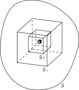
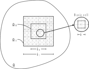
(a)	(b)

Figure 1. The domain, subdomain and basic cell considered for robustness patch test; (a) Three dimensional presentation of the domain; (b) Projection of the domain on a two dimensional plane.

Study on asymptotic convergence of the solution requires that the elements sizes be close to zero and so the dimensions of patches consisting a number of such elements like patches shown in Figure 1, i.e. basic cell with dimension ${\textstyle h}$ and the larger patches with dimensions ${\textstyle h_{0}}$ and ${\textstyle h_{1}}$ ( ${\textstyle h_{0}}$ and ${\textstyle h_{1}}$ are multiples of ${\textstyle h}$ ). In this regard it is also assumed that that ${\textstyle h}$ tends to zero with a faster rate than ${\textstyle h_{0}}$ (and ${\textstyle h_{1}}$ ). Moreover, it is assumed that the basic cells are cuboid (in three dimensions) with edges parallel to axes, though this is not necessary in general.

It is assumed that the exact solution is smooth at vicinity of the patch, i.e. inside macro patch ${\textstyle {\Omega }_{1}}$ . This means that the exact solution has bounded ${\textstyle \left(p+2\right)}$ derivatives at the location of the patch (or in other words the patch is far from singular points). Besides, not all of the derivatives with order of ${\textstyle \left(p+1\right)}$ vanish at the location of the patch.

The mesh is sufficiently refined outside ${\textstyle {\Omega }_{1}}$ such that the error converges almost with the optimal rate in ${\textstyle L_{2}}$ norm in ${\textstyle {\Omega }_{1}}$ , i.e.:

${\textstyle {\Vert {\boldsymbol {e}}_{u}\Vert }_{L_{2},{\Omega }_{1}}\leq Ch^{p+1-\lambda }}$

where ${\textstyle C}$ is a constant independent of ${\textstyle h}$ , and ${\textstyle \lambda }$ representing the power of singularity, is sufficiently small. This means that the pollution error is negligible. This assumption practically holds for meshes created by adaptive algorithms which try to distribute, equally, the energy norm of the error over the elements.

3.2 Basic features of the test

Before focusing on the error, asymptotic finite element solutions should be obtained. This means that the problem of (1) should be solved either irrespective of the main boundary conditions, when the patch is located inside, or just with condition specified when the patch located close to a boundary but still irrespective of other boundary conditions. The information available is that the exact solution, in asymptotic sense, is of a polynomial form. If such a finite element solution is obtained the results are generalized to many problems with similar type and different conditions at boundaries. Error evaluation comes after determining the finite element solution.

From the smoothness assumptions it is concluded that the exact solution may be written in the form of a Taylor series around a point inside the macro-patch ${\textstyle {\Omega }_{0}}$ as

(9)

with ${\textstyle a_{i}}$ being appropriate coefficients and ${\textstyle \Delta x=x-x_{0}}$ and so forth for ${\textstyle \Delta y}$ and ${\textstyle \Delta z}$ where ${\textstyle x_{0}}$ , ${\textstyle y_{0}}$ and ${\textstyle z_{0}}$ are coordinates of a point inside the patch. With the knowledge of asymptotic convergence of the finite element solution it follows that it is just necessary to consider a complete polynomial of order ${\textstyle \left(p+1\right)}$ as the asymptotic exact solution. For scalar problems, for instance

,

.

(10)

Here ${\textstyle X}$ , ${\textstyle Y}$ and ${\textstyle Z}$ are suitable normalized coordinates. For testing the estimates on linear elements in three dimensional elasticity problems, for example, we write the polynomial vector as

,

(11)

where ${\textstyle {\boldsymbol {1}}_{1}={\langle {\begin{array}{ccc}1&0&0\end{array}}\rangle }^{T}}$ , ${\textstyle {\boldsymbol {1}}_{2}={\langle {\begin{array}{ccc}0&1&0\end{array}}\rangle }^{T}}$ and ${\textstyle {\boldsymbol {1}}_{3}={\langle {\begin{array}{ccc}0&0&1\end{array}}\rangle }^{T}}$ .

Now with the aid of the following trivial relation

(12)

in which ${\textstyle {\boldsymbol {\overline {u}}}_{ex}}$ is a vector of exact values at nodal points of the mesh, one may use Equation (3) and write

(13)

Wherever the mesh is repeated, the right hand side of (13) is a periodic function since ${\textstyle {\boldsymbol {u}}_{ex}-{\boldsymbol {N}}{\boldsymbol {\overline {u}}}_{ex}}$ is periodic. The proof is very easy and can be accomplished by writing the monomials of (10) or (11) locally in each element and substituting in expression of ${\textstyle {\boldsymbol {u}}_{ex}-{\boldsymbol {N}}{\boldsymbol {\overline {u}}}_{ex}}$ . It follows that the new function is not dependent on the position of the origin of the local coordinates and therefore if the element pattern is repeated the function will be repeated as well (see [16] for more explanations).

The repeatability property of the right hand side of Equation (13) plays a key role in reducing the size of the problem to be solved. The periodic nature of the right hand side of (13) leads to repeatability of the left hand side of the equation. Therefore one may write the equation on a smallest repeatable unit of the mesh, or on a larger repeatable portion consisting of the units, here known as ${\textstyle {\Omega }^{'}}$

(14)

in which ${\boldsymbol {\overline {u}}}_{h}^{p}={\boldsymbol {\overline {u}}}_{h}-$ ${\boldsymbol {\overline {u}}}_{ex}$ . Equation (14) should of course be solved with a set of periodic boundary conditions. In the next subsection we shall see that depending on the patch location ${\textstyle {\Omega }^{'}}$ may be interpreted as a patch volume itself or volume of a column of patches normal to the boundary.

It can be seen that Equation (14) is insensitive to constant values for ${\textstyle {\boldsymbol {\overline {u}}}_{h}^{p}}$ , i.e. rigid body motion of the solution. This implies that after finding ${\textstyle {\boldsymbol {\overline {u}}}_{h}^{p}}$ , as will be described later, the asymptotic finite element solution is obtained as

(15)

Where ${\textstyle {\boldsymbol {C}}}$ is a vector containing constant values and is evaluated from equivalence of mean values for the exact and finite element solutions [9, 10, 13, 16]

(16)

Having found the asymptotic finite element solution from ${\textstyle {\boldsymbol {u}}_{h}={\boldsymbol {N}}{\boldsymbol {\overline {u}}}_{h}}$ , the exact norm of errors and that of estimated ones are calculated. Since the exact solution is expressed in terms of monomials with unknown coefficients ${\textstyle {\boldsymbol {a}}}$ , as Equation (10) or (11), the norms of errors in squared form can be written as

(17)

With analogy, the approximate error may also be written as

(18)

This makes it easy to find the upper and lower bounds of the squared effectivity index

(19)

by evaluation of eigenvalues of the following matrix

(20)

Where the matrix ${\textstyle {\boldsymbol {H}}}$ is defined as

,

(21)

In above equation ${\textstyle \Psi }$ and ${\textstyle \Lambda }$ are normalized eigenvectors and diagonal matrix of eigenvalues of ${\textstyle {\boldsymbol {E}}_{0}}$ , respectively. Hence

,

(22)

It should be noted that relations (12) to (16) are useful for reducing the size of the problem only when a sort of periodicity exists in the solution. This will be the case as long as the exact solution is expressed in terms of monomials of order ${\textstyle p+1}$ and the mesh pattern is repeatable. When the patch is far enough from the main boundary conditions, i.e. located at interior of the domain, the periodicity may be assumed for all directions. This allows us to reduce the size of the problem to a domain as small as a patch. In the case that patch is located near a boundary, the repeatability of the mesh is lost in normal direction to the boundary and thus the solution loses its periodicity in that direction. This latter case needs additional treatment which we shall briefly explain in the forthcoming subsections. In the case that the patch is located at a corner of the main domain, the periodicity will be lost in all directions. We shall also refer to this case after revisiting the patch test near a single flat boundary.

3.3 Patch test at interior parts of the domain

As mentioned above, when patch is located at interior parts of the domain, the patch pattern is considered repeatable in all directions. Now since the source term in the right hand side of (14) is repeatable, the finite element solution will be periodic. This allows us to write Equation (14) just on a single patch as

(23)

which is to be solved with periodic boundary conditions i.e.

${\boldsymbol {\overline {u}}}_{h(Z+L_{z})}^{p}={\boldsymbol {\overline {u}}}_{h(Z)}^{p}$

(24)

with ${\textstyle L_{x}}$ , ${\textstyle L_{y}}$ and ${\textstyle L_{z}}$ being the patch dimensions (period length) along the three directions. Having found the periodic solutions, the asymptotic finite element solution is evaluated from (15) and (16). The test procedure will be completed by estimating the errors and calculation of upper and lower bounds of the effectivity index as indicated in Equations (17) to (22).

3.4 Patch test at parts near flat boundaries

To extend the formulation to more general cases, here we revisit the procedure near flat boundaries. Now supposing that a flat boundary exists at ${\textstyle z=0}$ and the patch pattern is repeatable in all directions. Equation (14) may be rewritten as

(25)

Clearly the periodicity of solution is lost along z axis since the repeatability of the patch pattern is terminated at ${\textstyle z=0}$ although the source term is still periodic. Hence an additional solution is considered, as boundary layer type, to those obtained for interior parts

(26)

Substituting (26) in (25) and noting that (14) holds for solutions pertaining to interior patches, then provided that no extra forces is imposed from boundaries, i.e. when dealing with Dirichlet boundary conditions, the following integral equation is obtained

(27)

It is clear that as we go far from the boundary, i.e. ${\textstyle z\rightarrow \infty }$ , we should obtain ${\textstyle {\boldsymbol {\overline {u}}}_{hB}^{p}\rightarrow {\boldsymbol {\overline {u}}}_{h}^{p}+}$ ${\boldsymbol {C}}$ . Therefore Equation (27) must be solved with two periodic conditions along ${\textstyle x}$ and ${\textstyle y}$ and following decay condition

(or

) when

(28)

Where ${\textstyle d_{z}}$ denotes the distance along ${\textstyle z}$ . It may be noted that decay condition on ${\textstyle {\boldsymbol {\overline {u}}}_{h0}^{p}}$ is stronger than the one defined for its gradients, i.e. ${\textstyle {\boldsymbol {B}}{\boldsymbol {\overline {u}}}_{h0}^{p}}$ . In fact application of decay condition in latter form may lead to constant values of ${\textstyle {\boldsymbol {\overline {u}}}_{h0}^{p}}$ for large values of ${\textstyle z}$ which is still consistent with formulation for interior parts since constant values are considered a priori. This is true basically when we are dealing with asymptotic finite element solutions in which the solutions for two fictitious domains are added together as Equation (26). However, when a general unbounded domain is to be solved, constant values for the solution at far ends of the domain may have no physical meaning and thus in such situations the first form of decay condition must be satisfied rigorously. In a sample problem we shall give solution to an unbounded domain in order to verify the method to be described in sequel.

The boundary conditions considered in this study are

1. Dirichlet boundary condition: In this type we apply

(29)

Substitution of (26) instead of the last two terms in right hand of (15) as

(30)

and application of (29) leads to following condition

(31)

From which it follows that

(32)

If homogeneous Dirichlet condition is of concern then the monomials in (10) or (11) should be

chosen accordingly.

2. Neumann boundary condition: In this type of condition the tractions extracted from the exact solution are applied to the boundary of the domain, i.e.

(33)

to be substituted in (1-c). If Equation (2) is rewritten with ${\textstyle {\boldsymbol {\overline {u}}}_{h}}$ replaced with its equivalent from (26) and (27) then

(34)

Where

(35)

It follows that

(36)

In fact we only need to consider elements near boundary since Equation (27) holds for interior parts. Therefore

(37)

In above ${\textstyle {{\Omega }^{'}}_{bnd}}$ denotes volume of all elements in the column having at least one node on the boundary, ${\textstyle {\left({\boldsymbol {\overline {u}}}_{h0}^{p}\right)}_{bnd}}$ denotes associative subset of ${\textstyle {\boldsymbol {\overline {u}}}_{h0}^{p}}$ , and ${\textstyle {\boldsymbol {F}}_{prs}}$ represents the right hand side of Equation (36).

Now we are ready to apply the boundary condition to a problem asymptotically modeled with a periodic mesh pattern and a single flat boundary. Considering a 3D mesh of patches like Figure 2-a, we assume that the boundary exists at plane ${\textstyle z=0}$ . The mesh pattern is considered repeatable along ${\textstyle x}$ , ${\textstyle y}$ and ${\textstyle z}$ , with ${\textstyle -\infty <x<\infty }$ , ${\textstyle -\infty <y<\infty }$ and ${\textstyle 0<z<\infty }$ . A column of patches along ${\textstyle z}$ is selected. For simplicity we use Figure 2-b instead of Figure 2-a as a two dimensional presentation of the three dimensional column. Note that we are aiming at solving Equation (27) or (37) in which ${\textstyle {\Omega }^{'}}$ is volume of the column.


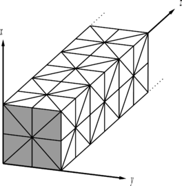
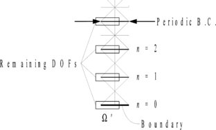
(a)	(b)

Figure 2. A column with infinite length; (a) Three dimensional presentation of the column with one end at boundary consisting of repeatable patterns as basic cells, (b) Two dimensional presentation of the infinite column with repeatable pattern and the numbering used for different levels.

After numbering the patch levels consecutively towards the middle of the domain as shown in Figure 2-b, in the matrix equation of each patch the degrees of freedoms not falling on interfaces of patches are statically condensed. The matrix equation of the asymptotic finite element solution pertaining to the remaining degrees of freedoms is assembled as

{\left[{\begin{array}{ccccccccc}{\boldsymbol {k}}_{0,0}&{\boldsymbol {k}}_{0,1}&&&&&&&\\{\boldsymbol {k}}_{1,0}&{\boldsymbol {k}}_{1,1}&{\boldsymbol {k}}_{1,2}&&&&&&\\&{\boldsymbol {k}}_{2,1}&{\boldsymbol {k}}_{2,2}&{\boldsymbol {k}}_{2,3}&&&&&\\&&&&\ddots &&&&\\&&&&&{\boldsymbol {k}}_{n,n-1}&{\boldsymbol {k}}_{n,n}&{\boldsymbol {k}}_{n,n+1}&\\&&&&&&&&\ddots \end{array}}\right]}_{\infty \times \infty }\cdot {\left\{{\begin{array}{c}{\boldsymbol {\overline {u}}}_{h0}^{p,0}\\{\boldsymbol {\overline {u}}}_{h0}^{p,1}\\{\boldsymbol {\overline {u}}}_{h0}^{p,2}\\\vdots \\{\boldsymbol {\overline {u}}}_{h0}^{p,n-1}\\{\boldsymbol {\overline {u}}}_{h0}^{p,n}\\{\boldsymbol {\overline {u}}}_{h0}^{p,n+1}\\\vdots \end{array}}\right\}}_{\infty \times 1}={\left\{{\begin{array}{c}{\boldsymbol {F}}_{0}\\{\boldsymbol {0}}\\{\boldsymbol {0}}\\\vdots \\{\boldsymbol {0}}\\{\boldsymbol {0}}\\{\boldsymbol {0}}\\\vdots \end{array}}\right\}}_{\infty \times 1}

(38)

Where ${\textstyle {\boldsymbol {k}}_{m,n}={\boldsymbol {k}}_{n,m}^{T}}$ is the relative stiffness matrix of ${\textstyle m}$ th and ${\textstyle n}$ th levels, and ${\boldsymbol {\overline {u}}}_{h0}^{p,k}$ is the set of nodal values at level ${\textstyle k}$ .

It can be seen that each row of the matrix represents the relation between levels ${\textstyle n-1}$ , ${\textstyle n}$ and ${\textstyle n+1}$ except for the first level. Also, since the patch pattern is the same for all levels, the out of diagonal matrices, below and above the diagonal, are similar. Extracting the ${\textstyle n}$ th row of the matrix Equation (38), one can show it as

(39)

By appropriate arrangement we have

\left[{\begin{array}{cc}{\boldsymbol {A}}&{\boldsymbol {B}}\\{\boldsymbol {0}}&{\boldsymbol {I}}\end{array}}\right]\cdot \left\{{\begin{array}{c}{\boldsymbol {\overline {u}}}_{h0}^{p,n+1}\\{\boldsymbol {\overline {u}}}_{h0}^{p,n}\end{array}}\right\}=\left[{\begin{array}{cc}{\boldsymbol {0}}&-{\boldsymbol {C}}\\{\boldsymbol {I}}&{\boldsymbol {0}}\end{array}}\right]\cdot \left\{{\begin{array}{c}{\boldsymbol {\overline {u}}}_{h0}^{p,n}\\{\boldsymbol {\overline {u}}}_{h0}^{p,n-1}\end{array}}\right\}

(40)

Supposing that the coefficient matrix in the left hand side of (40) is invertible, it follows that

\left\{{\begin{array}{c}{\boldsymbol {\overline {u}}}_{h0}^{p,n+1}\\{\boldsymbol {\overline {u}}}_{h0}^{p,n}\end{array}}\right\}=\left[{\begin{array}{cc}-{\boldsymbol {A}}^{-1}{\boldsymbol {B}}&-{\boldsymbol {A}}^{-1}{\boldsymbol {C}}\\{\boldsymbol {I}}&{\boldsymbol {0}}\end{array}}\right]\cdot \left\{{\begin{array}{c}{\boldsymbol {\overline {u}}}_{h0}^{p,n}\\{\boldsymbol {\overline {u}}}_{h0}^{p,n-1}\end{array}}\right\}

(41)

One may write a relation between two sets of such defined vectors for two levels, say levels ${\textstyle m}$ and ${\textstyle n}$ , as

\left\{{\begin{array}{c}{\boldsymbol {\overline {u}}}_{h0}^{p,n+1}\\{\boldsymbol {\overline {u}}}_{h0}^{p,n}\end{array}}\right\}={\left[{\begin{array}{cc}-{\boldsymbol {A}}^{-1}{\boldsymbol {B}}&-{\boldsymbol {A}}^{-1}{\boldsymbol {C}}\\{\boldsymbol {I}}&{\boldsymbol {0}}\end{array}}\right]}^{n-m}\cdot \left\{{\begin{array}{c}{\boldsymbol {\overline {u}}}_{h0}^{p,m}\\{\boldsymbol {\overline {u}}}_{h0}^{p,m-1}\end{array}}\right\}

(42)

Solution of above recursive relation can be obtained by transformation of the variables to a space with bases of normalized eigenvectors of the coefficient matrix in Equation (41). Invariably, the eigenvalue problem may be solved using matrices in Equation (40), as a generalized eigenvalue problem, to avoid problems encountering for inversion of ${\textstyle {\boldsymbol {A}}}$ . Therefore following generalized eigenequation is defined

or

(43)

Solution of the eigenequation of (43) results in a series of eigenvalues ${\textstyle {\mu }_{i}}$ and eigenvectors ${\textstyle {\boldsymbol {w}}_{i}}$ , as many as two times of DOFs at each level, from which those with decay property, as ${\textstyle \vert {\mu }_{i}\vert \leq 1}$ , are nominated for construction of the asymptotic finite element solution. We note that in the new space constructed by series of ${\textstyle {\boldsymbol {w}}_{i}}$ the recursive relation for each base vector at two different levels, ${\textstyle m}$ and ${\textstyle n}$ , is written as

(44)

Also each eigenvector is of the form

(45)

Now assume that the column with infinite length is cut and the boundary conditions are to be imposed at current level with nodal values as ${\textstyle {\varphi }_{i}}$ . If the levels are renumbered accordingly then for ${\textstyle n}$ levels farther the correction to the periodic finite element solution is evaluated as

(46)

In which ${\textstyle n_{c}}$ is the number of DOFs at each level and ${\textstyle c_{i}}$ denotes the unknown coefficient for the mode number ${\textstyle i}$ to be determined from the boundary condition specified in (31) or (37).

Having found the correction required for boundaries, ${\textstyle {\boldsymbol {\overline {u}}}_{h0}^{p}}$ , the periodic finite element solution may be calculated as Equation (26). Finally, the asymptotic finite element solution is obtained as

(47)

Now one can apply the error estimation procedure to study its asymptotic convergence behavior.

As is seen the formulation is suitable for flat boundaries only. In case that the patch is located near a kinked boundary the periodicity of the solution is lost along to directions normal to the edge line. The problem becomes worse when a corner patch near intersection of three planes, is considered. In this latter case the periodicity is lost along all directions. In the next section we shall extend the formulation to such wider range of applications.

3.5 Generalization of the test for application to patches near kinked boundaries

In this section we shall give a more general formulation for evaluation of the asymptotic finite element solutions near edges or corners of a three dimensional domain.

We assume that two intersecting planes exist at ${\textstyle x=0}$ and ${\textstyle y=0}$ making a straight edge along ${\textstyle z}$ axis (Figure 3). A repeatable mesh pattern is again constructed. Since the problem is studied in asymptotic form, the mesh is considered to be consisting of infinite number of patches along the three axes. Equation (25) is again written

(48)


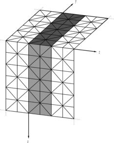
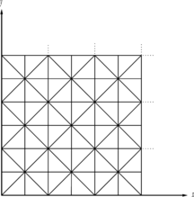
(a)	(b)

Figure 3. A typical case for patch location near two intersecting flat boundaries; (a) The domain shaded in gray is an unbounded domain along ${\textstyle x}$ and ${\textstyle y}$ axes and is of a single-cell-width thickness, (b) Two dimensional presentation of patch location near kinked boundaries which is similar to a corner point.

Here ${\textstyle {\Omega }^{'}}$ represents an infinite domain with thickness of a patch along ${\textstyle z}$ axes since the periodicity of the solution retains just along ${\textstyle z}$ . To avoid confronting difficulties for three dimensional presentation of the problem, we look in to the problem as a two dimensional one, i.e. its projection on ${\textstyle x}$ ${\textstyle y}$ plane (see Figure 3-b). Again we assume that the asymptotic periodic solution is consisting of two parts as Equation (26) substitution of which in (48) gives similar equation as (27). Clearly the solution must be found satisfying Dirichlet or Neumann boundary conditions similar to (30) or (37) and two decay conditions along ${\textstyle x}$ and ${\textstyle y}$ . Thus the statement of the problem is to solve

(49)

with boundary conditions (also see (32) and (37))

or

(50)

at ${\textstyle x=0}$ or ${\textstyle y=0}$ , periodic conditions along ${\textstyle z}$ and following decay conditions

(or

) when

and

(51)

Where here again ${\textstyle d_{x}}$ and ${\textstyle d_{y}}$ denote distances along ${\textstyle x}$ and ${\textstyle y}$ .

The key point of the solution is isolation of a patch from , as before, and writing suitable relations between the DOFs. Supposing that the solution may be found spectrally in an appropriate space, some proportionality relations are assumed between adjacent patches. The reason for assuming such relations may be explored in Appendix. For instance in Figure 4-a following relations are considered

,

(52-a)

for direction and

,

(52-b)

for ${\textstyle y}$ direction. Similar relation is valid for any two nodes with distance ${\textstyle L_{x}}$ or ${\textstyle L_{y}}$ for example

,

(52-c)

and so forth. In above ${\textstyle {\boldsymbol {\overline {u}}}}$ denotes spectral nodal values in a new space to be defined later.


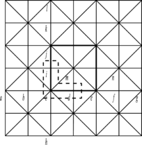
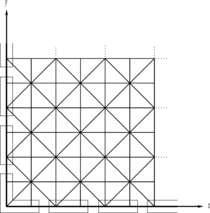
(a)	(b)

Figure 4. A macro patch consisting of ${\textstyle 3\times 3}$ patches; (a) The proportionality relations are written as (52), between nodal values along both directions, (b) Schematic presentation of nodes in the macro patch nominated for satisfaction of the boundary condition.

Now the solution starts with writing all relations similar to (52) for a patch and all surrounding ones, i.e. nine patches in Figure 4, in a matrix form. It can be seen that all nodal values may be written in terms of few of them in central patch. Note that the nodal values inside the central patch must be condensed before writing the proportionality relations. Thus the remaining nodal values will be those located at two edges of patches, i.e. left and bottom edges. Hence if we focus on all similar DOFs at the two similar sides of the patches, the following matrix relation containing proportionality properties, like relations (52), can be written

(53)

Where ${\textstyle {\boldsymbol {\overline {u}}}_{D}}$ and ${\textstyle {\boldsymbol {\overline {u}}}_{I}}$ denote dependent and independent nodal values in macro patch of ${\textstyle 3\times 3}$ in Figure 4-a. The independent nodal values in Figure 4-a may be considered as those falling in the dash line area. The reader may notice that the relation may also be written in a macro patch. Here again the matrix equation obtained from (49) may be presented as (38). To avoid difficulties pertaining to numbering of the patches along two or three axes, we use an abstract notation with rearranged form as the following one

\left[{\begin{array}{cc}{\boldsymbol {K}}_{II}&{\boldsymbol {K}}_{ID}\\{\boldsymbol {K}}_{DI}&{\boldsymbol {K}}_{DD}\end{array}}\right]\cdot \left\{{\begin{array}{c}{\boldsymbol {\overline {u}}}_{I}\\{\boldsymbol {\overline {u}}}_{D}\end{array}}\right\}=\left\{{\begin{matrix}{\boldsymbol {0}}\\{\boldsymbol {f}}\end{matrix}}\right\}

(54)

The first row of the above matrix equation represents a generic row of a matrix equation similar to (38) and the second row represents the remaining of the equations most of which have zero right hand side, i.e. components of ${\textstyle {\boldsymbol {f}}}$ , except for the ones corresponding to nodes at Neumann boundaries. Substituting (53) in (54), the first set of equations gives

(55)

In which

(56)

Equation (55) means that ${\textstyle {\boldsymbol {\overline {u}}}_{I}}$ may be constructed from vectors in null space of ${\textstyle {\boldsymbol {Q^{'}}}}$ . To evaluate such null space the determinant of ${\textstyle {\boldsymbol {Q}}^{'}}$ is set to be zero

(57)

It may be observed that two unknowns, ${\textstyle {\mu }_{1}}$ and ${\textstyle {\mu }_{2}}$ , appear in one equation. This means that numerous pairs may be found satisfying Equation (57). To solve the problem one may choose a value for one unknown and find the other through the characteristic equation. Hence

(58)

To satisfy the decay condition (51) we define another function as

(59)

Generally, several relations like (59) exist since characteristic equation (57) possesses several roots for a given ${\textstyle {\mu }_{1}}$ . Therefore

when

,

(60)

Now supposing that ${\textstyle {\phi }_{{\mbox{ }}i{\mbox{ }}{\mbox{ }}({\mu }_{1})}}$ belongs to the null space of ${\textstyle {\boldsymbol {Q^{'}}}}$ , one may write the non trivial solution of (55) as

(61)

Where integration is taken over all feasible values of ${\textstyle {\mu }_{1}}$ . In Equation (61) coefficients ${\textstyle c_{i({\mu }_{1})}}$ are to be determined from boundary conditions at ${\textstyle x=0}$ or ${\textstyle y=0}$ . The number of inner summation is dependent on the number of ${\textstyle {\phi }_{{\mbox{ }}i{\mbox{ }}{\mbox{ }}({\mu }_{1})}}$ for which ${\textstyle {\mu }_{1}}$ and ${\textstyle {\mu }_{2}}$ satisfy (59) and may vary when ${\textstyle {\mu }_{1}}$ falls within different regions.

Since ${\textstyle {\mu }_{1}}$ may take complex values the symbolic integral of (61) is taken over a feasible area on Gaussian plane. Because the decay condition imposes the condition of ${\textstyle \vert {\mu }_{1}\vert \leq 1}$ , the feasible area is a circle with radios of unity and center at origin. However, we note that for problems with real differential equation, the exact solution and the finite element one should be real. This means that from values in feasible domain those leading to real answers should be selected implying that the complex values, and the associated vectors, should be in the form of conjugate pairs. Thus the integration in (61) should in fact be taken over real values for ${\textstyle {\mu }_{1}}$ while letting ${\textstyle {\mu }_{2}}$ to be complex. To ensure that all real values are covered by ${\textstyle {\mu }_{1}}$ and ${\textstyle {\mu }_{2}}$ Equation (61) may be rewritten as

(62)

or

(63)

where of course it is needed to find ${\textstyle {\mu }_{1}}$ in terms of ${\textstyle {\mu }_{2}}$ as Equation (58) and (59). Note that the negative values have been excluded from the integration domain because of two reasons. Firstly, change of the sign of the proportionality factor represents an oscillatory solution, i.e. oscillation within a two patch length, which may not be so desirable except for when the boundary condition has a similar oscillatory nature. Secondly, even when one factor is taken as a positive value the other, obtained as the roots of the characteristic equation, can still be negative (or conjugate pairs with negative real parts). Therefore, since both ${\textstyle {\mu }_{1}}$ and ${\textstyle {\mu }_{2}}$ are taken as integral argument, negative values for one, ${\textstyle {\mu }_{1}}$ for instance, are partially covered by the values obtained form insertion of the other factor in the equation, ${\textstyle {\mu }_{2}}$ for example. Our experience shows that this form of integration is sufficient and convergent even when an oscillatory boundary condition exists and in fact it helps to reduce the number of undesirable oscillatory modes which are to be removed from the solution.

The above integrals may be taken numerically by a Gauss quadrature rule, for instance, excluding ${\textstyle \mu =0}$ from the series of integration points.

It may be noticed that ${\textstyle \vert {\mu }_{1}\vert =1}$ (or ${\textstyle \vert {\mu }_{2}\vert =1}$ ) does not correspond to decay condition but in fact periodic one. But this is of no importance because of two reasons. Firstly, if such periodic condition is not excluded from the asymptotic solution, it will not be independent of ${\textstyle {\boldsymbol {\overline {u}}}_{h}^{p}}$ initially considered for the interior of the domain and thus the formulation will inherently include both solutions, i.e. periodic ones and the correction for the boundaries. Secondly, if the boundary conditions specified at ${\textstyle x=0}$ or ${\textstyle y=0}$ inherently reflect the decay condition, i.e. vanish for large coordinates, then such a non decay solution vanishes automatically.

Supposing that the coefficient values are available we construct the finite element solution ${\textstyle {\boldsymbol {\overline {u}}}_{h0}^{p}}$ for the whole domain through defining characteristic vector ${\textstyle {\boldsymbol {w}}_{i{\mbox{ }}{\mbox{ }}({\mu }_{k})}^{k}}$ from its smallest subset, i.e. ${\textstyle {\phi }_{{\mbox{ }}{\mbox{ }}i{\mbox{ }}{\mbox{ }}({\mu }_{k})}^{{\mbox{ }}k}}$ , using a transformation matrix like ${\textstyle {\boldsymbol {T^{'}}}_{\left({\mu }_{k},h({\mu }_{k})\right)}^{{\mbox{ }}{\mbox{ }}k}}$ containing proportionality factors

(64)

Clearly the dimension of depends upon the number of patches considered along two axes. Therefore correction to finite element solution due to presence of boundary condition is evaluated as

(65)

Now the question regarding the values of coefficients, ${\textstyle c_{i{\mbox{ }}{\mbox{ }}({\mu }_{k})}}$ , must be answered. For this we revisit the cases for boundary conditions.

1. Dirichlet boundary condition: Before imposing the boundary conditions at ${\textstyle x=0}$ or ${\textstyle y=0}$ , the nodal values along the two axes should be taken out from the vectors in null space of (Figure 4-b). This may be accomplished by defining a suitable transformation matrix as

(66)

Here ${\textstyle {\boldsymbol {T}}_{0}^{k}}$ contains the proportionality factors, ${\textstyle {\mu }_{1}}$ and ${\textstyle {\mu }_{2}}$ , and selects the nodal values of at boundaries. Here again the dimension of depends on the number of the boundary patches considered along two axes. Only few patches are practically needed for this purpose. The prescribed boundary values in this case are as (32) instead of which, for simplicity, we use ${\textstyle {\boldsymbol {\overline {u}}}_{prs}}$ . Therefore

(67)

We assume that the coefficient value associated with a value for ${\textstyle {\mu }_{k}}$ is proportional to the projection of on . Such a proportionality assumption, which is consistent with conventional mathematical transformations, is applied in most general form as

(68)

Where is a matrix to be determined so that Equation (68) holds for all values of ${\textstyle {\mu }_{k}}$ . To evaluate we substitute (68) in (67) to obtain

(69)

Since is assumed to be independent of ${\textstyle {\mu }_{k}}$ it can be taken out of the integral

{\boldsymbol {\overline {u}}}_{prs}=\left(\sum _{k=1}^{2}{\int }_{{\mbox{ }}0}^{{\mbox{ }}1}\left[\sum {\boldsymbol {v}}_{{\mbox{ }}i{\mbox{ }}{\mbox{ }}({\mu }_{k})}^{k}{\left({\boldsymbol {v}}_{i{\mbox{ }}{\mbox{ }}({\mu }_{k})}^{k}\right)}^{T}\right]d{\mu }_{k}\right){\boldsymbol {R}}{\mbox{ }}{\boldsymbol {\overline {u}}}_{prs}

(70)

Above relation implies that

{\boldsymbol {R}}={\left(\sum _{k=1}^{2}{\int }_{{\mbox{ }}0}^{{\mbox{ }}1}\left[\sum {\boldsymbol {v}}_{{\mbox{ }}i{\mbox{ }}{\mbox{ }}({\mu }_{k})}^{k}{\left({\boldsymbol {v}}_{i{\mbox{ }}{\mbox{ }}({\mu }_{k})}^{k}\right)}^{T}\right]d{\mu }_{k}\right)}^{-1}

(71)

Our experience shows that ${\textstyle {\boldsymbol {R}}}$ is well-conditioned and its inverse exists as long as enough integration points are used. The number of integration points required is dependent on the number of prescribed values, i.e. the length of ${\textstyle {\boldsymbol {\overline {u}}}_{prs}}$ . The reader will note that vectors ${\textstyle {\boldsymbol {v}}_{i}}$ are not orthogonal and thus increasing the number of integration points helps to obtain a full rank matrix.

Having found the proportionality matrix , the finite element solution corresponding to the correction due to the presence of boundary is evaluated from (65) as

{\boldsymbol {\overline {u}}}_{h0}^{p}=\sum _{k=1}^{2}{\int }_{{\mbox{ }}0}^{{\mbox{ }}1}\left[\sum \left\{{\left({\boldsymbol {v}}_{i{\mbox{ }}{\mbox{ }}({\mu }_{k})}^{k}\right)}^{T}{\boldsymbol {R}}{\boldsymbol {\overline {u}}}_{prs}\right\}{\boldsymbol {w}}_{{\mbox{ }}i{\mbox{ }}{\mbox{ }}({\mu }_{k})}^{k}\right]{\mbox{ }}d{\mu }_{k}

(72)

or

{\boldsymbol {\overline {u}}}_{h0}^{p}=\left[\sum _{k=1}^{2}{\int }_{{\mbox{ }}0}^{{\mbox{ }}1}\left\{\sum {\boldsymbol {w}}_{{\mbox{ }}i{\mbox{ }}{\mbox{ }}({\mu }_{k})}^{k}{\left({\boldsymbol {v}}_{i{\mbox{ }}{\mbox{ }}({\mu }_{k})}^{k}\right)}^{T}\right\}d{\mu }_{k}\right]{\boldsymbol {R}}{\mbox{ }}{\boldsymbol {\overline {u}}}_{prs}

(73)

The rest of the procedure is construction of general asymptotic finite element solution as mentioned before.

2. Neumann boundary condition: For this type of boundary conditions we revisit relation (37) as

(74)

where ${\textstyle {\boldsymbol {B}}_{bnd}}$ denotes a partition of ${\textstyle {\boldsymbol {B}}}$ corresponding to the set of nodes at boundary on which ${\textstyle {\boldsymbol {F}}_{prs}}$ is applied and ${\textstyle {\boldsymbol {B}}_{1}}$ is the partition pertinent to nodes the shape function of which have projection to the nodes of ${\textstyle {\boldsymbol {B}}_{bnd}}$ . Consequently ${\textstyle {\left({\boldsymbol {\overline {u}}}_{h0}^{p}\right)}_{bnd}}$ in (74) represents a partition of ${\textstyle {\boldsymbol {\overline {u}}}_{h0}^{p}}$ corresponding to nodes at or near boundary. More briefly

(75)

Here ${\textstyle {\boldsymbol {K}}_{bnd}}$ is a rectangular matrix of coefficients. We note that since in (74) just elements with at least one node on boundaries are contributing, a suitable transformation matrix as below should be defined

(76)

Where ${\textstyle {\boldsymbol {T^{'}}}_{0}^{{\mbox{ }}{\mbox{ }}k}}$ contains the proportionality factors ${\textstyle {\mu }_{1}}$ and ${\textstyle {\mu }_{2}}$ and selects the nodal values of ${\boldsymbol {\phi }}_{{\mbox{ }}{\mbox{ }}i{\mbox{ }}{\mbox{ }}({\mu }_{k})}^{{\mbox{ }}k}$ at or near boundaries.

Noting that a suitable subset of ${\textstyle {\boldsymbol {w^{k}}}_{i{\mbox{ }}{\mbox{ }}({\mu }_{k})}^{{\mbox{ }}k}}$ as ${\textstyle {\boldsymbol {v^{'k}}}_{i{\mbox{ }}{\mbox{ }}({\mu }_{k})}^{{\mbox{ }}k}}$ , similar to ${\textstyle {\left({\boldsymbol {\overline {u}}}_{h0}^{p}\right)}_{bnd}}$ which is a subset of ${\textstyle {\boldsymbol {\overline {u}}}_{h0}^{p}}$ , must be used then substitution of (65) in (75) leads to

(77)

or

(78)

In above ${\textstyle {\boldsymbol {K}}_{bnd}{\boldsymbol {v}}_{i({\mu }_{k})}^{\prime k}}$ represents the contribution of ${\textstyle {\boldsymbol {w^{k}}}_{i{\mbox{ }}{\mbox{ }}({\mu }_{k})}^{{\mbox{ }}k}}$ to nodal boundary resultants of tractions. Therefore, similar to the first case, we assume that the coefficient value associated with a value for ${\textstyle \mu _{k}}$ is proportional to the projection of ${\textstyle {\boldsymbol {K}}_{bnd}{\boldsymbol {v^{'}}}_{i{\mbox{ }}{\mbox{ }}({\mu }_{k})}^{{\mbox{ }}k}}$ on ${\textstyle {\boldsymbol {F}}_{prs}}$ . Hence

(79)

Where, again, ${\textstyle {\boldsymbol {R^{'}}}}$ is to be determined so that Equation (79) holds for all values of ${\textstyle {\mu }_{k}}$ . To evaluate ${\textstyle {\boldsymbol {R^{'}}}}$ we substitute (79) in (78) as

\sum _{k=1}^{2}{\int }_{{\mbox{ }}0}^{{\mbox{ }}1}\left[\sum {\boldsymbol {K}}_{bnd}{\boldsymbol {v^{'}}}_{i{\mbox{ }}{\mbox{ }}({\mu }_{k})}^{{\mbox{ }}k}{\left({\boldsymbol {K}}_{bnd}{\boldsymbol {v^{'}}}_{i{\mbox{ }}{\mbox{ }}({\mu }_{k})}^{{\mbox{ }}k}\right)}^{T}\right]{\boldsymbol {R^{'}}}{\mbox{ }}{\boldsymbol {F}}_{prs}d{\mu }_{k}=

(80)

and thus

{\boldsymbol {K}}_{bnd}\left(\sum _{k=1}^{2}{\int }_{{\mbox{ }}0}^{{\mbox{ }}1}\left[\sum {\boldsymbol {v^{'}}}_{i{\mbox{ }}{\mbox{ }}({\mu }_{k})}^{{\mbox{ }}k}{\left({\boldsymbol {v^{'}}}_{i{\mbox{ }}{\mbox{ }}({\mu }_{k})}^{{\mbox{ }}k}\right)}^{T}\right]d{\mu }_{k}\right){\boldsymbol {K}}_{bnd}^{T}{\boldsymbol {R^{'}}}{\mbox{ }}{\boldsymbol {F}}_{prs}=

(81)

Which implies that

{\textbf {R}}'=\left[{\textbf {K}}_{bnd}\left(\sum _{k=1}^{2}\int _{0}^{1}\left[\sum {\textbf {v}}_{i(\mu _{k})}^{'k}({\textbf {v}}_{i(\mu _{k})}^{'k})^{T}\right]d\mu _{k}\right){\textbf {K}}_{bnd}^{T}\right]^{-1}

(82)

The finite element solution corresponding to the correction due to the presence of boundary is then evaluated from (65) as

{\bar {\bf {u}}}_{h0}^{p}=\sum _{k=1}^{2}\int _{\,0}^{\,1}\left(\sum {\textbf {w}}_{\,i\,(\mu _{k})}^{k}\left[\left({\textbf {K}}_{bnd}{\textbf {v}}_{i\,(\mu _{k})}^{'k}\right)^{T}{\textbf {R}}'\;{\textbf {F}}_{prs}\right]\right)d\mu _{k}

(83)

or

{\boldsymbol {\overline {u}}}_{h0}^{p}=\left(\sum _{k=1}^{2}{\int }_{{\mbox{ }}0}^{{\mbox{ }}1}\left[\sum {\boldsymbol {w}}_{{\mbox{ }}i{\mbox{ }}{\mbox{ }}({\mu }_{k})}^{k}{\left({\boldsymbol {v^{'}}}_{i{\mbox{ }}{\mbox{ }}({\mu }_{k})}^{{\mbox{ }}k}\right)}^{T}\right]d{\mu }_{k}\right){\boldsymbol {K}}_{bnd}^{T}{\boldsymbol {R^{'}}}{\mbox{ }}{\boldsymbol {F}}_{prs}

(84)

3. General mixed boundary condition. To obtain a general relation between nodal resultants of tractions and associative nodal values, one may use (79) in (67). Therefore by dropping the subscripts for ${\textstyle {\boldsymbol {F}}}$ and we have

{\boldsymbol {\overline {u}}}=\sum _{k=1}^{2}{\int }_{{\mbox{ }}0}^{{\mbox{ }}1}\left[\sum {\boldsymbol {v}}_{i{\mbox{ }}{\mbox{ }}{\mbox{ }}({\mu }_{k})}^{k}{\left({\boldsymbol {K}}_{bnd}{\boldsymbol {v^{'}}}_{i{\mbox{ }}{\mbox{ }}({\mu }_{k})}^{{\mbox{ }}k}\right)}^{T}\right]{\boldsymbol {R^{'}}}{\mbox{ }}{\boldsymbol {F}}{\mbox{ }}d{\mu }_{k}

(85)

or

(86)

in flexibility form or in stiffness form as

{\boldsymbol {F}}={\left[\sum _{k=1}^{2}\left({\int }_{{\mbox{ }}0}^{{\mbox{ }}1}\left[\sum {\boldsymbol {v}}_{i{\mbox{ }}{\mbox{ }}{\mbox{ }}({\mu }_{k})}^{k}{\left({\boldsymbol {v^{'}}}_{i{\mbox{ }}{\mbox{ }}({\mu }_{k})}^{{\mbox{ }}k}\right)}^{T}\right]d{\mu }_{k}\right){\mbox{ }}{\boldsymbol {K}}_{bnd}^{T}{\boldsymbol {R^{'}}}\right]}^{-1}{\boldsymbol {\overline {u}}}

(87)

Equation (87) allows us to use any mixed boundary conditions similar to a standard finite element solution. Of course the associative ${\textstyle {\boldsymbol {\overline {u}}}_{h0}^{p}}$ will be as (84) while dropping the subscript of ${\textstyle {\boldsymbol {F}}}$ .

It may be noticed that we could also use (73) in (74) for relating ${\textstyle {\boldsymbol {F}}}$ to ${\textstyle {\boldsymbol {\overline {u}}}}$ in one set of equations. In that case ${\textstyle {\boldsymbol {w}}}$ should be replaced by ${\textstyle {\boldsymbol {v^{'}}}}$ and therefore;

{\boldsymbol {K}}_{bnd}\left(\sum _{k=1}^{2}{\int }_{{\mbox{ }}0}^{{\mbox{ }}1}\left[{\sum {\boldsymbol {v^{'}}}_{i{\mbox{ }}{\mbox{ }}({\mu }_{k})}^{{\mbox{ }}k}\left({\boldsymbol {v}}_{i{\mbox{ }}{\mbox{ }}({\mu }_{k})}^{k}\right)}^{T}\right]d{\mu }_{k}\right){\boldsymbol {R}}{\mbox{ }}{\boldsymbol {\overline {u}}}=

(88)

It follows that theoretically the following relation must exist between and

{\boldsymbol {K}}_{bnd}\left(\sum _{k=1}^{2}{\int }_{{\mbox{ }}0}^{{\mbox{ }}1}\left[{\sum {\boldsymbol {v^{'}}}_{i{\mbox{ }}{\mbox{ }}({\mu }_{k})}^{{\mbox{ }}k}\left({\boldsymbol {v}}_{i{\mbox{ }}{\mbox{ }}({\mu }_{k})}^{k}\right)}^{T}\right]d{\mu }_{k}\right){\boldsymbol {R}}=

{\left[\sum _{k=1}^{2}\left({\int }_{{\mbox{ }}0}^{{\mbox{ }}1}\left[\sum {\boldsymbol {v}}_{i{\mbox{ }}{\mbox{ }}{\mbox{ }}({\mu }_{k})}^{k}{\left({\boldsymbol {v^{'}}}_{i{\mbox{ }}{\mbox{ }}({\mu }_{k})}^{{\mbox{ }}k}\right)}^{T}\right]d{\mu }_{k}\right){\boldsymbol {K}}_{bnd}^{T}{\boldsymbol {R^{'}}}\right]}^{-1}

(89)

Of course from a numerical point of view there may be some discrepancy between the two relations.

It is noteworthy to mention that the boundary conditions specified should be consistent with assumption made for the decay property, i.e. ${\textstyle {\boldsymbol {\overline {u}}}_{prs}\rightarrow 0}$ or ${\textstyle {\boldsymbol {F}}_{prs}\rightarrow 0}$ when ${\textstyle {\frac {d_{x}}{L_{x}}}\rightarrow \infty }$ and ${\textstyle {\frac {d_{y}}{L_{y}}}\rightarrow \infty }$ which of course is the case for our studies.

If asymptotic finite element solution near a corner of a domain is sought, the decay condition ${\textstyle {\frac {d_{z}}{L_{z}}}\rightarrow \infty }$ is also added to the above conditions. To satisfy such an additional decay condition a corresponding proportionality property, with ${\textstyle {\mu }_{3}}$ as a parameter, between nodal values along ${\textstyle z}$ direction must be considered. The procedure leads to finding a characteristic equation with three parameters

(90)

form which one parameter is determined by assuming values for the other two. We define


${\mu }_{3}=h({\mu }_{1},{\mu }_{2})$	$h=\left\{g{\mbox{ }}{\mbox{ }}{\mbox{ }}\vert {\mbox{ }}{\mbox{ }}f({\mu }_{1},{\mu }_{2},g)=\right.$ $\left.0,{\mbox{ }}{\mbox{ }}{\mbox{ }}\vert g\vert \leq 1,{\mbox{ }}{\mbox{ }}\vert {\mu }_{1}\vert \leq 1,{\mbox{ }}{\mbox{ }}\vert {\mu }_{2}\vert \leq 1\right\}$

| style="width: 5px;text-align: right;white-space: nowrap;" | (91) |}

Similar expressions may be written by replacing the parameters in turn. Having found the null space of ${\textstyle {\boldsymbol {Q^{'}}}}$ for each set, the independent nodal values of the patch is evaluated as

(92)

or

(93)

We have omitted the superscripts for convenience. Finally the formulation leads to

{\boldsymbol {\overline {u}}}_{h0}^{p}=\left[\sum _{k=1}^{2}\sum _{n=k+1}^{3}{\int }_{{\mbox{ }}0}^{{\mbox{ }}1}{\int }_{{\mbox{ }}0}^{{\mbox{ }}1}\sum {\boldsymbol {w}}_{i{\mbox{ }}({\mu }_{k},{\mu }_{n})}{\boldsymbol {v}}_{i{\mbox{ }}({\mu }_{k},{\mu }_{n})}^{T}d{\mu }_{n}d{\mu }_{k}\right]{\boldsymbol {R}}{\mbox{ }}{\boldsymbol {\overline {u}}}_{prs}

(94)

Where

{\boldsymbol {R}}={\left[\sum _{k=1}^{2}\sum _{n=k+1}^{3}{\int }_{0}^{1}{\int }_{0}^{1}\sum {\boldsymbol {v}}_{i{\mbox{ }}({\mu }_{k},{\mu }_{n})}{\boldsymbol {v}}_{i{\mbox{ }}({\mu }_{k},{\mu }_{n})}^{T}d{\mu }_{n}d{\mu }_{k}\right]}^{-1}

(95)

Other relations may be found by analogy.

It is observed that a finite element solution is achievable for Equation (49) with boundary conditions specified in (50) and (51). The accuracy obtained depends upon the number of boundary patches nominated for satisfaction of boundary conditions at ${\textstyle x=0}$ , ${\textstyle y=0}$ and ${\textstyle z=0}$ . In the limit, when the number of boundary patches tends to infinity, the solution must approach to a unique solution since the integral equation (49) and all boundary conditions are satisfied in a finite element sense. Our experience shows that few boundary patches are needed to obtain a reasonable converged solution. In a following sample problem we examine the convergence of the solution for a two dimensional case.

4. NUMERICAL PRESENTATION

A sample problem

Apart from assessment of error estimators, the method described above may be used to find a solution to a homogeneous differential equation like following Poisson’s equation

and

with exact solution, for instance, as

${\textstyle u_{ex}=e^{-(x+y)}cos(x-y)}$

It may be seen that the decay condition exists in the exact solution when ${\textstyle x\rightarrow \infty }$ or ${\textstyle y\rightarrow \infty }$ . We try to give a finite element solution to such a problem using the proposed approach.


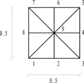
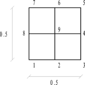
(a)	(b)	(c)

Figure 5. Patch used for sample problem; (a) Union Jack pattern, (b) Four square elements as the basic patch, (c) A square element as the basic patch.

Solution with triangular elements

A mesh of infinite dimensions is considered with a repeatable pattern in which the smallest unit is of form as the patch shown in Figure 5-a. After assembling the stiffness matrix of a macro patch of ${\textstyle 2\times 2}$ from the smallest unit, condensing the matrix for independent nodal values and also imposing the proportionality conditions similar to relations (52), the following expression for ${\textstyle {\boldsymbol {Q^{'}}}}$ is obtained

${\boldsymbol {Q^{'}}}\left({\mu }_{1},{\mu }_{2}\right)=$ $\left[{\begin{array}{ccc}4&-1-{\frac {1}{{\mu }_{1}}}&-1-{\frac {1}{{\mu }_{2}}}\\-1-{\mu }_{1}&{\frac {7}{2}}-{\frac {1}{4{\mu }_{2}}}-{\frac {{\mu }_{2}}{4}}&-{\frac {1}{4}}-{\frac {{\mu }_{1}}{4}}-{\frac {1}{4{\mu }_{2}}}-{\frac {{\mu }_{1}}{4{\mu }_{2}}}\\-1-{\mu }_{2}&-{\frac {1}{4}}-{\frac {1}{4{\mu }_{1}}}-{\frac {{\mu }_{2}}{4}}-{\frac {{\mu }_{2}}{4{\mu }_{1}}}&{\frac {7}{2}}-{\frac {1}{4{\mu }_{1}}}-{\frac {{\mu }_{1}}{4}}\end{array}}\right]$

The determinant of ${\textstyle {\boldsymbol {Q^{'}}}}$ is set to be zero and thus the characteristic equation is obtained as

$f\left({\mu }_{1},{\mu }_{2}\right)=33+{\frac {1}{4}}\left({\mu }_{1}^{2}+\right.$ $\left.{\mu }_{2}^{2}+{\mu }_{1}^{-2}+{\mu }_{2}^{-2}\right)-$ $8\left({\mu }_{1}+{\mu }_{2}+{\mu }_{1}^{-1}+{\mu }_{2}^{-1}\right)-$ ${\frac {1}{2}}\left({\mu }_{1}{\mu }_{2}+{\mu }_{1}^{-1}{\mu }_{2}+\right.$ $\left.{\mu }_{1}{\mu }_{2}^{-1}+{\mu }_{1}^{-1}{\mu }_{2}^{-1}\right)=$ $0$

We evaluate ${\textstyle {\mu }_{2}}$ in terms of ${\textstyle {\mu }_{1}}$

{\mu }_{2}=g_{1}({\mu }_{1})={\frac {1}{2}}\left(16+{\mu }_{1}^{-1}-8{\mu }_{1}^{-{\frac {1}{2}}}-8{\mu }_{1}^{\frac {1}{2}}+{\mu }_{1}-{\mu }_{1}^{-1}\left(-1+5{\mu }_{1}^{\frac {1}{2}}-5{\mu }_{1}+{\mu }_{1}^{\frac {3}{2}}\right){\left(1-6{\mu }_{1}^{\frac {1}{2}}+{\mu }_{1}\right)}^{\frac {1}{2}}\right)

${\mu }_{2}=g_{2}\left({\mu }_{1}\right)={\frac {1}{2}}\left(16+{\mu }_{1}^{-1}+8{\mu }_{1}^{-{\frac {1}{2}}}+8{\mu }_{1}^{\frac {1}{2}}+{\mu }_{1}-{\mu }_{1}^{-1}\left(1+5{\mu }_{1}^{\frac {1}{2}}+5{\mu }_{1}+{\mu }_{1}^{\frac {3}{2}}\right){\left(1+6{\mu }_{1}^{\frac {1}{2}}+{\mu }_{1}\right)}^{\frac {1}{2}}\right)$

${\mu }_{2}=g_{3}\left({\mu }_{1}\right)=g_{1}{\left({\mu }_{1}\right)}^{-1},{\mbox{ }}{\mu }_{2}=g_{4}\left({\mu }_{2}\right)=g_{2}{\left({\mu }_{1}\right)}^{-1}$

Similar expressions may be derived for ${\textstyle {\mu }_{1}}$ in terms of ${\textstyle {\mu }_{2}}$ . Generally, such explicit relations are not necessary and what needed is just choosing a value for ${\textstyle {\mu }_{1}}$ , as an integration point in the feasible domain, and solving an algebraic equation for its roots. Nevertheless, to give some insight to the problem the explicit relations are given here. Now we define

,

when ${\textstyle \vert {\mu }_{1}\vert \leq 1}$ . Similar functions are defined, with analogy, when ${\textstyle {\mu }_{1}}$ is evaluated in terms of ${\textstyle {\mu }_{2}}$ .

We should note that generally all quantities may take complex values, however, as pointed out before we take real values for one parameter and calculate the other one which may be in the form of a complex pair.

To give a finite element solution, we take exact fluxes normal to boundaries at ${\textstyle x=0}$ and ${\textstyle y=0}$ as tractions for the infinite domain to be solved. We note that although relations (87) or (88) may be employed to first find the unknown nodal boundary values and then extend the result to the interior parts through Equation (73) , one may directly use Equation (84) instead. Figure 6 depicts the variation of the finite element solution for ${\textstyle u}$ obtained from the proposed method using 10 patches along each axis, ${\textstyle x=0}$ and ${\textstyle y=0}$ . In order to show that the solution is close to an approximate finite element solution, in Figure 7 we give the results of a finite element solution on a domain of ${\textstyle 10\times 10}$ patches using exact fluxes for the other two boundaries. Although we do not expect that the two sets of results be identical, due to the fact that the tractions used for the latter finite element solution do not represent the tractions of remaining domain in FEM sense, the results are very close (the reader may also note that since all the boundary conditions for the latter solution are in Neumann form one node of the domain should be restrained, the most remote one in this case, thus this constitutes another source for the difference between the two sets of results). It can clearly be seen that the method proposed is able to give a finite element solution for a domain with unbounded dimension exhibiting a decay property.


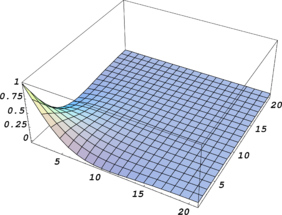
(a)	(b)

Figure 6. Finite solution obtained from the proposed method for the sample problem using ${\textstyle 10\times 10}$ patches with Union Jack pattern in Fig. 5-a and Neumann boundary condition at ${\textstyle x=0}$ and ${\textstyle y=0}$ ; (a) Contour line presentation, (b) Three dimensional plot presentation with horizontal axes scaled with element size.


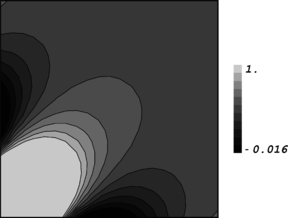
(a)	(b)

Figure 7. Standard finite solution for the sample problem using ${\textstyle 10\times 10}$ patches with Union Jack pattern in Fig. 5-a and Neumann boundary condition at ${\textstyle x=0}$ and ${\textstyle y=0}$ , and other two boundaries; (a) Contour line presentation, (b) Three dimensional plot presentation with horizontal axes scaled with element size.

The accuracy of the solution may be increased or decreased by use of different number of patches along the two axes. Figures 8 and 9 show the variation of ${\textstyle u}$ over the domain using different number of patches along each direction.


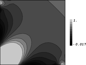
(a)	(b)

Figure 8. Finite solution obtained from the proposed method for the sample problem using ${\textstyle 8\times 8}$ patches with Union Jack pattern in Fig. 5-a and Neumann boundary condition at ${\textstyle x=0}$ and ${\textstyle y=0}$ . The results are shown on ${\textstyle 10\times 10}$ patches; (a) Contour line presentation, (b) Three dimensional plot presentation with horizontal axes scaled with element size.


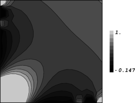
(a)	(b)

Figure 9. Finite solution obtained from the proposed method for the sample problem using ${\textstyle 6\times 6}$ patches with Union Jack pattern in Fig. 5-a and Neumann boundary condition at ${\textstyle x=0}$ and ${\textstyle y=0}$ . The results are shown on ${\textstyle 10\times 10}$ patches; (a) Contour line presentation, (b) Three dimensional plot presentation with horizontal axes scaled with element size.

Figure 10 also show the convergence of the results in terms of the number of integration points and patches used. In these figures the nodal values obtained for nodes 1 and 5 of the corner patch in Figure 4-b are plotted against the number of Gauss points and patches used. At the first glimpse no uniform convergence is seen, however, more careful look into the results reveals that the two values for nodes 1 and 5 follow each other with constant difference. The reason for such behavior lies in the rigid body motion of the whole sub-domain. We notice that the boundary conditions used are of Neumann type and no explicit essential condition is used except for the decay condition the strength of which varies between different solutions. The gradients and relative values show excellent convergence for moderate number of Gauss points and patches as shown in Figure 10 for ${\textstyle u_{5}-u_{1}}$ and ${\textstyle {\sigma }_{x}}$ , the gradient at center of element 1-2-9 in Figure 5-a.


(a)	(b)

Figure 10. Convergence of the solution with Neumann boundary condition- ${\textstyle u_{1}}$ and ${\textstyle u_{5}}$ are nodal values of node one and five in Union Jack Pattern of Fig 5-a for the corner patch of the domain, and ${\textstyle \sigma }$ is the gradient at center of triangle 1-2-9; (a) Convergence with respect to the number of Gauss points in a ${\textstyle 10\times 10}$ macro patch, (b) Convergence of solution with respect to the number of patches used along each direction while the number of Gauss points is fixed to 30 for all solutions.

We now examine the performance of the method when Dirichlet type of boundary conditions is of concern. The exact values are taken as prescribed boundary conditions along ${\textstyle x=0}$ and ${\textstyle y=0}$ . Equation (73) is directly employed to obtain the solution. To give a finite element solution for comparison, here again a square domain is solved with the prescribed values, at ${\textstyle x=0}$ and ${\textstyle y=0}$ , and Neumann boundary conditions at the other two edges. The results of the two solutions are presented in Figures 11 and 12. It can again be seen that the proposed method is able to produce the finite element solution. Figure 13 depicts the convergence of the proposed solution, in terms of the number of integration points and patches used. Unlike the case for Neumann boundary conditions, in this case uniform and fast convergence is seen in the results.


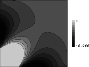
(a)	(b)

Figure 11. Finite solution obtained from the proposed method for the sample problem using ${\textstyle 10\times 10}$ patches with Union Jack pattern in Fig. 5-a and Dirichlet boundary condition at ${\textstyle x=0}$ and ${\textstyle y=0}$ ; (a) Contour line presentation, (b) Three dimensional plot presentation with horizontal axes scaled with element size.


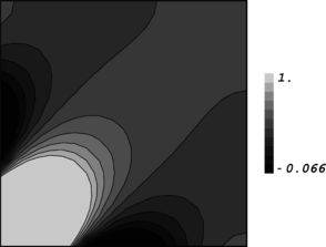
(a)	(b)

Figure 12. Standard finite solution for the sample problem using ${\textstyle 10\times 10}$ patches with Union Jack pattern in Fig. 5-a and Dirichlet boundary condition at ${\textstyle x=0}$ and ${\textstyle y=0}$ , and Neumann condition at the other two boundaries; (a) Contour line presentation, (b) Three dimensional plot presentation with horizontal axes scaled with element size.


(a)	(b)

Figure 13. Convergence of the solution with Dirichlet boundary condition- ${\textstyle u_{1}}$ and ${\textstyle u_{5}}$ are nodal values of node one and five in Union Jack Pattern of Fig 5-a for the corner patch of the domain, and ${\textstyle \sigma }$ is the gradient at center of triangle 1-2-9; (a) Convergence with respect to the number of Gauss points in a ${\textstyle 10\times 10}$ macro patch, (b) Convergence of solution with respect to the number of patches used along each direction while the number of Gauss points is fixed to 30 for all solutions.

Solution with four node elements

A mesh consisting of repeated patterns of a four square element as a macro-patch shown in Figure 5-b is considered for solution. Applying the proportionality relations, as (52), the following expression for the characteristic equation is obtained

$f\left({\mu }_{1},{\mu }_{2}\right)={\frac {799}{54}}-{\frac {259}{108}}F_{1}+$ ${\frac {25}{54}}F_{2}-{\frac {1}{108}}F_{3}-{\frac {49}{108}}F_{1}^{2}+$ ${\frac {1}{108}}F_{1}F_{2}-{\frac {1}{648}}F_{1}F_{3}+{\frac {1}{864}}F_{2}^{2}+$ ${\frac {1}{2592}}F_{1}^{4}$

Where

$F_{1}={\mu }_{1}+{\mu }_{1}^{-1}+{\mu }_{2}+{\mu }_{2}^{-1}$ , $F_{2}={\mu }_{1}^{2}+{\mu }_{1}^{-2}+{\mu }_{2}^{2}+{\mu }_{2}^{-2}$ , $F_{3}={\mu }_{1}^{3}+{\mu }_{1}^{-3}+{\mu }_{2}^{3}+{\mu }_{2}^{-3}$

From above characteristic equation ${\textstyle {\mu }_{2}}$ is to be calculated in terms of values given for ${\textstyle {\mu }_{1}}$ and vice versa. Two forms of problem, i.e. with Neumann and Dirichlet conditions, are solved using the proposed method. Some results obtained from using different numbers of patches along the axes are given in Figures 14 and 15. Once again, in order to compare the results with a standard finite element solution, a square domain is solved with the conditions mentioned previously, i.e. tractions from exact solution at all edges (see Figure 16). Convergence of the solution for one node of the domain is illustrated in Figure 17 in terms of number of integration points and patches used. Similar discussion as given for Figure 10 is valid here and as is seen the relative quantities and the gradients exhibit excellent convergence.


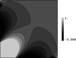
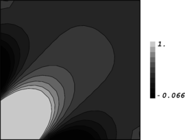
(a)	(b)

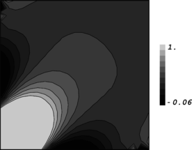
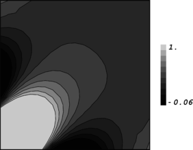
Figure 14. Contour plots for the finite solutions obtained from the proposed method for the sample problem using pattern of four squares in Fig. 5-b and Dirichlet boundary condition at ${\textstyle x=0}$ and ${\textstyle y=0}$ ; (a) Solution for ${\textstyle 8\times 8}$ patches shown on a domain of ${\textstyle 10\times 10}$ patches, (b) Solution for ${\textstyle 10\times 10}$ patches.


(a)	(b)

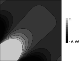
Figure 15. Contour plots the finite solutions obtained from the proposed method for the sample problem using pattern of four squares in Fig. 5-b and Neumann boundary condition at ${\textstyle x=0}$ and ${\textstyle y=0}$ ; (a) Solution for ${\textstyle 8\times 8}$ patches shown on a domain of ${\textstyle 10\times 10}$ patches, (b) Solution for ${\textstyle 10\times 10}$ patches.


(a)	(b)

Figure 16. Contour plots for standard finite solutions for the sample problem using ${\textstyle 10\times 10}$ pattern of four squares in Fig. 5-b and boundary condition at ${\textstyle x=0}$ and ${\textstyle y=0}$ ; (a) Neumann condition, (b) Dirichlet condition.


(a)	(b)

(c)	(d)

Figure 17. Convergence of the solution with Neumann and Dirichlet boundary condition- ${\textstyle u_{1}}$ and ${\textstyle u_{5}}$ are nodal values of node one and five in Fig 5-b for the corner patch of the domain, and ${\textstyle \sigma }$ is the gradient at center of element 1-2-9-8; (a)/(c) Convergence of solution with respect to the number of Gauss points in a ${\textstyle 10\times 10}$ macro patch, (b)/(d) Convergence of solution with respect to the number of patches used along each direction while the number of Gauss points is fixed to 30 for all solutions.

It is interesting to note that for solution using square elements, the smallest repeatable pattern may be considered as one element. Therefore, it is worthwhile to compare the results from such a solution with those obtained above.

If the proportionality conditions are written for one element, just one relation is obtained for ${\textstyle {\boldsymbol {Q^{'}}}}$ which is identical to the characteristic equation

$f\left({\mu }_{1},{\mu }_{2}\right)={\frac {1}{3}}\left[8-\right.$ $\left.\left({\mu }_{1}+{\mu }_{1}^{-1}+{\mu }_{2}+{\mu }_{2}^{-1}+\right.\right.$ $\left.\left.{\mu }_{1}{\mu }_{2}+{\mu }_{1}{\mu }_{2}^{-1}+\right.\right.$ $\left.\left.{\mu }_{1}^{-1}{\mu }_{2}+{\mu }_{1}^{-1}{\mu }_{2}^{-1}\right)\right]$

Figures 18 to 20 show the results obtained. Here ${\textstyle 20\times 20}$ patches are used in order that the results be comparable with those of Figures 14,15 and 17. Study on the convergence of the solution, while comparing to the solution with ${\textstyle 2\times 2}$ elements, demonstrates a slower rate of convergence in terms of the number of Gauss points and a faster rate in terms of the number of patches used (Figure 20).


(a)	(b)

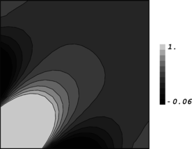
Figure 18. Contour plots for the finite solutions obtained from the proposed method for the sample problem using pattern of one square element in Fig. 5-c and Dirichlet boundary condition at ${\textstyle x=0}$ and ${\textstyle y=0}$ ; (a) Solution for ${\textstyle 16\times 16}$ patches shown on a domain of ${\textstyle 20\times 20}$ patches, (b) Solution for ${\textstyle 20\times 20}$ patches.


(a)	(b)

Figure 19. Contour plots for the finite solutions obtained from the proposed method for the sample problem using pattern of one square element in Fig. 5-c and Neumann boundary condition at ${\textstyle x=0}$ and ${\textstyle y=0}$ ; (a) Solution for ${\textstyle 16\times 16}$ patches shown on a domain of ${\textstyle 20\times 20}$ patches, (b) Solution for ${\textstyle 20\times 20}$ patches.


(a)	(b)

(c)	(d)

Figure 20. Convergence of the solution with Neumann and Dirichlet boundary condition- ${\textstyle u_{1}}$ and ${\textstyle u_{5}}$ are nodal values of node one and five in Fig 5-c for the corner patch of the domain, and ${\textstyle \sigma }$ is the gradient at center of element 1-2-3-4; (a)/(c) Convergence of solution with respect to the number of Gauss points in a ${\textstyle 20\times 20}$ macro patch, (b)/(d) Convergence of solution with respect to the number of patches used along each direction while the number of Gauss points is fixed to 30 for all solutions.

5. CONCLUSIONS

The formulation introduced by Babuška and co workers [13], for assessment of error estimator near flat boundaries, has been extended to kinked boundaries. The new formulation given is suitable for study of either asymptotic behavior of a finite element solution near boundaries or general FEM solution for unbounded domains.

Asymptotic finite element solution consists of two main parts; one obtained from patches located at interior of the domain, and another obtained from a boundary layer solution irrespective of other boundaries at far ends of the domain. The latter part of the solution decays towards the interior of the domain and, in this respect, is similar to a finite element solution of an unbounded domain.

The proposed method is based on assuming proportionality relations between the finite element nodal values along two or three directions, when the mesh is of a repeatable pattern. Writing the equilibrium equations over a unit patch leads to a characteristic equation containing all proportionality factors from which one may be expressed in terms of the others. The boundary layer solution is obtained by integral of extended vectors arranged in spectral form from null space vectors of the equilibrium equations. The decay condition is then applied by defining a feasible domain for proportionality factors.

Performance of the method has been examined for solution of unbounded domains in order to ensure its applicability to producing asymptotic finite element solution in an assessment procedure. A sample problem has been solved using two forms of patterns to demonstrate the capability of the method in reproducing the boundary layer solution. The convergence of the procedure has been studied with respect to number of patches as well as the number of integration points used. The results show fast convergence for both cases.

In the next part of the paper we shall give the step by step procedure for robustness test followed by numerous results obtained from application of the test to some recovery based error estimators.

APPENDIX

In this appendix we explain the reason for existence of proportionality property used in (52-a) to (52-c).

Integral Equation (27) may be viewed as a finite element solution of a corresponding differential equation with constant coefficient as the following one

on

(A-1)

For scalar problems such as heat conduction ones, for instance, the differential equation becomes

(A-2)

forgetting the subscript and superscripts for simplicity. Since the equation is of constant coefficient type, the solution may be expressed in an exponential form as ${\textstyle u=ce^{\alpha x+\beta y}}$ . This leads to a characteristic equation as ${\textstyle {\alpha }^{2}+{\beta }^{2}=0}$ after substitution in the equation. The exponential form of solution of (A-2) may be written as (see also [17])

(A-3)

or

(A-4)

where integrations are taken on feasible domain of ${\textstyle \alpha }$ or ${\textstyle \beta }$ , e.g. conditions for decay property. Considering single solution from (A-3) for example, it may be seen that the following relations exist

Similarly

or more generally

$u_{\left(x+nL_{x},y+mL_{y}\right)}=c_{\left(\alpha \right)}e^{\alpha (x+nL_{x})+\beta (y+mL_{y})}=$ ${\left({\mu }_{01}\right)}^{n}{\left({\mu }_{02}\right)}^{m}u_{\left(x,y\right)}$

Which is consistent with assumption made in (52-a) to (52-c). We note that here the differential equation is satisfied exactly whereas in relations (52) the aim is to satisfy the integral form of the equation. Of course the proportionality factors in the two approaches are not similar since one is an approximate finite element solution of another.

An important observation may be made by looking in to the characteristic equation ${\textstyle {\alpha }^{2}+{\beta }^{2}=0}$ . It can be seen that for a given value of ${\textstyle \alpha }$ there will be two values for ${\textstyle \beta }$ one of which corresponds to decay condition, i.e. ${\textstyle e^{-i\alpha y}}$ or ${\textstyle e^{i\alpha y}}$ (note that ${\textstyle \alpha }$ can be a complex value). Hence for a given value of ${\textstyle {\mu }_{01}}$ , two values as ${\textstyle {\mu }_{02}}$ and ${\textstyle {\mu }_{02}^{-1}}$ are both feasible but the one with absolute value less than unity corresponds to decay condition. Similar relations may be written for a general three dimensional problem.

References

[1] Oden, J.T., Belytschko, T., Babuška, I. and Hughes, T.J.R., “Research directions in computational mechanics” Comput. Methods Appl. Mech. Eng., Vol. 192, pp. 913-922, 2003.

[2] Zienkiewicz, O.C., “Achievements and some unsolved problems of finite element method” , Int. J. Numer. Meth. Engrg., Vol. 47, pp. 9-28, 2000.

[3] Hinton, E. and Campbell, J.S., “Local and global smoothing of discontinuous finite element functions using a least square method”, Int. J. Numer. Meth. Engrg., Vol. 8, pp. 461-480, 1976.

[4] Zienkiewicz, O.C. and Zhu, Z., “A simple error estimator and adaptivity procedure for practical engineering analysis”, Int. J. Numer. Meth. Engrg., Vol. 24, pp. 337-357, 1987.

[5] Tessler, A., Riggs, H.R. and Dambach, M., “A novel four-node quadrilateral smoothing element for stress enhancement and error estimation”, Int. J. Numer. Meth. Engrg., Vol. 44, pp. 1527-1543, 1999.

[6] Hiller, J.F. and Bathe, K.J., “On higher-order-accuracy points in isotropic finite element analysis and application to error assessment”, Comput. & Struc., Vol. 79, pp. 1275-1285, 2001.

[7] Zienkiewicz, O.C. and Zhu, Z., “The superconvergent patch recovery and a posteriori error estimates. Part II: Error estimates and adaptivity”, Int. J. Numer. Meth. Engrg., Vol. 33, pp. 1365-1382, 1992.

[8] Babuška, I., Strouboulis, T. and Upadhyay, C.S., “ A model study of the quality of a posteriori error estimaors for linear elliptic problems. Error estimation interior of patchwise uniform grids of triangles”, Comput. Methods Appl. Mech. Eng., Vol. 114, pp. 307-378, 1994.

[9] Babuška, I., Strouboulis, T., Upadhyay, C.S., Gangaraj, S.K. and Copps, K., “Validation of a posteriori error estimators by numerical approach”, Int. J. Numer. Meth. Engrg., Vol. 37, pp. 1073-1123, 1994.

[10] Babuška, I., Strouboulis, T., Upadhyay, C.S., Gangaraj, S.K. and Copps, K. “An objective criterion for assessing the reliability of a posteriori error estimators in finite element computations”, U.S.A.C.M. Bulletin, No.7 , pp. 4-16, 1994.

[11] Zhang, Z. and Zhang, S., “ Derivative superconvergence of rectangular finite elements for the Reissner-Mindlin plate”, Comput. Methods Appl. Mech. Eng., Vol. 134, pp. 1-16, 1996.

[12] Zhang, Z., “ Superconvergence in projected –shear plate-bending finite element methods”, Numer. Meth. Partial Diff. Eqn., Vol. 14, pp. 367-386, 1998.

[13] Babuška, I., Strouboulis, T. and Upadhyay, C.S., “A model study of the quality of a posteriori error estimators for finite element solutions of linear elliptic problems, with particular reference to the behavior near the boundary”, Int. J. Numer. Meth. Engrg., Vol. 40, pp. 2521-2577, 1997.

[14] Ainsworth, M. and Oden, J.T., A posteriori error estimation in finite element analysis, John Wiley, 2000.

[15] Zienkiewicz, O. C. and Taylor, R. L., “The finite element method”, 5^th edition, Butterworth-Heineman, 2000.

[16] Boroomand, B. and Zienkiewicz, O.C., “An improved REP recovery and efectivity robustness test”, Int. J. Numer. Meth. Engrg., Vol. 33, pp. 3247-3277, 1997.

[17] Hildebrand, F., Advanced calculus for applications, Second edition, Prentice-Hall, 1976.

Latest revision as of 12:50, 15 June 2018

Abstract

1. INTRODUCTION

2. PRELIMINARIES

3. ROBUSTNESS PATCH TEST

4. NUMERICAL PRESENTATION

5. CONCLUSIONS

APPENDIX

References

Document information

Document Score

Share this document

Keywords

claim authorship

@@ Line 189: / Line 189: @@
 {| style="text-align: center; margin:auto;"
 |-
-| <math display="inline">R=max\left(\vert 1-{\theta }_L\vert +\vert 1-{\theta }_U\vert ,\vert 1- \frac{1}{{\theta }_L}\vert +\vert 1-\frac{1}{{\theta }_U}\vert \right)</math>
+| <math>R=max\left(\vert 1-{\theta }_L\vert +\vert 1-{\theta }_U\vert ,\vert 1- \frac{1}{{\theta }_L}\vert +\vert 1-\frac{1}{{\theta }_U}\vert \right)</math>
 |}
 | style="width: 5px;text-align: right;white-space: nowrap;" | (8)
@@ Line 202: / Line 202: @@
 :* It is assumed that in all directions the mesh is locally uniform and is composed of a series of repeatable pasterns, as the basic cell with dimension  <math display="inline">h</math> especially inside  <math display="inline">{\Omega }_1</math> in Figure 1. A single cell of the repeatable pattern is considered as a patch for the test.  The reader may notice that such patches have different definitions from the ones used for recovery methods.  Note that no assumption is made about the mesh outside of  <math display="inline">{\Omega }_1</math>.
+{| style="width: 100%;border-collapse: collapse;"
+|-
+|  style="text-align: center;vertical-align: top;width: 51%;"| [[Image:draft_Samper_725107104-image429.png|270px]]
+|  style="vertical-align: top;width: 51%;"| [[Image:draft_Samper_725107104-image430.png|288px]]
+|-
+|  style="text-align: center;vertical-align: top;"|(a)
+|  style="text-align: center;vertical-align: top;"|(b)
+|}
+Figure 1.  The domain, subdomain and basic cell considered for robustness patch test; (a) Three  dimensional presentation of the domain; (b) Projection of the domain on a two dimensional plane.
 :* Study on asymptotic convergence of the solution requires that the elements sizes be close to zero and so the dimensions of patches consisting a number of such elements like patches shown in Figure 1, i.e. basic cell with dimension  <math display="inline">h</math> and the larger patches with dimensions  <math display="inline">h_0</math> and  <math display="inline">h_1</math> (<math display="inline">h_0</math> and  <math display="inline">h_1</math> are multiples of  <math display="inline">h</math>). In this regard it is also assumed that that  <math display="inline">h</math> tends to zero with a faster rate than  <math display="inline">h_0</math> (and  <math display="inline">h_1</math>). Moreover, it is assumed that the basic cells are cuboid (in three dimensions) with edges parallel to axes, though this is not necessary in general.
@@ Line 224: / Line 238: @@
 {| style="text-align: center; margin:auto;"
 |-
-| <math display="inline">u_{ex}=a_0+a_1\Delta x+a_2\Delta y+a_3\Delta z+\cdots +</math><math>a_{10}\Delta x^3+a_{11}\Delta x\Delta y^2+a_{12}\Delta x\Delta y\Delta z+</math><math>\cdots </math>
+| <math>u_{ex}=a_0+a_1\Delta x+a_2\Delta y+a_3\Delta z+\cdots +</math><math>a_{10}\Delta x^3+a_{11}\Delta x\Delta y^2+a_{12}\Delta x\Delta y\Delta z+</math><math>\cdots </math>
 |}
 | style="width: 5px;text-align: right;white-space: nowrap;" | (9)
@@ Line 237: / Line 251: @@
 {| style="text-align: center; margin:auto;"
 |-
-| <math display="inline">u_{ex}=\boldsymbol{p}^T\boldsymbol{a}</math> ,           <math display="inline">\boldsymbol{p}=\langle X^{p+1},X^PY,\cdots X^lY^mZ^n,\cdots \rangle </math> , <math display="inline">\boldsymbol{a}={\langle a_1,a_2,\cdots \cdots \rangle }^T</math> ,      <math display="inline">l+m+n=p+1</math> .
+| <math>u_{ex}=\boldsymbol{p}^T\boldsymbol{a}</math> ,           <math>\boldsymbol{p}=\langle X^{p+1},X^PY,\cdots X^lY^mZ^n,\cdots \rangle </math> , <math display="inline">\boldsymbol{a}={\langle a_1,a_2,\cdots \cdots \rangle }^T</math> ,      <math>l+m+n=p+1</math> .
 |}
 | style="width: 5px;text-align: right;white-space: nowrap;" | (10)
@@ Line 250: / Line 264: @@
 {| style="text-align: center; margin:auto;"
 |-
-| <math display="inline">\boldsymbol{u}_{ex}=\sum_{i=1}^3(\boldsymbol{p}^T\boldsymbol{a}_i)\boldsymbol{1}_i</math> ,              <math display="inline">\boldsymbol{p}=\langle X^2,Y^2,Z^2,XY,YZ,XZ\rangle </math> ,  <math display="inline">\boldsymbol{a}_i={\langle a_{6i-5},a_{6i-4},a_{6i-3},a_{6i-2},a_{6i-1},a_{6i}\rangle }^T</math>
+| <math>\boldsymbol{u}_{ex}=\sum_{i=1}^3(\boldsymbol{p}^T\boldsymbol{a}_i)\boldsymbol{1}_i</math> ,              <math>\boldsymbol{p}=\langle X^2,Y^2,Z^2,XY,YZ,XZ\rangle </math> ,  <math>\boldsymbol{a}_i={\langle a_{6i-5},a_{6i-4},a_{6i-3},a_{6i-2},a_{6i-1},a_{6i}\rangle }^T</math>
 |}
 | style="width: 5px;text-align: right;white-space: nowrap;" | (11)
@@ Line 271: / Line 285: @@
 {| style="text-align: center; margin:auto;"
 |-
-| <math display="inline">\boldsymbol{u}_{ex}=\boldsymbol{N}{\boldsymbol{\overline{u}}}_{ex}+</math><math>\left(\boldsymbol{u}_{ex}-\boldsymbol{N}{\boldsymbol{\overline{u}}}_{ex}\right)</math>
+| <math>\boldsymbol{u}_{ex}=\boldsymbol{N}{\boldsymbol{\overline{u}}}_{ex}+</math><math>\left(\boldsymbol{u}_{ex}-\boldsymbol{N}{\boldsymbol{\overline{u}}}_{ex}\right)</math>
 |}
 | style="width: 5px;text-align: right;white-space: nowrap;" | (12)
@@ Line 284: / Line 298: @@
 {| style="text-align: center; margin:auto;"
 |-
-| <math display="inline">\left({\int }_{\mbox{ }\mbox{ }\Omega }\boldsymbol{B}^T\boldsymbol{DB}\mbox{ }d\Omega \right)\left({\boldsymbol{\overline{u}}}_h- {\boldsymbol{\overline{u}}}_{ex}\right)= </math><math> {\int }_{\mbox{ }\mbox{ }\Omega }\boldsymbol{B}^T\boldsymbol{DS}\left(\boldsymbol{u}_{ex}- \boldsymbol{N}{\boldsymbol{\overline{u}}}_{ex}\right)\mbox{ }d\Omega </math>
+| <math>\left({\int }_{\mbox{ }\mbox{ }\Omega }\boldsymbol{B}^T\boldsymbol{DB}\mbox{ }d\Omega \right)\left({\boldsymbol{\overline{u}}}_h- {\boldsymbol{\overline{u}}}_{ex}\right)= </math><math> {\int }_{\mbox{ }\mbox{ }\Omega }\boldsymbol{B}^T\boldsymbol{DS}\left(\boldsymbol{u}_{ex}- \boldsymbol{N}{\boldsymbol{\overline{u}}}_{ex}\right)\mbox{ }d\Omega </math>
 |}
 | style="width: 5px;text-align: right;white-space: nowrap;" | (13)
@@ Line 299: / Line 313: @@
 {| style="text-align: center; margin:auto;"
 |-
-| <math display="inline">\left({\int }_{\mbox{ }{\Omega }^{{'}}}\boldsymbol{B}^T\boldsymbol{DB}\mbox{ }\mbox{ }d\Omega \right){\boldsymbol{\overline{u}}}_h^p=</math><math>{\int }_{\mbox{ }{\Omega }^{{'}}}\boldsymbol{B}^T\boldsymbol{DS}\left(\boldsymbol{u}_{ex}-\right. </math><math>\left. \boldsymbol{N}{\boldsymbol{\overline{u}}}_{ex}\right)\mbox{ }\mbox{ }d\Omega </math>
+| <math>\left({\int }_{\mbox{ }{\Omega }^{{'}}}\boldsymbol{B}^T\boldsymbol{DB}\mbox{ }\mbox{ }d\Omega \right){\boldsymbol{\overline{u}}}_h^p=</math><math>{\int }_{\mbox{ }{\Omega }^{{'}}}\boldsymbol{B}^T\boldsymbol{DS}\left(\boldsymbol{u}_{ex}-\right. </math><math>\left. \boldsymbol{N}{\boldsymbol{\overline{u}}}_{ex}\right)\mbox{ }\mbox{ }d\Omega </math>
 |}
 | style="width: 5px;text-align: right;white-space: nowrap;" | (14)
@@ Line 313: / Line 327: @@
 {| style="text-align: center; margin:auto;"
 |-
-| <math display="inline">{\boldsymbol{\overline{u}}}_h={\boldsymbol{\overline{u}}}_{ex}+</math><math>{\boldsymbol{\overline{u}}}_h^p+\boldsymbol{C}</math>
+| <math>{\boldsymbol{\overline{u}}}_h={\boldsymbol{\overline{u}}}_{ex}+</math><math>{\boldsymbol{\overline{u}}}_h^p+\boldsymbol{C}</math>
 |}
 | style="width: 5px;text-align: right;white-space: nowrap;" | (15)
@@ Line 326: / Line 340: @@
 {| style="text-align: center; margin:auto;"
 |-
-| <math display="inline">{\int }_{\mbox{ }{\Omega }^{{'}}}(\boldsymbol{N}{\boldsymbol{\overline{u}}}_h^p+</math><math>\boldsymbol{C})\mbox{ }\mbox{ }d\Omega ={\int }_{\mbox{ }{\Omega }^{{'}}}(\boldsymbol{u}_{ex}-</math><math>\boldsymbol{N}{\boldsymbol{\overline{u}}}_{ex})\mbox{ }d\Omega </math>
+| <math>{\int }_{\mbox{ }{\Omega }^{{'}}}(\boldsymbol{N}{\boldsymbol{\overline{u}}}_h^p+</math><math>\boldsymbol{C})\mbox{ }\mbox{ }d\Omega ={\int }_{\mbox{ }{\Omega }^{{'}}}(\boldsymbol{u}_{ex}-</math><math>\boldsymbol{N}{\boldsymbol{\overline{u}}}_{ex})\mbox{ }d\Omega </math>
 |}
 | style="width: 5px;text-align: right;white-space: nowrap;" | (16)
@@ Line 339: / Line 353: @@
 {| style="text-align: center; margin:auto;"
 |-
-| <math display="inline">{\Vert \boldsymbol{e}_{\boldsymbol{\sigma }}\Vert }_{L_2,{\Omega }^{{'}}}^2=</math><math>{\int }_{\mbox{ }{\Omega }^{{'}}}{\left({\boldsymbol{\sigma }}_{ex}-{\boldsymbol{\sigma }}_h\right)}^T\left({\boldsymbol{\sigma }}_{ex}-\right. </math><math>\left. {\boldsymbol{\sigma }}_h\right)\mbox{ }d\Omega =</math><math>\boldsymbol{a}^T\boldsymbol{E}_0\boldsymbol{a}</math>
+| <math>{\Vert \boldsymbol{e}_{\boldsymbol{\sigma }}\Vert }_{L_2,{\Omega }^{{'}}}^2=</math><math>{\int }_{\mbox{ }{\Omega }^{{'}}}{\left({\boldsymbol{\sigma }}_{ex}-{\boldsymbol{\sigma }}_h\right)}^T\left({\boldsymbol{\sigma }}_{ex}-\right. </math><math>\left. {\boldsymbol{\sigma }}_h\right)\mbox{ }d\Omega =</math><math>\boldsymbol{a}^T\boldsymbol{E}_0\boldsymbol{a}</math>
 |}
 | style="width: 5px;text-align: right;white-space: nowrap;" | (17)
@@ Line 352: / Line 366: @@
 {| style="text-align: center; margin:auto;"
 |-
-| <math display="inline">{\Vert \boldsymbol{e}_{\boldsymbol{\sigma }}^\ast \Vert }_{L_2,{\Omega }^{{'}}}^2=</math><math>\boldsymbol{a}^T\boldsymbol{Ea}</math>
+| <math>{\Vert \boldsymbol{e}_{\boldsymbol{\sigma }}^\ast \Vert }_{L_2,{\Omega }^{{'}}}^2=</math><math>\boldsymbol{a}^T\boldsymbol{Ea}</math>
 |}
 | style="width: 5px;text-align: right;white-space: nowrap;" | (18)
@@ Line 378: / Line 392: @@
 {| style="text-align: center; margin:auto;"
 |-
-| <math display="inline">\boldsymbol{\tilde{E}}=\boldsymbol{H}^{-T}\boldsymbol{E}\boldsymbol{H}^{-1}</math>
+| <math>\boldsymbol{\tilde{E}}=\boldsymbol{H}^{-T}\boldsymbol{E}\boldsymbol{H}^{-1}</math>
 |}
 | style="width: 5px;text-align: right;white-space: nowrap;" | (20)
@@ Line 404: / Line 418: @@
 {| style="text-align: center; margin:auto;"
 |-
-| <math display="inline">{\left({\lambda }_{min}\right)}^{\frac{1}{2}}<\theta <{\left({\lambda }_{max}\right)}^{\frac{1}{2}}</math> ,               <math display="inline">{\theta }_L={\left({\lambda }_{min}\right)}^{\frac{1}{2}}</math> ,             <math display="inline">{\theta }_U={\left({\lambda }_{max}\right)}^{\frac{1}{2}}</math>
+| <math>{\left({\lambda }_{min}\right)}^{\frac{1}{2}}<\theta <{\left({\lambda }_{max}\right)}^{\frac{1}{2}}</math> , <math>{\theta }_L={\left({\lambda }_{min}\right)}^{\frac{1}{2}}</math> ,  <math>{\theta }_U={\left({\lambda }_{max}\right)}^{\frac{1}{2}}</math>
 |}
 | style="width: 5px;text-align: right;white-space: nowrap;" | (22)
@@ Line 421: / Line 435: @@
 {| style="text-align: center; margin:auto;"
 |-
-| <math display="inline">\left({\int }_{\mbox{ }{\Omega }_p}\boldsymbol{B}^T\boldsymbol{DB}\mbox{ }\mbox{ }d\Omega \right){\boldsymbol{\overline{u}}}_h^p=</math><math>{\int }_{\mbox{ }{\Omega }_p}\boldsymbol{B}^T\boldsymbol{DS}\left(\boldsymbol{u}_{ex}- \boldsymbol{N}{\boldsymbol{\overline{u}}}_{ex}\right)\mbox{ }d\Omega </math>
+| <math>\left({\int }_{\mbox{ }{\Omega }_p}\boldsymbol{B}^T\boldsymbol{DB}\mbox{ }\mbox{ }d\Omega \right){\boldsymbol{\overline{u}}}_h^p=</math><math>{\int }_{\mbox{ }{\Omega }_p}\boldsymbol{B}^T\boldsymbol{DS}\left(\boldsymbol{u}_{ex}- \boldsymbol{N}{\boldsymbol{\overline{u}}}_{ex}\right)\mbox{ }d\Omega </math>
 |}
 | style="width: 5px;text-align: right;white-space: nowrap;" | (23)
@@ Line 437: / Line 451: @@
 {|
 |-
-| <math display="inline">{\boldsymbol{\overline{u}}}_{h(X+L_x)}^p={\boldsymbol{\overline{u}}}_{h(X)}^p</math>
+| <math>{\boldsymbol{\overline{u}}}_{h(X+L_x)}^p={\boldsymbol{\overline{u}}}_{h(X)}^p</math>
-| <math display="inline">{\boldsymbol{\overline{u}}}_{h(Y+L_y)}^p={\boldsymbol{\overline{u}}}_{h(Y)}^p</math>
+| <math>{\boldsymbol{\overline{u}}}_{h(Y+L_y)}^p={\boldsymbol{\overline{u}}}_{h(Y)}^p</math>
 |}
-<math display="inline">{\boldsymbol{\overline{u}}}_{h(Z+L_z)}^p={\boldsymbol{\overline{u}}}_{h(Z)}^p</math>
+<math>{\boldsymbol{\overline{u}}}_{h(Z+L_z)}^p={\boldsymbol{\overline{u}}}_{h(Z)}^p</math>
 |}
 | style="width: 5px;text-align: right;white-space: nowrap;" | (24)
@@ Line 457: / Line 471: @@
 {| style="text-align: center; margin:auto;"
 |-
-| <math display="inline">\left({\int }_{\mbox{ }{\Omega }^{{'}}}\boldsymbol{B}^T\boldsymbol{DB}\mbox{ }\mbox{ }d\Omega \right){\boldsymbol{\overline{u}}}_{hB}^p=</math><math>{\int }_{\mbox{ }{\Omega }^{{'}}}\boldsymbol{B}^T\boldsymbol{DS}\left(\boldsymbol{u}_{ex}- \boldsymbol{N}{\boldsymbol{\overline{u}}}_{ex}\right)\mbox{ }d\Omega </math>
+| <math>\left({\int }_{\mbox{ }{\Omega }^{{'}}}\boldsymbol{B}^T\boldsymbol{DB}\mbox{ }\mbox{ }d\Omega \right){\boldsymbol{\overline{u}}}_{hB}^p=</math><math>{\int }_{\mbox{ }{\Omega }^{{'}}}\boldsymbol{B}^T\boldsymbol{DS}\left(\boldsymbol{u}_{ex}- \boldsymbol{N}{\boldsymbol{\overline{u}}}_{ex}\right)\mbox{ }d\Omega </math>
 |}
 | style="width: 5px;text-align: right;white-space: nowrap;" | (25)
@@ Line 483: / Line 497: @@
 {| style="text-align: center; margin:auto;"
 |-
-| <math display="inline">\left({\int }_{\mbox{ }\mbox{ }{\Omega }^{{'}}}\boldsymbol{B}^T\boldsymbol{DB}\mbox{ }\mbox{ }d\Omega \right){\boldsymbol{\overline{u}}}_{h0}^p=\boldsymbol{0}\mbox{ }\mbox{ }\mbox{on }\mbox{ }{\Omega }^{{'}}</math>
+| <math>\left({\int }_{\mbox{ }\mbox{ }{\Omega }^{{'}}}\boldsymbol{B}^T\boldsymbol{DB}\mbox{ }\mbox{ }d\Omega \right){\boldsymbol{\overline{u}}}_{h0}^p=\boldsymbol{0}\mbox{ }\mbox{ }\mbox{on }\mbox{ }{\Omega }^{{'}}</math>
 |}
 | style="width: 5px;text-align: right;white-space: nowrap;" | (27)
@@ Line 496: / Line 510: @@
 {| style="text-align: center; margin:auto;"
 |-
-| <math display="inline">{\boldsymbol{\overline{u}}}_{h0}^p\rightarrow 0</math> (or  <math display="inline">\boldsymbol{B}{\boldsymbol{\overline{u}}}_{h0}^p\rightarrow 0</math> )       when      <math display="inline">\frac{d_z}{L_z}\rightarrow \infty </math>
+| <math>{\boldsymbol{\overline{u}}}_{h0}^p\rightarrow 0</math> (or  <math>\boldsymbol{B}{\boldsymbol{\overline{u}}}_{h0}^p\rightarrow 0</math> )       when      <math>\frac{d_z}{L_z}\rightarrow \infty </math>
 |}
 | style="width: 5px;text-align: right;white-space: nowrap;" | (28)
@@ Line 513: / Line 527: @@
 {| style="text-align: center; margin:auto;"
 |-
-| <math display="inline">{\boldsymbol{\overline{u}}}_h={\boldsymbol{\overline{u}}}_{ex}</math>
+| <math>{\boldsymbol{\overline{u}}}_h={\boldsymbol{\overline{u}}}_{ex}</math>
 |}
 | style="width: 5px;text-align: right;white-space: nowrap;" | (29)
@@ Line 526: / Line 540: @@
 {| style="text-align: center; margin:auto;"
 |-
-| <math display="inline">{\boldsymbol{\overline{u}}}_h={\boldsymbol{\overline{u}}}_{ex}+</math><math>{\boldsymbol{\overline{u}}}_{hB}^p</math>
+| <math>{\boldsymbol{\overline{u}}}_h={\boldsymbol{\overline{u}}}_{ex}+</math><math>{\boldsymbol{\overline{u}}}_{hB}^p</math>
 |}
 | style="width: 5px;text-align: right;white-space: nowrap;" | (30)
@@ Line 539: / Line 553: @@
 {| style="text-align: center; margin:auto;"
 |-
-| <math display="inline">{\boldsymbol{\overline{u}}}_{hB}^p\vert _{{\Gamma }_D}=</math><math>\boldsymbol{0}</math>
+| <math>{\boldsymbol{\overline{u}}}_{hB}^p\vert _{{\Gamma }_D}=</math><math>\boldsymbol{0}</math>
 |}
 | style="width: 5px;text-align: right;white-space: nowrap;" | (31)
@@ Line 552: / Line 566: @@
 {| style="text-align: center; margin:auto;"
 |-
-| <math display="inline">{\boldsymbol{\overline{u}}}_{h0}^p\vert _{{\Gamma }_D}=</math><math>-({\boldsymbol{\overline{u}}}_h^p+\boldsymbol{C})\vert _{{\Gamma }_D}</math>
+| <math>{\boldsymbol{\overline{u}}}_{h0}^p\vert _{{\Gamma }_D}=</math><math>-({\boldsymbol{\overline{u}}}_h^p+\boldsymbol{C})\vert _{{\Gamma }_D}</math>
 |}
 | style="width: 5px;text-align: right;white-space: nowrap;" | (32)
@@ Line 569: / Line 583: @@
 {| style="text-align: center; margin:auto;"
 |-
-| <math display="inline">\boldsymbol{t}_0=\boldsymbol{\tilde{n}DS}\boldsymbol{u}_{ex}</math>
+| <math>\boldsymbol{t}_0=\boldsymbol{\tilde{n}DS}\boldsymbol{u}_{ex}</math>
 |}
 | style="width: 5px;text-align: right;white-space: nowrap;" | (33)
@@ Line 582: / Line 596: @@
 {| style="text-align: center; margin:auto;"
 |-
-| <math display="inline">{\int }_{\mbox{ }\mbox{ }{\Omega }^{{'}}}\boldsymbol{B}^T\boldsymbol{DB}[{\boldsymbol{\overline{u}}}_{ex}+</math><math>({\boldsymbol{\overline{u}}}_h^p+\boldsymbol{C})+{\boldsymbol{\overline{u}}}_{h0}^p]\mbox{ }\mbox{ }d\Omega -</math><math>{\int }_{\mbox{ }\mbox{ }{\Omega }^{{'}}}\boldsymbol{N}^T\boldsymbol{b}\mbox{ }d\Omega -</math><math>{\int }_{\mbox{ }\mbox{ }{\Gamma }_t}\boldsymbol{N}^T\boldsymbol{t}_0\mbox{ }d\Gamma =</math><math>\boldsymbol{0}</math>
+| <math>{\int }_{\mbox{ }\mbox{ }{\Omega }^{{'}}}\boldsymbol{B}^T\boldsymbol{DB}[{\boldsymbol{\overline{u}}}_{ex}+</math><math>({\boldsymbol{\overline{u}}}_h^p+\boldsymbol{C})+{\boldsymbol{\overline{u}}}_{h0}^p]\mbox{ }\mbox{ }d\Omega -</math><math>{\int }_{\mbox{ }\mbox{ }{\Omega }^{{'}}}\boldsymbol{N}^T\boldsymbol{b}\mbox{ }d\Omega -</math><math>{\int }_{\mbox{ }\mbox{ }{\Gamma }_t}\boldsymbol{N}^T\boldsymbol{t}_0\mbox{ }d\Gamma =</math><math>\boldsymbol{0}</math>
 |}
 | style="width: 5px;text-align: right;white-space: nowrap;" | (34)
@@ Line 595: / Line 609: @@
 {| style="text-align: center; margin:auto;"
 |-
-| <math display="inline">\boldsymbol{b}=-\boldsymbol{S}^T\boldsymbol{DS}\boldsymbol{u}_{ex}</math>
+| <math>\boldsymbol{b}=-\boldsymbol{S}^T\boldsymbol{DS}\boldsymbol{u}_{ex}</math>
 |}
 | style="width: 5px;text-align: right;white-space: nowrap;" | (35)
@@ Line 621: / Line 635: @@
 {| style="text-align: center; margin:auto;"
 |-
-| <math display="inline">\left({\int }_{\mbox{ }{{\Omega }^{{'}}}_{bnd}}\boldsymbol{B}_{bnd}^T\boldsymbol{DB}\mbox{ }d\Omega \right){\left({\boldsymbol{\overline{u}}}_{h0}^p\right)}_{bnd}=\boldsymbol{F}_{prs}</math>
+| <math>\left({\int }_{\mbox{ }{{\Omega }^{{'}}}_{bnd}}\boldsymbol{B}_{bnd}^T\boldsymbol{DB}\mbox{ }d\Omega \right){\left({\boldsymbol{\overline{u}}}_{h0}^p\right)}_{bnd}=\boldsymbol{F}_{prs}</math>
 |}
 | style="width: 5px;text-align: right;white-space: nowrap;" | (37)
@@ Line 630: / Line 644: @@
 Now we are ready to apply the boundary condition to a problem asymptotically modeled with a periodic mesh pattern and a single flat boundary.   Considering a 3D mesh of patches like Figure 2-a, we assume that the boundary exists at plane  <math display="inline">z=0</math>.  The mesh pattern is considered repeatable along <math display="inline">x</math>, <math display="inline">y</math> and  <math display="inline">z</math>, with  <math display="inline">-\infty <x<\infty </math>,  <math display="inline">-\infty <y<\infty </math> and  <math display="inline">0<z<\infty </math>.  A column of patches along  <math display="inline">z</math> is selected.  For simplicity we use Figure 2-b instead of Figure 2-a as a two dimensional presentation of the three dimensional column.  Note that we are aiming at solving Equation (27) or (37) in which  <math display="inline">{\Omega }^{{'}}</math> is volume of the column.
+{| style="width: 100%;border-collapse: collapse;"
+|-
+|  style="vertical-align: top;width: 51%;"| [[Image:draft_Samper_725107104-image431.png|264px]]
+|  style="vertical-align: top;width: 51%;"| [[Image:draft_Samper_725107104-image432.png|312px]]
+|-
+|  style="text-align: center;vertical-align: top;"|(a)
+|  style="text-align: center;vertical-align: top;"|(b)
+|}
+Figure 2.  A column with infinite length; (a) Three dimensional presentation of the column with one end at boundary consisting of repeatable patterns as basic cells, (b)  Two dimensional presentation of the infinite column with repeatable pattern and the numbering used for different levels.
 After numbering the patch levels consecutively towards the middle of the domain as shown in Figure 2-b, in the matrix equation of each patch the degrees of freedoms not falling on interfaces of patches are statically condensed.  The matrix equation of the asymptotic finite element solution pertaining to the remaining degrees of freedoms is assembled as
@@ Line 678: / Line 705: @@
 {| style="text-align: center; margin:auto;"
 |-
-| <math display="inline">\left[\begin{array}{ccc}
+| <math>\left[\begin{array}{ccc}
 \boldsymbol{A} & \boldsymbol{B} & \boldsymbol{C}
 \end{array}\right]\cdot \left\{\begin{array}{c}
@@ Line 697: / Line 724: @@
 {| style="text-align: center; margin:auto;"
 |-
-| <math display="inline">\left[\begin{array}{cc}
+| <math>\left[\begin{array}{cc}
 \boldsymbol{A} & \boldsymbol{B}\\
 \boldsymbol{0} & \boldsymbol{I}
@@ Line 722: / Line 749: @@
 {| style="text-align: center; margin:auto;"
 |-
-| <math display="inline">\left\{\begin{array}{c}
+| <math>\left\{\begin{array}{c}
 {\boldsymbol{\overline{u}}}_{h0}^{p,n+1}\\
 {\boldsymbol{\overline{u}}}_{h0}^{p,n}
@@ Line 744: / Line 771: @@
 {| style="text-align: center; margin:auto;"
 |-
-| <math display="inline">\left\{\begin{array}{c}
+| <math>\left\{\begin{array}{c}
 {\boldsymbol{\overline{u}}}_{h0}^{p,n+1}\\
 {\boldsymbol{\overline{u}}}_{h0}^{p,n}
@@ Line 766: / Line 793: @@
 {| style="text-align: center; margin:auto;"
 |-
-| <math display="inline">\left(\left[\begin{array}{cc}
+| <math>\left(\left[\begin{array}{cc}
 \boldsymbol{A} & \boldsymbol{B}\\
 \boldsymbol{0} & \boldsymbol{I}
@@ Line 785: / Line 812: @@
 {| style="text-align: center; margin:auto;"
 |-
-| <math display="inline">\boldsymbol{w}_i^n={\mu }_i^{n-m}\boldsymbol{w}_i^m</math>
+| <math>\boldsymbol{w}_i^n={\mu }_i^{n-m}\boldsymbol{w}_i^m</math>
 |}
 | style="width: 5px;text-align: right;white-space: nowrap;" | (44)
@@ Line 829: / Line 856: @@
 {| style="text-align: center; margin:auto;"
 |-
-| <math display="inline">\boldsymbol{u}_h=\boldsymbol{N}\left({\boldsymbol{\overline{u}}}_{ex}+ {\boldsymbol{\overline{u}}}_h^p+{\boldsymbol{\overline{u}}}_{h0}^p+\right. </math><math>\left. \boldsymbol{C}\right)</math>
+| <math>\boldsymbol{u}_h=\boldsymbol{N}\left({\boldsymbol{\overline{u}}}_{ex}+ {\boldsymbol{\overline{u}}}_h^p+{\boldsymbol{\overline{u}}}_{h0}^p+\right. </math><math>\left. \boldsymbol{C}\right)</math>
 |}
 | style="width: 5px;text-align: right;white-space: nowrap;" | (47)
@@ Line 850: / Line 877: @@
 {| style="text-align: center; margin:auto;"
 |-
-| <math display="inline">\left({\int }_{\mbox{ }\mbox{ }{\Omega }^{{'}}}\boldsymbol{B}^T\boldsymbol{DB}\mbox{ }\mbox{ }d\Omega \right){\boldsymbol{\overline{u}}}_{hB}^p=</math><math>{\int }_{\mbox{ }\mbox{ }{\Omega }^{{'}}}\boldsymbol{B}^T\boldsymbol{DS}\left(\boldsymbol{u}_{ex}- \boldsymbol{N}{\boldsymbol{\overline{u}}}_{ex}\right)\mbox{ }d\Omega </math>
+| <math>\left({\int }_{\mbox{ }\mbox{ }{\Omega }^{{'}}}\boldsymbol{B}^T\boldsymbol{DB}\mbox{ }\mbox{ }d\Omega \right){\boldsymbol{\overline{u}}}_{hB}^p=</math><math>{\int }_{\mbox{ }\mbox{ }{\Omega }^{{'}}}\boldsymbol{B}^T\boldsymbol{DS}\left(\boldsymbol{u}_{ex}- \boldsymbol{N}{\boldsymbol{\overline{u}}}_{ex}\right)\mbox{ }d\Omega </math>
 |}
 | style="width: 5px;text-align: right;white-space: nowrap;" | (48)
 |}
+{| style="width: 100%;border-collapse: collapse;"
+|-
+|  style="vertical-align: top;width: 54%;"|                   [[Image:draft_Samper_725107104-image433.png|234px]]
+|  style="vertical-align: top;width: 47%;"|               [[Image:draft_Samper_725107104-image434.png|216px]]
+|-
+|  style="text-align: center;vertical-align: top;"|(a)
+|  style="text-align: center;vertical-align: top;"|(b)
+|}
+Figure 3.  A typical case for patch location near two intersecting flat boundaries; (a) The domain shaded in gray is an unbounded domain along  <math display="inline">x</math> and  <math display="inline">y</math> axes and is of a single-cell-width  thickness, (b)  Two dimensional presentation of patch location near kinked boundaries which is similar to a corner point.
@@ Line 865: / Line 905: @@
 {| style="text-align: center; margin:auto;"
 |-
-| <math display="inline">\left({\int }_{\mbox{ }\mbox{ }{\Omega }^{{'}}}\boldsymbol{B}^T\boldsymbol{DB}\mbox{ }d\Omega \right){\boldsymbol{\overline{u}}}_{h0}^p=\boldsymbol{0}</math>
+| <math>\left({\int }_{\mbox{ }\mbox{ }{\Omega }^{{'}}}\boldsymbol{B}^T\boldsymbol{DB}\mbox{ }d\Omega \right){\boldsymbol{\overline{u}}}_{h0}^p=\boldsymbol{0}</math>
 |}
 | style="width: 5px;text-align: right;white-space: nowrap;" | (49)
@@ Line 878: / Line 918: @@
 {| style="text-align: center; margin:auto;"
 |-
-| <math display="inline">{\boldsymbol{\overline{u}}}_{h0}^p\vert _{{\Gamma }_D}=-({\boldsymbol{\overline{u}}}_h^p+\boldsymbol{C})\vert _{{\Gamma }_D}</math> or       <math display="inline">{\int }_{\mbox{ }\mbox{ }{\Omega }^'}\boldsymbol{B}^T\boldsymbol{DB}{\boldsymbol{\overline{u}}}_{h0}^pd\Omega =\boldsymbol{F}_{prs}</math>
+| <math>{\boldsymbol{\overline{u}}}_{h0}^p\vert _{{\Gamma }_D}=-({\boldsymbol{\overline{u}}}_h^p+\boldsymbol{C})\vert _{{\Gamma }_D}</math> or       <math>{\int }_{\mbox{ }\mbox{ }{\Omega }^'}\boldsymbol{B}^T\boldsymbol{DB}{\boldsymbol{\overline{u}}}_{h0}^pd\Omega =\boldsymbol{F}_{prs}</math>
 |}
 | style="width: 5px;text-align: right;white-space: nowrap;" | (50)
@@ Line 891: / Line 931: @@
 {| style="text-align: center; margin:auto;"
 |-
-| <math display="inline">{\boldsymbol{\overline{u}}}_{h0}^p\rightarrow 0</math> (or  <math display="inline">\boldsymbol{B}{\boldsymbol{\overline{u}}}_{h0}^p\rightarrow 0</math> )       when      <math display="inline">\frac{d_x}{L_x}\rightarrow \infty </math> and      <math display="inline">\frac{d_y}{L_y}\rightarrow \infty </math>
+| <math>{\boldsymbol{\overline{u}}}_{h0}^p\rightarrow 0</math> (or  <math>\boldsymbol{B}{\boldsymbol{\overline{u}}}_{h0}^p\rightarrow 0</math>)       when      <math>\frac{d_x}{L_x}\rightarrow \infty </math> and      <math>\frac{d_y}{L_y}\rightarrow \infty </math>
 |}
 | style="width: 5px;text-align: right;white-space: nowrap;" | (51)
@@ Line 918: / Line 958: @@
 {| style="text-align: center; margin:auto;"
 |-
-|<math display="inline">{\boldsymbol{\overline{u}}}_c={\mu }_2{\boldsymbol{\overline{u}}}_h</math>,       <math display="inline">{\boldsymbol{\overline{u}}}_j={\mu }_2{\boldsymbol{\overline{u}}}_c</math>,       <math display="inline">{\boldsymbol{\overline{u}}}_l={\mu }_2{\boldsymbol{\overline{u}}}_j</math>
+|<math>{\boldsymbol{\overline{u}}}_c={\mu }_2{\boldsymbol{\overline{u}}}_h</math>,       <math>{\boldsymbol{\overline{u}}}_j={\mu }_2{\boldsymbol{\overline{u}}}_c</math>,       <math>{\boldsymbol{\overline{u}}}_l={\mu }_2{\boldsymbol{\overline{u}}}_j</math>
 |}
 | style="width: 5px;text-align: right;white-space: nowrap;" | (52-b)
@@ Line 930: / Line 970: @@
 {| style="text-align: center; margin:auto;"
 |-
-|<math display="inline">{\boldsymbol{\overline{u}}}_f={\mu }_1{\boldsymbol{\overline{u}}}_d</math> ,       <math display="inline">{\boldsymbol{\overline{u}}}_k={\mu }_2{\boldsymbol{\overline{u}}}_i</math> ,      <math display="inline">{\boldsymbol{\overline{u}}}_n={\mu }_1{\boldsymbol{\overline{u}}}_m</math>
+|<math>{\boldsymbol{\overline{u}}}_f={\mu }_1{\boldsymbol{\overline{u}}}_d</math> ,       <math>{\boldsymbol{\overline{u}}}_k={\mu }_2{\boldsymbol{\overline{u}}}_i</math> ,      <math>{\boldsymbol{\overline{u}}}_n={\mu }_1{\boldsymbol{\overline{u}}}_m</math>
 |}
 | style="width: 5px;text-align: right;white-space: nowrap;" | (52-c)
 |}
-and so forth. In above  [[Image:draft_Samper_725107104-image217.png|6px]] denotes spectral nodal values in a new space to be defined later.
+and so forth. In above  <math display="inline">\boldsymbol{\overline{u}}</math> denotes spectral nodal values in a new space to be defined later.
+{| style="width: 100%;border-collapse: collapse;"
+|-
+|  style="text-align: center;vertical-align: top;width: 51%;"| [[Image:draft_Samper_725107104-image435.png|204px]]
+|  style="text-align: center;vertical-align: top;width: 51%;"| [[Image:draft_Samper_725107104-image436.png|210px]]
+|-
+|  style="text-align: center;vertical-align: top;"|(a)
+|  style="text-align: center;vertical-align: top;"|(b)
+|}
+Figure 4. A macro patch consisting of  <math display="inline">3\times 3</math> patches; (a) The proportionality relations are written as (52), between nodal values along both directions, (b) Schematic presentation of nodes in the macro patch nominated for satisfaction of the boundary condition.
 Now the solution starts with writing all relations similar to (52) for a patch and all surrounding ones, i.e. nine patches in Figure 4, in a matrix form.  It can be seen that all nodal values may be written in terms of few of them in central patch.  Note that the nodal values inside the central patch must be condensed before writing the proportionality relations.   Thus the remaining nodal values will be those located at two edges of patches, i.e. left and bottom edges.  Hence if we focus on all similar DOFs at the two similar sides of the patches, the following matrix relation containing proportionality properties, like relations (52), can be written
@@ Line 944: / Line 999: @@
 {| style="text-align: center; margin:auto;"
 |-
-| <math display="inline">{\boldsymbol{\overline{u}}}_D=\boldsymbol{T}_{\left({\mu }_1,{\mu }_2\right)}{\boldsymbol{\overline{u}}}_I</math>
+| <math>{\boldsymbol{\overline{u}}}_D=\boldsymbol{T}_{\left({\mu }_1,{\mu }_2\right)}{\boldsymbol{\overline{u}}}_I</math>
 |}
 | style="width: 5px;text-align: right;white-space: nowrap;" | (53)
@@ Line 957: / Line 1,012: @@
 {| style="text-align: center; margin:auto;"
 |-
-| [[Image:draft_Samper_725107104-image223.png|156px]]
+| <math>\left[\begin{array}{cc}
+\boldsymbol{K}_{II} & \boldsymbol{K}_{ID}\\
+\boldsymbol{K}_{DI} & \boldsymbol{K}_{DD} \end{array}\right]\cdot \left\{ \begin{array}{c} \boldsymbol{\overline{u}}_I\\ \boldsymbol{\overline{u}}_D   \end{array}\right\} = \left\{ \begin{matrix} \boldsymbol{0} \\ \boldsymbol{f}\end{matrix}\right\}</math>
 |}
 | style="width: 5px;text-align: right;white-space: nowrap;" | (54)
@@ Line 970: / Line 1,027: @@
 {| style="text-align: center; margin:auto;"
 |-
-| <math display="inline">{\boldsymbol{Q^{{'}}}}_{\left({\mu }_1,{\mu }_2\right)}{\boldsymbol{\overline{u}}}_I=</math><math>\boldsymbol{0}</math>
+| <math>{\boldsymbol{Q^{{'}}}}_{\left({\mu }_1,{\mu }_2\right)}{\boldsymbol{\overline{u}}}_I=</math><math>\boldsymbol{0}</math>
 |}
 | style="width: 5px;text-align: right;white-space: nowrap;" | (55)
@@ Line 983: / Line 1,040: @@
 {| style="text-align: center; margin:auto;"
 |-
-| <math display="inline">{\boldsymbol{Q^{{'}}}}_{\left({\mu }_1,{\mu }_2\right)}=</math><math>\boldsymbol{K}_{II}+\boldsymbol{K}_{ID}\boldsymbol{T}_{\left({\mu }_1,{\mu }_2\right)}</math>
+| <math>{\boldsymbol{Q^{{'}}}}_{\left({\mu }_1,{\mu }_2\right)}=</math><math>\boldsymbol{K}_{II}+\boldsymbol{K}_{ID}\boldsymbol{T}_{\left({\mu }_1,{\mu }_2\right)}</math>
 |}
 | style="width: 5px;text-align: right;white-space: nowrap;" | (56)
@@ Line 989: / Line 1,046: @@
-Equation (55) means that  [[Image:draft_Samper_725107104-image227.png|12px]] may be constructed from vectors in null space of  <math display="inline">\boldsymbol{Q^{{'}}}</math>.  To evaluate such null space the determinant of   <math display="inline">\boldsymbol{Q}^'</math> is set to be zero
+Equation (55) means that  <math display="inline"> {\boldsymbol{\overline{u}}}_I</math>   may be constructed from vectors in null space of  <math display="inline">\boldsymbol{Q^{{'}}}</math>.  To evaluate such null space the determinant of   <math display="inline">\boldsymbol{Q}^'</math> is set to be zero
 {| class="formulaSCP" style="width: 100%; text-align: center;"
@@ Line 996: / Line 1,053: @@
 {| style="text-align: center; margin:auto;"
 |-
-| <math display="inline">\vert {\boldsymbol{Q^{{'}}}}_{\left({\mu }_\boldsymbol{1},{\mu }_2\right)}\vert =</math><math>f({\mu }_1,{\mu }_2)=0</math>
+| <math>\vert {\boldsymbol{Q^{{'}}}}_{\left({\mu }_\boldsymbol{1},{\mu }_2\right)}\vert =</math><math>f({\mu }_1,{\mu }_2)=0</math>
 |}
 | style="width: 5px;text-align: right;white-space: nowrap;" | (57)
@@ Line 1,009: / Line 1,066: @@
 {| style="text-align: center; margin:auto;"
 |-
-| <math display="inline">{\mu }_2=g({\mu }_1)</math>
+| <math>{\mu }_2=g({\mu }_1)</math>
 |}
 | style="width: 5px;text-align: right;white-space: nowrap;" | (58)
@@ Line 1,022: / Line 1,079: @@
 {| style="text-align: center; margin:auto;"
 |-
-| <math display="inline">{\mu }_2=h({\mu }_1)</math>
+| <math>{\mu }_2=h({\mu }_1)</math>
-| <math display="inline">h=\left\{g\mbox{ }\mbox{ }\mbox{ }\vert \mbox{ }\mbox{ }\vert g({\mu }_1)\vert \leq 1,\mbox{ }\mbox{ }\vert {\mu }_1\vert \leq 1\right\}</math>
+| <math>h=\left\{g\mbox{ }\mbox{ }\mbox{ }\vert \mbox{ }\mbox{ }\vert g({\mu }_1)\vert \leq 1,\mbox{ }\mbox{ }\vert {\mu }_1\vert \leq 1\right\}</math>
 |}
 | style="width: 5px;text-align: right;white-space: nowrap;" | (59)
@@ Line 1,036: / Line 1,093: @@
 {| style="text-align: center; margin:auto;"
 |-
-| <math display="inline">{\left({\mu }_2\right)}_i=h_i({\mu }_1)</math> when       <math display="inline">\vert h_i({\mu }_1)\vert \leq 1</math>,         <math display="inline">\vert {\mu }_1\vert \leq 1</math>
+| <math>{\left({\mu }_2\right)}_i=h_i({\mu }_1)</math> when       <math>\vert h_i({\mu }_1)\vert \leq 1</math>,         <math>\vert {\mu }_1\vert \leq 1</math>
 |}
 | style="width: 5px;text-align: right;white-space: nowrap;" | (60)
@@ Line 1,049: / Line 1,106: @@
 {| style="text-align: center; margin:auto;"
 |-
-| <math display="inline">{\boldsymbol{\overline{u}}}_I=\int \left(\sum c_{i\mbox{ }\mbox{ }({\mu }_1)}{\phi }_{\mbox{ }\mbox{ }i\mbox{ }({\mu }_1)}\right)d{\mu }_1</math>
+| <math>{\boldsymbol{\overline{u}}}_I=\int \left(\sum c_{i\mbox{ }\mbox{ }({\mu }_1)}{\phi }_{\mbox{ }\mbox{ }i\mbox{ }({\mu }_1)}\right)d{\mu }_1</math>
 |}
 | style="width: 5px;text-align: right;white-space: nowrap;" | (61)
@@ Line 1,055: / Line 1,112: @@
-Where integration is taken over all feasible values of  <math display="inline">{\mu }_1</math> . In Equation (61) coefficients  [[Image:draft_Samper_725107104-image244.png|30px]] are to be determined from boundary conditions at  <math display="inline">x=0</math> or  <math display="inline">y=0</math> .  The number of inner summation is dependent on the number of   <math display="inline">{\phi }_{\mbox{ }i\mbox{ }\mbox{ }({\mu }_1)}</math> for which  [[Image:draft_Samper_725107104-image245.png|12px]] and  [[Image:draft_Samper_725107104-image246.png|18px]] satisfy (59) and may vary when  [[Image:draft_Samper_725107104-image245.png|12px]] falls within different regions.
+Where integration is taken over all feasible values of  <math display="inline">{\mu }_1</math>. In Equation (61) coefficients  <math display="inline">c_{i({\mu }_1)}</math> are to be determined from boundary conditions at  <math display="inline">x=0</math> or  <math display="inline">y=0</math>.  The number of inner summation is dependent on the number of   <math display="inline">{\phi }_{\mbox{ }i\mbox{ }\mbox{ }({\mu }_1)}</math> for which  <math display="inline">{\mu }_1</math> and  <math display="inline">{\mu }_2</math> satisfy (59) and may vary when  <math display="inline">{\mu }_1</math> falls within different regions.
-Since <math display="inline">{\mu }_1</math> may take complex values the symbolic integral of (61) is taken over a feasible area on Gaussian plane.  Because the decay condition imposes the condition of   <math display="inline">\vert {\mu }_1\vert \leq 1</math>, the feasible area is a circle with radios of unity and center at origin.  However, we note that for problems with real differential equation, the exact solution and the finite element one should be real.  This means that from values in feasible domain those leading to real answers should be selected implying that the complex values, and the associated vectors, should be in the form of conjugate pairs.  Thus the integration in (61) should in fact be taken over real values for  [[Image:draft_Samper_725107104-image245.png|12px]] while letting  [[Image:draft_Samper_725107104-image246.png|18px]] to be complex. To ensure that all real values are covered by  [[Image:draft_Samper_725107104-image245.png|12px]] and  [[Image:draft_Samper_725107104-image246.png|18px]] Equation (61) may be rewritten as
+Since <math display="inline">{\mu }_1</math> may take complex values the symbolic integral of (61) is taken over a feasible area on Gaussian plane.  Because the decay condition imposes the condition of   <math display="inline">\vert {\mu }_1\vert \leq 1</math>, the feasible area is a circle with radios of unity and center at origin.  However, we note that for problems with real differential equation, the exact solution and the finite element one should be real.  This means that from values in feasible domain those leading to real answers should be selected implying that the complex values, and the associated vectors, should be in the form of conjugate pairs.  Thus the integration in (61) should in fact be taken over real values for  <math display="inline">{\mu }_1</math> while letting  <math display="inline">{\mu }_2</math> to be complex. To ensure that all real values are covered by  <math display="inline">{\mu }_1</math> and  <math display="inline">{\mu }_2</math> Equation (61) may be rewritten as
 {| class="formulaSCP" style="width: 100%; text-align: center;"
@@ Line 1,083: / Line 1,140: @@
-where of course it is needed to find  [[Image:draft_Samper_725107104-image245.png|12px]] in terms of  [[Image:draft_Samper_725107104-image246.png|18px]] as Equation (58) and (59). Note that the negative values have been excluded from the integration domain because of two reasons. Firstly, change of the sign of the proportionality factor represents an oscillatory solution, i.e. oscillation within a two patch length, which may not be so desirable except for when the boundary condition has a similar oscillatory nature. Secondly, even when one factor is taken as a positive value the other, obtained as the roots of the characteristic equation, can still be negative (or conjugate pairs with negative real parts). Therefore, since both  [[Image:draft_Samper_725107104-image245.png|12px]] and [[Image:draft_Samper_725107104-image246.png|18px]] are taken as integral argument, negative values for one,  [[Image:draft_Samper_725107104-image245.png|12px]] for instance, are partially covered by the values obtained form insertion of the other factor in the equation,  [[Image:draft_Samper_725107104-image246.png|18px]] for example.  Our experience shows that this form of integration is sufficient and convergent even when an oscillatory boundary condition exists and in fact it helps to reduce the number of undesirable oscillatory modes which are to be removed from the solution.
+where of course it is needed to find  <math display="inline">{\mu }_1</math> in terms of  <math display="inline">{\mu }_2</math> as Equation (58) and (59). Note that the negative values have been excluded from the integration domain because of two reasons. Firstly, change of the sign of the proportionality factor represents an oscillatory solution, i.e. oscillation within a two patch length, which may not be so desirable except for when the boundary condition has a similar oscillatory nature. Secondly, even when one factor is taken as a positive value the other, obtained as the roots of the characteristic equation, can still be negative (or conjugate pairs with negative real parts). Therefore, since both  <math display="inline">{\mu }_1</math> and <math display="inline">{\mu }_2</math> are taken as integral argument, negative values for one,  <math display="inline">{\mu }_1</math> for instance, are partially covered by the values obtained form insertion of the other factor in the equation,  <math display="inline">{\mu }_2</math> for example.  Our experience shows that this form of integration is sufficient and convergent even when an oscillatory boundary condition exists and in fact it helps to reduce the number of undesirable oscillatory modes which are to be removed from the solution.
 The above integrals may be taken numerically by a Gauss quadrature rule, for instance, excluding  <math display="inline">\mu =0</math> from the series of integration points.
-It may be noticed that  [[Image:draft_Samper_725107104-image252.png|36px]] (or  <math display="inline">\vert {\mu }_2\vert =1</math> ) does not correspond to decay condition but in fact periodic one.  But this is of no importance because of two reasons.  Firstly, if such periodic condition is not excluded from the asymptotic solution, it will not be independent of  <math display="inline">{\boldsymbol{\overline{u}}}_h^p</math> initially considered for the interior of the domain and thus the formulation will inherently include both solutions, i.e. periodic ones and the correction for the boundaries.  Secondly, if the boundary conditions specified at  <math display="inline">x=0</math> or  <math display="inline">y=0</math> inherently reflect the decay condition, i.e. vanish for large coordinates, then such a non decay solution vanishes automatically.
+It may be noticed that  <math display="inline">\vert{\mu }_1\vert=1</math> (or  <math display="inline">\vert {\mu }_2\vert =1</math> ) does not correspond to decay condition but in fact periodic one.  But this is of no importance because of two reasons.  Firstly, if such periodic condition is not excluded from the asymptotic solution, it will not be independent of  <math display="inline">{\boldsymbol{\overline{u}}}_h^p</math> initially considered for the interior of the domain and thus the formulation will inherently include both solutions, i.e. periodic ones and the correction for the boundaries.  Secondly, if the boundary conditions specified at  <math display="inline">x=0</math> or  <math display="inline">y=0</math> inherently reflect the decay condition, i.e. vanish for large coordinates, then such a non decay solution vanishes automatically.
 Supposing that the coefficient values are available we construct the finite element solution  <math display="inline">{\boldsymbol{\overline{u}}}_{h0}^p</math> for the whole domain through defining characteristic vector  <math display="inline">\boldsymbol{w}_{i\mbox{ }\mbox{ }({\mu }_k)}^k</math> from its smallest subset, i.e.  <math display="inline">{\phi }_{\mbox{ }\mbox{ }i\mbox{ }\mbox{ }({\mu }_k)}^{\mbox{ }k}</math> , using a transformation matrix like  <math display="inline">{\boldsymbol{T^{{'}}}}_{\left({\mu }_k,h({\mu }_k)\right)}^{\mbox{ }\mbox{ }k}</math> containing proportionality factors
@@ Line 1,096: / Line 1,153: @@
 {| style="text-align: center; margin:auto;"
 |-
-| <math display="inline">\boldsymbol{w}_{i\mbox{ }\mbox{ }({\mu }_k)}^k=</math><math>{\boldsymbol{T^{{'}}}}_{\left({\mu }_k,h({\mu }_k)\right)}^{\mbox{ }\mbox{ }k}\mbox{ }{\phi }_{\mbox{ }\mbox{ }i\mbox{ }\mbox{ }({\mu }_k)}^{\mbox{ }k}</math>
+| <math>\boldsymbol{w}_{i\mbox{ }\mbox{ }({\mu }_k)}^k=</math><math>{\boldsymbol{T^{{'}}}}_{\left({\mu }_k,h({\mu }_k)\right)}^{\mbox{ }\mbox{ }k}\mbox{ }{\phi }_{\mbox{ }\mbox{ }i\mbox{ }\mbox{ }({\mu }_k)}^{\mbox{ }k}</math>
 |}
 | style="width: 5px;text-align: right;white-space: nowrap;" | (64)
@@ Line 1,109: / Line 1,166: @@
 {| style="text-align: center; margin:auto;"
 |-
-| <math display="inline">{\boldsymbol{\overline{u}}}_{h0}^p=\sum_{k=1}^2{\int }_{\mbox{ }0}^{\mbox{ }1}\left(\sum c_{i({\mu }_k)}^k\boldsymbol{w}_{i({\mu }_k)}^k\right)d{\mu }_k</math>
+| <math>{\boldsymbol{\overline{u}}}_{h0}^p=\sum_{k=1}^2{\int }_{\mbox{ }0}^{\mbox{ }1}\left(\sum c_{i({\mu }_k)}^k\boldsymbol{w}_{i({\mu }_k)}^k\right)d{\mu }_k</math>
 |}
 | style="width: 5px;text-align: right;white-space: nowrap;" | (65)
@@ Line 1,117: / Line 1,174: @@
 Now the question regarding the values of coefficients, <math display="inline">c_{i\mbox{ }\mbox{ }({\mu }_k)}</math> , must be answered.  For this we revisit the cases for boundary conditions.
-. ''Dirichlet boundary condition: ''Before imposing the boundary conditions at  <math display="inline">x=0</math> or  <math display="inline">y=0</math>, the nodal values along the two axes should be taken out from the vectors in null space of  [[Image:draft_Samper_725107104-image261.png|18px]] (viz. Figure 4-b).  This may be accomplished by defining a suitable transformation matrix as
+. ''Dirichlet boundary condition: ''Before imposing the boundary conditions at  <math display="inline">x=0</math> or  <math display="inline">y=0</math>, the nodal values along the two axes should be taken out from the vectors in null space of  [[Image:draft_Samper_725107104-image261.png|18px]] (Figure 4-b).  This may be accomplished by defining a suitable transformation matrix as
 {| class="formulaSCP" style="width: 100%; text-align: center;"
@@ Line 1,124: / Line 1,181: @@
 {| style="text-align: center; margin:auto;"
 |-
-| <math display="inline">\boldsymbol{v}_{i\mbox{ }\mbox{ }({\mu }_k)}^k=</math><math>\boldsymbol{T}_0^k{\phi }_{\mbox{ }\mbox{ }i\mbox{ }\mbox{ }({\mu }_k)}^{\mbox{ }k}</math>
+| <math>\boldsymbol{v}_{i\mbox{ }\mbox{ }({\mu }_k)}^k=</math><math>\boldsymbol{T}_0^k{\phi }_{\mbox{ }\mbox{ }i\mbox{ }\mbox{ }({\mu }_k)}^{\mbox{ }k}</math>
 |}
 | style="width: 5px;text-align: right;white-space: nowrap;" | (66)
@@ Line 1,130: / Line 1,187: @@
-Here  <math display="inline">\boldsymbol{T}_0^k</math> contains the proportionality factors,  <math display="inline">{\mu }_1</math> and  <math display="inline">{\mu }_2</math> , and selects the nodal values of  [[Image:draft_Samper_725107104-image266.png|30px]] at boundaries.  Here again the dimension of  [[Image:draft_Samper_725107104-image267.png|6px]] depends on the number of the boundary patches considered along two axes.  Only few patches are practically needed for this purpose.  The prescribed boundary values in this case are as (32) instead of which, for simplicity, we use  <math display="inline">{\boldsymbol{\overline{u}}}_{prs}</math> .  Therefore
+Here  <math display="inline">\boldsymbol{T}_0^k</math> contains the proportionality factors,  <math display="inline">{\mu }_1</math> and  <math display="inline">{\mu }_2</math> , and selects the nodal values of  [[Image:draft_Samper_725107104-image266.png|30px]] at boundaries.  Here again the dimension of  [[Image:draft_Samper_725107104-image267.png|6px]] depends on the number of the boundary patches considered along two axes.  Only few patches are practically needed for this purpose.  The prescribed boundary values in this case are as (32) instead of which, for simplicity, we use  <math display="inline">{\boldsymbol{\overline{u}}}_{prs}</math>.  Therefore
 {| class="formulaSCP" style="width: 100%; text-align: center;"
@@ Line 1,137: / Line 1,195: @@
 {| style="text-align: center; margin:auto;"
 |-
-| <math display="inline">{\boldsymbol{\overline{u}}}_{prs}=\sum_{k=1}^2{\int }_{\mbox{ }0}^{\mbox{ }1}\left(\sum c_{i\mbox{ }\mbox{ }({\mu }_k)}^k\boldsymbol{v}_{\mbox{ }i\mbox{ }\mbox{ }({\mu }_k)}^k\right)d{\mu }_k</math>
+| <math>{\boldsymbol{\overline{u}}}_{prs}=\sum_{k=1}^2{\int }_{\mbox{ }0}^{\mbox{ }1}\left(\sum c_{i\mbox{ }\mbox{ }({\mu }_k)}^k\boldsymbol{v}_{\mbox{ }i\mbox{ }\mbox{ }({\mu }_k)}^k\right)d{\mu }_k</math>
 |}
 | style="width: 5px;text-align: right;white-space: nowrap;" | (67)
@@ Line 1,176: / Line 1,234: @@
 {| style="text-align: center; margin:auto;"
 |-
-| <math display="inline">{\boldsymbol{\overline{u}}}_{prs}=\left(\sum_{k=1}^2{\int }_{\mbox{ }0}^{\mbox{ }1}\left[\sum \boldsymbol{v}_{\mbox{ }i\mbox{ }\mbox{ }({\mu }_k)}^k{\left(\boldsymbol{v}_{i\mbox{ }\mbox{ }({\mu }_k)}^k\right)}^T\right]d{\mu }_k\right)\boldsymbol{R}\mbox{ }{\boldsymbol{\overline{u}}}_{prs}</math>
+| <math>{\boldsymbol{\overline{u}}}_{prs}=\left(\sum_{k=1}^2{\int }_{\mbox{ }0}^{\mbox{ }1}\left[\sum \boldsymbol{v}_{\mbox{ }i\mbox{ }\mbox{ }({\mu }_k)}^k{\left(\boldsymbol{v}_{i\mbox{ }\mbox{ }({\mu }_k)}^k\right)}^T\right]d{\mu }_k\right)\boldsymbol{R}\mbox{ }{\boldsymbol{\overline{u}}}_{prs}</math>
 |}
 | style="width: 5px;text-align: right;white-space: nowrap;" | (70)
@@ Line 1,189: / Line 1,247: @@
 {| style="text-align: center; margin:auto;"
 |-
-| <math display="inline">\boldsymbol{R}={\left(\sum_{k=1}^2{\int }_{\mbox{ }0}^{\mbox{ }1}\left[\sum \boldsymbol{v}_{\mbox{ }i\mbox{ }\mbox{ }({\mu }_k)}^k{\left(\boldsymbol{v}_{i\mbox{ }\mbox{ }({\mu }_k)}^k\right)}^T\right]d{\mu }_k\right)}^{-1}</math>
+| <math>\boldsymbol{R}={\left(\sum_{k=1}^2{\int }_{\mbox{ }0}^{\mbox{ }1}\left[\sum \boldsymbol{v}_{\mbox{ }i\mbox{ }\mbox{ }({\mu }_k)}^k{\left(\boldsymbol{v}_{i\mbox{ }\mbox{ }({\mu }_k)}^k\right)}^T\right]d{\mu }_k\right)}^{-1}</math>
 |}
 | style="width: 5px;text-align: right;white-space: nowrap;" | (71)
@@ Line 1,204: / Line 1,262: @@
 {| style="text-align: center; margin:auto;"
 |-
-| <math display="inline">{\boldsymbol{\overline{u}}}_{h0}^p=\sum_{k=1}^2{\int }_{\mbox{ }0}^{\mbox{ }1}\left[\sum \left\{{\left(\boldsymbol{v}_{i\mbox{ }\mbox{ }({\mu }_k)}^k\right)}^T\boldsymbol{R}{\boldsymbol{\overline{u}}}_{prs}\right\}\boldsymbol{w}_{\mbox{ }i\mbox{ }\mbox{ }({\mu }_k)}^k\right]\mbox{ }d{\mu }_k</math>
+| <math>{\boldsymbol{\overline{u}}}_{h0}^p=\sum_{k=1}^2{\int }_{\mbox{ }0}^{\mbox{ }1}\left[\sum \left\{{\left(\boldsymbol{v}_{i\mbox{ }\mbox{ }({\mu }_k)}^k\right)}^T\boldsymbol{R}{\boldsymbol{\overline{u}}}_{prs}\right\}\boldsymbol{w}_{\mbox{ }i\mbox{ }\mbox{ }({\mu }_k)}^k\right]\mbox{ }d{\mu }_k</math>
 |}
 | style="width: 5px;text-align: right;white-space: nowrap;" | (72)
@@ Line 1,217: / Line 1,275: @@
 {| style="text-align: center; margin:auto;"
 |-
-| <math display="inline">{\boldsymbol{\overline{u}}}_{h0}^p=\left[\sum_{k=1}^2{\int }_{\mbox{ }0}^{\mbox{ }1}\left\{\sum \boldsymbol{w}_{\mbox{ }i\mbox{ }\mbox{ }({\mu }_k)}^k{\left(\boldsymbol{v}_{i\mbox{ }\mbox{ }({\mu }_k)}^k\right)}^T\right\}d{\mu }_k\right]\boldsymbol{R}\mbox{ }{\boldsymbol{\overline{u}}}_{prs}</math>
+| <math>{\boldsymbol{\overline{u}}}_{h0}^p=\left[\sum_{k=1}^2{\int }_{\mbox{ }0}^{\mbox{ }1}\left\{\sum \boldsymbol{w}_{\mbox{ }i\mbox{ }\mbox{ }({\mu }_k)}^k{\left(\boldsymbol{v}_{i\mbox{ }\mbox{ }({\mu }_k)}^k\right)}^T\right\}d{\mu }_k\right]\boldsymbol{R}\mbox{ }{\boldsymbol{\overline{u}}}_{prs}</math>
 |}
 | style="width: 5px;text-align: right;white-space: nowrap;" | (73)
@@ Line 1,232: / Line 1,290: @@
 {| style="text-align: center; margin:auto;"
 |-
-| [[Image:draft_Samper_725107104-image285.png|228px]]
+| <math>\left(\int_{\Omega^{'}_{bnd}} \boldsymbol{B}_{bnd}^T \boldsymbol{D} [\boldsymbol{B}_{bnd} \boldsymbol{B}_{1} ] d\Omega  \right) {\left({\boldsymbol{\overline{u}}}_{h0}^p\right)}_{bnd} =\boldsymbol{F}_{prs} </math>
 |}
 | style="width: 5px;text-align: right;white-space: nowrap;" | (74)
@@ Line 1,238: / Line 1,296: @@
-where  <math display="inline">\boldsymbol{B}_{bnd}</math> denotes a partition of  <math display="inline">\boldsymbol{B}</math> corresponding to the set of nodes at boundary on which  <math display="inline">\boldsymbol{F}_{prs}</math> is applied and  <math display="inline">\boldsymbol{B}_1</math> is the partition pertinent to nodes the shape function of which have projection to the nodes of  [[Image:draft_Samper_725107104-image290.png|24px]] . Consequently  <math display="inline">{\left({\boldsymbol{\overline{u}}}_{h0}^p\right)}_{bnd}</math> in (74) represents a partition of  <math display="inline">{\boldsymbol{\overline{u}}}_{h0}^p</math> corresponding to nodes at or near boundary.  More briefly
+where  <math display="inline">\boldsymbol{B}_{bnd}</math> denotes a partition of  <math display="inline">\boldsymbol{B}</math> corresponding to the set of nodes at boundary on which  <math display="inline">\boldsymbol{F}_{prs}</math> is applied and  <math display="inline">\boldsymbol{B}_1</math> is the partition pertinent to nodes the shape function of which have projection to the nodes of  <math display="inline">\boldsymbol{B}_{bnd}</math>. Consequently  <math display="inline">{\left({\boldsymbol{\overline{u}}}_{h0}^p\right)}_{bnd}</math> in (74) represents a partition of  <math display="inline">{\boldsymbol{\overline{u}}}_{h0}^p</math> corresponding to nodes at or near boundary.  More briefly
 {| class="formulaSCP" style="width: 100%; text-align: center;"
@@ Line 1,245: / Line 1,303: @@
 {| style="text-align: center; margin:auto;"
 |-
-| [[Image:draft_Samper_725107104-image292.png|108px]]
+| <math>\boldsymbol{K}_{bnd} {\left({\boldsymbol{\overline{u}}}_{h0}^p\right)}_{bnd} =  \boldsymbol{F}_{prs}  </math>
 |}
 | style="width: 5px;text-align: right;white-space: nowrap;" | (75)
@@ Line 1,258: / Line 1,316: @@
 {| style="text-align: center; margin:auto;"
 |-
-| <math>{\boldsymbol{v^{{'}}}}_{i\mbox{ }\mbox{ }({\mu }_k)}^{\mbox{ }k}=</math><math>{\boldsymbol{T^{{'}}}}_0^{\mbox{ }\mbox{ }k}{\phi }_{\mbox{ }\mbox{ }i\mbox{ }\mbox{ }({\mu }_k)}^{\mbox{ }k}</math>
+| <math>{\boldsymbol{v^{{'}}}}_{i\mbox{ }\mbox{ }({\mu }_k)}^{\mbox{ }k}={\boldsymbol{T^{{'}}}}_0^{\mbox{ }\mbox{ }k}\boldsymbol{\phi }_{\mbox{ }\mbox{ }i\mbox{ }\mbox{ }({\mu }_k)}^{\mbox{ }k}</math>
 |}
 | style="width: 5px;text-align: right;white-space: nowrap;" | (76)
@@ Line 1,264: / Line 1,322: @@
-Where  <math display="inline">{\boldsymbol{T^{{'}}}}_0^{\mbox{ }\mbox{ }k}</math> contains the proportionality factors  <math display="inline">{\mu }_1</math> and  [[Image:draft_Samper_725107104-image296.png|18px]] and selects the nodal values of  [[Image:draft_Samper_725107104-image297.png|30px]] at or near boundaries.
+Where  <math display="inline">{\boldsymbol{T^{{'}}}}_0^{\mbox{ }\mbox{ }k}</math> contains the proportionality factors  <math display="inline">{\mu }_1</math> and  <math display="inline">{\mu }_2</math> and selects the nodal values of  <math>\boldsymbol{\phi }_{\mbox{ }\mbox{ }i\mbox{ }\mbox{ }({\mu }_k)}^{\mbox{ }k}</math> at or near boundaries.
-Noting that a suitable subset of  [[Image:draft_Samper_725107104-image298.png|36px]] as  [[Image:draft_Samper_725107104-image299.png|30px]] , similar to  <math display="inline">{\left({\boldsymbol{\overline{u}}}_{h0}^p\right)}_{bnd}</math> which is a subset of  <math display="inline">{\boldsymbol{\overline{u}}}_{h0}^p</math> , must be used then substitution of (65) in (75) leads to
+Noting that a suitable subset of  <math display="inline">{\boldsymbol{w^{{k}}}}_{i\mbox{ }\mbox{ }({\mu }_k)}^{\mbox{ }k}</math> as  <math display="inline">{\boldsymbol{v^{{'k}}}}_{i\mbox{ }\mbox{ }({\mu }_k)}^{\mbox{ }k}</math>, similar to  <math display="inline">{\left({\boldsymbol{\overline{u}}}_{h0}^p\right)}_{bnd}</math> which is a subset of  <math display="inline">{\boldsymbol{\overline{u}}}_{h0}^p</math> , must be used then substitution of (65) in (75) leads to
 {| class="formulaSCP" style="width: 100%; text-align: center;"
@@ Line 1,273: / Line 1,331: @@
 {| style="text-align: center; margin:auto;"
 |-
-| [[Image:draft_Samper_725107104-image300.png|210px]]
+| <math>\boldsymbol{K}_{bnd}\sum_{k=1}^2 {\int }_{\mbox{ }0}^{\mbox{ }1} \left(
+\sum c^{k}_{i(\mu_k)}\boldsymbol{v}^{\prime k}_{i({\mu }_k)}
+\right) d\mu_k= \boldsymbol{F}_{prs}</math>
 |}
 | style="width: 5px;text-align: right;white-space: nowrap;" | (77)
@@ Line 1,286: / Line 1,346: @@
 {| style="text-align: center; margin:auto;"
 |-
-| [[Image:draft_Samper_725107104-image301.png|210px]]
+| <math>\sum_{k=1}^2 {\int }_{\mbox{ }0}^{\mbox{ }1}\left(
+\sum c^{k}_{i(\mu_k)}\boldsymbol{K}_{bnd}\boldsymbol{v}^{\prime k}_{i({\mu }_k)}
+\right) d\mu_k= \boldsymbol{F}_{prs}   </math>
 |}
 | style="width: 5px;text-align: right;white-space: nowrap;" | (78)
@@ Line 1,292: / Line 1,354: @@
-In above  [[Image:draft_Samper_725107104-image302.png|60px]] represents the contribution of  [[Image:draft_Samper_725107104-image303.png|36px]] to nodal boundary resultants of tractions.  Therefore, similar to the first case, we assume that the coefficient value associated with a value for [[Image:draft_Samper_725107104-image304.png|18px]] is proportional to the projection of  <math display="inline">\boldsymbol{K}_{bnd}{\boldsymbol{v^{{'}}}}_{i\mbox{ }\mbox{ }({\mu }_k)}^{\mbox{ }k}</math> on  [[Image:draft_Samper_725107104-image306.png|24px]] .  Hence
+In above   <math display="inline">\boldsymbol{K}_{bnd}\boldsymbol{v}^{\prime k}_{i({\mu }_k)}</math> represents the contribution of  <math display="inline">{\boldsymbol{w^{{k}}}}_{i\mbox{ }\mbox{ }({\mu }_k)}^{\mbox{ }k}</math> to nodal boundary resultants of tractions.  Therefore, similar to the first case, we assume that the coefficient value associated with a value for <math display="inline">\mu_k</math> is proportional to the projection of  <math display="inline">\boldsymbol{K}_{bnd}{\boldsymbol{v^{{'}}}}_{i\mbox{ }\mbox{ }({\mu }_k)}^{\mbox{ }k}</math> on  <math display="inline">\boldsymbol{F}_{prs}   </math>.  Hence
 {| class="formulaSCP" style="width: 100%; text-align: center;"
@@ Line 1,299: / Line 1,361: @@
 {| style="text-align: center; margin:auto;"
 |-
-| <math display="inline">c_{i\mbox{ }\mbox{ }\mbox{ }({\mu }_k)}^k={\left(\boldsymbol{K}_{bnd}{\boldsymbol{v^{{'}}}}_{i\mbox{ }\mbox{ }({\mu }_k)}^{\mbox{ }k}\right)}^T\boldsymbol{R^{{'}}}\mbox{ }\boldsymbol{F}_{prs}</math>
+| <math>c_{i\mbox{ }\mbox{ }\mbox{ }({\mu }_k)}^k={\left(\boldsymbol{K}_{bnd}{\boldsymbol{v^{{'}}}}_{i\mbox{ }\mbox{ }({\mu }_k)}^{\mbox{ }k}\right)}^T\boldsymbol{R^{{'}}}\mbox{ }\boldsymbol{F}_{prs}</math>
 |}
 | style="width: 5px;text-align: right;white-space: nowrap;" | (79)
@@ Line 1,338: / Line 1,400: @@
 {| style="text-align: center; margin:auto;"
 |-
-| [[Image:draft_Samper_725107104-image313.png|294px]]
+| <math>\textbf{R}'=\left[\textbf{K}_{bnd} \left(\sum _{k=1}^{2}\int_{0}^{1}\left[\sum \textbf{v}_{i(\mu _{k})}^{'k} (\textbf{v}_{i(\mu _{k})}^{'k})^{T}  \right]d\mu _{k}   \right)\textbf{K}_{bnd}^{T} \right]^{-1}</math>
 |}
 | style="width: 5px;text-align: right;white-space: nowrap;" | (82)
@@ Line 1,351: / Line 1,413: @@
 {| style="text-align: center; margin:auto;"
 |-
-| [[Image:draft_Samper_725107104-image314.png|294px]]
+| <math> \bar{\bf u}_{h0}^{p} =\sum _{k=1}^{2}\int _{\, 0}^{\, 1}\left(\sum \textbf{w}_{\, i \, (\mu _{k} )}^{k} \left[\left(\textbf{K}_{bnd} \textbf{v}_{i \, (\mu _{k} )}^{'k} \right)^{T} \textbf{R}'\; \textbf{F}_{prs} \right] \right)d\mu _{k} </math>
 |}
 | style="width: 5px;text-align: right;white-space: nowrap;" | (83)
@@ Line 1,364: / Line 1,426: @@
 {| style="text-align: center; margin:auto;"
 |-
-| <math display="inline">{\boldsymbol{\overline{u}}}_{h0}^p=\left(\sum_{k=1}^2{\int }_{\mbox{ }0}^{\mbox{ }1}\left[\sum \boldsymbol{w}_{\mbox{ }i\mbox{ }\mbox{ }({\mu }_k)}^k{\left({\boldsymbol{v^{{'}}}}_{i\mbox{ }\mbox{ }({\mu }_k)}^{\mbox{ }k}\right)}^T\right]d{\mu }_k\right)\boldsymbol{K}_{bnd}^T\boldsymbol{R^{{'}}}\mbox{ }\boldsymbol{F}_{prs}</math>
+| <math>{\boldsymbol{\overline{u}}}_{h0}^p=\left(\sum_{k=1}^2{\int }_{\mbox{ }0}^{\mbox{ }1}\left[\sum \boldsymbol{w}_{\mbox{ }i\mbox{ }\mbox{ }({\mu }_k)}^k{\left({\boldsymbol{v^{{'}}}}_{i\mbox{ }\mbox{ }({\mu }_k)}^{\mbox{ }k}\right)}^T\right]d{\mu }_k\right)\boldsymbol{K}_{bnd}^T\boldsymbol{R^{{'}}}\mbox{ }\boldsymbol{F}_{prs}</math>
 |}
 | style="width: 5px;text-align: right;white-space: nowrap;" | (84)
@@ Line 1,377: / Line 1,439: @@
 {| style="text-align: center; margin:auto;"
 |-
-| <math display="inline">\boldsymbol{\overline{u}}=\sum_{k=1}^2{\int }_{\mbox{ }0}^{\mbox{ }1}\left[\sum \boldsymbol{v}_{i\mbox{ }\mbox{ }\mbox{ }({\mu }_k)}^k{\left(\boldsymbol{K}_{bnd}{\boldsymbol{v^{{'}}}}_{i\mbox{ }\mbox{ }({\mu }_k)}^{\mbox{ }k}\right)}^T\right]\boldsymbol{R^{{'}}}\mbox{ }\boldsymbol{F}\mbox{ }d{\mu }_k</math>
+| <math>\boldsymbol{\overline{u}}=\sum_{k=1}^2{\int }_{\mbox{ }0}^{\mbox{ }1}\left[\sum \boldsymbol{v}_{i\mbox{ }\mbox{ }\mbox{ }({\mu }_k)}^k{\left(\boldsymbol{K}_{bnd}{\boldsymbol{v^{{'}}}}_{i\mbox{ }\mbox{ }({\mu }_k)}^{\mbox{ }k}\right)}^T\right]\boldsymbol{R^{{'}}}\mbox{ }\boldsymbol{F}\mbox{ }d{\mu }_k</math>
 |}
 | style="width: 5px;text-align: right;white-space: nowrap;" | (85)
 |}
 or
@@ Line 1,390: / Line 1,451: @@
 {| style="text-align: center; margin:auto;"
 |-
-| [[Image:draft_Samper_725107104-image318.png|264px]]
+| <math> \bar{\bf u}=\sum _{k=1}^{2}\left(\int _{\, 0}^{\, 1}\left[\sum \textbf{v}_{i \, \, (\mu _{k} )}^{k} \left(\textbf{v}_{i \, (\mu _{k} )}^{'k} \right)^{T}  \right]d\mu _{k}  \right) \, \textbf{K}_{bnd}^{T} \textbf{R}'\; \textbf{F}</math>
 |}
 | style="width: 5px;text-align: right;white-space: nowrap;" | (86)
@@ Line 1,411: / Line 1,472: @@
 Equation (87) allows us to use any mixed boundary conditions similar to a standard finite element solution.  Of course the associative  <math display="inline">{\boldsymbol{\overline{u}}}_{h0}^p</math> will be as (84) while dropping the subscript of  <math display="inline">\boldsymbol{F}</math> .
-It may be noticed that we could also use (73) in (74) for relating  <math display="inline">\boldsymbol{F}</math> to  [[Image:draft_Samper_725107104-image321.png|6px]] in one set of equations.  In that case  [[Image:draft_Samper_725107104-image258.png|12px]] should be replaced by  <math display="inline">\boldsymbol{v^{{'}}}</math> and therefore;
+It may be noticed that we could also use (73) in (74) for relating  <math display="inline">\boldsymbol{F}</math> to  <math display="inline">\boldsymbol{\overline u}</math> in one set of equations.  In that case <math display="inline">\boldsymbol{w}</math> should be replaced by  <math display="inline">\boldsymbol{v^{{'}}}</math> and therefore;
 {| class="formulaSCP" style="width: 100%; text-align: center;"
@@ Line 1,418: / Line 1,479: @@
 {| style="text-align: center; margin:auto;"
 |-
-| <math display="inline">\boldsymbol{K}_{bnd}\left(\sum_{k=1}^2{\int }_{\mbox{ }0}^{\mbox{ }1}\left[{\sum {\boldsymbol{v^{{'}}}}_{i\mbox{ }\mbox{ }({\mu }_k)}^{\mbox{ }k}\left(\boldsymbol{v}_{i\mbox{ }\mbox{ }({\mu }_k)}^k\right)}^T\right]d{\mu }_k\right)\boldsymbol{R}\mbox{ }\boldsymbol{\overline{u}}=</math><math>\boldsymbol{F}</math>
+| <math>\boldsymbol{K}_{bnd}\left(\sum_{k=1}^2{\int }_{\mbox{ }0}^{\mbox{ }1}\left[{\sum {\boldsymbol{v^{{'}}}}_{i\mbox{ }\mbox{ }({\mu }_k)}^{\mbox{ }k}\left(\boldsymbol{v}_{i\mbox{ }\mbox{ }({\mu }_k)}^k\right)}^T\right]d{\mu }_k\right)\boldsymbol{R}\mbox{ }\boldsymbol{\overline{u}}=</math><math>\boldsymbol{F}</math>
 |}
 | style="width: 5px;text-align: right;white-space: nowrap;" | (88)
@@ Line 1,431: / Line 1,492: @@
 {|
 |-
-| <math display="inline">\boldsymbol{R^{{'}}}</math>
+| <math>\boldsymbol{R^{{'}}}</math>
-| <math display="inline">\boldsymbol{K}_{bnd}\left(\sum_{k=1}^2{\int }_{\mbox{ }0}^{\mbox{ }1}\left[{\sum {\boldsymbol{v^{{'}}}}_{i\mbox{ }\mbox{ }({\mu }_k)}^{\mbox{ }k}\left(\boldsymbol{v}_{i\mbox{ }\mbox{ }({\mu }_k)}^k\right)}^T\right]d{\mu }_k\right)\boldsymbol{R}=</math><math>{\left[\sum_{k=1}^2\left({\int }_{\mbox{ }0}^{\mbox{ }1}\left[\sum \boldsymbol{v}_{i\mbox{ }\mbox{ }\mbox{ }({\mu }_k)}^k{\left({\boldsymbol{v^{{'}}}}_{i\mbox{ }\mbox{ }({\mu }_k)}^{\mbox{ }k}\right)}^T\right]d{\mu }_k\right)\boldsymbol{K}_{bnd}^T\boldsymbol{R^{{'}}}\right]}^{-1}</math>
+| <math>\boldsymbol{K}_{bnd}\left(\sum_{k=1}^2{\int }_{\mbox{ }0}^{\mbox{ }1}\left[{\sum {\boldsymbol{v^{{'}}}}_{i\mbox{ }\mbox{ }({\mu }_k)}^{\mbox{ }k}\left(\boldsymbol{v}_{i\mbox{ }\mbox{ }({\mu }_k)}^k\right)}^T\right]d{\mu }_k\right)\boldsymbol{R}=</math><math>{\left[\sum_{k=1}^2\left({\int }_{\mbox{ }0}^{\mbox{ }1}\left[\sum \boldsymbol{v}_{i\mbox{ }\mbox{ }\mbox{ }({\mu }_k)}^k{\left({\boldsymbol{v^{{'}}}}_{i\mbox{ }\mbox{ }({\mu }_k)}^{\mbox{ }k}\right)}^T\right]d{\mu }_k\right)\boldsymbol{K}_{bnd}^T\boldsymbol{R^{{'}}}\right]}^{-1}</math>
 |}
 | style="width: 5px;text-align: right;white-space: nowrap;" | (89)
@@ Line 1,448: / Line 1,509: @@
 {| style="text-align: center; margin:auto;"
 |-
-| <math display="inline">\vert {\boldsymbol{Q^{{'}}}}_{\left({\mu }_\boldsymbol{1},{\mu }_2,{\mu }_3\right)}\vert =</math><math>f({\mu }_1,{\mu }_2,{\mu }_3)=0</math>
+| <math>\vert {\boldsymbol{Q^{{'}}}}_{\left({\mu }_\boldsymbol{1},{\mu }_2,{\mu }_3\right)}\vert =</math><math>f({\mu }_1,{\mu }_2,{\mu }_3)=0</math>
 |}
 | style="width: 5px;text-align: right;white-space: nowrap;" | (90)
@@ Line 1,463: / Line 1,524: @@
 | {|
 |-
-| <math display="inline">{\mu }_3=h({\mu }_1,{\mu }_2)</math>
+| <math>{\mu }_3=h({\mu }_1,{\mu }_2)</math>
-| <math display="inline">h=\left\{g\mbox{ }\mbox{ }\mbox{ }\vert \mbox{ }\mbox{ }f({\mu }_1,{\mu }_2,g)=\right. </math><math>\left. 0,\mbox{ }\mbox{ }\mbox{ }\vert g\vert \leq 1,\mbox{ }\mbox{ }\vert {\mu }_1\vert \leq 1,\mbox{ }\mbox{ }\vert {\mu }_2\vert \leq 1\right\}</math>
+| <math>h=\left\{g\mbox{ }\mbox{ }\mbox{ }\vert \mbox{ }\mbox{ }f({\mu }_1,{\mu }_2,g)=\right. </math><math>\left. 0,\mbox{ }\mbox{ }\mbox{ }\vert g\vert \leq 1,\mbox{ }\mbox{ }\vert {\mu }_1\vert \leq 1,\mbox{ }\mbox{ }\vert {\mu }_2\vert \leq 1\right\}</math>
 |}
 |}
@@ Line 1,514: / Line 1,575: @@
 {| style="text-align: center; margin:auto;"
 |-
-| <math display="inline">\boldsymbol{R}={\left[\sum_{k=1}^2\sum_{n=k+1}^3{\int }_0^1{\int }_0^1\sum \boldsymbol{v}_{i\mbox{ }({\mu }_k,{\mu }_n)}\boldsymbol{v}_{i\mbox{ }({\mu }_k,{\mu }_n)}^Td{\mu }_nd{\mu }_k\right]}^{-1}</math>
+| <math>\boldsymbol{R}={\left[\sum_{k=1}^2\sum_{n=k+1}^3{\int }_0^1{\int }_0^1\sum \boldsymbol{v}_{i\mbox{ }({\mu }_k,{\mu }_n)}\boldsymbol{v}_{i\mbox{ }({\mu }_k,{\mu }_n)}^Td{\mu }_nd{\mu }_k\right]}^{-1}</math>
 |}
 | style="width: 5px;text-align: right;white-space: nowrap;" | (95)
@@ Line 1,530: / Line 1,591: @@
 Apart from assessment of error estimators, the method described above may be used to find a solution to a homogeneous differential equation like following Poisson’s equation
 {|
 |-
-| <math display="inline">{\nabla }^2u=0</math>
+| <math>{\nabla }^2u=0</math>  <math>x\geq 0</math> and    <math>y\geq 0</math>
-| <math display="inline">x\geq 0</math>
 |}
-and    <math display="inline">y\geq 0</math>
 with exact solution, for instance, as
@@ Line 1,544: / Line 1,603: @@
 It may be seen that the decay condition exists in the exact solution when  <math display="inline">x\rightarrow \infty </math> or  <math display="inline">y\rightarrow \infty </math> .  We try to give a finite element solution to such a problem using the proposed approach.
-Solution with triangular elements
+{| style="width: 100%;border-collapse: collapse;"
+|-
+|  style="text-align: center;vertical-align: top;width: 34%;"| [[Image:draft_Samper_725107104-image437.png|168px]]
+|  style="vertical-align: top;width: 34%;"| [[Image:draft_Samper_725107104-image438.png|168px]]
+|  style="text-align: center;vertical-align: top;width: 34%;"|             [[Image:draft_Samper_725107104-image439.png|120px]]
+|-
+|  style="text-align: center;vertical-align: top;"|     (a)
+|  style="text-align: center;vertical-align: top;"|     (b)
+|  style="text-align: center;vertical-align: top;"|(c)
+|}
+Figure 5.  Patch used for sample problem; (a) Union Jack pattern, (b) Four square elements as the basic patch, (c) A square element as the basic patch.
+''Solution with triangular elements''
 A mesh of infinite dimensions is considered with a repeatable pattern in which the smallest unit is of form as the patch shown in Figure 5-a.   After assembling the stiffness matrix of a macro patch of  <math display="inline">2\times 2</math> from the smallest unit, condensing the matrix for independent nodal values and also imposing the proportionality conditions similar to relations (52), the following expression for  <math display="inline">\boldsymbol{Q^{{'}}}</math> is obtained
@@ Line 1,558: / Line 1,633: @@
 <math>f\left({\mu }_1,{\mu }_2\right)=33+\frac{1}{4}\left({\mu }_1^2+\right. </math><math>\left. {\mu }_2^2+{\mu }_1^{-2}+{\mu }_2^{-2}\right)-</math><math>8\left({\mu }_1+{\mu }_2+{\mu }_1^{-1}+{\mu }_2^{-1}\right)-</math><math>\frac{1}{2}\left({\mu }_1{\mu }_2+{\mu }_1^{-1}{\mu }_2+\right. </math><math>\left. {\mu }_1{\mu }_2^{-1}+{\mu }_1^{-1}{\mu }_2^{-1}\right)=</math><math>0</math>
-We evaluate <math display="inline">{\mu }_2</math> in terms of
+We evaluate <math display="inline">{\mu }_2</math> in terms of  <math display="inline">{\mu }_1</math>
 {|
 |-
-| <math display="inline">{\mu }_1</math>
+| <math>{\mu }_2=g_1({\mu }_1)=\frac{1}{2}\left(16+{\mu }_1^{-1}- 8{\mu }_1^{-\frac{1}{2}}-8{\mu }_1^{\frac{1}{2}}+ {\mu }_1-{\mu }_1^{-1}\left(-1+5{\mu }_1^{\frac{1}{2}}- 5{\mu }_1+{\mu }_1^{\frac{3}{2}}\right){\left(1-6{\mu }_1^{\frac{1}{2}}+{\mu }_1\right)}^{\frac{1}{2}}\right)</math>
-| <math display="inline">{\mu }_2=g_1({\mu }_1)=\frac{1}{2}\left(16+{\mu }_1^{-1}-\right. </math><math>\left. 8{\mu }_1^{-\frac{1}{2}}-8{\mu }_1^{\frac{1}{2}}+\right. </math><math>\left. {\mu }_1-{\mu }_1^{-1}\left(-1+5{\mu }_1^{\frac{1}{2}}-\right. \right. </math><math>\left. \left. 5{\mu }_1+{\mu }_1^{\frac{3}{2}}\right){\left(1-6{\mu }_1^{\frac{1}{2}}+{\mu }_1\right)}^{\frac{1}{2}}\right)</math>
 |}
-<math display="inline">{\mu }_2=g_2\left({\mu }_1\right)=\frac{1}{2}\left(16+\right. </math><math>\left. {\mu }_1^{-1}+8{\mu }_1^{-\frac{1}{2}}+8{\mu }_1^{\frac{1}{2}}+\right. </math><math>\left. {\mu }_1-{\mu }_1^{-1}\left(1+5{\mu }_1^{\frac{1}{2}}+\right. \right. </math><math>\left. \left. 5{\mu }_1+{\mu }_1^{\frac{3}{2}}\right){\left(1+6{\mu }_1^{\frac{1}{2}}+{\mu }_1\right)}^{\frac{1}{2}}\right)</math>
+<math>{\mu }_2=g_2\left({\mu }_1\right)=\frac{1}{2}\left(16+ {\mu }_1^{-1}+8{\mu }_1^{-\frac{1}{2}}+8{\mu }_1^{\frac{1}{2}}+{\mu }_1-{\mu }_1^{-1}\left(1+5{\mu }_1^{\frac{1}{2}}+ 5{\mu }_1+{\mu }_1^{\frac{3}{2}}\right){\left(1+6{\mu }_1^{\frac{1}{2}}+{\mu }_1\right)}^{\frac{1}{2}}\right)</math>
+<math>{\mu }_2=g_3\left({\mu }_1\right)=g_1{\left({\mu }_1\right)}^{-1},\mbox{ }{\mu }_2=g_4\left({\mu }_2\right)=g_2{\left({\mu }_1\right)}^{-1}</math>
-<math>{\mu }_2=g_3\left({\mu }_1\right)=g_1{\left({\mu }_1\right)}^{-1},\mbox{ }{\mu }_2=</math><math>g_4\left({\mu }_2\right)=g_2{\left({\mu }_1\right)}^{-1}</math>
 Similar expressions may be derived for  <math display="inline">{\mu }_1</math> in terms of  <math display="inline">{\mu }_2</math> . Generally, such explicit relations are not necessary and what needed is just choosing a value for  <math display="inline">{\mu }_1</math> , as an integration point in the feasible domain, and solving an algebraic equation for its roots. Nevertheless, to give some insight to the problem the explicit relations are given here. Now we define
 {|
 |-
-| <math display="inline">{\left({\mu }_2\right)}_1=h_1({\mu }_1)</math>
+| <math>{\left({\mu }_2\right)}_1=h_1({\mu }_1)</math>
-| <math display="inline">h_1=\left\{g\mbox{ }\vert \mbox{ }\mbox{ }g\in \left\{g_1,g_3\right\}\mbox{ },\mbox{ }\vert g\vert \leq 1\right\}</math>
+| <math>h_1=\left\{g\mbox{ }\vert \mbox{ }\mbox{ }g\in \left\{g_1,g_3\right\}\mbox{ },\mbox{ }\vert g\vert \leq 1\right\}</math>
 |}
 ,
 {|
 |-
-| <math display="inline">{\left({\mu }_2\right)}_2=h_2({\mu }_1)</math>
+| <math>{\left({\mu }_2\right)}_2=h_2({\mu }_1)</math>
-| <math display="inline">h_2=\left\{g\mbox{ }\vert \mbox{ }\mbox{ }g\in \left\{g_2,g_4\right\}\mbox{ },\mbox{ }\vert g\vert \leq 1\right\}</math>
+| <math>h_2=\left\{g\mbox{ }\vert \mbox{ }\mbox{ }g\in \left\{g_2,g_4\right\}\mbox{ },\mbox{ }\vert g\vert \leq 1\right\}</math>
 |}
@@ Line 1,592: / Line 1,667: @@
 To give a finite element solution, we take exact fluxes normal to boundaries at  <math display="inline">x=0</math> and  <math display="inline">y=0</math> as tractions for the infinite domain to be solved.  We note that although relations (87) or (88) may be employed to first find the unknown nodal boundary values and then extend the result to the interior parts through Equation (73) , one may directly use Equation (84) instead.  Figure 6 depicts the variation of the finite element solution for  <math display="inline">u</math> obtained from the proposed method using 10 patches along each axis,  <math display="inline">x=0</math> and  <math display="inline">y=0</math> .  In order to show that the solution is close to an approximate finite element solution, in Figure 7 we give the results of a finite element solution on a domain of  <math display="inline">10\times 10</math> patches using exact fluxes for the other two boundaries.  Although we do not expect that the two sets of results be identical, due to the fact that the tractions used for the latter finite element solution do not represent the tractions of remaining domain in FEM sense, the results are very close (the reader may also note that since all the boundary conditions for the latter solution are in Neumann form one node of the domain should be restrained, the most remote one in this case, thus this constitutes another source for the difference between the two sets of results).   It can clearly be seen that the method proposed is able to give a finite element solution for a domain with unbounded dimension exhibiting a decay property.
-The accuracy of the solution may be increased or decreased by use of different number of patches along the two axes.  Figures 8 and 9 show the variation of  <math display="inline">u</math> over the domain using different number of patches along each direction.
-Figure 10 also show the convergence of the results in terms of the number of integration points and patches used.  In these figures the nodal values obtained for nodes 1 and 5 of the corner patch in Figure 4-b are plotted against the number of Gauss points and patches used.  At the first glimpse no uniform convergence is seen, however, more careful look into the results reveals that the two values for nodes 1 and 5 follow each other with constant difference.  The reason for such behavior lies in the rigid body motion of the whole sub-domain.  We notice that the boundary conditions used are of Neumann type and no explicit essential condition is used except for the decay condition the strength of which varies between different solutions.  The gradients and  relative values show excellent convergence for moderate number of Gauss points and patches as shown in Figure 10 for  <math display="inline">u_5-u_1</math> and  <math display="inline">{\sigma }_x</math> , the gradient at center of element 1-2-9 in Figure 5-a.
-We now examine the performance of the method when Dirichlet type of boundary conditions is of concern. The exact values are taken as prescribed boundary conditions along  <math display="inline">x=0</math> and  <math display="inline">y=0</math> . Equation (73) is directly employed to obtain the solution.  To give a finite element solution for comparison, here again a square domain is solved with the prescribed values, at  <math display="inline">x=0</math> and  <math display="inline">y=0</math> , and Neumann boundary conditions at the other two edges.  The results of the two solutions are presented in Figures 11 and 12.  It can again be seen that the proposed method is able to produce the finite element solution.  Figure 13 depicts the convergence of the proposed solution, in terms of the number of integration points and patches used.  Unlike the case for Neumann boundary conditions, in this case uniform and fast convergence is seen in the results.
-Solution with four node elements
-A mesh consisting of repeated patterns of a four square element as a macro-patch shown in Figure 5-b is considered for solution.   Applying the proportionality relations, as (52), the following expression for  the characteristic equation is obtained
-<math>f\left({\mu }_1,{\mu }_2\right)=\frac{799}{54}-\frac{259}{108}F_1+</math><math>\frac{25}{54}F_2-\frac{1}{108}F_3-\frac{49}{108}F_1^2+</math><math>\frac{1}{108}F_1F_2-\frac{1}{648}F_1F_3+\frac{1}{864}F_2^2+</math><math>\frac{1}{2592}F_1^4</math>
-Where
-<math>F_1={\mu }_1+{\mu }_1^{-1}+{\mu }_2+{\mu }_2^{-1}</math> ,            <math>F_2={\mu }_1^2+{\mu }_1^{-2}+{\mu }_2^2+{\mu }_2^{-2}</math> ,        <math>F_3={\mu }_1^3+{\mu }_1^{-3}+{\mu }_2^3+{\mu }_2^{-3}</math>
-From above characteristic equation  <math display="inline">{\mu }_2</math> is to be calculated in terms of values given for  <math display="inline">{\mu }_1</math> and vice versa. Two forms of problem, i.e. with Neumann and Dirichlet conditions, are solved using the proposed method. Some results obtained from using different numbers of patches along the axes are given in Figures 14 and 15.  Once again, in order to compare the results with a standard finite element solution, a square domain is solved with the conditions mentioned previously, i.e. tractions from exact solution at all edges (see Figure 16).  Convergence of the solution for one node of the domain is illustrated in Figure 17 in terms of number of integration points and patches used. Similar discussion as given for Figure 10 is valid here and as is seen the relative quantities and the gradients exhibit excellent convergence.
-It is interesting to note that for solution using square elements, the smallest repeatable pattern may be considered as one element.  Therefore, it is worthwhile to compare the results from such a solution with those obtained above.
-If the proportionality conditions are written for one element, just one relation is obtained for  <math display="inline">\boldsymbol{Q^{{'}}}</math> which is identical to the characteristic equation
-<math>f\left({\mu }_1,{\mu }_2\right)=\frac{1}{3}\left[8-\right. </math><math>\left. \left({\mu }_1+{\mu }_1^{-1}+{\mu }_2+{\mu }_2^{-1}+\right. \right. </math><math>\left. \left. {\mu }_1{\mu }_2+{\mu }_1{\mu }_2^{-1}+\right. \right. </math><math>\left. \left. {\mu }_1^{-1}{\mu }_2+{\mu }_1^{-1}{\mu }_2^{-1}\right)\right]</math>
-Figures 18 to 20 show the results obtained.  Here  <math display="inline">20\times 20</math> patches are used in order that the results be comparable with those of Figures 14,15 and 17.  Study on the convergence of the solution, while comparing to the solution with  <math display="inline">2\times 2</math> elements, demonstrates a slower rate of convergence in terms of the number of Gauss points and a faster rate in terms of the number of patches used (see Figure 20).
-=5.  CONCLUSIONS=
-The formulation introduced by Babuška and co workers [13], for assessment of error estimator near flat boundaries, has been extended to kinked boundaries.   The new formulation given is suitable for study of either asymptotic behavior of a finite element solution near boundaries or general FEM solution for unbounded domains.
-Asymptotic finite element solution consists of two main parts; one obtained from patches located at interior of the domain, and another obtained from a boundary layer solution irrespective of other boundaries at far ends of the domain.  The latter part of the solution decays towards the interior of the domain and, in this respect, is similar to a finite element solution of an unbounded domain.
-The proposed method is based on assuming proportionality relations between the finite element nodal values along two or three directions, when the mesh is of a repeatable pattern.  Writing the equilibrium equations over a unit patch leads to a characteristic equation containing all proportionality factors from which one may be expressed in terms of the others.  The boundary layer solution is obtained by integral of extended vectors arranged in spectral form from null space vectors of the equilibrium equations.  The decay condition is then applied by defining a feasible domain for proportionality factors.
-Performance of the method has been examined for solution of unbounded domains in order to ensure its applicability to producing asymptotic finite element solution in an assessment procedure.  A sample problem has been solved using two forms of patterns to demonstrate the capability of the method in  reproducing the boundary layer solution. The convergence of the procedure has been studied with respect to number of patches as well as the number of integration points used.  The results show fast convergence for both cases.
-In the next part of the paper we shall give the step by step procedure for robustness test followed by numerous results obtained from application of the test to some recovery based error estimators.
-<div class="center" style="width: auto; margin-left: auto; margin-right: auto;">
-'''APPENDIX'''</div>
-In this appendix we explain the reason for existence of proportionality property used in (52-a) to (52-c).
-Integral Equation (27) may be viewed as a finite element solution of a corresponding differential equation with constant coefficient as the following one
-<math display="inline">\boldsymbol{S}^T\boldsymbol{DS}\boldsymbol{u}_{h0}^p=</math><math>\boldsymbol{0}</math> on     <math display="inline">{\Omega }^{{'}}</math> (A-1)
-For scalar problems such as heat conduction ones, for instance, the differential equation becomes
-{| class='formulaSCP' style='width: 100%;'
-|-
-|
-{| style='margin:auto;width: 100%; text-align:center;'
-|-
-| <math display="inline">{\nabla }^2u=0</math>
-|}
-| style='width: 5px;text-align: right;white-space: nowrap;' | (A-2)
-|}
-forgetting the subscript and superscripts for simplicity.  Since the equation is of constant coefficient type, the solution may be expressed in an exponential form as  <math display="inline">u=ce^{\alpha x+\beta y}</math> .  This leads to a characteristic equation as   <math display="inline">{\alpha }^2+{\beta }^2=0</math> after substitution in the equation.  The exponential form of solution of (A-2) may be written as (see also [17])
-{|
-|-
-| <math display="inline">u={\int }_{\mbox{ }\alpha }c_{\left(\alpha \right)}e^{\alpha x+\beta y}d\alpha </math>
-| <math display="inline">\beta =f(\alpha )</math>
-|}
-(A-3)
-or
-{|
-|-
-| <math display="inline">u={\int }_{\mbox{ }\beta }c_{\left(\beta \right)}e^{\alpha x+\beta y}d\beta </math>
-| <math display="inline">\alpha =g(\beta )</math>
-|}
-(A-4)
-where integrations are taken on feasible domain of  <math display="inline">\alpha </math> or  <math display="inline">\beta </math> , e.g. conditions for decay property. Considering single solution from (A-3) for example, it may be seen that the following relations exist
-{|
-|-
-| <math display="inline">u_{\left(x,y\right)}=c_{\left(\alpha \right)}e^{\alpha x+\beta y}</math>
-| <math display="inline">u_{\left(x,y+L_y\right)}=c_{\left(\alpha \right)}e^{\alpha x+\beta (y+L_y)}=</math><math>c_{\left(\alpha \right)}e^{(\alpha x+\beta y)+\beta L_y}=</math><math>c_{\left(\alpha \right)}e^{\alpha x+\beta y}e^{\beta L_y}=</math><math>{\mu }_{02}u_{\left(x,y\right)}</math>
-|}
-<math display="inline">u_{\left(x,y+mL_y\right)}=c_{\left(\alpha \right)}e^{\alpha x+\beta (y+mL_y)}=</math><math>c_{\left(\alpha \right)}e^{(\alpha x+\beta y)+m\beta L_y}=</math><math>c_{\left(\alpha \right)}e^{\alpha x+\beta y}e^{m\beta L_y}=</math><math>{\left({\mu }_{02}\right)}^mu_{\left(x,y\right)}</math>
-Similarly
-{|
-|-
-| <math display="inline">u_{\left(x+L_x,y\right)}=c_{\left(\alpha \right)}e^{\alpha (x+L_x)+\beta y}=</math><math>{\mu }_{01}u_{\left(x,y\right)}</math>
-| <math display="inline">u_{\left(x+nL_x,y\right)}=c_{\left(\alpha \right)}e^{\alpha (x+nL_x)+\beta y}=</math><math>{\left({\mu }_{01}\right)}^nu_{\left(x,y\right)}</math>
-|}
-or more generally
-<math display="inline">u_{\left(x+nL_x,y+mL_y\right)}=c_{\left(\alpha \right)}e^{\alpha (x+nL_x)+\beta (y+mL_y)}=</math><math>{\left({\mu }_{01}\right)}^n{\left({\mu }_{02}\right)}^mu_{\left(x,y\right)}</math>
-Which is consistent with assumption made in (52-a) to (52-c).  We note that here the differential equation is satisfied exactly whereas in relations (52) the aim is to satisfy the integral form of the equation.   Of course the proportionality factors in the two approaches are not similar since one is an approximate finite element solution of another.
-An important observation may be made by looking in to the characteristic equation  <math display="inline">{\alpha }^2+{\beta }^2=0</math> . It can be seen that for a given value of  <math display="inline">\alpha </math> there will be two values for  <math display="inline">\beta </math> one of which corresponds to decay condition, i.e.  <math display="inline">e^{-i\alpha y}</math> or  <math display="inline">e^{i\alpha y}</math> (note that  <math display="inline">\alpha </math> can be a complex value).  Hence for a given value of  <math display="inline">{\mu }_{01}</math> , two values as  <math display="inline">{\mu }_{02}</math> and  <math display="inline">{\mu }_{02}^{-1}</math> are both feasible but the one with absolute value less than unity corresponds to decay condition. Similar relations may be written for a general three dimensional problem.
-==Reference:==
-[1]  Oden, J.T., Belytschko, T., Babuška, I. and Hughes, T.J.R., “Research directions in computational mechanics” ''Comput. Methods Appl. Mech. Eng.'', Vol. 192, pp. 913-922, 2003.
-[2]  Zienkiewicz, O.C., “Achievements and some unsolved problems of finite element method” , ''Int. J. Numer. Meth. Engrg.'', Vol. 47, pp. 9-28, 2000.
-[3]  Hinton, E. and Campbell, J.S., “Local and global smoothing of discontinuous finite element functions using a least square method”, ''Int. J. Numer. Meth. Engrg.'', Vol. 8, pp. 461-480, 1976.
-[4]  Zienkiewicz, O.C. and Zhu, Z., “A simple error estimator and adaptivity procedure for practical engineering analysis”, ''Int. J. Numer. Meth. Engrg.'', Vol. 24, pp. 337-357, 1987.
-[5]  Tessler, A., Riggs, H.R. and Dambach, M., “A novel four-node quadrilateral smoothing element for stress enhancement and error estimation”, ''Int. J. Numer. Meth. Engrg.'', Vol. 44, pp. 1527-1543, 1999.
-[6]  Hiller, J.F. and Bathe, K.J., “On higher-order-accuracy points in isotropic finite element analysis and application to error assessment”, ''Comput. & Struc.,'' Vol. 79, pp. 1275-1285, 2001.
-[7]  Zienkiewicz, O.C. and Zhu, Z., “The superconvergent patch recovery and a posteriori error estimates. Part II: Error estimates and adaptivity”,  ''Int. J. Numer. Meth. Engrg.'', Vol. 33, pp. 1365-1382, 1992.
-[8]  Babuška, I., Strouboulis, T. and Upadhyay, C.S., “ A model study of the quality of a posteriori error estimaors for linear elliptic problems. Error estimation interior of patchwise uniform grids of triangles”, ''Comput. Methods Appl. Mech. Eng.'', Vol. 114, pp. 307-378, 1994.
-[9]  Babuška, I., Strouboulis, T., Upadhyay, C.S., Gangaraj, S.K. and Copps, K., “Validation of a posteriori error estimators by numerical approach”, ''Int. J. Numer. Meth. Engrg.'', Vol. 37, pp. 1073-1123, 1994.
-[10]    Babuška, I., Strouboulis, T., Upadhyay, C.S., Gangaraj, S.K. and Copps, K. “An objective criterion for assessing the reliability of a posteriori error estimators in finite element computations”, ''U.S.A.C.M. Bulletin'', No.7 , pp. 4-16, 1994.
-[11] Zhang, Z. and Zhang, S., “ Derivative superconvergence of rectangular finite elements for the Reissner-Mindlin plate”, ''Comput. Methods Appl. Mech. Eng., ''Vol.  134, pp. 1-16, 1996.
-[12] Zhang, Z., “ Superconvergence in projected –shear plate-bending finite element methods”, ''Numer. Meth. Partial Diff. Eqn., ''Vol.  14, pp. 367-386, 1998.
-[13]  Babuška, I., Strouboulis, T. and Upadhyay, C.S., “A model study of the quality of a posteriori error estimators for finite element solutions of linear elliptic problems, with particular reference to the behavior near the boundary”,  ''Int. J. Numer. Meth. Engrg.'', Vol. 40, pp. 2521-2577, 1997.
-[14]  Ainsworth, M. and Oden, J.T., ''A posteriori error estimation in finite element analysis'', John Wiley, 2000.
-[15]  Zienkiewicz, O. C. and Taylor, R. L., “''The finite element method''”, 5<sup>th</sup> edition, Butterworth-Heineman, 2000.
-[16]  Boroomand, B. and Zienkiewicz, O.C., “An improved REP recovery and efectivity robustness test”, ''Int. J. Numer. Meth. Engrg.'', Vol. 33, pp. 3247-3277, 1997.
-[17] Hildebrand, F., ''Advanced calculus for applications,'' Second edition, Prentice-Hall, 1976.
-==List of figures==
-'''     '''1     The domain, subdomain and basic cell considered for robustness patch test; (a) Three
-dimensional presentation of the domain; (b) Projection of the domain on a two
-dimensional plane.     .  .  .  .  .  .  .  .  .  .  .  .  .  .  .  .  .  .  .  .  .  .  .  .  .  .  .  .  .  .  .  .  .  .  .  .  .  .   33
-     A column with infinite length; (a) Three dimensional presentation of the column with
-one end at boundary consisting of repeatable patterns as basic cells, (b)  Two dimensional
-presentation of the infinite column with repeatable pattern and the numbering used for
-different levels.     .  .  .  .  .  .  .  .  .  .  .  .  .  .  .  .  .  .  .  .  .  .  .  .  .  .  .  .  .  .  .  .  .  .  .  .  .  .  .  .   33
-     A typical case for patch location near two intersecting flat boundaries; (a) The domain
-shaded in gray is an unbounded domain along  <math display="inline">x</math> and  <math display="inline">y</math> axes and is of a single-cell-width
-thickness, (b)  Two dimensional presentation of patch location near kinked boundaries
-which is similar to a corner point.   .  .  .  .  .  .  .  .  .  .  .  .  .  .  .  .  .  .  .  .  .  .  .  .  .  .  .  .  .  .  .   34
-     A macro patch consisting of  <math display="inline">3\times 3</math> patches; (a) The proportionality relations are written
-as (52), between nodal values along both directions, (b) Schematic presentation of nodes
-in the macro patch nominated for satisfaction of the boundary condition.    .  .  .  .  .  .  .  .  .  .   34
-     Patch used for sample problem; (a) Union Jack pattern, (b) Four square elements as the
-basic patch, (c) A square element as the basic patch.    .  .  .  .  .  .  .  .  .  .  .  .  .  .  .  .  .  .  .  .  .   35
-     Finite solution obtained from the proposed method for the sample problem using  <math display="inline">10\times 10</math>
-patches with '''Union Jack''' pattern in Fig. 5-a and Neumann boundary condition at  <math display="inline">x=0</math> and
-<math display="inline">y=0</math> ; (a) Contour line presentation, (b) Three dimensional plot presentation with horizontal
-axes scaled with element size.       .  .  .  .  .  .  .  .  .  .  .  .  .  .  .  .  .  .  .  .  .  .  .  .  .  .  .  .  .  .  .  .   35
-     Standard finite solution for the sample problem using  <math display="inline">10\times 10</math> patches with '''Union Jack'''
-pattern in Fig. 5-a and Neumann boundary condition at  <math display="inline">x=0</math> and  <math display="inline">y=0</math> , and other two
-boundaries; (a) Contour line presentation, (b) Three dimensional plot presentation with
-horizontal axes scaled with element size.    .  .  .  .  .  .  .  .  .  .  .  .  .  .  .  .  .  .  .  .  .  .  .  .  .  .  .   36
-     Finite solution obtained from the proposed method for the sample problem using  <math display="inline">8\times 8</math>
-patches with '''Union Jack''' pattern in Fig. 5-a and Neumann boundary condition at  <math display="inline">x=0</math> and
-<math display="inline">y=0</math> . The results are shown on  <math display="inline">10\times 10</math> patches; (a) Contour line presentation, (b) Three
-dimensional plot presentation with horizontal axes scaled with element size.     .  .  .  .  .  .  .  .   36
-     Finite solution obtained from the proposed method for the sample problem using  <math display="inline">6\times 6</math>
-patches with '''Union Jack''' pattern in Fig. 5-a and Neumann boundary condition at  <math display="inline">x=0</math> and
-<math display="inline">y=0</math> . The results are shown on  <math display="inline">10\times 10</math> patches; (a) Contour line presentation, (b) Three
-dimensional plot presentation with horizontal axes scaled with element size.   .  .  .  .  .  .  .  .  .   37
-   Convergence of the solution with Neumann boundary condition-  <math display="inline">u_1</math> and  <math display="inline">u_5</math> are nodal values
-of node one and five in '''Union Jack''' Pattern of Fig 5-a for the corner patch of the domain,
-and  <math display="inline">\sigma </math> is the gradient at center of triangle 1-2-9; (a) Convergence with respect to the number
-of Gauss points in a  <math display="inline">10\times 10</math> macro patch, (b) Convergence of solution with respect to the
-number of patches used along each direction while the number of Gauss points is fixed
-to 30 for all solutions.    .  .  .  .  .  .  .  .  .  .  .  .  .  .  .  .  .  .  .  .  .  .  .  .  .  .  .  .  .  .  .  .  .  .  .  .  .   37
-   Finite solution obtained from the proposed method for the sample problem using  <math display="inline">10\times 10</math>
-patches with '''Union Jack''' pattern in Fig. 5-a and Dirichlet boundary condition at  <math display="inline">x=0</math> and
-<math display="inline">y=0</math> ; (a) Contour line presentation, (b) Three dimensional plot presentation with horizontal
-axes scaled with element size.   .  .  .  .  .  .  .  .  .  .  .  .  .  .  .  .  .  .  .  .  .  .  .  .  .  .  .  .  .  .  .  .  .   38
-   Standard finite solution for the sample problem using  <math display="inline">10\times 10</math> patches with '''Union Jack'''
-pattern in Fig. 5-a and Dirichlet boundary condition at  <math display="inline">x=0</math> and  <math display="inline">y=0</math> , and Neumann
-condition at the other two boundaries; (a) Contour line presentation, (b) Three dimensional
-plot presentation with horizontal axes scaled with element size.    .  .  .  .  .  .  .  .  .  .  .  .  .  .  .   38
-   Convergence of the solution with Dirichlet boundary condition-  <math display="inline">u_1</math> and  <math display="inline">u_5</math> are nodal values
-of node one and five in '''Union Jack''' Pattern of  Fig 5-a for the corner patch of the domain,
-and  <math display="inline">\sigma </math> is the gradient at center of triangle 1-2-9; (a) Convergence with respect to the number
-of Gauss points in a  <math display="inline">10\times 10</math> macro patch, (b) Convergence of solution with respect to the
-number of patches used along each direction while the number of Gauss points is fixed
-to 30 for all solutions.     .  .  .  .  .  .  .  .  .  .  .  .  .  .  .  .  .  .  .  .  .  .  .  .  .  .  .  .  .  .  .  .  .  .  .  .  .   39
-   Contour plots for the finite solutions obtained from the proposed method for the sample
-problem using pattern of '''four squares''' in Fig. 5-b and Dirichlet boundary condition at
-<math display="inline">x=0</math> and  <math display="inline">y=0</math> ; (a) Solution for  <math display="inline">8\times 8</math> patches shown on a domain of <math display="inline">10\times 10</math> patches,
-(b) Solution for  <math display="inline">10\times 10</math> patches.   .  .  .  .  .  .  .  .  .  .  .  .  .  .  .  .  .  .  .  .  .  .  .  .  .  .  .  .  .  .  .  .   39
-   Contour plots the finite solutions obtained from the proposed method for the sample
-problem using pattern of '''four squares''' in Fig. 5-b and Neumann boundary condition at
-<math display="inline">x=0</math> and  <math display="inline">y=0</math> ; (a) Solution for  <math display="inline">8\times 8</math> patches shown on a domain of <math display="inline">10\times 10</math> patches,
-(b) Solution for  <math display="inline">10\times 10</math> patches.    .  .  .  .  .  .  .  .  .  .  .  .  .  .  .  .  .  .  .  .  .  .  .  .  .  .  .  .  .  .  .  .   40
-   Contour plots for standard finite solutions for the sample problem using  <math display="inline">10\times 10</math> pattern
-of '''four squares''' in Fig. 5-b and boundary condition at  <math display="inline">x=0</math> and  <math display="inline">y=0</math> ; (a) Neumann
-condition, (b) Dirichlet condition.      .  .  .  .  .  .  .  .  .  .  .  .  .  .  .  .  .  .  .  .  .  .  .  .  .  .  .  .  .  .   40
-   Convergence of the solution with Neumann and Dirichlet boundary condition-  <math display="inline">u_1</math> and  <math display="inline">u_5</math>
-are nodal values of node one and five in Fig 5-b for the corner patch of the domain, and
-<math display="inline">\sigma </math> is the gradient at center of element 1-2-9-8; (a)/(c) Convergence of solution with respect to
-the number of Gauss points in a  <math display="inline">10\times 10</math> macro patch, (b)/(d) Convergence of solution with
-respect to the number of patches used along each direction while the number of Gauss points
-is fixed to 30 for all solutions.      .  .  .  .  .  .  .  .  .  .  .  .  .  .  .  .  .  .  .  .  .  .  .  .  .  .  .  .  .  .  .  .   41
-   Contour plots for the finite solutions obtained from the proposed method for the sample
-problem using pattern of '''one square''' element in Fig. 5-c and Dirichlet boundary condition at
-<math display="inline">x=0</math> and  <math display="inline">y=0</math> ; (a) Solution for  <math display="inline">16\times 16</math> patches shown on a domain of <math display="inline">20\times 20</math> patches,
-(b) Solution for  <math display="inline">20\times 20</math> patches.      .  .  .  .  .  .  .  .  .  .  .  .  .  .  .  .  .  .  .  .  .  .  .  .  .  .  .  .  .  .  .   42
-   Contour plots for the finite solutions obtained from the proposed method for the sample
-problem using pattern of '''one square''' element in Fig. 5-c and Neumann boundary condition
-at  <math display="inline">x=0</math> and  <math display="inline">y=0</math> ; (a) Solution for  <math display="inline">16\times 16</math> patches shown on a domain of <math display="inline">20\times 20</math> patches,
-(b) Solution for  <math display="inline">20\times 20</math> patches.      .  .  .  .  .  .  .  .  .  .  .  .  .  .  .  .  .  .  .  .  .  .  .  .  .  .  .  .  .  .  .   42
-   Convergence of the solution with Neumann and Dirichlet boundary condition-  <math display="inline">u_1</math> and  <math display="inline">u_5</math>
-are nodal values of node one and five in Fig 5-c for the corner patch of the domain, and
-<math display="inline">\sigma </math> is the gradient at center of element 1-2-3-4; (a)/(c) Convergence of solution with respect to
-the number of Gauss points in a  <math display="inline">20\times 20</math> macro patch, (b)/(d) Convergence of solution with
-respect to the number of patches used along each direction while the number of Gauss points
-is fixed to 30 for all solutions.    .  .  .  .  .  .  .  .  .  .  .  .  .  .  .  .  .  .  .  .  .  .  .  .  .  .  .  .  .  .  .  .  .  43
 {| style="width: 100%;border-collapse: collapse;"
 |-
-|  style="text-align: center;vertical-align: top;width: 51%;"| [[Image:draft_Samper_725107104-image429.png|270px]]
+|  style="vertical-align: top;width: 51%;"| [[Image:draft_Samper_725107104-image440.png|288px]]
-|  style="vertical-align: top;width: 51%;"| [[Image:draft_Samper_725107104-image430.png|288px]]
+|  style="vertical-align: top;width: 51%;"| [[Image:draft_Samper_725107104-image441.png|282px]]
 |-
 |  style="text-align: center;vertical-align: top;"|(a)
@@ Line 1,913: / Line 1,677: @@
 |}
+Figure 6. Finite solution obtained from the proposed method for the sample problem using  <math display="inline">10\times 10</math> patches with '''Union Jack''' pattern in Fig. 5-a and Neumann boundary condition at  <math display="inline">x=0</math> and  <math display="inline">y=0</math> ; (a) Contour line presentation, (b) Three dimensional plot presentation with horizontal axes scaled with element size.
-Figure 1.  The domain, subdomain and basic cell considered for robustness patch test; (a) Three  dimensional presentation of the domain; (b) Projection of the domain on a two dimensional plane.
 {| style="width: 100%;border-collapse: collapse;"
 |-
-|  style="vertical-align: top;width: 51%;"| [[Image:draft_Samper_725107104-image431.png|264px]]
+|  style="vertical-align: top;width: 52%;"| [[Image:draft_Samper_725107104-image442.png|288px]]
-|  style="vertical-align: top;width: 51%;"| [[Image:draft_Samper_725107104-image432.png|312px]]
+|  style="vertical-align: top;width: 49%;"| [[Image:draft_Samper_725107104-image443.png|282px]]
 |-
 |  style="text-align: center;vertical-align: top;"|(a)
@@ Line 1,927: / Line 1,689: @@
 |}
+Figure 7. Standard finite solution for the sample problem using  <math display="inline">10\times 10</math> patches with '''Union Jack''' pattern in Fig. 5-a and Neumann boundary condition at  <math display="inline">x=0</math> and  <math display="inline">y=0</math> , and other two boundaries; (a) Contour line presentation, (b) Three dimensional plot presentation with horizontal axes scaled with element size.
-Figure 2.  A column with infinite length; (a) Three dimensional presentation of the column with one end at boundary consisting of repeatable patterns as basic cells, (b)  Two dimensional presentation of the infinite column with repeatable pattern and the numbering used for different levels.
-{| style="width: 100%;border-collapse: collapse;"
-|-
-|  style="vertical-align: top;width: 54%;"|                   [[Image:draft_Samper_725107104-image433.png|234px]]
-|  style="vertical-align: top;width: 47%;"|               [[Image:draft_Samper_725107104-image434.png|216px]]
+The accuracy of the solution may be increased or decreased by use of different number of patches along the two axes.  Figures 8 and 9 show the variation of  <math display="inline">u</math> over the domain using different number of patches along each direction.
-|-
-|  style="text-align: center;vertical-align: top;"|(a)
-|  style="text-align: center;vertical-align: top;"|(b)
-|}
-Figure 3.  A typical case for patch location near two intersecting flat boundaries; (a) The domain shaded in gray is an unbounded domain along  <math display="inline">x</math> and  <math display="inline">y</math> axes and is of a single-cell-width  thickness, (b)  Two dimensional presentation of patch location near kinked boundaries which is similar to a corner point.
 {| style="width: 100%;border-collapse: collapse;"
 |-
-|  style="text-align: center;vertical-align: top;width: 51%;"| [[Image:draft_Samper_725107104-image435.png|204px]]
+|  style="vertical-align: top;width: 52%;"| [[Image:draft_Samper_725107104-image444.png|288px]]
-|  style="text-align: center;vertical-align: top;width: 51%;"| [[Image:draft_Samper_725107104-image436.png|210px]]
+|  style="vertical-align: top;width: 49%;"| [[Image:draft_Samper_725107104-image445.png|282px]]
 |-
 |  style="text-align: center;vertical-align: top;"|(a)
@@ Line 1,956: / Line 1,706: @@
-Figure 4. A macro patch consisting of  <math display="inline">3\times 3</math> patches; (a) The proportionality relations are written as (52), between nodal values along both directions, (b) Schematic presentation of nodes in the macro patch nominated for satisfaction of the boundary condition.
+Figure 8. Finite solution obtained from the proposed method for the sample problem using  <math display="inline">8\times 8</math> patches with '''Union Jack''' pattern in Fig. 5-a and Neumann boundary condition at  <math display="inline">x=0</math> and  <math display="inline">y=0</math> . The results are shown on  <math display="inline">10\times 10</math> patches; (a) Contour line presentation, (b) Three dimensional plot presentation with horizontal axes scaled with element size.
-{| style="width: 100%;border-collapse: collapse;"
-|-
-|  style="text-align: center;vertical-align: top;width: 34%;"| [[Image:draft_Samper_725107104-image437.png|168px]]
-|  style="vertical-align: top;width: 34%;"| [[Image:draft_Samper_725107104-image438.png|168px]]
-|  style="text-align: center;vertical-align: top;width: 34%;"|             [[Image:draft_Samper_725107104-image439.png|120px]]
-|-
-|  style="text-align: center;vertical-align: top;"|     (a)
-|  style="text-align: center;vertical-align: top;"|     (b)
-|  style="text-align: center;vertical-align: top;"|(c)
-|}
-Figure 5.  Patch used for sample problem; (a) Union Jack pattern, (b) Four square elements as the basic patch, (c) A square element as the basic patch.
 {| style="width: 100%;border-collapse: collapse;"
 |-
-|  style="vertical-align: top;width: 51%;"| [[Image:draft_Samper_725107104-image440.png|288px]]
+|  style="vertical-align: top;width: 52%;"| [[Image:draft_Samper_725107104-image446.png|276px]]
-|  style="vertical-align: top;width: 51%;"| [[Image:draft_Samper_725107104-image441.png|282px]]
+|  style="vertical-align: top;width: 49%;"| [[Image:draft_Samper_725107104-image447.png|270px]]
 |-
 |  style="text-align: center;vertical-align: top;"|(a)
@@ Line 1,981: / Line 1,718: @@
 |}
+Figure 9. Finite solution obtained from the proposed method for the sample problem using  <math display="inline">6\times 6</math> patches with '''Union Jack''' pattern in Fig. 5-a and Neumann boundary condition at  <math display="inline">x=0</math> and  <math display="inline">y=0</math> . The results are shown on  <math display="inline">10\times 10</math> patches; (a) Contour line presentation, (b) Three dimensional plot presentation with horizontal axes scaled with element size.
-Figure 6. Finite solution obtained from the proposed method for the sample problem using  <math display="inline">10\times 10</math> patches with '''Union Jack''' pattern in Fig. 5-a and Neumann boundary condition at  <math display="inline">x=0</math> and  <math display="inline">y=0</math> ; (a) Contour line presentation, (b) Three dimensional plot presentation with horizontal axes scaled with element size.
-{| style="width: 100%;border-collapse: collapse;"
+Figure 10 also show the convergence of the results in terms of the number of integration points and patches used.  In these figures the nodal values obtained for nodes 1 and 5 of the corner patch in Figure 4-b are plotted against the number of Gauss points and patches used.  At the first glimpse no uniform convergence is seen, however, more careful look into the results reveals that the two values for nodes 1 and 5 follow each other with constant difference.  The reason for such behavior lies in the rigid body motion of the whole sub-domain.  We notice that the boundary conditions used are of Neumann type and no explicit essential condition is used except for the decay condition the strength of which varies between different solutions.  The gradients and  relative values show excellent convergence for moderate number of Gauss points and patches as shown in Figure 10 for  <math display="inline">u_5-u_1</math> and  <math display="inline">{\sigma }_x</math> , the gradient at center of element 1-2-9 in Figure 5-a.
-|-
-|  style="vertical-align: top;width: 52%;"| [[Image:draft_Samper_725107104-image442.png|288px]]
-|  style="vertical-align: top;width: 49%;"| [[Image:draft_Samper_725107104-image443.png|282px]]
-|-
-|  style="text-align: center;vertical-align: top;"|(a)
-|  style="text-align: center;vertical-align: top;"|(b)
-|}
-Figure 7. Standard finite solution for the sample problem using  <math display="inline">10\times 10</math> patches with '''Union Jack''' pattern in Fig. 5-a and Neumann boundary condition at  <math display="inline">x=0</math> and  <math display="inline">y=0</math> , and other two boundaries; (a) Contour line presentation, (b) Three dimensional plot presentation with horizontal axes scaled with element size.
 {| style="width: 100%;border-collapse: collapse;"
 |-
-|  style="vertical-align: top;width: 52%;"| [[Image:draft_Samper_725107104-image444.png|288px]]
+|  style="vertical-align: top;width: 51%;"|
-|  style="vertical-align: top;width: 49%;"| [[Image:draft_Samper_725107104-image445.png|282px]]
+[[File:Draft_Samper_725107104_8068_Fig10a.png]]
+|  style="vertical-align: top;width: 51%;"|
+[[File:Draft_Samper_725107104_4232_Fig10b.png]]
 |-
 |  style="text-align: center;vertical-align: top;"|(a)
@@ Line 2,006: / Line 1,737: @@
-Figure 8. Finite solution obtained from the proposed method for the sample problem using  <math display="inline">8\times 8</math> patches with '''Union Jack''' pattern in Fig. 5-a and Neumann boundary condition at  <math display="inline">x=0</math> and  <math display="inline">y=0</math> . The results are shown on  <math display="inline">10\times 10</math> patches; (a) Contour line presentation, (b) Three dimensional plot presentation with horizontal axes scaled with element size.
+Figure 10.  Convergence of the solution with Neumann boundary condition-  <math display="inline">u_1</math> and  <math display="inline">u_5</math> are nodal values of node one and five in '''Union Jack''' Pattern of Fig 5-a for the corner patch of the domain, and  <math display="inline">\sigma </math> is the gradient at center of triangle 1-2-9; (a) Convergence with respect to the number of Gauss points in a  <math display="inline">10\times 10</math> macro patch, (b) Convergence of solution with respect to the number of patches used along each direction while the number of Gauss points is fixed to 30 for all solutions.
-{| style="width: 100%;border-collapse: collapse;"
-|-
-|  style="vertical-align: top;width: 52%;"| [[Image:draft_Samper_725107104-image446.png|276px]]
-|  style="vertical-align: top;width: 49%;"| [[Image:draft_Samper_725107104-image447.png|270px]]
-|-
-|  style="text-align: center;vertical-align: top;"|(a)
-|  style="text-align: center;vertical-align: top;"|(b)
-|}
-Figure 9. Finite solution obtained from the proposed method for the sample problem using  <math display="inline">6\times 6</math> patches with '''Union Jack''' pattern in Fig. 5-a and Neumann boundary condition at  <math display="inline">x=0</math> and  <math display="inline">y=0</math> . The results are shown on  <math display="inline">10\times 10</math> patches; (a) Contour line presentation, (b) Three dimensional plot presentation with horizontal axes scaled with element size.
+We now examine the performance of the method when Dirichlet type of boundary conditions is of concern. The exact values are taken as prescribed boundary conditions along  <math display="inline">x=0</math> and  <math display="inline">y=0</math> . Equation (73) is directly employed to obtain the solution.  To give a finite element solution for comparison, here again a square domain is solved with the prescribed values, at  <math display="inline">x=0</math> and  <math display="inline">y=0</math> , and Neumann boundary conditions at the other two edges.  The results of the two solutions are presented in Figures 11 and 12.  It can again be seen that the proposed method is able to produce the finite element solution.  Figure 13 depicts the convergence of the proposed solution, in terms of the number of integration points and patches used.  Unlike the case for Neumann boundary conditions, in this case uniform and fast convergence is seen in the results.
-{| style="width: 100%;border-collapse: collapse;"
-|-
-|  style="vertical-align: top;width: 51%;"| [[Image:draft_Samper_725107104-chart1.svg|288px]]
-|  style="vertical-align: top;width: 51%;"| [[Image:draft_Samper_725107104-chart2.svg|294px]]
-|-
-|  style="text-align: center;vertical-align: top;"|(a)
-|  style="text-align: center;vertical-align: top;"|(b)
-|}
-Figure 10.  Convergence of the solution with Neumann boundary condition-  <math display="inline">u_1</math> and  <math display="inline">u_5</math> are nodal values of node one and five in '''Union Jack''' Pattern of Fig 5-a for the corner patch of the domain, and  <math display="inline">\sigma </math> is the gradient at center of triangle 1-2-9; (a) Convergence with respect to the number of Gauss points in a  <math display="inline">10\times 10</math> macro patch, (b) Convergence of solution with respect to the number of patches used along each direction while the number of Gauss points is fixed to 30 for all solutions.
 {| style="width: 100%;border-collapse: collapse;"
@@ Line 2,043: / Line 1,755: @@
 Figure 11. Finite solution obtained from the proposed method for the sample problem using  <math display="inline">10\times 10</math> patches with '''Union Jack''' pattern in Fig. 5-a and Dirichlet boundary condition at  <math display="inline">x=0</math> and  <math display="inline">y=0</math> ; (a) Contour line presentation, (b) Three dimensional plot presentation with horizontal axes scaled with element size.
 {| style="width: 100%;border-collapse: collapse;"
@@ Line 2,055: / Line 1,768: @@
 Figure 12. Standard finite solution for the sample problem using  <math display="inline">10\times 10</math> patches with '''Union Jack''' pattern in Fig. 5-a and Dirichlet boundary condition at  <math display="inline">x=0</math> and  <math display="inline">y=0</math> , and Neumann condition at the other two boundaries; (a) Contour line presentation, (b) Three dimensional plot presentation with horizontal axes scaled with element size.
 {| style="width: 100%;border-collapse: collapse;"
 |-
-|  style="vertical-align: top;width: 51%;"| [[Image:draft_Samper_725107104-chart3.svg|288px]]
+|  style="vertical-align: top;width: 51%;"|
-|  style="vertical-align: top;width: 51%;"| [[Image:draft_Samper_725107104-chart4.svg|288px]]
+[[File:Draft_Samper_725107104_4964_Fig13a.png]]
+|  style="vertical-align: top;width: 51%;"|
+[[File:Draft_Samper_725107104_2540_Fig13b.png]]
 |-
 |  style="text-align: center;vertical-align: top;"|(a)
@@ Line 2,067: / Line 1,783: @@
 Figure 13.  Convergence of the solution with Dirichlet boundary condition-  <math display="inline">u_1</math> and  <math display="inline">u_5</math> are nodal values of node one and five in '''Union Jack''' Pattern of  Fig 5-a for the corner patch of the domain, and  <math display="inline">\sigma </math> is the gradient at center of triangle 1-2-9; (a) Convergence with respect to the number of Gauss points in a  <math display="inline">10\times 10</math> macro patch, (b) Convergence of solution with respect to the number of patches used along each direction while the number of Gauss points is fixed to 30 for all solutions.
+''Solution with four node elements''
+A mesh consisting of repeated patterns of a four square element as a macro-patch shown in Figure 5-b is considered for solution.   Applying the proportionality relations, as (52), the following expression for  the characteristic equation is obtained
+<math>f\left({\mu }_1,{\mu }_2\right)=\frac{799}{54}-\frac{259}{108}F_1+</math><math>\frac{25}{54}F_2-\frac{1}{108}F_3-\frac{49}{108}F_1^2+</math><math>\frac{1}{108}F_1F_2-\frac{1}{648}F_1F_3+\frac{1}{864}F_2^2+</math><math>\frac{1}{2592}F_1^4</math>
+Where
+<math>F_1={\mu }_1+{\mu }_1^{-1}+{\mu }_2+{\mu }_2^{-1}</math> ,            <math>F_2={\mu }_1^2+{\mu }_1^{-2}+{\mu }_2^2+{\mu }_2^{-2}</math> ,        <math>F_3={\mu }_1^3+{\mu }_1^{-3}+{\mu }_2^3+{\mu }_2^{-3}</math>
+From above characteristic equation  <math display="inline">{\mu }_2</math> is to be calculated in terms of values given for  <math display="inline">{\mu }_1</math> and vice versa. Two forms of problem, i.e. with Neumann and Dirichlet conditions, are solved using the proposed method. Some results obtained from using different numbers of patches along the axes are given in Figures 14 and 15.  Once again, in order to compare the results with a standard finite element solution, a square domain is solved with the conditions mentioned previously, i.e. tractions from exact solution at all edges (see Figure 16).  Convergence of the solution for one node of the domain is illustrated in Figure 17 in terms of number of integration points and patches used. Similar discussion as given for Figure 10 is valid here and as is seen the relative quantities and the gradients exhibit excellent convergence.
 {| style="width: 100%;border-collapse: collapse;"
@@ Line 2,079: / Line 1,809: @@
 Figure 14. Contour plots for the finite solutions obtained from the proposed method for the sample problem using pattern of '''four squares''' in Fig. 5-b and Dirichlet boundary condition at  <math display="inline">x=0</math> and  <math display="inline">y=0</math> ; (a) Solution for  <math display="inline">8\times 8</math> patches shown on a domain of <math display="inline">10\times 10</math> patches, (b) Solution for  <math display="inline">10\times 10</math> patches.
 {| style="width: 100%;border-collapse: collapse;"
@@ Line 2,091: / Line 1,822: @@
 Figure 15. Contour plots the finite solutions obtained from the proposed method for the sample problem using pattern of '''four squares''' in Fig. 5-b and Neumann boundary condition at  <math display="inline">x=0</math> and  <math display="inline">y=0</math> ; (a) Solution for  <math display="inline">8\times 8</math> patches shown on a domain of <math display="inline">10\times 10</math> patches, (b) Solution for  <math display="inline">10\times 10</math> patches.
 {| style="width: 100%;border-collapse: collapse;"
@@ Line 2,103: / Line 1,835: @@
 Figure 16. Contour plots for standard finite solutions for the sample problem using  <math display="inline">10\times 10</math> pattern of '''four squares''' in Fig. 5-b and boundary condition at  <math display="inline">x=0</math> and  <math display="inline">y=0</math> ; (a) Neumann condition, (b) Dirichlet condition.
 {| style="width: 100%;border-collapse: collapse;"
 |-
-|  style="text-align: center;vertical-align: top;"|'''        Neumann'''
+|  style="text-align: center;vertical-align: top;"|
+[[File:Draft_Samper_725107104_1191_Fig17a.png]]
- [[Image:draft_Samper_725107104-chart5.svg|288px]]
+|  style="text-align: center;vertical-align: top;"|
-|  style="text-align: center;vertical-align: top;"|'''            Neumann'''
+[[File:Draft_Samper_725107104_7634_Fig17b.png]]
- [[Image:draft_Samper_725107104-chart6.svg|288px]]
 |-
 |  style="text-align: center;vertical-align: top;"|(a)
 |  style="text-align: center;vertical-align: top;"|(b)
 |-
-|  style="text-align: center;vertical-align: top;"|'''            Dirichlet'''
+|  style="text-align: center;vertical-align: top;"|
+[[File:Draft_Samper_725107104_2837_Fig17c.png]]
- [[Image:draft_Samper_725107104-chart7.svg|294px]]
+|  style="text-align: center;vertical-align: top;"|
-|  style="text-align: center;vertical-align: top;"|'''          Dirichlet'''
+[[File:Draft_Samper_725107104_1279_Fig17d.png]]
- [[Image:draft_Samper_725107104-chart8.svg|294px]]
 |-
 |  style="text-align: center;vertical-align: top;"|(c)
@@ Line 2,131: / Line 1,858: @@
 Figure 17.  Convergence of the solution with Neumann and Dirichlet boundary condition-  <math display="inline">u_1</math> and  <math display="inline">u_5</math> are nodal values of node one and five in Fig 5-b for the corner patch of the domain, and  <math display="inline">\sigma </math> is the gradient at center of element 1-2-9-8; (a)/(c) Convergence of solution with respect to the number of Gauss points in a  <math display="inline">10\times 10</math> macro patch, (b)/(d) Convergence of solution with respect to the number of patches used along each direction while the number of Gauss points is fixed to 30 for all solutions.
+It is interesting to note that for solution using square elements, the smallest repeatable pattern may be considered as one element.  Therefore, it is worthwhile to compare the results from such a solution with those obtained above.
+If the proportionality conditions are written for one element, just one relation is obtained for  <math display="inline">\boldsymbol{Q^{{'}}}</math> which is identical to the characteristic equation
+<math>f\left({\mu }_1,{\mu }_2\right)=\frac{1}{3}\left[8-\right. </math><math>\left. \left({\mu }_1+{\mu }_1^{-1}+{\mu }_2+{\mu }_2^{-1}+\right. \right. </math><math>\left. \left. {\mu }_1{\mu }_2+{\mu }_1{\mu }_2^{-1}+\right. \right. </math><math>\left. \left. {\mu }_1^{-1}{\mu }_2+{\mu }_1^{-1}{\mu }_2^{-1}\right)\right]</math>
+Figures 18 to 20 show the results obtained.  Here  <math display="inline">20\times 20</math> patches are used in order that the results be comparable with those of Figures 14,15 and 17.  Study on the convergence of the solution, while comparing to the solution with  <math display="inline">2\times 2</math> elements, demonstrates a slower rate of convergence in terms of the number of Gauss points and a faster rate in terms of the number of patches used (Figure 20).
 {| style="width: 100%;border-collapse: collapse;"
@@ Line 2,143: / Line 1,881: @@
 Figure 18. Contour plots for the finite solutions obtained from the proposed method for the sample problem using pattern of '''one square''' element in Fig. 5-c and Dirichlet boundary condition at  <math display="inline">x=0</math> and  <math display="inline">y=0</math> ; (a) Solution for  <math display="inline">16\times 16</math> patches shown on a domain of <math display="inline">20\times 20</math> patches, (b) Solution for  <math display="inline">20\times 20</math> patches.
 {| style="width: 100%;border-collapse: collapse;"
@@ Line 2,155: / Line 1,894: @@
 Figure 19. Contour plots for the finite solutions obtained from the proposed method for the sample problem using pattern of '''one square''' element in Fig. 5-c and Neumann boundary condition at  <math display="inline">x=0</math> and  <math display="inline">y=0</math> ; (a) Solution for  <math display="inline">16\times 16</math> patches shown on a domain of <math display="inline">20\times 20</math> patches, (b) Solution for  <math display="inline">20\times 20</math> patches.
 {| style="width: 100%;border-collapse: collapse;"
 |-
-|  style="text-align: center;vertical-align: top;"|'''        Neumann'''
+|  style="text-align: center;vertical-align: top;"|
+[[File:Draft_Samper_725107104_8233_Fig20a.png]]
- [[Image:draft_Samper_725107104-chart9.svg|288px]]
+|  style="text-align: center;vertical-align: top;"|
-|  style="text-align: center;vertical-align: top;"|'''            Neumann'''
+[[File:Draft_Samper_725107104_9518_Fig20b.png]]
- [[Image:draft_Samper_725107104-chart10.svg|288px]]
 |-
 |  style="text-align: center;vertical-align: top;"|(a)
 |  style="text-align: center;vertical-align: top;"|(b)
+|-
+|  style="text-align: center;vertical-align: top;"|
+[[File:Draft_Samper_725107104_5602_Fig20c.png]]
+|  style="text-align: center;vertical-align: top;"|
+[[File:Draft_Samper_725107104_4543_Fig20d.png]]
+|-
+|  style="text-align: center;vertical-align: top;"|(c)
+|  style="text-align: center;vertical-align: top;"|(d)
+|}
+Figure 20.  Convergence of the solution with Neumann and Dirichlet boundary condition-
+<math display="inline">u_1</math> and  <math display="inline">u_5</math> are nodal
+values of node one and five in Fig 5-c for the corner patch of the domain, and
+<math display="inline">\sigma </math> is the gradient at center of element
+-2-3-4; (a)/(c) Convergence of solution with respect to the number of Gauss points
+in a  <math display="inline">20\times 20</math> macro patch, (b)/(d) Convergence
+of solution with respect to the number of patches used along each direction while the
+number of Gauss points is fixed to 30 for all solutions.
+=5.  CONCLUSIONS=
+The formulation introduced by Babuška and co workers [13], for assessment of error estimator near flat boundaries, has been extended to kinked boundaries.   The new formulation given is suitable for study of either asymptotic behavior of a finite element solution near boundaries or general FEM solution for unbounded domains.
+Asymptotic finite element solution consists of two main parts; one obtained from patches located at interior of the domain, and another obtained from a boundary layer solution irrespective of other boundaries at far ends of the domain.  The latter part of the solution decays towards the interior of the domain and, in this respect, is similar to a finite element solution of an unbounded domain.
+The proposed method is based on assuming proportionality relations between the finite element nodal values along two or three directions, when the mesh is of a repeatable pattern.  Writing the equilibrium equations over a unit patch leads to a characteristic equation containing all proportionality factors from which one may be expressed in terms of the others.  The boundary layer solution is obtained by integral of extended vectors arranged in spectral form from null space vectors of the equilibrium equations.  The decay condition is then applied by defining a feasible domain for proportionality factors.
+Performance of the method has been examined for solution of unbounded domains in order to ensure its applicability to producing asymptotic finite element solution in an assessment procedure.  A sample problem has been solved using two forms of patterns to demonstrate the capability of the method in  reproducing the boundary layer solution. The convergence of the procedure has been studied with respect to number of patches as well as the number of integration points used.  The results show fast convergence for both cases.
+In the next part of the paper we shall give the step by step procedure for robustness test followed by numerous results obtained from application of the test to some recovery based error estimators.
+==APPENDIX==
+In this appendix we explain the reason for existence of proportionality property used in (52-a) to (52-c).
+Integral Equation (27) may be viewed as a finite element solution of a corresponding differential equation with constant coefficient as the following one
+{| class='formulaSCP' style='width: 100%;'
 |-
-|  style="text-align: center;vertical-align: top;"|'''            Dirichlet'''
+|
+{| style='margin:auto;width: 100%; text-align:center;'
+|-
+| <math>\boldsymbol{S}^T\boldsymbol{DS}\boldsymbol{u}_{h0}^p=</math><math>\boldsymbol{0}</math> on     <math>{\Omega }^{{'}}</math>
+|}
+| style='width: 5px;text-align: right;white-space: nowrap;' | (A-1)
+|}
- [[Image:draft_Samper_725107104-chart11.svg|288px]]
-|  style="text-align: center;vertical-align: top;"|'''          Dirichlet'''
- [[Image:draft_Samper_725107104-chart12.svg|288px]]
+For scalar problems such as heat conduction ones, for instance, the differential equation becomes
+{| class='formulaSCP' style='width: 100%;'
 |-
-|  style="text-align: center;vertical-align: top;"|(c)
+|
-|  style="text-align: center;vertical-align: top;"|(d)
+{| style='margin:auto;width: 100%; text-align:center;'
+|-
+| <math>{\nabla }^2u=0</math>
+|}
+| style='width: 5px;text-align: right;white-space: nowrap;' | (A-2)
 |}
+forgetting the subscript and superscripts for simplicity.  Since the equation is of constant coefficient type, the solution may be expressed in an exponential form as  <math display="inline">u=ce^{\alpha x+\beta y}</math> .  This leads to a characteristic equation as   <math display="inline">{\alpha }^2+{\beta }^2=0</math> after substitution in the equation.  The exponential form of solution of (A-2) may be written as (see also [17])
-Figure 20.  Convergence of the solution with Neumann and Dirichlet boundary condition-  <math display="inline">u_1</math> and  <math display="inline">u_5</math> are nodal values of node one and five in Fig 5-c for the corner patch of the domain, and  <math display="inline">\sigma </math> is the gradient at center of element 1-2-3-4; (a)/(c) Convergence of solution with respect to the number of Gauss points in a  <math display="inline">20\times 20</math> macro patch, (b)/(d) Convergence of solution with respect to the number of patches used along each direction while the number of Gauss points is fixed to 30 for all solutions.
+{| class='formulaSCP' style='width: 100%;'
+|-
+|
+{| style='margin:auto;width: 100%; text-align:center;'
+|-
+| <math>u={\int }_{\mbox{ }\alpha }c_{\left(\alpha \right)}e^{\alpha x+\beta y}d\alpha \qquad \beta =f(\alpha )</math>
+|}
+| style='width: 5px;text-align: right;white-space: nowrap;' | (A-3)
+|}
-----
+or
-<span id="fn-1"></span>([[#fnc-1|<sup>1</sup>]])  Associate Professor
+{| class='formulaSCP' style='width: 100%;'
+|-
+|
+{| style='margin:auto;width: 100%; text-align:center;'
+|-
+|  <math display="inline">u={\int }_{\mbox{ }\beta }c_{\left(\beta \right)}e^{\alpha x+\beta y}d\beta </math>
+| <math display="inline">\alpha =g(\beta )</math>
+|}
+| style='width: 5px;text-align: right;white-space: nowrap;' | (A-4)
+|}
-<span id="fn-2"></span>([[#fnc-2|<sup>2</sup>]])  Graduate student
+where integrations are taken on feasible domain of  <math display="inline">\alpha </math> or  <math display="inline">\beta </math> , e.g. conditions for decay property. Considering single solution from (A-3) for example, it may be seen that the following relations exist
+{|
+|-
+| <math>u_{\left(x,y\right)}=c_{\left(\alpha \right)}e^{\alpha x+\beta y}</math>
+| <math>u_{\left(x,y+L_y\right)}=c_{\left(\alpha \right)}e^{\alpha x+\beta (y+L_y)}=</math><math>c_{\left(\alpha \right)}e^{(\alpha x+\beta y)+\beta L_y}=</math><math>c_{\left(\alpha \right)}e^{\alpha x+\beta y}e^{\beta L_y}=</math><math>{\mu }_{02}u_{\left(x,y\right)}</math>
+|}
+{|
+|-
+| <math>u_{\left(x,y+mL_y\right)}=c_{\left(\alpha \right)}e^{\alpha x+\beta (y+mL_y)}=</math><math>c_{\left(\alpha \right)}e^{(\alpha x+\beta y)+m\beta L_y}=</math><math>c_{\left(\alpha \right)}e^{\alpha x+\beta y}e^{m\beta L_y}=</math><math>{\left({\mu }_{02}\right)}^mu_{\left(x,y\right)}</math>
+|}
+Similarly
+{|
+|-
+| <math>u_{\left(x+L_x,y\right)}=c_{\left(\alpha \right)}e^{\alpha (x+L_x)+\beta y}=</math><math>{\mu }_{01}u_{\left(x,y\right)}</math>
+| <math>u_{\left(x+nL_x,y\right)}=c_{\left(\alpha \right)}e^{\alpha (x+nL_x)+\beta y}=</math><math>{\left({\mu }_{01}\right)}^nu_{\left(x,y\right)}</math>
+|}
+or more generally
+<math>u_{\left(x+nL_x,y+mL_y\right)}=c_{\left(\alpha \right)}e^{\alpha (x+nL_x)+\beta (y+mL_y)}=</math><math>{\left({\mu }_{01}\right)}^n{\left({\mu }_{02}\right)}^mu_{\left(x,y\right)}</math>
+Which is consistent with assumption made in (52-a) to (52-c).  We note that here the differential equation is satisfied exactly whereas in relations (52) the aim is to satisfy the integral form of the equation.   Of course the proportionality factors in the two approaches are not similar since one is an approximate finite element solution of another.
+An important observation may be made by looking in to the characteristic equation  <math display="inline">{\alpha }^2+{\beta }^2=0</math> . It can be seen that for a given value of  <math display="inline">\alpha </math> there will be two values for  <math display="inline">\beta </math> one of which corresponds to decay condition, i.e.  <math display="inline">e^{-i\alpha y}</math> or  <math display="inline">e^{i\alpha y}</math> (note that  <math display="inline">\alpha </math> can be a complex value).  Hence for a given value of  <math display="inline">{\mu }_{01}</math> , two values as  <math display="inline">{\mu }_{02}</math> and  <math display="inline">{\mu }_{02}^{-1}</math> are both feasible but the one with absolute value less than unity corresponds to decay condition. Similar relations may be written for a general three dimensional problem.
+==References==
+[1]  Oden, J.T., Belytschko, T., Babuška, I. and Hughes, T.J.R., “Research directions in computational mechanics” ''Comput. Methods Appl. Mech. Eng.'', Vol. 192, pp. 913-922, 2003.
+[2]  Zienkiewicz, O.C., “Achievements and some unsolved problems of finite element method” , ''Int. J. Numer. Meth. Engrg.'', Vol. 47, pp. 9-28, 2000.
+[3]  Hinton, E. and Campbell, J.S., “Local and global smoothing of discontinuous finite element functions using a least square method”, ''Int. J. Numer. Meth. Engrg.'', Vol. 8, pp. 461-480, 1976.
+[4]  Zienkiewicz, O.C. and Zhu, Z., “A simple error estimator and adaptivity procedure for practical engineering analysis”, ''Int. J. Numer. Meth. Engrg.'', Vol. 24, pp. 337-357, 1987.
+[5]  Tessler, A., Riggs, H.R. and Dambach, M., “A novel four-node quadrilateral smoothing element for stress enhancement and error estimation”, ''Int. J. Numer. Meth. Engrg.'', Vol. 44, pp. 1527-1543, 1999.
+[6]  Hiller, J.F. and Bathe, K.J., “On higher-order-accuracy points in isotropic finite element analysis and application to error assessment”, ''Comput. & Struc.,'' Vol. 79, pp. 1275-1285, 2001.
+[7]  Zienkiewicz, O.C. and Zhu, Z., “The superconvergent patch recovery and a posteriori error estimates. Part II: Error estimates and adaptivity”,  ''Int. J. Numer. Meth. Engrg.'', Vol. 33, pp. 1365-1382, 1992.
+[8]  Babuška, I., Strouboulis, T. and Upadhyay, C.S., “ A model study of the quality of a posteriori error estimaors for linear elliptic problems. Error estimation interior of patchwise uniform grids of triangles”, ''Comput. Methods Appl. Mech. Eng.'', Vol. 114, pp. 307-378, 1994.
+[9]  Babuška, I., Strouboulis, T., Upadhyay, C.S., Gangaraj, S.K. and Copps, K., “Validation of a posteriori error estimators by numerical approach”, ''Int. J. Numer. Meth. Engrg.'', Vol. 37, pp. 1073-1123, 1994.
+[10]    Babuška, I., Strouboulis, T., Upadhyay, C.S., Gangaraj, S.K. and Copps, K. “An objective criterion for assessing the reliability of a posteriori error estimators in finite element computations”, ''U.S.A.C.M. Bulletin'', No.7 , pp. 4-16, 1994.
+[11] Zhang, Z. and Zhang, S., “ Derivative superconvergence of rectangular finite elements for the Reissner-Mindlin plate”, ''Comput. Methods Appl. Mech. Eng., ''Vol.  134, pp. 1-16, 1996.
+[12] Zhang, Z., “ Superconvergence in projected –shear plate-bending finite element methods”, ''Numer. Meth. Partial Diff. Eqn., ''Vol.  14, pp. 367-386, 1998.
+[13]  Babuška, I., Strouboulis, T. and Upadhyay, C.S., “A model study of the quality of a posteriori error estimators for finite element solutions of linear elliptic problems, with particular reference to the behavior near the boundary”,  ''Int. J. Numer. Meth. Engrg.'', Vol. 40, pp. 2521-2577, 1997.
+[14]  Ainsworth, M. and Oden, J.T., ''A posteriori error estimation in finite element analysis'', John Wiley, 2000.
+[15]  Zienkiewicz, O. C. and Taylor, R. L., “''The finite element method''”, 5<sup>th</sup> edition, Butterworth-Heineman, 2000.
+[16]  Boroomand, B. and Zienkiewicz, O.C., “An improved REP recovery and efectivity robustness test”, ''Int. J. Numer. Meth. Engrg.'', Vol. 33, pp. 3247-3277, 1997.
+[17] Hildebrand, F., ''Advanced calculus for applications,'' Second edition, Prentice-Hall, 1976.