Revision as of 17:17, 14 January 2023 (view source) Lukerman (talk | contribs) (Created page with "<!-- metadata commented in wiki content <div class="center" style="width: auto; margin-left: auto; margin-right: auto;"> '''NUMERICAL MODELING OF SOLID ELEMENTS OF STRUCTURA...") Newer edit →

(No difference)

---

Revision as of 17:17, 14 January 2023

The objective of this work is to carry out numerical analyzes of solid elements related to structural carbon steel, both for medium strength steel (MS250) and for high strength steel (HS350); stainless steel 304 (SS) and the inconel 718 superalloy (SI). For this, a mathematical formulation based on the Finite Element Method (FEM) was computationally implemented, which used the FORTRAN programming language, whose purpose was to obtain the values ​​of stresses, deformations and nodal displacements of the steels and the alloy, taking into account that the materials present elastic-linear behavior. As for the stress analyses, the von Mises rupture criterion method was used. For the discretization of solid elements, 4-node tetrahedral (T4), 8-node hexahedral (H8) and 20-node hexahedral (H20) finite elements were used, with each node having three degrees of freedom. The Gauss-Legendre method (Gauss quadrature) was also used for the numerical resolution of the integrals. In order to verify and validate the responses obtained from the implemented computational program, comparisons were made with results found in the literature, and then numerical analyzes of the materials were carried out. This work intends to efficiently contribute to the calculation of stresses, strains and displacements in solids.

Keywords: Finite Element Method, Numerical Analysis, Fortran, Gauss-Legendre Quadrature.

1. INTRODUCTION

The use of computational tools for solving structural analysis problems has become increasingly effective. Since the 1950s, the use of computational mechanics to solve existing phenomena in engineering has been increasingly used.

Throughout history, engineers and mathematicians have developed various methods for finding approximate solutions. The first methods were based on assumptions and simplifications that facilitated calculations, but often mischaracterized the problem and made the solution imprecise. With the invention of computers, the time and cost to perform a large number of operations was drastically reduced, which made numerical methods increasingly used and popular.

One of the analysis methods used in several researches in engineering areas to solve physical problems whose mathematical model is represented by partial differential equations is the Finite Element Method (FEM).

Since 1967, many books have been written about the Finite Element Method, with emphasis on Professor [1], and also [2], [3], [4] and [5]. During the same period, many journals presented papers on the method.

Therefore, the present research aims to carry out numerical (mechanical) analyzes of solid elements referring to structural carbon steel (MS250 and HS350) and stainless steel (SS304), in addition to the inconel superalloy (SI718). Such analyzes will be carried out from the numerical modeling of solid elements based on a computational program implemented in FORTRAN language [6], based on the Finite Element Method, in which three finite elements will be used for the modeling of the problems, namely: o 4-node tetrahedral finite element (T4), the 8-node hexahedral finite element (H8) and the 20-node hexahedral finite element (H20).

Thus, the aim of this research is to obtain the values ​​of stresses, deformations and displacements along the solids under study, in which these will be subjected to certain types of loads. In order to validate the numerical results obtained with the aid of the developed computer program, the answers will be compared with results found in the literature.

2. FORMULATIONS

Figure 1, shows the master elements of the 4-node tetrahedral finite element (T4) and 8-node hexahedral finite element (H8), respectively.

Next, the formulations of solid finite elements studied in this research are presented.

2.1 4-node Tetrahedral Finite Element

The shape functions corresponding to this element are:

${\textstyle {N}_{1}=\,\xi }$ ${\textstyle {N}_{2}=}$${\displaystyle \,\eta }$ ${\textstyle {N}_{3}=\varphi }$	(1)
${\displaystyle {N}_{1}+{N}_{2}+{N}_{3}+{N}_{4}=1}$		(2)

The displacement vector will be described as:

${\displaystyle q=\left[{q}_{1}\quad {q}_{2}\quad {q}_{3}\quad {q}_{4}\quad {q}_{5}\quad {q}_{6}\quad {q}_{7}\quad {q}_{8}\quad {q}_{9}\quad {q}_{10}\quad {q}_{11}\quad {q}_{12}\right]}$

(3)

Being the relation between the vector of the field of displacements and the vector of nodal displacements given by:

${\displaystyle {\boldsymbol {u=N\,\,q}}}$

(4)

Where N is the matrix representing the shape functions, given by:

${\displaystyle {\boldsymbol {N=\,}}\left[{\begin{matrix}{N}_{1}&0\\0&{N}_{1}\\0&0\end{matrix}}\quad {\begin{matrix}0&{N}_{2}\\0&0\\{N}_{1}&0\end{matrix}}\quad {\begin{matrix}0&0\\{N}_{2}&0\\0&{N}_{2}\end{matrix}}\quad {\begin{matrix}{N}_{3}&0\\0&{N}_{3}\\0&0\end{matrix}}\quad {\begin{matrix}0&{N}_{4}\\0&0\\{N}_{3}&0\end{matrix}}\quad {\begin{matrix}0&0\\{N}_{4}&0\\0&{N}_{4}\end{matrix}}\right]}$

(5)

Then, with the help of Eq. (4) and Eq. (5), it is possible to conclude that:

${\displaystyle u={N}_{1}{q}_{1}+{N}_{2}{q}_{4}+{N}_{3}{q}_{7}+{N}_{4}{q}_{10}}$	(6)
${\displaystyle v={N}_{1}{q}_{2}+{N}_{2}{q}_{5}+{N}_{3}{q}_{8}+{N}_{4}{q}_{11}}$	(7)
${\displaystyle w={N}_{1}{q}_{3}+{N}_{2}{q}_{6}+{N}_{3}{q}_{9}+{N}_{4}{q}_{12}}$	(8)

Since the function u depends on x, y and z, and that these depend on the natural coordinates ξ, η and φ, then the function u is also dependent on ξ, η and φ. However, there is:

${\displaystyle \left\{{\begin{matrix}{\frac {{\partial }_{u}}{{\partial }_{\xi }}}\\{\frac {{\partial }_{u}}{{\partial }_{\eta }}}\\{\frac {{\partial }_{u}}{{\partial }_{\varphi }}}\end{matrix}}\right\}=}$${\displaystyle \left[{\begin{matrix}{\frac {{\partial }_{x}}{{\partial }_{\xi }}}&{\frac {{\partial }_{y}}{{\partial }_{\xi }}}&{\frac {{\partial }_{z}}{{\partial }_{\xi }}}\\{\frac {{\partial }_{x}}{{\partial }_{\eta }}}&{\frac {{\partial }_{y}}{{\partial }_{\eta }}}&{\frac {{\partial }_{z}}{{\partial }_{\eta }}}\\{\frac {{\partial }_{x}}{{\partial }_{\varphi }}}&{\frac {{\partial }_{y}}{{\partial }_{\varphi }}}&{\frac {{\partial }_{z}}{{\partial }_{\varphi }}}\end{matrix}}\right]\left\{{\begin{matrix}{\frac {{\partial }_{u}}{{\partial }_{x}}}\\{\frac {{\partial }_{u}}{{\partial }_{y}}}\\{\frac {{\partial }_{u}}{{\partial }_{z}}}\end{matrix}}\right\}}$

(9)

Since the Jacobian matrix is ​​given by:

${\displaystyle {\boldsymbol {J=}}\left[{\begin{matrix}{\frac {{\partial }_{x}}{{\partial }_{\xi }}}&{\frac {{\partial }_{y}}{{\partial }_{\xi }}}&{\frac {{\partial }_{z}}{{\partial }_{\xi }}}\\{\frac {{\partial }_{x}}{{\partial }_{\eta }}}&{\frac {{\partial }_{y}}{{\partial }_{\eta }}}&{\frac {{\partial }_{z}}{{\partial }_{\eta }}}\\{\frac {{\partial }_{x}}{{\partial }_{\varphi }}}&{\frac {{\partial }_{y}}{{\partial }_{\varphi }}}&{\frac {{\partial }_{z}}{{\partial }_{\varphi }}}\end{matrix}}\right]}$

(10)

Considering that the matrix A is the inverse matrix of the Jacobian matrix, it comes:

${\displaystyle {\boldsymbol {A=}}{\boldsymbol {J}}^{-1}}$

(11)

Getting to:

${\displaystyle \left\{{\begin{matrix}{\frac {{\partial }_{u}}{{\partial }_{x}}}\\{\frac {{\partial }_{u}}{{\partial }_{y}}}\\{\frac {{\partial }_{u}}{{\partial }_{z}}}\end{matrix}}\right\}=}$${\displaystyle {\boldsymbol {A\,}}\left\{{\begin{matrix}{\frac {{\partial }_{u}}{{\partial }_{\xi }}}\\{\frac {{\partial }_{u}}{{\partial }_{\eta }}}\\{\frac {{\partial }_{u}}{{\partial }_{\varphi }}}\end{matrix}}\right\}}$

(12)

We have that the relation between the strain vector and the displacement vector is:

${\displaystyle {\boldsymbol {\epsilon =B\,q}}}$

(13)

Knowing that the strain vector is defined by:

${\displaystyle {\boldsymbol {\epsilon =\,}}{\left[{\begin{matrix}{\epsilon }_{x}&{\epsilon }_{y}&{\epsilon }_{z}\end{matrix}}\quad {\begin{matrix}{\gamma }_{zy}&{\gamma }_{zx}&{\gamma }_{yx}\end{matrix}}\right]}^{T}}$

(14)

After some mathematical manipulations it is possible to conclude that the matrix B is equal to:

${\displaystyle {\boldsymbol {B}}=\left[{\begin{matrix}{\begin{matrix}{A}_{11}&0&0\\0&{A}_{21}&0\\0&0&{A}_{31}\end{matrix}}\quad {\begin{matrix}{A}_{12}&0&0\\0&{A}_{22}&0\\0&0&{A}_{32}\end{matrix}}\quad {\begin{matrix}{A}_{13}&0&0\\0&{A}_{23}&0\\0&0&{A}_{33}\end{matrix}}\quad {\begin{matrix}-{\tilde {A}}_{1}&0&0\\0&-{\tilde {A}}_{2}&0\\0&0&-{\tilde {A}}_{3}\end{matrix}}\\{\begin{matrix}0&{A}_{31}&{A}_{21}\\{A}_{31}&0&{A}_{11}\\{A}_{21}&{A}_{11}&0\end{matrix}}\quad {\begin{matrix}0&{A}_{12}&{A}_{22}\\{A}_{32}&0&{A}_{12}\\{A}_{22}&{A}_{12}&0\end{matrix}}\quad {\begin{matrix}0&{A}_{33}&{A}_{23}\\{A}_{33}&0&{A}_{13}\\{A}_{23}&{A}_{13}&0\end{matrix}}\quad {\begin{matrix}0&-{\tilde {A}}_{3}&-{\tilde {A}}_{2}\\-{\tilde {A}}_{3}&0&-{\tilde {A}}_{1}\\-{\tilde {A}}_{2}&-{\tilde {A}}_{1}&0\end{matrix}}\end{matrix}}\right]}$

(15)

Given that:

${\displaystyle -{\tilde {A}}_{1}=\left[{A}_{11}+{A}_{12}+{A}_{13}\right]}$	(16)
${\displaystyle -{\tilde {A}}_{2}=\left[{A}_{21}+{A}_{22}+{A}_{23}\right]}$	(17)
${\displaystyle -{\tilde {A}}_{3}=\left[{A}_{31}+{A}_{32}+{A}_{33}\right]}$	(18)

The stiffness of the element can be obtained based on the internal strain energy equation, given by:

${\displaystyle {U}_{e}={\frac {1}{2}}\,{\boldsymbol {q}}^{T}\,{\boldsymbol {B}}^{T}\,{\boldsymbol {D}}\,{\boldsymbol {B}}\,{\boldsymbol {q\,}}\int _{e}^{}dV}$

(19)

where the element stiffness matrix will be defined by:

${\displaystyle {\boldsymbol {k}}_{e}={V}_{e}\,{\boldsymbol {B}}^{T}{\boldsymbol {\,D\,B}}}$

(20)

In turn, the body force (corresponding to its own weight) will be given by:

${\displaystyle {\boldsymbol {f}}_{e}=\int _{0}^{1}\int _{0}^{1-\xi }\int _{0}^{1-\xi -\eta }{\boldsymbol {N}}^{T}\,{\boldsymbol {f\,}}\left|\mathrm {det} \,J\right|{\boldsymbol {\,}}d\varphi \,d\eta \,d\xi }$

(21)

2.2 8-node Hexahedral Finite Element

The Lagrange shape functions are represented as:

${\displaystyle {N}_{i}={\frac {1}{8}}\,\,(1+{\xi }_{i}\,\xi )(1+{\eta }_{i}\,\eta )(1+{\varphi }_{i}\,\varphi )}$

(22)

The element stiffness matrix corresponding to the hexahedral finite element with 8 nodes is defined as:

${\displaystyle {\boldsymbol {k}}^{e}=\int _{-1}^{1}\int _{-1}^{1}\int _{-1}^{1}{\boldsymbol {B}}^{T}{\boldsymbol {\,D\,B\,}}\left|det\,J\right|{\boldsymbol {\,}}d\varphi \,d\eta \,d\xi \,}$

(23)

Remembering that the integrals will be solved numerically with the aid of the Gauss-Legendre Method (Gauss Quadrature).

Considering that the gamma matrix is ​​the inverse matrix of the Jacobian matrix, we have:

${\displaystyle {\boldsymbol {\Gamma =}}{\boldsymbol {J}}^{-1}}$

(24)

Hence, it comes to:

${\displaystyle \left\{{\begin{matrix}{\frac {{\partial }_{u}}{{\partial }_{x}}}\\{\frac {{\partial }_{u}}{{\partial }_{y}}}\\{\frac {{\partial }_{u}}{{\partial }_{z}}}\end{matrix}}\right\}=}$${\displaystyle {\boldsymbol {\Gamma \,}}\left\{{\begin{matrix}{\frac {{\partial }_{u}}{{\partial }_{\xi }}}\\{\frac {{\partial }_{u}}{{\partial }_{\eta }}}\\{\frac {{\partial }_{u}}{{\partial }_{\varphi }}}\end{matrix}}\right\}}$

(25)

The matrix B corresponding to the hexahedral finite element is represented as:

${\displaystyle {\boldsymbol {B}}={\boldsymbol {H}}\,\,{\boldsymbol {\Gamma }}_{\boldsymbol {u}}{\boldsymbol {\,DN}}}$

(26)

From Eq. (27) it is possible to conclude that:

${\displaystyle \left[{\begin{matrix}{\begin{matrix}{\frac {{\partial }_{u}}{{\partial }_{\xi }}}\\{\frac {{\partial }_{u}}{{\partial }_{\eta }}}\\{\frac {{\partial }_{u}}{{\partial }_{\varphi }}}\end{matrix}}\\{\begin{matrix}{\frac {{\partial }_{v}}{{\partial }_{\xi }}}\\{\frac {{\partial }_{v}}{{\partial }_{\eta }}}\\{\frac {{\partial }_{v}}{{\partial }_{\varphi }}}\end{matrix}}\\{\begin{matrix}{\frac {{\partial }_{w}}{{\partial }_{\xi }}}\\{\frac {{\partial }_{w}}{{\partial }_{\eta }}}\\{\frac {{\partial }_{w}}{{\partial }_{\varphi }}}\end{matrix}}\end{matrix}}\right]=}$${\displaystyle {\boldsymbol {DN\,\,q}}}$

(27)

since the DN matrix has 9 rows and 24 columns and will be organized using the sub-matrices proposed in this work and presented as:

${\displaystyle {\boldsymbol {DN1=}}\left[{\begin{matrix}{\frac {{\partial }_{N1}}{{\partial }_{\xi }}}&0&0\\{\frac {{\partial }_{N1}}{{\partial }_{\eta }}}&0&0\\{\frac {{\partial }_{N1}}{{\partial }_{\varphi }}}&0&0\end{matrix}}\quad {\begin{matrix}{\frac {{\partial }_{N2}}{{\partial }_{\xi }}}&0&0\\{\frac {{\partial }_{N2}}{{\partial }_{\eta }}}&0&0\\{\frac {{\partial }_{N2}}{{\partial }_{\varphi }}}&0&0\end{matrix}}\right]}$	(28)
${\displaystyle {\boldsymbol {DN2=}}\left[\,{\begin{matrix}{\frac {{\partial }_{N3}}{{\partial }_{\xi }}}&0&0\\{\frac {{\partial }_{N3}}{{\partial }_{\eta }}}&0&0\\{\frac {{\partial }_{N3}}{{\partial }_{\varphi }}}&0&0\end{matrix}}\quad {\begin{matrix}{\frac {{\partial }_{N4}}{{\partial }_{\xi }}}&0&0\\{\frac {{\partial }_{N4}}{{\partial }_{\eta }}}&0&0\\{\frac {{\partial }_{N4}}{{\partial }_{\varphi }}}&0&0\end{matrix}}\right]}$	(29)
${\displaystyle {\boldsymbol {DN3=}}\left[\,\,{\begin{matrix}{\frac {{\partial }_{N5}}{{\partial }_{\xi }}}&0&0\\{\frac {{\partial }_{N5}}{{\partial }_{\eta }}}&0&0\\{\frac {{\partial }_{N5}}{{\partial }_{\varphi }}}&0&0\end{matrix}}\quad {\begin{matrix}{\frac {{\partial }_{N6}}{{\partial }_{\xi }}}&0&0\\{\frac {{\partial }_{N6}}{{\partial }_{\eta }}}&0&0\\{\frac {{\partial }_{N6}}{{\partial }_{\varphi }}}&0&0\end{matrix}}\right]}$	(30)
${\displaystyle {\boldsymbol {DN4=}}\left[\,\,{\begin{matrix}{\frac {{\partial }_{N7}}{{\partial }_{\xi }}}&0&0\\{\frac {{\partial }_{N7}}{{\partial }_{\eta }}}&0&0\\{\frac {{\partial }_{N7}}{{\partial }_{\varphi }}}&0&0\end{matrix}}\quad {\begin{matrix}{\frac {{\partial }_{N8}}{{\partial }_{\xi }}}&0&0\\{\frac {{\partial }_{N8}}{{\partial }_{\eta }}}&0&0\\{\frac {{\partial }_{N8}}{{\partial }_{\varphi }}}&0&0\end{matrix}}\right]}$	(31)
${\displaystyle {\boldsymbol {DN5=}}\left[\,\,{\begin{matrix}0&{\frac {{\partial }_{N1}}{{\partial }_{\xi }}}&0\\0&{\frac {{\partial }_{N1}}{{\partial }_{\eta }}}&0\\0&{\frac {{\partial }_{N1}}{{\partial }_{\varphi }}}&0\end{matrix}}\quad {\begin{matrix}0&{\frac {{\partial }_{N2}}{{\partial }_{\xi }}}&0\\0&{\frac {{\partial }_{N2}}{{\partial }_{\eta }}}&0\\0&{\frac {{\partial }_{N2}}{{\partial }_{\varphi }}}&0\end{matrix}}\right]}$	(32)
${\displaystyle {\boldsymbol {DN6=}}\left[\,\,{\begin{matrix}0&{\frac {{\partial }_{N3}}{{\partial }_{\xi }}}&0\\0&{\frac {{\partial }_{N3}}{{\partial }_{\eta }}}&0\\0&{\frac {{\partial }_{N3}}{{\partial }_{\varphi }}}&0\end{matrix}}\quad {\begin{matrix}0&{\frac {{\partial }_{N4}}{{\partial }_{\xi }}}&0\\0&{\frac {{\partial }_{N4}}{{\partial }_{\eta }}}&0\\0&{\frac {{\partial }_{N4}}{{\partial }_{\varphi }}}&0\end{matrix}}\right]}$	(33)
${\displaystyle {\boldsymbol {DN7=}}\left[\,\,{\begin{matrix}0&{\frac {{\partial }_{N5}}{{\partial }_{\xi }}}&0\\0&{\frac {{\partial }_{N5}}{{\partial }_{\eta }}}&0\\0&{\frac {{\partial }_{N5}}{{\partial }_{\varphi }}}&0\end{matrix}}\quad {\begin{matrix}0&{\frac {{\partial }_{N6}}{{\partial }_{\xi }}}&0\\0&{\frac {{\partial }_{N6}}{{\partial }_{\eta }}}&0\\0&{\frac {{\partial }_{N6}}{{\partial }_{\varphi }}}&0\end{matrix}}\right]}$	(34)
${\displaystyle {\boldsymbol {DN8=}}\left[\,\,{\begin{matrix}0&{\frac {{\partial }_{N7}}{{\partial }_{\xi }}}&0\\0&{\frac {{\partial }_{N7}}{{\partial }_{\eta }}}&0\\0&{\frac {{\partial }_{N7}}{{\partial }_{\varphi }}}&0\end{matrix}}\quad {\begin{matrix}0&{\frac {{\partial }_{N8}}{{\partial }_{\xi }}}&0\\0&{\frac {{\partial }_{N8}}{{\partial }_{\eta }}}&0\\0&{\frac {{\partial }_{N1}}{{\partial }_{\varphi }}}&0\end{matrix}}\right]}$	(35)
${\displaystyle {\boldsymbol {DN9=}}\left[\,\,{\begin{matrix}0&0&{\frac {{\partial }_{N1}}{{\partial }_{\xi }}}\\0&0&{\frac {{\partial }_{N1}}{{\partial }_{\eta }}}\\0&0&{\frac {{\partial }_{N1}}{{\partial }_{\varphi }}}\end{matrix}}\quad {\begin{matrix}0&0&{\frac {{\partial }_{N2}}{{\partial }_{\xi }}}\\0&0&{\frac {{\partial }_{N2}}{{\partial }_{\eta }}}\\0&0&{\frac {{\partial }_{N2}}{{\partial }_{\varphi }}}\end{matrix}}\right]}$	(36)
${\displaystyle {\boldsymbol {DN10=}}\left[\,\,{\begin{matrix}0&0&{\frac {{\partial }_{N3}}{{\partial }_{\xi }}}\\0&0&{\frac {{\partial }_{N3}}{{\partial }_{\eta }}}\\0&0&{\frac {{\partial }_{N3}}{{\partial }_{\varphi }}}\end{matrix}}\quad {\begin{matrix}0&0&{\frac {{\partial }_{N4}}{{\partial }_{\xi }}}\\0&0&{\frac {{\partial }_{N4}}{{\partial }_{\eta }}}\\0&0&{\frac {{\partial }_{N4}}{{\partial }_{\varphi }}}\end{matrix}}\right]}$	(37)
${\displaystyle {\boldsymbol {DN11=}}\left[\,\,{\begin{matrix}0&0&{\frac {{\partial }_{N5}}{{\partial }_{\xi }}}\\0&0&{\frac {{\partial }_{N5}}{{\partial }_{\eta }}}\\0&0&{\frac {{\partial }_{N5}}{{\partial }_{\varphi }}}\end{matrix}}\quad {\begin{matrix}0&0&{\frac {{\partial }_{N6}}{{\partial }_{\xi }}}\\0&0&{\frac {{\partial }_{N6}}{{\partial }_{\eta }}}\\0&0&{\frac {{\partial }_{N6}}{{\partial }_{\varphi }}}\end{matrix}}\right]}$	(38)
${\displaystyle {\boldsymbol {DN12=}}\left[\,\,{\begin{matrix}0&0&{\frac {{\partial }_{N7}}{{\partial }_{\xi }}}\\0&0&{\frac {{\partial }_{N7}}{{\partial }_{\eta }}}\\0&0&{\frac {{\partial }_{N7}}{{\partial }_{\varphi }}}\end{matrix}}\quad {\begin{matrix}0&0&{\frac {{\partial }_{N8}}{{\partial }_{\xi }}}\\0&0&{\frac {{\partial }_{N8}}{{\partial }_{\eta }}}\\0&0&{\frac {{\partial }_{N8}}{{\partial }_{\varphi }}}\end{matrix}}\right]}$	(39)

or in a compact form as:

${\displaystyle {\boldsymbol {DN=\,}}\left[{\begin{matrix}{\boldsymbol {DN1}}&{\boldsymbol {\vdots }}&{\boldsymbol {DN2}}\\{\boldsymbol {\cdots }}&{\boldsymbol {\cdots }}&{\boldsymbol {\cdots }}\\{\begin{matrix}{\boldsymbol {DN5}}\\{\boldsymbol {\cdots }}\\{\boldsymbol {DN9}}\end{matrix}}&{\begin{matrix}{\boldsymbol {\vdots }}\\{\boldsymbol {\cdots }}\\{\boldsymbol {\vdots }}\end{matrix}}&{\begin{matrix}{\boldsymbol {DN6}}\\{\boldsymbol {\cdots }}\\{\boldsymbol {DN10}}\end{matrix}}\end{matrix}}{\boldsymbol {\quad }}{\begin{matrix}{\boldsymbol {\vdots }}&{\boldsymbol {DN3}}&{\boldsymbol {\vdots }}\\{\boldsymbol {\cdots }}&{\boldsymbol {\cdots }}&{\boldsymbol {\cdots }}\\{\begin{matrix}{\boldsymbol {\vdots }}\\{\boldsymbol {\cdots }}\\{\boldsymbol {\vdots }}\end{matrix}}&{\begin{matrix}{\boldsymbol {DN7}}\\{\boldsymbol {\cdots }}\\{\boldsymbol {DN11}}\end{matrix}}&{\begin{matrix}{\boldsymbol {\vdots }}\\{\boldsymbol {\cdots }}\\{\boldsymbol {\vdots }}\end{matrix}}\end{matrix}}{\boldsymbol {\quad }}{\begin{matrix}{\boldsymbol {DN4}}\\{\boldsymbol {\cdots }}\\{\begin{matrix}{\boldsymbol {DN8}}\\{\boldsymbol {\cdots }}\\{\boldsymbol {DN12}}\end{matrix}}\end{matrix}}\right]}$

(40)

Based on the equation referring to the deformation vector, it is possible to conclude that:

${\displaystyle {\boldsymbol {\epsilon =H\,}}\left[{\begin{matrix}{\begin{matrix}{\frac {{\partial }_{u}}{{\partial }_{x}}}\\{\frac {{\partial }_{u}}{{\partial }_{y}}}\\{\frac {{\partial }_{u}}{{\partial }_{z}}}\end{matrix}}\\{\begin{matrix}{\frac {{\partial }_{v}}{{\partial }_{x}}}\\{\frac {{\partial }_{v}}{{\partial }_{y}}}\\{\frac {{\partial }_{v}}{{\partial }_{z}}}\end{matrix}}\\{\begin{matrix}{\frac {{\partial }_{w}}{{\partial }_{x}}}\\{\frac {{\partial }_{w}}{{\partial }_{y}}}\\{\frac {{\partial }_{w}}{{\partial }_{z}}}\end{matrix}}\end{matrix}}\right]}$

(41)

where the matrix H will be expressed by:

${\displaystyle {\boldsymbol {H=}}\left[{\begin{matrix}{\begin{matrix}1&0&0\\0&0&0\\0&0&0\end{matrix}}\quad {\begin{matrix}0&0&0\\0&1&0\\0&0&0\end{matrix}}\quad {\begin{matrix}0&0&0\\0&0&0\\0&0&1\end{matrix}}\\{\begin{matrix}0&1&0\\0&0&0\\0&0&1\end{matrix}}\quad {\begin{matrix}1&0&0\\0&0&1\\0&0&0\end{matrix}}\quad {\begin{matrix}0&0&0\\0&1&0\\1&0&0\end{matrix}}\end{matrix}}\right]}$

(42)

Hence, from Eq. (43):

${\displaystyle \left[{\begin{matrix}{\begin{matrix}{\frac {{\partial }_{u}}{{\partial }_{x}}}\\{\frac {{\partial }_{u}}{{\partial }_{y}}}\\{\frac {{\partial }_{u}}{{\partial }_{z}}}\end{matrix}}\\{\begin{matrix}{\frac {{\partial }_{v}}{{\partial }_{x}}}\\{\frac {{\partial }_{v}}{{\partial }_{y}}}\\{\frac {{\partial }_{v}}{{\partial }_{z}}}\end{matrix}}\\{\begin{matrix}{\frac {{\partial }_{w}}{{\partial }_{x}}}\\{\frac {{\partial }_{w}}{{\partial }_{y}}}\\{\frac {{\partial }_{w}}{{\partial }_{z}}}\end{matrix}}\end{matrix}}\right]{\boldsymbol {=\,}}{\boldsymbol {\Gamma }}_{u}{\boldsymbol {\,\,}}\left[{\begin{matrix}{\begin{matrix}{\frac {{\partial }_{u}}{{\partial }_{\xi }}}\\{\frac {{\partial }_{u}}{{\partial }_{\eta }}}\\{\frac {{\partial }_{u}}{{\partial }_{\varphi }}}\end{matrix}}\\{\begin{matrix}{\frac {{\partial }_{v}}{{\partial }_{\xi }}}\\{\frac {{\partial }_{v}}{{\partial }_{\eta }}}\\{\frac {{\partial }_{v}}{{\partial }_{\varphi }}}\end{matrix}}\\{\begin{matrix}{\frac {{\partial }_{w}}{{\partial }_{\xi }}}\\{\frac {{\partial }_{w}}{{\partial }_{\eta }}}\\{\frac {{\partial }_{w}}{{\partial }_{\varphi }}}\end{matrix}}\end{matrix}}\right]}$

(43)

It is possible to arrive at Γ_u, defined by the following relation:

${\displaystyle {\boldsymbol {\Gamma }}_{u}=\left[{\begin{matrix}\Gamma (\xi ,\eta ,\varphi )&{\mathit {\boldsymbol {\vdots }}}&{\mathit {\boldsymbol {0}}}\\{\mathit {\boldsymbol {\cdots }}}&{\mathit {\boldsymbol {\cdots }}}&{\mathit {\boldsymbol {\cdots }}}\\{\begin{matrix}{\mathit {\boldsymbol {0}}}\\{\mathit {\boldsymbol {\cdots }}}\\{\mathit {\boldsymbol {0}}}\end{matrix}}&{\begin{matrix}{\mathit {\boldsymbol {\vdots }}}\\{\mathit {\boldsymbol {\cdots }}}\\{\mathit {\boldsymbol {\vdots }}}\end{matrix}}&{\begin{matrix}\Gamma (\xi ,\eta ,\varphi )\\{\mathit {\boldsymbol {\cdots }}}\\{\mathit {\boldsymbol {0}}}\end{matrix}}\end{matrix}}{\mathit {\boldsymbol {\quad }}}{\begin{matrix}{\mathit {\boldsymbol {\vdots }}}&{\mathit {\boldsymbol {0}}}\\{\mathit {\boldsymbol {\cdots }}}&{\mathit {\boldsymbol {\cdots }}}\\{\begin{matrix}{\mathit {\boldsymbol {\vdots }}}\\{\mathit {\boldsymbol {\cdots }}}\\{\mathit {\boldsymbol {\vdots }}}\end{matrix}}&{\begin{matrix}{\mathit {\boldsymbol {0}}}\\{\mathit {\boldsymbol {\cdots }}}\\\Gamma (\xi ,\eta ,\varphi )\end{matrix}}\end{matrix}}\right]}$

(44)

Since the matrix Γ(ξ,η,φ) has 3 rows and 3 columns.

2.3 20-node Hexahedral Finite Element

Figure 2 shows the master cube corresponding to the 20-node hexahedral finite element.

Analogously to the 8-node hexahedral finite element, the shape functions of the 20-node hexahedral finite element will be defined as:

${\displaystyle {N}_{1}={\frac {1}{8}}\,\,\left(1-\,\xi \right)\left(1-\,\eta \right)\left(1-\right.}$${\displaystyle \left.\,\varphi \right)(-2-\xi -\eta -\varphi )}$	(45)
${\displaystyle {N}_{2}={\frac {1}{4}}\,\,(1-{\xi }^{2})(1-\,\eta )(1-\,\varphi )}$	(46)
${\displaystyle {N}_{3}={\frac {1}{8}}\,\,\left(1+\,\xi \right)\left(1-\,\eta \right)\left(1-\right.}$${\displaystyle \left.\,\varphi \right)(-2+\xi -\eta -\varphi )}$	(47)
${\displaystyle {N}_{4}={\frac {1}{4}}\,\,(1+\xi )(1-{\eta }^{2})(1-\varphi )}$	(48)
${\displaystyle {N}_{5}={\frac {1}{8}}\,\,\left(1+\,\xi \right)\left(1+\,\eta \right)\left(1-\right.}$${\displaystyle \left.\,\varphi \right)(-2+\xi +\eta -\varphi )}$	(49)
${\displaystyle {N}_{6}={\frac {1}{4}}\,\,(1-{\xi }^{2})(1+\,\eta )(1-\,\varphi )}$	(50)
${\displaystyle {N}_{7}={\frac {1}{8}}\,\,\left(1-\,\xi \right)\left(1+\,\eta \right)\left(1-\right.}$${\displaystyle \left.\,\varphi \right)(-2-\xi +\eta -\varphi )}$	(51)
${\displaystyle {N}_{8}={\frac {1}{4}}\,\,(1-\xi )(1-{\eta }^{2})(1-\varphi )}$	(52)
${\displaystyle {N}_{9}={\frac {1}{4}}\,\,(1-\xi )(1-\eta )(1-{\varphi }^{2})}$	(53)
${\displaystyle {N}_{10}={\frac {1}{4}}\,\,(1+\xi )(1-\eta )(1-{\varphi }^{2})}$	(54)
${\displaystyle {N}_{11}={\frac {1}{4}}\,\,(1+\xi )(1+\eta )(1-{\varphi }^{2})}$	(55)
${\displaystyle {N}_{12}={\frac {1}{4}}\,\,(1-\xi )(1+\eta )(1-{\varphi }^{2})}$	(56)
${\displaystyle {N}_{13}={\frac {1}{8}}\,\,\left(1-\,\xi \right)\left(1-\,\eta \right)\left(1+\right.}$${\displaystyle \left.\,\varphi \right)(-2-\xi -\eta +\varphi )}$	(57)
${\displaystyle {N}_{14}={\frac {1}{4}}\,\,(1-{\xi }^{2})(1-\,\eta )(1+\,\varphi )}$	(58)
${\displaystyle {N}_{15}={\frac {1}{8}}\,\,\left(1+\,\xi \right)\left(1-\,\eta \right)\left(1+\right.}$${\displaystyle \left.\,\varphi \right)(-2+\xi -\eta +\varphi )}$	(59)
${\displaystyle {N}_{16}={\frac {1}{4}}\,\,(1+\xi )(1-{\eta }^{2})(1+\varphi )}$	(60)
${\displaystyle {N}_{17}={\frac {1}{8}}\,\,\left(1+\,\xi \right)\left(1+\,\eta \right)\left(1+\right.}$${\displaystyle \left.\,\varphi \right)(-2+\xi +\eta +\varphi )}$	(61)
${\displaystyle {N}_{18}={\frac {1}{4}}\,\,(1-{\xi }^{2})(1+\,\eta )(1+\,\varphi )}$	(62)
${\displaystyle {N}_{19}={\frac {1}{8}}\,\,\left(1-\,\xi \right)\left(1+\,\eta \right)\left(1+\right.}$${\displaystyle \left.\,\varphi \right)(-2-\xi +\eta +\varphi )}$	(63)
${\displaystyle {N}_{20}={\frac {1}{4}}\,\,(1-\xi )(1-{\eta }^{2})(1+\varphi )}$	(64)

The matrix B corresponding to the hexahedral finite element is represented as:

${\displaystyle {\boldsymbol {B}}={\boldsymbol {H}}\,\,{\boldsymbol {\Gamma }}_{\boldsymbol {u}}{\boldsymbol {\,DN}}}$

(65)

From Equation (66) it is possible to conclude that:

${\displaystyle \left[{\begin{matrix}{\begin{matrix}{\frac {{\partial }_{u}}{{\partial }_{\xi }}}\\{\frac {{\partial }_{u}}{{\partial }_{\eta }}}\\{\frac {{\partial }_{u}}{{\partial }_{\varphi }}}\end{matrix}}\\{\begin{matrix}{\frac {{\partial }_{v}}{{\partial }_{\xi }}}\\{\frac {{\partial }_{v}}{{\partial }_{\eta }}}\\{\frac {{\partial }_{v}}{{\partial }_{\varphi }}}\end{matrix}}\\{\begin{matrix}{\frac {{\partial }_{w}}{{\partial }_{\xi }}}\\{\frac {{\partial }_{w}}{{\partial }_{\eta }}}\\{\frac {{\partial }_{w}}{{\partial }_{\varphi }}}\end{matrix}}\end{matrix}}\right]=}$${\displaystyle {\boldsymbol {DN\,\,q}}}$

(66)

Hence, following the same valid considerations for the 8-node hexahedral finite element, it is possible to arrive at the DN matrix, which has 9 rows and 60 columns, being formed by the sub-matrices described below, and subsequently the matrix B.

${\displaystyle {\boldsymbol {DN1=}}\left[{\begin{matrix}{\frac {{\partial }_{N1}}{{\partial }_{\xi }}}&0&0\\0&{\frac {{\partial }_{N1}}{{\partial }_{\eta }}}&0\\0&0&{\frac {{\partial }_{N1}}{{\partial }_{\varphi }}}\end{matrix}}\quad {\begin{matrix}{\frac {{\partial }_{N2}}{{\partial }_{\xi }}}&0&0\\0&{\frac {{\partial }_{N2}}{{\partial }_{\eta }}}&0\\0&0&{\frac {{\partial }_{N2}}{{\partial }_{\varphi }}}\end{matrix}}\quad {\begin{matrix}{\frac {{\partial }_{N3}}{{\partial }_{\xi }}}&0&0\\0&{\frac {{\partial }_{N3}}{{\partial }_{\eta }}}&0\\\,0&0&{\frac {{\partial }_{N3}}{{\partial }_{\varphi }}}\end{matrix}}\quad {\begin{matrix}{\frac {{\partial }_{N4}}{{\partial }_{\xi }}}&0&0\\0&{\frac {{\partial }_{N4}}{{\partial }_{\eta }}}&0\\0&0&{\frac {{\partial }_{N4}}{{\partial }_{\varphi }}}\end{matrix}}\right]}$						(67)
${\displaystyle {\boldsymbol {DN2=}}\left[\,{\begin{matrix}{\frac {{\partial }_{N5}}{{\partial }_{\xi }}}&0&0\\0&{\frac {{\partial }_{N5}}{{\partial }_{\eta }}}&0\\0&0&{\frac {{\partial }_{N5}}{{\partial }_{\varphi }}}\end{matrix}}\,\,{\begin{matrix}{\frac {{\partial }_{N6}}{{\partial }_{\xi }}}&0&{\begin{matrix}0&\quad {\begin{matrix}{\frac {{\partial }_{N7}}{{\partial }_{\xi }}}&\,0\end{matrix}}\end{matrix}}\\0&{\frac {{\partial }_{N6}}{{\partial }_{\eta }}}&\,\,{\begin{matrix}0&\quad {\begin{matrix}0&\quad {\frac {{\partial }_{N7}}{{\partial }_{\eta }}}\end{matrix}}\end{matrix}}\\0&0&{\begin{matrix}{\frac {{\partial }_{N6}}{{\partial }_{\varphi }}}&{\begin{matrix}0&\,\,0\end{matrix}}\end{matrix}}\end{matrix}}\quad {\begin{matrix}0&{\frac {{\partial }_{N8}}{{\partial }_{\xi }}}&{\begin{matrix}0\quad &\,0\end{matrix}}\\0&0&{\begin{matrix}{\frac {{\partial }_{N8}}{{\partial }_{\eta }}}\quad &0\,\end{matrix}}\\{\frac {{\partial }_{N7}}{{\partial }_{\varphi }}}&0&\quad \,{\begin{matrix}0&\quad {\frac {{\partial }_{N8}}{{\partial }_{\varphi }}}\end{matrix}}\end{matrix}}\right]}$					(68)
${\displaystyle {\boldsymbol {DN3=}}\left[\,{\begin{matrix}{\frac {{\partial }_{N9}}{{\partial }_{\xi }}}&0&0\\0&{\frac {{\partial }_{N9}}{{\partial }_{\eta }}}&0\\0&0&{\frac {{\partial }_{N9}}{{\partial }_{\varphi }}}\end{matrix}}\quad {\begin{matrix}{\frac {{\partial }_{N10}}{{\partial }_{\xi }}}&0&0\\0&{\frac {{\partial }_{N10}}{{\partial }_{\eta }}}&0\\0&0&{\frac {{\partial }_{N10}}{{\partial }_{\varphi }}}\end{matrix}}\quad {\begin{matrix}{\frac {{\partial }_{N11}}{{\partial }_{\xi }}}&0&0\\0&{\frac {{\partial }_{N11}}{{\partial }_{\eta }}}&0\\0&0&{\frac {{\partial }_{N11}}{{\partial }_{\varphi }}}\end{matrix}}\quad {\begin{matrix}{\frac {{\partial }_{N12}}{{\partial }_{\xi }}}&0&0\\0&{\frac {{\partial }_{N12}}{{\partial }_{\eta }}}&0\\0&0&{\frac {{\partial }_{N12}}{{\partial }_{\varphi }}}\end{matrix}}\,\right]}$		(69)
${\displaystyle {\boldsymbol {DN4=}}\left[\,{\begin{matrix}{\frac {{\partial }_{N13}}{{\partial }_{\xi }}}&0&0\\0&{\frac {{\partial }_{N13}}{{\partial }_{\eta }}}&0\\0&0&{\frac {{\partial }_{N13}}{{\partial }_{\varphi }}}\end{matrix}}\quad {\begin{matrix}{\frac {{\partial }_{N14}}{{\partial }_{\xi }}}&0&0\\0&{\frac {{\partial }_{N14}}{{\partial }_{\eta }}}&0\\0&0&{\frac {{\partial }_{N14}}{{\partial }_{\varphi }}}\end{matrix}}\quad {\begin{matrix}{\frac {{\partial }_{N15}}{{\partial }_{\xi }}}&0&0\\0&{\frac {{\partial }_{N15}}{{\partial }_{\eta }}}&0\\0&0&{\frac {{\partial }_{N15}}{{\partial }_{\varphi }}}\end{matrix}}\quad {\begin{matrix}{\frac {{\partial }_{N16}}{{\partial }_{\xi }}}&0&0\\0&{\frac {{\partial }_{N16}}{{\partial }_{\eta }}}&0\\0&0&{\frac {{\partial }_{N16}}{{\partial }_{\varphi }}}\end{matrix}}\,\right]}$				(70)
${\displaystyle {\boldsymbol {DN5=}}\left[\,{\begin{matrix}{\frac {{\partial }_{N17}}{{\partial }_{\xi }}}&0&0\\0&{\frac {{\partial }_{N17}}{{\partial }_{\eta }}}&0\\0&0&{\frac {{\partial }_{N17}}{{\partial }_{\varphi }}}\end{matrix}}\quad {\begin{matrix}{\frac {{\partial }_{N18}}{{\partial }_{\xi }}}&0&0\\0&{\frac {{\partial }_{N18}}{{\partial }_{\eta }}}&0\\0&0&{\frac {{\partial }_{N18}}{{\partial }_{\varphi }}}\end{matrix}}\quad {\begin{matrix}{\frac {{\partial }_{N19}}{{\partial }_{\xi }}}&0&0\\0&{\frac {{\partial }_{N19}}{{\partial }_{\eta }}}&0\\0&0&{\frac {{\partial }_{N19}}{{\partial }_{\varphi }}}\end{matrix}}\quad {\begin{matrix}{\frac {{\partial }_{N20}}{{\partial }_{\xi }}}&0&0\\0&{\frac {{\partial }_{N20}}{{\partial }_{\eta }}}&0\\0&0&{\frac {{\partial }_{N20}}{{\partial }_{\varphi }}}\end{matrix}}\,\right]}$			(71)
${\displaystyle {\boldsymbol {DN6=}}\left[\,{\begin{matrix}0&{\frac {{\partial }_{N1}}{{\partial }_{\xi }}}&0\\0&{\frac {{\partial }_{N1}}{{\partial }_{\eta }}}&0\\0&{\frac {{\partial }_{N1}}{{\partial }_{\varphi }}}&0\end{matrix}}\quad {\begin{matrix}0&{\frac {{\partial }_{N2}}{{\partial }_{\xi }}}&0\\0&{\frac {{\partial }_{N2}}{{\partial }_{\eta }}}&0\\0&{\frac {{\partial }_{N2}}{{\partial }_{\varphi }}}&0\end{matrix}}\quad {\begin{matrix}0&{\frac {{\partial }_{N3}}{{\partial }_{\xi }}}&0\\0&{\frac {{\partial }_{N3}}{{\partial }_{\eta }}}&0\\0&{\frac {{\partial }_{N3}}{{\partial }_{\varphi }}}&0\end{matrix}}\quad {\begin{matrix}0&{\frac {{\partial }_{N4}}{{\partial }_{\xi }}}&0\\0&{\frac {{\partial }_{N4}}{{\partial }_{\eta }}}&0\\0&{\frac {{\partial }_{N4}}{{\partial }_{\varphi }}}&0\end{matrix}}\,\right]}$	(72)
${\displaystyle {\boldsymbol {DN7=}}\left[\,{\begin{matrix}0&{\frac {{\partial }_{N5}}{{\partial }_{\xi }}}&0\\0&{\frac {{\partial }_{N5}}{{\partial }_{\eta }}}&0\\0&{\frac {{\partial }_{N5}}{{\partial }_{\varphi }}}&0\end{matrix}}\quad {\begin{matrix}0&{\frac {{\partial }_{N6}}{{\partial }_{\xi }}}&0\\0&{\frac {{\partial }_{N6}}{{\partial }_{\eta }}}&0\\0&{\frac {{\partial }_{N6}}{{\partial }_{\varphi }}}&0\end{matrix}}\quad {\begin{matrix}0&{\frac {{\partial }_{N7}}{{\partial }_{\xi }}}&0\\0&{\frac {{\partial }_{N7}}{{\partial }_{\eta }}}&0\\0&{\frac {{\partial }_{N7}}{{\partial }_{\varphi }}}&0\end{matrix}}\quad {\begin{matrix}0&{\frac {{\partial }_{N8}}{{\partial }_{\xi }}}&0\\0&{\frac {{\partial }_{N8}}{{\partial }_{\eta }}}&0\\0&{\frac {{\partial }_{N8}}{{\partial }_{\varphi }}}&0\end{matrix}}\,\right]}$	(73)
${\displaystyle {\boldsymbol {DN8=}}\left[\,{\begin{matrix}0&{\frac {{\partial }_{N9}}{{\partial }_{\xi }}}&0\\0&{\frac {{\partial }_{N9}}{{\partial }_{\eta }}}&0\\0&{\frac {{\partial }_{N9}}{{\partial }_{\varphi }}}&0\end{matrix}}\quad {\begin{matrix}0&{\frac {{\partial }_{N10}}{{\partial }_{\xi }}}&0\\0&{\frac {{\partial }_{N10}}{{\partial }_{\eta }}}&0\\0&{\frac {{\partial }_{N10}}{{\partial }_{\varphi }}}&0\end{matrix}}\quad {\begin{matrix}0&{\frac {{\partial }_{N11}}{{\partial }_{\xi }}}&0\\0&{\frac {{\partial }_{N11}}{{\partial }_{\eta }}}&0\\0&{\frac {{\partial }_{N11}}{{\partial }_{\varphi }}}&0\end{matrix}}\quad {\begin{matrix}0&{\frac {{\partial }_{N12}}{{\partial }_{\xi }}}&0\\0&{\frac {{\partial }_{N12}}{{\partial }_{\eta }}}&0\\0&{\frac {{\partial }_{N12}}{{\partial }_{\varphi }}}&0\end{matrix}}\,\right]}$	(74)
${\displaystyle {\boldsymbol {DN9=}}\left[\,{\begin{matrix}0&{\frac {{\partial }_{N13}}{{\partial }_{\xi }}}&0\\0&{\frac {{\partial }_{N13}}{{\partial }_{\eta }}}&0\\0&{\frac {{\partial }_{N13}}{{\partial }_{\varphi }}}&0\end{matrix}}\quad {\begin{matrix}0&{\frac {{\partial }_{N14}}{{\partial }_{\xi }}}&0\\0&{\frac {{\partial }_{N14}}{{\partial }_{\eta }}}&0\\0&{\frac {{\partial }_{N14}}{{\partial }_{\varphi }}}&0\end{matrix}}\quad {\begin{matrix}0&{\frac {{\partial }_{N15}}{{\partial }_{\xi }}}&0\\0&{\frac {{\partial }_{N15}}{{\partial }_{\eta }}}&0\\0&{\frac {{\partial }_{N15}}{{\partial }_{\varphi }}}&0\end{matrix}}\quad {\begin{matrix}0&{\frac {{\partial }_{N16}}{{\partial }_{\xi }}}&0\\0&{\frac {{\partial }_{N16}}{{\partial }_{\eta }}}&0\\0&{\frac {{\partial }_{N16}}{{\partial }_{\varphi }}}&0\end{matrix}}\,\right]}$	(75)
${\displaystyle {\boldsymbol {DN10=}}\left[\,{\begin{matrix}0&{\frac {{\partial }_{N17}}{{\partial }_{\xi }}}&0\\0&{\frac {{\partial }_{N17}}{{\partial }_{\eta }}}&0\\0&{\frac {{\partial }_{N17}}{{\partial }_{\varphi }}}&0\end{matrix}}\quad {\begin{matrix}0&{\frac {{\partial }_{N18}}{{\partial }_{\xi }}}&0\\0&{\frac {{\partial }_{N18}}{{\partial }_{\eta }}}&0\\0&{\frac {{\partial }_{N18}}{{\partial }_{\varphi }}}&0\end{matrix}}\quad {\begin{matrix}0&{\frac {{\partial }_{N19}}{{\partial }_{\xi }}}&0\\0&{\frac {{\partial }_{N19}}{{\partial }_{\eta }}}&0\\0&{\frac {{\partial }_{N19}}{{\partial }_{\varphi }}}&0\end{matrix}}\quad {\begin{matrix}0&{\frac {{\partial }_{N20}}{{\partial }_{\xi }}}&0\\0&{\frac {{\partial }_{N20}}{{\partial }_{\eta }}}&0\\0&{\frac {{\partial }_{N20}}{{\partial }_{\varphi }}}&0\end{matrix}}\,\right]}$	(76)
${\displaystyle {\boldsymbol {DN11=}}\left[\,{\begin{matrix}0&0&{\frac {{\partial }_{N1}}{{\partial }_{\xi }}}\\0&0&{\frac {{\partial }_{N1}}{{\partial }_{\eta }}}\\0&0&{\frac {{\partial }_{N1}}{{\partial }_{\varphi }}}\end{matrix}}\quad {\begin{matrix}0&0&{\frac {{\partial }_{N2}}{{\partial }_{\xi }}}\\0&0&{\frac {{\partial }_{N2}}{{\partial }_{\eta }}}\\0&0&{\frac {{\partial }_{N12}}{{\partial }_{\varphi }}}\end{matrix}}\quad {\begin{matrix}0&0&{\frac {{\partial }_{N3}}{{\partial }_{\xi }}}\\0&0&{\frac {{\partial }_{N3}}{{\partial }_{\eta }}}\\0&0&{\frac {{\partial }_{N3}}{{\partial }_{\varphi }}}\end{matrix}}\quad {\begin{matrix}0&0&{\frac {{\partial }_{N4}}{{\partial }_{\xi }}}\\0&0&{\frac {{\partial }_{N4}}{{\partial }_{\eta }}}\\0&0&{\frac {{\partial }_{N4}}{{\partial }_{\varphi }}}\end{matrix}}\,\right]}$	(77)
${\displaystyle {\boldsymbol {DN12=}}\left[\,{\begin{matrix}0&0&{\frac {{\partial }_{N5}}{{\partial }_{\xi }}}\\0&0&{\frac {{\partial }_{N}}{{\partial }_{\eta }}}\\0&0&{\frac {{\partial }_{N5}}{{\partial }_{\varphi }}}\end{matrix}}\quad {\begin{matrix}0&0&{\frac {{\partial }_{N6}}{{\partial }_{\xi }}}\\0&0&{\frac {{\partial }_{N6}}{{\partial }_{\eta }}}\\0&0&{\frac {{\partial }_{N6}}{{\partial }_{\varphi }}}\end{matrix}}\quad {\begin{matrix}0&0&{\frac {{\partial }_{N7}}{{\partial }_{\xi }}}\\0&0&{\frac {{\partial }_{N7}}{{\partial }_{\eta }}}\\0&0&{\frac {{\partial }_{N7}}{{\partial }_{\varphi }}}\end{matrix}}\quad {\begin{matrix}0&0&{\frac {{\partial }_{N8}}{{\partial }_{\xi }}}\\0&0&{\frac {{\partial }_{N8}}{{\partial }_{\eta }}}\\0&0&{\frac {{\partial }_{N8}}{{\partial }_{\varphi }}}\end{matrix}}\,\right]}$	(78)
${\displaystyle {\boldsymbol {DN13=}}\left[\,{\begin{matrix}0&0&{\frac {{\partial }_{N9}}{{\partial }_{\xi }}}\\0&0&{\frac {{\partial }_{N9}}{{\partial }_{\eta }}}\\0&0&{\frac {{\partial }_{N9}}{{\partial }_{\varphi }}}\end{matrix}}\quad {\begin{matrix}0&0&{\frac {{\partial }_{N10}}{{\partial }_{\xi }}}\\0&0&{\frac {{\partial }_{N10}}{{\partial }_{\eta }}}\\0&0&{\frac {{\partial }_{N10}}{{\partial }_{\varphi }}}\end{matrix}}\quad {\begin{matrix}0&0&{\frac {{\partial }_{N11}}{{\partial }_{\xi }}}\\0&0&{\frac {{\partial }_{N11}}{{\partial }_{\eta }}}\\0&0&{\frac {{\partial }_{N11}}{{\partial }_{\varphi }}}\end{matrix}}\quad {\begin{matrix}0&0&{\frac {{\partial }_{N12}}{{\partial }_{\xi }}}\\0&0&{\frac {{\partial }_{N12}}{{\partial }_{\eta }}}\\0&0&{\frac {{\partial }_{N12}}{{\partial }_{\varphi }}}\end{matrix}}\,\right]}$	(79)
${\displaystyle {\boldsymbol {DN14=}}\left[\,{\begin{matrix}0&0&{\frac {{\partial }_{N13}}{{\partial }_{\xi }}}\\0&0&{\frac {{\partial }_{N13}}{{\partial }_{\eta }}}\\0&0&{\frac {{\partial }_{N13}}{{\partial }_{\varphi }}}\end{matrix}}\quad {\begin{matrix}0&0&{\frac {{\partial }_{N14}}{{\partial }_{\xi }}}\\0&0&{\frac {{\partial }_{N14}}{{\partial }_{\eta }}}\\0&0&{\frac {{\partial }_{N14}}{{\partial }_{\varphi }}}\end{matrix}}\quad {\begin{matrix}0&0&{\frac {{\partial }_{N15}}{{\partial }_{\xi }}}\\0&0&{\frac {{\partial }_{N15}}{{\partial }_{\eta }}}\\0&0&{\frac {{\partial }_{N15}}{{\partial }_{\varphi }}}\end{matrix}}\quad {\begin{matrix}0&0&{\frac {{\partial }_{N16}}{{\partial }_{\xi }}}\\0&0&{\frac {{\partial }_{N16}}{{\partial }_{\eta }}}\\0&0&{\frac {{\partial }_{N16}}{{\partial }_{\varphi }}}\end{matrix}}\,\right]}$	(80)
${\displaystyle {\boldsymbol {DN15=}}\left[\,{\begin{matrix}0&0&{\frac {{\partial }_{N17}}{{\partial }_{\xi }}}\\0&0&{\frac {{\partial }_{N17}}{{\partial }_{\eta }}}\\0&0&{\frac {{\partial }_{N17}}{{\partial }_{\varphi }}}\end{matrix}}\quad {\begin{matrix}0&0&{\frac {{\partial }_{N18}}{{\partial }_{\xi }}}\\0&0&{\frac {{\partial }_{N18}}{{\partial }_{\eta }}}\\0&0&{\frac {{\partial }_{N18}}{{\partial }_{\varphi }}}\end{matrix}}\quad {\begin{matrix}0&0&{\frac {{\partial }_{N19}}{{\partial }_{\xi }}}\\0&0&{\frac {{\partial }_{N19}}{{\partial }_{\eta }}}\\0&0&{\frac {{\partial }_{N19}}{{\partial }_{\varphi }}}\end{matrix}}\quad {\begin{matrix}0&0&{\frac {{\partial }_{N20}}{{\partial }_{\xi }}}\\0&0&{\frac {{\partial }_{N20}}{{\partial }_{\eta }}}\\0&0&{\frac {{\partial }_{N20}}{{\partial }_{\varphi }}}\end{matrix}}\,\right]}$	(81)
${\displaystyle {\boldsymbol {DN}}{\boldsymbol {=\,}}\left[{\begin{matrix}{\boldsymbol {DN1}}&{\boldsymbol {\vdots }}&{\boldsymbol {DN2}}\\{\boldsymbol {\cdots }}&{\boldsymbol {\cdots }}&{\boldsymbol {\cdots }}\\{\begin{matrix}{\boldsymbol {DN6}}\\{\boldsymbol {\cdots }}\\{\boldsymbol {DN11}}\end{matrix}}&{\begin{matrix}{\boldsymbol {\vdots }}\\{\boldsymbol {\cdots }}\\{\boldsymbol {\vdots }}\end{matrix}}&{\begin{matrix}{\boldsymbol {DN7}}\\{\boldsymbol {\cdots }}\\{\boldsymbol {DN12}}\end{matrix}}\end{matrix}}{\boldsymbol {\quad }}{\begin{matrix}{\boldsymbol {\vdots }}&{\boldsymbol {DN3}}&{\boldsymbol {\vdots }}\\{\boldsymbol {\cdots }}&{\boldsymbol {\cdots }}&{\boldsymbol {\cdots }}\\{\begin{matrix}{\boldsymbol {\vdots }}\\{\boldsymbol {\cdots }}\\{\boldsymbol {\vdots }}\end{matrix}}&{\begin{matrix}{\boldsymbol {DN8}}\\{\boldsymbol {\cdots }}\\{\boldsymbol {DN13}}\end{matrix}}&{\begin{matrix}{\boldsymbol {\vdots }}\\{\boldsymbol {\cdots }}\\{\boldsymbol {\vdots }}\end{matrix}}\end{matrix}}{\boldsymbol {\quad }}{\begin{matrix}{\begin{matrix}{\boldsymbol {DN4}}&{\mathit {\boldsymbol {\vdots \,}}}&{\boldsymbol {DN5}}\end{matrix}}\\{\begin{matrix}{\mathit {\boldsymbol {\cdots }}}&{\mathit {\boldsymbol {\cdots }}}&{\mathit {\boldsymbol {\cdots }}}\end{matrix}}\\{\begin{matrix}{\begin{matrix}{\boldsymbol {DN9}}&{\mathit {\boldsymbol {\,\,\vdots }}}&{\boldsymbol {DN10}}\end{matrix}}\\{\begin{matrix}{\mathit {\boldsymbol {\cdots }}}&{\mathit {\boldsymbol {\cdots }}}&{\mathit {\boldsymbol {\cdots }}}\end{matrix}}\\{\begin{matrix}{\boldsymbol {DN14}}&{\mathit {\boldsymbol {\vdots }}}&{\boldsymbol {DN15}}\end{matrix}}\end{matrix}}\end{matrix}}\right]}$	(82)

2.4 Calculation of von Mises Stress

For elements that are subject to plane stresses, it is possible to inform that the von Mises stress is represented by the following relation, since the yield stress must be greater than the calculated von Mises stress:

${\displaystyle {\sigma }_{VM}={\sqrt {{{\sigma }_{x}}^{2}+{{\sigma }_{y}}^{2}-{\sigma }_{x}{\sigma }_{y}+{{3\tau }_{xy}}^{2}}}}$

(83)

3. APPLICATION

Three examples will be presented using the implemented computational code. The mechanical properties of the following steels and alloys were used: for the structural carbon steel of medium and high mechanical strength (MS250 and HS350, respectively), the Modulus of Elasticity (E) of 200 GPa and the Poisson coefficient ( u) of 0.3; for stainless steel (SS304), the Modulus of Elasticity (E) of 193 GPa and the coefficient of Poisson (υ) of 0.27 and for the superalloy inconel (SI718), the Modulus of Elasticity (E) of 206 GPa and the Poisson coefficient (υ) of 0.28.

For the yield stress of the materials, the following values ​​were used: 250 MPa and 350 MPa for structural carbon steel of medium and high mechanical strength, respectively; 215 MPa for stainless steel and 820 MPa for inconel alloy.

3.1 Example 1: 4-node tetrahedral element

The example shown in Fig. 3 refers to the modeling of the solid that was discretized with only a 4-node tetrahedral finite element.

For the analysis of the nodal displacement in the solid above, the coordinates of the nodes, given in millimeters, were defined as:

In order to validate the developed computational program, Tab. 1 the comparison between the result obtained by the research and that found in the literature.

Nodes	Present work (mm)	[7] (mm)	Present work / Literatura
1	-0.01341	-0.01340	1.00075
2	0.00000	0.00000	1.00000
3	0.00000	0.00000	1.00000
4	0.00000	0.00000	1.00000

Table 2 presents the results obtained by the implemented code for the materials used in this research.

Nodes	MS250 (mm)	HS350 (mm)	SS304 (mm)	SI718 (mm)
1	-0.0139	-0.0139	-0.0141	-0.0133
Nodes	MS250 (mm)	HS350 (mm)	SS304 (mm)	SI718 (mm)
2	0.0000	0.0000	0.0000	0.0000
3	0.0000	0.0000	0.0000	0.0000
4	0.0000	0.0000	0.0000	0.0000

3.2 Example 2: Corbel with straight voute (H8)

A corbel with straight voute discretized with only one hexahedral finite element of 8 nodes (H8) was statically analyzed. In Fig 3, it is possible to verify the dimensions of the structure, points of application of loads and fixed nodes, in addition to the discretization to be used.

Figure 4 - Corbel with straight voute

Table 3 shows the displacements of the most requested nodes obtained by this work on the z axis.

Nodes	MS250 (mm)	HS350 (mm)	SS304 (mm)	SI718 (mm)
1	0.00000	0.00000	0.00000	0.00000
4	-0.04364	-0.04364	-0.04472	-0.04207
7	-0.04725	-0.04725	-0.04857	-0.04564
8	-0.04725	-0.04725	-0.04857	-0.04564

The table shows the results obtained for the highest values ​​of von Mises stresses.

Strain	MS250 (N/mm²)	HS350 (N/mm²)	SS304 (N/mm²)	SI718 (N/mm²)
${\textstyle {\sigma }_{\mbox{1}}}$	16.45000	16.45000	16.45000	16.54000
${\displaystyle {\sigma }_{\mbox{2}}}$	18.01000	18.01000	18.01000	18.17000
${\textstyle {\sigma }_{\mbox{7}}}$	16.45000	16.45000	16.45000	16.54000
${\textstyle {\sigma }_{\mbox{8}}}$	18.01000	18.01000	18.01000	18.17000

3.3 Example 3: Corbel with parabolic voute (H20)

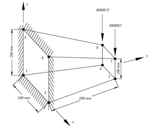
Finally, a parabolic voute corbel discretized with only a 20-node hexahedral finite element (H20) was statically analyzed. In Fig. 5, it is possible to verify the dimensions of the structure, points of application of the loads, crimped nodes, in addition to the numbering used for the nodes to carry out the discretization of the structure via the Finite Element Method.

Table 5 shows the displacements, in the most requested nodes, obtained by the present work in the z axis.

Table 5 – Corbel with parabolic voute - Nodal displacements in z

Nodes	MS250 (mm)	HS350 (mm)	SS304 (mm)	SI718 (mm)
1	0.00000	0.00000	0.00000	0.00000
3	0.00222	0.00222	0.00239	0.00222
15	-0.00191	-0.00191	-0.00195	-0.00184
16	-0.00392	-0.00392	-0.00413	-0.00385
18	-0.00148	-0.00148	-0.00158	-0.00147
20	0.00432	0.00432	0.00453	0.00424

Finally, Tab. 6 and Tab. 7 show the results obtained for the von Mises stresses and the elementary stresses, respectively.

Strain	MS250 (N/mm²)	HS350 (N/mm²)	SS304 (N/mm²)	SI718 (N/mm²)
${\textstyle {\sigma }_{\mbox{1}}}$	0.76680	0.76680	0.75990	0.76640
${\displaystyle {\sigma }_{\mbox{2}}}$	0.84610	0.84610	0.91860	0.89950
${\textstyle {\sigma }_{\mbox{3}}}$	2.49200	2.49200	2.59500	2.58600
${\textstyle {\sigma }_{\mbox{4}}}$	4.00300	4.00300	4.18400	4.15100
${\textstyle {\sigma }_{\mbox{5}}}$	2.94500	2.94500	2.84600	2.88800
${\textstyle {\sigma }_{\mbox{6}}}$	2.81200	2.81200	3.07700	3.01100
${\textstyle {\sigma }_{\mbox{7}}}$	13.99000	13.99000	15.30000	14.86000
${\textstyle {\sigma }_{\mbox{8}}}$	1.86800	1.86800	1.99200	1.96700

4. CONCLUSIONS

It is noteworthy that the computational program implemented for the 4-node tetrahedral 4 element, when demonstrated in example 1, presented the values ​​of the nodal displacements with a percentage difference of 0.00075% when compared with the values ​​found in the literature. As for the solids analyzed in this work, the lowest nodal displacement occurred for the superalloy inconel 718, with stainless steel having the highest nodal displacement.

For the examples in which the solids were solved with the 8-node and 20-node hexahedral finite elements, the integrals were solved numerically with the aid of the Gauss-Legendre Method (Gauss Quadrature). When analyzing the solids with the materials under study, it was found that for the analysis of nodal displacements, the superalloy inconel 718 obtained the lowest value of nodal displacement and stainless steel, in general, had the highest value. of displacement. In addition, it is added that in the case of structures with curvilinear geometries, H₂₀ would be the most recommended finite element to carry out the analysis.

For such analyses, it is possible to highlight how much the Modulus of Elasticity and the Poisson coefficient influence the resistance capacity of a solid when it is requested by a load, in addition to showing that the Modulus of Elasticity is inversely proportional to its deformability, thus showing that the greater the Modulus of Elasticity, the less the structure becomes deformed.

Since in the present research, for the analysis of stresses, the von Mises method was used for all examples, it is concluded that none of the analyzed materials came to fail, due to this, the fact that the stress values ​​of von Mises obtained did not exceed the yield stress values ​​of the analyzed materials.

It is concluded, therefore, that the developed implementation was satisfactory, contributing with precise values ​​of tension, deformation and displacement in solids subjected to a certain type of loading.

REFERENCES

[1] ZIENKIEWICZ, O. C., La Methods' des elements fínits (translated from the English), Pluralis, France, 1976.

[2] GALLAGHER, R. H., Introduction aux elements finis(translated from the English by J .L. Claudon), Pluralis, France, 1976.

[3] ABSI, E., Methode de calcul numérique en elaticité, Eyrolles, France, 1978.

[4] ROCKEY, K.C., Evans,H.R., Griffiths, D.W. and Nethercot, D.A., Elements finis, (translated from the English by C. Gomes), Eyrolles, France, 1979.

[5] IMBERT, J. F., Analyse des structures par elémentsfinis, Cepadues Ed., France, 1979.

[6] CHAPMAN, S. J., 2007, “Fortran 90/95 for Scientists and Engineers”, McGraw-Hill, 2nd ed.

[7] Chandrupatla, T.R., Belegundu, A.D., 2012, “Introduction to Finite Elements in Engineering”, 4rd ed. Pearson Education Limited, Edinburgh Gate, Reino Unido.