Revision as of 17:18, 15 December 2021 (view source) Crenan (talk | contribs) ← Older edit		Revision as of 15:23, 19 December 2021 (view source) Crenan (talk | contribs) Newer edit →
Line 2:		Line 2:
	==Fractal dimension measured over areas and perimeters using “Box Counting” technique applied over a Mandelbrot figure.label1==		==Fractal dimension measured over areas and perimeters using “Box Counting” technique applied over a Mandelbrot figure.label1==
−	'''C.  R.  Acosta1, F.  Peñuñuri 1, I. Pérez-Quintana 1'''	+	'''C.  R.  Acosta1, F.  Peñuñuri 1, O. Carvente 1'''
	-->		-->

---

Revision as of 15:23, 19 December 2021

Abstract

Measuring fractal dimension in general is made over edges of a figure, however this kind of calculations could be made over a 1D, 2D or even a 3D images. With the FracLac plugin of ImageJ application, it has been possible to measure both dimensions, over the area and over the edge of a Mandelbrot fractal, using the Box Counting technique.

keywords

Box Countig, Mandelbort fractal, Fractal dimension, ImageJ

Facultad de Ingeniería de la Universidad Autónoma de Yucatán

organization = Applied Physics Department, Facultad de Ingeniería de la Universidad Autónoma de Yucatán addressline = Av. Industrias no contaminates por anillo periférico norte S/N city = Mérida postcode = 97310 state = Yucatán country = Mexico

Research highlight 1 Research highlight 2

1 Introduction

Historical measurements with a straight line function over the England coast line made by Benoit Mandelbrot using different scales represented as “measuring rods” [1,2], which is based on a Lewis Fry Richardson's idea [3], can be calculated directly with any of the simplified data tables (1, 2), shown below.

Table. 1 The magnitude of scale is in kms.

Scale (s)	Long. (L)	Ln(s)	Ln(L)
200	2350	5.2983	7.7622
100	2775	4.6052	7.9284
50	3425	5.2983	8.1389

Table. 2 The scale is relative to the greatest magnitude.

Scale (s)	Long. (L)	Ln(s)	Ln(L)
200/200	2350	0.0000	7.7622
100/200	2775	-6.6931	7.9284
50/200	3425	-1.3863	8.1389

Linear regression calculations from data of the first table (1), are made directly over the scale, while in the second data table, greatest magnitude is used as reference (2).

Result of linear adjustment over data from any of both tables is the equation (1)

${\displaystyle f\left(x\right)=-0.27x+7.75}$

(1)

With an equation like shown (1) Mandelbrot identified the slope of as ${\textstyle m=1-D}$

${\displaystyle \ln \left[L\left(s\right)\right]=\left(1-D\right)\ln \left(s\right)+b}$

(2)

so the fractal dimension is ${\textstyle D=1.27}$

However there is another method to measure the same quantity and is knowing as “Box Counting Fractal” and is based on the idea of using “boxes” (squares) of the same size to fill the edge of entire figure and counting the number of boxes, then the longitude is given by ${\textstyle L\approx N\xi _{k}}$, where ${\textstyle \xi _{k}}$ is the size of one side o a box, change size of a generic box (${\textstyle \xi _{k}}$) and measure ${\textstyle L}$ again, doing this procedure by “practically” six or seven times, there are enough data to make a linear approximation [3]. But if an area is measured the relation is ${\textstyle A\approx N\xi _{k}^{2}}$ and if a volume is measured, the rule now is given by ${\textstyle V\approx N\xi _{k}^{3}}$, based on this ideas there is a power law for any dimension [2]:

${\displaystyle N\approx {\frac {L}{\xi _{k}}}\;\;{;}\;\;N\approx {\frac {A}{\xi _{k}^{2}}}\;\;{;}\;\;N\approx {\frac {V}{\xi _{k}^{3}}}\;\;\Rightarrow \;\;N\propto {\frac {1}{\xi _{k}^{D}}}}$

And by analogy with the fractal dimension, ${\textstyle D_{B}}$ that is generally called “capacity” or “box dimension” is defined by the relation (3) [4]

${\displaystyle D_{B}=\lim _{\xi _{k}\to 0}{\frac {\ln N\left(\xi _{k}\right)}{\ln \left({\frac {1}{\xi _{k}}}\right)}}\;\;\;\;{\hbox{if the limit exists.}}}$

(3)

If the box counting technique is utilized to calculate again the fractal dimension of the England coast line, table (3) must be used [5].

Table. 3 Data to calculate fractal dimension ${\displaystyle D_{B}}$ using “Box Counting” technique.

Scale (s)	Long. (L)	Ln(1/s)	Ln(L)
1	2350	0.0000	7.7622
0.5	5550	0.6931	8.6216
0.25	13700	1.3863	9.5252

The result of applying the linear adjustment over the data table (3) is the equation shown below (4).

${\displaystyle f\left(x\right)=1.27x+7.75}$

(4)

and it could be seen that the fractal dimension is given directly form the slope of the equation ${\textstyle D_{B}=1.27}$.

So there are two methods to calculate the fractal dimension, but if “measuring rods” are used, some additional operations must be made to obtain the result. In the “Box Counting Fractal” technique the result is directly the slope of straight line equation (4) [6].

2 ImageJ application

The “ImageJ” app is a free software from the project “SciJava OSS” used to images processing, with this powerful tool we can manipulate and measure any graphic file, and in conjunction with the FracLac plugin (that it is used to make calculations over fractals) we can obtain the fractal dimension based on the box counting (BC) method [6].

The direction to download “ImageJ” app is: https://imagej.nih.gov/ij/download.html

But must be selected the version that works with corresponding Operating System.

Install the app and use it to know the tool, but even when the software has a specific process to measure fractal dimension (Analyze-${\textstyle >}$Tools-${\textstyle >}$Fractal Box Counting), this is a limited characteristic of the app and we could use it as a first approach, in the sense that it didn't shows the boxes it draws and how changes in box's sizes are made.

The direction to download the “FracLac” plugin is: http://rsb.info.nih.gov/ij/plugins/fraclac/Frac_Lac.jar

To install the plugin go to Plugins-${\textstyle >}$Install, locate the folder where Frac_Lac.jar file was downloaded and select “open”. After the plugin is installed “ImageJ” program must be closed completely.

Open the program again, go to Plugins and must see the “Fractal Analysis” option as an additional sub-menu and “FracLac” as a sub-process.

Now, all the “ambience” is prepared to make ours first measurements. Then a graphic file in a png, jpg or bmp format must be opened, and so even when the calculations are made in pixels is preferable that the graphic have a printed scale.

2.1 Preliminary measurement

As a first step a scale must be established on the figure, so with this objective, open a graphic file and in the toolbar choose the “Straight” tool.

Figure 1: Toolbar of the ImageJ app.

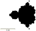
Over the Mandelbrot figure, locate the scale and with the shift button and the mouse pressed, touch one end of the scale and without release go to the other end, then release.

Figure 2: Mandelbrot figure with measure over the scale.

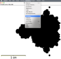
After this, go to menu and over “Analyze” select “Set Scale” put in the “Known distance” the value of the scale and in unit write the name of the scale.

Figure 3: Setting the scale of the figure.

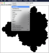
Calculations over the open figure can be made, but also another strategy can be taken, that is with “Rectangle” button of the toolbar choose an area, without the scale, that it is wanted to measure and on the menu select “Image” and the sub-process “Duplicate”, generates another figure with a different name proposed. So there are two figures and the original can be closed. With this new image active, select “Process” on the menu and go to “Binary” process, and “Make Binary” sub-process. Now if wants to calculate the fractal dimension of the figure's perimeter, must find the edges or can outline the graphic, at this step of the process the image is prepared to be measured.

Figure 4: Menu for finding the edges of the figure.

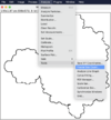
Then select “Analize” on the menu go to “Tools” process and “Fractal Box Counting” sub-process, this procedure gives a first result of the fractal dimension ${\textstyle D_{B}}$ as a result of the “Box Counting” technique, but this is just a preliminary measure, that is because the boxes can't be seen, just the result.

Figure 5: Menu for calculate directly the fractal dimension by the box counting method.

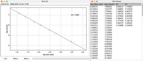
Figure 6: Result of calculations of fractal dimension over the Mandelbrot figure.

3 Using the FracLac plugin

In order to apply the “FracLac” plugin over any figure, the same treatment must be given as before, stablish the scale of the figure, that is to corroborate any measure is made,“Binarize” the picture and duplicate it and if wants to calculate fractal dimension of the perimeter, find the edges or outline the figure.

After figure was prepared, go to the “Plugins” section of the menu and in the “Fractal Analysis” process, accede to the sub-process of “FracLac”.

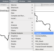
Figure 7: Menu to FracLac sub-process.

A new toolbar is open, from where the “BC” button that is located in the left superior corner must be choosen, a Pop Up appear that must be accepted and not include “Select for legacy mode”. A menu of characteristic appear and in “Grid design” puts number one, that is because grid must have just one origin, if wants more than one origin, then change this number. Modify the “Graphic options” as is shown on a red circle over the figure (8). Just make this changes if wants to measure fractal dimension of a perimeter line.

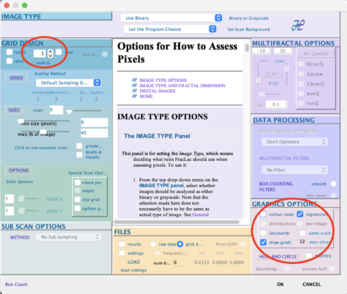
Figure 8: FracLac characteristics menu.

After given the characteristics of box counting, must press the“Scan” button (that is below the “Box Counting” button), then “FracLac” operate it's internal calculations and gives various results, two of them are shown, the image in tif format and the box counting data.

Figure 9: Two of the analysis results given by the plugin's operations.

The tif image gives 14 moments of the calculations over the perimeter, that could be extracted each one of them as an individual figure, four of them are shown in figure (10).

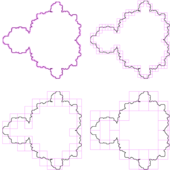
Figure 10: Four moments of the box counting calculations.

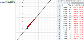
The calculation's data could be saved in csv format, that is compatible with apps, as Numbers, Excel, Mathematica etc. The fractal dimension is given in this file too, however if for some reason wants to make the linear regression adjustment, the columns two and three are the appropriate ones, as is shown in figure (11).

Then the process to calculate fractal dimension from a perimeter of any figure could be made in two ways; one is with an automatic operation of ImageJ (but we don't see any boxes), that gives a graph and a csv file. The box's size is defined by user and are between six to nine sizes. The other process is with the plugin “FracLac”, where all the steps of the process are shown even the boxes used in fourteen moments of calculations.

Results of the fractal dimension obtained in both procedures must gives values very close one to the other, not exactly the same, because the first one is made with 9 or less box's sizes, and the second one is made with 100 box's sizes.

Figure 11: Linear adjustment of columns two an three of data from file in csv format.

4 Fractal dimension of an image's area

Performing calculation of the ${\textstyle D_{B}}$ again, but now for the area of Mandelbrot's fractal figure, so let's do the whole procedure of opening the image, setting the scale, selecting the work area, duplicating the image, and finally “Binarize” the image, and an important part of the process is that we do not look for the edges or outline the image. Locates the “Plugins” tab, goes down to “Fractal Analysis” and the “FracLac” sub-process. The toolbar opens, in which it has to be given the initial parameters, select the “Box Counting” (BC) button, accept the “Pop Up” and do not include the inherited mode "Select for legacy mode".

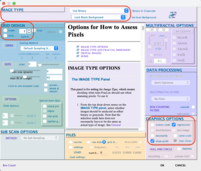
Now, since the DB of a figure's area are going to be measured, in the “Image Type” section, first line must have “Use binary” but in second line choose “Lock Black Background” if background is black,that is the one that wants to avoid, it means that measurement will be made over figure's white part. If wants to measure over figure's black part, then choose "Lock White Background", the other parameters are set as previously did.

Figure 12: BC menu's characteristic for measurement of ${\displaystyle D_{B}}$ over a figure's area.

Choose "Ok" at the bottom of BC menu's, and the "Pop Up" of "Show Regression Line Summaries" appears, which accept.

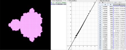
Once the characteristics of the measurements have been established select the "Scan" button, which is just below the "Box Counting" button. The "FracLac" plugin performs its internal procedures and gives us several results, but the box count is now done on the white area and the result of the fractal dimension is obtained, which is ${\textstyle D_{B}=1.7614}$.

Figure 13: Results of ${\displaystyle D_{B}}$ over a figure's area.

The data file is saved in csv format and the necessary calculations are made to fit a straight line with the data in columns 2 and 3, it must be taken into account that the natural logarithm of the reciprocal of the scale is plotted against the logarithm natural of the number of boxes, the equation of the straight line is: ${\textstyle y=1.76124x+0.31013}$ and the result of the fractal dimension is directly the slope, which is ${\textstyle D_{B}=1.76124}$.

5 Conclusions

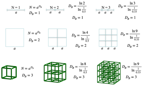
So there is the question, what does the fractal dimension measure? To answer it based on the “Box Counting” methodology, let's take a line of length ${\textstyle a}$, a square and a cube with sides also ${\textstyle a}$ and measure their fractal dimensions.

Figure 14: Calculation of fractal dimension ${\displaystyle D_{B}}$ over a line, a square and a cube.

Using the box counting technique it has been measured in this work the fractal dimension ${\textstyle D_{B}}$ of a Mandelbrot fractal figure with two different process [7,8,9].

• Measurement of the fractal dimension of the image perimeter.

• Measurement of the fractal dimension of the image area.

Both measurements of the fractal dimension are different and both means how far they are from the corresponding Euclidean dimension [10,11].

BIBLIOGRAPHY

[1] B. Mandelbrot, “The fractal geometry of nature”, W. H. Freeman 1982. [2] B. Mandelbrot, “Self-affine and Fractal dimension”, Physica Scripta, vol. 32(4), 1985, pp. 257-260. [3] B. Mandelbrot, “How Long Is the Coast of Britain? Statistical Self-Similarity and Fractional Dimension”, Science, 156(3775), pp. 636-638, DOI: 10.1126/science.156.3775.636 [4] D. Gatzouras and S. Lalley, “Hausdorff and box dimensions of certainself-affine fractals”, Indiana University Mathematics Journal, vol. 41(2), 1992, pp. 533-568. [5] A. Husain, J. Reddy, D. Bisht and M. Sajid “Fractal dimension of coastline of Australia”, Nature Scientific Report, 2021, doi.org/10.1038/s41598-021-85405-0 [6] C. Schneider, W. Rasband and K. Eliceiri “NIH Image to ImageJ: 25 years of image analysis”, Nature Methods 9, 2012, pp. 671–675. [7] P. Shanmugavadivu and V. Sivakumar, “Fractal dimension-bound spatiotemporal analysis of digital mammograms”, The European Physics Journal Special Topics, vol. 225, pp. 137-146. [8] B. Bárány, M. Hochman and A. Rapaport, “Hausdorff dimension of planar self-affine measures”, Inventiones Mathematicae. vol. 16, 2019, pp. 601–659. [9] H. Christensen, and O. Driver, “The fractal nature of clouds in global storm-resolving models”, ArXiv:2108.08565v1, 19 Aug 2021. [10] H. Strogatz, ``Nonlinear Dynamics and Chaos: With applications to Physics, Biology, Chemistry and Engineering, Westview Press, Boulder CO. USA, 2nd edition (2015).

[11] R. Devaney “A first course in chaotic dynamical systems theory and experiment” CRC Press, Florida USA, 2nd edition (2020).