CarolinaHN5 (talk | contribs) (Tag: Visual edit) |
CarolinaHN5 (talk | contribs) (Tag: Visual edit) |
||
| Line 1,068: | Line 1,068: | ||
<div id="_Hlk56241762" class="center" style="width: auto; margin-left: auto; margin-right: auto;"> | <div id="_Hlk56241762" class="center" style="width: auto; margin-left: auto; margin-right: auto;"> | ||
| − | [[ | + | [[File:Review 995707923686-image7.png|600x600px]] </div> |
<div class="center" style="width: auto; margin-left: auto; margin-right: auto;"> | <div class="center" style="width: auto; margin-left: auto; margin-right: auto;"> | ||
Revision as of 16:06, 31 May 2022
ABSTRACT
When cranial bone needs to be removed or lost, subsequent reconstruction of the defect is necessary to protect the underlying brain, correct aesthetic deformities, or both. Cranioplasty surgical procedures are performed to correct the skull defects requiring reconstruction of form and function. Personalized cranial implants can repair severe injuries to the skull can be done through This study presents the optimization of cranial titanium implants. A total of sixty different models were subjected to a simulation by Finite Element Analysis (FEA) applying the mechanical properties of a grade 5 titanium alloy (Ti6Al4V) implant material. The material was subjected to intracranial pressure (ICP) conditions, with a typical range (10 mm Hg) and twelve fixation points in the boundary conditions. An artificial neural network (ANN) was created to connect the designs, obtaining maximum displacements. Optimal designs were obtained using a generalized reduced gradient that minimizes the amount of material, maintaining as a restriction a maximum displacement of 0.1 mm for the 5th to 95th percentiles, which represent the group of individuals under study.
Keywords: Cranial implant; Artificial neural network (ANN); Generalized reduced gradient method (GRG); Optimization; Titanium alloy (Ti6Al4V); Finite Element Analysis (FEA)
1. Introduction
The human head is often subjected to impact during automobile accidents, falls, or sport-related events. These impact conditions can lead to mechanically induced head injury, which constitutes one of the major causes of accidental death [1]. Head injuries could be grouped into three categories: scalp damage, skull fracture, brain injury, or a combination of these [2,3].
Improving indications for cranial decompressive procedures, mainly after traumatic injuries and vascular lesions had led to a demand for effective bone substitutes in cranial reconstruction, particularly in large and complex bone defects. Cranioplasty is carried out to restore the morphological and functional anatomy of the cranial vault, to protect the brain, thus avoiding neurological disorders, deficits, or changes in the cerebrospinal fluid, and to restore cranial aesthetics [4,5]. Cranioplasty surgery does not only offer cosmetic and sometimes lifesaving benefits but also gives relief to psychological drawbacks and improves the life quality for patients [6]. Cranioplasty surgical procedures may be conducted by using autografting (the implant is taken from the patient's body) and allografting (implant taken from a donor’s body) or alloplastic (non-biologic such as polymeric and metallic) materials [7].
Metallic alloplastic materials, used in alloys with titanium, have mechanical properties greater than bone, manufacturing ease, and good resistance to corrosion degradation [8]. Besides, due to good mechanical properties superior to those of human bone, such as modulus of elasticity and yield strength, they lend themselves to load-bearing applications in the human body and prevent fractures after use.
Ti-containing alloys, such as the commonly used surgical Grade 5 titanium (Ti6Al4V), present low density, a high strength-to-weight ratio, high biocompatibility, and form an oxide layer to which bone progenitor cells can strongly adhere [9]. Titanium is used in the cranium for fixation devices such as plates and screws, mesh, or solid plates, and in combination with other materials such as inert plastic or ceramic components [10].
The selection of cranial implants must satisfy several important criteria, such as biocompatibility, customized geometry to ensure direct contact with bone tissue, and sufficient mechanical properties to withstand function related stress [11]. Technical readiness for clinical application, short lead time, low cost, and ease of manufacture for alloplastic cranioplasty are also important considerations [12].
On the other hand, developments in tissue engineering are moving forward, exploiting advanced designs and fabrication technologies to design and produce implants, patterns or templates that enable the fabrication of custom-made prostheses without requiring a model of the anatomy to be made [13]. In this regard, the optimization of implants becomes relevant to reduce the weight, material usage, and cost of the implants while assuring their structural integrity and functionality [14], at the same time, parameters of the material such as porosity can be adjusted [15].
Particularly, the skull provides the structure to the head and face while protecting the brain, it is composed of flat and irregular bones. The skull can be divided into a facial part called Viscerocranium, the bones which form the face, and a Neurocranium, known as the braincase, that protects the brain and brainstem [16,17].
The presence of a lesion (intra- or extra-axial) can generate displacement of the brain's midline, causing herniation, compression of basal cisterns, increased intracranial pressure, and leading to death. A midline shift greater than 0.5 cm is a predictor of a bad result in the neurological outcome of patients with head injuries hospitalized in intensive care [18].
It is essential to classify the injury to address the diagnostic study of a seriously ill patient due to severe head trauma. The most widespread and defended of the classifications of traumatic brain injury (TBI) by CT is that of Marshall et al. [19], which is based on the state of the mesencephalic cisterns, the degree of deviation from the midline, and the presence or absence of focal lesion (Lesions diffuse-type I, II, III or IV).
Modern design and manufacturing engineering technologies have greatly improved how modern craniofacial implants are designed and fabricated. However, sophisticated optimization algorithms that simultaneously deal with multi-functional designs on multiple length scales need to be developed [14].
Artificial neural networks (ANN) models are successfully used in different fields of study; after they are satisfactorily competent and tested, it can generalize rules and respond rapidly (instantaneously) to input data to predict required outputs within the domains covered by the training examples. Moreover, it can handle many data sets, implicitly detect the complex nonlinear relationships between dependent and independent variables, and detect all possible interactions between predictor variables [20,21]. The multi-layer perceptron (MLP) network, typically referred to as back propagation (BP) network, is the most popular ANN in engineering issues and may have one or several hidden layers.
The optimization is to obtain the best possible result in a process or system by determining the values of the variables that intervene; in mathematical terms, it consists of searching for a minimum or maximum of a function. For example, the design of bone implants allows the design of structures to meet the desired objectives and restrictions [22,23]. The generalized reduced gradient or GRG search method is a nonlinear constraint optimization method used in the Excel Solver [24].
Implementing computer-aided design (CAD) and optimization in implant design is hampered by the high computational cost; however, the application of neural networks can solve the problem by reducing simulation times. In addition, the integration of optimization technology with simulation and artificial intelligence techniques will reduce experimental times and costs.
This study aims to determine the optimal design that minimizes the amount of Ti6Al4V material, subject to a maximum displacement constraint of 0.1 mm (total analysis deformation), for a neurocranial implant. The rest of the paper is organized in materials and methods, where it is presented from data acquisition, implant design, functional finite element analysis, and artificial neural network. Subsequently, a results section presents a normality test, implant design, functional analysis, predictive neural network, GRG optimization, and finally, the conclusions.
The challenge of this article is to determine the savings obtained by minimizing the volume of material and the cost savings by reducing the design time of the implant, concerning other methodologies recorded in specialized literature. To overcome it, a future investigation is recommended where the cost factor is measured.
2. Materials and methods
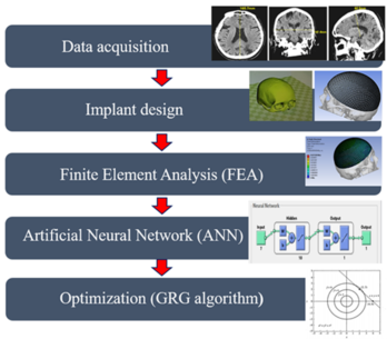
The proposed methodology for the design and optimization of titanium cranial implants is shown in the block diagram in Figure 1. The whole methodology is divided into five modules: data acquisition, implant design, finite element analysis (FEA), artificial neural network (ANN), and optimization (GRG method).
2.1. Data acquisition (Cranial anatomy approach)
In the present study, six variables were selected using anatomical points, and a craniometric study was performed (130 Mexican adult skulls with ages between 18 and 50 years were analyzed). The participants of the study come from fourteen different states (Chihuahua, Guerrero, Sinaloa, Sonora, Tijuana, Hidalgo, Jalisco, Mexico City, Guanajuato, Colima, Coahuila, Queretaro, and Veracruz). The inclusion criteria were free of physical injuries, without cranial fracture, deformities, or surgeries in the skull.
An anthropometer brand Rosscraft model Campell® 10 RC-10 with 18 cm range, a Rosscraft metallic ribbon for anthropometric use with 200 cm range, each equipment has an accuracy of 0.5 mm; and an ErgoMeasure vertical anthropometer with 500 cm range and precision of ±1mm; were used to measure the anthropometric dimensions.
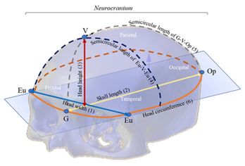
The anthropometric dimensions used in the study indicate the distance between two referenced craniometric points: Glabella (G), Vertex (V), Opisthocranion (Op), and Eurion (Eu). Figure 2 shows an overview of the skull bones of the Neurocranium (Frontal, Parietal, Temporal and Occipital bones) and the variables (craniometric dimensions) used in the study with craniometric reference landmarks: Eu-Eu = head width (1), G-Op = skull length (2), V-G = head height (3), Eu-V-Eu = Semicircular length of Eu-V-Eu (4), G-V-Op = Semicircular length G-V-Op (5) and head circumference (6).
Following the ethics committee of the Autonomous University of Ciudad Juárez (UACJ), the protocol applied was reviewed and approved. The participants signed a consent form accepting their participation in the study and the absence of health risks when participating in the study. The information collected was treated confidentially and was used only for academic purposes. A team of 3 anthropometrics was trained to perform cranial anthropometric measurements. Descriptive statistics (mean, standard deviation, minimum, maximum, range, and 5th, 25th, 50th, 75th, and 95th percentiles) were calculated. The Kolmogorov-Smirnov test was applied to ensure the normality of the data, considering a significance value of 0.05. All statistical procedures were conducted using SPSSv17 software.
2.2. Implant design
The design of the implant must satisfy two main requirements: geometry and functionality [25-27]. The functionality considers the geometry, dimensions, and materials to satisfy functional requirements such as structural performance. From the values obtained in the craniometric study, the values corresponding to the 5th, 25th, 50th, 75th, and 95th percentiles were selected. The bone implants were designed using SolidWorks software, applying the values obtained.
Different designs were performed for each percentile varying the thickness of the implant between 0.5 mm to 1 mm, thickness commonly applied in commercial meshes, the size (diameter of 3 mm, 4 mm, 5 mm, and 6 mm), and separation of the holes (5 ° and 10 °) in such a way that, for each percentile, there is a different geometry and volume. The percentage of empty spaces (A) was calculated using Equation 1, where the total volume corresponds to the geometry without the holes and the final volume with holes. The volume values were determined using the software, while the models were exported in Parasolid format (*.x_t).
(1)
The specifications of hole size, separation of holes and thickness of each design corresponding to 5th, 25th, 50th, 75th, and 95th percentiles are shown in Table 1.
| Table 1. Implants design specifications. | |||||||||||||
| Specifications of design | 1 | 2 | 3 | 4 | 5 | 6 | 7 | 8 | 9 | 10 | 11 | 12 | Percentile |
| Hole diameter (mm) | 3 | 3 | 3 | 3 | 4 | 4 | 4 | 4 | 5 | 5 | 6 | 6 | 5th |
| Separation of holes (degrees) | 5 | 5 | 10 | 10 | 5 | 5 | 10 | 10 | 10 | 10 | 10 | 10 | |
| Thickness (mm) | 0.5 | 1 | 0.5 | 1 | 0.5 | 1 | 0.5 | 1 | 0.5 | 1 | 0.5 | 1 | |
| Specifications of design | 13 | 14 | 15 | 16 | 17 | 18 | 19 | 20 | 21 | 22 | 23 | 24 | Percentile |
| Hole diameter (mm) | 3 | 3 | 3 | 3 | 4 | 4 | 4 | 4 | 5 | 5 | 6 | 6 | 25th |
| Separation of holes (degrees) | 5 | 5 | 10 | 10 | 5 | 5 | 10 | 10 | 10 | 10 | 10 | 10 | |
| Thickness (mm) | 0.5 | 1 | 0.5 | 1 | 0.5 | 1 | 0.5 | 1 | 0.5 | 1 | 0.5 | 1 | |
| Specifications of design | 25 | 26 | 27 | 28 | 29 | 30 | 31 | 32 | 33 | 34 | 35 | 36 | Percentile |
| Hole diameter (mm) | 3 | 3 | 3 | 3 | 4 | 4 | 4 | 4 | 5 | 5 | 6 | 6 | 50th |
| Separation of holes (degrees) | 5 | 5 | 10 | 10 | 5 | 5 | 10 | 10 | 10 | 10 | 10 | 10 | |
| Thickness (mm) | 0.5 | 1 | 0.5 | 1 | 0.5 | 1 | 0.5 | 1 | 0.5 | 1 | 0.5 | 1 | |
| Specifications of design | 37 | 38 | 39 | 40 | 41 | 42 | 43 | 44 | 45 | 46 | 47 | 48 | Percentile |
| Hole diameter (mm) | 3 | 3 | 3 | 3 | 4 | 4 | 4 | 4 | 5 | 5 | 6 | 6 | 75th |
| Separation of holes (degrees) | 5 | 5 | 10 | 10 | 5 | 5 | 10 | 10 | 10 | 10 | 10 | 10 | |
| Thickness (mm) | 0.5 | 1 | 0.5 | 1 | 0.5 | 1 | 0.5 | 1 | 0.5 | 1 | 0.5 | 1 | |
| Specifications of design | 49 | 50 | 51 | 52 | 53 | 54 | 55 | 56 | 57 | 58 | 59 | 60 | Percentile |
| Hole diameter (mm) | 3 | 3 | 3 | 3 | 4 | 4 | 4 | 4 | 5 | 5 | 6 | 6 | 95th |
| Separation of holes (degrees) | 5 | 5 | 10 | 10 | 5 | 5 | 10 | 10 | 10 | 10 | 10 | 10 | |
| Thickness (mm) | 0.5 | 1 | 0.5 | 1 | 0.5 | 1 | 0.5 | 1 | 0.5 | 1 | 0.5 | 1 | |
2.3. Normality test
Table 2 shows the normality test results, conducted using the Kolmogorov-Smirnov test. Due to the p-value of the six variables being higher than 0.05, data is considered normal, and it is possible to perform additional statistics and model analysis.
| Table 2. Normality Test Results. | ||
| Skull dimension | Kolmogorov Smirnov value | P-value |
| Eu-Eu | 0.462 | 0.983 |
| G-Op | 0.938 | 0.342 |
| Head Circumference G-Op | 0.650 | 0.791 |
| G-V-Op | 0.771 | 0.591 |
| Eu-V-Eu | 0.703 | 0.707 |
| V-G | 0.898 | 0.395 |
2.4. Data acquisition and implant design
Table 3 shows the descriptive statistics of craniometrics dimensions (mean, the standard deviation, the minimum, the maximum, and the 5th, 25th, 50th, 75th, and 95th percentiles) of head width (Eu-Eu), skull length (G-Op), head height (V-G), Eu-V-Eu Semicircular length, G-V-Op Semicircular length, and head circumference.
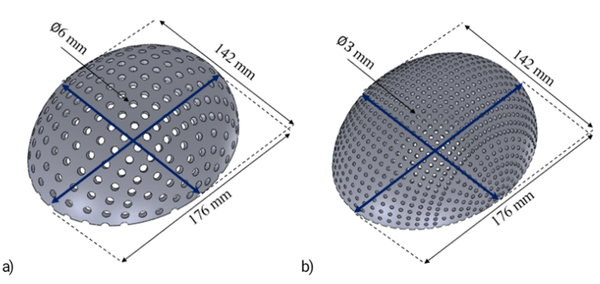
According to the percentiles values shown in Table 3, a total of sixty tridimensional implants were designed using SolidWorks software. Figure 3 shows two 3D designs of the skull implant, corresponding to the dimensions of the 5th percentile with variations in their geometry. The percentage of empty spaces (A) and the volume of each design are shown in Table 4.
| Table 3. Craniometrics dimensions descriptive statistics. | |||||||
| Descriptive statistics | Head width
Eu-Eu (mm) |
Cranial length
G-Op (mm) |
Head Circumference
(mm) |
G-V-Op Semicircular length (mm) | Head height V-G
(mm) |
Eu-V-Eu Semicircular length
(mm) | |
| Mean ± SD | 153.50 ± 6.71 | 190.40 ± 9.28 | 563.73±20.02 | 313.28 ± 29.50
|
76.57 ± 3.29
|
311.57 ± 19.51 | |
| Minimum | 138.70 | 171.00 | 508.00 | 261.00 | 69.70 | 263.30 | |
| Maximum | 170.00 | 218.70 | 614.00 | 525.00 | 86.60 | 370.00 | |
| Percentiles | 5 | 142.40 | 176.00 | 529.60 | 274.70 | 71.50 | 277.90 |
| 25 | 148.60 | 183.70 | 551.30 | 297.70 | 74.20 | 297.90 | |
| 50 | 153.50 | 190.00 | 563.20 | 312.50 | 76.40 | 313.80 | |
| 75 | 157.80 | 195.70 | 577.70 | 325.80 | 78.50 | 325.00 | |
| 95 | 165.70 | 209.30 | 600.00 | 353.10 | 83.30 | 343.40 | |
| Table 4. Implant designs’ percentage of empty spaces (A) and the volume. | |||||||||||||
| Specifications of design | 1 | 2 | 3 | 4 | 5 | 6 | 7 | 8 | 9 | 10 | 11 | 12 | Percentile |
| Empty spaces (%) | 17.12 | 18.38 | 4 | 5.21 | 31.88 | 33.21 | 7.17 | 8.41 | 11.35 | 12.6 | 16.62 | 17.88 | 5th |
| Volume (mm3) | 15104 | 29968 | 17521 | 34807 | 12621 | 25000 | 16918 | 33595 | 16142 | 32043 | 15193 | 30145 | |
| Specifications of design | 13 | 14 | 15 | 16 | 17 | 18 | 19 | 20 | 21 | 22 | 23 | 24 | Percentile |
| Empty spaces (%) | 15.88 | 15.97 | 3.71 | 3.73 | 29.52 | 29.68 | 6.66 | 6.69 | 10.54 | 10.6 | 15.42 | 15.5 | 25th |
| Volume (mm3) | 16813 | 33374 | 19229 | 38207 | 14330 | 28408 | 18626 | 37004 | 17850 | 35448 | 16901 | 33551 | |
| Specifications of design | 25 | 26 | 27 | 28 | 29 | 30 | 31 | 32 | 33 | 34 | 35 | 36 | Percentile |
| Empty spaces (%) | 20.73 | 16.73 | 9.98 | 11.53 | 24.2 | 18.22 | 12.43 | 12.8 | 15.09 | 14.11 | 18.01 | 15.49 | 50th |
| Volume (mm3) | 18178 | 36096 | 20595 | 40930 | 15695 | 31129 | 19991 | 39723 | 19215 | 38170 | 18266 | 36273 | |
| Specifications of design | 37 | 38 | 39 | 40 | 41 | 42 | 43 | 44 | 45 | 46 | 47 | 48 | Percentile |
| Empty spaces (%) | 18.5 | 15.72 | 8.39 | 10.68 | 21.75 | 17.17 | 10.7 | 11.91 | 13.21 | 13.19 | 15.95 | 15.03 | 75th |
| Volume (mm3) | 19516 | 38588 | 20465 | 43422 | 16944 | 33620 | 21241 | 42215 | 21845 | 40662 | 19428 | 38764 | |
| Specifications of design | 49 | 50 | 51 | 52 | 53 | 54 | 55 | 56 | 57 | 58 | 59 | 60 | Percentile |
| Empty spaces (%) | 15.11 | 3.51 | 3.53 | 27.89 | 28.04 | 6.31 | 6.34 | 9.98 | 10.03 | 14.59 | 14.67 | 14.52 | 95th |
| Volume (mm3) | 22092 | 43902 | 24518 | 48746 | 19604 | 38924 | 23909 | 47536 | 23132 | 45981 | 22181 | 44079 | |
2.5. Functionality analysis (Finite element analysis)
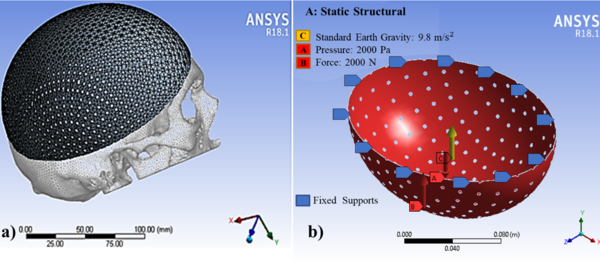
Sixty models were transferred to the ANSYS Workbench 18.1 (ANSYS Inc) to generate the FEA models. The FEA mesh of the computational model (Figure 4a) consisted of 10 nodes tetrahedral and 20 nodes hexahedral elements (Ansys non-linear elements). The minimum element size of the mesh was 0.5 mm for all models. Element sizes were chosen based on preliminary tests and sensitivity calculations. Subsequently, quality controls of the elements were carried out.
The use of titanium material (Ti6Al4V) was simulated. Table 5 shows the mechanical properties of this material [28].
| Table 5. Ti6Al4V Mechanical properties. | |
| Property | Value |
| Yield strength (σy) | 896 MPa |
| Ultimate yield strength (σu) | 965 MPa |
| Elastic modulus (E) | 116 GPa |
| Poisson ratio | 0.34 |
According to Nahum et al. [29] and Schneider et al. [30], minimum thresholds of 2450 N for men and 2000 N for women were suggested for clinically significant skull fractures. Messerer [31] determined that approximately 2000 N were needed to fracture the subcondylar region. In this study, a uniform distributed force of 2000 N was applied in the Y-axis in all the simulated designs located in the craniometric vertex (V), in the upper part of the implant, as seen in Figure 4b.
The static pressure of 10 mm Hg was considered based on intracranial pressure conditions [32] and a standard earth gravity of 9.8 m/s2; the pressure was applied on the inner surface and evenly distributed over an implant area. As Wen et al. [33], the bone-implant contact area was assumed to be complete osseous integration, and so the contact area was simulated by using a surface-to-surface option fully bonded. Both loading and boundary conditions of the FEA models are shown in Figure 4b.
Figure 4. A model with a) tetrahedral and hexahedral mesh with b) fixation point and forces.
The screws to hold the implant are not simulated since these are considered independent elements of the implant. Although the screws interact with the model after surgery, their design is independent of the model proposed in this article; therefore, the structural integrity of the cranial implant is not affected during the design.
The mechanical properties of implants were all treated as isotropic, homogeneous, and linear elastic. Therefore, the safety factor is high in all the proposed designs, and large deformations are not considered since the element is expected to deflect (maximum displacement of 0.1 mm), but without exceeding the yield point, the element does not reach the plastic failure.
Because the present work focused on optimizing the geometry, the mechanical performance of the bone-implant construction was analyzed only in terms of the deformation parameter. According to Didier et al., [34], no study considers the phenomenon of “protection against stress” between the bone and the implant in its optimization process. Therefore, in this work, the optimization approach only considers the mechanical characteristics of the optimized part.
2.6. Artificial neural network application
An artificial neural network (ANN) based on multi-layer perceptron (MPL-ANN) was elaborated with the MATLAB Neural Network Toolbox to process the obtained data and create a predictive system that relates the anthropometric dimensions, the volume, and the thickness with the maximum displacement of the cranial implants designs. The MLP-ANN model predicted the maximum displacement; Figure 5 shows the final architecture of the MPL-ANN proposed. It consisted of three layers: an input, a hidden, and an output layer. Each layer consists of a few neurons and connections; weights were established between neurons. In the input layer, seven variables were introduced: thickness specifications, hole size, separation of holes, volume, head width, cranial length, and head height; the output layer was the maximum displacement of the designs. Randomly 70% of the data obtained in the simulation were used as training data, 15% as a validation, and the remaining 15% as a test. The performance and accuracy of the MLP model were examined by measuring the determination coefficient (R2). Then, the values of the 30th, 40th, 60th and 80th percentiles were introduced to obtain the maximum displacement of their corresponding designs without submitting to simulation.
New theoretical designs were proposed for the 30th, 40th, 60th and 80th percentiles, which were not subjected to simulation; however, the maximum displacement was obtained for each of them using the artificial neural network created previously. This information was subsequently used for optimization.
2.7. Generalized reduced gradient optimization
The optimal point in a function corresponds to the value of x where the derivative is equal to zero. Furthermore, the second derivative indicates whether the optimum is a minimum or a maximum. If (negative), it is a maximum; if (positive), it is a minimum. In a two-dimensional function the directional derivative can be calculated from the partial derivatives along the x and y axes by, as shown Equation 2:
(2)
Where partial derivatives are evaluated at x = a and y = b. The gradient (Equation 3) is a vector that is related to the directional derivative of at the point x = a and y = b.
(3)
The generalized gradient to n dimensions (Equation 4) is defined in vector notation as:
(4)
Both the first and second derivatives offer valuable information in the search for the optimum. The first derivative provides a maximum tilt path for the function and indicates when the optimum has been reached. Once in the optimum, the second derivative will indicate if it is a maximum (negative) or if it is a minimum (positive). The determinant of a matrix formed with the second derivatives is known as the Hessian (H) of :
(5)
Equation 5 is the Hessian of , in addition to providing a means of discriminating whether a multidimensional function has reached the optimum, allows searches that include second-order curvature. The GRG method requires the storage of an approximation of the Hessian matrix (equation 5) and performs a search varying the displacement amplitude for the improvement of the reduced objective. The Excel solver is based on the GRG method, and they are evolutionary algorithms according to the input data and the objective function. First, a search direction is established to improve the objective function using a quasi-Newton procedure (BFGS), which requires the storage of an approximation of the Hessian matrix. Once the search direction is established, a one-dimensional search is performed using a variable step size procedure. The tool considers several points in the search space [35].
Using simple linear regression using the least squares method in Minitab statistical software, a multivariate linear regression model was obtained using four design variables (skull length, thickness, diameter, and hole spacing) as continuous predictors and final volume implant as a response variable as follows (Equation 6):
(6)
where:
V = Response variable (Volume).
Xi = Independent variables or predictors.
β0 = Intersection coefficient.
βi = Linear coefficient.
εi = Random experimental error.
Subsequently, using the Curve Fitting Toolbox of MATLAB, a polynomial function was found that best fits the data of the predictor variables length of the skull and the maximum displacement obtained by FEM with the final volume of the implant (response variable). The terms were identified as significant for selecting the models, and the highest adjusted R2 value with a significance level of p <0.05.
The optimal designs for each percentile that minimizes the Ti6Al4V material were found using a GRG method in an Excel solver, maintaining a maximum displacement of 0.1 mm as a restriction, since in this condition, a diffuse type II lesion may occur. The mesencephalic cisterns are present in diffuse-type II lesions, and the midline moderately deviates equal to or less than 5 mm [19]. The optimal designs were obtained by optimization equations where the minimum volume was used as the objective, using the maximum displacement (less than or equal to 0.1 mm) as the restriction. We optimized nine new theoretical designs for the 5th, 25th, 30th, 40th, 50th, 60th, 75th, 80th, and 95th percentiles and then validated them with MEF.
To solve the disadvantage of the generalized reduced gradient search method for finding the local minimum, the value of the step length was varied, and it was observed whether there was an improvement in the objective function. A search was performed with a different value if no improvement was observed. In the same way, the method can take us to a saddle point if the Hessian matrix is not positively defined. As all the identified eigenvalues of the Hessian matrix were positive, it can be determined that our function is being approximated by a quadratic function of circular or ellipsoidal contours that have a minimum.
3. Results
3.1. Functionality analysis and predictive neural network
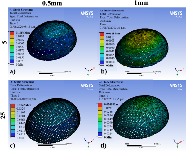
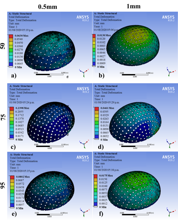
The geometric models were subjected to the simulation by FEM in the ANSYS® software. Table 5 shows the results of the 60 simulations with an applied force of 2000N, where the displacements obtained corresponding to different designs are observed for the 5th, 25th, 50th, 75th, and 95th percentiles: at thicknesses of 0.5 and 1 mm. Figures 6 and 7 show the results of 10 of the 60 simulations; it could be noticed that displacements are greater for 0.5 mm than those established for 1 mm. The 75th percentile for 0.5 mm thickness shows the highest value, and the other percentiles observed are within the range of the maximum allowed offset. According to Figures 6 and 7, these displacements are observed mainly at the diametric base of each percentile studied.
| Table 5. Implant designs’ maximum displacement. | |||||||||||||
| Design | 1 | 2 | 3 | 4 | 5 | 6 | 7 | 8 | 9 | 10 | 11 | 12 | Percentile |
| Maximum displacement (mm) | 0.161 | 0.034 | 0.105 | 0.011 | 0.117 | 0.027 | 0.084 | 0.008 | 0.086 | 0.017 | 0.092 | 0.027 | 5th |
| Design | 13 | 14 | 15 | 16 | 17 | 18 | 19 | 20 | 21 | 22 | 23 | 24 | Percentile |
| Maximum displacement (mm) | 0.154 | 0.034 | 0.071 | 0.013 | 0.154 | 0.030 | 0.066 | 0.013 | 0.073 | 0.018 | 0.087 | 0.024 | 25th |
| Design | 25 | 26 | 27 | 28 | 29 | 30 | 31 | 32 | 33 | 34 | 35 | 36 | Percentile |
| Maximum displacement (mm) | 0.211 | 0.038 | 0.060 | 0.013 | 0,157 | 0.029 | 0.063 | 0.013 | 0.073 | 0.015 | 0.103 | 0.023 | 50th |
| Design | 37 | 38 | 39 | 40 | 41 | 42 | 43 | 44 | 45 | 46 | 47 | 48 | Percentile |
| Maximum displacement (mm) | 0.207 | 0.039 | 0.061 | 0.013 | 0.134 | 0.019 | 0.065 | 0.012 | 0.095 | 0.020 | 0.239 | 0.046 | 75h |
| Design | 49 | 50 | 51 | 52 | 53 | 54 | 55 | 56 | 57 | 58 | 59 | 60 | Percentile |
| Maximum displacement (mm) | 0.183 | 0.035 | 0.075 | 0.011 | 0.092 | 0.006 | 0.070 | 0.015 | 0.080 | 0.017 | 0.092 | 0.019 | 95h |
To predict the mechanical behavior of the new designs (maximum displacements) of cranial implants, an MLP-ANN was elaborated to relate the created designs' specifications (thickness, hole size, separation of holes, volume, head width, cranial length, and head height).
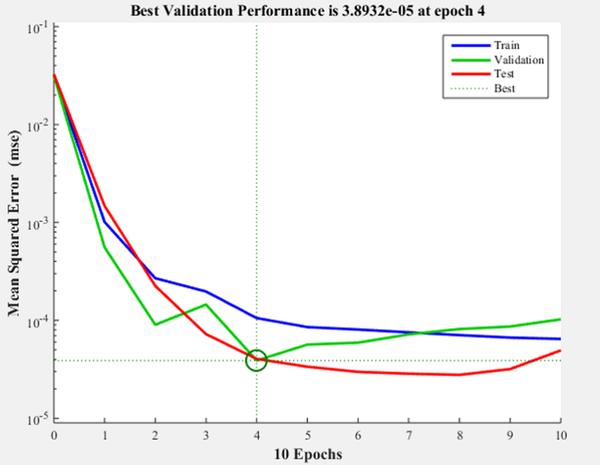
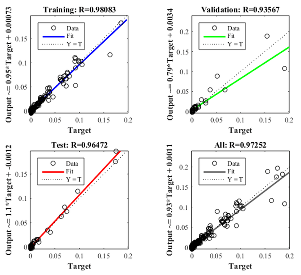
Figure 8 shows the iteration in which the validation performance reached a minimum. The epoch is the number of times the algorithm was executed; in this case, the best validation performance was at epoch 4. As a result, the validation and test curves are remarkably similar; therefore, there is no excess of adjustment. Figure 9 shows the neural network selected based on its regression graph, where a global R2 value of 0.9725 was obtained, showing a 97% relationship between the outputs of the network and the targets.
The ANN obtained was used to predict the maximum displacement of new theoretical designs of craniofacial implants for the 30th, 40th, 60th, and 80th percentile.
3.2. Optimization
Using simple linear regression utilizing the Minitab statistical software, a linear model was obtained, applying the design variables as continuous predictors (skull length, thickness, diameter, and hole spacing) and the final implant volume as a response. The terms were identified as significant for selecting the model using the R2 and general statistics of the significant F test. Table 6 shows the analysis of variance and the results of the DF (Degree of Freedom), SS Fit (Sum of Squares), MS Fit (Mean Square), the F value, and the P-value of the variables analyzed. The degrees of freedom indicate the number of independent elements in the sum of squares for each component of the model; having 60 different designs, we obtain a total of 59 DF, and the sum of squares (SS) is the deviation of the mean of the factor level estimated around the general mean. The Mean Square (MS) is an unbiased estimator of the variance and is the sum of squares divided by the degrees of freedom. According to the values obtained in the F and P values, it was observed that each of the terms is statistically significant when obtaining p values <0.05 and higher Fisher's F values with a significance level alpha = 0.05. A mathematical model was developed to relate the design variables to the final volume of the implant, obtaining an R2 of 0.97. Table 7 shows an adjusted R2 of 97.31%, indicating that the model can estimate the volume using the design variables as predictors.
| Table 6. Variance analysis. | ||||||
| Source | DF | SS Adjust | MS Adjust | F-value | P-value | |
| Regression | 4 | 6211342822 | 1552835705 | 534.30 | 0.000 | |
| Skull Length (G-Op) | 1 | 754802731 | 754802731 | 259.71 | 0.000 | |
| Thickness | 1 | 5156845417 | 5156845417 | 1774.38 | 0.000 | |
| Diameter | 1 | 100376598 | 100376598 | 34.54 | 0.000 | |
| Separation | 1 | 292120699 | 292120699 | 100.51 | 0.000 | |
| Error | 55 | 159845539 | 2906283 | |||
| Total | 59 | 6371188360 | ||||
| Table 7. Model Summary. | |||
| Standard error | R-square | R-squared (adjusted) |
R-squared (predicted) |
| 1704.78 | 97.49% | 97.31% | 96.94% |
The relation between the variables skull length (x1), thickness (x2), diameter (x3), and hole spacing (x4) to the final implant volume (V) is presented in Equation 7.
(7)
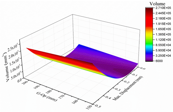
Using the anthropometric dimensions of the skull and modifying the design variables (thickness and percentage of empty spaces), a mathematical model was found in Matlab using the MATLAB Curve Fitting application (Figure 10), obtaining an R2 of 0.97. Equation 8 relates the length of the skull (x1), the maximum displacement (y1), and the volume (V) is as follows:
(8)
The resulting equations were entered as formulas in a spreadsheet in Excel. First, a cell was selected for each decision variable: the design variables thickness, diameter, and hole spacing. Then, a cell was created for the objective function, which corresponds to the final volume of the implant.
Finally, the optimal designs for each percentile were found using the solver tool, which minimizes the amount of material (Ti6Al4V) while maintaining a maximum displacement of 0.1 mm. The optimal designs are shown in Table 8 and were obtained with the minimum volume by equation 7 as the objective, using the maximum displacement of equation 8 as a restriction (minor or equal to 0.1 mm). The maximum displacement of these designs was validated using MEF and shown in Table 8.
| Table 8. Values corresponding to the optimal designs of cranial implants. | |||||||
| Percentile | x1
Skull length (mm) |
x2
Thickness (mm) |
x3
Diameter (mm) |
x4
Separation (°) |
V
Volume (mm3) |
MEF Maximum displacement (mm) | |
| 5 | 176.00 | 0.56 | 4.77 | 5.18 | 12333.68 | 0.0843 | |
| 25 | 183.70 | 0.55 | 4.80 | 5.15 | 14137.10 | 0.0906 | |
| 30 | 185.00 | 0.55 | 4.81 | 5.15 | 14440.00 | 0.0934 | |
| 40 | 188.00 | 0.54 | 4.75 | 5.19 | 15139.00 | 0.0969 | |
| 50 | 190.00 | 0.53 | 4.76 | 5.18 | 15605.00 | 0.0991 | |
| 60 | 193.18 | 0.52 | 4.70 | 5.24 | 16345.94 | 0.0997 | |
| 75 | 195.70 | 0.52 | 4.71 | 5.23 | 16933.10 | 0.0989 | |
| 80 | 196.00 | 0.52 | 4.72 | 5.23 | 17003.00 | 0.0974 | |
| 95 | 209.30 | 0.50 | 4.74 | 5.20 | 18666.62 | 0.0912 | |
4. Discussion
Nowadays, designing a 3D cranial implant model is a challenge. Some cranial implant models designed with Ti6Al4V and other polymeric materials have been proposed by other authors [36,37]. Morais et al. [38] proposed a Deep Learning (DL) approach toward automated CAD for the design of cranial implants. On the other hand, Stutz et al. [39] proposed machine learning-based approaches to shape completion. Wu et al. [40] proposed an architecture called 3D Shape Nets, in which the input shapes are given as input to a convolutional Deep Belief network that learns a probabilistic distribution from 3D volumes for 3D reconstruction. However, this type of network is difficult to train. For this study, the optimization of Ti6Al4V cranial implants was achieved by applying a novel proposal based on three tools, the generalized reduced gradient (GRG) search method, artificial neural networks (ANN), and applying the finite element method (FEM). According to work presented by Şensoy et al. [41], to optimize topologies for mandibular distractor plates and the geometry design, they used MATLAB-PYTHON-ANSYS and found superior stability with a less implant volume.
Ameen et al. [42] found an optimally designed implant with 0.5 mm thickness from test loading. In our case, optimal designs were found for the 5th to 95th percentiles, which minimizes the amount of Ti6Al4V material while maintaining a maximum offset of 0.1 mm, which is compatible with a large part of individuals of productive age of the Mexican population since they were considered in the data collection stage, individuals from 18 to 50 years of age, representative of 14 states of the Mexican Republic.
The optimization was based on the mechanical analysis (maximum displacement) of the design under the FEM simulation using normal intracranial pressure conditions (ICP = 10 mm Hg), twelve fixation points, and a force of 2000 N to lighten the structure (minimize volume) while maintaining the mechanical functionality and protection provided by the implant.
5. Conclusions
For this study, the optimization of Ti6Al4V cranial implants was achieved by applying a novel proposal based on three tools, the generalized reduced gradient (GRG) search method, artificial neural networks (ANN), and applying the finite element method (FEM). As a result, optimal designs were found for the 5th to 95th percentiles, which minimizes the amount of Ti6Al4V material while maintaining a maximum offset of 0.1 mm, which is compatible with a large part of individuals of productive age of the Mexican population since they were considered in the data collection stage, individuals from 18 to 50 years of age, representative of 14 states of the Mexican Republic.
The optimization was based on the mechanical analysis (maximum displacement) of the design under the FEM simulation using normal intracranial pressure conditions (ICP = 10 mm Hg), twelve fixation points, and a force of 2000 N to lighten the structure (minimize volume) while maintaining the mechanical functionality and protection provided by the implant.
Using an ANN, it was possible to predict the response for numerous combinations of geometric parameters without creating or modifying new models by significantly reducing design and simulation time. The GRG optimization allowed us to identify the most efficient and lightweight conceptual designs, finding the geometries of the 3D models that require less volume of material for their manufacture, considerably reducing the final cost of the implant.
Future research proposes applying the same methodology and comparing different biocompatible materials; for example, in addition to Ti6Al4V, consider steel and polymethyl methacrylate, including the variable cost of the material. A second future investigation includes other software that facilitates the design stage, such as Easycranea, Easyimplant, MIMICS, Biobuild, MeVisLab, BioCAD, or 3D-Doctor. Also include other artificial intelligence tools such as simulated annealing metaheuristics, genetic algorithms, and taboo search to find the best solutions that reduce the volume of material and, consequently, the cost.
A third investigation that is proposed is to compare the monetary savings obtained by applying the methodology proposed in this work with other registered in specialized literature.
ACKNOWLEDGEMENTS
M.I. Martínez-Valencia and J.L. Díaz León want to thank the Mexican National Council for Science and Technology (CONACyT) for undertaking their master's and doctoral's degree, respectively, with the scholarship numbers 474489 and 473353. The first author wants to thank CONACyT and Educafin-SUBE for the scholarship to carry out a research stay at the Autonomous University of Ciudad Juárez. The authors want to acknowledge the Centro Médico Quirúrgico (CMQ) hospital for its support with cranial computed tomography (CT) data. Finally, the authors want to thank R. Lesso Arroyo (RIP) for encouraging them to continue with biomechanical and biomedical research.
REFERENCES
- [1] Sahoo D., Deck C., Yoganandan N., Willinger R. Development of Skull Fracture Criterion Based on Real-World Head Trauma Simulations Using Finite Element Head Model. Journal of the Mechanical Behavior of Biomedical Materials, 57:24-41, 2016. DOI: https://doi.org/10.1016/j.jmbbm.2015.11.014.
- [2] Bešenski N. Traumatic injuries: imaging of head injuries. European Radiology, 12(6):1237–1252, 2002. DOI: https://doi.org/10.1007/s00330-002-1355-9.
- [3] Li G., Wang F., Otte D., Simms C. Characteristics of pedestrian head injuries observed from real world collision data. Accident analysis and prevention, 129:362-366, 2019. DOI: https://doi.org/10.1016/j.aap.2019.05.007.
- [4] Shah A.M., Jung H., Skirboll S. Materials used in cranioplasty: a history and analysis. Neurosurgical Focus, 36(4):E19, 2014. DOI: https://doi.org/10.3171/2014.2.FOCUS13561.
- [5] Bogu, V.P., Kumar, Y.R., Khanara, A.K. Modelling and structural analysis of skull/cranial implant: beyond mid-line deformities. Acta of Bioengineering and Biomechanics, 19(1):125-131, 2017. DOI: 10.5277/ABB-00547-2016-04.
- [6] Aydin S., Kucukyuruk B., Abuzayed B., Aydin S., Sanus G.Z. Cranioplasty: review of materials and techniques. Journal of Neurosciences in Rural Practice, 2(2):162, 2011. DOI: 10.4103/0976-3147.83584.
- [7] Lu B., Ou H., Shi S.Q., Long H., Chen J. Titanium based cranial reconstruction using incremental sheet forming. International Journal of Material Forming, 9(3):361-370, 2016. DOI: https://doi.org/10.1007/s12289-014-1205-8.
- [8] Jardini A.L., Larosa M.A., Maciel Filho R., et al. Cranial reconstruction: 3D biomodel and custom-built implant created using additive manufacturing. Journal of Cranio-Maxillofacial Surgery, 42(8):1877-1884, 2014. DOI: https://doi.org/10.1016/j.jcms.2014.07.006.
- [9] Andani M.T., Moghaddam N.S., Haberland C., Dean D., Miller M.J., Elahinia M. Metals for bone implants. Part 1. Powder metallurgy and implant rendering. Acta Biomaterialia, 10(10):4058-4070, 2014. DOI: https://doi.org/10.1016/j.actbio.2014.06.025.
- [10] Durham S.R., McComb J.G., Levy M.L. Correction of Large (>25 cm2) Cranial Defects with Reinforced” Hydroxyapatite Cement: Technique and Complications. Neurosurgery, 52(4):842-845, 2003. DOI: https://doi.org/10.1227/01.NEU.0000054220.01290.8E.
- [11] Tsouknidas A., Maropoulos S., Savvakis S., Michailidis N. FEM assisted evaluation of PMMA and Ti6Al4V as materials for cranioplasty resulting mechanical behaviour and the neurocranial protection. Bio-Medical Materials and Engineering, 21(3):139-147, 2011. DOI: DOI: 10.3233/BME-2011-0663.
- [12] Spetzger U., Vougioukas V., Schipper J. Materials and techniques for osseous skull reconstruction. Minimally Invasive Therapy and Allied Technologies, 19(2):110-121, 2010. DOI: https://doi.org/10.3109/13645701003644087.
- [13] Bibb R., Eggbeer D., Evans P., Bocca A., Sugar A. Rapid manufacture of custom‐fitting surgical guides. Rapid Prototyping Journal, 15(5):346-354, 2009. DOI: https://doi.org/10.1108/13552540910993879.
- [14] Wang X., Xu S., Zhou S., et al. Topological design and additive manufacturing of porous metals for bone scaffolds and orthopedic implants: A review. Biomaterials, 83:127–141, 2016. DOI: https://doi.org/10.1016/j.biomaterials.2016.01.012.
- [15] Parthasarathy J., Starly B., Raman S., Christensen A. Mechanical evaluation of porous titanium (Ti6Al4V) structures with electron beam melting (EBM). Journal of the Mechanical Behavior of Biomedical Materials, 3(3):249-259, 2010. DOI: https://doi.org/10.1016/j.jmbbm.2009.10.006.
- [16] Lieberman D. The evolution of the human head. Harvard University Press, London, 2011.
- [17] Singh V. Textbook of Anatomy Head, Neck, and Brain (Vol. 3). Elsevier Health Sciences, New Delhi, 2014.
- [18] Sartori P., Alvarado L., Chirveches M., Urrutia M., Yampolsky B. Mediciones frecuentes en el sistema nervioso central mediante tomografía computada e imágenes de resonancia magnética. Revista Argentina de Radiología/Argentinian Journal of Radiology, 84(01):009-016, 2020.
- [19] Marshall L.F. Head injury: recent past, present, and future. Neurosurgery, 47(3): 546-561, 2000.
- [20] Pattanayak S., Loha C., Hauchhum L., Sailo L. Application of MLP-ANN models for estimating the higher heating value of bamboo biomass. Biomass Conversion Biorefinery,1-10, 2020. DOI: https://doi.org/10.1007/s13399-020-00685-2.
- [21] Kalantary S., Jahani S., Pourbabaki R., Beigzadeh Z. Application of ANN modeling techniques in the prediction of the diameter of PCL/gelatin nanofibers in environmental and medical studies. The Royal Society of Chemistry Advances, 9(43):24858-24874, 2019. DOI: 10.1039/C9RA04927D.
- [22] Allaire G. Shape Optimization by the Homogenization Method. Springer Science & Business Media, New York, 2012.
- [23] Bendsoe M., Sigmund O. Topology Optimization. Theory, Methods, and Applications. Springer Science & Business Media, Berlin, 2013.
- [24] Smith S., Lasdon L. Solving large sparse nonlinear programs using GRG. ORSA Journal on Computing, 4(1):2-15, 1992. DOI: https://doi.org/10.1287/ijoc.4.1.2.
- [25] Unterhofer C., Wipplinger C., Verius M., Recheis W., Thomé C., Ortler M. Reconstruction of large cranial defects with poly-methyl-methacrylate (PMMA) using a rapid prototyping model and a new technique for intraoperative implant modeling. Polish Journal of Neurology and Neurosurgery, 51(3):214-220, 2017. DOI: https://doi.org/10.1016/j.pjnns.2017.02.007.
- [26] Xiaojun C., Lu X., Xing L., Jan E. Computer-aided implant design for the restoration of cranial defects. Scientific Reports, 7:4199-4200, 2017. DOI: https://doi.org/10.1038/s41598-017-04454-6.
- [27] Yashwant K.M., Sidharth S. Design and additive manufacturing of patient‑specific cranial and pelvic bone implants from computed tomography data. ournal of the Brazilian Society of Mechanical Sciences and Engineering, 40:503-513, 2018. DOI: https://doi.org/10.1007/s40430-018-1425-9.
- [28] Ratner B., Hoffman A., Schoen F., Lemons J. Biomaterials Science. An Introduction to Materials in Medicine 3rd ed. Elsevier Science, San Diego, California, 2012.
- [29] Nahum A., Gatts J., Gadd C., Danforth J. Impact tolerance of the skull and face. (No. 680785). SAE Technical Paper, 1968. DOI: https://doi.org/10.4271/680785.
- [30] Schneider D.C., Nahum A.M. Impact studies of facial bones and skull. (No. 720965). SAE Technical Paper. 1972. DOI: https://doi.org/10.4271/720965
- [31] Messerer O. Über Elasticität und Festigkeit der menschlichen Knochen. Cotta, 1880.
- [32] Nagasao T., Miyamoto J., Jiang H., Kaneko T., Tamaki T. Biomechanical Analysis of the Effect of Intracranial Pressure on the Orbital Distances in Trigonocephaly. Cleft Palate-Craniofacial Journal, 48(2):190-196, 2011. DOI: https://doi.org/10.1597/09-027.
- [33] Wen H., Guo W., Liang R., et al. Finite element analysis of three zygomatic implant techniques for the severely atrophic edentulous maxilla. Journal of Prosthetic Dentistry, 111(3):203–215, 2014. DOI: https://doi.org/10.1016/j.prosdent.2013.05.004.
- [34] Didier P., Piotrowski B., Le Coz G., Laheurte P. Topology optimization for the control of load transfer at the bone-implant interface: a preliminary numerical study. Computer Methods in Biomechanics and Biomedical Engineering, 23(sup1):S82-S84, 2020. DOI: https://doi.org/10.1080/10255842.2020.1812167.
- [35] Hashemi S.H., Dehghani S.A.M., Samimi S.E., Dinmohammad M., Hashemi S.A. Performance comparison of GRG algorithm with evolutionary algorithms in an aqueous electrolyte system. odeling Earth Systems and Environment, 6:2103–2110, 2020. DOI: https://doi.org/10.1007/s40808-020-00818-6.
- [36] Marcián P., Narra N., Borák L., Chamrad J., Wolff J. Biomechanical performance of cranial implants with different thicknesses and material properties: A finite element study. Computers in Biology and Medicine, 109:43-52, 2019. DOI: https://doi.org/10.1016/j.compbiomed.2019.04.016
- [37] Moiduddin K., Darwish S., Al-Ahmari A., ElWatidy S., Mohammad A., Ameena W. Structural and mechanical characterization of custom design cranial implant created using additive manufacturing. Electronic Journal of Biotechnology, 29:22-31, 2017. DOI: https://doi.org/10.1016/j.ejbt.2017.06.005.
- [38] Morais A., Egger J., Alves V. Automated Computer-aided Design of Cranial Implants Using a Deep Volumetric Convolutional Denoising Autoencoder. In: Rocha Á, Adeli H, Reis L, Costanzo S, editors. WorldCIST'19 2019. Advances in Intelligent Systems and Computing; April 16-19. Springer, Cham, Galicia, Spain, 2019; 151-160. DOI: https://doi.org/10.1007/978-3-030-16187-3_15.
- [39] Stutz D., Geiger A. Learning 3D shape completion from laser scan data with weak supervision. Paper presented at: CVPR 2018. Proceedings of the IEEE Conference on Computer Vision and Pattern Recognition, 1955-1964, 2018.
- [40] Wu Z., Song S., Khosla A., et al. 3d shapenets: A deep representation for volumetric shapes. In Proceedings of the IEEE conference on computer vision and pattern recognition, 1912-1920, 2015.
- [41] Şensoy A.T., Kaymaz I., Ertaş Ü. Development of particle swarm and topology optimization-based modeling for mandibular distractor plates. Swarm and Evolutionary Computation, 53:100645, 2020. DOI: https://doi.org/10.1016/j.swevo.2020.100645.
- [42] Ameen W., Al‐Ahmari A., Mohammed M.K., Abdulhameed O., Umer U., Moiduddin K. Design, finite element analysis (FEA), and fabrication of custom titanium alloy cranial implant using electron beam melting additive manufacturing. Advances in Production Engineering & Management, 13(3):267-278, 2018. DOI: https://doi.org/10.14743/apem2018.3.289.
Document information
Published on 22/06/22
Accepted on 14/06/22
Submitted on 23/12/21
Volume 38, Issue 2, 2022
DOI: 10.23967/j.rimni.2022.06.004
Licence: CC BY-NC-SA license
Share this document
Keywords
claim authorship
Are you one of the authors of this document?
