m (Cinmemj moved page Draft Samper 249832658 to Coll et al 2014b) |
|||
| (24 intermediate revisions by 2 users not shown) | |||
| Line 1: | Line 1: | ||
| − | ==Robust volume mesh generation for non-watertight geometries== | + | <!-- metadata commented in wiki content |
| + | ==PhD Thesis Robust volume mesh generation for non-watertight geometries== | ||
| − | ''' | + | '''Abel Coll Sans |
| − | + | Supervisors: Pooyan Dadvand | |
| − | + | ||
| + | Eugenio Oñate Ibáñez de Navarra ''' | ||
''A mi padre.'' | ''A mi padre.'' | ||
| − | + | =Agradecimientos= | |
Con estas líneas quiero agradecer a todos aquellos que, de alguna manera, han contribuido a la realización de este trabajo. | Con estas líneas quiero agradecer a todos aquellos que, de alguna manera, han contribuido a la realización de este trabajo. | ||
| Line 31: | Line 32: | ||
A todos ellos, muchas gracias. | A todos ellos, muchas gracias. | ||
| + | top=3cm,bottom=1cm | ||
| + | --> | ||
| − | + | =Abstract= | |
Nowadays large part of the time needed to perform a numerical simulation is spent in preprocessing, especially in the geometry cleaning operations and mesh generation. Furthermore, these operations are not easy to automatize because they depend strongly on each geometrical model and they often need human interaction. Many of these operations are needed to obtain a watertight geometry. Even with a clean geometry, classical unstructured meshing methods (like Delaunay or Advancing Front based ones) present critical weak points like the need of a given quality in the boundary mesh or a relatively smooth size transition. These aspects decrease their robustness and imply an extra effort in order to reach the final mesh. Octree based meshers try to relax some of these requirements. | Nowadays large part of the time needed to perform a numerical simulation is spent in preprocessing, especially in the geometry cleaning operations and mesh generation. Furthermore, these operations are not easy to automatize because they depend strongly on each geometrical model and they often need human interaction. Many of these operations are needed to obtain a watertight geometry. Even with a clean geometry, classical unstructured meshing methods (like Delaunay or Advancing Front based ones) present critical weak points like the need of a given quality in the boundary mesh or a relatively smooth size transition. These aspects decrease their robustness and imply an extra effort in order to reach the final mesh. Octree based meshers try to relax some of these requirements. | ||
| Line 44: | Line 47: | ||
A shared memory parallel implementation of the algorithm has been done. The effectiveness of the algorithm and its implementation has been verified by some validation examples. | A shared memory parallel implementation of the algorithm has been done. The effectiveness of the algorithm and its implementation has been verified by some validation examples. | ||
| − | + | =Resum= | |
| − | + | ||
En l'actualitat gran part del temps emprat per córrer una simulació numerica esta dedicat al preprocés, especialment a les operacions de neteja de geometria i generació de malla. A més, aquestes operacions no són facils d'automatitzar degut a la seva forta dependencia del model geometric i sovint necessiten d'interacció humana. Moltes d'aquestes operacions són necessaries per aconseguir una definició topologicament hermetica de la geometria. Inclús amb una geometria neta, els metodes classics de mallat (com els basats en Delaunay o avancament frontal) presenten punts febles crítics com la necessitat d'una certa qualitat de les malles de contorn o una transició de mides relativament suau. Aquests aspectes disminueixen la seva robustesa i impliquen un esforc extra a l'hora d'obtenir la malla final. Els metodes de mallat basats en estructures ''octree'' relaxen alguns d'aquests requeriments. | En l'actualitat gran part del temps emprat per córrer una simulació numerica esta dedicat al preprocés, especialment a les operacions de neteja de geometria i generació de malla. A més, aquestes operacions no són facils d'automatitzar degut a la seva forta dependencia del model geometric i sovint necessiten d'interacció humana. Moltes d'aquestes operacions són necessaries per aconseguir una definició topologicament hermetica de la geometria. Inclús amb una geometria neta, els metodes classics de mallat (com els basats en Delaunay o avancament frontal) presenten punts febles crítics com la necessitat d'una certa qualitat de les malles de contorn o una transició de mides relativament suau. Aquests aspectes disminueixen la seva robustesa i impliquen un esforc extra a l'hora d'obtenir la malla final. Els metodes de mallat basats en estructures ''octree'' relaxen alguns d'aquests requeriments. | ||
| Line 57: | Line 59: | ||
S'ha dut a terme una implementació paral<math display="inline">\cdot </math>lela amb memoria compartida de l'algorisme. L'efectivitat del mateix i la seva implementació ha estat verificada mitjancant exemples de validació. | S'ha dut a terme una implementació paral<math display="inline">\cdot </math>lela amb memoria compartida de l'algorisme. L'efectivitat del mateix i la seva implementació ha estat verificada mitjancant exemples de validació. | ||
| − | = | + | =1 Introduction= |
| − | + | ||
| − | + | ||
Numerical simulations try to reproduce virtually a physical behavior by solving given equations in a specific domain. They are nowadays essential to understand some complex physical problems in scientific and engineering field. Although experimental setups can be build to study the specific behavior of a given phenomena, sometimes it is hard for these experiments (or even impossible depending on the scale of the tackled problem) to represent it accurately. The increasing advances in terms of computer science technology allow to treat larger and larger problems virtually (in the computer), so each time more and more numerical methods have been developed in the scientific field in order to capture the physics of complex problems. | Numerical simulations try to reproduce virtually a physical behavior by solving given equations in a specific domain. They are nowadays essential to understand some complex physical problems in scientific and engineering field. Although experimental setups can be build to study the specific behavior of a given phenomena, sometimes it is hard for these experiments (or even impossible depending on the scale of the tackled problem) to represent it accurately. The increasing advances in terms of computer science technology allow to treat larger and larger problems virtually (in the computer), so each time more and more numerical methods have been developed in the scientific field in order to capture the physics of complex problems. | ||
| Line 104: | Line 104: | ||
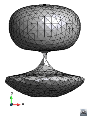
<div id='img-1'></div> | <div id='img-1'></div> | ||
| − | {| style="text-align: center; border: 1px solid #BBB; margin: 1em auto; width: | + | {| class="floating_imageSCP" style="text-align: center; border: 1px solid #BBB; margin: 1em auto; width: 100%;max-width: 100%;" |
|- | |- | ||
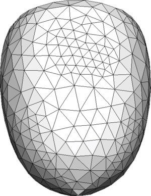
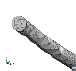
| − | |[[Image:draft_Samper_249832658-stl_input_boundary.png| | + | |[[Image:draft_Samper_249832658-monograph-stl_input_boundary.png|270px|Example of a 3D input boundary (represented with a mesh) where the quality of the triangles is very bad.]] |
|- style="text-align: center; font-size: 75%;" | |- style="text-align: center; font-size: 75%;" | ||
| colspan="1" | '''Figure 1:''' Example of a 3D input boundary (represented with a mesh) where the quality of the triangles is very bad. | | colspan="1" | '''Figure 1:''' Example of a 3D input boundary (represented with a mesh) where the quality of the triangles is very bad. | ||
| Line 150: | Line 150: | ||
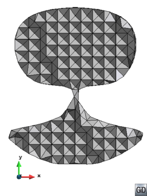
<div id='img-2'></div> | <div id='img-2'></div> | ||
| − | {| style="text-align: center; border: 1px solid #BBB; margin: 1em auto; width: | + | {| class="floating_imageSCP" style="text-align: center; border: 1px solid #BBB; margin: 1em auto; width: 100%;max-width: 100%;" |
|- | |- | ||
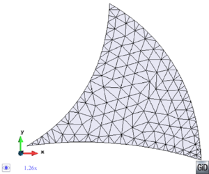
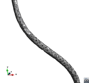
| − | |[[Image:draft_Samper_249832658-non_watertight_2D.png| | + | |[[Image:draft_Samper_249832658-monograph-non_watertight_2D.png|270px|Example of a 2D non watertight input boundary with gaps and overlapping entities.]] |
|- style="text-align: center; font-size: 75%;" | |- style="text-align: center; font-size: 75%;" | ||
| colspan="1" | '''Figure 2:''' Example of a 2D non watertight input boundary with gaps and overlapping entities. | | colspan="1" | '''Figure 2:''' Example of a 2D non watertight input boundary with gaps and overlapping entities. | ||
|} | |} | ||
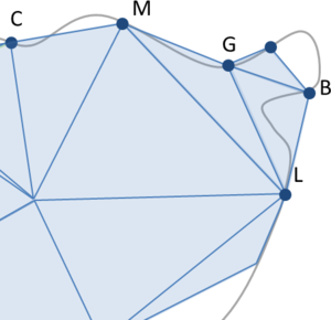
| − | ''Accept input data in geometry and mesh format''. The natural input for a mesher is the geometrical definition of the contours of the model. This geometrical definition can be represented in several ways, but the most common ones are CAD or mesh entities. In this document, when talking about CAD entities, the NURBS surfaces and curves <span id='citeF-4'></span>[[#cite-4|[4]]] (trimmed or not) will be considered, as they are the most general mathematical representation able to represent all the geometrical shapes. | + | * ''Accept input data in geometry and mesh format''. The natural input for a mesher is the geometrical definition of the contours of the model. This geometrical definition can be represented in several ways, but the most common ones are CAD or mesh entities. In this document, when talking about CAD entities, the NURBS surfaces and curves <span id='citeF-4'></span>[[#cite-4|[4]]] (trimmed or not) will be considered, as they are the most general mathematical representation able to represent all the geometrical shapes. |
Although the mesher should generate a mesh from a non-cleaned input geometry, some minimum criteria concerning topology or shape definition may be needed. | Although the mesher should generate a mesh from a non-cleaned input geometry, some minimum criteria concerning topology or shape definition may be needed. | ||
| Line 164: | Line 164: | ||
<div id='img-3'></div> | <div id='img-3'></div> | ||
| − | {| style="text-align: center; border: 1px solid #BBB; margin: 1em auto; width: | + | {| class="floating_imageSCP" style="text-align: center; border: 1px solid #BBB; margin: 1em auto; width: 100%;max-width: 100%;" |
|- | |- | ||
| − | |[[Image:draft_Samper_249832658-chordal_error.png| | + | |[[Image:draft_Samper_249832658-monograph-chordal_error.png|270px|Graphical representation of the chordal error in a 2D case. The black thick line represents the smooth geometry, and the gray thin line represents its mesh. The distance d is the chordal error of the element e]] |
|- style="text-align: center; font-size: 75%;" | |- style="text-align: center; font-size: 75%;" | ||
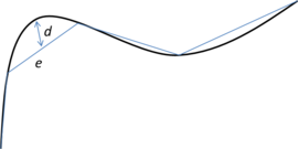
| colspan="1" | '''Figure 3:''' Graphical representation of the chordal error in a 2D case. The black thick line represents the smooth geometry, and the gray thin line represents its mesh. The distance <math>d</math> is the chordal error of the element <math>e</math> | | colspan="1" | '''Figure 3:''' Graphical representation of the chordal error in a 2D case. The black thick line represents the smooth geometry, and the gray thin line represents its mesh. The distance <math>d</math> is the chordal error of the element <math>e</math> | ||
| Line 184: | Line 184: | ||
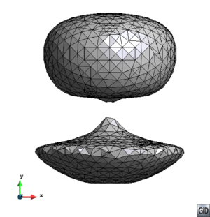
<div id='img-4'></div> | <div id='img-4'></div> | ||
| − | {| style="text-align: center; border: 1px solid #BBB; margin: 1em auto; width: 100%;max-width: 100%;" | + | {| class="floating_imageSCP" style="text-align: center; border: 1px solid #BBB; margin: 1em auto; width: 100%;max-width: 100%;" |
|- | |- | ||
| − | | | + | | |
| − | | | + | {| style="text-align: center; margin: 1em auto;min-width:50%;width:100%;" |
|- | |- | ||
| − | | | + | | [[Image:draft_Samper_249832658-monograph-volume_topology_geom.png|300px|Figures/chapter_introduction/volume_topology_geom]] |
| + | | [[Image:draft_Samper_249832658-monograph-volume_topology_mesh.png|300px|Figures/chapter_introduction/volume_topology_mesh]] | ||
| + | | [[Image:draft_Samper_249832658-monograph-volume_topology_mesh_2.png|300px|Figures/chapter_introduction/volume_topology_mesh_2]] | ||
| + | |- | ||
| + | | (a) | ||
| + | | (b) | ||
| + | | (c) | ||
| + | |||
| + | |} | ||
| + | |||
| + | |- | ||
| + | |||
|- style="text-align: center; font-size: 75%;" | |- style="text-align: center; font-size: 75%;" | ||
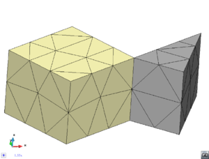
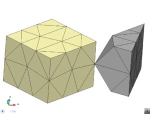
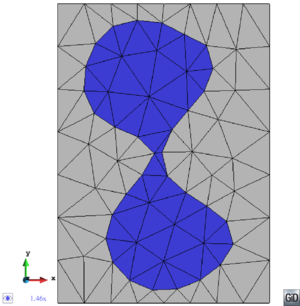
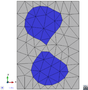
| − | | colspan=" | + | | colspan="1" | '''Figure 4:''' Topology preservation between two volumes and their meshes. '''(a)''' Two volumes in contact sharing a line. '''(b)''' Meshes of the volumes shown in (a) sharing the line elements corresponding to the mesh of the line shared by both volumes: the topology is preserved. '''(c)''' Meshes of the volumes shown in (a) not sharing line elements: the topology of the original model is not preserved. |
|} | |} | ||
| Line 197: | Line 208: | ||
<div id='img-5'></div> | <div id='img-5'></div> | ||
| − | {| style="text-align: center; border: 1px solid #BBB; margin: 1em auto; width: 100%;max-width: 100%;" | + | {| class="floating_imageSCP" style="text-align: center; border: 1px solid #BBB; margin: 1em auto; width: 100%;max-width: 100%;" |
|- | |- | ||
| − | | | + | | |
| − | | | + | {| style="text-align: center; margin: 1em auto;min-width:50%;width:100%;" |
|- | |- | ||
| − | | | + | | [[Image:draft_Samper_249832658-monograph-thin_part_geom.png|300px|Figures/chapter_introduction/thin_part_geom]] |
| + | | [[Image:draft_Samper_249832658-monograph-thin_part_mesh_1.png|300px|Figures/chapter_introduction/thin_part_mesh_1]] | ||
| + | | [[Image:draft_Samper_249832658-monograph-thin_part_mesh_2.png|300px|Figures/chapter_introduction/thin_part_mesh_2]] | ||
| + | |- | ||
| + | | (a) | ||
| + | | (b) | ||
| + | | (c) | ||
| + | |||
| + | |} | ||
| + | |||
| + | |- | ||
| + | |||
|- style="text-align: center; font-size: 75%;" | |- style="text-align: center; font-size: 75%;" | ||
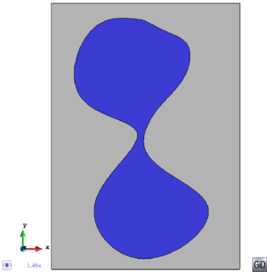
| − | | colspan=" | + | | colspan="1" | '''Figure 5:''' Example of surface mesh preserving or not the topology of the initial domain. '''(a)''' 2D geometrical domain formed by two surfaces (colored as blue and gray). '''(b)''' Mesh of the surfaces preserving the topology of the initial domain. '''(c)''' Mesh of the surfaces not preserving the topology of the initial domain. |
|} | |} | ||
| Line 212: | Line 234: | ||
<div id='img-6'></div> | <div id='img-6'></div> | ||
| − | {| style="text-align: center; border: 1px solid #BBB; margin: 1em auto; width: 100%;max-width: 100%;" | + | {| class="floating_imageSCP" style="text-align: center; border: 1px solid #BBB; margin: 1em auto; width: 100%;max-width: 100%;" |
|- | |- | ||
| − | | | + | | |
| − | | | + | {| style="text-align: center; margin: 1em auto;min-width:50%;width:100%;" |
|- | |- | ||
| − | | | + | | [[Image:draft_Samper_249832658-monograph-constrained_1.png|300px|Figures/chapter_introduction/constrained_1]] |
| + | | [[Image:draft_Samper_249832658-monograph-constrained_2.png|300px|Figures/chapter_introduction/constrained_2]] | ||
| + | | [[Image:draft_Samper_249832658-monograph-constrained_3.png|300px|Figures/chapter_introduction/constrained_3]] | ||
| + | |- | ||
| + | | (a) | ||
| + | | (b) | ||
| + | | (c) | ||
| + | |||
| + | |} | ||
| + | |||
| + | |- | ||
| + | |||
|- style="text-align: center; font-size: 75%;" | |- style="text-align: center; font-size: 75%;" | ||
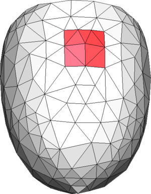
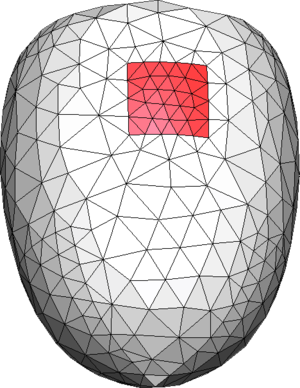
| − | | colspan=" | + | | colspan="1" | '''Figure 6:''' '''(a)''' Contour mesh of a volume with a set of triangles highlighted in red representing the region <math>A</math>. '''(b)''' A partially constrained tetrahedra mesh generated from the contour mesh shown in (a) where the highlighted set of tetrahedra faces corresponds to the region <math>A</math>. '''(c)''' A not constrained tetrahedra mesh of the contour mesh shown in (a) (it cannot be identified a set of tetrahedra faces representing the region <math>A</math>). |
|} | |} | ||
| Line 228: | Line 261: | ||
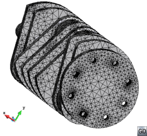
* ''Preserve geometrical features''. This is automatically achieved by the boundary constrained meshers, but it is not guaranteed at all by the types of meshers. This requirement is crucial for the final mesh to represent the shape of the domain precisely. For several kinds of numerical simulations, the presence of sharp edges and corners in the domain affects drastically the results, as they often govern the physical behavior of the process to be simulated. The importance of preserving sharp edges and corners to represent some domains can be appreciated in Figure [[#img-7|7]]. Part of the contours of a volume are shown in Figure [[#img-7|7]](a). The tetrahedral mesh of that volume generated without preserving the sharp edges of the input geometry is shown in Figure [[#img-7|7]](b). | * ''Preserve geometrical features''. This is automatically achieved by the boundary constrained meshers, but it is not guaranteed at all by the types of meshers. This requirement is crucial for the final mesh to represent the shape of the domain precisely. For several kinds of numerical simulations, the presence of sharp edges and corners in the domain affects drastically the results, as they often govern the physical behavior of the process to be simulated. The importance of preserving sharp edges and corners to represent some domains can be appreciated in Figure [[#img-7|7]]. Part of the contours of a volume are shown in Figure [[#img-7|7]](a). The tetrahedral mesh of that volume generated without preserving the sharp edges of the input geometry is shown in Figure [[#img-7|7]](b). | ||
| + | <div id='img-7a'></div> | ||
| + | <div id='img-7b'></div> | ||
<div id='img-7'></div> | <div id='img-7'></div> | ||
| − | {| style="text-align: center; border: 1px solid #BBB; margin: 1em auto; width: 100%;max-width: 100%;" | + | {| class="floating_imageSCP" style="text-align: center; border: 1px solid #BBB; margin: 1em auto; width: 100%;max-width: 100%;" |
|- | |- | ||
| − | |[[Image:draft_Samper_249832658-biela_geom.png| | + | |[[Image:draft_Samper_249832658-monograph-biela_geom.png|240px|(a)]] |
| − | |[[Image:draft_Samper_249832658-biela_mesh.png| | + | |[[Image:draft_Samper_249832658-monograph-biela_mesh.png|240px|(b)]] |
| + | |- style="text-align: center; font-size: 75%;" | ||
| + | | (a) | ||
| + | | (b) | ||
|- style="text-align: center; font-size: 75%;" | |- style="text-align: center; font-size: 75%;" | ||
| colspan="2" | '''Figure 7:''' '''(a)''' View of a part of the contours of a mechanical piece. '''(b)''' Tetrahedral mesh of the mechanical part generated without preserving the sharp edges of the input geometry. | | colspan="2" | '''Figure 7:''' '''(a)''' View of a part of the contours of a mechanical piece. '''(b)''' Tetrahedral mesh of the mechanical part generated without preserving the sharp edges of the input geometry. | ||
| Line 243: | Line 281: | ||
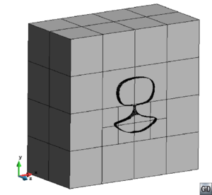
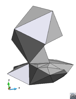
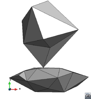
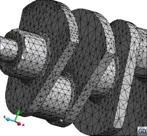
* ''Allow to skip given details of the domain''. This requirement is somehow complementary to the previous one. What it means is that the mesher must be not constrained in some regions. The definition of the geometrical domains includes often very thin or small entities in given parts. The reason for the size of these entities may be the size of the part of the domain represented itself, but the presence of these small entities often responds to the application of a given tangency criteria for the geometrical definition, or they are just the result of some geometrical operation previously done (intersections, Boolean operations, etc.). The basic idea of this requirement is that the sizes of the geometrical entities used to define the contours of the domain are not necessary related to the mesh size needed for the simulation. In the Figure [[#img-8|8]], an example is shown where the triangles generated from a patch of surfaces skipping the inner lines between them are much larger than the size of some of the surfaces of the patch. Clearly the simulation should not need such thin triangles in the regions where the surfaces are so thin. | * ''Allow to skip given details of the domain''. This requirement is somehow complementary to the previous one. What it means is that the mesher must be not constrained in some regions. The definition of the geometrical domains includes often very thin or small entities in given parts. The reason for the size of these entities may be the size of the part of the domain represented itself, but the presence of these small entities often responds to the application of a given tangency criteria for the geometrical definition, or they are just the result of some geometrical operation previously done (intersections, Boolean operations, etc.). The basic idea of this requirement is that the sizes of the geometrical entities used to define the contours of the domain are not necessary related to the mesh size needed for the simulation. In the Figure [[#img-8|8]], an example is shown where the triangles generated from a patch of surfaces skipping the inner lines between them are much larger than the size of some of the surfaces of the patch. Clearly the simulation should not need such thin triangles in the regions where the surfaces are so thin. | ||
| + | <div id='img-8a'></div> | ||
| + | <div id='img-8b'></div> | ||
<div id='img-8'></div> | <div id='img-8'></div> | ||
| − | {| style="text-align: center; border: 1px solid #BBB; margin: 1em auto; width: 100%;max-width: 100%;" | + | {| class="floating_imageSCP" style="text-align: center; border: 1px solid #BBB; margin: 1em auto; width: 100%;max-width: 100%;" |
|- | |- | ||
| − | |[[Image:draft_Samper_249832658-rjump_geom.png| | + | |[[Image:draft_Samper_249832658-monograph-rjump_geom.png|240px|(a)]] |
| − | |[[Image:draft_Samper_249832658-rjump_mesh.png| | + | |[[Image:draft_Samper_249832658-monograph-rjump_mesh.png|240px|(b)]] |
| + | |- style="text-align: center; font-size: 75%;" | ||
| + | | (a) | ||
| + | | (b) | ||
|- style="text-align: center; font-size: 75%;" | |- style="text-align: center; font-size: 75%;" | ||
| colspan="2" | '''Figure 8:''' '''(a)''' Zoom of a patch of surfaces representing a mechanical part. '''(b)''' Triangle mesh of the patch of surfaces shown in (a). | | colspan="2" | '''Figure 8:''' '''(a)''' Zoom of a patch of surfaces representing a mechanical part. '''(b)''' Triangle mesh of the patch of surfaces shown in (a). | ||
| Line 273: | Line 316: | ||
<div id='img-9'></div> | <div id='img-9'></div> | ||
| − | {| style="text-align: center; border: 1px solid #BBB; margin: 1em auto; width: | + | {| class="floating_imageSCP" style="text-align: center; border: 1px solid #BBB; margin: 1em auto; width: 100%;max-width: 100%;" |
|- | |- | ||
| − | |[[Image:draft_Samper_249832658-model_sail.png|300px|2D example of a surface mesh (gray lines) conformal with an inner line of the surface (dotted line).]] | + | |[[Image:draft_Samper_249832658-monograph-model_sail.png|300px|2D example of a surface mesh (gray lines) conformal with an inner line of the surface (dotted line).]] |
|- style="text-align: center; font-size: 75%;" | |- style="text-align: center; font-size: 75%;" | ||
| colspan="1" | '''Figure 9:''' 2D example of a surface mesh (gray lines) conformal with an inner line of the surface (dotted line). | | colspan="1" | '''Figure 9:''' 2D example of a surface mesh (gray lines) conformal with an inner line of the surface (dotted line). | ||
| Line 282: | Line 325: | ||
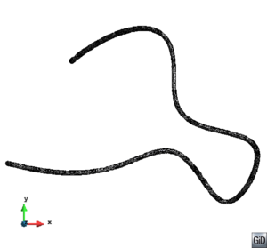
* Mesh in a conformal way a model with volumes and surfaces or lines connected to them. A case of two volumes connected by a surface is depicted in Figure [[#img-10|10]]. The mesh of the volumes and the surface must be conformal in the contact lines between them. This case can be also meshed by generating separately the volume meshes with the octree mesher, and afterwards mesh the surface using other meshing algorithms. This would not take profit on the advantages of meshing the whole model at once. | * Mesh in a conformal way a model with volumes and surfaces or lines connected to them. A case of two volumes connected by a surface is depicted in Figure [[#img-10|10]]. The mesh of the volumes and the surface must be conformal in the contact lines between them. This case can be also meshed by generating separately the volume meshes with the octree mesher, and afterwards mesh the surface using other meshing algorithms. This would not take profit on the advantages of meshing the whole model at once. | ||
| + | <div id='img-10a'></div> | ||
| + | <div id='img-10b'></div> | ||
<div id='img-10'></div> | <div id='img-10'></div> | ||
| − | {| style="text-align: center; border: 1px solid #BBB; margin: 1em auto; width: 100%;max-width: 100%;" | + | {| class="floating_imageSCP" style="text-align: center; border: 1px solid #BBB; margin: 1em auto; width: 100%;max-width: 100%;" |
|- | |- | ||
| − | |[[Image:draft_Samper_249832658-inner_surfaces_geom.png| | + | |[[Image:draft_Samper_249832658-monograph-inner_surfaces_geom.png|240px|(a)]] |
| − | |[[Image:draft_Samper_249832658-inner_surfaces_mesh.png| | + | |[[Image:draft_Samper_249832658-monograph-inner_surfaces_mesh.png|240px|(b)]] |
| + | |- style="text-align: center; font-size: 75%;" | ||
| + | | (a) | ||
| + | | (b) | ||
|- style="text-align: center; font-size: 75%;" | |- style="text-align: center; font-size: 75%;" | ||
| colspan="2" | '''Figure 10:''' '''(a)''' Example of a model containing two volumes (in blue) and a surface (in grey) connecting them. '''(b)''' A conformal mesh of the model considering the volumes and the surface mesh. | | colspan="2" | '''Figure 10:''' '''(a)''' Example of a model containing two volumes (in blue) and a surface (in grey) connecting them. '''(b)''' A conformal mesh of the model considering the volumes and the surface mesh. | ||
| Line 293: | Line 341: | ||
* Mesh patches of surface entities together preserving features, but skipping the inner line entities between them if needed. The entities to be skipped could be detected automatically following a given smoothness criteria, or under user demand. Figure [[#img-8|8]] shows an example of triangle mesh representing a collection of surface entities, but skipping the inner line entities. | * Mesh patches of surface entities together preserving features, but skipping the inner line entities between them if needed. The entities to be skipped could be detected automatically following a given smoothness criteria, or under user demand. Figure [[#img-8|8]] shows an example of triangle mesh representing a collection of surface entities, but skipping the inner line entities. | ||
| − | * If the patches of surfaces are not topologically connected, the proposed method could act as a CAD cleaning tool, as it could extract a continuous manifold surface mesh from a collection of surface entities with gaps or overlaps. The extraction of surface skin meshes from a volume discretization has been used in | + | * If the patches of surfaces are not topologically connected, the proposed method could act as a CAD cleaning tool, as it could extract a continuous manifold surface mesh from a collection of surface entities with gaps or overlaps. The extraction of surface skin meshes from a volume discretization has been used in <span id='citeF-8'></span>[[#cite-8|[8]]] and <span id='citeF-9'></span>[[#cite-9|[9]]], and it is interesting for CAD cleaning, as well as for boolean operations involving non-watertight geometries. The preservation of geometrical features is essential for these purposes. |
==1.3 Structure of the monography== | ==1.3 Structure of the monography== | ||
| Line 311: | Line 359: | ||
* Geometrical intersections (Section [[#3.4 Geometrical intersections|3.4]]). As the geometrical intersections are crucial for some of the algorithms presented, this section analyzes them deeply and studies the pathological configurations that may occur. | * Geometrical intersections (Section [[#3.4 Geometrical intersections|3.4]]). As the geometrical intersections are crucial for some of the algorithms presented, this section analyzes them deeply and studies the pathological configurations that may occur. | ||
| − | ''Chapter [[#4 Coloring algorithm|4]]: Coloring algorithm''. The coloring process determines where a point in space is topologically: it determines if it is outside the domain, inside a given volume, or onto an interface between volumes. This is one of the main operations involved in the presented mesher and can be understood as an auxiliary algorithm for the meshing itself, so a whole chapter is devoted to it. In this chapter different approaches to solve the coloring problem are studied (Section [[#4.1 Coloring strategies|4.1]]), and a new algorithm based in the ray casting technique is exposed (Section [[#4.2 Ray casting-based proposed technique|4.2]]). The implementation of this algorithm is presented in Section [[#4.3 Implementation of nodes coloring algorithm|4.3]]. | + | * ''Chapter [[#4 Coloring algorithm|4]]: Coloring algorithm''. The coloring process determines where a point in space is topologically: it determines if it is outside the domain, inside a given volume, or onto an interface between volumes. This is one of the main operations involved in the presented mesher and can be understood as an auxiliary algorithm for the meshing itself, so a whole chapter is devoted to it. In this chapter different approaches to solve the coloring problem are studied (Section [[#4.1 Coloring strategies|4.1]]), and a new algorithm based in the ray casting technique is exposed (Section [[#4.2 Ray casting-based proposed technique|4.2]]). The implementation of this algorithm is presented in Section [[#4.3 Implementation of nodes coloring algorithm|4.3]]. |
| − | ''Chapter [[#5 Octree based mesher|5]]: Octree based mesher''. This chapter focuses on the new meshing algorithm itself. After an introduction, where its main idea is highlighted (Section [[#5.1 Introduction|5.1]]), the algorithm for embedded (Section [[#5.2 Embedded mesher|5.2]]) and body-fitted (Section [[#5.3 Body-fitted mesher|5.3]]) meshes is detailed. | + | * ''Chapter [[#5 Octree based mesher|5]]: Octree based mesher''. This chapter focuses on the new meshing algorithm itself. After an introduction, where its main idea is highlighted (Section [[#5.1 Introduction|5.1]]), the algorithm for embedded (Section [[#5.2 Embedded mesher|5.2]]) and body-fitted (Section [[#5.3 Body-fitted mesher|5.3]]) meshes is detailed. |
| − | ''Chapter [[#6 Implementation aspects|6]]: Implementation aspects''. In this chapter all the implementation details for the meshing algorithm developed are explained. After some general aspects of the implementation (Section [[#6.1 General aspects|6.1]]), the implementation of the octree structure is analyzed (Section [[#6.2 Octree implementation|6.2]]). Sections [[#6.3 Generalized mesh size points|6.3]], [[#6.4 Sizes transition function|6.4]], and [[#6.5 Body-fitted mesher|6.5]] focus on the implementation of specific parts of the meshing algorithm itself. Some considerations on the parallel implementation of the mesher are pointed out in Section [[#6.6 Parallel processing|6.6]]. A list of the values of the parameters relevant for the mesher used in the presented implementation of the algorithm is detailed in Section [[#6.7 Parameters used|6.7]]. | + | * ''Chapter [[#6 Implementation aspects|6]]: Implementation aspects''. In this chapter all the implementation details for the meshing algorithm developed are explained. After some general aspects of the implementation (Section [[#6.1 General aspects|6.1]]), the implementation of the octree structure is analyzed (Section [[#6.2 Octree implementation|6.2]]). Sections [[#6.3 Generalized mesh size points|6.3]], [[#6.4 Sizes transition function|6.4]], and [[#6.5 Body-fitted mesher|6.5]] focus on the implementation of specific parts of the meshing algorithm itself. Some considerations on the parallel implementation of the mesher are pointed out in Section [[#6.6 Parallel processing|6.6]]. A list of the values of the parameters relevant for the mesher used in the presented implementation of the algorithm is detailed in Section [[#6.7 Parameters used|6.7]]. |
| − | ''Chapter [[#7 Examples|7]]: Examples''. In this chapter the results of some validation examples highlighting specific characteristics of the presented mesher are shown (Section [[#7.1 Validation examples|7.1]]). Sections [[#7.2 Racing car example|7.2]] and [[#7.3 Barcelona city model|7.3]] analyze the results of the meshing algorithm applied to real complex geometries under different configurations. | + | * ''Chapter [[#7 Examples|7]]: Examples''. In this chapter the results of some validation examples highlighting specific characteristics of the presented mesher are shown (Section [[#7.1 Validation examples|7.1]]). Sections [[#7.2 Racing car example|7.2]] and [[#7.3 Barcelona city model|7.3]] analyze the results of the meshing algorithm applied to real complex geometries under different configurations. |
| − | ''Chapter [[#8 Conclusions and future lines|8]]: Conclusions and future research lines''. This chapter lists the conclusions of the presented work (Section [[#8.1 Conclusions|8.1]]) and proposes some futures lines of research (Section [[#8.2 Future research lines|8.2]]). | + | * ''Chapter [[#8 Conclusions and future lines|8]]: Conclusions and future research lines''. This chapter lists the conclusions of the presented work (Section [[#8.1 Conclusions|8.1]]) and proposes some futures lines of research (Section [[#8.2 Future research lines|8.2]]). |
| − | ''Appendix A: Profiling tables and complete data of examples''. In this appendix, tables with all the profiling data concerning times and memory for the whole configurations used in the examples run to validate the meshing algorithm are provided. | + | * ''Appendix A: Profiling tables and complete data of examples''. In this appendix, tables with all the profiling data concerning times and memory for the whole configurations used in the examples run to validate the meshing algorithm are provided. |
It is highlighted that, although the meshing algorithms presented are directly applied to volume meshing, most of the geometrical operations are applicable (with slight modifications) to surface meshing in 2D cases. Taking into account that some concepts are much more clear to understand from a 2D scheme (especially when dealing with geometry), in this monography 2D examples are used sometimes to illustrate some of the concepts explained. | It is highlighted that, although the meshing algorithms presented are directly applied to volume meshing, most of the geometrical operations are applicable (with slight modifications) to surface meshing in 2D cases. Taking into account that some concepts are much more clear to understand from a 2D scheme (especially when dealing with geometry), in this monography 2D examples are used sometimes to illustrate some of the concepts explained. | ||
| − | |||
| − | |||
=2 State of the art on mesh generation= | =2 State of the art on mesh generation= | ||
| Line 333: | Line 379: | ||
==2.1 Mesh types== | ==2.1 Mesh types== | ||
| − | There are two main families of meshers depending on the kind of mesh they generate: structured and unstructured <span id='citeF- | + | There are two main families of meshers depending on the kind of mesh they generate: structured and unstructured <span id='citeF-10'></span>[[#cite-10|[10]]]. Actually, a third kind of meshers can be classified as semi-structured ones. A structured mesh is defined as a mesh which all inner nodes have the same degree (the degree of a node is the number of elements owning it), while the nodes of an unstructured mesh have different degrees. Semi-structured meshes can only be applied to topologically prismatic geometries, and they basically repeat the structure of an unstructured mesh (in the tops of the prismatic shape) in different layers following the structured direction. An example of this kinds of mesh is shown in Figure [[#img-11|11]]. |
| − | Unstructured meshers <span id='citeF- | + | Unstructured meshers <span id='citeF-11'></span><span id='citeF-5'></span><span id='citeF-12'></span>[[#cite-11|[11,5,12]]] can be divided in three main families: ''advancing front'', ''Delaunay'' and ''space decomposition'' methods. |
In the following sections, the main characteristics of these methods as well as their main advantages and drawbacks are detailed, focusing on the requirements defined in section [[#1.2 Objectives|1.2]]. The aim of this chapter is to highlight which of those requirements are covered by each meshing method, so the algorithms are not deeply detailed and only their main characteristics are pointed out. | In the following sections, the main characteristics of these methods as well as their main advantages and drawbacks are detailed, focusing on the requirements defined in section [[#1.2 Objectives|1.2]]. The aim of this chapter is to highlight which of those requirements are covered by each meshing method, so the algorithms are not deeply detailed and only their main characteristics are pointed out. | ||
<div id='img-11'></div> | <div id='img-11'></div> | ||
| − | {| style="text-align: center; border: 1px solid #BBB; margin: 1em auto; width: 100%;max-width: 100%;" | + | {| class="floating_imageSCP" style="text-align: center; border: 1px solid #BBB; margin: 1em auto; width: 100%;max-width: 100%;" |
|- | |- | ||
| − | | | + | | |
| − | | | + | {| style="text-align: center; margin: 1em auto;min-width:50%;width:100%;" |
|- | |- | ||
| − | | | + | | [[Image:draft_Samper_249832658-monograph-structured_triangle.png|300px|Figures/chapter_stateoftheart/structured_triangle]] |
| + | | [[Image:draft_Samper_249832658-monograph-unstructured_triangle.png|300px|Figures/chapter_stateoftheart/unstructured_triangle]] | ||
| + | | [[Image:draft_Samper_249832658-monograph-prism_mesh.png|300px|Figures/chapter_stateoftheart/prism_mesh]] | ||
| + | |- | ||
| + | | (a) | ||
| + | | (b) | ||
| + | | (c) | ||
| + | |||
| + | |} | ||
| + | |||
| + | |- | ||
| + | |||
|- style="text-align: center; font-size: 75%;" | |- style="text-align: center; font-size: 75%;" | ||
| − | | colspan=" | + | | colspan="1" | '''Figure 11:''' Examples of different types of mesh'''(a)''' Structured triangle mesh. '''(b)''' Unstructured triangle mesh. '''(b)''' Semi-structured prism mesh. |
|} | |} | ||
==2.2 Structured meshers== | ==2.2 Structured meshers== | ||
| − | Structured and semi-structured meshers often get as input data the position of the nodes in the contours of the domain, and generate the inner nodes positions from a given interpolation <span id='citeF- | + | Structured and semi-structured meshers often get as input data the position of the nodes in the contours of the domain, and generate the inner nodes positions from a given interpolation <span id='citeF-10'></span><span id='citeF-12'></span><span id='citeF-4'></span>[[#cite-10|[10,12,4]]]. The quality of the final mesh obtained is directly related to the kind of interpolation used and the degree of distortion of the contours of the domain, so a minimum level of element quality cannot be guaranteed for arbitrary domains. However, for good shaped volumes and uniform sizes distributions these methods provide with very good quality meshes. |
The main advantages of structured meshers are: | The main advantages of structured meshers are: | ||
| Line 361: | Line 418: | ||
On the other hand, these meshers have some important drawbacks: | On the other hand, these meshers have some important drawbacks: | ||
| − | * ''Need of specific topology for the input data''. The main problem of this kind of meshers remains in a requirement for the input data: they need a specific topology for the geometrical definition of the contours of the domain. As an example, to generate a structured mesh of hexahedra, the input geometry must be topologically an hexahedra. This means it has to be a volume with 6 contour surfaces, and each one of their must have 4 contour lines. This requirement makes impossible to use this kind of meshers for arbitrary geometries with complex topology. A family of methods has been proposed that are able to skip this problem <span id='citeF- | + | * ''Need of specific topology for the input data''. The main problem of this kind of meshers remains in a requirement for the input data: they need a specific topology for the geometrical definition of the contours of the domain. As an example, to generate a structured mesh of hexahedra, the input geometry must be topologically an hexahedra. This means it has to be a volume with 6 contour surfaces, and each one of their must have 4 contour lines. This requirement makes impossible to use this kind of meshers for arbitrary geometries with complex topology. A family of methods has been proposed that are able to skip this problem <span id='citeF-13'></span>[[#cite-13|[13]]]. They are basically based in decomposing the original domain to be meshed into different parts which do accomplish with the topology demanded by the mesher. Then, each of these parts can be meshed in a structured manner, so they are often referred as ''structured by blocks'' or ''multi-block'' meshers. Several implementations of these methods have been carried out <span id='citeF-11'></span><span id='citeF-10'></span>[[#cite-11|[11,10]]], but in practice they are meaningful for very specific domains only. Depending on the topology required by the mesher, some geometries are impossible to be decomposed in such this way, and even when this decomposition is possible, from complex original geometries is not obvious to generate this decomposition automatically. This often implies an extra pre-processing operation before using the mesher, which is the splitting (manually) of the domain in different parts. |
<div id='img-12'></div> | <div id='img-12'></div> | ||
| − | {| style="text-align: center; border: 1px solid #BBB; margin: 1em auto; width: | + | {| class="floating_imageSCP" style="text-align: center; border: 1px solid #BBB; margin: 1em auto; width: 100%;max-width: 100%;" |
|- | |- | ||
| − | |[[Image:draft_Samper_249832658-structured_distortion.png|360px|Example of a 2D structured quadrilateral mesh with a non-uniform size distribution. A high level of element distortion can be appreciated.]] | + | |[[Image:draft_Samper_249832658-monograph-structured_distortion.png|360px|Example of a 2D structured quadrilateral mesh with a non-uniform size distribution. A high level of element distortion can be appreciated.]] |
|- style="text-align: center; font-size: 75%;" | |- style="text-align: center; font-size: 75%;" | ||
| colspan="1" | '''Figure 12:''' Example of a 2D structured quadrilateral mesh with a non-uniform size distribution. A high level of element distortion can be appreciated. | | colspan="1" | '''Figure 12:''' Example of a 2D structured quadrilateral mesh with a non-uniform size distribution. A high level of element distortion can be appreciated. | ||
| Line 375: | Line 432: | ||
==2.3 Advancing front method== | ==2.3 Advancing front method== | ||
| − | The advancing front method <span id='citeF- | + | The advancing front method <span id='citeF-14'></span><span id='citeF-15'></span><span id='citeF-16'></span><span id='citeF-17'></span>[[#cite-14|[14,15,16,17]]] is a common technique for generating unstructured meshes. It gets a closed and oriented mesh of the boundary of the domain as input and mesh its inner part. The surface elements of this mesh are the ones in the ''active front'', and the algorithm can be summarized with the following points: |
* From each element in the front (face) a new volume element is generated. An optimal position of the node needed to build the element is obtained and the nodes and faces of the active front close to it are considered. The new element is build using a new node in the optimal position or an existing close node, depending on the resulting configuration: the new element should not intersect any one of the close already existing faces. | * From each element in the front (face) a new volume element is generated. An optimal position of the node needed to build the element is obtained and the nodes and faces of the active front close to it are considered. The new element is build using a new node in the optimal position or an existing close node, depending on the resulting configuration: the new element should not intersect any one of the close already existing faces. | ||
| Line 381: | Line 438: | ||
* These two steps are repeated until there are no faces in the active front. Then all the domain has been filled with volume elements. | * These two steps are repeated until there are no faces in the active front. Then all the domain has been filled with volume elements. | ||
| − | Although the advancing front is mainly used for generation of tetrahedral (or triangle in 2D) elements, some adaptations of the method have been done to generate other types of elements <span id='citeF- | + | Although the advancing front is mainly used for generation of tetrahedral (or triangle in 2D) elements, some adaptations of the method have been done to generate other types of elements <span id='citeF-18'></span>[[#cite-18|[18]]], and even for generating particles for DEM simulations <span id='citeF-19'></span>[[#cite-19|[19]]]. The present work is focused in tetrahedra mesh generation. There are several possible implementations of the advancing front method <span id='citeF-11'></span>[[#cite-11|[11]]] depending on the way of creating the new elements from a face of the front, the way of considering the mesh desired size in the inner part of the domain, or the order in which the faces of the front are processed, among others. In special, much work have been done in order to improve the efficiency in evaluating the desired mesh size in a specific region of the domain, and control a smooth size transition in the final mesh. This is one of the strong points of advancing front techniques, as the creation of each element can fit very well the desired mesh requirements. Different approaches use a background grid to set the mesh desired size <span id='citeF-16'></span><span id='citeF-15'></span><span id='citeF-20'></span><span id='citeF-21'></span>[[#cite-16|[16,15,20,21]]], or sources from which the desired mesh size vary following a given function <span id='citeF-22'></span>[[#cite-22|[22]]], which provides with a very smooth transition between element sizes. A combination of different methods can be used in order to improve accuracy and reach an efficient implementation of the method <span id='citeF-23'></span>[[#cite-23|[23]]]. However, independent of the implementation, one can identify some general advantages and disadvantages of advancing front based techniques. The main advantages are: |
* ''Good quality meshes''. In the advancing front method, each new element is created connecting a face of the active front with a new node or an existing one. This choice is done based on an optimal position for this new node in order to get the best element (in terms of quality) taking into account the desired size of the mesh in that region. This methodology for creating the elements gives high quality elements in the final mesh, even before any smoothing process. | * ''Good quality meshes''. In the advancing front method, each new element is created connecting a face of the active front with a new node or an existing one. This choice is done based on an optimal position for this new node in order to get the best element (in terms of quality) taking into account the desired size of the mesh in that region. This methodology for creating the elements gives high quality elements in the final mesh, even before any smoothing process. | ||
| Line 389: | Line 446: | ||
* ''Good control on the size transitions''. As explained before, each new element is created from an existing face and an optimal position of the node to create the element from the face. Considering the desired size for the final mesh in the region where the face is, and the size of the face itself, the size transitions from one part of the mesh to another is totally controlled. | * ''Good control on the size transitions''. As explained before, each new element is created from an existing face and an optimal position of the node to create the element from the face. Considering the desired size for the final mesh in the region where the face is, and the size of the face itself, the size transitions from one part of the mesh to another is totally controlled. | ||
| − | * ''Parallelizable''. The creation of each new element using the advancing front method is clearly local. The geometrical and topological checks needed to create the new element only take into account the nodes and faces inside a specific radius of influence of the face the new element is created from. This aspect makes totally independent the creation of an element from the creation of another element which is far enough. Although it is not obvious to implement an efficient parallel version of the advancing front method, at least the element generation method is local enough to make the implementation affordable. <span id='citeF- | + | * ''Parallelizable''. The creation of each new element using the advancing front method is clearly local. The geometrical and topological checks needed to create the new element only take into account the nodes and faces inside a specific radius of influence of the face the new element is created from. This aspect makes totally independent the creation of an element from the creation of another element which is far enough. Although it is not obvious to implement an efficient parallel version of the advancing front method, at least the element generation method is local enough to make the implementation affordable. <span id='citeF-24'></span>[[#cite-24|[24]]] proposed a first octree subdivision of the domain, and then apply the advancing front technique in each of the cells of the octree, seaming afterwards the interface parts between cells. |
The main drawbacks of the advancing front method are: | The main drawbacks of the advancing front method are: | ||
| Line 403: | Line 460: | ||
==2.4 Delaunay method== | ==2.4 Delaunay method== | ||
| − | A Delaunay mesh is defined as a mesh which elements accomplish the Delaunay condition: the circumcircle (in 2D case) or the circumscribed sphere (in 3D case) of any element has no node from the mesh inside <span id='citeF- | + | A Delaunay mesh is defined as a mesh which elements accomplish the Delaunay condition: the circumcircle (in 2D case) or the circumscribed sphere (in 3D case) of any element has no node from the mesh inside <span id='citeF-10'></span>[[#cite-10|[10]]]. Given a cloud of points, a Delaunay triangulation can always be created from their Dirichlet tesselation connecting them with a set of triangles (in 2D) or tetrahedra (in 3D) without adding any extra node <span id='citeF-10'></span>[[#cite-10|[10]]]. |
| − | The Delaunay meshing methods [ | + | The Delaunay meshing methods <span id='citeF-12'></span><span id='citeF-25'></span><span id='citeF-5'></span><span id='citeF-11'></span>[[#cite-12|[12,25,5,11]]] depart from the contour of the domain and generate the Delaunay triangulation of its nodes. This mesh is the convex hull of the domain to be meshed. Although it is already a mesh, its elements may have a low quality, or may not fit with the desired mesh size in that region of the domain: these are the ''bad elements''. The following strategy is applied recursively to all the bad elements: |
| − | * A node is created in the centroid of the element. Some strategies allow the creation of the new node at the edges or faces of the elements <span id='citeF- | + | * A node is created in the centroid of the element. Some strategies allow the creation of the new node at the edges or faces of the elements <span id='citeF-26'></span>[[#cite-26|[26]]] in order to improve the quality of the elements respecting the contours of the domain. |
* All the elements of the mesh which circumscribed sphere (or circumcircle in 2D) includes the new node are deleted. Note that a void region is created containing the new node inside. | * All the elements of the mesh which circumscribed sphere (or circumcircle in 2D) includes the new node are deleted. Note that a void region is created containing the new node inside. | ||
* A Delaunay triangulation is created with the new node and the contour nodes of this void region. | * A Delaunay triangulation is created with the new node and the contour nodes of this void region. | ||
| − | This procedure leads to a Delaunay mesh (accomplishing the Delaunay condition), but this does not guarantee a given level of quality by itself. Often, some elements can present very low quality (especially in 3D cases). These elements may have null volume and are called ''slivers''. Even if its volume is equal to zero, they can accomplish the Delaunay condition. For this reason, it is common to relax the Delaunay condition in some regions in order to avoid quality problems <span id='citeF- | + | This procedure leads to a Delaunay mesh (accomplishing the Delaunay condition), but this does not guarantee a given level of quality by itself. Often, some elements can present very low quality (especially in 3D cases). These elements may have null volume and are called ''slivers''. Even if its volume is equal to zero, they can accomplish the Delaunay condition. For this reason, it is common to relax the Delaunay condition in some regions in order to avoid quality problems <span id='citeF-27'></span>[[#cite-27|[27]]]. |
The main advantages of this method are: | The main advantages of this method are: | ||
| Line 421: | Line 478: | ||
The main drawbacks of the Delaunay method are: | The main drawbacks of the Delaunay method are: | ||
| − | * ''Naturally not constrained''. Delaunay methods use the representation of the contour of the domain as an initial configuration for the insertion of nodes procedure, but the final mesh boundaries are not guaranteed to be constrained with that contour. Some strategies can be applied <span id='citeF- | + | * ''Naturally not constrained''. Delaunay methods use the representation of the contour of the domain as an initial configuration for the insertion of nodes procedure, but the final mesh boundaries are not guaranteed to be constrained with that contour. Some strategies can be applied <span id='citeF-28'></span><span id='citeF-29'></span><span id='citeF-30'></span>[[#cite-28|[28,29,30]]] in order to guarantee that the nodes in the initial contours will lay on the contour of the final mesh, or even a constrained condition in the faces of the initial contour, but these modifications reduce the performance and robustness of the method. Furthermore, if there are huge different mesh desired sizes in the domain, these strategies are not very robust. |
| − | * ''Requires watertight input geometry''. As in the advancing front method, the contours of the domain are required to be watertight. Actually, a strategy could be followed to treat non-watertight geometries. It is based on generating the first mesh (the convex hull in the traditional Delaunay methods) using only the nodes of the contours, with an automatic recognition of the boundaries: the so called ''alpha-shape method'' <span id='citeF- | + | * ''Requires watertight input geometry''. As in the advancing front method, the contours of the domain are required to be watertight. Actually, a strategy could be followed to treat non-watertight geometries. It is based on generating the first mesh (the convex hull in the traditional Delaunay methods) using only the nodes of the contours, with an automatic recognition of the boundaries: the so called ''alpha-shape method'' <span id='citeF-31'></span>[[#cite-31|[31]]]. This would indeed generate a volume mesh from a non-watertight geometry, but there is no enough control in the boundaries recognition to ensure that mesh correctly represents the topology of the domain. |
| − | * ''Not naturally parallelizable''. The check of the Delaunay condition of an element requires taking into account all the mesh entities participating in the circumscribed sphere of the element. As its radius depends on the position of the nodes of the element (cannot be bounded a priori), the treatment of one element can involve the whole mesh in some configurations. This implies a hard dependency ranging from an element to the whole mesh, so a parallel implementation of the method is not obvious. However, some parallel implementations (mainly for shared memory paradigm) of the Delaunay method have been carried out, <span id='citeF- | + | * ''Not naturally parallelizable''. The check of the Delaunay condition of an element requires taking into account all the mesh entities participating in the circumscribed sphere of the element. As its radius depends on the position of the nodes of the element (cannot be bounded a priori), the treatment of one element can involve the whole mesh in some configurations. This implies a hard dependency ranging from an element to the whole mesh, so a parallel implementation of the method is not obvious. However, some parallel implementations (mainly for shared memory paradigm) of the Delaunay method have been carried out, <span id='citeF-32'></span>[[#cite-32|[32]]] or <span id='citeF-33'></span>[[#cite-33|[33]]]. |
==2.5 Space decomposition methods== | ==2.5 Space decomposition methods== | ||
| Line 433: | Line 490: | ||
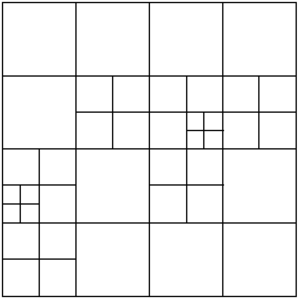
* ''Bin'': a bin structure provides with an homogeneous grid as the space decomposition formed by regular cells (squares in 2D or cubes in 3D). A graphical view of a 2D bin is shown in Figure [[#img-13|13]](a). | * ''Bin'': a bin structure provides with an homogeneous grid as the space decomposition formed by regular cells (squares in 2D or cubes in 3D). A graphical view of a 2D bin is shown in Figure [[#img-13|13]](a). | ||
| − | * ''Octree'': an octree (quadtree for the 2D case) is basically a hierarchical spatial structure that partitions the 3D space into regular cells <span id='citeF- | + | * ''Octree'': an octree (quadtree for the 2D case) is basically a hierarchical spatial structure that partitions the 3D space into regular cells <span id='citeF-34'></span>[[#cite-34|[34]]]. These cells can be refined in given zones of the domain. A graphical view of a quadtree is shown in Figure [[#img-13|13]](b). A more detailed definition of the octree structure is given in Section [[#3.2 Octree structure|3.2]]. |
| + | <div id='img-13a'></div> | ||
| + | <div id='img-13b'></div> | ||
<div id='img-13'></div> | <div id='img-13'></div> | ||
| − | {| style="text-align: center; border: 1px solid #BBB; margin: 1em auto; width: 100%;max-width: 100%;" | + | {| class="floating_imageSCP" style="text-align: center; border: 1px solid #BBB; margin: 1em auto; width: 100%;max-width: 100%;" |
|- | |- | ||
| − | |[[Image:draft_Samper_249832658-bin.png| | + | |[[Image:draft_Samper_249832658-monograph-bin.png|180px|(a)]] |
| − | |[[Image:draft_Samper_249832658-quadtree.png| | + | |[[Image:draft_Samper_249832658-monograph-quadtree.png|180px|(b)]] |
| + | |- style="text-align: center; font-size: 75%;" | ||
| + | | (a) | ||
| + | | (b) | ||
|- style="text-align: center; font-size: 75%;" | |- style="text-align: center; font-size: 75%;" | ||
| colspan="2" | '''Figure 13:''' 2D examples of typical structures used in space decomposition based meshing algorithms. '''(a)''' Bin. '''(b)''' Quadtree. | | colspan="2" | '''Figure 13:''' 2D examples of typical structures used in space decomposition based meshing algorithms. '''(a)''' Bin. '''(b)''' Quadtree. | ||
|} | |} | ||
| − | The bin structure is suitable for homogeneous discretizations. It is common to use an octree structure as the regular grid (which gives the name of the family of methods), because it is more flexible for mesh generation purposes, as domains to be meshed and desired mesh sizes are commonly non-homogeneous. Octree-based meshers were pioneered by Yerry and Shephard in <span id='citeF- | + | The bin structure is suitable for homogeneous discretizations. It is common to use an octree structure as the regular grid (which gives the name of the family of methods), because it is more flexible for mesh generation purposes, as domains to be meshed and desired mesh sizes are commonly non-homogeneous. Octree-based meshers were pioneered by Yerry and Shephard in <span id='citeF-35'></span>[[#cite-35|[35]]] and, since then, several approaches have been proposed <span id='citeF-36'></span><span id='citeF-37'></span><span id='citeF-38'></span><span id='citeF-39'></span><span id='citeF-40'></span><span id='citeF-41'></span><span id='citeF-42'></span>[[#cite-36|[36,37,38,39,40,41,42]]]. |
| − | The octree structure was thought for the first time for space searching purposes <span id='citeF- | + | The octree structure was thought for the first time for space searching purposes <span id='citeF-34'></span>[[#cite-34|[34]]], and the specific topology of the spatial decomposition it represents (detailed in Section [[#3.2 Octree structure|3.2]]) gives several advantages for mesh generation. Somehow, an octree can be considered a mesh itself (it can be thought as a non-conformal hexahedra mesh), so it is really natural to build a mesh from it. |
Although several algorithms have been proposed parting from the octree-based family of methods, almost all of them follow three main steps: | Although several algorithms have been proposed parting from the octree-based family of methods, almost all of them follow three main steps: | ||
| Line 454: | Line 516: | ||
* Fit somehow the boundaries of the domain. | * Fit somehow the boundaries of the domain. | ||
| − | Concerning the first step, as it has been pointed out before, the octree is the most common structure used for the space decomposition. From the theoretical point of view, all octrees are similar, but depending on the way the octree will be used, different implementations have been proposed by several authors <span id='citeF- | + | Concerning the first step, as it has been pointed out before, the octree is the most common structure used for the space decomposition. From the theoretical point of view, all octrees are similar, but depending on the way the octree will be used, different implementations have been proposed by several authors <span id='citeF-43'></span><span id='citeF-34'></span>[[#cite-43|[43,34]]] in order to improve the efficiency of the octree, the performance for searching processes, the optimization considering the memory needed to store it, etc... More details on the implementation of the octree are presented in Section [[#6.2 Octree implementation|6.2]]. |
| − | The generation of the elements of the final mesh from the octree is a simple process. It is based in creating the mesh elements directly from the ''octree cells'' (the definition of octree cell, as well as other octree related basic concepts are explained in detail in Section [[#3.2 Octree structure|3.2]]). Some of the existing methods apply different splitting patterns from the cells to get tetrahedra <span id='citeF- | + | The generation of the elements of the final mesh from the octree is a simple process. It is based in creating the mesh elements directly from the ''octree cells'' (the definition of octree cell, as well as other octree related basic concepts are explained in detail in Section [[#3.2 Octree structure|3.2]]). Some of the existing methods apply different splitting patterns from the cells to get tetrahedra <span id='citeF-35'></span><span id='citeF-44'></span><span id='citeF-37'></span>[[#cite-35|[35,44,37]]]. Other methods can get directly the cells of the octree as hexahedra elements of the final mesh (in cases where the final mesh is not needed to be conformal), or create transition elements when two neighbors present hanging nodes <span id='citeF-42'></span>[[#cite-42|[42]]]. <span id='citeF-40'></span>[[#cite-40|[40]]] proposes a different approach: create special cells where the octree is refined (where the neighbor elements are not conformal) and build the dual of the octree. The cells of it are directly the elements of the final mesh. With this approach a final mesh of conformal hexahedra is obtained automatically. |
The key difference of each method remains in the third step, which is the most complex one. As the octree is a regular space decomposition, their cells do not fit exactly the contours of the domain to be meshed. Getting only the elements coming from the cells which are in the inner part of the domain (or even the ones intersecting its boundaries), the contours of the final mesh are staircase-like, so they are not able to represent smooth shapes with a given curvature. | The key difference of each method remains in the third step, which is the most complex one. As the octree is a regular space decomposition, their cells do not fit exactly the contours of the domain to be meshed. Getting only the elements coming from the cells which are in the inner part of the domain (or even the ones intersecting its boundaries), the contours of the final mesh are staircase-like, so they are not able to represent smooth shapes with a given curvature. | ||
| Line 464: | Line 526: | ||
* Get only the inner cells and fill somehow the empty space between them and the real contour of the domain. This family of methods profits from the main advantages of octree-based methods for the inner part of the domains, but presents the same limitations near the contours as the methods used to fill those empty spaces. | * Get only the inner cells and fill somehow the empty space between them and the real contour of the domain. This family of methods profits from the main advantages of octree-based methods for the inner part of the domains, but presents the same limitations near the contours as the methods used to fill those empty spaces. | ||
| − | * Project onto the contour of the domain the boundary nodes of the elements created from the inner cells using different techniques <span id='citeF- | + | * Project onto the contour of the domain the boundary nodes of the elements created from the inner cells using different techniques <span id='citeF-36'></span><span id='citeF-39'></span>[[#cite-36|[36,39]]]. This strategy warps the nodes coming from the octree, so the shape of the octree changes, but its topology remains the same. <span id='citeF-42'></span>[[#cite-42|[42]]] proposes a pillowing technique near the contours to avoid bad shaped elements (hexahedra) after mapping the nodes. |
| − | * Move some nodes and split the elements intersecting the contours of the domain in order to represent it precisely <span id='citeF- | + | * Move some nodes and split the elements intersecting the contours of the domain in order to represent it precisely <span id='citeF-37'></span>[[#cite-37|[37]]]. |
| − | Although these methods achieve the smooth representation of the contours, they have to follow specific strategies to preserve the geometrical features (corners or sharp edges). [ | + | Although these methods achieve the smooth representation of the contours, they have to follow specific strategies to preserve the geometrical features (corners or sharp edges). <span id='citeF-41'></span>[[#cite-41|[41]]] proposes a re-tetrahedralization of the octants of the octree containing sharp edges using advancing front or Delaunay technique, taking into account the intersection points between the sharp edges and the octree cells. <span id='citeF-40'></span>[[#cite-40|[40]]] follows a strategy based on detecting which triangle from the input boundary the final nodes lay onto, and assuming that if two nodes lie onto two triangles connected by a sharp edge, there should be a sharp edge between those nodes of the final mesh. This strategy is not so robust, as it assumes that the sizes of the final elements is quite similar to the sizes of the triangles of the contour, so the triangles where two neighbor nodes of the final mesh lie onto are supposed to be neighbors connected by an edge. This is not a general situation. |
As it has been explained, several approaches have been proposed departing from the octree-based family of methods. Although each approach has its own characteristics, some common advantages can be detected: | As it has been explained, several approaches have been proposed departing from the octree-based family of methods. Although each approach has its own characteristics, some common advantages can be detected: | ||
| Line 504: | Line 566: | ||
As explained in Section [[#1.2.4 Surface meshing|1.2.4]], although the main objective of this work is to develop a new volume mesher, the methodology proposed is applicable to generate meshes of 3D surfaces and lines not belonging to any volume. The case of lines is automatically solved with the special treatment of line elements in the volume mesher (Section [[#5.3.1 Forced edges|5.3.1]]), and some adaptations are maid to the volume mesher in order to mesh surfaces as it is explained on Section [[#5.3.10 Extension for surface meshing|5.3.10]]. | As explained in Section [[#1.2.4 Surface meshing|1.2.4]], although the main objective of this work is to develop a new volume mesher, the methodology proposed is applicable to generate meshes of 3D surfaces and lines not belonging to any volume. The case of lines is automatically solved with the special treatment of line elements in the volume mesher (Section [[#5.3.1 Forced edges|5.3.1]]), and some adaptations are maid to the volume mesher in order to mesh surfaces as it is explained on Section [[#5.3.10 Extension for surface meshing|5.3.10]]. | ||
| − | |||
| − | |||
=3 Basic concepts of the new mesher= | =3 Basic concepts of the new mesher= | ||
| Line 532: | Line 592: | ||
* ''Forced line entities''. These are line entities to be preserved in the final mesh. This means that the final tetrahedra mesh will have a connected path of edges identifiable as a linear mesh of each forced line entity. As an example, the line entities in Figure [[#img-14|14]](a) can be considered as forced line entities, as a path of connected edges representing it can be identified in the mesh shown in Figure [[#img-14|14]](b). Forced line entities can be part of the input boundaries or not. | * ''Forced line entities''. These are line entities to be preserved in the final mesh. This means that the final tetrahedra mesh will have a connected path of edges identifiable as a linear mesh of each forced line entity. As an example, the line entities in Figure [[#img-14|14]](a) can be considered as forced line entities, as a path of connected edges representing it can be identified in the mesh shown in Figure [[#img-14|14]](b). Forced line entities can be part of the input boundaries or not. | ||
| + | <div id='img-14a'></div> | ||
| + | <div id='img-14b'></div> | ||
<div id='img-14'></div> | <div id='img-14'></div> | ||
| − | {| style="text-align: center; border: 1px solid #BBB; margin: 1em auto; width: 100%;max-width: 100%;" | + | {| class="floating_imageSCP" style="text-align: center; border: 1px solid #BBB; margin: 1em auto; width: 100%;max-width: 100%;" |
|- | |- | ||
| − | |[[ | + | |[[Image:draft_Samper_249832658-monograph-sharp_edges_geom.png|240px|(a)]] |
| − | |[[ | + | |[[Image:draft_Samper_249832658-monograph-sharp_edges_mesh2.png|240px|(b)]] |
| + | |- style="text-align: center; font-size: 75%;" | ||
| + | | (a) | ||
| + | | (b) | ||
|- style="text-align: center; font-size: 75%;" | |- style="text-align: center; font-size: 75%;" | ||
| colspan="2" | '''Figure 14:''' '''(a)''' Contours of a volume highlighting some of its forced line entities. '''(b)''' View of the tetrahedra mesh of the volume highlighting the sharp edges corresponding to the forced line entities in (a). | | colspan="2" | '''Figure 14:''' '''(a)''' Contours of a volume highlighting some of its forced line entities. '''(b)''' View of the tetrahedra mesh of the volume highlighting the sharp edges corresponding to the forced line entities in (a). | ||
| Line 584: | Line 649: | ||
<div id='img-15'></div> | <div id='img-15'></div> | ||
| − | {| style="text-align: center; border: 1px solid #BBB; margin: 1em auto; width: 100%;max-width: 100%;" | + | {| class="floating_imageSCP" style="text-align: center; border: 1px solid #BBB; margin: 1em auto; width: 100%;max-width: 100%;" |
|- | |- | ||
| − | | | + | | |
| − | | | + | {| style="text-align: center; margin: 1em auto;min-width:50%;width:100%;" |
|- | |- | ||
| − | | | + | | [[Image:draft_Samper_249832658-monograph-root.png|300px|Figures/chapter_concepts/root]] |
| + | | [[Image:draft_Samper_249832658-monograph-root_subdivided.png|300px|Figures/chapter_concepts/root_subdivided]] | ||
| + | | [[Image:draft_Samper_249832658-monograph-quadtree_refined.png|300px|Figures/chapter_concepts/quadtree_refined]] | ||
| + | |- | ||
| + | | (a) | ||
| + | | (b) | ||
| + | | (c) | ||
| + | |||
| + | |} | ||
| + | |||
| + | |- | ||
| + | |||
|- style="text-align: center; font-size: 75%;" | |- style="text-align: center; font-size: 75%;" | ||
| − | | colspan=" | + | | colspan="1" | '''Figure 15:''' Example of a quadtree structure. '''(a)''' The root cell of a quadtree. '''(b)''' Root cell subdivided in 4 cells. '''(c)''' Example of a quadtree refined 4 levels. |
|} | |} | ||
| − | An octree (quadtree in the 2D case) is basically a hierarchical spatial structure that partitions the space <span id='citeF- | + | An octree (quadtree in the 2D case) is basically a hierarchical spatial structure that partitions the space <span id='citeF-34'></span>[[#cite-34|[34]]]. The basic structure of an octree is the ''cell'', which is a cubic portion of space (square in the 2D case). Actually, the cell can be a parallelepiped (or parallelogram in 2D). In this work the octree used is an homogeneous one, which implies that the cells are regular parallelepipeds (cubes). From a first cell which is the bounding box of the space to be partitioned (the so called ''root'' of the octree), a successive subdivision can be performed, where each cell is subdivided in eight cells (four in 2D case). These eight cells are the ''sons'' of the cell they come from, which is their ''father''. Cells with no sons are called ''leaves''. |
In the Figure [[#img-15|15]] a graphical view of the root of a quadtree and different levels of refinement are shown. | In the Figure [[#img-15|15]] a graphical view of the root of a quadtree and different levels of refinement are shown. | ||
| Line 623: | Line 699: | ||
==3.3 Specific octree properties for mesh generation== | ==3.3 Specific octree properties for mesh generation== | ||
| − | As explained in previous sections, the octree structure was thought for the first time for space searching purposes <span id='citeF- | + | As explained in previous sections, the octree structure was thought for the first time for space searching purposes <span id='citeF-34'></span>[[#cite-34|[34]]]. In this section, the adaptations to the octree structure done in order to use it for mesh generation and its main properties to understand the algorithm are explained. |
The decision of using the octree for isotropic mesh generation leads to use an isotropic octree. This decision has an important relevance at the time of implementing the algorithm (as it will be seen in Section [[#6.2 Octree implementation|6.2]]). | The decision of using the octree for isotropic mesh generation leads to use an isotropic octree. This decision has an important relevance at the time of implementing the algorithm (as it will be seen in Section [[#6.2 Octree implementation|6.2]]). | ||
| Line 630: | Line 706: | ||
<div id='img-16'></div> | <div id='img-16'></div> | ||
| − | {| style="text-align: center; border: 1px solid #BBB; margin: 1em auto; width: 100%;max-width: 100%;" | + | {| class="floating_imageSCP" style="text-align: center; border: 1px solid #BBB; margin: 1em auto; width: 100%;max-width: 100%;" |
|- | |- | ||
| − | | | + | | |
| − | | | + | {| style="text-align: center; margin: 1em auto;min-width:50%;width:100%;" |
|- | |- | ||
| − | |[[Image:draft_Samper_249832658-isotropic_quadtree_nobalanced.png| | + | | [[Image:draft_Samper_249832658-monograph-nonisotropic_quadtree.png|300px|Figures/chapter_concepts/nonisotropic_quadtree]] |
| − | |[[Image:draft_Samper_249832658-isotropic_quadtree_balanced.png| | + | | [[Image:draft_Samper_249832658-monograph-isotropic_quadtree_nomiddle.png|300px|Figures/chapter_concepts/isotropic_quadtree_nomiddle]] |
| + | | [[Image:draft_Samper_249832658-monograph-isotropic_quadtree_nobalanced.png|300px|Figures/chapter_concepts/isotropic_quadtree_nobalanced]] | ||
| + | | [[Image:draft_Samper_249832658-monograph-isotropic_quadtree_balanced.png|300px|Figures/chapter_concepts/isotropic_quadtree_balanced]] | ||
| + | |- | ||
| + | | (a) | ||
| + | | (b) | ||
| + | | (c) | ||
| + | | (d) | ||
| + | |||
| + | |} | ||
| + | |||
| + | |- | ||
| + | |||
|- style="text-align: center; font-size: 75%;" | |- style="text-align: center; font-size: 75%;" | ||
| − | | colspan=" | + | | colspan="1" | '''Figure 16:''' Different kinds of quadtree. '''(a)''' Quadtree with a non-equilateral root, with a equidistant cell division criterion. '''(b)''' Quadtree with an equilateral root, with a non-equidistant cell division criterion. '''(c)''' Isotropic non-balanced quadtree. '''(d)''' Isotropic balanced quadtree. |
|} | |} | ||
| Line 650: | Line 738: | ||
<div id='img-17'></div> | <div id='img-17'></div> | ||
| − | {| style="text-align: center; border: 1px solid #BBB; margin: 1em auto; width: | + | {| class="floating_imageSCP" style="text-align: center; border: 1px solid #BBB; margin: 1em auto; width: 100%;max-width: 100%;" |
|- | |- | ||
| − | |[[Image:draft_Samper_249832658-octree_cells.png| | + | |[[Image:draft_Samper_249832658-monograph-octree_cells.png|240px|2D example where the three kinds of cells can be identified. The black curved line defines the contours of a domain formed by two surfaces (which are in contact), and the light gray lines represent the octree. Outer cells are the white ones, interface cells are marked with dots, and inner cells are colored in gray.]] |
|- style="text-align: center; font-size: 75%;" | |- style="text-align: center; font-size: 75%;" | ||
| colspan="1" | '''Figure 17:''' 2D example where the three kinds of cells can be identified. The black curved line defines the contours of a domain formed by two surfaces (which are in contact), and the light gray lines represent the octree. Outer cells are the white ones, interface cells are marked with dots, and inner cells are colored in gray. | | colspan="1" | '''Figure 17:''' 2D example where the three kinds of cells can be identified. The black curved line defines the contours of a domain formed by two surfaces (which are in contact), and the light gray lines represent the octree. Outer cells are the white ones, interface cells are marked with dots, and inner cells are colored in gray. | ||
| Line 672: | Line 760: | ||
<div id='img-18'></div> | <div id='img-18'></div> | ||
| − | {| style="text-align: center; border: 1px solid #BBB; margin: 1em auto; width: | + | {| class="floating_imageSCP" style="text-align: center; border: 1px solid #BBB; margin: 1em auto; width: 100%;max-width: 100%;" |
|- | |- | ||
| − | |[[Image:draft_Samper_249832658-octree_positions.png|300px|Octree positions of an octree cell. The cell is represented by the black lines.]] | + | |[[Image:draft_Samper_249832658-monograph-octree_positions.png|300px|Octree positions of an octree cell. The cell is represented by the black lines.]] |
|- style="text-align: center; font-size: 75%;" | |- style="text-align: center; font-size: 75%;" | ||
| colspan="1" | '''Figure 18:''' Octree positions of an octree cell. The cell is represented by the black lines. | | colspan="1" | '''Figure 18:''' Octree positions of an octree cell. The cell is represented by the black lines. | ||
| Line 682: | Line 770: | ||
<div id='img-19'></div> | <div id='img-19'></div> | ||
| − | {| style="text-align: center; border: 1px solid #BBB; margin: 1em auto; width: | + | {| class="floating_imageSCP" style="text-align: center; border: 1px solid #BBB; margin: 1em auto; width: 100%;max-width: 100%;" |
|- | |- | ||
| − | |[[Image:draft_Samper_249832658-octree_linear_positions.png| | + | |[[Image:draft_Samper_249832658-monograph-octree_linear_positions.png|210px|Linear octree positions of a part of an octree. White dots are center of cells, and black dots correspond to vertices of cells.]] |
|- style="text-align: center; font-size: 75%;" | |- style="text-align: center; font-size: 75%;" | ||
| colspan="1" | '''Figure 19:''' Linear octree positions of a part of an octree. White dots are center of cells, and black dots correspond to vertices of cells. | | colspan="1" | '''Figure 19:''' Linear octree positions of a part of an octree. White dots are center of cells, and black dots correspond to vertices of cells. | ||
| Line 701: | Line 789: | ||
Parting from a given octree configuration, there are several possible tetrahedra patterns to be applied in order to split it. One important consideration is that the pattern chosen must fill the space with tetrahedra in a conformal way: it must not leave hanging nodes. A hanging node is a node lying on an element not being a vertex of it (it is on an edge or a face). | Parting from a given octree configuration, there are several possible tetrahedra patterns to be applied in order to split it. One important consideration is that the pattern chosen must fill the space with tetrahedra in a conformal way: it must not leave hanging nodes. A hanging node is a node lying on an element not being a vertex of it (it is on an edge or a face). | ||
| − | The option chosen in this work is based on the body centered cubic (BCC) lattice, which lead to a space-filling tetrahedra <span id='citeF- | + | The option chosen in this work is based on the body centered cubic (BCC) lattice, which lead to a space-filling tetrahedra <span id='citeF-45'></span>[[#cite-45|[45]]]. The use of BCC patterns linked to octree structures is quite natural considering the spacial distribution of the octree, and was proposed by [DBLP:conf/imr/Fuchs98,NME:NME616]. This option fills the space in a conformal way with a set of identical high quality tetrahedra: dihedral angles are <math display="inline">60</math> or <math display="inline">90</math> degrees, and edge lengths are 1 and <math display="inline">\dfrac{\sqrt{3}}{2}</math> times the cell size. This provides the tetrahedra with an edge ratio of <math display="inline">1.155</math> (the ratio of the longest and shortest edges of the element). |
| − | A BCC lattice based pattern is local in the sense that each tetrahedra generated only depends on one cell and one of its neighbor. A pattern only depending on each cell (independent from the neighbor ones) would be more efficient for parallelization. However, this kind of patterns often provides with a lower quality tetrahedra (although their quality is acceptable) and a larger number of them [ | + | A BCC lattice based pattern is local in the sense that each tetrahedra generated only depends on one cell and one of its neighbor. A pattern only depending on each cell (independent from the neighbor ones) would be more efficient for parallelization. However, this kind of patterns often provides with a lower quality tetrahedra (although their quality is acceptable) and a larger number of them <span id='citeF-46'></span>[[#cite-46|[46]]]. |
The BCC lattice is defined in a regular grid (an octree with all its leaves equal-sided). As the octree used in the proposed method is not regular (it has leaf cells in different levels), other tetrahedra patterns must be defined. | The BCC lattice is defined in a regular grid (an octree with all its leaves equal-sided). As the octree used in the proposed method is not regular (it has leaf cells in different levels), other tetrahedra patterns must be defined. | ||
| Line 713: | Line 801: | ||
As explained previously, the octree used is balanced (it accomplishes the constrained two to one condition). This ensures that the level of <math display="inline">C_{neig}</math> is one less, equal, or one more than the level of <math display="inline">C</math>. These three configurations lead to the different tetrahedra patterns: | As explained previously, the octree used is balanced (it accomplishes the constrained two to one condition). This ensures that the level of <math display="inline">C_{neig}</math> is one less, equal, or one more than the level of <math display="inline">C</math>. These three configurations lead to the different tetrahedra patterns: | ||
| + | <div id='img-20a'></div> | ||
| + | <div id='img-20b'></div> | ||
| + | <div id='img-20c'></div> | ||
| + | <div id='img-20d'></div> | ||
<div id='img-20'></div> | <div id='img-20'></div> | ||
| − | {| style="text-align: center; border: 1px solid #BBB; margin: 1em auto; width: 100%;max-width: 100%;" | + | {| class="floating_imageSCP" style="text-align: center; border: 1px solid #BBB; margin: 1em auto; width: 100%;max-width: 100%;" |
|- | |- | ||
| − | |[[Image:draft_Samper_249832658-tetrahedra_conf1.png| | + | |[[Image:draft_Samper_249832658-monograph-tetrahedra_conf1.png|240px|(a)]] |
| − | |[[Image:draft_Samper_249832658-tetrahedra_conf2.png| | + | |[[Image:draft_Samper_249832658-monograph-tetrahedra_conf2.png|240px|(b)]] |
| + | |- style="text-align: center; font-size: 75%;" | ||
| + | | (a) | ||
| + | | (b) | ||
|- | |- | ||
| − | |[[Image:draft_Samper_249832658-tetrahedra_conf3.png| | + | |[[Image:draft_Samper_249832658-monograph-tetrahedra_conf3.png|240px|(c)]] |
| − | |[[Image:draft_Samper_249832658-tetrahedra_conf4.png| | + | |[[Image:draft_Samper_249832658-monograph-tetrahedra_conf4.png|240px|(d)]] |
| + | |- style="text-align: center; font-size: 75%;" | ||
| + | | (c) | ||
| + | | (d) | ||
|- style="text-align: center; font-size: 75%;" | |- style="text-align: center; font-size: 75%;" | ||
| colspan="2" | '''Figure 20:''' Tetrahedra pattern in case where cell <math>C</math> has the same level as <math>C_{neig}</math>. Tetrahedra generated from edge <math>e</math> (<math>\overline{e_1e_2}</math>) of common face between <math>C</math> and <math>C_{neig}</math> in different situations. '''(a)''' No quadratic octree nodes involved: one tetrahedron is generated (<math>c_1e_2c_2e_1</math>). '''(b)''' Octree node in the center of face <math>F</math>: two tetrahedra are generated(<math>c_1e_2f_ce_1</math> and <math>f_ce_2c_2e_1</math>). '''(c)''' Octree node in the center of edge <math>e</math>: two tetrahedra are generated(<math>c_1e_2c_2e_c</math> and <math>c_1e_cc_2e_1</math>). '''(d)''' Octree nodes in the center of face <math>F</math> and edge <math>e</math>: four tetrahedra are generated(<math>c_1e_2f_ce_c</math>, <math>c_1e_cf_ce_1</math>, <math>f_ce_2c_2e_c</math> and <math>f_ce_cc_2e_1</math>). | | colspan="2" | '''Figure 20:''' Tetrahedra pattern in case where cell <math>C</math> has the same level as <math>C_{neig}</math>. Tetrahedra generated from edge <math>e</math> (<math>\overline{e_1e_2}</math>) of common face between <math>C</math> and <math>C_{neig}</math> in different situations. '''(a)''' No quadratic octree nodes involved: one tetrahedron is generated (<math>c_1e_2c_2e_1</math>). '''(b)''' Octree node in the center of face <math>F</math>: two tetrahedra are generated(<math>c_1e_2f_ce_1</math> and <math>f_ce_2c_2e_1</math>). '''(c)''' Octree node in the center of edge <math>e</math>: two tetrahedra are generated(<math>c_1e_2c_2e_c</math> and <math>c_1e_cc_2e_1</math>). '''(d)''' Octree nodes in the center of face <math>F</math> and edge <math>e</math>: four tetrahedra are generated(<math>c_1e_2f_ce_c</math>, <math>c_1e_cf_ce_1</math>, <math>f_ce_2c_2e_c</math> and <math>f_ce_cc_2e_1</math>). | ||
| Line 735: | Line 833: | ||
The minimum dihedral angle of the tetrahedra in this configuration is <math display="inline">45</math> degrees. | The minimum dihedral angle of the tetrahedra in this configuration is <math display="inline">45</math> degrees. | ||
| + | <div id='img-21a'></div> | ||
| + | <div id='img-21b'></div> | ||
<div id='img-21'></div> | <div id='img-21'></div> | ||
| − | {| style="text-align: center; border: 1px solid #BBB; margin: 1em auto; width: 100%;max-width: 100%;" | + | {| class="floating_imageSCP" style="text-align: center; border: 1px solid #BBB; margin: 1em auto; width: 100%;max-width: 100%;" |
|- | |- | ||
| − | |[[Image:draft_Samper_249832658-tetrahedra_conf5.png| | + | |[[Image:draft_Samper_249832658-monograph-tetrahedra_conf5.png|240px|(a)]] |
| − | |[[Image:draft_Samper_249832658-tetrahedra_conf6.png| | + | |[[Image:draft_Samper_249832658-monograph-tetrahedra_conf6.png|240px|(b)]] |
| + | |- style="text-align: center; font-size: 75%;" | ||
| + | | (a) | ||
| + | | (b) | ||
|- style="text-align: center; font-size: 75%;" | |- style="text-align: center; font-size: 75%;" | ||
| colspan="2" | '''Figure 21:''' Tetrahedra pattern in case where cell <math>C</math> has different level than <math>C_{neig}</math>. '''(a)''' <math>C</math> is bigger than <math>C_{neig}</math>: 8 tetrahedra are generated (<math>f_1f_5f_cc_1</math>, <math>f_5f_2f_cc_1</math>, <math>f_2f_6f_cc_1</math>, <math>f_6f_3f_cc_1</math>, <math>f_3f_7f_cc_1</math>, <math>f_7f_4f_cc_1</math>, <math>f_4f_8f_cc_1</math> and <math>f_8f_1f_cc_1</math>). '''(b)''' <math>C</math> is smaller than <math>C_{neig}</math>: two tetrahedra are generated(<math>f_1f_2f_3c_1</math> and <math>f_3f_4f_1c_1</math>). | | colspan="2" | '''Figure 21:''' Tetrahedra pattern in case where cell <math>C</math> has different level than <math>C_{neig}</math>. '''(a)''' <math>C</math> is bigger than <math>C_{neig}</math>: 8 tetrahedra are generated (<math>f_1f_5f_cc_1</math>, <math>f_5f_2f_cc_1</math>, <math>f_2f_6f_cc_1</math>, <math>f_6f_3f_cc_1</math>, <math>f_3f_7f_cc_1</math>, <math>f_7f_4f_cc_1</math>, <math>f_4f_8f_cc_1</math> and <math>f_8f_1f_cc_1</math>). '''(b)''' <math>C</math> is smaller than <math>C_{neig}</math>: two tetrahedra are generated(<math>f_1f_2f_3c_1</math> and <math>f_3f_4f_1c_1</math>). | ||
| Line 759: | Line 862: | ||
<div id='img-22'></div> | <div id='img-22'></div> | ||
| − | {| style="text-align: center; border: 1px solid #BBB; margin: 1em auto; width: 100%;max-width: 100%;" | + | {| class="floating_imageSCP" style="text-align: center; border: 1px solid #BBB; margin: 1em auto; width: 100%;max-width: 100%;" |
|- | |- | ||
| − | | | + | | |
| − | | | + | {| style="text-align: center; margin: 1em auto;min-width:50%;width:100%;" |
| − | + | ||
|- | |- | ||
| − | |[[Image:draft_Samper_249832658- | + | | [[Image:draft_Samper_249832658-monograph-intersection_n.png|300px|Figures/chapter_concepts/intersection_n]] |
| − | |[[Image:draft_Samper_249832658- | + | | [[Image:draft_Samper_249832658-monograph-intersection_s.png|300px|Figures/chapter_concepts/intersection_s]] |
| − | |[[Image:draft_Samper_249832658- | + | | [[Image:draft_Samper_249832658-monograph-intersection_c.png|300px|Figures/chapter_concepts/intersection_c]] |
| + | |- | ||
| + | | (a) | ||
| + | | (b) | ||
| + | | (c) | ||
| + | |- | ||
| + | | [[Image:draft_Samper_249832658-monograph-intersection_t.png|300px|Figures/chapter_concepts/intersection_t]] | ||
| + | | [[Image:draft_Samper_249832658-monograph-intersection_pt.png|300px|Figures/chapter_concepts/intersection_pt]] | ||
| + | | [[Image:draft_Samper_249832658-monograph-intersection_pi.png|300px|Figures/chapter_concepts/intersection_pi]] | ||
| + | |- | ||
| + | | (d) | ||
| + | | (e) | ||
| + | | (f) | ||
| + | |||
| + | |} | ||
| + | |||
| + | |- | ||
| + | |||
|- style="text-align: center; font-size: 75%;" | |- style="text-align: center; font-size: 75%;" | ||
| − | | colspan=" | + | | colspan="1" | '''Figure 22:''' Types of intersections between a segment and a surface entity. Crosses are the intersection points. '''(a)''' No intersection. '''(b)''' <math>S</math> type intersection. '''(c)''' <math>C</math> type intersection. '''(d)''' <math>T</math> type intersection. '''(e)''' <math>PT</math> and '''(f)''' <math>PI</math> type intersection; the red thick part of the segment is co-planar with the surface entity. |
|} | |} | ||
| Line 788: | Line 907: | ||
<div id='img-23'></div> | <div id='img-23'></div> | ||
| − | {| style="text-align: center; border: 1px solid #BBB; margin: 1em auto; width: 100%;max-width: 100%;" | + | {| class="floating_imageSCP" style="text-align: center; border: 1px solid #BBB; margin: 1em auto; width: 100%;max-width: 100%;" |
|- | |- | ||
| − | | | + | | |
| − | | | + | {| style="text-align: center; margin: 1em auto;min-width:50%;width:100%;" |
|- | |- | ||
| − | | | + | | [[Image:draft_Samper_249832658-monograph-intersection_2d_s.png|300px|Figures/chapter_concepts/intersection_2d_s]] |
| + | | [[Image:draft_Samper_249832658-monograph-intersection_2d_c.png|300px|Figures/chapter_concepts/intersection_2d_c]] | ||
| + | | [[Image:draft_Samper_249832658-monograph-intersection_2d_t.png|300px|Figures/chapter_concepts/intersection_2d_t]] | ||
| + | |- | ||
| + | | (a) | ||
| + | | (b) | ||
| + | | (c) | ||
| + | |||
| + | |} | ||
| + | |||
| + | |- | ||
| + | |||
|- style="text-align: center; font-size: 75%;" | |- style="text-align: center; font-size: 75%;" | ||
| − | | colspan=" | + | | colspan="1" | '''Figure 23:''' Line entities enclosing surface <math>A</math> intersected by a segment (bounded by two dots) presenting different intersection types. Intersected line entities are drawn in dotted line. '''(a)''' <math>S</math> intersection type. '''(b)''' <math>C</math> intersection type. '''(c)''' <math>T</math> intersection type. |
|} | |} | ||
These cases are characterized by the fact that all the involved intersection points are really close one from each other. Theoretically, all the intersection points should be in the exact same position, but because of the tolerances involved in the numerical computation of intersections this cannot be guaranteed. The tolerance <math display="inline">tol_c</math> is defined in order to determine if a collection of close intersection points corresponds to the same intersection: if all of them are within a distance lower than <math display="inline">tol_c</math>, they are collapsed into a ''multiple intersection point (MIP)''. The value of <math display="inline">tol_c</math> is a portion of the model bounding box size: | These cases are characterized by the fact that all the involved intersection points are really close one from each other. Theoretically, all the intersection points should be in the exact same position, but because of the tolerances involved in the numerical computation of intersections this cannot be guaranteed. The tolerance <math display="inline">tol_c</math> is defined in order to determine if a collection of close intersection points corresponds to the same intersection: if all of them are within a distance lower than <math display="inline">tol_c</math>, they are collapsed into a ''multiple intersection point (MIP)''. The value of <math display="inline">tol_c</math> is a portion of the model bounding box size: | ||
| − | <span id="eq-1"></span> | + | <span id="eq-3.1"></span> |
{| class="formulaSCP" style="width: 100%; text-align: left;" | {| class="formulaSCP" style="width: 100%; text-align: left;" | ||
|- | |- | ||
| | | | ||
| − | {| style="text-align: left; margin:auto;" | + | {| style="text-align: left; margin:auto;width: 100%;" |
|- | |- | ||
| style="text-align: center;" | <math>tol_c = \alpha _{bb} \cdot s_{box} </math> | | style="text-align: center;" | <math>tol_c = \alpha _{bb} \cdot s_{box} </math> | ||
|} | |} | ||
| − | | style="width: 5px;text-align: right;" | (1) | + | | style="width: 5px;text-align: right;white-space: nowrap;" | (3.1) |
|} | |} | ||
| Line 822: | Line 952: | ||
* Gap intersection (''G'' type). This situation happens when the part of the boundaries of the domain where the segment intersects has a gap (Figure [[#img-24|24]](b)). | * Gap intersection (''G'' type). This situation happens when the part of the boundaries of the domain where the segment intersects has a gap (Figure [[#img-24|24]](b)). | ||
| + | <div id='img-24a'></div> | ||
| + | <div id='img-24b'></div> | ||
<div id='img-24'></div> | <div id='img-24'></div> | ||
| − | {| style="text-align: center; border: 1px solid #BBB; margin: 1em auto; width: 100%;max-width: 100%;" | + | {| class="floating_imageSCP" style="text-align: center; border: 1px solid #BBB; margin: 1em auto; width: 100%;max-width: 100%;" |
|- | |- | ||
| − | |[[Image:draft_Samper_249832658-intersection_overlap.png| | + | |[[Image:draft_Samper_249832658-monograph-intersection_overlap.png|180px|(a)]] |
| − | |[[Image:draft_Samper_249832658-intersection_gap.png| | + | |[[Image:draft_Samper_249832658-monograph-intersection_gap.png|180px|(b)]] |
| + | |- style="text-align: center; font-size: 75%;" | ||
| + | | (a) | ||
| + | | (b) | ||
|- style="text-align: center; font-size: 75%;" | |- style="text-align: center; font-size: 75%;" | ||
| colspan="2" | '''Figure 24:''' Intersection between a segment and the line entities enclosing surface ''A'' in non-watertight situations: '''(a)''' overlap (''W'' intersection type) and '''(b)''' gap (''G'' intersection type). | | colspan="2" | '''Figure 24:''' Intersection between a segment and the line entities enclosing surface ''A'' in non-watertight situations: '''(a)''' overlap (''W'' intersection type) and '''(b)''' gap (''G'' intersection type). | ||
| Line 835: | Line 970: | ||
''G'' intersections do not provide with any intersection point. However, as it will be seen in further sections, there are cases where the extremes of a segment are known to be inside different volumes. Situations where both extremes belong to different volumes indicate that there should be an intersection point although it is not detected. In this cases the ''gap intersection point (GIP)'' is created. Considering the surface entities surrounding the segment, the closest point from each surface entity to the segment can be computed. The GIP takes the position of the closest one. The GIP corresponding to the 2D example of Figure [[#img-24|24]](b) is shown in Figure [[#img-25|25]](b). | ''G'' intersections do not provide with any intersection point. However, as it will be seen in further sections, there are cases where the extremes of a segment are known to be inside different volumes. Situations where both extremes belong to different volumes indicate that there should be an intersection point although it is not detected. In this cases the ''gap intersection point (GIP)'' is created. Considering the surface entities surrounding the segment, the closest point from each surface entity to the segment can be computed. The GIP takes the position of the closest one. The GIP corresponding to the 2D example of Figure [[#img-24|24]](b) is shown in Figure [[#img-25|25]](b). | ||
| + | <div id='img-25a'></div> | ||
| + | <div id='img-25b'></div> | ||
<div id='img-25'></div> | <div id='img-25'></div> | ||
| − | {| style="text-align: center; border: 1px solid #BBB; margin: 1em auto; width: 100%;max-width: 100%;" | + | {| class="floating_imageSCP" style="text-align: center; border: 1px solid #BBB; margin: 1em auto; width: 100%;max-width: 100%;" |
|- | |- | ||
| − | |[[Image:draft_Samper_249832658-intersection_overlap_MIP.png| | + | |[[Image:draft_Samper_249832658-monograph-intersection_overlap_MIP.png|180px|(a)]] |
| − | |[[Image:draft_Samper_249832658-intersection_gap_GIP.png| | + | |[[Image:draft_Samper_249832658-monograph-intersection_gap_GIP.png|168px|(b)]] |
| + | |- style="text-align: center; font-size: 75%;" | ||
| + | | (a) | ||
| + | | (b) | ||
|- style="text-align: center; font-size: 75%;" | |- style="text-align: center; font-size: 75%;" | ||
| colspan="2" | '''Figure 25:''' Treatment of intersections of non-watertight geometries depicted in Figure [[#img-24|24]]. '''(a)''' MIP corresponding to the ''W'' intersection depicted in Figure [[#img-24|24]](a). '''(b)''' GIP corresponding to the ''G'' intersection shown in Figure [[#img-24|24]](b). | | colspan="2" | '''Figure 25:''' Treatment of intersections of non-watertight geometries depicted in Figure [[#img-24|24]]. '''(a)''' MIP corresponding to the ''W'' intersection depicted in Figure [[#img-24|24]](a). '''(b)''' GIP corresponding to the ''G'' intersection shown in Figure [[#img-24|24]](b). | ||
|} | |} | ||
| − | + | In the present work, the intersection point between a segment and the contours of a volume could be a single intersection point, a MIP or a GIP. | |
| − | = | + | =4 Coloring algorithm= |
As explained in Section [[#2.5 Space decomposition methods|2.5]], space decomposition meshing methods use a regular grid (in our case, an octree) over the domain to be meshed. The regular grid is larger than the domain, so at some point of the algorithm, this family of methods are forced to use a strategy to know if a given position of the grid is inside or outside the domain. | As explained in Section [[#2.5 Space decomposition methods|2.5]], space decomposition meshing methods use a regular grid (in our case, an octree) over the domain to be meshed. The regular grid is larger than the domain, so at some point of the algorithm, this family of methods are forced to use a strategy to know if a given position of the grid is inside or outside the domain. | ||
| − | The coloring operation consists in determining where the entities are in the topological sense. This is, to determine whether each entity is inside a volume, out of the domain or laying on an interface entity between volumes. Applied to points, this operation is known in the literature as the ''point-in-polygon (PIP)'' problem <span id='citeF- | + | The coloring operation consists in determining where the entities are in the topological sense. This is, to determine whether each entity is inside a volume, out of the domain or laying on an interface entity between volumes. Applied to points, this operation is known in the literature as the ''point-in-polygon (PIP)'' problem <span id='citeF-47'></span><span id='citeF-48'></span><span id='citeF-49'></span>[[#cite-47|[47,48,49]]]. |
In the presented meshing method, the coloring operation is applied to nodes (the case explained in this section) and to tetrahedra (as explained in Section [[#5.3.7 Tetrahedra coloring|5.3.7]]). | In the presented meshing method, the coloring operation is applied to nodes (the case explained in this section) and to tetrahedra (as explained in Section [[#5.3.7 Tetrahedra coloring|5.3.7]]). | ||
| Line 862: | Line 1,002: | ||
There are several ways of coloring points considering a watertight definition of the volumes. These cases have some clear advantages as the contours of each volume can be oriented coherently (towards the interior or the exterior of the volume). This orientation provides with valuable information at the time of determining if a point near the contour entity is inside or outside the volume. | There are several ways of coloring points considering a watertight definition of the volumes. These cases have some clear advantages as the contours of each volume can be oriented coherently (towards the interior or the exterior of the volume). This orientation provides with valuable information at the time of determining if a point near the contour entity is inside or outside the volume. | ||
| − | However, this work is focused on non-watertight geometries. This implies that a coherent orientation of the contours of a volume cannot be guaranteed. To deal with such geometries it is common to work with a ''voxelization'' of the model <span id='citeF- | + | However, this work is focused on non-watertight geometries. This implies that a coherent orientation of the contours of a volume cannot be guaranteed. To deal with such geometries it is common to work with a ''voxelization'' of the model <span id='citeF-50'></span><span id='citeF-51'></span><span id='citeF-52'></span>[[#cite-50|[50,51,52]]]. These strategies aim to converting the non-watertight geometries into water-tight ones in order to be able to apply the coloring strategies of points. A voxel representation of a model is a regular grid (typically axis aligned and isotropic) where each voxel contains a topological information. In the case of study, it contains the color of the voxel. If a voxel is intersected by a surface entity it has the color of that surface (lets call it a ''contour voxel''), otherwise it has the color of the volume it is into (''inner voxel''), or the color of the outer part of the domain if it is not inside any volume (''outer voxel''). All the points inside an inner voxel can be considered as interior to the corresponding volume. An example of voxelized 2D model is shown in Figure [[#img-26|26]]. |
<div id='img-26'></div> | <div id='img-26'></div> | ||
| − | {| style="text-align: center; border: 1px solid #BBB; margin: 1em auto; width: 100%;max-width: 100%;" | + | {| class="floating_imageSCP" style="text-align: center; border: 1px solid #BBB; margin: 1em auto; width: 100%;max-width: 100%;" |
|- | |- | ||
| − | | | + | | |
| − | | | + | {| style="text-align: center; margin: 1em auto;min-width:50%;width:100%;" |
|- | |- | ||
| − | | | + | | [[Image:draft_Samper_249832658-monograph-voxelized_1.png|300px|Figures/chapter_coloring/voxelized_1]] |
| + | | [[Image:draft_Samper_249832658-monograph-voxelized_2.png|300px|Figures/chapter_coloring/voxelized_2]] | ||
| + | | [[Image:draft_Samper_249832658-monograph-voxelized_3.png|300px|Figures/chapter_coloring/voxelized_3]] | ||
| + | |- | ||
| + | | (a) | ||
| + | | (b) | ||
| + | | (c) | ||
| + | |||
| + | |} | ||
| + | |||
| + | |- | ||
| + | |||
|- style="text-align: center; font-size: 75%;" | |- style="text-align: center; font-size: 75%;" | ||
| − | | colspan=" | + | | colspan="1" | '''Figure 26:''' Example of three voxelizations of a 2D model. The model has a gap in its contour and it is represented by the black curved line. Contour voxels are drawn in red. '''(a)''' The size of the voxels is large enough to close the gap of the domain: the topology of the voxelized model is watertight. '''(b)''' The size of the voxels is too small, so the gap of the domain is not closed. '''(c)''' The size of the voxels is too large: the gap is closed, but the final topology does not represent correctly the domain. |
|} | |} | ||
| Line 879: | Line 1,030: | ||
The problem is that the voxel size needed to represent correctly the topology of the model cannot be estimated a priori and it may not be valid for the whole domain. Figure [[#img-26|26]] shows that three different voxel sizes lead to three different topologies of the same domain. | The problem is that the voxel size needed to represent correctly the topology of the model cannot be estimated a priori and it may not be valid for the whole domain. Figure [[#img-26|26]] shows that three different voxel sizes lead to three different topologies of the same domain. | ||
| − | If the voxelized model is watertight, one strategy for the coloring of the voxels is by propagation <span id='citeF- | + | If the voxelized model is watertight, one strategy for the coloring of the voxels is by propagation <span id='citeF-50'></span>[[#cite-50|[50]]]. This strategy consists in the following steps: |
* Determine all the contour voxels (the ones colliding a contour entity). | * Determine all the contour voxels (the ones colliding a contour entity). | ||
| Line 892: | Line 1,043: | ||
===4.1.1 Ray casting=== | ===4.1.1 Ray casting=== | ||
| − | The solution chosen in this work for coloring the octree nodes is based on the ''ray casting'' technique. The ray casting algorithm was first developed by Arthur Appel for rendering purposes in 1968 <span id='citeF- | + | The solution chosen in this work for coloring the octree nodes is based on the ''ray casting'' technique. The ray casting algorithm was first developed by Arthur Appel for rendering purposes in 1968 <span id='citeF-53'></span>[[#cite-53|[53]]]. It proposes a solution for determining the visibility of a 3D object from a given point of view, and uses this information to paint a representation of the 3D object in a 2D image (made of pixels). The idea behind ray casting is to shoot rays (straight lines) from the point of view (one per pixel) and find the closest part of the object intersecting the ray. The algorithm needs to compute first all the intersections between a ray and the contours of the object (surface entities), and then get the closest to the point of view. |
<div id='img-27'></div> | <div id='img-27'></div> | ||
| − | {| style="text-align: center; border: 1px solid #BBB; margin: 1em auto; width: | + | {| class="floating_imageSCP" style="text-align: center; border: 1px solid #BBB; margin: 1em auto; width: 100%;max-width: 100%;" |
|- | |- | ||
| − | |[[Image:draft_Samper_249832658-ray_casting_PIP.png|360px|2D example of the ray casting technique to solve the PIP problem. Point P₁ is considered outside of the polygon because ray r₁ has an even number of intersection points (2). Points P₂ and P₃ are considered inside of the polygon because rays r₂ and r₃ have an odd number of intersection points (1 and 3 respectively).]] | + | |[[Image:draft_Samper_249832658-monograph-ray_casting_PIP.png|360px|2D example of the ray casting technique to solve the PIP problem. Point P₁ is considered outside of the polygon because ray r₁ has an even number of intersection points (2). Points P₂ and P₃ are considered inside of the polygon because rays r₂ and r₃ have an odd number of intersection points (1 and 3 respectively).]] |
|- style="text-align: center; font-size: 75%;" | |- style="text-align: center; font-size: 75%;" | ||
| colspan="1" | '''Figure 27:''' 2D example of the ray casting technique to solve the PIP problem. Point <math>P_1</math> is considered outside of the polygon because ray <math>r_1</math> has an even number of intersection points (2). Points <math>P_2</math> and <math>P_3</math> are considered inside of the polygon because rays <math>r_2</math> and <math>r_3</math> have an odd number of intersection points (1 and 3 respectively). | | colspan="1" | '''Figure 27:''' 2D example of the ray casting technique to solve the PIP problem. Point <math>P_1</math> is considered outside of the polygon because ray <math>r_1</math> has an even number of intersection points (2). Points <math>P_2</math> and <math>P_3</math> are considered inside of the polygon because rays <math>r_2</math> and <math>r_3</math> have an odd number of intersection points (1 and 3 respectively). | ||
| Line 904: | Line 1,055: | ||
Despite the first applications of ray casting were focused on rendering of 3D objects, its use has been generalized for several purposes following the philosophy of analyzing the intersection points between the ray and given 3D objects. | Despite the first applications of ray casting were focused on rendering of 3D objects, its use has been generalized for several purposes following the philosophy of analyzing the intersection points between the ray and given 3D objects. | ||
| − | A common use of the technique is to solve the PIP problem. Among the several existing methods to solve this problem <span id='citeF- | + | A common use of the technique is to solve the PIP problem. Among the several existing methods to solve this problem <span id='citeF-47'></span><span id='citeF-48'></span><span id='citeF-49'></span>[[#cite-47|[47,48,49]]], a classical approach is the ''ray intersection method'' <span id='citeF-47'></span>[[#cite-47|[47]]]. It consists in tracing a random ray from the point of analysis and compute the number of intersections between it and the contours surface entities. If the number is even, the point is outside the domain, and if it is odd, it is inside. |
A 2D example illustrating the application of ray casting technique to solve the PIP problem is depicted in Figure [[#img-27|27]]. In this example, <math display="inline">P_1</math> is considered outside of the polygon because the ray <math display="inline">r_1</math> has two intersection points (an even number). Points <math display="inline">P_2</math> and <math display="inline">P_3</math> are considered inside of the polygon because their rays (<math display="inline">r_2</math> and <math display="inline">r_3</math>) have an odd number of intersection points (1 and 3 respectively). | A 2D example illustrating the application of ray casting technique to solve the PIP problem is depicted in Figure [[#img-27|27]]. In this example, <math display="inline">P_1</math> is considered outside of the polygon because the ray <math display="inline">r_1</math> has two intersection points (an even number). Points <math display="inline">P_2</math> and <math display="inline">P_3</math> are considered inside of the polygon because their rays (<math display="inline">r_2</math> and <math display="inline">r_3</math>) have an odd number of intersection points (1 and 3 respectively). | ||
| Line 913: | Line 1,064: | ||
<div id='img-28'></div> | <div id='img-28'></div> | ||
| − | {| style="text-align: center; border: 1px solid #BBB; margin: 1em auto; width: | + | {| class="floating_imageSCP" style="text-align: center; border: 1px solid #BBB; margin: 1em auto; width: 100%;max-width: 100%;" |
|- | |- | ||
| − | |[[Image:draft_Samper_249832658-ray_tracing.png|300px|A 2D example of coloring parts of a ray (represented by the black arrow). The black dot is the beginning of the ray which color is known: 0. The crosses are the intersection points between the ray and the contours of the surfaces A and B (which are the ones forming the domain). In the upper line the color of the different parts of the ray is shown.]] | + | |[[Image:draft_Samper_249832658-monograph-ray_tracing.png|300px|A 2D example of coloring parts of a ray (represented by the black arrow). The black dot is the beginning of the ray which color is known: 0. The crosses are the intersection points between the ray and the contours of the surfaces A and B (which are the ones forming the domain). In the upper line the color of the different parts of the ray is shown.]] |
|- style="text-align: center; font-size: 75%;" | |- style="text-align: center; font-size: 75%;" | ||
| colspan="1" | '''Figure 28:''' A 2D example of coloring parts of a ray (represented by the black arrow). The black dot is the beginning of the ray which color is known: <math>0</math>. The crosses are the intersection points between the ray and the contours of the surfaces A and B (which are the ones forming the domain). In the upper line the color of the different parts of the ray is shown. | | colspan="1" | '''Figure 28:''' A 2D example of coloring parts of a ray (represented by the black arrow). The black dot is the beginning of the ray which color is known: <math>0</math>. The crosses are the intersection points between the ray and the contours of the surfaces A and B (which are the ones forming the domain). In the upper line the color of the different parts of the ray is shown. | ||
| Line 924: | Line 1,075: | ||
===4.2.1 Pathological configurations=== | ===4.2.1 Pathological configurations=== | ||
| − | The ray casting technique presents some pathological configurations <span id='citeF- | + | The ray casting technique presents some pathological configurations <span id='citeF-49'></span>[[#cite-49|[49]]] for the PIP problem. One of these is the case when the intersection between the ray and the volume boundaries is done tangentially (''T'' type intersection defined in Section [[#3.4 Geometrical intersections|3.4]]). In this situation the ray intersects the boundaries of the geometry, but both sides of the intersection are in the same volume. To solve this problem, this kind of intersections (tangentially to the boundaries of the volumes) are not taken into account for coloring the regions of the ray. Figure [[#img-29|29]](a) shows an example of this pathological case: both sides of the ray from the dark intersection point are inside surface B, although there is an intersection point. |
Another pathological configuration occurs when the intersection point is a point of the boundary interfacing more than two volumes (in 2D case, more than two surfaces). This is the case shown in Figure [[#img-29|29]](b). For notation purposes, this kind of intersections are referred as a ''M'' intersection type. | Another pathological configuration occurs when the intersection point is a point of the boundary interfacing more than two volumes (in 2D case, more than two surfaces). This is the case shown in Figure [[#img-29|29]](b). For notation purposes, this kind of intersections are referred as a ''M'' intersection type. | ||
| Line 930: | Line 1,081: | ||
If a <math display="inline">M</math> intersection is detected in a ray, a color has to be chosen for the following part of the ray (from the <math display="inline">M</math> intersection point on). The strategy followed to decide this color is explained in the Implementation chapter (Section [[#4.3.1 Pathological situations|4.3.1]]). It is based on a try and error approach considering all the possible colors. | If a <math display="inline">M</math> intersection is detected in a ray, a color has to be chosen for the following part of the ray (from the <math display="inline">M</math> intersection point on). The strategy followed to decide this color is explained in the Implementation chapter (Section [[#4.3.1 Pathological situations|4.3.1]]). It is based on a try and error approach considering all the possible colors. | ||
| + | <div id='img-29a'></div> | ||
| + | <div id='img-29b'></div> | ||
<div id='img-29'></div> | <div id='img-29'></div> | ||
| − | {| style="text-align: center; border: 1px solid #BBB; margin: 1em auto; width: 100%;max-width: 100%;" | + | {| class="floating_imageSCP" style="text-align: center; border: 1px solid #BBB; margin: 1em auto; width: 100%;max-width: 100%;" |
|- | |- | ||
| − | |[[Image:draft_Samper_249832658-ray_tracing_tangent.png| | + | |[[Image:draft_Samper_249832658-monograph-ray_tracing_tangent.png|270px|(a)]] |
| − | |[[Image:draft_Samper_249832658-ray_tracing_point_interface.png| | + | |[[Image:draft_Samper_249832658-monograph-ray_tracing_point_interface.png|270px|(b)]] |
| + | |- style="text-align: center; font-size: 75%;" | ||
| + | | (a) | ||
| + | | (b) | ||
|- style="text-align: center; font-size: 75%;" | |- style="text-align: center; font-size: 75%;" | ||
| colspan="2" | '''Figure 29:''' 2D examples of pathological configurations for the ray casting technique. '''(a)''' Both sides of the ray from the dark cross intersection are colored equally (surface B) although there is an intersection point because the ray is tangent to the contours in it. '''(b)''' M point is interface between surface A, B and <math>0</math> (outer part of the domain), so the color of the right part of the ray cannot be set. | | colspan="2" | '''Figure 29:''' 2D examples of pathological configurations for the ray casting technique. '''(a)''' Both sides of the ray from the dark cross intersection are colored equally (surface B) although there is an intersection point because the ray is tangent to the contours in it. '''(b)''' M point is interface between surface A, B and <math>0</math> (outer part of the domain), so the color of the right part of the ray cannot be set. | ||
| Line 941: | Line 1,097: | ||
The case of co-planar intersections (<math display="inline">PT</math> and <math display="inline">PI</math> intersection types defined in Section [[#3.4 Geometrical intersections|3.4]]) presents also a pathological configuration for the ray casting technique. In these cases, the part of the ray co-planar with the boundaries must be colored with the color of the interface itself. In this case, the color does not correspond to a volume, but to an interface between volumes. 2D examples for <math display="inline">PT</math> and <math display="inline">PI</math> intersection types between the ray and the boundaries of a model is depicted in Figure [[#img-30|30]]. The end point of the co-planar part of the ray is considered as an <math display="inline">M</math> point from the coloring point of view. | The case of co-planar intersections (<math display="inline">PT</math> and <math display="inline">PI</math> intersection types defined in Section [[#3.4 Geometrical intersections|3.4]]) presents also a pathological configuration for the ray casting technique. In these cases, the part of the ray co-planar with the boundaries must be colored with the color of the interface itself. In this case, the color does not correspond to a volume, but to an interface between volumes. 2D examples for <math display="inline">PT</math> and <math display="inline">PI</math> intersection types between the ray and the boundaries of a model is depicted in Figure [[#img-30|30]]. The end point of the co-planar part of the ray is considered as an <math display="inline">M</math> point from the coloring point of view. | ||
| + | <div id='img-30a'></div> | ||
| + | <div id='img-30b'></div> | ||
<div id='img-30'></div> | <div id='img-30'></div> | ||
| − | {| style="text-align: center; border: 1px solid #BBB; margin: 1em auto; width: 100%;max-width: 100%;" | + | {| class="floating_imageSCP" style="text-align: center; border: 1px solid #BBB; margin: 1em auto; width: 100%;max-width: 100%;" |
|- | |- | ||
| − | |[[Image:draft_Samper_249832658-ray_tracing_coplanar_pt.png| | + | |[[Image:draft_Samper_249832658-monograph-ray_tracing_coplanar_pt.png|270px|(a)]] |
| − | |[[Image:draft_Samper_249832658-ray_tracing_coplanar_pi.png| | + | |[[Image:draft_Samper_249832658-monograph-ray_tracing_coplanar_pi.png|270px|(b)]] |
| + | |- style="text-align: center; font-size: 75%;" | ||
| + | | (a) | ||
| + | | (b) | ||
|- style="text-align: center; font-size: 75%;" | |- style="text-align: center; font-size: 75%;" | ||
| colspan="2" | '''Figure 30:''' 2D examples of co-planar intersections of the ray. '''(a)''' <math>PT</math> intersection type. The color at the right part of the <math>M</math> point could be <math>A</math> or zero. '''(b)''' <math>PI</math> intersection type. The color at the right part of the <math>M</math> point could be <math>A</math>, <math>B</math> or zero. | | colspan="2" | '''Figure 30:''' 2D examples of co-planar intersections of the ray. '''(a)''' <math>PT</math> intersection type. The color at the right part of the <math>M</math> point could be <math>A</math> or zero. '''(b)''' <math>PI</math> intersection type. The color at the right part of the <math>M</math> point could be <math>A</math>, <math>B</math> or zero. | ||
| Line 956: | Line 1,117: | ||
* When a part of the contour of a volume is overlapped (''W'' type intersection), if a ray intersects the contour by that region, it intersects more than one time the contour. The case where the distance <math display="inline">d</math> between the overlapping entities is smaller than <math display="inline">tol_c</math> presents no problem, as only one intersection point is considered: the MIP. This can be understood as a local voxelization of the model, as the topological information of different entities is collapsed into one data (voxel). The case where <math display="inline">d</math> is greater than <math display="inline">tol_c</math> disturbs the coloring operation as the color of the ray changes two times instead of one. This is the case shown in Figure [[#img-31|31]](b), where the part of the ray inner to surface A is colored as outer because of the two close intersections highlighted in the figure. | * When a part of the contour of a volume is overlapped (''W'' type intersection), if a ray intersects the contour by that region, it intersects more than one time the contour. The case where the distance <math display="inline">d</math> between the overlapping entities is smaller than <math display="inline">tol_c</math> presents no problem, as only one intersection point is considered: the MIP. This can be understood as a local voxelization of the model, as the topological information of different entities is collapsed into one data (voxel). The case where <math display="inline">d</math> is greater than <math display="inline">tol_c</math> disturbs the coloring operation as the color of the ray changes two times instead of one. This is the case shown in Figure [[#img-31|31]](b), where the part of the ray inner to surface A is colored as outer because of the two close intersections highlighted in the figure. | ||
| + | <div id='img-31a'></div> | ||
| + | <div id='img-31b'></div> | ||
<div id='img-31'></div> | <div id='img-31'></div> | ||
| − | {| style="text-align: center; border: 1px solid #BBB; margin: 1em auto; width: 100%;max-width: 100%;" | + | {| class="floating_imageSCP" style="text-align: center; border: 1px solid #BBB; margin: 1em auto; width: 100%;max-width: 100%;" |
|- | |- | ||
| − | |[[Image:draft_Samper_249832658-ray_tracing_gap.png| | + | |[[Image:draft_Samper_249832658-monograph-ray_tracing_gap.png|270px|(a)]] |
| − | |[[Image:draft_Samper_249832658-ray_tracing_overlapping.png| | + | |[[Image:draft_Samper_249832658-monograph-ray_tracing_overlapping.png|258px|(b)]] |
| + | |- style="text-align: center; font-size: 75%;" | ||
| + | | (a) | ||
| + | | (b) | ||
|- style="text-align: center; font-size: 75%;" | |- style="text-align: center; font-size: 75%;" | ||
| colspan="2" | '''Figure 31:''' 2D examples of pathological configurations for the ray casting technique with non-watertight domains. '''(a)''' ''G'' type intersection of the ray. The part of the ray inside the surface A is not colored as A because the ray has not intersected its boundary entities. '''(b)''' ''W'' type intersection of the ray. The part of the ray inside surface A is colored as zero because the ray intersects two times the boundary in the same region (crosses). | | colspan="2" | '''Figure 31:''' 2D examples of pathological configurations for the ray casting technique with non-watertight domains. '''(a)''' ''G'' type intersection of the ray. The part of the ray inside the surface A is not colored as A because the ray has not intersected its boundary entities. '''(b)''' ''W'' type intersection of the ray. The part of the ray inside surface A is colored as zero because the ray intersects two times the boundary in the same region (crosses). | ||
| Line 972: | Line 1,138: | ||
<div id='img-32'></div> | <div id='img-32'></div> | ||
| − | {| style="text-align: center; border: 1px solid #BBB; margin: 1em auto; width: 100%;max-width: 100%;" | + | {| class="floating_imageSCP" style="text-align: center; border: 1px solid #BBB; margin: 1em auto; width: 100%;max-width: 100%;" |
|- | |- | ||
| − | | | + | | |
| − | | | + | {| style="text-align: center; margin: 1em auto;min-width:50%;width:100%;" |
|- | |- | ||
| − | | | + | | [[Image:draft_Samper_249832658-monograph-invalid_ray_R1.png|300px|Figures/chapter_coloring/invalid_ray_R1]] |
| + | | [[Image:draft_Samper_249832658-monograph-invalid_ray_R2.png|300px|Figures/chapter_coloring/invalid_ray_R2]] | ||
| + | | [[Image:draft_Samper_249832658-monograph-invalid_ray_N.png|300px|Figures/chapter_coloring/invalid_ray_N]] | ||
| + | |- | ||
| + | | (a) | ||
| + | | (b) | ||
| + | | (c) | ||
| + | |||
| + | |} | ||
| + | |||
| + | |- | ||
| + | |||
|- style="text-align: center; font-size: 75%;" | |- style="text-align: center; font-size: 75%;" | ||
| − | | colspan=" | + | | colspan="1" | '''Figure 32:''' Types of invalid rays (crosses are intersection points). '''(a)''' The last part of the ray is colored as <math>A</math>, but it should be zero.'''(b)''' At the dark cross intersection point the ray should arrive with color <math>A</math> or <math>B</math>, as these are its interfacing surfaces, but its color is zero. '''(c)''' Rays to be canceled because they provide with different colors to a given position. |
|} | |} | ||
| Line 1,001: | Line 1,178: | ||
* The three rays are invalid. In this case the node is not colored. | * The three rays are invalid. In this case the node is not colored. | ||
| − | At this point of the process there may be nodes with no color. These ones are colored using a ''local ray casting''. This operation consists in launch a ray (not a Cartesian one) from a neighbor node with a known color to the node itself. The color is set evaluating the intersections of this local ray with the input boundaries. A 2D example of this local ray casting operation is shown in Figure [[#img-33|33]]. It has to be noted that the situation where the node cannot be colored with the Cartesian rays is rather improbable, as it should imply the coincidence of pathological situations in the three directions of the space aligned with the node. | + | * At this point of the process there may be nodes with no color. These ones are colored using a ''local ray casting''. This operation consists in launch a ray (not a Cartesian one) from a neighbor node with a known color to the node itself. The color is set evaluating the intersections of this local ray with the input boundaries. A 2D example of this local ray casting operation is shown in Figure [[#img-33|33]]. It has to be noted that the situation where the node cannot be colored with the Cartesian rays is rather improbable, as it should imply the coincidence of pathological situations in the three directions of the space aligned with the node. |
<div id='img-33'></div> | <div id='img-33'></div> | ||
| − | {| style="text-align: center; border: 1px solid #BBB; margin: 1em auto; width: | + | {| class="floating_imageSCP" style="text-align: center; border: 1px solid #BBB; margin: 1em auto; width: 100%;max-width: 100%;" |
|- | |- | ||
| − | |[[Image:draft_Samper_249832658-ray_tracing_local.png|300px|A 2D example of local ray casting. A non watertight representation of surface A is shown. The two Cartesian rays passing by the black dot (drawn with dotted arrows) are not valid. The color of the white dot is known (inside surface A). As the ray from the white dot to the black one has no intersection with the boundaries of the domain, the color of the black dot is also set to A.]] | + | |[[Image:draft_Samper_249832658-monograph-ray_tracing_local.png|300px|A 2D example of local ray casting. A non watertight representation of surface A is shown. The two Cartesian rays passing by the black dot (drawn with dotted arrows) are not valid. The color of the white dot is known (inside surface A). As the ray from the white dot to the black one has no intersection with the boundaries of the domain, the color of the black dot is also set to A.]] |
|- style="text-align: center; font-size: 75%;" | |- style="text-align: center; font-size: 75%;" | ||
| colspan="1" | '''Figure 33:''' A 2D example of local ray casting. A non watertight representation of surface A is shown. The two Cartesian rays passing by the black dot (drawn with dotted arrows) are not valid. The color of the white dot is known (inside surface A). As the ray from the white dot to the black one has no intersection with the boundaries of the domain, the color of the black dot is also set to A. | | colspan="1" | '''Figure 33:''' A 2D example of local ray casting. A non watertight representation of surface A is shown. The two Cartesian rays passing by the black dot (drawn with dotted arrows) are not valid. The color of the white dot is known (inside surface A). As the ray from the white dot to the black one has no intersection with the boundaries of the domain, the color of the black dot is also set to A. | ||
| Line 1,025: | Line 1,202: | ||
<div id='img-34'></div> | <div id='img-34'></div> | ||
| − | {| style="text-align: center; border: 1px solid #BBB; margin: 1em auto; width: 100%;max-width: 100%;" | + | {| class="floating_imageSCP" style="text-align: center; border: 1px solid #BBB; margin: 1em auto; width: 100%;max-width: 100%;" |
|- | |- | ||
| − | | | + | | |
| − | | | + | {| style="text-align: center; margin: 1em auto;min-width:50%;width:100%;" |
|- | |- | ||
| − | | | + | | [[Image:draft_Samper_249832658-monograph-rays_coloring.png|300px|Figures/chapter_coloring/rays_coloring]] |
| + | | [[Image:draft_Samper_249832658-monograph-rays_coloring_x.png|300px|Figures/chapter_coloring/rays_coloring_x]] | ||
| + | | [[Image:draft_Samper_249832658-monograph-rays_coloring_y.png|300px|Figures/chapter_coloring/rays_coloring_y]] | ||
| + | |- | ||
| + | | (a) | ||
| + | | (b) | ||
| + | | (c) | ||
| + | |||
| + | |} | ||
| + | |||
| + | |- | ||
| + | |||
|- style="text-align: center; font-size: 75%;" | |- style="text-align: center; font-size: 75%;" | ||
| − | | colspan=" | + | | colspan="1" | '''Figure 34:''' Rays used to color the quadtree nodes of a 2D example. The contour of the domain is the solid black line and the dotted line represents its bounding box. Rays are represented with red arrows. '''(a)''' Quadtree configuration with all the octree nodes represented. The black nodes are forced nodes. '''(b)''' The rays used in <math>x</math> direction to color the nodes. Only the nodes to be colored are plotted in order to clarify the figure. '''(c)''' The rays used in <math>y</math> direction. |
|} | |} | ||
| Line 1,043: | Line 1,231: | ||
* The nodes it passes through, sorted from lower to upper coordinate in the direction of the ray. | * The nodes it passes through, sorted from lower to upper coordinate in the direction of the ray. | ||
| − | ''Color the rays and set the contribution to each node''. In this step each one of the rays is colored. It has to be noted that this process is fully parallel, as each ray is totally independent from the others. In this process all the intersections between the ray and the input boundaries are computed. They are sorted from lower to upper coordinate, dividing the ray in different parts corresponding to the regions between intersection points. Looking at the interfaces intersecting at each intersection point the color of the parts of the ray can be set. Pathological situations in the intersection operations are detailed in Section [[#4.3.1 Pathological situations|4.3.1]]. As explained in Section [[#4.2.2 Adaptations of the method|4.2.2]], each node has three possible colors, corresponding to the three Cartesian rays passing through it. At this point, the color contribution of the ray is set to all the nodes it passes through. | + | * ''Color the rays and set the contribution to each node''. In this step each one of the rays is colored. It has to be noted that this process is fully parallel, as each ray is totally independent from the others. In this process all the intersections between the ray and the input boundaries are computed. They are sorted from lower to upper coordinate, dividing the ray in different parts corresponding to the regions between intersection points. Looking at the interfaces intersecting at each intersection point the color of the parts of the ray can be set. Pathological situations in the intersection operations are detailed in Section [[#4.3.1 Pathological situations|4.3.1]]. As explained in Section [[#4.2.2 Adaptations of the method|4.2.2]], each node has three possible colors, corresponding to the three Cartesian rays passing through it. At this point, the color contribution of the ray is set to all the nodes it passes through. |
| − | ''Determine the invalid rays''. As explained in Section [[#4.3.1 Pathological situations|4.3.1]], the invalid rays are identified. Then, the rays with contradictions in one node are canceled. | + | * ''Determine the invalid rays''. As explained in Section [[#4.3.1 Pathological situations|4.3.1]], the invalid rays are identified. Then, the rays with contradictions in one node are canceled. |
| − | ''Set the color of the nodes''. The process described in Section [[#4.2.2 Adaptations of the method|4.2.2]] is used to determine the color of the node considering its three color contributions: if there is some valid ray the color is set automatically, otherwise, the local ray casting is performed. In case the local ray casting provides with different candidate colors (from the local rays from different neighbors), a voting process is performed: the color set is the one given by more neighbors. | + | * ''Set the color of the nodes''. The process described in Section [[#4.2.2 Adaptations of the method|4.2.2]] is used to determine the color of the node considering its three color contributions: if there is some valid ray the color is set automatically, otherwise, the local ray casting is performed. In case the local ray casting provides with different candidate colors (from the local rays from different neighbors), a voting process is performed: the color set is the one given by more neighbors. |
===4.3.1 Pathological situations=== | ===4.3.1 Pathological situations=== | ||
| Line 1,062: | Line 1,250: | ||
<div id='img-35'></div> | <div id='img-35'></div> | ||
| − | {| style="text-align: center; border: 1px solid #BBB; margin: 1em auto; width: | + | {| class="floating_imageSCP" style="text-align: center; border: 1px solid #BBB; margin: 1em auto; width: 100%;max-width: 100%;" |
|- | |- | ||
| − | |[[Image:draft_Samper_249832658-surrounding_segments.png|420px|Surrounding segments of a ray around a MIP. The two triangles represent a part of the input boundaries. The black dot is the MIP and the white ones are the intersection points between the surrounding segments and the input boundaries. The black cross is the nearest intersection point of the ray to the MIP.]] | + | |[[Image:draft_Samper_249832658-monograph-surrounding_segments.png|420px|Surrounding segments of a ray around a MIP. The two triangles represent a part of the input boundaries. The black dot is the MIP and the white ones are the intersection points between the surrounding segments and the input boundaries. The black cross is the nearest intersection point of the ray to the MIP.]] |
|- style="text-align: center; font-size: 75%;" | |- style="text-align: center; font-size: 75%;" | ||
| colspan="1" | '''Figure 35:''' Surrounding segments of a ray around a MIP. The two triangles represent a part of the input boundaries. The black dot is the MIP and the white ones are the intersection points between the surrounding segments and the input boundaries. The black cross is the nearest intersection point of the ray to the MIP. | | colspan="1" | '''Figure 35:''' Surrounding segments of a ray around a MIP. The two triangles represent a part of the input boundaries. The black dot is the MIP and the white ones are the intersection points between the surrounding segments and the input boundaries. The black cross is the nearest intersection point of the ray to the MIP. | ||
| Line 1,085: | Line 1,273: | ||
A graphical interpretation of these cases in a 2D example is illustrated in Table [[#4.3.1 Pathological situations|4.3.1]]. As a 2D cases, only two surrounding segments take sense for a MIP. | A graphical interpretation of these cases in a 2D example is illustrated in Table [[#4.3.1 Pathological situations|4.3.1]]. As a 2D cases, only two surrounding segments take sense for a MIP. | ||
| − | {| style="margin: | + | {| class="floating_tableSCP wikitable" style="text-align: left; margin: 1em auto;min-width:50%; |
| + | |style="width: 65%;"| Case I: there are three interfacing surfaces (<math display="inline">A</math>, <math display="inline">B</math> and zero) involved in the intersection points of the surrounding segments. <math display="inline">M</math> intersection type. | ||
| + | | [[Image:draft_Samper_249832658-monograph-ray_pathological_M_segments.png|300px|Figures/chapter_coloring/ray_pathological_M_segments]] | ||
|- | |- | ||
| − | | | + | |Case II: all the intersected entities have the same interfacing surfaces (<math display="inline">A</math> and zero), and there is one surrounding segment with no intersection. <math display="inline">T</math> intersection type. |
| − | | | + | |[[Image:draft_Samper_249832658-monograph-ray_pathological_T_segments.png|300px|Figures/chapter_coloring/ray_pathological_T_segments]] |
|- | |- | ||
| − | | | + | |Case IIIa: each of the surrounding segments intersects the boundaries in one point and all the interfacing surfaces are the same (<math display="inline">A</math> and zero). <math display="inline">C</math> intersection type. |
| − | + | |[[Image:draft_Samper_249832658-monograph-ray_pathological_C_segments.png|300px|Figures/chapter_coloring/ray_pathological_C_segments]] | |
| − | + | ||
|- | |- | ||
| − | | | + | |Case IIIb: all the surrounding segments can create a MIP (its intersection points are closer than <math display="inline">tol_c</math>) and all the interfacing surfaces are the same (<math display="inline">A</math> and zero). <math display="inline">W</math> intersection type. |
| − | + | | [[Image:draft_Samper_249832658-monograph-ray_pathological_W_segments.png|300px|Figures/chapter_coloring/ray_pathological_W_segments]] | |
| − | + | ||
|- | |- | ||
| − | | | + | |Case IIIc: Some surrounding segment has more than one intersection point. <math display="inline">T</math> intersection type. |
| − | | | + | | [[Image:draft_Samper_249832658-monograph-ray_pathological_T2_segments.png|300px|Figures/chapter_coloring/ray_pathological_T2_segments]] |
| − | | | + | |
| − | + | ||
| − | + | ||
| − | + | ||
|} | |} | ||
| − | + | Different cases for surrounding segments for identification of intersection types corresponding to a MIP (white dot) in a 2D example. | |
| − | corresponding to a MIP (white dot) in a 2D example. | + | |
| − | + | ||
| − | + | ||
| − | + | ||
Once the type of pathological intersection has been determined, the following strategy is carried out to color the following part of the ray (the one next to the MIP): | Once the type of pathological intersection has been determined, the following strategy is carried out to color the following part of the ray (the one next to the MIP): | ||
| Line 1,123: | Line 1,303: | ||
<div id='img-36'></div> | <div id='img-36'></div> | ||
| − | {| style="text-align: center; border: 1px solid #BBB; margin: 1em auto; width: | + | {| class="floating_imageSCP" style="text-align: center; border: 1px solid #BBB; margin: 1em auto; width: 100%;max-width: 100%;" |
|- | |- | ||
| − | |[[Image:draft_Samper_249832658-multiple_tangent.png|300px|Pathological situation where the analysis of the surrounding segments can lead to erroneous classification of intersection type if d<tol<sub>c</sub>.]] | + | |[[Image:draft_Samper_249832658-monograph-multiple_tangent.png|300px|Pathological situation where the analysis of the surrounding segments can lead to erroneous classification of intersection type if d<tol<sub>c</sub>.]] |
|- style="text-align: center; font-size: 75%;" | |- style="text-align: center; font-size: 75%;" | ||
| colspan="1" | '''Figure 36:''' Pathological situation where the analysis of the surrounding segments can lead to erroneous classification of intersection type if <math>d<tol_c</math>. | | colspan="1" | '''Figure 36:''' Pathological situation where the analysis of the surrounding segments can lead to erroneous classification of intersection type if <math>d<tol_c</math>. | ||
| Line 1,134: | Line 1,314: | ||
As explained in previous sections, this work proposes a meshing algorithm for body fitted meshes and for embedded ones. The later ones are used in embedded and immersed methods, and require for the nodes of the mesh their distance to the input boundaries in addition to their color (Section [[#5.2 Embedded mesher|5.2]]). This section focuses in the computation of these distances for the embedded meshing algorithm. | As explained in previous sections, this work proposes a meshing algorithm for body fitted meshes and for embedded ones. The later ones are used in embedded and immersed methods, and require for the nodes of the mesh their distance to the input boundaries in addition to their color (Section [[#5.2 Embedded mesher|5.2]]). This section focuses in the computation of these distances for the embedded meshing algorithm. | ||
| − | As explained in Section [[#5.2.1 Computation of distances|5.2.1]], the computation of distances from the nodes of the tetrahedra mesh to the input boundaries for embedded methods takes advantage on the ray casting technique used in the coloring algorithm. This is mainly because the Manhattan distance <span id='citeF- | + | As explained in Section [[#5.2.1 Computation of distances|5.2.1]], the computation of distances from the nodes of the tetrahedra mesh to the input boundaries for embedded methods takes advantage on the ray casting technique used in the coloring algorithm. This is mainly because the Manhattan distance <span id='citeF-54'></span>[[#cite-54|[54]]] has been chosen for approximating the distance for far nodes (nodes further than a given distance of the boundaries of the domain). The Manhattan distance between two points is the sum of the distances of the three Cartesian components of the vector defined by the points. As the rays used in the coloring algorithm are Cartesian, its use fits perfectly for this purpose. |
To improve the efficiency in a parallel implementation of the method, each ray contributes with a distance to the nodes it passes through. This implies each node has three contributions of distances, as each node has three rays passing trough it (one for each direction: <math display="inline">x</math>, <math display="inline">y</math> and <math display="inline">z</math>). | To improve the efficiency in a parallel implementation of the method, each ray contributes with a distance to the nodes it passes through. This implies each node has three contributions of distances, as each node has three rays passing trough it (one for each direction: <math display="inline">x</math>, <math display="inline">y</math> and <math display="inline">z</math>). | ||
| Line 1,153: | Line 1,333: | ||
|- | |- | ||
| | | | ||
| − | {| style="text-align: left; margin:auto;" | + | {| style="text-align: left; margin:auto;width: 100%;" |
|- | |- | ||
| style="text-align: center;" | <math>pd^-(n) = d_{n-1} + d(n_{-1},n) </math> | | style="text-align: center;" | <math>pd^-(n) = d_{n-1} + d(n_{-1},n) </math> | ||
|} | |} | ||
| − | | style="width: 5px;text-align: right;" | ( | + | | style="width: 5px;text-align: right;white-space: nowrap;" | (4.1) |
|} | |} | ||
| Line 1,163: | Line 1,343: | ||
|- | |- | ||
| | | | ||
| − | {| style="text-align: left; margin:auto;" | + | {| style="text-align: left; margin:auto;width: 100%;" |
|- | |- | ||
| style="text-align: center;" | <math>pd^+(n) = d_{n+1} + d(n,n_{+1}) </math> | | style="text-align: center;" | <math>pd^+(n) = d_{n+1} + d(n,n_{+1}) </math> | ||
|} | |} | ||
| − | | style="width: 5px;text-align: right;" | ( | + | | style="width: 5px;text-align: right;white-space: nowrap;" | (4.2) |
|} | |} | ||
| Line 1,181: | Line 1,361: | ||
<div id='img-37'></div> | <div id='img-37'></div> | ||
| − | {| style="text-align: center; border: 1px solid #BBB; margin: 1em auto; width: 100%;max-width: 100%;" | + | {| class="floating_imageSCP" style="text-align: center; border: 1px solid #BBB; margin: 1em auto; width: 100%;max-width: 100%;" |
|- | |- | ||
| − | |[[Image:draft_Samper_249832658-embedded_cubewithhole_geom.png| | + | | |
| − | |[[Image:draft_Samper_249832658-embedded_cubewithhole_isolines_1.png| | + | {| style="text-align: center; margin: 1em auto;min-width:50%;width:100%;" |
| − | |[[Image:draft_Samper_249832658-embedded_cubewithhole_isolines_2.png| | + | |- |
| − | |- | + | | [[Image:draft_Samper_249832658-monograph-embedded_cubewithhole_geom.png|300px|Figures/chapter_coloring/embedded_cubewithhole_geom]] |
| − | + | | [[Image:draft_Samper_249832658-monograph-embedded_cubewithhole_isolines_1.png|300px|Figures/chapter_coloring/embedded_cubewithhole_isolines_1]] | |
| − | + | | [[Image:draft_Samper_249832658-monograph-embedded_cubewithhole_isolines_2.png|300px|Figures/chapter_coloring/embedded_cubewithhole_isolines_2]] | |
| − | + | |- | |
| − | + | | (a) | |
| − | + | | (b) | |
| + | | (c) | ||
| + | |||
|} | |} | ||
| − | = | + | |- |
| + | |||
| + | |- style="text-align: center; font-size: 75%;" | ||
| + | | colspan="1" | '''Figure 37:''' 2D example for computation of distances to the boundaries. '''(a)''' Surface representing the domain. The surface is a square with a squared hole inside. '''(b)''' Iso-lines of distance to the boundaries of the surface when only one propagation and update operation have been done. '''(c)''' Iso-lines of distance performing the propagation and update operation two times. | ||
| + | |} | ||
| + | =5 Octree based mesher= | ||
==5.1 Introduction== | ==5.1 Introduction== | ||
| Line 1,250: | Line 1,437: | ||
The distance function plays a key role in embedded methodology in order to apply the boundary conditions. It is common to combine the coloring and distance function into one signed distance function where negative distance indicates inside and positive distance indicates outside nodes. A direct result of this definition is the fact that the iso-surface representing the zero distance defines the approximated embedded boundary condition, as shown in Figure [[#img-38|38]]. | The distance function plays a key role in embedded methodology in order to apply the boundary conditions. It is common to combine the coloring and distance function into one signed distance function where negative distance indicates inside and positive distance indicates outside nodes. A direct result of this definition is the fact that the iso-surface representing the zero distance defines the approximated embedded boundary condition, as shown in Figure [[#img-38|38]]. | ||
| + | <div id='img-38a'></div> | ||
| + | <div id='img-38b'></div> | ||
<div id='img-38'></div> | <div id='img-38'></div> | ||
| − | {| style="text-align: center; border: 1px solid #BBB; margin: 1em auto; width: 100%;max-width: 100%;" | + | {| class="floating_imageSCP" style="text-align: center; border: 1px solid #BBB; margin: 1em auto; width: 100%;max-width: 100%;" |
|- | |- | ||
| − | |[[Image:draft_Samper_249832658-cube_embedded_1.png| | + | |[[Image:draft_Samper_249832658-monograph-cube_embedded_1.png|240px|(a)]] |
| − | |[[Image:draft_Samper_249832658-cube_embedded_2.png| | + | |[[Image:draft_Samper_249832658-monograph-cube_embedded_2.png|240px|(b)]] |
| − | |- | + | |- style="text-align: center; font-size: 75%;" |
| − | + | | (a) | |
| − | + | | (b) | |
| − | |- style="text-align: center; font-size: 75% | + | |- style="text-align: center; font-size: 75%;" |
| colspan="2" | '''Figure 38:''' '''(a)''' Surface entities defining a cube. '''(b)''' The cube representation via a zero iso-surface of the distance function in the tetrahedral embedded mesh generated. | | colspan="2" | '''Figure 38:''' '''(a)''' Surface entities defining a cube. '''(b)''' The cube representation via a zero iso-surface of the distance function in the tetrahedral embedded mesh generated. | ||
|} | |} | ||
| Line 1,264: | Line 1,453: | ||
To ensure the accuracy of the method the distance near the boundary and especially in cut elements must be calculated exactly. For the nodes far from the boundary the exactness of the distance becomes less important so, in order to reduce the computational cost, it is convenient to calculate the exact distance only for the points inside a given distance range from the boundary, and leave the rest with a maximum value (an upper distance limit). However, in cases with moving boundaries one may convect the distance function given the interface motion. In this procedure, having sharp gradients in distance functions can lead to numerical error and having a constant maximum distance near the boundary may affect the convergence and results. In order to deal with this problem an approximation of the distance function from a given distance of the boundary would be interesting. | To ensure the accuracy of the method the distance near the boundary and especially in cut elements must be calculated exactly. For the nodes far from the boundary the exactness of the distance becomes less important so, in order to reduce the computational cost, it is convenient to calculate the exact distance only for the points inside a given distance range from the boundary, and leave the rest with a maximum value (an upper distance limit). However, in cases with moving boundaries one may convect the distance function given the interface motion. In this procedure, having sharp gradients in distance functions can lead to numerical error and having a constant maximum distance near the boundary may affect the convergence and results. In order to deal with this problem an approximation of the distance function from a given distance of the boundary would be interesting. | ||
| − | In this work the exact Euclidean distance is calculated for the octree nodes belonging to the interface leaves. For the rest of them the Manhattan distance <span id='citeF- | + | In this work the exact Euclidean distance is calculated for the octree nodes belonging to the interface leaves. For the rest of them the Manhattan distance <span id='citeF-54'></span>[[#cite-54|[54]]] is computed. It is an estimation of the exact distance given by Equation [[#eq-5.1|5.1]]: |
| − | <span id="eq- | + | <span id="eq-5.1"></span> |
{| class="formulaSCP" style="width: 100%; text-align: left;" | {| class="formulaSCP" style="width: 100%; text-align: left;" | ||
|- | |- | ||
| | | | ||
| − | {| style="text-align: left; margin:auto;" | + | {| style="text-align: left; margin:auto;width: 100%;" |
|- | |- | ||
| style="text-align: center;" | <math>d_M(\mathbf{p},\mathbf{q}) = \sum _{i=1}^n\parallel \mathbf{p}(i) - \mathbf{q}(i) \parallel </math> | | style="text-align: center;" | <math>d_M(\mathbf{p},\mathbf{q}) = \sum _{i=1}^n\parallel \mathbf{p}(i) - \mathbf{q}(i) \parallel </math> | ||
|} | |} | ||
| − | | style="width: 5px;text-align: right;" | ( | + | | style="width: 5px;text-align: right;white-space: nowrap;" | (5.1) |
|} | |} | ||
| Line 1,291: | Line 1,480: | ||
Let us consider the bounding box of the model (<math display="inline">Bbox_{m}</math>). It is a parallelepiped with its faces parallel to the Cartesian axes (note that <math display="inline">Bbox_{m}</math> is not needed to be coincident with the octree root). <math display="inline">s_{box}</math> is defined as the length of the smaller side of <math display="inline">Bbox_{m}</math>. | Let us consider the bounding box of the model (<math display="inline">Bbox_{m}</math>). It is a parallelepiped with its faces parallel to the Cartesian axes (note that <math display="inline">Bbox_{m}</math> is not needed to be coincident with the octree root). <math display="inline">s_{box}</math> is defined as the length of the smaller side of <math display="inline">Bbox_{m}</math>. | ||
| − | For given desired mesh sizes (via ''mesh size points'' or ''general mesh size'' parameter), lets define <math display="inline">s_{dmax}</math> as the maximum of the desired mesh sizes entered in the input data. Then, <math display="inline">S_{max}</math> is defined by Equation [[#eq-5|5]]: | + | For given desired mesh sizes (via ''mesh size points'' or ''general mesh size'' parameter), lets define <math display="inline">s_{dmax}</math> as the maximum of the desired mesh sizes entered in the input data. Then, <math display="inline">S_{max}</math> is defined by Equation [[#eq-5.2|5.2]]: |
| − | <span id="eq-5"></span> | + | <span id="eq-5.2"></span> |
{| class="formulaSCP" style="width: 100%; text-align: left;" | {| class="formulaSCP" style="width: 100%; text-align: left;" | ||
|- | |- | ||
| | | | ||
| − | {| style="text-align: left; margin:auto;" | + | {| style="text-align: left; margin:auto;width: 100%;" |
|- | |- | ||
| style="text-align: center;" | <math>S_{max} = min (s_{dmax},s_{box}) </math> | | style="text-align: center;" | <math>S_{max} = min (s_{dmax},s_{box}) </math> | ||
|} | |} | ||
| − | | style="width: 5px;text-align: right;" | (5) | + | | style="width: 5px;text-align: right;white-space: nowrap;" | (5.2) |
|} | |} | ||
| Line 1,310: | Line 1,499: | ||
Considering the isotropic octree structure, the longest edge of the final mesh of the model must be always smaller than <math display="inline">S_{max}</math>. This leads to the first refinement criterion: | Considering the isotropic octree structure, the longest edge of the final mesh of the model must be always smaller than <math display="inline">S_{max}</math>. This leads to the first refinement criterion: | ||
| − | <span id='theorem-refinement_uniformsize'></span>RC 1: | + | <span id='theorem-refinement_uniformsize'></span>RC 1: If an octree cell collides with <math display="inline">Bbox_{m}</math> and its size is greater than <math display="inline">(\alpha _{ms/cs}\cdot S_{max})</math>, the cell must be subdivided. |
====5.2.2.2 Mesh size entities refinement criterion==== | ====5.2.2.2 Mesh size entities refinement criterion==== | ||
| Line 1,316: | Line 1,505: | ||
In order to account with the possible desired mesh sizes required by the simulation defined with the ''mesh size entities'', the following refinement criterion is defined: | In order to account with the possible desired mesh sizes required by the simulation defined with the ''mesh size entities'', the following refinement criterion is defined: | ||
| − | <span id='theorem-refinement_size'></span>RC 2: | + | <span id='theorem-refinement_size'></span>RC 2: If an octree cell collides with a mesh size entity with a desired size <math display="inline">s</math> and its size is greater than <math display="inline">(\alpha _{ms/cs}\cdot s)</math>, the cell must be subdivided. |
At this point the concept of ''generalized'' mesh size points needs to be introduced. To make easier the implementation of the method, and to automatize the methodology, the use of points instead of generic entities (lines, surface and volume ones) helps. The idea is to replace (only for mesh size purposes) each mesh size entity by a collection of mesh size points with the same desired mesh size: its ''generalized mesh size points''. Actually only mesh size lines, surfaces and volumes are involved in this process, as the mesh size points are already points. | At this point the concept of ''generalized'' mesh size points needs to be introduced. To make easier the implementation of the method, and to automatize the methodology, the use of points instead of generic entities (lines, surface and volume ones) helps. The idea is to replace (only for mesh size purposes) each mesh size entity by a collection of mesh size points with the same desired mesh size: its ''generalized mesh size points''. Actually only mesh size lines, surfaces and volumes are involved in this process, as the mesh size points are already points. | ||
| Line 1,323: | Line 1,512: | ||
<div id='img-39'></div> | <div id='img-39'></div> | ||
| − | {| style="text-align: center; border: 1px solid #BBB; margin: 1em auto; width: | + | {| class="floating_imageSCP" style="text-align: center; border: 1px solid #BBB; margin: 1em auto; width: 100%;max-width: 100%;" |
|- | |- | ||
| − | |[[Image:draft_Samper_249832658-generalized_mesh_size_points.png| | + | |[[Image:draft_Samper_249832658-monograph-generalized_mesh_size_points.png|222px|Representation of a surface mesh size entity (a triangle) with a set of its generalized mesh size points (black dots). It can be seen that all the coordinates inside the triangle have at least one mesh size point closer than s.]] |
|- style="text-align: center; font-size: 75%;" | |- style="text-align: center; font-size: 75%;" | ||
| colspan="1" | '''Figure 39:''' Representation of a surface mesh size entity (a triangle) with a set of its generalized mesh size points (black dots). It can be seen that all the coordinates inside the triangle have at least one mesh size point closer than <math>s</math>. | | colspan="1" | '''Figure 39:''' Representation of a surface mesh size entity (a triangle) with a set of its generalized mesh size points (black dots). It can be seen that all the coordinates inside the triangle have at least one mesh size point closer than <math>s</math>. | ||
| Line 1,338: | Line 1,527: | ||
For a given mesh size desired for each volume (considering <math display="inline">s_{vol,i}</math> as the desired size for the ith volume) the following criterion is defined: | For a given mesh size desired for each volume (considering <math display="inline">s_{vol,i}</math> as the desired size for the ith volume) the following criterion is defined: | ||
| − | <span id='theorem-refinement_size_vol'></span>RC 3: | + | <span id='theorem-refinement_size_vol'></span>RC 3: If an octree cell is an inner cell of the ith volume and its size is greater than <math display="inline">(\alpha _{ms/cs}\cdot s_{vol,i})</math>, the cell must be subdivided. |
====5.2.2.4 Balance refinement criterion==== | ====5.2.2.4 Balance refinement criterion==== | ||
| Line 1,344: | Line 1,533: | ||
The following refinement criterion is widely used in octree based meshers. It limits the number of neighbors of one cell, and it is often referred as ''constrained two to one'' condition (Section [[#3.3 Specific octree properties for mesh generation|3.3]]). It is an essential criterion for the pattern used for the creation of tetrahedra from the octree leaves: | The following refinement criterion is widely used in octree based meshers. It limits the number of neighbors of one cell, and it is often referred as ''constrained two to one'' condition (Section [[#3.3 Specific octree properties for mesh generation|3.3]]). It is an essential criterion for the pattern used for the creation of tetrahedra from the octree leaves: | ||
| − | <span id='theorem-refinement_balance'></span>RC 4: | + | <span id='theorem-refinement_balance'></span>RC 4: If an octree cell has more than four neighbor cells by face or two by edge, the cell must be subdivided. |
====5.2.2.5 Size transition refinement criterion==== | ====5.2.2.5 Size transition refinement criterion==== | ||
| Line 1,352: | Line 1,541: | ||
Considering the desired mesh size for given regions of the domain (from the input data), and a given size transition function, an envelope function can be defined to set an upper limit for the element size allowed in each position of the space <math display="inline">S_{u}(\vec{x})</math>. The definition if this function is detailed in Section [[#6.4 Sizes transition function|6.4]], and leads to the following refinement criterion: | Considering the desired mesh size for given regions of the domain (from the input data), and a given size transition function, an envelope function can be defined to set an upper limit for the element size allowed in each position of the space <math display="inline">S_{u}(\vec{x})</math>. The definition if this function is detailed in Section [[#6.4 Sizes transition function|6.4]], and leads to the following refinement criterion: | ||
| − | <span id='theorem-refinement_sizetransition'></span>RC 5: | + | <span id='theorem-refinement_sizetransition'></span>RC 5: Being <math display="inline">\vec{c}_i</math> the center of an octree cell, if the size of the cell is greater than <math display="inline">(\alpha _{ms/cs}\cdot S_{u}(\vec{c}_i))</math>, the cell must be subdivided. |
===5.2.3 Octree root=== | ===5.2.3 Octree root=== | ||
| Line 1,358: | Line 1,547: | ||
As explained in Section [[#3.2 Octree structure|3.2]], the octree root is the bounding box of the octree. Clearly it should contain totally the domain to be meshed in its interior, but considering the meshing process, it has to accomplish some other requirements. | As explained in Section [[#3.2 Octree structure|3.2]], the octree root is the bounding box of the octree. Clearly it should contain totally the domain to be meshed in its interior, but considering the meshing process, it has to accomplish some other requirements. | ||
| − | For the creation of the octree root, the ''extended bounding box'' of the model is needed (from now on <math display="inline">Bbox_{m}^{+}</math>). <math display="inline">Bbox_{m}^{+}</math> is the minimum bounding box containing the bonding box of the model and all the generalized mesh size points. It has to be noted that the mesh size entities can be outside the domain. The octree root is built centered in the center of <math display="inline">Bbox_{m}^{+}</math>, and with a size equal to the maximum size of <math display="inline">Bbox_{m}^{+}</math> plus <math display="inline">S_{max}</math> (Equation [[#eq-5|5]]). This offset of the octree root with respect to <math display="inline">Bbox_{m}^{+}</math> is needed to ensure the tetrahedra creation by the tetrahedra pattern, considering that in some cases this creation involves one cell and its neighbor. A graphical 2D example (quadtree instead of octree) of the <math display="inline">Bbox_{m}^{+}</math> and the octree root is shown in Figure [[#img-40|40]]. | + | For the creation of the octree root, the ''extended bounding box'' of the model is needed (from now on <math display="inline">Bbox_{m}^{+}</math>). <math display="inline">Bbox_{m}^{+}</math> is the minimum bounding box containing the bonding box of the model and all the generalized mesh size points. It has to be noted that the mesh size entities can be outside the domain. The octree root is built centered in the center of <math display="inline">Bbox_{m}^{+}</math>, and with a size equal to the maximum size of <math display="inline">Bbox_{m}^{+}</math> plus <math display="inline">S_{max}</math> (Equation [[#eq-5.2|5.2]]). This offset of the octree root with respect to <math display="inline">Bbox_{m}^{+}</math> is needed to ensure the tetrahedra creation by the tetrahedra pattern, considering that in some cases this creation involves one cell and its neighbor. A graphical 2D example (quadtree instead of octree) of the <math display="inline">Bbox_{m}^{+}</math> and the octree root is shown in Figure [[#img-40|40]]. |
<div id='img-40'></div> | <div id='img-40'></div> | ||
| − | {| style="text-align: center; border: 1px solid #BBB; margin: 1em auto; width: | + | {| class="floating_imageSCP" style="text-align: center; border: 1px solid #BBB; margin: 1em auto; width: 100%;max-width: 100%;" |
|- | |- | ||
| − | |[[Image:draft_Samper_249832658-octree_root_bbox.png| | + | |[[Image:draft_Samper_249832658-monograph-octree_root_bbox.png|210px|2D example where the domain is the solid surface. Black dots are the generalized mesh size points. The bounding box of the model is represented by the dotted line. The Bboxₘ⁺ is the gray line, and the quadtree root is the black square.]] |
|- style="text-align: center; font-size: 75%;" | |- style="text-align: center; font-size: 75%;" | ||
| colspan="1" | '''Figure 40:''' 2D example where the domain is the solid surface. Black dots are the generalized mesh size points. The bounding box of the model is represented by the dotted line. The <math>Bbox_{m}^{+}</math> is the gray line, and the quadtree root is the black square. | | colspan="1" | '''Figure 40:''' 2D example where the domain is the solid surface. Black dots are the generalized mesh size points. The bounding box of the model is represented by the dotted line. The <math>Bbox_{m}^{+}</math> is the gray line, and the quadtree root is the black square. | ||
| Line 1,381: | Line 1,570: | ||
* Creation of the octree root (Section [[#5.2.3 Octree root|5.2.3]]). | * Creation of the octree root (Section [[#5.2.3 Octree root|5.2.3]]). | ||
| − | Refine the octree accomplishing the size refinement criteria (defined in Section [[#5.2.2 Octree refinement criteria for embedded meshes|5.2.2]]): | + | <li>Refine the octree accomplishing the size refinement criteria (defined in Section [[#5.2.2 Octree refinement criteria for embedded meshes|5.2.2]]): |
| + | </li> | ||
* RC [[#theorem-refinement_uniformsize|1]]: Maximum size. | * RC [[#theorem-refinement_uniformsize|1]]: Maximum size. | ||
| Line 1,393: | Line 1,583: | ||
* RC [[#theorem-refinement_sizetransition|5]]: Sizes transition. | * RC [[#theorem-refinement_sizetransition|5]]: Sizes transition. | ||
| − | Classify the input boundary entities into the octree. This step implies the identification of the octree leaves colliding with the input boundary. Until now the octree has been refined, but each one of the cells had no information about its type: interface, inner or outer. Prior to this step the input boundaries only have been taken into account for building the bounding box of the model. At this point is where the input boundaries (surface entities from the input data) are analyzed in order to determine the interface cells. Furthermore (as it will be explained in Section [[#6.2 Octree implementation|6.2]]) in the implemented octree, each interface cell stores the input boundary entities colliding with it. | + | <li>Classify the input boundary entities into the octree. This step implies the identification of the octree leaves colliding with the input boundary. Until now the octree has been refined, but each one of the cells had no information about its type: interface, inner or outer. Prior to this step the input boundaries only have been taken into account for building the bounding box of the model. At this point is where the input boundaries (surface entities from the input data) are analyzed in order to determine the interface cells. Furthermore (as it will be explained in Section [[#6.2 Octree implementation|6.2]]) in the implemented octree, each interface cell stores the input boundary entities colliding with it. </li> |
| − | Create and color the linear octree nodes (Section [[#3.3.2 Octree positions and nodes|3.3.2]]) and compute the distances to the input boundaries (Section [[#5.2.1 Computation of distances|5.2.1]]). | + | <li>Create and color the linear octree nodes (Section [[#3.3.2 Octree positions and nodes|3.3.2]]) and compute the distances to the input boundaries (Section [[#5.2.1 Computation of distances|5.2.1]]). </li> |
| − | Apply the tetrahedra pattern.(Section [[#3.3.3 Tetrahedra patterns|3.3.3]]). | + | <li>Apply the tetrahedra pattern.(Section [[#3.3.3 Tetrahedra patterns|3.3.3]]). </li> |
</ol> | </ol> | ||
| Line 1,403: | Line 1,593: | ||
A 2D example of the algorithm is depicted in Table [[#5.2.4 Meshing algorithm|5.2.4]], where each step is illustrated by a figure. The model is formed by two surfaces in contact (drawn in orange and blue), and it contains only two mesh size points (represented by a cross in the figures) in the input data. | A 2D example of the algorithm is depicted in Table [[#5.2.4 Meshing algorithm|5.2.4]], where each step is illustrated by a figure. The model is formed by two surfaces in contact (drawn in orange and blue), and it contains only two mesh size points (represented by a cross in the figures) in the input data. | ||
| − | + | {| class="floating_tableSCP wikitable" style="text-align: left; margin: 1em auto;min-width:50%; | |
| − | {| | + | |style="width: 65%;"|1- ''Process input data and create the octree root''. The crosses are the mesh size points. The arrow beside each mesh size point represents its associated size. The octree root is the black square, and the <math display="inline">Bbox_{m}^{+}</math> of the model is drawn with dotted lines. <math display="inline">S_{max}</math> in this example coincides with <math display="inline">S_2</math>, as it is the largest size coming from the generalized mesh size points, and it is smaller than <math display="inline">s_{box}</math>. |
| − | + | |[[Image:draft_Samper_249832658-monograph-embedded_algorithm_1.png|300px|Figures/chapter_octree/embedded_algorithm_1]] | |
| − | + | ||
| − | | | + | |
|- | |- | ||
| − | | | + | |2- ''Refine the octree accomplishing the size refinement criteria''. In this example the size transition factor is equal to one (the transition corresponds to the constrained two to one condition) to make the figure clearer. |
| − | | | + | |[[Image:draft_Samper_249832658-monograph-embedded_algorithm_2.png|300px|Figures/chapter_octree/embedded_algorithm_2]] |
| − | + | ||
|- | |- | ||
| − | | | + | |3- ''Classify the input boundary entities into the octree''. It is important to note that, until now, the input boundaries only have been considered to build the bounding box of the model, but they have not been implied in the octree refinement process. |
| − | | | + | |[[Image:draft_Samper_249832658-monograph-embedded_algorithm_3.png|300px|Figures/chapter_octree/embedded_algorithm_3]] |
| − | + | ||
|- | |- | ||
| − | | | + | |4- ''Create and color the linear octree nodes and compute the distances to the input boundaries''. The nodes of the figure are painted with the corresponding color: orange or blue if they are inside the corresponding surface, black if they are onto the input boundaries, and white if the are outside the domain. |
| − | | | + | |[[Image:draft_Samper_249832658-monograph-embedded_algorithm_4.png|300px|Figures/chapter_octree/embedded_algorithm_4]] |
|- | |- | ||
| − | | | + | |5- ''Apply the tetrahedra pattern''. It can be appreciated in this figure that the final tetrahedra (triangles in this 2D case) are not body-fitted, as they do not preserve the original shape of the domain. |
| − | | | + | |[[Image:draft_Samper_249832658-monograph-embedded_algorithm_5.png|300px|Figures/chapter_octree/embedded_algorithm_5]] |
| − | + | ||
|} | |} | ||
| − | + | Steps followed by the embedded meshing algorithm applied to a 2D example with two surfaces and two mesh size points. | |
| − | + | ||
==5.3 Body-fitted mesher== | ==5.3 Body-fitted mesher== | ||
| Line 1,442: | Line 1,626: | ||
<div id='img-41c'></div> | <div id='img-41c'></div> | ||
<div id='img-41'></div> | <div id='img-41'></div> | ||
| − | {| style="text-align: center; border: 1px solid #BBB; margin: 1em auto; width: 100%;max-width: 100%;" | + | {| class="floating_imageSCP" style="text-align: center; border: 1px solid #BBB; margin: 1em auto; width: 100%;max-width: 100%;" |
|- | |- | ||
| − | |[[Image:draft_Samper_249832658-cone_model.png| | + | |[[Image:draft_Samper_249832658-monograph-cone_model.png|600px|Geometrical model.]] |
| − | |[[Image:draft_Samper_249832658-cone_mesh_no_bodyfitted.png| | + | |[[Image:draft_Samper_249832658-monograph-cone_mesh_no_bodyfitted.png|600px|Non body-fitted mesh.]] |
|- style="text-align: center; font-size: 75%;" | |- style="text-align: center; font-size: 75%;" | ||
| (a) Geometrical model. | | (a) Geometrical model. | ||
| (b) Non body-fitted mesh. | | (b) Non body-fitted mesh. | ||
|- | |- | ||
| − | | colspan="2"|[[Image:draft_Samper_249832658-cone_mesh_bodyfitted.png|300px|Body-fitted mesh.]] | + | | colspan="2"|[[Image:draft_Samper_249832658-monograph-cone_mesh_bodyfitted.png|300px|Body-fitted mesh.]] |
|- style="text-align: center; font-size: 75%;" | |- style="text-align: center; font-size: 75%;" | ||
| colspan="2" | (c) Body-fitted mesh. | | colspan="2" | (c) Body-fitted mesh. | ||
| Line 1,466: | Line 1,650: | ||
<div id='img-42'></div> | <div id='img-42'></div> | ||
| − | {| style="text-align: center; border: 1px solid #BBB; margin: 1em auto; width: 100%;max-width: 100%;" | + | {| class="floating_imageSCP" style="text-align: center; border: 1px solid #BBB; margin: 1em auto; width: 100%;max-width: 100%;" |
|- | |- | ||
| − | |[[ | + | | |
| − | |[[ | + | {| style="text-align: center; margin: 1em auto;min-width:50%;width:100%;" |
| − | |[[ | + | |- |
| + | | [[Image:draft_Samper_249832658-monograph-sharp_edges_geom.png|300px|Figures/chapter_octree/sharp_edges_geom]] | ||
| + | | [[Image:draft_Samper_249832658-monograph-sharp_edges_mesh1.png|300px|Figures/chapter_octree/sharp_edges_mesh1]] | ||
| + | | [[Image:draft_Samper_249832658-monograph-sharp_edges_mesh2.png|300px|Figures/chapter_octree/sharp_edges_mesh2]] | ||
| + | |- | ||
| + | | (a) | ||
| + | | (b) | ||
| + | | (c) | ||
| + | |||
| + | |} | ||
| + | |||
| + | |- | ||
| + | |||
|- style="text-align: center; font-size: 75%;" | |- style="text-align: center; font-size: 75%;" | ||
| − | | colspan=" | + | | colspan="1" | '''Figure 42:''' '''(a)''' Contours of a volume with some of its sharp edges highlighted. '''(b)''' Constrained tetrahedra mesh of the volume highlighting the sharp edges corresponding to the ones in figure (a).'''(c)''' Partially constrained tetrahedra mesh of the volume highlighting the sharp edges corresponding to the ones in figure (a). |
|} | |} | ||
| Line 1,494: | Line 1,690: | ||
In case of non watertight input boundaries, a previous collapse of nodes and edges may be done to the input boundaries in order to be able to capture the sharp edges, as two surface entities forming a sharp edge may not be in contact topologically. This aspect is treated later on. | In case of non watertight input boundaries, a previous collapse of nodes and edges may be done to the input boundaries in order to be able to capture the sharp edges, as two surface entities forming a sharp edge may not be in contact topologically. This aspect is treated later on. | ||
| − | Creation of the ''polyline entities''. In this step, the collection of base line entities is clustered in different groups called ''polyline entities'' in such a way that two base line entities are in the same polyline if: | + | <li>Creation of the ''polyline entities''. In this step, the collection of base line entities is clustered in different groups called ''polyline entities'' in such a way that two base line entities are in the same polyline if: |
| + | </li> | ||
* they share a point entity, | * they share a point entity, | ||
* and the shared point entity does not belong to any other base line entity, | * and the shared point entity does not belong to any other base line entity, | ||
| Line 1,505: | Line 1,702: | ||
<div id='img-43'></div> | <div id='img-43'></div> | ||
| − | {| style="text-align: center; border: 1px solid #BBB; margin: 1em auto; width: 100%;max-width: 100%;" | + | {| class="floating_imageSCP" style="text-align: center; border: 1px solid #BBB; margin: 1em auto; width: 100%;max-width: 100%;" |
|- | |- | ||
| | | | ||
| − | + | {| style="text-align: center; margin: 1em auto;min-width:50%;width:100%;" | |
| − | + | ||
| − | + | ||
| − | + | ||
| − | + | ||
|- | |- | ||
| − | | | + | | [[Image:draft_Samper_249832658-monograph-base_entities.png|300px|Figures/chapter_octree/base_entities]] |
| − | | | + | | [[Image:draft_Samper_249832658-monograph-polylines.png|300px|Figures/chapter_octree/polylines]] |
| − | | | + | | [[Image:draft_Samper_249832658-monograph-forced_edges.png|300px|Figures/chapter_octree/forced_edges]] |
| − | |- | + | |- |
| − | | | + | | (a) |
| + | | (b) | ||
| + | | (c) | ||
| + | |||
|} | |} | ||
| − | + | |- | |
| + | |- style="text-align: center; font-size: 75%;" | ||
| + | | colspan="1" | '''Figure 43:''' Example illustrating the entities involved in the creation of the forced edges. '''(a)''' A collection of base line entities <math>l_1</math>, <math>l_2</math>, <math>l_3</math>, <math>l_4</math>, <math>l_5</math>, <math>l_6</math>, <math>l_7</math>, <math>l_8</math> and <math>l_9</math>. '''(b)''' The polyline entities <math>pl_A</math>, <math>pl_B</math>, <math>pl_C</math>, <math>pl_D</math> and <math>pl_E</math> created from the base line entities shown in Figure '''(a)''' considering the angle between <math>l_2</math> and <math>l_3</math> smaller than the maximum angle for sharp edges (from in input data). '''(c)''' A possible distribution of forced edges (shown in dotted line) created from the polylines present in Figure '''(b)'''. | ||
| + | |} | ||
| + | |||
| + | <li>Generate a mesh from the polyline entities. In this step a linear mesh is generated from each polyline entity taking into account three criteria for the linear element creation: | ||
| + | |||
| + | </li> | ||
* If a polyline entity is closed (both extreme nodes are the same one), it must have at least three elements. This condition avoid the creation of zero-volume elements in the final mesh. | * If a polyline entity is closed (both extreme nodes are the same one), it must have at least three elements. This condition avoid the creation of zero-volume elements in the final mesh. | ||
| Line 1,564: | Line 1,767: | ||
<div id='img-44'></div> | <div id='img-44'></div> | ||
| − | {| style="text-align: center; border: 1px solid #BBB; margin: 1em auto; width: 100%;max-width: 100%;" | + | {| class="floating_imageSCP" style="text-align: center; border: 1px solid #BBB; margin: 1em auto; width: 100%;max-width: 100%;" |
|- | |- | ||
| − | | | + | | |
| − | | | + | {| style="text-align: center; margin: 1em auto;min-width:50%;width:100%;" |
| − | + | ||
|- | |- | ||
| − | | | + | | [[Image:draft_Samper_249832658-monograph-preprocess_forcededges_1_zoom.png|300px|Figures/chapter_octree/preprocess_forcededges_1_zoom]] |
| − | + | | [[Image:draft_Samper_249832658-monograph-preprocess_forcededges_morezoom_1.png|300px|Figures/chapter_octree/preprocess_forcededges_morezoom_1]] | |
| − | + | | [[Image:draft_Samper_249832658-monograph-preprocess_forcededges_morezoom_2_marked.png|300px|Figures/chapter_octree/preprocess_forcededges_morezoom_2_marked]] | |
| − | |- style="text-align: center; font-size: 75% | + | |- |
| − | | colspan=" | + | | (a) |
| + | | (b) | ||
| + | | (c) | ||
| + | |||
| + | |} | ||
| + | |||
| + | |- | ||
| + | |||
| + | |- style="text-align: center; font-size: 75%;" | ||
| + | | colspan="1" | '''Figure 44:''' '''(a)''' Input boundaries (triangles) of a part of an example model of a mechanical piece. '''(b)''' Zoom view of Figure (a), where the shape is smooth enough not to present sharp edges. '''(c)''' Same view of (b), showing only the sharp line entities (black lines) automatically detected considering the normal vectors of the triangles of the boundaries (dotted lines surround them in order to highlight their position). As there are very thin triangles, some normal is not well computed, so some of the detected sharp line entities are fake. | ||
|} | |} | ||
| Line 1,593: | Line 1,804: | ||
* ''Forced interface nodes''. These correspond to octree nodes which octree position is very near to the input boundaries. Taking into account an octree node, lets define <math display="inline">\mathbf{cp}</math> as its closest coordinate onto the input boundaries. Considering <math display="inline">D</math> the distance from an existing octree node to its <math display="inline">\mathbf{cp}</math>, and <math display="inline">s_c</math> the size of the octree leaf the octree node is into, an octree node is a forced interface node if | * ''Forced interface nodes''. These correspond to octree nodes which octree position is very near to the input boundaries. Taking into account an octree node, lets define <math display="inline">\mathbf{cp}</math> as its closest coordinate onto the input boundaries. Considering <math display="inline">D</math> the distance from an existing octree node to its <math display="inline">\mathbf{cp}</math>, and <math display="inline">s_c</math> the size of the octree leaf the octree node is into, an octree node is a forced interface node if | ||
| − | <span id="eq- | + | <span id="eq-5.3"></span> |
{| class="formulaSCP" style="width: 100%; text-align: left;" | {| class="formulaSCP" style="width: 100%; text-align: left;" | ||
|- | |- | ||
| | | | ||
| − | {| style="text-align: left; margin:auto;" | + | {| style="text-align: left; margin:auto;width: 100%;" |
|- | |- | ||
| − | | style="text-align: center;" | <math>D < \alpha _{ip} \cdot s_c </math> | + | | style="text-align: center;" | <math> |
| + | |||
| + | D < \alpha _{ip} \cdot s_c </math> | ||
|} | |} | ||
| − | | style="width: 5px;text-align: right;" | ( | + | | style="width: 5px;text-align: right;white-space: nowrap;" | (5.3) |
|} | |} | ||
| Line 1,635: | Line 1,848: | ||
<div id='img-45'></div> | <div id='img-45'></div> | ||
| − | {| style="text-align: center; border: 1px solid #BBB; margin: 1em auto;max-width:100%;" | + | {| class="floating_imageSCP" style="text-align: center; border: 1px solid #BBB; margin: 1em auto; width: 100%;max-width: 100%;" |
|- | |- | ||
| − | |[[Image:draft_Samper_249832658-tetra_volume.png| | + | |[[Image:draft_Samper_249832658-monograph-tetra_volume.png|180px|Tetrahedron with the local node numeration following the right hand rule. Vectors involved in the definition of an inverted tetrahedron are depicted.]] |
|- style="text-align: center; font-size: 75%;" | |- style="text-align: center; font-size: 75%;" | ||
| colspan="1" | '''Figure 45:''' Tetrahedron with the local node numeration following the right hand rule. Vectors involved in the definition of an inverted tetrahedron are depicted. | | colspan="1" | '''Figure 45:''' Tetrahedron with the local node numeration following the right hand rule. Vectors involved in the definition of an inverted tetrahedron are depicted. | ||
| Line 1,644: | Line 1,857: | ||
The concept of ''inverted'' tetrahedron must be defined at this point in order to introduce the following refinement criterion. Considering a tetrahedron with its nodes <math display="inline">n_1</math>, <math display="inline">n_2</math>, <math display="inline">n_3</math> and <math display="inline">n_4</math> sorted in a given way (as the tetrahedron depicted in Figure [[#img-45|45]]), it is inverted if the scalar product of <math display="inline">(\mathbf{e_1}</math>x<math display="inline">\mathbf{e_2})</math> by <math display="inline">\mathbf{e_3}</math> is negative. <math display="inline">\mathbf{e_1}</math>, <math display="inline">\mathbf{e_2}</math>, and <math display="inline">\mathbf{e_3}</math> are vectors aligned with the directions <math display="inline">n_1n_2</math>, <math display="inline">n_1n_3</math> and <math display="inline">n_1n_4</math> respectively, oriented from <math display="inline">n_1</math> towards the other nodes. In the case where the scalar product is null, the tetrahedron has zero volume and receives the name of ''sliver''. | The concept of ''inverted'' tetrahedron must be defined at this point in order to introduce the following refinement criterion. Considering a tetrahedron with its nodes <math display="inline">n_1</math>, <math display="inline">n_2</math>, <math display="inline">n_3</math> and <math display="inline">n_4</math> sorted in a given way (as the tetrahedron depicted in Figure [[#img-45|45]]), it is inverted if the scalar product of <math display="inline">(\mathbf{e_1}</math>x<math display="inline">\mathbf{e_2})</math> by <math display="inline">\mathbf{e_3}</math> is negative. <math display="inline">\mathbf{e_1}</math>, <math display="inline">\mathbf{e_2}</math>, and <math display="inline">\mathbf{e_3}</math> are vectors aligned with the directions <math display="inline">n_1n_2</math>, <math display="inline">n_1n_3</math> and <math display="inline">n_1n_4</math> respectively, oriented from <math display="inline">n_1</math> towards the other nodes. In the case where the scalar product is null, the tetrahedron has zero volume and receives the name of ''sliver''. | ||
| − | <span id='theorem-refinement_tetradistortion'></span>RC 7: | + | <span id='theorem-refinement_tetradistortion'></span>RC 7: If a tetrahedron created from an octree cell is inverted or a sliver, the cell must be subdivided. |
====5.3.3.3 Topological refinement criterion==== | ====5.3.3.3 Topological refinement criterion==== | ||
| Line 1,653: | Line 1,866: | ||
|- | |- | ||
| | | | ||
| − | {| style="text-align: left; margin:auto;" | + | {| style="text-align: left; margin:auto;width: 100%;" |
|- | |- | ||
| − | | style="text-align: center;" | <math>d_{edge} = \alpha _{edge} \cdot l_{edge} | + | | style="text-align: center;" | <math>d_{edge} = \alpha _{edge} \cdot l_{edge} </math> |
|} | |} | ||
| − | | style="width: 5px;text-align: right;" | ( | + | | style="width: 5px;text-align: right;white-space: nowrap;" | (5.4) |
|} | |} | ||
| Line 1,671: | Line 1,884: | ||
<div id='img-46'></div> | <div id='img-46'></div> | ||
| − | {| style="text-align: center; border: 1px solid #BBB; margin: 1em auto; max-width: | + | {| class="floating_imageSCP" style="text-align: center; border: 1px solid #BBB; margin: 1em auto; width: 100%;max-width: 100%;" |
|- | |- | ||
| − | |[[Image:draft_Samper_249832658-portions_volumes.png| | + | |[[Image:draft_Samper_249832658-monograph-portions_volumes.png|180px|Example of portions of volumes enclosed in an octree cell. Volume A lies onto one face of the cell creating one ''face limit surface'', volume B does not lay onto any face of the cell, volume C lies onto three faces of the cell creating three connected ''face limit surfaces'', and volume D lies onto two faces of the cell creating two unconnected ''face limit surfaces''.]] |
|- style="text-align: center; font-size: 75%;" | |- style="text-align: center; font-size: 75%;" | ||
| colspan="1" | '''Figure 46:''' Example of portions of volumes enclosed in an octree cell. Volume <math>A</math> lies onto one face of the cell creating one ''face limit surface'', volume <math>B</math> does not lay onto any face of the cell, volume <math>C</math> lies onto three faces of the cell creating three connected ''face limit surfaces'', and volume <math>D</math> lies onto two faces of the cell creating two unconnected ''face limit surfaces''. | | colspan="1" | '''Figure 46:''' Example of portions of volumes enclosed in an octree cell. Volume <math>A</math> lies onto one face of the cell creating one ''face limit surface'', volume <math>B</math> does not lay onto any face of the cell, volume <math>C</math> lies onto three faces of the cell creating three connected ''face limit surfaces'', and volume <math>D</math> lies onto two faces of the cell creating two unconnected ''face limit surfaces''. | ||
|} | |} | ||
| − | <span id='theorem-refinement_topological'></span>RC 8: | + | <span id='theorem-refinement_topological'></span>RC 8: This criterion is split in three levels: |
* 8(a) If an edge of a tetrahedra created from an octree cell fulfill some of these conditions: | * 8(a) If an edge of a tetrahedra created from an octree cell fulfill some of these conditions: | ||
| Line 1,689: | Line 1,902: | ||
then the cell must be subdivided. | then the cell must be subdivided. | ||
| − | 8(b) If a portion of volume enclosed in an octree cell does not intersect any edge from the tetrahedra created from the cell, and it lies onto more than one face of a cell creating unconnected face limit surfaces, then the cell must be subdivided. | + | * 8(b) If a portion of volume enclosed in an octree cell does not intersect any edge from the tetrahedra created from the cell, and it lies onto more than one face of a cell creating unconnected face limit surfaces, then the cell must be subdivided. |
| − | 8(c) If a portion of volume enclosed in an octree cell does not lay onto any face of the cell and does not intersect any edge from the tetrahedra created from the cell, then the cell must be subdivided. | + | * 8(c) If a portion of volume enclosed in an octree cell does not lay onto any face of the cell and does not intersect any edge from the tetrahedra created from the cell, then the cell must be subdivided. |
The implementation of these refinement criteria is detailed in Section [[#6.5 Body-fitted mesher|6.5]]. | The implementation of these refinement criteria is detailed in Section [[#6.5 Body-fitted mesher|6.5]]. | ||
| Line 1,697: | Line 1,910: | ||
Examples of different configurations of an edge fulfilling the refinement criterion [[#theorem-refinement_topological|8]](a) are shown in Figure [[#img-47|47]]. | Examples of different configurations of an edge fulfilling the refinement criterion [[#theorem-refinement_topological|8]](a) are shown in Figure [[#img-47|47]]. | ||
| + | <div id='img-47a'></div> | ||
| + | <div id='img-47b'></div> | ||
| + | <div id='img-47c'></div> | ||
| + | <div id='img-47d'></div> | ||
<div id='img-47'></div> | <div id='img-47'></div> | ||
| − | {| style="text-align: center; border: 1px solid #BBB; margin: 1em auto; width: 100%;max-width: 100%;" | + | {| class="floating_imageSCP" style="text-align: center; border: 1px solid #BBB; margin: 1em auto; width: 100%;max-width: 100%;" |
|- | |- | ||
| − | |[[Image:draft_Samper_249832658-edge_topology_1.png| | + | |[[Image:draft_Samper_249832658-monograph-edge_topology_1.png|240px|(a)]] |
| − | |[[Image:draft_Samper_249832658-edge_topology_2.png| | + | |[[Image:draft_Samper_249832658-monograph-edge_topology_2.png|240px|(b)]] |
| − | |- | + | |- style="text-align: center; font-size: 75%;" |
| − | + | | (a) | |
| − | + | | (b) | |
| − | + | ||
| − | + | ||
| − | + | ||
|- | |- | ||
| − | | | + | |[[Image:draft_Samper_249832658-monograph-edge_topology_3.png|240px|(c)]] |
| − | | style="text-align: center; font-size: 75% | + | |[[Image:draft_Samper_249832658-monograph-edge_topology_4.png|240px|(d)]] |
| + | |- style="text-align: center; font-size: 75%;" | ||
| + | | (c) | ||
| + | | (d) | ||
|- style="text-align: center; font-size: 75%;" | |- style="text-align: center; font-size: 75%;" | ||
| colspan="2" | '''Figure 47:''' Different configurations of the edge <math>\overline{AB}</math> that force the refinement of the octree in order to accomplish the refinement criterion [[#theorem-refinement_topological|8]](a). Dotted line represents the input boundaries and crosses are the intersection points between the edge and the input boundaries. '''(a)''' Both <math>A</math> and <math>B</math> nodes are forced nodes and there are more than one intersection point. '''(b)''' <math>A</math> is a forced node (<math>B</math> could be forced node or not), and there is an intersection point closer than <math>d_{edge}</math> to it. '''(c)''' there are two intersection points and the distance between them is lower than <math>d_{edge}</math>. '''(d)''' There are more than two intersection points. | | colspan="2" | '''Figure 47:''' Different configurations of the edge <math>\overline{AB}</math> that force the refinement of the octree in order to accomplish the refinement criterion [[#theorem-refinement_topological|8]](a). Dotted line represents the input boundaries and crosses are the intersection points between the edge and the input boundaries. '''(a)''' Both <math>A</math> and <math>B</math> nodes are forced nodes and there are more than one intersection point. '''(b)''' <math>A</math> is a forced node (<math>B</math> could be forced node or not), and there is an intersection point closer than <math>d_{edge}</math> to it. '''(c)''' there are two intersection points and the distance between them is lower than <math>d_{edge}</math>. '''(d)''' There are more than two intersection points. | ||
| Line 1,731: | Line 1,948: | ||
* Creation of the octree root. The creation of the octree root is done in the same way as for embedded mesher (Section [[#5.2.3 Octree root|5.2.3]]). | * Creation of the octree root. The creation of the octree root is done in the same way as for embedded mesher (Section [[#5.2.3 Octree root|5.2.3]]). | ||
| − | Refine the octree according to the size refinement criteria (the ones used for the embedded mesher, defined in Section [[#5.2.2 Octree refinement criteria for embedded meshes|5.2.2]]). | + | <li>Refine the octree according to the size refinement criteria (the ones used for the embedded mesher, defined in Section [[#5.2.2 Octree refinement criteria for embedded meshes|5.2.2]]). </li> |
| − | Classify the input boundary entities into the octree. Here is where the input boundaries (surface entities from the input data) are analyzed in order to determine the interface cells. Before this step the input boundaries only have been taken into account for building the bounding box of the model. | + | <li>Classify the input boundary entities into the octree. Here is where the input boundaries (surface entities from the input data) are analyzed in order to determine the interface cells. Before this step the input boundaries only have been taken into account for building the bounding box of the model. </li> |
| − | Color the octree nodes (Section [[#4 Coloring algorithm|4]]) and detect the forced interface nodes. | + | <li>Color the octree nodes (Section [[#4 Coloring algorithm|4]]) and detect the forced interface nodes. </li> |
| − | Refine the octree to fulfill the specific criteria for body-fitted meshes (defined in Section [[#5.3.3 Octree refinement criteria for body-fitted meshes|5.3.3]]): | + | <li>Refine the octree to fulfill the specific criteria for body-fitted meshes (defined in Section [[#5.3.3 Octree refinement criteria for body-fitted meshes|5.3.3]]): |
| + | </li> | ||
* RC [[#theorem-refinement_forcednodes|6]]: Forced nodes. This implies enter the forced nodes into the octree, which is assign an octree position to each one of them. | * RC [[#theorem-refinement_forcednodes|6]]: Forced nodes. This implies enter the forced nodes into the octree, which is assign an octree position to each one of them. | ||
| Line 1,749: | Line 1,967: | ||
From now on, the octree structure is frozen in the sense that its cells will not be refined any more. | From now on, the octree structure is frozen in the sense that its cells will not be refined any more. | ||
| − | Apply tetrahedra pattern (Section [[#3.3.3 Tetrahedra patterns|3.3.3]]). In this step, for all the interface and inner cells (not the outer ones) the tetrahedra are created following the tetrahedra patterns. | + | <li>Apply tetrahedra pattern (Section [[#3.3.3 Tetrahedra patterns|3.3.3]]). In this step, for all the interface and inner cells (not the outer ones) the tetrahedra are created following the tetrahedra patterns. </li> |
| − | Preserve geometrical features (Section [[#5.3.5 Preserve geometric features|5.3.5]]). After this step all the forced edges are edges of the tetrahedra mesh, and the octree nodes linked to a forced node have been placed in the corresponding position. | + | <li>Preserve geometrical features (Section [[#5.3.5 Preserve geometric features|5.3.5]]). After this step all the forced edges are edges of the tetrahedra mesh, and the octree nodes linked to a forced node have been placed in the corresponding position. </li> |
| − | Apply surface fitting algorithm (Section [[#5.3.6 Surface fitting|5.3.6]]). Some nodes are placed onto the surface entities defining the contours of the volumes, and some tetrahedra may be split. | + | <li>Apply surface fitting algorithm (Section [[#5.3.6 Surface fitting|5.3.6]]). Some nodes are placed onto the surface entities defining the contours of the volumes, and some tetrahedra may be split. </li> |
| − | Color tetrahedra and create skin triangles of volumes (Section [[#5.3.7 Tetrahedra coloring|5.3.7]]). After this step all the tetrahedra can be assigned to a specific volume or the outer part of the domain. Now the tetrahedra and the nodes of the outer part of the domain can be deleted. The skin triangles of the volumes is formed by the faces (triangles) between tetrahedra of different color, or interfacing a tetrahedron with the outer part of the domain. | + | <li>Color tetrahedra and create skin triangles of volumes (Section [[#5.3.7 Tetrahedra coloring|5.3.7]]). After this step all the tetrahedra can be assigned to a specific volume or the outer part of the domain. Now the tetrahedra and the nodes of the outer part of the domain can be deleted. The skin triangles of the volumes is formed by the faces (triangles) between tetrahedra of different color, or interfacing a tetrahedron with the outer part of the domain. </li> |
| − | Make-up and smoothing. This step can be considered out of the mesh generation algorithm itself, as it consists in the improvement of the quality of the elements generated, and it can be applied to any tetrahedra mesh. However, it is highly necessary considering the quality of the tetrahedra in the contours of the domain (Section [[#5.3.8 Make-up and smoothing|5.3.8]]). | + | <li>Make-up and smoothing. This step can be considered out of the mesh generation algorithm itself, as it consists in the improvement of the quality of the elements generated, and it can be applied to any tetrahedra mesh. However, it is highly necessary considering the quality of the tetrahedra in the contours of the domain (Section [[#5.3.8 Make-up and smoothing|5.3.8]]). </li> |
</ol> | </ol> | ||
| Line 1,777: | Line 1,995: | ||
It also has to be considered that some of the parts of the algorithm are intrinsically 3D (such as the process to preserve forced edges), so they cannot be illustrated with a 2D model. This example is formed by two surfaces and it has no mesh size information in the input data. It is important to note the presented algorithm is able to generate a body-fitted mesh with the only information of the input boundaries. | It also has to be considered that some of the parts of the algorithm are intrinsically 3D (such as the process to preserve forced edges), so they cannot be illustrated with a 2D model. This example is formed by two surfaces and it has no mesh size information in the input data. It is important to note the presented algorithm is able to generate a body-fitted mesh with the only information of the input boundaries. | ||
| − | + | {| class="floating_tableSCP wikitable" style="text-align: left; margin: 1em auto;min-width:50%; | |
| − | + | |style="width: 65%;"| 1- ''Process input data and create the octree root''. The red small squares represent forced points. The octree root is the black square, and the <math display="inline">Bbox_{m}^{+}</math> of the model is represented with dotted lines. In this example <math display="inline">S_{max}</math> coincides with the minimum side of the model bounding box (<math display="inline">s_{box}</math>), as there are no mesh size points. | |
| − | + | | [[Image:draft_Samper_249832658-monograph-bodyfitted_algorithm_1.png|300px|Figures/chapter_octree/bodyfitted_algorithm_1]] | |
| − | + | |- | |
| − | [ | + | |2- ''Refine the octree accomplishing the size refinement criteria''. As there are no mesh size point in the model, the octree is refined uniformly with <math display="inline">S_{max}</math>. |
| − | + | |[[Image:draft_Samper_249832658-monograph-bodyfitted_algorithm_2.png|300px|Figures/chapter_octree/bodyfitted_algorithm_2]] | |
| − | + | |- | |
| − | + | |3- ''Classify the input boundary entities into the octree''. It is important to note that until now, the input boundaries only have been considered to build the bounding box of the model, but they have not been implied in the octree refinement process. | |
| − | [ | + | |[[Image:draft_Samper_249832658-monograph-bodyfitted_algorithm_3.png|300px|Figures/chapter_octree/bodyfitted_algorithm_3]] |
| − | + | |- | |
| − | + | |4- ''Color the octree nodes and set forced interface points''. The nodes of the figure are painted with the corresponding color: orange or blue if they are inside the corresponding surface, black if they are close enough to the contour entities to be forced interface nodes. Nodes outside the domain are white. | |
| − | + | | [[Image:draft_Samper_249832658-monograph-bodyfitted_algorithm_4.png|300px|Figures/chapter_octree/bodyfitted_algorithm_4]] | |
| − | [ | + | |- |
| − | + | |5- ''Refine the octree according with the body-fitted refinement criteria''. It can be appreciated that the octree refinement process leads to the creation of new octree nodes. Some of them become forced isolated nodes (red ones) or forced interface nodes (black ones). The arrows indicates the forced position of each forced node. | |
| − | + | | [[Image:draft_Samper_249832658-monograph-bodyfitted_algorithm_5.png|300px|Figures/chapter_octree/bodyfitted_algorithm_5]] | |
| − | + | |- | |
| − | [ | + | |6- ''Apply the tetrahedra pattern''. The tetrahedra are generated from the octree nodes. From this step on, the operations are performed to the corresponding tetrahedra mesh rather than the octree one. |
| − | + | |[[Image:draft_Samper_249832658-monograph-bodyfitted_algorithm_6.png|300px|Figures/chapter_octree/bodyfitted_algorithm_6]] | |
| − | + | |- | |
| − | + | |7- ''Preserve geometric features''. At this point forced nodes are moved into their forced positions. As a 2D example, only the moving of forced nodes can be appreciated in the figure (the preservation of edges has no sense in 2D). | |
| − | [ | + | |[[Image:draft_Samper_249832658-monograph-bodyfitted_algorithm_7.png|300px|Figures/chapter_octree/bodyfitted_algorithm_7]] |
| − | + | |- | |
| − | + | |8- ''Surface fitting process''. This is the last step of the process which ensures the final mesh could represent the original topology of the input boundaries. | |
| − | + | |[[Image:draft_Samper_249832658-monograph-bodyfitted_algorithm_8.png|300px|Figures/chapter_octree/bodyfitted_algorithm_8]] | |
| − | [ | + | |- |
| − | + | |9- ''Tetrahedra coloring and identification of skin mesh''. Elements owning to the orange or blue surface are painted accordingly in the figure. After this process the outer elements can be deleted. | |
| − | + | |[[Image:draft_Samper_249832658-monograph-bodyfitted_algorithm_9.png|300px|Figures/chapter_octree/bodyfitted_algorithm_9]] | |
| − | + | |- | |
| − | [ | + | |10- ''Make-up and smoothing''. In this step some mesh editing operations are done in order to improve the mesh quality. |
| − | + | |[[Image:draft_Samper_249832658-monograph-bodyfitted_algorithm_10.png|300px|Figures/chapter_octree/bodyfitted_algorithm_10]] | |
| − | + | |} | |
| − | + | ||
| − | [ | + | |
| − | + | ||
| − | + | ||
| − | + | ||
| − | [ | + | |
| − | + | ||
| − | + | ||
| − | + | ||
| − | [ | + | |
Steps followed by the body-fitted meshing algorithm applied to a 2D example with two surfaces with no mesh size assigned. | Steps followed by the body-fitted meshing algorithm applied to a 2D example with two surfaces with no mesh size assigned. | ||
| Line 1,829: | Line 2,037: | ||
Each forced node has an octree node associated to it. The process of preserving the forced nodes is reduced to move the corresponding octree nodes to the position of its forced node. | Each forced node has an octree node associated to it. The process of preserving the forced nodes is reduced to move the corresponding octree nodes to the position of its forced node. | ||
| + | <div id='img-48a'></div> | ||
| + | <div id='img-48b'></div> | ||
<div id='img-48'></div> | <div id='img-48'></div> | ||
| − | {| style="text-align: center; border: 1px solid #BBB; margin: 1em auto; width: 100%;max-width: 100%;" | + | {| class="floating_imageSCP" style="text-align: center; border: 1px solid #BBB; margin: 1em auto; width: 100%;max-width: 100%;" |
|- | |- | ||
| − | |[[Image:draft_Samper_249832658-split_forced_edge_1.png| | + | |[[Image:draft_Samper_249832658-monograph-split_forced_edge_1.png|180px|(a)]] |
| − | |[[Image:draft_Samper_249832658-split_forced_edge_2.png| | + | |[[Image:draft_Samper_249832658-monograph-split_forced_edge_2.png|180px|(b)]] |
| + | |- style="text-align: center; font-size: 75%;" | ||
| + | | (a) | ||
| + | | (b) | ||
|- style="text-align: center; font-size: 75%;" | |- style="text-align: center; font-size: 75%;" | ||
| colspan="2" | '''Figure 48:''' Process of splitting a forced edge by inserting a node onto its base line. '''(a)''' Forced edge <math>\overline{AB}</math> to be split by the node <math>N</math>; the dotted line is the base line of the forced edge. '''(b)''' Forced edges <math>\overline{AN}</math> and <math>\overline{NB}</math> result from splitting the forced edge <math>\overline{AB}</math> by the node <math>N</math>; dotted lines are the corresponding base lines of the forced edges. | | colspan="2" | '''Figure 48:''' Process of splitting a forced edge by inserting a node onto its base line. '''(a)''' Forced edge <math>\overline{AB}</math> to be split by the node <math>N</math>; the dotted line is the base line of the forced edge. '''(b)''' Forced edges <math>\overline{AN}</math> and <math>\overline{NB}</math> result from splitting the forced edge <math>\overline{AB}</math> by the node <math>N</math>; dotted lines are the corresponding base lines of the forced edges. | ||
| Line 1,849: | Line 2,062: | ||
<div id='img-49'></div> | <div id='img-49'></div> | ||
| − | {| style="text-align: center; border: 1px solid #BBB; margin: 1em auto; width: 100%;max-width: 100%;" | + | {| class="floating_imageSCP" style="text-align: center; border: 1px solid #BBB; margin: 1em auto; width: 100%;max-width: 100%;" |
|- | |- | ||
| − | | | + | | |
| − | | | + | {| style="text-align: center; margin: 1em auto;min-width:50%;width:100%;" |
|- | |- | ||
| − | |[[Image:draft_Samper_249832658-split_tetra_face_1.png| | + | | [[Image:draft_Samper_249832658-monograph-split_tetra_edge_1.png|300px|Figures/chapter_octree/split_tetra_edge_1]] |
| − | |[[Image:draft_Samper_249832658-split_tetra_face_2.png| | + | | [[Image:draft_Samper_249832658-monograph-split_tetra_edge_2.png|300px|Figures/chapter_octree/split_tetra_edge_2]] |
| + | | [[Image:draft_Samper_249832658-monograph-split_tetra_face_1.png|300px|Figures/chapter_octree/split_tetra_face_1]] | ||
| + | | [[Image:draft_Samper_249832658-monograph-split_tetra_face_2.png|300px|Figures/chapter_octree/split_tetra_face_2]] | ||
| + | |- | ||
| + | | (a) | ||
| + | | (b) | ||
| + | | (c) | ||
| + | | (d) | ||
| + | |||
| + | |} | ||
| + | |||
| + | |- | ||
| + | |||
|- style="text-align: center; font-size: 75%;" | |- style="text-align: center; font-size: 75%;" | ||
| − | | colspan=" | + | | colspan="1" | '''Figure 49:''' Process of splitting tetrahedra by a node. '''(a)''' Edge <math>\overline{AB}</math> to be split by the node <math>N</math>, with its surrounding tetrahedra around (4 in this example). '''(b)''' 8 tetrahedra result from splitting the edge <math>\overline{AB}</math> by the node <math>N</math>. '''(c)''' Face <math>ABC</math> to be split by the node <math>N</math>, with the two tetrahedra sharing the face. '''(d)''' 6 tetrahedra result from splitting the face <math>ABC</math> by the node <math>N</math>. |
|} | |} | ||
| Line 1,867: | Line 2,092: | ||
<div id='img-50'></div> | <div id='img-50'></div> | ||
| − | {| style="text-align: center; border: 1px solid #BBB; margin: 1em auto; width: | + | {| class="floating_imageSCP" style="text-align: center; border: 1px solid #BBB; margin: 1em auto; width: 100%;max-width: 100%;" |
|- | |- | ||
| − | |[[Image:draft_Samper_249832658-intersection_face_tetra.png| | + | |[[Image:draft_Samper_249832658-monograph-intersection_face_tetra.png|150px|Entities involved in the process of making the tetrahedra mesh to have an edge coincident with a forced edge. Red line is the forced edge ̅AB and the dotted red line is its base line. The tetrahedron AF₁F₃F₂ is the tetrahedron surrounding node A which opposite face with respect to A (face<sub>A</sub>) is intersected by the base line. Face F₁F₂F₃ is the face<sub>A</sub> (drawn in yellow). P is the intersection point between the base line and face<sub>A</sub>. The closest node of face<sub>A</sub> to P is F₁, and the closest edge from face<sub>A</sub> to P is the edge F₁F₂.]] |
|- style="text-align: center; font-size: 75%;" | |- style="text-align: center; font-size: 75%;" | ||
| colspan="1" | '''Figure 50:''' Entities involved in the process of making the tetrahedra mesh to have an edge coincident with a forced edge. Red line is the forced edge <math>\overline{AB}</math> and the dotted red line is its base line. The tetrahedron <math>AF_1F_3F_2</math> is the tetrahedron surrounding node <math>A</math> which opposite face with respect to <math>A</math> (<math>face_A</math>) is intersected by the base line. Face <math>F_1F_2F_3</math> is the <math>face_A</math> (drawn in yellow). <math>P</math> is the intersection point between the base line and <math>face_A</math>. The closest node of <math>face_A</math> to <math>P</math> is <math>F_1</math>, and the closest edge from <math>face_A</math> to <math>P</math> is the edge <math>F_1F_2</math>. | | colspan="1" | '''Figure 50:''' Entities involved in the process of making the tetrahedra mesh to have an edge coincident with a forced edge. Red line is the forced edge <math>\overline{AB}</math> and the dotted red line is its base line. The tetrahedron <math>AF_1F_3F_2</math> is the tetrahedron surrounding node <math>A</math> which opposite face with respect to <math>A</math> (<math>face_A</math>) is intersected by the base line. Face <math>F_1F_2F_3</math> is the <math>face_A</math> (drawn in yellow). <math>P</math> is the intersection point between the base line and <math>face_A</math>. The closest node of <math>face_A</math> to <math>P</math> is <math>F_1</math>, and the closest edge from <math>face_A</math> to <math>P</math> is the edge <math>F_1F_2</math>. | ||
| Line 1,880: | Line 2,105: | ||
* If the previous cases are not accomplished, node <math display="inline">N</math> is created in the position of <math display="inline">P</math> and <math display="inline">face_A</math> is split by the node <math display="inline">N</math>. This is the case shown in figures b) and c) of Table [[#5.3.5 Preserve geometric features|5.3.5]]. | * If the previous cases are not accomplished, node <math display="inline">N</math> is created in the position of <math display="inline">P</math> and <math display="inline">face_A</math> is split by the node <math display="inline">N</math>. This is the case shown in figures b) and c) of Table [[#5.3.5 Preserve geometric features|5.3.5]]. | ||
| − | Split the forced edge <math display="inline">\overline{AB}</math> by the node <math display="inline">N</math>. Now the forced edge <math display="inline">\overline{AN}</math> is an edge of the tetrahedra mesh. | + | * Split the forced edge <math display="inline">\overline{AB}</math> by the node <math display="inline">N</math>. Now the forced edge <math display="inline">\overline{AN}</math> is an edge of the tetrahedra mesh. |
| − | If the forced edge <math display="inline">\overline{NB}</math> is not an edge of the tetrahedra mesh, repeat the process with it. | + | * If the forced edge <math display="inline">\overline{NB}</math> is not an edge of the tetrahedra mesh, repeat the process with it. |
Note that the nodes created in this process are not octree nodes, as they are not related with any octree position. Furthermore, these nodes do not need any coloring algorithm, as they lay on a interface entity. | Note that the nodes created in this process are not octree nodes, as they are not related with any octree position. Furthermore, these nodes do not need any coloring algorithm, as they lay on a interface entity. | ||
| − | + | {| class="floating_tableSCP wikitable" style="text-align: left; margin: 1em auto;min-width:50%; | |
| − | + | |style="width: 65%;"| '''(a)''' Initial configuration of the forced edge <math display="inline">\overline{AB}</math> (red line) with its surrounding tetrahedra (in blue), and its base line (dotted red curved line). | |
| − | + | | [[Image:draft_Samper_249832658-monograph-forced_edge.png|300px|Figures/chapter_octree/forced_edge]] | |
| − | + | |- | |
| − | [ | + | |'''(b)''' Find the tetrahedra (<math display="inline">AF_1F_3F_2</math>) owning node <math display="inline">A</math> which opposite face to it (<math display="inline">F_1F_2F_3</math>) intersects the base line of forced edge <math display="inline">\overline{AB}</math>. <math display="inline">P_1</math> is the intersection point. |
| − | + | |[[Image:draft_Samper_249832658-monograph-fit_forced_edge_1.png|300px|Figures/chapter_octree/fit_forced_edge_1]] | |
| − | + | |- | |
| − | + | |'''(c)''' As <math display="inline">P_1</math> is not close enough to <math display="inline">F_1</math>, <math display="inline">F_2</math> or <math display="inline">F_3</math>, and neither to the edges of face <math display="inline">F_1F_2F_3</math>, create the node <math display="inline">N_1</math> in the position of <math display="inline">P_1</math> and split the face <math display="inline">F_1F_2F_3</math> and the forced edge <math display="inline">\overline{AB}</math> by the node <math display="inline">N_1</math>. Now the forced edge <math display="inline">\overline{AN_1}</math> is already an edge of the tetrahedra mesh. | |
| − | [ | + | |[[Image:draft_Samper_249832658-monograph-fit_forced_edge_2.png|300px|Figures/chapter_octree/fit_forced_edge_2]] |
| − | + | |- | |
| − | + | |'''(d)''' Proceed the treatment of forced edge <math display="inline">\overline{N_1B}</math>. Find the tetrahedra (<math display="inline">N_1F_2F_1F_4</math>) owning node <math display="inline">N_1</math> which opposite face to it (<math display="inline">F_1F_2F_4</math>) intersects the base line of forced edge. <math display="inline">P_2</math> is the intersection point. | |
| − | + | | [[Image:draft_Samper_249832658-monograph-fit_forced_edge_3.png|300px|Figures/chapter_octree/fit_forced_edge_3]] | |
| − | [ | + | |- |
| − | + | |'''(e)''' As <math display="inline">P_2</math> is close enough to <math display="inline">F_4</math> (closer than <math display="inline">\alpha _{vertex}</math> times the minimum edge of <math display="inline">F_1F_2F_4</math>), move <math display="inline">F_4</math> to the position of <math display="inline">P_2</math> and split forced edge <math display="inline">\overline{N_1B}</math> by node <math display="inline">F_4</math>. Now the forced edge <math display="inline">\overline{N_1F_4}</math> is already an edge of the mesh. | |
| − | + | | [[Image:draft_Samper_249832658-monograph-fit_forced_edge_4.png|300px|Figures/chapter_octree/fit_forced_edge_4]] | |
| − | + | |- | |
| − | [ | + | |'''(f)''' Proceed the treatment of forced edge <math display="inline">\overline{F_4B}</math>. Find the tetrahedra (<math display="inline">F_4F_5F_7F_6</math>) owning node <math display="inline">F_4</math> which opposite face to it (<math display="inline">F_5F_6F_7</math>) intersects the base line of forced edge. <math display="inline">P_3</math> is the intersection point. |
| − | + | |[[Image:draft_Samper_249832658-monograph-fit_forced_edge_5.png|300px|Figures/chapter_octree/fit_forced_edge_5]] | |
| − | + | |- | |
| − | + | |'''(g)''' As <math display="inline">P_3</math> is close enough to edge <math display="inline">F_5F_7</math> (closer than <math display="inline">\alpha _{side}</math> times the minimum edge of <math display="inline">F_5F_6F_7</math>), creation of node <math display="inline">N_3</math> in the position of <math display="inline">P_3</math> and split of edge <math display="inline">F_5F_7</math> and the forced edge <math display="inline">\overline{F_4B}</math> by the node <math display="inline">N_3</math>. Now the forced edges <math display="inline">\overline{F_4N_3}</math> and <math display="inline">\overline{N_3B}</math> are edges of the mesh, so the process is finished. | |
| − | [ | + | |[[Image:draft_Samper_249832658-monograph-fit_forced_edge_6.png|300px|Figures/chapter_octree/fit_forced_edge_6]] |
| − | + | |- | |
| − | + | |'''(h)''' Final configuration of the tetrahedra with the new forced edges created: <math display="inline">\overline{AN_1}</math>, <math display="inline">\overline{N_1F_4}</math>, <math display="inline">\overline{F_4n_3}</math> and <math display="inline">\overline{N_3B}</math>. | |
| − | + | |[[Image:draft_Samper_249832658-monograph-forced_edge_final_configuration.png|300px|Figures/chapter_octree/forced_edge_final_configuration]] | |
| − | [ | + | |} |
| − | + | ||
| − | + | ||
| − | + | ||
| − | [ | + | |
| − | + | ||
| − | + | ||
| − | + | ||
| − | [ | + | |
Example of the process to fit a tetrahedral mesh with the forced edge <math>\overline{AB}</math>. | Example of the process to fit a tetrahedral mesh with the forced edge <math>\overline{AB}</math>. | ||
| Line 1,926: | Line 2,143: | ||
This section describes the process of fitting the tetrahedra mesh into the volumes of the domain to be meshed, representing their interface surfaces accurately (from now on ''surface fitting'' process). The methodology presented is applied to the tetrahedra mesh (come from the tetrahedra pattern defined in Section [[#3.3.3 Tetrahedra patterns|3.3.3]]), in which the process of preserving geometrical features (defined in Section [[#5.3.5 Preserve geometric features|5.3.5]]) has been carried out. Some of the nodes of the mesh are forced nodes (fixed in a position in space) and some of its edges are coincident with the forced edges. The process defined from now on preserves the forced nodes as well as the edges corresponding to the forced edges. | This section describes the process of fitting the tetrahedra mesh into the volumes of the domain to be meshed, representing their interface surfaces accurately (from now on ''surface fitting'' process). The methodology presented is applied to the tetrahedra mesh (come from the tetrahedra pattern defined in Section [[#3.3.3 Tetrahedra patterns|3.3.3]]), in which the process of preserving geometrical features (defined in Section [[#5.3.5 Preserve geometric features|5.3.5]]) has been carried out. Some of the nodes of the mesh are forced nodes (fixed in a position in space) and some of its edges are coincident with the forced edges. The process defined from now on preserves the forced nodes as well as the edges corresponding to the forced edges. | ||
| − | The surface fitting process is based on the isosurface stuffing method published in <span id='citeF- | + | The surface fitting process is based on the isosurface stuffing method published in <span id='citeF-37'></span>[[#cite-37|[37]]] (from now on ''isostuffing method''). However, it has some differences, as its objectives and restrictions are different: |
* The isostuffing method is applied to an isolated volume. In this work all the volumes of the domain are meshed together, and they can be in contact one to each other. | * The isostuffing method is applied to an isolated volume. In this work all the volumes of the domain are meshed together, and they can be in contact one to each other. | ||
| Line 1,936: | Line 2,153: | ||
An example of tetrahedra mesh generated using the isostuffing method is shown in Figure [[#img-51|51]]. It can be appreciated that the sharp edges relevant for the definition of the shape of the model are not preserved by the mesher. | An example of tetrahedra mesh generated using the isostuffing method is shown in Figure [[#img-51|51]]. It can be appreciated that the sharp edges relevant for the definition of the shape of the model are not preserved by the mesher. | ||
| + | <div id='img-51a'></div> | ||
| + | <div id='img-51b'></div> | ||
<div id='img-51'></div> | <div id='img-51'></div> | ||
| − | {| style="text-align: center; border: 1px solid #BBB; margin: 1em auto; width: 100%;max-width: 100%;" | + | {| class="floating_imageSCP" style="text-align: center; border: 1px solid #BBB; margin: 1em auto; width: 100%;max-width: 100%;" |
|- | |- | ||
| − | |[[Image:draft_Samper_249832658-biela_geom.png| | + | |[[Image:draft_Samper_249832658-monograph-biela_geom.png|240px|(a)]] |
| − | |[[Image:draft_Samper_249832658-biela_isostuffing.png| | + | |[[Image:draft_Samper_249832658-monograph-biela_isostuffing.png|240px|(b)]] |
| + | |- style="text-align: center; font-size: 75%;" | ||
| + | | (a) | ||
| + | | (b) | ||
|- style="text-align: center; font-size: 75%;" | |- style="text-align: center; font-size: 75%;" | ||
| colspan="2" | '''Figure 51:''' Example of a 3D model of a mechanical piece '''(a)''' and a tetrahedra mesh of it generated using the isostuffing method '''(b)'''. | | colspan="2" | '''Figure 51:''' Example of a 3D model of a mechanical piece '''(a)''' and a tetrahedra mesh of it generated using the isostuffing method '''(b)'''. | ||
| Line 1,958: | Line 2,180: | ||
Some of the edges can intersect more than one time the input boundaries, but not more than two due to the topology criterion (a). In these cases with two intersections only one of them is taken into account (no matter which one). From now on we only take care of the edges intersecting the input boundaries; the ones that do not intersect them are taken out from the iso-edges. | Some of the edges can intersect more than one time the input boundaries, but not more than two due to the topology criterion (a). In these cases with two intersections only one of them is taken into account (no matter which one). From now on we only take care of the edges intersecting the input boundaries; the ones that do not intersect them are taken out from the iso-edges. | ||
| − | ''Move nodes''. For each node of the iso-edges, we consider its closest intersection point (between the intersection points of the edges containing the node). It can be assigned to each of these nodes (<math display="inline">nod</math>) the closest intersection point (<math display="inline">ip</math>) and the edge the <math display="inline">ip</math> is into (<math display="inline">e</math>). Then, if <math display="inline">nod</math> is not a forced node, move it to the position of <math display="inline">ip</math> if | + | <li>''Move nodes''. For each node of the iso-edges, we consider its closest intersection point (between the intersection points of the edges containing the node). It can be assigned to each of these nodes (<math display="inline">nod</math>) the closest intersection point (<math display="inline">ip</math>) and the edge the <math display="inline">ip</math> is into (<math display="inline">e</math>). Then, if <math display="inline">nod</math> is not a forced node, move it to the position of <math display="inline">ip</math> if </li> |
| − | <span id="eq- | + | <span id="eq-5.5"></span> |
{| class="formulaSCP" style="width: 100%; text-align: left;" | {| class="formulaSCP" style="width: 100%; text-align: left;" | ||
|- | |- | ||
| | | | ||
| − | {| style="text-align: left; margin:auto;" | + | {| style="text-align: left; margin:auto;width: 100%;" |
|- | |- | ||
| − | | style="text-align: center;" | <math>d < \alpha _{iso} \cdot l_{edge} </math> | + | | style="text-align: center;" | <math> |
| + | |||
| + | d < \alpha _{iso} \cdot l_{edge} </math> | ||
|} | |} | ||
|} | |} | ||
| Line 1,974: | Line 2,198: | ||
Moving a node implies to recompute the possible intersection points of all its connected edges, as one of their extremes is moved. This leads to an iterative process where new edges can be added to the iso-edges, and some existing one can be taken out (the ones with no intersection point). A 2D example of a situation where the movement of a node creates a new intersection point is shown in Figure [[#img-52|52]]. | Moving a node implies to recompute the possible intersection points of all its connected edges, as one of their extremes is moved. This leads to an iterative process where new edges can be added to the iso-edges, and some existing one can be taken out (the ones with no intersection point). A 2D example of a situation where the movement of a node creates a new intersection point is shown in Figure [[#img-52|52]]. | ||
| + | <div id='img-52a'></div> | ||
| + | <div id='img-52b'></div> | ||
<div id='img-52'></div> | <div id='img-52'></div> | ||
| − | {| style="text-align: center; border: 1px solid #BBB; margin: 1em auto; width: 100%;max-width: 100%;" | + | {| class="floating_imageSCP" style="text-align: center; border: 1px solid #BBB; margin: 1em auto; width: 100%;max-width: 100%;" |
|- | |- | ||
| − | |[[Image:draft_Samper_249832658-isostuffing_moving_1.png| | + | |[[Image:draft_Samper_249832658-monograph-isostuffing_moving_1.png|222px|(a)]] |
| − | |[[Image:draft_Samper_249832658-isostuffing_moving_2.png| | + | |[[Image:draft_Samper_249832658-monograph-isostuffing_moving_2.png|222px|(b)]] |
| + | |- style="text-align: center; font-size: 75%;" | ||
| + | | (a) | ||
| + | | (b) | ||
|- style="text-align: center; font-size: 75%;" | |- style="text-align: center; font-size: 75%;" | ||
| colspan="2" | '''Figure 52:''' 2D example of creation of a new intersection point when moving a node. Black line represents the input boundaries, and part of the triangle mesh is shown in blue. '''(a)''' Initial configuration: node <math>A</math> is close enough to intersection point <math>ip_1</math>, so it is moved. '''(b)''' Final configuration after moving <math>A</math>: the new intersection point <math>ip_3</math> has appeared. | | colspan="2" | '''Figure 52:''' 2D example of creation of a new intersection point when moving a node. Black line represents the input boundaries, and part of the triangle mesh is shown in blue. '''(a)''' Initial configuration: node <math>A</math> is close enough to intersection point <math>ip_1</math>, so it is moved. '''(b)''' Final configuration after moving <math>A</math>: the new intersection point <math>ip_3</math> has appeared. | ||
|} | |} | ||
| − | ''Split edges''. Split the remaining iso-edges (the ones with intersection point after the node moving process) by their intersection point reconnecting the surrounding tetrahedra, as shown in Figures [[#img-49|49]](a) and (b). | + | <li>''Split edges''. Split the remaining iso-edges (the ones with intersection point after the node moving process) by their intersection point reconnecting the surrounding tetrahedra, as shown in Figures [[#img-49|49]](a) and (b). </li> |
| − | Repeat steps 1, 2 and 3 with a new set of iso-edges: the ones of the mesh having at least one if its nodes onto the input boundaries. | + | <li>Repeat steps 1, 2 and 3 with a new set of iso-edges: the ones of the mesh having at least one if its nodes onto the input boundaries. </li> |
| − | Repeat steps 1, 2 and 3 with a new set of iso-edges: the ones of the mesh fulfilling the following conditions (both of them): | + | <li>Repeat steps 1, 2 and 3 with a new set of iso-edges: the ones of the mesh fulfilling the following conditions (both of them): |
| + | </li> | ||
* At least one of the nodes of the edge is onto the input boundaries. | * At least one of the nodes of the edge is onto the input boundaries. | ||
* At least one of the nodes of the edge is connected (by an edge) to a forced node in edge. | * At least one of the nodes of the edge is connected (by an edge) to a forced node in edge. | ||
| Line 1,995: | Line 2,225: | ||
| − | {| class="wikitable" style="text-align: left; margin: 1em auto;" | + | {| class="floating_tableSCP wikitable" style="text-align: left; margin: 1em auto;min-width:50%;" |
| − | |+ <span id='table-1'></span>Table. 1 2D example of surface fitting process. The black line represents the input boundaries, and the triangle mesh is represented in blue. | + | |+ style="font-size: 75%;" |<span id='table-1'></span>Table. 1 2D example of surface fitting process. The black line represents the input boundaries, and the triangle mesh is represented in blue. |
|- style="border-top: 2px solid;" | |- style="border-top: 2px solid;" | ||
| − | | [ | + | | |
| − | | Figures/chapter_octree/isostuffing_2 | + | |
| + | [[Image:draft_Samper_249832658-monograph-isostuffing_1.png|300px|Figures/chapter_octree/isostuffing_1]] | ||
| + | | [[Image:draft_Samper_249832658-monograph-isostuffing_2.png|300px|Figures/chapter_octree/isostuffing_2]] | ||
|- | |- | ||
| '''(a)''' Initial configuration of the mesh before surface fitting process. | | '''(a)''' Initial configuration of the mesh before surface fitting process. | ||
| '''(b)''' Detection of the intersection points (red dots). Nodes <math display="inline">M_1</math> and <math display="inline">M_2</math> are close enough to its closest intersection points (red circumferences) to be moved. | | '''(b)''' Detection of the intersection points (red dots). Nodes <math display="inline">M_1</math> and <math display="inline">M_2</math> are close enough to its closest intersection points (red circumferences) to be moved. | ||
|- style="border-top: 2px solid;" | |- style="border-top: 2px solid;" | ||
| − | | | + | | |
| − | | Figures/chapter_octree/isostuffing_4 | + | |
| + | [[Image:draft_Samper_249832658-monograph-isostuffing_3.png|300px|Figures/chapter_octree/isostuffing_3]] | ||
| + | | [[Image:draft_Samper_249832658-monograph-isostuffing_4.png|300px|Figures/chapter_octree/isostuffing_4]] | ||
|- | |- | ||
| '''(c)''' Mesh configuration after moving points <math display="inline">M_1</math> and <math display="inline">M_2</math>. Some intersection point have disappeared and a new one have appeared. Light gray lines represent the mesh in the previous step. | | '''(c)''' Mesh configuration after moving points <math display="inline">M_1</math> and <math display="inline">M_2</math>. Some intersection point have disappeared and a new one have appeared. Light gray lines represent the mesh in the previous step. | ||
| '''(d)''' Splitting process by the intersection points. Dotted lines are the new edges created. There is an edge with two intersection points (<math display="inline">A</math> and <math display="inline">B</math>). Node <math display="inline">B</math> has been used for the splitting (<math display="inline">A</math> could be used as well). Edges in gray represent outer edges with no intersections. | | '''(d)''' Splitting process by the intersection points. Dotted lines are the new edges created. There is an edge with two intersection points (<math display="inline">A</math> and <math display="inline">B</math>). Node <math display="inline">B</math> has been used for the splitting (<math display="inline">A</math> could be used as well). Edges in gray represent outer edges with no intersections. | ||
|- style="border-top: 2px solid;" | |- style="border-top: 2px solid;" | ||
| − | | | + | | |
| − | | Figures/chapter_octree/isostuffing_6 | + | |
| + | [[Image:draft_Samper_249832658-monograph-isostuffing_5.png|300px|Figures/chapter_octree/isostuffing_5]] | ||
| + | | [[Image:draft_Samper_249832658-monograph-isostuffing_6.png|300px|Figures/chapter_octree/isostuffing_6]] | ||
|- style="border-bottom: 2px solid;" | |- style="border-bottom: 2px solid;" | ||
| '''(e)''' Second iteration. As there are no nodes to be moved, edges with intersections are split. There is an edge with three intersection points. Point <math display="inline">C</math> is chosen (arbitrarily) for the splitting. | | '''(e)''' Second iteration. As there are no nodes to be moved, edges with intersections are split. There is an edge with three intersection points. Point <math display="inline">C</math> is chosen (arbitrarily) for the splitting. | ||
| Line 2,022: | Line 2,258: | ||
A 2D example applying two times the process of moving nodes and splitting edges is shown in Table [[#table-1|1]]. | A 2D example applying two times the process of moving nodes and splitting edges is shown in Table [[#table-1|1]]. | ||
| + | <div id='img-53a'></div> | ||
| + | <div id='img-53b'></div> | ||
<div id='img-53'></div> | <div id='img-53'></div> | ||
| − | {| style="text-align: center; border: 1px solid #BBB; margin: 1em auto; width: 100%;max-width: 100%;" | + | {| class="floating_imageSCP" style="text-align: center; border: 1px solid #BBB; margin: 1em auto; width: 100%;max-width: 100%;" |
|- | |- | ||
| − | |[[Image:draft_Samper_249832658-isostuffing_2iter.png| | + | |[[Image:draft_Samper_249832658-monograph-isostuffing_2iter.png|210px|(a)]] |
| − | |[[Image:draft_Samper_249832658-isostuffing_3iter.png| | + | |[[Image:draft_Samper_249832658-monograph-isostuffing_3iter.png|210px|(b)]] |
|- style="text-align: center; font-size: 75%;" | |- style="text-align: center; font-size: 75%;" | ||
| − | | colspan="2" | '''Figure 53:''' | + | | (a) |
| + | | (b) | ||
| + | |- style="text-align: center; font-size: 75%;" | ||
| + | | colspan="2" | '''Figure 53:''' Example of mesh generated applying '''(a)''' or not applying '''(b)''' the process of moving nodes and splitting edges the third time. It can be appreciated in Figure (a) that the topology of the mesh near a forced edge does not represent well the topology of the domain. | ||
|} | |} | ||
| Line 2,055: | Line 2,296: | ||
<div id='img-54'></div> | <div id='img-54'></div> | ||
| − | {| style="text-align: center; border: 1px solid #BBB; margin: 1em auto; width: | + | {| class="floating_imageSCP" style="text-align: center; border: 1px solid #BBB; margin: 1em auto; width: 100%;max-width: 100%;" |
|- | |- | ||
| − | |[[Image:draft_Samper_249832658-types_undetermined_tetras.png|300px|2D example of a triangle mesh of two surfaces: A (blue) and B (orange). Elements containing node M are directly colored as A, as M is a inner node to A. The other triangles are interface elements. Elements HGJ and JPK are undetermined, as they have two possible colors: B and 0 (exterior).]] | + | |[[Image:draft_Samper_249832658-monograph-types_undetermined_tetras.png|300px|2D example of a triangle mesh of two surfaces: A (blue) and B (orange). Elements containing node M are directly colored as A, as M is a inner node to A. The other triangles are interface elements. Elements HGJ and JPK are undetermined, as they have two possible colors: B and 0 (exterior).]] |
|- style="text-align: center; font-size: 75%;" | |- style="text-align: center; font-size: 75%;" | ||
| colspan="1" | '''Figure 54:''' 2D example of a triangle mesh of two surfaces: A (blue) and B (orange). Elements containing node <math>M</math> are directly colored as <math>A</math>, as <math>M</math> is a inner node to A. The other triangles are interface elements. Elements <math>HGJ</math> and <math>JPK</math> are undetermined, as they have two possible colors: <math>B</math> and <math>0</math> (exterior). | | colspan="1" | '''Figure 54:''' 2D example of a triangle mesh of two surfaces: A (blue) and B (orange). Elements containing node <math>M</math> are directly colored as <math>A</math>, as <math>M</math> is a inner node to A. The other triangles are interface elements. Elements <math>HGJ</math> and <math>JPK</math> are undetermined, as they have two possible colors: <math>B</math> and <math>0</math> (exterior). | ||
| Line 2,065: | Line 2,306: | ||
| − | {| class="wikitable" style="text-align: center; margin: 1em auto;" | + | {| class="floating_tableSCP wikitable" style="text-align: center; margin: 1em auto;min-width:50%;" |
| − | |+ <span id='table-2'></span>Table. 2 Possible colors of nodes of the mesh of Figure [[#img-54|54]]. | + | |+ style="font-size: 75%;" |<span id='table-2'></span>Table. 2 Possible colors of nodes of the mesh of Figure [[#img-54|54]]. |
|- style="border-top: 2px solid;" | |- style="border-top: 2px solid;" | ||
| style="border-left: 2px solid;border-right: 2px solid;" | Node | | style="border-left: 2px solid;border-right: 2px solid;" | Node | ||
| Line 2,103: | Line 2,344: | ||
| − | {| class="wikitable" style="text-align: center; margin: 1em auto;" | + | {| class="floating_tableSCP wikitable" style="text-align: center; margin: 1em auto;min-width:50%;" |
| − | |+ <span id='table-3'></span>Table. 3 Possible colors of tetrahedra of the mesh of Figure [[#img-54|54]]. | + | |+ style="font-size: 75%;" |<span id='table-3'></span>Table. 3 Possible colors of tetrahedra of the mesh of Figure [[#img-54|54]]. |
|- style="border-top: 2px solid;" | |- style="border-top: 2px solid;" | ||
| style="border-left: 2px solid;border-right: 2px solid;" | Element | | style="border-left: 2px solid;border-right: 2px solid;" | Element | ||
| Line 2,146: | Line 2,387: | ||
A good 2D example of undetermined elements considering only two different colors (interior and exterior) is shown in the (f) figure of Table [[#table-1|1]] (see page current). The triangles <math display="inline">AGB</math>, <math display="inline">LBG</math>, <math display="inline">LGM</math>, <math display="inline">CEF</math>, <math display="inline">FED</math>, <math display="inline">DHI</math> and <math display="inline">KLJ</math> have all their nodes in the boundaries. <math display="inline">AGB</math>, <math display="inline">DHI</math> and <math display="inline">KLJ</math> are not undetermined elements, as they can only be colored as inside the surface taking into account the first condition defined above: if they were colored as outside, nodes <math display="inline">A</math>, <math display="inline">H</math> and <math display="inline">K</math> respectively won't have any element inside the surface, and they are nodes interfacing the surface and the outer part. Then, in this example, the elements <math display="inline">LBG</math>, <math display="inline">LGM</math>, <math display="inline">CEF</math> and <math display="inline">FED</math> are the undetermined ones. These elements could be colored as interior or exterior each of them, and both situations may lead to topologically correct meshes. This example shows that the problem of coloring the undetermined tetrahedra has more than one solution, and it is not obvious (actually, in some cases it is impossible) to determine whether a solution is better or worse than another. | A good 2D example of undetermined elements considering only two different colors (interior and exterior) is shown in the (f) figure of Table [[#table-1|1]] (see page current). The triangles <math display="inline">AGB</math>, <math display="inline">LBG</math>, <math display="inline">LGM</math>, <math display="inline">CEF</math>, <math display="inline">FED</math>, <math display="inline">DHI</math> and <math display="inline">KLJ</math> have all their nodes in the boundaries. <math display="inline">AGB</math>, <math display="inline">DHI</math> and <math display="inline">KLJ</math> are not undetermined elements, as they can only be colored as inside the surface taking into account the first condition defined above: if they were colored as outside, nodes <math display="inline">A</math>, <math display="inline">H</math> and <math display="inline">K</math> respectively won't have any element inside the surface, and they are nodes interfacing the surface and the outer part. Then, in this example, the elements <math display="inline">LBG</math>, <math display="inline">LGM</math>, <math display="inline">CEF</math> and <math display="inline">FED</math> are the undetermined ones. These elements could be colored as interior or exterior each of them, and both situations may lead to topologically correct meshes. This example shows that the problem of coloring the undetermined tetrahedra has more than one solution, and it is not obvious (actually, in some cases it is impossible) to determine whether a solution is better or worse than another. | ||
| + | <div id='img-55a'></div> | ||
| + | <div id='img-55b'></div> | ||
<div id='img-55'></div> | <div id='img-55'></div> | ||
| − | {| style="text-align: center; border: 1px solid #BBB; margin: 1em auto; width: 100%;max-width: 100%;" | + | {| class="floating_imageSCP" style="text-align: center; border: 1px solid #BBB; margin: 1em auto; width: 100%;max-width: 100%;" |
|- | |- | ||
| − | |[[Image:draft_Samper_249832658-coloring_tetra_pathological_1.png| | + | |[[Image:draft_Samper_249832658-monograph-coloring_tetra_pathological_1.png|144px|(a)]] |
| − | |[[Image:draft_Samper_249832658-coloring_tetra_pathological_2.png| | + | |[[Image:draft_Samper_249832658-monograph-coloring_tetra_pathological_2.png|222px|(b)]] |
| + | |- style="text-align: center; font-size: 75%;" | ||
| + | | (a) | ||
| + | | (b) | ||
|- style="text-align: center; font-size: 75%;" | |- style="text-align: center; font-size: 75%;" | ||
| colspan="2" | '''Figure 55:''' 2D examples of pathological configurations for element coloring. Both cases are taken from the mesh shown in (f) figure of Table [[#table-1|1]]. '''(a)''' The element <math>LBG</math> is a triangle of the surface, but its center (white dot) is outside it. '''(b)''' The element <math>CEF</math> could be colored as inside or outside of the surface; the oriented normal vectors in nodes <math>C</math>, <math>E</math> and <math>F</math> does not point to the center of the element. Black arrows are the oriented normal vectors towards the surface, and the white dot is the center of the triangle. | | colspan="2" | '''Figure 55:''' 2D examples of pathological configurations for element coloring. Both cases are taken from the mesh shown in (f) figure of Table [[#table-1|1]]. '''(a)''' The element <math>LBG</math> is a triangle of the surface, but its center (white dot) is outside it. '''(b)''' The element <math>CEF</math> could be colored as inside or outside of the surface; the oriented normal vectors in nodes <math>C</math>, <math>E</math> and <math>F</math> does not point to the center of the element. Black arrows are the oriented normal vectors towards the surface, and the white dot is the center of the triangle. | ||
| Line 2,165: | Line 2,411: | ||
Furthermore, the same topological situations can be represented by different volume boundaries which present a drastically different configuration of normal vectors in the nodes of the elements. This is the case shown in Figure [[#img-56|56]], where different interfaces between surface <math display="inline">A</math> and <math display="inline">B</math> present the same element with the normal vectors in two of its nodes identical, and the third normal different for each shape of the boundaries. This 2D example demonstrates that the process of tetrahedra coloring cannot be based on the normal vectors of the interface entities in the nodes of the elements. It has to be taken into account that in 3D the possible configurations are much more complicated than in 2D. | Furthermore, the same topological situations can be represented by different volume boundaries which present a drastically different configuration of normal vectors in the nodes of the elements. This is the case shown in Figure [[#img-56|56]], where different interfaces between surface <math display="inline">A</math> and <math display="inline">B</math> present the same element with the normal vectors in two of its nodes identical, and the third normal different for each shape of the boundaries. This 2D example demonstrates that the process of tetrahedra coloring cannot be based on the normal vectors of the interface entities in the nodes of the elements. It has to be taken into account that in 3D the possible configurations are much more complicated than in 2D. | ||
| + | <div id='img-56a'></div> | ||
| + | <div id='img-56b'></div> | ||
| + | <div id='img-56c'></div> | ||
| + | <div id='img-56d'></div> | ||
<div id='img-56'></div> | <div id='img-56'></div> | ||
| − | {| style="text-align: center; border: 1px solid #BBB; margin: 1em auto; width: 100%;max-width: 100%;" | + | {| class="floating_imageSCP" style="text-align: center; border: 1px solid #BBB; margin: 1em auto; width: 100%;max-width: 100%;" |
|- | |- | ||
| − | |[[Image:draft_Samper_249832658-coloring_tetra_normal_1.png| | + | |[[Image:draft_Samper_249832658-monograph-coloring_tetra_normal_1.png|210px|(a)]] |
| − | |[[Image:draft_Samper_249832658-coloring_tetra_normal_2.png| | + | |[[Image:draft_Samper_249832658-monograph-coloring_tetra_normal_2.png|210px|(b)]] |
| + | |[[Image:draft_Samper_249832658-monograph-coloring_tetra_normal_3.png|210px|(c)]] | ||
| + | |- style="text-align: center; font-size: 75%;" | ||
| + | | (a) | ||
| + | | (b) | ||
| + | | (c) | ||
|- | |- | ||
| − | |[[Image:draft_Samper_249832658- | + | | colspan="3"|[[Image:draft_Samper_249832658-monograph-coloring_tetra_normal_4.png|210px|(d)]] |
| − | | | + | |- style="text-align: center; font-size: 75%;" |
| + | | (d) | ||
|- style="text-align: center; font-size: 75%;" | |- style="text-align: center; font-size: 75%;" | ||
| − | | colspan=" | + | | colspan="3" | '''Figure 56:''' 2D example. The black curved line represent the interface between surfaces <math>A</math> and <math>B</math>. '''(a)''', '''(b)''', '''(c)''' and '''(d)''' represent different shapes of the interface. In all the cases an undetermined triangle is depicted and the vectors are the normal vectors pointing to surface <math>B</math>. As it can be seen, in all the cases the element should be colored as inside surface <math>A</math>. The normal vectors in two of the nodes are identical for all the cases, and the third (the upper one) is different in all of them. |
|} | |} | ||
| Line 2,184: | Line 2,440: | ||
<div id='img-57'></div> | <div id='img-57'></div> | ||
| − | {| style="text-align: center; border: 1px solid #BBB; margin: 1em auto; width: | + | {| class="floating_imageSCP" style="text-align: center; border: 1px solid #BBB; margin: 1em auto; width: 100%;max-width: 100%;" |
|- | |- | ||
| − | |[[Image:draft_Samper_249832658-coloring_tetra_proposition.png| | + | |[[Image:draft_Samper_249832658-monograph-coloring_tetra_proposition.png|258px|Graphical interpretation of Proposition [[#theorem-prop:color_tetra|1]] in a 2D example. The black line represents the contour of surface A, and its triangle mesh is represented by blue lines.]] |
|- style="text-align: center; font-size: 75%;" | |- style="text-align: center; font-size: 75%;" | ||
| colspan="1" | '''Figure 57:''' Graphical interpretation of Proposition [[#theorem-prop:color_tetra|1]] in a 2D example. The black line represents the contour of surface <math>A</math>, and its triangle mesh is represented by blue lines. | | colspan="1" | '''Figure 57:''' Graphical interpretation of Proposition [[#theorem-prop:color_tetra|1]] in a 2D example. The black line represents the contour of surface <math>A</math>, and its triangle mesh is represented by blue lines. | ||
| Line 2,196: | Line 2,452: | ||
<div id='img-58'></div> | <div id='img-58'></div> | ||
| − | {| style="text-align: center; border: 1px solid #BBB; margin: 1em auto; width: | + | {| class="floating_imageSCP" style="text-align: center; border: 1px solid #BBB; margin: 1em auto; width: 100%;max-width: 100%;" |
|- | |- | ||
| − | |[[Image:draft_Samper_249832658-coloring_tetra_clusters.png| | + | |[[Image:draft_Samper_249832658-monograph-coloring_tetra_clusters.png|294px|Two clusters of undetermined elements (blue and orange) of the mesh shown in (f) figure of Table [[#table-1|1]].]] |
|- style="text-align: center; font-size: 75%;" | |- style="text-align: center; font-size: 75%;" | ||
| colspan="1" | '''Figure 58:''' Two clusters of undetermined elements (blue and orange) of the mesh shown in (f) figure of Table [[#table-1|1]]. | | colspan="1" | '''Figure 58:''' Two clusters of undetermined elements (blue and orange) of the mesh shown in (f) figure of Table [[#table-1|1]]. | ||
| Line 2,208: | Line 2,464: | ||
<div id='img-59'></div> | <div id='img-59'></div> | ||
| − | {| style="text-align: center; border: 1px solid #BBB; margin: 1em auto; width: 100%;max-width: 100%;" | + | {| class="floating_imageSCP" style="text-align: center; border: 1px solid #BBB; margin: 1em auto; width: 100%;max-width: 100%;" |
|- | |- | ||
| − | | | + | | |
| − | | | + | {| style="text-align: center; margin: 1em auto;min-width:50%;width:100%;" |
|- | |- | ||
| − | |[[Image:draft_Samper_249832658- | + | | [[Image:draft_Samper_249832658-monograph-coloring_configurations_1.png|300px|Figures/chapter_octree/coloring_configurations_1]] |
| − | |[[Image:draft_Samper_249832658- | + | | [[Image:draft_Samper_249832658-monograph-coloring_configurations_2.png|300px|Figures/chapter_octree/coloring_configurations_2]] |
| + | | [[Image:draft_Samper_249832658-monograph-coloring_configurations_3.png|300px|Figures/chapter_octree/coloring_configurations_3]] | ||
| + | | [[Image:draft_Samper_249832658-monograph-coloring_configurations_4.png|300px|Figures/chapter_octree/coloring_configurations_4]] | ||
| + | |- | ||
| + | | (a) | ||
| + | | (b) | ||
| + | | (c) | ||
| + | | (d) | ||
| + | |||
| + | |} | ||
| + | |||
| + | |- | ||
| + | |||
|- style="text-align: center; font-size: 75%;" | |- style="text-align: center; font-size: 75%;" | ||
| − | | colspan=" | + | | colspan="1" | '''Figure 59:''' Zoom of the orange cluster of elements in Figure [[#img-58|58]]. All the possible configurations taking into account the different colors (inside or outside the surface) of elements <math>LBG</math> and <math>LGM</math>.'''(a)''' Both elements are outside the surface. '''(b)''' <math>LBG</math> is outside and <math>LGM</math> inside. '''(c)''' <math>LBG</math> is inside and <math>LGM</math> outside. '''(d)''' Both elements are inside. |
|} | |} | ||
| Line 2,243: | Line 2,511: | ||
The parameters <math display="inline">\alpha _{vertex}</math> and <math display="inline">\alpha _{side}</math> (Section [[#5.3.5 Preserve geometric features|5.3.5]]) try to guarantee a minimum quality in the tetrahedra resulting from the preserving features process, and <math display="inline">\alpha _{iso}</math> tries to do the same for surface fitting operations. However, some configurations of the mesh and the input boundaries may lead to low quality elements. This situation often causes the presence of small edges in the mesh. An example of these small edges is shown in Figure [[#img-60|60]](a). To improve the quality of the elements surrounding these small edges, an edge collapsing step is performed (make-up operation). Taking into account that the octree cell containing each node gives an idea of the mesh size required for the mesh in that region (because of the user desired sizes or as a result of a topological refinement process), the edges smaller than a given portion of the size of the cell they are inside are collapsed. An edge is collapsed if it does not violate the restrictions defined at the beginning of this section and | The parameters <math display="inline">\alpha _{vertex}</math> and <math display="inline">\alpha _{side}</math> (Section [[#5.3.5 Preserve geometric features|5.3.5]]) try to guarantee a minimum quality in the tetrahedra resulting from the preserving features process, and <math display="inline">\alpha _{iso}</math> tries to do the same for surface fitting operations. However, some configurations of the mesh and the input boundaries may lead to low quality elements. This situation often causes the presence of small edges in the mesh. An example of these small edges is shown in Figure [[#img-60|60]](a). To improve the quality of the elements surrounding these small edges, an edge collapsing step is performed (make-up operation). Taking into account that the octree cell containing each node gives an idea of the mesh size required for the mesh in that region (because of the user desired sizes or as a result of a topological refinement process), the edges smaller than a given portion of the size of the cell they are inside are collapsed. An edge is collapsed if it does not violate the restrictions defined at the beginning of this section and | ||
| − | <span id="eq- | + | <span id="eq-5.5"></span> |
{| class="formulaSCP" style="width: 100%; text-align: left;" | {| class="formulaSCP" style="width: 100%; text-align: left;" | ||
|- | |- | ||
| | | | ||
| − | {| style="text-align: left; margin:auto;" | + | {| style="text-align: left; margin:auto;width: 100%;" |
|- | |- | ||
| − | | style="text-align: center;" | <math>l_{edge} < \alpha _{c} \cdot s_{c} | + | | style="text-align: center;" | <math>l_{edge} < \alpha _{c} \cdot s_{c} </math> |
|} | |} | ||
| − | | style="width: 5px;text-align: right;" | ( | + | | style="width: 5px;text-align: right;white-space: nowrap;" | (5.5) |
|} | |} | ||
where <math display="inline">s_{c}</math> is the size of the smaller octree cell between the ones where the extreme nodes of the edge are inside, <math display="inline">l_{edge}</math> the length of the edge and <math display="inline">\alpha _{c}</math> is a real value greater than zero. Its value is discussed in Section [[#6.7 Parameters used|6.7]]. | where <math display="inline">s_{c}</math> is the size of the smaller octree cell between the ones where the extreme nodes of the edge are inside, <math display="inline">l_{edge}</math> the length of the edge and <math display="inline">\alpha _{c}</math> is a real value greater than zero. Its value is discussed in Section [[#6.7 Parameters used|6.7]]. | ||
| + | <div id='img-60a'></div> | ||
| + | <div id='img-60b'></div> | ||
<div id='img-60'></div> | <div id='img-60'></div> | ||
| − | {| style="text-align: center; border: 1px solid #BBB; margin: 1em auto; width: 100%;max-width: 100%;" | + | {| class="floating_imageSCP" style="text-align: center; border: 1px solid #BBB; margin: 1em auto; width: 100%;max-width: 100%;" |
|- | |- | ||
| − | |[[Image:draft_Samper_249832658-bad_quality_elements_1.png| | + | |[[Image:draft_Samper_249832658-monograph-bad_quality_elements_1.png|228px|(a)]] |
| − | |[[Image:draft_Samper_249832658-bad_quality_elements_2.png| | + | |[[Image:draft_Samper_249832658-monograph-bad_quality_elements_2.png|228px|(b)]] |
| + | |- style="text-align: center; font-size: 75%;" | ||
| + | | (a) | ||
| + | | (b) | ||
|- style="text-align: center; font-size: 75%;" | |- style="text-align: center; font-size: 75%;" | ||
| colspan="2" | '''Figure 60:''' Example of a mesh (a) before and (b) after the make-up and smoothing process. | | colspan="2" | '''Figure 60:''' Example of a mesh (a) before and (b) after the make-up and smoothing process. | ||
| Line 2,288: | Line 2,561: | ||
As the movement of a node affects the quality of all its surrounding elements, the smoothing operation is thought as an iterative process where several loops over all the nodes are performed in order to improve the quality of the mesh. | As the movement of a node affects the quality of all its surrounding elements, the smoothing operation is thought as an iterative process where several loops over all the nodes are performed in order to improve the quality of the mesh. | ||
| − | Apart from edge collapsing and nodes smoothing, the edge flipping operation (a make-up operation) is performed in the mesh <span id='citeF- | + | Apart from edge collapsing and nodes smoothing, the edge flipping operation (a make-up operation) is performed in the mesh <span id='citeF-55'></span>[[#cite-55|[55]]]. The cases ''2 to 3'', ''3 to 2'', ''4 to 4'' and ''5 to 6'' are implemented. These operations imply the removal of a face (the first case) creating an edge, or the removal of an edge (the other cases) creating some extra faces. Apart from the pathological configurations described in <span id='citeF-55'></span>[[#cite-55|[55]]] which determine the situations where the edge flipping cannot be made, some topological configurations must be considered in order not to invalidate the topology of the mesh generated. In particular, the following restrictions are considered: |
* If an edge is a forced edge or the edge of a triangle, it cannot be deleted. | * If an edge is a forced edge or the edge of a triangle, it cannot be deleted. | ||
| Line 2,307: | Line 2,580: | ||
* Preserving forced edges operations. These operations involve displacement of nodes and split of tetrahedra edges and faces. Parameters <math display="inline">\alpha _{vertex}</math> and <math display="inline">\alpha _{side}</math> govern the behavior of these operations. Depending on the position of the intersection point of the forced edge and the given tetrahedron face, these parameters establish whether a node must be displaced or a splitting operation must be performed. Theoretically, the tuning of these parameters could bound the quality of the final configuration of tetrahedra after these operations, if the minimum element quality of the initial configuration is known. This is not the case, because of the presence of forced nodes (as explained in the previous paragraph), so a minimum element quality cannot be ensured after the process of preserving the forced edges. | * Preserving forced edges operations. These operations involve displacement of nodes and split of tetrahedra edges and faces. Parameters <math display="inline">\alpha _{vertex}</math> and <math display="inline">\alpha _{side}</math> govern the behavior of these operations. Depending on the position of the intersection point of the forced edge and the given tetrahedron face, these parameters establish whether a node must be displaced or a splitting operation must be performed. Theoretically, the tuning of these parameters could bound the quality of the final configuration of tetrahedra after these operations, if the minimum element quality of the initial configuration is known. This is not the case, because of the presence of forced nodes (as explained in the previous paragraph), so a minimum element quality cannot be ensured after the process of preserving the forced edges. | ||
| − | * Surface fitting process. The isostuffing method <span id='citeF- | + | * Surface fitting process. The isostuffing method <span id='citeF-37'></span>[[#cite-37|[37]]] ensures a minimum element quality by tuning two parameters that govern the decision of moving a node or splitting an edge in the surface fitting process. This is possible because the method does not preserve the geometrical features. The mesh where these operations are applied comes directly from a predefined tetrahedra pattern, which quality is known a priori. In our case, the quality of the mesh before the surface fitting process is not bounded, as explained in the previous two points. Hence, the tuning of the parameter <math display="inline">\alpha _{iso}</math> tries to get well shaped tetrahedra, but cannot guarantee any minimum quality for the final mesh. |
For all these aspects, although the make-up and smoothing operations described in Section [[#5.3.8 Make-up and smoothing|5.3.8]] reach an acceptable quality for the meshes generated, a given minimum element quality cannot be guaranteed theoretically. | For all these aspects, although the make-up and smoothing operations described in Section [[#5.3.8 Make-up and smoothing|5.3.8]] reach an acceptable quality for the meshes generated, a given minimum element quality cannot be guaranteed theoretically. | ||
| Line 2,321: | Line 2,594: | ||
At the time of extracting the surface meshes of the inner surfaces all the tetrahedra have been generated, the processes for preserving geometrical features and surface fitting have been carried out, and the tetrahedra have been colored. At this point, there are already tetrahedra faces corresponding to the triangles of the inner surface mesh, but they have to be detected. This situation is illustrated in Figure [[#img-61|61]](a) using a 2D example (an inner line and the surrounding triangles is used instead of an inner surface and the surrounding tetrahedra). | At the time of extracting the surface meshes of the inner surfaces all the tetrahedra have been generated, the processes for preserving geometrical features and surface fitting have been carried out, and the tetrahedra have been colored. At this point, there are already tetrahedra faces corresponding to the triangles of the inner surface mesh, but they have to be detected. This situation is illustrated in Figure [[#img-61|61]](a) using a 2D example (an inner line and the surrounding triangles is used instead of an inner surface and the surrounding tetrahedra). | ||
| + | <div id='img-61a'></div> | ||
| + | <div id='img-61b'></div> | ||
| + | <div id='img-61c'></div> | ||
| + | <div id='img-61d'></div> | ||
<div id='img-61'></div> | <div id='img-61'></div> | ||
| − | {| style="text-align: center; border: 1px solid #BBB; margin: 1em auto; width: 100%;max-width: 100%;" | + | {| class="floating_imageSCP" style="text-align: center; border: 1px solid #BBB; margin: 1em auto; width: 100%;max-width: 100%;" |
|- | |- | ||
| − | |[[Image:draft_Samper_249832658-inner_surfaces_1.png| | + | |[[Image:draft_Samper_249832658-monograph-inner_surfaces_1.png|252px|(a)]] |
| − | |[[Image:draft_Samper_249832658-inner_surfaces_2.png| | + | |[[Image:draft_Samper_249832658-monograph-inner_surfaces_2.png|252px|(b)]] |
| + | |- style="text-align: center; font-size: 75%;" | ||
| + | | (a) | ||
| + | | (b) | ||
|- | |- | ||
| − | |[[Image:draft_Samper_249832658-inner_surfaces_3.png| | + | |[[Image:draft_Samper_249832658-monograph-inner_surfaces_3.png|252px|(c)]] |
| − | |[[Image:draft_Samper_249832658-inner_surfaces_4.png| | + | |[[Image:draft_Samper_249832658-monograph-inner_surfaces_4.png|252px|(d)]] |
| + | |- style="text-align: center; font-size: 75%;" | ||
| + | | (c) | ||
| + | | (d) | ||
|- style="text-align: center; font-size: 75%;" | |- style="text-align: center; font-size: 75%;" | ||
| colspan="2" | '''Figure 61:''' 2D example of the steps for detecting the line elements of an inner line. '''(a)''' Initial configuration: elements at both sizes of the inner line. Thick black line is the inner line and the mesh is in blue. Black dots are forced nodes in interface or in edge. '''(b)''' All the candidate 1D linear elements in dotted black lines. '''(c)''' Candidate 1D linear elements (in black) accomplishing the topological properties set to definitive. '''(d)''' Final mesh (in black) for the inner line once the remaining invalid candidate linear elements have been discarded by Proposition [[#theorem-prop:inner_surface_triangles|2]]. | | colspan="2" | '''Figure 61:''' 2D example of the steps for detecting the line elements of an inner line. '''(a)''' Initial configuration: elements at both sizes of the inner line. Thick black line is the inner line and the mesh is in blue. Black dots are forced nodes in interface or in edge. '''(b)''' All the candidate 1D linear elements in dotted black lines. '''(c)''' Candidate 1D linear elements (in black) accomplishing the topological properties set to definitive. '''(d)''' Final mesh (in black) for the inner line once the remaining invalid candidate linear elements have been discarded by Proposition [[#theorem-prop:inner_surface_triangles|2]]. | ||
| Line 2,343: | Line 2,626: | ||
A graphical view of this proposition(using a 2D case) is shown in Figure [[#img-62|62]]. | A graphical view of this proposition(using a 2D case) is shown in Figure [[#img-62|62]]. | ||
| + | <div id='img-62a'></div> | ||
| + | <div id='img-62b'></div> | ||
<div id='img-62'></div> | <div id='img-62'></div> | ||
| − | {| style="text-align: center; border: 1px solid #BBB; margin: 1em auto; width: 100%;max-width: 100%;" | + | {| class="floating_imageSCP" style="text-align: center; border: 1px solid #BBB; margin: 1em auto; width: 100%;max-width: 100%;" |
|- | |- | ||
| − | |[[Image:draft_Samper_249832658-inner_surfaces_proposition_1.png| | + | |[[Image:draft_Samper_249832658-monograph-inner_surfaces_proposition_1.png|192px|(a)]] |
| − | |[[Image:draft_Samper_249832658-inner_surfaces_proposition_2.png| | + | |[[Image:draft_Samper_249832658-monograph-inner_surfaces_proposition_2.png|234px|(b)]] |
| + | |- style="text-align: center; font-size: 75%;" | ||
| + | | (a) | ||
| + | | (b) | ||
|- style="text-align: center; font-size: 75%;" | |- style="text-align: center; font-size: 75%;" | ||
| colspan="2" | '''Figure 62:''' Graphical interpretation of Proposition [[#theorem-prop:inner_surface_triangles|2]] in a 2D example. Black line represents the inner line (<math>S</math>). Triangle mesh is represented by blue lines and the candidate linear element to be checked (<math>T</math>) is the dotted line. '''(a)''' The candidate linear element is invalid, because there is a curve (in red) not intersecting the inner line. '''(b)''' The candidate 1D linear element cannot be set as invalid because all the possible curves intersect the inner line. | | colspan="2" | '''Figure 62:''' Graphical interpretation of Proposition [[#theorem-prop:inner_surface_triangles|2]] in a 2D example. Black line represents the inner line (<math>S</math>). Triangle mesh is represented by blue lines and the candidate linear element to be checked (<math>T</math>) is the dotted line. '''(a)''' The candidate linear element is invalid, because there is a curve (in red) not intersecting the inner line. '''(b)''' The candidate 1D linear element cannot be set as invalid because all the possible curves intersect the inner line. | ||
| Line 2,359: | Line 2,647: | ||
The implementation of the algorithm defined for extracting the mesh of an inner surface is detailed in Section [[#6.5.4 Inner surface meshing|6.5.4]]. | The implementation of the algorithm defined for extracting the mesh of an inner surface is detailed in Section [[#6.5.4 Inner surface meshing|6.5.4]]. | ||
| − | |||
| − | |||
=6 Implementation aspects= | =6 Implementation aspects= | ||
| Line 2,368: | Line 2,654: | ||
It is important to note that implementation matters do not affect the result of an algorithm, but they affect its performance and efficiency. In this sense, the implementation of a meshing algorithm is crucial if it has to be applied to industrial problems with complex geometries, or to generate really large meshes. A bad implementation can lead to unaffordable problems in terms of memory and computational time. | It is important to note that implementation matters do not affect the result of an algorithm, but they affect its performance and efficiency. In this sense, the implementation of a meshing algorithm is crucial if it has to be applied to industrial problems with complex geometries, or to generate really large meshes. A bad implementation can lead to unaffordable problems in terms of memory and computational time. | ||
| − | The algorithm has been implemented as a static library. Although the implementation of the mesher is done taking into account the GiD pre and post-processing system <span id='citeF- | + | The algorithm has been implemented as a static library. Although the implementation of the mesher is done taking into account the GiD pre and post-processing system <span id='citeF-56'></span><span id='citeF-57'></span><span id='citeF-58'></span>[[#cite-56|[56,57,58]]] for getting the input data and the visualization of the meshes, its connection to GiD has been done as an external library, by a general interface specially designed to make it accessible for other programs. It is really important to provide access to the mesher as a library, as some numerical simulations require interaction with the mesher during the simulation itself (i.e. for optimization loops or in remeshing processes). |
==6.1 General aspects== | ==6.1 General aspects== | ||
| Line 2,378: | Line 2,664: | ||
* The main part of operations involving octree cells are applied only to inner and interface cells (not to outer ones), so they are the ones from which the tetrahedra are generated. These operations include cells refinement and creation of octree nodes. It has to be considered that in the first stages of the meshing algorithm it is not obvious to know if a cell is outer or not, as the coloring operations are not done yet. For this reason, in these stages a simple check is made in order to detect some of the outer cells in an easy way: if the cell is outside the bounding box of the model, it is taken as an outer cell. Checking whether a cell is inside or outside a bounding box is a really inexpensive process. | * The main part of operations involving octree cells are applied only to inner and interface cells (not to outer ones), so they are the ones from which the tetrahedra are generated. These operations include cells refinement and creation of octree nodes. It has to be considered that in the first stages of the meshing algorithm it is not obvious to know if a cell is outer or not, as the coloring operations are not done yet. For this reason, in these stages a simple check is made in order to detect some of the outer cells in an easy way: if the cell is outside the bounding box of the model, it is taken as an outer cell. Checking whether a cell is inside or outside a bounding box is a really inexpensive process. | ||
| + | <div id='img-63a'></div> | ||
| + | <div id='img-63b'></div> | ||
<div id='img-63'></div> | <div id='img-63'></div> | ||
| − | {| style="text-align: center; border: 1px solid #BBB; margin: 1em auto; width: 100%;max-width: 100%;" | + | {| class="floating_imageSCP" style="text-align: center; border: 1px solid #BBB; margin: 1em auto; width: 100%;max-width: 100%;" |
|- | |- | ||
| − | |[[Image:draft_Samper_249832658-octree_root_bbox_1.png| | + | |[[Image:draft_Samper_249832658-monograph-octree_root_bbox_1.png|240px|(a)]] |
| − | |[[Image:draft_Samper_249832658-octree_root_bbox_2.png| | + | |[[Image:draft_Samper_249832658-monograph-octree_root_bbox_2.png|240px|(b)]] |
| + | |- style="text-align: center; font-size: 75%;" | ||
| + | | (a) | ||
| + | | (b) | ||
|- style="text-align: center; font-size: 75%;" | |- style="text-align: center; font-size: 75%;" | ||
| colspan="2" | '''Figure 63:''' 2D example of a thin model (the solid surface) with its bounding box (dotted line) and the quadtree (black lines). Cells out of the bounding box are marked with points. '''(a)''' Quadtree refined considering only the cells colliding the model bounding box. It can be appreciated that the quadtree is not balanced out of it. '''(b)''' Quadree refined considering all its cells. | | colspan="2" | '''Figure 63:''' 2D example of a thin model (the solid surface) with its bounding box (dotted line) and the quadtree (black lines). Cells out of the bounding box are marked with points. '''(a)''' Quadtree refined considering only the cells colliding the model bounding box. It can be appreciated that the quadtree is not balanced out of it. '''(b)''' Quadree refined considering all its cells. | ||
| Line 2,413: | Line 2,704: | ||
The main operation the octree is designed for is to find the leaf containing a coordinate in space. For this purpose, beginning from the octree root, the given coordinate is analyzed to evaluate which of its children contains it (considering the uniform subdivision of a cell, determining in which octant of a cell the coordinate is represents an inexpensive process). If the child is not an octree leaf, the process is repeated (with itself instead of the octree root) until an octree leaf is reached. This process can be seen as ''going downstream'' by the octree structure, and often implies the use of recursive functions (the same function applied to a cell is applied to its child). The use of recursive functions is not desirable because it decreases the performance of the algorithm due to the function call overhead. | The main operation the octree is designed for is to find the leaf containing a coordinate in space. For this purpose, beginning from the octree root, the given coordinate is analyzed to evaluate which of its children contains it (considering the uniform subdivision of a cell, determining in which octant of a cell the coordinate is represents an inexpensive process). If the child is not an octree leaf, the process is repeated (with itself instead of the octree root) until an octree leaf is reached. This process can be seen as ''going downstream'' by the octree structure, and often implies the use of recursive functions (the same function applied to a cell is applied to its child). The use of recursive functions is not desirable because it decreases the performance of the algorithm due to the function call overhead. | ||
| − | In order to achieve a good performance, a very efficient implementation of the octree has been carried out based on <span id='citeF- | + | In order to achieve a good performance, a very efficient implementation of the octree has been carried out based on <span id='citeF-43'></span>[[#cite-43|[43]]] work. This octree has the peculiarity that works in the normalized unitary space <math display="inline">[0,1]</math>x<math display="inline">[0,1]</math>x<math display="inline">[0,1]</math>. This is required because it uses the binary representation of all the coordinates involved in the process casted to integer: the so called ''key'' of the coordinate. |
From a given coordinate in the normalized space, the following steps are performed in order to find the octree leaf containing it: | From a given coordinate in the normalized space, the following steps are performed in order to find the octree leaf containing it: | ||
| Line 2,423: | Line 2,714: | ||
The identification of a cell is done by its lower coordinate using the corresponding key; it receives the name of the ''location code'' of the cell. A graphical view of a 1D binary tree is depicted in Figure [[#img-64|64]]. Each one of the nodes represents a cell, and its key is depicted. For the leaves (the cells in the last level) the coordinate in the unitary space is also shown (framed). Checking the keys of the different cells it can be appreciated that traveling downstream the tree is really easy looking at the bit corresponding to the level of the cell: if the bit is <math display="inline">0</math> take the left branch, and if it is <math display="inline">1</math>, take the right one. | The identification of a cell is done by its lower coordinate using the corresponding key; it receives the name of the ''location code'' of the cell. A graphical view of a 1D binary tree is depicted in Figure [[#img-64|64]]. Each one of the nodes represents a cell, and its key is depicted. For the leaves (the cells in the last level) the coordinate in the unitary space is also shown (framed). Checking the keys of the different cells it can be appreciated that traveling downstream the tree is really easy looking at the bit corresponding to the level of the cell: if the bit is <math display="inline">0</math> take the left branch, and if it is <math display="inline">1</math>, take the right one. | ||
| − | A detailed description of the algorithm can be found in <span id='citeF- | + | A detailed description of the algorithm can be found in <span id='citeF-43'></span>[[#cite-43|[43]]] including its 2D implementation, as well as how other basic operations in octree are done (like traversing from a cell to another). |
<div id='img-64'></div> | <div id='img-64'></div> | ||
| − | {| style="text-align: center; border: 1px solid #BBB; margin: 1em auto; width: | + | {| class="floating_imageSCP" style="text-align: center; border: 1px solid #BBB; margin: 1em auto; width: 100%;max-width: 100%;" |
|- | |- | ||
| − | |[[Image:draft_Samper_249832658-octree_tree.png|420px|Binary tree representation of a 1D spatial partitioning over [0,1] indicating the cell's location code (its key) and its corresponding coordinate (inside frames) of the leaves cells.]] | + | |[[Image:draft_Samper_249832658-monograph-octree_tree.png|420px|Binary tree representation of a 1D spatial partitioning over [0,1] indicating the cell's location code (its key) and its corresponding coordinate (inside frames) of the leaves cells.]] |
|- style="text-align: center; font-size: 75%;" | |- style="text-align: center; font-size: 75%;" | ||
| colspan="1" | '''Figure 64:''' Binary tree representation of a 1D spatial partitioning over <math>[0,1]</math> indicating the cell's location code (its key) and its corresponding coordinate (inside frames) of the leaves cells. | | colspan="1" | '''Figure 64:''' Binary tree representation of a 1D spatial partitioning over <math>[0,1]</math> indicating the cell's location code (its key) and its corresponding coordinate (inside frames) of the leaves cells. | ||
| Line 2,447: | Line 2,738: | ||
* The maximum number of octree levels is 30. This is the direct result of storing the key as a 32 bit integer. Due to some implementation issues the minimum level must be 2, so in practice the octree can have 30 levels. This implies that the smallest octree cell can be <math display="inline">\frac{1}{2^{30}} \approx 10^{-9}</math> of the bounding box. | * The maximum number of octree levels is 30. This is the direct result of storing the key as a 32 bit integer. Due to some implementation issues the minimum level must be 2, so in practice the octree can have 30 levels. This implies that the smallest octree cell can be <math display="inline">\frac{1}{2^{30}} \approx 10^{-9}</math> of the bounding box. | ||
| − | The memory usage can be improved by keeping only the leaves and making a hash function to search leaves as the work of <span id='citeF- | + | The memory usage can be improved by keeping only the leaves and making a hash function to search leaves as the work of <span id='citeF-59'></span>[[#cite-59|[59]]]. Also the performance of the octree can be improved by precomputing the bit shifting in each level and the traversing algorithm can be improved by creating a parents trace from root to leaves in time of traversing as proposed in <span id='citeF-60'></span>[[#cite-60|[60]]]. However, the current implementation is good enough for the meshing algorithm developed in this work, as it is not a bottle-neck in terms of speed nor memory. |
In the new meshing algorithm, the main role of the octree is to create the tetrahedra from given patterns. For this purpose each octree leaf has its octree nodes stored. Furthermore, the octree is also used for searching purposes. | In the new meshing algorithm, the main role of the octree is to create the tetrahedra from given patterns. For this purpose each octree leaf has its octree nodes stored. Furthermore, the octree is also used for searching purposes. | ||
| Line 2,461: | Line 2,752: | ||
The distribution of sizes of the leaves of the octree is not continuous (a leaf can have the same, the double or half of the size of its neighbor). However, the desired mesh sizes imposed by the mesh size entities can take any real positive value. To take into account this, the parameter <math display="inline">\alpha _{msp}</math> is used to scale the desired size of a mesh size entity when creating its generalized mesh size points. The scaled size <math display="inline">s_\alpha </math> of a mesh size entity is defined as: | The distribution of sizes of the leaves of the octree is not continuous (a leaf can have the same, the double or half of the size of its neighbor). However, the desired mesh sizes imposed by the mesh size entities can take any real positive value. To take into account this, the parameter <math display="inline">\alpha _{msp}</math> is used to scale the desired size of a mesh size entity when creating its generalized mesh size points. The scaled size <math display="inline">s_\alpha </math> of a mesh size entity is defined as: | ||
| − | <span id="eq- | + | <span id="eq-6.1"></span> |
{| class="formulaSCP" style="width: 100%; text-align: left;" | {| class="formulaSCP" style="width: 100%; text-align: left;" | ||
|- | |- | ||
| | | | ||
| − | {| style="text-align: left; margin:auto;" | + | {| style="text-align: left; margin:auto;width: 100%;" |
|- | |- | ||
| style="text-align: center;" | <math>s_\alpha = s \cdot \alpha _{msp} </math> | | style="text-align: center;" | <math>s_\alpha = s \cdot \alpha _{msp} </math> | ||
|} | |} | ||
| − | | style="width: 5px;text-align: right;" | ( | + | | style="width: 5px;text-align: right;white-space: nowrap;" | (6.1) |
|} | |} | ||
| Line 2,486: | Line 2,777: | ||
If the length <math display="inline">L</math> of the mesh size edge is higher than <math display="inline">s_\alpha </math>, the edge is subdivided uniformly in <math display="inline">n</math> divisions, with <math display="inline">n</math> defined as: | If the length <math display="inline">L</math> of the mesh size edge is higher than <math display="inline">s_\alpha </math>, the edge is subdivided uniformly in <math display="inline">n</math> divisions, with <math display="inline">n</math> defined as: | ||
| − | <span id="eq- | + | <span id="eq-6.2"></span> |
{| class="formulaSCP" style="width: 100%; text-align: left;" | {| class="formulaSCP" style="width: 100%; text-align: left;" | ||
|- | |- | ||
| | | | ||
| − | {| style="text-align: left; margin:auto;" | + | {| style="text-align: left; margin:auto;width: 100%;" |
|- | |- | ||
| − | | style="text-align: center;" | <math>n = (int)\frac{L}{s_\alpha } >=1 </math> | + | | style="text-align: center;" | <math> |
| + | |||
| + | n = (int)\frac{L}{s_\alpha } >=1 </math> | ||
|} | |} | ||
| − | | style="width: 5px;text-align: right;" | ( | + | | style="width: 5px;text-align: right;white-space: nowrap;" | (6.2) |
|} | |} | ||
| Line 2,506: | Line 2,799: | ||
<div id='img-65'></div> | <div id='img-65'></div> | ||
| − | {| style="text-align: center; border: 1px solid #BBB; margin: 1em auto; width: | + | {| class="floating_imageSCP" style="text-align: center; border: 1px solid #BBB; margin: 1em auto; width: 100%;max-width: 100%;" |
|- | |- | ||
| − | |[[Image:draft_Samper_249832658-auxiliar_triangle.png|354px|Auxiliar triangle T<sup>'</sup> (dotted line) of mesh size triangle T (solid line) used for the generation of its inner generalized mesh size points.]] | + | |[[Image:draft_Samper_249832658-monograph-auxiliar_triangle.png|354px|Auxiliar triangle T<sup>'</sup> (dotted line) of mesh size triangle T (solid line) used for the generation of its inner generalized mesh size points.]] |
|- style="text-align: center; font-size: 75%;" | |- style="text-align: center; font-size: 75%;" | ||
| colspan="1" | '''Figure 65:''' Auxiliar triangle <math>T^{'}</math> (dotted line) of mesh size triangle <math>T</math> (solid line) used for the generation of its inner generalized mesh size points. | | colspan="1" | '''Figure 65:''' Auxiliar triangle <math>T^{'}</math> (dotted line) of mesh size triangle <math>T</math> (solid line) used for the generation of its inner generalized mesh size points. | ||
| Line 2,519: | Line 2,812: | ||
* Then the process of creating the auxiliary triangle is repeated from <math display="inline">T^{'}</math> recursively. | * Then the process of creating the auxiliary triangle is repeated from <math display="inline">T^{'}</math> recursively. | ||
| − | ''Creation from a mesh size tetrahedron''. The four faces of the tetrahedron are considered as mesh size triangles (with a desired mesh size <math display="inline">s</math>). | + | * ''Creation from a mesh size tetrahedron''. The four faces of the tetrahedron are considered as mesh size triangles (with a desired mesh size <math display="inline">s</math>). |
If the four heights of the tetrahedron are higher than <math display="inline">2s</math>, an analogous procedure as for the triangle is carried out (in this case creating an auxiliary tetrahedron) in order to create the inner generalized mesh size points. This process can create extra mesh size triangles, edges and nodes. | If the four heights of the tetrahedron are higher than <math display="inline">2s</math>, an analogous procedure as for the triangle is carried out (in this case creating an auxiliary tetrahedron) in order to create the inner generalized mesh size points. This process can create extra mesh size triangles, edges and nodes. | ||
| Line 2,534: | Line 2,827: | ||
From a given position in space <math display="inline">\vec{p}</math>, and a desired mesh size <math display="inline">s_p</math> defined on it, two functions can be defined (<math display="inline">S_{up}^{\vec{p},s_p}</math> and <math display="inline">S_{low}^{\vec{p},s_p}</math>) in order to bound between an upper and lower limit the mesh size in a specific position of space <math display="inline">\vec{x}</math>: the ''size transition functions''. Different functions can be used for this purpose in order to fulfill the simulation requirements (in terms of element size distribution). In the present work the following linear functions have been chosen: | From a given position in space <math display="inline">\vec{p}</math>, and a desired mesh size <math display="inline">s_p</math> defined on it, two functions can be defined (<math display="inline">S_{up}^{\vec{p},s_p}</math> and <math display="inline">S_{low}^{\vec{p},s_p}</math>) in order to bound between an upper and lower limit the mesh size in a specific position of space <math display="inline">\vec{x}</math>: the ''size transition functions''. Different functions can be used for this purpose in order to fulfill the simulation requirements (in terms of element size distribution). In the present work the following linear functions have been chosen: | ||
| − | <span id="eq- | + | <span id="eq-6.3"></span> |
{| class="formulaSCP" style="width: 100%; text-align: left;" | {| class="formulaSCP" style="width: 100%; text-align: left;" | ||
|- | |- | ||
| | | | ||
| − | {| style="text-align: left; margin:auto;" | + | {| style="text-align: left; margin:auto;width: 100%;" |
|- | |- | ||
| style="text-align: center;" | <math>S_{up}^{\vec{p},s_p}(\vec{x}) = s_p + r \cdot d(\vec{p},\vec{x}) <= S_{max} </math> | | style="text-align: center;" | <math>S_{up}^{\vec{p},s_p}(\vec{x}) = s_p + r \cdot d(\vec{p},\vec{x}) <= S_{max} </math> | ||
|} | |} | ||
| − | | style="width: 5px;text-align: right;" | ( | + | | style="width: 5px;text-align: right;white-space: nowrap;" | (6.3) |
|} | |} | ||
| − | <span id="eq- | + | <span id="eq-6.4"></span> |
{| class="formulaSCP" style="width: 100%; text-align: left;" | {| class="formulaSCP" style="width: 100%; text-align: left;" | ||
|- | |- | ||
| | | | ||
| − | {| style="text-align: left; margin:auto;" | + | {| style="text-align: left; margin:auto;width: 100%;" |
|- | |- | ||
| style="text-align: center;" | <math>S_{low}^{\vec{p},s_p}(\vec{x}) = s_p - r \cdot d(\vec{p},\vec{x}) >= S_{min} </math> | | style="text-align: center;" | <math>S_{low}^{\vec{p},s_p}(\vec{x}) = s_p - r \cdot d(\vec{p},\vec{x}) >= S_{min} </math> | ||
|} | |} | ||
| − | | style="width: 5px;text-align: right;" | ( | + | | style="width: 5px;text-align: right;white-space: nowrap;" | (6.4) |
|} | |} | ||
where <math display="inline">d(\vec{p},\vec{x})</math> is the distance between <math display="inline">\vec{p}</math> and <math display="inline">\vec{x}</math> and <math display="inline">r</math> takes the following expression: | where <math display="inline">d(\vec{p},\vec{x})</math> is the distance between <math display="inline">\vec{p}</math> and <math display="inline">\vec{x}</math> and <math display="inline">r</math> takes the following expression: | ||
| − | <span id="eq- | + | <span id="eq-6.5"></span> |
{| class="formulaSCP" style="width: 100%; text-align: left;" | {| class="formulaSCP" style="width: 100%; text-align: left;" | ||
|- | |- | ||
| | | | ||
| − | {| style="text-align: left; margin:auto;" | + | {| style="text-align: left; margin:auto;width: 100%;" |
|- | |- | ||
| style="text-align: center;" | <math>r = \alpha + (1-\alpha ) \cdot TF. </math> | | style="text-align: center;" | <math>r = \alpha + (1-\alpha ) \cdot TF. </math> | ||
|} | |} | ||
| − | | style="width: 5px;text-align: right;" | ( | + | | style="width: 5px;text-align: right;white-space: nowrap;" | (6.5) |
|} | |} | ||
| − | <math display="inline">S_{max}</math> is defined in Section [[#5.2.2 Octree refinement criteria for embedded meshes|5.2.2]]. <math display="inline">S_{min}</math> is the maximum value between the minimum desired size coming from the mesh size entities and the size of the smallest leaf in the octree (so the evaluation of this function depends on the configuration of the octree). <math display="inline">\alpha </math> is a weight parameter (Equation [[#eq- | + | <math display="inline">S_{max}</math> is defined in Section [[#5.2.2 Octree refinement criteria for embedded meshes|5.2.2]]. <math display="inline">S_{min}</math> is the maximum value between the minimum desired size coming from the mesh size entities and the size of the smallest leaf in the octree (so the evaluation of this function depends on the configuration of the octree). <math display="inline">\alpha </math> is a weight parameter (Equation [[#eq-6.9|6.9]]) and its interpretation is given hereafter. |
<div id='img-66'></div> | <div id='img-66'></div> | ||
| − | {| style="text-align: center; border: 1px solid #BBB; margin: 1em auto; width: | + | {| class="floating_imageSCP" style="text-align: center; border: 1px solid #BBB; margin: 1em auto; width: 100%;max-width: 100%;" |
|- | |- | ||
| − | |[[Image:draft_Samper_249832658-size_transition_functions.png|360px|Graph of the size transition functions [[#eq- | + | |[[Image:draft_Samper_249832658-monograph-size_transition_functions.png|360px|Graph of the size transition functions [[#eq-6.3|6.3]] (solid line) and [[#eq-6.4|6.4]] (dotted line) with different parameters of TF. The functions are plotted as a function of d: the distance between \vecp and \vecx.]] |
|- style="text-align: center; font-size: 75%;" | |- style="text-align: center; font-size: 75%;" | ||
| − | | colspan="1" | '''Figure 66:''' Graph of the size transition functions [[#eq- | + | | colspan="1" | '''Figure 66:''' Graph of the size transition functions [[#eq-6.3|6.3]] (solid line) and [[#eq-6.4|6.4]] (dotted line) with different parameters of <math>TF</math>. The functions are plotted as a function of <math>d</math>: the distance between <math>\vec{p}</math> and <math>\vec{x}</math>. |
|} | |} | ||
| Line 2,586: | Line 2,879: | ||
* The minimum size transition should allow, at least, to double the mesh size between the furthest points of the domain. This means the sizes of these points differs by a factor <math display="inline">f</math> equal or higher than two. A factor <math display="inline">f</math> lower than this could lead to uniform size meshes (without size transition). | * The minimum size transition should allow, at least, to double the mesh size between the furthest points of the domain. This means the sizes of these points differs by a factor <math display="inline">f</math> equal or higher than two. A factor <math display="inline">f</math> lower than this could lead to uniform size meshes (without size transition). | ||
| − | These parameters are applied to Equation [[#eq- | + | These parameters are applied to Equation [[#eq-6.3|6.3]] in order to get the expression of <math display="inline">\alpha </math>. Taking into account above conditions this expression can be written now as: |
| − | <span id="eq- | + | <span id="eq-6.6"></span> |
{| class="formulaSCP" style="width: 100%; text-align: left;" | {| class="formulaSCP" style="width: 100%; text-align: left;" | ||
|- | |- | ||
| | | | ||
| − | {| style="text-align: left; margin:auto;" | + | {| style="text-align: left; margin:auto;width: 100%;" |
|- | |- | ||
| style="text-align: center;" | <math>f \cdot s_p = s_p + r \cdot D </math> | | style="text-align: center;" | <math>f \cdot s_p = s_p + r \cdot D </math> | ||
|} | |} | ||
| − | | style="width: 5px;text-align: right;" | ( | + | | style="width: 5px;text-align: right;white-space: nowrap;" | (6.6) |
|} | |} | ||
| − | Replacing <math display="inline">r</math> using Equation [[#eq- | + | Replacing <math display="inline">r</math> using Equation [[#eq-6.5|6.5]], and considering we are in the case of <math display="inline">TF=0</math> we get: |
| − | <span id="eq- | + | <span id="eq-6.7"></span> |
{| class="formulaSCP" style="width: 100%; text-align: left;" | {| class="formulaSCP" style="width: 100%; text-align: left;" | ||
|- | |- | ||
| | | | ||
| − | {| style="text-align: left; margin:auto;" | + | {| style="text-align: left; margin:auto;width: 100%;" |
|- | |- | ||
| style="text-align: center;" | <math>f \cdot s_p = s_p + \alpha \cdot D </math> | | style="text-align: center;" | <math>f \cdot s_p = s_p + \alpha \cdot D </math> | ||
|} | |} | ||
| − | | style="width: 5px;text-align: right;" | ( | + | | style="width: 5px;text-align: right;white-space: nowrap;" | (6.7) |
|} | |} | ||
| − | The expression of <math display="inline">\alpha </math> can be found from Equation [[#eq- | + | The expression of <math display="inline">\alpha </math> can be found from Equation [[#eq-6.7|6.7]] as: |
| − | <span id="eq- | + | <span id="eq-6.8"></span> |
{| class="formulaSCP" style="width: 100%; text-align: left;" | {| class="formulaSCP" style="width: 100%; text-align: left;" | ||
|- | |- | ||
| | | | ||
| − | {| style="text-align: left; margin:auto;" | + | {| style="text-align: left; margin:auto;width: 100%;" |
|- | |- | ||
| style="text-align: center;" | <math>\alpha = \frac{(f - 1) \cdot s_p}{D} </math> | | style="text-align: center;" | <math>\alpha = \frac{(f - 1) \cdot s_p}{D} </math> | ||
|} | |} | ||
| − | | style="width: 5px;text-align: right;" | ( | + | | style="width: 5px;text-align: right;white-space: nowrap;" | (6.8) |
|} | |} | ||
A factor <math display="inline">f=2.5</math> has been chosen in this work. It can be appreciated in Figure [[#img-66|66]] (the function corresponding to <math display="inline">TF=0</math>) that the mesh size at a distance <math display="inline">D</math> is <math display="inline">2.5</math> times the one at the origin. This leads to the final expression of <math display="inline">\alpha </math> as: | A factor <math display="inline">f=2.5</math> has been chosen in this work. It can be appreciated in Figure [[#img-66|66]] (the function corresponding to <math display="inline">TF=0</math>) that the mesh size at a distance <math display="inline">D</math> is <math display="inline">2.5</math> times the one at the origin. This leads to the final expression of <math display="inline">\alpha </math> as: | ||
| − | <span id="eq- | + | <span id="eq-6.9"></span> |
{| class="formulaSCP" style="width: 100%; text-align: left;" | {| class="formulaSCP" style="width: 100%; text-align: left;" | ||
|- | |- | ||
| | | | ||
| − | {| style="text-align: left; margin:auto;" | + | {| style="text-align: left; margin:auto;width: 100%;" |
|- | |- | ||
| style="text-align: center;" | <math>\alpha = \frac{1.5 \cdot s_p}{D} </math> | | style="text-align: center;" | <math>\alpha = \frac{1.5 \cdot s_p}{D} </math> | ||
|} | |} | ||
| − | | style="width: 5px;text-align: right;" | ( | + | | style="width: 5px;text-align: right;white-space: nowrap;" | (6.9) |
|} | |} | ||
The selection of these functions has been done mainly for its simplicity. One could think about more sophisticated ones, but it has to be considered that these functions are used for octree refinement purposes. Once an octree cell is refined, its child cells have half of its size. This limits the control of the local mesh size variation and governs the sizes transitions at a more global scale of the domain. | The selection of these functions has been done mainly for its simplicity. One could think about more sophisticated ones, but it has to be considered that these functions are used for octree refinement purposes. Once an octree cell is refined, its child cells have half of its size. This limits the control of the local mesh size variation and governs the sizes transitions at a more global scale of the domain. | ||
| − | Considering the generalized mesh size points from all the mesh size entities, functions <math display="inline">S_{up}^{msp_i}</math> and <math display="inline">S_{low}^{msp_i}</math> can be defined from Equations [[#eq- | + | Considering the generalized mesh size points from all the mesh size entities, functions <math display="inline">S_{up}^{msp_i}</math> and <math display="inline">S_{low}^{msp_i}</math> can be defined from Equations [[#eq-6.3|6.3]] and [[#eq-6.4|6.4]] when <math display="inline">\vec{p}</math> is the position of the generalized mesh size point <math display="inline">i</math>, and <math display="inline">s_p</math> its desired mesh size. Being <math display="inline">n_{msp}</math> the number of mesh size points, function <math display="inline">S_{up}^{msp}</math> is defined as: |
| − | <span id="eq- | + | <span id="eq-6.10"></span> |
{| class="formulaSCP" style="width: 100%; text-align: left;" | {| class="formulaSCP" style="width: 100%; text-align: left;" | ||
|- | |- | ||
| | | | ||
| − | {| style="text-align: left; margin:auto;" | + | {| style="text-align: left; margin:auto;width: 100%;" |
|- | |- | ||
| style="text-align: center;" | <math>S_{up}^{msp}(\vec{x}) = \min{S_{up}^{msp_i}(\vec{x})} \qquad , i=0, n_{msp} </math> | | style="text-align: center;" | <math>S_{up}^{msp}(\vec{x}) = \min{S_{up}^{msp_i}(\vec{x})} \qquad , i=0, n_{msp} </math> | ||
|} | |} | ||
| − | | style="width: 5px;text-align: right;" | ( | + | | style="width: 5px;text-align: right;white-space: nowrap;" | (6.10) |
|} | |} | ||
Analogously, function <math display="inline">S_{min}^{msp}</math> gives a minimum value for the mesh size in all the points of the domain: | Analogously, function <math display="inline">S_{min}^{msp}</math> gives a minimum value for the mesh size in all the points of the domain: | ||
| − | <span id="eq- | + | <span id="eq-6.11"></span> |
{| class="formulaSCP" style="width: 100%; text-align: left;" | {| class="formulaSCP" style="width: 100%; text-align: left;" | ||
|- | |- | ||
| | | | ||
| − | {| style="text-align: left; margin:auto;" | + | {| style="text-align: left; margin:auto;width: 100%;" |
|- | |- | ||
| − | | style="text-align: center;" | <math>S_{low}^{msp}(\vec{x}) = \max{S_{low}^{msp_i}(\vec{x})} \qquad , i=0, n_{msp} | + | | style="text-align: center;" | <math>S_{low}^{msp}(\vec{x}) = \max{S_{low}^{msp_i}(\vec{x})} \qquad , i=0, n_{msp} </math> |
|} | |} | ||
| − | | style="width: 5px;text-align: right;" | ( | + | | style="width: 5px;text-align: right;white-space: nowrap;" | (6.11) |
|} | |} | ||
The concept of generalized mesh size points has been introduced in Section [[#5.2.2 Octree refinement criteria for embedded meshes|5.2.2]]. As explained before, the presented algorithm works with them instead of the mesh size entities. For this reason, only for notation purposes, from now on ''mesh size points'' will be used to refer all the ''generalized mesh size points''. | The concept of generalized mesh size points has been introduced in Section [[#5.2.2 Octree refinement criteria for embedded meshes|5.2.2]]. As explained before, the presented algorithm works with them instead of the mesh size entities. For this reason, only for notation purposes, from now on ''mesh size points'' will be used to refer all the ''generalized mesh size points''. | ||
| − | One option for providing an envelope for the upper limit in the element size covering all the domain could be to use directly the equation [[#eq- | + | One option for providing an envelope for the upper limit in the element size covering all the domain could be to use directly the equation [[#eq-6.10|6.10]] as <math display="inline">S_{u}(\vec{x})</math>. This lead to a mesh size distribution governed by the lower mesh sizes. A graphical 1D example of the <math display="inline">S_{u}(\vec{x})</math> function following this approach is shown in Figure [[#img-67|67]]. Dotted lines are the <math display="inline">S_{up}^{msp_i}</math> of each mesh size point, and <math display="inline">S_{u}(\vec{x})</math> is the red solid polygonal line (the envelope of <math display="inline">S_{up}^{msp_i}</math>). It can be seen that the mesh size in the extremes of the line (<math display="inline">s_{2real}</math>) is lower than the desired one (<math display="inline">s_2</math>) because there is some mesh size point with lower size (<math display="inline">s_1</math>) assigned near them. |
<div id='img-67'></div> | <div id='img-67'></div> | ||
| − | {| style="text-align: center; border: 1px solid #BBB; margin: 1em auto; width: | + | {| class="floating_imageSCP" style="text-align: center; border: 1px solid #BBB; margin: 1em auto; width: 100%;max-width: 100%;" |
|- | |- | ||
| − | |[[Image:draft_Samper_249832658-size_transition_lowsize.png|312px|Graphical view of the S<sub>u</sub>(\vecx) function for a 1D example (red line). Black horizontal line represents the domain (a line entity) to be meshed with a size equal to s₁. The crosses are the generalized mesh size points. Extreme points of the line have a mesh desired size equal to s₂, higher than s₁. Dotted lines represent the S<sub>up</sub><sup>msp<sub>i</sub></sup> function of each generalized mesh size point.]] | + | |[[Image:draft_Samper_249832658-monograph-size_transition_lowsize.png|312px|Graphical view of the S<sub>u</sub>(\vecx) function for a 1D example (red line). Black horizontal line represents the domain (a line entity) to be meshed with a size equal to s₁. The crosses are the generalized mesh size points. Extreme points of the line have a mesh desired size equal to s₂, higher than s₁. Dotted lines represent the S<sub>up</sub><sup>msp<sub>i</sub></sup> function of each generalized mesh size point.]] |
|- style="text-align: center; font-size: 75%;" | |- style="text-align: center; font-size: 75%;" | ||
| colspan="1" | '''Figure 67:''' Graphical view of the <math>S_{u}(\vec{x})</math> function for a 1D example (red line). Black horizontal line represents the domain (a line entity) to be meshed with a size equal to <math>s_1</math>. The crosses are the generalized mesh size points. Extreme points of the line have a mesh desired size equal to <math>s_2</math>, higher than <math>s_1</math>. Dotted lines represent the <math>S_{up}^{msp_i}</math> function of each generalized mesh size point. | | colspan="1" | '''Figure 67:''' Graphical view of the <math>S_{u}(\vec{x})</math> function for a 1D example (red line). Black horizontal line represents the domain (a line entity) to be meshed with a size equal to <math>s_1</math>. The crosses are the generalized mesh size points. Extreme points of the line have a mesh desired size equal to <math>s_2</math>, higher than <math>s_1</math>. Dotted lines represent the <math>S_{up}^{msp_i}</math> function of each generalized mesh size point. | ||
|} | |} | ||
| − | In general, it is common to let the small mesh size regions dominate the mesh size distribution all over the domain. However, for many numerical simulations, the mesh size on the contours of a geometrical entity has a special interest. A strategy has been followed in order to try to preserve the mesh sizes on this areas (the contours of the entities). It consists in applying a correction to the desired size assigned to the mesh size points before evaluating Equation [[#eq- | + | In general, it is common to let the small mesh size regions dominate the mesh size distribution all over the domain. However, for many numerical simulations, the mesh size on the contours of a geometrical entity has a special interest. A strategy has been followed in order to try to preserve the mesh sizes on this areas (the contours of the entities). It consists in applying a correction to the desired size assigned to the mesh size points before evaluating Equation [[#eq-6.10|6.10]]. This correction is done in the following way: |
* Classify the mesh size points following the nature of the mesh size entity they come from: point, line, surface or volume entity. This yields four collections of mesh size points (one for each entity type). | * Classify the mesh size points following the nature of the mesh size entity they come from: point, line, surface or volume entity. This yields four collections of mesh size points (one for each entity type). | ||
| Line 2,696: | Line 2,989: | ||
<div id='img-68'></div> | <div id='img-68'></div> | ||
| − | {| style="text-align: center; border: 1px solid #BBB; margin: 1em auto; width: | + | {| class="floating_imageSCP" style="text-align: center; border: 1px solid #BBB; margin: 1em auto; width: 100%;max-width: 100%;" |
|- | |- | ||
| − | |[[Image:draft_Samper_249832658-size_transition_corrected.png|312px|Graphical view of S<sub>u</sub>(\vecx) function for the 1D example of in Figure [[#img-67|67]], after applying the size correction in the mesh size points. Dotted yellow lines represent the S<sub>low</sub><sup>msp<sub>i</sub></sup> function of the mesh size points corresponding to the extremes of the lines. S<sub>low</sub><sup>msp<sub>i</sub></sup> functions for inner mesh size points are not plotted to make clear the visualization (they are not relevant for the example).]] | + | |[[Image:draft_Samper_249832658-monograph-size_transition_corrected.png|312px|Graphical view of S<sub>u</sub>(\vecx) function for the 1D example of in Figure [[#img-67|67]], after applying the size correction in the mesh size points. Dotted yellow lines represent the S<sub>low</sub><sup>msp<sub>i</sub></sup> function of the mesh size points corresponding to the extremes of the lines. S<sub>low</sub><sup>msp<sub>i</sub></sup> functions for inner mesh size points are not plotted to make clear the visualization (they are not relevant for the example).]] |
|- style="text-align: center; font-size: 75%;" | |- style="text-align: center; font-size: 75%;" | ||
| colspan="1" | '''Figure 68:''' Graphical view of <math>S_{u}(\vec{x})</math> function for the 1D example of in Figure [[#img-67|67]], after applying the size correction in the mesh size points. Dotted yellow lines represent the <math>S_{low}^{msp_i}</math> function of the mesh size points corresponding to the extremes of the lines. <math>S_{low}^{msp_i}</math> functions for inner mesh size points are not plotted to make clear the visualization (they are not relevant for the example). | | colspan="1" | '''Figure 68:''' Graphical view of <math>S_{u}(\vec{x})</math> function for the 1D example of in Figure [[#img-67|67]], after applying the size correction in the mesh size points. Dotted yellow lines represent the <math>S_{low}^{msp_i}</math> function of the mesh size points corresponding to the extremes of the lines. <math>S_{low}^{msp_i}</math> functions for inner mesh size points are not plotted to make clear the visualization (they are not relevant for the example). | ||
| Line 2,714: | Line 3,007: | ||
<div id='img-69'></div> | <div id='img-69'></div> | ||
| − | {| style="text-align: center; border: 1px solid #BBB; margin: 1em auto; width: | + | {| class="floating_imageSCP" style="text-align: center; border: 1px solid #BBB; margin: 1em auto; width: 100%;max-width: 100%;" |
|- | |- | ||
| − | |[[Image:draft_Samper_249832658-meshing_algorithm.png|570px|Flowchart of the body-fitted meshing algorithm implementation.]] | + | |[[Image:draft_Samper_249832658-monograph-meshing_algorithm.png|570px|Flowchart of the body-fitted meshing algorithm implementation.]] |
|- style="text-align: center; font-size: 75%;" | |- style="text-align: center; font-size: 75%;" | ||
| colspan="1" | '''Figure 69:''' Flowchart of the body-fitted meshing algorithm implementation. | | colspan="1" | '''Figure 69:''' Flowchart of the body-fitted meshing algorithm implementation. | ||
| Line 2,757: | Line 3,050: | ||
A graphical 2D example of these three transformations (with a quadtree instead of an octree) is shown in Figure [[#img-70|70]]. | A graphical 2D example of these three transformations (with a quadtree instead of an octree) is shown in Figure [[#img-70|70]]. | ||
| + | <div id='img-70a'></div> | ||
| + | <div id='img-70b'></div> | ||
| + | <div id='img-70c'></div> | ||
| + | <div id='img-70d'></div> | ||
<div id='img-70'></div> | <div id='img-70'></div> | ||
| − | {| style="text-align: center; border: 1px solid #BBB; margin: 1em auto; width: 100%;max-width: 100%;" | + | {| class="floating_imageSCP" style="text-align: center; border: 1px solid #BBB; margin: 1em auto; width: 100%;max-width: 100%;" |
|- | |- | ||
| − | |[[Image:draft_Samper_249832658-geom_transform_model_1.png| | + | |[[Image:draft_Samper_249832658-monograph-geom_transform_model_1.png|222px|(a)]] |
| − | |[[Image:draft_Samper_249832658-geom_transform_model_2.png| | + | |[[Image:draft_Samper_249832658-monograph-geom_transform_model_2.png|222px|(b)]] |
| + | |- style="text-align: center; font-size: 75%;" | ||
| + | | (a) | ||
| + | | (b) | ||
|- | |- | ||
| − | |[[Image:draft_Samper_249832658-geom_transform_model_3.png| | + | |[[Image:draft_Samper_249832658-monograph-geom_transform_model_3.png|222px|(c)]] |
| − | |[[Image:draft_Samper_249832658-geom_transform_model_4.png| | + | |[[Image:draft_Samper_249832658-monograph-geom_transform_model_4.png|222px|(d)]] |
| + | |- style="text-align: center; font-size: 75%;" | ||
| + | | (c) | ||
| + | | (d) | ||
|- style="text-align: center; font-size: 75%;" | |- style="text-align: center; font-size: 75%;" | ||
| colspan="2" | '''Figure 70:''' Geometrical transformations applied to a 2D model before quadtree root creation. Solid surface is the model and the black line the quadtree root. '''(a)''' Original configuration of the model and the quadtree root (inertia axes drawn with dotted lines). '''(b)''' Model rotated aligning its main inertia axes with the Cartesian ones. '''(c)''' Model translated to the center of the quadtree root (bounding box of the model with dotted line). '''(d)''' Model scaled leaving an offset of <math>S_{max}</math> between its bounding box and the quadtree root. | | colspan="2" | '''Figure 70:''' Geometrical transformations applied to a 2D model before quadtree root creation. Solid surface is the model and the black line the quadtree root. '''(a)''' Original configuration of the model and the quadtree root (inertia axes drawn with dotted lines). '''(b)''' Model rotated aligning its main inertia axes with the Cartesian ones. '''(c)''' Model translated to the center of the quadtree root (bounding box of the model with dotted line). '''(d)''' Model scaled leaving an offset of <math>S_{max}</math> between its bounding box and the quadtree root. | ||
| Line 2,782: | Line 3,085: | ||
<div id='img-71'></div> | <div id='img-71'></div> | ||
| − | {| style="text-align: center; border: 1px solid #BBB; margin: 1em auto; width: | + | {| class="floating_imageSCP" style="text-align: center; border: 1px solid #BBB; margin: 1em auto; width: 100%;max-width: 100%;" |
|- | |- | ||
| − | |[[Image:draft_Samper_249832658-refine_octree_algorithm.png|528px|Flowchart of octree refinement process.]] | + | |[[Image:draft_Samper_249832658-monograph-refine_octree_algorithm.png|528px|Flowchart of octree refinement process.]] |
|- style="text-align: center; font-size: 75%;" | |- style="text-align: center; font-size: 75%;" | ||
| colspan="1" | '''Figure 71:''' Flowchart of octree refinement process. | | colspan="1" | '''Figure 71:''' Flowchart of octree refinement process. | ||
| Line 2,841: | Line 3,144: | ||
In this section the value of the parameters governing the mesher are detailed. | In this section the value of the parameters governing the mesher are detailed. | ||
| − | * <math display="inline">\alpha _{ip}</math> (defined in Section [[#5.3.2 Forced nodes|5.3.2]], page current). It corresponds to the portion of the octree leaf size to be used as a limit distance. If a node is closer than it to the input boundaries, it is considered forced interface point. <math display="inline">\alpha _{ip}</math> is a positive value, and cannot be higher than <math display="inline">0.25</math> in order to avoid the creation of inverted tetrahedra due to an excessive distance of the octree nodes with respect to their octree position. In the current implementation <math display="inline">\alpha _{ip}</math> takes the value of <math display="inline">0.08</math>. | + | * <math display="inline">\alpha _{ip}</math> (defined in Section [[#5.3.2 Forced nodes|5.3.2]], page current). It corresponds to the portion of the octree leaf size to be used as a limit distance. If a node is closer than it to the input boundaries, it is considered forced interface point. <math display="inline">\alpha _{ip}</math> is a positive value, and cannot be higher than <math display="inline">0.25 </math> in order to avoid the creation of inverted tetrahedra due to an excessive distance of the octree nodes with respect to their octree position. In the current implementation <math display="inline">\alpha _{ip}</math> takes the value of <math display="inline">0.08 </math>. |
| − | * <math display="inline">Ec_{l}</math> (defined in Section [[#5.3.1 Forced edges|5.3.1]], page current). It represents the maximum chordal error allowed at the time of creating the forced edges from the forced line entities. The examples run show that the presence of chordal error (even if it is very small) in the forced edges may cause problems at the time to perform the surface fitting operations. For this reason, in the present implementation its value is really low: <math display="inline">0.0001</math>. | + | * <math display="inline">Ec_{l}</math> (defined in Section [[#5.3.1 Forced edges|5.3.1]], page current). It represents the maximum chordal error allowed at the time of creating the forced edges from the forced line entities. The examples run show that the presence of chordal error (even if it is very small) in the forced edges may cause problems at the time to perform the surface fitting operations. For this reason, in the present implementation its value is really low: <math display="inline">0.0001 </math>. |
* <math display="inline">\alpha _{ms/cs}</math> (defined in Section [[#5.2.2 Octree refinement criteria for embedded meshes|5.2.2]], page current). This value is used for checking whether a cell must be subdivided or not, considering a desired size in its region. The subdividing process divides by two the size of the resulting children cells. A value of <math display="inline">1.33</math> ensures the cell will be subdivided when the size of the resulting children is closer to the desired size than the size of the cell itself. However, in the present implementation a value of <math display="inline">1.5</math> have been chosen in order to avoid an excessive level of refinement in some examples. | * <math display="inline">\alpha _{ms/cs}</math> (defined in Section [[#5.2.2 Octree refinement criteria for embedded meshes|5.2.2]], page current). This value is used for checking whether a cell must be subdivided or not, considering a desired size in its region. The subdividing process divides by two the size of the resulting children cells. A value of <math display="inline">1.33</math> ensures the cell will be subdivided when the size of the resulting children is closer to the desired size than the size of the cell itself. However, in the present implementation a value of <math display="inline">1.5</math> have been chosen in order to avoid an excessive level of refinement in some examples. | ||
| − | * <math display="inline">\alpha _{edge}</math> (defined in Section [[#5.3.3 Octree refinement criteria for body-fitted meshes|5.3.3]], page current). This is a real value between <math display="inline">0</math> and <math display="inline">1</math> indicating the percentage of the length of an edge to be use as a limit distance to consider two intersection points in the edge close enough to refine the cell following the topological refinement criterion. The value used in the present implementation is <math display="inline">0.1</math>. | + | * <math display="inline">\alpha _{edge}</math> (defined in Section [[#5.3.3 Octree refinement criteria for body-fitted meshes|5.3.3]], page current). This is a real value between <math display="inline">0</math> and <math display="inline">1</math> indicating the percentage of the length of an edge to be use as a limit distance to consider two intersection points in the edge close enough to refine the cell following the topological refinement criterion. The value used in the present implementation is <math display="inline">0.1 </math>. |
| − | * <math display="inline">\alpha _{vertex}</math> (defined in Section [[#5.3.5 Preserve geometric features|5.3.5]], page current). In the preserving features operations, this parameter controls if the intersection point between a base line entity and the tetra face is close enough to one of the tetrahedra nodes to move the node to its position. It is a percentage of the size of the shortest edge of the tetrahedra (so it must be a value between <math display="inline">0</math> and <math display="inline">1</math>). The value used in this implementation is <math display="inline">0.3</math>. | + | * <math display="inline">\alpha _{vertex}</math> (defined in Section [[#5.3.5 Preserve geometric features|5.3.5]], page current). In the preserving features operations, this parameter controls if the intersection point between a base line entity and the tetra face is close enough to one of the tetrahedra nodes to move the node to its position. It is a percentage of the size of the shortest edge of the tetrahedra (so it must be a value between <math display="inline">0</math> and <math display="inline">1</math>). The value used in this implementation is <math display="inline">0.3 </math>. |
| − | * <math display="inline">\alpha _{side}</math> (defined in Section [[#5.3.5 Preserve geometric features|5.3.5]], page current). This parameter controls if the intersection point between a base line entity and the tetrahedra face is close enough to one of the tetrahedra edges to split it in the preserving features operations. It is a portion of the size of the shortest edge of the tetrahedra (a value between <math display="inline">0</math> and <math display="inline">1</math>). The value used in this implementation is <math display="inline">0.3</math>. | + | * <math display="inline">\alpha _{side}</math> (defined in Section [[#5.3.5 Preserve geometric features|5.3.5]], page current). This parameter controls if the intersection point between a base line entity and the tetrahedra face is close enough to one of the tetrahedra edges to split it in the preserving features operations. It is a portion of the size of the shortest edge of the tetrahedra (a value between <math display="inline">0</math> and <math display="inline">1</math>). The value used in this implementation is <math display="inline">0.3 </math>. |
| − | * <math display="inline">\alpha _{iso}</math> (defined in Section [[#5.3.6 Surface fitting|5.3.6]], page current). This parameter is the portion of an edge length to set the limit distance in the surface fitting process used to decide if the edge must be split, or one of the nodes of the edge must be moved to the intersection point. Its value must be compressed between <math display="inline">0</math> and <math display="inline">0.5</math>. A value close to <math display="inline">0</math> will split all the edges, and a value close to <math display="inline">0.5</math> will move the edge nodes in the surface fitting process. The value used in this implementation is <math display="inline">0.3</math>. | + | * <math display="inline">\alpha _{iso}</math> (defined in Section [[#5.3.6 Surface fitting|5.3.6]], page current). This parameter is the portion of an edge length to set the limit distance in the surface fitting process used to decide if the edge must be split, or one of the nodes of the edge must be moved to the intersection point. Its value must be compressed between <math display="inline">0</math> and <math display="inline">0.5</math>. A value close to <math display="inline">0</math> will split all the edges, and a value close to <math display="inline">0.5 </math> will move the edge nodes in the surface fitting process. The value used in this implementation is <math display="inline">0.3 </math>. |
| − | * <math display="inline">\alpha _{c}</math> (defined in Section [[#5.3.8 Make-up and smoothing|5.3.8]], page current). It is the portion of the cell size to set the limit length under which an edge will be collapsed in the make-up operations. A value equal to <math display="inline">0</math> will not collapse any edge. The value used in the present implementation is <math display="inline">0.2</math>. | + | * <math display="inline">\alpha _{c}</math> (defined in Section [[#5.3.8 Make-up and smoothing|5.3.8]], page current). It is the portion of the cell size to set the limit length under which an edge will be collapsed in the make-up operations. A value equal to <math display="inline">0</math> will not collapse any edge. The value used in the present implementation is <math display="inline">0.2 </math>. |
| − | * <math display="inline">\alpha _{msp}</math> (defined in Section [[#6.3 Generalized mesh size points|6.3]], page current). This parameter controls the distribution of generalized mesh size points onto the mesh size entities. It must take a value greater than one. A value equal to one would create too much generalized mesh size points, and a value greater than two could leave areas in the mesh size entity not covered by any generalized mesh size point. The value used in this implementation is <math display="inline">2.5</math>, considering the region of the octree cells affected by a mesh size entity is always larger than the mesh size entity itself. | + | * <math display="inline">\alpha _{msp}</math> (defined in Section [[#6.3 Generalized mesh size points|6.3]], page current). This parameter controls the distribution of generalized mesh size points onto the mesh size entities. It must take a value greater than one. A value equal to one would create too much generalized mesh size points, and a value greater than two could leave areas in the mesh size entity not covered by any generalized mesh size point. The value used in this implementation is <math display="inline">2.5 </math>, considering the region of the octree cells affected by a mesh size entity is always larger than the mesh size entity itself. |
| − | * <math display="inline">\alpha _{bb}</math> (defined in Section [[#3.4 Geometrical intersections|3.4]], page current). It is the portion of the model bounding box size used to create the MIPs when more than one intersection point are very close one from each other. It must be a very low value not to collapse relevant details of the model when dealing with the pathological intersections situations. The value used in the present implementation is <math display="inline">1x10^{-5}</math>. | + | * <math display="inline">\alpha _{bb}</math> (defined in Section [[#3.4 Geometrical intersections|3.4]], page current). It is the portion of the model bounding box size used to create the MIPs when more than one intersection point are very close one from each other. It must be a very low value not to collapse relevant details of the model when dealing with the pathological intersections situations. The value used in the present implementation is <math display="inline">1x10^{-5} </math>. |
| − | + | ||
| − | + | ||
=7 Examples= | =7 Examples= | ||
| Line 2,871: | Line 3,172: | ||
The analysis of the results considering all the representative examples is carried out in Section [[#7.4 General overview|7.4]]. Some representative cases are used in Section [[#7.4.1 Comparison with other methods|7.4.1]] to compare the prefomance of the new mesher with other two meshers: | The analysis of the results considering all the representative examples is carried out in Section [[#7.4 General overview|7.4]]. Some representative cases are used in Section [[#7.4.1 Comparison with other methods|7.4.1]] to compare the prefomance of the new mesher with other two meshers: | ||
| − | * An advancing front implementation (the one included in the GiD v11 version <span id='citeF- | + | * An advancing front implementation (the one included in the GiD v11 version <span id='citeF-56'></span><span id='citeF-57'></span><span id='citeF-58'></span>[[#cite-56|[56,57,58]]]). |
| − | * A Delaunay implementation (the one provided in Version 1.4 of the Tetgen library <span id='citeF- | + | * A Delaunay implementation (the one provided in Version 1.4 of the Tetgen library <span id='citeF-61'></span>[[#cite-61|[61]]]). |
In order to present a realistic view of the results and allow their correct evaluation, the following data of the model to be meshed is provided for each example: | In order to present a realistic view of the results and allow their correct evaluation, the following data of the model to be meshed is provided for each example: | ||
| Line 2,880: | Line 3,181: | ||
To be able to compare different models (with different sizes), the sphericity is provided instead of the specific surface. This measure is dimensionless, and indicates how far is the volume measured from a sphere (which is the shape with less specific surface enclosing a given volume). The sphericity <math display="inline">S</math> of a model is computed using the following equation: | To be able to compare different models (with different sizes), the sphericity is provided instead of the specific surface. This measure is dimensionless, and indicates how far is the volume measured from a sphere (which is the shape with less specific surface enclosing a given volume). The sphericity <math display="inline">S</math> of a model is computed using the following equation: | ||
| − | <span id="eq- | + | <span id="eq-7.1"></span> |
{| class="formulaSCP" style="width: 100%; text-align: left;" | {| class="formulaSCP" style="width: 100%; text-align: left;" | ||
|- | |- | ||
| | | | ||
| − | {| style="text-align: left; margin:auto;" | + | {| style="text-align: left; margin:auto;width: 100%;" |
|- | |- | ||
| − | | style="text-align: center;" | <math>S = \frac{\pi ^{\frac{1}{3}}(6V)^{\frac{2}{3}}}{A} </math> | + | | style="text-align: center;" | <math> |
| + | |||
| + | S = \frac{\pi ^{\frac{1}{3}}(6V)^{\frac{2}{3}}}{A} </math> | ||
|} | |} | ||
| − | | style="width: 5px;text-align: right;" | ( | + | | style="width: 5px;text-align: right;white-space: nowrap;" | (7.1) |
|} | |} | ||
| Line 2,917: | Line 3,220: | ||
* Memory used by the algorithm. The memory needed to store a given mesh can be determined a priori, as it consists of the coordinates of the nodes and the connectivity of the elements. However, during the mesh generation process, extra memory is needed to store auxiliary data. These data are deleted once the mesh has been generated. The ratio between the peak of memory needed to generate the mesh and the memory required to store that mesh is given in order to evaluate the efficiency (in terms of memory) of the implementation of the algorithm. A value of this ratio higher than one is expected, as the algorithm should consume more memory for generating the mesh than the needed to store it (once it has been generated). | * Memory used by the algorithm. The memory needed to store a given mesh can be determined a priori, as it consists of the coordinates of the nodes and the connectivity of the elements. However, during the mesh generation process, extra memory is needed to store auxiliary data. These data are deleted once the mesh has been generated. The ratio between the peak of memory needed to generate the mesh and the memory required to store that mesh is given in order to evaluate the efficiency (in terms of memory) of the implementation of the algorithm. A value of this ratio higher than one is expected, as the algorithm should consume more memory for generating the mesh than the needed to store it (once it has been generated). | ||
| − | * Time needed to generate the mesh. The time of the whole mesh generation process is given, as well as the time consumed by the different parts of the algorithm, to allow the evaluation of possible bottle necks. As the implementation of the algorithm has been done following parallel processing techniques, in the relevant examples the time will be provided taking into account different scenarios: using only one thread (as a reference time), and using two, three and four threads. This allows to evaluate the scalability of the algorithm. The time is measured using the <math display="inline"> | + | * Time needed to generate the mesh. The time of the whole mesh generation process is given, as well as the time consumed by the different parts of the algorithm, to allow the evaluation of possible bottle necks. As the implementation of the algorithm has been done following parallel processing techniques, in the relevant examples the time will be provided taking into account different scenarios: using only one thread (as a reference time), and using two, three and four threads. This allows to evaluate the scalability of the algorithm. The time is measured using the <math display="inline">omp\_get\_wtime()</math> function <span id='citeF-62'></span>[[#cite-62|[62]]], and the value provided is the mean among five measures taken. |
* Speed: number of tetrahedra generated per minute. This speed is provided in order to compare with other methods, but it has to be taken into account that it can lead to misleading evaluations because of the sphericity considerations mentioned above. Another important factor to be considered when assessing the tetrahedra generation speed is the mesh desired size in comparison with the final sizes of the mesh. Specially in the operations needed to preserve the volume topology, the algorithm is more time-consuming if it has to refine automatically than if the sizes introduced by the user fulfill directly the topological criteria. | * Speed: number of tetrahedra generated per minute. This speed is provided in order to compare with other methods, but it has to be taken into account that it can lead to misleading evaluations because of the sphericity considerations mentioned above. Another important factor to be considered when assessing the tetrahedra generation speed is the mesh desired size in comparison with the final sizes of the mesh. Specially in the operations needed to preserve the volume topology, the algorithm is more time-consuming if it has to refine automatically than if the sizes introduced by the user fulfill directly the topological criteria. | ||
| Line 2,934: | Line 3,237: | ||
* The number of tetrahedra just after the make-up and smoothing operations. This number results from applying to the previous one the operations of preserving geometrical features, surface fitting operations, deleting the outer tetrahedra and performing the make-up and smoothing operations. | * The number of tetrahedra just after the make-up and smoothing operations. This number results from applying to the previous one the operations of preserving geometrical features, surface fitting operations, deleting the outer tetrahedra and performing the make-up and smoothing operations. | ||
| − | Number of octree cells. The total number of cells of the octree is provided (as well as the number of interface and outer cells) considering the refinement criteria in the whole octree root. Also the total number of cells not applying them to the outer cells is provided in order to give an idea of the memory saved thanks to the presented implementation. | + | * Number of octree cells. The total number of cells of the octree is provided (as well as the number of interface and outer cells) considering the refinement criteria in the whole octree root. Also the total number of cells not applying them to the outer cells is provided in order to give an idea of the memory saved thanks to the presented implementation. |
The characteristic sizes, as well as the mesh sizes of the examples are expressed in general units of length (''uol''). | The characteristic sizes, as well as the mesh sizes of the examples are expressed in general units of length (''uol''). | ||
| Line 2,940: | Line 3,243: | ||
All these data are not provided in all the examples, as each one of them has specific results to be highlighted, so only its relevant data will be provided. Complete tables of the data for all the examples studied in this chapter are available in Appendix [[#9 Profiling tables and complete data of examples|9]]. | All these data are not provided in all the examples, as each one of them has specific results to be highlighted, so only its relevant data will be provided. Complete tables of the data for all the examples studied in this chapter are available in Appendix [[#9 Profiling tables and complete data of examples|9]]. | ||
| − | The meshing algorithm has been implemented as a library, and it has been integrated in the pre and post-processor GiD <span id='citeF- | + | The meshing algorithm has been implemented as a library, and it has been integrated in the pre and post-processor GiD <span id='citeF-56'></span><span id='citeF-57'></span><span id='citeF-58'></span>[[#cite-56|[56,57,58]]]. The examples shown in this document are meshes using the version of the algorithm present in the 11.1.9d version of GiD, which can be downloaded from the website <span id='citeF-63'></span>[[#cite-63|[63]]]. All the meshes have been generated in a computer with the characteristics shown in Table [[#table-4|4]]. |
| − | {| class="wikitable" style="text-align: left; margin: 1em auto;" | + | {| class="floating_tableSCP wikitable" style="text-align: left; margin: 1em auto;min-width:50%;" |
| − | |+ <span id='table-4'></span>Table. 4 Characteristics of the computer used to run the examples | + | |+ style="font-size: 75%;" |<span id='table-4'></span>Table. 4 Characteristics of the computer used to run the examples |
|- style="border-top: 2px solid;" | |- style="border-top: 2px solid;" | ||
| style="border-left: 2px solid;border-right: 2px solid;" | Processor | | style="border-left: 2px solid;border-right: 2px solid;" | Processor | ||
| Line 2,957: | Line 3,260: | ||
|} | |} | ||
| − | The code is written in C++ and it has been compiled using Microsoft Visual Studio 2012 Version 10.0.402191.1 SP1Rel with OpenMP enabled <span id='citeF- | + | The code is written in C++ and it has been compiled using Microsoft Visual Studio 2012 Version 10.0.402191.1 SP1Rel with OpenMP enabled <span id='citeF-62'></span>[[#cite-62|[62]]]. |
==7.1 Validation examples== | ==7.1 Validation examples== | ||
| Line 2,969: | Line 3,272: | ||
Some of these examples may be obvious to be meshed using other techniques like advancing front or Delaunay based meshers, but this is not the case for classical octree-based meshers. | Some of these examples may be obvious to be meshed using other techniques like advancing front or Delaunay based meshers, but this is not the case for classical octree-based meshers. | ||
| − | ====7.1.1.1 | + | ====7.1.1.1 <span id='lb-7.1.1.1'></span>Validation example VE-T1==== |
The first example is the one shown in Figure [[#img-72|72]]. This model is formed by an axisymmetric watertight volume. It has no geometrical features to be preserved and all its surfaces are curved. The particularity of the model is that its central part is very thin in comparison with its characteristic size. A view of the geometrical model (represented with NURBS surfaces) is shown in Figure [[#img-72|72]](a), where its characteristic sizes are depicted. The contour mesh of the volume used as the input boundaries for the volume mesher is shown in Figure [[#img-72|72]](b). | The first example is the one shown in Figure [[#img-72|72]]. This model is formed by an axisymmetric watertight volume. It has no geometrical features to be preserved and all its surfaces are curved. The particularity of the model is that its central part is very thin in comparison with its characteristic size. A view of the geometrical model (represented with NURBS surfaces) is shown in Figure [[#img-72|72]](a), where its characteristic sizes are depicted. The contour mesh of the volume used as the input boundaries for the volume mesher is shown in Figure [[#img-72|72]](b). | ||
| + | <div id='img-72a'></div> | ||
| + | <div id='img-72b'></div> | ||
<div id='img-72'></div> | <div id='img-72'></div> | ||
| − | {| style="text-align: center; border: 1px solid #BBB; margin: 1em auto; width: 100%;max-width: 100%;" | + | {| class="floating_imageSCP" style="text-align: center; border: 1px solid #BBB; margin: 1em auto; width: 100%;max-width: 100%;" |
|- | |- | ||
| − | |[[Image:draft_Samper_249832658-thin_part_geom.png| | + | |[[Image:draft_Samper_249832658-monograph-thin_part_geom.png|240px|(a)]] |
| − | |[[Image:draft_Samper_249832658-thin_part_input_mesh.png| | + | |[[Image:draft_Samper_249832658-monograph-thin_part_input_mesh.png|210px|(b)]] |
|- style="text-align: center; font-size: 75%;" | |- style="text-align: center; font-size: 75%;" | ||
| − | | colspan="2" | '''Figure 72:''' | + | | (a) |
| + | | (b) | ||
| + | |- style="text-align: center; font-size: 75%;" | ||
| + | | colspan="2" | '''Figure 72:''' Model used in the validation example <math>VE-T1</math>. '''(a)''' View of the geometry of the volume and its characteristic sizes. '''(b)''' View of the triangle mesh used as the input boundaries for the volume mesher. | ||
|} | |} | ||
| Line 2,985: | Line 3,293: | ||
<div id='img-73'></div> | <div id='img-73'></div> | ||
| − | {| style="text-align: center; border: 1px solid #BBB; margin: 1em auto; width: 100%;max-width: 100%;" | + | {| class="floating_imageSCP" style="text-align: center; border: 1px solid #BBB; margin: 1em auto; width: 100%;max-width: 100%;" |
|- | |- | ||
| − | | | + | | |
| − | | | + | {| style="text-align: center; margin: 1em auto;min-width:50%;width:100%;" |
|- | |- | ||
| − | | | + | | [[Image:draft_Samper_249832658-monograph-thin_part_cells.png|300px|Figures/chapter_examples/thin_part_cells]] |
| + | | [[Image:draft_Samper_249832658-monograph-thin_part_final_mesh.png|300px|Figures/chapter_examples/thin_part_final_mesh]] | ||
| + | | [[Image:draft_Samper_249832658-monograph-thin_part_final_mesh_tetra_center.png|300px|Figures/chapter_examples/thin_part_final_mesh_tetra_center]] | ||
| + | |- | ||
| + | | (a) | ||
| + | | (b) | ||
| + | | (c) | ||
| + | |||
| + | |} | ||
| + | |||
| + | |- | ||
| + | |||
|- style="text-align: center; font-size: 75%;" | |- style="text-align: center; font-size: 75%;" | ||
| − | | colspan=" | + | | colspan="1" | '''Figure 73:''' Results for the validation example <math>VE-T1</math>. '''(a)''' View of a cut of the octree cells after the refinement process and part of the input boundaries. '''(b)''' Final tetrahedra mesh generated. '''(c)''' Mesh generated if the tetrahedra coloring is based on the color of the center of each element. |
|} | |} | ||
| Line 3,002: | Line 3,321: | ||
<div id='img-74'></div> | <div id='img-74'></div> | ||
| − | {| style="text-align: center; border: 1px solid #BBB; margin: 1em auto; width: 100%;max-width: 100%;" | + | {| class="floating_imageSCP" style="text-align: center; border: 1px solid #BBB; margin: 1em auto; width: 100%;max-width: 100%;" |
|- | |- | ||
| − | | | + | | |
| − | | | + | {| style="text-align: center; margin: 1em auto;min-width:50%;width:100%;" |
|- | |- | ||
| − | | | + | | [[Image:draft_Samper_249832658-monograph-thin_part_final_mesh_size1.png|300px|Figures/chapter_examples/thin_part_final_mesh_size1]] |
| + | | [[Image:draft_Samper_249832658-monograph-thin_part_final_mesh_size1_cut.png|300px|Figures/chapter_examples/thin_part_final_mesh_size1_cut]] | ||
| + | | [[Image:draft_Samper_249832658-monograph-thin_part_not_connected_mesh.png|300px|Figures/chapter_examples/thin_part_not_connected_mesh]] | ||
| + | |- | ||
| + | | (a) | ||
| + | | (b) | ||
| + | | (c) | ||
| + | |||
| + | |} | ||
| + | |||
| + | |- | ||
| + | |||
|- style="text-align: center; font-size: 75%;" | |- style="text-align: center; font-size: 75%;" | ||
| − | | colspan=" | + | | colspan="1" | '''Figure 74:''' Results for the validation example <math>VE-T1</math> with mesh size equal to <math>1.0</math> uol. '''(a)''' Final tetrahedra mesh generated. '''(b)''' View of the inner elements of the mesh. '''(c)''' Mesh generated if no topological mesh refinement criterion is applied. It can be seen that the topology of the model is not preserved in this case, as there are two unconnected parts of the final mesh |
|} | |} | ||
| Line 3,015: | Line 3,345: | ||
| − | {| class="wikitable" style="text-align: left; margin: 1em auto;" | + | {| class="floating_tableSCP wikitable" style="text-align: left; margin: 1em auto;min-width:50%;" |
| − | |+ <span id='table-5'></span>Table. 5 Data for the validation example <math>VE-T1</math>. | + | |+ style="font-size: 75%;" |<span id='table-5'></span>Table. 5 Data for the validation example <math>VE-T1</math>. |
|- style="border-top: 2px solid;" | |- style="border-top: 2px solid;" | ||
| style="border-left: 2px solid;border-right: 2px solid;" | Number of threads | | style="border-left: 2px solid;border-right: 2px solid;" | Number of threads | ||
| Line 3,022: | Line 3,352: | ||
|- style="border-top: 2px solid;" | |- style="border-top: 2px solid;" | ||
| style="border-left: 2px solid;border-right: 2px solid;" | Mesh size (uol) | | style="border-left: 2px solid;border-right: 2px solid;" | Mesh size (uol) | ||
| − | | style="border-left: 2px solid;border-right: 2px solid;" | <math> | + | | style="border-left: 2px solid;border-right: 2px solid;" | <math>1.0 </math> |
|- style="border-top: 2px solid;" | |- style="border-top: 2px solid;" | ||
| style="border-left: 2px solid;border-right: 2px solid;" | Number of tetrahedra | | style="border-left: 2px solid;border-right: 2px solid;" | Number of tetrahedra | ||
| − | | style="border-left: 2px solid;border-right: 2px solid;" | <math> | + | | style="border-left: 2px solid;border-right: 2px solid;" | <math>9474 </math> |
|- style="border-top: 2px solid;" | |- style="border-top: 2px solid;" | ||
| style="border-left: 2px solid;border-right: 2px solid;" | Number of nodes | | style="border-left: 2px solid;border-right: 2px solid;" | Number of nodes | ||
| − | | style="border-left: 2px solid;border-right: 2px solid;" | <math> | + | | style="border-left: 2px solid;border-right: 2px solid;" | <math>2211 </math> |
|- style="border-top: 2px solid;" | |- style="border-top: 2px solid;" | ||
| style="border-left: 2px solid;border-right: 2px solid;" | Minimum dihedral angle (degrees) | | style="border-left: 2px solid;border-right: 2px solid;" | Minimum dihedral angle (degrees) | ||
| − | | style="border-left: 2px solid;border-right: 2px solid;" | <math> | + | | style="border-left: 2px solid;border-right: 2px solid;" | <math>5.7 </math> |
|- style="border-top: 2px solid;" | |- style="border-top: 2px solid;" | ||
| style="border-left: 2px solid;border-right: 2px solid;" | Time to generate the mesh (seconds) | | style="border-left: 2px solid;border-right: 2px solid;" | Time to generate the mesh (seconds) | ||
| − | | style="border-left: 2px solid;border-right: 2px solid;" | <math> | + | | style="border-left: 2px solid;border-right: 2px solid;" | <math>0.75 </math> |
|- style="border-top: 2px solid;border-bottom: 2px solid;" | |- style="border-top: 2px solid;border-bottom: 2px solid;" | ||
| style="border-left: 2px solid;border-right: 2px solid;" | Speed (Mtetrahedra per minute) | | style="border-left: 2px solid;border-right: 2px solid;" | Speed (Mtetrahedra per minute) | ||
| − | | style="border-left: 2px solid;border-right: 2px solid;" | <math> | + | | style="border-left: 2px solid;border-right: 2px solid;" | <math>0.8 </math> |
|} | |} | ||
| Line 3,043: | Line 3,373: | ||
It has to be noted that, decreasing the desired mesh size, the resulting mesh fits much more with the original shape of the domain. However, even with a mesh size of <math display="inline">1</math> uol, the classical approach for octree based meshers would generate an invalid mesh like the depicted in Figure [[#img-74|74]] (c). This is because the size of the cells is larger than the thin part of the model. In this situations it is crucial to use a strategy for the octree refinement and a surface fitting process able to preserve the topology of the model. In the case of the presented mesher the refinement criteria takes into account the posterior surface fitting process. | It has to be noted that, decreasing the desired mesh size, the resulting mesh fits much more with the original shape of the domain. However, even with a mesh size of <math display="inline">1</math> uol, the classical approach for octree based meshers would generate an invalid mesh like the depicted in Figure [[#img-74|74]] (c). This is because the size of the cells is larger than the thin part of the model. In this situations it is crucial to use a strategy for the octree refinement and a surface fitting process able to preserve the topology of the model. In the case of the presented mesher the refinement criteria takes into account the posterior surface fitting process. | ||
| − | ====7.1.1.2 | + | ====7.1.1.2 <span id='lb-7.1.1.2'></span>Validation example VE-T2==== |
The validation example <math display="inline">VE-T2</math> (Figure [[#img-75|75]]) also presents some thin parts. In this case the model is formed by 4 watertight volumes: the upper part, the lower part and the two cylindrical parts connecting both. The extreme surfaces of the cylindrical volumes are shared by two volumes. As it can be seen, this model has sharp edges to be preserved by the mesher. | The validation example <math display="inline">VE-T2</math> (Figure [[#img-75|75]]) also presents some thin parts. In this case the model is formed by 4 watertight volumes: the upper part, the lower part and the two cylindrical parts connecting both. The extreme surfaces of the cylindrical volumes are shared by two volumes. As it can be seen, this model has sharp edges to be preserved by the mesher. | ||
| + | <div id='img-75a'></div> | ||
| + | <div id='img-75b'></div> | ||
<div id='img-75'></div> | <div id='img-75'></div> | ||
| − | {| style="text-align: center; border: 1px solid #BBB; margin: 1em auto; width: 100%;max-width: 100%;" | + | {| class="floating_imageSCP" style="text-align: center; border: 1px solid #BBB; margin: 1em auto; width: 100%;max-width: 100%;" |
|- | |- | ||
| − | |[[Image:draft_Samper_249832658-two_cubes_connected_geom.png| | + | |[[Image:draft_Samper_249832658-monograph-two_cubes_connected_geom.png|240px|(a)]] |
| − | |[[Image:draft_Samper_249832658-two_cubes_connected_input_mesh.png| | + | |[[Image:draft_Samper_249832658-monograph-two_cubes_connected_input_mesh.png|240px|(b)]] |
| + | |- style="text-align: center; font-size: 75%;" | ||
| + | | (a) | ||
| + | | (b) | ||
|- style="text-align: center; font-size: 75%;" | |- style="text-align: center; font-size: 75%;" | ||
| colspan="2" | '''Figure 75:''' Model used in the validation example <math>VE-T2</math>. '''(a)''' View of the geometry of the model and its characteristic sizes (in uol). Different volumes are drawn in different colors. '''(b)''' View of the triangle mesh used as the input boundaries for the volume mesher. | | colspan="2" | '''Figure 75:''' Model used in the validation example <math>VE-T2</math>. '''(a)''' View of the geometry of the model and its characteristic sizes (in uol). Different volumes are drawn in different colors. '''(b)''' View of the triangle mesh used as the input boundaries for the volume mesher. | ||
| Line 3,060: | Line 3,395: | ||
The tetrahedral mesh generated is shown in Figure [[#img-76|76]](a). As it can be seen, the topology of the model has been preserved, as well as its sharp edges. Each volume of the model has its corresponding tetrahedra, and they fit the contour surfaces. A zoom view of the inner elements is shown in Figure [[#img-76|76]](b). | The tetrahedral mesh generated is shown in Figure [[#img-76|76]](a). As it can be seen, the topology of the model has been preserved, as well as its sharp edges. Each volume of the model has its corresponding tetrahedra, and they fit the contour surfaces. A zoom view of the inner elements is shown in Figure [[#img-76|76]](b). | ||
| + | <div id='img-76a'></div> | ||
| + | <div id='img-76b'></div> | ||
<div id='img-76'></div> | <div id='img-76'></div> | ||
| − | {| style="text-align: center; border: 1px solid #BBB; margin: 1em auto; width: 100%;max-width: 100%;" | + | {| class="floating_imageSCP" style="text-align: center; border: 1px solid #BBB; margin: 1em auto; width: 100%;max-width: 100%;" |
|- | |- | ||
| − | |[[Image:draft_Samper_249832658-two_cubes_connected_final_mesh.png| | + | |[[Image:draft_Samper_249832658-monograph-two_cubes_connected_final_mesh.png|222px|(a)]] |
| − | |[[Image:draft_Samper_249832658-two_cubes_connected_zoom_mesh.png| | + | |[[Image:draft_Samper_249832658-monograph-two_cubes_connected_zoom_mesh.png|240px|(b)]] |
| + | |- style="text-align: center; font-size: 75%;" | ||
| + | | (a) | ||
| + | | (b) | ||
|- style="text-align: center; font-size: 75%;" | |- style="text-align: center; font-size: 75%;" | ||
| colspan="2" | '''Figure 76:''' Results for the validation example <math>VE-T2</math>. '''(a)''' Final tetrahedra mesh generated. '''(b)''' Zoom view of some internal elements of the final mesh. | | colspan="2" | '''Figure 76:''' Results for the validation example <math>VE-T2</math>. '''(a)''' Final tetrahedra mesh generated. '''(b)''' Zoom view of some internal elements of the final mesh. | ||
| Line 3,072: | Line 3,412: | ||
| − | {| class="wikitable" style="text-align: left; margin: 1em auto;" | + | {| class="floating_tableSCP wikitable" style="text-align: left; margin: 1em auto;min-width:50%;" |
| − | |+ <span id='table-6'></span>Table. 6 Data for the validation example <math>VE-T2</math>. | + | |+ style="font-size: 75%;" |<span id='table-6'></span>Table. 6 Data for the validation example <math>VE-T2</math>. |
|- style="border-top: 2px solid;" | |- style="border-top: 2px solid;" | ||
| style="border-left: 2px solid;border-right: 2px solid;" | Number of threads | | style="border-left: 2px solid;border-right: 2px solid;" | Number of threads | ||
| Line 3,082: | Line 3,422: | ||
|- style="border-top: 2px solid;" | |- style="border-top: 2px solid;" | ||
| style="border-left: 2px solid;border-right: 2px solid;" | Number of tetrahedra | | style="border-left: 2px solid;border-right: 2px solid;" | Number of tetrahedra | ||
| − | | style="border-left: 2px solid;border-right: 2px solid;" | <math> | + | | style="border-left: 2px solid;border-right: 2px solid;" | <math>16304 </math> |
|- style="border-top: 2px solid;" | |- style="border-top: 2px solid;" | ||
| style="border-left: 2px solid;border-right: 2px solid;" | Number of nodes | | style="border-left: 2px solid;border-right: 2px solid;" | Number of nodes | ||
| − | | style="border-left: 2px solid;border-right: 2px solid;" | <math> | + | | style="border-left: 2px solid;border-right: 2px solid;" | <math>3830 </math> |
|- style="border-top: 2px solid;" | |- style="border-top: 2px solid;" | ||
| style="border-left: 2px solid;border-right: 2px solid;" | Minimum dihedral angle (degrees) | | style="border-left: 2px solid;border-right: 2px solid;" | Minimum dihedral angle (degrees) | ||
| Line 3,094: | Line 3,434: | ||
|- style="border-top: 2px solid;border-bottom: 2px solid;" | |- style="border-top: 2px solid;border-bottom: 2px solid;" | ||
| style="border-left: 2px solid;border-right: 2px solid;" | Speed (Mtetrahedra per minute) | | style="border-left: 2px solid;border-right: 2px solid;" | Speed (Mtetrahedra per minute) | ||
| − | | style="border-left: 2px solid;border-right: 2px solid;" | <math> | + | | style="border-left: 2px solid;border-right: 2px solid;" | <math>2.6 </math> |
|} | |} | ||
| Line 3,101: | Line 3,441: | ||
<div id='img-77'></div> | <div id='img-77'></div> | ||
| − | {| style="text-align: center; border: 1px solid #BBB; margin: 1em auto; width: | + | {| class="floating_imageSCP" style="text-align: center; border: 1px solid #BBB; margin: 1em auto; width: 100%;max-width: 100%;" |
|- | |- | ||
| − | |[[Image:draft_Samper_249832658-two_cubes_finner_mesh.png|330px|View of a mesh of the validation example VE-T2 with a smaller mesh size in the curved parts of the domain.]] | + | |[[Image:draft_Samper_249832658-monograph-two_cubes_finner_mesh.png|330px|View of a mesh of the validation example VE-T2 with a smaller mesh size in the curved parts of the domain.]] |
|- style="text-align: center; font-size: 75%;" | |- style="text-align: center; font-size: 75%;" | ||
| colspan="1" | '''Figure 77:''' View of a mesh of the validation example <math>VE-T2</math> with a smaller mesh size in the curved parts of the domain. | | colspan="1" | '''Figure 77:''' View of a mesh of the validation example <math>VE-T2</math> with a smaller mesh size in the curved parts of the domain. | ||
| Line 3,110: | Line 3,450: | ||
In this example the independence of the mesh generator to the input mesh quality is demonstrated. In Figure [[#img-75|75]](b) it can be appreciated that the boundaries of the volumes are well defined in terms of chordal error, but the quality of the triangles is very low. However, this does not affect the meshing algorithm. In methods based on the advancing front technique, the input boundaries of this example could not be used directly as the active front for the volume meshing. A previous mesh improvement of this input surface mesh should be required, or even the generation of a new one. In the other hand, this provides the advancing front methods with a better mesh quality in terms of chordal error. | In this example the independence of the mesh generator to the input mesh quality is demonstrated. In Figure [[#img-75|75]](b) it can be appreciated that the boundaries of the volumes are well defined in terms of chordal error, but the quality of the triangles is very low. However, this does not affect the meshing algorithm. In methods based on the advancing front technique, the input boundaries of this example could not be used directly as the active front for the volume meshing. A previous mesh improvement of this input surface mesh should be required, or even the generation of a new one. In the other hand, this provides the advancing front methods with a better mesh quality in terms of chordal error. | ||
| − | ====7.1.1.3 | + | ====7.1.1.3 <span id='lb-7.1.1.3'></span>Validation example VE-T3==== |
As the topology refinement criteria concerning surfaces and volumes ((b) and (c)) are not implemented, the more unfavorable case for the presented algorithm is the one where the model has very thin parts, understanding thin as a distance much smaller than the bounding box of the domain. In these situations, the octree only will be refined properly to capture the topology of the model if some of the edges of the tetrahedra generated from the cells intersects the input boundaries. If not, the octree should be too coarse and the surface fitting process should not be able to capture well the boundaries. | As the topology refinement criteria concerning surfaces and volumes ((b) and (c)) are not implemented, the more unfavorable case for the presented algorithm is the one where the model has very thin parts, understanding thin as a distance much smaller than the bounding box of the domain. In these situations, the octree only will be refined properly to capture the topology of the model if some of the edges of the tetrahedra generated from the cells intersects the input boundaries. If not, the octree should be too coarse and the surface fitting process should not be able to capture well the boundaries. | ||
| + | <div id='img-78a'></div> | ||
| + | <div id='img-78b'></div> | ||
<div id='img-78'></div> | <div id='img-78'></div> | ||
| − | {| style="text-align: center; border: 1px solid #BBB; margin: 1em auto; width: 100%;max-width: 100%;" | + | {| class="floating_imageSCP" style="text-align: center; border: 1px solid #BBB; margin: 1em auto; width: 100%;max-width: 100%;" |
|- | |- | ||
| − | |[[Image:draft_Samper_249832658-thin_tube_2_input_mesh1_smooth.png| | + | |[[Image:draft_Samper_249832658-monograph-thin_tube_2_input_mesh1_smooth.png|240px|(a)]] |
| − | |[[Image:draft_Samper_249832658-thin_tube_2_input_mesh2_smooth.png| | + | |[[Image:draft_Samper_249832658-monograph-thin_tube_2_input_mesh2_smooth.png|210px|(b)]] |
| + | |- style="text-align: center; font-size: 75%;" | ||
| + | | (a) | ||
| + | | (b) | ||
|- style="text-align: center; font-size: 75%;" | |- style="text-align: center; font-size: 75%;" | ||
| colspan="2" | '''Figure 78:''' Model used in the validation example <math>VE-T3</math>. Two views ('''(a)''' and '''(b)''') of the triangle mesh used as the input boundaries for the volume mesher are shown in order to get a proper 3D perception of the geometry. The diameter of the cylindrical volume is <math>0.6</math> uol, and the side of its bounding box is around <math>8</math> uol. | | colspan="2" | '''Figure 78:''' Model used in the validation example <math>VE-T3</math>. Two views ('''(a)''' and '''(b)''') of the triangle mesh used as the input boundaries for the volume mesher are shown in order to get a proper 3D perception of the geometry. The diameter of the cylindrical volume is <math>0.6</math> uol, and the side of its bounding box is around <math>8</math> uol. | ||
| Line 3,127: | Line 3,472: | ||
A mesh with a mesh size of <math display="inline">0.1</math> has been generated using the presented algorithm. The final mesh is shown in Figure [[#img-79|79]]. It can be appreciated that the topology of the model is preserved. The data of the generated mesh is detailed in Table [[#table-7|7]]. | A mesh with a mesh size of <math display="inline">0.1</math> has been generated using the presented algorithm. The final mesh is shown in Figure [[#img-79|79]]. It can be appreciated that the topology of the model is preserved. The data of the generated mesh is detailed in Table [[#table-7|7]]. | ||
| − | + | {| class="floating_tableSCP wikitable" style="text-align: left; margin: 1em auto;min-width:50%;" | |
| − | + | |+ style="font-size: 75%;" |<span id='table-7'></span>Table. 7 Data for the validation example <math>VE-T3</math>. | |
| − | + | ||
| − | {| class="wikitable" style="text-align: left; margin: 1em auto;" | + | |
| − | |+ <span id='table-7'></span>Table. 7 Data for the validation example <math>VE-T3</math>. | + | |
|- style="border-top: 2px solid;" | |- style="border-top: 2px solid;" | ||
| style="border-left: 2px solid;border-right: 2px solid;" | Number of threads | | style="border-left: 2px solid;border-right: 2px solid;" | Number of threads | ||
| Line 3,140: | Line 3,482: | ||
|- style="border-top: 2px solid;" | |- style="border-top: 2px solid;" | ||
| style="border-left: 2px solid;border-right: 2px solid;" | Number of tetrahedra | | style="border-left: 2px solid;border-right: 2px solid;" | Number of tetrahedra | ||
| − | | style="border-left: 2px solid;border-right: 2px solid;" | <math> | + | | style="border-left: 2px solid;border-right: 2px solid;" | <math>9986 </math> |
|- style="border-top: 2px solid;" | |- style="border-top: 2px solid;" | ||
| style="border-left: 2px solid;border-right: 2px solid;" | Number of nodes | | style="border-left: 2px solid;border-right: 2px solid;" | Number of nodes | ||
| − | | style="border-left: 2px solid;border-right: 2px solid;" | <math> | + | | style="border-left: 2px solid;border-right: 2px solid;" | <math>3733 </math> |
|- style="border-top: 2px solid;" | |- style="border-top: 2px solid;" | ||
| style="border-left: 2px solid;border-right: 2px solid;" | Minimum dihedral angle (degrees) | | style="border-left: 2px solid;border-right: 2px solid;" | Minimum dihedral angle (degrees) | ||
| Line 3,152: | Line 3,494: | ||
|- style="border-top: 2px solid;border-bottom: 2px solid;" | |- style="border-top: 2px solid;border-bottom: 2px solid;" | ||
| style="border-left: 2px solid;border-right: 2px solid;" | Speed (Mtetrahedra per minute) | | style="border-left: 2px solid;border-right: 2px solid;" | Speed (Mtetrahedra per minute) | ||
| − | | style="border-left: 2px solid;border-right: 2px solid;" | <math> | + | | style="border-left: 2px solid;border-right: 2px solid;" | <math>0.2 </math> |
|} | |} | ||
<div id='img-79'></div> | <div id='img-79'></div> | ||
| − | {| style="text-align: center; border: 1px solid #BBB; margin: 1em auto; width: 100%;max-width: 100%;" | + | {| class="floating_imageSCP" style="text-align: center; border: 1px solid #BBB; margin: 1em auto; width: 100%;max-width: 100%;" |
|- | |- | ||
| − | | | + | | |
| − | | | + | {| style="text-align: center; margin: 1em auto;min-width:50%;width:100%;" |
|- | |- | ||
| − | | | + | | [[Image:draft_Samper_249832658-monograph-thin_tube_2_final_mesh_s01.png|300px|Figures/chapter_examples/thin_tube_2_final_mesh_s01]] |
| + | | [[Image:draft_Samper_249832658-monograph-thin_tube_2_final_mesh_s01_zoom1.png|300px|Figures/chapter_examples/thin_tube_2_final_mesh_s01_zoom1]] | ||
| + | | [[Image:draft_Samper_249832658-monograph-thin_tube_2_final_mesh_s01_zoom2.png|300px|Figures/chapter_examples/thin_tube_2_final_mesh_s01_zoom2]] | ||
| + | |- | ||
| + | | (a) | ||
| + | | (b) | ||
| + | | (c) | ||
| + | |||
| + | |} | ||
| + | |||
| + | |- | ||
| + | |||
|- style="text-align: center; font-size: 75%;" | |- style="text-align: center; font-size: 75%;" | ||
| − | | colspan=" | + | | colspan="1" | '''Figure 79:''' Result mesh of the validation example <math>VE-T3</math>. Different views of the mesh generated with a desired mesh size of <math>0.1</math> uol. |
|} | |} | ||
| Line 3,171: | Line 3,524: | ||
A view of the octree refined merged with the input boundaries is depicted in Figure [[#img-80|80]](b). Although the octree is relatively refined in the regions where the volume is, the level of refinement is not enough to let the surface fitting process capture well the topology of the model. It can be seen that the octree is more refined in the end parts of the volume. This is due to the presence of sharp edges there, so the corresponding forced edges are created. They involve forced points which activate the forced nodes refinement criterion. | A view of the octree refined merged with the input boundaries is depicted in Figure [[#img-80|80]](b). Although the octree is relatively refined in the regions where the volume is, the level of refinement is not enough to let the surface fitting process capture well the topology of the model. It can be seen that the octree is more refined in the end parts of the volume. This is due to the presence of sharp edges there, so the corresponding forced edges are created. They involve forced points which activate the forced nodes refinement criterion. | ||
| + | <div id='img-80a'></div> | ||
| + | <div id='img-80b'></div> | ||
<div id='img-80'></div> | <div id='img-80'></div> | ||
| − | {| style="text-align: center; border: 1px solid #BBB; margin: 1em auto; width: 100%;max-width: 100%;" | + | {| class="floating_imageSCP" style="text-align: center; border: 1px solid #BBB; margin: 1em auto; width: 100%;max-width: 100%;" |
|- | |- | ||
| − | |[[Image:draft_Samper_249832658-thin_tube_2_final_mesh.png| | + | |[[Image:draft_Samper_249832658-monograph-thin_tube_2_final_mesh.png|240px|(a)]] |
| − | |[[Image:draft_Samper_249832658-thin_tube_2_cells.png| | + | |[[Image:draft_Samper_249832658-monograph-thin_tube_2_cells.png|240px|(b)]] |
| + | |- style="text-align: center; font-size: 75%;" | ||
| + | | (a) | ||
| + | | (b) | ||
|- style="text-align: center; font-size: 75%;" | |- style="text-align: center; font-size: 75%;" | ||
| colspan="2" | '''Figure 80:''' Mesh of the validation example <math>VE-T3</math> with no mesh size assigned. '''(a)''' View of the tetrahedra mesh generated. Note that the topology of the model is not preserved in this case. '''(b)''' View (aligned with a Cartesian direction) of the octree merged with the input boundaries. | | colspan="2" | '''Figure 80:''' Mesh of the validation example <math>VE-T3</math> with no mesh size assigned. '''(a)''' View of the tetrahedra mesh generated. Note that the topology of the model is not preserved in this case. '''(b)''' View (aligned with a Cartesian direction) of the octree merged with the input boundaries. | ||
| Line 3,184: | Line 3,542: | ||
One remark to be done is that the assignment of sizes can be done manually or automatically. In this example an automatic size could be assigned to the input boundaries considering the curvature of the model, so no user interaction should be needed. | One remark to be done is that the assignment of sizes can be done manually or automatically. In this example an automatic size could be assigned to the input boundaries considering the curvature of the model, so no user interaction should be needed. | ||
| + | <div id='img-81a'></div> | ||
| + | <div id='img-81b'></div> | ||
<div id='img-81'></div> | <div id='img-81'></div> | ||
| − | {| style="text-align: center; border: 1px solid #BBB; margin: 1em auto; width: | + | {| class="floating_imageSCP" style="text-align: center; border: 1px solid #BBB; margin: 1em auto; width: 100%;max-width: 100%;" |
|- | |- | ||
| − | |[[Image:draft_Samper_249832658-thin_tube_finner_mesh.png|300px|]] | + | |[[Image:draft_Samper_249832658-monograph-thin_tube_finner_mesh.png|300px|(a)]] |
| − | + | |[[Image:draft_Samper_249832658-monograph-thin_tube_finner_mesh_zoom.png|240px|(b)]] | |
| − | |[[Image:draft_Samper_249832658-thin_tube_finner_mesh_zoom.png| | + | |- style="text-align: center; font-size: 75%;" |
| + | | (a) | ||
| + | | (b) | ||
|- style="text-align: center; font-size: 75%;" | |- style="text-align: center; font-size: 75%;" | ||
| − | | colspan=" | + | | colspan="2" | '''Figure 81:''' Zoom views of a mesh of the validation example <math>VE-T3</math> with a mesh size of <math>0.05</math> uol. |
|} | |} | ||
| Line 3,198: | Line 3,560: | ||
Two validation examples are presented in this section in order to check the preserving of geometrical features: corners and ridges. | Two validation examples are presented in this section in order to check the preserving of geometrical features: corners and ridges. | ||
| − | ====7.1.2.1 | + | ====7.1.2.1 <span id='lb-7.1.2.1'></span>Validation example VE-F1==== |
This validation example is shown in Figure [[#img-82|82]], where its characteristic sizes are depicted. It is a synthetic wing profile. | This validation example is shown in Figure [[#img-82|82]], where its characteristic sizes are depicted. It is a synthetic wing profile. | ||
<div id='img-82'></div> | <div id='img-82'></div> | ||
| − | {| style="text-align: center; border: 1px solid #BBB; margin: 1em auto; width: | + | {| class="floating_imageSCP" style="text-align: center; border: 1px solid #BBB; margin: 1em auto; width: 100%;max-width: 100%;" |
|- | |- | ||
| − | |[[Image:draft_Samper_249832658-wing_profile_geom.png|390px|Model used in the validation example VE-F1. View of the geometry of the model and its characteristic sizes (in uol).]] | + | |[[Image:draft_Samper_249832658-monograph-wing_profile_geom.png|390px|Model used in the validation example VE-F1. View of the geometry of the model and its characteristic sizes (in uol).]] |
|- style="text-align: center; font-size: 75%;" | |- style="text-align: center; font-size: 75%;" | ||
| colspan="1" | '''Figure 82:''' Model used in the validation example <math>VE-F1</math>. View of the geometry of the model and its characteristic sizes (in uol). | | colspan="1" | '''Figure 82:''' Model used in the validation example <math>VE-F1</math>. View of the geometry of the model and its characteristic sizes (in uol). | ||
| Line 3,212: | Line 3,574: | ||
Computational Fluid Dynamic (CFD) simulations of this kind of geometries require to capture the flow behavior near the end part of the wing (the sharp edge), so its preservation is crucial for the mesher. Two views of the input boundaries used for the mesher are depicted in Figure [[#img-83|83]]. | Computational Fluid Dynamic (CFD) simulations of this kind of geometries require to capture the flow behavior near the end part of the wing (the sharp edge), so its preservation is crucial for the mesher. Two views of the input boundaries used for the mesher are depicted in Figure [[#img-83|83]]. | ||
| + | <div id='img-83a'></div> | ||
| + | <div id='img-83b'></div> | ||
<div id='img-83'></div> | <div id='img-83'></div> | ||
| − | {| style="text-align: center; border: 1px solid #BBB; margin: 1em auto; width: 100%;max-width: 100%;" | + | {| class="floating_imageSCP" style="text-align: center; border: 1px solid #BBB; margin: 1em auto; width: 100%;max-width: 100%;" |
|- | |- | ||
| − | |[[Image:draft_Samper_249832658-wing_profile_input_mesh_1.png| | + | |[[Image:draft_Samper_249832658-monograph-wing_profile_input_mesh_1.png|240px|(a)]] |
| − | |[[Image:draft_Samper_249832658-wing_profile_input_mesh_2.png| | + | |[[Image:draft_Samper_249832658-monograph-wing_profile_input_mesh_2.png|240px|(b)]] |
| + | |- style="text-align: center; font-size: 75%;" | ||
| + | | (a) | ||
| + | | (b) | ||
|- style="text-align: center; font-size: 75%;" | |- style="text-align: center; font-size: 75%;" | ||
| colspan="2" | '''Figure 83:''' Views of the triangle mesh used as the input boundaries for the validation example <math>VE-F1</math>. '''(a)''' View of the the outer part of the control volume. '''(b)''' Detail of the triangle mesh in the wing profile used as input boundaries. | | colspan="2" | '''Figure 83:''' Views of the triangle mesh used as the input boundaries for the validation example <math>VE-F1</math>. '''(a)''' View of the the outer part of the control volume. '''(b)''' Detail of the triangle mesh in the wing profile used as input boundaries. | ||
| Line 3,223: | Line 3,590: | ||
The model has a control volume around the wing profile and two volumes are meshed: the wing itself and its outer part (inside the control volume). The two volumes are watertight. A size of <math display="inline">0.3</math> uol has been assigned to the surface entities of the wing, and the <math display="inline">TF</math> is equal to <math display="inline">0.6</math>. The general mesh size for the control volume is <math display="inline">5</math> uol. | The model has a control volume around the wing profile and two volumes are meshed: the wing itself and its outer part (inside the control volume). The two volumes are watertight. A size of <math display="inline">0.3</math> uol has been assigned to the surface entities of the wing, and the <math display="inline">TF</math> is equal to <math display="inline">0.6</math>. The general mesh size for the control volume is <math display="inline">5</math> uol. | ||
| + | <div id='img-84a'></div> | ||
| + | <div id='img-84b'></div> | ||
| + | <div id='img-84c'></div> | ||
<div id='img-84'></div> | <div id='img-84'></div> | ||
| − | {| style="text-align: center; border: 1px solid #BBB; margin: 1em auto; width: | + | {| class="floating_imageSCP" style="text-align: center; border: 1px solid #BBB; margin: 1em auto; width: 100%;max-width: 100%;" |
|- | |- | ||
| − | |[[Image:draft_Samper_249832658-wing_profile_final_mesh_v2.png|300px|]] | + | |[[Image:draft_Samper_249832658-monograph-wing_profile_final_mesh_v2.png|300px|(a)]] |
| + | |[[Image:draft_Samper_249832658-monograph-wing_profile_zoom_mesh_v2.png|300px|(b)]] | ||
| + | |- style="text-align: center; font-size: 75%;" | ||
| + | | (a) | ||
| + | | (b) | ||
|- | |- | ||
| − | |[[Image:draft_Samper_249832658- | + | | colspan="2"|[[Image:draft_Samper_249832658-monograph-wing_profile_zoom_mesh_v3.png|300px|(c)]] |
| − | |- | + | |- style="text-align: center; font-size: 75%;" |
| − | + | | colspan="2" | (c) | |
|- style="text-align: center; font-size: 75%;" | |- style="text-align: center; font-size: 75%;" | ||
| − | | colspan=" | + | | colspan="2" | '''Figure 84:''' Results for the validation example <math>VE-F1</math>. '''(a)''' Final tetrahedra mesh. '''(b)''' and '''(c)''' Zoom views of internal elements of the final mesh. |
|} | |} | ||
| Line 3,238: | Line 3,612: | ||
The data of the generated mesh is detailed in Table [[#table-8|8]]. | The data of the generated mesh is detailed in Table [[#table-8|8]]. | ||
| − | |||
| − | |||
| − | {| class="wikitable" style="text-align: left; margin: 1em auto;" | + | {| class="floating_tableSCP wikitable" style="text-align: left; margin: 1em auto;min-width:50%;" |
| − | |+ <span id='table-8'></span>Table. 8 Data of the validation example <math>VE-F1</math>. | + | |+ style="font-size: 75%;" |<span id='table-8'></span>Table. 8 Data of the validation example <math>VE-F1</math>. |
|- style="border-top: 2px solid;" | |- style="border-top: 2px solid;" | ||
| style="border-left: 2px solid;border-right: 2px solid;" | Number of threads | | style="border-left: 2px solid;border-right: 2px solid;" | Number of threads | ||
| Line 3,252: | Line 3,624: | ||
|- style="border-top: 2px solid;" | |- style="border-top: 2px solid;" | ||
| style="border-left: 2px solid;border-right: 2px solid;" | Mesh size in the wing surface (uol) | | style="border-left: 2px solid;border-right: 2px solid;" | Mesh size in the wing surface (uol) | ||
| − | | style="border-left: 2px solid;border-right: 2px solid;" | <math> | + | | style="border-left: 2px solid;border-right: 2px solid;" | <math>0.3 </math> |
|- style="border-top: 2px solid;" | |- style="border-top: 2px solid;" | ||
| style="border-left: 2px solid;border-right: 2px solid;" | Transition factor | | style="border-left: 2px solid;border-right: 2px solid;" | Transition factor | ||
| − | | style="border-left: 2px solid;border-right: 2px solid;" | <math> | + | | style="border-left: 2px solid;border-right: 2px solid;" | <math>0.6 </math> |
|- style="border-top: 2px solid;" | |- style="border-top: 2px solid;" | ||
| style="border-left: 2px solid;border-right: 2px solid;" | Number of tetrahedra | | style="border-left: 2px solid;border-right: 2px solid;" | Number of tetrahedra | ||
| − | | style="border-left: 2px solid;border-right: 2px solid;" | <math> | + | | style="border-left: 2px solid;border-right: 2px solid;" | <math>1097012 </math> |
|- style="border-top: 2px solid;" | |- style="border-top: 2px solid;" | ||
| style="border-left: 2px solid;border-right: 2px solid;" | Number of nodes | | style="border-left: 2px solid;border-right: 2px solid;" | Number of nodes | ||
| − | | style="border-left: 2px solid;border-right: 2px solid;" | <math> | + | | style="border-left: 2px solid;border-right: 2px solid;" | <math>193400 </math> |
|- style="border-top: 2px solid;" | |- style="border-top: 2px solid;" | ||
| style="border-left: 2px solid;border-right: 2px solid;" | Minimum dihedral angle (degrees) | | style="border-left: 2px solid;border-right: 2px solid;" | Minimum dihedral angle (degrees) | ||
| − | | style="border-left: 2px solid;border-right: 2px solid;" | <math> | + | | style="border-left: 2px solid;border-right: 2px solid;" | <math>2.1 </math> |
|- style="border-top: 2px solid;" | |- style="border-top: 2px solid;" | ||
| style="border-left: 2px solid;border-right: 2px solid;" | Number of tetrahedra with minimum dihedral angle lower than <math display="inline">5</math> degrees | | style="border-left: 2px solid;border-right: 2px solid;" | Number of tetrahedra with minimum dihedral angle lower than <math display="inline">5</math> degrees | ||
| Line 3,270: | Line 3,642: | ||
|- style="border-top: 2px solid;" | |- style="border-top: 2px solid;" | ||
| style="border-left: 2px solid;border-right: 2px solid;" | Time to generate the mesh (seconds) | | style="border-left: 2px solid;border-right: 2px solid;" | Time to generate the mesh (seconds) | ||
| − | | style="border-left: 2px solid;border-right: 2px solid;" | <math> | + | | style="border-left: 2px solid;border-right: 2px solid;" | <math>40.9 </math> |
|- style="border-top: 2px solid;border-bottom: 2px solid;" | |- style="border-top: 2px solid;border-bottom: 2px solid;" | ||
| style="border-left: 2px solid;border-right: 2px solid;" | Speed (Mtetrahedra per minute) | | style="border-left: 2px solid;border-right: 2px solid;" | Speed (Mtetrahedra per minute) | ||
| − | | style="border-left: 2px solid;border-right: 2px solid;" | <math> | + | | style="border-left: 2px solid;border-right: 2px solid;" | <math>1.6 </math> |
|} | |} | ||
| Line 3,279: | Line 3,651: | ||
It can be appreciated that the minimum dihedral angle of the mesh elements is <math display="inline">2.1</math> degrees, and there are three elements with a minimum dihedral angle less than <math display="inline">5</math> degrees. These elements are in the wing volume, in the region where the geometry itself have a very small dihedral angle (the rear part of the wing). | It can be appreciated that the minimum dihedral angle of the mesh elements is <math display="inline">2.1</math> degrees, and there are three elements with a minimum dihedral angle less than <math display="inline">5</math> degrees. These elements are in the wing volume, in the region where the geometry itself have a very small dihedral angle (the rear part of the wing). | ||
| − | ====7.1.2.2 | + | ====7.1.2.2 <span id='lb-7.1.2.2'></span>Validation example VE-F2==== |
| − | The validation example <math display="inline">VE-F2</math> is the model of a mechanical piece (a crankshaft of an automotive) provided by the company ''Quantech ATZ'' <span id='citeF- | + | The validation example <math display="inline">VE-F2</math> is the model of a mechanical piece (a crankshaft of an automotive) provided by the company ''Quantech ATZ'' <span id='citeF-64'></span>[[#cite-64|[64]]]. Its geometrical definition comes from an ''.stl'' file (that is, a triangle mesh). This triangle mesh representing the input boundaries (depicted in Figure [[#img-85|85]]) is watertight. |
<div id='img-85'></div> | <div id='img-85'></div> | ||
| − | {| style="text-align: center; border: 1px solid #BBB; margin: 1em auto; width: | + | {| class="floating_imageSCP" style="text-align: center; border: 1px solid #BBB; margin: 1em auto; width: 100%;max-width: 100%;" |
|- | |- | ||
| − | |[[Image:draft_Samper_249832658-ciguenal_input_mesh.png|420px|Model used in the validation example VE-F2. View of the triangle mesh used as the input boundaries of the volume.]] | + | |[[Image:draft_Samper_249832658-monograph-ciguenal_input_mesh.png|420px|Model used in the validation example VE-F2. View of the triangle mesh used as the input boundaries of the volume.]] |
|- style="text-align: center; font-size: 75%;" | |- style="text-align: center; font-size: 75%;" | ||
| colspan="1" | '''Figure 85:''' Model used in the validation example <math>VE-F2</math>. View of the triangle mesh used as the input boundaries of the volume. | | colspan="1" | '''Figure 85:''' Model used in the validation example <math>VE-F2</math>. View of the triangle mesh used as the input boundaries of the volume. | ||
| Line 3,294: | Line 3,666: | ||
<div id='img-86'></div> | <div id='img-86'></div> | ||
| − | {| style="text-align: center; border: 1px solid #BBB; margin: 1em auto; width: | + | {| class="floating_imageSCP" style="text-align: center; border: 1px solid #BBB; margin: 1em auto; width: 100%;max-width: 100%;" |
|- | |- | ||
| − | |[[Image:draft_Samper_249832658-ciguenal_final_mesh.png|420px|Results for the validation example VE-F2. Final tetrahedra mesh generated.]] | + | |[[Image:draft_Samper_249832658-monograph-ciguenal_final_mesh.png|420px|Results for the validation example VE-F2. Final tetrahedra mesh generated.]] |
|- style="text-align: center; font-size: 75%;" | |- style="text-align: center; font-size: 75%;" | ||
| colspan="1" | '''Figure 86:''' Results for the validation example <math>VE-F2</math>. Final tetrahedra mesh generated. | | colspan="1" | '''Figure 86:''' Results for the validation example <math>VE-F2</math>. Final tetrahedra mesh generated. | ||
| Line 3,304: | Line 3,676: | ||
<div id='img-87'></div> | <div id='img-87'></div> | ||
| − | {| style="text-align: center; border: 1px solid #BBB; margin: 1em auto; width: 100%;max-width: 100%;" | + | {| class="floating_imageSCP" style="text-align: center; border: 1px solid #BBB; margin: 1em auto; width: 100%;max-width: 100%;" |
|- | |- | ||
| − | | | + | | |
| − | | | + | {| style="text-align: center; margin: 1em auto;min-width:50%;width:100%;" |
|- | |- | ||
| − | | | + | | [[Image:draft_Samper_249832658-monograph-ciguenal_final_mesh_view1.png|300px|Figures/chapter_examples/ciguenal_final_mesh_view1]] |
| + | | [[Image:draft_Samper_249832658-monograph-ciguenal_final_mesh_view2.png|300px|Figures/chapter_examples/ciguenal_final_mesh_view2]] | ||
| + | | [[Image:draft_Samper_249832658-monograph-ciguenal_final_mesh_view3.png|300px|Figures/chapter_examples/ciguenal_final_mesh_view3]] | ||
| + | |||
| + | |} | ||
| + | |||
| + | |- | ||
| + | |||
|- style="text-align: center; font-size: 75%;" | |- style="text-align: center; font-size: 75%;" | ||
| − | | colspan=" | + | | colspan="1" | '''Figure 87:''' Different views of the mesh generated from validation example <math>VE-F2</math> and its inner elements. |
|} | |} | ||
| Line 3,318: | Line 3,697: | ||
The data of the generated mesh is detailed in Table [[#table-9|9]]. | The data of the generated mesh is detailed in Table [[#table-9|9]]. | ||
| − | + | {| class="floating_tableSCP wikitable" style="text-align: left; margin: 1em auto;min-width:50%;" | |
| − | + | |+ style="font-size: 75%;" |<span id='table-9'></span>Table. 9 Data of the validation example <math>VE-F2</math>. | |
| − | + | ||
| − | {| class="wikitable" style="text-align: left; margin: 1em auto;" | + | |
| − | |+ <span id='table-9'></span>Table. 9 Data of the validation example <math>VE-F2</math>. | + | |
|- style="border-top: 2px solid;" | |- style="border-top: 2px solid;" | ||
| style="border-left: 2px solid;border-right: 2px solid;" | Number of threads | | style="border-left: 2px solid;border-right: 2px solid;" | Number of threads | ||
| Line 3,331: | Line 3,707: | ||
|- style="border-top: 2px solid;" | |- style="border-top: 2px solid;" | ||
| style="border-left: 2px solid;border-right: 2px solid;" | Transition factor | | style="border-left: 2px solid;border-right: 2px solid;" | Transition factor | ||
| − | | style="border-left: 2px solid;border-right: 2px solid;" | <math> | + | | style="border-left: 2px solid;border-right: 2px solid;" | <math>1.0 </math> |
|- style="border-top: 2px solid;" | |- style="border-top: 2px solid;" | ||
| style="border-left: 2px solid;border-right: 2px solid;" | Number of tetrahedra | | style="border-left: 2px solid;border-right: 2px solid;" | Number of tetrahedra | ||
| − | | style="border-left: 2px solid;border-right: 2px solid;" | <math> | + | | style="border-left: 2px solid;border-right: 2px solid;" | <math>88718 </math> |
|- style="border-top: 2px solid;" | |- style="border-top: 2px solid;" | ||
| style="border-left: 2px solid;border-right: 2px solid;" | Number of nodes | | style="border-left: 2px solid;border-right: 2px solid;" | Number of nodes | ||
| − | | style="border-left: 2px solid;border-right: 2px solid;" | <math> | + | | style="border-left: 2px solid;border-right: 2px solid;" | <math>22549 </math> |
|- style="border-top: 2px solid;" | |- style="border-top: 2px solid;" | ||
| style="border-left: 2px solid;border-right: 2px solid;" | Minimum dihedral angle (degrees) | | style="border-left: 2px solid;border-right: 2px solid;" | Minimum dihedral angle (degrees) | ||
| − | | style="border-left: 2px solid;border-right: 2px solid;" | <math> | + | | style="border-left: 2px solid;border-right: 2px solid;" | <math>2.5 </math> |
|- style="border-top: 2px solid;" | |- style="border-top: 2px solid;" | ||
| style="border-left: 2px solid;border-right: 2px solid;" | Number of tetrahedra with minimum dihedral angle lower than <math display="inline">5</math> degrees | | style="border-left: 2px solid;border-right: 2px solid;" | Number of tetrahedra with minimum dihedral angle lower than <math display="inline">5</math> degrees | ||
| Line 3,346: | Line 3,722: | ||
|- style="border-top: 2px solid;" | |- style="border-top: 2px solid;" | ||
| style="border-left: 2px solid;border-right: 2px solid;" | Time to generate the mesh (seconds) | | style="border-left: 2px solid;border-right: 2px solid;" | Time to generate the mesh (seconds) | ||
| − | | style="border-left: 2px solid;border-right: 2px solid;" | <math> | + | | style="border-left: 2px solid;border-right: 2px solid;" | <math>4.3 </math> |
|- style="border-top: 2px solid;border-bottom: 2px solid;" | |- style="border-top: 2px solid;border-bottom: 2px solid;" | ||
| style="border-left: 2px solid;border-right: 2px solid;" | Speed (Mtetrahedra per minute) | | style="border-left: 2px solid;border-right: 2px solid;" | Speed (Mtetrahedra per minute) | ||
| − | | style="border-left: 2px solid;border-right: 2px solid;" | <math> | + | | style="border-left: 2px solid;border-right: 2px solid;" | <math>1.2 </math> |
|} | |} | ||
| Line 3,359: | Line 3,735: | ||
It has to be considered that these examples cannot be meshed using advancing front or Delaunay based techniques, as they require a watertight definition of the boundaries of the domain. In these cases, an extra effort must be invested in the CAD cleaning operations, or even to re-gerenate the mesh of the boundary surfaces before applying the volume mesher. | It has to be considered that these examples cannot be meshed using advancing front or Delaunay based techniques, as they require a watertight definition of the boundaries of the domain. In these cases, an extra effort must be invested in the CAD cleaning operations, or even to re-gerenate the mesh of the boundary surfaces before applying the volume mesher. | ||
| − | ====7.1.3.1 | + | ====7.1.3.1 <span id='lb-7.1.3.1'></span>Validation example VE-W1==== |
This example consists in a cubic volume with a gap in one of its faces. A view of its geometry with its characteristic sizes and the triangle mesh used as input for the mesher is shown in Figure [[#img-88|88]]. | This example consists in a cubic volume with a gap in one of its faces. A view of its geometry with its characteristic sizes and the triangle mesh used as input for the mesher is shown in Figure [[#img-88|88]]. | ||
| + | <div id='img-88a'></div> | ||
| + | <div id='img-88b'></div> | ||
<div id='img-88'></div> | <div id='img-88'></div> | ||
| − | {| style="text-align: center; border: 1px solid #BBB; margin: 1em auto; width: 100%;max-width: 100%;" | + | {| class="floating_imageSCP" style="text-align: center; border: 1px solid #BBB; margin: 1em auto; width: 100%;max-width: 100%;" |
|- | |- | ||
| − | |[[Image:draft_Samper_249832658-cube_gap_geom.png| | + | |[[Image:draft_Samper_249832658-monograph-cube_gap_geom.png|240px|(a)]] |
| − | |[[Image:draft_Samper_249832658-cube_gap_input_mesh.png| | + | |[[Image:draft_Samper_249832658-monograph-cube_gap_input_mesh.png|228px|(b)]] |
| + | |- style="text-align: center; font-size: 75%;" | ||
| + | | (a) | ||
| + | | (b) | ||
|- style="text-align: center; font-size: 75%;" | |- style="text-align: center; font-size: 75%;" | ||
| colspan="2" | '''Figure 88:''' Model used in the validation example <math>VE-W1</math>. '''(a)''' View of the geometry of the volume and its characteristic sizes in uol. '''(b)''' View of the triangle mesh used as the input boundaries for the volume mesher. | | colspan="2" | '''Figure 88:''' Model used in the validation example <math>VE-W1</math>. '''(a)''' View of the geometry of the volume and its characteristic sizes in uol. '''(b)''' View of the triangle mesh used as the input boundaries for the volume mesher. | ||
| Line 3,378: | Line 3,759: | ||
The tetrahedra mesh generated is depicted in Figure [[#img-89|89]]. It can be appreciated that the skin of the mesh is completely watertight, closing the gap existing in the input boundaries. In the coloring process, the Cartesian ray passing through the gap has been considered as invalid, but the contributions of the other ones have provided with the right information in order to color all the nodes. In the surface fitting process some GIPs (Section [[#3.4.1 Non-watertight geometries|3.4.1]]) have been generated, as some of the edges of the tetrahedra mesh passed through the gap. | The tetrahedra mesh generated is depicted in Figure [[#img-89|89]]. It can be appreciated that the skin of the mesh is completely watertight, closing the gap existing in the input boundaries. In the coloring process, the Cartesian ray passing through the gap has been considered as invalid, but the contributions of the other ones have provided with the right information in order to color all the nodes. In the surface fitting process some GIPs (Section [[#3.4.1 Non-watertight geometries|3.4.1]]) have been generated, as some of the edges of the tetrahedra mesh passed through the gap. | ||
| + | <div id='img-89a'></div> | ||
| + | <div id='img-89b'></div> | ||
<div id='img-89'></div> | <div id='img-89'></div> | ||
| − | {| style="text-align: center; border: 1px solid #BBB; margin: 1em auto; width: 100%;max-width: 100%;" | + | {| class="floating_imageSCP" style="text-align: center; border: 1px solid #BBB; margin: 1em auto; width: 100%;max-width: 100%;" |
|- | |- | ||
| − | |[[Image:draft_Samper_249832658-cube_gap_final_mesh.png| | + | |[[Image:draft_Samper_249832658-monograph-cube_gap_final_mesh.png|210px|(a)]] |
| − | |[[Image:draft_Samper_249832658-cube_gap_final_mesh_zoom.png| | + | |[[Image:draft_Samper_249832658-monograph-cube_gap_final_mesh_zoom.png|210px|(b)]] |
| + | |- style="text-align: center; font-size: 75%;" | ||
| + | | (a) | ||
| + | | (b) | ||
|- style="text-align: center; font-size: 75%;" | |- style="text-align: center; font-size: 75%;" | ||
| colspan="2" | '''Figure 89:''' Results for the validation example <math>VE-W1</math>. '''(a)''' Final tetrahedra mesh generated. '''(b)''' View of internal elements of the final mesh in the region where the gap in the input boundary is. | | colspan="2" | '''Figure 89:''' Results for the validation example <math>VE-W1</math>. '''(a)''' Final tetrahedra mesh generated. '''(b)''' View of internal elements of the final mesh in the region where the gap in the input boundary is. | ||
| Line 3,388: | Line 3,774: | ||
The data of the generated mesh is detailed in Table [[#table-10|10]]. | The data of the generated mesh is detailed in Table [[#table-10|10]]. | ||
| − | |||
| − | |||
| − | {| class="wikitable" style="text-align: left; margin: 1em auto;" | + | {| class="floating_tableSCP wikitable" style="text-align: left; margin: 1em auto;min-width:50%;" |
| − | |+ <span id='table-10'></span>Table. 10 Data of the validation example <math>VE-W1</math>. | + | |+ style="font-size: 75%;" |<span id='table-10'></span>Table. 10 Data of the validation example <math>VE-W1</math>. |
|- style="border-top: 2px solid;" | |- style="border-top: 2px solid;" | ||
| style="border-left: 2px solid;border-right: 2px solid;" | Number of threads | | style="border-left: 2px solid;border-right: 2px solid;" | Number of threads | ||
| Line 3,402: | Line 3,786: | ||
|- style="border-top: 2px solid;" | |- style="border-top: 2px solid;" | ||
| style="border-left: 2px solid;border-right: 2px solid;" | Transition factor | | style="border-left: 2px solid;border-right: 2px solid;" | Transition factor | ||
| − | | style="border-left: 2px solid;border-right: 2px solid;" | <math> | + | | style="border-left: 2px solid;border-right: 2px solid;" | <math>1.0 </math> |
|- style="border-top: 2px solid;" | |- style="border-top: 2px solid;" | ||
| style="border-left: 2px solid;border-right: 2px solid;" | Number of tetrahedra | | style="border-left: 2px solid;border-right: 2px solid;" | Number of tetrahedra | ||
| − | | style="border-left: 2px solid;border-right: 2px solid;" | <math> | + | | style="border-left: 2px solid;border-right: 2px solid;" | <math>3823 </math> |
|- style="border-top: 2px solid;" | |- style="border-top: 2px solid;" | ||
| style="border-left: 2px solid;border-right: 2px solid;" | Number of nodes | | style="border-left: 2px solid;border-right: 2px solid;" | Number of nodes | ||
| − | | style="border-left: 2px solid;border-right: 2px solid;" | <math> | + | | style="border-left: 2px solid;border-right: 2px solid;" | <math>978 </math> |
|- style="border-top: 2px solid;" | |- style="border-top: 2px solid;" | ||
| style="border-left: 2px solid;border-right: 2px solid;" | Minimum dihedral angle (degrees) | | style="border-left: 2px solid;border-right: 2px solid;" | Minimum dihedral angle (degrees) | ||
| − | | style="border-left: 2px solid;border-right: 2px solid;" | <math> | + | | style="border-left: 2px solid;border-right: 2px solid;" | <math>5.9 </math> |
|- style="border-top: 2px solid;" | |- style="border-top: 2px solid;" | ||
| style="border-left: 2px solid;border-right: 2px solid;" | Time to generate the mesh (seconds) | | style="border-left: 2px solid;border-right: 2px solid;" | Time to generate the mesh (seconds) | ||
| − | | style="border-left: 2px solid;border-right: 2px solid;" | <math> | + | | style="border-left: 2px solid;border-right: 2px solid;" | <math>0.1 </math> |
|- style="border-top: 2px solid;border-bottom: 2px solid;" | |- style="border-top: 2px solid;border-bottom: 2px solid;" | ||
| style="border-left: 2px solid;border-right: 2px solid;" | Speed (Mtetrahedra per minute) | | style="border-left: 2px solid;border-right: 2px solid;" | Speed (Mtetrahedra per minute) | ||
| − | | style="border-left: 2px solid;border-right: 2px solid;" | <math> | + | | style="border-left: 2px solid;border-right: 2px solid;" | <math>2.6 </math> |
|} | |} | ||
| − | ====7.1.3.2 | + | ====7.1.3.2 <span id='lb-7.1.3.2'></span>Validation example VE-W2==== |
This validation example aims to evaluating the mesher in non-watertight geometries having overlapping entities in its contours. | This validation example aims to evaluating the mesher in non-watertight geometries having overlapping entities in its contours. | ||
| Line 3,428: | Line 3,812: | ||
<div id='img-90'></div> | <div id='img-90'></div> | ||
| − | {| style="text-align: center; border: 1px solid #BBB; margin: 1em auto; width: 100%;max-width: 100%;" | + | {| class="floating_imageSCP" style="text-align: center; border: 1px solid #BBB; margin: 1em auto; width: 100%;max-width: 100%;" |
|- | |- | ||
| − | | | + | | |
| − | | | + | {| style="text-align: center; margin: 1em auto;min-width:50%;width:100%;" |
|- | |- | ||
| − | | | + | | [[Image:draft_Samper_249832658-monograph-sphere_overlap_geom_3.png|300px|Figures/chapter_examples/sphere_overlap_geom_3]] |
| + | | [[Image:draft_Samper_249832658-monograph-sphere_overlap_geom_1.png|300px|Figures/chapter_examples/sphere_overlap_geom_1]] | ||
| + | | [[Image:draft_Samper_249832658-monograph-sphere_overlap_geom_2.png|300px|Figures/chapter_examples/sphere_overlap_geom_2]] | ||
| + | |- | ||
| + | | (a) | ||
| + | | (b) | ||
| + | | (c) | ||
| + | |||
| + | |} | ||
| + | |||
| + | |- | ||
| + | |||
|- style="text-align: center; font-size: 75%;" | |- style="text-align: center; font-size: 75%;" | ||
| − | | colspan=" | + | | colspan="1" | '''Figure 90:''' Model used in the validation example <math>VE-W2</math>. '''(a)''' The input boundaries are built merging two different parts of triangles meshes of a sphere (shown in '''(b)''' and '''(c)'''), so it has overlapping surface entities. |
|} | |} | ||
| Line 3,445: | Line 3,840: | ||
The data of the generated mesh is detailed in Table [[#table-11|11]]. | The data of the generated mesh is detailed in Table [[#table-11|11]]. | ||
| − | |||
| − | |||
| − | {| class="wikitable" style="text-align: left; margin: 1em auto;" | + | {| class="floating_tableSCP wikitable" style="text-align: left; margin: 1em auto;min-width:50%;" |
| − | |+ <span id='table-11'></span>Table. 11 Data of the validation example <math>VE-W2</math>. | + | |+ style="font-size: 75%;" |<span id='table-11'></span>Table. 11 Data of the validation example <math>VE-W2</math>. |
|- style="border-top: 2px solid;" | |- style="border-top: 2px solid;" | ||
| style="border-left: 2px solid;border-right: 2px solid;" | Number of threads | | style="border-left: 2px solid;border-right: 2px solid;" | Number of threads | ||
| Line 3,459: | Line 3,852: | ||
|- style="border-top: 2px solid;" | |- style="border-top: 2px solid;" | ||
| style="border-left: 2px solid;border-right: 2px solid;" | Transition factor | | style="border-left: 2px solid;border-right: 2px solid;" | Transition factor | ||
| − | | style="border-left: 2px solid;border-right: 2px solid;" | <math> | + | | style="border-left: 2px solid;border-right: 2px solid;" | <math>1.0 </math> |
|- style="border-top: 2px solid;" | |- style="border-top: 2px solid;" | ||
| style="border-left: 2px solid;border-right: 2px solid;" | Number of tetrahedra | | style="border-left: 2px solid;border-right: 2px solid;" | Number of tetrahedra | ||
| − | | style="border-left: 2px solid;border-right: 2px solid;" | <math> | + | | style="border-left: 2px solid;border-right: 2px solid;" | <math>11946 </math> |
|- style="border-top: 2px solid;" | |- style="border-top: 2px solid;" | ||
| style="border-left: 2px solid;border-right: 2px solid;" | Number of nodes | | style="border-left: 2px solid;border-right: 2px solid;" | Number of nodes | ||
| − | | style="border-left: 2px solid;border-right: 2px solid;" | <math> | + | | style="border-left: 2px solid;border-right: 2px solid;" | <math>2557 </math> |
|- style="border-top: 2px solid;" | |- style="border-top: 2px solid;" | ||
| style="border-left: 2px solid;border-right: 2px solid;" | Minimum dihedral angle (degrees) | | style="border-left: 2px solid;border-right: 2px solid;" | Minimum dihedral angle (degrees) | ||
| − | | style="border-left: 2px solid;border-right: 2px solid;" | <math> | + | | style="border-left: 2px solid;border-right: 2px solid;" | <math>3.1 </math> |
|- style="border-top: 2px solid;" | |- style="border-top: 2px solid;" | ||
| style="border-left: 2px solid;border-right: 2px solid;" | Number of tetrahedra with minimum dihedral angle lower than <math display="inline">5</math> degrees | | style="border-left: 2px solid;border-right: 2px solid;" | Number of tetrahedra with minimum dihedral angle lower than <math display="inline">5</math> degrees | ||
| Line 3,474: | Line 3,867: | ||
|- style="border-top: 2px solid;" | |- style="border-top: 2px solid;" | ||
| style="border-left: 2px solid;border-right: 2px solid;" | Time to generate the mesh (seconds) | | style="border-left: 2px solid;border-right: 2px solid;" | Time to generate the mesh (seconds) | ||
| − | | style="border-left: 2px solid;border-right: 2px solid;" | <math> | + | | style="border-left: 2px solid;border-right: 2px solid;" | <math>0.36 </math> |
|- style="border-top: 2px solid;border-bottom: 2px solid;" | |- style="border-top: 2px solid;border-bottom: 2px solid;" | ||
| style="border-left: 2px solid;border-right: 2px solid;" | Speed (Mtetrahedra per minute) | | style="border-left: 2px solid;border-right: 2px solid;" | Speed (Mtetrahedra per minute) | ||
| − | | style="border-left: 2px solid;border-right: 2px solid;" | <math> | + | | style="border-left: 2px solid;border-right: 2px solid;" | <math>2.0 </math> |
|} | |} | ||
| + | <div id='img-91a'></div> | ||
| + | <div id='img-91b'></div> | ||
<div id='img-91'></div> | <div id='img-91'></div> | ||
| − | {| style="text-align: center; border: 1px solid #BBB; margin: 1em auto; width: 100%;max-width: 100%;" | + | {| class="floating_imageSCP" style="text-align: center; border: 1px solid #BBB; margin: 1em auto; width: 100%;max-width: 100%;" |
|- | |- | ||
| − | |[[Image:draft_Samper_249832658-sphere_overlap_final_mesh.png| | + | |[[Image:draft_Samper_249832658-monograph-sphere_overlap_final_mesh.png|210px|(a)]] |
| − | |[[Image:draft_Samper_249832658-sphere_overlap_final_mesh_zoom.png| | + | |[[Image:draft_Samper_249832658-monograph-sphere_overlap_final_mesh_zoom.png|210px|(b)]] |
| + | |- style="text-align: center; font-size: 75%;" | ||
| + | | (a) | ||
| + | | (b) | ||
|- style="text-align: center; font-size: 75%;" | |- style="text-align: center; font-size: 75%;" | ||
| colspan="2" | '''Figure 91:''' Results for the validation example <math>VE-W2</math>. '''(a)''' Final tetrahedral mesh. '''(b)''' View of internal elements of the mesh. | | colspan="2" | '''Figure 91:''' Results for the validation example <math>VE-W2</math>. '''(a)''' Final tetrahedral mesh. '''(b)''' View of internal elements of the mesh. | ||
|} | |} | ||
| − | ====7.1.3.3 | + | ====7.1.3.3 <span id='lb-7.1.3.3'></span>Validation example VE-W3==== |
| − | The model used for this validation example is a mechanical part (one volume) provided by the company ''Quantech ATZ'' <span id='citeF- | + | The model used for this validation example is a mechanical part (one volume) provided by the company ''Quantech ATZ'' <span id='citeF-64'></span>[[#cite-64|[64]]]. Its definition comes directly from a CAD system in mesh format (.stl) as it is provided in some real industry applications. As it is common in these cases, the input boundaries are non-watertight, although the geometrical definition (with NURBS surfaces) was watertight in the original CAD system used to define its shape. It is a very common case which illustrates the need of CAD cleaning operations before the meshing process when a conventional volume mesher is used. This example evidences that this meshing algorithm works without the need of performing any CAD cleaning operation. |
| + | <div id='img-92a'></div> | ||
| + | <div id='img-92b'></div> | ||
<div id='img-92'></div> | <div id='img-92'></div> | ||
| − | {| style="text-align: center; border: 1px solid #BBB; margin: 1em auto; width: 100%;max-width: 100%;" | + | {| class="floating_imageSCP" style="text-align: center; border: 1px solid #BBB; margin: 1em auto; width: 100%;max-width: 100%;" |
|- | |- | ||
| − | |[[Image:draft_Samper_249832658-vulcan_small_geom.png| | + | |[[Image:draft_Samper_249832658-monograph-vulcan_small_geom.png|276px|(a)]] |
| − | |[[Image:draft_Samper_249832658-vulcan_small_geom_2.png| | + | |[[Image:draft_Samper_249832658-monograph-vulcan_small_geom_2.png|228px|(b)]] |
| + | |- style="text-align: center; font-size: 75%;" | ||
| + | | (a) | ||
| + | | (b) | ||
|- style="text-align: center; font-size: 75%;" | |- style="text-align: center; font-size: 75%;" | ||
| colspan="2" | '''Figure 92:''' Model used in the validation example <math>VE-W3</math>. '''(a)''' Render view of the contours of the volume. '''(b)''' Zoom of a part of the contours with the sharp edges to be preserved. | | colspan="2" | '''Figure 92:''' Model used in the validation example <math>VE-W3</math>. '''(a)''' Render view of the contours of the volume. '''(b)''' Zoom of a part of the contours with the sharp edges to be preserved. | ||
| Line 3,508: | Line 3,911: | ||
<div id='img-93'></div> | <div id='img-93'></div> | ||
| − | {| style="text-align: center; border: 1px solid #BBB; margin: 1em auto; width: 100%;max-width: 100%;" | + | {| class="floating_imageSCP" style="text-align: center; border: 1px solid #BBB; margin: 1em auto; width: 100%;max-width: 100%;" |
|- | |- | ||
| − | |[[Image:draft_Samper_249832658-vulcan_small_higherentities_zoom_3.png| | + | |[[Image:draft_Samper_249832658-monograph-vulcan_small_higherentities_zoom_3.png|270px|]] |
| − | |[[Image:draft_Samper_249832658-vulcan_small_higherentities_zoom_4.png| | + | |[[Image:draft_Samper_249832658-monograph-vulcan_small_higherentities_zoom_4.png|270px|Higher entities indices of the edges of the contours defining the model of VE-W3. Two zoom views of some of the edges with higher entity index different from two.]] |
|- style="text-align: center; font-size: 75%;" | |- style="text-align: center; font-size: 75%;" | ||
| colspan="2" | '''Figure 93:''' Higher entities indices of the edges of the contours defining the model of <math>VE-W3</math>. Two zoom views of some of the edges with higher entity index different from two. | | colspan="2" | '''Figure 93:''' Higher entities indices of the edges of the contours defining the model of <math>VE-W3</math>. Two zoom views of some of the edges with higher entity index different from two. | ||
| Line 3,522: | Line 3,925: | ||
A mesh of <math display="inline">1</math> uol uniform size has been generated. The data of the generated mesh is detailed in Table [[#table-12|12]], and some views of it are shown in Figure [[#img-94|94]]. | A mesh of <math display="inline">1</math> uol uniform size has been generated. The data of the generated mesh is detailed in Table [[#table-12|12]], and some views of it are shown in Figure [[#img-94|94]]. | ||
| + | <div id='img-94a'></div> | ||
| + | <div id='img-94b'></div> | ||
<div id='img-94'></div> | <div id='img-94'></div> | ||
| − | {| style="text-align: center; border: 1px solid #BBB; margin: 1em auto; width: 100%;max-width: 100%;" | + | {| class="floating_imageSCP" style="text-align: center; border: 1px solid #BBB; margin: 1em auto; width: 100%;max-width: 100%;" |
|- | |- | ||
| − | |[[Image:draft_Samper_249832658-vulcan_small_results.png| | + | |[[Image:draft_Samper_249832658-monograph-vulcan_small_results.png|270px|(a)]] |
| − | |[[Image:draft_Samper_249832658-vulcan_small_results_2.png| | + | |[[Image:draft_Samper_249832658-monograph-vulcan_small_results_2.png|240px|(b)]] |
| + | |- style="text-align: center; font-size: 75%;" | ||
| + | | (a) | ||
| + | | (b) | ||
|- style="text-align: center; font-size: 75%;" | |- style="text-align: center; font-size: 75%;" | ||
| colspan="2" | '''Figure 94:''' Mesh generated of the model of <math>VE-W3</math>. '''(a)''' Zoom view of a part of the model. '''(b)''' Zoom of a selection of inner tetrahedra. | | colspan="2" | '''Figure 94:''' Mesh generated of the model of <math>VE-W3</math>. '''(a)''' Zoom view of a part of the model. '''(b)''' Zoom of a selection of inner tetrahedra. | ||
|} | |} | ||
| − | |||
| − | |||
| − | {| class="wikitable" style="text-align: left; margin: 1em auto;" | + | {| class="floating_tableSCP wikitable" style="text-align: left; margin: 1em auto;min-width:50%;" |
| − | |+ <span id='table-12'></span>Table. 12 Data of the validation example <math>VE-W3</math>. | + | |+ style="font-size: 75%;" |<span id='table-12'></span>Table. 12 Data of the validation example <math>VE-W3</math>. |
|- style="border-top: 2px solid;" | |- style="border-top: 2px solid;" | ||
| style="border-left: 2px solid;border-right: 2px solid;" | Number of threads | | style="border-left: 2px solid;border-right: 2px solid;" | Number of threads | ||
| Line 3,544: | Line 3,950: | ||
|- style="border-top: 2px solid;" | |- style="border-top: 2px solid;" | ||
| style="border-left: 2px solid;border-right: 2px solid;" | Transition factor | | style="border-left: 2px solid;border-right: 2px solid;" | Transition factor | ||
| − | | style="border-left: 2px solid;border-right: 2px solid;" | <math> | + | | style="border-left: 2px solid;border-right: 2px solid;" | <math>0.7 </math> |
|- style="border-top: 2px solid;" | |- style="border-top: 2px solid;" | ||
| style="border-left: 2px solid;border-right: 2px solid;" | Number of tetrahedra | | style="border-left: 2px solid;border-right: 2px solid;" | Number of tetrahedra | ||
| − | | style="border-left: 2px solid;border-right: 2px solid;" | <math> | + | | style="border-left: 2px solid;border-right: 2px solid;" | <math>1045878 </math> |
|- style="border-top: 2px solid;" | |- style="border-top: 2px solid;" | ||
| style="border-left: 2px solid;border-right: 2px solid;" | Number of nodes | | style="border-left: 2px solid;border-right: 2px solid;" | Number of nodes | ||
| − | | style="border-left: 2px solid;border-right: 2px solid;" | <math> | + | | style="border-left: 2px solid;border-right: 2px solid;" | <math>214671 </math> |
|- style="border-top: 2px solid;" | |- style="border-top: 2px solid;" | ||
| style="border-left: 2px solid;border-right: 2px solid;" | Minimum dihedral angle (degrees) | | style="border-left: 2px solid;border-right: 2px solid;" | Minimum dihedral angle (degrees) | ||
| − | | style="border-left: 2px solid;border-right: 2px solid;" | <math> | + | | style="border-left: 2px solid;border-right: 2px solid;" | <math>3.6 </math> |
|- style="border-top: 2px solid;" | |- style="border-top: 2px solid;" | ||
| style="border-left: 2px solid;border-right: 2px solid;" | Number of tetrahedra with minimum dihedral angle lower than <math display="inline">5</math> degrees | | style="border-left: 2px solid;border-right: 2px solid;" | Number of tetrahedra with minimum dihedral angle lower than <math display="inline">5</math> degrees | ||
| Line 3,559: | Line 3,965: | ||
|- style="border-top: 2px solid;" | |- style="border-top: 2px solid;" | ||
| style="border-left: 2px solid;border-right: 2px solid;" | Time to generate the mesh (seconds) | | style="border-left: 2px solid;border-right: 2px solid;" | Time to generate the mesh (seconds) | ||
| − | | style="border-left: 2px solid;border-right: 2px solid;" | <math> | + | | style="border-left: 2px solid;border-right: 2px solid;" | <math>65.6 </math> |
|- style="border-top: 2px solid;border-bottom: 2px solid;" | |- style="border-top: 2px solid;border-bottom: 2px solid;" | ||
| style="border-left: 2px solid;border-right: 2px solid;" | Speed (Mtetrahedra per minute) | | style="border-left: 2px solid;border-right: 2px solid;" | Speed (Mtetrahedra per minute) | ||
| − | | style="border-left: 2px solid;border-right: 2px solid;" | <math> | + | | style="border-left: 2px solid;border-right: 2px solid;" | <math>1.0 </math> |
|} | |} | ||
| Line 3,570: | Line 3,976: | ||
Some validation examples presenting the pathological situations for the ray casting technique detailed in Section [[#4.2 Ray casting-based proposed technique|4.2]] are shown in this section. The models used are prepared ensuring some of the rays used in the ray casting technique for the nodes coloring intersects the input boundaries in special intersection types (<math display="inline">T</math>, <math display="inline">P</math>, <math display="inline">M</math> or <math display="inline">W</math>) creating a MIP (Section [[#3.4 Geometrical intersections|3.4]]). | Some validation examples presenting the pathological situations for the ray casting technique detailed in Section [[#4.2 Ray casting-based proposed technique|4.2]] are shown in this section. The models used are prepared ensuring some of the rays used in the ray casting technique for the nodes coloring intersects the input boundaries in special intersection types (<math display="inline">T</math>, <math display="inline">P</math>, <math display="inline">M</math> or <math display="inline">W</math>) creating a MIP (Section [[#3.4 Geometrical intersections|3.4]]). | ||
| − | ====7.1.4.1 | + | ====7.1.4.1 <span id='lb-7.1.4.1'></span>Validation example VE-C1==== |
The validation example <math display="inline">VE-C1</math> is created repeating a symmetric configuration of volumes ensuring some of the rays of the ray casting process intersects the input boundaries in a MIP with multiple interfaces (<math display="inline">M</math> type intersection) and in co-planar intersections (<math display="inline">P</math> type intersection). | The validation example <math display="inline">VE-C1</math> is created repeating a symmetric configuration of volumes ensuring some of the rays of the ray casting process intersects the input boundaries in a MIP with multiple interfaces (<math display="inline">M</math> type intersection) and in co-planar intersections (<math display="inline">P</math> type intersection). | ||
| + | <div id='img-95a'></div> | ||
| + | <div id='img-95b'></div> | ||
<div id='img-95'></div> | <div id='img-95'></div> | ||
| − | {| style="text-align: center; border: 1px solid #BBB; margin: 1em auto; width: 100%;max-width: 100%;" | + | {| class="floating_imageSCP" style="text-align: center; border: 1px solid #BBB; margin: 1em auto; width: 100%;max-width: 100%;" |
|- | |- | ||
| − | |[[Image:draft_Samper_249832658-m_intersection_geom.png| | + | |[[Image:draft_Samper_249832658-monograph-m_intersection_geom.png|240px|(a)]] |
| − | |[[Image:draft_Samper_249832658-m_intersection_geom_2.png| | + | |[[Image:draft_Samper_249832658-monograph-m_intersection_geom_2.png|240px|(b)]] |
| + | |- style="text-align: center; font-size: 75%;" | ||
| + | | (a) | ||
| + | | (b) | ||
|- style="text-align: center; font-size: 75%;" | |- style="text-align: center; font-size: 75%;" | ||
| colspan="2" | '''Figure 95:''' Model used in the validation example <math>VE-C1</math>. '''(a)''' Render view of the contours of the volumes. '''(b)''' Transparent view of the external contours of the model in order to appreciate the inner part of it. | | colspan="2" | '''Figure 95:''' Model used in the validation example <math>VE-C1</math>. '''(a)''' Render view of the contours of the volumes. '''(b)''' Transparent view of the external contours of the model in order to appreciate the inner part of it. | ||
| Line 3,589: | Line 4,000: | ||
It can also be appreciated that the topology of the model has been correctly represented by the final mesh, as each one of the volumes of the model has its tetrahedra mesh. | It can also be appreciated that the topology of the model has been correctly represented by the final mesh, as each one of the volumes of the model has its tetrahedra mesh. | ||
| + | <div id='img-96a'></div> | ||
| + | <div id='img-96b'></div> | ||
<div id='img-96'></div> | <div id='img-96'></div> | ||
| − | {| style="text-align: center; border: 1px solid #BBB; margin: 1em auto; width: 100%;max-width: 100%;" | + | {| class="floating_imageSCP" style="text-align: center; border: 1px solid #BBB; margin: 1em auto; width: 100%;max-width: 100%;" |
|- | |- | ||
| − | |[[Image:draft_Samper_249832658-m_intersection_final_mesh.png| | + | |[[Image:draft_Samper_249832658-monograph-m_intersection_final_mesh.png|240px|(a)]] |
| − | |[[Image:draft_Samper_249832658-m_intersection_final_mesh_zoom.png| | + | |[[Image:draft_Samper_249832658-monograph-m_intersection_final_mesh_zoom.png|240px|(b)]] |
| + | |- style="text-align: center; font-size: 75%;" | ||
| + | | (a) | ||
| + | | (b) | ||
|- style="text-align: center; font-size: 75%;" | |- style="text-align: center; font-size: 75%;" | ||
| colspan="2" | '''Figure 96:''' Results for the validation example <math>VE-C1</math>. '''(a)''' Final tetrahedral mesh. '''(b)''' View of internal elements in the final mesh. | | colspan="2" | '''Figure 96:''' Results for the validation example <math>VE-C1</math>. '''(a)''' Final tetrahedral mesh. '''(b)''' View of internal elements in the final mesh. | ||
| Line 3,600: | Line 4,016: | ||
The data of the generated mesh is detailed in Table [[#table-13|13]]. | The data of the generated mesh is detailed in Table [[#table-13|13]]. | ||
| − | |||
| − | + | {| class="floating_tableSCP wikitable" style="text-align: left; margin: 1em auto;min-width:50%;" | |
| − | {| class="wikitable" style="text-align: left; margin: 1em auto;" | + | |+ style="font-size: 75%;" |<span id='table-13'></span>Table. 13 Data of the validation example <math>VE-C1</math>. |
| − | |+ <span id='table-13'></span>Table. 13 Data of the validation example <math>VE-C1</math>. | + | |
|- style="border-top: 2px solid;" | |- style="border-top: 2px solid;" | ||
| style="border-left: 2px solid;border-right: 2px solid;" | Number of threads | | style="border-left: 2px solid;border-right: 2px solid;" | Number of threads | ||
| Line 3,610: | Line 4,024: | ||
|- style="border-top: 2px solid;" | |- style="border-top: 2px solid;" | ||
| style="border-left: 2px solid;border-right: 2px solid;" | Mesh general size (uol) | | style="border-left: 2px solid;border-right: 2px solid;" | Mesh general size (uol) | ||
| − | | style="border-left: 2px solid;border-right: 2px solid;" | <math> | + | | style="border-left: 2px solid;border-right: 2px solid;" | <math>2.0 </math> |
|- style="border-top: 2px solid;" | |- style="border-top: 2px solid;" | ||
| style="border-left: 2px solid;border-right: 2px solid;" | Transition factor | | style="border-left: 2px solid;border-right: 2px solid;" | Transition factor | ||
| − | | style="border-left: 2px solid;border-right: 2px solid;" | <math> | + | | style="border-left: 2px solid;border-right: 2px solid;" | <math>0.7 </math> |
|- style="border-top: 2px solid;" | |- style="border-top: 2px solid;" | ||
| style="border-left: 2px solid;border-right: 2px solid;" | Number of tetrahedra | | style="border-left: 2px solid;border-right: 2px solid;" | Number of tetrahedra | ||
| − | | style="border-left: 2px solid;border-right: 2px solid;" | <math> | + | | style="border-left: 2px solid;border-right: 2px solid;" | <math>49823 </math> |
|- style="border-top: 2px solid;" | |- style="border-top: 2px solid;" | ||
| style="border-left: 2px solid;border-right: 2px solid;" | Number of nodes | | style="border-left: 2px solid;border-right: 2px solid;" | Number of nodes | ||
| − | | style="border-left: 2px solid;border-right: 2px solid;" | <math> | + | | style="border-left: 2px solid;border-right: 2px solid;" | <math>10129 </math> |
|- style="border-top: 2px solid;" | |- style="border-top: 2px solid;" | ||
| style="border-left: 2px solid;border-right: 2px solid;" | Minimum dihedral angle (degrees) | | style="border-left: 2px solid;border-right: 2px solid;" | Minimum dihedral angle (degrees) | ||
| − | | style="border-left: 2px solid;border-right: 2px solid;" | <math> | + | | style="border-left: 2px solid;border-right: 2px solid;" | <math>5.3 </math> |
|- style="border-top: 2px solid;" | |- style="border-top: 2px solid;" | ||
| style="border-left: 2px solid;border-right: 2px solid;" | Time to generate the mesh (seconds) | | style="border-left: 2px solid;border-right: 2px solid;" | Time to generate the mesh (seconds) | ||
| − | | style="border-left: 2px solid;border-right: 2px solid;" | <math> | + | | style="border-left: 2px solid;border-right: 2px solid;" | <math>1.8 </math> |
|- style="border-top: 2px solid;border-bottom: 2px solid;" | |- style="border-top: 2px solid;border-bottom: 2px solid;" | ||
| style="border-left: 2px solid;border-right: 2px solid;" | Speed (Mtetrahedra per minute) | | style="border-left: 2px solid;border-right: 2px solid;" | Speed (Mtetrahedra per minute) | ||
| − | | style="border-left: 2px solid;border-right: 2px solid;" | <math> | + | | style="border-left: 2px solid;border-right: 2px solid;" | <math>1.7 </math> |
|} | |} | ||
| − | ====7.1.4.2 | + | ====7.1.4.2 <span id='lb-7.1.4.2'></span>Validation example VE-C2==== |
A coil shaped volume has been used for this example. The model is formed by the watertight volume shown in Figure [[#img-97|97]], where its characteristic sizes are depicted. | A coil shaped volume has been used for this example. The model is formed by the watertight volume shown in Figure [[#img-97|97]], where its characteristic sizes are depicted. | ||
| + | <div id='img-97a'></div> | ||
| + | <div id='img-97b'></div> | ||
<div id='img-97'></div> | <div id='img-97'></div> | ||
| − | {| style="text-align: center; border: 1px solid #BBB; margin: 1em auto; width: 100%;max-width: 100%;" | + | {| class="floating_imageSCP" style="text-align: center; border: 1px solid #BBB; margin: 1em auto; width: 100%;max-width: 100%;" |
|- | |- | ||
| − | |[[Image:draft_Samper_249832658-bobina_geom.png| | + | |[[Image:draft_Samper_249832658-monograph-bobina_geom.png|264px|(a)]] |
| − | |[[Image:draft_Samper_249832658-bobina_input_mesh.png| | + | |[[Image:draft_Samper_249832658-monograph-bobina_input_mesh.png|252px|(b)]] |
| + | |- style="text-align: center; font-size: 75%;" | ||
| + | | (a) | ||
| + | | (b) | ||
|- style="text-align: center; font-size: 75%;" | |- style="text-align: center; font-size: 75%;" | ||
| colspan="2" | '''Figure 97:''' Model used in the validation example <math>VE-C2</math>. '''(a)''' View of the geometry of the volume and its characteristic sizes in uol. '''(b)''' View of the triangle mesh used as the input boundaries for the volume mesher. | | colspan="2" | '''Figure 97:''' Model used in the validation example <math>VE-C2</math>. '''(a)''' View of the geometry of the volume and its characteristic sizes in uol. '''(b)''' View of the triangle mesh used as the input boundaries for the volume mesher. | ||
| Line 3,651: | Line 4,070: | ||
The tetrahedra mesh generated using the proposed mesher with a desired mesh size of <math display="inline">1</math> uol is shown in Figure [[#img-98|98]]. It can be appreciated that all the nodes are colored correctly. Furthermore, the topology of the model is also well captured, thanks to the combination of octree refinement, surface fitting and tetrahedra coloring strategies followed by the presented algorithm. | The tetrahedra mesh generated using the proposed mesher with a desired mesh size of <math display="inline">1</math> uol is shown in Figure [[#img-98|98]]. It can be appreciated that all the nodes are colored correctly. Furthermore, the topology of the model is also well captured, thanks to the combination of octree refinement, surface fitting and tetrahedra coloring strategies followed by the presented algorithm. | ||
| + | <div id='img-98a'></div> | ||
| + | <div id='img-98b'></div> | ||
<div id='img-98'></div> | <div id='img-98'></div> | ||
| − | {| style="text-align: center; border: 1px solid #BBB; margin: 1em auto; width: 100%;max-width: 100%;" | + | {| class="floating_imageSCP" style="text-align: center; border: 1px solid #BBB; margin: 1em auto; width: 100%;max-width: 100%;" |
|- | |- | ||
| − | |[[Image:draft_Samper_249832658-bobina_final_mesh.png| | + | |[[Image:draft_Samper_249832658-monograph-bobina_final_mesh.png|270px|(a)]] |
| − | |[[Image:draft_Samper_249832658-bobina_final_mesh_zoom.png| | + | |[[Image:draft_Samper_249832658-monograph-bobina_final_mesh_zoom.png|270px|(b)]] |
| + | |- style="text-align: center; font-size: 75%;" | ||
| + | | (a) | ||
| + | | (b) | ||
|- style="text-align: center; font-size: 75%;" | |- style="text-align: center; font-size: 75%;" | ||
| colspan="2" | '''Figure 98:''' Results for the validation example <math>VE-C2</math>. '''(a)''' Final tetrahedral mesh. '''(b)''' View of internal elements in the final mesh. | | colspan="2" | '''Figure 98:''' Results for the validation example <math>VE-C2</math>. '''(a)''' Final tetrahedral mesh. '''(b)''' View of internal elements in the final mesh. | ||
| Line 3,663: | Line 4,087: | ||
<div id='img-99'></div> | <div id='img-99'></div> | ||
| − | {| style="text-align: center; border: 1px solid #BBB; margin: 1em auto; width: | + | {| class="floating_imageSCP" style="text-align: center; border: 1px solid #BBB; margin: 1em auto; width: 100%;max-width: 100%;" |
|- | |- | ||
| − | |[[Image:draft_Samper_249832658-bobina_bad.png| | + | |[[Image:draft_Samper_249832658-monograph-bobina_bad.png|240px|View of a mesh generated with a conventional octree based mesher not preserving the topology of the model.]] |
|- style="text-align: center; font-size: 75%;" | |- style="text-align: center; font-size: 75%;" | ||
| colspan="1" | '''Figure 99:''' View of a mesh generated with a conventional octree based mesher not preserving the topology of the model. | | colspan="1" | '''Figure 99:''' View of a mesh generated with a conventional octree based mesher not preserving the topology of the model. | ||
|} | |} | ||
| + | <div id='img-100a'></div> | ||
| + | <div id='img-100b'></div> | ||
<div id='img-100'></div> | <div id='img-100'></div> | ||
| − | {| style="text-align: center; border: 1px solid #BBB; margin: 1em auto; width: 100%;max-width: 100%;" | + | {| class="floating_imageSCP" style="text-align: center; border: 1px solid #BBB; margin: 1em auto; width: 100%;max-width: 100%;" |
|- | |- | ||
| − | |[[Image:draft_Samper_249832658-bobina_finner_original.png| | + | |[[Image:draft_Samper_249832658-monograph-bobina_finner_original.png|270px|(a)]] |
| − | |[[Image:draft_Samper_249832658-bobina_finner.png| | + | |[[Image:draft_Samper_249832658-monograph-bobina_finner.png|270px|(b)]] |
| + | |- style="text-align: center; font-size: 75%;" | ||
| + | | (a) | ||
| + | | (b) | ||
|- style="text-align: center; font-size: 75%;" | |- style="text-align: center; font-size: 75%;" | ||
| colspan="2" | '''Figure 100:''' Zoom view of two meshes of the validation example <math>VE-C2</math>: '''(a)''' with a general mesh size of <math>1.0</math> uol, and '''(b)''' with a mesh size of <math>0.3</math> uol assigned to the input surface entities. It can be appreciated the lower chordal error using a lower mesh size. | | colspan="2" | '''Figure 100:''' Zoom view of two meshes of the validation example <math>VE-C2</math>: '''(a)''' with a general mesh size of <math>1.0</math> uol, and '''(b)''' with a mesh size of <math>0.3</math> uol assigned to the input surface entities. It can be appreciated the lower chordal error using a lower mesh size. | ||
| Line 3,681: | Line 4,110: | ||
The data of the generated mesh is detailed in Table [[#table-14|14]]. | The data of the generated mesh is detailed in Table [[#table-14|14]]. | ||
| − | |||
| − | + | {| class="floating_tableSCP wikitable" style="text-align: left; margin: 1em auto;min-width:50%;" | |
| − | {| class="wikitable" style="text-align: left; margin: 1em auto;" | + | |+ style="font-size: 75%;" |<span id='table-14'></span>Table. 14 Data of the validation example <math>VE-C2</math>. |
| − | |+ <span id='table-14'></span>Table. 14 Data of the validation example <math>VE-C2</math>. | + | |
|- style="border-top: 2px solid;" | |- style="border-top: 2px solid;" | ||
| style="border-left: 2px solid;border-right: 2px solid;" | Number of threads | | style="border-left: 2px solid;border-right: 2px solid;" | Number of threads | ||
| Line 3,691: | Line 4,118: | ||
|- style="border-top: 2px solid;" | |- style="border-top: 2px solid;" | ||
| style="border-left: 2px solid;border-right: 2px solid;" | Mesh general size (uol) | | style="border-left: 2px solid;border-right: 2px solid;" | Mesh general size (uol) | ||
| − | | style="border-left: 2px solid;border-right: 2px solid;" | <math> | + | | style="border-left: 2px solid;border-right: 2px solid;" | <math>1.0 </math> |
|- style="border-top: 2px solid;" | |- style="border-top: 2px solid;" | ||
| style="border-left: 2px solid;border-right: 2px solid;" | Transition factor | | style="border-left: 2px solid;border-right: 2px solid;" | Transition factor | ||
| − | | style="border-left: 2px solid;border-right: 2px solid;" | <math> | + | | style="border-left: 2px solid;border-right: 2px solid;" | <math>1.0 </math> |
|- style="border-top: 2px solid;" | |- style="border-top: 2px solid;" | ||
| style="border-left: 2px solid;border-right: 2px solid;" | Number of tetrahedra | | style="border-left: 2px solid;border-right: 2px solid;" | Number of tetrahedra | ||
| − | | style="border-left: 2px solid;border-right: 2px solid;" | <math> | + | | style="border-left: 2px solid;border-right: 2px solid;" | <math>19512 </math> |
|- style="border-top: 2px solid;" | |- style="border-top: 2px solid;" | ||
| style="border-left: 2px solid;border-right: 2px solid;" | Number of nodes | | style="border-left: 2px solid;border-right: 2px solid;" | Number of nodes | ||
| − | | style="border-left: 2px solid;border-right: 2px solid;" | <math> | + | | style="border-left: 2px solid;border-right: 2px solid;" | <math>5888 </math> |
|- style="border-top: 2px solid;" | |- style="border-top: 2px solid;" | ||
| style="border-left: 2px solid;border-right: 2px solid;" | Minimum dihedral angle (degrees) | | style="border-left: 2px solid;border-right: 2px solid;" | Minimum dihedral angle (degrees) | ||
| − | | style="border-left: 2px solid;border-right: 2px solid;" | <math> | + | | style="border-left: 2px solid;border-right: 2px solid;" | <math>5.0 </math> |
|- style="border-top: 2px solid;" | |- style="border-top: 2px solid;" | ||
| style="border-left: 2px solid;border-right: 2px solid;" | Time to generate the mesh (seconds) | | style="border-left: 2px solid;border-right: 2px solid;" | Time to generate the mesh (seconds) | ||
| − | | style="border-left: 2px solid;border-right: 2px solid;" | <math> | + | | style="border-left: 2px solid;border-right: 2px solid;" | <math>3.5 </math> |
|- style="border-top: 2px solid;border-bottom: 2px solid;" | |- style="border-top: 2px solid;border-bottom: 2px solid;" | ||
| style="border-left: 2px solid;border-right: 2px solid;" | Speed (Mtetrahedra per minute) | | style="border-left: 2px solid;border-right: 2px solid;" | Speed (Mtetrahedra per minute) | ||
| − | | style="border-left: 2px solid;border-right: 2px solid;" | <math> | + | | style="border-left: 2px solid;border-right: 2px solid;" | <math>0.3 </math> |
|} | |} | ||
| − | ====7.1.4.3 | + | ====7.1.4.3 <span id='lb-7.1.4.3'></span>Validation example VE-C3==== |
This validation example has been created to evidence the local ray casting technique is necessary. This technique is applied when the three Cartesian rays passing through a node are invalid. The model is a cube of <math display="inline">4.7</math> uol of side which faces are represented by unconnected triangles in the configuration depicted in Figure [[#img-101|101]]. The gap size in the center part of the faces is approximately of <math display="inline">0.25</math> uol. | This validation example has been created to evidence the local ray casting technique is necessary. This technique is applied when the three Cartesian rays passing through a node are invalid. The model is a cube of <math display="inline">4.7</math> uol of side which faces are represented by unconnected triangles in the configuration depicted in Figure [[#img-101|101]]. The gap size in the center part of the faces is approximately of <math display="inline">0.25</math> uol. | ||
| + | <div id='img-101a'></div> | ||
| + | <div id='img-101b'></div> | ||
<div id='img-101'></div> | <div id='img-101'></div> | ||
| − | {| style="text-align: center; border: 1px solid #BBB; margin: 1em auto; width: 100%;max-width: 100%;" | + | {| class="floating_imageSCP" style="text-align: center; border: 1px solid #BBB; margin: 1em auto; width: 100%;max-width: 100%;" |
|- | |- | ||
| − | |[[Image:draft_Samper_249832658-cube_3gaps_geom.png| | + | |[[Image:draft_Samper_249832658-monograph-cube_3gaps_geom.png|240px|(a)]] |
| − | |[[Image:draft_Samper_249832658-cube_3gaps_geom_2.png| | + | |[[Image:draft_Samper_249832658-monograph-cube_3gaps_geom_2.png|240px|(b)]] |
| + | |- style="text-align: center; font-size: 75%;" | ||
| + | | (a) | ||
| + | | (b) | ||
|- style="text-align: center; font-size: 75%;" | |- style="text-align: center; font-size: 75%;" | ||
| colspan="2" | '''Figure 101:''' Model used in the validation example <math>VE-C3</math>. '''(a)''' Render view of the triangle mesh used as input boundary for the mesher. '''(b)''' Transparent view in order to appreciate the gaps in the rear faces of the volume. | | colspan="2" | '''Figure 101:''' Model used in the validation example <math>VE-C3</math>. '''(a)''' Render view of the triangle mesh used as input boundary for the mesher. '''(b)''' Transparent view in order to appreciate the gaps in the rear faces of the volume. | ||
| Line 3,730: | Line 4,162: | ||
The tetrahedra mesh generated with a mesh size of <math display="inline">1</math> uol is depicted in Figure [[#img-102|102]]. It can be appreciated that the mesh has been generated successfully, providing with a watertight skin of the tetrahedra. The color of the central node of the cube has been provided using the local ray casting technique, as the three rays passing through it were considered as invalid. | The tetrahedra mesh generated with a mesh size of <math display="inline">1</math> uol is depicted in Figure [[#img-102|102]]. It can be appreciated that the mesh has been generated successfully, providing with a watertight skin of the tetrahedra. The color of the central node of the cube has been provided using the local ray casting technique, as the three rays passing through it were considered as invalid. | ||
| + | <div id='img-102a'></div> | ||
| + | <div id='img-102b'></div> | ||
<div id='img-102'></div> | <div id='img-102'></div> | ||
| − | {| style="text-align: center; border: 1px solid #BBB; margin: 1em auto; width: 100%;max-width: 100%;" | + | {| class="floating_imageSCP" style="text-align: center; border: 1px solid #BBB; margin: 1em auto; width: 100%;max-width: 100%;" |
|- | |- | ||
| − | |[[Image:draft_Samper_249832658-cube_3gaps_final_mesh.png| | + | |[[Image:draft_Samper_249832658-monograph-cube_3gaps_final_mesh.png|240px|(a)]] |
| − | |[[Image:draft_Samper_249832658-cube_3gaps_final_mesh_withgaps.png| | + | |[[Image:draft_Samper_249832658-monograph-cube_3gaps_final_mesh_withgaps.png|240px|(b)]] |
| + | |- style="text-align: center; font-size: 75%;" | ||
| + | | (a) | ||
| + | | (b) | ||
|- style="text-align: center; font-size: 75%;" | |- style="text-align: center; font-size: 75%;" | ||
| colspan="2" | '''Figure 102:''' Results for the validation example <math>VE-C3</math>. '''(a)''' View of the final tetrahedral mesh. '''(b)''' The same view of the tetrahedra mesh with the input boundary mesh superposed. | | colspan="2" | '''Figure 102:''' Results for the validation example <math>VE-C3</math>. '''(a)''' View of the final tetrahedral mesh. '''(b)''' The same view of the tetrahedra mesh with the input boundary mesh superposed. | ||
| Line 3,741: | Line 4,178: | ||
The data of the generated mesh is detailed in Table [[#table-15|15]]. | The data of the generated mesh is detailed in Table [[#table-15|15]]. | ||
| − | |||
| − | + | {| class="floating_tableSCP wikitable" style="text-align: left; margin: 1em auto;min-width:50%;" | |
| − | {| class="wikitable" style="text-align: left; margin: 1em auto;" | + | |+ style="font-size: 75%;" |<span id='table-15'></span>Table. 15 Data of the validation example <math>VE-C3</math>. |
| − | |+ <span id='table-15'></span>Table. 15 Data of the validation example <math>VE-C3</math>. | + | |
|- style="border-top: 2px solid;" | |- style="border-top: 2px solid;" | ||
| style="border-left: 2px solid;border-right: 2px solid;" | Number of threads | | style="border-left: 2px solid;border-right: 2px solid;" | Number of threads | ||
| Line 3,751: | Line 4,186: | ||
|- style="border-top: 2px solid;" | |- style="border-top: 2px solid;" | ||
| style="border-left: 2px solid;border-right: 2px solid;" | Mesh general size (uol) | | style="border-left: 2px solid;border-right: 2px solid;" | Mesh general size (uol) | ||
| − | | style="border-left: 2px solid;border-right: 2px solid;" | <math> | + | | style="border-left: 2px solid;border-right: 2px solid;" | <math>1.0 </math> |
|- style="border-top: 2px solid;" | |- style="border-top: 2px solid;" | ||
| style="border-left: 2px solid;border-right: 2px solid;" | Transition factor | | style="border-left: 2px solid;border-right: 2px solid;" | Transition factor | ||
| − | | style="border-left: 2px solid;border-right: 2px solid;" | <math> | + | | style="border-left: 2px solid;border-right: 2px solid;" | <math>1.0 </math> |
|- style="border-top: 2px solid;" | |- style="border-top: 2px solid;" | ||
| style="border-left: 2px solid;border-right: 2px solid;" | Number of tetrahedra | | style="border-left: 2px solid;border-right: 2px solid;" | Number of tetrahedra | ||
| − | | style="border-left: 2px solid;border-right: 2px solid;" | <math> | + | | style="border-left: 2px solid;border-right: 2px solid;" | <math>1804 </math> |
|- style="border-top: 2px solid;" | |- style="border-top: 2px solid;" | ||
| style="border-left: 2px solid;border-right: 2px solid;" | Number of nodes | | style="border-left: 2px solid;border-right: 2px solid;" | Number of nodes | ||
| − | | style="border-left: 2px solid;border-right: 2px solid;" | <math> | + | | style="border-left: 2px solid;border-right: 2px solid;" | <math>541 </math> |
|- style="border-top: 2px solid;" | |- style="border-top: 2px solid;" | ||
| style="border-left: 2px solid;border-right: 2px solid;" | Minimum dihedral angle (degrees) | | style="border-left: 2px solid;border-right: 2px solid;" | Minimum dihedral angle (degrees) | ||
| − | | style="border-left: 2px solid;border-right: 2px solid;" | <math> | + | | style="border-left: 2px solid;border-right: 2px solid;" | <math>10.9 </math> |
|- style="border-top: 2px solid;" | |- style="border-top: 2px solid;" | ||
| style="border-left: 2px solid;border-right: 2px solid;" | Time to generate the mesh (seconds) | | style="border-left: 2px solid;border-right: 2px solid;" | Time to generate the mesh (seconds) | ||
| − | | style="border-left: 2px solid;border-right: 2px solid;" | <math> | + | | style="border-left: 2px solid;border-right: 2px solid;" | <math>0.07 </math> |
|- style="border-top: 2px solid;border-bottom: 2px solid;" | |- style="border-top: 2px solid;border-bottom: 2px solid;" | ||
| style="border-left: 2px solid;border-right: 2px solid;" | Speed (Mtetrahedra per minute) | | style="border-left: 2px solid;border-right: 2px solid;" | Speed (Mtetrahedra per minute) | ||
| − | | style="border-left: 2px solid;border-right: 2px solid;" | <math> | + | | style="border-left: 2px solid;border-right: 2px solid;" | <math>1.5 </math> |
|} | |} | ||
| Line 3,777: | Line 4,212: | ||
In this section an example corresponding to the meshing of surfaces inner to a volume is shown (Section [[#5.3.10 Extension for surface meshing|5.3.10]]). | In this section an example corresponding to the meshing of surfaces inner to a volume is shown (Section [[#5.3.10 Extension for surface meshing|5.3.10]]). | ||
| − | ====7.1.5.1 | + | ====7.1.5.1 <span id='lb-7.1.5.1'></span>Validation example VE-I1==== |
This validation example corresponds to a 420 dinghy boat sails set (main, jib and spinnaker). The example includes the mast and other line elements such as the jib halyard, the spinnaker pole and the topping lift. Other elements of the rig such as the shrouds and spreaders have been omitted. | This validation example corresponds to a 420 dinghy boat sails set (main, jib and spinnaker). The example includes the mast and other line elements such as the jib halyard, the spinnaker pole and the topping lift. Other elements of the rig such as the shrouds and spreaders have been omitted. | ||
| + | <div id='img-103a'></div> | ||
| + | <div id='img-103b'></div> | ||
<div id='img-103'></div> | <div id='img-103'></div> | ||
| − | {| style="text-align: center; border: 1px solid #BBB; margin: 1em auto; width: | + | {| class="floating_imageSCP" style="text-align: center; border: 1px solid #BBB; margin: 1em auto; width: 100%;max-width: 100%;" |
|- | |- | ||
| − | |[[Image:draft_Samper_249832658-sails_geom_sizes.png|360px|]] | + | |[[Image:draft_Samper_249832658-monograph-sails_geom_sizes.png|360px|(a)]] |
| − | + | |[[Image:draft_Samper_249832658-monograph-sails_geom_zoom.png|180px|(b)]] | |
| − | |[[Image:draft_Samper_249832658-sails_geom_zoom.png| | + | |- style="text-align: center; font-size: 75%;" |
| + | | (a) | ||
| + | | (b) | ||
|- style="text-align: center; font-size: 75%;" | |- style="text-align: center; font-size: 75%;" | ||
| − | | colspan=" | + | | colspan="2" | '''Figure 103:''' Model used in the validation example <math>VE-I1</math>. '''(a)''' Render view of the model with transparencies in the outer surfaces of the control volume. Characteristic sizes of the model are depicted in uol. '''(b)''' Zoom view of the triangle and linear meshes (used as input boundaries for the mesher) of the sails and the inner line entities to be preserved. |
|} | |} | ||
| Line 3,795: | Line 4,234: | ||
The mesh has been generated with <math display="inline">5000</math> uol as general mesh size, and no specific size assigned to the boundaries. Two different views of the mesh generated are depicted in Figure [[#img-104|104]]. A view of some internal tetrahedra and the triangles of the sails is shown in Figure [[#img-104|104]](a), where it can be appreciated that the tetrahedra are conformal with the triangles of the sails. A view of the triangle and linear elements of the model is depicted in Figure [[#img-104|104]](b). | The mesh has been generated with <math display="inline">5000</math> uol as general mesh size, and no specific size assigned to the boundaries. Two different views of the mesh generated are depicted in Figure [[#img-104|104]]. A view of some internal tetrahedra and the triangles of the sails is shown in Figure [[#img-104|104]](a), where it can be appreciated that the tetrahedra are conformal with the triangles of the sails. A view of the triangle and linear elements of the model is depicted in Figure [[#img-104|104]](b). | ||
| + | <div id='img-104a'></div> | ||
| + | <div id='img-104b'></div> | ||
<div id='img-104'></div> | <div id='img-104'></div> | ||
| − | {| style="text-align: center; border: 1px solid #BBB; margin: 1em auto; width: 100%;max-width: 100%;" | + | {| class="floating_imageSCP" style="text-align: center; border: 1px solid #BBB; margin: 1em auto; width: 100%;max-width: 100%;" |
|- | |- | ||
| − | |[[Image:draft_Samper_249832658-sails_tetras_and_tris.png| | + | |[[Image:draft_Samper_249832658-monograph-sails_tetras_and_tris.png|270px|(a)]] |
| − | |[[Image:draft_Samper_249832658-sails_finalmesh_tris.png| | + | |[[Image:draft_Samper_249832658-monograph-sails_finalmesh_tris.png|120px|(b)]] |
| + | |- style="text-align: center; font-size: 75%;" | ||
| + | | (a) | ||
| + | | (b) | ||
|- style="text-align: center; font-size: 75%;" | |- style="text-align: center; font-size: 75%;" | ||
| colspan="2" | '''Figure 104:''' Results for the validation example <math>VE-I1</math>. '''(a)''' View of some internal tetrahedra with conformal to the triangle mesh of the sails. '''(b)''' Triangle and linear meshes of the model. | | colspan="2" | '''Figure 104:''' Results for the validation example <math>VE-I1</math>. '''(a)''' View of some internal tetrahedra with conformal to the triangle mesh of the sails. '''(b)''' Triangle and linear meshes of the model. | ||
| Line 3,806: | Line 4,250: | ||
The data of the generated mesh of this validation example is detailed in Table [[#table-16|16]]. | The data of the generated mesh of this validation example is detailed in Table [[#table-16|16]]. | ||
| − | |||
| − | + | {| class="floating_tableSCP wikitable" style="text-align: left; margin: 1em auto;min-width:50%;" | |
| − | {| class="wikitable" style="text-align: left; margin: 1em auto;" | + | |+ style="font-size: 75%;" |<span id='table-16'></span>Table. 16 Data of the validation example <math>VE-I1</math>. |
| − | |+ <span id='table-16'></span>Table. 16 Data of the validation example <math>VE-I1</math>. | + | |
|- style="border-top: 2px solid;" | |- style="border-top: 2px solid;" | ||
| style="border-left: 2px solid;border-right: 2px solid;" | Number of threads | | style="border-left: 2px solid;border-right: 2px solid;" | Number of threads | ||
| Line 3,816: | Line 4,258: | ||
|- style="border-top: 2px solid;" | |- style="border-top: 2px solid;" | ||
| style="border-left: 2px solid;border-right: 2px solid;" | Mesh general size (uol) | | style="border-left: 2px solid;border-right: 2px solid;" | Mesh general size (uol) | ||
| − | | style="border-left: 2px solid;border-right: 2px solid;" | <math> | + | | style="border-left: 2px solid;border-right: 2px solid;" | <math>5000 </math> |
|- style="border-top: 2px solid;" | |- style="border-top: 2px solid;" | ||
| style="border-left: 2px solid;border-right: 2px solid;" | Transition factor | | style="border-left: 2px solid;border-right: 2px solid;" | Transition factor | ||
| − | | style="border-left: 2px solid;border-right: 2px solid;" | <math> | + | | style="border-left: 2px solid;border-right: 2px solid;" | <math>0.7 </math> |
|- style="border-top: 2px solid;" | |- style="border-top: 2px solid;" | ||
| style="border-left: 2px solid;border-right: 2px solid;" | Number of tetrahedra | | style="border-left: 2px solid;border-right: 2px solid;" | Number of tetrahedra | ||
| − | | style="border-left: 2px solid;border-right: 2px solid;" | <math> | + | | style="border-left: 2px solid;border-right: 2px solid;" | <math>21630 </math> |
|- style="border-top: 2px solid;" | |- style="border-top: 2px solid;" | ||
| style="border-left: 2px solid;border-right: 2px solid;" | Number of nodes | | style="border-left: 2px solid;border-right: 2px solid;" | Number of nodes | ||
| − | | style="border-left: 2px solid;border-right: 2px solid;" | <math> | + | | style="border-left: 2px solid;border-right: 2px solid;" | <math>4156 </math> |
|- style="border-top: 2px solid;" | |- style="border-top: 2px solid;" | ||
| style="border-left: 2px solid;border-right: 2px solid;" | Minimum dihedral angle (degrees) | | style="border-left: 2px solid;border-right: 2px solid;" | Minimum dihedral angle (degrees) | ||
| − | | style="border-left: 2px solid;border-right: 2px solid;" | <math> | + | | style="border-left: 2px solid;border-right: 2px solid;" | <math>5.2 </math> |
|- style="border-top: 2px solid;" | |- style="border-top: 2px solid;" | ||
| style="border-left: 2px solid;border-right: 2px solid;" | Time to generate the mesh (seconds) | | style="border-left: 2px solid;border-right: 2px solid;" | Time to generate the mesh (seconds) | ||
| − | | style="border-left: 2px solid;border-right: 2px solid;" | <math> | + | | style="border-left: 2px solid;border-right: 2px solid;" | <math>0.38 </math> |
|- style="border-top: 2px solid;border-bottom: 2px solid;" | |- style="border-top: 2px solid;border-bottom: 2px solid;" | ||
| style="border-left: 2px solid;border-right: 2px solid;" | Speed (Mtetrahedra per minute) | | style="border-left: 2px solid;border-right: 2px solid;" | Speed (Mtetrahedra per minute) | ||
| − | | style="border-left: 2px solid;border-right: 2px solid;" | <math> | + | | style="border-left: 2px solid;border-right: 2px solid;" | <math>3.5 </math> |
|} | |} | ||
| Line 3,842: | Line 4,284: | ||
In this section, a validation example of an embedded mesh is presented. As explained in previous sections, an embedded mesh is not body fitted, so its generation is much more faster. | In this section, a validation example of an embedded mesh is presented. As explained in previous sections, an embedded mesh is not body fitted, so its generation is much more faster. | ||
| − | ====7.1.6.1 | + | ====7.1.6.1 <span id='lb-7.1.6.1'></span>Validation example VE-E1==== |
Validation example <math display="inline">VE-E1</math> is a representative volume element (RVE) of a synthetic porous material. A view of the model is depicted in Figure [[#img-105|105]]. | Validation example <math display="inline">VE-E1</math> is a representative volume element (RVE) of a synthetic porous material. A view of the model is depicted in Figure [[#img-105|105]]. | ||
| + | <div id='img-105a'></div> | ||
| + | <div id='img-105b'></div> | ||
<div id='img-105'></div> | <div id='img-105'></div> | ||
| − | {| style="text-align: center; border: 1px solid #BBB; margin: 1em auto; width: 100%;max-width: 100%;" | + | {| class="floating_imageSCP" style="text-align: center; border: 1px solid #BBB; margin: 1em auto; width: 100%;max-width: 100%;" |
|- | |- | ||
| − | |[[Image:draft_Samper_249832658-embedded_porus_geom.png| | + | |[[Image:draft_Samper_249832658-monograph-embedded_porus_geom.png|252px|(a)]] |
| − | |[[Image:draft_Samper_249832658-embedded_porus_input_mesh.png| | + | |[[Image:draft_Samper_249832658-monograph-embedded_porus_input_mesh.png|252px|(b)]] |
| + | |- style="text-align: center; font-size: 75%;" | ||
| + | | (a) | ||
| + | | (b) | ||
|- style="text-align: center; font-size: 75%;" | |- style="text-align: center; font-size: 75%;" | ||
| colspan="2" | '''Figure 105:''' Model used in the validation example <math>VE-E1</math>. '''(a)''' View of the geometry of the model with transparencies in its external surfaces in order to appreciate the internal voids of it. '''(b)''' View of the input mesh used for the mesher. | | colspan="2" | '''Figure 105:''' Model used in the validation example <math>VE-E1</math>. '''(a)''' View of the geometry of the model with transparencies in its external surfaces in order to appreciate the internal voids of it. '''(b)''' View of the input mesh used for the mesher. | ||
| Line 3,859: | Line 4,306: | ||
The triangle mesh used as the input boundaries for the mesher is shown in Figure [[#img-105|105]](b). It can be appreciated that the spherical voids are represented with a fine mesh in order to capture well their shape, as the external surfaces of the cube are represented only by two triangles each one of them. As they are planar, its shape is perfectly captured in this way. | The triangle mesh used as the input boundaries for the mesher is shown in Figure [[#img-105|105]](b). It can be appreciated that the spherical voids are represented with a fine mesh in order to capture well their shape, as the external surfaces of the cube are represented only by two triangles each one of them. As they are planar, its shape is perfectly captured in this way. | ||
| + | <div id='img-106a'></div> | ||
| + | <div id='img-106b'></div> | ||
| + | <div id='img-106c'></div> | ||
<div id='img-106'></div> | <div id='img-106'></div> | ||
| − | {| style="text-align: center; border: 1px solid #BBB; margin: 1em auto; width: 100%;max-width: 100%;" | + | {| class="floating_imageSCP" style="text-align: center; border: 1px solid #BBB; margin: 1em auto; width: 100%;max-width: 100%;" |
|- | |- | ||
| − | |[[Image:draft_Samper_249832658-embedded_porus_result_innermesh.png| | + | |[[Image:draft_Samper_249832658-monograph-embedded_porus_result_innermesh.png|240px|(a)]] |
| − | |[[Image:draft_Samper_249832658-embedded_porus_result_detail.png| | + | |[[Image:draft_Samper_249832658-monograph-embedded_porus_result_detail.png|252px|(b)]] |
| + | |- style="text-align: center; font-size: 75%;" | ||
| + | | (a) | ||
| + | | (b) | ||
|- | |- | ||
| − | | colspan="2"|[[Image:draft_Samper_249832658-embedded_porus_result_detail2.png|420px|Results for the validation example VE-E1. '''(a)''' View of the inner part of the final tetrahedra mesh. '''(b)''' and '''(c)''' Details of the inner part of the final tetrahedra mesh together with the triangle mesh used as the input boundaries.]] | + | | colspan="2"|[[Image:draft_Samper_249832658-monograph-embedded_porus_result_detail2.png|420px|Results for the validation example VE-E1. '''(a)''' View of the inner part of the final tetrahedra mesh. '''(b)''' and '''(c)''' Details of the inner part of the final tetrahedra mesh together with the triangle mesh used as the input boundaries.]] |
| + | |- style="text-align: center; font-size: 75%;" | ||
| + | | colspan="2" | (c) Results for the validation example <math>VE-E1</math>. '''(a)''' View of the inner part of the final tetrahedra mesh. '''(b)''' and '''(c)''' Details of the inner part of the final tetrahedra mesh together with the triangle mesh used as the input boundaries. | ||
|- style="text-align: center; font-size: 75%;" | |- style="text-align: center; font-size: 75%;" | ||
| − | | colspan="2" | '''Figure 106 | + | | colspan="2" | '''Figure 106''' |
|} | |} | ||
A view of the inner part of the generated mesh is shown in Figure [[#img-106|106]]. As it is a non body-fitted mesh, all the tetrahedra come directly from the tetrahedra pattern applied to the octree cells, with no distortion. The level of refinement near the input boundaries due to the smaller desired size applied onto it can be appreciated. In Figure [[#img-106|106]](b) a detail of the mesh is depicted together with the input mesh for the mesher. It can be seen that the tetrahedra does not fit with the input boundaries. | A view of the inner part of the generated mesh is shown in Figure [[#img-106|106]]. As it is a non body-fitted mesh, all the tetrahedra come directly from the tetrahedra pattern applied to the octree cells, with no distortion. The level of refinement near the input boundaries due to the smaller desired size applied onto it can be appreciated. In Figure [[#img-106|106]](b) a detail of the mesh is depicted together with the input mesh for the mesher. It can be seen that the tetrahedra does not fit with the input boundaries. | ||
| + | <div id='img-107a'></div> | ||
| + | <div id='img-107b'></div> | ||
<div id='img-107'></div> | <div id='img-107'></div> | ||
| − | {| style="text-align: center; border: 1px solid #BBB; margin: 1em auto; width: 100%;max-width: 100%;" | + | {| class="floating_imageSCP" style="text-align: center; border: 1px solid #BBB; margin: 1em auto; width: 100%;max-width: 100%;" |
|- | |- | ||
| − | |[[Image:draft_Samper_249832658-embedded_porus_cut.png| | + | |[[Image:draft_Samper_249832658-monograph-embedded_porus_cut.png|264px|(a)]] |
| − | |[[Image:draft_Samper_249832658-embedded_porus_isosurface.png| | + | |[[Image:draft_Samper_249832658-monograph-embedded_porus_isosurface.png|252px|(b)]] |
| + | |- style="text-align: center; font-size: 75%;" | ||
| + | | (a) | ||
| + | | (b) | ||
|- style="text-align: center; font-size: 75%;" | |- style="text-align: center; font-size: 75%;" | ||
| colspan="2" | '''Figure 107:''' Results for the validation example <math>VE-E1</math>. '''(a)''' View of a cut of the model with the isolines of distance. '''(b)''' View of the iso-surface of distance <math>0</math> in the inner part of the volume. | | colspan="2" | '''Figure 107:''' Results for the validation example <math>VE-E1</math>. '''(a)''' View of a cut of the model with the isolines of distance. '''(b)''' View of the iso-surface of distance <math>0</math> in the inner part of the volume. | ||
| Line 3,884: | Line 4,344: | ||
The data of the generated mesh is detailed in Table [[#table-17|17]]. | The data of the generated mesh is detailed in Table [[#table-17|17]]. | ||
| − | |||
| − | |||
| − | {| class="wikitable" style="text-align: left; margin: 1em auto;" | + | {| class="floating_tableSCP wikitable" style="text-align: left; margin: 1em auto;min-width:50%;" |
| − | |+ <span id='table-17'></span>Table. 17 Data of the validation example <math>VE-E1</math>. | + | |+ style="font-size: 75%;" |<span id='table-17'></span>Table. 17 Data of the validation example <math>VE-E1</math>. |
|- style="border-top: 2px solid;" | |- style="border-top: 2px solid;" | ||
| style="border-left: 2px solid;border-right: 2px solid;" | Number of threads | | style="border-left: 2px solid;border-right: 2px solid;" | Number of threads | ||
| Line 3,895: | Line 4,353: | ||
|- style="border-top: 2px solid;" | |- style="border-top: 2px solid;" | ||
| style="border-left: 2px solid;border-right: 2px solid;" | Mesh general size (uol) | | style="border-left: 2px solid;border-right: 2px solid;" | Mesh general size (uol) | ||
| − | | style="border-left: 2px solid;border-right: 2px solid;" | <math> | + | | style="border-left: 2px solid;border-right: 2px solid;" | <math>0.2 </math> |
|- style="border-top: 2px solid;" | |- style="border-top: 2px solid;" | ||
| style="border-left: 2px solid;border-right: 2px solid;" | Mesh size in input boundaries (uol) | | style="border-left: 2px solid;border-right: 2px solid;" | Mesh size in input boundaries (uol) | ||
| − | | style="border-left: 2px solid;border-right: 2px solid;" | <math> | + | | style="border-left: 2px solid;border-right: 2px solid;" | <math>0.1 </math> |
|- style="border-top: 2px solid;" | |- style="border-top: 2px solid;" | ||
| style="border-left: 2px solid;border-right: 2px solid;" | Transition factor | | style="border-left: 2px solid;border-right: 2px solid;" | Transition factor | ||
| − | | style="border-left: 2px solid;border-right: 2px solid;" | <math> | + | | style="border-left: 2px solid;border-right: 2px solid;" | <math>1.0 </math> |
|- style="border-top: 2px solid;" | |- style="border-top: 2px solid;" | ||
| style="border-left: 2px solid;border-right: 2px solid;" | Number of tetrahedra | | style="border-left: 2px solid;border-right: 2px solid;" | Number of tetrahedra | ||
| − | | style="border-left: 2px solid;border-right: 2px solid;" | <math> | + | | style="border-left: 2px solid;border-right: 2px solid;" | <math>11511840 </math> |
|- style="border-top: 2px solid;" | |- style="border-top: 2px solid;" | ||
| style="border-left: 2px solid;border-right: 2px solid;" | Number of nodes | | style="border-left: 2px solid;border-right: 2px solid;" | Number of nodes | ||
| − | | style="border-left: 2px solid;border-right: 2px solid;" | <math> | + | | style="border-left: 2px solid;border-right: 2px solid;" | <math>1967445 </math> |
|- style="border-top: 2px solid;" | |- style="border-top: 2px solid;" | ||
| style="border-left: 2px solid;border-right: 2px solid;" | Time to generate the mesh (seconds) | | style="border-left: 2px solid;border-right: 2px solid;" | Time to generate the mesh (seconds) | ||
| − | | style="border-left: 2px solid;border-right: 2px solid;" | <math> | + | | style="border-left: 2px solid;border-right: 2px solid;" | <math>17.6 </math> |
|- style="border-top: 2px solid;border-bottom: 2px solid;" | |- style="border-top: 2px solid;border-bottom: 2px solid;" | ||
| style="border-left: 2px solid;border-right: 2px solid;" | Speed (Mtetrahedra per minute) | | style="border-left: 2px solid;border-right: 2px solid;" | Speed (Mtetrahedra per minute) | ||
| − | | style="border-left: 2px solid;border-right: 2px solid;" | <math> | + | | style="border-left: 2px solid;border-right: 2px solid;" | <math>39.3 </math> |
|} | |} | ||
| Line 3,937: | Line 4,395: | ||
* The search and assignment of its closest position onto the input boundaries. This is done only to the nodes belonging to an interface cell. | * The search and assignment of its closest position onto the input boundaries. This is done only to the nodes belonging to an interface cell. | ||
| − | Creation of the tetrahedra from the interface cells applying the tetrahedra pattern. Within the creation of these tetrahedra, the information of the tetrahedra surrounding each node is also stored. Creation of tetrahedra from the inner cells following the tetrahedra pattern. These tetrahedra are created at the end of the meshing process, as they are directly part of the final mesh (no mesh edition is performed on them). In this case no neighboring information is stored in the nodes. | + | * Creation of the tetrahedra from the interface cells applying the tetrahedra pattern. Within the creation of these tetrahedra, the information of the tetrahedra surrounding each node is also stored. |
| + | * Creation of tetrahedra from the inner cells following the tetrahedra pattern. These tetrahedra are created at the end of the meshing process, as they are directly part of the final mesh (no mesh edition is performed on them). In this case no neighboring information is stored in the nodes. | ||
| − | ''Coloring''. This part corresponds to the node coloring process, following the ray casting technique (Section [[#4 Coloring algorithm|4]]). It has to be considered that the majority of the nodes are colored in this step, but not all of them. The coloring of the octree nodes created during the topology refinement criteria is performed inside the refinement part. | + | * ''Coloring''. This part corresponds to the node coloring process, following the ray casting technique (Section [[#4 Coloring algorithm|4]]). It has to be considered that the majority of the nodes are colored in this step, but not all of them. The coloring of the octree nodes created during the topology refinement criteria is performed inside the refinement part. |
| − | ''Surface fitting''. This part corresponds exactly to the surface fitting process defined in Section [[#5.3.6 Surface fitting|5.3.6]]. | + | * ''Surface fitting''. This part corresponds exactly to the surface fitting process defined in Section [[#5.3.6 Surface fitting|5.3.6]]. |
| − | ''Tetrahedra coloring''. All the tetrahedra coloring operations, as well as the creation of skin triangles of tetrahedra of the same color, are included in this part. It has to be noted that the process of coloring an undetermined tetrahedra may involve the coloring of some positions in space (points onto some tetrahedra face). | + | * ''Tetrahedra coloring''. All the tetrahedra coloring operations, as well as the creation of skin triangles of tetrahedra of the same color, are included in this part. It has to be noted that the process of coloring an undetermined tetrahedra may involve the coloring of some positions in space (points onto some tetrahedra face). |
| − | ''Make-up and smoothing''. This part consists in the following processes: | + | * ''Make-up and smoothing''. This part consists in the following processes: |
* Collapse of small edges performed just after the surface fitting process. | * Collapse of small edges performed just after the surface fitting process. | ||
| Line 3,951: | Line 4,410: | ||
* Smoothing process involving movement of nodes. | * Smoothing process involving movement of nodes. | ||
| − | ''Others''. All the other processes of the meshing algorithm not present in the previous ones are included in this part. It is the case, for instance, of the operations related to the preservation of geometric features. It is not treated apart because it is really low time consuming. | + | * ''Others''. All the other processes of the meshing algorithm not present in the previous ones are included in this part. It is the case, for instance, of the operations related to the preservation of geometric features. It is not treated apart because it is really low time consuming. |
| − | ====7.1.7.1 | + | ====7.1.7.1 <span id='lb-7.1.7.1'></span>Validation example VE-S1==== |
The most favorable case for the presented mesher is a model as much massive as possible (maximum sphericity), watertight, with no geometrical features to be preserved, and with a uniform mesh size. The validation example <math display="inline">VE-S1</math> is a sphere of <math display="inline">10</math> uol of diameter, which fits with these characteristics. The results of this validation test case should provide with an upper limit for assessing the performance of the mesher. | The most favorable case for the presented mesher is a model as much massive as possible (maximum sphericity), watertight, with no geometrical features to be preserved, and with a uniform mesh size. The validation example <math display="inline">VE-S1</math> is a sphere of <math display="inline">10</math> uol of diameter, which fits with these characteristics. The results of this validation test case should provide with an upper limit for assessing the performance of the mesher. | ||
| Line 3,963: | Line 4,422: | ||
All the configurations have been run using <math display="inline">1</math>, <math display="inline">2</math>, <math display="inline">3</math> and <math display="inline">4</math> threads. The results of speed and speed-up for each configuration are depicted in Figure [[#img-108|108]]. | All the configurations have been run using <math display="inline">1</math>, <math display="inline">2</math>, <math display="inline">3</math> and <math display="inline">4</math> threads. The results of speed and speed-up for each configuration are depicted in Figure [[#img-108|108]]. | ||
| + | <div id='img-108a'></div> | ||
| + | <div id='img-108b'></div> | ||
<div id='img-108'></div> | <div id='img-108'></div> | ||
| − | {| style="text-align: center; border: 1px solid #BBB; margin: 1em auto; width: | + | {| class="floating_imageSCP" style="text-align: center; border: 1px solid #BBB; margin: 1em auto; width: 100%;max-width: 100%;" |
|- | |- | ||
| − | |[[Image:draft_Samper_249832658-graph_speed_scalability_sphere.png|390px|]] | + | |[[Image:draft_Samper_249832658-monograph-graph_speed_scalability_sphere.png|390px|(a)]] |
| − | + | |[[Image:draft_Samper_249832658-monograph-graph_speedup_scalability_sphere.png|390px|(b)]] | |
| − | |[[Image:draft_Samper_249832658-graph_speedup_scalability_sphere.png|390px| | + | |
|- style="text-align: center; font-size: 75%;" | |- style="text-align: center; font-size: 75%;" | ||
| − | | colspan=" | + | | (a) |
| + | | (b) | ||
| + | |- style="text-align: center; font-size: 75%;" | ||
| + | | colspan="2" | '''Figure 108:''' Graphs of '''(a)''' speed (in Mtetrahedra per minute) and speed-up '''(b)''' corresponding to the four configurations of validation example <math>VE-S1</math>. | ||
|} | |} | ||
The characteristics of each configuration are depicted in Table [[#table-18|18]]. | The characteristics of each configuration are depicted in Table [[#table-18|18]]. | ||
| − | |||
| − | |||
| − | {| class="wikitable" style="text-align: center; margin: 1em auto;" | + | {| class="floating_tableSCP wikitable" style="text-align: center; margin: 1em auto;min-width:50%;" |
| − | |+ <span id='table-18'></span>Table. 18 Data of the different configurations used for the validation example <math>VE-S1</math>. | + | |+ style="font-size: 75%;" |<span id='table-18'></span>Table. 18 Data of the different configurations used for the validation example <math>VE-S1</math>. |
|- style="border-top: 2px solid;" | |- style="border-top: 2px solid;" | ||
| style="text-align: left;border-left: 2px solid;border-right: 2px solid;" | Configuration | | style="text-align: left;border-left: 2px solid;border-right: 2px solid;" | Configuration | ||
| Line 3,988: | Line 4,449: | ||
|- style="border-top: 2px solid;" | |- style="border-top: 2px solid;" | ||
| style="text-align: left;border-left: 2px solid;border-right: 2px solid;" | Mesh size | | style="text-align: left;border-left: 2px solid;border-right: 2px solid;" | Mesh size | ||
| − | | style="border-left: 2px solid;border-right: 2px solid;" | <math> | + | | style="border-left: 2px solid;border-right: 2px solid;" | <math>0.18 </math> |
| − | | style="border-left: 2px solid;border-right: 2px solid;" | <math> | + | | style="border-left: 2px solid;border-right: 2px solid;" | <math>0.085 </math> |
| − | | style="border-left: 2px solid;border-right: 2px solid;" | <math> | + | | style="border-left: 2px solid;border-right: 2px solid;" | <math>0.055 </math> |
| − | | style="border-left: 2px solid;border-right: 2px solid;" | <math> | + | | style="border-left: 2px solid;border-right: 2px solid;" | <math>0.035 </math> |
|- style="border-top: 2px solid;" | |- style="border-top: 2px solid;" | ||
| style="text-align: left;border-left: 2px solid;border-right: 2px solid;" | Number of tetrahedra (millions) | | style="text-align: left;border-left: 2px solid;border-right: 2px solid;" | Number of tetrahedra (millions) | ||
| − | | style="border-left: 2px solid;border-right: 2px solid;" | <math> | + | | style="border-left: 2px solid;border-right: 2px solid;" | <math>1.1 </math> |
| − | | style="border-left: 2px solid;border-right: 2px solid;" | <math> | + | | style="border-left: 2px solid;border-right: 2px solid;" | <math>10.3 </math> |
| − | | style="border-left: 2px solid;border-right: 2px solid;" | <math> | + | | style="border-left: 2px solid;border-right: 2px solid;" | <math>38.0 </math> |
| − | | style="border-left: 2px solid;border-right: 2px solid;" | <math> | + | | style="border-left: 2px solid;border-right: 2px solid;" | <math>103.5 </math> |
|- style="border-top: 2px solid;" | |- style="border-top: 2px solid;" | ||
| style="text-align: left;border-left: 2px solid;border-right: 2px solid;" | Number of nodes (millions) | | style="text-align: left;border-left: 2px solid;border-right: 2px solid;" | Number of nodes (millions) | ||
| − | | style="border-left: 2px solid;border-right: 2px solid;" | <math> | + | | style="border-left: 2px solid;border-right: 2px solid;" | <math>0.2 </math> |
| − | | style="border-left: 2px solid;border-right: 2px solid;" | <math> | + | | style="border-left: 2px solid;border-right: 2px solid;" | <math>1.8 </math> |
| − | | style="border-left: 2px solid;border-right: 2px solid;" | <math> | + | | style="border-left: 2px solid;border-right: 2px solid;" | <math>6.4 </math> |
| − | | style="border-left: 2px solid;border-right: 2px solid;" | <math> | + | | style="border-left: 2px solid;border-right: 2px solid;" | <math>17.5 </math> |
|- style="border-top: 2px solid;" | |- style="border-top: 2px solid;" | ||
| style="text-align: left;border-left: 2px solid;border-right: 2px solid;" | Memory peak (Gb) | | style="text-align: left;border-left: 2px solid;border-right: 2px solid;" | Memory peak (Gb) | ||
| − | | style="border-left: 2px solid;border-right: 2px solid;" | <math> | + | | style="border-left: 2px solid;border-right: 2px solid;" | <math>0.2 </math> |
| − | | style="border-left: 2px solid;border-right: 2px solid;" | <math> | + | | style="border-left: 2px solid;border-right: 2px solid;" | <math>1.8 </math> |
| − | | style="border-left: 2px solid;border-right: 2px solid;" | <math> | + | | style="border-left: 2px solid;border-right: 2px solid;" | <math>6.7 </math> |
| − | | style="border-left: 2px solid;border-right: 2px solid;" | <math> | + | | style="border-left: 2px solid;border-right: 2px solid;" | <math>18.8 </math> |
|- style="border-top: 2px solid;border-bottom: 2px solid;" | |- style="border-top: 2px solid;border-bottom: 2px solid;" | ||
| style="text-align: left;border-left: 2px solid;border-right: 2px solid;" | Memory ratio | | style="text-align: left;border-left: 2px solid;border-right: 2px solid;" | Memory ratio | ||
| − | | style="border-left: 2px solid;border-right: 2px solid;" | <math> | + | | style="border-left: 2px solid;border-right: 2px solid;" | <math>6.8 </math> |
| − | | style="border-left: 2px solid;border-right: 2px solid;" | <math> | + | | style="border-left: 2px solid;border-right: 2px solid;" | <math>8.1 </math> |
| − | | style="border-left: 2px solid;border-right: 2px solid;" | <math> | + | | style="border-left: 2px solid;border-right: 2px solid;" | <math>8.2 </math> |
| − | | style="border-left: 2px solid;border-right: 2px solid;" | <math> | + | | style="border-left: 2px solid;border-right: 2px solid;" | <math>8.5 </math> |
|} | |} | ||
| Line 4,026: | Line 4,487: | ||
<div id='img-109'></div> | <div id='img-109'></div> | ||
| − | {| style="text-align: center; border: 1px solid #BBB; margin: 1em auto; width: | + | {| class="floating_imageSCP" style="text-align: center; border: 1px solid #BBB; margin: 1em auto; width: 100%;max-width: 100%;" |
|- | |- | ||
| − | |[[Image:draft_Samper_249832658-graph_times_conf4_scalability_sphere.png|390px|Time consumed in the meshing process of configuration IV of validation example VE-S1 detailed in the different parts of the algorithm.]] | + | |[[Image:draft_Samper_249832658-monograph-graph_times_conf4_scalability_sphere.png|390px|Time consumed in the meshing process of configuration IV of validation example VE-S1 detailed in the different parts of the algorithm.]] |
|- style="text-align: center; font-size: 75%;" | |- style="text-align: center; font-size: 75%;" | ||
| colspan="1" | '''Figure 109:''' Time consumed in the meshing process of configuration IV of validation example <math>VE-S1</math> detailed in the different parts of the algorithm. | | colspan="1" | '''Figure 109:''' Time consumed in the meshing process of configuration IV of validation example <math>VE-S1</math> detailed in the different parts of the algorithm. | ||
| Line 4,035: | Line 4,496: | ||
It has to be noted that this example (a uniform meshed sphere) is quite particular as some of the main parts of the presented mesher are not representative. The tetrahedra coloring algorithm, for instance, is not applied in this case as there are no undetermined tetrahedra after the surface fitting process. Furthermore this is the model with maximum possible sphericity, so the majority of the tetrahedra (the inner ones) comes directly from applying of the tetrahedra patterns. | It has to be noted that this example (a uniform meshed sphere) is quite particular as some of the main parts of the presented mesher are not representative. The tetrahedra coloring algorithm, for instance, is not applied in this case as there are no undetermined tetrahedra after the surface fitting process. Furthermore this is the model with maximum possible sphericity, so the majority of the tetrahedra (the inner ones) comes directly from applying of the tetrahedra patterns. | ||
| − | ====7.1.7.2 | + | ====7.1.7.2 <span id='lb-7.1.7.2'></span>Validation example VE-S2==== |
This validation example is a synthetic model of a city. A view of the model is depicted in Figure [[#img-110|110]]. | This validation example is a synthetic model of a city. A view of the model is depicted in Figure [[#img-110|110]]. | ||
<div id='img-110'></div> | <div id='img-110'></div> | ||
| − | {| style="text-align: center; border: 1px solid #BBB; margin: 1em auto; width: | + | {| class="floating_imageSCP" style="text-align: center; border: 1px solid #BBB; margin: 1em auto; width: 100%;max-width: 100%;" |
|- | |- | ||
| − | |[[Image:draft_Samper_249832658-pooyanopolis_geom.png|420px|Model used in the validation example VE-S2.]] | + | |[[Image:draft_Samper_249832658-monograph-pooyanopolis_geom.png|420px|Model used in the validation example VE-S2.]] |
|- style="text-align: center; font-size: 75%;" | |- style="text-align: center; font-size: 75%;" | ||
| colspan="1" | '''Figure 110:''' Model used in the validation example <math>VE-S2</math>. | | colspan="1" | '''Figure 110:''' Model used in the validation example <math>VE-S2</math>. | ||
| Line 4,052: | Line 4,513: | ||
<div id='img-111'></div> | <div id='img-111'></div> | ||
| − | {| style="text-align: center; border: 1px solid #BBB; margin: 1em auto; width: | + | {| class="floating_imageSCP" style="text-align: center; border: 1px solid #BBB; margin: 1em auto; width: 100%;max-width: 100%;" |
|- | |- | ||
| − | |[[Image:draft_Samper_249832658-pooyanopolis_geom_zoom.png|300px|Zoom of the buildings of the model used in the validation example VE-S2.]] | + | |[[Image:draft_Samper_249832658-monograph-pooyanopolis_geom_zoom.png|300px|Zoom of the buildings of the model used in the validation example VE-S2.]] |
|- style="text-align: center; font-size: 75%;" | |- style="text-align: center; font-size: 75%;" | ||
| colspan="1" | '''Figure 111:''' Zoom of the buildings of the model used in the validation example <math>VE-S2</math>. | | colspan="1" | '''Figure 111:''' Zoom of the buildings of the model used in the validation example <math>VE-S2</math>. | ||
| Line 4,063: | Line 4,524: | ||
The characteristics of each configuration are detailed in Table [[#table-19|19]]. The minimum dihedral angle of the tetrahedra generated is higher than <math display="inline">5</math> degrees in all the configurations. | The characteristics of each configuration are detailed in Table [[#table-19|19]]. The minimum dihedral angle of the tetrahedra generated is higher than <math display="inline">5</math> degrees in all the configurations. | ||
| − | |||
| − | + | {| class="floating_tableSCP wikitable" style="text-align: center; margin: 1em auto;min-width:50%;" | |
| − | {| class="wikitable" style="text-align: center; margin: 1em auto;" | + | |+ style="font-size: 75%;" |<span id='table-19'></span>Table. 19 Data of different configurations used for the validation example <math>VE-S2</math>. |
| − | |+ <span id='table-19'></span>Table. 19 Data of different configurations used for the validation example <math>VE-S2</math>. | + | |
|- style="border-top: 2px solid;" | |- style="border-top: 2px solid;" | ||
| style="text-align: left;border-left: 2px solid;border-right: 2px solid;" | Configuration | | style="text-align: left;border-left: 2px solid;border-right: 2px solid;" | Configuration | ||
| Line 4,076: | Line 4,535: | ||
|- style="border-top: 2px solid;" | |- style="border-top: 2px solid;" | ||
| style="text-align: left;border-left: 2px solid;border-right: 2px solid;" | Mesh size in buildings | | style="text-align: left;border-left: 2px solid;border-right: 2px solid;" | Mesh size in buildings | ||
| − | | style="border-left: 2px solid;border-right: 2px solid;" | <math> | + | | style="border-left: 2px solid;border-right: 2px solid;" | <math>10 </math> |
| style="border-left: 2px solid;border-right: 2px solid;" | <math>3</math> | | style="border-left: 2px solid;border-right: 2px solid;" | <math>3</math> | ||
| style="border-left: 2px solid;border-right: 2px solid;" | <math>2</math> | | style="border-left: 2px solid;border-right: 2px solid;" | <math>2</math> | ||
| Line 4,082: | Line 4,541: | ||
|- style="border-top: 2px solid;" | |- style="border-top: 2px solid;" | ||
| style="text-align: left;border-left: 2px solid;border-right: 2px solid;" | Mesh general size | | style="text-align: left;border-left: 2px solid;border-right: 2px solid;" | Mesh general size | ||
| − | | style="border-left: 2px solid;border-right: 2px solid;" | <math> | + | | style="border-left: 2px solid;border-right: 2px solid;" | <math>50 </math> |
| style="border-left: 2px solid;border-right: 2px solid;" | <math>10</math> | | style="border-left: 2px solid;border-right: 2px solid;" | <math>10</math> | ||
| style="border-left: 2px solid;border-right: 2px solid;" | <math>10</math> | | style="border-left: 2px solid;border-right: 2px solid;" | <math>10</math> | ||
| Line 4,088: | Line 4,547: | ||
|- style="border-top: 2px solid;" | |- style="border-top: 2px solid;" | ||
| style="text-align: left;border-left: 2px solid;border-right: 2px solid;" | Number of tetrahedra (millions) | | style="text-align: left;border-left: 2px solid;border-right: 2px solid;" | Number of tetrahedra (millions) | ||
| − | | style="border-left: 2px solid;border-right: 2px solid;" | <math> | + | | style="border-left: 2px solid;border-right: 2px solid;" | <math>1.12 </math> |
| − | | style="border-left: 2px solid;border-right: 2px solid;" | <math> | + | | style="border-left: 2px solid;border-right: 2px solid;" | <math>14.6 </math> |
| − | | style="border-left: 2px solid;border-right: 2px solid;" | <math> | + | | style="border-left: 2px solid;border-right: 2px solid;" | <math>28.1 </math> |
| − | | style="border-left: 2px solid;border-right: 2px solid;" | <math> | + | | style="border-left: 2px solid;border-right: 2px solid;" | <math>84.8 </math> |
|- style="border-top: 2px solid;" | |- style="border-top: 2px solid;" | ||
| style="text-align: left;border-left: 2px solid;border-right: 2px solid;" | Number of nodes (millions) | | style="text-align: left;border-left: 2px solid;border-right: 2px solid;" | Number of nodes (millions) | ||
| − | | style="border-left: 2px solid;border-right: 2px solid;" | <math> | + | | style="border-left: 2px solid;border-right: 2px solid;" | <math>0.2 </math> |
| − | | style="border-left: 2px solid;border-right: 2px solid;" | <math> | + | | style="border-left: 2px solid;border-right: 2px solid;" | <math>2.7 </math> |
| − | | style="border-left: 2px solid;border-right: 2px solid;" | <math> | + | | style="border-left: 2px solid;border-right: 2px solid;" | <math>5.5 </math> |
| − | | style="border-left: 2px solid;border-right: 2px solid;" | <math> | + | | style="border-left: 2px solid;border-right: 2px solid;" | <math>16.6 </math> |
|- style="border-top: 2px solid;" | |- style="border-top: 2px solid;" | ||
| style="text-align: left;border-left: 2px solid;border-right: 2px solid;" | Memory peak (Gb) | | style="text-align: left;border-left: 2px solid;border-right: 2px solid;" | Memory peak (Gb) | ||
| − | | style="border-left: 2px solid;border-right: 2px solid;" | <math> | + | | style="border-left: 2px solid;border-right: 2px solid;" | <math>0.5 </math> |
| − | | style="border-left: 2px solid;border-right: 2px solid;" | <math> | + | | style="border-left: 2px solid;border-right: 2px solid;" | <math>3.2 </math> |
| − | | style="border-left: 2px solid;border-right: 2px solid;" | <math> | + | | style="border-left: 2px solid;border-right: 2px solid;" | <math>7.1 </math> |
| − | | style="border-left: 2px solid;border-right: 2px solid;" | <math> | + | | style="border-left: 2px solid;border-right: 2px solid;" | <math>25.5 </math> |
|- style="border-top: 2px solid;border-bottom: 2px solid;" | |- style="border-top: 2px solid;border-bottom: 2px solid;" | ||
| style="text-align: left;border-left: 2px solid;border-right: 2px solid;" | Memory ratio | | style="text-align: left;border-left: 2px solid;border-right: 2px solid;" | Memory ratio | ||
| − | | style="border-left: 2px solid;border-right: 2px solid;" | <math> | + | | style="border-left: 2px solid;border-right: 2px solid;" | <math>12.4 </math> |
| − | | style="border-left: 2px solid;border-right: 2px solid;" | <math> | + | | style="border-left: 2px solid;border-right: 2px solid;" | <math>9.0 </math> |
| − | | style="border-left: 2px solid;border-right: 2px solid;" | <math> | + | | style="border-left: 2px solid;border-right: 2px solid;" | <math>10.2 </math> |
| − | | style="border-left: 2px solid;border-right: 2px solid;" | <math> | + | | style="border-left: 2px solid;border-right: 2px solid;" | <math>12.0 </math> |
|} | |} | ||
| Line 4,115: | Line 4,574: | ||
All the configurations have been run using <math display="inline">1</math>, <math display="inline">2</math>, <math display="inline">3</math> and <math display="inline">4</math> threads. The results of speed and speed-up for each configuration are depicted in Figure [[#img-112|112]]. | All the configurations have been run using <math display="inline">1</math>, <math display="inline">2</math>, <math display="inline">3</math> and <math display="inline">4</math> threads. The results of speed and speed-up for each configuration are depicted in Figure [[#img-112|112]]. | ||
| + | <div id='img-112a'></div> | ||
| + | <div id='img-112b'></div> | ||
<div id='img-112'></div> | <div id='img-112'></div> | ||
| − | {| style="text-align: center; border: 1px solid #BBB; margin: 1em auto; width: | + | {| class="floating_imageSCP" style="text-align: center; border: 1px solid #BBB; margin: 1em auto; width: 100%;max-width: 100%;" |
|- | |- | ||
| − | |[[Image:draft_Samper_249832658-graph_speed_scalability_pooyanopolis.png|360px|]] | + | |[[Image:draft_Samper_249832658-monograph-graph_speed_scalability_pooyanopolis.png|360px|(a)]] |
| − | + | |[[Image:draft_Samper_249832658-monograph-graph_speedup_scalability_pooyanopolis.png|360px|(b)]] | |
| − | |[[Image:draft_Samper_249832658-graph_speedup_scalability_pooyanopolis.png|360px| | + | |- style="text-align: center; font-size: 75%;" |
| + | | (a) | ||
| + | | (b) | ||
|- style="text-align: center; font-size: 75%;" | |- style="text-align: center; font-size: 75%;" | ||
| − | | colspan=" | + | | colspan="2" | '''Figure 112:''' Graphs of '''(a)''' speed (in Mtetrahedra per minute) and speed-up '''(b)''' corresponding to the four configurations of validation example <math>VE-S2</math>. |
|} | |} | ||
| Line 4,130: | Line 4,593: | ||
<div id='img-113'></div> | <div id='img-113'></div> | ||
| − | {| style="text-align: center; border: 1px solid #BBB; margin: 1em auto; width: | + | {| class="floating_imageSCP" style="text-align: center; border: 1px solid #BBB; margin: 1em auto; width: 100%;max-width: 100%;" |
|- | |- | ||
| − | |[[Image:draft_Samper_249832658-graph_quesitos_conf4_scalability_pooyanopolis.png|420px|Percentages of time consumed in the meshing process of configuration IV of validation example VE-S2 .]] | + | |[[Image:draft_Samper_249832658-monograph-graph_quesitos_conf4_scalability_pooyanopolis.png|420px|Percentages of time consumed in the meshing process of configuration IV of validation example VE-S2 .]] |
|- style="text-align: center; font-size: 75%;" | |- style="text-align: center; font-size: 75%;" | ||
| − | | colspan="1" | '''Figure 113:''' | + | | colspan="1" | '''Figure 113:''' Percentages of time consumed in the meshing process of configuration IV of validation example <math>VE-S2</math> . |
|} | |} | ||
| Line 4,142: | Line 4,605: | ||
<div id='img-114'></div> | <div id='img-114'></div> | ||
| − | {| style="text-align: center; border: 1px solid #BBB; margin: 1em auto; width: | + | {| class="floating_imageSCP" style="text-align: center; border: 1px solid #BBB; margin: 1em auto; width: 100%;max-width: 100%;" |
|- | |- | ||
| − | |[[Image:draft_Samper_249832658-graph_speedup_parts_scalability_pooyanopolis.png|360px|Speed-up of the main parts of the algorithm generating the mesh of validation example VE-S2.]] | + | |[[Image:draft_Samper_249832658-monograph-graph_speedup_parts_scalability_pooyanopolis.png|360px|Speed-up of the main parts of the algorithm generating the mesh of validation example VE-S2.]] |
|- style="text-align: center; font-size: 75%;" | |- style="text-align: center; font-size: 75%;" | ||
| colspan="1" | '''Figure 114:''' Speed-up of the main parts of the algorithm generating the mesh of validation example <math>VE-S2</math>. | | colspan="1" | '''Figure 114:''' Speed-up of the main parts of the algorithm generating the mesh of validation example <math>VE-S2</math>. | ||
| Line 4,158: | Line 4,621: | ||
* ''A priori'': this approach generates first a boundary layer mesh from the input surface entities towards the inner part of the volume. After a given number of layers of elements, the contours of this mesh are used as the input boundaries to feed an isotropic volume mesher [DBLP:conf/imr/GarimellaS98,romainlohner]. | * ''A priori'': this approach generates first a boundary layer mesh from the input surface entities towards the inner part of the volume. After a given number of layers of elements, the contours of this mesh are used as the input boundaries to feed an isotropic volume mesher [DBLP:conf/imr/GarimellaS98,romainlohner]. | ||
| − | * ''A posteriori'': in this case the isotropic mesh is generated first, and afterwards the boundary layer elements are generated from the contours of the isotropic mesh pushing towards the interior of the volume the existing tetrahedra <span id='citeF- | + | * ''A posteriori'': in this case the isotropic mesh is generated first, and afterwards the boundary layer elements are generated from the contours of the isotropic mesh pushing towards the interior of the volume the existing tetrahedra <span id='citeF-65'></span>[[#cite-65|[65]]]. As it implies the movement of nodes, typically a re-positioning of the nodes near the boundary layer mesh is needed. |
As the presented mesher is not constrained (the volume mesh is not conformal to the input surface entities), a boundary layer mesh cannot be generated a priori, so a posteriori method should be used. In the presented example the boundary layer mesh has not been generated, as it is considered as a separated process, and is out of the scope of the monography. | As the presented mesher is not constrained (the volume mesh is not conformal to the input surface entities), a boundary layer mesh cannot be generated a priori, so a posteriori method should be used. In the presented example the boundary layer mesh has not been generated, as it is considered as a separated process, and is out of the scope of the monography. | ||
| Line 4,165: | Line 4,628: | ||
<div id='img-115'></div> | <div id='img-115'></div> | ||
| − | {| style="text-align: center; border: 1px solid #BBB; margin: 1em auto; width: | + | {| class="floating_imageSCP" style="text-align: center; border: 1px solid #BBB; margin: 1em auto; width: 100%;max-width: 100%;" |
| − | + | ||
| − | + | ||
|- | |- | ||
| − | | | + | |[[Image:draft_Samper_249832658-monograph-racing_car_geom_1.png|420px|]] |
| + | |[[Image:draft_Samper_249832658-monograph-racing_car_geom_2.png|270px|]] | ||
|- | |- | ||
| − | |[[Image:draft_Samper_249832658-racing_car_geom_3.png| | + | |[[Image:draft_Samper_249832658-monograph-racing_car_geom_3.png|270px|]] |
| − | |[[Image:draft_Samper_249832658-racing_car_geom_4.png| | + | |[[Image:draft_Samper_249832658-monograph-racing_car_geom_4.png|270px|]] |
|- | |- | ||
| − | | colspan="2"|[[Image:draft_Samper_249832658-racing_car_geom_5.png| | + | | colspan="2"|[[Image:draft_Samper_249832658-monograph-racing_car_geom_5.png|270px|Different views of the racing car model to be meshed of in this section.]] |
|- style="text-align: center; font-size: 75%;" | |- style="text-align: center; font-size: 75%;" | ||
| − | | colspan="2" | '''Figure 115:''' | + | | colspan="2" | '''Figure 115:''' Different views of the racing car model to be meshed of in this section. |
|} | |} | ||
<div id='img-116'></div> | <div id='img-116'></div> | ||
| − | {| style="text-align: center; border: 1px solid #BBB; margin: 1em auto; width: 100%;max-width: 100%;" | + | {| class="floating_imageSCP" style="text-align: center; border: 1px solid #BBB; margin: 1em auto; width: 100%;max-width: 100%;" |
|- | |- | ||
| − | |[[Image:draft_Samper_249832658-racing_car_input_mesh_2.png| | + | |[[Image:draft_Samper_249832658-monograph-racing_car_input_mesh_2.png|270px|]] |
| − | |[[Image:draft_Samper_249832658-racing_car_input_mesh_3.png| | + | |[[Image:draft_Samper_249832658-monograph-racing_car_input_mesh_3.png|270px|Different views of the triangle mesh used as input boundaries for the racing car model.]] |
|- style="text-align: center; font-size: 75%;" | |- style="text-align: center; font-size: 75%;" | ||
| colspan="2" | '''Figure 116:''' Different views of the triangle mesh used as input boundaries for the racing car model. | | colspan="2" | '''Figure 116:''' Different views of the triangle mesh used as input boundaries for the racing car model. | ||
| Line 4,193: | Line 4,655: | ||
| − | {| class="wikitable" style="text-align: left; margin: 1em auto;" | + | {| class="floating_tableSCP wikitable" style="text-align: left; margin: 1em auto;min-width:50%;" |
| − | |+ <span id='table-20'></span>Table. 20 Data of the racing car example. | + | |+ style="font-size: 75%;" |<span id='table-20'></span>Table. 20 Data of the racing car example. |
|- style="border-top: 2px solid;" | |- style="border-top: 2px solid;" | ||
| style="border-left: 2px solid;border-right: 2px solid;" | Mesh general size (uol) | | style="border-left: 2px solid;border-right: 2px solid;" | Mesh general size (uol) | ||
| Line 4,200: | Line 4,662: | ||
|- style="border-top: 2px solid;" | |- style="border-top: 2px solid;" | ||
| style="border-left: 2px solid;border-right: 2px solid;" | Mesh size in skin of the car and floor (uol) | | style="border-left: 2px solid;border-right: 2px solid;" | Mesh size in skin of the car and floor (uol) | ||
| − | | style="border-left: 2px solid;border-right: 2px solid;" | <math> | + | | style="border-left: 2px solid;border-right: 2px solid;" | <math>10.0 </math> |
|- style="border-top: 2px solid;" | |- style="border-top: 2px solid;" | ||
| style="border-left: 2px solid;border-right: 2px solid;" | Mesh size in outlet surface (uol) | | style="border-left: 2px solid;border-right: 2px solid;" | Mesh size in outlet surface (uol) | ||
| − | | style="border-left: 2px solid;border-right: 2px solid;" | <math> | + | | style="border-left: 2px solid;border-right: 2px solid;" | <math>20.0 </math> |
|- style="border-top: 2px solid;" | |- style="border-top: 2px solid;" | ||
| style="border-left: 2px solid;border-right: 2px solid;" | Transition factor | | style="border-left: 2px solid;border-right: 2px solid;" | Transition factor | ||
| − | | style="border-left: 2px solid;border-right: 2px solid;" | <math> | + | | style="border-left: 2px solid;border-right: 2px solid;" | <math>0.6 </math> |
|- style="border-top: 2px solid;" | |- style="border-top: 2px solid;" | ||
| style="border-left: 2px solid;border-right: 2px solid;" | Number of tetrahedra (millions) | | style="border-left: 2px solid;border-right: 2px solid;" | Number of tetrahedra (millions) | ||
| − | | style="border-left: 2px solid;border-right: 2px solid;" | <math> | + | | style="border-left: 2px solid;border-right: 2px solid;" | <math>11.6 </math> |
|- style="border-top: 2px solid;" | |- style="border-top: 2px solid;" | ||
| style="border-left: 2px solid;border-right: 2px solid;" | Number of nodes (millions) | | style="border-left: 2px solid;border-right: 2px solid;" | Number of nodes (millions) | ||
| − | | style="border-left: 2px solid;border-right: 2px solid;" | <math> | + | | style="border-left: 2px solid;border-right: 2px solid;" | <math>2.5 </math> |
|- style="border-top: 2px solid;" | |- style="border-top: 2px solid;" | ||
| style="border-left: 2px solid;border-right: 2px solid;" | Minimum dihedral angle (degrees) | | style="border-left: 2px solid;border-right: 2px solid;" | Minimum dihedral angle (degrees) | ||
| − | | style="border-left: 2px solid;border-right: 2px solid;" | <math> | + | | style="border-left: 2px solid;border-right: 2px solid;" | <math>1.02 </math> |
|- style="border-top: 2px solid;border-bottom: 2px solid;" | |- style="border-top: 2px solid;border-bottom: 2px solid;" | ||
| style="border-left: 2px solid;border-right: 2px solid;" | Number of elements with t min dihedral angle <math display="inline"><4</math> | | style="border-left: 2px solid;border-right: 2px solid;" | Number of elements with t min dihedral angle <math display="inline"><4</math> | ||
| − | | style="border-left: 2px solid;border-right: 2px solid;" | <math> | + | | style="border-left: 2px solid;border-right: 2px solid;" | <math>10 </math> |
|} | |} | ||
| Line 4,225: | Line 4,687: | ||
<div id='img-117'></div> | <div id='img-117'></div> | ||
| − | {| style="text-align: center; border: 1px solid #BBB; margin: 1em auto; width: 100%;max-width: 100%;" | + | {| class="floating_imageSCP" style="text-align: center; border: 1px solid #BBB; margin: 1em auto; width: 100%;max-width: 100%;" |
|- | |- | ||
| − | |[[Image:draft_Samper_249832658-racing_car_skin_mesh_1.png| | + | |[[Image:draft_Samper_249832658-monograph-racing_car_skin_mesh_1.png|270px|]] |
| − | |[[Image:draft_Samper_249832658-racing_car_skin_mesh_2.png| | + | |[[Image:draft_Samper_249832658-monograph-racing_car_skin_mesh_2.png|270px|Different views of the skin mesh of the tetrahedra generated for the racing car model.]] |
|- style="text-align: center; font-size: 75%;" | |- style="text-align: center; font-size: 75%;" | ||
| colspan="2" | '''Figure 117:''' Different views of the skin mesh of the tetrahedra generated for the racing car model. | | colspan="2" | '''Figure 117:''' Different views of the skin mesh of the tetrahedra generated for the racing car model. | ||
| Line 4,234: | Line 4,696: | ||
<div id='img-118'></div> | <div id='img-118'></div> | ||
| − | {| style="text-align: center; border: 1px solid #BBB; margin: 1em auto; width: | + | {| class="floating_imageSCP" style="text-align: center; border: 1px solid #BBB; margin: 1em auto; width: 100%;max-width: 100%;" |
|- | |- | ||
| − | |[[Image:draft_Samper_249832658-racing_car_final_mesh.png|420px|]] | + | |[[Image:draft_Samper_249832658-monograph-racing_car_final_mesh.png|420px|]] |
| + | |[[Image:draft_Samper_249832658-monograph-racing_car_final_mesh_1.png|408px|]] | ||
|- | |- | ||
| − | |[[Image:draft_Samper_249832658- | + | | colspan="2"|[[Image:draft_Samper_249832658-monograph-racing_car_final_mesh_2.png|408px|Different views of the final tetrahedral mesh for the racing car model.]] |
| − | + | ||
| − | + | ||
|- style="text-align: center; font-size: 75%;" | |- style="text-align: center; font-size: 75%;" | ||
| − | | colspan=" | + | | colspan="2" | '''Figure 118:''' Different views of the final tetrahedral mesh for the racing car model. |
|} | |} | ||
The mesh has been generated using <math display="inline">1</math>, <math display="inline">2</math>, <math display="inline">3</math> and <math display="inline">4</math> threads. The results of speed and speed-up for each configuration are depicted in Figure [[#img-119|119]]. As it can be seen, the maximum speed-up reached is <math display="inline">1.6</math> using <math display="inline">4</math> threads. | The mesh has been generated using <math display="inline">1</math>, <math display="inline">2</math>, <math display="inline">3</math> and <math display="inline">4</math> threads. The results of speed and speed-up for each configuration are depicted in Figure [[#img-119|119]]. As it can be seen, the maximum speed-up reached is <math display="inline">1.6</math> using <math display="inline">4</math> threads. | ||
| + | <div id='img-119a'></div> | ||
| + | <div id='img-119b'></div> | ||
<div id='img-119'></div> | <div id='img-119'></div> | ||
| − | {| style="text-align: center; border: 1px solid #BBB; margin: 1em auto; width: | + | {| class="floating_imageSCP" style="text-align: center; border: 1px solid #BBB; margin: 1em auto; width: 100%;max-width: 100%;" |
|- | |- | ||
| − | |[[Image:draft_Samper_249832658-graph_speed_racing_car.png|336px|]] | + | |[[Image:draft_Samper_249832658-monograph-graph_speed_racing_car.png|336px|(a)]] |
| − | + | |[[Image:draft_Samper_249832658-monograph-graph_speedup_racing_car.png|336px|(b)]] | |
| − | |[[Image:draft_Samper_249832658-graph_speedup_racing_car.png|336px| | + | |- style="text-align: center; font-size: 75%;" |
| + | | (a) | ||
| + | | (b) | ||
|- style="text-align: center; font-size: 75%;" | |- style="text-align: center; font-size: 75%;" | ||
| − | | colspan=" | + | | colspan="2" | '''Figure 119:''' Graphs of '''(a)''' speed (in Mtetrahedra per minute) and speed-up '''(b)''' corresponding to the racing car example. |
|} | |} | ||
| Line 4,262: | Line 4,727: | ||
<div id='img-120'></div> | <div id='img-120'></div> | ||
| − | {| style="text-align: center; border: 1px solid #BBB; margin: 1em auto; width: | + | {| class="floating_imageSCP" style="text-align: center; border: 1px solid #BBB; margin: 1em auto; width: 100%;max-width: 100%;" |
|- | |- | ||
| − | |[[Image:draft_Samper_249832658-graph_quesitos_racing_car.png|318px|Percentages of CPU time consumed in the meshing process for the racing car example.]] | + | |[[Image:draft_Samper_249832658-monograph-graph_quesitos_racing_car.png|318px|Percentages of CPU time consumed in the meshing process for the racing car example.]] |
|- style="text-align: center; font-size: 75%;" | |- style="text-align: center; font-size: 75%;" | ||
| colspan="1" | '''Figure 120:''' Percentages of CPU time consumed in the meshing process for the racing car example. | | colspan="1" | '''Figure 120:''' Percentages of CPU time consumed in the meshing process for the racing car example. | ||
| Line 4,271: | Line 4,736: | ||
==7.3 Barcelona city model== | ==7.3 Barcelona city model== | ||
| − | In this example a model of the city of Barcelona is used to generate an embedded mesh. Actually, the model used is a part of the model of the whole city. The model has been provided by the ''Virtual Visualization Lab'', from ''Barcelona Media company'' <span id='citeF- | + | In this example a model of the city of Barcelona is used to generate an embedded mesh. Actually, the model used is a part of the model of the whole city. The model has been provided by the ''Virtual Visualization Lab'', from ''Barcelona Media company'' <span id='citeF-66'></span>[[#cite-66|[66]]], and consists in the Digital Terrain Model (DTM) and simplified models of the buildings. |
| + | <div id='img-121a'></div> | ||
| + | <div id='img-121b'></div> | ||
<div id='img-121'></div> | <div id='img-121'></div> | ||
| − | {| style="text-align: center; border: 1px solid #BBB; margin: 1em auto; width: | + | {| class="floating_imageSCP" style="text-align: center; border: 1px solid #BBB; margin: 1em auto; width: 100%;max-width: 100%;" |
|- | |- | ||
| − | |[[Image:draft_Samper_249832658-barcelona_terrain.png|480px|]] | + | |[[Image:draft_Samper_249832658-monograph-barcelona_terrain.png|480px|(a)]] |
| − | + | |[[Image:draft_Samper_249832658-monograph-barcelona_terrain_buildings.png|480px|(b)]] | |
| − | |[[Image:draft_Samper_249832658-barcelona_terrain_buildings.png|480px| | + | |- style="text-align: center; font-size: 75%;" |
| + | | (a) | ||
| + | | (b) | ||
|- style="text-align: center; font-size: 75%;" | |- style="text-align: center; font-size: 75%;" | ||
| − | | colspan=" | + | | colspan="2" | '''Figure 121:''' Model of a part of the city of Barcelona used in this example. '''(a)''' View of the digital terrain model (DTM). '''(b)''' View of the DTM and the buildings. |
|} | |} | ||
| Line 4,288: | Line 4,757: | ||
<div id='img-122'></div> | <div id='img-122'></div> | ||
| − | {| style="text-align: center; border: 1px solid #BBB; margin: 1em auto; width: 100%;max-width: 100%;" | + | {| class="floating_imageSCP" style="text-align: center; border: 1px solid #BBB; margin: 1em auto; width: 100%;max-width: 100%;" |
|- | |- | ||
| − | |[[Image:draft_Samper_249832658-barcelona_buildings_lowerview.png| | + | |[[Image:draft_Samper_249832658-monograph-barcelona_buildings_lowerview.png|240px|]] |
| − | |[[Image:draft_Samper_249832658-barcelona_buildings_zoom_1.png| | + | |[[Image:draft_Samper_249832658-monograph-barcelona_buildings_zoom_1.png|240px|]] |
|- | |- | ||
| − | |[[Image:draft_Samper_249832658-barcelona_buildings_zoom_4.png| | + | |[[Image:draft_Samper_249832658-monograph-barcelona_buildings_zoom_4.png|240px|]] |
| − | |[[Image:draft_Samper_249832658-barcelona_buildings_zoom_3.png| | + | |[[Image:draft_Samper_249832658-monograph-barcelona_buildings_zoom_3.png|240px|Zoom view of some part of the Barcelona city model in order to appreciate the level of detail of the buildings description. In the first figure it can be appreciated that the building models are opened in their lower part.]] |
|- style="text-align: center; font-size: 75%;" | |- style="text-align: center; font-size: 75%;" | ||
| − | | colspan="2" | '''Figure 122:''' | + | | colspan="2" | '''Figure 122:''' Zoom view of some part of the Barcelona city model in order to appreciate the level of detail of the buildings description. In the first figure it can be appreciated that the building models are opened in their lower part. |
|} | |} | ||
| Line 4,305: | Line 4,774: | ||
* The embedded volume gives the topological information needed to indicate if a node is inside or outside the fluid domain (where the air flow is calculated). From the topological point of view, the embedded volume can be considered as a hole in the control volume where the simulation should not be applied. | * The embedded volume gives the topological information needed to indicate if a node is inside or outside the fluid domain (where the air flow is calculated). From the topological point of view, the embedded volume can be considered as a hole in the control volume where the simulation should not be applied. | ||
| − | A view of the embedded volume is depicted in Figure [[#img-123|123]](a), and the control volume is shown in Figure [[#img-123|123]](b). The control volume is extremely simple; it is just a parallepiped. Its shape has been chosen taken into account the way of assigning the boundary conditions of a numerical simulation. | + | A view of the embedded volume is depicted in Figure [[#img-123|123]](a), and the control volume is shown in Figure [[#img-123|123]](b). The control volume is extremely simple; it is just a parallepiped. Its shape has been chosen taken into account the way of assigning the boundary conditions of a numerical simulation. The control volume may overlap partially or completely the embedded volume. However, this overlapping does not require a topological relationship between both volumes, which simplifies much its definition. |
| + | <div id='img-123a'></div> | ||
| + | <div id='img-123b'></div> | ||
<div id='img-123'></div> | <div id='img-123'></div> | ||
| − | {| style="text-align: center; border: 1px solid #BBB; margin: 1em auto; width: | + | {| class="floating_imageSCP" style="text-align: center; border: 1px solid #BBB; margin: 1em auto; width: 100%;max-width: 100%;" |
|- | |- | ||
| − | |[[Image:draft_Samper_249832658-barcelona_terrain_volume.png|444px|]] | + | |[[Image:draft_Samper_249832658-monograph-barcelona_terrain_volume.png|444px|(a)]] |
| − | + | |[[Image:draft_Samper_249832658-monograph-barcelona_control_volume.png|444px|(b)]] | |
| − | |[[Image:draft_Samper_249832658-barcelona_control_volume.png|444px| | + | |- style="text-align: center; font-size: 75%;" |
| + | | (a) | ||
| + | | (b) | ||
|- style="text-align: center; font-size: 75%;" | |- style="text-align: center; font-size: 75%;" | ||
| − | | colspan=" | + | | colspan="2" | '''Figure 123:''' Barcelona city model. Volumes defined to generate the embedded mesh. '''(a)''' Volume defining the lower part of the city, which will act as a hole of the control volume. '''(b)''' Control volume where the mesh will be generated. |
|} | |} | ||
| Line 4,320: | Line 4,793: | ||
<div id='img-124'></div> | <div id='img-124'></div> | ||
| − | {| style="text-align: center; border: 1px solid #BBB; margin: 1em auto; width: | + | {| class="floating_imageSCP" style="text-align: center; border: 1px solid #BBB; margin: 1em auto; width: 100%;max-width: 100%;" |
|- | |- | ||
| − | |[[Image:draft_Samper_249832658-barcelona_terrain_higherentities.png|420px|]] | + | |[[Image:draft_Samper_249832658-monograph-barcelona_terrain_higherentities.png|420px|]] |
| + | |[[Image:draft_Samper_249832658-monograph-barcelona_buildings_higherentities_1.png|210px|]] | ||
|- | |- | ||
| − | |[[Image:draft_Samper_249832658- | + | | colspan="2"|[[Image:draft_Samper_249832658-monograph-barcelona_buildings_higherentities_2.png|210px|Different views of the higher entities of the edges of the DTM (upper figure) and some of the buildings (two figures at the bottom). Red edges are considered as boundaries, as they have higher entity equal to 1.]] |
| − | + | ||
| − | + | ||
|- style="text-align: center; font-size: 75%;" | |- style="text-align: center; font-size: 75%;" | ||
| − | | colspan=" | + | | colspan="2" | '''Figure 124:''' Different views of the higher entities of the edges of the DTM (upper figure) and some of the buildings (two figures at the bottom). Red edges are considered as boundaries, as they have higher entity equal to <math>1</math>. |
|} | |} | ||
| Line 4,335: | Line 4,807: | ||
The configuration given for this example corresponds to the scheme shown in Figure [[#img-125|125]](d). In this case, the part of the embedded volume inside the building is not well defined, as there is a boundary entity (segment <math display="inline">AB</math> in Figure [[#img-125|125]](d)) which definition indicates is interfacing the volume and its outer part, but in reality, this boundary is totally inner to the volume. This situation may set as invalid some of the rays aligned with Z direction used in the coloring process. | The configuration given for this example corresponds to the scheme shown in Figure [[#img-125|125]](d). In this case, the part of the embedded volume inside the building is not well defined, as there is a boundary entity (segment <math display="inline">AB</math> in Figure [[#img-125|125]](d)) which definition indicates is interfacing the volume and its outer part, but in reality, this boundary is totally inner to the volume. This situation may set as invalid some of the rays aligned with Z direction used in the coloring process. | ||
| + | <div id='img-125a'></div> | ||
| + | <div id='img-125b'></div> | ||
| + | <div id='img-125c'></div> | ||
| + | <div id='img-125d'></div> | ||
<div id='img-125'></div> | <div id='img-125'></div> | ||
| − | {| style="text-align: center; border: 1px solid #BBB; margin: 1em auto; width: 100%;max-width: 100%;" | + | {| class="floating_imageSCP" style="text-align: center; border: 1px solid #BBB; margin: 1em auto; width: 100%;max-width: 100%;" |
|- | |- | ||
| − | |[[Image:draft_Samper_249832658-embedded_vol_scheme_1.png| | + | |[[Image:draft_Samper_249832658-monograph-embedded_vol_scheme_1.png|180px|(a)]] |
| − | |[[Image:draft_Samper_249832658-embedded_vol_scheme_2.png| | + | |[[Image:draft_Samper_249832658-monograph-embedded_vol_scheme_2.png|180px|(b)]] |
| + | |[[Image:draft_Samper_249832658-monograph-embedded_vol_scheme_4.png|180px|(c)]] | ||
| + | |- style="text-align: center; font-size: 75%;" | ||
| + | | (a) | ||
| + | | (b) | ||
| + | | (c) | ||
|- | |- | ||
| − | |[[Image:draft_Samper_249832658- | + | | colspan="3"|[[Image:draft_Samper_249832658-monograph-embedded_vol_scheme_3.png|180px|(d)]] |
| − | | | + | |- style="text-align: center; font-size: 75%;" |
| + | | (d) | ||
|- style="text-align: center; font-size: 75%;" | |- style="text-align: center; font-size: 75%;" | ||
| − | | colspan=" | + | | colspan="3" | '''Figure 125:''' Barcelona city model. 2D schemes illustrating the bad definition of the embedded volume. '''(a)''' Scheme of embedded surface only including the terrain (in red). '''(b)''' Scheme of a watertight embedded surface including the terrain and a building (in blue). '''(c)''' Scheme of a valid non-watertight definition of the embedded surface. '''(d)''' Scheme of a bad definition of the embedded surface including the terrain and a building. |
|} | |} | ||
| Line 4,364: | Line 4,846: | ||
<div id='img-126'></div> | <div id='img-126'></div> | ||
| − | {| style="text-align: center; border: 1px solid #BBB; margin: 1em auto; width: | + | {| class="floating_imageSCP" style="text-align: center; border: 1px solid #BBB; margin: 1em auto; width: 100%;max-width: 100%;" |
|- | |- | ||
| − | |[[Image:draft_Samper_249832658-embedded_bad_local_ray.png| | + | |[[Image:draft_Samper_249832658-monograph-embedded_bad_local_ray.png|270px|Scheme of local rays used to color node X in a bad defined model. Local rays from nodes A and C set node X as an inner node. Local ray from node B provides with bad information, as set the node X as outer.]] |
|- style="text-align: center; font-size: 75%;" | |- style="text-align: center; font-size: 75%;" | ||
| colspan="1" | '''Figure 126:''' Scheme of local rays used to color node <math>X</math> in a bad defined model. Local rays from nodes <math>A</math> and <math>C</math> set node <math>X</math> as an inner node. Local ray from node <math>B</math> provides with bad information, as set the node <math>X</math> as outer. | | colspan="1" | '''Figure 126:''' Scheme of local rays used to color node <math>X</math> in a bad defined model. Local rays from nodes <math>A</math> and <math>C</math> set node <math>X</math> as an inner node. Local ray from node <math>B</math> provides with bad information, as set the node <math>X</math> as outer. | ||
| Line 4,376: | Line 4,858: | ||
| − | {| class="wikitable" style="text-align: left; margin: 1em auto;" | + | {| class="floating_tableSCP wikitable" style="text-align: left; margin: 1em auto;min-width:50%;" |
| − | |+ <span id='table-21'></span>Table. 21 Data of the Barcelona model example. | + | |+ style="font-size: 75%;" |<span id='table-21'></span>Table. 21 Data of the Barcelona model example. |
|- style="border-top: 2px solid;" | |- style="border-top: 2px solid;" | ||
| style="border-left: 2px solid;border-right: 2px solid;" | Mesh general size (uol) | | style="border-left: 2px solid;border-right: 2px solid;" | Mesh general size (uol) | ||
| Line 4,383: | Line 4,865: | ||
|- style="border-top: 2px solid;" | |- style="border-top: 2px solid;" | ||
| style="border-left: 2px solid;border-right: 2px solid;" | Mesh size in buildings (uol) | | style="border-left: 2px solid;border-right: 2px solid;" | Mesh size in buildings (uol) | ||
| − | | style="border-left: 2px solid;border-right: 2px solid;" | <math> | + | | style="border-left: 2px solid;border-right: 2px solid;" | <math>150.0 </math> |
|- style="border-top: 2px solid;" | |- style="border-top: 2px solid;" | ||
| style="border-left: 2px solid;border-right: 2px solid;" | Mesh size in terrain (uol) | | style="border-left: 2px solid;border-right: 2px solid;" | Mesh size in terrain (uol) | ||
| − | | style="border-left: 2px solid;border-right: 2px solid;" | <math> | + | | style="border-left: 2px solid;border-right: 2px solid;" | <math>200.0 </math> |
|- style="border-top: 2px solid;" | |- style="border-top: 2px solid;" | ||
| style="border-left: 2px solid;border-right: 2px solid;" | Transition factor | | style="border-left: 2px solid;border-right: 2px solid;" | Transition factor | ||
| − | | style="border-left: 2px solid;border-right: 2px solid;" | <math> | + | | style="border-left: 2px solid;border-right: 2px solid;" | <math>1.0 </math> |
|- style="border-top: 2px solid;" | |- style="border-top: 2px solid;" | ||
| style="border-left: 2px solid;border-right: 2px solid;" | Number of tetrahedra (millions) | | style="border-left: 2px solid;border-right: 2px solid;" | Number of tetrahedra (millions) | ||
| − | | style="border-left: 2px solid;border-right: 2px solid;" | <math> | + | | style="border-left: 2px solid;border-right: 2px solid;" | <math>25.1 </math> |
|- style="border-top: 2px solid;" | |- style="border-top: 2px solid;" | ||
| style="border-left: 2px solid;border-right: 2px solid;" | Number of nodes (millions) | | style="border-left: 2px solid;border-right: 2px solid;" | Number of nodes (millions) | ||
| − | | style="border-left: 2px solid;border-right: 2px solid;" | <math> | + | | style="border-left: 2px solid;border-right: 2px solid;" | <math>4.3 </math> |
|- style="border-top: 2px solid;border-bottom: 2px solid;" | |- style="border-top: 2px solid;border-bottom: 2px solid;" | ||
| style="border-left: 2px solid;border-right: 2px solid;" | Minimum dihedral angle (degrees) | | style="border-left: 2px solid;border-right: 2px solid;" | Minimum dihedral angle (degrees) | ||
| − | | style="border-left: 2px solid;border-right: 2px solid;" | <math> | + | | style="border-left: 2px solid;border-right: 2px solid;" | <math>5.45 </math> |
|} | |} | ||
| Line 4,405: | Line 4,887: | ||
<div id='img-127'></div> | <div id='img-127'></div> | ||
| − | {| style="text-align: center; border: 1px solid #BBB; margin: 1em auto; width: | + | {| class="floating_imageSCP" style="text-align: center; border: 1px solid #BBB; margin: 1em auto; width: 100%;max-width: 100%;" |
|- | |- | ||
| − | |[[Image:draft_Samper_249832658-barcelona_final_mesh_inner_tetras.png|480px|Final mesh for the Barcelona city model. Zoom view of the inner part of the mesh together with the input boundaries.]] | + | |[[Image:draft_Samper_249832658-monograph-barcelona_final_mesh_inner_tetras.png|480px|Final mesh for the Barcelona city model. Zoom view of the inner part of the mesh together with the input boundaries.]] |
|- style="text-align: center; font-size: 75%;" | |- style="text-align: center; font-size: 75%;" | ||
| colspan="1" | '''Figure 127:''' Final mesh for the Barcelona city model. Zoom view of the inner part of the mesh together with the input boundaries. | | colspan="1" | '''Figure 127:''' Final mesh for the Barcelona city model. Zoom view of the inner part of the mesh together with the input boundaries. | ||
| Line 4,414: | Line 4,896: | ||
A view of the exterior part of the generated mesh is shown in Figure [[#img-128|128]](a), and a view of the contourfill of computed distances for embedded method in a cut of the mesh is shown in Figure [[#img-128|128]](b), together with the isosurface of distance equal to zero extracted from the generated mesh. Two zoom views of this isosurface are depicted in Figure [[#img-129|129]]. | A view of the exterior part of the generated mesh is shown in Figure [[#img-128|128]](a), and a view of the contourfill of computed distances for embedded method in a cut of the mesh is shown in Figure [[#img-128|128]](b), together with the isosurface of distance equal to zero extracted from the generated mesh. Two zoom views of this isosurface are depicted in Figure [[#img-129|129]]. | ||
| + | <div id='img-128a'></div> | ||
| + | <div id='img-128b'></div> | ||
<div id='img-128'></div> | <div id='img-128'></div> | ||
| − | {| style="text-align: center; border: 1px solid #BBB; margin: 1em auto; width: | + | {| class="floating_imageSCP" style="text-align: center; border: 1px solid #BBB; margin: 1em auto; width: 100%;max-width: 100%;" |
|- | |- | ||
| − | |[[Image:draft_Samper_249832658-barcelona_final_mesh.png|420px|]] | + | |[[Image:draft_Samper_249832658-monograph-barcelona_final_mesh.png|420px|(a)]] |
| − | + | |[[Image:draft_Samper_249832658-monograph-barcelona_final_mesh_cut_and_isosurface.png|540px|(b)]] | |
| − | |[[Image:draft_Samper_249832658-barcelona_final_mesh_cut_and_isosurface.png|540px| | + | |
|- style="text-align: center; font-size: 75%;" | |- style="text-align: center; font-size: 75%;" | ||
| − | | colspan=" | + | | (a) |
| + | | (b) | ||
| + | |- style="text-align: center; font-size: 75%;" | ||
| + | | colspan="2" | '''Figure 128:''' Final mesh for the Barcelona city model. '''(a)''' View of the external part of the mesh. '''(b)''' View of the contourfill of distances in a cut plane made on the generated mesh, together with the isosurface corresponding to distance zero. | ||
|} | |} | ||
<div id='img-129'></div> | <div id='img-129'></div> | ||
| − | {| style="text-align: center; border: 1px solid #BBB; margin: 1em auto; width: | + | {| class="floating_imageSCP" style="text-align: center; border: 1px solid #BBB; margin: 1em auto; width: 100%;max-width: 100%;" |
| − | + | ||
| − | + | ||
|- | |- | ||
| − | |[[Image:draft_Samper_249832658-isosurface_barcelona_2.png|420px|Zoom views of the isosurface corresponding to a distance 0 of the mesh generated in Barcelona model.]] | + | |[[Image:draft_Samper_249832658-monograph-isosurface_barcelona.png|420px|]] |
| + | |[[Image:draft_Samper_249832658-monograph-isosurface_barcelona_2.png|420px|Zoom views of the isosurface corresponding to a distance 0 of the mesh generated in Barcelona model.]] | ||
|- style="text-align: center; font-size: 75%;" | |- style="text-align: center; font-size: 75%;" | ||
| − | | colspan=" | + | | colspan="2" | '''Figure 129:''' Zoom views of the isosurface corresponding to a distance <math>0</math> of the mesh generated in Barcelona model. |
|} | |} | ||
| Line 4,439: | Line 4,924: | ||
<div id='img-130'></div> | <div id='img-130'></div> | ||
| − | {| style="text-align: center; border: 1px solid #BBB; margin: 1em auto; width: | + | {| class="floating_imageSCP" style="text-align: center; border: 1px solid #BBB; margin: 1em auto; width: 100%;max-width: 100%;" |
|- | |- | ||
| − | |[[Image:draft_Samper_249832658-graph_speed_barcelona.png|420px|Graph of speed (in Mtetrahedra per minute) corresponding to the Barcelona model example.]] | + | |[[Image:draft_Samper_249832658-monograph-graph_speed_barcelona.png|420px|Graph of speed (in Mtetrahedra per minute) corresponding to the Barcelona model example.]] |
|- style="text-align: center; font-size: 75%;" | |- style="text-align: center; font-size: 75%;" | ||
| colspan="1" | '''Figure 130:''' Graph of speed (in Mtetrahedra per minute) corresponding to the Barcelona model example. | | colspan="1" | '''Figure 130:''' Graph of speed (in Mtetrahedra per minute) corresponding to the Barcelona model example. | ||
| Line 4,455: | Line 4,940: | ||
<div id='img-131'></div> | <div id='img-131'></div> | ||
| − | {| style="text-align: center; border: 1px solid #BBB; margin: 1em auto; width: | + | {| class="floating_imageSCP" style="text-align: center; border: 1px solid #BBB; margin: 1em auto; width: 100%;max-width: 100%;" |
|- | |- | ||
| − | |[[Image:draft_Samper_249832658-graph_times_barcelona.png|420px|Times consumed for the meshing of the Barcelona model example detailed in the two main parts of the algorithm.]] | + | |[[Image:draft_Samper_249832658-monograph-graph_times_barcelona.png|420px|Times consumed for the meshing of the Barcelona model example detailed in the two main parts of the algorithm.]] |
|- style="text-align: center; font-size: 75%;" | |- style="text-align: center; font-size: 75%;" | ||
| − | | colspan="1" | '''Figure 131:''' | + | | colspan="1" | '''Figure 131:''' Times consumed for the meshing of the Barcelona model example detailed in the two main parts of the algorithm. |
|} | |} | ||
| Line 4,476: | Line 4,961: | ||
<div id='img-132'></div> | <div id='img-132'></div> | ||
| − | {| style="text-align: center; border: 1px solid #BBB; margin: 1em auto; width: | + | {| class="floating_imageSCP" style="text-align: center; border: 1px solid #BBB; margin: 1em auto; width: 100%;max-width: 100%;" |
|- | |- | ||
| − | |[[Image:draft_Samper_249832658-speed_vs_ntetras.png|360px|Graph relating the speed of generation (Mtetrahedra per minute) and the number of tetrahedra generated.]] | + | |[[Image:draft_Samper_249832658-monograph-speed_vs_ntetras.png|360px|Graph relating the speed of generation (Mtetrahedra per minute) and the number of tetrahedra generated.]] |
|- style="text-align: center; font-size: 75%;" | |- style="text-align: center; font-size: 75%;" | ||
| colspan="1" | '''Figure 132:''' Graph relating the speed of generation (Mtetrahedra per minute) and the number of tetrahedra generated. | | colspan="1" | '''Figure 132:''' Graph relating the speed of generation (Mtetrahedra per minute) and the number of tetrahedra generated. | ||
|} | |} | ||
| − | The speed of the mesher is quite variable depending on the characteristics of the model, going from <math display="inline"> | + | The speed of the mesher is quite variable depending on the characteristics of the model, going from <math display="inline">600000 </math> to <math display="inline">18</math> millions of tetrahedra per minute. Having a look at Figure [[#img-132|132]], no relationship between the speed of the mesher and the number of tetrahedra generated can be established. This was expected, as in the presented mesher the main part of the effort is put in the tetrahedra near the boundary, while the inner ones are created very fast. |
For this reason, in order to evaluate and compare the speed of an octree based mesher is more appropriate to consider the sphericity of the model to be meshed. A graph relating the speed and the sphericity is shown in Figure [[#img-133|133]](a). | For this reason, in order to evaluate and compare the speed of an octree based mesher is more appropriate to consider the sphericity of the model to be meshed. A graph relating the speed and the sphericity is shown in Figure [[#img-133|133]](a). | ||
| + | <div id='img-133a'></div> | ||
| + | <div id='img-133b'></div> | ||
<div id='img-133'></div> | <div id='img-133'></div> | ||
| − | {| style="text-align: center; border: 1px solid #BBB; margin: 1em auto; width: | + | {| class="floating_imageSCP" style="text-align: center; border: 1px solid #BBB; margin: 1em auto; width: 100%;max-width: 100%;" |
|- | |- | ||
| − | |[[Image:draft_Samper_249832658-speed_vs_sphericity.png|360px|]] | + | |[[Image:draft_Samper_249832658-monograph-speed_vs_sphericity.png|360px|(a)]] |
| − | + | |[[Image:draft_Samper_249832658-monograph-speed_vs_cells_ratio.png|360px|(b)]] | |
| − | |[[Image:draft_Samper_249832658-speed_vs_cells_ratio.png|360px| | + | |- style="text-align: center; font-size: 75%;" |
| + | | (a) | ||
| + | | (b) | ||
|- style="text-align: center; font-size: 75%;" | |- style="text-align: center; font-size: 75%;" | ||
| − | | colspan=" | + | | colspan="2" | '''Figure 133:''' Speed of tetrahedra generation (Mtetrahedra per minute) versus '''(a)''' shpericity of the model and '''(b)''' ratio between number of interface and inner cells. Logarithmic tendency line in black. |
|} | |} | ||
| Line 4,508: | Line 4,997: | ||
<div id='img-134'></div> | <div id='img-134'></div> | ||
| − | {| style="text-align: center; border: 1px solid #BBB; margin: 1em auto; width: | + | {| class="floating_imageSCP" style="text-align: center; border: 1px solid #BBB; margin: 1em auto; width: 100%;max-width: 100%;" |
|- | |- | ||
| − | |[[Image:draft_Samper_249832658-memory_vs_ntetras.png|360px|Peak memory consumed (Gb) during the meshing process. Linear tendency line in black.]] | + | |[[Image:draft_Samper_249832658-monograph-memory_vs_ntetras.png|360px|Peak memory consumed (Gb) during the meshing process. Linear tendency line in black.]] |
|- style="text-align: center; font-size: 75%;" | |- style="text-align: center; font-size: 75%;" | ||
| colspan="1" | '''Figure 134:''' Peak memory consumed (Gb) during the meshing process. Linear tendency line in black. | | colspan="1" | '''Figure 134:''' Peak memory consumed (Gb) during the meshing process. Linear tendency line in black. | ||
| Line 4,523: | Line 5,012: | ||
The considerations explained above with regards to the speed of the mesher make it difficult to compare the new mesher with other methods. | The considerations explained above with regards to the speed of the mesher make it difficult to compare the new mesher with other methods. | ||
| − | Some representative values are presented in Table [[#table-22|22]] in order to have an order of magnitude. The method is compared with the advancing front based mesher present in GiD <span id='citeF- | + | Some representative values are presented in Table [[#table-22|22]] in order to have an order of magnitude. The method is compared with the advancing front based mesher present in GiD <span id='citeF-56'></span><span id='citeF-57'></span><span id='citeF-58'></span>[[#cite-56|[56,57,58]]] and the Delaunay based mesher implemented in Tetgen <span id='citeF-61'></span>[[#cite-61|[61]]], running in the same computer used in the present work. |
| − | {| class="wikitable" style="text-align: left; margin: 1em auto;" | + | {| class="floating_tableSCP wikitable" style="text-align: left; margin: 1em auto;min-width:50%;" |
| − | |+ <span id='table-22'></span>Table. 22 Order of magnitude of speed of mesh generation of different methods (in Mtetrahedra per minute). | + | |+ style="font-size: 75%;" |<span id='table-22'></span>Table. 22 Order of magnitude of speed of mesh generation of different methods (in Mtetrahedra per minute). |
|- style="border-top: 2px solid;" | |- style="border-top: 2px solid;" | ||
| style="border-left: 2px solid;border-right: 2px solid;" | Octree-based mesher (this work) | | style="border-left: 2px solid;border-right: 2px solid;" | Octree-based mesher (this work) | ||
| − | | style="border-left: 2px solid;border-right: 2px solid;" | <math> | + | | style="border-left: 2px solid;border-right: 2px solid;" | <math>0.6 </math>to <math display="inline">18 </math> |
|- style="border-top: 2px solid;" | |- style="border-top: 2px solid;" | ||
| style="border-left: 2px solid;border-right: 2px solid;" | Advancing front (GiD) | | style="border-left: 2px solid;border-right: 2px solid;" | Advancing front (GiD) | ||
| − | | style="border-left: 2px solid;border-right: 2px solid;" | <math> | + | | style="border-left: 2px solid;border-right: 2px solid;" | <math>0.1 </math>to <math display="inline">0.5 </math> |
|- style="border-top: 2px solid;border-bottom: 2px solid;" | |- style="border-top: 2px solid;border-bottom: 2px solid;" | ||
| style="border-left: 2px solid;border-right: 2px solid;" | Delaunay (Tetgen) | | style="border-left: 2px solid;border-right: 2px solid;" | Delaunay (Tetgen) | ||
| − | | style="border-left: 2px solid;border-right: 2px solid;" | <math> | + | | style="border-left: 2px solid;border-right: 2px solid;" | <math>5 </math>to <math display="inline">6 </math> |
|} | |} | ||
| − | It has to be also considered that the implementation of a mesher can affect drastically its performance, so the values provided should be used only as an order of magnitude. There are implementations of advancing front meshers, for instance, reaching a speed of <math display="inline">1</math> million of tetrahedra per minute <span id='citeF- | + | It has to be also considered that the implementation of a mesher can affect drastically its performance, so the values provided should be used only as an order of magnitude. There are implementations of advancing front meshers, for instance, reaching a speed of <math display="inline">1</math> million of tetrahedra per minute <span id='citeF-11'></span>[[#cite-11|[11]]] using a similar computer than the used in this work. |
Another difficulty at the time of comparing speed of different mesher is the mesh improvement operations (make-up and smoothing) performed after the mesh generation itself. The effort needed for this operations depends strongly on two aspects: | Another difficulty at the time of comparing speed of different mesher is the mesh improvement operations (make-up and smoothing) performed after the mesh generation itself. The effort needed for this operations depends strongly on two aspects: | ||
| Line 4,551: | Line 5,040: | ||
One consideration to be done when comparing the presented mesher with an advancing front-based one is the requirements they have (in terms of quality) on the input boundaries defining the domain. The new octree-based mesher accepts very bad shaped triangles as input boundaries, returning a good quality triangle mesh as the contours of the tetrahedra generated. Advancing front methods require a very good quality contours mesh, so before the volume mesh generation an extra effort should be added in order to edit (or even to regenerate) the contour mesh. In some cases the CAD cleaning operations to reach the final mesh are more time consuming than the mesh generation itself. | One consideration to be done when comparing the presented mesher with an advancing front-based one is the requirements they have (in terms of quality) on the input boundaries defining the domain. The new octree-based mesher accepts very bad shaped triangles as input boundaries, returning a good quality triangle mesh as the contours of the tetrahedra generated. Advancing front methods require a very good quality contours mesh, so before the volume mesh generation an extra effort should be added in order to edit (or even to regenerate) the contour mesh. In some cases the CAD cleaning operations to reach the final mesh are more time consuming than the mesh generation itself. | ||
| − | No other octree-based mesher has been used in the present work in order to compare the performance. Most of the octree meshers are based on hexahedral meshing, and not all of them satisfy the main requirements presented in this work (basically geometrical features and topology preservation). However, to have an order or magnitude, speeds between <math display="inline"> | + | No other octree-based mesher has been used in the present work in order to compare the performance. Most of the octree meshers are based on hexahedral meshing, and not all of them satisfy the main requirements presented in this work (basically geometrical features and topology preservation). However, to have an order or magnitude, speeds between <math display="inline">0.3 </math> and <math display="inline">3 </math> Mtetrahedra per second can be found in the literature <span id='citeF-37'></span><span id='citeF-40'></span>[[#cite-37|[37,40]]] considering octree-based meshers with the same characteristics as the developed in this work. It has to be considered that the computer used is different for this cases: <span id='citeF-37'></span>[[#cite-37|[37]]] used a Mac Pro with 2.66 GHz Intel Xeon processor, and <span id='citeF-40'></span>[[#cite-40|[40]]] a <math display="inline">2.8</math> GHz octo-core mac xserve. |
Concerning the memory consumed during the meshing process, the presented method consumes approximately the half of the advancing front and Delaunay implementations compared. | Concerning the memory consumed during the meshing process, the presented method consumes approximately the half of the advancing front and Delaunay implementations compared. | ||
| − | |||
| − | |||
=8 Conclusions and future lines= | =8 Conclusions and future lines= | ||
| Line 4,609: | Line 5,096: | ||
* The mesher could be used for CAD cleaning operations, as it can return a watertight mesh from a non-watertight one. | * The mesher could be used for CAD cleaning operations, as it can return a watertight mesh from a non-watertight one. | ||
| − | The mesher has been implemented as a static library and it is used by the version 11.1.9d of the pre and post-processor GiD <span id='citeF- | + | The mesher has been implemented as a static library and it is used by the version 11.1.9d of the pre and post-processor GiD <span id='citeF-63'></span>[[#cite-63|[63]]]. |
==8.2 Future research lines== | ==8.2 Future research lines== | ||
| Line 4,634: | Line 5,121: | ||
* For the embedded mesher, the distance from the nodes to the input boundaries can be treated locally, considering each edge of the mesh. This should help to capture the sharp edges of the model by the isosurface of distance zero. | * For the embedded mesher, the distance from the nodes to the input boundaries can be treated locally, considering each edge of the mesh. This should help to capture the sharp edges of the model by the isosurface of distance zero. | ||
| − | |||
| − | |||
===BIBLIOGRAPHY=== | ===BIBLIOGRAPHY=== | ||
<div id="cite-1"></div> | <div id="cite-1"></div> | ||
| − | '''[[#citeF-1|[1]]]''' Zienkiewicz, O.C. and Taylor, R.L. and Zhu, J.Z. | + | '''[[#citeF-1|[1]]]''' Zienkiewicz, O.C. and Taylor, R.L. and Zhu, J.Z. (2005) "The Finite Element Method: Its Basis and Fundamentals: Its Basis and Fundamentals". Elsevier Science |
<div id="cite-2"></div> | <div id="cite-2"></div> | ||
| − | '''[[#citeF-2|[2]]]''' Oñate, E. | + | '''[[#citeF-2|[2]]]''' Oñate, E. (2009) "Structural Analysis with the Finite Element Method. Linear Statics: Volume 1: Basis and Solids". Springer |
<div id="cite-3"></div> | <div id="cite-3"></div> | ||
| − | '''[[#citeF-3|[3]]]''' Calvo, Nestor and Idelsohn, Sergio R and Oñate, Eugenio. | + | '''[[#citeF-3|[3]]]''' Calvo, Nestor and Idelsohn, Sergio R and Oñate, Eugenio. (2003) "The extended Delaunay tessellation", Volume 20. MCB UP Ltd. Engineering Computations 5/6 583–600 |
<div id="cite-4"></div> | <div id="cite-4"></div> | ||
| − | '''[[#citeF-4|[4]]]''' Gerald Farin. | + | '''[[#citeF-4|[4]]]''' Gerald Farin. (1997) "Curves and surfaces for computer-aided geometric design - a practical guide (4. ed.)". Academic Press I-XVII, 1-429 |
<div id="cite-5"></div> | <div id="cite-5"></div> | ||
| − | '''[[#citeF-5|[5]]]''' Jonathan Richard Shewchuk. | + | '''[[#citeF-5|[5]]]''' Jonathan Richard Shewchuk. (2012) "Combinatorial Scientific Computing". Chapman and Hall CRC 259-285 |
<div id="cite-6"></div> | <div id="cite-6"></div> | ||
| − | '''[[#citeF-6|[6]]]''' Lai, Ming-Chih and Peskin, Charles S. | + | '''[[#citeF-6|[6]]]''' Lai, Ming-Chih and Peskin, Charles S. (2000) "An immersed boundary method with formal second-order accuracy and reduced numerical viscosity", Volume 160. Elsevier. Journal of Computational Physics 2 705–719 |
<div id="cite-7"></div> | <div id="cite-7"></div> | ||
| − | '''[[#citeF-7|[7]]]''' Löhner, Rainald and Cebral, Juan R and Camelli, Fernando E and Appanaboyina, S and Baum, Joseph D and Mestreau, Eric L and Soto, Orlando A. | + | '''[[#citeF-7|[7]]]''' Löhner, Rainald and Cebral, Juan R and Camelli, Fernando E and Appanaboyina, S and Baum, Joseph D and Mestreau, Eric L and Soto, Orlando A. (2008) "Adaptive embedded and immersed unstructured grid techniques", Volume 197. Elsevier. Computer Methods in Applied Mechanics and Engineering 25 2173–2197 |
<div id="cite-8"></div> | <div id="cite-8"></div> | ||
| − | '''[[#citeF-8|[8]]]''' | + | '''[[#citeF-8|[8]]]''' Cebral, Juan R. and Camelli, Fernando E. and Lohner, Rainald. (2002) "A feature-preserving volumetric technique to merge surface triangulations", Volume 55. John Wiley & Sons, Ltd. International Journal for Numerical Methods in Engineering 2 177–190 |
<div id="cite-9"></div> | <div id="cite-9"></div> | ||
| − | '''[[#citeF-9|[9]]]''' | + | '''[[#citeF-9|[9]]]''' Nooruddin, Fakir S. and Turk, Greg. (2003) "Simplification and repair of polygonal models using volumetric techniques", Volume 9. IEEE. Visualization and Computer Graphics, IEEE Transactions on 2 191–205 |
<div id="cite-10"></div> | <div id="cite-10"></div> | ||
| − | '''[[#citeF-10|[10]]]''' | + | '''[[#citeF-10|[10]]]''' George, P.L. (1991) "Automatic mesh generation: application to finite element methods". Wiley |
<div id="cite-11"></div> | <div id="cite-11"></div> | ||
| − | '''[[#citeF-11|[11]]]''' | + | '''[[#citeF-11|[11]]]''' Löhner, Rainald. (2008) "Applied Computational Fluid Dynamics Techniques: An Introduction Based on Finite Element Methods". Wiley |
<div id="cite-12"></div> | <div id="cite-12"></div> | ||
| − | '''[[#citeF-12|[12]]]''' | + | '''[[#citeF-12|[12]]]''' Frey, P.J. and George, P.L. (2000) "Mesh Generation: Application to Finite Elements". Hermes Science Publications |
<div id="cite-13"></div> | <div id="cite-13"></div> | ||
| − | '''[[#citeF-13|[13]]]''' | + | '''[[#citeF-13|[13]]]''' Zienkiewicz, OC and Phillips, DV. (1971) "An automatic mesh generation scheme for plane and curved surfaces by ‘isoparametric’co-ordinates", Volume 3. Wiley Online Library. International Journal for Numerical Methods in Engineering 4 519–528 |
<div id="cite-14"></div> | <div id="cite-14"></div> | ||
| − | '''[[#citeF-14|[14]]]''' | + | '''[[#citeF-14|[14]]]''' Lo, S. H. (1985) "A new mesh generation scheme for arbitrary planar domains", Volume 21. John Wiley & Sons, Ltd. International Journal for Numerical Methods in Engineering 8 1403–1426 |
<div id="cite-15"></div> | <div id="cite-15"></div> | ||
| − | '''[[#citeF-15|[15]]]''' | + | '''[[#citeF-15|[15]]]''' Rainald Löhner and Paresh Parikh. (1988) "Generation of Three-Dimensional Unstructured Grids by the Advancing-Front Method", Volume 8. International Journal For Numerical Methods in Fluids 1135-1149 |
<div id="cite-16"></div> | <div id="cite-16"></div> | ||
| − | '''[[#citeF-16|[16]]]''' | + | '''[[#citeF-16|[16]]]''' J Peraire and M Vahdati and K Morgan and O.C Zienkiewicz. (1987) "Adaptive remeshing for compressible flow computations", Volume 72. Journal of Computational Physics 2 449 - 466 |
<div id="cite-17"></div> | <div id="cite-17"></div> | ||
| − | '''[[#citeF-17|[17]]]''' | + | '''[[#citeF-17|[17]]]''' Nguyen-Van-Phai. (1982) "Automatic mesh generation with tetrahedron elements", Volume 18. John Wiley & Sons, Ltd. International Journal for Numerical Methods in Engineering 2 273–289 |
<div id="cite-18"></div> | <div id="cite-18"></div> | ||
| − | '''[[#citeF-18|[18]]]''' | + | '''[[#citeF-18|[18]]]''' Owen, Steven J and Saigal, Sunil. (2000) "H-Morph: an indirect approach to advancing front hex meshing", Volume 49. Wiley Online Library. International Journal for Numerical Methods in Engineering 1-2 289–312 |
<div id="cite-19"></div> | <div id="cite-19"></div> | ||
| − | '''[[#citeF-19|[19]]]''' | + | '''[[#citeF-19|[19]]]''' Löhner, Rainald and Oñate, Eugenio. (1998) "An advancing front point generation technique", Volume 14. John Wiley & Sons, Ltd. Communications in Numerical Methods in Engineering 12 1097–1108 |
<div id="cite-20"></div> | <div id="cite-20"></div> | ||
| − | '''[[#citeF-20|[20]]]''' | + | '''[[#citeF-20|[20]]]''' Jin, H and Tanner, RI. (1993) "Generation of unstructured tetrahedral meshes by advancing front technique", Volume 36. Wiley Online Library. International Journal for Numerical Methods in Engineering 11 1805–1823 |
<div id="cite-21"></div> | <div id="cite-21"></div> | ||
| − | '''[[#citeF-21|[21]]]''' | + | '''[[#citeF-21|[21]]]''' Frykestig, Jan. (1994) "Advancing front mesh generation techniques with application to the finite element method". Chalmers University of Technology |
<div id="cite-22"></div> | <div id="cite-22"></div> | ||
| − | '''[[#citeF-22|[22]]]''' Löhner, Rainald. | + | '''[[#citeF-22|[22]]]''' Löhner, Rainald. (1993) "Matching semi-structured and unstructured grids for Navier-Stokes calculations", Volume 3348. AIAA paper 1993 |
<div id="cite-23"></div> | <div id="cite-23"></div> | ||
| − | '''[[#citeF-23|[23]]]''' | + | '''[[#citeF-23|[23]]]''' Löhner, Rainald. (1996) "Extensions and improvements of the advancing front grid generation technique", Volume 12. Wiley Online Library. Communications in numerical methods in engineering 10 683–702 |
<div id="cite-24"></div> | <div id="cite-24"></div> | ||
| − | '''[[#citeF-24|[24]]]''' | + | '''[[#citeF-24|[24]]]''' Rainald Löhner and Juan R. Cebral. (1999) "Parallel Advancing Front Grid Generation". International Meshing Roundtable, Sandia National Labs 67–74 |
<div id="cite-25"></div> | <div id="cite-25"></div> | ||
| − | '''[[#citeF-25|[25]]]''' | + | '''[[#citeF-25|[25]]]''' Cheng, Siu-Wing and Dey, Tamal K. and Shewchuk, Jonathan. (2012) "Delaunay Mesh Generation". Chapman & Hall/CRC, 1st Edition |
<div id="cite-26"></div> | <div id="cite-26"></div> | ||
| − | '''[[#citeF-26|[26]]]''' | + | '''[[#citeF-26|[26]]]''' George, Paul-Louis and Borouchaki, Houman. (1998) "Delaunay triangulation and meshing: application to finite elements". Hermes Paris |
<div id="cite-27"></div> | <div id="cite-27"></div> | ||
| − | '''[[#citeF-27|[27]]]''' | + | '''[[#citeF-27|[27]]]''' George, Paul-Louis and Hecht, Frédéric and Saltel, Éric. (1990) "Fully automatic mesh generator for 3d domains of any shape", Volume 2. Elsevier. IMPACT of Computing in Science and Engineering 3 187–218 |
<div id="cite-28"></div> | <div id="cite-28"></div> | ||
| − | '''[[#citeF-28|[28]]]''' | + | '''[[#citeF-28|[28]]]''' Baker, Timothy J. (1987) "Three dimensional mesh generation by triangulation of arbitrary point sets", Volume 87. AIAA paper 1124 |
<div id="cite-29"></div> | <div id="cite-29"></div> | ||
| − | '''[[#citeF-29|[29]]]''' | + | '''[[#citeF-29|[29]]]''' Baker, Timothy J. (1989) "Developments and trends in three-dimensional mesh generation", Volume 5. Elsevier. Applied Numerical Mathematics 4 275–304 |
<div id="cite-30"></div> | <div id="cite-30"></div> | ||
| − | '''[[#citeF-30|[30]]]''' | + | '''[[#citeF-30|[30]]]''' Weatherill, Nigel P. (1992) "Delaunay triangulation in computational fluid dynamics", Volume 24. Elsevier. Computers & Mathematics with Applications 5 129–150 |
<div id="cite-31"></div> | <div id="cite-31"></div> | ||
| − | '''[[#citeF-31|[31]]]''' | + | '''[[#citeF-31|[31]]]''' Akkiraju, N and Edelsbrunner, H and Facello, M and Fu, P and Mücke, E and Varela, C. (1995) "Alpha shapes: definition and software". Proceedings of the 1st International Computational Geometry Software Workshop 63–66 |
<div id="cite-32"></div> | <div id="cite-32"></div> | ||
| − | '''[[#citeF-32|[32]]]''' | + | '''[[#citeF-32|[32]]]''' Kohout, Josef and Kolingerová, Ivana and Zára, Jirí. (2005) "Parallel Delaunay triangulation in E2 and E3 for computers with shared memory", Volume 31. Elsevier. Parallel Computing 5 491–522 |
<div id="cite-33"></div> | <div id="cite-33"></div> | ||
| − | '''[[#citeF-33|[33]]]''' | + | '''[[#citeF-33|[33]]]''' Blandford, Daniel K and Blelloch, Guy E and Kadow, Clemens. (2006) "Engineering a compact parallel Delaunay algorithm in 3D". ACM. Proceedings of the twenty-second annual symposium on Computational geometry 292–300 |
<div id="cite-34"></div> | <div id="cite-34"></div> | ||
| − | '''[[#citeF-34|[34]]]''' | + | '''[[#citeF-34|[34]]]''' Samet, H. (2006) "Foundations of Multidimensional and Metric Data Structures". Elsevier Science |
<div id="cite-35"></div> | <div id="cite-35"></div> | ||
| − | '''[[#citeF-35|[35]]]''' Yerry, M.A. and Shephard, M.S. | + | '''[[#citeF-35|[35]]]''' Yerry, M. A. and Shephard, M.S. (1984) "Automatic Three-Dimensional Mesh Generation by the Modified-Octree Technique", Volume 20. International Journal For Numerical Methods in Engineering 1965-1990 |
<div id="cite-36"></div> | <div id="cite-36"></div> | ||
| − | '''[[#citeF-36|[36]]]''' | + | '''[[#citeF-36|[36]]]''' Schneiders, R. (1996) "A grid-based algorithm for the generation of hexahedral element meshes", Volume 12. Springer-Verlag. Engineering with Computers 168-177 |
<div id="cite-37"></div> | <div id="cite-37"></div> | ||
| − | '''[[#citeF-37|[37]]]''' | + | '''[[#citeF-37|[37]]]''' Labelle, Francois and Shewchuk, Jonathan Richard. (2007) "Isosurface stuffing: fast tetrahedral meshes with good dihedral angles", Volume 26. ACM. ACM Trans. Graph. 3 |
<div id="cite-38"></div> | <div id="cite-38"></div> | ||
| − | '''[[#citeF-38|[38]]]''' | + | '''[[#citeF-38|[38]]]''' Mitchell, Scott A and Vavasis, Stephen A. (1992) "Quality mesh generation in three dimensions". ACM. Proceedings of the eighth annual symposium on Computational geometry 212–221 |
<div id="cite-39"></div> | <div id="cite-39"></div> | ||
| − | '''[[#citeF-39|[39]]]''' | + | '''[[#citeF-39|[39]]]''' Bern, Marshall and Eppstein, David and Gilbert, John. (1994) "Provably good mesh generation", Volume 48. Elsevier. Journal of Computer and System Sciences 3 384–409 |
<div id="cite-40"></div> | <div id="cite-40"></div> | ||
| − | '''[[#citeF-40|[40]]]''' | + | '''[[#citeF-40|[40]]]''' Maréchal, Loïc. (2009) "Advances in Octree-Based All-Hexahedral Mesh Generation: Handling Sharp Features". Proceedings of the 18th International Meshing Roundtable. Springer Berlin Heidelberg 65-84 |
<div id="cite-41"></div> | <div id="cite-41"></div> | ||
| − | '''[[#citeF-41|[41]]]''' | + | '''[[#citeF-41|[41]]]''' Shephard, Mark S. and Georges, Marcel K. (1991) "Automatic three-dimensional mesh generation by the finite octree technique", Volume 32. John Wiley & Sons, Ltd. International Journal for Numerical Methods in Engineering 4 709–749 |
<div id="cite-42"></div> | <div id="cite-42"></div> | ||
| − | '''[[#citeF-42|[42]]]''' | + | '''[[#citeF-42|[42]]]''' Qian, Jin and Zhang, Yongjie. (2010) "Sharp feature preservation in octree-based hexahedral mesh generation for CAD assembly models". Proceedings of the 19th International Meshing Roundtable. Springer 243–262 |
<div id="cite-43"></div> | <div id="cite-43"></div> | ||
| − | '''[[#citeF-43|[43]]]''' | + | '''[[#citeF-43|[43]]]''' Sarah F.Frisken, Ronald N.Perry. (2002) "Simple and Efficient Traversal Methods for Quadtrees and Octrees". MITSUBISHI ELECTRIC RESEARCH LABORATORIES |
<div id="cite-44"></div> | <div id="cite-44"></div> | ||
| − | '''[[#citeF-44|[44]]]''' | + | '''[[#citeF-44|[44]]]''' Yerry, M.A. and Shephard, M.S. (1983) "A Modified Quadtree Approach To Finite Element Mesh Generation", Volume 3. Computer Graphics and Applications, IEEE 1 39 -46 |
<div id="cite-45"></div> | <div id="cite-45"></div> | ||
| − | '''[[#citeF-45|[45]]]''' | + | '''[[#citeF-45|[45]]]''' Sommerville, DMY. (1923) "Space-filling tetrahedra in Euclidean space", Volume 41. Cambridge Univ Press. Proc. Edinburgh Math. Soc 49–57 |
<div id="cite-46"></div> | <div id="cite-46"></div> | ||
| − | '''[[#citeF-46|[46]]]''' | + | '''[[#citeF-46|[46]]]''' Naylor, D. J. (1999) "Filling space with tetrahedra", Volume 44. John Wiley & Sons, Ltd. International Journal for Numerical Methods in Engineering 10 1383–1395 |
<div id="cite-47"></div> | <div id="cite-47"></div> | ||
| − | '''[[#citeF-47|[47]]]''' | + | '''[[#citeF-47|[47]]]''' Nordbeck, S. and Rystedt, B. and Nordisk Tidskrift for Informationsbehandling, vol. 7, fasc. 1, 1967. (1967) "Computer Cartography in Polygon Programs, by Stig Nordbeck [and] Bengt Rystedt" |
<div id="cite-48"></div> | <div id="cite-48"></div> | ||
| − | '''[[#citeF-48|[48]]]''' | + | '''[[#citeF-48|[48]]]''' Huang, Chong-Wei and Shih, Tian-Yuan. (1997) "On the complexity of point-in-polygon algorithms", Volume 23. Pergamon Press, Inc. Comput. Geosci. 1 109–118 |
<div id="cite-49"></div> | <div id="cite-49"></div> | ||
| − | '''[[#citeF-49|[49]]]''' | + | '''[[#citeF-49|[49]]]''' Schirra, Stefan. (2008) "How Reliable Are Practical Point-in-Polygon Strategies?". Proceedings of the 16th annual European symposium on Algorithms. Springer-Verlag 744–755 |
<div id="cite-50"></div> | <div id="cite-50"></div> | ||
| − | '''[[#citeF-50|[50]]]''' | + | '''[[#citeF-50|[50]]]''' Takashi Ishida and Shun Takahashi and Kazuhiro Nakahashi. (2008) "Efficient and Robust Cartesian Mesh Generation for Building-Cube Method", Volume 2. Journal of Computational Science and Technology 4 435-446 |
<div id="cite-51"></div> | <div id="cite-51"></div> | ||
| − | '''[[#citeF-51|[51]]]''' | + | '''[[#citeF-51|[51]]]''' Huang, Jian and Yagel, R. and Vassily Filippov and Kurzion, Y. (1998) "An accurate method for voxelizing polygon meshes". Volume Visualization, 1998. IEEE Symposium on 119-126 |
<div id="cite-52"></div> | <div id="cite-52"></div> | ||
| − | '''[[#citeF-52|[52]]]''' | + | '''[[#citeF-52|[52]]]''' Wang, S.W. and Kaufman, A.E. (1993) "Volume sampled voxelization of geometric primitives". Visualization, 1993. Visualization '93, Proceedings., IEEE Conference on 78-84 |
<div id="cite-53"></div> | <div id="cite-53"></div> | ||
| − | '''[[#citeF-53|[53]]]''' | + | '''[[#citeF-53|[53]]]''' Appel, Arthur. (1968) "Some techniques for shading machine renderings of solids". Proceedings of the April 30–May 2, 1968, spring joint computer conference. ACM 37–45 |
<div id="cite-54"></div> | <div id="cite-54"></div> | ||
| − | '''[[#citeF-54|[54]]]''' | + | '''[[#citeF-54|[54]]]''' Krause, E.F. (1986) "Taxicab Geometry: An Adventure in Non-Euclidean Geometry". Dover Publications |
<div id="cite-55"></div> | <div id="cite-55"></div> | ||
| − | '''[[#citeF-55|[55]]]''' | + | '''[[#citeF-55|[55]]]''' George, Paul-Louis and Borouchaki, Houman. (2003) "Back to Edge Flips in 3 Dimensions.". IMR 393–402 |
<div id="cite-56"></div> | <div id="cite-56"></div> | ||
| − | '''[[#citeF-56|[56]]]''' | + | '''[[#citeF-56|[56]]]''' Coll, A. and Ribó, R. and Pasenau, M. and Escolano, E. and Perez, J.Suit. and Melendo, A. and Monros, A. (2012) "GiD v.11 Customization Manual". CIMNE |
<div id="cite-57"></div> | <div id="cite-57"></div> | ||
| − | '''[[#citeF-57|[57]]]''' | + | '''[[#citeF-57|[57]]]''' Coll, A. and Ribó, R. and Pasenau, M. and Escolano, E. and Perez, J.Suit. and Melendo, A. and Monros, A. (2012) "GiD v.11 Reference Manual". CIMNE |
<div id="cite-58"></div> | <div id="cite-58"></div> | ||
| − | '''[[#citeF-58|[58]]]''' | + | '''[[#citeF-58|[58]]]''' Coll, A. and Ribó, R. and Pasenau, M. and Escolano, E. and Perez, J.Suit. and Melendo, A. and Monros, A. (2012) "GiD v.11 User Manual". CIMNE |
<div id="cite-59"></div> | <div id="cite-59"></div> | ||
| − | '''[[#citeF-59|[59]]]''' | + | '''[[#citeF-59|[59]]]''' Sundar, Hari and Sampath, Rahul S and Adavani, Santi S and Davatzikos, Christos and Biros, George. (2007) "Low-constant parallel algorithms for finite element simulations using linear octrees". ACM. Proceedings of the 2007 ACM/IEEE conference on Supercomputing 25 |
<div id="cite-60"></div> | <div id="cite-60"></div> | ||
| − | '''[[#citeF-60|[60]]]''' | + | '''[[#citeF-60|[60]]]''' Knoll, Aaron and Wald, Ingo and Parker, Steven and Hansen, Charles. (2006) "Interactive isosurface ray tracing of large octree volumes". IEEE. Interactive Ray Tracing 2006, IEEE Symposium on 115–124 |
<div id="cite-61"></div> | <div id="cite-61"></div> | ||
| − | '''[[#citeF-61|[61]]]''' | + | '''[[#citeF-61|[61]]]''' Si, Hang and TetGen, A. (2010) "A quality tetrahedral mesh generator and a 3d delaunay triangulator". UR L http://tetgen. berlios. de |
| + | |||
| + | <div id="cite-62"></div> | ||
| + | '''[[#citeF-62|[62]]]''' OpenMP. (2013) "www.openmp.org" | ||
| + | |||
| + | <div id="cite-63"></div> | ||
| + | '''[[#citeF-63|[63]]]''' CIMNE. (2015) "GiD: The personal pre and post processor" | ||
| + | |||
| + | <div id="cite-64"></div> | ||
| + | '''[[#citeF-64|[64]]]''' QuantechATZ. (2014) "www.quantech.es" | ||
| + | |||
| + | <div id="cite-65"></div> | ||
| + | '''[[#citeF-65|[65]]]''' Yasushi Ito and Kazuhiro Nakahashi. (2002) "Unstructured Mesh Generation For Viscous Flow Computations". IMR 367-377 | ||
| − | + | <div id="cite-66"></div> | |
| + | '''[[#citeF-66|[66]]]''' Barcelona Media. (2014) "www.barcelonamedia.org/seccio/bm-labs/laboratori-de-visualitzacio-virtual" | ||
| − | = | + | =A Profiling tables and complete data of examples= |
This annex compile all the results data from the examples shown in chapter [[#7 Examples|7]]. | This annex compile all the results data from the examples shown in chapter [[#7 Examples|7]]. | ||
| − | == | + | ==A.1 <span id='lb-A.1'></span>Validation example VE-T1== |
<div id='img-135'></div> | <div id='img-135'></div> | ||
| − | {| style="text-align: center; border: 1px solid #BBB; margin: 1em auto; width: | + | {| class="floating_imageSCP" style="text-align: center; border: 1px solid #BBB; margin: 1em auto; width: 100%;max-width: 100%;" |
|- | |- | ||
| − | |[[Image:draft_Samper_249832658-times_VE_T1.png|420px|Time percentages of different parts of the algorithm for generating the mesh of validation example VE-T1.]] | + | |[[Image:draft_Samper_249832658-monograph-times_VE_T1.png|420px|Time percentages of different parts of the algorithm for generating the mesh of validation example VE-T1.]] |
|- style="text-align: center; font-size: 75%;" | |- style="text-align: center; font-size: 75%;" | ||
| colspan="1" | '''Figure 135:''' Time percentages of different parts of the algorithm for generating the mesh of validation example <math>VE-T1</math>. | | colspan="1" | '''Figure 135:''' Time percentages of different parts of the algorithm for generating the mesh of validation example <math>VE-T1</math>. | ||
| Line 4,839: | Line 5,337: | ||
| − | {| class="wikitable" style="text-align: left; margin: 1em auto;" | + | {| class="floating_tableSCP wikitable" style="text-align: left; margin: 1em auto;min-width:50%;" |
| − | |+ <span id='table-23'></span>Table. 23 Data of the validation example <math>VE-T1</math>. | + | |+ style="font-size: 75%;" |<span id='table-23'></span>Table. 23 Data of the validation example <math>VE-T1</math>. |
|- style="border-top: 2px solid;" | |- style="border-top: 2px solid;" | ||
| − | | colspan='2' style="text-align: | + | | colspan='2' style="text-align: center;border-left: 2px solid;border-right: 2px solid;border-left: 2px solid;border-right: 2px solid;" | Model data |
|- style="border-top: 2px solid;" | |- style="border-top: 2px solid;" | ||
| style="border-left: 2px solid;border-right: 2px solid;" | Sphericity | | style="border-left: 2px solid;border-right: 2px solid;" | Sphericity | ||
| − | | style="border-left: 2px solid;border-right: 2px solid;" | <math> | + | | style="border-left: 2px solid;border-right: 2px solid;" | <math>0.69 </math> |
|- style="border-top: 2px solid;" | |- style="border-top: 2px solid;" | ||
| style="border-left: 2px solid;border-right: 2px solid;" | Number of volumes | | style="border-left: 2px solid;border-right: 2px solid;" | Number of volumes | ||
| Line 4,851: | Line 5,349: | ||
|- style="border-top: 2px solid;" | |- style="border-top: 2px solid;" | ||
| style="border-left: 2px solid;border-right: 2px solid;" | Number of triangles input mesh | | style="border-left: 2px solid;border-right: 2px solid;" | Number of triangles input mesh | ||
| − | | style="border-left: 2px solid;border-right: 2px solid;" | <math> | + | | style="border-left: 2px solid;border-right: 2px solid;" | <math>18616 </math> |
|- style="border-top: 2px solid;" | |- style="border-top: 2px solid;" | ||
| style="border-left: 2px solid;border-right: 2px solid;" | Watertight | | style="border-left: 2px solid;border-right: 2px solid;" | Watertight | ||
| Line 4,857: | Line 5,355: | ||
|- style="border-top: 2px solid;" | |- style="border-top: 2px solid;" | ||
| style="border-left: 2px solid;border-right: 2px solid;" | Mesh size (uol) | | style="border-left: 2px solid;border-right: 2px solid;" | Mesh size (uol) | ||
| − | | style="border-left: 2px solid;border-right: 2px solid;" | <math> | + | | style="border-left: 2px solid;border-right: 2px solid;" | <math>1.0 </math> |
|- style="border-top: 2px solid;" | |- style="border-top: 2px solid;" | ||
| style="border-left: 2px solid;border-right: 2px solid;" | Transition factor | | style="border-left: 2px solid;border-right: 2px solid;" | Transition factor | ||
| − | | style="border-left: 2px solid;border-right: 2px solid;" | <math> | + | | style="border-left: 2px solid;border-right: 2px solid;" | <math>1.0 </math> |
|- style="border-top: 2px solid;" | |- style="border-top: 2px solid;" | ||
| − | | colspan='2' style="text-align: | + | | colspan='2' style="text-align: center;border-left: 2px solid;border-right: 2px solid;border-left: 2px solid;border-right: 2px solid;" | Result mesh |
|- style="border-top: 2px solid;" | |- style="border-top: 2px solid;" | ||
| style="border-left: 2px solid;border-right: 2px solid;" | Number of tetrahedra | | style="border-left: 2px solid;border-right: 2px solid;" | Number of tetrahedra | ||
| − | | style="border-left: 2px solid;border-right: 2px solid;" | <math> | + | | style="border-left: 2px solid;border-right: 2px solid;" | <math>9474 </math> |
|- style="border-top: 2px solid;" | |- style="border-top: 2px solid;" | ||
| style="border-left: 2px solid;border-right: 2px solid;" | Number of nodes | | style="border-left: 2px solid;border-right: 2px solid;" | Number of nodes | ||
| − | | style="border-left: 2px solid;border-right: 2px solid;" | <math> | + | | style="border-left: 2px solid;border-right: 2px solid;" | <math>2211 </math> |
|- style="border-top: 2px solid;" | |- style="border-top: 2px solid;" | ||
| style="border-left: 2px solid;border-right: 2px solid;" | Number of triangles (skin of tetrahedra) | | style="border-left: 2px solid;border-right: 2px solid;" | Number of triangles (skin of tetrahedra) | ||
| − | | style="border-left: 2px solid;border-right: 2px solid;" | <math> | + | | style="border-left: 2px solid;border-right: 2px solid;" | <math>2150 </math> |
|- style="border-top: 2px solid;" | |- style="border-top: 2px solid;" | ||
| style="border-left: 2px solid;border-right: 2px solid;" | Number of edges | | style="border-left: 2px solid;border-right: 2px solid;" | Number of edges | ||
| Line 4,877: | Line 5,375: | ||
|- style="border-top: 2px solid;" | |- style="border-top: 2px solid;" | ||
| style="border-left: 2px solid;border-right: 2px solid;" | Minimum dihedral angle before make-up and smoothing (degrees) | | style="border-left: 2px solid;border-right: 2px solid;" | Minimum dihedral angle before make-up and smoothing (degrees) | ||
| − | | style="border-left: 2px solid;border-right: 2px solid;" | <math> | + | | style="border-left: 2px solid;border-right: 2px solid;" | <math>0.01 </math> |
|- style="border-top: 2px solid;" | |- style="border-top: 2px solid;" | ||
| style="border-left: 2px solid;border-right: 2px solid;" | Tetrahedra with min dihedral angle <math display="inline"><5</math> before make-up and smoothing | | style="border-left: 2px solid;border-right: 2px solid;" | Tetrahedra with min dihedral angle <math display="inline"><5</math> before make-up and smoothing | ||
| − | | style="border-left: 2px solid;border-right: 2px solid;" | <math> | + | | style="border-left: 2px solid;border-right: 2px solid;" | <math>102 </math> |
|- style="border-top: 2px solid;" | |- style="border-top: 2px solid;" | ||
| style="border-left: 2px solid;border-right: 2px solid;" | Minimum dihedral angle in final mesh (degrees) | | style="border-left: 2px solid;border-right: 2px solid;" | Minimum dihedral angle in final mesh (degrees) | ||
| − | | style="border-left: 2px solid;border-right: 2px solid;" | <math> | + | | style="border-left: 2px solid;border-right: 2px solid;" | <math>5.68 </math> |
|- style="border-top: 2px solid;" | |- style="border-top: 2px solid;" | ||
| − | | colspan='2' style="text-align: | + | | colspan='2' style="text-align: center;border-left: 2px solid;border-right: 2px solid;border-left: 2px solid;border-right: 2px solid;" | Memory |
|- style="border-top: 2px solid;" | |- style="border-top: 2px solid;" | ||
| style="border-left: 2px solid;border-right: 2px solid;" | Memory base (Mb) | | style="border-left: 2px solid;border-right: 2px solid;" | Memory base (Mb) | ||
| − | | style="border-left: 2px solid;border-right: 2px solid;" | <math> | + | | style="border-left: 2px solid;border-right: 2px solid;" | <math>6.8 </math> |
|- style="border-top: 2px solid;" | |- style="border-top: 2px solid;" | ||
| style="border-left: 2px solid;border-right: 2px solid;" | Memory peak (Mb) | | style="border-left: 2px solid;border-right: 2px solid;" | Memory peak (Mb) | ||
| − | | style="border-left: 2px solid;border-right: 2px solid;" | <math> | + | | style="border-left: 2px solid;border-right: 2px solid;" | <math>15.9 </math> |
|- style="border-top: 2px solid;" | |- style="border-top: 2px solid;" | ||
| style="border-left: 2px solid;border-right: 2px solid;" | Memory ratio | | style="border-left: 2px solid;border-right: 2px solid;" | Memory ratio | ||
| − | | style="border-left: 2px solid;border-right: 2px solid;" | <math> | + | | style="border-left: 2px solid;border-right: 2px solid;" | <math>2.3 </math> |
|- style="border-top: 2px solid;" | |- style="border-top: 2px solid;" | ||
| − | | colspan='2' style="text-align: | + | | colspan='2' style="text-align: center;border-left: 2px solid;border-right: 2px solid;border-left: 2px solid;border-right: 2px solid;" | Algorithm data |
|- style="border-top: 2px solid;" | |- style="border-top: 2px solid;" | ||
| style="border-left: 2px solid;border-right: 2px solid;" | Number of local ray casting operations | | style="border-left: 2px solid;border-right: 2px solid;" | Number of local ray casting operations | ||
| Line 4,902: | Line 5,400: | ||
|- style="border-top: 2px solid;" | |- style="border-top: 2px solid;" | ||
| style="border-left: 2px solid;border-right: 2px solid;" | Number of undetermined tetrahedra | | style="border-left: 2px solid;border-right: 2px solid;" | Number of undetermined tetrahedra | ||
| − | | style="border-left: 2px solid;border-right: 2px solid;" | <math> | + | | style="border-left: 2px solid;border-right: 2px solid;" | <math>216 </math> |
|- style="border-top: 2px solid;" | |- style="border-top: 2px solid;" | ||
| style="border-left: 2px solid;border-right: 2px solid;" | Number of tetrahedra from interface cells | | style="border-left: 2px solid;border-right: 2px solid;" | Number of tetrahedra from interface cells | ||
| − | | style="border-left: 2px solid;border-right: 2px solid;" | <math> | + | | style="border-left: 2px solid;border-right: 2px solid;" | <math>25592 </math> |
|- style="border-top: 2px solid;" | |- style="border-top: 2px solid;" | ||
| style="border-left: 2px solid;border-right: 2px solid;" | Number of tetrahedra after make-up and smoothing | | style="border-left: 2px solid;border-right: 2px solid;" | Number of tetrahedra after make-up and smoothing | ||
| − | | style="border-left: 2px solid;border-right: 2px solid;" | <math> | + | | style="border-left: 2px solid;border-right: 2px solid;" | <math>8850 </math> |
|- style="border-top: 2px solid;" | |- style="border-top: 2px solid;" | ||
| style="border-left: 2px solid;border-right: 2px solid;" | Number of octree cells (refining the whole root) | | style="border-left: 2px solid;border-right: 2px solid;" | Number of octree cells (refining the whole root) | ||
| − | | style="border-left: 2px solid;border-right: 2px solid;" | <math> | + | | style="border-left: 2px solid;border-right: 2px solid;" | <math>2605 </math> |
|- style="border-top: 2px solid;" | |- style="border-top: 2px solid;" | ||
| style="border-left: 2px solid;border-right: 2px solid;" | Number of outer cells (refining the whole root) | | style="border-left: 2px solid;border-right: 2px solid;" | Number of outer cells (refining the whole root) | ||
| − | | style="border-left: 2px solid;border-right: 2px solid;" | <math> | + | | style="border-left: 2px solid;border-right: 2px solid;" | <math>1435 </math> |
|- style="border-top: 2px solid;" | |- style="border-top: 2px solid;" | ||
| style="border-left: 2px solid;border-right: 2px solid;" | Number of octree cells in the current implementation | | style="border-left: 2px solid;border-right: 2px solid;" | Number of octree cells in the current implementation | ||
| − | | style="border-left: 2px solid;border-right: 2px solid;" | <math> | + | | style="border-left: 2px solid;border-right: 2px solid;" | <math>2605 </math> |
|- style="border-top: 2px solid;" | |- style="border-top: 2px solid;" | ||
| style="border-left: 2px solid;border-right: 2px solid;" | Number of interface octree cells | | style="border-left: 2px solid;border-right: 2px solid;" | Number of interface octree cells | ||
| − | | style="border-left: 2px solid;border-right: 2px solid;" | <math> | + | | style="border-left: 2px solid;border-right: 2px solid;" | <math>818 </math> |
|- style="border-top: 2px solid;" | |- style="border-top: 2px solid;" | ||
| − | | colspan='2' style="text-align: | + | | colspan='2' style="text-align: center;border-left: 2px solid;border-right: 2px solid;border-left: 2px solid;border-right: 2px solid;" | Time and speed |
|- style="border-top: 2px solid;" | |- style="border-top: 2px solid;" | ||
| style="border-left: 2px solid;border-right: 2px solid;" | Number of threads | | style="border-left: 2px solid;border-right: 2px solid;" | Number of threads | ||
| Line 4,936: | Line 5,434: | ||
<div id='img-136'></div> | <div id='img-136'></div> | ||
| − | {| style="text-align: center; border: 1px solid #BBB; margin: 1em auto; width: | + | {| class="floating_imageSCP" style="text-align: center; border: 1px solid #BBB; margin: 1em auto; width: 100%;max-width: 100%;" |
|- | |- | ||
| − | |[[Image:draft_Samper_249832658-mesh_quality_VE_T1.png|480px|Distribution of minimum dihedral angles in the mesh generated in the validation example VE-T1.]] | + | |[[Image:draft_Samper_249832658-monograph-mesh_quality_VE_T1.png|480px|Distribution of minimum dihedral angles in the mesh generated in the validation example VE-T1.]] |
|- style="text-align: center; font-size: 75%;" | |- style="text-align: center; font-size: 75%;" | ||
| colspan="1" | '''Figure 136:''' Distribution of minimum dihedral angles in the mesh generated in the validation example <math>VE-T1</math>. | | colspan="1" | '''Figure 136:''' Distribution of minimum dihedral angles in the mesh generated in the validation example <math>VE-T1</math>. | ||
|} | |} | ||
| − | == | + | ==A.2 <span id='lb-A.2'></span>Validation example VE-T2== |
| − | {| class="wikitable" style="text-align: left; margin: 1em auto;" | + | {| class="floating_tableSCP wikitable" style="text-align: left; margin: 1em auto;min-width:50%;" |
| − | |+ <span id='table-24'></span>Table. 24 Data of the validation example <math>VE-T2</math>. | + | |+ style="font-size: 75%;" |<span id='table-24'></span>Table. 24 Data of the validation example <math>VE-T2</math>. |
|- style="border-top: 2px solid;" | |- style="border-top: 2px solid;" | ||
| − | | colspan='2' style="text-align: | + | | colspan='2' style="text-align: center;border-left: 2px solid;border-right: 2px solid;border-left: 2px solid;border-right: 2px solid;" | Model data |
|- style="border-top: 2px solid;" | |- style="border-top: 2px solid;" | ||
| style="border-left: 2px solid;border-right: 2px solid;" | Sphericity | | style="border-left: 2px solid;border-right: 2px solid;" | Sphericity | ||
| − | | style="border-left: 2px solid;border-right: 2px solid;" | <math> | + | | style="border-left: 2px solid;border-right: 2px solid;" | <math>0.58 </math> |
|- style="border-top: 2px solid;" | |- style="border-top: 2px solid;" | ||
| style="border-left: 2px solid;border-right: 2px solid;" | Number of volumes | | style="border-left: 2px solid;border-right: 2px solid;" | Number of volumes | ||
| Line 4,958: | Line 5,456: | ||
|- style="border-top: 2px solid;" | |- style="border-top: 2px solid;" | ||
| style="border-left: 2px solid;border-right: 2px solid;" | Number of triangles input mesh | | style="border-left: 2px solid;border-right: 2px solid;" | Number of triangles input mesh | ||
| − | | style="border-left: 2px solid;border-right: 2px solid;" | <math> | + | | style="border-left: 2px solid;border-right: 2px solid;" | <math>764 </math> |
|- style="border-top: 2px solid;" | |- style="border-top: 2px solid;" | ||
| style="border-left: 2px solid;border-right: 2px solid;" | Watertight | | style="border-left: 2px solid;border-right: 2px solid;" | Watertight | ||
| Line 4,969: | Line 5,467: | ||
| style="border-left: 2px solid;border-right: 2px solid;" | <math>1.0</math> | | style="border-left: 2px solid;border-right: 2px solid;" | <math>1.0</math> | ||
|- style="border-top: 2px solid;" | |- style="border-top: 2px solid;" | ||
| − | | colspan='2' style="text-align: | + | | colspan='2' style="text-align: center;border-left: 2px solid;border-right: 2px solid;border-left: 2px solid;border-right: 2px solid;" | Result mesh |
|- style="border-top: 2px solid;" | |- style="border-top: 2px solid;" | ||
| style="border-left: 2px solid;border-right: 2px solid;" | Number of tetrahedra | | style="border-left: 2px solid;border-right: 2px solid;" | Number of tetrahedra | ||
| − | | style="border-left: 2px solid;border-right: 2px solid;" | <math> | + | | style="border-left: 2px solid;border-right: 2px solid;" | <math>16304 </math> |
|- style="border-top: 2px solid;" | |- style="border-top: 2px solid;" | ||
| style="border-left: 2px solid;border-right: 2px solid;" | Number of nodes | | style="border-left: 2px solid;border-right: 2px solid;" | Number of nodes | ||
| − | | style="border-left: 2px solid;border-right: 2px solid;" | <math> | + | | style="border-left: 2px solid;border-right: 2px solid;" | <math>3830 </math> |
|- style="border-top: 2px solid;" | |- style="border-top: 2px solid;" | ||
| style="border-left: 2px solid;border-right: 2px solid;" | Number of triangles (skin of tetrahedra) | | style="border-left: 2px solid;border-right: 2px solid;" | Number of triangles (skin of tetrahedra) | ||
| − | | style="border-left: 2px solid;border-right: 2px solid;" | <math> | + | | style="border-left: 2px solid;border-right: 2px solid;" | <math>3883 </math> |
|- style="border-top: 2px solid;" | |- style="border-top: 2px solid;" | ||
| style="border-left: 2px solid;border-right: 2px solid;" | Number of edges | | style="border-left: 2px solid;border-right: 2px solid;" | Number of edges | ||
| − | | style="border-left: 2px solid;border-right: 2px solid;" | <math> | + | | style="border-left: 2px solid;border-right: 2px solid;" | <math>377 </math> |
|- style="border-top: 2px solid;" | |- style="border-top: 2px solid;" | ||
| style="border-left: 2px solid;border-right: 2px solid;" | Minimum dihedral angle before make-up and smoothing (degrees) | | style="border-left: 2px solid;border-right: 2px solid;" | Minimum dihedral angle before make-up and smoothing (degrees) | ||
| − | | style="border-left: 2px solid;border-right: 2px solid;" | <math> | + | | style="border-left: 2px solid;border-right: 2px solid;" | <math>0.81 </math> |
|- style="border-top: 2px solid;" | |- style="border-top: 2px solid;" | ||
| style="border-left: 2px solid;border-right: 2px solid;" | Tetrahedra with min dihedral angle <math display="inline"><5</math> before make-up and smoothing | | style="border-left: 2px solid;border-right: 2px solid;" | Tetrahedra with min dihedral angle <math display="inline"><5</math> before make-up and smoothing | ||
| Line 4,990: | Line 5,488: | ||
|- style="border-top: 2px solid;" | |- style="border-top: 2px solid;" | ||
| style="border-left: 2px solid;border-right: 2px solid;" | Minimum dihedral angle in final mesh (degrees) | | style="border-left: 2px solid;border-right: 2px solid;" | Minimum dihedral angle in final mesh (degrees) | ||
| − | | style="border-left: 2px solid;border-right: 2px solid;" | <math> | + | | style="border-left: 2px solid;border-right: 2px solid;" | <math>6.16 </math> |
|- style="border-top: 2px solid;" | |- style="border-top: 2px solid;" | ||
| − | | colspan='2' style="text-align: | + | | colspan='2' style="text-align: center;border-left: 2px solid;border-right: 2px solid;border-left: 2px solid;border-right: 2px solid;" | Memory |
|- style="border-top: 2px solid;" | |- style="border-top: 2px solid;" | ||
| style="border-left: 2px solid;border-right: 2px solid;" | Memory base (Mb) | | style="border-left: 2px solid;border-right: 2px solid;" | Memory base (Mb) | ||
| − | | style="border-left: 2px solid;border-right: 2px solid;" | <math> | + | | style="border-left: 2px solid;border-right: 2px solid;" | <math>6.62 </math> |
|- style="border-top: 2px solid;" | |- style="border-top: 2px solid;" | ||
| style="border-left: 2px solid;border-right: 2px solid;" | Memory peak (Mb) | | style="border-left: 2px solid;border-right: 2px solid;" | Memory peak (Mb) | ||
| − | | style="border-left: 2px solid;border-right: 2px solid;" | <math> | + | | style="border-left: 2px solid;border-right: 2px solid;" | <math>15.3 </math> |
|- style="border-top: 2px solid;" | |- style="border-top: 2px solid;" | ||
| style="border-left: 2px solid;border-right: 2px solid;" | Memory ratio | | style="border-left: 2px solid;border-right: 2px solid;" | Memory ratio | ||
| − | | style="border-left: 2px solid;border-right: 2px solid;" | <math> | + | | style="border-left: 2px solid;border-right: 2px solid;" | <math>2.32 </math> |
|- style="border-top: 2px solid;" | |- style="border-top: 2px solid;" | ||
| − | | colspan='2' style="text-align: | + | | colspan='2' style="text-align: center;border-left: 2px solid;border-right: 2px solid;border-left: 2px solid;border-right: 2px solid;" | Algorithm data |
|- style="border-top: 2px solid;" | |- style="border-top: 2px solid;" | ||
| style="border-left: 2px solid;border-right: 2px solid;" | Number of local ray casting operations | | style="border-left: 2px solid;border-right: 2px solid;" | Number of local ray casting operations | ||
| Line 5,009: | Line 5,507: | ||
|- style="border-top: 2px solid;" | |- style="border-top: 2px solid;" | ||
| style="border-left: 2px solid;border-right: 2px solid;" | Number of undetermined tetrahedra | | style="border-left: 2px solid;border-right: 2px solid;" | Number of undetermined tetrahedra | ||
| − | | style="border-left: 2px solid;border-right: 2px solid;" | <math> | + | | style="border-left: 2px solid;border-right: 2px solid;" | <math>162 </math> |
|- style="border-top: 2px solid;" | |- style="border-top: 2px solid;" | ||
| style="border-left: 2px solid;border-right: 2px solid;" | Number of tetrahedra from interface cells | | style="border-left: 2px solid;border-right: 2px solid;" | Number of tetrahedra from interface cells | ||
| − | | style="border-left: 2px solid;border-right: 2px solid;" | <math> | + | | style="border-left: 2px solid;border-right: 2px solid;" | <math>29742 </math> |
|- style="border-top: 2px solid;" | |- style="border-top: 2px solid;" | ||
| style="border-left: 2px solid;border-right: 2px solid;" | Number of tetrahedra after make-up and smoothing | | style="border-left: 2px solid;border-right: 2px solid;" | Number of tetrahedra after make-up and smoothing | ||
| − | | style="border-left: 2px solid;border-right: 2px solid;" | <math> | + | | style="border-left: 2px solid;border-right: 2px solid;" | <math>13383 </math> |
|- style="border-top: 2px solid;" | |- style="border-top: 2px solid;" | ||
| style="border-left: 2px solid;border-right: 2px solid;" | Number of octree cells (refining the whole root) | | style="border-left: 2px solid;border-right: 2px solid;" | Number of octree cells (refining the whole root) | ||
| − | | style="border-left: 2px solid;border-right: 2px solid;" | <math> | + | | style="border-left: 2px solid;border-right: 2px solid;" | <math>3116 </math> |
|- style="border-top: 2px solid;" | |- style="border-top: 2px solid;" | ||
| style="border-left: 2px solid;border-right: 2px solid;" | Number of outer cells (refining the whole root) | | style="border-left: 2px solid;border-right: 2px solid;" | Number of outer cells (refining the whole root) | ||
| − | | style="border-left: 2px solid;border-right: 2px solid;" | <math> | + | | style="border-left: 2px solid;border-right: 2px solid;" | <math>1697 </math> |
|- style="border-top: 2px solid;" | |- style="border-top: 2px solid;" | ||
| style="border-left: 2px solid;border-right: 2px solid;" | Number of octree cells in the current implementation | | style="border-left: 2px solid;border-right: 2px solid;" | Number of octree cells in the current implementation | ||
| − | | style="border-left: 2px solid;border-right: 2px solid;" | <math> | + | | style="border-left: 2px solid;border-right: 2px solid;" | <math>2822 </math> |
|- style="border-top: 2px solid;" | |- style="border-top: 2px solid;" | ||
| style="border-left: 2px solid;border-right: 2px solid;" | Number of interface octree cells | | style="border-left: 2px solid;border-right: 2px solid;" | Number of interface octree cells | ||
| − | | style="border-left: 2px solid;border-right: 2px solid;" | <math> | + | | style="border-left: 2px solid;border-right: 2px solid;" | <math>814 </math> |
|- style="border-top: 2px solid;" | |- style="border-top: 2px solid;" | ||
| − | | colspan='2' style="text-align: | + | | colspan='2' style="text-align: center;border-left: 2px solid;border-right: 2px solid;border-left: 2px solid;border-right: 2px solid;" | Time and speed |
|- style="border-top: 2px solid;" | |- style="border-top: 2px solid;" | ||
| style="border-left: 2px solid;border-right: 2px solid;" | Number of threads | | style="border-left: 2px solid;border-right: 2px solid;" | Number of threads | ||
| Line 5,035: | Line 5,533: | ||
|- style="border-top: 2px solid;" | |- style="border-top: 2px solid;" | ||
| style="border-left: 2px solid;border-right: 2px solid;" | Total time for generating the mesh (s) | | style="border-left: 2px solid;border-right: 2px solid;" | Total time for generating the mesh (s) | ||
| − | | style="border-left: 2px solid;border-right: 2px solid;" | <math> | + | | style="border-left: 2px solid;border-right: 2px solid;" | <math>0.37 </math> |
|- style="border-top: 2px solid;border-bottom: 2px solid;" | |- style="border-top: 2px solid;border-bottom: 2px solid;" | ||
| style="border-left: 2px solid;border-right: 2px solid;" | Speed (Mtetrahedra per minute) | | style="border-left: 2px solid;border-right: 2px solid;" | Speed (Mtetrahedra per minute) | ||
| − | | style="border-left: 2px solid;border-right: 2px solid;" | <math> | + | | style="border-left: 2px solid;border-right: 2px solid;" | <math>2.6 </math> |
|} | |} | ||
<div id='img-137'></div> | <div id='img-137'></div> | ||
| − | {| style="text-align: center; border: 1px solid #BBB; margin: 1em auto; width: | + | {| class="floating_imageSCP" style="text-align: center; border: 1px solid #BBB; margin: 1em auto; width: 100%;max-width: 100%;" |
|- | |- | ||
| − | |[[Image:draft_Samper_249832658-times_VE_T2.png|420px|Time percentages of different parts of the algorithm for generating the mesh of validation example VE-T2.]] | + | |[[Image:draft_Samper_249832658-monograph-times_VE_T2.png|420px|Time percentages of different parts of the algorithm for generating the mesh of validation example VE-T2.]] |
|- style="text-align: center; font-size: 75%;" | |- style="text-align: center; font-size: 75%;" | ||
| colspan="1" | '''Figure 137:''' Time percentages of different parts of the algorithm for generating the mesh of validation example <math>VE-T2</math>. | | colspan="1" | '''Figure 137:''' Time percentages of different parts of the algorithm for generating the mesh of validation example <math>VE-T2</math>. | ||
| Line 5,051: | Line 5,549: | ||
<div id='img-138'></div> | <div id='img-138'></div> | ||
| − | {| style="text-align: center; border: 1px solid #BBB; margin: 1em auto; width: | + | {| class="floating_imageSCP" style="text-align: center; border: 1px solid #BBB; margin: 1em auto; width: 100%;max-width: 100%;" |
|- | |- | ||
| − | |[[Image:draft_Samper_249832658-mesh_quality_VE_T2.png|480px|Distribution of minimum dihedral angles in the mesh generated in the validation example VE-T2.]] | + | |[[Image:draft_Samper_249832658-monograph-mesh_quality_VE_T2.png|480px|Distribution of minimum dihedral angles in the mesh generated in the validation example VE-T2.]] |
|- style="text-align: center; font-size: 75%;" | |- style="text-align: center; font-size: 75%;" | ||
| colspan="1" | '''Figure 138:''' Distribution of minimum dihedral angles in the mesh generated in the validation example <math>VE-T2</math>. | | colspan="1" | '''Figure 138:''' Distribution of minimum dihedral angles in the mesh generated in the validation example <math>VE-T2</math>. | ||
|} | |} | ||
| − | == | + | ==A.3 <span id='lb-A.3'></span>Validation example VE-T3== |
| − | {| class="wikitable" style="text-align: left; margin: 1em auto;" | + | {| class="floating_tableSCP wikitable" style="text-align: left; margin: 1em auto;min-width:50%;" |
| − | |+ <span id='table-25'></span>Table. 25 Data of the validation example <math>VE-T3</math>. | + | |+ style="font-size: 75%;" |<span id='table-25'></span>Table. 25 Data of the validation example <math>VE-T3</math>. |
|- style="border-top: 2px solid;" | |- style="border-top: 2px solid;" | ||
| − | | colspan='2' style="text-align: | + | | colspan='2' style="text-align: center;border-left: 2px solid;border-right: 2px solid;border-left: 2px solid;border-right: 2px solid;" | Model data |
|- style="border-top: 2px solid;" | |- style="border-top: 2px solid;" | ||
| style="border-left: 2px solid;border-right: 2px solid;" | Sphericity | | style="border-left: 2px solid;border-right: 2px solid;" | Sphericity | ||
| − | | style="border-left: 2px solid;border-right: 2px solid;" | <math> | + | | style="border-left: 2px solid;border-right: 2px solid;" | <math>0.22 </math> |
|- style="border-top: 2px solid;" | |- style="border-top: 2px solid;" | ||
| style="border-left: 2px solid;border-right: 2px solid;" | Number of volumes | | style="border-left: 2px solid;border-right: 2px solid;" | Number of volumes | ||
| Line 5,073: | Line 5,571: | ||
|- style="border-top: 2px solid;" | |- style="border-top: 2px solid;" | ||
| style="border-left: 2px solid;border-right: 2px solid;" | Number of triangles input mesh | | style="border-left: 2px solid;border-right: 2px solid;" | Number of triangles input mesh | ||
| − | | style="border-left: 2px solid;border-right: 2px solid;" | <math> | + | | style="border-left: 2px solid;border-right: 2px solid;" | <math>12082 </math> |
|- style="border-top: 2px solid;" | |- style="border-top: 2px solid;" | ||
| style="border-left: 2px solid;border-right: 2px solid;" | Watertight | | style="border-left: 2px solid;border-right: 2px solid;" | Watertight | ||
| Line 5,079: | Line 5,577: | ||
|- style="border-top: 2px solid;" | |- style="border-top: 2px solid;" | ||
| style="border-left: 2px solid;border-right: 2px solid;" | Mesh size (uol) | | style="border-left: 2px solid;border-right: 2px solid;" | Mesh size (uol) | ||
| − | | style="border-left: 2px solid;border-right: 2px solid;" | <math> | + | | style="border-left: 2px solid;border-right: 2px solid;" | <math>0.1 </math> |
|- style="border-top: 2px solid;" | |- style="border-top: 2px solid;" | ||
| style="border-left: 2px solid;border-right: 2px solid;" | Transition factor | | style="border-left: 2px solid;border-right: 2px solid;" | Transition factor | ||
| − | | style="border-left: 2px solid;border-right: 2px solid;" | <math> | + | | style="border-left: 2px solid;border-right: 2px solid;" | <math>1.0 </math> |
|- style="border-top: 2px solid;" | |- style="border-top: 2px solid;" | ||
| − | | colspan='2' style="text-align: | + | | colspan='2' style="text-align: center;border-left: 2px solid;border-right: 2px solid;border-left: 2px solid;border-right: 2px solid;" | Result mesh |
|- style="border-top: 2px solid;" | |- style="border-top: 2px solid;" | ||
| style="border-left: 2px solid;border-right: 2px solid;" | Number of tetrahedra | | style="border-left: 2px solid;border-right: 2px solid;" | Number of tetrahedra | ||
| − | | style="border-left: 2px solid;border-right: 2px solid;" | <math> | + | | style="border-left: 2px solid;border-right: 2px solid;" | <math>9986 </math> |
|- style="border-top: 2px solid;" | |- style="border-top: 2px solid;" | ||
| style="border-left: 2px solid;border-right: 2px solid;" | Number of nodes | | style="border-left: 2px solid;border-right: 2px solid;" | Number of nodes | ||
| − | | style="border-left: 2px solid;border-right: 2px solid;" | <math> | + | | style="border-left: 2px solid;border-right: 2px solid;" | <math>3733 </math> |
|- style="border-top: 2px solid;" | |- style="border-top: 2px solid;" | ||
| style="border-left: 2px solid;border-right: 2px solid;" | Number of triangles (skin of tetrahedra) | | style="border-left: 2px solid;border-right: 2px solid;" | Number of triangles (skin of tetrahedra) | ||
| − | | style="border-left: 2px solid;border-right: 2px solid;" | <math> | + | | style="border-left: 2px solid;border-right: 2px solid;" | <math>6368 </math> |
|- style="border-top: 2px solid;" | |- style="border-top: 2px solid;" | ||
| style="border-left: 2px solid;border-right: 2px solid;" | Number of edges | | style="border-left: 2px solid;border-right: 2px solid;" | Number of edges | ||
| − | | style="border-left: 2px solid;border-right: 2px solid;" | <math> | + | | style="border-left: 2px solid;border-right: 2px solid;" | <math>36 </math> |
|- style="border-top: 2px solid;" | |- style="border-top: 2px solid;" | ||
| style="border-left: 2px solid;border-right: 2px solid;" | Minimum dihedral angle before make-up and smoothing (degrees) | | style="border-left: 2px solid;border-right: 2px solid;" | Minimum dihedral angle before make-up and smoothing (degrees) | ||
| − | | style="border-left: 2px solid;border-right: 2px solid;" | <math> | + | | style="border-left: 2px solid;border-right: 2px solid;" | <math>0.0 </math> |
|- style="border-top: 2px solid;" | |- style="border-top: 2px solid;" | ||
| style="border-left: 2px solid;border-right: 2px solid;" | Tetrahedra with min dihedral angle <math display="inline"><5</math> before make-up and smoothing | | style="border-left: 2px solid;border-right: 2px solid;" | Tetrahedra with min dihedral angle <math display="inline"><5</math> before make-up and smoothing | ||
| − | | style="border-left: 2px solid;border-right: 2px solid;" | <math> | + | | style="border-left: 2px solid;border-right: 2px solid;" | <math>994 </math> |
|- style="border-top: 2px solid;" | |- style="border-top: 2px solid;" | ||
| style="border-left: 2px solid;border-right: 2px solid;" | Minimum dihedral angle in final mesh (degrees) | | style="border-left: 2px solid;border-right: 2px solid;" | Minimum dihedral angle in final mesh (degrees) | ||
| − | | style="border-left: 2px solid;border-right: 2px solid;" | <math> | + | | style="border-left: 2px solid;border-right: 2px solid;" | <math>6.48 </math> |
|- style="border-top: 2px solid;" | |- style="border-top: 2px solid;" | ||
| − | | colspan='2' style="text-align: | + | | colspan='2' style="text-align: center;border-left: 2px solid;border-right: 2px solid;border-left: 2px solid;border-right: 2px solid;" | Memory |
|- style="border-top: 2px solid;" | |- style="border-top: 2px solid;" | ||
| style="border-left: 2px solid;border-right: 2px solid;" | Memory base (Mb) | | style="border-left: 2px solid;border-right: 2px solid;" | Memory base (Mb) | ||
| − | | style="border-left: 2px solid;border-right: 2px solid;" | <math> | + | | style="border-left: 2px solid;border-right: 2px solid;" | <math>8.0 </math> |
|- style="border-top: 2px solid;" | |- style="border-top: 2px solid;" | ||
| style="border-left: 2px solid;border-right: 2px solid;" | Memory peak (Mb) | | style="border-left: 2px solid;border-right: 2px solid;" | Memory peak (Mb) | ||
| − | | style="border-left: 2px solid;border-right: 2px solid;" | <math> | + | | style="border-left: 2px solid;border-right: 2px solid;" | <math>72.5 </math> |
|- style="border-top: 2px solid;" | |- style="border-top: 2px solid;" | ||
| style="border-left: 2px solid;border-right: 2px solid;" | Memory ratio | | style="border-left: 2px solid;border-right: 2px solid;" | Memory ratio | ||
| − | | style="border-left: 2px solid;border-right: 2px solid;" | <math> | + | | style="border-left: 2px solid;border-right: 2px solid;" | <math>9.07 </math> |
|- style="border-top: 2px solid;" | |- style="border-top: 2px solid;" | ||
| − | | colspan='2' style="text-align: | + | | colspan='2' style="text-align: center;border-left: 2px solid;border-right: 2px solid;border-left: 2px solid;border-right: 2px solid;" | Algorithm data |
|- style="border-top: 2px solid;" | |- style="border-top: 2px solid;" | ||
| style="border-left: 2px solid;border-right: 2px solid;" | Number of local ray casting operations | | style="border-left: 2px solid;border-right: 2px solid;" | Number of local ray casting operations | ||
| Line 5,124: | Line 5,622: | ||
|- style="border-top: 2px solid;" | |- style="border-top: 2px solid;" | ||
| style="border-left: 2px solid;border-right: 2px solid;" | Number of undetermined tetrahedra | | style="border-left: 2px solid;border-right: 2px solid;" | Number of undetermined tetrahedra | ||
| − | | style="border-left: 2px solid;border-right: 2px solid;" | <math> | + | | style="border-left: 2px solid;border-right: 2px solid;" | <math>2167 </math> |
|- style="border-top: 2px solid;" | |- style="border-top: 2px solid;" | ||
| style="border-left: 2px solid;border-right: 2px solid;" | Number of tetrahedra from interface cells | | style="border-left: 2px solid;border-right: 2px solid;" | Number of tetrahedra from interface cells | ||
| − | | style="border-left: 2px solid;border-right: 2px solid;" | <math> | + | | style="border-left: 2px solid;border-right: 2px solid;" | <math>59437 </math> |
|- style="border-top: 2px solid;" | |- style="border-top: 2px solid;" | ||
| style="border-left: 2px solid;border-right: 2px solid;" | Number of tetrahedra after make-up and smoothing | | style="border-left: 2px solid;border-right: 2px solid;" | Number of tetrahedra after make-up and smoothing | ||
| − | | style="border-left: 2px solid;border-right: 2px solid;" | <math> | + | | style="border-left: 2px solid;border-right: 2px solid;" | <math>9986 </math> |
|- style="border-top: 2px solid;" | |- style="border-top: 2px solid;" | ||
| style="border-left: 2px solid;border-right: 2px solid;" | Number of octree cells (refining the whole root) | | style="border-left: 2px solid;border-right: 2px solid;" | Number of octree cells (refining the whole root) | ||
| − | | style="border-left: 2px solid;border-right: 2px solid;" | <math> | + | | style="border-left: 2px solid;border-right: 2px solid;" | <math>131580 </math> |
|- style="border-top: 2px solid;" | |- style="border-top: 2px solid;" | ||
| style="border-left: 2px solid;border-right: 2px solid;" | Number of outer cells (refining the whole root) | | style="border-left: 2px solid;border-right: 2px solid;" | Number of outer cells (refining the whole root) | ||
| − | | style="border-left: 2px solid;border-right: 2px solid;" | <math> | + | | style="border-left: 2px solid;border-right: 2px solid;" | <math>130046 </math> |
|- style="border-top: 2px solid;" | |- style="border-top: 2px solid;" | ||
| style="border-left: 2px solid;border-right: 2px solid;" | Number of octree cells in the current implementation | | style="border-left: 2px solid;border-right: 2px solid;" | Number of octree cells in the current implementation | ||
| − | | style="border-left: 2px solid;border-right: 2px solid;" | <math> | + | | style="border-left: 2px solid;border-right: 2px solid;" | <math>1512 </math> |
|- style="border-top: 2px solid;" | |- style="border-top: 2px solid;" | ||
| style="border-left: 2px solid;border-right: 2px solid;" | Number of interface octree cells | | style="border-left: 2px solid;border-right: 2px solid;" | Number of interface octree cells | ||
| − | | style="border-left: 2px solid;border-right: 2px solid;" | <math> | + | | style="border-left: 2px solid;border-right: 2px solid;" | <math>8786 </math> |
|- style="border-top: 2px solid;" | |- style="border-top: 2px solid;" | ||
| − | | colspan='2' style="text-align: | + | | colspan='2' style="text-align: center;border-left: 2px solid;border-right: 2px solid;border-left: 2px solid;border-right: 2px solid;" | Time and speed |
|- style="border-top: 2px solid;" | |- style="border-top: 2px solid;" | ||
| style="border-left: 2px solid;border-right: 2px solid;" | Number of threads | | style="border-left: 2px solid;border-right: 2px solid;" | Number of threads | ||
| Line 5,150: | Line 5,648: | ||
|- style="border-top: 2px solid;" | |- style="border-top: 2px solid;" | ||
| style="border-left: 2px solid;border-right: 2px solid;" | Total time for generating the mesh (s) | | style="border-left: 2px solid;border-right: 2px solid;" | Total time for generating the mesh (s) | ||
| − | | style="border-left: 2px solid;border-right: 2px solid;" | <math> | + | | style="border-left: 2px solid;border-right: 2px solid;" | <math>2.5 </math> |
|- style="border-top: 2px solid;border-bottom: 2px solid;" | |- style="border-top: 2px solid;border-bottom: 2px solid;" | ||
| style="border-left: 2px solid;border-right: 2px solid;" | Speed (Mtetrahedra per minute) | | style="border-left: 2px solid;border-right: 2px solid;" | Speed (Mtetrahedra per minute) | ||
| − | | style="border-left: 2px solid;border-right: 2px solid;" | <math> | + | | style="border-left: 2px solid;border-right: 2px solid;" | <math>0.2 </math> |
|} | |} | ||
<div id='img-139'></div> | <div id='img-139'></div> | ||
| − | {| style="text-align: center; border: 1px solid #BBB; margin: 1em auto; width: | + | {| class="floating_imageSCP" style="text-align: center; border: 1px solid #BBB; margin: 1em auto; width: 100%;max-width: 100%;" |
|- | |- | ||
| − | |[[Image:draft_Samper_249832658-times_VE_T3.png|420px|Time percentages of different parts of the algorithm for generating the mesh of validation example VE-T3.]] | + | |[[Image:draft_Samper_249832658-monograph-times_VE_T3.png|420px|Time percentages of different parts of the algorithm for generating the mesh of validation example VE-T3.]] |
|- style="text-align: center; font-size: 75%;" | |- style="text-align: center; font-size: 75%;" | ||
| colspan="1" | '''Figure 139:''' Time percentages of different parts of the algorithm for generating the mesh of validation example <math>VE-T3</math>. | | colspan="1" | '''Figure 139:''' Time percentages of different parts of the algorithm for generating the mesh of validation example <math>VE-T3</math>. | ||
| Line 5,166: | Line 5,664: | ||
<div id='img-140'></div> | <div id='img-140'></div> | ||
| − | {| style="text-align: center; border: 1px solid #BBB; margin: 1em auto; width: | + | {| class="floating_imageSCP" style="text-align: center; border: 1px solid #BBB; margin: 1em auto; width: 100%;max-width: 100%;" |
|- | |- | ||
| − | |[[Image:draft_Samper_249832658-mesh_quality_VE_T3.png|480px|Distribution of minimum dihedral angles in the mesh generated in the validation example VE-T3.]] | + | |[[Image:draft_Samper_249832658-monograph-mesh_quality_VE_T3.png|480px|Distribution of minimum dihedral angles in the mesh generated in the validation example VE-T3.]] |
|- style="text-align: center; font-size: 75%;" | |- style="text-align: center; font-size: 75%;" | ||
| colspan="1" | '''Figure 140:''' Distribution of minimum dihedral angles in the mesh generated in the validation example <math>VE-T3</math>. | | colspan="1" | '''Figure 140:''' Distribution of minimum dihedral angles in the mesh generated in the validation example <math>VE-T3</math>. | ||
|} | |} | ||
| − | == | + | ==A.4 <span id='lb-A.4'></span>Validation example VE-F1== |
| − | {| class="wikitable" style="text-align: left; margin: 1em auto;" | + | {| class="floating_tableSCP wikitable" style="text-align: left; margin: 1em auto;min-width:50%;" |
| − | |+ <span id='table-26'></span>Table. 26 Data of the validation example <math>VE-F1</math>. | + | |+ style="font-size: 75%;" |<span id='table-26'></span>Table. 26 Data of the validation example <math>VE-F1</math>. |
|- style="border-top: 2px solid;" | |- style="border-top: 2px solid;" | ||
| − | | colspan='2' style="text-align: | + | | colspan='2' style="text-align: center;border-left: 2px solid;border-right: 2px solid;border-left: 2px solid;border-right: 2px solid;" | Model data |
|- style="border-top: 2px solid;" | |- style="border-top: 2px solid;" | ||
| style="border-left: 2px solid;border-right: 2px solid;" | Sphericity | | style="border-left: 2px solid;border-right: 2px solid;" | Sphericity | ||
| − | | style="border-left: 2px solid;border-right: 2px solid;" | <math> | + | | style="border-left: 2px solid;border-right: 2px solid;" | <math>0.61 </math> |
|- style="border-top: 2px solid;" | |- style="border-top: 2px solid;" | ||
| style="border-left: 2px solid;border-right: 2px solid;" | Number of volumes | | style="border-left: 2px solid;border-right: 2px solid;" | Number of volumes | ||
| Line 5,188: | Line 5,686: | ||
|- style="border-top: 2px solid;" | |- style="border-top: 2px solid;" | ||
| style="border-left: 2px solid;border-right: 2px solid;" | Number of triangles input mesh | | style="border-left: 2px solid;border-right: 2px solid;" | Number of triangles input mesh | ||
| − | | style="border-left: 2px solid;border-right: 2px solid;" | <math> | + | | style="border-left: 2px solid;border-right: 2px solid;" | <math>40285 </math> |
|- style="border-top: 2px solid;" | |- style="border-top: 2px solid;" | ||
| style="border-left: 2px solid;border-right: 2px solid;" | Watertight | | style="border-left: 2px solid;border-right: 2px solid;" | Watertight | ||
| Line 5,194: | Line 5,692: | ||
|- style="border-top: 2px solid;" | |- style="border-top: 2px solid;" | ||
| style="border-left: 2px solid;border-right: 2px solid;" | General mesh size (uol) | | style="border-left: 2px solid;border-right: 2px solid;" | General mesh size (uol) | ||
| − | | style="border-left: 2px solid;border-right: 2px solid;" | <math> | + | | style="border-left: 2px solid;border-right: 2px solid;" | <math>5.0 </math> |
|- style="border-top: 2px solid;" | |- style="border-top: 2px solid;" | ||
| style="border-left: 2px solid;border-right: 2px solid;" | Mesh size in the wing surfaces (uol) | | style="border-left: 2px solid;border-right: 2px solid;" | Mesh size in the wing surfaces (uol) | ||
| − | | style="border-left: 2px solid;border-right: 2px solid;" | <math> | + | | style="border-left: 2px solid;border-right: 2px solid;" | <math>0.3 </math> |
|- style="border-top: 2px solid;" | |- style="border-top: 2px solid;" | ||
| style="border-left: 2px solid;border-right: 2px solid;" | Transition factor | | style="border-left: 2px solid;border-right: 2px solid;" | Transition factor | ||
| − | | style="border-left: 2px solid;border-right: 2px solid;" | <math> | + | | style="border-left: 2px solid;border-right: 2px solid;" | <math>0.6 </math> |
|- style="border-top: 2px solid;" | |- style="border-top: 2px solid;" | ||
| − | | colspan='2' style="text-align: | + | | colspan='2' style="text-align: center;border-left: 2px solid;border-right: 2px solid;border-left: 2px solid;border-right: 2px solid;" | Result mesh |
|- style="border-top: 2px solid;" | |- style="border-top: 2px solid;" | ||
| style="border-left: 2px solid;border-right: 2px solid;" | Number of tetrahedra | | style="border-left: 2px solid;border-right: 2px solid;" | Number of tetrahedra | ||
| − | | style="border-left: 2px solid;border-right: 2px solid;" | <math> | + | | style="border-left: 2px solid;border-right: 2px solid;" | <math>1097012 </math> |
|- style="border-top: 2px solid;" | |- style="border-top: 2px solid;" | ||
| style="border-left: 2px solid;border-right: 2px solid;" | Number of nodes | | style="border-left: 2px solid;border-right: 2px solid;" | Number of nodes | ||
| − | | style="border-left: 2px solid;border-right: 2px solid;" | <math> | + | | style="border-left: 2px solid;border-right: 2px solid;" | <math>193400 </math> |
|- style="border-top: 2px solid;" | |- style="border-top: 2px solid;" | ||
| style="border-left: 2px solid;border-right: 2px solid;" | Number of triangles (skin of tetrahedra) | | style="border-left: 2px solid;border-right: 2px solid;" | Number of triangles (skin of tetrahedra) | ||
| − | | style="border-left: 2px solid;border-right: 2px solid;" | <math> | + | | style="border-left: 2px solid;border-right: 2px solid;" | <math>99419 </math> |
|- style="border-top: 2px solid;" | |- style="border-top: 2px solid;" | ||
| style="border-left: 2px solid;border-right: 2px solid;" | Number of edges | | style="border-left: 2px solid;border-right: 2px solid;" | Number of edges | ||
| − | | style="border-left: 2px solid;border-right: 2px solid;" | <math> | + | | style="border-left: 2px solid;border-right: 2px solid;" | <math>1716 </math> |
|- style="border-top: 2px solid;" | |- style="border-top: 2px solid;" | ||
| style="border-left: 2px solid;border-right: 2px solid;" | Minimum dihedral angle before make-up and smoothing (degrees) | | style="border-left: 2px solid;border-right: 2px solid;" | Minimum dihedral angle before make-up and smoothing (degrees) | ||
| − | | style="border-left: 2px solid;border-right: 2px solid;" | <math> | + | | style="border-left: 2px solid;border-right: 2px solid;" | <math>0.04 </math> |
|- style="border-top: 2px solid;" | |- style="border-top: 2px solid;" | ||
| style="border-left: 2px solid;border-right: 2px solid;" | Tetrahedra with min dihedral angle <math display="inline"><5</math> before make-up and smoothing | | style="border-left: 2px solid;border-right: 2px solid;" | Tetrahedra with min dihedral angle <math display="inline"><5</math> before make-up and smoothing | ||
| − | | style="border-left: 2px solid;border-right: 2px solid;" | <math> | + | | style="border-left: 2px solid;border-right: 2px solid;" | <math>3876 </math> |
|- style="border-top: 2px solid;" | |- style="border-top: 2px solid;" | ||
| style="border-left: 2px solid;border-right: 2px solid;" | Minimum dihedral angle in final mesh (degrees) | | style="border-left: 2px solid;border-right: 2px solid;" | Minimum dihedral angle in final mesh (degrees) | ||
| − | | style="border-left: 2px solid;border-right: 2px solid;" | <math> | + | | style="border-left: 2px solid;border-right: 2px solid;" | <math>2.12 </math> |
|- style="border-top: 2px solid;" | |- style="border-top: 2px solid;" | ||
| style="border-left: 2px solid;border-right: 2px solid;" | Tetrahedra with min dihedral angle <math display="inline"><5</math> | | style="border-left: 2px solid;border-right: 2px solid;" | Tetrahedra with min dihedral angle <math display="inline"><5</math> | ||
| style="border-left: 2px solid;border-right: 2px solid;" | <math>3</math> | | style="border-left: 2px solid;border-right: 2px solid;" | <math>3</math> | ||
|- style="border-top: 2px solid;" | |- style="border-top: 2px solid;" | ||
| − | | colspan='2' style="text-align: | + | | colspan='2' style="text-align: center;border-left: 2px solid;border-right: 2px solid;border-left: 2px solid;border-right: 2px solid;" | Memory |
|- style="border-top: 2px solid;" | |- style="border-top: 2px solid;" | ||
| style="border-left: 2px solid;border-right: 2px solid;" | Memory base (Mb) | | style="border-left: 2px solid;border-right: 2px solid;" | Memory base (Mb) | ||
| − | | style="border-left: 2px solid;border-right: 2px solid;" | <math> | + | | style="border-left: 2px solid;border-right: 2px solid;" | <math>39.1 </math> |
|- style="border-top: 2px solid;" | |- style="border-top: 2px solid;" | ||
| style="border-left: 2px solid;border-right: 2px solid;" | Memory peak (Mb) | | style="border-left: 2px solid;border-right: 2px solid;" | Memory peak (Mb) | ||
| − | | style="border-left: 2px solid;border-right: 2px solid;" | <math> | + | | style="border-left: 2px solid;border-right: 2px solid;" | <math>312.7 </math> |
|- style="border-top: 2px solid;" | |- style="border-top: 2px solid;" | ||
| style="border-left: 2px solid;border-right: 2px solid;" | Memory ratio | | style="border-left: 2px solid;border-right: 2px solid;" | Memory ratio | ||
| − | | style="border-left: 2px solid;border-right: 2px solid;" | <math> | + | | style="border-left: 2px solid;border-right: 2px solid;" | <math>8.0 </math> |
|- style="border-top: 2px solid;" | |- style="border-top: 2px solid;" | ||
| − | | colspan='2' style="text-align: | + | | colspan='2' style="text-align: center;border-left: 2px solid;border-right: 2px solid;border-left: 2px solid;border-right: 2px solid;" | Algorithm data |
|- style="border-top: 2px solid;" | |- style="border-top: 2px solid;" | ||
| style="border-left: 2px solid;border-right: 2px solid;" | Number of local ray casting operations | | style="border-left: 2px solid;border-right: 2px solid;" | Number of local ray casting operations | ||
| Line 5,245: | Line 5,743: | ||
|- style="border-top: 2px solid;" | |- style="border-top: 2px solid;" | ||
| style="border-left: 2px solid;border-right: 2px solid;" | Number of undetermined tetrahedra | | style="border-left: 2px solid;border-right: 2px solid;" | Number of undetermined tetrahedra | ||
| − | | style="border-left: 2px solid;border-right: 2px solid;" | <math> | + | | style="border-left: 2px solid;border-right: 2px solid;" | <math>19038 </math> |
|- style="border-top: 2px solid;" | |- style="border-top: 2px solid;" | ||
| style="border-left: 2px solid;border-right: 2px solid;" | Number of tetrahedra from interface cells | | style="border-left: 2px solid;border-right: 2px solid;" | Number of tetrahedra from interface cells | ||
| − | | style="border-left: 2px solid;border-right: 2px solid;" | <math> | + | | style="border-left: 2px solid;border-right: 2px solid;" | <math>755149 </math> |
|- style="border-top: 2px solid;" | |- style="border-top: 2px solid;" | ||
| style="border-left: 2px solid;border-right: 2px solid;" | Number of tetrahedra after make-up and smoothing | | style="border-left: 2px solid;border-right: 2px solid;" | Number of tetrahedra after make-up and smoothing | ||
| − | | style="border-left: 2px solid;border-right: 2px solid;" | <math> | + | | style="border-left: 2px solid;border-right: 2px solid;" | <math>833117 </math> |
|- style="border-top: 2px solid;" | |- style="border-top: 2px solid;" | ||
| style="border-left: 2px solid;border-right: 2px solid;" | Number of octree cells (refining the whole root) | | style="border-left: 2px solid;border-right: 2px solid;" | Number of octree cells (refining the whole root) | ||
| − | | style="border-left: 2px solid;border-right: 2px solid;" | <math> | + | | style="border-left: 2px solid;border-right: 2px solid;" | <math>73676 </math> |
|- style="border-top: 2px solid;" | |- style="border-top: 2px solid;" | ||
| style="border-left: 2px solid;border-right: 2px solid;" | Number of outer cells (refining the whole root) | | style="border-left: 2px solid;border-right: 2px solid;" | Number of outer cells (refining the whole root) | ||
| − | | style="border-left: 2px solid;border-right: 2px solid;" | <math> | + | | style="border-left: 2px solid;border-right: 2px solid;" | <math>3924 </math> |
|- style="border-top: 2px solid;" | |- style="border-top: 2px solid;" | ||
| style="border-left: 2px solid;border-right: 2px solid;" | Number of octree cells in the current implementation | | style="border-left: 2px solid;border-right: 2px solid;" | Number of octree cells in the current implementation | ||
| − | | style="border-left: 2px solid;border-right: 2px solid;" | <math> | + | | style="border-left: 2px solid;border-right: 2px solid;" | <math>73172 </math> |
|- style="border-top: 2px solid;" | |- style="border-top: 2px solid;" | ||
| style="border-left: 2px solid;border-right: 2px solid;" | Number of interface octree cells | | style="border-left: 2px solid;border-right: 2px solid;" | Number of interface octree cells | ||
| − | | style="border-left: 2px solid;border-right: 2px solid;" | <math> | + | | style="border-left: 2px solid;border-right: 2px solid;" | <math>21928 </math> |
|- style="border-top: 2px solid;" | |- style="border-top: 2px solid;" | ||
| − | | colspan='2' style="text-align: | + | | colspan='2' style="text-align: center;border-left: 2px solid;border-right: 2px solid;border-left: 2px solid;border-right: 2px solid;" | Time and speed |
|- style="border-top: 2px solid;" | |- style="border-top: 2px solid;" | ||
| style="border-left: 2px solid;border-right: 2px solid;" | Number of threads | | style="border-left: 2px solid;border-right: 2px solid;" | Number of threads | ||
| Line 5,271: | Line 5,769: | ||
|- style="border-top: 2px solid;" | |- style="border-top: 2px solid;" | ||
| style="border-left: 2px solid;border-right: 2px solid;" | Total time for generating the mesh (s) | | style="border-left: 2px solid;border-right: 2px solid;" | Total time for generating the mesh (s) | ||
| − | | style="border-left: 2px solid;border-right: 2px solid;" | <math> | + | | style="border-left: 2px solid;border-right: 2px solid;" | <math>40.9 </math> |
|- style="border-top: 2px solid;border-bottom: 2px solid;" | |- style="border-top: 2px solid;border-bottom: 2px solid;" | ||
| style="border-left: 2px solid;border-right: 2px solid;" | Speed (Mtetrahedra per minute) | | style="border-left: 2px solid;border-right: 2px solid;" | Speed (Mtetrahedra per minute) | ||
| − | | style="border-left: 2px solid;border-right: 2px solid;" | <math> | + | | style="border-left: 2px solid;border-right: 2px solid;" | <math>1.6 </math> |
|} | |} | ||
<div id='img-141'></div> | <div id='img-141'></div> | ||
| − | {| style="text-align: center; border: 1px solid #BBB; margin: 1em auto; width: | + | {| class="floating_imageSCP" style="text-align: center; border: 1px solid #BBB; margin: 1em auto; width: 100%;max-width: 100%;" |
|- | |- | ||
| − | |[[Image:draft_Samper_249832658-times_VE_F1.png|420px|Time percentages of different parts of the algorithm for generating the mesh of validation example VE-F1.]] | + | |[[Image:draft_Samper_249832658-monograph-times_VE_F1.png|420px|Time percentages of different parts of the algorithm for generating the mesh of validation example VE-F1.]] |
|- style="text-align: center; font-size: 75%;" | |- style="text-align: center; font-size: 75%;" | ||
| colspan="1" | '''Figure 141:''' Time percentages of different parts of the algorithm for generating the mesh of validation example <math>VE-F1</math>. | | colspan="1" | '''Figure 141:''' Time percentages of different parts of the algorithm for generating the mesh of validation example <math>VE-F1</math>. | ||
| Line 5,287: | Line 5,785: | ||
<div id='img-142'></div> | <div id='img-142'></div> | ||
| − | {| style="text-align: center; border: 1px solid #BBB; margin: 1em auto; width: | + | {| class="floating_imageSCP" style="text-align: center; border: 1px solid #BBB; margin: 1em auto; width: 100%;max-width: 100%;" |
|- | |- | ||
| − | |[[Image:draft_Samper_249832658-mesh_quality_VE_F1.png|480px|Distribution of minimum dihedral angles in the mesh generated in the validation example VE-F1.]] | + | |[[Image:draft_Samper_249832658-monograph-mesh_quality_VE_F1.png|480px|Distribution of minimum dihedral angles in the mesh generated in the validation example VE-F1.]] |
|- style="text-align: center; font-size: 75%;" | |- style="text-align: center; font-size: 75%;" | ||
| colspan="1" | '''Figure 142:''' Distribution of minimum dihedral angles in the mesh generated in the validation example <math>VE-F1</math>. | | colspan="1" | '''Figure 142:''' Distribution of minimum dihedral angles in the mesh generated in the validation example <math>VE-F1</math>. | ||
|} | |} | ||
| − | == | + | ==A.5 <span id='lb-A.5'></span>Validation example VE-F2== |
| − | {| class="wikitable" style="text-align: left; margin: 1em auto;" | + | {| class="floating_tableSCP wikitable" style="text-align: left; margin: 1em auto;min-width:50%;" |
| − | |+ <span id='table-27'></span>Table. 27 Data of the validation example <math>VE-F2</math>. | + | |+ style="font-size: 75%;" |<span id='table-27'></span>Table. 27 Data of the validation example <math>VE-F2</math>. |
|- style="border-top: 2px solid;" | |- style="border-top: 2px solid;" | ||
| − | | colspan='2' style="text-align: | + | | colspan='2' style="text-align: center;border-left: 2px solid;border-right: 2px solid;border-left: 2px solid;border-right: 2px solid;" | Model data |
|- style="border-top: 2px solid;" | |- style="border-top: 2px solid;" | ||
| style="border-left: 2px solid;border-right: 2px solid;" | Sphericity | | style="border-left: 2px solid;border-right: 2px solid;" | Sphericity | ||
| − | | style="border-left: 2px solid;border-right: 2px solid;" | <math> | + | | style="border-left: 2px solid;border-right: 2px solid;" | <math>0.3 </math> |
|- style="border-top: 2px solid;" | |- style="border-top: 2px solid;" | ||
| style="border-left: 2px solid;border-right: 2px solid;" | Number of volumes | | style="border-left: 2px solid;border-right: 2px solid;" | Number of volumes | ||
| Line 5,309: | Line 5,807: | ||
|- style="border-top: 2px solid;" | |- style="border-top: 2px solid;" | ||
| style="border-left: 2px solid;border-right: 2px solid;" | Number of triangles input mesh | | style="border-left: 2px solid;border-right: 2px solid;" | Number of triangles input mesh | ||
| − | | style="border-left: 2px solid;border-right: 2px solid;" | <math> | + | | style="border-left: 2px solid;border-right: 2px solid;" | <math>4580 </math> |
|- style="border-top: 2px solid;" | |- style="border-top: 2px solid;" | ||
| style="border-left: 2px solid;border-right: 2px solid;" | Watertight | | style="border-left: 2px solid;border-right: 2px solid;" | Watertight | ||
| Line 5,315: | Line 5,813: | ||
|- style="border-top: 2px solid;" | |- style="border-top: 2px solid;" | ||
| style="border-left: 2px solid;border-right: 2px solid;" | Mesh size (uol) | | style="border-left: 2px solid;border-right: 2px solid;" | Mesh size (uol) | ||
| − | | style="border-left: 2px solid;border-right: 2px solid;" | <math> | + | | style="border-left: 2px solid;border-right: 2px solid;" | <math>20.0 </math> |
|- style="border-top: 2px solid;" | |- style="border-top: 2px solid;" | ||
| style="border-left: 2px solid;border-right: 2px solid;" | Transition factor | | style="border-left: 2px solid;border-right: 2px solid;" | Transition factor | ||
| − | | style="border-left: 2px solid;border-right: 2px solid;" | <math> | + | | style="border-left: 2px solid;border-right: 2px solid;" | <math>1.0 </math> |
|- style="border-top: 2px solid;" | |- style="border-top: 2px solid;" | ||
| − | | colspan='2' style="text-align: | + | | colspan='2' style="text-align: center;border-left: 2px solid;border-right: 2px solid;border-left: 2px solid;border-right: 2px solid;" | Result mesh |
|- style="border-top: 2px solid;" | |- style="border-top: 2px solid;" | ||
| style="border-left: 2px solid;border-right: 2px solid;" | Number of tetrahedra | | style="border-left: 2px solid;border-right: 2px solid;" | Number of tetrahedra | ||
| − | | style="border-left: 2px solid;border-right: 2px solid;" | <math> | + | | style="border-left: 2px solid;border-right: 2px solid;" | <math>88718 </math> |
|- style="border-top: 2px solid;" | |- style="border-top: 2px solid;" | ||
| style="border-left: 2px solid;border-right: 2px solid;" | Number of nodes | | style="border-left: 2px solid;border-right: 2px solid;" | Number of nodes | ||
| − | | style="border-left: 2px solid;border-right: 2px solid;" | <math> | + | | style="border-left: 2px solid;border-right: 2px solid;" | <math>22549 </math> |
|- style="border-top: 2px solid;" | |- style="border-top: 2px solid;" | ||
| style="border-left: 2px solid;border-right: 2px solid;" | Number of triangles (skin of tetrahedra) | | style="border-left: 2px solid;border-right: 2px solid;" | Number of triangles (skin of tetrahedra) | ||
| − | | style="border-left: 2px solid;border-right: 2px solid;" | <math> | + | | style="border-left: 2px solid;border-right: 2px solid;" | <math>26456 </math> |
|- style="border-top: 2px solid;" | |- style="border-top: 2px solid;" | ||
| style="border-left: 2px solid;border-right: 2px solid;" | Number of edges | | style="border-left: 2px solid;border-right: 2px solid;" | Number of edges | ||
| − | | style="border-left: 2px solid;border-right: 2px solid;" | <math> | + | | style="border-left: 2px solid;border-right: 2px solid;" | <math>2833 </math> |
|- style="border-top: 2px solid;" | |- style="border-top: 2px solid;" | ||
| style="border-left: 2px solid;border-right: 2px solid;" | Minimum dihedral angle before make-up and smoothing (degrees) | | style="border-left: 2px solid;border-right: 2px solid;" | Minimum dihedral angle before make-up and smoothing (degrees) | ||
| − | | style="border-left: 2px solid;border-right: 2px solid;" | <math> | + | | style="border-left: 2px solid;border-right: 2px solid;" | <math>0.04 </math> |
|- style="border-top: 2px solid;" | |- style="border-top: 2px solid;" | ||
| style="border-left: 2px solid;border-right: 2px solid;" | Tetrahedra with min dihedral angle <math display="inline"><5</math> before make-up and smoothing | | style="border-left: 2px solid;border-right: 2px solid;" | Tetrahedra with min dihedral angle <math display="inline"><5</math> before make-up and smoothing | ||
| − | | style="border-left: 2px solid;border-right: 2px solid;" | <math> | + | | style="border-left: 2px solid;border-right: 2px solid;" | <math>714 </math> |
|- style="border-top: 2px solid;" | |- style="border-top: 2px solid;" | ||
| style="border-left: 2px solid;border-right: 2px solid;" | Minimum dihedral angle in final mesh (degrees) | | style="border-left: 2px solid;border-right: 2px solid;" | Minimum dihedral angle in final mesh (degrees) | ||
| − | | style="border-left: 2px solid;border-right: 2px solid;" | <math> | + | | style="border-left: 2px solid;border-right: 2px solid;" | <math>2.46 </math> |
|- style="border-top: 2px solid;" | |- style="border-top: 2px solid;" | ||
| style="border-left: 2px solid;border-right: 2px solid;" | Tetrahedra with min dihedral angle <math display="inline"><5</math> | | style="border-left: 2px solid;border-right: 2px solid;" | Tetrahedra with min dihedral angle <math display="inline"><5</math> | ||
| style="border-left: 2px solid;border-right: 2px solid;" | <math>1</math> | | style="border-left: 2px solid;border-right: 2px solid;" | <math>1</math> | ||
|- style="border-top: 2px solid;" | |- style="border-top: 2px solid;" | ||
| − | | colspan='2' style="text-align: | + | | colspan='2' style="text-align: center;border-left: 2px solid;border-right: 2px solid;border-left: 2px solid;border-right: 2px solid;" | Memory |
|- style="border-top: 2px solid;" | |- style="border-top: 2px solid;" | ||
| style="border-left: 2px solid;border-right: 2px solid;" | Memory base (Mb) | | style="border-left: 2px solid;border-right: 2px solid;" | Memory base (Mb) | ||
| − | | style="border-left: 2px solid;border-right: 2px solid;" | <math> | + | | style="border-left: 2px solid;border-right: 2px solid;" | <math>10.1 </math> |
|- style="border-top: 2px solid;" | |- style="border-top: 2px solid;" | ||
| style="border-left: 2px solid;border-right: 2px solid;" | Memory peak (Mb) | | style="border-left: 2px solid;border-right: 2px solid;" | Memory peak (Mb) | ||
| − | | style="border-left: 2px solid;border-right: 2px solid;" | <math> | + | | style="border-left: 2px solid;border-right: 2px solid;" | <math>78.0 </math> |
|- style="border-top: 2px solid;" | |- style="border-top: 2px solid;" | ||
| style="border-left: 2px solid;border-right: 2px solid;" | Memory ratio | | style="border-left: 2px solid;border-right: 2px solid;" | Memory ratio | ||
| − | | style="border-left: 2px solid;border-right: 2px solid;" | <math> | + | | style="border-left: 2px solid;border-right: 2px solid;" | <math>7.7 </math> |
|- style="border-top: 2px solid;" | |- style="border-top: 2px solid;" | ||
| − | | colspan='2' style="text-align: | + | | colspan='2' style="text-align: center;border-left: 2px solid;border-right: 2px solid;border-left: 2px solid;border-right: 2px solid;" | Algorithm data |
|- style="border-top: 2px solid;" | |- style="border-top: 2px solid;" | ||
| style="border-left: 2px solid;border-right: 2px solid;" | Number of local ray casting operations | | style="border-left: 2px solid;border-right: 2px solid;" | Number of local ray casting operations | ||
| Line 5,363: | Line 5,861: | ||
|- style="border-top: 2px solid;" | |- style="border-top: 2px solid;" | ||
| style="border-left: 2px solid;border-right: 2px solid;" | Number of undetermined tetrahedra | | style="border-left: 2px solid;border-right: 2px solid;" | Number of undetermined tetrahedra | ||
| − | | style="border-left: 2px solid;border-right: 2px solid;" | <math> | + | | style="border-left: 2px solid;border-right: 2px solid;" | <math>4192 </math> |
|- style="border-top: 2px solid;" | |- style="border-top: 2px solid;" | ||
| style="border-left: 2px solid;border-right: 2px solid;" | Number of tetrahedra from interface cells | | style="border-left: 2px solid;border-right: 2px solid;" | Number of tetrahedra from interface cells | ||
| − | | style="border-left: 2px solid;border-right: 2px solid;" | <math> | + | | style="border-left: 2px solid;border-right: 2px solid;" | <math>196690 </math> |
|- style="border-top: 2px solid;" | |- style="border-top: 2px solid;" | ||
| style="border-left: 2px solid;border-right: 2px solid;" | Number of tetrahedra after make-up and smoothing | | style="border-left: 2px solid;border-right: 2px solid;" | Number of tetrahedra after make-up and smoothing | ||
| − | | style="border-left: 2px solid;border-right: 2px solid;" | <math> | + | | style="border-left: 2px solid;border-right: 2px solid;" | <math>87073 </math> |
|- style="border-top: 2px solid;" | |- style="border-top: 2px solid;" | ||
| style="border-left: 2px solid;border-right: 2px solid;" | Number of octree cells (refining the whole root) | | style="border-left: 2px solid;border-right: 2px solid;" | Number of octree cells (refining the whole root) | ||
| − | | style="border-left: 2px solid;border-right: 2px solid;" | <math> | + | | style="border-left: 2px solid;border-right: 2px solid;" | <math>18754 </math> |
|- style="border-top: 2px solid;" | |- style="border-top: 2px solid;" | ||
| style="border-left: 2px solid;border-right: 2px solid;" | Number of outer cells (refining the whole root) | | style="border-left: 2px solid;border-right: 2px solid;" | Number of outer cells (refining the whole root) | ||
| − | | style="border-left: 2px solid;border-right: 2px solid;" | <math> | + | | style="border-left: 2px solid;border-right: 2px solid;" | <math>10930 </math> |
|- style="border-top: 2px solid;" | |- style="border-top: 2px solid;" | ||
| style="border-left: 2px solid;border-right: 2px solid;" | Number of octree cells in the current implementation | | style="border-left: 2px solid;border-right: 2px solid;" | Number of octree cells in the current implementation | ||
| − | | style="border-left: 2px solid;border-right: 2px solid;" | <math> | + | | style="border-left: 2px solid;border-right: 2px solid;" | <math>16941 </math> |
|- style="border-top: 2px solid;" | |- style="border-top: 2px solid;" | ||
| style="border-left: 2px solid;border-right: 2px solid;" | Number of interface octree cells | | style="border-left: 2px solid;border-right: 2px solid;" | Number of interface octree cells | ||
| − | | style="border-left: 2px solid;border-right: 2px solid;" | <math> | + | | style="border-left: 2px solid;border-right: 2px solid;" | <math>5357 </math> |
|- style="border-top: 2px solid;" | |- style="border-top: 2px solid;" | ||
| − | | colspan='2' style="text-align: | + | | colspan='2' style="text-align: center;border-left: 2px solid;border-right: 2px solid;border-left: 2px solid;border-right: 2px solid;" | Time and speed |
|- style="border-top: 2px solid;" | |- style="border-top: 2px solid;" | ||
| style="border-left: 2px solid;border-right: 2px solid;" | Number of threads | | style="border-left: 2px solid;border-right: 2px solid;" | Number of threads | ||
| Line 5,389: | Line 5,887: | ||
|- style="border-top: 2px solid;" | |- style="border-top: 2px solid;" | ||
| style="border-left: 2px solid;border-right: 2px solid;" | Total time for generating the mesh (s) | | style="border-left: 2px solid;border-right: 2px solid;" | Total time for generating the mesh (s) | ||
| − | | style="border-left: 2px solid;border-right: 2px solid;" | <math> | + | | style="border-left: 2px solid;border-right: 2px solid;" | <math>4.3 </math> |
|- style="border-top: 2px solid;border-bottom: 2px solid;" | |- style="border-top: 2px solid;border-bottom: 2px solid;" | ||
| style="border-left: 2px solid;border-right: 2px solid;" | Speed (Mtetrahedra per minute) | | style="border-left: 2px solid;border-right: 2px solid;" | Speed (Mtetrahedra per minute) | ||
| − | | style="border-left: 2px solid;border-right: 2px solid;" | <math> | + | | style="border-left: 2px solid;border-right: 2px solid;" | <math>1.2 </math> |
|} | |} | ||
<div id='img-143'></div> | <div id='img-143'></div> | ||
| − | {| style="text-align: center; border: 1px solid #BBB; margin: 1em auto; width: | + | {| class="floating_imageSCP" style="text-align: center; border: 1px solid #BBB; margin: 1em auto; width: 100%;max-width: 100%;" |
|- | |- | ||
| − | |[[Image:draft_Samper_249832658-times_VE_F2.png|420px|Time percentages of different parts of the algorithm for generating the mesh of validation example VE-F2.]] | + | |[[Image:draft_Samper_249832658-monograph-times_VE_F2.png|420px|Time percentages of different parts of the algorithm for generating the mesh of validation example VE-F2.]] |
|- style="text-align: center; font-size: 75%;" | |- style="text-align: center; font-size: 75%;" | ||
| colspan="1" | '''Figure 143:''' Time percentages of different parts of the algorithm for generating the mesh of validation example <math>VE-F2</math>. | | colspan="1" | '''Figure 143:''' Time percentages of different parts of the algorithm for generating the mesh of validation example <math>VE-F2</math>. | ||
| Line 5,405: | Line 5,903: | ||
<div id='img-144'></div> | <div id='img-144'></div> | ||
| − | {| style="text-align: center; border: 1px solid #BBB; margin: 1em auto; width: | + | {| class="floating_imageSCP" style="text-align: center; border: 1px solid #BBB; margin: 1em auto; width: 100%;max-width: 100%;" |
|- | |- | ||
| − | |[[Image:draft_Samper_249832658-mesh_quality_VE_F2.png|480px|Distribution of minimum dihedral angles in the mesh generated in the validation example VE-F2.]] | + | |[[Image:draft_Samper_249832658-monograph-mesh_quality_VE_F2.png|480px|Distribution of minimum dihedral angles in the mesh generated in the validation example VE-F2.]] |
|- style="text-align: center; font-size: 75%;" | |- style="text-align: center; font-size: 75%;" | ||
| colspan="1" | '''Figure 144:''' Distribution of minimum dihedral angles in the mesh generated in the validation example <math>VE-F2</math>. | | colspan="1" | '''Figure 144:''' Distribution of minimum dihedral angles in the mesh generated in the validation example <math>VE-F2</math>. | ||
|} | |} | ||
| − | == | + | ==A.6 <span id='lb-A.6'></span>Validation example VE-W1== |
| − | {| class="wikitable" style="text-align: left; margin: 1em auto;" | + | {| class="floating_tableSCP wikitable" style="text-align: left; margin: 1em auto;min-width:50%;" |
| − | |+ <span id='table-28'></span>Table. 28 Data of the validation example <math>VE-W1</math>. | + | |+ style="font-size: 75%;" |<span id='table-28'></span>Table. 28 Data of the validation example <math>VE-W1</math>. |
|- style="border-top: 2px solid;" | |- style="border-top: 2px solid;" | ||
| − | | colspan='2' style="text-align: | + | | colspan='2' style="text-align: center;border-left: 2px solid;border-right: 2px solid;border-left: 2px solid;border-right: 2px solid;" | Model data |
|- style="border-top: 2px solid;" | |- style="border-top: 2px solid;" | ||
| style="border-left: 2px solid;border-right: 2px solid;" | Sphericity | | style="border-left: 2px solid;border-right: 2px solid;" | Sphericity | ||
| − | | style="border-left: 2px solid;border-right: 2px solid;" | <math> | + | | style="border-left: 2px solid;border-right: 2px solid;" | <math>0.8 </math> |
|- style="border-top: 2px solid;" | |- style="border-top: 2px solid;" | ||
| style="border-left: 2px solid;border-right: 2px solid;" | Number of volumes | | style="border-left: 2px solid;border-right: 2px solid;" | Number of volumes | ||
| Line 5,427: | Line 5,925: | ||
|- style="border-top: 2px solid;" | |- style="border-top: 2px solid;" | ||
| style="border-left: 2px solid;border-right: 2px solid;" | Number of triangles input mesh | | style="border-left: 2px solid;border-right: 2px solid;" | Number of triangles input mesh | ||
| − | | style="border-left: 2px solid;border-right: 2px solid;" | <math> | + | | style="border-left: 2px solid;border-right: 2px solid;" | <math>314 </math> |
|- style="border-top: 2px solid;" | |- style="border-top: 2px solid;" | ||
| style="border-left: 2px solid;border-right: 2px solid;" | Watertight | | style="border-left: 2px solid;border-right: 2px solid;" | Watertight | ||
| Line 5,433: | Line 5,931: | ||
|- style="border-top: 2px solid;" | |- style="border-top: 2px solid;" | ||
| style="border-left: 2px solid;border-right: 2px solid;" | Mesh size (uol) | | style="border-left: 2px solid;border-right: 2px solid;" | Mesh size (uol) | ||
| − | | style="border-left: 2px solid;border-right: 2px solid;" | <math> | + | | style="border-left: 2px solid;border-right: 2px solid;" | <math>0.7 </math> |
|- style="border-top: 2px solid;" | |- style="border-top: 2px solid;" | ||
| style="border-left: 2px solid;border-right: 2px solid;" | Transition factor | | style="border-left: 2px solid;border-right: 2px solid;" | Transition factor | ||
| − | | style="border-left: 2px solid;border-right: 2px solid;" | <math> | + | | style="border-left: 2px solid;border-right: 2px solid;" | <math>1.0 </math> |
|- style="border-top: 2px solid;" | |- style="border-top: 2px solid;" | ||
| − | | colspan='2' style="text-align: | + | | colspan='2' style="text-align: center;border-left: 2px solid;border-right: 2px solid;border-left: 2px solid;border-right: 2px solid;" | Result mesh |
|- style="border-top: 2px solid;" | |- style="border-top: 2px solid;" | ||
| style="border-left: 2px solid;border-right: 2px solid;" | Number of tetrahedra | | style="border-left: 2px solid;border-right: 2px solid;" | Number of tetrahedra | ||
| − | | style="border-left: 2px solid;border-right: 2px solid;" | <math> | + | | style="border-left: 2px solid;border-right: 2px solid;" | <math>3823 </math> |
|- style="border-top: 2px solid;" | |- style="border-top: 2px solid;" | ||
| style="border-left: 2px solid;border-right: 2px solid;" | Number of nodes | | style="border-left: 2px solid;border-right: 2px solid;" | Number of nodes | ||
| − | | style="border-left: 2px solid;border-right: 2px solid;" | <math> | + | | style="border-left: 2px solid;border-right: 2px solid;" | <math>978 </math> |
|- style="border-top: 2px solid;" | |- style="border-top: 2px solid;" | ||
| style="border-left: 2px solid;border-right: 2px solid;" | Number of triangles (skin of tetrahedra) | | style="border-left: 2px solid;border-right: 2px solid;" | Number of triangles (skin of tetrahedra) | ||
| − | | style="border-left: 2px solid;border-right: 2px solid;" | <math> | + | | style="border-left: 2px solid;border-right: 2px solid;" | <math>1130 </math> |
|- style="border-top: 2px solid;" | |- style="border-top: 2px solid;" | ||
| style="border-left: 2px solid;border-right: 2px solid;" | Number of edges | | style="border-left: 2px solid;border-right: 2px solid;" | Number of edges | ||
| − | | style="border-left: 2px solid;border-right: 2px solid;" | <math> | + | | style="border-left: 2px solid;border-right: 2px solid;" | <math>172 </math> |
|- style="border-top: 2px solid;" | |- style="border-top: 2px solid;" | ||
| style="border-left: 2px solid;border-right: 2px solid;" | Minimum dihedral angle before make-up and smoothing (degrees) | | style="border-left: 2px solid;border-right: 2px solid;" | Minimum dihedral angle before make-up and smoothing (degrees) | ||
| − | | style="border-left: 2px solid;border-right: 2px solid;" | <math> | + | | style="border-left: 2px solid;border-right: 2px solid;" | <math>4.12 </math> |
|- style="border-top: 2px solid;" | |- style="border-top: 2px solid;" | ||
| style="border-left: 2px solid;border-right: 2px solid;" | Tetrahedra with min dihedral angle <math display="inline"><5</math> before make-up and smoothing | | style="border-left: 2px solid;border-right: 2px solid;" | Tetrahedra with min dihedral angle <math display="inline"><5</math> before make-up and smoothing | ||
| Line 5,459: | Line 5,957: | ||
|- style="border-top: 2px solid;" | |- style="border-top: 2px solid;" | ||
| style="border-left: 2px solid;border-right: 2px solid;" | Minimum dihedral angle in final mesh (degrees) | | style="border-left: 2px solid;border-right: 2px solid;" | Minimum dihedral angle in final mesh (degrees) | ||
| − | | style="border-left: 2px solid;border-right: 2px solid;" | <math> | + | | style="border-left: 2px solid;border-right: 2px solid;" | <math>5.95 </math> |
|- style="border-top: 2px solid;" | |- style="border-top: 2px solid;" | ||
| − | | colspan='2' style="text-align: | + | | colspan='2' style="text-align: center;border-left: 2px solid;border-right: 2px solid;border-left: 2px solid;border-right: 2px solid;" | Memory |
|- style="border-top: 2px solid;" | |- style="border-top: 2px solid;" | ||
| style="border-left: 2px solid;border-right: 2px solid;" | Memory base (Mb) | | style="border-left: 2px solid;border-right: 2px solid;" | Memory base (Mb) | ||
| − | | style="border-left: 2px solid;border-right: 2px solid;" | <math> | + | | style="border-left: 2px solid;border-right: 2px solid;" | <math>5.46 </math> |
|- style="border-top: 2px solid;" | |- style="border-top: 2px solid;" | ||
| style="border-left: 2px solid;border-right: 2px solid;" | Memory peak (Mb) | | style="border-left: 2px solid;border-right: 2px solid;" | Memory peak (Mb) | ||
| − | | style="border-left: 2px solid;border-right: 2px solid;" | <math> | + | | style="border-left: 2px solid;border-right: 2px solid;" | <math>7.67 </math> |
|- style="border-top: 2px solid;" | |- style="border-top: 2px solid;" | ||
| style="border-left: 2px solid;border-right: 2px solid;" | Memory ratio | | style="border-left: 2px solid;border-right: 2px solid;" | Memory ratio | ||
| − | | style="border-left: 2px solid;border-right: 2px solid;" | <math> | + | | style="border-left: 2px solid;border-right: 2px solid;" | <math>1.4 </math> |
|- style="border-top: 2px solid;" | |- style="border-top: 2px solid;" | ||
| − | | colspan='2' style="text-align: | + | | colspan='2' style="text-align: center;border-left: 2px solid;border-right: 2px solid;border-left: 2px solid;border-right: 2px solid;" | Algorithm data |
|- style="border-top: 2px solid;" | |- style="border-top: 2px solid;" | ||
| style="border-left: 2px solid;border-right: 2px solid;" | Number of local ray casting operations | | style="border-left: 2px solid;border-right: 2px solid;" | Number of local ray casting operations | ||
| Line 5,481: | Line 5,979: | ||
|- style="border-top: 2px solid;" | |- style="border-top: 2px solid;" | ||
| style="border-left: 2px solid;border-right: 2px solid;" | Number of tetrahedra from interface cells | | style="border-left: 2px solid;border-right: 2px solid;" | Number of tetrahedra from interface cells | ||
| − | | style="border-left: 2px solid;border-right: 2px solid;" | <math> | + | | style="border-left: 2px solid;border-right: 2px solid;" | <math>9290 </math> |
|- style="border-top: 2px solid;" | |- style="border-top: 2px solid;" | ||
| style="border-left: 2px solid;border-right: 2px solid;" | Number of tetrahedra after make-up and smoothing | | style="border-left: 2px solid;border-right: 2px solid;" | Number of tetrahedra after make-up and smoothing | ||
| − | | style="border-left: 2px solid;border-right: 2px solid;" | <math> | + | | style="border-left: 2px solid;border-right: 2px solid;" | <math>3631 </math> |
|- style="border-top: 2px solid;" | |- style="border-top: 2px solid;" | ||
| style="border-left: 2px solid;border-right: 2px solid;" | Number of octree cells (refining the whole root) | | style="border-left: 2px solid;border-right: 2px solid;" | Number of octree cells (refining the whole root) | ||
| − | | style="border-left: 2px solid;border-right: 2px solid;" | <math> | + | | style="border-left: 2px solid;border-right: 2px solid;" | <math>1534 </math> |
|- style="border-top: 2px solid;" | |- style="border-top: 2px solid;" | ||
| style="border-left: 2px solid;border-right: 2px solid;" | Number of outer cells (refining the whole root) | | style="border-left: 2px solid;border-right: 2px solid;" | Number of outer cells (refining the whole root) | ||
| − | | style="border-left: 2px solid;border-right: 2px solid;" | <math> | + | | style="border-left: 2px solid;border-right: 2px solid;" | <math>1150 </math> |
|- style="border-top: 2px solid;" | |- style="border-top: 2px solid;" | ||
| style="border-left: 2px solid;border-right: 2px solid;" | Number of octree cells in the current implementation | | style="border-left: 2px solid;border-right: 2px solid;" | Number of octree cells in the current implementation | ||
| − | | style="border-left: 2px solid;border-right: 2px solid;" | <math> | + | | style="border-left: 2px solid;border-right: 2px solid;" | <math>1142 </math> |
|- style="border-top: 2px solid;" | |- style="border-top: 2px solid;" | ||
| style="border-left: 2px solid;border-right: 2px solid;" | Number of interface octree cells | | style="border-left: 2px solid;border-right: 2px solid;" | Number of interface octree cells | ||
| − | | style="border-left: 2px solid;border-right: 2px solid;" | <math> | + | | style="border-left: 2px solid;border-right: 2px solid;" | <math>272 </math> |
|- style="border-top: 2px solid;" | |- style="border-top: 2px solid;" | ||
| − | | colspan='2' style="text-align: | + | | colspan='2' style="text-align: center;border-left: 2px solid;border-right: 2px solid;border-left: 2px solid;border-right: 2px solid;" | Time and speed |
|- style="border-top: 2px solid;" | |- style="border-top: 2px solid;" | ||
| style="border-left: 2px solid;border-right: 2px solid;" | Number of threads | | style="border-left: 2px solid;border-right: 2px solid;" | Number of threads | ||
| Line 5,504: | Line 6,002: | ||
|- style="border-top: 2px solid;" | |- style="border-top: 2px solid;" | ||
| style="border-left: 2px solid;border-right: 2px solid;" | Total time for generating the mesh (s) | | style="border-left: 2px solid;border-right: 2px solid;" | Total time for generating the mesh (s) | ||
| − | | style="border-left: 2px solid;border-right: 2px solid;" | <math> | + | | style="border-left: 2px solid;border-right: 2px solid;" | <math>0.1 </math> |
|- style="border-top: 2px solid;border-bottom: 2px solid;" | |- style="border-top: 2px solid;border-bottom: 2px solid;" | ||
| style="border-left: 2px solid;border-right: 2px solid;" | Speed (Mtetrahedra per minute) | | style="border-left: 2px solid;border-right: 2px solid;" | Speed (Mtetrahedra per minute) | ||
| − | | style="border-left: 2px solid;border-right: 2px solid;" | <math> | + | | style="border-left: 2px solid;border-right: 2px solid;" | <math>2.6 </math> |
|} | |} | ||
<div id='img-145'></div> | <div id='img-145'></div> | ||
| − | {| style="text-align: center; border: 1px solid #BBB; margin: 1em auto; width: | + | {| class="floating_imageSCP" style="text-align: center; border: 1px solid #BBB; margin: 1em auto; width: 100%;max-width: 100%;" |
|- | |- | ||
| − | |[[Image:draft_Samper_249832658-times_VE_W1.png|420px|Time percentages of different parts of the algorithm for generating the mesh of validation example VE-W1.]] | + | |[[Image:draft_Samper_249832658-monograph-times_VE_W1.png|420px|Time percentages of different parts of the algorithm for generating the mesh of validation example VE-W1.]] |
|- style="text-align: center; font-size: 75%;" | |- style="text-align: center; font-size: 75%;" | ||
| colspan="1" | '''Figure 145:''' Time percentages of different parts of the algorithm for generating the mesh of validation example <math>VE-W1</math>. | | colspan="1" | '''Figure 145:''' Time percentages of different parts of the algorithm for generating the mesh of validation example <math>VE-W1</math>. | ||
| Line 5,520: | Line 6,018: | ||
<div id='img-146'></div> | <div id='img-146'></div> | ||
| − | {| style="text-align: center; border: 1px solid #BBB; margin: 1em auto; width: | + | {| class="floating_imageSCP" style="text-align: center; border: 1px solid #BBB; margin: 1em auto; width: 100%;max-width: 100%;" |
|- | |- | ||
| − | |[[Image:draft_Samper_249832658-mesh_quality_VE_W1.png|480px|Distribution of minimum dihedral angles in the mesh generated in the validation example VE-W1.]] | + | |[[Image:draft_Samper_249832658-monograph-mesh_quality_VE_W1.png|480px|Distribution of minimum dihedral angles in the mesh generated in the validation example VE-W1.]] |
|- style="text-align: center; font-size: 75%;" | |- style="text-align: center; font-size: 75%;" | ||
| colspan="1" | '''Figure 146:''' Distribution of minimum dihedral angles in the mesh generated in the validation example <math>VE-W1</math>. | | colspan="1" | '''Figure 146:''' Distribution of minimum dihedral angles in the mesh generated in the validation example <math>VE-W1</math>. | ||
|} | |} | ||
| − | == | + | ==A.7 <span id='lb-A.7'></span>Validation example VE-W2== |
| − | {| class="wikitable" style="text-align: left; margin: 1em auto;" | + | {| class="floating_tableSCP wikitable" style="text-align: left; margin: 1em auto;min-width:50%;" |
| − | |+ <span id='table-29'></span>Table. 29 Data of the validation example <math>VE-W2</math>. | + | |+ style="font-size: 75%;" |<span id='table-29'></span>Table. 29 Data of the validation example <math>VE-W2</math>. |
|- style="border-top: 2px solid;" | |- style="border-top: 2px solid;" | ||
| − | | colspan='2' style="text-align: | + | | colspan='2' style="text-align: center;border-left: 2px solid;border-right: 2px solid;border-left: 2px solid;border-right: 2px solid;" | Model data |
|- style="border-top: 2px solid;" | |- style="border-top: 2px solid;" | ||
| style="border-left: 2px solid;border-right: 2px solid;" | Sphericity | | style="border-left: 2px solid;border-right: 2px solid;" | Sphericity | ||
| − | | style="border-left: 2px solid;border-right: 2px solid;" | <math> | + | | style="border-left: 2px solid;border-right: 2px solid;" | <math>1.0 </math> |
|- style="border-top: 2px solid;" | |- style="border-top: 2px solid;" | ||
| style="border-left: 2px solid;border-right: 2px solid;" | Number of volumes | | style="border-left: 2px solid;border-right: 2px solid;" | Number of volumes | ||
| Line 5,542: | Line 6,040: | ||
|- style="border-top: 2px solid;" | |- style="border-top: 2px solid;" | ||
| style="border-left: 2px solid;border-right: 2px solid;" | Number of triangles input mesh | | style="border-left: 2px solid;border-right: 2px solid;" | Number of triangles input mesh | ||
| − | | style="border-left: 2px solid;border-right: 2px solid;" | <math> | + | | style="border-left: 2px solid;border-right: 2px solid;" | <math>1858 </math> |
|- style="border-top: 2px solid;" | |- style="border-top: 2px solid;" | ||
| style="border-left: 2px solid;border-right: 2px solid;" | Watertight | | style="border-left: 2px solid;border-right: 2px solid;" | Watertight | ||
| Line 5,548: | Line 6,046: | ||
|- style="border-top: 2px solid;" | |- style="border-top: 2px solid;" | ||
| style="border-left: 2px solid;border-right: 2px solid;" | Mesh size (uol) | | style="border-left: 2px solid;border-right: 2px solid;" | Mesh size (uol) | ||
| − | | style="border-left: 2px solid;border-right: 2px solid;" | <math> | + | | style="border-left: 2px solid;border-right: 2px solid;" | <math>1.0 </math> |
|- style="border-top: 2px solid;" | |- style="border-top: 2px solid;" | ||
| style="border-left: 2px solid;border-right: 2px solid;" | Transition factor | | style="border-left: 2px solid;border-right: 2px solid;" | Transition factor | ||
| − | | style="border-left: 2px solid;border-right: 2px solid;" | <math> | + | | style="border-left: 2px solid;border-right: 2px solid;" | <math>1.0 </math> |
|- style="border-top: 2px solid;" | |- style="border-top: 2px solid;" | ||
| − | | colspan='2' style="text-align: | + | | colspan='2' style="text-align: center;border-left: 2px solid;border-right: 2px solid;border-left: 2px solid;border-right: 2px solid;" | Result mesh |
|- style="border-top: 2px solid;" | |- style="border-top: 2px solid;" | ||
| style="border-left: 2px solid;border-right: 2px solid;" | Number of tetrahedra | | style="border-left: 2px solid;border-right: 2px solid;" | Number of tetrahedra | ||
| − | | style="border-left: 2px solid;border-right: 2px solid;" | <math> | + | | style="border-left: 2px solid;border-right: 2px solid;" | <math>11946 </math> |
|- style="border-top: 2px solid;" | |- style="border-top: 2px solid;" | ||
| style="border-left: 2px solid;border-right: 2px solid;" | Number of nodes | | style="border-left: 2px solid;border-right: 2px solid;" | Number of nodes | ||
| − | | style="border-left: 2px solid;border-right: 2px solid;" | <math> | + | | style="border-left: 2px solid;border-right: 2px solid;" | <math>2557 </math> |
|- style="border-top: 2px solid;" | |- style="border-top: 2px solid;" | ||
| style="border-left: 2px solid;border-right: 2px solid;" | Number of triangles (skin of tetrahedra) | | style="border-left: 2px solid;border-right: 2px solid;" | Number of triangles (skin of tetrahedra) | ||
| − | | style="border-left: 2px solid;border-right: 2px solid;" | <math> | + | | style="border-left: 2px solid;border-right: 2px solid;" | <math>1892 </math> |
|- style="border-top: 2px solid;" | |- style="border-top: 2px solid;" | ||
| style="border-left: 2px solid;border-right: 2px solid;" | Number of edges | | style="border-left: 2px solid;border-right: 2px solid;" | Number of edges | ||
| Line 5,568: | Line 6,066: | ||
|- style="border-top: 2px solid;" | |- style="border-top: 2px solid;" | ||
| style="border-left: 2px solid;border-right: 2px solid;" | Minimum dihedral angle before make-up and smoothing (degrees) | | style="border-left: 2px solid;border-right: 2px solid;" | Minimum dihedral angle before make-up and smoothing (degrees) | ||
| − | | style="border-left: 2px solid;border-right: 2px solid;" | <math> | + | | style="border-left: 2px solid;border-right: 2px solid;" | <math>4.72 </math> |
|- style="border-top: 2px solid;" | |- style="border-top: 2px solid;" | ||
| style="border-left: 2px solid;border-right: 2px solid;" | Tetrahedra with min dihedral angle <math display="inline"><5</math> before make-up and smoothing | | style="border-left: 2px solid;border-right: 2px solid;" | Tetrahedra with min dihedral angle <math display="inline"><5</math> before make-up and smoothing | ||
| Line 5,574: | Line 6,072: | ||
|- style="border-top: 2px solid;" | |- style="border-top: 2px solid;" | ||
| style="border-left: 2px solid;border-right: 2px solid;" | Minimum dihedral angle in final mesh (degrees) | | style="border-left: 2px solid;border-right: 2px solid;" | Minimum dihedral angle in final mesh (degrees) | ||
| − | | style="border-left: 2px solid;border-right: 2px solid;" | <math> | + | | style="border-left: 2px solid;border-right: 2px solid;" | <math>3.12 </math> |
|- style="border-top: 2px solid;" | |- style="border-top: 2px solid;" | ||
| style="border-left: 2px solid;border-right: 2px solid;" | Tetrahedra with min dihedral angle <math display="inline"><5</math> | | style="border-left: 2px solid;border-right: 2px solid;" | Tetrahedra with min dihedral angle <math display="inline"><5</math> | ||
| style="border-left: 2px solid;border-right: 2px solid;" | <math>2</math> | | style="border-left: 2px solid;border-right: 2px solid;" | <math>2</math> | ||
|- style="border-top: 2px solid;" | |- style="border-top: 2px solid;" | ||
| − | | colspan='2' style="text-align: | + | | colspan='2' style="text-align: center;border-left: 2px solid;border-right: 2px solid;border-left: 2px solid;border-right: 2px solid;" | Memory |
|- style="border-top: 2px solid;" | |- style="border-top: 2px solid;" | ||
| style="border-left: 2px solid;border-right: 2px solid;" | Memory base (Mb) | | style="border-left: 2px solid;border-right: 2px solid;" | Memory base (Mb) | ||
| − | | style="border-left: 2px solid;border-right: 2px solid;" | <math> | + | | style="border-left: 2px solid;border-right: 2px solid;" | <math>6.1 </math> |
|- style="border-top: 2px solid;" | |- style="border-top: 2px solid;" | ||
| style="border-left: 2px solid;border-right: 2px solid;" | Memory peak (Mb) | | style="border-left: 2px solid;border-right: 2px solid;" | Memory peak (Mb) | ||
| − | | style="border-left: 2px solid;border-right: 2px solid;" | <math> | + | | style="border-left: 2px solid;border-right: 2px solid;" | <math>13.4 </math> |
|- style="border-top: 2px solid;" | |- style="border-top: 2px solid;" | ||
| style="border-left: 2px solid;border-right: 2px solid;" | Memory ratio | | style="border-left: 2px solid;border-right: 2px solid;" | Memory ratio | ||
| − | | style="border-left: 2px solid;border-right: 2px solid;" | <math> | + | | style="border-left: 2px solid;border-right: 2px solid;" | <math>2.2 </math> |
|- style="border-top: 2px solid;" | |- style="border-top: 2px solid;" | ||
| − | | colspan='2' style="text-align: | + | | colspan='2' style="text-align: center;border-left: 2px solid;border-right: 2px solid;border-left: 2px solid;border-right: 2px solid;" | Algorithm data |
|- style="border-top: 2px solid;" | |- style="border-top: 2px solid;" | ||
| style="border-left: 2px solid;border-right: 2px solid;" | Number of local ray casting operations | | style="border-left: 2px solid;border-right: 2px solid;" | Number of local ray casting operations | ||
| Line 5,599: | Line 6,097: | ||
|- style="border-top: 2px solid;" | |- style="border-top: 2px solid;" | ||
| style="border-left: 2px solid;border-right: 2px solid;" | Number of tetrahedra from interface cells | | style="border-left: 2px solid;border-right: 2px solid;" | Number of tetrahedra from interface cells | ||
| − | | style="border-left: 2px solid;border-right: 2px solid;" | <math> | + | | style="border-left: 2px solid;border-right: 2px solid;" | <math>26199 </math> |
|- style="border-top: 2px solid;" | |- style="border-top: 2px solid;" | ||
| style="border-left: 2px solid;border-right: 2px solid;" | Number of tetrahedra after make-up and smoothing | | style="border-left: 2px solid;border-right: 2px solid;" | Number of tetrahedra after make-up and smoothing | ||
| − | | style="border-left: 2px solid;border-right: 2px solid;" | <math> | + | | style="border-left: 2px solid;border-right: 2px solid;" | <math>11552 </math> |
|- style="border-top: 2px solid;" | |- style="border-top: 2px solid;" | ||
| style="border-left: 2px solid;border-right: 2px solid;" | Number of octree cells (refining the whole root) | | style="border-left: 2px solid;border-right: 2px solid;" | Number of octree cells (refining the whole root) | ||
| − | | style="border-left: 2px solid;border-right: 2px solid;" | <math> | + | | style="border-left: 2px solid;border-right: 2px solid;" | <math>2080 </math> |
|- style="border-top: 2px solid;" | |- style="border-top: 2px solid;" | ||
| style="border-left: 2px solid;border-right: 2px solid;" | Number of outer cells (refining the whole root) | | style="border-left: 2px solid;border-right: 2px solid;" | Number of outer cells (refining the whole root) | ||
| − | | style="border-left: 2px solid;border-right: 2px solid;" | <math> | + | | style="border-left: 2px solid;border-right: 2px solid;" | <math>844 </math> |
|- style="border-top: 2px solid;" | |- style="border-top: 2px solid;" | ||
| style="border-left: 2px solid;border-right: 2px solid;" | Number of octree cells in the current implementation | | style="border-left: 2px solid;border-right: 2px solid;" | Number of octree cells in the current implementation | ||
| − | | style="border-left: 2px solid;border-right: 2px solid;" | <math> | + | | style="border-left: 2px solid;border-right: 2px solid;" | <math>2080 </math> |
|- style="border-top: 2px solid;" | |- style="border-top: 2px solid;" | ||
| style="border-left: 2px solid;border-right: 2px solid;" | Number of interface octree cells | | style="border-left: 2px solid;border-right: 2px solid;" | Number of interface octree cells | ||
| − | | style="border-left: 2px solid;border-right: 2px solid;" | <math> | + | | style="border-left: 2px solid;border-right: 2px solid;" | <math>770 </math> |
|- style="border-top: 2px solid;" | |- style="border-top: 2px solid;" | ||
| − | | colspan='2' style="text-align: | + | | colspan='2' style="text-align: center;border-left: 2px solid;border-right: 2px solid;border-left: 2px solid;border-right: 2px solid;" | Time and speed |
|- style="border-top: 2px solid;" | |- style="border-top: 2px solid;" | ||
| style="border-left: 2px solid;border-right: 2px solid;" | Number of threads | | style="border-left: 2px solid;border-right: 2px solid;" | Number of threads | ||
| Line 5,622: | Line 6,120: | ||
|- style="border-top: 2px solid;" | |- style="border-top: 2px solid;" | ||
| style="border-left: 2px solid;border-right: 2px solid;" | Total time for generating the mesh (s) | | style="border-left: 2px solid;border-right: 2px solid;" | Total time for generating the mesh (s) | ||
| − | | style="border-left: 2px solid;border-right: 2px solid;" | <math> | + | | style="border-left: 2px solid;border-right: 2px solid;" | <math>0.36 </math> |
|- style="border-top: 2px solid;border-bottom: 2px solid;" | |- style="border-top: 2px solid;border-bottom: 2px solid;" | ||
| style="border-left: 2px solid;border-right: 2px solid;" | Speed (Mtetrahedra per minute) | | style="border-left: 2px solid;border-right: 2px solid;" | Speed (Mtetrahedra per minute) | ||
| − | | style="border-left: 2px solid;border-right: 2px solid;" | <math> | + | | style="border-left: 2px solid;border-right: 2px solid;" | <math>2.0 </math> |
|} | |} | ||
<div id='img-147'></div> | <div id='img-147'></div> | ||
| − | {| style="text-align: center; border: 1px solid #BBB; margin: 1em auto; width: | + | {| class="floating_imageSCP" style="text-align: center; border: 1px solid #BBB; margin: 1em auto; width: 100%;max-width: 100%;" |
|- | |- | ||
| − | |[[Image:draft_Samper_249832658-times_VE_W2.png|420px|Time percentages of different parts of the algorithm for generating the mesh of validation example VE-W2.]] | + | |[[Image:draft_Samper_249832658-monograph-times_VE_W2.png|420px|Time percentages of different parts of the algorithm for generating the mesh of validation example VE-W2.]] |
|- style="text-align: center; font-size: 75%;" | |- style="text-align: center; font-size: 75%;" | ||
| colspan="1" | '''Figure 147:''' Time percentages of different parts of the algorithm for generating the mesh of validation example <math>VE-W2</math>. | | colspan="1" | '''Figure 147:''' Time percentages of different parts of the algorithm for generating the mesh of validation example <math>VE-W2</math>. | ||
| Line 5,638: | Line 6,136: | ||
<div id='img-148'></div> | <div id='img-148'></div> | ||
| − | {| style="text-align: center; border: 1px solid #BBB; margin: 1em auto; width: | + | {| class="floating_imageSCP" style="text-align: center; border: 1px solid #BBB; margin: 1em auto; width: 100%;max-width: 100%;" |
|- | |- | ||
| − | |[[Image:draft_Samper_249832658-mesh_quality_VE_W2.png|480px|Distribution of minimum dihedral angles in the mesh generated in the validation example VE-W2.]] | + | |[[Image:draft_Samper_249832658-monograph-mesh_quality_VE_W2.png|480px|Distribution of minimum dihedral angles in the mesh generated in the validation example VE-W2.]] |
|- style="text-align: center; font-size: 75%;" | |- style="text-align: center; font-size: 75%;" | ||
| colspan="1" | '''Figure 148:''' Distribution of minimum dihedral angles in the mesh generated in the validation example <math>VE-W2</math>. | | colspan="1" | '''Figure 148:''' Distribution of minimum dihedral angles in the mesh generated in the validation example <math>VE-W2</math>. | ||
|} | |} | ||
| − | == | + | ==A.8 <span id='lb-A.8'></span>Validation example VE-W3== |
| − | {| class="wikitable" style="text-align: left; margin: 1em auto;" | + | {| class="floating_tableSCP wikitable" style="text-align: left; margin: 1em auto;min-width:50%;" |
| − | |+ <span id='table-30'></span>Table. 30 Data of the validation example <math>VE-W3</math>. | + | |+ style="font-size: 75%;" |<span id='table-30'></span>Table. 30 Data of the validation example <math>VE-W3</math>. |
|- style="border-top: 2px solid;" | |- style="border-top: 2px solid;" | ||
| − | | colspan='2' style="text-align: | + | | colspan='2' style="text-align: center;border-left: 2px solid;border-right: 2px solid;border-left: 2px solid;border-right: 2px solid;" | Model data |
|- style="border-top: 2px solid;" | |- style="border-top: 2px solid;" | ||
| style="border-left: 2px solid;border-right: 2px solid;" | Sphericity | | style="border-left: 2px solid;border-right: 2px solid;" | Sphericity | ||
| − | | style="border-left: 2px solid;border-right: 2px solid;" | <math> | + | | style="border-left: 2px solid;border-right: 2px solid;" | <math>1.0 </math> |
|- style="border-top: 2px solid;" | |- style="border-top: 2px solid;" | ||
| style="border-left: 2px solid;border-right: 2px solid;" | Number of volumes | | style="border-left: 2px solid;border-right: 2px solid;" | Number of volumes | ||
| Line 5,660: | Line 6,158: | ||
|- style="border-top: 2px solid;" | |- style="border-top: 2px solid;" | ||
| style="border-left: 2px solid;border-right: 2px solid;" | Number of triangles input mesh | | style="border-left: 2px solid;border-right: 2px solid;" | Number of triangles input mesh | ||
| − | | style="border-left: 2px solid;border-right: 2px solid;" | <math> | + | | style="border-left: 2px solid;border-right: 2px solid;" | <math>37884 </math> |
|- style="border-top: 2px solid;" | |- style="border-top: 2px solid;" | ||
| style="border-left: 2px solid;border-right: 2px solid;" | Watertight | | style="border-left: 2px solid;border-right: 2px solid;" | Watertight | ||
| Line 5,666: | Line 6,164: | ||
|- style="border-top: 2px solid;" | |- style="border-top: 2px solid;" | ||
| style="border-left: 2px solid;border-right: 2px solid;" | Mesh size (uol) | | style="border-left: 2px solid;border-right: 2px solid;" | Mesh size (uol) | ||
| − | | style="border-left: 2px solid;border-right: 2px solid;" | <math> | + | | style="border-left: 2px solid;border-right: 2px solid;" | <math>1.0 </math> |
|- style="border-top: 2px solid;" | |- style="border-top: 2px solid;" | ||
| style="border-left: 2px solid;border-right: 2px solid;" | Transition factor | | style="border-left: 2px solid;border-right: 2px solid;" | Transition factor | ||
| − | | style="border-left: 2px solid;border-right: 2px solid;" | <math> | + | | style="border-left: 2px solid;border-right: 2px solid;" | <math>0.7 </math> |
|- style="border-top: 2px solid;" | |- style="border-top: 2px solid;" | ||
| − | | colspan='2' style="text-align: | + | | colspan='2' style="text-align: center;border-left: 2px solid;border-right: 2px solid;border-left: 2px solid;border-right: 2px solid;" | Result mesh |
|- style="border-top: 2px solid;" | |- style="border-top: 2px solid;" | ||
| style="border-left: 2px solid;border-right: 2px solid;" | Number of tetrahedra | | style="border-left: 2px solid;border-right: 2px solid;" | Number of tetrahedra | ||
| − | | style="border-left: 2px solid;border-right: 2px solid;" | <math> | + | | style="border-left: 2px solid;border-right: 2px solid;" | <math>1045878 </math> |
|- style="border-top: 2px solid;" | |- style="border-top: 2px solid;" | ||
| style="border-left: 2px solid;border-right: 2px solid;" | Number of nodes | | style="border-left: 2px solid;border-right: 2px solid;" | Number of nodes | ||
| − | | style="border-left: 2px solid;border-right: 2px solid;" | <math> | + | | style="border-left: 2px solid;border-right: 2px solid;" | <math>214671 </math> |
|- style="border-top: 2px solid;" | |- style="border-top: 2px solid;" | ||
| style="border-left: 2px solid;border-right: 2px solid;" | Number of triangles (skin of tetrahedra) | | style="border-left: 2px solid;border-right: 2px solid;" | Number of triangles (skin of tetrahedra) | ||
| − | | style="border-left: 2px solid;border-right: 2px solid;" | <math> | + | | style="border-left: 2px solid;border-right: 2px solid;" | <math>146198 </math> |
|- style="border-top: 2px solid;" | |- style="border-top: 2px solid;" | ||
| style="border-left: 2px solid;border-right: 2px solid;" | Number of edges | | style="border-left: 2px solid;border-right: 2px solid;" | Number of edges | ||
| − | | style="border-left: 2px solid;border-right: 2px solid;" | <math> | + | | style="border-left: 2px solid;border-right: 2px solid;" | <math>265 </math> |
|- style="border-top: 2px solid;" | |- style="border-top: 2px solid;" | ||
| style="border-left: 2px solid;border-right: 2px solid;" | Minimum dihedral angle before make-up and smoothing (degrees) | | style="border-left: 2px solid;border-right: 2px solid;" | Minimum dihedral angle before make-up and smoothing (degrees) | ||
| − | | style="border-left: 2px solid;border-right: 2px solid;" | <math> | + | | style="border-left: 2px solid;border-right: 2px solid;" | <math>0.0 </math> |
|- style="border-top: 2px solid;" | |- style="border-top: 2px solid;" | ||
| style="border-left: 2px solid;border-right: 2px solid;" | Minimum dihedral angle in final mesh (degrees) | | style="border-left: 2px solid;border-right: 2px solid;" | Minimum dihedral angle in final mesh (degrees) | ||
| − | | style="border-left: 2px solid;border-right: 2px solid;" | <math> | + | | style="border-left: 2px solid;border-right: 2px solid;" | <math>18751 </math> |
|- style="border-top: 2px solid;" | |- style="border-top: 2px solid;" | ||
| − | | colspan='2' style="text-align: | + | | colspan='2' style="text-align: center;border-left: 2px solid;border-right: 2px solid;border-left: 2px solid;border-right: 2px solid;" | Memory |
|- style="border-top: 2px solid;" | |- style="border-top: 2px solid;" | ||
| style="border-left: 2px solid;border-right: 2px solid;" | Memory base (Mb) | | style="border-left: 2px solid;border-right: 2px solid;" | Memory base (Mb) | ||
| Line 5,702: | Line 6,200: | ||
| style="border-left: 2px solid;border-right: 2px solid;" | <math>17.7</math> | | style="border-left: 2px solid;border-right: 2px solid;" | <math>17.7</math> | ||
|- style="border-top: 2px solid;" | |- style="border-top: 2px solid;" | ||
| − | | colspan='2' style="text-align: | + | | colspan='2' style="text-align: center;border-left: 2px solid;border-right: 2px solid;border-left: 2px solid;border-right: 2px solid;" | Algorithm data |
|- style="border-top: 2px solid;" | |- style="border-top: 2px solid;" | ||
| style="border-left: 2px solid;border-right: 2px solid;" | Number of local ray casting operations | | style="border-left: 2px solid;border-right: 2px solid;" | Number of local ray casting operations | ||
| Line 5,708: | Line 6,206: | ||
|- style="border-top: 2px solid;" | |- style="border-top: 2px solid;" | ||
| style="border-left: 2px solid;border-right: 2px solid;" | Number of undetermined tetrahedra | | style="border-left: 2px solid;border-right: 2px solid;" | Number of undetermined tetrahedra | ||
| − | | style="border-left: 2px solid;border-right: 2px solid;" | <math> | + | | style="border-left: 2px solid;border-right: 2px solid;" | <math>931 </math> |
|- style="border-top: 2px solid;" | |- style="border-top: 2px solid;" | ||
| style="border-left: 2px solid;border-right: 2px solid;" | Number of tetrahedra from interface cells | | style="border-left: 2px solid;border-right: 2px solid;" | Number of tetrahedra from interface cells | ||
| − | | style="border-left: 2px solid;border-right: 2px solid;" | <math> | + | | style="border-left: 2px solid;border-right: 2px solid;" | <math>1381308 </math> |
|- style="border-top: 2px solid;" | |- style="border-top: 2px solid;" | ||
| style="border-left: 2px solid;border-right: 2px solid;" | Number of tetrahedra after make-up and smoothing | | style="border-left: 2px solid;border-right: 2px solid;" | Number of tetrahedra after make-up and smoothing | ||
| − | | style="border-left: 2px solid;border-right: 2px solid;" | <math> | + | | style="border-left: 2px solid;border-right: 2px solid;" | <math>734994 </math> |
|- style="border-top: 2px solid;" | |- style="border-top: 2px solid;" | ||
| style="border-left: 2px solid;border-right: 2px solid;" | Number of octree cells (refining the whole root) | | style="border-left: 2px solid;border-right: 2px solid;" | Number of octree cells (refining the whole root) | ||
| − | | style="border-left: 2px solid;border-right: 2px solid;" | <math> | + | | style="border-left: 2px solid;border-right: 2px solid;" | <math>1375830 </math> |
|- style="border-top: 2px solid;" | |- style="border-top: 2px solid;" | ||
| style="border-left: 2px solid;border-right: 2px solid;" | Number of outer cells (refining the whole root) | | style="border-left: 2px solid;border-right: 2px solid;" | Number of outer cells (refining the whole root) | ||
| − | | style="border-left: 2px solid;border-right: 2px solid;" | <math> | + | | style="border-left: 2px solid;border-right: 2px solid;" | <math>1276251 </math> |
|- style="border-top: 2px solid;" | |- style="border-top: 2px solid;" | ||
| style="border-left: 2px solid;border-right: 2px solid;" | Number of octree cells in the current implementation | | style="border-left: 2px solid;border-right: 2px solid;" | Number of octree cells in the current implementation | ||
| − | | style="border-left: 2px solid;border-right: 2px solid;" | <math> | + | | style="border-left: 2px solid;border-right: 2px solid;" | <math>175820 </math> |
|- style="border-top: 2px solid;" | |- style="border-top: 2px solid;" | ||
| style="border-left: 2px solid;border-right: 2px solid;" | Number of interface octree cells | | style="border-left: 2px solid;border-right: 2px solid;" | Number of interface octree cells | ||
| − | | style="border-left: 2px solid;border-right: 2px solid;" | <math> | + | | style="border-left: 2px solid;border-right: 2px solid;" | <math>42295 </math> |
|- style="border-top: 2px solid;" | |- style="border-top: 2px solid;" | ||
| − | | colspan='2' style="text-align: | + | | colspan='2' style="text-align: center;border-left: 2px solid;border-right: 2px solid;border-left: 2px solid;border-right: 2px solid;" | Time and speed |
|- style="border-top: 2px solid;" | |- style="border-top: 2px solid;" | ||
| style="border-left: 2px solid;border-right: 2px solid;" | Number of threads | | style="border-left: 2px solid;border-right: 2px solid;" | Number of threads | ||
| Line 5,734: | Line 6,232: | ||
|- style="border-top: 2px solid;" | |- style="border-top: 2px solid;" | ||
| style="border-left: 2px solid;border-right: 2px solid;" | Total time for generating the mesh (s) | | style="border-left: 2px solid;border-right: 2px solid;" | Total time for generating the mesh (s) | ||
| − | | style="border-left: 2px solid;border-right: 2px solid;" | <math> | + | | style="border-left: 2px solid;border-right: 2px solid;" | <math>65.6 </math> |
|- style="border-top: 2px solid;border-bottom: 2px solid;" | |- style="border-top: 2px solid;border-bottom: 2px solid;" | ||
| style="border-left: 2px solid;border-right: 2px solid;" | Speed (Mtetrahedra per minute) | | style="border-left: 2px solid;border-right: 2px solid;" | Speed (Mtetrahedra per minute) | ||
| − | | style="border-left: 2px solid;border-right: 2px solid;" | <math> | + | | style="border-left: 2px solid;border-right: 2px solid;" | <math>1.0 </math> |
|} | |} | ||
<div id='img-149'></div> | <div id='img-149'></div> | ||
| − | {| style="text-align: center; border: 1px solid #BBB; margin: 1em auto; width: | + | {| class="floating_imageSCP" style="text-align: center; border: 1px solid #BBB; margin: 1em auto; width: 100%;max-width: 100%;" |
|- | |- | ||
| − | |[[Image:draft_Samper_249832658-times_VE_W3.png|420px|Time percentages of different parts of the algorithm for generating the mesh of validation example VE-W3.]] | + | |[[Image:draft_Samper_249832658-monograph-times_VE_W3.png|420px|Time percentages of different parts of the algorithm for generating the mesh of validation example VE-W3.]] |
|- style="text-align: center; font-size: 75%;" | |- style="text-align: center; font-size: 75%;" | ||
| colspan="1" | '''Figure 149:''' Time percentages of different parts of the algorithm for generating the mesh of validation example <math>VE-W3</math>. | | colspan="1" | '''Figure 149:''' Time percentages of different parts of the algorithm for generating the mesh of validation example <math>VE-W3</math>. | ||
| Line 5,750: | Line 6,248: | ||
<div id='img-150'></div> | <div id='img-150'></div> | ||
| − | {| style="text-align: center; border: 1px solid #BBB; margin: 1em auto; width: | + | {| class="floating_imageSCP" style="text-align: center; border: 1px solid #BBB; margin: 1em auto; width: 100%;max-width: 100%;" |
|- | |- | ||
| − | |[[Image:draft_Samper_249832658-mesh_quality_VE_W3.png|480px|Distribution of minimum dihedral angles in the mesh generated in the validation example VE-W3.]] | + | |[[Image:draft_Samper_249832658-monograph-mesh_quality_VE_W3.png|480px|Distribution of minimum dihedral angles in the mesh generated in the validation example VE-W3.]] |
|- style="text-align: center; font-size: 75%;" | |- style="text-align: center; font-size: 75%;" | ||
| colspan="1" | '''Figure 150:''' Distribution of minimum dihedral angles in the mesh generated in the validation example <math>VE-W3</math>. | | colspan="1" | '''Figure 150:''' Distribution of minimum dihedral angles in the mesh generated in the validation example <math>VE-W3</math>. | ||
|} | |} | ||
| − | ==9.9 | + | ==A.9 <span id='lb-A.9'></span>Validation example VE-C1== |
| − | {| class="wikitable" style="text-align: left; margin: 1em auto;" | + | {| class="floating_tableSCP wikitable" style="text-align: left; margin: 1em auto;min-width:50%;" |
| − | |+ <span id='table-31'></span>Table. 31 Data of the validation example <math>VE-C1</math>. | + | |+ style="font-size: 75%;" |<span id='table-31'></span>Table. 31 Data of the validation example <math>VE-C1</math>. |
|- style="border-top: 2px solid;" | |- style="border-top: 2px solid;" | ||
| − | | colspan='2' style="text-align: | + | | colspan='2' style="text-align: center;border-left: 2px solid;border-right: 2px solid;border-left: 2px solid;border-right: 2px solid;" | Model data |
|- style="border-top: 2px solid;" | |- style="border-top: 2px solid;" | ||
| style="border-left: 2px solid;border-right: 2px solid;" | Sphericity | | style="border-left: 2px solid;border-right: 2px solid;" | Sphericity | ||
| − | | style="border-left: 2px solid;border-right: 2px solid;" | <math> | + | | style="border-left: 2px solid;border-right: 2px solid;" | <math>0.33 </math> |
|- style="border-top: 2px solid;" | |- style="border-top: 2px solid;" | ||
| style="border-left: 2px solid;border-right: 2px solid;" | Number of volumes | | style="border-left: 2px solid;border-right: 2px solid;" | Number of volumes | ||
| Line 5,772: | Line 6,270: | ||
|- style="border-top: 2px solid;" | |- style="border-top: 2px solid;" | ||
| style="border-left: 2px solid;border-right: 2px solid;" | Number of triangles input mesh | | style="border-left: 2px solid;border-right: 2px solid;" | Number of triangles input mesh | ||
| − | | style="border-left: 2px solid;border-right: 2px solid;" | <math> | + | | style="border-left: 2px solid;border-right: 2px solid;" | <math>272 </math> |
|- style="border-top: 2px solid;" | |- style="border-top: 2px solid;" | ||
| style="border-left: 2px solid;border-right: 2px solid;" | Watertight | | style="border-left: 2px solid;border-right: 2px solid;" | Watertight | ||
| Line 5,783: | Line 6,281: | ||
| style="border-left: 2px solid;border-right: 2px solid;" | <math>0.7</math> | | style="border-left: 2px solid;border-right: 2px solid;" | <math>0.7</math> | ||
|- style="border-top: 2px solid;" | |- style="border-top: 2px solid;" | ||
| − | | colspan='2' style="text-align: | + | | colspan='2' style="text-align: center;border-left: 2px solid;border-right: 2px solid;border-left: 2px solid;border-right: 2px solid;" | Result mesh |
|- style="border-top: 2px solid;" | |- style="border-top: 2px solid;" | ||
| style="border-left: 2px solid;border-right: 2px solid;" | Number of tetrahedra | | style="border-left: 2px solid;border-right: 2px solid;" | Number of tetrahedra | ||
| − | | style="border-left: 2px solid;border-right: 2px solid;" | <math> | + | | style="border-left: 2px solid;border-right: 2px solid;" | <math>49823 </math> |
|- style="border-top: 2px solid;" | |- style="border-top: 2px solid;" | ||
| style="border-left: 2px solid;border-right: 2px solid;" | Number of nodes | | style="border-left: 2px solid;border-right: 2px solid;" | Number of nodes | ||
| − | | style="border-left: 2px solid;border-right: 2px solid;" | <math> | + | | style="border-left: 2px solid;border-right: 2px solid;" | <math>10129 </math> |
|- style="border-top: 2px solid;" | |- style="border-top: 2px solid;" | ||
| style="border-left: 2px solid;border-right: 2px solid;" | Number of triangles (skin of tetrahedra) | | style="border-left: 2px solid;border-right: 2px solid;" | Number of triangles (skin of tetrahedra) | ||
| − | | style="border-left: 2px solid;border-right: 2px solid;" | <math> | + | | style="border-left: 2px solid;border-right: 2px solid;" | <math>15880 </math> |
|- style="border-top: 2px solid;" | |- style="border-top: 2px solid;" | ||
| style="border-left: 2px solid;border-right: 2px solid;" | Number of edges | | style="border-left: 2px solid;border-right: 2px solid;" | Number of edges | ||
| − | | style="border-left: 2px solid;border-right: 2px solid;" | <math> | + | | style="border-left: 2px solid;border-right: 2px solid;" | <math>1218 </math> |
|- style="border-top: 2px solid;" | |- style="border-top: 2px solid;" | ||
| style="border-left: 2px solid;border-right: 2px solid;" | Minimum dihedral angle before make-up and smoothing (degrees) | | style="border-left: 2px solid;border-right: 2px solid;" | Minimum dihedral angle before make-up and smoothing (degrees) | ||
| − | | style="border-left: 2px solid;border-right: 2px solid;" | <math> | + | | style="border-left: 2px solid;border-right: 2px solid;" | <math>1.54 </math> |
|- style="border-top: 2px solid;" | |- style="border-top: 2px solid;" | ||
| style="border-left: 2px solid;border-right: 2px solid;" | Tetrahedra with min dihedral angle <math display="inline"><5</math> before make-up and smoothing | | style="border-left: 2px solid;border-right: 2px solid;" | Tetrahedra with min dihedral angle <math display="inline"><5</math> before make-up and smoothing | ||
| Line 5,804: | Line 6,302: | ||
|- style="border-top: 2px solid;" | |- style="border-top: 2px solid;" | ||
| style="border-left: 2px solid;border-right: 2px solid;" | Minimum dihedral angle in final mesh (degrees) | | style="border-left: 2px solid;border-right: 2px solid;" | Minimum dihedral angle in final mesh (degrees) | ||
| − | | style="border-left: 2px solid;border-right: 2px solid;" | <math> | + | | style="border-left: 2px solid;border-right: 2px solid;" | <math>5.37 </math> |
|- style="border-top: 2px solid;" | |- style="border-top: 2px solid;" | ||
| − | | colspan='2' style="text-align: | + | | colspan='2' style="text-align: center;border-left: 2px solid;border-right: 2px solid;border-left: 2px solid;border-right: 2px solid;" | Memory |
|- style="border-top: 2px solid;" | |- style="border-top: 2px solid;" | ||
| style="border-left: 2px solid;border-right: 2px solid;" | Memory base (Mb) | | style="border-left: 2px solid;border-right: 2px solid;" | Memory base (Mb) | ||
| − | | style="border-left: 2px solid;border-right: 2px solid;" | <math> | + | | style="border-left: 2px solid;border-right: 2px solid;" | <math>8.8 </math> |
|- style="border-top: 2px solid;" | |- style="border-top: 2px solid;" | ||
| style="border-left: 2px solid;border-right: 2px solid;" | Memory peak (Mb) | | style="border-left: 2px solid;border-right: 2px solid;" | Memory peak (Mb) | ||
| − | | style="border-left: 2px solid;border-right: 2px solid;" | <math> | + | | style="border-left: 2px solid;border-right: 2px solid;" | <math>30.0 </math> |
|- style="border-top: 2px solid;" | |- style="border-top: 2px solid;" | ||
| style="border-left: 2px solid;border-right: 2px solid;" | Memory ratio | | style="border-left: 2px solid;border-right: 2px solid;" | Memory ratio | ||
| − | | style="border-left: 2px solid;border-right: 2px solid;" | <math> | + | | style="border-left: 2px solid;border-right: 2px solid;" | <math>3.4 </math> |
|- style="border-top: 2px solid;" | |- style="border-top: 2px solid;" | ||
| − | | colspan='2' style="text-align: | + | | colspan='2' style="text-align: center;border-left: 2px solid;border-right: 2px solid;border-left: 2px solid;border-right: 2px solid;" | Algorithm data |
|- style="border-top: 2px solid;" | |- style="border-top: 2px solid;" | ||
| style="border-left: 2px solid;border-right: 2px solid;" | Number of local ray casting operations | | style="border-left: 2px solid;border-right: 2px solid;" | Number of local ray casting operations | ||
| Line 5,826: | Line 6,324: | ||
|- style="border-top: 2px solid;" | |- style="border-top: 2px solid;" | ||
| style="border-left: 2px solid;border-right: 2px solid;" | Number of tetrahedra from interface cells | | style="border-left: 2px solid;border-right: 2px solid;" | Number of tetrahedra from interface cells | ||
| − | | style="border-left: 2px solid;border-right: 2px solid;" | <math> | + | | style="border-left: 2px solid;border-right: 2px solid;" | <math>48511 </math> |
|- style="border-top: 2px solid;" | |- style="border-top: 2px solid;" | ||
| style="border-left: 2px solid;border-right: 2px solid;" | Number of tetrahedra after make-up and smoothing | | style="border-left: 2px solid;border-right: 2px solid;" | Number of tetrahedra after make-up and smoothing | ||
| − | | style="border-left: 2px solid;border-right: 2px solid;" | <math> | + | | style="border-left: 2px solid;border-right: 2px solid;" | <math>49823 </math> |
|- style="border-top: 2px solid;" | |- style="border-top: 2px solid;" | ||
| style="border-left: 2px solid;border-right: 2px solid;" | Number of octree cells (refining the whole root) | | style="border-left: 2px solid;border-right: 2px solid;" | Number of octree cells (refining the whole root) | ||
| − | | style="border-left: 2px solid;border-right: 2px solid;" | <math> | + | | style="border-left: 2px solid;border-right: 2px solid;" | <math>3711 </math> |
|- style="border-top: 2px solid;" | |- style="border-top: 2px solid;" | ||
| style="border-left: 2px solid;border-right: 2px solid;" | Number of outer cells (refining the whole root) | | style="border-left: 2px solid;border-right: 2px solid;" | Number of outer cells (refining the whole root) | ||
| − | | style="border-left: 2px solid;border-right: 2px solid;" | <math> | + | | style="border-left: 2px solid;border-right: 2px solid;" | <math>1245 </math> |
|- style="border-top: 2px solid;" | |- style="border-top: 2px solid;" | ||
| style="border-left: 2px solid;border-right: 2px solid;" | Number of octree cells in the current implementation | | style="border-left: 2px solid;border-right: 2px solid;" | Number of octree cells in the current implementation | ||
| − | | style="border-left: 2px solid;border-right: 2px solid;" | <math> | + | | style="border-left: 2px solid;border-right: 2px solid;" | <math>3711 </math> |
|- style="border-top: 2px solid;" | |- style="border-top: 2px solid;" | ||
| style="border-left: 2px solid;border-right: 2px solid;" | Number of interface octree cells | | style="border-left: 2px solid;border-right: 2px solid;" | Number of interface octree cells | ||
| − | | style="border-left: 2px solid;border-right: 2px solid;" | <math> | + | | style="border-left: 2px solid;border-right: 2px solid;" | <math>2262 </math> |
|- style="border-top: 2px solid;" | |- style="border-top: 2px solid;" | ||
| − | | colspan='2' style="text-align: | + | | colspan='2' style="text-align: center;border-left: 2px solid;border-right: 2px solid;border-left: 2px solid;border-right: 2px solid;" | Time and speed |
|- style="border-top: 2px solid;" | |- style="border-top: 2px solid;" | ||
| style="border-left: 2px solid;border-right: 2px solid;" | Number of threads | | style="border-left: 2px solid;border-right: 2px solid;" | Number of threads | ||
| Line 5,849: | Line 6,347: | ||
|- style="border-top: 2px solid;" | |- style="border-top: 2px solid;" | ||
| style="border-left: 2px solid;border-right: 2px solid;" | Total time for generating the mesh (s) | | style="border-left: 2px solid;border-right: 2px solid;" | Total time for generating the mesh (s) | ||
| − | | style="border-left: 2px solid;border-right: 2px solid;" | <math> | + | | style="border-left: 2px solid;border-right: 2px solid;" | <math>1.8 </math> |
|- style="border-top: 2px solid;border-bottom: 2px solid;" | |- style="border-top: 2px solid;border-bottom: 2px solid;" | ||
| style="border-left: 2px solid;border-right: 2px solid;" | Speed (Mtetrahedra per minute) | | style="border-left: 2px solid;border-right: 2px solid;" | Speed (Mtetrahedra per minute) | ||
| − | | style="border-left: 2px solid;border-right: 2px solid;" | <math> | + | | style="border-left: 2px solid;border-right: 2px solid;" | <math>1.7 </math> |
|} | |} | ||
<div id='img-151'></div> | <div id='img-151'></div> | ||
| − | {| style="text-align: center; border: 1px solid #BBB; margin: 1em auto; width: | + | {| class="floating_imageSCP" style="text-align: center; border: 1px solid #BBB; margin: 1em auto; width: 100%;max-width: 100%;" |
|- | |- | ||
| − | |[[Image:draft_Samper_249832658-times_VE_C1.png|420px|Time percentages of different parts of the algorithm for generating the mesh of validation example VE-C1.]] | + | |[[Image:draft_Samper_249832658-monograph-times_VE_C1.png|420px|Time percentages of different parts of the algorithm for generating the mesh of validation example VE-C1.]] |
|- style="text-align: center; font-size: 75%;" | |- style="text-align: center; font-size: 75%;" | ||
| colspan="1" | '''Figure 151:''' Time percentages of different parts of the algorithm for generating the mesh of validation example <math>VE-C1</math>. | | colspan="1" | '''Figure 151:''' Time percentages of different parts of the algorithm for generating the mesh of validation example <math>VE-C1</math>. | ||
| Line 5,865: | Line 6,363: | ||
<div id='img-152'></div> | <div id='img-152'></div> | ||
| − | {| style="text-align: center; border: 1px solid #BBB; margin: 1em auto; width: | + | {| class="floating_imageSCP" style="text-align: center; border: 1px solid #BBB; margin: 1em auto; width: 100%;max-width: 100%;" |
|- | |- | ||
| − | |[[Image:draft_Samper_249832658-mesh_quality_VE_C1.png|480px|Distribution of minimum dihedral angles in the mesh generated in the validation example VE-C1.]] | + | |[[Image:draft_Samper_249832658-monograph-mesh_quality_VE_C1.png|480px|Distribution of minimum dihedral angles in the mesh generated in the validation example VE-C1.]] |
|- style="text-align: center; font-size: 75%;" | |- style="text-align: center; font-size: 75%;" | ||
| colspan="1" | '''Figure 152:''' Distribution of minimum dihedral angles in the mesh generated in the validation example <math>VE-C1</math>. | | colspan="1" | '''Figure 152:''' Distribution of minimum dihedral angles in the mesh generated in the validation example <math>VE-C1</math>. | ||
|} | |} | ||
| − | == | + | ==A.10 <span id='lb-A.10'></span>Validation example VE-C2== |
| − | {| class="wikitable" style="text-align: left; margin: 1em auto;" | + | {| class="floating_tableSCP wikitable" style="text-align: left; margin: 1em auto;min-width:50%;" |
| − | |+ <span id='table-32'></span>Table. 32 Data of the validation example <math>VE-C2</math>. | + | |+ style="font-size: 75%;" |<span id='table-32'></span>Table. 32 Data of the validation example <math>VE-C2</math>. |
|- style="border-top: 2px solid;" | |- style="border-top: 2px solid;" | ||
| − | | colspan='2' style="text-align: | + | | colspan='2' style="text-align: center;border-left: 2px solid;border-right: 2px solid;border-left: 2px solid;border-right: 2px solid;" | Model data |
|- style="border-top: 2px solid;" | |- style="border-top: 2px solid;" | ||
| style="border-left: 2px solid;border-right: 2px solid;" | Sphericity | | style="border-left: 2px solid;border-right: 2px solid;" | Sphericity | ||
| − | | style="border-left: 2px solid;border-right: 2px solid;" | <math> | + | | style="border-left: 2px solid;border-right: 2px solid;" | <math>0.29 </math> |
|- style="border-top: 2px solid;" | |- style="border-top: 2px solid;" | ||
| style="border-left: 2px solid;border-right: 2px solid;" | Number of volumes | | style="border-left: 2px solid;border-right: 2px solid;" | Number of volumes | ||
| Line 5,887: | Line 6,385: | ||
|- style="border-top: 2px solid;" | |- style="border-top: 2px solid;" | ||
| style="border-left: 2px solid;border-right: 2px solid;" | Number of triangles input mesh | | style="border-left: 2px solid;border-right: 2px solid;" | Number of triangles input mesh | ||
| − | | style="border-left: 2px solid;border-right: 2px solid;" | <math> | + | | style="border-left: 2px solid;border-right: 2px solid;" | <math>54488 </math> |
|- style="border-top: 2px solid;" | |- style="border-top: 2px solid;" | ||
| style="border-left: 2px solid;border-right: 2px solid;" | Watertight | | style="border-left: 2px solid;border-right: 2px solid;" | Watertight | ||
| Line 5,893: | Line 6,391: | ||
|- style="border-top: 2px solid;" | |- style="border-top: 2px solid;" | ||
| style="border-left: 2px solid;border-right: 2px solid;" | Mesh size | | style="border-left: 2px solid;border-right: 2px solid;" | Mesh size | ||
| − | | style="border-left: 2px solid;border-right: 2px solid;" | <math> | + | | style="border-left: 2px solid;border-right: 2px solid;" | <math>1.0 </math> |
|- style="border-top: 2px solid;" | |- style="border-top: 2px solid;" | ||
| style="border-left: 2px solid;border-right: 2px solid;" | Transition factor | | style="border-left: 2px solid;border-right: 2px solid;" | Transition factor | ||
| − | | style="border-left: 2px solid;border-right: 2px solid;" | <math> | + | | style="border-left: 2px solid;border-right: 2px solid;" | <math>1.0 </math> |
|- style="border-top: 2px solid;" | |- style="border-top: 2px solid;" | ||
| − | | colspan='2' style="text-align: | + | | colspan='2' style="text-align: center;border-left: 2px solid;border-right: 2px solid;border-left: 2px solid;border-right: 2px solid;" | Result mesh |
|- style="border-top: 2px solid;" | |- style="border-top: 2px solid;" | ||
| style="border-left: 2px solid;border-right: 2px solid;" | Number of tetrahedra | | style="border-left: 2px solid;border-right: 2px solid;" | Number of tetrahedra | ||
| − | | style="border-left: 2px solid;border-right: 2px solid;" | <math> | + | | style="border-left: 2px solid;border-right: 2px solid;" | <math>19512 </math> |
|- style="border-top: 2px solid;" | |- style="border-top: 2px solid;" | ||
| style="border-left: 2px solid;border-right: 2px solid;" | Number of nodes | | style="border-left: 2px solid;border-right: 2px solid;" | Number of nodes | ||
| − | | style="border-left: 2px solid;border-right: 2px solid;" | <math> | + | | style="border-left: 2px solid;border-right: 2px solid;" | <math>5888 </math> |
|- style="border-top: 2px solid;" | |- style="border-top: 2px solid;" | ||
| style="border-left: 2px solid;border-right: 2px solid;" | Number of triangles (skin of tetrahedra) | | style="border-left: 2px solid;border-right: 2px solid;" | Number of triangles (skin of tetrahedra) | ||
| − | | style="border-left: 2px solid;border-right: 2px solid;" | <math> | + | | style="border-left: 2px solid;border-right: 2px solid;" | <math>8466 </math> |
|- style="border-top: 2px solid;" | |- style="border-top: 2px solid;" | ||
| style="border-left: 2px solid;border-right: 2px solid;" | Number of edges | | style="border-left: 2px solid;border-right: 2px solid;" | Number of edges | ||
| − | | style="border-left: 2px solid;border-right: 2px solid;" | <math> | + | | style="border-left: 2px solid;border-right: 2px solid;" | <math>89 </math> |
|- style="border-top: 2px solid;" | |- style="border-top: 2px solid;" | ||
| style="border-left: 2px solid;border-right: 2px solid;" | Minimum dihedral angle before make-up and smoothing (degrees) | | style="border-left: 2px solid;border-right: 2px solid;" | Minimum dihedral angle before make-up and smoothing (degrees) | ||
| − | | style="border-left: 2px solid;border-right: 2px solid;" | <math> | + | | style="border-left: 2px solid;border-right: 2px solid;" | <math>0.01 </math> |
|- style="border-top: 2px solid;" | |- style="border-top: 2px solid;" | ||
| style="border-left: 2px solid;border-right: 2px solid;" | Tetrahedra with min dihedral angle <math display="inline"><5</math> before make-up and smoothing | | style="border-left: 2px solid;border-right: 2px solid;" | Tetrahedra with min dihedral angle <math display="inline"><5</math> before make-up and smoothing | ||
| − | | style="border-left: 2px solid;border-right: 2px solid;" | <math> | + | | style="border-left: 2px solid;border-right: 2px solid;" | <math>1150 </math> |
|- style="border-top: 2px solid;" | |- style="border-top: 2px solid;" | ||
| style="border-left: 2px solid;border-right: 2px solid;" | Minimum dihedral angle in final mesh (degrees) | | style="border-left: 2px solid;border-right: 2px solid;" | Minimum dihedral angle in final mesh (degrees) | ||
| − | | style="border-left: 2px solid;border-right: 2px solid;" | <math> | + | | style="border-left: 2px solid;border-right: 2px solid;" | <math>5.04 </math> |
|- style="border-top: 2px solid;" | |- style="border-top: 2px solid;" | ||
| − | | colspan='2' style="text-align: | + | | colspan='2' style="text-align: center;border-left: 2px solid;border-right: 2px solid;border-left: 2px solid;border-right: 2px solid;" | Memory |
|- style="border-top: 2px solid;" | |- style="border-top: 2px solid;" | ||
| style="border-left: 2px solid;border-right: 2px solid;" | Memory base (Mb) | | style="border-left: 2px solid;border-right: 2px solid;" | Memory base (Mb) | ||
| − | | style="border-left: 2px solid;border-right: 2px solid;" | <math> | + | | style="border-left: 2px solid;border-right: 2px solid;" | <math>7.7 </math> |
|- style="border-top: 2px solid;" | |- style="border-top: 2px solid;" | ||
| style="border-left: 2px solid;border-right: 2px solid;" | Memory peak (Mb) | | style="border-left: 2px solid;border-right: 2px solid;" | Memory peak (Mb) | ||
| − | | style="border-left: 2px solid;border-right: 2px solid;" | <math> | + | | style="border-left: 2px solid;border-right: 2px solid;" | <math>36.2 </math> |
|- style="border-top: 2px solid;" | |- style="border-top: 2px solid;" | ||
| style="border-left: 2px solid;border-right: 2px solid;" | Memory ratio | | style="border-left: 2px solid;border-right: 2px solid;" | Memory ratio | ||
| − | | style="border-left: 2px solid;border-right: 2px solid;" | <math> | + | | style="border-left: 2px solid;border-right: 2px solid;" | <math>4.7 </math> |
|- style="border-top: 2px solid;" | |- style="border-top: 2px solid;" | ||
| − | | colspan='2' style="text-align: | + | | colspan='2' style="text-align: center;border-left: 2px solid;border-right: 2px solid;border-left: 2px solid;border-right: 2px solid;" | Algorithm data |
|- style="border-top: 2px solid;" | |- style="border-top: 2px solid;" | ||
| style="border-left: 2px solid;border-right: 2px solid;" | Number of local ray casting operations | | style="border-left: 2px solid;border-right: 2px solid;" | Number of local ray casting operations | ||
| Line 5,938: | Line 6,436: | ||
|- style="border-top: 2px solid;" | |- style="border-top: 2px solid;" | ||
| style="border-left: 2px solid;border-right: 2px solid;" | Number of undetermined tetrahedra | | style="border-left: 2px solid;border-right: 2px solid;" | Number of undetermined tetrahedra | ||
| − | | style="border-left: 2px solid;border-right: 2px solid;" | <math> | + | | style="border-left: 2px solid;border-right: 2px solid;" | <math>1478 </math> |
|- style="border-top: 2px solid;" | |- style="border-top: 2px solid;" | ||
| style="border-left: 2px solid;border-right: 2px solid;" | Number of tetrahedra from interface cells | | style="border-left: 2px solid;border-right: 2px solid;" | Number of tetrahedra from interface cells | ||
| − | | style="border-left: 2px solid;border-right: 2px solid;" | <math> | + | | style="border-left: 2px solid;border-right: 2px solid;" | <math>52291 </math> |
|- style="border-top: 2px solid;" | |- style="border-top: 2px solid;" | ||
| style="border-left: 2px solid;border-right: 2px solid;" | Number of tetrahedra after make-up and smoothing | | style="border-left: 2px solid;border-right: 2px solid;" | Number of tetrahedra after make-up and smoothing | ||
| − | | style="border-left: 2px solid;border-right: 2px solid;" | <math> | + | | style="border-left: 2px solid;border-right: 2px solid;" | <math>19512 </math> |
|- style="border-top: 2px solid;" | |- style="border-top: 2px solid;" | ||
| style="border-left: 2px solid;border-right: 2px solid;" | Number of octree cells (refining the whole root) | | style="border-left: 2px solid;border-right: 2px solid;" | Number of octree cells (refining the whole root) | ||
| − | | style="border-left: 2px solid;border-right: 2px solid;" | <math> | + | | style="border-left: 2px solid;border-right: 2px solid;" | <math>4747 </math> |
|- style="border-top: 2px solid;" | |- style="border-top: 2px solid;" | ||
| style="border-left: 2px solid;border-right: 2px solid;" | Number of outer cells (refining the whole root) | | style="border-left: 2px solid;border-right: 2px solid;" | Number of outer cells (refining the whole root) | ||
| − | | style="border-left: 2px solid;border-right: 2px solid;" | <math> | + | | style="border-left: 2px solid;border-right: 2px solid;" | <math>2577 </math> |
|- style="border-top: 2px solid;" | |- style="border-top: 2px solid;" | ||
| style="border-left: 2px solid;border-right: 2px solid;" | Number of octree cells in the current implementation | | style="border-left: 2px solid;border-right: 2px solid;" | Number of octree cells in the current implementation | ||
| − | | style="border-left: 2px solid;border-right: 2px solid;" | <math> | + | | style="border-left: 2px solid;border-right: 2px solid;" | <math>4677 </math> |
|- style="border-top: 2px solid;" | |- style="border-top: 2px solid;" | ||
| style="border-left: 2px solid;border-right: 2px solid;" | Number of interface octree cells | | style="border-left: 2px solid;border-right: 2px solid;" | Number of interface octree cells | ||
| − | | style="border-left: 2px solid;border-right: 2px solid;" | <math> | + | | style="border-left: 2px solid;border-right: 2px solid;" | <math>1895 </math> |
|- style="border-top: 2px solid;" | |- style="border-top: 2px solid;" | ||
| − | | colspan='2' style="text-align: | + | | colspan='2' style="text-align: center;border-left: 2px solid;border-right: 2px solid;border-left: 2px solid;border-right: 2px solid;" | Time and speed |
|- style="border-top: 2px solid;" | |- style="border-top: 2px solid;" | ||
| style="border-left: 2px solid;border-right: 2px solid;" | Number of threads | | style="border-left: 2px solid;border-right: 2px solid;" | Number of threads | ||
| Line 5,964: | Line 6,462: | ||
|- style="border-top: 2px solid;" | |- style="border-top: 2px solid;" | ||
| style="border-left: 2px solid;border-right: 2px solid;" | Total time for generating the mesh (s) | | style="border-left: 2px solid;border-right: 2px solid;" | Total time for generating the mesh (s) | ||
| − | | style="border-left: 2px solid;border-right: 2px solid;" | <math> | + | | style="border-left: 2px solid;border-right: 2px solid;" | <math>3.5 </math> |
|- style="border-top: 2px solid;border-bottom: 2px solid;" | |- style="border-top: 2px solid;border-bottom: 2px solid;" | ||
| style="border-left: 2px solid;border-right: 2px solid;" | Speed (Mtetrahedra per minute) | | style="border-left: 2px solid;border-right: 2px solid;" | Speed (Mtetrahedra per minute) | ||
| − | | style="border-left: 2px solid;border-right: 2px solid;" | <math> | + | | style="border-left: 2px solid;border-right: 2px solid;" | <math>0.3 </math> |
|} | |} | ||
<div id='img-153'></div> | <div id='img-153'></div> | ||
| − | {| style="text-align: center; border: 1px solid #BBB; margin: 1em auto; width: | + | {| class="floating_imageSCP" style="text-align: center; border: 1px solid #BBB; margin: 1em auto; width: 100%;max-width: 100%;" |
|- | |- | ||
| − | |[[Image:draft_Samper_249832658-times_VE_C2.png|420px|Time percentages of different parts of the algorithm for generating the mesh of validation example VE-C2.]] | + | |[[Image:draft_Samper_249832658-monograph-times_VE_C2.png|420px|Time percentages of different parts of the algorithm for generating the mesh of validation example VE-C2.]] |
|- style="text-align: center; font-size: 75%;" | |- style="text-align: center; font-size: 75%;" | ||
| colspan="1" | '''Figure 153:''' Time percentages of different parts of the algorithm for generating the mesh of validation example <math>VE-C2</math>. | | colspan="1" | '''Figure 153:''' Time percentages of different parts of the algorithm for generating the mesh of validation example <math>VE-C2</math>. | ||
| Line 5,980: | Line 6,478: | ||
<div id='img-154'></div> | <div id='img-154'></div> | ||
| − | {| style="text-align: center; border: 1px solid #BBB; margin: 1em auto; width: | + | {| class="floating_imageSCP" style="text-align: center; border: 1px solid #BBB; margin: 1em auto; width: 100%;max-width: 100%;" |
|- | |- | ||
| − | |[[Image:draft_Samper_249832658-mesh_quality_VE_C2.png|480px|Distribution of minimum dihedral angles in the mesh generated in the validation example VE-C2.]] | + | |[[Image:draft_Samper_249832658-monograph-mesh_quality_VE_C2.png|480px|Distribution of minimum dihedral angles in the mesh generated in the validation example VE-C2.]] |
|- style="text-align: center; font-size: 75%;" | |- style="text-align: center; font-size: 75%;" | ||
| colspan="1" | '''Figure 154:''' Distribution of minimum dihedral angles in the mesh generated in the validation example <math>VE-C2</math>. | | colspan="1" | '''Figure 154:''' Distribution of minimum dihedral angles in the mesh generated in the validation example <math>VE-C2</math>. | ||
|} | |} | ||
| − | == | + | ==A.11 <span id='lb-A.11'></span>Validation example VE-C3== |
| − | {| class="wikitable" style="text-align: left; margin: 1em auto;" | + | {| class="floating_tableSCP wikitable" style="text-align: left; margin: 1em auto;min-width:50%;" |
| − | |+ <span id='table-33'></span>Table. 33 Data of the validation example <math>VE-C3</math>. | + | |+ style="font-size: 75%;" |<span id='table-33'></span>Table. 33 Data of the validation example <math>VE-C3</math>. |
|- style="border-top: 2px solid;" | |- style="border-top: 2px solid;" | ||
| − | | colspan='2' style="text-align: | + | | colspan='2' style="text-align: center;border-left: 2px solid;border-right: 2px solid;border-left: 2px solid;border-right: 2px solid;" | Model data |
|- style="border-top: 2px solid;" | |- style="border-top: 2px solid;" | ||
| style="border-left: 2px solid;border-right: 2px solid;" | Sphericity | | style="border-left: 2px solid;border-right: 2px solid;" | Sphericity | ||
| − | | style="border-left: 2px solid;border-right: 2px solid;" | <math> | + | | style="border-left: 2px solid;border-right: 2px solid;" | <math>0.81 </math> |
|- style="border-top: 2px solid;" | |- style="border-top: 2px solid;" | ||
| style="border-left: 2px solid;border-right: 2px solid;" | Number of volumes | | style="border-left: 2px solid;border-right: 2px solid;" | Number of volumes | ||
| Line 6,008: | Line 6,506: | ||
|- style="border-top: 2px solid;" | |- style="border-top: 2px solid;" | ||
| style="border-left: 2px solid;border-right: 2px solid;" | Mesh size | | style="border-left: 2px solid;border-right: 2px solid;" | Mesh size | ||
| − | | style="border-left: 2px solid;border-right: 2px solid;" | <math> | + | | style="border-left: 2px solid;border-right: 2px solid;" | <math>1.0 </math> |
|- style="border-top: 2px solid;" | |- style="border-top: 2px solid;" | ||
| style="border-left: 2px solid;border-right: 2px solid;" | Transition factor | | style="border-left: 2px solid;border-right: 2px solid;" | Transition factor | ||
| − | | style="border-left: 2px solid;border-right: 2px solid;" | <math> | + | | style="border-left: 2px solid;border-right: 2px solid;" | <math>1.0 </math> |
|- style="border-top: 2px solid;" | |- style="border-top: 2px solid;" | ||
| − | | colspan='2' style="text-align: | + | | colspan='2' style="text-align: center;border-left: 2px solid;border-right: 2px solid;border-left: 2px solid;border-right: 2px solid;" | Result mesh |
|- style="border-top: 2px solid;" | |- style="border-top: 2px solid;" | ||
| style="border-left: 2px solid;border-right: 2px solid;" | Number of tetrahedra | | style="border-left: 2px solid;border-right: 2px solid;" | Number of tetrahedra | ||
| − | | style="border-left: 2px solid;border-right: 2px solid;" | <math> | + | | style="border-left: 2px solid;border-right: 2px solid;" | <math>1828 </math> |
|- style="border-top: 2px solid;" | |- style="border-top: 2px solid;" | ||
| style="border-left: 2px solid;border-right: 2px solid;" | Number of nodes | | style="border-left: 2px solid;border-right: 2px solid;" | Number of nodes | ||
| − | | style="border-left: 2px solid;border-right: 2px solid;" | <math> | + | | style="border-left: 2px solid;border-right: 2px solid;" | <math>501 </math> |
|- style="border-top: 2px solid;" | |- style="border-top: 2px solid;" | ||
| style="border-left: 2px solid;border-right: 2px solid;" | Number of triangles (skin of tetrahedra) | | style="border-left: 2px solid;border-right: 2px solid;" | Number of triangles (skin of tetrahedra) | ||
| − | | style="border-left: 2px solid;border-right: 2px solid;" | <math> | + | | style="border-left: 2px solid;border-right: 2px solid;" | <math>652 </math> |
|- style="border-top: 2px solid;" | |- style="border-top: 2px solid;" | ||
| style="border-left: 2px solid;border-right: 2px solid;" | Number of edges | | style="border-left: 2px solid;border-right: 2px solid;" | Number of edges | ||
| − | | style="border-left: 2px solid;border-right: 2px solid;" | <math> | + | | style="border-left: 2px solid;border-right: 2px solid;" | <math>110 </math> |
|- style="border-top: 2px solid;" | |- style="border-top: 2px solid;" | ||
| style="border-left: 2px solid;border-right: 2px solid;" | Minimum dihedral angle before make-up and smoothing (degrees) | | style="border-left: 2px solid;border-right: 2px solid;" | Minimum dihedral angle before make-up and smoothing (degrees) | ||
| − | | style="border-left: 2px solid;border-right: 2px solid;" | <math> | + | | style="border-left: 2px solid;border-right: 2px solid;" | <math>2.9 </math> |
|- style="border-top: 2px solid;" | |- style="border-top: 2px solid;" | ||
| style="border-left: 2px solid;border-right: 2px solid;" | Tetrahedra with min dihedral angle <math display="inline"><5</math> before make-up and smoothing | | style="border-left: 2px solid;border-right: 2px solid;" | Tetrahedra with min dihedral angle <math display="inline"><5</math> before make-up and smoothing | ||
| Line 6,034: | Line 6,532: | ||
|- style="border-top: 2px solid;" | |- style="border-top: 2px solid;" | ||
| style="border-left: 2px solid;border-right: 2px solid;" | Minimum dihedral angle in final mesh (degrees) | | style="border-left: 2px solid;border-right: 2px solid;" | Minimum dihedral angle in final mesh (degrees) | ||
| − | | style="border-left: 2px solid;border-right: 2px solid;" | <math> | + | | style="border-left: 2px solid;border-right: 2px solid;" | <math>10.1 </math> |
|- style="border-top: 2px solid;" | |- style="border-top: 2px solid;" | ||
| − | | colspan='2' style="text-align: | + | | colspan='2' style="text-align: center;border-left: 2px solid;border-right: 2px solid;border-left: 2px solid;border-right: 2px solid;" | Memory |
|- style="border-top: 2px solid;" | |- style="border-top: 2px solid;" | ||
| style="border-left: 2px solid;border-right: 2px solid;" | Memory base (Mb) | | style="border-left: 2px solid;border-right: 2px solid;" | Memory base (Mb) | ||
| − | | style="border-left: 2px solid;border-right: 2px solid;" | <math> | + | | style="border-left: 2px solid;border-right: 2px solid;" | <math>5.7 </math> |
|- style="border-top: 2px solid;" | |- style="border-top: 2px solid;" | ||
| style="border-left: 2px solid;border-right: 2px solid;" | Memory peak (Mb) | | style="border-left: 2px solid;border-right: 2px solid;" | Memory peak (Mb) | ||
| − | | style="border-left: 2px solid;border-right: 2px solid;" | <math> | + | | style="border-left: 2px solid;border-right: 2px solid;" | <math>7.1 </math> |
|- style="border-top: 2px solid;" | |- style="border-top: 2px solid;" | ||
| style="border-left: 2px solid;border-right: 2px solid;" | Memory ratio | | style="border-left: 2px solid;border-right: 2px solid;" | Memory ratio | ||
| − | | style="border-left: 2px solid;border-right: 2px solid;" | <math> | + | | style="border-left: 2px solid;border-right: 2px solid;" | <math>1.23 </math> |
|- style="border-top: 2px solid;" | |- style="border-top: 2px solid;" | ||
| − | | colspan='2' style="text-align: | + | | colspan='2' style="text-align: center;border-left: 2px solid;border-right: 2px solid;border-left: 2px solid;border-right: 2px solid;" | Algorithm data |
|- style="border-top: 2px solid;" | |- style="border-top: 2px solid;" | ||
| style="border-left: 2px solid;border-right: 2px solid;" | Number of local ray casting operations | | style="border-left: 2px solid;border-right: 2px solid;" | Number of local ray casting operations | ||
| Line 6,056: | Line 6,554: | ||
|- style="border-top: 2px solid;" | |- style="border-top: 2px solid;" | ||
| style="border-left: 2px solid;border-right: 2px solid;" | Number of tetrahedra from interface cells | | style="border-left: 2px solid;border-right: 2px solid;" | Number of tetrahedra from interface cells | ||
| − | | style="border-left: 2px solid;border-right: 2px solid;" | <math> | + | | style="border-left: 2px solid;border-right: 2px solid;" | <math>6608 </math> |
|- style="border-top: 2px solid;" | |- style="border-top: 2px solid;" | ||
| style="border-left: 2px solid;border-right: 2px solid;" | Number of tetrahedra after make-up and smoothing | | style="border-left: 2px solid;border-right: 2px solid;" | Number of tetrahedra after make-up and smoothing | ||
| − | | style="border-left: 2px solid;border-right: 2px solid;" | <math> | + | | style="border-left: 2px solid;border-right: 2px solid;" | <math>1828 </math> |
|- style="border-top: 2px solid;" | |- style="border-top: 2px solid;" | ||
| style="border-left: 2px solid;border-right: 2px solid;" | Number of octree cells (refining the whole root) | | style="border-left: 2px solid;border-right: 2px solid;" | Number of octree cells (refining the whole root) | ||
| − | | style="border-left: 2px solid;border-right: 2px solid;" | <math> | + | | style="border-left: 2px solid;border-right: 2px solid;" | <math>589 </math> |
|- style="border-top: 2px solid;" | |- style="border-top: 2px solid;" | ||
| style="border-left: 2px solid;border-right: 2px solid;" | Number of outer cells (refining the whole root) | | style="border-left: 2px solid;border-right: 2px solid;" | Number of outer cells (refining the whole root) | ||
| − | | style="border-left: 2px solid;border-right: 2px solid;" | <math> | + | | style="border-left: 2px solid;border-right: 2px solid;" | <math>343 </math> |
|- style="border-top: 2px solid;" | |- style="border-top: 2px solid;" | ||
| style="border-left: 2px solid;border-right: 2px solid;" | Number of octree cells in the current implementation | | style="border-left: 2px solid;border-right: 2px solid;" | Number of octree cells in the current implementation | ||
| − | | style="border-left: 2px solid;border-right: 2px solid;" | <math> | + | | style="border-left: 2px solid;border-right: 2px solid;" | <math>589 </math> |
|- style="border-top: 2px solid;" | |- style="border-top: 2px solid;" | ||
| style="border-left: 2px solid;border-right: 2px solid;" | Number of interface octree cells | | style="border-left: 2px solid;border-right: 2px solid;" | Number of interface octree cells | ||
| − | | style="border-left: 2px solid;border-right: 2px solid;" | <math> | + | | style="border-left: 2px solid;border-right: 2px solid;" | <math>198 </math> |
|- style="border-top: 2px solid;" | |- style="border-top: 2px solid;" | ||
| − | | colspan='2' style="text-align: | + | | colspan='2' style="text-align: center;border-left: 2px solid;border-right: 2px solid;border-left: 2px solid;border-right: 2px solid;" | Time and speed |
|- style="border-top: 2px solid;" | |- style="border-top: 2px solid;" | ||
| style="border-left: 2px solid;border-right: 2px solid;" | Number of threads | | style="border-left: 2px solid;border-right: 2px solid;" | Number of threads | ||
| Line 6,079: | Line 6,577: | ||
|- style="border-top: 2px solid;" | |- style="border-top: 2px solid;" | ||
| style="border-left: 2px solid;border-right: 2px solid;" | Total time for generating the mesh (s) | | style="border-left: 2px solid;border-right: 2px solid;" | Total time for generating the mesh (s) | ||
| − | | style="border-left: 2px solid;border-right: 2px solid;" | <math> | + | | style="border-left: 2px solid;border-right: 2px solid;" | <math>0.07 </math> |
|- style="border-top: 2px solid;border-bottom: 2px solid;" | |- style="border-top: 2px solid;border-bottom: 2px solid;" | ||
| style="border-left: 2px solid;border-right: 2px solid;" | Speed (Mtetrahedra per minute) | | style="border-left: 2px solid;border-right: 2px solid;" | Speed (Mtetrahedra per minute) | ||
| − | | style="border-left: 2px solid;border-right: 2px solid;" | <math> | + | | style="border-left: 2px solid;border-right: 2px solid;" | <math>1.5 </math> |
|} | |} | ||
<div id='img-155'></div> | <div id='img-155'></div> | ||
| − | {| style="text-align: center; border: 1px solid #BBB; margin: 1em auto; width: | + | {| class="floating_imageSCP" style="text-align: center; border: 1px solid #BBB; margin: 1em auto; width: 100%;max-width: 100%;" |
|- | |- | ||
| − | |[[Image:draft_Samper_249832658-times_VE_C3.png|420px|Time percentages of different parts of the algorithm for generating the mesh of validation example VE-C3.]] | + | |[[Image:draft_Samper_249832658-monograph-times_VE_C3.png|420px|Time percentages of different parts of the algorithm for generating the mesh of validation example VE-C3.]] |
|- style="text-align: center; font-size: 75%;" | |- style="text-align: center; font-size: 75%;" | ||
| colspan="1" | '''Figure 155:''' Time percentages of different parts of the algorithm for generating the mesh of validation example <math>VE-C3</math>. | | colspan="1" | '''Figure 155:''' Time percentages of different parts of the algorithm for generating the mesh of validation example <math>VE-C3</math>. | ||
| Line 6,095: | Line 6,593: | ||
<div id='img-156'></div> | <div id='img-156'></div> | ||
| − | {| style="text-align: center; border: 1px solid #BBB; margin: 1em auto; width: | + | {| class="floating_imageSCP" style="text-align: center; border: 1px solid #BBB; margin: 1em auto; width: 100%;max-width: 100%;" |
|- | |- | ||
| − | |[[Image:draft_Samper_249832658-mesh_quality_VE_C3.png|480px|Distribution of minimum dihedral angles in the mesh generated in the validation example VE-C3.]] | + | |[[Image:draft_Samper_249832658-monograph-mesh_quality_VE_C3.png|480px|Distribution of minimum dihedral angles in the mesh generated in the validation example VE-C3.]] |
|- style="text-align: center; font-size: 75%;" | |- style="text-align: center; font-size: 75%;" | ||
| colspan="1" | '''Figure 156:''' Distribution of minimum dihedral angles in the mesh generated in the validation example <math>VE-C3</math>. | | colspan="1" | '''Figure 156:''' Distribution of minimum dihedral angles in the mesh generated in the validation example <math>VE-C3</math>. | ||
|} | |} | ||
| − | == | + | ==A.12 <span id='lb-A.12'></span>Validation example VE-I1== |
| − | {| class="wikitable" style="text-align: left; margin: 1em auto;" | + | {| class="floating_tableSCP wikitable" style="text-align: left; margin: 1em auto;min-width:50%;" |
| − | |+ <span id='table-34'></span>Table. 34 Data of the validation example <math>VE-I1</math>. | + | |+ style="font-size: 75%;" |<span id='table-34'></span>Table. 34 Data of the validation example <math>VE-I1</math>. |
|- style="border-top: 2px solid;" | |- style="border-top: 2px solid;" | ||
| − | | colspan='2' style="text-align: | + | | colspan='2' style="text-align: center;border-left: 2px solid;border-right: 2px solid;border-left: 2px solid;border-right: 2px solid;" | Model data |
|- style="border-top: 2px solid;" | |- style="border-top: 2px solid;" | ||
| style="border-left: 2px solid;border-right: 2px solid;" | Sphericity | | style="border-left: 2px solid;border-right: 2px solid;" | Sphericity | ||
| − | | style="border-left: 2px solid;border-right: 2px solid;" | <math> | + | | style="border-left: 2px solid;border-right: 2px solid;" | <math>0.74 </math> |
|- style="border-top: 2px solid;" | |- style="border-top: 2px solid;" | ||
| style="border-left: 2px solid;border-right: 2px solid;" | Number of volumes | | style="border-left: 2px solid;border-right: 2px solid;" | Number of volumes | ||
| Line 6,123: | Line 6,621: | ||
|- style="border-top: 2px solid;" | |- style="border-top: 2px solid;" | ||
| style="border-left: 2px solid;border-right: 2px solid;" | Mesh size (uol) | | style="border-left: 2px solid;border-right: 2px solid;" | Mesh size (uol) | ||
| − | | style="border-left: 2px solid;border-right: 2px solid;" | <math> | + | | style="border-left: 2px solid;border-right: 2px solid;" | <math>5000 </math> |
|- style="border-top: 2px solid;" | |- style="border-top: 2px solid;" | ||
| style="border-left: 2px solid;border-right: 2px solid;" | Transition factor | | style="border-left: 2px solid;border-right: 2px solid;" | Transition factor | ||
| − | | style="border-left: 2px solid;border-right: 2px solid;" | <math> | + | | style="border-left: 2px solid;border-right: 2px solid;" | <math>0.7 </math> |
|- style="border-top: 2px solid;" | |- style="border-top: 2px solid;" | ||
| − | | colspan='2' style="text-align: | + | | colspan='2' style="text-align: center;border-left: 2px solid;border-right: 2px solid;border-left: 2px solid;border-right: 2px solid;" | Result mesh |
|- style="border-top: 2px solid;" | |- style="border-top: 2px solid;" | ||
| style="border-left: 2px solid;border-right: 2px solid;" | Number of tetrahedra | | style="border-left: 2px solid;border-right: 2px solid;" | Number of tetrahedra | ||
| − | | style="border-left: 2px solid;border-right: 2px solid;" | <math> | + | | style="border-left: 2px solid;border-right: 2px solid;" | <math>21630 </math> |
|- style="border-top: 2px solid;" | |- style="border-top: 2px solid;" | ||
| style="border-left: 2px solid;border-right: 2px solid;" | Number of nodes | | style="border-left: 2px solid;border-right: 2px solid;" | Number of nodes | ||
| − | | style="border-left: 2px solid;border-right: 2px solid;" | <math> | + | | style="border-left: 2px solid;border-right: 2px solid;" | <math>4156 </math> |
|- style="border-top: 2px solid;" | |- style="border-top: 2px solid;" | ||
| style="border-left: 2px solid;border-right: 2px solid;" | Number of triangles (skin of tetrahedra) | | style="border-left: 2px solid;border-right: 2px solid;" | Number of triangles (skin of tetrahedra) | ||
| − | | style="border-left: 2px solid;border-right: 2px solid;" | <math> | + | | style="border-left: 2px solid;border-right: 2px solid;" | <math>2388 </math> |
|- style="border-top: 2px solid;" | |- style="border-top: 2px solid;" | ||
| style="border-left: 2px solid;border-right: 2px solid;" | Number of edges | | style="border-left: 2px solid;border-right: 2px solid;" | Number of edges | ||
| − | | style="border-left: 2px solid;border-right: 2px solid;" | <math> | + | | style="border-left: 2px solid;border-right: 2px solid;" | <math>362 </math> |
|- style="border-top: 2px solid;" | |- style="border-top: 2px solid;" | ||
| style="border-left: 2px solid;border-right: 2px solid;" | Minimum dihedral angle before make-up and smoothing (degrees) | | style="border-left: 2px solid;border-right: 2px solid;" | Minimum dihedral angle before make-up and smoothing (degrees) | ||
| − | | style="border-left: 2px solid;border-right: 2px solid;" | <math> | + | | style="border-left: 2px solid;border-right: 2px solid;" | <math>0.24 </math> |
|- style="border-top: 2px solid;" | |- style="border-top: 2px solid;" | ||
| style="border-left: 2px solid;border-right: 2px solid;" | Tetrahedra with min dihedral angle <math display="inline"><5</math> before make-up and smoothing | | style="border-left: 2px solid;border-right: 2px solid;" | Tetrahedra with min dihedral angle <math display="inline"><5</math> before make-up and smoothing | ||
| Line 6,149: | Line 6,647: | ||
|- style="border-top: 2px solid;" | |- style="border-top: 2px solid;" | ||
| style="border-left: 2px solid;border-right: 2px solid;" | Minimum dihedral angle in final mesh (degrees) | | style="border-left: 2px solid;border-right: 2px solid;" | Minimum dihedral angle in final mesh (degrees) | ||
| − | | style="border-left: 2px solid;border-right: 2px solid;" | <math> | + | | style="border-left: 2px solid;border-right: 2px solid;" | <math>5.24 </math> |
|- style="border-top: 2px solid;" | |- style="border-top: 2px solid;" | ||
| − | | colspan='2' style="text-align: | + | | colspan='2' style="text-align: center;border-left: 2px solid;border-right: 2px solid;border-left: 2px solid;border-right: 2px solid;" | Memory |
|- style="border-top: 2px solid;" | |- style="border-top: 2px solid;" | ||
| style="border-left: 2px solid;border-right: 2px solid;" | Memory base (Mb) | | style="border-left: 2px solid;border-right: 2px solid;" | Memory base (Mb) | ||
| − | | style="border-left: 2px solid;border-right: 2px solid;" | <math> | + | | style="border-left: 2px solid;border-right: 2px solid;" | <math>8.2 </math> |
|- style="border-top: 2px solid;" | |- style="border-top: 2px solid;" | ||
| style="border-left: 2px solid;border-right: 2px solid;" | Memory peak (Mb) | | style="border-left: 2px solid;border-right: 2px solid;" | Memory peak (Mb) | ||
| − | | style="border-left: 2px solid;border-right: 2px solid;" | <math> | + | | style="border-left: 2px solid;border-right: 2px solid;" | <math>14.3 </math> |
|- style="border-top: 2px solid;" | |- style="border-top: 2px solid;" | ||
| style="border-left: 2px solid;border-right: 2px solid;" | Memory ratio | | style="border-left: 2px solid;border-right: 2px solid;" | Memory ratio | ||
| − | | style="border-left: 2px solid;border-right: 2px solid;" | <math> | + | | style="border-left: 2px solid;border-right: 2px solid;" | <math>1.75 </math> |
|- style="border-top: 2px solid;" | |- style="border-top: 2px solid;" | ||
| − | | colspan='2' style="text-align: | + | | colspan='2' style="text-align: center;border-left: 2px solid;border-right: 2px solid;border-left: 2px solid;border-right: 2px solid;" | Algorithm data |
|- style="border-top: 2px solid;" | |- style="border-top: 2px solid;" | ||
| style="border-left: 2px solid;border-right: 2px solid;" | Number of local ray casting operations | | style="border-left: 2px solid;border-right: 2px solid;" | Number of local ray casting operations | ||
| Line 6,168: | Line 6,666: | ||
|- style="border-top: 2px solid;" | |- style="border-top: 2px solid;" | ||
| style="border-left: 2px solid;border-right: 2px solid;" | Number of undetermined tetrahedra | | style="border-left: 2px solid;border-right: 2px solid;" | Number of undetermined tetrahedra | ||
| − | | style="border-left: 2px solid;border-right: 2px solid;" | <math> | + | | style="border-left: 2px solid;border-right: 2px solid;" | <math>96 </math> |
|- style="border-top: 2px solid;" | |- style="border-top: 2px solid;" | ||
| style="border-left: 2px solid;border-right: 2px solid;" | Number of tetrahedra from interface cells | | style="border-left: 2px solid;border-right: 2px solid;" | Number of tetrahedra from interface cells | ||
| − | | style="border-left: 2px solid;border-right: 2px solid;" | <math> | + | | style="border-left: 2px solid;border-right: 2px solid;" | <math>21802 </math> |
|- style="border-top: 2px solid;" | |- style="border-top: 2px solid;" | ||
| style="border-left: 2px solid;border-right: 2px solid;" | Number of tetrahedra after make-up and smoothing | | style="border-left: 2px solid;border-right: 2px solid;" | Number of tetrahedra after make-up and smoothing | ||
| − | | style="border-left: 2px solid;border-right: 2px solid;" | <math> | + | | style="border-left: 2px solid;border-right: 2px solid;" | <math>19456 </math> |
|- style="border-top: 2px solid;" | |- style="border-top: 2px solid;" | ||
| style="border-left: 2px solid;border-right: 2px solid;" | Number of octree cells (refining the whole root) | | style="border-left: 2px solid;border-right: 2px solid;" | Number of octree cells (refining the whole root) | ||
| − | | style="border-left: 2px solid;border-right: 2px solid;" | <math> | + | | style="border-left: 2px solid;border-right: 2px solid;" | <math>2017 </math> |
|- style="border-top: 2px solid;" | |- style="border-top: 2px solid;" | ||
| style="border-left: 2px solid;border-right: 2px solid;" | Number of outer cells (refining the whole root) | | style="border-left: 2px solid;border-right: 2px solid;" | Number of outer cells (refining the whole root) | ||
| − | | style="border-left: 2px solid;border-right: 2px solid;" | <math> | + | | style="border-left: 2px solid;border-right: 2px solid;" | <math>621 </math> |
|- style="border-top: 2px solid;" | |- style="border-top: 2px solid;" | ||
| style="border-left: 2px solid;border-right: 2px solid;" | Number of octree cells in the current implementation | | style="border-left: 2px solid;border-right: 2px solid;" | Number of octree cells in the current implementation | ||
| − | | style="border-left: 2px solid;border-right: 2px solid;" | <math> | + | | style="border-left: 2px solid;border-right: 2px solid;" | <math>1884 </math> |
|- style="border-top: 2px solid;" | |- style="border-top: 2px solid;" | ||
| style="border-left: 2px solid;border-right: 2px solid;" | Number of interface octree cells | | style="border-left: 2px solid;border-right: 2px solid;" | Number of interface octree cells | ||
| − | | style="border-left: 2px solid;border-right: 2px solid;" | <math> | + | | style="border-left: 2px solid;border-right: 2px solid;" | <math>533 </math> |
|- style="border-top: 2px solid;" | |- style="border-top: 2px solid;" | ||
| − | | colspan='2' style="text-align: | + | | colspan='2' style="text-align: center;border-left: 2px solid;border-right: 2px solid;border-left: 2px solid;border-right: 2px solid;" | Time and speed |
|- style="border-top: 2px solid;" | |- style="border-top: 2px solid;" | ||
| style="border-left: 2px solid;border-right: 2px solid;" | Number of threads | | style="border-left: 2px solid;border-right: 2px solid;" | Number of threads | ||
| Line 6,194: | Line 6,692: | ||
|- style="border-top: 2px solid;" | |- style="border-top: 2px solid;" | ||
| style="border-left: 2px solid;border-right: 2px solid;" | Total time for generating the mesh (s) | | style="border-left: 2px solid;border-right: 2px solid;" | Total time for generating the mesh (s) | ||
| − | | style="border-left: 2px solid;border-right: 2px solid;" | <math> | + | | style="border-left: 2px solid;border-right: 2px solid;" | <math>0.38 </math> |
|- style="border-top: 2px solid;border-bottom: 2px solid;" | |- style="border-top: 2px solid;border-bottom: 2px solid;" | ||
| style="border-left: 2px solid;border-right: 2px solid;" | Speed (Mtetrahedra per minute) | | style="border-left: 2px solid;border-right: 2px solid;" | Speed (Mtetrahedra per minute) | ||
| − | | style="border-left: 2px solid;border-right: 2px solid;" | <math> | + | | style="border-left: 2px solid;border-right: 2px solid;" | <math>3.5 </math> |
|} | |} | ||
<div id='img-157'></div> | <div id='img-157'></div> | ||
| − | {| style="text-align: center; border: 1px solid #BBB; margin: 1em auto; width: | + | {| class="floating_imageSCP" style="text-align: center; border: 1px solid #BBB; margin: 1em auto; width: 100%;max-width: 100%;" |
|- | |- | ||
| − | |[[Image:draft_Samper_249832658-times_VE_I1.png|420px|Time percentages of different parts of the algorithm for generating the mesh of validation example VE-I1.]] | + | |[[Image:draft_Samper_249832658-monograph-times_VE_I1.png|420px|Time percentages of different parts of the algorithm for generating the mesh of validation example VE-I1.]] |
|- style="text-align: center; font-size: 75%;" | |- style="text-align: center; font-size: 75%;" | ||
| colspan="1" | '''Figure 157:''' Time percentages of different parts of the algorithm for generating the mesh of validation example <math>VE-I1</math>. | | colspan="1" | '''Figure 157:''' Time percentages of different parts of the algorithm for generating the mesh of validation example <math>VE-I1</math>. | ||
| Line 6,210: | Line 6,708: | ||
<div id='img-158'></div> | <div id='img-158'></div> | ||
| − | {| style="text-align: center; border: 1px solid #BBB; margin: 1em auto; width: | + | {| class="floating_imageSCP" style="text-align: center; border: 1px solid #BBB; margin: 1em auto; width: 100%;max-width: 100%;" |
|- | |- | ||
| − | |[[Image:draft_Samper_249832658-mesh_quality_VE_I1.png|480px|Distribution of minimum dihedral angles in the mesh generated in the validation example VE-I1.]] | + | |[[Image:draft_Samper_249832658-monograph-mesh_quality_VE_I1.png|480px|Distribution of minimum dihedral angles in the mesh generated in the validation example VE-I1.]] |
|- style="text-align: center; font-size: 75%;" | |- style="text-align: center; font-size: 75%;" | ||
| colspan="1" | '''Figure 158:''' Distribution of minimum dihedral angles in the mesh generated in the validation example <math>VE-I1</math>. | | colspan="1" | '''Figure 158:''' Distribution of minimum dihedral angles in the mesh generated in the validation example <math>VE-I1</math>. | ||
|} | |} | ||
| − | == | + | ==A.13 <span id='lb-A.13'></span>Validation example VE-E1== |
| − | {| class="wikitable" style="text-align: left; margin: 1em auto;" | + | {| class="floating_tableSCP wikitable" style="text-align: left; margin: 1em auto;min-width:50%;" |
| − | |+ <span id='table-35'></span>Table. 35 Data of the validation example <math>VE-E1</math>. | + | |+ style="font-size: 75%;" |<span id='table-35'></span>Table. 35 Data of the validation example <math>VE-E1</math>. |
|- style="border-top: 2px solid;" | |- style="border-top: 2px solid;" | ||
| − | | colspan='2' style="text-align: | + | | colspan='2' style="text-align: center;border-left: 2px solid;border-right: 2px solid;border-left: 2px solid;border-right: 2px solid;" | Model data |
|- style="border-top: 2px solid;" | |- style="border-top: 2px solid;" | ||
| style="border-left: 2px solid;border-right: 2px solid;" | Number of volumes | | style="border-left: 2px solid;border-right: 2px solid;" | Number of volumes | ||
| Line 6,235: | Line 6,733: | ||
|- style="border-top: 2px solid;" | |- style="border-top: 2px solid;" | ||
| style="border-left: 2px solid;border-right: 2px solid;" | General mesh size (uol) | | style="border-left: 2px solid;border-right: 2px solid;" | General mesh size (uol) | ||
| − | | style="border-left: 2px solid;border-right: 2px solid;" | <math> | + | | style="border-left: 2px solid;border-right: 2px solid;" | <math>0.2 </math> |
|- style="border-top: 2px solid;" | |- style="border-top: 2px solid;" | ||
| style="border-left: 2px solid;border-right: 2px solid;" | Mesh size in the boundaries (uol) | | style="border-left: 2px solid;border-right: 2px solid;" | Mesh size in the boundaries (uol) | ||
| − | | style="border-left: 2px solid;border-right: 2px solid;" | <math> | + | | style="border-left: 2px solid;border-right: 2px solid;" | <math>0.1 </math> |
|- style="border-top: 2px solid;" | |- style="border-top: 2px solid;" | ||
| style="border-left: 2px solid;border-right: 2px solid;" | Transition factor | | style="border-left: 2px solid;border-right: 2px solid;" | Transition factor | ||
| − | | style="border-left: 2px solid;border-right: 2px solid;" | <math> | + | | style="border-left: 2px solid;border-right: 2px solid;" | <math>1.0 </math> |
|- style="border-top: 2px solid;" | |- style="border-top: 2px solid;" | ||
| − | | colspan='2' style="text-align: | + | | colspan='2' style="text-align: center;border-left: 2px solid;border-right: 2px solid;border-left: 2px solid;border-right: 2px solid;" | Result mesh |
|- style="border-top: 2px solid;" | |- style="border-top: 2px solid;" | ||
| style="border-left: 2px solid;border-right: 2px solid;" | Number of tetrahedra | | style="border-left: 2px solid;border-right: 2px solid;" | Number of tetrahedra | ||
| − | | style="border-left: 2px solid;border-right: 2px solid;" | <math> | + | | style="border-left: 2px solid;border-right: 2px solid;" | <math>11511840 </math> |
|- style="border-top: 2px solid;" | |- style="border-top: 2px solid;" | ||
| style="border-left: 2px solid;border-right: 2px solid;" | Number of nodes | | style="border-left: 2px solid;border-right: 2px solid;" | Number of nodes | ||
| − | | style="border-left: 2px solid;border-right: 2px solid;" | <math> | + | | style="border-left: 2px solid;border-right: 2px solid;" | <math>1967445 </math> |
|- style="border-top: 2px solid;" | |- style="border-top: 2px solid;" | ||
| − | | colspan='2' style="text-align: | + | | colspan='2' style="text-align: center;border-left: 2px solid;border-right: 2px solid;border-left: 2px solid;border-right: 2px solid;" | Memory |
|- style="border-top: 2px solid;" | |- style="border-top: 2px solid;" | ||
| style="border-left: 2px solid;border-right: 2px solid;" | Memory base (Mb) | | style="border-left: 2px solid;border-right: 2px solid;" | Memory base (Mb) | ||
| − | | style="border-left: 2px solid;border-right: 2px solid;" | <math> | + | | style="border-left: 2px solid;border-right: 2px solid;" | <math>263.6 </math> |
|- style="border-top: 2px solid;" | |- style="border-top: 2px solid;" | ||
| style="border-left: 2px solid;border-right: 2px solid;" | Memory peak (Mb) | | style="border-left: 2px solid;border-right: 2px solid;" | Memory peak (Mb) | ||
| − | | style="border-left: 2px solid;border-right: 2px solid;" | <math> | + | | style="border-left: 2px solid;border-right: 2px solid;" | <math>2194 </math> |
|- style="border-top: 2px solid;" | |- style="border-top: 2px solid;" | ||
| style="border-left: 2px solid;border-right: 2px solid;" | Memory ratio | | style="border-left: 2px solid;border-right: 2px solid;" | Memory ratio | ||
| − | | style="border-left: 2px solid;border-right: 2px solid;" | <math> | + | | style="border-left: 2px solid;border-right: 2px solid;" | <math>8.32 </math> |
|- style="border-top: 2px solid;" | |- style="border-top: 2px solid;" | ||
| − | | colspan='2' style="text-align: | + | | colspan='2' style="text-align: center;border-left: 2px solid;border-right: 2px solid;border-left: 2px solid;border-right: 2px solid;" | Algorithm data |
|- style="border-top: 2px solid;" | |- style="border-top: 2px solid;" | ||
| style="border-left: 2px solid;border-right: 2px solid;" | Number of local ray casting operations | | style="border-left: 2px solid;border-right: 2px solid;" | Number of local ray casting operations | ||
| Line 6,268: | Line 6,766: | ||
|- style="border-top: 2px solid;" | |- style="border-top: 2px solid;" | ||
| style="border-left: 2px solid;border-right: 2px solid;" | Number of octree cells in the current implementation | | style="border-left: 2px solid;border-right: 2px solid;" | Number of octree cells in the current implementation | ||
| − | | style="border-left: 2px solid;border-right: 2px solid;" | <math> | + | | style="border-left: 2px solid;border-right: 2px solid;" | <math>844341 </math> |
|- style="border-top: 2px solid;" | |- style="border-top: 2px solid;" | ||
| style="border-left: 2px solid;border-right: 2px solid;" | Number of interface octree cells | | style="border-left: 2px solid;border-right: 2px solid;" | Number of interface octree cells | ||
| − | | style="border-left: 2px solid;border-right: 2px solid;" | <math> | + | | style="border-left: 2px solid;border-right: 2px solid;" | <math>400060 </math> |
|- style="border-top: 2px solid;" | |- style="border-top: 2px solid;" | ||
| − | | colspan='2' style="text-align: | + | | colspan='2' style="text-align: center;border-left: 2px solid;border-right: 2px solid;border-left: 2px solid;border-right: 2px solid;" | Time and speed |
|- style="border-top: 2px solid;" | |- style="border-top: 2px solid;" | ||
| style="border-left: 2px solid;border-right: 2px solid;" | Number of threads | | style="border-left: 2px solid;border-right: 2px solid;" | Number of threads | ||
| Line 6,279: | Line 6,777: | ||
|- style="border-top: 2px solid;" | |- style="border-top: 2px solid;" | ||
| style="border-left: 2px solid;border-right: 2px solid;" | Total time for generating the mesh (s) | | style="border-left: 2px solid;border-right: 2px solid;" | Total time for generating the mesh (s) | ||
| − | | style="border-left: 2px solid;border-right: 2px solid;" | <math> | + | | style="border-left: 2px solid;border-right: 2px solid;" | <math>17.6 </math> |
|- style="border-top: 2px solid;border-bottom: 2px solid;" | |- style="border-top: 2px solid;border-bottom: 2px solid;" | ||
| style="border-left: 2px solid;border-right: 2px solid;" | Speed (Mtetrahedra per minute) | | style="border-left: 2px solid;border-right: 2px solid;" | Speed (Mtetrahedra per minute) | ||
| − | | style="border-left: 2px solid;border-right: 2px solid;" | <math> | + | | style="border-left: 2px solid;border-right: 2px solid;" | <math>39.3 </math> |
|} | |} | ||
| − | == | + | ==A.14 <span id='lb-A.14'></span>Validation example VE-S1== |
| − | {| class="wikitable" style="text-align: center; margin: 1em auto;" | + | {| class="floating_tableSCP wikitable" style="text-align: center; margin: 1em auto;min-width:50%;" |
| − | |+ <span id='table-36'></span>Table. 36 Data of the validation example <math>VE-S1</math>. | + | |+ style="font-size: 75%;" |<span id='table-36'></span>Table. 36 Data of the validation example <math>VE-S1</math>. |
|- style="border-top: 2px solid;" | |- style="border-top: 2px solid;" | ||
| style="text-align: left;border-left: 2px solid;border-right: 2px solid;" | Configuration | | style="text-align: left;border-left: 2px solid;border-right: 2px solid;" | Configuration | ||
| Line 6,301: | Line 6,799: | ||
|- style="border-top: 2px solid;" | |- style="border-top: 2px solid;" | ||
| style="text-align: left;border-left: 2px solid;border-right: 2px solid;" | Sphericity | | style="text-align: left;border-left: 2px solid;border-right: 2px solid;" | Sphericity | ||
| − | | style="border-left: 2px solid;border-right: 2px solid;" | <math> | + | | style="border-left: 2px solid;border-right: 2px solid;" | <math>1.0 </math> |
| − | | style="border-left: 2px solid;border-right: 2px solid;" | <math> | + | | style="border-left: 2px solid;border-right: 2px solid;" | <math>1.0 </math> |
| − | | style="border-left: 2px solid;border-right: 2px solid;" | <math> | + | | style="border-left: 2px solid;border-right: 2px solid;" | <math>1.0 </math> |
| − | | style="border-left: 2px solid;border-right: 2px solid;" | <math> | + | | style="border-left: 2px solid;border-right: 2px solid;" | <math>1.0 </math> |
|- style="border-top: 2px solid;" | |- style="border-top: 2px solid;" | ||
| style="text-align: left;border-left: 2px solid;border-right: 2px solid;" | Number of volumes | | style="text-align: left;border-left: 2px solid;border-right: 2px solid;" | Number of volumes | ||
| Line 6,325: | Line 6,823: | ||
|- style="border-top: 2px solid;" | |- style="border-top: 2px solid;" | ||
| style="text-align: left;border-left: 2px solid;border-right: 2px solid;" | Mesh size | | style="text-align: left;border-left: 2px solid;border-right: 2px solid;" | Mesh size | ||
| − | | style="border-left: 2px solid;border-right: 2px solid;" | <math> | + | | style="border-left: 2px solid;border-right: 2px solid;" | <math>0.18 </math> |
| − | | style="border-left: 2px solid;border-right: 2px solid;" | <math> | + | | style="border-left: 2px solid;border-right: 2px solid;" | <math>0.085 </math> |
| − | | style="border-left: 2px solid;border-right: 2px solid;" | <math> | + | | style="border-left: 2px solid;border-right: 2px solid;" | <math>0.055 </math> |
| − | | style="border-left: 2px solid;border-right: 2px solid;" | <math> | + | | style="border-left: 2px solid;border-right: 2px solid;" | <math>0.035 </math> |
|- style="border-top: 2px solid;" | |- style="border-top: 2px solid;" | ||
| style="text-align: left;border-left: 2px solid;border-right: 2px solid;" | Transition factor | | style="text-align: left;border-left: 2px solid;border-right: 2px solid;" | Transition factor | ||
| − | | style="border-left: 2px solid;border-right: 2px solid;" | <math> | + | | style="border-left: 2px solid;border-right: 2px solid;" | <math>1.0 </math> |
| − | | style="border-left: 2px solid;border-right: 2px solid;" | <math> | + | | style="border-left: 2px solid;border-right: 2px solid;" | <math>1.0 </math> |
| − | | style="border-left: 2px solid;border-right: 2px solid;" | <math> | + | | style="border-left: 2px solid;border-right: 2px solid;" | <math>1.0 </math> |
| − | | style="border-left: 2px solid;border-right: 2px solid;" | <math> | + | | style="border-left: 2px solid;border-right: 2px solid;" | <math>1.0 </math> |
|- style="border-top: 2px solid;" | |- style="border-top: 2px solid;" | ||
| colspan='5' style="border-left: 2px solid;border-right: 2px solid;border-left: 2px solid;border-right: 2px solid;" | Result mesh | | colspan='5' style="border-left: 2px solid;border-right: 2px solid;border-left: 2px solid;border-right: 2px solid;" | Result mesh | ||
|- style="border-top: 2px solid;" | |- style="border-top: 2px solid;" | ||
| style="text-align: left;border-left: 2px solid;border-right: 2px solid;" | Number of tetrahedra (millions) | | style="text-align: left;border-left: 2px solid;border-right: 2px solid;" | Number of tetrahedra (millions) | ||
| − | | style="border-left: 2px solid;border-right: 2px solid;" | <math> | + | | style="border-left: 2px solid;border-right: 2px solid;" | <math>1.1 </math> |
| − | | style="border-left: 2px solid;border-right: 2px solid;" | <math> | + | | style="border-left: 2px solid;border-right: 2px solid;" | <math>10.3 </math> |
| − | | style="border-left: 2px solid;border-right: 2px solid;" | <math> | + | | style="border-left: 2px solid;border-right: 2px solid;" | <math>38.0 </math> |
| − | | style="border-left: 2px solid;border-right: 2px solid;" | <math> | + | | style="border-left: 2px solid;border-right: 2px solid;" | <math>103.5 </math> |
|- style="border-top: 2px solid;" | |- style="border-top: 2px solid;" | ||
| style="text-align: left;border-left: 2px solid;border-right: 2px solid;" | Number of nodes (millions) | | style="text-align: left;border-left: 2px solid;border-right: 2px solid;" | Number of nodes (millions) | ||
| − | | style="border-left: 2px solid;border-right: 2px solid;" | <math> | + | | style="border-left: 2px solid;border-right: 2px solid;" | <math>0.2 </math> |
| − | | style="border-left: 2px solid;border-right: 2px solid;" | <math> | + | | style="border-left: 2px solid;border-right: 2px solid;" | <math>1.8 </math> |
| − | | style="border-left: 2px solid;border-right: 2px solid;" | <math> | + | | style="border-left: 2px solid;border-right: 2px solid;" | <math>6.4 </math> |
| − | | style="border-left: 2px solid;border-right: 2px solid;" | <math> | + | | style="border-left: 2px solid;border-right: 2px solid;" | <math>17.5 </math> |
|- style="border-top: 2px solid;" | |- style="border-top: 2px solid;" | ||
| style="text-align: left;border-left: 2px solid;border-right: 2px solid;" | Number of triangles (skin of tetrahedra) | | style="text-align: left;border-left: 2px solid;border-right: 2px solid;" | Number of triangles (skin of tetrahedra) | ||
| − | | style="border-left: 2px solid;border-right: 2px solid;" | <math> | + | | style="border-left: 2px solid;border-right: 2px solid;" | <math>37496 </math> |
| − | | style="border-left: 2px solid;border-right: 2px solid;" | <math> | + | | style="border-left: 2px solid;border-right: 2px solid;" | <math>171854 </math> |
| − | | style="border-left: 2px solid;border-right: 2px solid;" | <math> | + | | style="border-left: 2px solid;border-right: 2px solid;" | <math>414000 </math> |
| − | | style="border-left: 2px solid;border-right: 2px solid;" | <math> | + | | style="border-left: 2px solid;border-right: 2px solid;" | <math>807386 </math> |
|- style="border-top: 2px solid;" | |- style="border-top: 2px solid;" | ||
| style="text-align: left;border-left: 2px solid;border-right: 2px solid;" | Number of edges | | style="text-align: left;border-left: 2px solid;border-right: 2px solid;" | Number of edges | ||
| − | | style="border-left: 2px solid;border-right: 2px solid;" | <math> | + | | style="border-left: 2px solid;border-right: 2px solid;" | <math>0 </math> |
| − | | style="border-left: 2px solid;border-right: 2px solid;" | <math> | + | | style="border-left: 2px solid;border-right: 2px solid;" | <math>0 </math> |
| − | | style="border-left: 2px solid;border-right: 2px solid;" | <math> | + | | style="border-left: 2px solid;border-right: 2px solid;" | <math>0 </math> |
| − | | style="border-left: 2px solid;border-right: 2px solid;" | <math> | + | | style="border-left: 2px solid;border-right: 2px solid;" | <math>0 </math> |
|- style="border-top: 2px solid;" | |- style="border-top: 2px solid;" | ||
| style="text-align: left;border-left: 2px solid;border-right: 2px solid;" | Min angle (mda) before smoothing (deg) | | style="text-align: left;border-left: 2px solid;border-right: 2px solid;" | Min angle (mda) before smoothing (deg) | ||
| − | | style="border-left: 2px solid;border-right: 2px solid;" | <math> | + | | style="border-left: 2px solid;border-right: 2px solid;" | <math>17.2 </math> |
| − | | style="border-left: 2px solid;border-right: 2px solid;" | <math> | + | | style="border-left: 2px solid;border-right: 2px solid;" | <math>16.6 </math> |
| − | | style="border-left: 2px solid;border-right: 2px solid;" | <math> | + | | style="border-left: 2px solid;border-right: 2px solid;" | <math>12.9 </math> |
| − | | style="border-left: 2px solid;border-right: 2px solid;" | <math> | + | | style="border-left: 2px solid;border-right: 2px solid;" | <math>15.3 </math> |
|- style="border-top: 2px solid;" | |- style="border-top: 2px solid;" | ||
| style="text-align: left;border-left: 2px solid;border-right: 2px solid;" | Tetrahedra with mda <math display="inline"><5</math> before smoothing | | style="text-align: left;border-left: 2px solid;border-right: 2px solid;" | Tetrahedra with mda <math display="inline"><5</math> before smoothing | ||
| Line 6,375: | Line 6,873: | ||
|- style="border-top: 2px solid;" | |- style="border-top: 2px solid;" | ||
| style="text-align: left;border-left: 2px solid;border-right: 2px solid;" | Min dihedral angle in final mesh (deg) | | style="text-align: left;border-left: 2px solid;border-right: 2px solid;" | Min dihedral angle in final mesh (deg) | ||
| − | | style="border-left: 2px solid;border-right: 2px solid;" | <math> | + | | style="border-left: 2px solid;border-right: 2px solid;" | <math>17.2 </math> |
| − | | style="border-left: 2px solid;border-right: 2px solid;" | <math> | + | | style="border-left: 2px solid;border-right: 2px solid;" | <math>16.6 </math> |
| − | | style="border-left: 2px solid;border-right: 2px solid;" | <math> | + | | style="border-left: 2px solid;border-right: 2px solid;" | <math>16.8 </math> |
| − | | style="border-left: 2px solid;border-right: 2px solid;" | <math> | + | | style="border-left: 2px solid;border-right: 2px solid;" | <math>12.3 </math> |
|- style="border-top: 2px solid;" | |- style="border-top: 2px solid;" | ||
| colspan='5' style="border-left: 2px solid;border-right: 2px solid;border-left: 2px solid;border-right: 2px solid;" | Memory | | colspan='5' style="border-left: 2px solid;border-right: 2px solid;border-left: 2px solid;border-right: 2px solid;" | Memory | ||
|- style="border-top: 2px solid;" | |- style="border-top: 2px solid;" | ||
| style="text-align: left;border-left: 2px solid;border-right: 2px solid;" | Memory base (Mb) | | style="text-align: left;border-left: 2px solid;border-right: 2px solid;" | Memory base (Mb) | ||
| − | | style="border-left: 2px solid;border-right: 2px solid;" | <math> | + | | style="border-left: 2px solid;border-right: 2px solid;" | <math>30 </math> |
| − | | style="border-left: 2px solid;border-right: 2px solid;" | <math> | + | | style="border-left: 2px solid;border-right: 2px solid;" | <math>228 </math> |
| − | | style="border-left: 2px solid;border-right: 2px solid;" | <math> | + | | style="border-left: 2px solid;border-right: 2px solid;" | <math>810 </math> |
| − | | style="border-left: 2px solid;border-right: 2px solid;" | <math> | + | | style="border-left: 2px solid;border-right: 2px solid;" | <math>2190 </math> |
|- style="border-top: 2px solid;" | |- style="border-top: 2px solid;" | ||
| style="text-align: left;border-left: 2px solid;border-right: 2px solid;" | Memory peak (Mb) | | style="text-align: left;border-left: 2px solid;border-right: 2px solid;" | Memory peak (Mb) | ||
| − | | style="border-left: 2px solid;border-right: 2px solid;" | <math> | + | | style="border-left: 2px solid;border-right: 2px solid;" | <math>211 </math> |
| − | | style="border-left: 2px solid;border-right: 2px solid;" | <math> | + | | style="border-left: 2px solid;border-right: 2px solid;" | <math>1850 </math> |
| − | | style="border-left: 2px solid;border-right: 2px solid;" | <math> | + | | style="border-left: 2px solid;border-right: 2px solid;" | <math>6700 </math> |
| − | | style="border-left: 2px solid;border-right: 2px solid;" | <math> | + | | style="border-left: 2px solid;border-right: 2px solid;" | <math>18800 </math> |
|- style="border-top: 2px solid;" | |- style="border-top: 2px solid;" | ||
| style="text-align: left;border-left: 2px solid;border-right: 2px solid;" | Memory ratio | | style="text-align: left;border-left: 2px solid;border-right: 2px solid;" | Memory ratio | ||
| − | | style="border-left: 2px solid;border-right: 2px solid;" | <math> | + | | style="border-left: 2px solid;border-right: 2px solid;" | <math>6.7 </math> |
| − | | style="border-left: 2px solid;border-right: 2px solid;" | <math> | + | | style="border-left: 2px solid;border-right: 2px solid;" | <math>8.1 </math> |
| − | | style="border-left: 2px solid;border-right: 2px solid;" | <math> | + | | style="border-left: 2px solid;border-right: 2px solid;" | <math>8.2 </math> |
| − | | style="border-left: 2px solid;border-right: 2px solid;" | <math> | + | | style="border-left: 2px solid;border-right: 2px solid;" | <math>8.5 </math> |
|- style="border-top: 2px solid;" | |- style="border-top: 2px solid;" | ||
| colspan='5' style="border-left: 2px solid;border-right: 2px solid;border-left: 2px solid;border-right: 2px solid;" | Algorithm data | | colspan='5' style="border-left: 2px solid;border-right: 2px solid;border-left: 2px solid;border-right: 2px solid;" | Algorithm data | ||
| Line 6,415: | Line 6,913: | ||
|- style="border-top: 2px solid;" | |- style="border-top: 2px solid;" | ||
| style="text-align: left;border-left: 2px solid;border-right: 2px solid;" | Num of tetrahedra from interface cells | | style="text-align: left;border-left: 2px solid;border-right: 2px solid;" | Num of tetrahedra from interface cells | ||
| − | | style="border-left: 2px solid;border-right: 2px solid;" | <math> | + | | style="border-left: 2px solid;border-right: 2px solid;" | <math>483552 </math> |
| − | | style="border-left: 2px solid;border-right: 2px solid;" | <math> | + | | style="border-left: 2px solid;border-right: 2px solid;" | <math>2208256 </math> |
| − | | style="border-left: 2px solid;border-right: 2px solid;" | <math> | + | | style="border-left: 2px solid;border-right: 2px solid;" | <math>5282880 </math> |
| − | | style="border-left: 2px solid;border-right: 2px solid;" | <math> | + | | style="border-left: 2px solid;border-right: 2px solid;" | <math>10321968 </math> |
|- style="border-top: 2px solid;" | |- style="border-top: 2px solid;" | ||
| style="text-align: left;border-left: 2px solid;border-right: 2px solid;" | Num of tetrahedra after smoothing | | style="text-align: left;border-left: 2px solid;border-right: 2px solid;" | Num of tetrahedra after smoothing | ||
| − | | style="border-left: 2px solid;border-right: 2px solid;" | <math> | + | | style="border-left: 2px solid;border-right: 2px solid;" | <math>258856 </math> |
| − | | style="border-left: 2px solid;border-right: 2px solid;" | <math> | + | | style="border-left: 2px solid;border-right: 2px solid;" | <math>1218400 </math> |
| − | | style="border-left: 2px solid;border-right: 2px solid;" | <math> | + | | style="border-left: 2px solid;border-right: 2px solid;" | <math>2927026 </math> |
| − | | style="border-left: 2px solid;border-right: 2px solid;" | <math> | + | | style="border-left: 2px solid;border-right: 2px solid;" | <math>5758981 </math> |
|- style="border-top: 2px solid;" | |- style="border-top: 2px solid;" | ||
| style="text-align: left;border-left: 2px solid;border-right: 2px solid;" | Num of octree cells (refining the whole root) | | style="text-align: left;border-left: 2px solid;border-right: 2px solid;" | Num of octree cells (refining the whole root) | ||
| − | | style="border-left: 2px solid;border-right: 2px solid;" | <math> | + | | style="border-left: 2px solid;border-right: 2px solid;" | <math>186376 </math> |
| − | | style="border-left: 2px solid;border-right: 2px solid;" | <math> | + | | style="border-left: 2px solid;border-right: 2px solid;" | <math>1774088 </math> |
| − | | style="border-left: 2px solid;border-right: 2px solid;" | <math> | + | | style="border-left: 2px solid;border-right: 2px solid;" | <math>6371268 </math> |
| − | | style="border-left: 2px solid;border-right: 2px solid;" | <math> | + | | style="border-left: 2px solid;border-right: 2px solid;" | <math>16777216 </math> |
|- style="border-top: 2px solid;" | |- style="border-top: 2px solid;" | ||
| style="text-align: left;border-left: 2px solid;border-right: 2px solid;" | Num of outer cells (refining the whole root) | | style="text-align: left;border-left: 2px solid;border-right: 2px solid;" | Num of outer cells (refining the whole root) | ||
| − | | style="border-left: 2px solid;border-right: 2px solid;" | <math> | + | | style="border-left: 2px solid;border-right: 2px solid;" | <math>89220 </math> |
| − | | style="border-left: 2px solid;border-right: 2px solid;" | <math> | + | | style="border-left: 2px solid;border-right: 2px solid;" | <math>889128 </math> |
| − | | style="border-left: 2px solid;border-right: 2px solid;" | <math> | + | | style="border-left: 2px solid;border-right: 2px solid;" | <math>3145340 </math> |
| − | | style="border-left: 2px solid;border-right: 2px solid;" | <math> | + | | style="border-left: 2px solid;border-right: 2px solid;" | <math>8026224 </math> |
|- style="border-top: 2px solid;" | |- style="border-top: 2px solid;" | ||
| style="text-align: left;border-left: 2px solid;border-right: 2px solid;" | Num of octree cells current implementation | | style="text-align: left;border-left: 2px solid;border-right: 2px solid;" | Num of octree cells current implementation | ||
| − | | style="border-left: 2px solid;border-right: 2px solid;" | <math> | + | | style="border-left: 2px solid;border-right: 2px solid;" | <math>123096 </math> |
| − | | style="border-left: 2px solid;border-right: 2px solid;" | <math> | + | | style="border-left: 2px solid;border-right: 2px solid;" | <math>1000560 </math> |
| − | | style="border-left: 2px solid;border-right: 2px solid;" | <math> | + | | style="border-left: 2px solid;border-right: 2px solid;" | <math>3493596 </math> |
| − | | style="border-left: 2px solid;border-right: 2px solid;" | <math> | + | | style="border-left: 2px solid;border-right: 2px solid;" | <math>9266720 </math> |
|- style="border-top: 2px solid;border-bottom: 2px solid;" | |- style="border-top: 2px solid;border-bottom: 2px solid;" | ||
| style="text-align: left;border-left: 2px solid;border-right: 2px solid;" | Num of interface octree cells | | style="text-align: left;border-left: 2px solid;border-right: 2px solid;" | Num of interface octree cells | ||
| − | | style="border-left: 2px solid;border-right: 2px solid;" | <math> | + | | style="border-left: 2px solid;border-right: 2px solid;" | <math>14516 </math> |
| − | | style="border-left: 2px solid;border-right: 2px solid;" | <math> | + | | style="border-left: 2px solid;border-right: 2px solid;" | <math>65216 </math> |
| − | | style="border-left: 2px solid;border-right: 2px solid;" | <math> | + | | style="border-left: 2px solid;border-right: 2px solid;" | <math>155748 </math> |
| − | | style="border-left: 2px solid;border-right: 2px solid;" | <math> | + | | style="border-left: 2px solid;border-right: 2px solid;" | <math>304376 </math> |
|} | |} | ||
<div id='img-159'></div> | <div id='img-159'></div> | ||
| − | {| style="text-align: center; border: 1px solid #BBB; margin: 1em auto; width: 100%;max-width: 100%;" | + | {| class="floating_imageSCP" style="text-align: center; border: 1px solid #BBB; margin: 1em auto; width: 100%;max-width: 100%;" |
|- | |- | ||
| − | |[[Image:draft_Samper_249832658-graph_times_scalability_sphere_conf1.png| | + | |[[Image:draft_Samper_249832658-monograph-graph_times_scalability_sphere_conf1.png|282px|]] |
| − | |[[Image:draft_Samper_249832658-graph_times_scalability_sphere_conf2.png| | + | |[[Image:draft_Samper_249832658-monograph-graph_times_scalability_sphere_conf2.png|294px|]] |
|- | |- | ||
| − | |[[Image:draft_Samper_249832658-graph_times_scalability_sphere_conf3.png| | + | |[[Image:draft_Samper_249832658-monograph-graph_times_scalability_sphere_conf3.png|282px|]] |
| − | |[[Image:draft_Samper_249832658-graph_times_scalability_sphere_conf4.png| | + | |[[Image:draft_Samper_249832658-monograph-graph_times_scalability_sphere_conf4.png|294px|Times consumed in the different parts of the meshing algorithm for the validation example VE-S1.]] |
|- style="text-align: center; font-size: 75%;" | |- style="text-align: center; font-size: 75%;" | ||
| colspan="2" | '''Figure 159:''' Times consumed in the different parts of the meshing algorithm for the validation example <math>VE-S1</math>. | | colspan="2" | '''Figure 159:''' Times consumed in the different parts of the meshing algorithm for the validation example <math>VE-S1</math>. | ||
|} | |} | ||
| − | == | + | ==A.15 <span id='lb-A.15'></span>Validation example VE-S2== |
| − | {| class="wikitable" style="text-align: center; margin: 1em auto;" | + | {| class="floating_tableSCP wikitable" style="text-align: center; margin: 1em auto;min-width:50%;" |
| − | |+ <span id='table-37'></span>Table. 37 Data of the validation example <math>VE-S2</math>. | + | |+ style="font-size: 75%;" |<span id='table-37'></span>Table. 37 Data of the validation example <math>VE-S2</math>. |
|- style="border-top: 2px solid;" | |- style="border-top: 2px solid;" | ||
| style="text-align: left;border-left: 2px solid;border-right: 2px solid;" | Configuration | | style="text-align: left;border-left: 2px solid;border-right: 2px solid;" | Configuration | ||
| Line 6,479: | Line 6,977: | ||
|- style="border-top: 2px solid;" | |- style="border-top: 2px solid;" | ||
| style="text-align: left;border-left: 2px solid;border-right: 2px solid;" | Sphericity | | style="text-align: left;border-left: 2px solid;border-right: 2px solid;" | Sphericity | ||
| − | | style="border-left: 2px solid;border-right: 2px solid;" | <math> | + | | style="border-left: 2px solid;border-right: 2px solid;" | <math>0.54 </math> |
| − | | style="border-left: 2px solid;border-right: 2px solid;" | <math> | + | | style="border-left: 2px solid;border-right: 2px solid;" | <math>0.54 </math> |
| − | | style="border-left: 2px solid;border-right: 2px solid;" | <math> | + | | style="border-left: 2px solid;border-right: 2px solid;" | <math>0.54 </math> |
| − | | style="border-left: 2px solid;border-right: 2px solid;" | <math> | + | | style="border-left: 2px solid;border-right: 2px solid;" | <math>1.0 </math> |
|- style="border-top: 2px solid;" | |- style="border-top: 2px solid;" | ||
| style="text-align: left;border-left: 2px solid;border-right: 2px solid;" | Number of volumes | | style="text-align: left;border-left: 2px solid;border-right: 2px solid;" | Number of volumes | ||
| Line 6,503: | Line 7,001: | ||
|- style="border-top: 2px solid;" | |- style="border-top: 2px solid;" | ||
| style="text-align: left;border-left: 2px solid;border-right: 2px solid;" | General mesh size (uol) | | style="text-align: left;border-left: 2px solid;border-right: 2px solid;" | General mesh size (uol) | ||
| − | | style="border-left: 2px solid;border-right: 2px solid;" | <math> | + | | style="border-left: 2px solid;border-right: 2px solid;" | <math>50.0 </math> |
| − | | style="border-left: 2px solid;border-right: 2px solid;" | <math> | + | | style="border-left: 2px solid;border-right: 2px solid;" | <math>10.0 </math> |
| − | | style="border-left: 2px solid;border-right: 2px solid;" | <math> | + | | style="border-left: 2px solid;border-right: 2px solid;" | <math>10.0 </math> |
| − | | style="border-left: 2px solid;border-right: 2px solid;" | <math> | + | | style="border-left: 2px solid;border-right: 2px solid;" | <math>5.0 </math> |
|- style="border-top: 2px solid;" | |- style="border-top: 2px solid;" | ||
| style="text-align: left;border-left: 2px solid;border-right: 2px solid;" | Mesh size in buildings (uol) | | style="text-align: left;border-left: 2px solid;border-right: 2px solid;" | Mesh size in buildings (uol) | ||
| − | | style="border-left: 2px solid;border-right: 2px solid;" | <math> | + | | style="border-left: 2px solid;border-right: 2px solid;" | <math>10.0 </math> |
| − | | style="border-left: 2px solid;border-right: 2px solid;" | <math> | + | | style="border-left: 2px solid;border-right: 2px solid;" | <math>3.0 </math> |
| − | | style="border-left: 2px solid;border-right: 2px solid;" | <math> | + | | style="border-left: 2px solid;border-right: 2px solid;" | <math>2.0 </math> |
| − | | style="border-left: 2px solid;border-right: 2px solid;" | <math> | + | | style="border-left: 2px solid;border-right: 2px solid;" | <math>1.0 </math> |
|- style="border-top: 2px solid;" | |- style="border-top: 2px solid;" | ||
| style="text-align: left;border-left: 2px solid;border-right: 2px solid;" | Transition factor | | style="text-align: left;border-left: 2px solid;border-right: 2px solid;" | Transition factor | ||
| − | | style="border-left: 2px solid;border-right: 2px solid;" | <math> | + | | style="border-left: 2px solid;border-right: 2px solid;" | <math>0.7 </math> |
| − | | style="border-left: 2px solid;border-right: 2px solid;" | <math> | + | | style="border-left: 2px solid;border-right: 2px solid;" | <math>0.7 </math> |
| − | | style="border-left: 2px solid;border-right: 2px solid;" | <math> | + | | style="border-left: 2px solid;border-right: 2px solid;" | <math>0.7 </math> |
| − | | style="border-left: 2px solid;border-right: 2px solid;" | <math> | + | | style="border-left: 2px solid;border-right: 2px solid;" | <math>0.7 </math> |
|- style="border-top: 2px solid;" | |- style="border-top: 2px solid;" | ||
| colspan='5' style="border-left: 2px solid;border-right: 2px solid;border-left: 2px solid;border-right: 2px solid;" | Result mesh | | colspan='5' style="border-left: 2px solid;border-right: 2px solid;border-left: 2px solid;border-right: 2px solid;" | Result mesh | ||
|- style="border-top: 2px solid;" | |- style="border-top: 2px solid;" | ||
| style="text-align: left;border-left: 2px solid;border-right: 2px solid;" | Number of tetrahedra (millions) | | style="text-align: left;border-left: 2px solid;border-right: 2px solid;" | Number of tetrahedra (millions) | ||
| − | | style="border-left: 2px solid;border-right: 2px solid;" | <math> | + | | style="border-left: 2px solid;border-right: 2px solid;" | <math>1.1 </math> |
| − | | style="border-left: 2px solid;border-right: 2px solid;" | <math> | + | | style="border-left: 2px solid;border-right: 2px solid;" | <math>14.6 </math> |
| − | | style="border-left: 2px solid;border-right: 2px solid;" | <math> | + | | style="border-left: 2px solid;border-right: 2px solid;" | <math>28.1 </math> |
| − | | style="border-left: 2px solid;border-right: 2px solid;" | <math> | + | | style="border-left: 2px solid;border-right: 2px solid;" | <math>84.7 </math> |
|- style="border-top: 2px solid;" | |- style="border-top: 2px solid;" | ||
| style="text-align: left;border-left: 2px solid;border-right: 2px solid;" | Number of nodes millions) | | style="text-align: left;border-left: 2px solid;border-right: 2px solid;" | Number of nodes millions) | ||
| − | | style="border-left: 2px solid;border-right: 2px solid;" | <math> | + | | style="border-left: 2px solid;border-right: 2px solid;" | <math>0.2 </math> |
| − | | style="border-left: 2px solid;border-right: 2px solid;" | <math> | + | | style="border-left: 2px solid;border-right: 2px solid;" | <math>2.7 </math> |
| − | | style="border-left: 2px solid;border-right: 2px solid;" | <math> | + | | style="border-left: 2px solid;border-right: 2px solid;" | <math>5.4 </math> |
| − | | style="border-left: 2px solid;border-right: 2px solid;" | <math> | + | | style="border-left: 2px solid;border-right: 2px solid;" | <math>1.7 </math> |
|- style="border-top: 2px solid;" | |- style="border-top: 2px solid;" | ||
| style="text-align: left;border-left: 2px solid;border-right: 2px solid;" | Number of triangles (skin of tetrahedra) | | style="text-align: left;border-left: 2px solid;border-right: 2px solid;" | Number of triangles (skin of tetrahedra) | ||
| − | | style="border-left: 2px solid;border-right: 2px solid;" | <math> | + | | style="border-left: 2px solid;border-right: 2px solid;" | <math>182886 </math> |
| − | | style="border-left: 2px solid;border-right: 2px solid;" | <math> | + | | style="border-left: 2px solid;border-right: 2px solid;" | <math>991532 </math> |
| − | | style="border-left: 2px solid;border-right: 2px solid;" | <math> | + | | style="border-left: 2px solid;border-right: 2px solid;" | <math>2644132 </math> |
| − | | style="border-left: 2px solid;border-right: 2px solid;" | <math> | + | | style="border-left: 2px solid;border-right: 2px solid;" | <math>8484054 </math> |
|- style="border-top: 2px solid;" | |- style="border-top: 2px solid;" | ||
| style="text-align: left;border-left: 2px solid;border-right: 2px solid;" | Number of edges | | style="text-align: left;border-left: 2px solid;border-right: 2px solid;" | Number of edges | ||
| − | | style="border-left: 2px solid;border-right: 2px solid;" | <math> | + | | style="border-left: 2px solid;border-right: 2px solid;" | <math>20380 </math> |
| − | | style="border-left: 2px solid;border-right: 2px solid;" | <math> | + | | style="border-left: 2px solid;border-right: 2px solid;" | <math>51911 </math> |
| − | | style="border-left: 2px solid;border-right: 2px solid;" | <math> | + | | style="border-left: 2px solid;border-right: 2px solid;" | <math>88855 </math> |
| − | | style="border-left: 2px solid;border-right: 2px solid;" | <math> | + | | style="border-left: 2px solid;border-right: 2px solid;" | <math>171960 </math> |
|- style="border-top: 2px solid;" | |- style="border-top: 2px solid;" | ||
| style="text-align: left;border-left: 2px solid;border-right: 2px solid;" | Min d. angle (mda) before smoothing (deg) | | style="text-align: left;border-left: 2px solid;border-right: 2px solid;" | Min d. angle (mda) before smoothing (deg) | ||
| − | | style="border-left: 2px solid;border-right: 2px solid;" | <math> | + | | style="border-left: 2px solid;border-right: 2px solid;" | <math>2.8 </math> |
| − | | style="border-left: 2px solid;border-right: 2px solid;" | <math> | + | | style="border-left: 2px solid;border-right: 2px solid;" | <math>1.4 </math> |
| − | | style="border-left: 2px solid;border-right: 2px solid;" | <math> | + | | style="border-left: 2px solid;border-right: 2px solid;" | <math>1.5 </math> |
| − | | style="border-left: 2px solid;border-right: 2px solid;" | <math> | + | | style="border-left: 2px solid;border-right: 2px solid;" | <math>1.7 </math> |
|- style="border-top: 2px solid;" | |- style="border-top: 2px solid;" | ||
| style="text-align: left;border-left: 2px solid;border-right: 2px solid;" | Tetrahedra with mda <math display="inline"><5</math> before smoothing | | style="text-align: left;border-left: 2px solid;border-right: 2px solid;" | Tetrahedra with mda <math display="inline"><5</math> before smoothing | ||
| Line 6,559: | Line 7,057: | ||
|- style="border-top: 2px solid;" | |- style="border-top: 2px solid;" | ||
| style="text-align: left;border-left: 2px solid;border-right: 2px solid;" | Min dihedral angle in final mesh (deg) | | style="text-align: left;border-left: 2px solid;border-right: 2px solid;" | Min dihedral angle in final mesh (deg) | ||
| − | | style="border-left: 2px solid;border-right: 2px solid;" | <math> | + | | style="border-left: 2px solid;border-right: 2px solid;" | <math>6.4 </math> |
| − | | style="border-left: 2px solid;border-right: 2px solid;" | <math> | + | | style="border-left: 2px solid;border-right: 2px solid;" | <math>5.1 </math> |
| − | | style="border-left: 2px solid;border-right: 2px solid;" | <math> | + | | style="border-left: 2px solid;border-right: 2px solid;" | <math>5.0 </math> |
| − | | style="border-left: 2px solid;border-right: 2px solid;" | <math> | + | | style="border-left: 2px solid;border-right: 2px solid;" | <math>5.0 </math> |
|- style="border-top: 2px solid;" | |- style="border-top: 2px solid;" | ||
| colspan='5' style="border-left: 2px solid;border-right: 2px solid;border-left: 2px solid;border-right: 2px solid;" | Memory | | colspan='5' style="border-left: 2px solid;border-right: 2px solid;border-left: 2px solid;border-right: 2px solid;" | Memory | ||
|- style="border-top: 2px solid;" | |- style="border-top: 2px solid;" | ||
| style="text-align: left;border-left: 2px solid;border-right: 2px solid;" | Memory base (Mb) | | style="text-align: left;border-left: 2px solid;border-right: 2px solid;" | Memory base (Mb) | ||
| − | | style="border-left: 2px solid;border-right: 2px solid;" | <math> | + | | style="border-left: 2px solid;border-right: 2px solid;" | <math>40 </math> |
| − | | style="border-left: 2px solid;border-right: 2px solid;" | <math> | + | | style="border-left: 2px solid;border-right: 2px solid;" | <math>353 </math> |
| − | | style="border-left: 2px solid;border-right: 2px solid;" | <math> | + | | style="border-left: 2px solid;border-right: 2px solid;" | <math>697 </math> |
| − | | style="border-left: 2px solid;border-right: 2px solid;" | <math> | + | | style="border-left: 2px solid;border-right: 2px solid;" | <math>2112 </math> |
|- style="border-top: 2px solid;" | |- style="border-top: 2px solid;" | ||
| style="text-align: left;border-left: 2px solid;border-right: 2px solid;" | Memory peak (Mb) | | style="text-align: left;border-left: 2px solid;border-right: 2px solid;" | Memory peak (Mb) | ||
| − | | style="border-left: 2px solid;border-right: 2px solid;" | <math> | + | | style="border-left: 2px solid;border-right: 2px solid;" | <math>492 </math> |
| − | | style="border-left: 2px solid;border-right: 2px solid;" | <math> | + | | style="border-left: 2px solid;border-right: 2px solid;" | <math>3200 </math> |
| − | | style="border-left: 2px solid;border-right: 2px solid;" | <math> | + | | style="border-left: 2px solid;border-right: 2px solid;" | <math>7120 </math> |
| − | | style="border-left: 2px solid;border-right: 2px solid;" | <math> | + | | style="border-left: 2px solid;border-right: 2px solid;" | <math>25500 </math> |
|- style="border-top: 2px solid;" | |- style="border-top: 2px solid;" | ||
| style="text-align: left;border-left: 2px solid;border-right: 2px solid;" | Memory ratio | | style="text-align: left;border-left: 2px solid;border-right: 2px solid;" | Memory ratio | ||
| − | | style="border-left: 2px solid;border-right: 2px solid;" | <math> | + | | style="border-left: 2px solid;border-right: 2px solid;" | <math>12.4 </math> |
| − | | style="border-left: 2px solid;border-right: 2px solid;" | <math> | + | | style="border-left: 2px solid;border-right: 2px solid;" | <math>9.0 </math> |
| − | | style="border-left: 2px solid;border-right: 2px solid;" | <math> | + | | style="border-left: 2px solid;border-right: 2px solid;" | <math>10.2 </math> |
| − | | style="border-left: 2px solid;border-right: 2px solid;" | <math> | + | | style="border-left: 2px solid;border-right: 2px solid;" | <math>12.0 </math> |
|- style="border-top: 2px solid;" | |- style="border-top: 2px solid;" | ||
| colspan='5' style="border-left: 2px solid;border-right: 2px solid;border-left: 2px solid;border-right: 2px solid;" | Algorithm data | | colspan='5' style="border-left: 2px solid;border-right: 2px solid;border-left: 2px solid;border-right: 2px solid;" | Algorithm data | ||
| Line 6,599: | Line 7,097: | ||
|- style="border-top: 2px solid;" | |- style="border-top: 2px solid;" | ||
| style="text-align: left;border-left: 2px solid;border-right: 2px solid;" | Num of tetrahedra from interface cells (M) | | style="text-align: left;border-left: 2px solid;border-right: 2px solid;" | Num of tetrahedra from interface cells (M) | ||
| − | | style="border-left: 2px solid;border-right: 2px solid;" | <math> | + | | style="border-left: 2px solid;border-right: 2px solid;" | <math>1.3 </math> |
| − | | style="border-left: 2px solid;border-right: 2px solid;" | <math> | + | | style="border-left: 2px solid;border-right: 2px solid;" | <math>6.8 </math> |
| − | | style="border-left: 2px solid;border-right: 2px solid;" | <math> | + | | style="border-left: 2px solid;border-right: 2px solid;" | <math>20.3 </math> |
| − | | style="border-left: 2px solid;border-right: 2px solid;" | <math> | + | | style="border-left: 2px solid;border-right: 2px solid;" | <math>77.9 </math> |
|- style="border-top: 2px solid;" | |- style="border-top: 2px solid;" | ||
| style="text-align: left;border-left: 2px solid;border-right: 2px solid;" | Num of tetrahedra after smoothing | | style="text-align: left;border-left: 2px solid;border-right: 2px solid;" | Num of tetrahedra after smoothing | ||
| − | | style="border-left: 2px solid;border-right: 2px solid;" | <math> | + | | style="border-left: 2px solid;border-right: 2px solid;" | <math>851720 </math> |
| − | | style="border-left: 2px solid;border-right: 2px solid;" | <math> | + | | style="border-left: 2px solid;border-right: 2px solid;" | <math>4149022 </math> |
| − | | style="border-left: 2px solid;border-right: 2px solid;" | <math> | + | | style="border-left: 2px solid;border-right: 2px solid;" | <math>13040530 </math> |
| − | | style="border-left: 2px solid;border-right: 2px solid;" | <math> | + | | style="border-left: 2px solid;border-right: 2px solid;" | <math>55564706 </math> |
|- style="border-top: 2px solid;" | |- style="border-top: 2px solid;" | ||
| style="text-align: left;border-left: 2px solid;border-right: 2px solid;" | Num of octree cells (refining the whole root) | | style="text-align: left;border-left: 2px solid;border-right: 2px solid;" | Num of octree cells (refining the whole root) | ||
| − | | style="border-left: 2px solid;border-right: 2px solid;" | <math> | + | | style="border-left: 2px solid;border-right: 2px solid;" | <math>116600 </math> |
| − | | style="border-left: 2px solid;border-right: 2px solid;" | <math> | + | | style="border-left: 2px solid;border-right: 2px solid;" | <math>1476735 </math> |
| − | | style="border-left: 2px solid;border-right: 2px solid;" | <math> | + | | style="border-left: 2px solid;border-right: 2px solid;" | <math>2875503 </math> |
| − | | style="border-left: 2px solid;border-right: 2px solid;" | <math> | + | | style="border-left: 2px solid;border-right: 2px solid;" | <math>9045604 </math> |
|- style="border-top: 2px solid;" | |- style="border-top: 2px solid;" | ||
| style="text-align: left;border-left: 2px solid;border-right: 2px solid;" | Num of outer cells (refining the whole root) | | style="text-align: left;border-left: 2px solid;border-right: 2px solid;" | Num of outer cells (refining the whole root) | ||
| − | | style="border-left: 2px solid;border-right: 2px solid;" | <math> | + | | style="border-left: 2px solid;border-right: 2px solid;" | <math>21170 </math> |
| − | | style="border-left: 2px solid;border-right: 2px solid;" | <math> | + | | style="border-left: 2px solid;border-right: 2px solid;" | <math>242640 </math> |
| − | | style="border-left: 2px solid;border-right: 2px solid;" | <math> | + | | style="border-left: 2px solid;border-right: 2px solid;" | <math>454793 </math> |
| − | | style="border-left: 2px solid;border-right: 2px solid;" | <math> | + | | style="border-left: 2px solid;border-right: 2px solid;" | <math>2112866 </math> |
|- style="border-top: 2px solid;" | |- style="border-top: 2px solid;" | ||
| style="text-align: left;border-left: 2px solid;border-right: 2px solid;" | Num of octree cells current implementation | | style="text-align: left;border-left: 2px solid;border-right: 2px solid;" | Num of octree cells current implementation | ||
| − | | style="border-left: 2px solid;border-right: 2px solid;" | <math> | + | | style="border-left: 2px solid;border-right: 2px solid;" | <math>113709 </math> |
| − | | style="border-left: 2px solid;border-right: 2px solid;" | <math> | + | | style="border-left: 2px solid;border-right: 2px solid;" | <math>1422660 </math> |
| − | | style="border-left: 2px solid;border-right: 2px solid;" | <math> | + | | style="border-left: 2px solid;border-right: 2px solid;" | <math>2763293 </math> |
| − | | style="border-left: 2px solid;border-right: 2px solid;" | <math> | + | | style="border-left: 2px solid;border-right: 2px solid;" | <math>8615832 </math> |
|- style="border-top: 2px solid;border-bottom: 2px solid;" | |- style="border-top: 2px solid;border-bottom: 2px solid;" | ||
| style="text-align: left;border-left: 2px solid;border-right: 2px solid;" | Num of interface octree cells | | style="text-align: left;border-left: 2px solid;border-right: 2px solid;" | Num of interface octree cells | ||
| − | | style="border-left: 2px solid;border-right: 2px solid;" | <math> | + | | style="border-left: 2px solid;border-right: 2px solid;" | <math>39750 </math> |
| − | | style="border-left: 2px solid;border-right: 2px solid;" | <math> | + | | style="border-left: 2px solid;border-right: 2px solid;" | <math>220517 </math> |
| − | | style="border-left: 2px solid;border-right: 2px solid;" | <math> | + | | style="border-left: 2px solid;border-right: 2px solid;" | <math>690257 </math> |
| − | | style="border-left: 2px solid;border-right: 2px solid;" | <math> | + | | style="border-left: 2px solid;border-right: 2px solid;" | <math>2727568 </math> |
|} | |} | ||
<div id='img-160'></div> | <div id='img-160'></div> | ||
| − | {| style="text-align: center; border: 1px solid #BBB; margin: 1em auto; width: 100%;max-width: 100%;" | + | {| class="floating_imageSCP" style="text-align: center; border: 1px solid #BBB; margin: 1em auto; width: 100%;max-width: 100%;" |
|- | |- | ||
| − | |[[Image:draft_Samper_249832658-graph_times_scalability_pooyanopolis_conf1.png| | + | |[[Image:draft_Samper_249832658-monograph-graph_times_scalability_pooyanopolis_conf1.png|282px|]] |
| − | |[[Image:draft_Samper_249832658-graph_times_scalability_pooyanopolis_conf2.png| | + | |[[Image:draft_Samper_249832658-monograph-graph_times_scalability_pooyanopolis_conf2.png|294px|]] |
|- | |- | ||
| − | |[[Image:draft_Samper_249832658-graph_times_scalability_pooyanopolis_conf3.png| | + | |[[Image:draft_Samper_249832658-monograph-graph_times_scalability_pooyanopolis_conf3.png|282px|]] |
| − | |[[Image:draft_Samper_249832658-graph_times_scalability_pooyanopolis_conf4.png| | + | |[[Image:draft_Samper_249832658-monograph-graph_times_scalability_pooyanopolis_conf4.png|294px|Times consumed in the different parts of the meshing algorithm for the validation example VE-S2.]] |
|- style="text-align: center; font-size: 75%;" | |- style="text-align: center; font-size: 75%;" | ||
| colspan="2" | '''Figure 160:''' Times consumed in the different parts of the meshing algorithm for the validation example <math>VE-S2</math>. | | colspan="2" | '''Figure 160:''' Times consumed in the different parts of the meshing algorithm for the validation example <math>VE-S2</math>. | ||
|} | |} | ||
| − | == | + | ==A.16 Racing car== |
| − | {| class="wikitable" style="text-align: left; margin: 1em auto;" | + | {| class="floating_tableSCP wikitable" style="text-align: left; margin: 1em auto;min-width:50%;" |
| − | |+ <span id='table-38'></span>Table. 38 Data of the racing car example. | + | |+ style="font-size: 75%;" |<span id='table-38'></span>Table. 38 Data of the racing car example. |
|- style="border-top: 2px solid;" | |- style="border-top: 2px solid;" | ||
| − | | colspan='2' style="text-align: | + | | colspan='2' style="text-align: center;border-left: 2px solid;border-right: 2px solid;border-left: 2px solid;border-right: 2px solid;" | Model data |
|- style="border-top: 2px solid;" | |- style="border-top: 2px solid;" | ||
| style="border-left: 2px solid;border-right: 2px solid;" | Sphericity | | style="border-left: 2px solid;border-right: 2px solid;" | Sphericity | ||
| − | | style="border-left: 2px solid;border-right: 2px solid;" | <math> | + | | style="border-left: 2px solid;border-right: 2px solid;" | <math>0.34 </math> |
|- style="border-top: 2px solid;" | |- style="border-top: 2px solid;" | ||
| style="border-left: 2px solid;border-right: 2px solid;" | Number of volumes | | style="border-left: 2px solid;border-right: 2px solid;" | Number of volumes | ||
| Line 6,663: | Line 7,161: | ||
|- style="border-top: 2px solid;" | |- style="border-top: 2px solid;" | ||
| style="border-left: 2px solid;border-right: 2px solid;" | Number of triangles input mesh | | style="border-left: 2px solid;border-right: 2px solid;" | Number of triangles input mesh | ||
| − | | style="border-left: 2px solid;border-right: 2px solid;" | <math> | + | | style="border-left: 2px solid;border-right: 2px solid;" | <math>1076114 </math> |
|- style="border-top: 2px solid;" | |- style="border-top: 2px solid;" | ||
| style="border-left: 2px solid;border-right: 2px solid;" | Watertight | | style="border-left: 2px solid;border-right: 2px solid;" | Watertight | ||
| Line 6,672: | Line 7,170: | ||
|- style="border-top: 2px solid;" | |- style="border-top: 2px solid;" | ||
| style="border-left: 2px solid;border-right: 2px solid;" | Mesh size in skin of the car and floor (uol) | | style="border-left: 2px solid;border-right: 2px solid;" | Mesh size in skin of the car and floor (uol) | ||
| − | | style="border-left: 2px solid;border-right: 2px solid;" | <math> | + | | style="border-left: 2px solid;border-right: 2px solid;" | <math>10.0 </math> |
|- style="border-top: 2px solid;" | |- style="border-top: 2px solid;" | ||
| style="border-left: 2px solid;border-right: 2px solid;" | Mesh size in outlet surface (uol) | | style="border-left: 2px solid;border-right: 2px solid;" | Mesh size in outlet surface (uol) | ||
| − | | style="border-left: 2px solid;border-right: 2px solid;" | <math> | + | | style="border-left: 2px solid;border-right: 2px solid;" | <math>20.0 </math> |
|- style="border-top: 2px solid;" | |- style="border-top: 2px solid;" | ||
| style="border-left: 2px solid;border-right: 2px solid;" | Transition factor | | style="border-left: 2px solid;border-right: 2px solid;" | Transition factor | ||
| − | | style="border-left: 2px solid;border-right: 2px solid;" | <math> | + | | style="border-left: 2px solid;border-right: 2px solid;" | <math>0.6 </math> |
|- style="border-top: 2px solid;" | |- style="border-top: 2px solid;" | ||
| − | | colspan='2' style="text-align: | + | | colspan='2' style="text-align: center;border-left: 2px solid;border-right: 2px solid;border-left: 2px solid;border-right: 2px solid;" | Result mesh |
|- style="border-top: 2px solid;" | |- style="border-top: 2px solid;" | ||
| style="border-left: 2px solid;border-right: 2px solid;" | Number of tetrahedra (millions) | | style="border-left: 2px solid;border-right: 2px solid;" | Number of tetrahedra (millions) | ||
| − | | style="border-left: 2px solid;border-right: 2px solid;" | <math> | + | | style="border-left: 2px solid;border-right: 2px solid;" | <math>11.6 </math> |
|- style="border-top: 2px solid;" | |- style="border-top: 2px solid;" | ||
| style="border-left: 2px solid;border-right: 2px solid;" | Number of nodes (millions) | | style="border-left: 2px solid;border-right: 2px solid;" | Number of nodes (millions) | ||
| − | | style="border-left: 2px solid;border-right: 2px solid;" | <math> | + | | style="border-left: 2px solid;border-right: 2px solid;" | <math>2.5 </math> |
|- style="border-top: 2px solid;" | |- style="border-top: 2px solid;" | ||
| style="border-left: 2px solid;border-right: 2px solid;" | Number of triangles (skin of tetrahedra) | | style="border-left: 2px solid;border-right: 2px solid;" | Number of triangles (skin of tetrahedra) | ||
| − | | style="border-left: 2px solid;border-right: 2px solid;" | <math> | + | | style="border-left: 2px solid;border-right: 2px solid;" | <math>1831916 </math> |
|- style="border-top: 2px solid;" | |- style="border-top: 2px solid;" | ||
| style="border-left: 2px solid;border-right: 2px solid;" | Number of edges | | style="border-left: 2px solid;border-right: 2px solid;" | Number of edges | ||
| − | | style="border-left: 2px solid;border-right: 2px solid;" | <math> | + | | style="border-left: 2px solid;border-right: 2px solid;" | <math>34658 </math> |
|- style="border-top: 2px solid;" | |- style="border-top: 2px solid;" | ||
| style="border-left: 2px solid;border-right: 2px solid;" | Minimum dihedral angle before make-up and smoothing (degrees) | | style="border-left: 2px solid;border-right: 2px solid;" | Minimum dihedral angle before make-up and smoothing (degrees) | ||
| − | | style="border-left: 2px solid;border-right: 2px solid;" | <math> | + | | style="border-left: 2px solid;border-right: 2px solid;" | <math>0.0 </math> |
|- style="border-top: 2px solid;" | |- style="border-top: 2px solid;" | ||
| style="border-left: 2px solid;border-right: 2px solid;" | Tetrahedra with min dihedral angle <math display="inline"><5</math> before mesh improvement | | style="border-left: 2px solid;border-right: 2px solid;" | Tetrahedra with min dihedral angle <math display="inline"><5</math> before mesh improvement | ||
| − | | style="border-left: 2px solid;border-right: 2px solid;" | <math> | + | | style="border-left: 2px solid;border-right: 2px solid;" | <math>56281 </math> |
|- style="border-top: 2px solid;" | |- style="border-top: 2px solid;" | ||
| style="border-left: 2px solid;border-right: 2px solid;" | Minimum dihedral angle in final mesh (degrees) | | style="border-left: 2px solid;border-right: 2px solid;" | Minimum dihedral angle in final mesh (degrees) | ||
| − | | style="border-left: 2px solid;border-right: 2px solid;" | <math> | + | | style="border-left: 2px solid;border-right: 2px solid;" | <math>1.02 </math> |
|- style="border-top: 2px solid;" | |- style="border-top: 2px solid;" | ||
| style="border-left: 2px solid;border-right: 2px solid;" | Tetrahedra with min dihedral angle <math display="inline"><5</math> | | style="border-left: 2px solid;border-right: 2px solid;" | Tetrahedra with min dihedral angle <math display="inline"><5</math> | ||
| style="border-left: 2px solid;border-right: 2px solid;" | <math>424</math> | | style="border-left: 2px solid;border-right: 2px solid;" | <math>424</math> | ||
|- style="border-top: 2px solid;" | |- style="border-top: 2px solid;" | ||
| − | | colspan='2' style="text-align: | + | | colspan='2' style="text-align: center;border-left: 2px solid;border-right: 2px solid;border-left: 2px solid;border-right: 2px solid;" | Memory |
|- style="border-top: 2px solid;" | |- style="border-top: 2px solid;" | ||
| style="border-left: 2px solid;border-right: 2px solid;" | Memory base (Mb) | | style="border-left: 2px solid;border-right: 2px solid;" | Memory base (Mb) | ||
| − | | style="border-left: 2px solid;border-right: 2px solid;" | <math> | + | | style="border-left: 2px solid;border-right: 2px solid;" | <math>326 </math> |
|- style="border-top: 2px solid;" | |- style="border-top: 2px solid;" | ||
| style="border-left: 2px solid;border-right: 2px solid;" | Memory peak (Mb) | | style="border-left: 2px solid;border-right: 2px solid;" | Memory peak (Mb) | ||
| − | | style="border-left: 2px solid;border-right: 2px solid;" | <math> | + | | style="border-left: 2px solid;border-right: 2px solid;" | <math>4880 </math> |
|- style="border-top: 2px solid;" | |- style="border-top: 2px solid;" | ||
| style="border-left: 2px solid;border-right: 2px solid;" | Memory ratio | | style="border-left: 2px solid;border-right: 2px solid;" | Memory ratio | ||
| − | | style="border-left: 2px solid;border-right: 2px solid;" | <math> | + | | style="border-left: 2px solid;border-right: 2px solid;" | <math>14.8 </math> |
|- style="border-top: 2px solid;" | |- style="border-top: 2px solid;" | ||
| − | | colspan='2' style="text-align: | + | | colspan='2' style="text-align: center;border-left: 2px solid;border-right: 2px solid;border-left: 2px solid;border-right: 2px solid;" | Algorithm data |
|- style="border-top: 2px solid;" | |- style="border-top: 2px solid;" | ||
| style="border-left: 2px solid;border-right: 2px solid;" | Number of local ray casting operations | | style="border-left: 2px solid;border-right: 2px solid;" | Number of local ray casting operations | ||
| Line 6,723: | Line 7,221: | ||
|- style="border-top: 2px solid;" | |- style="border-top: 2px solid;" | ||
| style="border-left: 2px solid;border-right: 2px solid;" | Number of undetermined tetrahedra | | style="border-left: 2px solid;border-right: 2px solid;" | Number of undetermined tetrahedra | ||
| − | | style="border-left: 2px solid;border-right: 2px solid;" | <math> | + | | style="border-left: 2px solid;border-right: 2px solid;" | <math>310388 </math> |
|- style="border-top: 2px solid;" | |- style="border-top: 2px solid;" | ||
| style="border-left: 2px solid;border-right: 2px solid;" | Number of tetrahedra from interface cells | | style="border-left: 2px solid;border-right: 2px solid;" | Number of tetrahedra from interface cells | ||
| − | | style="border-left: 2px solid;border-right: 2px solid;" | <math> | + | | style="border-left: 2px solid;border-right: 2px solid;" | <math>12768613 </math> |
|- style="border-top: 2px solid;" | |- style="border-top: 2px solid;" | ||
| style="border-left: 2px solid;border-right: 2px solid;" | Number of tetrahedra after make-up and smoothing | | style="border-left: 2px solid;border-right: 2px solid;" | Number of tetrahedra after make-up and smoothing | ||
| − | | style="border-left: 2px solid;border-right: 2px solid;" | <math> | + | | style="border-left: 2px solid;border-right: 2px solid;" | <math>8528078 </math> |
|- style="border-top: 2px solid;" | |- style="border-top: 2px solid;" | ||
| style="border-left: 2px solid;border-right: 2px solid;" | Number of octree cells (refining the whole root) | | style="border-left: 2px solid;border-right: 2px solid;" | Number of octree cells (refining the whole root) | ||
| − | | style="border-left: 2px solid;border-right: 2px solid;" | <math> | + | | style="border-left: 2px solid;border-right: 2px solid;" | <math>1233352 </math> |
|- style="border-top: 2px solid;" | |- style="border-top: 2px solid;" | ||
| style="border-left: 2px solid;border-right: 2px solid;" | Number of outer cells (refining the whole root) | | style="border-left: 2px solid;border-right: 2px solid;" | Number of outer cells (refining the whole root) | ||
| − | | style="border-left: 2px solid;border-right: 2px solid;" | <math> | + | | style="border-left: 2px solid;border-right: 2px solid;" | <math>282364 </math> |
|- style="border-top: 2px solid;" | |- style="border-top: 2px solid;" | ||
| style="border-left: 2px solid;border-right: 2px solid;" | Number of octree cells in the current implementation | | style="border-left: 2px solid;border-right: 2px solid;" | Number of octree cells in the current implementation | ||
| − | | style="border-left: 2px solid;border-right: 2px solid;" | <math> | + | | style="border-left: 2px solid;border-right: 2px solid;" | <math>1202265 </math> |
|- style="border-top: 2px solid;border-bottom: 2px solid;" | |- style="border-top: 2px solid;border-bottom: 2px solid;" | ||
| style="border-left: 2px solid;border-right: 2px solid;" | Number of interface octree cells | | style="border-left: 2px solid;border-right: 2px solid;" | Number of interface octree cells | ||
| − | | style="border-left: 2px solid;border-right: 2px solid;" | <math> | + | | style="border-left: 2px solid;border-right: 2px solid;" | <math>409315 </math> |
|} | |} | ||
<div id='img-161'></div> | <div id='img-161'></div> | ||
| − | {| style="text-align: center; border: 1px solid #BBB; margin: 1em auto; width: | + | {| class="floating_imageSCP" style="text-align: center; border: 1px solid #BBB; margin: 1em auto; width: 100%;max-width: 100%;" |
|- | |- | ||
| − | |[[Image:draft_Samper_249832658-mesh_quality_racing_car.png|480px|Distribution of minimum dihedral angles in the mesh generated in the racing car example.]] | + | |[[Image:draft_Samper_249832658-monograph-mesh_quality_racing_car.png|480px|Distribution of minimum dihedral angles in the mesh generated in the racing car example.]] |
|- style="text-align: center; font-size: 75%;" | |- style="text-align: center; font-size: 75%;" | ||
| colspan="1" | '''Figure 161:''' Distribution of minimum dihedral angles in the mesh generated in the racing car example. | | colspan="1" | '''Figure 161:''' Distribution of minimum dihedral angles in the mesh generated in the racing car example. | ||
| Line 6,754: | Line 7,252: | ||
<div id='img-162'></div> | <div id='img-162'></div> | ||
| − | {| style="text-align: center; border: 1px solid #BBB; margin: 1em auto; width: | + | {| class="floating_imageSCP" style="text-align: center; border: 1px solid #BBB; margin: 1em auto; width: 100%;max-width: 100%;" |
|- | |- | ||
| − | |[[Image:draft_Samper_249832658-graph_times_racing_car.png|420px|Times consumed in the different parts of the meshing algorithm for the racing car example.]] | + | |[[Image:draft_Samper_249832658-monograph-graph_times_racing_car.png|420px|Times consumed in the different parts of the meshing algorithm for the racing car example.]] |
|- style="text-align: center; font-size: 75%;" | |- style="text-align: center; font-size: 75%;" | ||
| colspan="1" | '''Figure 162:''' Times consumed in the different parts of the meshing algorithm for the racing car example. | | colspan="1" | '''Figure 162:''' Times consumed in the different parts of the meshing algorithm for the racing car example. | ||
|} | |} | ||
| − | == | + | ==A.17 Barcelona model== |
| − | {| class="wikitable" style="text-align: left; margin: 1em auto;" | + | {| class="floating_tableSCP wikitable" style="text-align: left; margin: 1em auto;min-width:50%;" |
| − | |+ <span id='table-39'></span>Table. 39 Data of the Barcelona model example. | + | |+ style="font-size: 75%;" |<span id='table-39'></span>Table. 39 Data of the Barcelona model example. |
|- style="border-top: 2px solid;" | |- style="border-top: 2px solid;" | ||
| − | | colspan='2' style="text-align: | + | | colspan='2' style="text-align: center;border-left: 2px solid;border-right: 2px solid;border-left: 2px solid;border-right: 2px solid;" | Model data |
|- style="border-top: 2px solid;" | |- style="border-top: 2px solid;" | ||
| style="border-left: 2px solid;border-right: 2px solid;" | Sphericity | | style="border-left: 2px solid;border-right: 2px solid;" | Sphericity | ||
| Line 6,776: | Line 7,274: | ||
|- style="border-top: 2px solid;" | |- style="border-top: 2px solid;" | ||
| style="border-left: 2px solid;border-right: 2px solid;" | Number of triangles input mesh | | style="border-left: 2px solid;border-right: 2px solid;" | Number of triangles input mesh | ||
| − | | style="border-left: 2px solid;border-right: 2px solid;" | <math> | + | | style="border-left: 2px solid;border-right: 2px solid;" | <math>20415 </math> |
|- style="border-top: 2px solid;" | |- style="border-top: 2px solid;" | ||
| style="border-left: 2px solid;border-right: 2px solid;" | Watertight | | style="border-left: 2px solid;border-right: 2px solid;" | Watertight | ||
| Line 6,793: | Line 7,291: | ||
| style="border-left: 2px solid;border-right: 2px solid;" | <math>1</math> | | style="border-left: 2px solid;border-right: 2px solid;" | <math>1</math> | ||
|- style="border-top: 2px solid;" | |- style="border-top: 2px solid;" | ||
| − | | colspan='2' style="text-align: | + | | colspan='2' style="text-align: center;border-left: 2px solid;border-right: 2px solid;border-left: 2px solid;border-right: 2px solid;" | Result mesh |
|- style="border-top: 2px solid;" | |- style="border-top: 2px solid;" | ||
| style="border-left: 2px solid;border-right: 2px solid;" | Number of tetrahedra (millions) | | style="border-left: 2px solid;border-right: 2px solid;" | Number of tetrahedra (millions) | ||
| − | | style="border-left: 2px solid;border-right: 2px solid;" | <math> | + | | style="border-left: 2px solid;border-right: 2px solid;" | <math>25145275 </math> |
|- style="border-top: 2px solid;" | |- style="border-top: 2px solid;" | ||
| style="border-left: 2px solid;border-right: 2px solid;" | Number of nodes | | style="border-left: 2px solid;border-right: 2px solid;" | Number of nodes | ||
| − | | style="border-left: 2px solid;border-right: 2px solid;" | <math> | + | | style="border-left: 2px solid;border-right: 2px solid;" | <math>4354677 </math> |
|- style="border-top: 2px solid;" | |- style="border-top: 2px solid;" | ||
| style="border-left: 2px solid;border-right: 2px solid;" | Number of triangles (skin of tetrahedra) | | style="border-left: 2px solid;border-right: 2px solid;" | Number of triangles (skin of tetrahedra) | ||
| − | | style="border-left: 2px solid;border-right: 2px solid;" | <math> | + | | style="border-left: 2px solid;border-right: 2px solid;" | <math>200020 </math> |
|- style="border-top: 2px solid;" | |- style="border-top: 2px solid;" | ||
| style="border-left: 2px solid;border-right: 2px solid;" | Number of edges | | style="border-left: 2px solid;border-right: 2px solid;" | Number of edges | ||
| − | | style="border-left: 2px solid;border-right: 2px solid;" | <math> | + | | style="border-left: 2px solid;border-right: 2px solid;" | <math>1872 </math> |
|- style="border-top: 2px solid;" | |- style="border-top: 2px solid;" | ||
| style="border-left: 2px solid;border-right: 2px solid;" | Minimum dihedral angle before make-up and smoothing (degrees) | | style="border-left: 2px solid;border-right: 2px solid;" | Minimum dihedral angle before make-up and smoothing (degrees) | ||
| − | | style="border-left: 2px solid;border-right: 2px solid;" | <math> | + | | style="border-left: 2px solid;border-right: 2px solid;" | <math>1111 </math> |
|- style="border-top: 2px solid;" | |- style="border-top: 2px solid;" | ||
| style="border-left: 2px solid;border-right: 2px solid;" | Minimum dihedral angle in final mesh (degrees) | | style="border-left: 2px solid;border-right: 2px solid;" | Minimum dihedral angle in final mesh (degrees) | ||
| − | | style="border-left: 2px solid;border-right: 2px solid;" | <math> | + | | style="border-left: 2px solid;border-right: 2px solid;" | <math>1111 </math> |
|- style="border-top: 2px solid;" | |- style="border-top: 2px solid;" | ||
| − | | colspan='2' style="text-align: | + | | colspan='2' style="text-align: center;border-left: 2px solid;border-right: 2px solid;border-left: 2px solid;border-right: 2px solid;" | Memory |
|- style="border-top: 2px solid;" | |- style="border-top: 2px solid;" | ||
| style="border-left: 2px solid;border-right: 2px solid;" | Memory base (Gb) | | style="border-left: 2px solid;border-right: 2px solid;" | Memory base (Gb) | ||
| − | | style="border-left: 2px solid;border-right: 2px solid;" | <math> | + | | style="border-left: 2px solid;border-right: 2px solid;" | <math>0.58 </math> |
|- style="border-top: 2px solid;" | |- style="border-top: 2px solid;" | ||
| style="border-left: 2px solid;border-right: 2px solid;" | Memory peak (Gb) | | style="border-left: 2px solid;border-right: 2px solid;" | Memory peak (Gb) | ||
| − | | style="border-left: 2px solid;border-right: 2px solid;" | <math> | + | | style="border-left: 2px solid;border-right: 2px solid;" | <math>5.3 </math> |
|- style="border-top: 2px solid;" | |- style="border-top: 2px solid;" | ||
| style="border-left: 2px solid;border-right: 2px solid;" | Memory ratio | | style="border-left: 2px solid;border-right: 2px solid;" | Memory ratio | ||
| − | | style="border-left: 2px solid;border-right: 2px solid;" | <math> | + | | style="border-left: 2px solid;border-right: 2px solid;" | <math>9.1 </math> |
|- style="border-top: 2px solid;" | |- style="border-top: 2px solid;" | ||
| − | | colspan='2' style="text-align: | + | | colspan='2' style="text-align: center;border-left: 2px solid;border-right: 2px solid;border-left: 2px solid;border-right: 2px solid;" | Algorithm data |
|- style="border-top: 2px solid;" | |- style="border-top: 2px solid;" | ||
| style="border-left: 2px solid;border-right: 2px solid;" | Number of local ray casting operations | | style="border-left: 2px solid;border-right: 2px solid;" | Number of local ray casting operations | ||
| − | | style="border-left: 2px solid;border-right: 2px solid;" | <math> | + | | style="border-left: 2px solid;border-right: 2px solid;" | <math>568557 </math> |
|- style="border-top: 2px solid;" | |- style="border-top: 2px solid;" | ||
| style="border-left: 2px solid;border-right: 2px solid;" | Number of undetermined tetrahedra | | style="border-left: 2px solid;border-right: 2px solid;" | Number of undetermined tetrahedra | ||
| − | | style="border-left: 2px solid;border-right: 2px solid;" | <math> | + | | style="border-left: 2px solid;border-right: 2px solid;" | <math>1443 </math> |
|- style="border-top: 2px solid;" | |- style="border-top: 2px solid;" | ||
| style="border-left: 2px solid;border-right: 2px solid;" | Number of tetrahedra from interface cells | | style="border-left: 2px solid;border-right: 2px solid;" | Number of tetrahedra from interface cells | ||
| − | | style="border-left: 2px solid;border-right: 2px solid;" | <math> | + | | style="border-left: 2px solid;border-right: 2px solid;" | <math>2519564 </math> |
|- style="border-top: 2px solid;" | |- style="border-top: 2px solid;" | ||
| style="border-left: 2px solid;border-right: 2px solid;" | Number of tetrahedra after make-up and smoothing | | style="border-left: 2px solid;border-right: 2px solid;" | Number of tetrahedra after make-up and smoothing | ||
| − | | style="border-left: 2px solid;border-right: 2px solid;" | <math> | + | | style="border-left: 2px solid;border-right: 2px solid;" | <math>1772908 </math> |
|- style="border-top: 2px solid;" | |- style="border-top: 2px solid;" | ||
| style="border-left: 2px solid;border-right: 2px solid;" | Number of octree cells (refining the whole root) | | style="border-left: 2px solid;border-right: 2px solid;" | Number of octree cells (refining the whole root) | ||
| − | | style="border-left: 2px solid;border-right: 2px solid;" | <math> | + | | style="border-left: 2px solid;border-right: 2px solid;" | <math>1877492 </math> |
|- style="border-top: 2px solid;" | |- style="border-top: 2px solid;" | ||
| style="border-left: 2px solid;border-right: 2px solid;" | Number of outer cells (refining the whole root) | | style="border-left: 2px solid;border-right: 2px solid;" | Number of outer cells (refining the whole root) | ||
| − | | style="border-left: 2px solid;border-right: 2px solid;" | <math> | + | | style="border-left: 2px solid;border-right: 2px solid;" | <math>128639 </math> |
|- style="border-top: 2px solid;" | |- style="border-top: 2px solid;" | ||
| style="border-left: 2px solid;border-right: 2px solid;" | Number of octree cells in the current implementation | | style="border-left: 2px solid;border-right: 2px solid;" | Number of octree cells in the current implementation | ||
| − | | style="border-left: 2px solid;border-right: 2px solid;" | <math> | + | | style="border-left: 2px solid;border-right: 2px solid;" | <math>1819392 </math> |
|- style="border-top: 2px solid;border-bottom: 2px solid;" | |- style="border-top: 2px solid;border-bottom: 2px solid;" | ||
| style="border-left: 2px solid;border-right: 2px solid;" | Number of interface octree cells | | style="border-left: 2px solid;border-right: 2px solid;" | Number of interface octree cells | ||
| − | | style="border-left: 2px solid;border-right: 2px solid;" | <math> | + | | style="border-left: 2px solid;border-right: 2px solid;" | <math>44422 </math> |
|} | |} | ||
Latest revision as of 14:06, 13 March 2018
Abstract
Nowadays large part of the time needed to perform a numerical simulation is spent in preprocessing, especially in the geometry cleaning operations and mesh generation. Furthermore, these operations are not easy to automatize because they depend strongly on each geometrical model and they often need human interaction. Many of these operations are needed to obtain a watertight geometry. Even with a clean geometry, classical unstructured meshing methods (like Delaunay or Advancing Front based ones) present critical weak points like the need of a given quality in the boundary mesh or a relatively smooth size transition. These aspects decrease their robustness and imply an extra effort in order to reach the final mesh. Octree based meshers try to relax some of these requirements.
In the present work an octree based mesher for unstructured tetrahedra is presented. The proposed mesher ensures the mesh generation avoiding most of the geometry cleaning operations. It is based in the following steps: fit an octree onto the model, refine it following given criteria, apply a tetrahedra pattern to the octree cells and adapt the tetrahedra close to the contours in order to represent accurately the boundary shape. An important and innovative aspect of the proposed algorithm is it ensures the final mesh preserves the topology and the geometric features of the original model.
The method uses a Ray Casting based algorithm for the identification of the inner and outer parts of the volumes involved in the model. This technique allows the mesh generation of volumes even with non-watertight boundaries, and also opens the use of the mesher for immersed methods only applying slight modifications to the algorithm.
The main advantages of the presented mesher are: robustness, no need for watertight boundaries, independent on the contour mesh quality, preservation of geometrical features (corners and ridges), original geometric topology guaranteed, accurate representation of the contours, valid for immersed methods, and fast performance. A lot of time in the preprocessing part of the numerical simulation is saved thanks to the robustness of the mesher, which allows skipping most of the geometry cleaning operations.
A shared memory parallel implementation of the algorithm has been done. The effectiveness of the algorithm and its implementation has been verified by some validation examples.
Resum
En l'actualitat gran part del temps emprat per córrer una simulació numerica esta dedicat al preprocés, especialment a les operacions de neteja de geometria i generació de malla. A més, aquestes operacions no són facils d'automatitzar degut a la seva forta dependencia del model geometric i sovint necessiten d'interacció humana. Moltes d'aquestes operacions són necessaries per aconseguir una definició topologicament hermetica de la geometria. Inclús amb una geometria neta, els metodes classics de mallat (com els basats en Delaunay o avancament frontal) presenten punts febles crítics com la necessitat d'una certa qualitat de les malles de contorn o una transició de mides relativament suau. Aquests aspectes disminueixen la seva robustesa i impliquen un esforc extra a l'hora d'obtenir la malla final. Els metodes de mallat basats en estructures octree relaxen alguns d'aquests requeriments.
En aquest treball es presenta un mallador basat en octree per tetraedres no estructurats. Un dels aspectes claus d'aquest mallador és que garanteix la generació de malla evitant moltes de les operacions de neteja de geometria. Es basa en els següents passos: encaixar un octree al model, refinar-lo seguint certs criteris, aplicar un patró de tetraedres a les celles de l'octree i adaptar-los a les zones properes als contorns a fi i efecte de representar acuradament la forma del domini. Un aspecte important i innovador de l'algorisme proposat és que manté la topologia del model a la malla final i preserva les seves característiques geometriques.
El metode presentat utilitza un algorisme basat en la tecnica Ray Casting per la identificació de les parts interiors i exteriors dels volums del model. Aquesta tecnica permet la generació de malla de volums inclús amb contorns que no tanquen hermeticament, i també obre l'ús del mallador a metodes immersed aplicant només petites modificacions a l'algorisme.
Els principals avantatges del mallador presentat són: robustesa, no necessitat de definicions hermetiques dels contorns, independent de la qualitat de la malla de contorn, preservació de característiques geometriques (cantonades i arestes abruptes), topologia original de la geometria garantida, representació precisa dels contorns, valid per metodes immersed i rapid rendiment. L'ús del mallador estalvia molt de temps en la part del preprocés de la simulació numerica gracies a la seva robustesa que permet obviar la majoria d'operacions de neteja de geometria.
S'ha dut a terme una implementació parallela amb memoria compartida de l'algorisme. L'efectivitat del mateix i la seva implementació ha estat verificada mitjancant exemples de validació.
1 Introduction
Numerical simulations try to reproduce virtually a physical behavior by solving given equations in a specific domain. They are nowadays essential to understand some complex physical problems in scientific and engineering field. Although experimental setups can be build to study the specific behavior of a given phenomena, sometimes it is hard for these experiments (or even impossible depending on the scale of the tackled problem) to represent it accurately. The increasing advances in terms of computer science technology allow to treat larger and larger problems virtually (in the computer), so each time more and more numerical methods have been developed in the scientific field in order to capture the physics of complex problems.
Together with these developments, the adoption of numerical simulations in industrial processes has became a reality, as it can save a lot of time and effort when evaluating possible solutions for a given problem. The use of numerical simulation tools by the industry requires a software with very high level of robustness, efficiency and performance.
The process to run a numerical simulation involves three main parts: pre-processing, calculation and post-processing. The pre-processing part includes all the operations needed to define and discretize the geometrical domain, assign the required data to it so that the solver can solve the corresponding equations representing a given physical problem (in the calculation part). The post-processing part tries to analyze and visualize the results from the solver in a smart way so that they can be correctly interpreted. This monography is focused on the pre-processing part of the numerical simulations, and specifically on the discretization of the geometrical domain.
The pre-processing operations can be summarized as follows:
- Geometrical definition of the domain. This part of the process is not always performed by the person responsible to run the simulation, and often a third part (a designer) creates the CAD definition of the geometry. Most of the times, this geometry creation does not take into account the requirements of numerical simulation, so a geometry cleaning process is needed in order to be able to perform the discretization of the domain.
- Discretization of the domain. Depending on the nature of the numerical method used for the simulation, different kinds of discretization of the geometrical domain are required. Meshless methods use a collection of points (nodes) as a discretization of the domain. Discrete Element Methods (DEM) use a collection of topologically unconnected objects for this purpose. In many occasions (like in the Finite Element Method (FEM) [1,2], Finite Volumes (FV) or Finite Differences (FD)) the result of the discretization is a mesh: a collection of polygons (in 2D) or polyhedra (in 3D) occupying the space where the domain is. This work focuses on this type of discretization, so in this document the discretization part of the pre-processing operations will be referred as mesh generation.
- Assignation of the data needed to run the simulation. This data can be of different nature depending on the kind of numerical simulation to be run, but most of the times includes the material properties of the different parts of the domain, the initial and boundary conditions for the equations to be solved, and some general parameters for the simulation.
The presented work proposes a new algorithm for mesh generation: a mesh generator (or simply a mesher). For designing a mesh generator, the basic requirements to be covered must be very clear. Missing the right requirements for the numerical simulation may lead to several limitations in the use of the mesher. There are three basic requirements to be covered by any mesh generator:
- Input data requirements: these requirements fix the characteristics of the input data able to be processed by the mesher. In this sense the input data is understood as the geometrical definition of the domain into which the simulation will be run. Typical requirements of this nature are: allow only a given mathematical definition of the geometry (NURBS, mesh, etc.), a specific topology of the input geometrical entities (watertight geometries, contact entities, etc.) or sizes of input entities inside a given range, among others. Considering the large number of CAD systems available and their different ways for geometrical definition of the domain, these kinds of requirements are in practice really important. Many times the person in charge of the numerical simulation may have no control on the geometrical definition. The situation where the mesher is very restrictive with the quality or the topology of the geometrical definition of the domain, often leads to a considerable increase of the effort in the geometry cleaning operations before the meshing itself. These requirements are not theoretically taken into account to evaluate if a mesher is suitable to generate meshes for given kinds of simulations or not, but in practice they can limit the use of the mesher as the effort dedicated to geometry cleaning operations can grow exponentially when the input geometries become more complex.
- Final mesh requirements: these requirements focus on the specific characteristics of the mesh required by the simulation to be run successfully. Typical requirements of this nature are: uniform elements sizes distribution, control of the mesh sizes in different zones of the domain or precise representation of the contours among others. Each kind of numerical simulation (structural dynamics, computational fluid mechanics (CFD), electromagnetism, etc.) has specific requirements for the mesh to be used. If a numerical simulation has one requirement of this nature for the final mesh and it is not covered by a mesher, this mesh generator is not suitable for the simulation.
- Mesher requirements: these requirements deal with the mesher behavior itself. The mesher can cover the two kinds of requirements presented before in several ways (with different implementations). The use of the mesher in practice often fixes some requirements in terms of speed, usability or memory availability which are also important.
Often, a mesh generator is focused in one type of mesh. Different kinds of meshes can be identified depending on their nature:
- 1D, 2D or 3D; depending on the dimensions of the space used to define the geometry.
- Line, surface or volume meshes; depending on the hierarchy of the geometrical entity to be meshed.
- Structured, semi-structured, unstructured or cartesian; depending on the nature of the topology of the mesh.
- Isotropic or anisotropic; depending on the aspect ratio of the elements to be generated following specific directions.
- Embedded or body-fitted; depending on how they fit or not the boundaries of the domain to be meshed. Body-fitted meshes (used, for instance, in FEM or FV simulations) match perfectly the boundaries of the domain, as embedded ones (used, for instance, in FD, immersed or embedded methods) have faces crossing that boundaries.
- Conformal or non-conformal; depending on the continuity between neighbor elements across edges or faces. In conformal meshes edges and faces match perfectly between neighbor elements, as oposed to non-conformal ones.
- Depending on the element type to be used and the quadratic type of the element (linear or different degrees of quadratic types). Although there are methods using arbitrary polyhedral shapes for the mesh elements [3], it is common to use the same simple polyhedral element for all the domain (triangle, quadrilateral, tetrahedral, etc.).
In this monography 3D unstructured isotropic conformal tetrahedral meshes are considered. Both embedded and body-fitted cases will be covered.
1.1 Motivation
In industrial simulations, the pre-processing operations represent the most time consuming part of the whole process. Among the pre-processing operations, the geometry cleaning and mesh generation parts are the ones which consume more time, due to their specific characteristics:
- The geometry cleaning process implies all the operations needed to allow the mesher the correct discretization of the domain. It often needs much human interaction, as it is really difficult to automatize it following general criteria for all kinds of simulations. Most of the meshers need watertight geometries to be able to generate the mesh. In this context, the concept of watertight (for volumes) is used to define a closed collection of surfaces sharing their contour lines. Make watertight an input geometry implies to avoid surface overlapping and gaps in the geometrical definition of the volumes. For many complex 3D geometries (like the one shown in Figure 1), to reach this goal requires a huge effort. Furthermore, classical meshers are not totally independent on the mathematical definition of the geometry. Often the characteristic size of the geometrical entities defining the boundary must be similar to the final mesh size desired for the simulation. This aspect enforces a modification on the definition of the input boundaries depending on the final mesh desired, although it may represent well the shape of the domain.
- Once the geometry is clean enough to generate the mesh, the mesh generation itself can consume a considerable amount of time. Furthermore, the mesh generation process often involves an iterative loop where the person in charge of the simulation defines the desired mesh sizes in the different parts of the domain, and several meshes have to be generated, as the mesher parameters are tuned in order to get an optimum mesh. It also has to be taken into account that nowadays the volume unstructured meshers are not fully robust in the sense that, when dealing with complex geometries, it is not easy to tune its parameters and prepare the input geometry to generate the mesh successfully: often the user must try several configurations (geometry and parameters) until a mesh is generated. This relativizes the speed in the mesh generation, as the mesher itself can be very fast, but the user may need several tries to get a suitable mesh for the simulation.
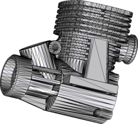
|
| Figure 1: Example of a 3D input boundary (represented with a mesh) where the quality of the triangles is very bad. |
Much effort has to be spent in order to generate a volume mesh of a complex geometry considering the existing meshing algorithms. Some of them are really fast and robust, but they require several geometry cleaning operations. If the time needed for them is added to the total meshing time, they became not so fast in practice. Contribute to reduce this extra effort is the motivation of this monography.
1.2 Objectives
The main objective of this monography is to develop an algorithm for isotropic unstructured volume mesh generation robust enough to be able to generate a mesh from non-cleaned input geometries, using as less input data as possible. This will lead to a drastic reduction of the time consumed in the pre-processing part, and will overcome the actual bottleneck in the whole simulation process.
The mesh generator must be flexible enough in terms of mesh adaptation to the solver requirements considering specific input data. The idea in this work is that the algorithm should be able to generate always a mesh from a given geometrical domain, almost without any specific meshing property assigned to it.
The meshing algorithm presented in this monography has been designed with the following objectives in mind:
- It should be prepared to use the more common geometrical definitions as input data reducing as much as possible its preparation (CAD cleaning operations).
- It must be able to run on a simple PC, but also it should be able to take profit from more complex computer architectures, which enable the use of parallel processing.
- It should be useful for a wide range of application fields. The main characteristics for the mesh to be generated are taken from the requirements for the FEM, but they are general enough to be applied to other numerical methods.
These characteristics lead to a set of requirements to be covered by the meshing algorithm developed in this monography. The main ones are: robust and fast mesh generation, and ability to mesh from non-watertight geometries. The explanation of all the requirements covered by the new mesher is detailed below in Sections 1.2.1, 1.2.2, and 1.2.3.
1.2.1 Mesher requirements
In this section, the requirements of the mesher developed in the monography regarding its behavior are detailed:
- Robustness. This is one of the key objectives and it can also be seen as a requirement for the input data, as this robustness refers to the capability of generating the mesh independently from the input data quality. Some of the existing unstructured volume meshers accomplish all (or almost all) the requirements presented in this work, but they require a very specific tuning of their parameters for successfully generating the mesh. Independently of the sizes assigned by the user, the quality of the input geometrical data or the general parameters chosen, the mesher should be able to generate always a mesh suitable for the simulation. The idea of the new algorithm developed in this monography is that it should generate always a mesh accomplishing the requirements defined in this section without a special training in the use of the mesher.
- Fast mesh generation. One of the key motivations of this work is to reduce the time consumed in the pre-processing operations for a numerical simulation. For this purpose the mesher has to be fast. Moroves, it has to be naturally fast, in the sense that it should imply fast and simple operations. Furthermore, its implementation should take profit from parallel computing strategies.
- Prepared to generate really large meshes. As the computer technology is evolving very fast, each time the solvers are capable to solve larger and larger algebraic systems. Thinking about the requirements from different simulations fields for the next years, the mesher should be able to generate billions of tetrahedral elements without problems. This characteristic is really important when deciding some implementation aspects of the algorithm.
1.2.2 Input data requirements
This section focuses on the requirements to be covered by the mesher concerning the input data:
- Accept non-cleaned input geometry. This is another key point of the mesher. The idea is that it should be able to generate the mesh of the model although its geometrical contour comes from a non-cleaned input geometry. In this context, a non-cleaned input geometry is defined as the one containing:
- Non-watertight volumes. This means volumes with contours presenting gaps or overlapping entities.
- Non-coherently oriented contour entities. This means that the contour entities of a volume are not needed to be oriented (all of them) towards the same part of the volume (inner or outer).
- Low quality definition. The geometrical contour can be defined by geometrical entities (like NURBS) or by a surface mesh. In this context, a geometrical contour with low quality definition means a highly distorted parametrization of the surfaces (in case of geometrical representation), or a mesh containing low quality elements (in case of surface mesh representation). Examples of low quality input geometries and no water-tight domains are shown in Figures 1 and 2. It has to be noted that the algorithm proposed in this document is for 3D volume meshing. However, for sake of simplicity, 2D examples are shown in some figures.
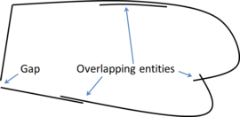
|
| Figure 2: Example of a 2D non watertight input boundary with gaps and overlapping entities. |
- Accept input data in geometry and mesh format. The natural input for a mesher is the geometrical definition of the contours of the model. This geometrical definition can be represented in several ways, but the most common ones are CAD or mesh entities. In this document, when talking about CAD entities, the NURBS surfaces and curves [4] (trimmed or not) will be considered, as they are the most general mathematical representation able to represent all the geometrical shapes.
Although the mesher should generate a mesh from a non-cleaned input geometry, some minimum criteria concerning topology or shape definition may be needed.
While mesh entities are simpler to be defined, CAD entities are a more precise way of defining a geometry. Meshes often loose continuity in the geometrical definition depending on the smoothness or curvature of the shape to be represented. It also has to be considered that, almost always, the mesh presents a chordal error compared to the smooth original geometry (the chordal error is the distance between a point on the mesh and the original smooth shape the mesh is trying to represent). In the Figure 3 a graphical representation of this chordal error is shown.
The simpler definition and treatment of mesh entities has made them the most common used as input for the existing volume meshers. There are cases where a surface (or a line) cannot be meshed because of its bad parametrization. In these cases, a volume mesher requiring a mesh as input cannot be used. This is the reason why the proposed volume meshing algorithm should be prepared to get as input data mesh entities, as well as NURBS surfaces and curves. Actually, it should be prepared not only to get these kinds of entities as an input, but also to work with them in the geometrical operations needed during the whole meshing process. The methodology presented in this monography is prepared to work either with CAD and mesh entities. Hence, the general form of geometrical entities will be used to refer the input entities defining the contours of the domain. Only if some specific operation is needed for just one of the representations it will be specified if the geometrical entity is a CAD or a mesh one. Following this duality, in this document a single term will be used to refer the different natures of geometrical entities:
- Surface entities for surface mesh elements (especially triangles) and geometrical surfaces (especially NURBS surfaces and patches of connected NURBS surfaces).
- Line entities for line mesh elements and geometrical curves (especially NURBS lines and groups of connected NURBS lines).
- Point entities for nodes of a mesh and geometrical points.
1.2.3 Final mesh requirements
The requirements to be covered by the mesher regarding the final mesh generated are:
- Maintain volume topology. The topology of the initial domain to be meshed must be preserved in the final mesh. For most meshing algorithms this requirement is automatically satisfied, but it is not automatically guaranteed in all meshing techniques. Considering the final mesh, it has to be possible to identify the volume each tetrahedron belongs to. Then, if getting all the tetrahedra belonging to a given volume, the concept of the mesh of that volume can be defined. The maintenance of the volume topology of the initial domain means that there must be a mesh for each of the initial volumes, and each volume mesh must represent the same relationship between the others. For instance, if two volumes are connected by a line, the meshes of these two volumes must be neighbors sharing line elements. Furthermore, the mesh of a volume itself must represent the topology of the volume (for instance, if the volume has a hole, the mesh must have a hole). In Figure 4 two examples are shown with meshes preserving or not the topology of the original model.
A special case which evidences the importance of maintaining the initial topology is the situation where the domain has very thin parts representing relevant details of it. A 2D case of this kind is shown in Figure 5, where a thin channel-like part can be identified in a surface (Figure 5(a)). Independently on the mesh desired size required by the simulation, the mesher must generate elements small enough not to close this channel-like zone, as the mesh shown in Figure 5(b). The mesh depicted in Figure 5(c) is not acceptable, as it does not preserve the topology of the domain.
| ||||||
| Figure 5: Example of surface mesh preserving or not the topology of the initial domain. (a) 2D geometrical domain formed by two surfaces (colored as blue and gray). (b) Mesh of the surfaces preserving the topology of the initial domain. (c) Mesh of the surfaces not preserving the topology of the initial domain. |
- Maintain a representative lines and surfaces topology. Often it is not required to preserve the topology of all the surface and line entities of the domain to be meshed. As the proposed algorithm is a volume mesher, the surface or line elements in the final mesh are of interest just in order to assign properties to them for the simulation. These properties can be of different nature: material properties, boundary conditions, etc. At the end, the mesher should maintain the topology of some patches of lines and surfaces on user demand, or following some automatic criteria.
Note that this requirement is not as hard as the typical constrained condition in the boundaries of the domain. Especially when the input data for a mesher is a surface mesh, it is common to require the mesher to be constrained at the boundary. This means that the contour mesh of the final tetrahedral mesh (the triangles representing the skin of the generated tetrahedra) must be topologically identical to the input surface mesh defining the contours of the domain.
| ||||||
| Figure 6: (a) Contour mesh of a volume with a set of triangles highlighted in red representing the region . (b) A partially constrained tetrahedra mesh generated from the contour mesh shown in (a) where the highlighted set of tetrahedra faces corresponds to the region . (c) A not constrained tetrahedra mesh of the contour mesh shown in (a) (it cannot be identified a set of tetrahedra faces representing the region ). |
In Figure 6(a) an example of the contour of a volume is shown, where a set of surface entities (in this case triangles)are colored in red. Let us call the region represented by those triangles. If the simulation requires a set of triangles representing the region , the mesh generator should provide with a tetrahedral mesh whose skin should have a set of triangles representing that region, but it is not needed for those triangles to be identical as the ones in the input geometry. A tetrahedral mesh accomplishing this criterion is shown in Figure 6(b). A totally unconstrained mesh is depicted in Figure 6(c), where it cannot be identified a set of triangles corresponding to the region . It is obvious that the mesh in Figure 6(b) is not constrained with the input boundary shown in Figure 6(a), as the triangles representing the region are different. However, it can be seen that the requirement of maintaining a representative topology of the surface and line entities of the input data allows a bijective relationship between groups of surface and line entities in the input data and surface and line mesh elements in the final mesh. This requirement is enough to allow an automatic assignment of data from the input boundary geometry to the final mesh entities.
- Generate automatically the contour mesh of the volumes. Although the mesher is thought to generate volume elements (tetrahedra), it should give as an output also the triangular elements corresponding to the contours of the volumes, and the line elements corresponding to the boundaries of certain patches of triangles. This surface and line elements correspond to faces and edges of the final tetrahedral mesh.
- Preserve geometrical features. This is automatically achieved by the boundary constrained meshers, but it is not guaranteed at all by the types of meshers. This requirement is crucial for the final mesh to represent the shape of the domain precisely. For several kinds of numerical simulations, the presence of sharp edges and corners in the domain affects drastically the results, as they often govern the physical behavior of the process to be simulated. The importance of preserving sharp edges and corners to represent some domains can be appreciated in Figure 7. Part of the contours of a volume are shown in Figure 7(a). The tetrahedral mesh of that volume generated without preserving the sharp edges of the input geometry is shown in Figure 7(b).
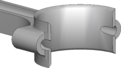
|
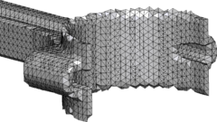
|
| (a) | (b) |
| Figure 7: (a) View of a part of the contours of a mechanical piece. (b) Tetrahedral mesh of the mechanical part generated without preserving the sharp edges of the input geometry. | |
In terms of the mesher, this requirement means that it should be partially constrained to some line entities from the input geometrical data, and must include fixed nodes in the final mesh (corresponding to specific point entities in the input data). In this context, partially constrained means that if some specific line elements in the input geometrical data must be preserved, a collection of edges from the final mesh should follow the path of those line elements. This is not as restrictive as totally constrained condition.
As it will be explained later on (Section 3.1), the strategy to cover this requirement will be also useful to reach the requirement of maintaining a representative lines and surfaces topology.
- Allow to skip given details of the domain. This requirement is somehow complementary to the previous one. What it means is that the mesher must be not constrained in some regions. The definition of the geometrical domains includes often very thin or small entities in given parts. The reason for the size of these entities may be the size of the part of the domain represented itself, but the presence of these small entities often responds to the application of a given tangency criteria for the geometrical definition, or they are just the result of some geometrical operation previously done (intersections, Boolean operations, etc.). The basic idea of this requirement is that the sizes of the geometrical entities used to define the contours of the domain are not necessary related to the mesh size needed for the simulation. In the Figure 8, an example is shown where the triangles generated from a patch of surfaces skipping the inner lines between them are much larger than the size of some of the surfaces of the patch. Clearly the simulation should not need such thin triangles in the regions where the surfaces are so thin.
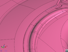
|
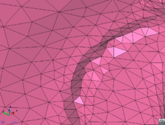
|
| (a) | (b) |
| Figure 8: (a) Zoom of a patch of surfaces representing a mechanical part. (b) Triangle mesh of the patch of surfaces shown in (a). | |
Even when the sizes of the input entities are related to the representative size of a specific shape to be represented, the user may desire a bigger mesh size to skip the representation of given details because they are not of interest for the simulation. Instead of forcing the user to modify the input geometry which defines the domain, this requirement makes the mesher skip the detail within the mesh generation process.
The accomplishment of this requirement will let the user to define a desired mesh size distribution in the final mesh just because of the simulation requirements, and not because of the initial way of defining the geometry. In terms of the mesher, this requirement means that it should be able to skip some of the line and point entities from the input geometrical definition of the domain. The entities to be skipped should be defined automatically following some given criterion, or by the user.
- Precise representation of the contour geometry. This requirement focuses on the need of the nodes of the contours of the final mesh to lay exactly on the geometrical entities defining the contours of the domain. Some mesh generators only approximate the shape of the domain to be meshed, or represent its contours in a staircase manner (specially the meshers based on octree or bin structures). Several numerical methods (specially the FEM) need a precise representation of the contour, as its shape and smoothness may affect drastically the result of the simulation. This is the main reason for this requirement.
- Final elements quality ensured. The acceptable quality of the mesh elements is a relative parameter, as the different methods used for the numerical simulation are applicable for different ranges of element qualities [5]. Usually, most numerical methods perform better as the shape of the element is closer to the corresponding regular polyhedron, however this cannot be extended to all numerical simulations. This requirement will try to reach a minimum dihedral angle in the final tetrahedra.
- Allow a 3D spatial size assignment. The use of a non-uniform mesh is crucial for some simulations. In some specific regions of the domain the size of the elements may have an upper bound, but if that size is used in the whole domain the final mesh should have too many elements. Typically, in the regions where there are higher gradients of the variable under study, the simulation needs a finer mesh than in other regions. This requirement is also important in the accurate representation of the shape of the domain, as the curvature of the domain geometry is strongly related with the mesh size needed to accomplish a given chordal error criteria. Just for geometrical purposes, a refined mesh in some regions would be needed.
- Control of sizes transitions. As the final mesh can be non-uniform size distributed, the size of the elements should vary from a region of the domain with a desired size to another. Some numerical simulations do not only require a specific mesh size in some specific zones, but also a given growing law between neighbor elements. The mesher should let the user to control how the element sizes grow (or decrease) from a region of the domain, depending on the distance from the elements to that region.
- Applicable for immersed methods. A family of methods for numerical simulations are the so-called immersed methods and embedded methods [6,7]. The main characteristic of these methods is that they do not require a body-fitted mesh to represent the domain. The shape is implicitly introduced by distance from the nodes to the boundaries and a casting process (determine whether a node is inside or outside the domain). In some sense, generating a mesh for a simulation using an immersed method is less restrictive as the geometrical features should not be preserved, but in contrast, the final mesh must have extra information attached. This information is the distance from each node of the mesh to the boundary of the domain.
1.2.4 Surface meshing
Although the main objectives of the monography are related to volume meshing, there is a secondary objective for the new mesher, which is to be able to mesh 3D surfaces and lines which are not boundary of any volume accomplishing the requirements defined above. This capability would give several advantages to the method:
- Generate conformal meshes of volumes containing inner surfaces or lines. These are entities totally inside the volume, but not belonging topologically to the boundaries of the volume. An example of this case could be the representation of a sail (3D surface) into a control volume in order to perform a CFD simulation. The sail is totally inner to the control volume, and the mesh of it must be conformal with the tetrahedra representing the control volume. A 2D example of this case is shown in Figure 9. In this example a surface (bounded by solid black lines) has an inner line (dotted black curve), and the mesh of the surface (in gray) is conformal with this line.
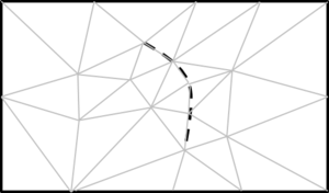
|
| Figure 9: 2D example of a surface mesh (gray lines) conformal with an inner line of the surface (dotted line). |
- Mesh in a conformal way a model with volumes and surfaces or lines connected to them. A case of two volumes connected by a surface is depicted in Figure 10. The mesh of the volumes and the surface must be conformal in the contact lines between them. This case can be also meshed by generating separately the volume meshes with the octree mesher, and afterwards mesh the surface using other meshing algorithms. This would not take profit on the advantages of meshing the whole model at once.
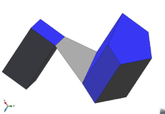
|
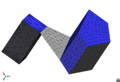
|
| (a) | (b) |
| Figure 10: (a) Example of a model containing two volumes (in blue) and a surface (in grey) connecting them. (b) A conformal mesh of the model considering the volumes and the surface mesh. | |
- Mesh patches of surface entities together preserving features, but skipping the inner line entities between them if needed. The entities to be skipped could be detected automatically following a given smoothness criteria, or under user demand. Figure 8 shows an example of triangle mesh representing a collection of surface entities, but skipping the inner line entities.
- If the patches of surfaces are not topologically connected, the proposed method could act as a CAD cleaning tool, as it could extract a continuous manifold surface mesh from a collection of surface entities with gaps or overlaps. The extraction of surface skin meshes from a volume discretization has been used in [8] and [9], and it is interesting for CAD cleaning, as well as for boolean operations involving non-watertight geometries. The preservation of geometrical features is essential for these purposes.
1.3 Structure of the monography
The monography is structured in the following chapters:
- Chapter 1: Introduction. This chapter focuses on introducing the context of the presented work. Its motivation is explained (Section 1.1), and its objectives are detailed (Section 1.2).
- Chapter 2: State of the art on mesh generation. In this chapter the different mesh types are presented (Section 2.1) as well as the state of the art of different meshing techniques (Sections 2.2, 2.3, 2.4 and 2.5). The advantages and drawbacks of each meshing method is studied, and the proposed solution for the meshing algorithm is justified (Section 2.6).
- Chapter 3: Basic concepts of the new mesher. Several concepts and some auxiliary algorithms are defined in order to allow a better understanding of the meshing algorithm presented. Its main parts are:
- Definition of the input data for the presented meshing algorithm and a proposal of how the mesher can interact with CAD data, integrated within a pre-processing system (Section 3.1).
- Octree structure characteristics (Sections 3.2 and 3.3). The definition and main characteristics of the octree structure (which plays a key role in the presented work) are presented. Special interest is given to its specific properties for the meshing process. The notation is defined which will be referred to in the following chapters.
- Geometrical intersections (Section 3.4). As the geometrical intersections are crucial for some of the algorithms presented, this section analyzes them deeply and studies the pathological configurations that may occur.
- Chapter 4: Coloring algorithm. The coloring process determines where a point in space is topologically: it determines if it is outside the domain, inside a given volume, or onto an interface between volumes. This is one of the main operations involved in the presented mesher and can be understood as an auxiliary algorithm for the meshing itself, so a whole chapter is devoted to it. In this chapter different approaches to solve the coloring problem are studied (Section 4.1), and a new algorithm based in the ray casting technique is exposed (Section 4.2). The implementation of this algorithm is presented in Section 4.3.
- Chapter 5: Octree based mesher. This chapter focuses on the new meshing algorithm itself. After an introduction, where its main idea is highlighted (Section 5.1), the algorithm for embedded (Section 5.2) and body-fitted (Section 5.3) meshes is detailed.
- Chapter 6: Implementation aspects. In this chapter all the implementation details for the meshing algorithm developed are explained. After some general aspects of the implementation (Section 6.1), the implementation of the octree structure is analyzed (Section 6.2). Sections 6.3, 6.4, and 6.5 focus on the implementation of specific parts of the meshing algorithm itself. Some considerations on the parallel implementation of the mesher are pointed out in Section 6.6. A list of the values of the parameters relevant for the mesher used in the presented implementation of the algorithm is detailed in Section 6.7.
- Chapter 7: Examples. In this chapter the results of some validation examples highlighting specific characteristics of the presented mesher are shown (Section 7.1). Sections 7.2 and 7.3 analyze the results of the meshing algorithm applied to real complex geometries under different configurations.
- Chapter 8: Conclusions and future research lines. This chapter lists the conclusions of the presented work (Section 8.1) and proposes some futures lines of research (Section 8.2).
- Appendix A: Profiling tables and complete data of examples. In this appendix, tables with all the profiling data concerning times and memory for the whole configurations used in the examples run to validate the meshing algorithm are provided.
It is highlighted that, although the meshing algorithms presented are directly applied to volume meshing, most of the geometrical operations are applicable (with slight modifications) to surface meshing in 2D cases. Taking into account that some concepts are much more clear to understand from a 2D scheme (especially when dealing with geometry), in this monography 2D examples are used sometimes to illustrate some of the concepts explained.
2 State of the art on mesh generation
In this monography isotropic volume meshers are considered. Isotropic meshers can be defined as the ones trying to generate elements as much regular as possible, understanding a regular element as the one whose edges have the same length.
2.1 Mesh types
There are two main families of meshers depending on the kind of mesh they generate: structured and unstructured [10]. Actually, a third kind of meshers can be classified as semi-structured ones. A structured mesh is defined as a mesh which all inner nodes have the same degree (the degree of a node is the number of elements owning it), while the nodes of an unstructured mesh have different degrees. Semi-structured meshes can only be applied to topologically prismatic geometries, and they basically repeat the structure of an unstructured mesh (in the tops of the prismatic shape) in different layers following the structured direction. An example of this kinds of mesh is shown in Figure 11.
Unstructured meshers [11,5,12] can be divided in three main families: advancing front, Delaunay and space decomposition methods.
In the following sections, the main characteristics of these methods as well as their main advantages and drawbacks are detailed, focusing on the requirements defined in section 1.2. The aim of this chapter is to highlight which of those requirements are covered by each meshing method, so the algorithms are not deeply detailed and only their main characteristics are pointed out.
| ||||||
| Figure 11: Examples of different types of mesh(a) Structured triangle mesh. (b) Unstructured triangle mesh. (b) Semi-structured prism mesh. |
2.2 Structured meshers
Structured and semi-structured meshers often get as input data the position of the nodes in the contours of the domain, and generate the inner nodes positions from a given interpolation [10,12,4]. The quality of the final mesh obtained is directly related to the kind of interpolation used and the degree of distortion of the contours of the domain, so a minimum level of element quality cannot be guaranteed for arbitrary domains. However, for good shaped volumes and uniform sizes distributions these methods provide with very good quality meshes.
The main advantages of structured meshers are:
- Fast and robust. As they are based on a given predefined interpolation, they are really fast and robust.
- Parallelizable. Apart from being fast, these kind of meshers are very parallelizable.
On the other hand, these meshers have some important drawbacks:
- Need of specific topology for the input data. The main problem of this kind of meshers remains in a requirement for the input data: they need a specific topology for the geometrical definition of the contours of the domain. As an example, to generate a structured mesh of hexahedra, the input geometry must be topologically an hexahedra. This means it has to be a volume with 6 contour surfaces, and each one of their must have 4 contour lines. This requirement makes impossible to use this kind of meshers for arbitrary geometries with complex topology. A family of methods has been proposed that are able to skip this problem [13]. They are basically based in decomposing the original domain to be meshed into different parts which do accomplish with the topology demanded by the mesher. Then, each of these parts can be meshed in a structured manner, so they are often referred as structured by blocks or multi-block meshers. Several implementations of these methods have been carried out [11,10], but in practice they are meaningful for very specific domains only. Depending on the topology required by the mesher, some geometries are impossible to be decomposed in such this way, and even when this decomposition is possible, from complex original geometries is not obvious to generate this decomposition automatically. This often implies an extra pre-processing operation before using the mesher, which is the splitting (manually) of the domain in different parts.
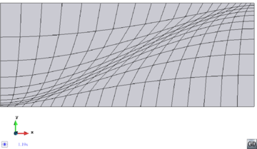
|
| Figure 12: Example of a 2D structured quadrilateral mesh with a non-uniform size distribution. A high level of element distortion can be appreciated. |
- High distortion in non-uniform meshes. As the nodes of structured meshes have the same degree, a predefined topology of the mesh is forced. It generally tends to generate uniform meshes. Structured meshers can relatively distort the elements in some region in order to provide with a non-uniform mesh, but the fixed topology of the mesh does not allow a sharp sizes transition without an excessive distortion in the elements. A 2D example illustrating this problem is depicted in Figure 12.
2.3 Advancing front method
The advancing front method [14,15,16,17] is a common technique for generating unstructured meshes. It gets a closed and oriented mesh of the boundary of the domain as input and mesh its inner part. The surface elements of this mesh are the ones in the active front, and the algorithm can be summarized with the following points:
- From each element in the front (face) a new volume element is generated. An optimal position of the node needed to build the element is obtained and the nodes and faces of the active front close to it are considered. The new element is build using a new node in the optimal position or an existing close node, depending on the resulting configuration: the new element should not intersect any one of the close already existing faces.
- The active front is updated adding the new faces created, and removing the ones already shared by two elements.
- These two steps are repeated until there are no faces in the active front. Then all the domain has been filled with volume elements.
Although the advancing front is mainly used for generation of tetrahedral (or triangle in 2D) elements, some adaptations of the method have been done to generate other types of elements [18], and even for generating particles for DEM simulations [19]. The present work is focused in tetrahedra mesh generation. There are several possible implementations of the advancing front method [11] depending on the way of creating the new elements from a face of the front, the way of considering the mesh desired size in the inner part of the domain, or the order in which the faces of the front are processed, among others. In special, much work have been done in order to improve the efficiency in evaluating the desired mesh size in a specific region of the domain, and control a smooth size transition in the final mesh. This is one of the strong points of advancing front techniques, as the creation of each element can fit very well the desired mesh requirements. Different approaches use a background grid to set the mesh desired size [16,15,20,21], or sources from which the desired mesh size vary following a given function [22], which provides with a very smooth transition between element sizes. A combination of different methods can be used in order to improve accuracy and reach an efficient implementation of the method [23]. However, independent of the implementation, one can identify some general advantages and disadvantages of advancing front based techniques. The main advantages are:
- Good quality meshes. In the advancing front method, each new element is created connecting a face of the active front with a new node or an existing one. This choice is done based on an optimal position for this new node in order to get the best element (in terms of quality) taking into account the desired size of the mesh in that region. This methodology for creating the elements gives high quality elements in the final mesh, even before any smoothing process.
- Automatic preservation of topology. The advancing front method is naturally constrained, as each element of the surface mesh of the contours of the domain to be meshed will become a face of the final tetrahedra.
- Good control on the size transitions. As explained before, each new element is created from an existing face and an optimal position of the node to create the element from the face. Considering the desired size for the final mesh in the region where the face is, and the size of the face itself, the size transitions from one part of the mesh to another is totally controlled.
- Parallelizable. The creation of each new element using the advancing front method is clearly local. The geometrical and topological checks needed to create the new element only take into account the nodes and faces inside a specific radius of influence of the face the new element is created from. This aspect makes totally independent the creation of an element from the creation of another element which is far enough. Although it is not obvious to implement an efficient parallel version of the advancing front method, at least the element generation method is local enough to make the implementation affordable. [24] proposed a first octree subdivision of the domain, and then apply the advancing front technique in each of the cells of the octree, seaming afterwards the interface parts between cells.
The main drawbacks of the advancing front method are:
- Strong dependency on the contour mesh quality. Considering that the surface elements of the initial contour mesh will be faces of the final volume elements, the quality of these contour elements is totally related with the quality of the tetrahedra in contact with them: if a triangle of the contour of the domain has a very small angle in some of its nodes, the resulting tetrahedron from it will have a very small dihedral angle. This implies a great effort in the mesh generation of the contours of the volumes to be meshed. Often this effort takes most of the part of time in the pre-processing operations of the whole simulation when using the advancing front technique.
- Requires watertight input geometry. The reason for this is that the initial surface mesh representing the boundary of the domain will be the skin of the tetrahedra in the final mesh.
- Not very robust. Theoretically, the advancing front is a robust method. However, the locality of the element creation process and the checks needed to evaluate if the new element created intersects or not the active front require some tolerances. These tolerances must be tuned precisely in order not only to avoid the crossing of the active front, but also to avoid different parts of the front to get very close. This situation can lead to geometrical configurations of the active front which make almost impossible the creation of a new element. The tuning of these tolerances and other parameters can be done as general as possible, but as the active front evolves during the meshing process, these geometrical configurations are not under control, and cannot be predicted. This aspect, together with the hard dependency on the contour mesh quality makes the advancing front method not so robust in practice.
- Not very fast. Every candidate new element to be created needs to be checked in order to verify if the active front is intersected by some of its faces and edges. This involves the use of several geometrical intersections operations in the whole meshing process. This aspect, together with other characteristics of the advancing front method, makes it not very fast in comparison with other meshing algorithms.
2.4 Delaunay method
A Delaunay mesh is defined as a mesh which elements accomplish the Delaunay condition: the circumcircle (in 2D case) or the circumscribed sphere (in 3D case) of any element has no node from the mesh inside [10]. Given a cloud of points, a Delaunay triangulation can always be created from their Dirichlet tesselation connecting them with a set of triangles (in 2D) or tetrahedra (in 3D) without adding any extra node [10].
The Delaunay meshing methods [12,25,5,11] depart from the contour of the domain and generate the Delaunay triangulation of its nodes. This mesh is the convex hull of the domain to be meshed. Although it is already a mesh, its elements may have a low quality, or may not fit with the desired mesh size in that region of the domain: these are the bad elements. The following strategy is applied recursively to all the bad elements:
- A node is created in the centroid of the element. Some strategies allow the creation of the new node at the edges or faces of the elements [26] in order to improve the quality of the elements respecting the contours of the domain.
- All the elements of the mesh which circumscribed sphere (or circumcircle in 2D) includes the new node are deleted. Note that a void region is created containing the new node inside.
- A Delaunay triangulation is created with the new node and the contour nodes of this void region.
This procedure leads to a Delaunay mesh (accomplishing the Delaunay condition), but this does not guarantee a given level of quality by itself. Often, some elements can present very low quality (especially in 3D cases). These elements may have null volume and are called slivers. Even if its volume is equal to zero, they can accomplish the Delaunay condition. For this reason, it is common to relax the Delaunay condition in some regions in order to avoid quality problems [27].
The main advantages of this method are:
- Robust. Mathematically, we can always obtain a Delaunay mesh from a cloud of points. However, sometimes the modifications of the method to cover the requirements of the simulation make it not so robust.
- Fast. Although it depends strongly on the implementation, it can be said that Delaunay methods are naturally faster than the advancing front ones.
The main drawbacks of the Delaunay method are:
- Naturally not constrained. Delaunay methods use the representation of the contour of the domain as an initial configuration for the insertion of nodes procedure, but the final mesh boundaries are not guaranteed to be constrained with that contour. Some strategies can be applied [28,29,30] in order to guarantee that the nodes in the initial contours will lay on the contour of the final mesh, or even a constrained condition in the faces of the initial contour, but these modifications reduce the performance and robustness of the method. Furthermore, if there are huge different mesh desired sizes in the domain, these strategies are not very robust.
- Requires watertight input geometry. As in the advancing front method, the contours of the domain are required to be watertight. Actually, a strategy could be followed to treat non-watertight geometries. It is based on generating the first mesh (the convex hull in the traditional Delaunay methods) using only the nodes of the contours, with an automatic recognition of the boundaries: the so called alpha-shape method [31]. This would indeed generate a volume mesh from a non-watertight geometry, but there is no enough control in the boundaries recognition to ensure that mesh correctly represents the topology of the domain.
- Not naturally parallelizable. The check of the Delaunay condition of an element requires taking into account all the mesh entities participating in the circumscribed sphere of the element. As its radius depends on the position of the nodes of the element (cannot be bounded a priori), the treatment of one element can involve the whole mesh in some configurations. This implies a hard dependency ranging from an element to the whole mesh, so a parallel implementation of the method is not obvious. However, some parallel implementations (mainly for shared memory paradigm) of the Delaunay method have been carried out, [32] or [33].
2.5 Space decomposition methods
Space decomposition-based methods follow a different philosophy than the methods explained before. To generate the mesh, they basically subdivide the space into cells providing with a spacial decomposition covering the space where the domain is (overlapping the domain). These cells can be thought in a general way, but it is common to use one of the following main structures which govern their configuration:
- Bin: a bin structure provides with an homogeneous grid as the space decomposition formed by regular cells (squares in 2D or cubes in 3D). A graphical view of a 2D bin is shown in Figure 13(a).
- Octree: an octree (quadtree for the 2D case) is basically a hierarchical spatial structure that partitions the 3D space into regular cells [34]. These cells can be refined in given zones of the domain. A graphical view of a quadtree is shown in Figure 13(b). A more detailed definition of the octree structure is given in Section 3.2.
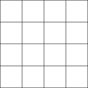
|
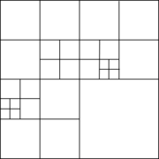
|
| (a) | (b) |
| Figure 13: 2D examples of typical structures used in space decomposition based meshing algorithms. (a) Bin. (b) Quadtree. | |
The bin structure is suitable for homogeneous discretizations. It is common to use an octree structure as the regular grid (which gives the name of the family of methods), because it is more flexible for mesh generation purposes, as domains to be meshed and desired mesh sizes are commonly non-homogeneous. Octree-based meshers were pioneered by Yerry and Shephard in [35] and, since then, several approaches have been proposed [36,37,38,39,40,41,42].
The octree structure was thought for the first time for space searching purposes [34], and the specific topology of the spatial decomposition it represents (detailed in Section 3.2) gives several advantages for mesh generation. Somehow, an octree can be considered a mesh itself (it can be thought as a non-conformal hexahedra mesh), so it is really natural to build a mesh from it.
Although several algorithms have been proposed parting from the octree-based family of methods, almost all of them follow three main steps:
- Generate the regular grid for the space decomposition.
- Generate the elements of the final mesh directly using given patterns from the cells of the regular grid.
- Fit somehow the boundaries of the domain.
Concerning the first step, as it has been pointed out before, the octree is the most common structure used for the space decomposition. From the theoretical point of view, all octrees are similar, but depending on the way the octree will be used, different implementations have been proposed by several authors [43,34] in order to improve the efficiency of the octree, the performance for searching processes, the optimization considering the memory needed to store it, etc... More details on the implementation of the octree are presented in Section 6.2.
The generation of the elements of the final mesh from the octree is a simple process. It is based in creating the mesh elements directly from the octree cells (the definition of octree cell, as well as other octree related basic concepts are explained in detail in Section 3.2). Some of the existing methods apply different splitting patterns from the cells to get tetrahedra [35,44,37]. Other methods can get directly the cells of the octree as hexahedra elements of the final mesh (in cases where the final mesh is not needed to be conformal), or create transition elements when two neighbors present hanging nodes [42]. [40] proposes a different approach: create special cells where the octree is refined (where the neighbor elements are not conformal) and build the dual of the octree. The cells of it are directly the elements of the final mesh. With this approach a final mesh of conformal hexahedra is obtained automatically.
The key difference of each method remains in the third step, which is the most complex one. As the octree is a regular space decomposition, their cells do not fit exactly the contours of the domain to be meshed. Getting only the elements coming from the cells which are in the inner part of the domain (or even the ones intersecting its boundaries), the contours of the final mesh are staircase-like, so they are not able to represent smooth shapes with a given curvature.
Considering the inner cells (the ones totally inside a volume) and the interface ones (the ones colliding with the contours of a volume), different strategies have been proposed to fit the contours:
- Get only the inner cells and fill somehow the empty space between them and the real contour of the domain. This family of methods profits from the main advantages of octree-based methods for the inner part of the domains, but presents the same limitations near the contours as the methods used to fill those empty spaces.
- Project onto the contour of the domain the boundary nodes of the elements created from the inner cells using different techniques [36,39]. This strategy warps the nodes coming from the octree, so the shape of the octree changes, but its topology remains the same. [42] proposes a pillowing technique near the contours to avoid bad shaped elements (hexahedra) after mapping the nodes.
- Move some nodes and split the elements intersecting the contours of the domain in order to represent it precisely [37].
Although these methods achieve the smooth representation of the contours, they have to follow specific strategies to preserve the geometrical features (corners or sharp edges). [41] proposes a re-tetrahedralization of the octants of the octree containing sharp edges using advancing front or Delaunay technique, taking into account the intersection points between the sharp edges and the octree cells. [40] follows a strategy based on detecting which triangle from the input boundary the final nodes lay onto, and assuming that if two nodes lie onto two triangles connected by a sharp edge, there should be a sharp edge between those nodes of the final mesh. This strategy is not so robust, as it assumes that the sizes of the final elements is quite similar to the sizes of the triangles of the contour, so the triangles where two neighbor nodes of the final mesh lie onto are supposed to be neighbors connected by an edge. This is not a general situation.
As it has been explained, several approaches have been proposed departing from the octree-based family of methods. Although each approach has its own characteristics, some common advantages can be detected:
- Robust. The operations involved in most common octree-based methods are designed to be robust independently on the tuning of their control parameters. This is applicable to the operations dealing with the octree itself, but some processes dealing with the mesh generated (especially for body-fitted meshes) may not be so robust.
- Fast. As mentioned above, the octree is a structure used to make faster the searching algorithms in space. Indeed, almost all the meshing algorithms use an octree as a tool for searching purposes. In this case, this structure is also the base of the mesh generation itself, so the algorithm takes profit from it to improve its performance. Furthermore, the inner elements of the mesh are created directly based on a division pattern of the octree cells, which is really fast in comparison with other methods which have to take care on geometrical aspects when generating each element.
- Naturally parallelizable. The octree itself is a partition of the space, so it is really easy to identify the parts of the domain affected when some part of the mesh is modified or generated. Furthermore, typical operations involved in an octree-based mesher are performed at octree cell level, and most of them are independent from one cell to another, so the parallelization of some parts of the algorithm is almost automatic. Several parallel implementations of the octree structure have been carried out taking advantage on these features [TU:2005:SPO:1105760.1105769,CamataCoutinho].
- Good quality meshes. As the mesh elements in these methods come from a predefined pattern of decomposition of an octree cell, all the inner elements are in a range of qualities known a priori. However, the elements in the contour of the domain are typically more distorted (depending on the method used).
- Allow not cleaned geometry as input. Most octree-based methods only take care on the position in space of the boundaries of the domain rather than a topological relationship between the contour entities. This is a key point to allow some of the octree-based meshers to work with non-watertight input geometries. This property also makes octree-based meshers independent from the quality of the contour meshes used as input.
The main drawbacks of octree-based methods are:
- Naturally not constrained. The space decomposition of the octree does not respect the topology of the model. Octree-based methods are often not constrained, and the topology preservation is usually linked to the sizes of the octree cells used. This ends with a need for the user of the mesher to assign properly the desired sizes of the mesh, taking into account some kind of characteristic size of the model in specific regions of the domain.
- Hard to preserve geometric features. This drawback is strongly linked with the previous one: as the mesher is not constrained, it is hard to preserve sharp edges or corner points from the input data in the final mesh. Furthermore, cases where the sharp edges involve a small dihedral angle are very unfavorable for these methods, as the octree cells are very regular by its nature: it is hard to represent a small angle parting from a regular shape.
- Predefined size transitions. As most elements come from a direct pattern from the octree cells, the size of an element in comparison with the size of its neighbor is strongly related with the sizes ratio between neighbor cells in the octree. This link makes quite stiff the possibility of applying a smooth size transition in the final mesh. For some simulation methods, the meshes obtained by octree-based meshers present (locally) too sharp variations in the sizes of neighbor elements.
- Alignment of edges in a preferred direction. Because of the regular partition of space the elements come from, these meshes tend to generate meshes aligned with it. This alignment may influence the solution of the numerical simulation depending on the method used.
- Creation of too refined meshes. Octree-based meshers tend to generate a large number of elements, specially when the model has sharp features. This is because these methods often try to guarantee a minimum element quality by refining the octree near them.
2.6 Proposed solution
The strategy chosen in this work to cover all the requirements described in Section 1.2 is to develop an octree-based mesher. The election of an octree-based mesher in this work has been made taking into account the main advantages and disadvantages of the different methods:
- Structured and semi-structured meshers have been disregarded because the requirement for the input geometry to present a given topology is so restrictive that it makes them non applicable for many complex cases.
- Advancing front like methods have not been taken into account because the hard dependency they have on the quality of the input mesh for being successful in the mesh generation. Furthermore, they are directly not applicable if the input geometry is not watertight, unless some geometry repairing process is applied prior to the meshing itself.
- Delaunay methods have not been taken into account because they are not naturally constrained, and the proposals for them to be constrained blur some of its advantages. Furthermore, Delaunay methods are not naturally parallelizable, and they often generate localized bad quality elements.
- Octree-based methods are fast, robust and lead to very good quality meshes. Their main disadvantage are the inability to preserve the input topology, and their not constrained nature. However, the advantages of this family of methods, together with the ideas presented in this monography to overcome these drawbacks have tipped the balance to these methods.
As explained in Section 1.2.4, although the main objective of this work is to develop a new volume mesher, the methodology proposed is applicable to generate meshes of 3D surfaces and lines not belonging to any volume. The case of lines is automatically solved with the special treatment of line elements in the volume mesher (Section 5.3.1), and some adaptations are maid to the volume mesher in order to mesh surfaces as it is explained on Section 5.3.10.
3 Basic concepts of the new mesher
This chapter focuses on defining the different concepts involved in the proposed meshing algorithm, as well as some auxiliary algorithms needed to understand it. The following concepts will be described:
- Input data (Section 3.1). The input data needed for the mesher is defined, as well as the way of interaction of the mesher with a CAD system.
- Octree structure (Section 3.2). As the octree is the base structure for the mesher, an introduction to it is carried out in this section, highlighting its main characteristics.
- Octree properties for mesh generation (Section 3.3). Some specific properties of the octree are used in the meshing algorithm. A detailed explanation of them, as well as the key notation is introduced.
- Geometrical intersections (Section 3.4). The way the new algorithm deals with the geometrical intersections is presented. Also, the notation of pathological intersection types is introduced. This issues will be referred to in other parts of the work.
3.1 Definition of input data
The essential input for the mesher is the geometrical definition of the boundaries of each volume of the domain. As indicated in Section 1.2.2, this definition can be carried out using CAD or mesh entities. In this document the general concepts of surface, line and point entities will be used for both representations.
At this point, it has to be commented that the mesher considers the outer part of the domain as another volume to be meshed. It takes the name of outer volume, or volume number zero. Of course, the outer volume extends until infinite and it has no sense to consider it as a closed volume, so it is treated in a special manner. Later on it will be explained in more detail how the mesher deals with it.
Together with the surface entities an extra information is needed: the identification of the volumes each surface entity is interfacing. Note that considering the outer part of the domain as a virtual volume, all the surface entities defining the domain are interfacing two volumes. It may have sense for a surface entity to interface more than two volumes, but this would imply overlapping definitions of the 3D space (parts of space belonging to more than one volume). These kinds of topology are not considered in the present work.
Apart from the geometrical definition of the boundaries of each volume of the domain, extra information can be given to the mesher in order to specify some characteristics of the final mesh. It is important to note that this extra information is optional, as the mesher should generate the mesh of the domain with or without it. This information is given by the mesh size entities, the forced point entities, the forced line entities and the general parameters. Hereafter the characteristics of these data are detailed:
- Mesh size entities. The mesh size entities are geometrical entities used to provide the mesher with the desired size of the mesh in different regions of the 3D space. These geometrical entities can be point, line, surface or volume entities (both in mesh or CAD form), and they have a desired mesh size associated to them. These entities can be part of the input boundaries or not. If a desired mesh size is needed to be assigned to a volume, it can be provided just with the identification of the volume, without the need of creating the corresponding geometrical entities (volume entities in this case).
- Forced point entities. These are positions in space where the final mesh is forced to have nodes. They can be part of the input boundaries or not.
- Forced line entities. These are line entities to be preserved in the final mesh. This means that the final tetrahedra mesh will have a connected path of edges identifiable as a linear mesh of each forced line entity. As an example, the line entities in Figure 14(a) can be considered as forced line entities, as a path of connected edges representing it can be identified in the mesh shown in Figure 14(b). Forced line entities can be part of the input boundaries or not.

|

|
| (a) | (b) |
| Figure 14: (a) Contours of a volume highlighting some of its forced line entities. (b) View of the tetrahedra mesh of the volume highlighting the sharp edges corresponding to the forced line entities in (a). | |
- General parameters. These are some global parameters which govern the behavior of the mesher and are not attached to geometrical entities. These parameters are optional, as the mesher should work without them, but they can help to fit the final mesh into the requirements of the simulation. Hereafter there is a list of these parameters:
- General mesh size. This is the mesh size desired in the regions of the domain where there are no mesh size entities. If this parameter is not entered, the general mesh size is taken as the size of the bounding box of the domain.
- Size transition factor. It controls the behavior of the size transition function. The definition and use of this function is explained in Section 5.2.2, and it basically determines if the size of the elements grows faster or slower from the areas where the mesh size is smaller to the ones where it is larger.
- Maximum angle for sharp edges. This is the dihedral angle below which an edge of the input geometry is considered to be preserved in the final mesh.
- Maximum chordal error. Two values may be needed: a relative and an absolute limit for the chordal error allowed for the mesh to be generated.
- Maximum distance between overlapping boundaries. This parameter is named . It is only applicable in case of non watertight geometries. It represents an estimation of the maximum distance between overlapping surfaces interfacing the same volumes. The definition and use of this parameter is explained in Section 3.4.
Apart from all these data, extra information can be attached to the entities defining the input boundaries: the external data. The external data can be of any nature and it has no relevance for the meshing process, but the mesher will transfer it to the corresponding entities of the final mesh. As an example, if a surface entity defining part of the boundary of a volume has some external information, the nodes of the final mesh placed on that surface entity, or the faces of the tetrahedra with all its nodes onto it will have the same external data attached to them.
3.1.1 Integration with CAD data
To prepare all the data needed for a numerical simulation it is common to use a software tool: the pre-processor. As explained in Chapter 1, part of these data is the mesh representing the geometry of the domain. As the geometry of the domain is often provided in a CAD format, pre-processors typically are forced to work with CAD data and generate the meshes for the simulation. This is the reason why pre-processors are often CAD systems, and they include several meshers inside.
From the point of view of a general pre-processor or a CAD system willing to use the presented mesher, there are some interesting aspects to be considered. Typically the geometrical entities inside these systems have several information attached related with the simulation data (boundary conditions, material properties, etc...) or to the CAD system structures (layers grouping the entities, topological information, etc...). This information must be transferred to the generated mesh, which implies the following requirement for the mesher: it should return specific meshes representing given geometrical entities (not only volumes, but also curves and surfaces).
The mesher should provide not only with the tetrahedra generated, but also with triangular meshes (made of triangles which are faces of the tetrahedra) and linear meshes (made of linear elements which are edges of the tetrahedra). Actually point entities can also be identified with a final node in the mesh, just by setting the corresponding point entity as a forced point entity.
The way to make the mesher returns (apart from the tetrahedra meshes of the volumes of the domain) the mesh of some line or surface entities from the input data is explained hereafter.
How to get the mesh of a line entity:
- Set the line entity as a forced line entity in the input data.
- Assign a specific external data to the line entity.
- The mesher will return a set of linear elements with the same external data attached.
How to get the mesh of a surface entity:
- Considering the line entities which are contour of the surface entity, set them as forced line entities in the input data. Note that the contour line entities of a surface entity form a closed path of line entities (actually, more than one set of closed paths can be present when the surface entity has holes).
- Assign a specific external data to the surface entity.
- The mesher will return a set of triangular elements enclosed by the forced line entities with the same external data attached. This situation can be seen in Figure 6: the patch of triangles in Figure 6(c) is the surface mesh of the surface entity represented by the highlighted triangles in Figure 6(a) (region ). To achieve this situation, the line entities surrounding the region should be set as forced line entities.
Following this mechanism, the pre-processor can obtain not only the mesh of the volumes of the domain, but also the mesh of any line or surface entity. Once a mesh of an entity can be identified, all the information of the input entity can be transferred to the corresponding part of the final mesh.
3.2 Octree structure
As the octree is a key structure in the proposed mesher, a brief introduction is given in this section to highlight its characteristics.
| ||||||
| Figure 15: Example of a quadtree structure. (a) The root cell of a quadtree. (b) Root cell subdivided in 4 cells. (c) Example of a quadtree refined 4 levels. |
An octree (quadtree in the 2D case) is basically a hierarchical spatial structure that partitions the space [34]. The basic structure of an octree is the cell, which is a cubic portion of space (square in the 2D case). Actually, the cell can be a parallelepiped (or parallelogram in 2D). In this work the octree used is an homogeneous one, which implies that the cells are regular parallelepipeds (cubes). From a first cell which is the bounding box of the space to be partitioned (the so called root of the octree), a successive subdivision can be performed, where each cell is subdivided in eight cells (four in 2D case). These eight cells are the sons of the cell they come from, which is their father. Cells with no sons are called leaves.
In the Figure 15 a graphical view of the root of a quadtree and different levels of refinement are shown.
Considering the root of the octree, it can be equilateral or not. This, together with the way the cells are subdivided, leads to different configurations of the octree (Figure 16). In particular, for notation purposes, an octree accomplishing the following two properties receives the name of isotropic octree:
- The octree root is equilateral.
- The division of a cell results in eight sons, and the division criterion is equidistant (the eight sons of a cell are identical). In other words, the division of a cell is done parallel to its faces passing by its center.
To fix the notation, some interesting concepts related with the octree are detailed hereafter:
- In a cell there can be identified vertices, edges and faces (analogously as the nodes, edges and faces of an hexahedral mesh element).
- The cell size is the length of the edge of the cell.
- Two cells are neighbors by face if they are in contact by a face.
- Two cells are neighbors by edge if they are in contact only by an edge.
- Two cells are neighbors by vertex if they are in contact only by a vertex.
- An octree is refined if some of its leaves is subdivided.
- The degree of neighborhood between two cells is defined as the minimum number of cells needed to go from a cell to the other traveling by neighbor cells. As an example, the degree of neighborhood between two neighbor cells is one.
- A maximum depth of cells subdivision can be defined. Lets call it . A level can be assigned to each cell, so as: the root has level equal to , and the sons of a cell has one level less than their father. Note that the smallest cell of the octree has a level equal to 0.
3.3 Specific octree properties for mesh generation
As explained in previous sections, the octree structure was thought for the first time for space searching purposes [34]. In this section, the adaptations to the octree structure done in order to use it for mesh generation and its main properties to understand the algorithm are explained.
The decision of using the octree for isotropic mesh generation leads to use an isotropic octree. This decision has an important relevance at the time of implementing the algorithm (as it will be seen in Section 6.2).
The proposed meshing algorithm should be valid using other kinds of octree (like the analogous quadtree examples shown in Figures 16(a) and (b)), but it would lead to non isotropic meshes.
| ||||||||
| Figure 16: Different kinds of quadtree. (a) Quadtree with a non-equilateral root, with a equidistant cell division criterion. (b) Quadtree with an equilateral root, with a non-equidistant cell division criterion. (c) Isotropic non-balanced quadtree. (d) Isotropic balanced quadtree. |
Another important characteristic of the octree chosen for the method is the so called constrained two to one condition. This is a widely used condition in octree based meshers, and limits the number of neighbors of a cell. The two to one name comes from the two dimensional case (quadtree), and limits the maximum number of neighbors of a cell to two. In the octree case (3D), this condition implies that a cell cannot have more than four neighbor cells by face, or two by edge. In the present document an octree accomplishing the constrained two to one condition is referred as a balanced octree. Two configurations of an isotropic quadtree (non-balanced and balanced) are shown in Figures 16(c) and (d).
The main reason to use a balanced octree for the proposed meshing algorithm is to simplify the patterns to build the tetrahedra from the octree cells, ensure a better quality in the final tetrahedra and avoid a very strong sizes transitions in the final mesh. The tetrahedra generation process from the octree has the following characteristic: the more difference between sizes of neighbor cells, the worse aspect ratio will have the tetrahedra generated from them.
3.3.1 Octree cell types
As it has been pointed out in previous sections, octree cells are the result of the space partitioning by the octree structure. Besides this, they have some information attached as the input boundary entities colliding with them.
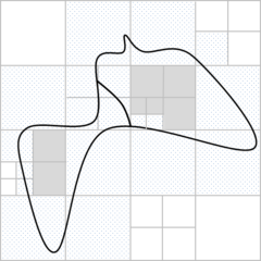
|
| Figure 17: 2D example where the three kinds of cells can be identified. The black curved line defines the contours of a domain formed by two surfaces (which are in contact), and the light gray lines represent the octree. Outer cells are the white ones, interface cells are marked with dots, and inner cells are colored in gray. |
In the frame of this work, the octree cells are classified in three categories:
- Interface cells. These are the cells colliding some input boundary entity. This means that some input boundary entity is inside them, or intersects them. Also the cells containing a forced node (Section 5.3.2) are considered as interface cells.
- Outer cells. These are the cells which are completely out of the domain to be meshed and they do not contain any forced node.
- Inner cells. These are the cells which are not interface or outer ones. These cells can be identified with some volume of the domain, as they are totally inside one volume.
Figure 17 shows a 2D example where the three kinds of cells can be identified.
3.3.2 Octree positions and nodes
As it is explained in Section 3.3.3, tetrahedral elements will be generated following a pattern from the octree. The nodes of these tetrahedra are called octree nodes and they are assigned to some predefined positions in space: the octree positions. Each cell has 27 octree positions corresponding to the vertices of the cell (8), the center of the cell (1), the center of its edges (12) and the center of its faces (6). A graphical view of the octree positions of a cell is shown in Figure 18.
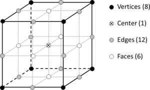
|
| Figure 18: Octree positions of an octree cell. The cell is represented by the black lines. |
It has to be noted that an octree position can be shared by more than one cell, as it can be seen in Figure 19.
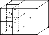
|
| Figure 19: Linear octree positions of a part of an octree. White dots are center of cells, and black dots correspond to vertices of cells. |
The linear positions of an octree cell are defined as the ones corresponding to the vertices and the center of the cell. The other positions are called quadratic positions. As an extension, the term of linear or quadratic octree node can be used to refer an octree node associated to a linear or quadratic cell position.
When referring to the whole octree, a linear position (or octree node) is the one which is linear in some cell. It has to be noted that an octree node can be linear regarding one cell, but quadratic from the point of view of another cell containing it. The linear octree positions of a part of an octree are shown in Figure 19 as an example.
It is important to note that not all the octree positions are forced to have an octree node associated, but all the octree nodes are linked to an octree position.
In Section 5.3.2 the concept of forced node is introduced. It basically corresponds to a node linked to an octree position, but occupying a different position in space.
3.3.3 Tetrahedra patterns
Parting from a given octree configuration, there are several possible tetrahedra patterns to be applied in order to split it. One important consideration is that the pattern chosen must fill the space with tetrahedra in a conformal way: it must not leave hanging nodes. A hanging node is a node lying on an element not being a vertex of it (it is on an edge or a face).
The option chosen in this work is based on the body centered cubic (BCC) lattice, which lead to a space-filling tetrahedra [45]. The use of BCC patterns linked to octree structures is quite natural considering the spacial distribution of the octree, and was proposed by [DBLP:conf/imr/Fuchs98,NME:NME616]. This option fills the space in a conformal way with a set of identical high quality tetrahedra: dihedral angles are or degrees, and edge lengths are 1 and times the cell size. This provides the tetrahedra with an edge ratio of (the ratio of the longest and shortest edges of the element).
A BCC lattice based pattern is local in the sense that each tetrahedra generated only depends on one cell and one of its neighbor. A pattern only depending on each cell (independent from the neighbor ones) would be more efficient for parallelization. However, this kind of patterns often provides with a lower quality tetrahedra (although their quality is acceptable) and a larger number of them [46].
The BCC lattice is defined in a regular grid (an octree with all its leaves equal-sided). As the octree used in the proposed method is not regular (it has leaf cells in different levels), other tetrahedra patterns must be defined.
To reach a tetrahedra mesh with no hanging nodes, all the linear octree nodes are used, and (in case they exist) the forced nodes linked to quadratic positions (forced nodes are defined in Section 5.3.2).
Basically, the tetrahedra pattern proposed focuses the tetrahedra generation cell by cell, and focusing on one cell, using its six faces independently. The only information required to generate the tetrahedra from a face of a cell is: the octree nodes of the face , the center octree node of the cell and the neighbor cell of from the face , denoted by .
As explained previously, the octree used is balanced (it accomplishes the constrained two to one condition). This ensures that the level of is one less, equal, or one more than the level of . These three configurations lead to the different tetrahedra patterns:
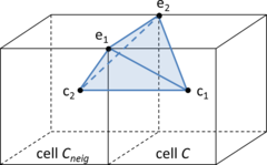
|
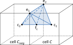
|
| (a) | (b) |
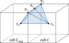
|
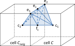
|
| (c) | (d) |
| Figure 20: Tetrahedra pattern in case where cell has the same level as . Tetrahedra generated from edge () of common face between and in different situations. (a) No quadratic octree nodes involved: one tetrahedron is generated (). (b) Octree node in the center of face : two tetrahedra are generated( and ). (c) Octree node in the center of edge : two tetrahedra are generated( and ). (d) Octree nodes in the center of face and edge : four tetrahedra are generated(, , and ). | |
- and have the same level (this means they have the same size). In this configuration the center node of is used to build the tetrahedra. Taking into account that the face (the face in contact between and ) has four sides (edges), from each edge from the face one, two or four tetrahedra are generated, depending on the possible presence of octree nodes in quadratic positions. The tetrahedra generated under each situation are shown in Figure 20.
The minimum dihedral angle of the tetrahedra generated in this configuration is degrees, and it occurs when some node in a quadratic position is used.
This case involves the creation of tetrahedra in two cells. Hence, only one of them should create them to avoid repetitions. The criteria used is that cell creates the tetrahedra only if it is lower than , otherwise the tetrahedra will be created by . Considering two leaves ( and ), is lower than if the coordinate of the center of is lower than the coordinate of the center of . If the coordinates are equal, the coordinate is checked, and if it is also equal, the coordinate is used to compare the cells. It has to be noted that, because of the characteristics of the octree structure, there cannot be two leaves with their centers in the same position.
- has one level more than (this means is bigger than ). In this configuration eight tetrahedra are created from the face . These tetrahedra are shown in Figure 21(a). It has to be considered that if is bigger than , the constrained two to one condition ensures that there will be four cells neighbors of in the other side of .
The minimum dihedral angle of the tetrahedra in this configuration is degrees.
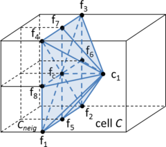
|
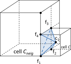
|
| (a) | (b) |
| Figure 21: Tetrahedra pattern in case where cell has different level than . (a) is bigger than : 8 tetrahedra are generated (, , , , , , and ). (b) is smaller than : two tetrahedra are generated( and ). | |
- has one level less than (this means is smaller than ). In this case two tetrahedra are created from the face , shown in Figure 21(b). Note that this configuration could build the two tetrahedra crossing the face by diagonals or . To ensure the final mesh to be conformal, the diagonal chosen is the one passing by the octree node which is the center of face in .
The minimum dihedral angle of the tetrahedra in this configuration is degrees.
It can be seen that the quality of the tetrahedra generated using these patterns depends on the configuration chosen, but it is always very good: the minimum dihedral angle of any tetrahedra coming from this predefined patterns is degrees.
The case where a cell has no neighbor by one of its faces occurs in the cells in contact with the boundaries of the octree root. This case is not considered because the building of the octree root (Section 5.2.3) ensures these kind of cells are totally out of the domain to be meshed, so they are not used to generate any tetrahedron.
3.4 Geometrical intersections
Geometrical intersections play a key role in the new meshing algorithm and affect several parts of it. This section focuses in defining how this intersections are considered. Their treatment has special interest when the input boundaries are non-watertight.
The intersection operation involved in the algorithm is typically the one between a segment and the surface entities defining the contours of a volume. This segment is understood as a portion of a straight line between two points. Depending on the part of the algorithm, it could be referred with different names such as edge (when talking about tetrahedra or triangle edges) or ray (when talking about ray casting operations). In this document some figures are based in 2D examples for clarity purposes. The equivalent intersection operation in these cases is between segment and line entities defining the input boundaries.
| ||||||||||||
| Figure 22: Types of intersections between a segment and a surface entity. Crosses are the intersection points. (a) No intersection. (b) type intersection. (c) type intersection. (d) type intersection. (e) and (f) type intersection; the red thick part of the segment is co-planar with the surface entity. |
Five situations are distinguished when evaluating the intersection between a segment and a surface entity (a graphical interpretation of these cases using simple examples is depicted in Figure 22):
- No intersection: the segment and the surface entity do not intersect (Figure 22(a)).
- Single intersection ( type): they intersect in one point within the surface entity (Figure 22(b)).
- Contour intersection ( type): they intersect in one point laying on the contours of the surface entity (Figure 22(c)).
- Tangent intersection ( type): they intersect in one point tangentially to the surface entity (Figure 22(d)) and the segment remains in the same side of the surface entity at both sides of the intersection point.
- Co-planar intersection ( type): the segment and some part of the surface entity are parallel and the distance between them is zero. This case can be split in two:
- Tangent ( type): before and after the intersection, the segment remains at the same side of the surface entity (Figure 22(e)).
- Intersected ( type): if the case is not accomplished (Figure 22(f)).
Analytically, the type of intersection has an infinite number of intersection points. As it will be seen in further sections, these intersection types only take relevance in the node coloring process (Section 4), that determines inside which volume a node is. For this reason the treatment of type intersections is detailed in Section 4.2.
Types , and have only one intersection point. However, as the contours of a volume may be formed by more than one surface entity, each intersection may involve a different number of intersection points (one for each intersected surface entity). This situation is illustrated in the 2D examples of Figure 23 (as a 2D example, line entities play the role of surface entities in 3D). In Figure 23(b) a intersection type has two intersection points (one for each intersected line entity), as well as in Figure 23(c) with the type intersection.
| ||||||
| Figure 23: Line entities enclosing surface intersected by a segment (bounded by two dots) presenting different intersection types. Intersected line entities are drawn in dotted line. (a) intersection type. (b) intersection type. (c) intersection type. |
These cases are characterized by the fact that all the involved intersection points are really close one from each other. Theoretically, all the intersection points should be in the exact same position, but because of the tolerances involved in the numerical computation of intersections this cannot be guaranteed. The tolerance is defined in order to determine if a collection of close intersection points corresponds to the same intersection: if all of them are within a distance lower than , they are collapsed into a multiple intersection point (MIP). The value of is a portion of the model bounding box size:
|
|
(3.1) |
being the length of the minimum side of the model bounding box, and a real value between zero and one. The value used in the present work for is detailed in Section 6.7.
The position of the MIP corresponding to a collection of intersection points is the mean position between all of them. In the present work, when evaluating the intersection point between a segment and the contours of a volume, in cases where there are intersection points close enough, their MIP is considered instead of them. This matches with the theoretical number of intersection points corresponding to each intersection type: and intersection types have only one intersection point (a MIP).
3.4.1 Non-watertight geometries
For non-watertight geometries, special cases may be treated when evaluating the intersection between a segment and the contours of a volume. There are basically two specific intersection types (a 2D example of this cases is depicted in Figure 24):
- Overlap intersection (W type). This situation happens when the part of the boundaries of the domain where the segment intersects is defined by more than one overlapped surface entity (Figure 24(a)).
- Gap intersection (G type). This situation happens when the part of the boundaries of the domain where the segment intersects has a gap (Figure 24(b)).
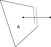
|
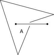
|
| (a) | (b) |
| Figure 24: Intersection between a segment and the line entities enclosing surface A in non-watertight situations: (a) overlap (W intersection type) and (b) gap (G intersection type). | |
For the W intersections type, the corresponding MIP of the intersection points involved is considered. For this purpose, in cases where non-watertight geometries define the domain, takes the value of . This parameter must be provided in the input data and is a characteristic length of the gaps and the overlappings of the model. must be an upper limit of the distance between overlapping entities. The MIP corresponding to the 2D example of Figure 24(a) is shown in Figure 25(a).
G intersections do not provide with any intersection point. However, as it will be seen in further sections, there are cases where the extremes of a segment are known to be inside different volumes. Situations where both extremes belong to different volumes indicate that there should be an intersection point although it is not detected. In this cases the gap intersection point (GIP) is created. Considering the surface entities surrounding the segment, the closest point from each surface entity to the segment can be computed. The GIP takes the position of the closest one. The GIP corresponding to the 2D example of Figure 24(b) is shown in Figure 25(b).

|
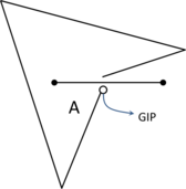
|
| (a) | (b) |
| Figure 25: Treatment of intersections of non-watertight geometries depicted in Figure 24. (a) MIP corresponding to the W intersection depicted in Figure 24(a). (b) GIP corresponding to the G intersection shown in Figure 24(b). | |
In the present work, the intersection point between a segment and the contours of a volume could be a single intersection point, a MIP or a GIP.
4 Coloring algorithm
As explained in Section 2.5, space decomposition meshing methods use a regular grid (in our case, an octree) over the domain to be meshed. The regular grid is larger than the domain, so at some point of the algorithm, this family of methods are forced to use a strategy to know if a given position of the grid is inside or outside the domain.
The coloring operation consists in determining where the entities are in the topological sense. This is, to determine whether each entity is inside a volume, out of the domain or laying on an interface entity between volumes. Applied to points, this operation is known in the literature as the point-in-polygon (PIP) problem [47,48,49].
In the presented meshing method, the coloring operation is applied to nodes (the case explained in this section) and to tetrahedra (as explained in Section 5.3.7).
This is one of the key points of the meshing algorithm, as it is not obvious to determine if a point in the space is inside a volume or not when the contours of the volume are non-watertight. Actually, if the contour of the volume has gaps, the concept of interior or exterior of the volume is not even defined from the topological point of view.
It has to be noted that several existing octree-based methods are focus on meshing a domain formed by a single volume. In this work arbitrary domains with several volumes are meshed at once, so coloring a node is not reduced to identify if it is inside or outside the domain: it has to be determined inside which volume (or interface entity) is.
4.1 Coloring strategies
There are several ways of coloring points considering a watertight definition of the volumes. These cases have some clear advantages as the contours of each volume can be oriented coherently (towards the interior or the exterior of the volume). This orientation provides with valuable information at the time of determining if a point near the contour entity is inside or outside the volume.
However, this work is focused on non-watertight geometries. This implies that a coherent orientation of the contours of a volume cannot be guaranteed. To deal with such geometries it is common to work with a voxelization of the model [50,51,52]. These strategies aim to converting the non-watertight geometries into water-tight ones in order to be able to apply the coloring strategies of points. A voxel representation of a model is a regular grid (typically axis aligned and isotropic) where each voxel contains a topological information. In the case of study, it contains the color of the voxel. If a voxel is intersected by a surface entity it has the color of that surface (lets call it a contour voxel), otherwise it has the color of the volume it is into (inner voxel), or the color of the outer part of the domain if it is not inside any volume (outer voxel). All the points inside an inner voxel can be considered as interior to the corresponding volume. An example of voxelized 2D model is shown in Figure 26.
| ||||||
| Figure 26: Example of three voxelizations of a 2D model. The model has a gap in its contour and it is represented by the black curved line. Contour voxels are drawn in red. (a) The size of the voxels is large enough to close the gap of the domain: the topology of the voxelized model is watertight. (b) The size of the voxels is too small, so the gap of the domain is not closed. (c) The size of the voxels is too large: the gap is closed, but the final topology does not represent correctly the domain. |
The advantage of working with voxelized models is that, depending on the size of the voxel, the topology of non-watertight geometries can be improved. If the gaps of the input boundary or the distance between overlapped contour entities is lower than the voxel size, the voxeled model may close the gaps or join the overlapped entities. This situation is shown in Figure 26(a), where the voxelized model presents a closed set of inner voxels (with no gap in its contour). As a drawback, the voxelized model can neglect some important topological information of the domain: the topology of the voxelized model shown in Figure 26(b) represents exactly the topology of the model (with its gap). Despite the size of voxels used in Figure 26(c) is large enough to close the gap (which is desirable), it represents an undesired topology, as it includes different sets of unconnected inner voxels.
The problem is that the voxel size needed to represent correctly the topology of the model cannot be estimated a priori and it may not be valid for the whole domain. Figure 26 shows that three different voxel sizes lead to three different topologies of the same domain.
If the voxelized model is watertight, one strategy for the coloring of the voxels is by propagation [50]. This strategy consists in the following steps:
- Determine all the contour voxels (the ones colliding a contour entity).
- Determine one (and only one) voxel interior to each volume solving the corresponding PIP problem.
- From a known inner voxel, assign its color to its neighbour voxels if they are not contour ones.
- Repeat the last step until all the voxels have color.
This propagation method is totally robust in watertight representations and has the advantage of solving very few times (one for each volume) the PIP problem, which can be computationally expensive. However, it has the drawback that is not naturally parallelizable. Only the voxels which are neighbour of a determined voxel (a voxel with a known color) can be colored at a time.
Voxelizing the model can help the coloring strategy as it can make the model watertight, enabling the use of the propagation method (which requires the solving of PIP problem only in a few points). However, it has been seen that even the voxelized model may be non-watertight. In this case the color propagation cannot be done, so the PIP problem has to be solved for each one of the points to be colored (in our case, the octree nodes).
4.1.1 Ray casting
The solution chosen in this work for coloring the octree nodes is based on the ray casting technique. The ray casting algorithm was first developed by Arthur Appel for rendering purposes in 1968 [53]. It proposes a solution for determining the visibility of a 3D object from a given point of view, and uses this information to paint a representation of the 3D object in a 2D image (made of pixels). The idea behind ray casting is to shoot rays (straight lines) from the point of view (one per pixel) and find the closest part of the object intersecting the ray. The algorithm needs to compute first all the intersections between a ray and the contours of the object (surface entities), and then get the closest to the point of view.
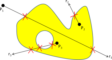
|
| Figure 27: 2D example of the ray casting technique to solve the PIP problem. Point is considered outside of the polygon because ray has an even number of intersection points (2). Points and are considered inside of the polygon because rays and have an odd number of intersection points (1 and 3 respectively). |
Despite the first applications of ray casting were focused on rendering of 3D objects, its use has been generalized for several purposes following the philosophy of analyzing the intersection points between the ray and given 3D objects.
A common use of the technique is to solve the PIP problem. Among the several existing methods to solve this problem [47,48,49], a classical approach is the ray intersection method [47]. It consists in tracing a random ray from the point of analysis and compute the number of intersections between it and the contours surface entities. If the number is even, the point is outside the domain, and if it is odd, it is inside.
A 2D example illustrating the application of ray casting technique to solve the PIP problem is depicted in Figure 27. In this example, is considered outside of the polygon because the ray has two intersection points (an even number). Points and are considered inside of the polygon because their rays ( and ) have an odd number of intersection points (1 and 3 respectively).
4.2 Ray casting-based proposed technique
As pointed out previously, in the present work the coloring process of a node must identify not only if it is inside or outside the domain, but also the specific volume of the domain it is into. To fit this requirement, the ray casting method in this work focuses more on the topological information of each intersection rather than in the number of them. Following this philosophy, the proposed method consists in tracing rays in space and take care about the intersection of these rays with the contours of the volumes: if a ray intersects the interface between volumes A and B, it can be ensured that, near the intersection point, at one side of the intersection point the ray will be inside A, whereas at the other side it will be inside B. Following this principle, if we move along a ray from a point which color is known, we can color all the points of the ray just looking at the intersections of it with the contours of the volumes. Figure 28 shows a 2D example where a ray beginning in the outer part of the domain is colored in different parts corresponding to the contours it is intersecting.
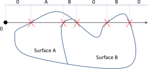
|
| Figure 28: A 2D example of coloring parts of a ray (represented by the black arrow). The black dot is the beginning of the ray which color is known: . The crosses are the intersection points between the ray and the contours of the surfaces A and B (which are the ones forming the domain). In the upper line the color of the different parts of the ray is shown. |
It is important to note that the presented technique only need the topological information of the surface entities: which volumes they are intersecting. Other techniques require the use of normal vectors in some points, or a given connectivity among the surface entities defining the contours of the domain. This is crucial considering the proposed algorithm must work with non-watertight definitions of the volumes. In these cases it is not obvious to define the oriented normal of a surface entity pointing towards the inner or the outer part of a volume.
4.2.1 Pathological configurations
The ray casting technique presents some pathological configurations [49] for the PIP problem. One of these is the case when the intersection between the ray and the volume boundaries is done tangentially (T type intersection defined in Section 3.4). In this situation the ray intersects the boundaries of the geometry, but both sides of the intersection are in the same volume. To solve this problem, this kind of intersections (tangentially to the boundaries of the volumes) are not taken into account for coloring the regions of the ray. Figure 29(a) shows an example of this pathological case: both sides of the ray from the dark intersection point are inside surface B, although there is an intersection point.
Another pathological configuration occurs when the intersection point is a point of the boundary interfacing more than two volumes (in 2D case, more than two surfaces). This is the case shown in Figure 29(b). For notation purposes, this kind of intersections are referred as a M intersection type.
If a intersection is detected in a ray, a color has to be chosen for the following part of the ray (from the intersection point on). The strategy followed to decide this color is explained in the Implementation chapter (Section 4.3.1). It is based on a try and error approach considering all the possible colors.
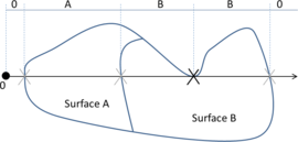
|
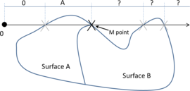
|
| (a) | (b) |
| Figure 29: 2D examples of pathological configurations for the ray casting technique. (a) Both sides of the ray from the dark cross intersection are colored equally (surface B) although there is an intersection point because the ray is tangent to the contours in it. (b) M point is interface between surface A, B and (outer part of the domain), so the color of the right part of the ray cannot be set. | |
The case of co-planar intersections ( and intersection types defined in Section 3.4) presents also a pathological configuration for the ray casting technique. In these cases, the part of the ray co-planar with the boundaries must be colored with the color of the interface itself. In this case, the color does not correspond to a volume, but to an interface between volumes. 2D examples for and intersection types between the ray and the boundaries of a model is depicted in Figure 30. The end point of the co-planar part of the ray is considered as an point from the coloring point of view.
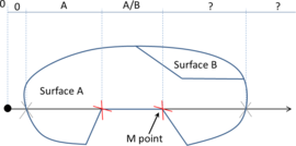
|
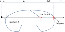
|
| (a) | (b) |
| Figure 30: 2D examples of co-planar intersections of the ray. (a) intersection type. The color at the right part of the point could be or zero. (b) intersection type. The color at the right part of the point could be , or zero. | |
For non-watertight contours of the domain volumes, two more pathological configurations affect the ray casting technique. They are related to the possible gaps and overlapping entities in the contours (G and W intersection types defined in Section 3.4):
- If a ray passes through a gap of the contours of a volume (G type intersection), it does not detect that is entering into the volume, so it would assign the following regions an invalid color. This is the case shown in Figure 31(a), where the ray casting technique only identifies two zones in the ray separated by the intersection point: the left region as outer, and the right one as inside surface A.
- When a part of the contour of a volume is overlapped (W type intersection), if a ray intersects the contour by that region, it intersects more than one time the contour. The case where the distance between the overlapping entities is smaller than presents no problem, as only one intersection point is considered: the MIP. This can be understood as a local voxelization of the model, as the topological information of different entities is collapsed into one data (voxel). The case where is greater than disturbs the coloring operation as the color of the ray changes two times instead of one. This is the case shown in Figure 31(b), where the part of the ray inner to surface A is colored as outer because of the two close intersections highlighted in the figure.
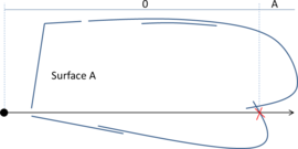
|
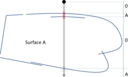
|
| (a) | (b) |
| Figure 31: 2D examples of pathological configurations for the ray casting technique with non-watertight domains. (a) G type intersection of the ray. The part of the ray inside the surface A is not colored as A because the ray has not intersected its boundary entities. (b) W type intersection of the ray. The part of the ray inside surface A is colored as zero because the ray intersects two times the boundary in the same region (crosses). | |
Both pathological cases (gaps and overlappings greater than ) can lead to set the ray as invalid. An invalid ray is a ray with some coloring contradictions. There are two kinds of contradictions, depicted in Figure 32(a) and (b):
- The last part of the ray (from the last intersection point to the outer part of the bounding box of the model) has a color different than zero (see Figure 32(a)). Considering the principle that the parts of the ray outside the bounding box of the domain must be outer, the beginning and end of the ray must be outer (color zero).
- A part of the ray colored as ends in an intersection point with a surface entity not interfacing the ith volume (Figure 32(b)).
| ||||||
| Figure 32: Types of invalid rays (crosses are intersection points). (a) The last part of the ray is colored as , but it should be zero.(b) At the dark cross intersection point the ray should arrive with color or , as these are its interfacing surfaces, but its color is zero. (c) Rays to be canceled because they provide with different colors to a given position. |
Situations of invalid rays can also happen even if the contours of the domain are watertight, taking into account that the intersection operations in 3D are done numerically, so they depend on tolerances. Some specific configurations of the ray and the contours may lead to an invalid ray.
4.2.2 Adaptations of the method
A special kind of rays are the Cartesian rays, which are straight and parallel to the , and directions. The ray casting technique can be applied to any kind of ray, but in the proposed algorithm Cartesian rays are used because they simplify the intersection operations, and they take profit on the spacial distribution of the nodes provided by the octree structure (this aspect will be seen in more detail in Section 4.3).
Taking into account that the domain to be meshed is totally inside its bounding box, the octree nodes which are outside it can be directly colored as zero (they are out of the domain) without the need of any coloring process. All the other octree nodes are colored using rays which begin out of the model bounding box, so as the color of the initial point of the ray is known: zero. The color of a node is directly the color of the part of the ray the node is into.
As there are situations in which a ray is considered as invalid to color a point because of a pathological configuration, the following strategy is applied in order to color all the octree nodes:
- For each octree node, three Cartesian rays (one for each direction , and , from the lower to the higher coordinate) passing by the position of the node are shooted from the outer part of the bounding box of the domain.
- Each one of these three rays can be invalid or valid. If it is valid it provides with a candidate color for the octree node. This opens the following cases:
- There is only one valid ray. The node is colored with the color given by the ray.
- There is more than one valid ray and they give the same color. The node is colored with that color.
- There is more than one valid ray and they give different colors. A 2D example of this case is depicted in Figure 32(c). In this case the three rays are canceled. To cancel a ray means not to use its color information. It has to be taken into account that a ray can be used to color more than one node, as some nodes may be aligned with the Cartesian directions. In this case, canceling a ray also affects the other nodes it passes throw.
- The three rays are invalid. In this case the node is not colored.
- At this point of the process there may be nodes with no color. These ones are colored using a local ray casting. This operation consists in launch a ray (not a Cartesian one) from a neighbor node with a known color to the node itself. The color is set evaluating the intersections of this local ray with the input boundaries. A 2D example of this local ray casting operation is shown in Figure 33. It has to be noted that the situation where the node cannot be colored with the Cartesian rays is rather improbable, as it should imply the coincidence of pathological situations in the three directions of the space aligned with the node.
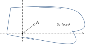
|
| Figure 33: A 2D example of local ray casting. A non watertight representation of surface A is shown. The two Cartesian rays passing by the black dot (drawn with dotted arrows) are not valid. The color of the white dot is known (inside surface A). As the ray from the white dot to the black one has no intersection with the boundaries of the domain, the color of the black dot is also set to A. |
This strategy have been proved in several examples, and it solves successfully the coloring process for the octree nodes with pathological configurations for the ray casting technique. The use of three rays for each node provides with a redundancy minimizing the possible effect of an invalid undetected ray.
4.3 Implementation of nodes coloring algorithm
This section is focused in the implementation of the algorithm explained in Section 4.2.2 for nodes coloring. It requires three Cartesian rays for each one of the nodes in order to color them (determine where they are topologically). Applying this algorithm to a general cloud of nodes would imply to compute the intersections of rays. However, as the nodes of the tetrahedra mesh treated in this work are octree nodes, most of them are placed on regular positions in space, aligned with the Cartesian directions. To take advantage on this configuration, one ray can be used in the coloring of several nodes: all the ones aligned with a Cartesian direction. Following this strategy an important time saving is achieved in the nodes coloring operation.
It is important to note that only the nodes with unknown color must be colored following the presented algorithm. The octree nodes with known color before the coloring operation are:
- The forced nodes (section 5.3.2); as they are linked to an entity coming from the input data, they directly have the color of the corresponding input geometrical entity.
- The octree nodes outside the bounding box of the domain. These ones are outer nodes, so their color is zero.
A 2D example of the rays used to color the nodes of a given configuration of a quadtree is shown in Figure 34. In the example, there are nodes to be colored and rays are used ( for direction and for direction).
| ||||||
| Figure 34: Rays used to color the quadtree nodes of a 2D example. The contour of the domain is the solid black line and the dotted line represents its bounding box. Rays are represented with red arrows. (a) Quadtree configuration with all the octree nodes represented. The black nodes are forced nodes. (b) The rays used in direction to color the nodes. Only the nodes to be colored are plotted in order to clarify the figure. (c) The rays used in direction. |
The implementation of the coloring operation is based in the following steps:
- Creation of all the rays. For each one of the three directions of the space (, and ), the coordinate of each one of the nodes to be colored is considered. Then, one ray is created for each one of the coordinates. This process generates a collection of rays. Each one of the rays has the following information:
- The alignment direction.
- The two coordinates corresponding to the plane perpendicular to its direction.
- The nodes it passes through, sorted from lower to upper coordinate in the direction of the ray.
- Color the rays and set the contribution to each node. In this step each one of the rays is colored. It has to be noted that this process is fully parallel, as each ray is totally independent from the others. In this process all the intersections between the ray and the input boundaries are computed. They are sorted from lower to upper coordinate, dividing the ray in different parts corresponding to the regions between intersection points. Looking at the interfaces intersecting at each intersection point the color of the parts of the ray can be set. Pathological situations in the intersection operations are detailed in Section 4.3.1. As explained in Section 4.2.2, each node has three possible colors, corresponding to the three Cartesian rays passing through it. At this point, the color contribution of the ray is set to all the nodes it passes through.
- Determine the invalid rays. As explained in Section 4.3.1, the invalid rays are identified. Then, the rays with contradictions in one node are canceled.
- Set the color of the nodes. The process described in Section 4.2.2 is used to determine the color of the node considering its three color contributions: if there is some valid ray the color is set automatically, otherwise, the local ray casting is performed. In case the local ray casting provides with different candidate colors (from the local rays from different neighbors), a voting process is performed: the color set is the one given by more neighbors.
4.3.1 Pathological situations
In this section the strategy followed to solve the pathological situations for the ray casting technique defined in Section 4.2 is detailed. These situations are related with the , , , and intersection types and the intersection points.
In all these situations the intersection point is a (Section 3.4). Actually, the intersection type (situation where the ray passes through a gap in the boundaries) involves a , but this kind of intersections is not solved in the present approach because trying to find the corresponding to all the parts of the ray not intersecting the input boundaries would be too computationally expensive. Leaving this situation as unsolved could lead to rays declared as valid, but giving wrong information in terms of coloring. It has to be noted that if this situation occurs, it does not mean necessary that an invalid color will be assigned to the nodes. As the three Cartesian rays passing by a node contribute to the decision of its color, only in cases where the three rays are considered valid, provides with wrong information and this information is compatible (within the three rays), the color of the node would be wrong. This is a rather improbable situation, which have never happened in the examples run in this work.
A MIP in a ray indicates the presence of a pathological configuration. Each intersection point has the information of the two volumes interfaced by the surface entity where it is (the interfacing volumes of the intersection point). The interfacing volumes of a MIP are the union of the interfacing volumes of each intersection point involved, so a MIP can have two or more interfacing volumes.
In Section 4.2 the situation of intersection types (co-planar ones) is explained. They correspond to a intersection point at the end part of the co-planar part of the ray. Considering that the presented algorithm uses linear triangle elements as surface entities for defining the boundaries of the domain, the situation where the ray is co-planar can be detected easily. If geometrical surface representations (line NURBS) are used for defining the contours of the volumes, solve this situations becomes much more difficult. For coloring purposes, the co-planar part of the ray takes no relevance, as it is ensured there will be no node to be colored there. If a node is so close to a surface entity it is a forced node in interface (Section 5.3.2), so its color is already set without the need of ray casting technique. The problematic situation comes at the time to color the following part of the ray (next to the co-planar one), where a color have to be assigned among the corresponding interfacing volumes.
When a MIP (a pathological configuration) is detected, its type has to be determined (, , or ) in order to apply the right strategy to color the following parts of the ray from that point on. For this purpose, a sort of auxiliary local rays are built: the surrounding segments. These are segments parallel to the ray at a distance of it. In the present implementation, a number of surrounding segments has been chosen following the Cartesian directions. Longitudinally, the surrounding segments are centered in the MIP position and have a length of , being the distance to the closest intersection point of MIP (in the ray). An example of the surrounding segments of a ray is shown in Figure 35. In this example the ray intersects two triangles by its contour edge, so it is a intersection type.
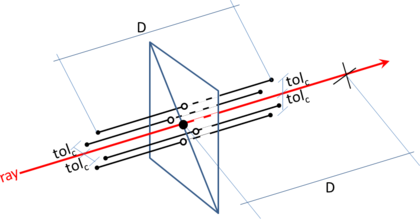
|
| Figure 35: Surrounding segments of a ray around a MIP. The two triangles represent a part of the input boundaries. The black dot is the MIP and the white ones are the intersection points between the surrounding segments and the input boundaries. The black cross is the nearest intersection point of the ray to the MIP. |
Then, the intersection points between the surrounding segments and the input boundaries are computed. Considering them and the MIP interfacing volumes, the following cases should be accounted for distinguishing the type of pathological configuration:
- Case I: there are more than two interfacing volumes among the ones of the MIP and the ones of the intersection points of the surrounding segments. This case corresponds to the intersection type.
- Case II: case is not accomplished (so only two interfacing volumes are involved) and some surrounding segment has no intersection point. This case corresponds to the intersection type.
- Case III: when cases and are not accomplished. This means that all the surrounding segments have intersection points, and there are only two interfacing volumes involved. The following sub-cases are considered:
- Case IIIa: each one of the surrounding segments have only one intersection point (MIP or single one). This case corresponds to the intersection type.
- Case IIIb: all the surrounding segments have only one intersection point and some of them is a MIP (this means all the intersection points of the surrounding segment are enclosed in a distance ). This case corresponds to the intersection type.
- Case IIIc: there are surrounding segments with more than one intersection point. This case corresponds to the intersection type.
Actually, cases IIIa and IIIb could be merged, as case IIIb is included in IIIa. The differentiation has been made only to highlight that a intersection type always implies a MIP, and the one can present a MIP or not in the surrounding segments. This is not relevant because the treatment of and intersection types is analogous for coloring purposes.
A graphical interpretation of these cases in a 2D example is illustrated in Table 4.3.1. As a 2D cases, only two surrounding segments take sense for a MIP.
| Case I: there are three interfacing surfaces (, and zero) involved in the intersection points of the surrounding segments. intersection type. | 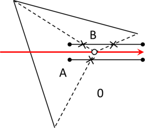
|
| Case II: all the intersected entities have the same interfacing surfaces ( and zero), and there is one surrounding segment with no intersection. intersection type. | 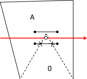
|
| Case IIIa: each of the surrounding segments intersects the boundaries in one point and all the interfacing surfaces are the same ( and zero). intersection type. | 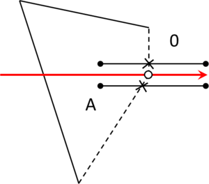
|
| Case IIIb: all the surrounding segments can create a MIP (its intersection points are closer than ) and all the interfacing surfaces are the same ( and zero). intersection type. | 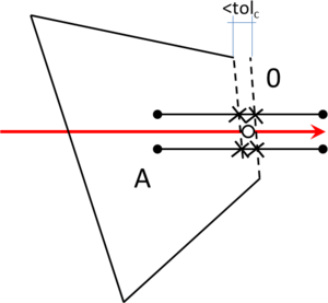
|
| Case IIIc: Some surrounding segment has more than one intersection point. intersection type. | 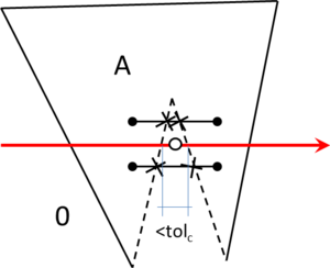
|
Different cases for surrounding segments for identification of intersection types corresponding to a MIP (white dot) in a 2D example.
Once the type of pathological intersection has been determined, the following strategy is carried out to color the following part of the ray (the one next to the MIP):
- type intersection. In this case the color of the ray is not changed in the following ray part.
- and type intersections. In this case the color of the ray is changed accordingly with the interfacing volumes: as there are two interfacing volumes ( and ), if the previous part of the ray was colored as , the next one is and viceversa.
- type intersection. This case is the more complicated one. Considering the interfacing volumes of the corresponding MIP and the color of the previous part of the ray, the following part of it can have any color among the rest colors. The strategy chosen is based on a try and error approach: rays are shooted from the MIP, one for each possible color, and if one of them is valid, it is taken as the good one. If no one of them is considered valid, then the whole ray is set as invalid.
There is one situation not solved by the presented strategy. It is a mix between the and the intersection types. It occurs when the ray passes tangentially to two parts of the boundaries of a volume at the same point. A 2D example of this situation is shown in Figure 36. If the corresponding surrounding segments have one MIP each one, it corresponds to the case IIIb, so the intersection would be considered as and the color of the ray would change when it should remain with the same color (as if it was a intersection).
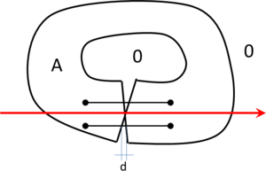
|
| Figure 36: Pathological situation where the analysis of the surrounding segments can lead to erroneous classification of intersection type if . |
4.3.2 Computation of distances
As explained in previous sections, this work proposes a meshing algorithm for body fitted meshes and for embedded ones. The later ones are used in embedded and immersed methods, and require for the nodes of the mesh their distance to the input boundaries in addition to their color (Section 5.2). This section focuses in the computation of these distances for the embedded meshing algorithm.
As explained in Section 5.2.1, the computation of distances from the nodes of the tetrahedra mesh to the input boundaries for embedded methods takes advantage on the ray casting technique used in the coloring algorithm. This is mainly because the Manhattan distance [54] has been chosen for approximating the distance for far nodes (nodes further than a given distance of the boundaries of the domain). The Manhattan distance between two points is the sum of the distances of the three Cartesian components of the vector defined by the points. As the rays used in the coloring algorithm are Cartesian, its use fits perfectly for this purpose.
To improve the efficiency in a parallel implementation of the method, each ray contributes with a distance to the nodes it passes through. This implies each node has three contributions of distances, as each node has three rays passing trough it (one for each direction: , and ).
The process of computing the distances from the nodes of the tetrahedra mesh to the input boundaries follows the steps detailed hereafter:
- Compute the exact distance to the input boundaries of the octree nodes belonging to an interface leaf of the octree. The exact distance is the one from the octree node to its closest coordinate onto the input boundaries. The strategy chosen to compute this distance profits from the octree itself. The surface entity from the input boundaries the closest coordinate is onto must collide an octree leaf containing the octree node. So only the surface entities colliding these octree leaves are considered at the time of finding the closest coordinate to a node.
- Set to the maximum possible distance the three distance contributions of the rest of octree nodes.
- Proceed with the ray casting technique corresponding to the coloring process. Apart from the color assignment to the nodes, an extra operation is performed in order to set the distances. Each ray launched in the coloring process has the information of its intersection points with the input boundaries, and the octree nodes it passes through (the ray nodes). Being the existing distance contribution of a ray node and the distance from the node to its closest intersection point in the ray, is equalized to if .
- Propagate the distance of each node within each ray. This step only affects the rays with more than one node. Let us consider the nodes of a ray sorted out by the coordinate corresponding to the direction of the ray. Being one of the nodes and and its previous and next nodes, , and are defined as their corresponding distance contributions of the ray. (For the first node only the is considered, and for the last one only the ). Two propagated distances are defined for each node:
- Update the distance contributions of each node. This operation consists in equalizing the three distance contributions of each node to the minimum one of them.
- Repeat Steps 4 and 5 (propagate and update) two more times. This two steps must be done a number of times equal to the dimension of the problem (in our case, three times). This is to allow a complete propagation of the distances from the nodes. As this propagation is done using Cartesian rays, the information provided by one direction is not passed to the other ones until the distance contributions are updated. A 2D example is depicted in Figure 37 where the iso-lines for distance are plot before and after the second propagate and update operation (as a 2D case, propagate and update operation must be done only two times). It can be seen (in Figure 37(b)), that the distances in the lower left and right part of the surface are not well computed. As the hole of the surface is not aligned with them, the second propagation and update operation is needed to compute correctly the distances to the boundaries of all the nodes (Figure 37(c)).
|
|
(4.1) |
|
|
(4.2) |
where is the distance between nodes and . Note that, as the nodes are aligned in the ray, the distance between them is directly the difference between their coordinates corresponding to the ray direction.
Considering each node of the ray, its distance contribution is set to the minimum between , and .
| ||||||
| Figure 37: 2D example for computation of distances to the boundaries. (a) Surface representing the domain. The surface is a square with a squared hole inside. (b) Iso-lines of distance to the boundaries of the surface when only one propagation and update operation have been done. (c) Iso-lines of distance performing the propagation and update operation two times. |
5 Octree based mesher
5.1 Introduction
This chapter present the octree-based mesher developed in this monography.
One of the requirements defined in Section 1.2.3 refers to the immersed [6] and embedded [7] methods. This family of methods uses the so called embedded meshes. An embedded mesh is a mesh of a part of the 3D space containing in its interior the domain to be simulated, but the mesh is not limited to the inner part of the domain and, furthermore, does not fit the contours of it. The effect of the contours of the domain in the results of the numerical simulation to be run is captured by the assignment of special boundary conditions in the mesh elements and nodes. Because of its nature, it takes no sense to talk about preserving features or topology preservation for embedded mesh generation.
On the other hand, there are the body-fitted meshes, which must capture precisely all the contours of the domain. They need a faithful representation of the boundaries preserving the geometrical features, the topology of the volumes of the domain, and forcing the nodes and elements to follow the shape of their contours.
The algorithm proposed in this monography considers the embedded meshing as a particular case of mesh generation where there is no need to apply any strategy for preserving geometrical features or volume topology. In this sense, the generation of embedded meshes will be easier than the generation of body-fitted ones.
The detailed explanation of the meshing algorithm requires the definitions of specific concepts and auxiliary algorithms explained in Chapter 3. In Sections 5.2 and 5.3 the meshing algorithm itself is presented for embedded and body-fitted meshes.
As a general view, the main steps of the mesher are pointed out hereafter. Let us consider that the input data for the mesher is the definition of the contours of the volumes of the domain to be meshed (from now on, input boundaries) and a given list of parameters (detailed in Section 3.1). The new embedded meshing algorithm can be summarized in five steps:
- Create an octree enclosing the domain.
- Refine the octree following some given criteria.
- Generate a tetrahedra mesh from predefined patterns from the octree.
- Find the volume containing each node of the mesh.
- Compute the distance of the nodes of the resulting mesh to the input boundaries.
The first three steps are directly related to the octree structure. The two other ones involve mesh operations that can be applied to any unstructured tetrahedra mesh independently on its generation method, although the octree structure can be used as an auxiliary tool in order to improve the efficiency of the algorithms. They are detailed in Chapter 4 and Section 5.2.1.
Concerning the body-fitted mesher, the four first steps are the same ones as for the embedded mesher (adding some extra refinement criteria to refine the octree in the second step), and the fifth step is replaced by the following three ones:
- Apply given mesh edition operations to fit into the tetrahedra mesh the sharp edges and corners to be preserved and the surface entities of the domain. These mesh edition operations are detailed in Sections 5.3.5 and 5.3.6, and they basically involve nodes movement and element splitting.
- Identify the volume each tetrahedra of the mesh is into. This part of the algorithm is detailed in Section 5.3.7.
- Improve the mesh quality if needed using make-up and smoothing operations. This step is optional, as it is only needed if the mesh quality is poor. It is detailed in Section 5.3.8.
All these specific steps related to the body-fitted mesher are also applicable to any unstructured mesh, independently on the generation method chosen.
An important aspect of the new mesher is that it generates the mesh of the whole domain at once, including all the volumes which are part of it. Other existing meshers are designed to generate the mesh of just one volume, so they generate the mesh of the whole domain on a volume by volume manner.
5.2 Embedded mesher
One of the objectives of the presented meshing algorithm is to generate meshes for embedded methods. This section is focused in the specific aspects of the algorithm for this kind of methods.
The main characteristic of embedded methods is that the mesh used is not body-fitted, and its nodes have the information of:
- where they are topologically (inside which volume or onto which interface between volumes);
- the distance they have to the contours of the domain.
Knowing if a node is inside or outside a volume is solved by the proposed coloring algorithm (Chapter 4), and the computation of distances also takes profit of that algorithm, as explained in the following section. Furthermore, it is common to apply these methods to domains where only one volume is involved, so only two colors take part: inside and outside.
Embedded meshes are mainly used in Computational Fluid Dynamics (CFD) simulations, where the behaviour of a fluid around solid bodies is studied. If the solid bodies are in movement, rather than remeshing the whole domain at each time step, this family of methods maintains the volume mesh static and updates the nodes information (color and distance).
5.2.1 Computation of distances
The distance function plays a key role in embedded methodology in order to apply the boundary conditions. It is common to combine the coloring and distance function into one signed distance function where negative distance indicates inside and positive distance indicates outside nodes. A direct result of this definition is the fact that the iso-surface representing the zero distance defines the approximated embedded boundary condition, as shown in Figure 38.
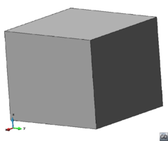
|
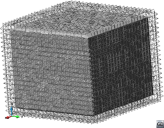
|
| (a) | (b) |
| Figure 38: (a) Surface entities defining a cube. (b) The cube representation via a zero iso-surface of the distance function in the tetrahedral embedded mesh generated. | |
To ensure the accuracy of the method the distance near the boundary and especially in cut elements must be calculated exactly. For the nodes far from the boundary the exactness of the distance becomes less important so, in order to reduce the computational cost, it is convenient to calculate the exact distance only for the points inside a given distance range from the boundary, and leave the rest with a maximum value (an upper distance limit). However, in cases with moving boundaries one may convect the distance function given the interface motion. In this procedure, having sharp gradients in distance functions can lead to numerical error and having a constant maximum distance near the boundary may affect the convergence and results. In order to deal with this problem an approximation of the distance function from a given distance of the boundary would be interesting.
In this work the exact Euclidean distance is calculated for the octree nodes belonging to the interface leaves. For the rest of them the Manhattan distance [54] is computed. It is an estimation of the exact distance given by Equation 5.1:
|
|
(5.1) |
where is the Manhattan distance between positions and , and represents the -coordinate of the vector. is the dimension of the space considered, in this case: three.
The Manhattan distance provides with the desired continuity and smoothness of the distance function in order to deal with moving objects with minimum distance calculation overhead. The reason to use this distance measure is to take profit on the coloring algorithm, as explained in Section 4.3. Cartesian rays are used for the coloring of the nodes, so using the distances onto the rays provides directly with the Manhattan distance.
5.2.2 Octree refinement criteria for embedded meshes
As explained in Section 5.1, one of the main steps of the meshing process is refine the octree following given criteria. The basic idea is that the octree must be refined in such a way that the application of the further steps of the meshing process ensures the accomplishment of the requirements to be covered.
In this section all the refinement criteria (RC) needed for embedded meshes are defined. It is important to highlight that all the octree refinement criteria defined in this section (the ones needed for embedded meshes) only depend on the desired mesh sizes and the topology of the octree itself (the balance criterion). This implies that the application of these refinement criteria does not need to consider the input boundaries. For notation purposes, the collection of all the refinement criteria defined in this section is called size refinement criteria.
5.2.2.1 Uniform size refinement criterion
Let us consider the bounding box of the model (). It is a parallelepiped with its faces parallel to the Cartesian axes (note that is not needed to be coincident with the octree root). is defined as the length of the smaller side of .
For given desired mesh sizes (via mesh size points or general mesh size parameter), lets define as the maximum of the desired mesh sizes entered in the input data. Then, is defined by Equation 5.2:
|
|
(5.2) |
If no size has been introduced in the input data, then is directly .
It has to be noted that because of the tetrahedra pattern definition (Section 3.3.3), tetrahedra sizes are directly related to the octree cells sizes. Actually, the size of the edges of the tetrahedra generated from a cell is always equal or smaller than the cell size. Refining the octree implies dividing by two some of the cells, reducing accordingly the corresponding tetrahedra size. This aspect makes impossible to reach exactly a given size for a tetrahedron. The algorithm tends to fit it by subdividing cells until their size is close to the desired one approximating it above or below. To incorporate in the algorithm the difference between the desired mesh size and the cell size and avoid an excessive level of refinement, the parameter is defined. This is a real value ranging between 1 and 2. The value used for is specified in Section 6.7.
Considering the isotropic octree structure, the longest edge of the final mesh of the model must be always smaller than . This leads to the first refinement criterion:
RC 1: If an octree cell collides with and its size is greater than , the cell must be subdivided.
5.2.2.2 Mesh size entities refinement criterion
In order to account with the possible desired mesh sizes required by the simulation defined with the mesh size entities, the following refinement criterion is defined:
RC 2: If an octree cell collides with a mesh size entity with a desired size and its size is greater than , the cell must be subdivided.
At this point the concept of generalized mesh size points needs to be introduced. To make easier the implementation of the method, and to automatize the methodology, the use of points instead of generic entities (lines, surface and volume ones) helps. The idea is to replace (only for mesh size purposes) each mesh size entity by a collection of mesh size points with the same desired mesh size: its generalized mesh size points. Actually only mesh size lines, surfaces and volumes are involved in this process, as the mesh size points are already points.
If we consider a mesh size entity with a desired mesh size , its generalized mesh size points are located onto the mesh size entity in such a way that there is no point onto the entity further than from a generalized mesh size point. An example of the generalized mesh size points of a surface mesh size entity (a triangle) is shown in Figure 39.
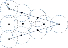
|
| Figure 39: Representation of a surface mesh size entity (a triangle) with a set of its generalized mesh size points (black dots). It can be seen that all the coordinates inside the triangle have at least one mesh size point closer than . |
It has to be noted that, following this definition, there can be infinite sets of generalized mesh size points. The process used to obtain them is detailed in Section 6.3.
The implementation of the mesh size entities criterion is simplified if the generalized mesh size points are considered instead of the mesh size entities.
5.2.2.3 Volume mesh sizes refinement criterion
For a given mesh size desired for each volume (considering as the desired size for the ith volume) the following criterion is defined:
RC 3: If an octree cell is an inner cell of the ith volume and its size is greater than , the cell must be subdivided.
5.2.2.4 Balance refinement criterion
The following refinement criterion is widely used in octree based meshers. It limits the number of neighbors of one cell, and it is often referred as constrained two to one condition (Section 3.3). It is an essential criterion for the pattern used for the creation of tetrahedra from the octree leaves:
RC 4: If an octree cell has more than four neighbor cells by face or two by edge, the cell must be subdivided.
5.2.2.5 Size transition refinement criterion
The balance criterion gives an upper limit for the size transition: as the size of two neighbor cells differs (at maximum) by a factor of 2, the difference between the size of the tetrahedra generated from those cells is bounded as well. However, it may be required for the final mesh to present a more smooth size transition between regions with small and large elements.
Considering the desired mesh size for given regions of the domain (from the input data), and a given size transition function, an envelope function can be defined to set an upper limit for the element size allowed in each position of the space . The definition if this function is detailed in Section 6.4, and leads to the following refinement criterion:
RC 5: Being the center of an octree cell, if the size of the cell is greater than , the cell must be subdivided.
5.2.3 Octree root
As explained in Section 3.2, the octree root is the bounding box of the octree. Clearly it should contain totally the domain to be meshed in its interior, but considering the meshing process, it has to accomplish some other requirements.
For the creation of the octree root, the extended bounding box of the model is needed (from now on ). is the minimum bounding box containing the bonding box of the model and all the generalized mesh size points. It has to be noted that the mesh size entities can be outside the domain. The octree root is built centered in the center of , and with a size equal to the maximum size of plus (Equation 5.2). This offset of the octree root with respect to is needed to ensure the tetrahedra creation by the tetrahedra pattern, considering that in some cases this creation involves one cell and its neighbor. A graphical 2D example (quadtree instead of octree) of the and the octree root is shown in Figure 40.
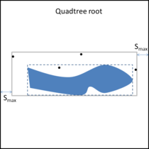
|
| Figure 40: 2D example where the domain is the solid surface. Black dots are the generalized mesh size points. The bounding box of the model is represented by the dotted line. The is the gray line, and the quadtree root is the black square. |
5.2.4 Meshing algorithm
Hereafter, the steps of the meshing algorithm for embedded meshes are presented.
- Process input data and create the octree root. This includes:
- Creation of generalized mesh size points (in case they exist).
- Compute .
- Creation of the octree root (Section 5.2.3).
- Refine the octree accomplishing the size refinement criteria (defined in Section 5.2.2):
- RC 1: Maximum size.
- RC 2: Mesh size entities.
- RC 3: Volume size.
- RC 4: Balance.
- RC 5: Sizes transition.
- Classify the input boundary entities into the octree. This step implies the identification of the octree leaves colliding with the input boundary. Until now the octree has been refined, but each one of the cells had no information about its type: interface, inner or outer. Prior to this step the input boundaries only have been taken into account for building the bounding box of the model. At this point is where the input boundaries (surface entities from the input data) are analyzed in order to determine the interface cells. Furthermore (as it will be explained in Section 6.2) in the implemented octree, each interface cell stores the input boundary entities colliding with it.
- Create and color the linear octree nodes (Section 3.3.2) and compute the distances to the input boundaries (Section 5.2.1).
- Apply the tetrahedra pattern.(Section 3.3.3).
A 2D example of the algorithm is depicted in Table 5.2.4, where each step is illustrated by a figure. The model is formed by two surfaces in contact (drawn in orange and blue), and it contains only two mesh size points (represented by a cross in the figures) in the input data.
| 1- Process input data and create the octree root. The crosses are the mesh size points. The arrow beside each mesh size point represents its associated size. The octree root is the black square, and the of the model is drawn with dotted lines. in this example coincides with , as it is the largest size coming from the generalized mesh size points, and it is smaller than . | 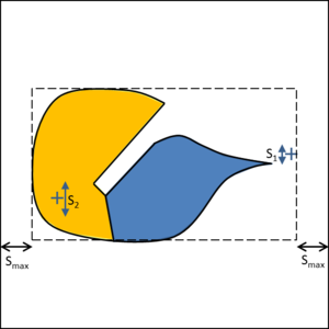
|
| 2- Refine the octree accomplishing the size refinement criteria. In this example the size transition factor is equal to one (the transition corresponds to the constrained two to one condition) to make the figure clearer. | 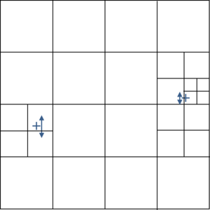
|
| 3- Classify the input boundary entities into the octree. It is important to note that, until now, the input boundaries only have been considered to build the bounding box of the model, but they have not been implied in the octree refinement process. | 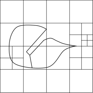
|
| 4- Create and color the linear octree nodes and compute the distances to the input boundaries. The nodes of the figure are painted with the corresponding color: orange or blue if they are inside the corresponding surface, black if they are onto the input boundaries, and white if the are outside the domain. | 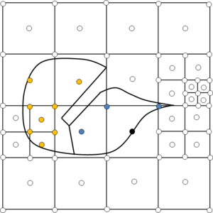
|
| 5- Apply the tetrahedra pattern. It can be appreciated in this figure that the final tetrahedra (triangles in this 2D case) are not body-fitted, as they do not preserve the original shape of the domain. | 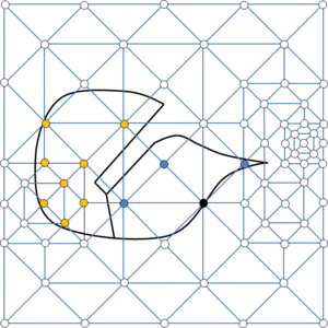
|
Steps followed by the embedded meshing algorithm applied to a 2D example with two surfaces and two mesh size points.
5.3 Body-fitted mesher
The concept of body-fitted mesh is applied to a mesh which contours represent precisely the shape of the contours of the domain. Considering the presented algorithm is a volume mesher generating a body-fitted mesh implies, from the geometrical point of view, that the final tetrahedra mesh must take into account lower level entities: point, line and surface ones.
The adaptation of the final mesh to the surface entities defining the different volumes of the domain plays a key role to ensure the preservation of the topology of the model and the accuracy of the mesh near the contours. This process is detailed in Section 5.3.6.
In the literature, the concept of geometrical features is used to refer the point and line entities relevant for the shape definition of the model, which must be preserved in the final tetrahedra mesh. Point entities to be preserved are the ones where the surface normal has multiple discontinuities and are referred as corners. Line entities to be preserved are the ones shared by two surfaces forming a sharp angle in it and are referred as ridges.
An example of two meshes of the same model (one preserving and the other one not preserving the geometrical features) is shown in Figure 41.
|
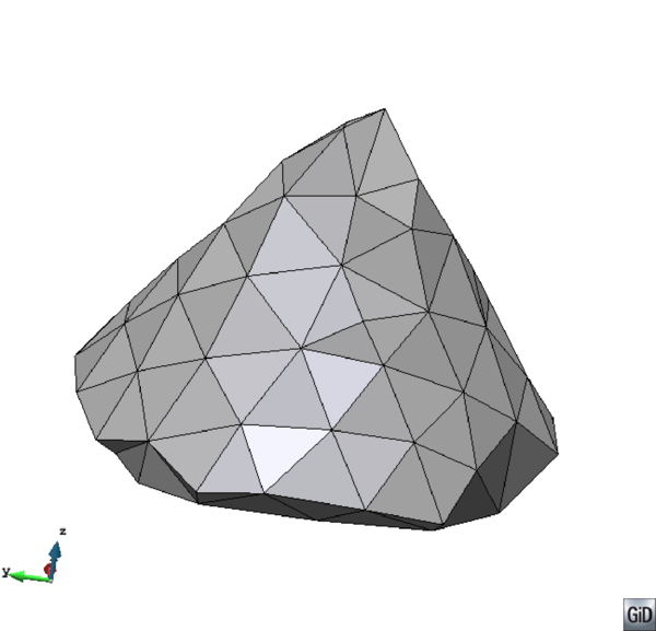
|
| (a) Geometrical model. | (b) Non body-fitted mesh. |

| |
| (c) Body-fitted mesh. | |
| Figure 41: Example of body-fitted and non body-fitted mesh of a geometrical model of a cone. The non body-fitted mesh does not preserve the apex of the cone (corner), nor the line entities (ridges) defining its base. | |
The preservation of the geometrical features is one of the weak points of the octree-based meshers. As these family of meshers are based in a regular grid (the octree) rather than in the shape of the domain, when the shape of the domain has specific distorted regions in comparison with the octree cells, some strategy has to be followed. One can think that refining the octree in those regions should solve the problem, but this is not true, as some configurations can lead to an infinite refinement process. This is because the geometrical problems governed by angles are reproduced exactly in all the refinement levels.
In this work, not only the geometrical features are taken into account to be preserved in the final mesh, but also forced point and forced line entities coming from the input data, needed to preserve the topology of the model or to provide with specific attached data to the final mesh entities. The generalized concept of forced edges and forced nodes (detailed in Sections 5.3.1 and 5.3.2) is used to include all the line and point entities to be preserved, independently on its purpose: preservation of topology or preservation of geometrical features.
5.3.1 Forced edges
In case the input data for the mesher has forced line entities (from the input data), or a minimum angle for sharp edges is defined, the so called forced edges must be created. These are edges the final tetrahedra mesh will preserve. Forced edges plays a key role for preserving sharp edges and representative surface and line topology.
| ||||||
| Figure 42: (a) Contours of a volume with some of its sharp edges highlighted. (b) Constrained tetrahedra mesh of the volume highlighting the sharp edges corresponding to the ones in figure (a).(c) Partially constrained tetrahedra mesh of the volume highlighting the sharp edges corresponding to the ones in figure (a). |
At this point it has to be noted that the mesher is partially constrained. In this context, the term partially constrained means that if there are some forced line entities to be preserved, a collection of edges from the final mesh should follow the path of those line entities. This is not as restrictive as totally constrained condition, which would force to have as much edges in the final mesh as the number of forced line entities, and bounded (each one of the edge) by the same nodes bounding the forced line entities.
This difference can be appreciated in the Figure 42, where the definition of a domain is shown with some of its sharp edges highlighted (Figure 42(a)), and two different final meshes of the domain being partially or totally constrained are shown. In this example forced edges come only from the sharp edges of the domain. As it can be seen in Figure 42(b), generating a totally constrained mesh yields a mesh with the same sharp edges present in the input data. In Figure 42(c) it can be appreciated that a different number of edges are generated to represent the initial forced edges: generating a partially constrained mesh, a collection of sharp edges follows the path of the sharp edges present in the input data, so as the shape of the domain to be meshed is well captured.
The creation of the forced edges is based on three steps: identification of the base line entities, creation of the polyline entities and linear mesh generation from the polyline entities:
- Identification of the base line entities. The base line entities are line entities coming from three different sources:
- Forced line entities: each forced line entity from the input data is directly a base line entity.
- Line entities shared by more than two surface entities from the input boundaries. A T-junction is an example of this case, where a line entity is shared by three surface entities.
- Line entities shared by two surface entities from input boundaries which form an angle (along the line entity) smaller than the maximum angle for sharp edges (in case it is defined in the input data). The angle between two surface entities is not well defined, as it can only be evaluated point by point. In the present work, the angle between two surface entities along their common line entity is defined as the mean of the angles formed by the normal vectors of each surface entity in some sampled points of the line entity. The number of points used depends on the curvature of the surface and line entities.
- Creation of the polyline entities. In this step, the collection of base line entities is clustered in different groups called polyline entities in such a way that two base line entities are in the same polyline if:
- they share a point entity,
- and the shared point entity does not belong to any other base line entity,
- and the angle formed by the tangent vectors of each line entity in the shared point is smaller than the maximum angle for sharp edges.
- Generate a mesh from the polyline entities. In this step a linear mesh is generated from each polyline entity taking into account three criteria for the linear element creation:
- If a polyline entity is closed (both extreme nodes are the same one), it must have at least three elements. This condition avoid the creation of zero-volume elements in the final mesh.
- If the base line entities forming the polyline entity has some desired size assigned (from the input data), a desired size can be computed for each linear element. This is the mean of the desired sizes of the base line entities in the positions of the nodes of the element. Each element of the mesh must have a length equal or lower than its .
- The chordal error of the elements of each polyline meshes is limited by the most restrictive value between the chordal error required by the simulation (in case it is defined in the input data) and a given relative chordal error . The relative chordal error is defined as the chordal error of the element divided by its length. The parameter tries to ensure that the forced edges describe correctly the shape of the forced line entities and the input boundaries. The value of this parameter is discussed in Section 6.7.
Note that the base line entities is a collection of line entities in the space, and they can be related or not to the input boundaries of the domain.
In case of non watertight input boundaries, a previous collapse of nodes and edges may be done to the input boundaries in order to be able to capture the sharp edges, as two surface entities forming a sharp edge may not be in contact topologically. This aspect is treated later on.
The result of this clustering operation leads to a collection of polyline entities having each one of them one or more base line entities. Two point entities can be identified as extremes of each polyline entity.
The polyline entities corresponding to the base line entities shown in Figure 43(a) are depicted in Figure 43(b). In this example base line entities and are not part of the same polyline entity because they form a small angle in the common point (smaller than an hypothetical maximum angle for sharp edges).
| ||||||
| Figure 43: Example illustrating the entities involved in the creation of the forced edges. (a) A collection of base line entities , , , , , , , and . (b) The polyline entities , , , and created from the base line entities shown in Figure (a) considering the angle between and smaller than the maximum angle for sharp edges (from in input data). (c) A possible distribution of forced edges (shown in dotted line) created from the polylines present in Figure (b). |
The discretization of the polyline entities can be done using any mesh generation method. This linear mesh will be used only auxiliary (it will not be part of the final mesh) and its quality is not relevant more than providing a sort of sizes distribution in the octree. In this work a simple recursive splitting method is used to generate the mesh of each polyline entity. The method creates one linear element using the two extreme nodes of the polyline entity, and subdivide it recursively until all the elements accomplish with the three criteria defined above. It has to be considered that each new edge node created when an element is subdivided is mapped onto the polyline entity in order to capture well the shape of it.
The forced edges are directly the elements of the meshes generated from the polyline entities.
Note that the two first steps refer to line entities in general, without specifying if they are CAD or mesh entities. The forced edges created in the third step are always mesh entities.
For notation purposes, the extreme nodes of a forced edge are called edge nodes. Each forced edge has two (and only two) edge nodes, and each edge node can belong to more than one forced edge.
It will be seen later on that the octree cells near a forced edge should have a similar size to it not to produce too distorted tetrahedra. To reach this goal, the forced edge condition has been defined:
Forced Edge ConditionForced Edge Condition
Condition 1: Being cell A the octree leaf containing one edge node of a forced edge, and cell B the octree leaf containing the other edge node of the forced edge, the degree of neighborhood between A and B must be lower or equal than two.
Considering a given configuration of the octree, all the forced edges must accomplish the Forced Edge Condition. If a forced edge violates it, it must be subdivided in other forced edges until all of them accomplish it. The split of the edge is done by its middle point. It has to be taken into account that the subdivision of a forced edge implies the creation of new edge nodes. These ones are mapped onto the polyline entity where the forced edge comes from to yield a better approximation of the shape.
5.3.1.1 Pathological configurations of forced edges
There are some pathological situations for forced edges that can occur due to given configurations of input boundaries:
- Very thin surface entities. The presence of very thin surface entities in the boundary may be a problem due to the distortion in the computation of their normal vector. In case of triangles, the normal vector is computed using the vector product of two of their adjacent sides. If one of the them is very small (almost zero), the normal vector calculated becomes erroneous: it can point to any direction. For this reason, when comparing normal vectors of adjacent triangles in order to set sharp line entities, some fake ones may be detected.
- Very close forced line entities. The presence of very near forced line entities without intersection may lead to very distorted elements in the final mesh. Furthermore, some of the octree refinement criteria (Section 5.3.3) may lead to infinite level of refinement in this situations.
A possible strategy to solve the first situation is to collapse the line entities with a length lower than a given tolerance, or directly exclude these small ones as forced line entities. Collapsing the small line entities may not solve the problem, because they may belong to a longer polyline entity (also fake) which won't be collapsed. The option of not considering the small line entities also may fail, because there may be some cases where a relevant polyline entity is formed by very small line entities.
For the second situation, a possible solution may be to collapse the line entities which are close enough one from each other. However, these geometrical operations are not trivial in some 3D configurations.
In order to detect the sharp line entities, only the ones belonging to two, and only two, surface entities are considered. Cases where more than two surface entities share a line may be important for the topological definition of the domain. In these cases, the corresponding line entity should be set as forced line entity in the input data, not in the sharp edges detection process. The edges surrounding a gap (in case of non-watertight boundaries) are not considered to be preserved.
These automatic strategies may not solve all the pathological situations that can occur in the input boundaries. Hence, it may be needed to preprocess them in order to specify the desired forced line entities following given criteria to accomplish the simulation requirements. This is the case of the example shown in Figure 44. The input boundaries of this example are depicted in Figure 44(a). As it can be seen, there are very thin triangles. The normal vector of these triangles is not well computed numerically. When comparing the normal vector of two adjacent triangles, some edges which are not sharp are detected as so. It is the case of the small edges depicted in Figure 44(b).
| ||||||
| Figure 44: (a) Input boundaries (triangles) of a part of an example model of a mechanical piece. (b) Zoom view of Figure (a), where the shape is smooth enough not to present sharp edges. (c) Same view of (b), showing only the sharp line entities (black lines) automatically detected considering the normal vectors of the triangles of the boundaries (dotted lines surround them in order to highlight their position). As there are very thin triangles, some normal is not well computed, so some of the detected sharp line entities are fake. |
In this example, some of the fake sharp edges (forced line entities) are connected creating the corresponding polyline entity. These polyline entities are not so small, so collapsing the nodes of the small forced line entities will not eliminate these fake ridges: the polyline entity would remain, but with less forced line entities. A possible solution here is to consider only the polyline entities longer than a given tolerance (as the polyline entities useful to define the shape of the domain are much more longer). However, this strategy cannot be applied in general. Some models may not have a so clear separation between the lengths of relevant and not relevant sharp entities.
In cases where the 3D model is not very complex, another option could be to select manually a priori the line entities to be forced ones.
In conclusion: Depending on the quality of the input boundaries of the domain, more information may be needed in order to identify clearly the forced line entities to be preserved by the mesher. In these cases, the geometrical definition of the domain is not enough to set the appropriate forced edges.
5.3.2 Forced nodes
The forced nodes are octree nodes (linked to an octree position) with a prescribed position in space: the forced position. The forced position of a forced node is not coincident with the octree position it is linked to. There are three kinds of forced nodes:
- Forced isolated nodes. These ones are created directly from the forced point entities given by the input data. Every forced point entity becomes a forced isolated node whose forced position is the one of the forced point entity and the related octree position is the closest one to it.
- Forced nodes in edge. These forced nodes correspond to the edge nodes (Section 5.3.1). Every edge node become a forced node in edge which forced position is the one of the edge node and the related octree position is the closest one to it.
- Forced interface nodes. These correspond to octree nodes which octree position is very near to the input boundaries. Taking into account an octree node, lets define as its closest coordinate onto the input boundaries. Considering the distance from an existing octree node to its , and the size of the octree leaf the octree node is into, an octree node is a forced interface node if
|
|
(5.3) |
where is a real positive value. The value of must be lower than , otherwise it could lead to inverted tetrahedra (with negative jacobian) when applying the tetrahedra pattern (Section 3.3.3). The tuning of this value is explained in Section 6.7.
The forced position of a forced interface node is the of the octree node it is generated from. It is important to note that the definition of the forced interface nodes depends on the size of the octree cells, so an octree node can be considered as a forced interface node or not depending on the size of the cells surrounding it. It can be seen that refining an octree can lead to the creation or deletion of some forced interface node.
It will be seen in Section 5.3.3 that the forced nodes are involved in an octree refinement criterion (RC 6). To anticipate the general idea, each forced node is linked to an octree position, and each octree position cannot have more than one forced node associated. So if two forced nodes are very close one from each other, the octree cell containing them should have a size similar to the distance between them. This could lead to an excessive level of refinement of the octree, specially in cases where there are non-watertight definitions of the boundaries.
In extreme cases where the forced nodes can be almost exactly in the same position, the refinement criteria could lead to an infinite level of refinement. To solve this problem, the forced nodes which are closer than a given tolerance (a portion of the mesh desired size) are collapsed. It has to be considered that if two forced nodes are collapsed and they belong to a forced edge, it must be collapsed as well.
5.3.3 Octree refinement criteria for body-fitted meshes
All the size refinement criteria (the ones applied for embedded meshes, detailed in Section 5.2.2) are also applicable to body-fitted meshes, as they are based on the desired mesh size.
In this section the specific refinement criteria (RC) needed for body-fitted meshes are defined. Some of them may not be applied in the meshing process depending on the input parameters.
These refinement criteria are a key point for the body-fitted mesher, as they ensure the geometrical features of the domain and its topology will be preserved by the tetrahedra generated from the octree.
5.3.3.1 Forced nodes refinement criterion
The following criterion refers to the forced nodes. As it has been explained in Section 5.3.2, each forced node is associated to an octree cell position.
RC 6: If an octree cell has a forced node inside, and the octree position associated to that forced node is occupied by another forced node, the cell must be subdivided.
In order to ensure that this refinement criterion does not lead to an infinite level of refinement, the distance between forced nodes must be greater than a minimum value, corresponding to the minimum cell size allowed in the octree. The fulfillment of this condition involves a treatment of the forced nodes before the refinement criterion: if two forced nodes are closer than the minimum cell size allowed in the octree they are collapsed into one. If they are part of a forced edge, the forced edge is also collapsed.
5.3.3.2 Tetrahedra distortion refinement criterion
For the refinement criteria defined hereafter, the tetrahedra created from the octree following the tetrahedra pattern are considered. For this reason, these criteria only take sense if the RC 4(balance) and RC 6(forced nodes) are accomplished. From now on the concept of the tetrahedra created from an octree cell is used to refer the tetrahedra result from applying to the cell the patterns defined in Section 3.3.3.
The quality of the tetrahedra generated from cells without forced nodes is very high (and it can be evaluated a priori), but the presence of forced nodes implies that their positions in space are not the octree positions, so the tetrahedra generated may be distorted.
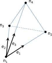
|
| Figure 45: Tetrahedron with the local node numeration following the right hand rule. Vectors involved in the definition of an inverted tetrahedron are depicted. |
The concept of inverted tetrahedron must be defined at this point in order to introduce the following refinement criterion. Considering a tetrahedron with its nodes , , and sorted in a given way (as the tetrahedron depicted in Figure 45), it is inverted if the scalar product of x by is negative. , , and are vectors aligned with the directions , and respectively, oriented from towards the other nodes. In the case where the scalar product is null, the tetrahedron has zero volume and receives the name of sliver.
RC 7: If a tetrahedron created from an octree cell is inverted or a sliver, the cell must be subdivided.
5.3.3.3 Topological refinement criterion
The following refinement criteria are the basis to ensure the preservation of the topology for the mesher. Some auxiliary definitions are needed here. If we consider an edge of a tetrahedra generated from a cell, a limit distance of the edge is defined as
|
|
(5.4) |
where is the length of the edge and is a real value between zero and one (the value taken for this parameter is detailed in Section 6.7).
The so called intersection points of an edge are the intersection points between the edge and the input boundaries. As an intersection operation between an edge and surface entities, the following situations must be considered (see also Section 3.4):
- If the intersection between an edge and the the surface entity defining the input boundaries is co-planar ( intersection type), any intersection point is considered.
- For the evaluation of the following refinement criterion, a is created only if all the intersected surface entities involved interface the same volumes.
- As the extremes of an edge are already colored, if both belong to different volumes and no intersection point has been detected, the corresponding must be considered as the intersection point.
If we define the portion of a given volume enclosed in an octree cell delimited by the input boundaries and the cell faces, the interface cells can have several portions of volumes. Let us name face limit surfaces to the boundaries of these portions of volumes laying onto the the cell faces. An example of the portions of volumes of a cell is shown in Figure 46.
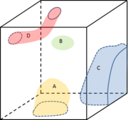
|
| Figure 46: Example of portions of volumes enclosed in an octree cell. Volume lies onto one face of the cell creating one face limit surface, volume does not lay onto any face of the cell, volume lies onto three faces of the cell creating three connected face limit surfaces, and volume lies onto two faces of the cell creating two unconnected face limit surfaces. |
RC 8: This criterion is split in three levels:
- 8(a) If an edge of a tetrahedra created from an octree cell fulfill some of these conditions:
- both extreme nodes of the edge are forced nodes and there are more than one intersection point,
- one extreme node of the edge is a forced node and the distance between it and an intersection point is lower than ,
- there are two intersection points and the distance between them is lower than , or
- there are more than two intersection points,
then the cell must be subdivided.
- 8(b) If a portion of volume enclosed in an octree cell does not intersect any edge from the tetrahedra created from the cell, and it lies onto more than one face of a cell creating unconnected face limit surfaces, then the cell must be subdivided.
- 8(c) If a portion of volume enclosed in an octree cell does not lay onto any face of the cell and does not intersect any edge from the tetrahedra created from the cell, then the cell must be subdivided.
The implementation of these refinement criteria is detailed in Section 6.5.
Examples of different configurations of an edge fulfilling the refinement criterion 8(a) are shown in Figure 47.

|

|
| (a) | (b) |

|

|
| (c) | (d) |
| Figure 47: Different configurations of the edge that force the refinement of the octree in order to accomplish the refinement criterion 8(a). Dotted line represents the input boundaries and crosses are the intersection points between the edge and the input boundaries. (a) Both and nodes are forced nodes and there are more than one intersection point. (b) is a forced node ( could be forced node or not), and there is an intersection point closer than to it. (c) there are two intersection points and the distance between them is lower than . (d) There are more than two intersection points. | |
An example of a pathological configuration where the refinement criterion 8(b) is needed is the portion of volume of Figure 46. On the other hand, the portion of volume of the same figure evidences the need for the fulfillment of the criterion 8(c) in order to preserve the topology of the input data.
5.3.4 Meshing algorithm
Hereafter, the steps of the meshing algorithm for body-fitted meshes are presented:
- Process input data and create the octree root.
- Creation of forced edges and forced nodes (in case they exist).
- Creation of generalized mesh size points (in case they exist).
- Compute .
- Creation of the octree root. The creation of the octree root is done in the same way as for embedded mesher (Section 5.2.3).
- Refine the octree according to the size refinement criteria (the ones used for the embedded mesher, defined in Section 5.2.2).
- Classify the input boundary entities into the octree. Here is where the input boundaries (surface entities from the input data) are analyzed in order to determine the interface cells. Before this step the input boundaries only have been taken into account for building the bounding box of the model.
- Color the octree nodes (Section 4) and detect the forced interface nodes.
- Refine the octree to fulfill the specific criteria for body-fitted meshes (defined in Section 5.3.3):
- RC 6: Forced nodes. This implies enter the forced nodes into the octree, which is assign an octree position to each one of them.
- RC 7: Tetrahedra distortion. (See page current).
- RC 8: Topology. (See page current).
- Apply tetrahedra pattern (Section 3.3.3). In this step, for all the interface and inner cells (not the outer ones) the tetrahedra are created following the tetrahedra patterns.
- Preserve geometrical features (Section 5.3.5). After this step all the forced edges are edges of the tetrahedra mesh, and the octree nodes linked to a forced node have been placed in the corresponding position.
- Apply surface fitting algorithm (Section 5.3.6). Some nodes are placed onto the surface entities defining the contours of the volumes, and some tetrahedra may be split.
- Color tetrahedra and create skin triangles of volumes (Section 5.3.7). After this step all the tetrahedra can be assigned to a specific volume or the outer part of the domain. Now the tetrahedra and the nodes of the outer part of the domain can be deleted. The skin triangles of the volumes is formed by the faces (triangles) between tetrahedra of different color, or interfacing a tetrahedron with the outer part of the domain.
- Make-up and smoothing. This step can be considered out of the mesh generation algorithm itself, as it consists in the improvement of the quality of the elements generated, and it can be applied to any tetrahedra mesh. However, it is highly necessary considering the quality of the tetrahedra in the contours of the domain (Section 5.3.8).
This step implies the coloring of the appearing octree nodes. RC 4 (balance) has to be also taken into account during this refinement process, as it is mandatory for the tetrahedra generation following the given patterns.
From now on, the octree structure is frozen in the sense that its cells will not be refined any more.
Note that the refinement process involved in the fifth step is an iterative process. Every time an octree cell is subdivided, several aspects have to be considered in the new configuration of the octree:
- New octree nodes are created, so they have to be colored.
- Some of the new octree nodes may be forced interface nodes.
- Some previously existing forced interface nodes may become regular nodes (not forced ones).
- Some forced edge may be subdivided in order to accomplish the maximum Forced Edge Condition(Section 5.3.1).
- New forced nodes (interface or edge ones) may be created.
All this aspects may force the subdivision of other cells due to the other refinement criteria, so an iterative process is required in order to achieve an octree configuration where all the refinement criteria are accomplished. However, in our experience, few iterations are enough for satisfying all of them. The implementation of the algorithm is detailed in Section 6.5.
Another important characteristic of the algorithm is that the first six steps are based on the octree, while from the seventh step onwards, the operations are applied to the unstructured tetrahedra mesh.
A graphical example of the steps of the meshing process is shown in Table 5.3.4 using a 2D model to make the figures more understandable. In the first figure, the offset between and the octree root should be equal to , but it has been put smaller to make the following figures clearer.
It also has to be considered that some of the parts of the algorithm are intrinsically 3D (such as the process to preserve forced edges), so they cannot be illustrated with a 2D model. This example is formed by two surfaces and it has no mesh size information in the input data. It is important to note the presented algorithm is able to generate a body-fitted mesh with the only information of the input boundaries.
| 1- Process input data and create the octree root. The red small squares represent forced points. The octree root is the black square, and the of the model is represented with dotted lines. In this example coincides with the minimum side of the model bounding box (), as there are no mesh size points. | 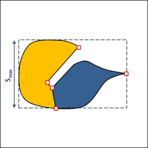
|
| 2- Refine the octree accomplishing the size refinement criteria. As there are no mesh size point in the model, the octree is refined uniformly with . | 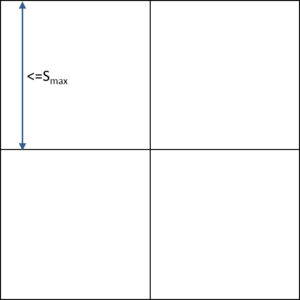
|
| 3- Classify the input boundary entities into the octree. It is important to note that until now, the input boundaries only have been considered to build the bounding box of the model, but they have not been implied in the octree refinement process. | 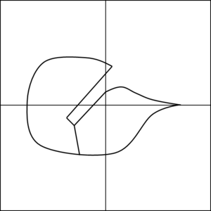
|
| 4- Color the octree nodes and set forced interface points. The nodes of the figure are painted with the corresponding color: orange or blue if they are inside the corresponding surface, black if they are close enough to the contour entities to be forced interface nodes. Nodes outside the domain are white. | 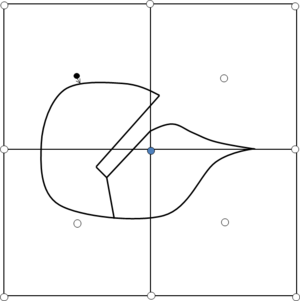
|
| 5- Refine the octree according with the body-fitted refinement criteria. It can be appreciated that the octree refinement process leads to the creation of new octree nodes. Some of them become forced isolated nodes (red ones) or forced interface nodes (black ones). The arrows indicates the forced position of each forced node. | 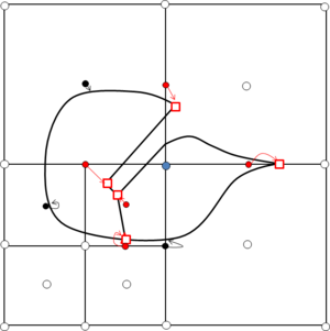
|
| 6- Apply the tetrahedra pattern. The tetrahedra are generated from the octree nodes. From this step on, the operations are performed to the corresponding tetrahedra mesh rather than the octree one. | 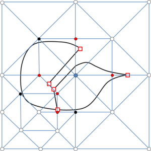
|
| 7- Preserve geometric features. At this point forced nodes are moved into their forced positions. As a 2D example, only the moving of forced nodes can be appreciated in the figure (the preservation of edges has no sense in 2D). | 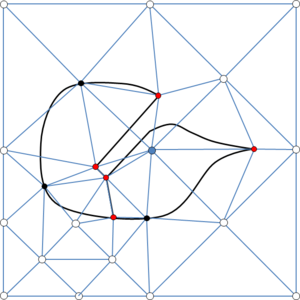
|
| 8- Surface fitting process. This is the last step of the process which ensures the final mesh could represent the original topology of the input boundaries. | 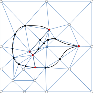
|
| 9- Tetrahedra coloring and identification of skin mesh. Elements owning to the orange or blue surface are painted accordingly in the figure. After this process the outer elements can be deleted. | 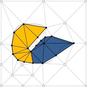
|
| 10- Make-up and smoothing. In this step some mesh editing operations are done in order to improve the mesh quality. | 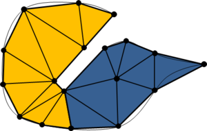
|
Steps followed by the body-fitted meshing algorithm applied to a 2D example with two surfaces with no mesh size assigned.
5.3.5 Preserve geometric features
The preservation of geometrical features (corners and ridges) lies on the preservation of forced nodes (Section 5.3.2) and forced edges (Section 5.3.1).
The operations described in this section are performed after the creation of tetrahedra from the octree leaves following the tetrahedra pattern (Section 3.3.3), so at this point there are forced nodes, forced edges and a tetrahedra mesh got directly from the octree cells. This tetrahedra mesh covers the domain to be meshed, but does not preserve the geometrical features and does not fit the surface entities representing the interfaces between volumes (there are nodes outside the domain and tetrahedra with edges crossing volume interfaces). The aim of this process is that the tetrahedra mesh has nodes in the corresponding positions of the forced nodes, and edges corresponding to the forced edges.
Each forced node has an octree node associated to it. The process of preserving the forced nodes is reduced to move the corresponding octree nodes to the position of its forced node.

|

|
| (a) | (b) |
| Figure 48: Process of splitting a forced edge by inserting a node onto its base line. (a) Forced edge to be split by the node ; the dotted line is the base line of the forced edge. (b) Forced edges and result from splitting the forced edge by the node ; dotted lines are the corresponding base lines of the forced edges. | |
Concerning forced edges, the goal is to force the tetrahedra mesh to have edges coincident with them. As explained in Section 5.3.1, the forced edges are obtained as a linear mesh from the polyline entities. The portion of polyline entity enclosed between the extreme nodes of a forced edge can be defined as the base line of the forced edge. Note that this is a pure notation, as the polyline is made of generic line entities (in mesh or geometrical format). For notation purposes, a forced edge will be defined by its extreme nodes: the forced edge is the one which extreme nodes are node and node . The same notation is used for a generic edge of a tetrahedron.
From now on the concept of fitting the tetrahedra mesh to the forced edges is used to define the process of having an edge of the tetrahedra mesh for each forced edge. To achieve this goal a splitting process of forced edges and tetrahedra is proposed. This process involves three basic operations:
- Split a forced edge by inserting a node onto its base line. This process is shown in Figure 48 and it creates two forced edges from an original one connecting its extreme nodes with the splitting node. The base line of the forced edge is split by the node as well.
- Split an edge of a tetrahedron. This process involves all the tetrahedra surrounding the edge. Each of them is split into two tetrahedra as shown in Figure 49(b).
- Split a face of a tetrahedron. This process involves a tetrahedron and the neighbor to the face. Each of these two tetrahedra generate three tetrahedra as shown in Figure 49(d).
| ||||||||
| Figure 49: Process of splitting tetrahedra by a node. (a) Edge to be split by the node , with its surrounding tetrahedra around (4 in this example). (b) 8 tetrahedra result from splitting the edge by the node . (c) Face to be split by the node , with the two tetrahedra sharing the face. (d) 6 tetrahedra result from splitting the face by the node . |
Hereafter the process needed for fitting the tetrahedra mesh to the forced edges is detailed. For each forced edge we check whether nodes and are nodes of a same tetrahedra or not. In case they are, the tetrahedra mesh has an edge coincident with the forced edge, so the objective is already achieved. In case there is no tetrahedra containing nodes and , the following procedure must be considered (a graphical example of the steps followed to fit the tetrahedra mesh with a forced edge is shown in Table 5.3.5):
- Find the tetrahedron surrounding node which opposite face with respect to (from now on ) is intersected by the base line of the forced edge. Note that the base line can be represented by geometrical or mesh entities (NURBS curve or linear mesh). In case of a linear mesh, the intersection operation between the base line and the faces of tetrahedra is much more robust and computationally cheaper.
- Find the intersection point between the base line and . Defining as the length of the shortest edge of , a node () is created taking care on the following casuistic (a graphical view of the entities involved is shown in Figure 50):
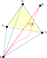
|
| Figure 50: Entities involved in the process of making the tetrahedra mesh to have an edge coincident with a forced edge. Red line is the forced edge and the dotted red line is its base line. The tetrahedron is the tetrahedron surrounding node which opposite face with respect to () is intersected by the base line. Face is the (drawn in yellow). is the intersection point between the base line and . The closest node of to is , and the closest edge from to is the edge . |
- If the distance between and its closest node of is lower than (), then this node is moved to the position of and it is considered as the node . The parameter is a real value between zero and one; the value used for it in the presented implementation of the algorithm is discussed in Section 6.7. This is the case shown in figures d) and e) of Table 5.3.5.
- If the previous case is not accomplished and the distance between and its closest edge of is lower than (), node is created in the position of , and the closest edge is split by the node . The parameter is a real value between zero and one; the value used for it in the presented algorithm is discussed in section 6.7. This is the case shown in figures f) and g) of Table 5.3.5.
- If the previous cases are not accomplished, node is created in the position of and is split by the node . This is the case shown in figures b) and c) of Table 5.3.5.
- Split the forced edge by the node . Now the forced edge is an edge of the tetrahedra mesh.
- If the forced edge is not an edge of the tetrahedra mesh, repeat the process with it.
Note that the nodes created in this process are not octree nodes, as they are not related with any octree position. Furthermore, these nodes do not need any coloring algorithm, as they lay on a interface entity.
| (a) Initial configuration of the forced edge (red line) with its surrounding tetrahedra (in blue), and its base line (dotted red curved line). | 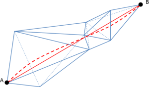
|
| (b) Find the tetrahedra () owning node which opposite face to it () intersects the base line of forced edge . is the intersection point. | 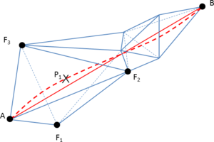
|
| (c) As is not close enough to , or , and neither to the edges of face , create the node in the position of and split the face and the forced edge by the node . Now the forced edge is already an edge of the tetrahedra mesh. | 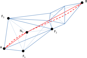
|
| (d) Proceed the treatment of forced edge . Find the tetrahedra () owning node which opposite face to it () intersects the base line of forced edge. is the intersection point. | 
|
| (e) As is close enough to (closer than times the minimum edge of ), move to the position of and split forced edge by node . Now the forced edge is already an edge of the mesh. | 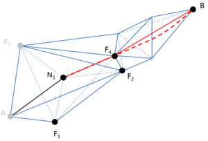
|
| (f) Proceed the treatment of forced edge . Find the tetrahedra () owning node which opposite face to it () intersects the base line of forced edge. is the intersection point. | 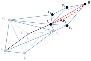
|
| (g) As is close enough to edge (closer than times the minimum edge of ), creation of node in the position of and split of edge and the forced edge by the node . Now the forced edges and are edges of the mesh, so the process is finished. | 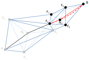
|
| (h) Final configuration of the tetrahedra with the new forced edges created: , , and . | 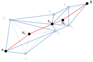
|
Example of the process to fit a tetrahedral mesh with the forced edge .
5.3.6 Surface fitting
This section describes the process of fitting the tetrahedra mesh into the volumes of the domain to be meshed, representing their interface surfaces accurately (from now on surface fitting process). The methodology presented is applied to the tetrahedra mesh (come from the tetrahedra pattern defined in Section 3.3.3), in which the process of preserving geometrical features (defined in Section 5.3.5) has been carried out. Some of the nodes of the mesh are forced nodes (fixed in a position in space) and some of its edges are coincident with the forced edges. The process defined from now on preserves the forced nodes as well as the edges corresponding to the forced edges.
The surface fitting process is based on the isosurface stuffing method published in [37] (from now on isostuffing method). However, it has some differences, as its objectives and restrictions are different:
- The isostuffing method is applied to an isolated volume. In this work all the volumes of the domain are meshed together, and they can be in contact one to each other.
- The isostuffing method do not preserve sharp edges nor corners. The present algorithm must respect the forced nodes and forced edges in order to preserve the topology of the model and its geometrical features.
- The isostuffing method does not preserve the topology of the domain, as the size of the cells used is chosen by the user a priori; if this size is much more greater than a thin part of the domain, this part will not be represented by the final mesh. The surface fitting process presented in this work ensures the topology of the mesh will be the same as the one of the input geometry. This is due to the topological refinement criteria applied to the octree the mesh is generated from.
An example of tetrahedra mesh generated using the isostuffing method is shown in Figure 51. It can be appreciated that the sharp edges relevant for the definition of the shape of the model are not preserved by the mesher.

|
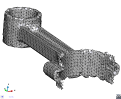
|
| (a) | (b) |
| Figure 51: Example of a 3D model of a mechanical piece (a) and a tetrahedra mesh of it generated using the isostuffing method (b). | |
The surface fitting process is based on the edges of the tetrahedra mesh which are not forced edges: the iso-edges. It consists in the following steps:
- Compute iso-edges intersections. Compute the intersection of the iso-edges with the input boundaries (intersection points). As described in Section 3.4, the following situations must be considered:
- If the intersection between an edge and the the surface entity is co-planar ( intersection type), no intersection point is considered.
- Intersection points closer than are collapsed into a .
- As the extremes of an edge are already colored, if both belong to different volumes and no intersection point has been detected, the corresponding must be considered as the intersection point.
- Move nodes. For each node of the iso-edges, we consider its closest intersection point (between the intersection points of the edges containing the node). It can be assigned to each of these nodes () the closest intersection point () and the edge the is into (). Then, if is not a forced node, move it to the position of if
- Split edges. Split the remaining iso-edges (the ones with intersection point after the node moving process) by their intersection point reconnecting the surrounding tetrahedra, as shown in Figures 49(a) and (b).
- Repeat steps 1, 2 and 3 with a new set of iso-edges: the ones of the mesh having at least one if its nodes onto the input boundaries.
- Repeat steps 1, 2 and 3 with a new set of iso-edges: the ones of the mesh fulfilling the following conditions (both of them):
- At least one of the nodes of the edge is onto the input boundaries.
- At least one of the nodes of the edge is connected (by an edge) to a forced node in edge.
Some of the edges can intersect more than one time the input boundaries, but not more than two due to the topology criterion (a). In these cases with two intersections only one of them is taken into account (no matter which one). From now on we only take care of the edges intersecting the input boundaries; the ones that do not intersect them are taken out from the iso-edges.
|
|
where the distance between and , and the length of the edge . The parameter is a real value between zero and one. The value used in the algorithm is explained in Section 6.7. This process of moving the node is only performed if the resulting configuration does not generate poor quality tetrahedra.
Moving a node implies to recompute the possible intersection points of all its connected edges, as one of their extremes is moved. This leads to an iterative process where new edges can be added to the iso-edges, and some existing one can be taken out (the ones with no intersection point). A 2D example of a situation where the movement of a node creates a new intersection point is shown in Figure 52.
|
|
| (a) | (b) |
| Figure 52: 2D example of creation of a new intersection point when moving a node. Black line represents the input boundaries, and part of the triangle mesh is shown in blue. (a) Initial configuration: node is close enough to intersection point , so it is moved. (b) Final configuration after moving : the new intersection point has appeared. | |
| |
| (a) Initial configuration of the mesh before surface fitting process. | (b) Detection of the intersection points (red dots). Nodes and are close enough to its closest intersection points (red circumferences) to be moved. |
| |
| (c) Mesh configuration after moving points and . Some intersection point have disappeared and a new one have appeared. Light gray lines represent the mesh in the previous step. | (d) Splitting process by the intersection points. Dotted lines are the new edges created. There is an edge with two intersection points ( and ). Node has been used for the splitting ( could be used as well). Edges in gray represent outer edges with no intersections. |
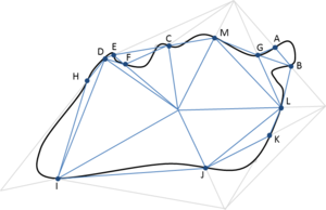
| |
| (e) Second iteration. As there are no nodes to be moved, edges with intersections are split. There is an edge with three intersection points. Point is chosen (arbitrarily) for the splitting. | (f) Final configuration of the mesh. |
The accomplishment of the topology criterion (a) allows the presence of edges intersecting twice the domain in the mesh coming from the tetrahedra pattern. For this reason the moving and splitting process has to be applied the second time to the iso-edges (step 4). The involved iso-edges this second time have at least one of their nodes onto the input boundaries (as they have already been processed the first time).
A 2D example applying two times the process of moving nodes and splitting edges is shown in Table 1.
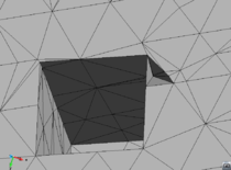
|
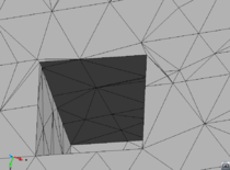
|
| (a) | (b) |
| Figure 53: Example of mesh generated applying (a) or not applying (b) the process of moving nodes and splitting edges the third time. It can be appreciated in Figure (a) that the topology of the mesh near a forced edge does not represent well the topology of the domain. | |
For pathological situations, applying a third time the process of moving nodes and splitting edges is needed (step 5). These pathological situations happen when some of the new edges created in the previous steps has an intersection point relevant for the topology of the mesh. These cases occur near sharp edges, so the iso-edges involved are only the ones connected to a forced node in edge. An example is shown in Figure 53, where the difference between applying or not the moving and splitting process the third time can be appreciated. If there were not forced edges it will not be needed to repeat a third time the moving and splitting operations, because a set of tetrahedra would already represent topologically well each volume of the domain.
One can think about repeating the process of moving nodes and splitting edges as many times as needed until the mesh does not present any intersection point. This is not feasible as it could lead to almost infinite loops (in some configurations with curved input boundaries). Also, each time it is applied, the new elements will have worse quality.
As explained before, the process of moving nodes may create new intersection points. Also the splitting process can create more of them, as it implies the creation of new tetrahedra with the corresponding new edges. The new edges created may have more than two intersections with the input boundaries, but these intersection points are not relevant to preserve the topology of the volumes, so it is not needed to take them into account.
A 2D example of the described surface fitting process is depicted in Table 1. In this example, the process of moving and splitting could be repeated more times, as there are more intersection points (in edge of the mesh shown in (f)). However, the topology of the input boundaries is already well represented, so no more iterations are needed.
5.3.7 Tetrahedra coloring
Once the surface fitting and preserving features operations have been performed, the mesh is in the following situation: it is ensured that the tetrahedra represent the topology of the input boundaries, and all the nodes of the mesh are colored (it is known if they are inside a volume or onto interfaces between volumes). Now the operation of tetrahedra coloring must be done: this is, assign a volume to each one of the tetrahedra. In this work the concept of assigning a color to an entity is used to determine inside which volume the entity is, so color and volume are used indistinctly.
The tetrahedra to be colored can present two basic situations:
- At least one node of the tetrahedra is inside a volume (inner node).
- All the nodes of the tetrahedra are onto interfaces between volumes (surface or line entities). From now on this kind of tetrahedra will be referred as interface tetrahedra.
Tetrahedra presenting the first situation are obvious to be colored. Because of the topological refinement criteria and the surface fitting properties, it is ensured that there is no edge of the the tetrahedra with nodes inside different volumes. This implies the tetrahedra belongs to the same volume of the inner node.
The second situation (interface tetrahedra) is much more complicated to solve. It has to be noted that each node of an interface tetrahedra is interfacing a number of volumes; they are the so called possible volumes of a node. Considering the forced edges lying on an interface between volumes, the concept of possible volumes of a forced edge can be defined analogously as for the nodes.
The possible volumes of each tetrahedron are clearly identified: they are the volumes which are interfaced by all the nodes of the tetrahedron. There are some configurations under which the color of an interface tetrahedron can be determined. This is the case where the tetrahedron has only one possible volume. The rest of interface tetrahedra are considered as undetermined ones; these are the cases that must be solved.
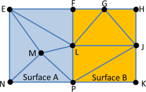
|
| Figure 54: 2D example of a triangle mesh of two surfaces: A (blue) and B (orange). Elements containing node are directly colored as , as is a inner node to A. The other triangles are interface elements. Elements and are undetermined, as they have two possible colors: and (exterior). |
A 2D example of these different types of elements (in terms of coloring process) is shown in Figure 54. Here the mesh for two surfaces ( in blue and in orange) is shown. All elements containing node belong to surface , as is an inner node to . The other elements are interface ones. The possible colors of each one of the interface nodes are listed in Table 2 (note that the outer part of the domain is considered as color zero):
| Node | Possible colors |
| E | , |
| F | , , |
| G | , |
| H | , |
| J | , |
| K | , |
| L | , |
| N | , |
| P | , , |
Considering the interface elements, their possible volumes can be easily gotten analyzing the common possible volumes of each one of their nodes. They are depicted in Table 3.
| Element | Possible colors |
| ELF | |
| FLG | |
| HGJ | , |
| JPK | , |
| JLP |
It can be seen that the elements and are undetermined in this example, as they can belong (topologically) to surface or the outer part of the domain indistinctly.
As each undetermined tetrahedron has more than one possible volume, there are several possible configurations of colors for them. A configuration is understood as the assignment of a color to each one of the undetermined tetrahedra. It has to be noted that the triangles of the skin meshes of each volume are the faces of the tetrahedra shared by tetrahedra of different color, so each configuration of colors lead to a different tetrahedra skin mesh. Taking care about the topology of the input boundaries, the final configuration of colors has to accomplish the following conditions to be considered as valid:
- Between the tetrahedra surrounding one node, it must be at least one tetrahedron for each possible volume of the node. This implies, for example, that the tetrahedra surrounding a node in interface cannot be all of them of the same color.
- Between the tetrahedra surrounding one forced edge, it must be at least one tetrahedron for each possible volumes of the forced edge.
- Considering the input boundaries in the near region from a given node in interface, if the input boundaries are manifold in this near region, the skin of the tetrahedra surrounding the node must be manifold. This condition can only be applied for watertight volumes and implies, for example, that if a node is in a manifold region of the input boundaries, there must be a closed loop of triangles around the node in the skin of volume's tetrahedra.
- The mesh of a volume must present the same topology as the volume. This means, for example, that if the volume has holes, its mesh must have also holes.
The accomplishment of these conditions can reduce to one the possible colors of some tetrahedra. In this cases, these ones would not be undetermined. However, other tetrahedra may remain undetermined.
A good 2D example of undetermined elements considering only two different colors (interior and exterior) is shown in the (f) figure of Table 1 (see page current). The triangles , , , , , and have all their nodes in the boundaries. , and are not undetermined elements, as they can only be colored as inside the surface taking into account the first condition defined above: if they were colored as outside, nodes , and respectively won't have any element inside the surface, and they are nodes interfacing the surface and the outer part. Then, in this example, the elements , , and are the undetermined ones. These elements could be colored as interior or exterior each of them, and both situations may lead to topologically correct meshes. This example shows that the problem of coloring the undetermined tetrahedra has more than one solution, and it is not obvious (actually, in some cases it is impossible) to determine whether a solution is better or worse than another.
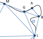
|
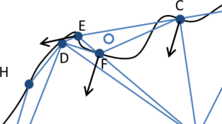
|
| (a) | (b) |
| Figure 55: 2D examples of pathological configurations for element coloring. Both cases are taken from the mesh shown in (f) figure of Table 1. (a) The element is a triangle of the surface, but its center (white dot) is outside it. (b) The element could be colored as inside or outside of the surface; the oriented normal vectors in nodes , and does not point to the center of the element. Black arrows are the oriented normal vectors towards the surface, and the white dot is the center of the triangle. | |
A possible strategy for the tetrahedra coloring should be to assign the tetrahedra the color of their center using the node coloring technique explained in Chapter 4, but this can lead to wrong decisions as there are several pathological configurations where the center of an element of a volume is not inside it. This is the case of triangle in (f) figure of Table 1. A zoom of this triangle is shown in Figure 55(a): is topologically a triangle of the surface , but its center is outside it.
Another possible strategy for undetermined tetrahedra should be take care about the normal vectors of the interface surface entities in the nodes of the tetrahedra. This normal vector can be oriented in the sense that it can be determined which volume it is pointing to (between the volumes interfaced by the surface entity). The notation oriented normal to a volume V is used from now on to indicate the normal vector of a surface entity pointing towards the volume V.
The computation of the normal of a surface of the volume is not obvious taking into account that the contours of the domain can be non-watertight. We are leaving this aspect unsolved by now, and let us suppose the oriented normal vectors can be created. One could think about situations which the oriented normal vectors can determine whether the color of a tetrahedron is one or another depending on where they are pointing to. For example: the cases where the four normal vectors of an interface tetrahedron (one for each node) oriented to a given volume are pointing at the center of the tetrahedron could be considered as determined: the color of the tetrahedron should be the volume one. (In this context, point to the center of a tetrahedron means that the center is in the semi-space defined by the oriented normal vector).
Unfortunately, not all the tetrahedra accomplish with this condition, so there may still be some undetermined tetrahedron. This is the case presented in Figure 55(b): it is a 2D case where it can be seen that the oriented normal vectors to the surface in the nodes of the element are not leaving the center of the element in the same semi-space.
Furthermore, the same topological situations can be represented by different volume boundaries which present a drastically different configuration of normal vectors in the nodes of the elements. This is the case shown in Figure 56, where different interfaces between surface and present the same element with the normal vectors in two of its nodes identical, and the third normal different for each shape of the boundaries. This 2D example demonstrates that the process of tetrahedra coloring cannot be based on the normal vectors of the interface entities in the nodes of the elements. It has to be taken into account that in 3D the possible configurations are much more complicated than in 2D.
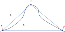
|
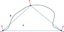
|

|
| (a) | (b) | (c) |
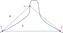
| ||
| (d) | ||
| Figure 56: 2D example. The black curved line represent the interface between surfaces and . (a), (b), (c) and (d) represent different shapes of the interface. In all the cases an undetermined triangle is depicted and the vectors are the normal vectors pointing to surface . As it can be seen, in all the cases the element should be colored as inside surface . The normal vectors in two of the nodes are identical for all the cases, and the third (the upper one) is different in all of them. | ||
The reason why the two strategies defined above fail is they are based on geometrical conditions, and the problem to solve is more topological than geometrical. The color of an undetermined tetrahedron is independent on the percentage of the element inside or outside a volume: it is determined for topological conditions (the ones defined previously). To take care about the topology, a strategy is proposed to color the undetermined tetrahedra starting from the tetrahedra with known color. It is based in the following proposition:
Proposition 1: Considering an undetermined element and an element of color which is neighbor of by face . Being the node of opposite to face , if there is a point inside volume laying on face , and a continuous curve in space from to completely inside element with no intersection with the boundaries of A, then the color of is .
A graphical view of this proposition in a 2D case is shown in Figure 57. In this example the element is undetermined, as all its nodes are on the interface between surface and the outer part of the domain. All the other elements are fully determined (they belong to surface ), as they contain node , which is inner to . Point is inner to , and it lays on the face shared by elements and . As it exists a continuous curve (shown in dotted red line) from to , totally inner to element and with no intersections with the boundaries of , element can be considered inner to surface . It has to be noted that this process imply the coloring process of point , which is done following the algorithm described in Chapter 4.
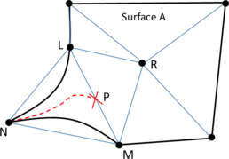
|
| Figure 57: Graphical interpretation of Proposition 1 in a 2D example. The black line represents the contour of surface , and its triangle mesh is represented by blue lines. |
Proposition 1 is used to color the undetermined tetrahedra (the implementation of the algorithm is detailed in Section 6.5). However, it cannot be applied in some cases as the ones where an undetermined tetrahedron has no neighbor by face with a determined color, or the cases where the points in the common face are onto a surface entity (they are not inner to a volume), or the coloring process of these points fails. Another case where the proposition cannot be applied is when the volumes involved are non-watertight. For this reason, it has to be planned that after this coloring process some undetermined tetrahedra can still remain. From now on the methodology to color the remained undetermined tetrahedra is explained.
As it can be seen, the coloring of one tetrahedron can affect the coloring of its neighbors, as the skin of the tetrahedra changes and can affect the manifold condition of each node. However, each tetrahedron affects only to its neighbors, so there can be defined different clusters of undetermined tetrahedra which are independent one from each other; these clusters are made by the undetermined tetrahedra connected at least by one node. As an example, the clusters of undetermined tetrahedra of the mesh in figure (f) of Table 1 are identified in Figure 58. As these clusters are independent one from each other, the methodology presented can be applied on a cluster by cluster manner.
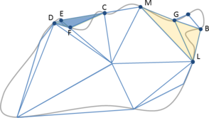
|
| Figure 58: Two clusters of undetermined elements (blue and orange) of the mesh shown in (f) figure of Table 1. |
Considering all the undetermined tetrahedra of a cluster, each of them has its possible colors. All the possible color configurations can be obtained, and each one of these configurations implies a different skin mesh of each volume's tetrahedra. Checking the topological conditions that must be accomplished (detailed previously in this section) for the final mesh, some of the configurations are not valid, and some of them are valid. For the tetrahedra coloring purposes, any one of the valid configurations is set as the solution.
As an example, lets see the case of the orange cluster of undetermined elements shown in Figure 58. It is made of two elements: and . Each of them has two possible colors: inside or outside the surface. All the different configurations are shown in Figure 59. The configuration shown in Figure 59(a) is not valid because the topology of the final mesh is not the same as the one of the surface it is representing (the mesh has two unconnected sets of elements). The configurations of Figure 59(b) and (c) are not valid because they have non-manifold nodes in regions where the contour of the surface is manifold (node in case (b) and node in case (c)). The only valid configuration is the one shown in Figure 59(d).
| ||||||||
| Figure 59: Zoom of the orange cluster of elements in Figure 58. All the possible configurations taking into account the different colors (inside or outside the surface) of elements and .(a) Both elements are outside the surface. (b) is outside and inside. (c) is inside and outside. (d) Both elements are inside. |
5.3.8 Make-up and smoothing
The make-up and smoothing operations are used to improve the quality of the mesh once it has been generated. Make-up operations are the ones changing the topology of the mesh, and smoothing process only implies movement of the nodes, maintaining the original connectivity of the elements.
The acceptable quality of the mesh elements is a relative parameter, as the mesher aims to be applied to different kinds of numerical simulations, and they are applicable in different ranges of qualities for the elements [5]. A clear example of this is the boundary layer meshes, which elements should have an aspect ratio higher than 10000 in some cases; such distorted elements are not valid for standard FEM analysis. However, almost all the methods require non-inverted elements. This means that the Jacobian of the transformation of the element (from the parametric to the 3D space) should be positive. This lead to require, at least, a strictly positive Jacobian in the elements of the final mesh. A graphical interpretation of an inverted element is provided in Section 5.3.3.
In this section there are references to tetrahedra, triangles and edges. Edges are edges of the tetrahedra elements, and triangles are considered as the faces of the tetrahedra interfacing tetrahedra of different color. Thus, each volume tetrahedra mesh is surrounded by a triangle mesh.
Considering the mesh generated may have forced nodes and forced edges, there are some restrictions to be applied to the make-up and smoothing operations:
- Forced isolated nodes (Section 5.3.2) cannot be moved nor deleted.
- Forced nodes in edge which are extreme of a polyline entity (Section 5.3.1) cannot be moved nor deleted.
- Forced nodes in edge can only be moved along the polyline entity they belong to.
- Forced interface nodes can only be moved lying onto the surface entity they belong to.
- If both extreme nodes of a tetrahedron edge are forced nodes in interface and the edge is not a triangle edge, the edge cannot be collapsed.
- If both extreme nodes of a tetrahedron edge are forced nodes in edge and the edge is not a forced edge, the edge cannot be collapsed.
- If a tetrahedron edge has one forced node in edge and one forced node in interface, it cannot be collapsed.
From now on, the operations involving the collapse of an edge, or the movement of a node are only applied to the entities not violating these restrictions. It has to be taken into account that the collapse operation involves the deletion of one of the two nodes involved.
The elements obtained from the tetrahedra pattern defined in Section 3.3.3 have very good quality if the nodes are in the octree positions (see Section 3.3.2), so the make-up and smoothing operations are only needed for the tetrahedra containing a forced node, the ones coming from interface cells and the ones resulting from surface fitting or preserving features operations.
The parameters and (Section 5.3.5) try to guarantee a minimum quality in the tetrahedra resulting from the preserving features process, and tries to do the same for surface fitting operations. However, some configurations of the mesh and the input boundaries may lead to low quality elements. This situation often causes the presence of small edges in the mesh. An example of these small edges is shown in Figure 60(a). To improve the quality of the elements surrounding these small edges, an edge collapsing step is performed (make-up operation). Taking into account that the octree cell containing each node gives an idea of the mesh size required for the mesh in that region (because of the user desired sizes or as a result of a topological refinement process), the edges smaller than a given portion of the size of the cell they are inside are collapsed. An edge is collapsed if it does not violate the restrictions defined at the beginning of this section and
|
|
(5.5) |
where is the size of the smaller octree cell between the ones where the extreme nodes of the edge are inside, the length of the edge and is a real value greater than zero. Its value is discussed in Section 6.7.

|
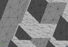
|
| (a) | (b) |
| Figure 60: Example of a mesh (a) before and (b) after the make-up and smoothing process. | |
The smoothing operation applied consists in a Laplacian-like smoothing that displaces a node into a position such that its surrounding elements improve their quality. The smoothing process is applied on a node by node basis, and follows these steps:
- Compute the quality of all the tetrahedra surrounding the node, and identify the worst of them ().
- Move the node to a candidate position.
- Compute the quality of the tetrahedra surrounding the node in the new configuration and identify the worst of them ().
- If is better than , the node is left in the candidate position, otherwise, the node is returned to its original one.
This process implies the definition of a quality measure of the elements, as well as a procedure to obtain the candidate position. As a quality measure, the minimum dihedral angle of the tetrahedra has been chosen, considering that a tetrahedra is worse than another one if it has a lower minimum dihedral angle. The election of the candidate position is explained later on.
It has to be noted that the mesh can have three kinds of elements: tetrahedra, triangles and linear elements (corresponding to the forced edges). All the nodes have tetrahedra around them, but only some of them have triangle or linear (1D) elements. Taking into account the restrictions defined in the beginning of this section, the degrees of freedom for moving a node are restricted by its nature: if it is a forced node in edge, it can only move along the polyline entity corresponding to the forced edge, and if it is a forced interface node it must lay on the surface entity it belongs to. This aspect governs the candidate position for each node:
- If the node is a forced node in edge, the mean position of the opposite nodes of the forced edges it belongs to is calculated. Considering the polyline entity those forced edges come from, the candidate position is the closest point to laying on the polyline entity.
- If the node is a forced interface node (it has triangles around it), all the nodes of the triangles around it (except the node itself) are considered. Their mean position is calculated, and the candidate position is the closest point to laying on the surface entity the triangles belong to.
- If the node has no triangles nor forced edges, the candidate position is the mean position of the nodes of the surrounding tetrahedra of the node (except the node itself).
As the movement of a node affects the quality of all its surrounding elements, the smoothing operation is thought as an iterative process where several loops over all the nodes are performed in order to improve the quality of the mesh.
Apart from edge collapsing and nodes smoothing, the edge flipping operation (a make-up operation) is performed in the mesh [55]. The cases 2 to 3, 3 to 2, 4 to 4 and 5 to 6 are implemented. These operations imply the removal of a face (the first case) creating an edge, or the removal of an edge (the other cases) creating some extra faces. Apart from the pathological configurations described in [55] which determine the situations where the edge flipping cannot be made, some topological configurations must be considered in order not to invalidate the topology of the mesh generated. In particular, the following restrictions are considered:
- If an edge is a forced edge or the edge of a triangle, it cannot be deleted.
- If a tetrahedra face is a triangle of the mesh, it cannot be deleted.
The collapse, edge flipping and smoothing operations are applied in a sequential iterative manner to account for the updated configurations of the mesh each time. A maximum of four iterations is set in the present work. The result of applying them to the mesh shown in Figure 60(a) is depicted in Figure 60(b). In Chapter 7 several examples are shown indicating the mesh quality before and after the make-up and smoothing operations.
5.3.9 Mesh quality
This section focuses in the analysis of the quality of the final mesh generated by the new mesher.
For the embedded mesher, the quality of the mesh is totally guaranteed, as all the tetrahedra come directly from the predefined patterns. However, for the body-fitted mesher, it has to be considered that a body-fitted mesh is forced to respect the boundaries of the domain. If a part of the domain is bounded forming a very small dihedral angle, the tetrahedra representing it will have the same dihedral angle. This limits the scope of minimum quality guarantee to the inner parts of the domain, or the boundaries which are relatively smooth.
The tetrahedra of the inner parts of the domain come directly from the predefined patterns, so they have a very good quality. Their minimum dihedral angle is degrees (Section 3.3.3). For the tetrahedra near the boundaries there are several aspects that make impossible to ensure a minimum quality for the elements in the final mesh:
- Forced nodes. As the forced nodes are not placed in the octree positions, the tetrahedra pattern generated may yield tetrahedra that are distorted with respect to the ones coming from regular octree nodes. The tetrahedra distortion refinement criterion (RC 7) avoids inverted tetrahedra, which ensures a minimum dihedral angle equal to zero. A solution could be to set a higher minimum dihedral angle, thus ensuring a better quality for the elements. However, considering that the boundaries of the domain may have small dihedral angles, this could lead to infinite refinement in certain regions, because it may be impossible to represent a given shape from a tetrahedron coming from an octree cell.
- Preserving forced edges operations. These operations involve displacement of nodes and split of tetrahedra edges and faces. Parameters and govern the behavior of these operations. Depending on the position of the intersection point of the forced edge and the given tetrahedron face, these parameters establish whether a node must be displaced or a splitting operation must be performed. Theoretically, the tuning of these parameters could bound the quality of the final configuration of tetrahedra after these operations, if the minimum element quality of the initial configuration is known. This is not the case, because of the presence of forced nodes (as explained in the previous paragraph), so a minimum element quality cannot be ensured after the process of preserving the forced edges.
- Surface fitting process. The isostuffing method [37] ensures a minimum element quality by tuning two parameters that govern the decision of moving a node or splitting an edge in the surface fitting process. This is possible because the method does not preserve the geometrical features. The mesh where these operations are applied comes directly from a predefined tetrahedra pattern, which quality is known a priori. In our case, the quality of the mesh before the surface fitting process is not bounded, as explained in the previous two points. Hence, the tuning of the parameter tries to get well shaped tetrahedra, but cannot guarantee any minimum quality for the final mesh.
For all these aspects, although the make-up and smoothing operations described in Section 5.3.8 reach an acceptable quality for the meshes generated, a given minimum element quality cannot be guaranteed theoretically.
5.3.10 Extension for surface meshing
As explained in Section 1.2.4, a secondary objective of the present work is to be able to apply the octree mesher to the meshing of surfaces not belonging to any volume. In this section the concept of inner surface is used to refer a surface entity not belonging topologically to the boundaries of a volume. It can be inside or outside a volume. From the mesher point of view this difference takes no sense as the outer part of the model is considered as volume zero.
Taking into account the new mesher can provide with the surface mesh corresponding to the boundaries of a volume, it could seem that it can be applied directly to an inner surface. Actually, after the surface fitting process there are tetrahedra at both sides of the inner surfaces that conform to them. However, the faces of the tetrahedra which form the triangle mesh of the inner surface cannot be detected in the same way as the surface entities boundary of a volume (regural surface entities).
Extracting the surface mesh of a regular surface entity is automatic after the process of tetrahedra coloring (described in Section 5.3.7): the triangles of the surface entities are the faces of the tetrahedra interfacing two tetrahedra of different color. In the case of inner surfaces, tetrahedra at both sides of the triangles have the same color, so the same strategy cannot be applied. Some modifications have to be performed in order to detect the triangle mesh of an inner surface.
At the time of extracting the surface meshes of the inner surfaces all the tetrahedra have been generated, the processes for preserving geometrical features and surface fitting have been carried out, and the tetrahedra have been colored. At this point, there are already tetrahedra faces corresponding to the triangles of the inner surface mesh, but they have to be detected. This situation is illustrated in Figure 61(a) using a 2D example (an inner line and the surrounding triangles is used instead of an inner surface and the surrounding tetrahedra).

|

|
| (a) | (b) |

|

|
| (c) | (d) |
| Figure 61: 2D example of the steps for detecting the line elements of an inner line. (a) Initial configuration: elements at both sizes of the inner line. Thick black line is the inner line and the mesh is in blue. Black dots are forced nodes in interface or in edge. (b) All the candidate 1D linear elements in dotted black lines. (c) Candidate 1D linear elements (in black) accomplishing the topological properties set to definitive. (d) Final mesh (in black) for the inner line once the remaining invalid candidate linear elements have been discarded by Proposition 2. | |
A first consideration must be done: all the triangles in the mesh of a surface entity have their nodes laying on it. This means that the nodes of those triangles are forced nodes in interface or in edge. The tetrahedra faces with this characteristics (all their nodes being forced nodes in interface or in edge) are called candidate triangles. In Figure 61(b) the candidate linear elements (in 2D there are candidate 1D linear elements instead of candidate triangles) of the configuration shown in Figure 61(a) are depicted in dotted lines.
Considering all the candidate triangles of an inner surface, some topological properties analogous to the ones made in the tetrahedra coloring strategy can be done. If a node is inside a surface entity, the surface mesh around it must be manifold (let us call it a manifold node). This implies that there should be a closed loop of triangles surrounding it in the mesh of the surface entity. If there are a closed loop of candidate triangles around a manifold node, and they are the only candidate triangles containing the node, they can be set as valid (triangles belonging to the inner surface final mesh). Also the requirement for every forced node in interface or in edge to belong at least to one triangle of the final mesh can be used: if one of these nodes belongs to one candidate triangle only, this one must be valid. For the case shown in Figure 61(a), the candidate elements set as valid considering these topological properties are depicted in Figure 61(c).
However, this topological properties may not solve the problem of detecting all the triangles of an inner surface mesh, as there are nodes which are not needed to be manifold (the ones in edges), and there may be triangle configurations around manifold nodes which are not manifold. This leads to the need for another strategy to detect the right triangles among all the candidate ones. The strategy proposed is based on disregarding the wrong candidate triangles, rather than detecting the right ones, using Proposition 2. It is based on Proposition 1 (defined in section 5.3.7 for tetrahedra coloring), but with slight modifications:
Proposition 2: Consider a candidate triangle of an inner surface and the two tetrahedra around it and . Being and the nodes of and not belonging to , if there is a point inside triangle and a continuous curve in space from to passing through completely inside the union of and with no intersection with , the candidate triangle is invalid.
A graphical view of this proposition(using a 2D case) is shown in Figure 62.
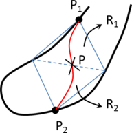
|
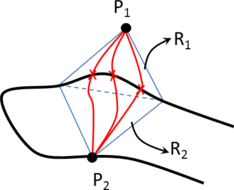
|
| (a) | (b) |
| Figure 62: Graphical interpretation of Proposition 2 in a 2D example. Black line represents the inner line (). Triangle mesh is represented by blue lines and the candidate linear element to be checked () is the dotted line. (a) The candidate linear element is invalid, because there is a curve (in red) not intersecting the inner line. (b) The candidate 1D linear element cannot be set as invalid because all the possible curves intersect the inner line. | |
In Figure 62(a) the candidate 1D linear element is set as invalid because there is a curve (drawn in red) accomplishing Proposition 2. Figure 62(b) shows that there could not be any curve accomplishing the proposition, so the candidate linear element cannot be set as invalid.
Once all the invalid candidate triangles are disregarded using Proposition 2, the rest of the candidate triangles are the ones corresponding to the final mesh of the inner surface (Figure 10(d)).
Note that this proposition can set as invalid some correct triangle in some cases, specially when the the surface entities are curved. Some improvements should be applied to the algorithm to be more robust in some pathological configurations.
The implementation of the algorithm defined for extracting the mesh of an inner surface is detailed in Section 6.5.4.
6 Implementation aspects
This chapter details all the implementation aspects relevant for the meshing algorithm described in the previous chapters. The specific implementation of the ray casting technique used for the nodes coloring is explained in Section 4.3, as it can be considered as an independent process.
It is important to note that implementation matters do not affect the result of an algorithm, but they affect its performance and efficiency. In this sense, the implementation of a meshing algorithm is crucial if it has to be applied to industrial problems with complex geometries, or to generate really large meshes. A bad implementation can lead to unaffordable problems in terms of memory and computational time.
The algorithm has been implemented as a static library. Although the implementation of the mesher is done taking into account the GiD pre and post-processing system [56,57,58] for getting the input data and the visualization of the meshes, its connection to GiD has been done as an external library, by a general interface specially designed to make it accessible for other programs. It is really important to provide access to the mesher as a library, as some numerical simulations require interaction with the mesher during the simulation itself (i.e. for optimization loops or in remeshing processes).
6.1 General aspects
The implementation of the new algorithm has been carried out paying special attention to saving as much memory as possible, and trying to improve its performance taking into account shared memory parallel processing (Section 6.6).
One important characteristic common to many meshing algorithms is that they need an extra memory to generate the mesh compared to the memory needed to store the mesh once it has been generated. This leads to the need of memory saving strategies in the implementation of the mesher:
- The main part of operations involving octree cells are applied only to inner and interface cells (not to outer ones), so they are the ones from which the tetrahedra are generated. These operations include cells refinement and creation of octree nodes. It has to be considered that in the first stages of the meshing algorithm it is not obvious to know if a cell is outer or not, as the coloring operations are not done yet. For this reason, in these stages a simple check is made in order to detect some of the outer cells in an easy way: if the cell is outside the bounding box of the model, it is taken as an outer cell. Checking whether a cell is inside or outside a bounding box is a really inexpensive process.
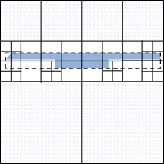
|
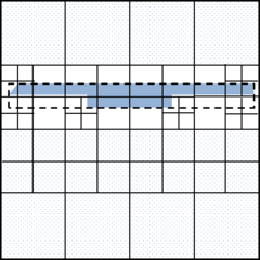
|
| (a) | (b) |
| Figure 63: 2D example of a thin model (the solid surface) with its bounding box (dotted line) and the quadtree (black lines). Cells out of the bounding box are marked with points. (a) Quadtree refined considering only the cells colliding the model bounding box. It can be appreciated that the quadtree is not balanced out of it. (b) Quadree refined considering all its cells. | |
Depending on the aspect ratio of the bounding box of the model, this strategy can save a lot of memory. This is the case of very thin models in some direction (like the 2D example depicted in Figure 63) where, actually, the main part of the octree root is out of the bounding box of the model. Not considering the refinement criteria of the octree out of the model bounding box (like, for instance, the balance criterion) can reduce drastically the number of cells of it, as it can be seen in Figure 63. It can be appreciated that the quadtree refined considering all the cells (b) has much more cells than considering only the cells colliding the model bounding box (a).
- Tetrahedra from the inner part of the volumes are generated at the very last step of the algorithm. Tetrahedra from the inner leaves have really good quality, they are not affected by the operations involved in the body-fitting process (preserve geometric features and surface fitting) and their color is totally determined (all its nodes have the same color). For this reason, these tetrahedra can be generated in the last step of the algorithm without affecting the resulting mesh. This part is implemented as follows:
- Once the octree is refined following all the refinement criteria, the interface cells and their neighbors (one level of neighborhood) are considered. Then, their tetrahedra are generated.
- The following operations are performed on these tetrahedra: preserve geometrical features, surface fitting process, tetrahedra coloring and make-up and smoothing operations. These operations require typically an extra topological information of the mesh (like the neighbor elements of a node). Once these processes are finished, this extra information is deleted in order to save memory.
- Then, as a last step, the tetrahedra generated from the inner cells are created. In this step no additional information than the mesh itself must be stored.
The flowchart of the body-fitted algorithm illustrating this process can be seen in Figure 69.
Considering the input data, the meshing algorithm is designed in a way that the input boundaries can be mesh or geometrical entities. The only operations required for them to be used in the algorithm are:
- Get the bounding box of the entity.
- Compute the intersection between an edge and the entity.
- Get the closest point of the entity to a given position of the space.
The algorithm has been implemented considering only mesh entities for the definition of the input boundaries. This simplify much the geometrical operations defined above.
6.2 Octree implementation
The octree is the key structure of the presented algorithm. As mentioned in previous sections, it is not only used for generating the tetrahedra, but also for searching purposes. Actually, octrees were created originally for this topic, so it is natural to take advantage from on its characteristics in this field.
The main operation the octree is designed for is to find the leaf containing a coordinate in space. For this purpose, beginning from the octree root, the given coordinate is analyzed to evaluate which of its children contains it (considering the uniform subdivision of a cell, determining in which octant of a cell the coordinate is represents an inexpensive process). If the child is not an octree leaf, the process is repeated (with itself instead of the octree root) until an octree leaf is reached. This process can be seen as going downstream by the octree structure, and often implies the use of recursive functions (the same function applied to a cell is applied to its child). The use of recursive functions is not desirable because it decreases the performance of the algorithm due to the function call overhead.
In order to achieve a good performance, a very efficient implementation of the octree has been carried out based on [43] work. This octree has the peculiarity that works in the normalized unitary space xx. This is required because it uses the binary representation of all the coordinates involved in the process casted to integer: the so called key of the coordinate.
From a given coordinate in the normalized space, the following steps are performed in order to find the octree leaf containing it:
- Get the key of the coordinate: it is the representation of the coordinates in binary form (i.e. for coordinate the binary representation will be ).
- For each level of the octree (beginning from the octree root), the ith bit of the key representation is used for selecting the left or right child for each coordinate ( for left and for right child). In each level, having the combination of three coordinates bits provides the correct decision of the child.
The identification of a cell is done by its lower coordinate using the corresponding key; it receives the name of the location code of the cell. A graphical view of a 1D binary tree is depicted in Figure 64. Each one of the nodes represents a cell, and its key is depicted. For the leaves (the cells in the last level) the coordinate in the unitary space is also shown (framed). Checking the keys of the different cells it can be appreciated that traveling downstream the tree is really easy looking at the bit corresponding to the level of the cell: if the bit is take the left branch, and if it is , take the right one.
A detailed description of the algorithm can be found in [43] including its 2D implementation, as well as how other basic operations in octree are done (like traversing from a cell to another).
![Binary tree representation of a 1D spatial partitioning over [0,1] indicating the cell's location code (its key) and its corresponding coordinate (inside frames) of the leaves cells.](/wd/images/thumb/5/52/Draft_Samper_249832658-monograph-octree_tree.png/420px-Draft_Samper_249832658-monograph-octree_tree.png)
|
| Figure 64: Binary tree representation of a 1D spatial partitioning over indicating the cell's location code (its key) and its corresponding coordinate (inside frames) of the leaves cells. |
This implementation of the octree forces to work in a normalized space (between and in each dimension). As it will be seen in Section 6.5, some geometrical transformations are performed on the input boundaries and the sizes information from the input data in order to fulfill this requirement.
One important advantage of using the keys instead of the coordinates, is that they are integer values while the coordinates are real ones. Some geometrical operations profit from this, like the detection of nodes aligned with the Cartesian directions. If two nodes have the same coordinate (in some direction), its real value can be slightly different because of the storing procedures of the computer. However, their key, as an integer, is the exact same number. This aspect is used in the ray casting implementation and other parts of the algorithm.
The main characteristics of the implemented octree are:
- The octree is represented in a hierarchical tree structure composed of a root cell, intermediate cells and leaf cells.
- Each cell stores pointers to each child cells, but not to its father cell. This reduces the memory used by the octree.
- The operation of traveling downstream of the octree is not recursive. As it have been seen, knowing the key of the coordinate to be analyzed is enough to take the corresponding branching decisions in a global way.
- The maximum number of octree levels is 30. This is the direct result of storing the key as a 32 bit integer. Due to some implementation issues the minimum level must be 2, so in practice the octree can have 30 levels. This implies that the smallest octree cell can be of the bounding box.
The memory usage can be improved by keeping only the leaves and making a hash function to search leaves as the work of [59]. Also the performance of the octree can be improved by precomputing the bit shifting in each level and the traversing algorithm can be improved by creating a parents trace from root to leaves in time of traversing as proposed in [60]. However, the current implementation is good enough for the meshing algorithm developed in this work, as it is not a bottle-neck in terms of speed nor memory.
In the new meshing algorithm, the main role of the octree is to create the tetrahedra from given patterns. For this purpose each octree leaf has its octree nodes stored. Furthermore, the octree is also used for searching purposes.
Specifically, the octree is used to find in an efficient way the input surface entities near a given node, or near an edge of the tetrahedra mesh. For this purpose, the input surface entities must be stored somehow in the octree. A surface entity can collide one or more leaves. The strategy followed in this work is to store a pointer of each surface entity inside each leaf colliding with it. This option gives a very good performance in the octree operations. The memory consumed for this purpose depends on the ratio between the size of the surface entities defining the domain and the octree leaves sizes. In the examples studied this memory is not relevant, considering the whole process.
6.3 Generalized mesh size points
The generalized mesh size points are a collection of points placed on each mesh size entity in such a way that, being its desired mesh size, there is no point inside the entity further than from a generalized mesh size point (see page current). The idea is to replace the mesh size entities by their generalized mesh size points in order to simplify some of the algorithms involved in the mesher, such as the size refinement criteria.
There are infinite configurations of generalized mesh size points of an entity accomplishing the condition described above. For improving the performance of the global algorithm it is necessary to find a simple way (computationally inexpensive) of obtaining a configuration of them trying to minimize its number.
The distribution of sizes of the leaves of the octree is not continuous (a leaf can have the same, the double or half of the size of its neighbor). However, the desired mesh sizes imposed by the mesh size entities can take any real positive value. To take into account this, the parameter is used to scale the desired size of a mesh size entity when creating its generalized mesh size points. The scaled size of a mesh size entity is defined as:
|
|
(6.1) |
where is the desired mesh size of the mesh size entity and is a real value greater than one. The value used in the presented implementation is detailed in Section 6.7.
There are four kinds of mesh size entities: point, line, surface and volume entities. The presented implementation has been done considering the following mesh element types as mesh size entities: node, linear, triangle and tetrahedron. To simplify the notation, the concepts of mesh size node, mesh size edge, mesh size triangle and mesh size tetrahedron is used to refer to the corresponding entities.
All the generalized mesh size points created from a mesh size entity have a desired mesh size . As can be shared by other higher level mesh size entities (for example, an edge can be shared by some triangles and tetrahedra), takes the lower value between the desired mesh size of the mesh size entities belongs to and the one from itself.
Hereafter, the methodology used for the creation of the generalized mesh size points from each type of entity is presented:
- Creation from a mesh size node. This is the simplest case. From a mesh size node a generalized mesh size point is created in its position with a desired mesh size .
- Creation from a mesh size edge. The extreme nodes of a mesh size edge are considered as mesh size nodes (with a desired mesh size ).
If the length of the mesh size edge is higher than , the edge is subdivided uniformly in divisions, with defined as:
|
|
(6.2) |
where represents the truncated value to the closest integer.
From each position inner to the edge resulting from the edge subdivision a generalized mesh size point is created with a desired mesh size .
- Creation from a mesh size triangle. The three edges of the triangle are considered as mesh size edges (with a desired mesh size ).
Generalized mesh size points from the inner part of the triangle are created only if the three heights of the triangle are higher than . In this case, an auxiliary triangle is created from the mesh size triangle . is similar to (their sides are parallel), it is smaller than and the distance between their corresponding sides is equal to (see Figure 65).
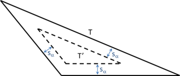
|
| Figure 65: Auxiliar triangle (dotted line) of mesh size triangle (solid line) used for the generation of its inner generalized mesh size points. |
The edges of are then considered. If they all have a length lower than , a generalized mesh size point is created in the center of . Otherwise this strategy is followed:
- If the length of an edge is higher than , it is considered as a mesh size edge (with a desired mesh size ).
- If the length of an edge is lower than , a generalized mesh size point is created in the center of the edge.
- Then the process of creating the auxiliary triangle is repeated from recursively.
- Creation from a mesh size tetrahedron. The four faces of the tetrahedron are considered as mesh size triangles (with a desired mesh size ).
If the four heights of the tetrahedron are higher than , an analogous procedure as for the triangle is carried out (in this case creating an auxiliary tetrahedron) in order to create the inner generalized mesh size points. This process can create extra mesh size triangles, edges and nodes.
6.4 Sizes transition function
This section focuses on the definition of the function, used in the sizes transition criterion. This function provides the upper limit for the mesh size in each position of the domain.
The definition of leans on two main inputs, both from the input data (see section 3.1):
- The mesh size entities. These entities indicate the desired mesh size for the simulation in given regions of the domain.
- The size transition factor (from now on ). is a positive value between zero and one, and controls if the size variation between regions of the domain of different mesh size is smoother or sharper.
From a given position in space , and a desired mesh size defined on it, two functions can be defined ( and ) in order to bound between an upper and lower limit the mesh size in a specific position of space : the size transition functions. Different functions can be used for this purpose in order to fulfill the simulation requirements (in terms of element size distribution). In the present work the following linear functions have been chosen:
|
|
(6.3) |
|
|
(6.4) |
where is the distance between and and takes the following expression:
|
|
(6.5) |
is defined in Section 5.2.2. is the maximum value between the minimum desired size coming from the mesh size entities and the size of the smallest leaf in the octree (so the evaluation of this function depends on the configuration of the octree). is a weight parameter (Equation 6.9) and its interpretation is given hereafter.
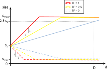
|
| Figure 66: Graph of the size transition functions 6.3 (solid line) and 6.4 (dotted line) with different parameters of . The functions are plotted as a function of : the distance between and . |
A graph of the size transition functions with different values for the parameter is depicted in Figure 66. As it can be seen, for equal to one, is a straight line with a slope equal to one. This corresponds to the maximum variation of mesh size allowed in the octree, which is given by the constrained two to one condition.
The parameter should be tuned in order to set the lower slope of the function (when is equal to ). In order to do so, the following aspects must be considered:
- The distance between two points of the domain is always lower than the diagonal of its bounding box .
- The minimum size transition should allow, at least, to double the mesh size between the furthest points of the domain. This means the sizes of these points differs by a factor equal or higher than two. A factor lower than this could lead to uniform size meshes (without size transition).
These parameters are applied to Equation 6.3 in order to get the expression of . Taking into account above conditions this expression can be written now as:
|
|
(6.6) |
Replacing using Equation 6.5, and considering we are in the case of we get:
|
|
(6.7) |
The expression of can be found from Equation 6.7 as:
|
|
(6.8) |
A factor has been chosen in this work. It can be appreciated in Figure 66 (the function corresponding to ) that the mesh size at a distance is times the one at the origin. This leads to the final expression of as:
|
|
(6.9) |
The selection of these functions has been done mainly for its simplicity. One could think about more sophisticated ones, but it has to be considered that these functions are used for octree refinement purposes. Once an octree cell is refined, its child cells have half of its size. This limits the control of the local mesh size variation and governs the sizes transitions at a more global scale of the domain.
Considering the generalized mesh size points from all the mesh size entities, functions and can be defined from Equations 6.3 and 6.4 when is the position of the generalized mesh size point , and its desired mesh size. Being the number of mesh size points, function is defined as:
|
|
(6.10) |
Analogously, function gives a minimum value for the mesh size in all the points of the domain:
|
|
(6.11) |
The concept of generalized mesh size points has been introduced in Section 5.2.2. As explained before, the presented algorithm works with them instead of the mesh size entities. For this reason, only for notation purposes, from now on mesh size points will be used to refer all the generalized mesh size points.
One option for providing an envelope for the upper limit in the element size covering all the domain could be to use directly the equation 6.10 as . This lead to a mesh size distribution governed by the lower mesh sizes. A graphical 1D example of the function following this approach is shown in Figure 67. Dotted lines are the of each mesh size point, and is the red solid polygonal line (the envelope of ). It can be seen that the mesh size in the extremes of the line () is lower than the desired one () because there is some mesh size point with lower size () assigned near them.
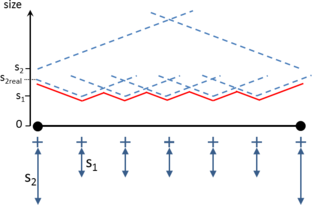
|
| Figure 67: Graphical view of the function for a 1D example (red line). Black horizontal line represents the domain (a line entity) to be meshed with a size equal to . The crosses are the generalized mesh size points. Extreme points of the line have a mesh desired size equal to , higher than . Dotted lines represent the function of each generalized mesh size point. |
In general, it is common to let the small mesh size regions dominate the mesh size distribution all over the domain. However, for many numerical simulations, the mesh size on the contours of a geometrical entity has a special interest. A strategy has been followed in order to try to preserve the mesh sizes on this areas (the contours of the entities). It consists in applying a correction to the desired size assigned to the mesh size points before evaluating Equation 6.10. This correction is done in the following way:
- Classify the mesh size points following the nature of the mesh size entity they come from: point, line, surface or volume entity. This yields four collections of mesh size points (one for each entity type).
- For each group of mesh size points from the lower to the higher level (from points to volumes), execute the following actions:
- Sort the mesh size points of the group according to its desired size (from smaller to larger size).
- For each mesh size point (from small to large size):
- Evaluate functions and of in the positions of the all the other mesh size points. This gives an upper () and lower () size limit for each mesh size point of the model.
- For each mesh size point , check whether its size () is inside the range defined by the limits and .
- If is higher than , then the size of is set to .
- If is lower than , then the size of is set to .
The graphical view of for the 1D example shown in Figure 67 after the correction of sizes for the mesh size points is shown in Figure 68. It can be appreciated that the desired mesh size in the contours of the line entity to be meshed (its extreme points) is not modified (), but some of the inner mesh size points of the line (the closer to the extremes) have a maximum size higher than the one desired ().
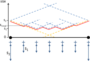
|
| Figure 68: Graphical view of function for the 1D example of in Figure 67, after applying the size correction in the mesh size points. Dotted yellow lines represent the function of the mesh size points corresponding to the extremes of the lines. functions for inner mesh size points are not plotted to make clear the visualization (they are not relevant for the example). |
It has to be considered that the evaluation of and at a given mesh size point only has to be effectively done in the mesh size points around it, as both functions are truncated by and . These values define a radius of influence for each function.
The way this algorithm is implemented takes advantage from the octree structure itself: instead of evaluating the functions from a given mesh size point in all the others, the upper and lower limits provided by the functions are stored in the octree cells surrounding of it (near the radius of influence). Then, to check the size limits of a mesh size point, the values of the octree cell containing it are considered.
6.5 Body-fitted mesher
The main steps of the meshing algorithm for body-fitted meshes are explained in Section 5.3. This section is focused in its implementation aspects. The implementation of the embedded mesher is not detailed because it basically involve the algorithm detailed in Section 5.2 with no more particularities.
A general flowchart of the meshing algorithm implementation is depicted in Figure 69. Its processes involved are listed hereafter (the ones requiring a more detailed explanation are detailed in further sections):
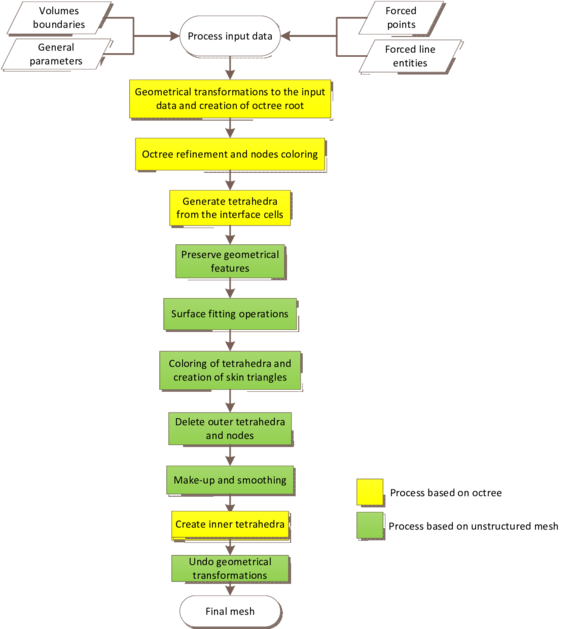
|
| Figure 69: Flowchart of the body-fitted meshing algorithm implementation. |
- Process input data. This step basically consists in getting all the information from the input data: input boundaries, forced entities (points and lines) and general parameters. In this step some new forced entities can be generated in case the input data define some tolerance to detect automatically ridges or corners.
- Geometrical transformations to the input data and creation of octree root. Before the creation of the octree root, some geometrical transformations are applied to the input data (the input boundaries and some of the input parameters) in order to fit it to the implemented octree characteristics, and to improve efficiency in the algorithm. These geometrical transformations are detailed in Section 6.5.1.
- Octree refinement and nodes coloring. This process receives the octree root with all the input data already processed, and ends up with the octree in its final configuration: its leaves will not be further subdivided. The implementation of the octree refinement operations is complex, as it require an iterative process. It is detailed in Section 6.5.2. The coloring of the nodes is done inside this process, so after the octree refinement all the nodes are colored.
- Generate tetrahedra from the interface cells. At this point only the tetrahedra from the interface leaf cells and their first level neighbor leaves are generated following the given patterns (defined in Section 3.3.3). The tetrahedra from the inner part of the volumes have all their nodes in the octree positions (they have no forced nodes), so they have good quality (no further smoothing is needed). Furthermore they are not involved in the surface fitting or the preserving features processes, so there is no need to edit them. The possibility not to generate the inner tetrahedra allows an important memory saving, taking into account that in most models the number of tetrahedra of the inner parts of the volume is much larger than the number of tetrahedra intersecting the volume contours.
This memory saving allows to store extra information in the nodes and tetrahedra (only the ones coming from interface cells) in order to improve the performance of the algorithms. This extra information is mainly related to the neighborhood of nodes and elements.
- Preserve geometrical features. This step involves the operations described in Section 5.3.5, and ends up with all the forced edges and forced nodes belonging to the some tetrahedron of the mesh.
- Apply surface fitting operations. This step involves the operations described in Section 5.3.6.
- Coloring of tetrahedra and create skin of triangles. Tetrahedra are colored (the volume they belong to is determined) following the implementation described in Section 6.5.3. Then, the skin of triangles of each volume of the domain is built with the tetrahedra faces interfacing tetrahedra of different colors.
- Delete outer tetrahedra and nodes. At this point the nodes and tetrahedra owning to the outer part of the domain (color equal to zero) can be deleted.
- Make-up and smoothing. As part of the tetrahedra coming from the inner leaf cells are not generated yet, in the make-up process the nodes belonging to one of these leaf cells must be preserved: they cannot be deleted in the edge collapsing process. As the more distorted elements come from the interface leaf cells, this limitation in the make-up process does not affect the final mesh quality improvement.
- Create inner tetrahedra. In this step the tetrahedra from the inner cells are generated following the given patterns (defined in Section 3.3.3). It has to be considered that these tetrahedra are always determined in terms of color, as all their nodes belong to the same volume.
- Undo geometrical transformations. The inverse of the geometrical transformations applied to the geometrical input data must be applied to the final mesh generated, in order to fit it in the original position of the domain.
6.5.1 Geometrical transformations to the input data
As explained in section 6.2, the octree used is a unitary octree: the octree root goes from the values to for the coordinate in each dimension. This enforces all the geometrical input data (input boundaries, forced entities and mesh size entities) to be transformed in order to avoid any coordinate outside the range . Because of the octree implementation chosen and efficiency matters, before the octree root creation three main geometrical transformations are applied to the geometrical input data:
- Rotation. As explained in Section 3.3, the octree structure chosen for the mesher is isotropic. Considering a domain and its possible solid rigid motion, the way it fits inside the octree is different in the sense that different configurations of cells are intersected by the model. In general, when working with octrees, the more the model shape is aligned to the Cartesian axes the more efficient is the octree in terms of memory and performance. For this reason, the geometrical input data is rotated aligning the main inertia axes of the external skin of the model with the Cartesian axes. It is important to note that the meshing algorithm is valid without rotating the model (this is done for efficiency purposes only).
- Translation. Once the geometrical input data is rotated, a translation is applied to it in order to place the center of in the position which is the center of the octree root.
- Scale. As explained in Section 5.2.3, the octree root is created from and . Considering the octree root must have a unit length, the gometrical input data is scaled to accomplish this condition. All the mesh sizes information in the input data (the general mesh size, or the size assigned to mesh size entities) are also scaled with the same factor.
A graphical 2D example of these three transformations (with a quadtree instead of an octree) is shown in Figure 70.
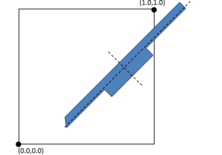
|
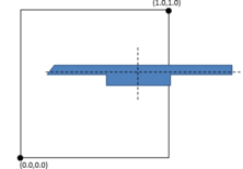
|
| (a) | (b) |
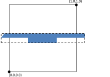
|
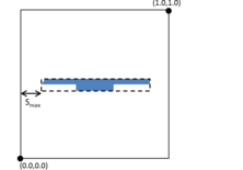
|
| (c) | (d) |
| Figure 70: Geometrical transformations applied to a 2D model before quadtree root creation. Solid surface is the model and the black line the quadtree root. (a) Original configuration of the model and the quadtree root (inertia axes drawn with dotted lines). (b) Model rotated aligning its main inertia axes with the Cartesian ones. (c) Model translated to the center of the quadtree root (bounding box of the model with dotted line). (d) Model scaled leaving an offset of between its bounding box and the quadtree root. | |
A secondary advantage of applying these transformations to the model before the meshing process is that the final mesh is more invariant with solid rigid movements of the input data. This is not a crucial aspect, but it is always desirable that the mesh for a given domain remains topologically identical if the domain is transformed following a rigid solid movement.
In cases where the desired mesh size is uniform in all the domain, an extra transformation can be applied to the octree root after the previous ones. It consists in increasing the size of the octree root until it fits with a power of two of the desired uniform size. Doing so, it is guaranteed that the final mesh will have elements of a size very close to the desired one. Furthermore, there is more control on the number of elements in the final mesh. If this transformation is not done, assigning slightly different sizes to the same model would yield the same mesh.
As an example, generating the mesh of the same model with different uniform sizes (from large to small size), the generated mesh would be identical until the desired size is small enough to force an octree refinement. In this case, the number of elements in the final mesh will be approximately eight times the one of the previous mesh, as refining an octree cell creates eight cells more.
6.5.2 Octree refinement
As pointed out in Section 5.3, the refinement of the octree is an iterative process, because the subdivision of an octree cell may lead to the creation of new forced nodes, which may affect the configuration of the octree itself. The flowchart of the octree refinement process is shown in Figure 71.
In this flowchart it can be appreciated that, in the first steps of the refinement process (specially the ones related with the mesh sizes criteria), the octree cells are not classified yet as interface or inner, so these steps do not require to consider the input boundaries.
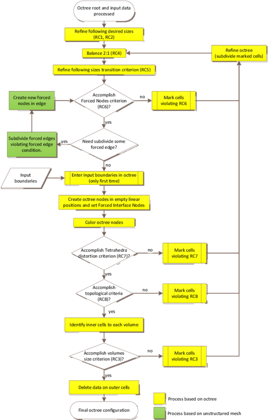
|
| Figure 71: Flowchart of octree refinement process. |
The last step in the octree refinement process is the so called Delete data on outer octree cells. From this point of the meshing algorithm on, the cells of the octree will not be subdivided anymore and only the inner and interface cells are involved in the meshing process, so all the information of the outer cells is deleted in order to save memory. More than this, in the cases where the eight sons of a cell are outer cells, they are deleted, and their father becomes a leaf. This derefinement process may make the octree violate some of the refinement criteria (in particular, the octree may be unbalanced). As the only leaf cells involved in the meshing process are the interface and the inner ones, only these ones must fulfill the refinement criteria.
Concerning the topological refinement criteria (RC8), only the criterion a) has been implemented, which is the one involving tetrahedra edges. The other two criteria (focused on surface and volumetric entities) involve more complex geometric operations which may lead to a more computational expensive algorithm. In order to take them somehow into account, a cheaper refinement criterion has been implemented: it consists in refining a cell if it is an interface cell with no forced node and no edge from the tetrahedra generated from the cell intersects the input boundaries. This criterion is not as restrictive as the whole RC8 one, but it is considerably less computationally expensive. The examples run show that it is fulfilled for most of the cases, specially if a reasonable desired mesh size is provided in the input data. Only some special configurations of boundaries would need a full implementation of the complete RC8 criteria.
6.5.3 Tetrahedra coloring
The tetrahedra coloring algorithm is described in Section 5.3.7, where the Proposition 1 gives a theoretical solution for some configurations of tetrahedra to be colored. However, it only determines the color of the tetrahedron if the continuous curve (with no intersections with the boundaries) between and exists. There are infinite continuous curves in space going from to contained inside the tetrahedron, and infinite positions inside face for point , so a strategy should be used to find the one (if it exists) fulfilling the proposition.
The strategy chosen in the present work is to check between a limited number of curves and points , based on make the algorithm as simpler as possible. Specifically, only straight lines are taken into account, and only a few sample of points are chosen inside face . If some of these chosen curves satisfy the proposition, the tetrahedron can be colored. However, if they do not fulfill the proposition no decision can be taken, because nothing guarantees that there should not be other point with a related curve fulfilling it.
In non-watertight geometries the Proposition 1 should not be applied because there is no guarantee to be valid if some of the curves passes through a gap. In the present work it has been applied also in these cases with the risk of assigning a bad color to a tetrahedron.
We finally mention that in some pathological configurations of tetrahedra, some elements may remain uncolored because no point P chosen fulfills the proposition. In these cases, as a last chance, the color of the tetrahedron is set to the color of its center, which is colored using the standard node coloring process.
6.5.4 Inner surface meshing
As explained in Section 5.3.10, when meshing inner surfaces the triangles corresponding to the mesh of the inner surface must be detected among the faces of the tetrahedra containing nodes on the surface. This process is done just after the tetrahedra coloring process, and involves the following steps:
- Detect all the candidate triangles. The candidate triangles are the ones which all its nodes are forced nodes in interface or in edge, placed on an inner surface.
- Set as valid the topologically right ones. These are the ones accomplishing the topologically properties defined in Section 5.3.10.
- Set as invalid the ones accomplishing the Proposition 2. Not considering the already set as valid, the Proposition 2 is used to set as invalid the corresponding candidate triangles.
- Check the final configuration of triangles. After the previous steps, there can be some configuration not accomplishing the topology of the inner surface. This is, some node which should be manifold belongs to a set of triangles which are not manifold. In these cases a last procedure is performed in order to try to get a final valid mesh. It consists in trying to set as valid some invalid triangle (or set as invalid a valid one), and then check if the topology is accomplished. This is done for the triangles in contact with problematic nodes. Usually after applying the Proposition 2 almost all the triangles are correct and only some local region present topological inconsistencies, so this last strategy often gives good results and solves the local irregularities.
An extra consideration must be taking into account concerning the inner surfaces. As they are surrounded by the same volume (considering the outside part of the domain as volume zero), they do not affect to the coloring of the nodes. For this reason, when computing the intersections of the rays used in that process, the surface entities coming from an inner surface are not considered.
6.6 Parallel processing
The core of the meshing algorithm developed in this work is serial in the sense that the it implies a number of tasks to be done one after another. However, some of these tasks can be parallelized. In the present work shared memory paradigm following OpenMP strategy has been used to parallelize the more costly parts of the algorithm in terms of CPU time. These are the key parts of the algorithm parallelized:
- Nodes coloring. Each one of the rays used to color the nodes it passes through is independent from the others, so the rays are shot in parallel.
- Surface fitting process. Using topological information (the color of the nodes and the cells they belong to), the edges candidates to be affected by the surface fitting process are detected. Then, it has to be checked whether they intersect the input boundaries or not. This process is done in parallel, as each one of the edges are independent from the other ones.
- The checks needed to verify if a cell must be subdivided or not following the refinement criteria RC1, RC2, RC3, RC7 and RC8 only depend on the cell itself and the input boundaries. This allows to treat in parallel the cells to be checked for these refinement criteria.
- Tetrahedra generation through patterns. This process is totally parallel, as the creation of the tetrahedra are independent from each cell and, inside a cell, from each of its faces. Actually, in some configurations the creation of the tetrahedra also depends on the neighbor cell, but in this case it is easy to prioritize which cell generate the tetrahedra (Section 3.3.3). It has to be noted that this process is very fast and only slight differences can be appreciated between the serial and parallel versions of the algorithm.
- Edge collapsing. The edge collapsing process is performed as follows. First of all the detection of edges suitable to be collapsed is performed, ensuring no node of an edge belongs to another edge to be treated. This step is done in serial, but it could be improved including locks in a parallel implementation. Then, in parallel, each edge is checked in order to evaluate if it can be collapsed, and if so, it is collapsed. This process is repeated a number of times in order to ensure that all the edges of the mesh have been taken into account.
- Smoothing process. The smoothing process is performed as follows. First of all, different non overlapping clusters of elements (containing bad quality elements) are detected, and then each one of these clusters is smoothed in parallel only moving its inner nodes. The clusters detection is done in parallel, but is could be improved in a parallel implementation including some locks in the code. This process is repeated a number of times in order to ensure all the nodes have been treated.
The performance of the code could be improved by parallelizing other parts of algorithm. In the present work, only the parts representing a bottle-neck and the ones naturally parallel have been considered for parallelization.
Considering the structure of the octree, a parallelization based on distributed memory can be thought for the algorithm. Briefly explained, the octree cells could be subdivided in different domains, and the whole meshing process could be applied to each part, taking into account to pass the information from one part to the other through the cells interfacing different parts of the domain. This process should be studied in detail and is out of the scope of this work.
6.7 Parameters used
In this section the value of the parameters governing the mesher are detailed.
- (defined in Section 5.3.2, page current). It corresponds to the portion of the octree leaf size to be used as a limit distance. If a node is closer than it to the input boundaries, it is considered forced interface point. is a positive value, and cannot be higher than in order to avoid the creation of inverted tetrahedra due to an excessive distance of the octree nodes with respect to their octree position. In the current implementation takes the value of .
- (defined in Section 5.3.1, page current). It represents the maximum chordal error allowed at the time of creating the forced edges from the forced line entities. The examples run show that the presence of chordal error (even if it is very small) in the forced edges may cause problems at the time to perform the surface fitting operations. For this reason, in the present implementation its value is really low: .
- (defined in Section 5.2.2, page current). This value is used for checking whether a cell must be subdivided or not, considering a desired size in its region. The subdividing process divides by two the size of the resulting children cells. A value of ensures the cell will be subdivided when the size of the resulting children is closer to the desired size than the size of the cell itself. However, in the present implementation a value of have been chosen in order to avoid an excessive level of refinement in some examples.
- (defined in Section 5.3.3, page current). This is a real value between and indicating the percentage of the length of an edge to be use as a limit distance to consider two intersection points in the edge close enough to refine the cell following the topological refinement criterion. The value used in the present implementation is .
- (defined in Section 5.3.5, page current). In the preserving features operations, this parameter controls if the intersection point between a base line entity and the tetra face is close enough to one of the tetrahedra nodes to move the node to its position. It is a percentage of the size of the shortest edge of the tetrahedra (so it must be a value between and ). The value used in this implementation is .
- (defined in Section 5.3.5, page current). This parameter controls if the intersection point between a base line entity and the tetrahedra face is close enough to one of the tetrahedra edges to split it in the preserving features operations. It is a portion of the size of the shortest edge of the tetrahedra (a value between and ). The value used in this implementation is .
- (defined in Section 5.3.6, page current). This parameter is the portion of an edge length to set the limit distance in the surface fitting process used to decide if the edge must be split, or one of the nodes of the edge must be moved to the intersection point. Its value must be compressed between and . A value close to will split all the edges, and a value close to will move the edge nodes in the surface fitting process. The value used in this implementation is .
- (defined in Section 5.3.8, page current). It is the portion of the cell size to set the limit length under which an edge will be collapsed in the make-up operations. A value equal to will not collapse any edge. The value used in the present implementation is .
- (defined in Section 6.3, page current). This parameter controls the distribution of generalized mesh size points onto the mesh size entities. It must take a value greater than one. A value equal to one would create too much generalized mesh size points, and a value greater than two could leave areas in the mesh size entity not covered by any generalized mesh size point. The value used in this implementation is , considering the region of the octree cells affected by a mesh size entity is always larger than the mesh size entity itself.
- (defined in Section 3.4, page current). It is the portion of the model bounding box size used to create the MIPs when more than one intersection point are very close one from each other. It must be a very low value not to collapse relevant details of the model when dealing with the pathological intersections situations. The value used in the present implementation is .
7 Examples
In this chapter some examples of meshes generated using the proposed algorithm are shown. In the first part, some simple validation examples are shown in Section 7.1. These examples try to demonstrate the effectiveness of the mesher in dealing with some of the typical drawbacks of octree based meshers (mainly geometrical features and topological preservation), so they do not involve large meshes.
Examples in Sections 7.2 and 7.3 involve complex real geometries trying to evaluate the performance of the new meshing algorithm for complicated geometries and the generation of a large amount of elements.
The analysis of the results considering all the representative examples is carried out in Section 7.4. Some representative cases are used in Section 7.4.1 to compare the prefomance of the new mesher with other two meshers:
- An advancing front implementation (the one included in the GiD v11 version [56,57,58]).
- A Delaunay implementation (the one provided in Version 1.4 of the Tetgen library [61]).
In order to present a realistic view of the results and allow their correct evaluation, the following data of the model to be meshed is provided for each example:
- Sphericity of the model (S). The specific surface of a solid (volume) is computed as the ratio between the area of its surfaces and its volume. Its units are of . This ratio is useful to asses the speed of tetrahedra generation. In the presented method the tetrahedra within the volumes are extremely fast to generate, and the most time consuming operations are related to the tetrahedra near the boundary. The more specific surface has the model, the more expensive (in computational terms) the mesh generation will be. However, the specific surface measure is not dimensionless. For instance, scaling homogeneously a volume changes its specific surface, so this measure is not suitable for comparing models with different sizes.
To be able to compare different models (with different sizes), the sphericity is provided instead of the specific surface. This measure is dimensionless, and indicates how far is the volume measured from a sphere (which is the shape with less specific surface enclosing a given volume). The sphericity of a model is computed using the following equation:
|
|
(7.1) |
where is the volume of the model and is the area of the surface entities defining the domain. The sphericity takes values from (shapes with high specific surface) to (a perfect sphere). Theoretically, the presented algorithm should be faster for models with higher sphericity.
- Input mesh size. Some of the examples are meshed with a uniform mesh size, and some of them have different desired mesh sizes assigned to different parts of the domain. The desired mesh sizes of each example are detailed.
- Number of volumes present in the model.
- Number of surface entities in the input boundary. In all the examples shown these are triangle mesh elements. This can give an idea of a ratio between the input boundary entities size in comparison to the octree leaves (which are more less of the same size of the final mesh elements).
- Watertight condition. If the model is watertight or not.
- List of the relevant general parameters used for the mesher (Section 3.1).
For each case, some figures of the input boundaries and the final mesh are shown as well as the following data:
- Number of nodes generated.
- Number of tetrahedra generated.
- Number of triangles in the final mesh (faces of tetrahedra interfacing different volumes).
- Number of line elements (coming from forced edges) in the final mesh.
- Quality of the elements generated. In order to distinguish between the mesher itself and the make-up and smoothing operations, the quality of the elements will be shown before and after these operations. The minimum dihedral angle of the element is taken as a quality measure, and its accumulated distribution among all the elements is provided. The value corresponding to the worst quality element of the mesh is also provided, as well as the number of elements with a minimum dihedral angle lower than degrees (in case there are some).
- Memory used by the algorithm. The memory needed to store a given mesh can be determined a priori, as it consists of the coordinates of the nodes and the connectivity of the elements. However, during the mesh generation process, extra memory is needed to store auxiliary data. These data are deleted once the mesh has been generated. The ratio between the peak of memory needed to generate the mesh and the memory required to store that mesh is given in order to evaluate the efficiency (in terms of memory) of the implementation of the algorithm. A value of this ratio higher than one is expected, as the algorithm should consume more memory for generating the mesh than the needed to store it (once it has been generated).
- Time needed to generate the mesh. The time of the whole mesh generation process is given, as well as the time consumed by the different parts of the algorithm, to allow the evaluation of possible bottle necks. As the implementation of the algorithm has been done following parallel processing techniques, in the relevant examples the time will be provided taking into account different scenarios: using only one thread (as a reference time), and using two, three and four threads. This allows to evaluate the scalability of the algorithm. The time is measured using the function [62], and the value provided is the mean among five measures taken.
- Speed: number of tetrahedra generated per minute. This speed is provided in order to compare with other methods, but it has to be taken into account that it can lead to misleading evaluations because of the sphericity considerations mentioned above. Another important factor to be considered when assessing the tetrahedra generation speed is the mesh desired size in comparison with the final sizes of the mesh. Specially in the operations needed to preserve the volume topology, the algorithm is more time-consuming if it has to refine automatically than if the sizes introduced by the user fulfill directly the topological criteria.
- Speed-up: the speed-up is defined as the ratio between the time needed to run a process in serial and the time needed to run it in parallel (using more than one thread). This value is given in the examples run in parallel, in order to evaluate the efficiency in the parallel implementation of the algorithm.
In order to evaluate the efficiency and performance of some parts of the algorithm as well as their implementations, the following data is also provided:
- Number of local ray castings performed: local ray casting operations are needed in the coloring algorithm when the three Cartesian rays incident to a node are invalid. The number of local ray casting operations performed provides an idea of the robustness of the coloring algorithm presented in this work.
- Number of undetermined tetrahedra: these are the ones colored following the tetrahedra coloring algorithm explained in Section 5.3.7.
- Number of tetrahedra in interface cells: as explained in Section 6.5, almost all the operations of the mesher are applied to the tetrahedra generated from interface cells, and the tetrahedra from the inner cells of the volumes are not generated until the end of the meshing process. The number of tetrahedra in interface cells gives an idea of the memory saved during the meshing process thanks to the fact that the tetrahedra from the inner octree cells are not generated yet. Two values are provided:
- The number of tetrahedra generated directly from the interface cells applying the tetrahedra pattern.
- The number of tetrahedra just after the make-up and smoothing operations. This number results from applying to the previous one the operations of preserving geometrical features, surface fitting operations, deleting the outer tetrahedra and performing the make-up and smoothing operations.
- Number of octree cells. The total number of cells of the octree is provided (as well as the number of interface and outer cells) considering the refinement criteria in the whole octree root. Also the total number of cells not applying them to the outer cells is provided in order to give an idea of the memory saved thanks to the presented implementation.
The characteristic sizes, as well as the mesh sizes of the examples are expressed in general units of length (uol).
All these data are not provided in all the examples, as each one of them has specific results to be highlighted, so only its relevant data will be provided. Complete tables of the data for all the examples studied in this chapter are available in Appendix 9.
The meshing algorithm has been implemented as a library, and it has been integrated in the pre and post-processor GiD [56,57,58]. The examples shown in this document are meshes using the version of the algorithm present in the 11.1.9d version of GiD, which can be downloaded from the website [63]. All the meshes have been generated in a computer with the characteristics shown in Table 4.
| Processor | Intel Core i5 3570K @3.40GHz |
| RAM memory | 32.0 GB DDR3 800 MHz |
| OS | Windows 8 64-bits |
The code is written in C++ and it has been compiled using Microsoft Visual Studio 2012 Version 10.0.402191.1 SP1Rel with OpenMP enabled [62].
7.1 Validation examples
In this section, some validation examples are shown. Some of them have been chosen in order to demonstrate that the presented mesher can generate meshes from input data which is not treatable in raw by other volume meshing techniques (like advancing front or Delaunay). This is the case for non-watertight input boundaries, or input triangle meshes with very low quality elements. Other examples may be more suitable to be meshed with these techniques, but they have been used to demonstrate that the presented algorithm solves some common problems in octree based methods (like the preservation of topology or geometric features).
7.1.1 Preserving topology
As mentioned in Section 2.5, one of the disadvantages of the octree-based meshers is the difficulty to preserve the topology of the model. Some examples are presented in this section showing that the proposed algorithm solves this problem. The combination of the topology refinement criterion, the surface fitting process and the tetrahedra coloring are the main parts of the algorithm in charge of preserving the topology.
Some of these examples may be obvious to be meshed using other techniques like advancing front or Delaunay based meshers, but this is not the case for classical octree-based meshers.
7.1.1.1 Validation example VE-T1
The first example is the one shown in Figure 72. This model is formed by an axisymmetric watertight volume. It has no geometrical features to be preserved and all its surfaces are curved. The particularity of the model is that its central part is very thin in comparison with its characteristic size. A view of the geometrical model (represented with NURBS surfaces) is shown in Figure 72(a), where its characteristic sizes are depicted. The contour mesh of the volume used as the input boundaries for the volume mesher is shown in Figure 72(b).

|
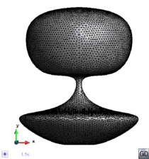
|
| (a) | (b) |
| Figure 72: Model used in the validation example . (a) View of the geometry of the volume and its characteristic sizes. (b) View of the triangle mesh used as the input boundaries for the volume mesher. | |
In this example no desired mesh size has been set in the input data, and a size transition factor () equal to has been used. This is the most unfavorable situation for the mesher, as it implies that all the octree refinement process is based on the topology criteria and the constrained two to one condition given by the balance criterion.
| ||||||
| Figure 73: Results for the validation example . (a) View of a cut of the octree cells after the refinement process and part of the input boundaries. (b) Final tetrahedra mesh generated. (c) Mesh generated if the tetrahedra coloring is based on the color of the center of each element. |
A view of the octree cells in a cut plane passing trough the rotation axis of the model is shown in Figure 73(a). This configuration of cells is the result of applying the octree refinement process to the octree root. It can be seen that, even when no desired mesh size has been assigned, the octree is refined because of the topology criteria.
The final mesh is depicted in Figure 73(b). It is a very coarse mesh, as no mesh size was entered in the input data. However, it represents perfectly the topology of the model. In this case, the tetrahedra coloring strategy plays a key role for preserving the topology. The use of the simple tetrahedra coloring technique based on assigning to each element the color of its center would yield the mesh shown in Figure 73(c). It can be seen that the model topology would not be preserved using such simple tetrahedra coloring technique, as the upper and lower parts of the model would be connected by just one node in a non-manifold way.
Although the mesh generated in example accomplish with the requirements of the mesher, the elements are too large to capture reasonably well the shape described by the input boundaries. Hence, it may not be useful for a given numerical simulation. A mesh of the same model with a desired mesh size of uol is depicted in Figure 74(a) in order to empathize that the mesher is flexible in terms of mesh size assignment: if no mesh size is entered in the input data, a legal mesh is generated, but if some specific mesh size is needed, the mesher takes care of it. A view of the inner elements is depicted in Figure 74(b). The regular distribution of elements coming directly from the tetrahedra patterns from the octree cells can be appreciated in the inner parts of the volume.
| ||||||
| Figure 74: Results for the validation example with mesh size equal to uol. (a) Final tetrahedra mesh generated. (b) View of the inner elements of the mesh. (c) Mesh generated if no topological mesh refinement criterion is applied. It can be seen that the topology of the model is not preserved in this case, as there are two unconnected parts of the final mesh |
The data of the generated mesh is detailed in Table 5.
| Number of threads | |
| Mesh size (uol) | |
| Number of tetrahedra | |
| Number of nodes | |
| Minimum dihedral angle (degrees) | |
| Time to generate the mesh (seconds) | |
| Speed (Mtetrahedra per minute) |
It has to be noted that, decreasing the desired mesh size, the resulting mesh fits much more with the original shape of the domain. However, even with a mesh size of uol, the classical approach for octree based meshers would generate an invalid mesh like the depicted in Figure 74 (c). This is because the size of the cells is larger than the thin part of the model. In this situations it is crucial to use a strategy for the octree refinement and a surface fitting process able to preserve the topology of the model. In the case of the presented mesher the refinement criteria takes into account the posterior surface fitting process.
7.1.1.2 Validation example VE-T2
The validation example (Figure 75) also presents some thin parts. In this case the model is formed by 4 watertight volumes: the upper part, the lower part and the two cylindrical parts connecting both. The extreme surfaces of the cylindrical volumes are shared by two volumes. As it can be seen, this model has sharp edges to be preserved by the mesher.
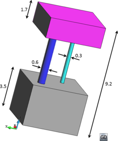
|
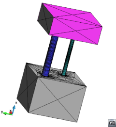
|
| (a) | (b) |
| Figure 75: Model used in the validation example . (a) View of the geometry of the model and its characteristic sizes (in uol). Different volumes are drawn in different colors. (b) View of the triangle mesh used as the input boundaries for the volume mesher. | |
Analogously as the validation example , no desired size has been provided to the mesher and is equal to , so the refinements needed to preserve the topology of the original model are performed automatically by the mesher.
The tetrahedral mesh generated is shown in Figure 76(a). As it can be seen, the topology of the model has been preserved, as well as its sharp edges. Each volume of the model has its corresponding tetrahedra, and they fit the contour surfaces. A zoom view of the inner elements is shown in Figure 76(b).
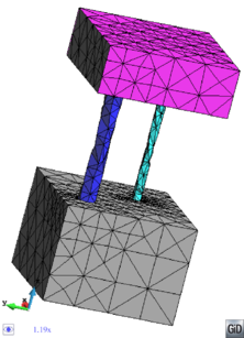
|
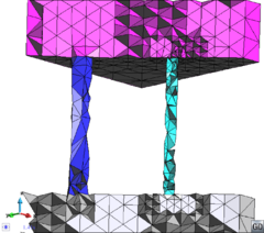
|
| (a) | (b) |
| Figure 76: Results for the validation example . (a) Final tetrahedra mesh generated. (b) Zoom view of some internal elements of the final mesh. | |
The data of the generated mesh is detailed in Table 6.
| Number of threads | |
| Mesh size (uol) | |
| Number of tetrahedra | |
| Number of nodes | |
| Minimum dihedral angle (degrees) | |
| Time to generate the mesh (seconds) | |
| Speed (Mtetrahedra per minute) |
No mesh size has been provided to the mesher in order to check the preservation of the topology of the model by the mesher. While the topology has been perfectly captured, the element size in the thin parts of the model is too large to define properly the curved shape. These elements have a high chordal error, which is a typical weak point of the octree based meshers. Nevertheless, assigning a smaller size in the curved regions a better quality mesh is obtained as shown in Figure 77. Some specific make-up and smoothing operations may also reduce the chordal error of the mesh.
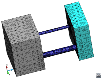
|
| Figure 77: View of a mesh of the validation example with a smaller mesh size in the curved parts of the domain. |
In this example the independence of the mesh generator to the input mesh quality is demonstrated. In Figure 75(b) it can be appreciated that the boundaries of the volumes are well defined in terms of chordal error, but the quality of the triangles is very low. However, this does not affect the meshing algorithm. In methods based on the advancing front technique, the input boundaries of this example could not be used directly as the active front for the volume meshing. A previous mesh improvement of this input surface mesh should be required, or even the generation of a new one. In the other hand, this provides the advancing front methods with a better mesh quality in terms of chordal error.
7.1.1.3 Validation example VE-T3
As the topology refinement criteria concerning surfaces and volumes ((b) and (c)) are not implemented, the more unfavorable case for the presented algorithm is the one where the model has very thin parts, understanding thin as a distance much smaller than the bounding box of the domain. In these situations, the octree only will be refined properly to capture the topology of the model if some of the edges of the tetrahedra generated from the cells intersects the input boundaries. If not, the octree should be too coarse and the surface fitting process should not be able to capture well the boundaries.
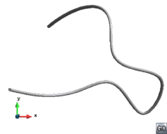
|
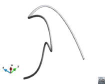
|
| (a) | (b) |
| Figure 78: Model used in the validation example . Two views ((a) and (b)) of the triangle mesh used as the input boundaries for the volume mesher are shown in order to get a proper 3D perception of the geometry. The diameter of the cylindrical volume is uol, and the side of its bounding box is around uol. | |
This validation example corresponds to this unfavorable situation. A view of the model and the input boundaries used to feed the mesher is shown in Figure 78. The model is a unique watertight volume representing a cylindrical rod curved in space. The diameter of the cylinder is uol, and the bounding box of the model is around uol.
A mesh with a mesh size of has been generated using the presented algorithm. The final mesh is shown in Figure 79. It can be appreciated that the topology of the model is preserved. The data of the generated mesh is detailed in Table 7.
| Number of threads | |
| Mesh size (uol) | |
| Number of tetrahedra | |
| Number of nodes | |
| Minimum dihedral angle (degrees) | |
| Time to generate the mesh (seconds) | |
| Speed (Mtetrahedra per minute) |
| ||||||
| Figure 79: Result mesh of the validation example . Different views of the mesh generated with a desired mesh size of uol. |
A mesh generated with no mesh size assigned (which is the most unfavorable situation for the mesher) is shown in Figure 80(a). As commented above, the no implementation of the surface and volumetric parts of the topological refinement criterion can lead to situations where a cell does not recognize the need to be subdivided. This occurs in this case. It can be appreciated that the topology of the model has not been preserved, as there are parts of unconnected meshes representing the unique volume of the model. This example shows the importance of the topology refinement criteria.
A view of the octree refined merged with the input boundaries is depicted in Figure 80(b). Although the octree is relatively refined in the regions where the volume is, the level of refinement is not enough to let the surface fitting process capture well the topology of the model. It can be seen that the octree is more refined in the end parts of the volume. This is due to the presence of sharp edges there, so the corresponding forced edges are created. They involve forced points which activate the forced nodes refinement criterion.
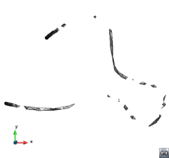
|
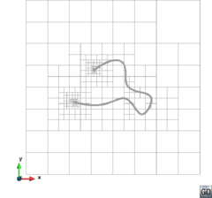
|
| (a) | (b) |
| Figure 80: Mesh of the validation example with no mesh size assigned. (a) View of the tetrahedra mesh generated. Note that the topology of the model is not preserved in this case. (b) View (aligned with a Cartesian direction) of the octree merged with the input boundaries. | |
It is uncommon not to provide with any characteristic size of the model at the time of generating a mesh for a numerical simulation. Due to the solver needs or for the need of accuracy in the shape representation, often a size is provided to the mesher locally or globally in order to reach a successful mesh for the simulation. Actually, in the presented case it can be appreciated that the mesh obtained with a mesh size of uol (although it preserves the topology) may be too coarse to represent the curvature of the rod with an acceptable chordal error. A zoom view of a mesh of the same example using a mesh size of uol is depicted in Figure 81. It can be seen that the chordal error of the mesh is considerably reduced.
One remark to be done is that the assignment of sizes can be done manually or automatically. In this example an automatic size could be assigned to the input boundaries considering the curvature of the model, so no user interaction should be needed.
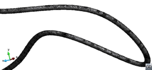
|
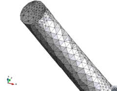
|
| (a) | (b) |
| Figure 81: Zoom views of a mesh of the validation example with a mesh size of uol. | |
7.1.2 Preserving geometrical features
Two validation examples are presented in this section in order to check the preserving of geometrical features: corners and ridges.
7.1.2.1 Validation example VE-F1
This validation example is shown in Figure 82, where its characteristic sizes are depicted. It is a synthetic wing profile.
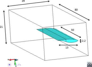
|
| Figure 82: Model used in the validation example . View of the geometry of the model and its characteristic sizes (in uol). |
Computational Fluid Dynamic (CFD) simulations of this kind of geometries require to capture the flow behavior near the end part of the wing (the sharp edge), so its preservation is crucial for the mesher. Two views of the input boundaries used for the mesher are depicted in Figure 83.
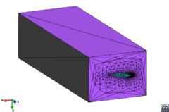
|
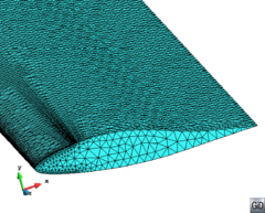
|
| (a) | (b) |
| Figure 83: Views of the triangle mesh used as the input boundaries for the validation example . (a) View of the the outer part of the control volume. (b) Detail of the triangle mesh in the wing profile used as input boundaries. | |
The model has a control volume around the wing profile and two volumes are meshed: the wing itself and its outer part (inside the control volume). The two volumes are watertight. A size of uol has been assigned to the surface entities of the wing, and the is equal to . The general mesh size for the control volume is uol.
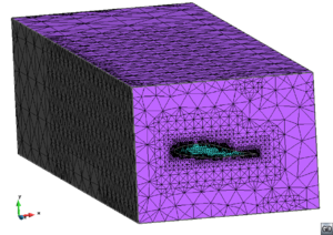
|
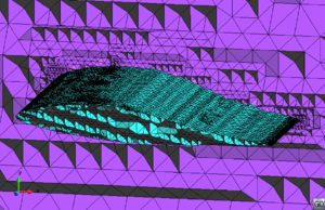
|
| (a) | (b) |
| |
| (c) | |
| Figure 84: Results for the validation example . (a) Final tetrahedra mesh. (b) and (c) Zoom views of internal elements of the final mesh. | |
The tetrahedra mesh generated is shown in Figure 84(a). A zoom view of the inner elements is shown in Figure 84(b). As it can be seen, the sharp edges have been properly preserved. It also can be appreciated that the size of the skin triangles of the generated tetrahedra is independent from the size of the triangles of the input boundaries. The independence of sizes between the input and the final mesh is an advantage of the presented meshing algorithm: the mesh of the input boundary only has to take care on criteria for representing precisely the shape of the domain, without considering the required size for the volume mesh. The same input boundary mesh can be used for generating volume meshes with different sizes. In advancing front-based meshers, for instance, the surface mesh has to be generated for each new size required for the volume.
The data of the generated mesh is detailed in Table 8.
| Number of threads | |
| Mesh general size (uol) | |
| Mesh size in the wing surface (uol) | |
| Transition factor | |
| Number of tetrahedra | |
| Number of nodes | |
| Minimum dihedral angle (degrees) | |
| Number of tetrahedra with minimum dihedral angle lower than degrees | |
| Time to generate the mesh (seconds) | |
| Speed (Mtetrahedra per minute) |
It can be appreciated that the minimum dihedral angle of the mesh elements is degrees, and there are three elements with a minimum dihedral angle less than degrees. These elements are in the wing volume, in the region where the geometry itself have a very small dihedral angle (the rear part of the wing).
7.1.2.2 Validation example VE-F2
The validation example is the model of a mechanical piece (a crankshaft of an automotive) provided by the company Quantech ATZ [64]. Its geometrical definition comes from an .stl file (that is, a triangle mesh). This triangle mesh representing the input boundaries (depicted in Figure 85) is watertight.
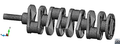
|
| Figure 85: Model used in the validation example . View of the triangle mesh used as the input boundaries of the volume. |
The dimensions of the bounding box of the model are around by by uol. The thin parts of the model have approximately uol. A uniform mesh size of uol and a equal to has been provided in the input data of the mesher.
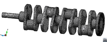
|
| Figure 86: Results for the validation example . Final tetrahedra mesh generated. |
The tetrahedra mesh generated is shown in Figure 86. As it can be seen, the sharp edges have been properly preserved. Some zoom views of the mesh and the inner elements are depicted in Figure 87.
| |||
| Figure 87: Different views of the mesh generated from validation example and its inner elements. |
It has to be noted that the input boundaries in this example are defined with very low quality triangles. However, the new mesher does not need a good quality mesh to represent the boundaries of the domain. This is not the case for other meshing algorithms, like the one based in advancing front technique. Using such techniques with this model would require a previous meshing of the boundaries, even when the domain is watertight (like in this case).
The data of the generated mesh is detailed in Table 9.
| Number of threads | |
| Mesh general size (uol) | |
| Transition factor | |
| Number of tetrahedra | |
| Number of nodes | |
| Minimum dihedral angle (degrees) | |
| Number of tetrahedra with minimum dihedral angle lower than degrees | |
| Time to generate the mesh (seconds) | |
| Speed (Mtetrahedra per minute) |
7.1.3 Non-watertight boundaries
Some validation examples are presented in this section with non-watertight volumes. When dealing with non-watertight geometries, it is not guaranteed that any edge of the mesh or any ray of the ray casting operations passes through a gap or a region with overlapping entities. To validate the algorithm, the models used in the first two examples have been created ensuring that some of these situations happens.
It has to be considered that these examples cannot be meshed using advancing front or Delaunay based techniques, as they require a watertight definition of the boundaries of the domain. In these cases, an extra effort must be invested in the CAD cleaning operations, or even to re-gerenate the mesh of the boundary surfaces before applying the volume mesher.
7.1.3.1 Validation example VE-W1
This example consists in a cubic volume with a gap in one of its faces. A view of its geometry with its characteristic sizes and the triangle mesh used as input for the mesher is shown in Figure 88.
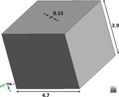
|
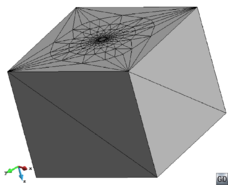
|
| (a) | (b) |
| Figure 88: Model used in the validation example . (a) View of the geometry of the volume and its characteristic sizes in uol. (b) View of the triangle mesh used as the input boundaries for the volume mesher. | |
The position of the gap (centered in the face) ensures that some of the rays used in the ray casting technique, as well as some tetrahedron edge involved in the surface fitting process passes through it.
The model has been meshed with a uniform mesh size of uol and a equal to . It has to be noted that, when dealing with input boundaries with gaps, the mesh size in the region of gap must be greater than the gap itself, otherwise the mesher could fail.
The tetrahedra mesh generated is depicted in Figure 89. It can be appreciated that the skin of the mesh is completely watertight, closing the gap existing in the input boundaries. In the coloring process, the Cartesian ray passing through the gap has been considered as invalid, but the contributions of the other ones have provided with the right information in order to color all the nodes. In the surface fitting process some GIPs (Section 3.4.1) have been generated, as some of the edges of the tetrahedra mesh passed through the gap.
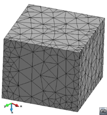
|
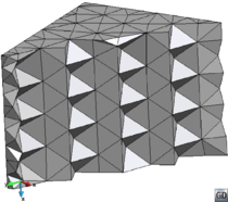
|
| (a) | (b) |
| Figure 89: Results for the validation example . (a) Final tetrahedra mesh generated. (b) View of internal elements of the final mesh in the region where the gap in the input boundary is. | |
The data of the generated mesh is detailed in Table 10.
| Number of threads | |
| Mesh general size (uol) | |
| Transition factor | |
| Number of tetrahedra | |
| Number of nodes | |
| Minimum dihedral angle (degrees) | |
| Time to generate the mesh (seconds) | |
| Speed (Mtetrahedra per minute) |
7.1.3.2 Validation example VE-W2
This validation example aims to evaluating the mesher in non-watertight geometries having overlapping entities in its contours.
For this purpose, a model of an sphere has been build from two different skin meshes of the same sphere with a slight difference in its mesh size. Some elements of the meshes have been deleted, and then both triangle meshes have been merged.
| ||||||
| Figure 90: Model used in the validation example . (a) The input boundaries are built merging two different parts of triangles meshes of a sphere (shown in (b) and (c)), so it has overlapping surface entities. |
The two different meshes used (depicted in different colors), as well as the resulting boundary of the sphere are shown in Figure 90. It can be appreciated the overlapping regions in some parts of the boundaries. Actually, there are regions where one of the sphere skins is in the outer part of the domain, and regions were it is in the inner part. It has to be noted that the two skin meshes are not intersected: they have no topological relationship although they are occupying the same position in the 3D space.
The radius of the sphere is uol, and the maximum distance between overlapping entities is around uol. The mesh has been generated with a uniform size of uol.
The tetrahedra mesh generated is depicted in Figure 91. It can be appreciated that the skin of the mesh is completely watertight and enclose the volume of the sphere correctly.
The data of the generated mesh is detailed in Table 11.
| Number of threads | |
| Mesh general size (uol) | |
| Transition factor | |
| Number of tetrahedra | |
| Number of nodes | |
| Minimum dihedral angle (degrees) | |
| Number of tetrahedra with minimum dihedral angle lower than degrees | |
| Time to generate the mesh (seconds) | |
| Speed (Mtetrahedra per minute) |
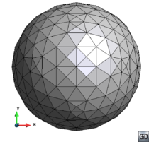
|
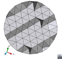
|
| (a) | (b) |
| Figure 91: Results for the validation example . (a) Final tetrahedral mesh. (b) View of internal elements of the mesh. | |
7.1.3.3 Validation example VE-W3
The model used for this validation example is a mechanical part (one volume) provided by the company Quantech ATZ [64]. Its definition comes directly from a CAD system in mesh format (.stl) as it is provided in some real industry applications. As it is common in these cases, the input boundaries are non-watertight, although the geometrical definition (with NURBS surfaces) was watertight in the original CAD system used to define its shape. It is a very common case which illustrates the need of CAD cleaning operations before the meshing process when a conventional volume mesher is used. This example evidences that this meshing algorithm works without the need of performing any CAD cleaning operation.
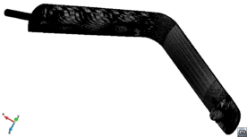
|
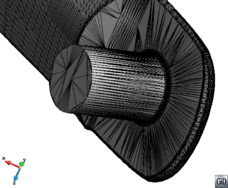
|
| (a) | (b) |
| Figure 92: Model used in the validation example . (a) Render view of the contours of the volume. (b) Zoom of a part of the contours with the sharp edges to be preserved. | |
A view of the model is depicted in Figure 92. It can be seen that some of the triangles used for the definition of the boundaries have a very bad aspect ratio. However, the shape of the volume is represented very well (with very low chordal error). The model boundary is smooth, but some parts of it (the cylindrical parts) present sharp edges to be preserved, as shown in Figure 92(b). The largest size of the bounding box of the model is around uol, and the thin parts of it measure around uol. The general desired mesh size used is uol.
Defining the higher entity index of an edge as the number of triangles it belongs to, the present model has some edge with higher entity index equal to one and four. It has to be noted that a watertight volume must have all the edges of the triangles defining its contour with a higher entity index equal to two. This indicates that the model used in this example is not watertight. The edges with a value equal to one are related to a gap in the contours.
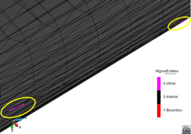
|
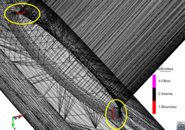
|
| Figure 93: Higher entities indices of the edges of the contours defining the model of . Two zoom views of some of the edges with higher entity index different from two. | |
The higher entity index of the contours of the model is depicted in Figure 93. It can be appreciated that the non-watertight parts of the model are localized in very small regions. This evidences the difficulty of the CAD cleaning operations when a conventional mesher is used: apart from the difficulty to close the gaps of the boundary or edit it to avoid overlapping entities, it may be also difficult to detect the problematic regions. Furthermore, the quality of the triangles representing the input boundaries is very bad, so a new contour mesh should be generated for some standard meshing techniques, such as the advancing front.
The edges of the input boundaries selected to be preserved are the ones enclosing a dihedral angle lower than degrees. Actually, not all of them have been considered, because some of the triangles defining the domain are so distorted that it is not possible to compute accurately its normal (this aspect is more detailed in Section 5.3.1.1). The edges considered to be preserved are the ones of the top of the small cylindrical parts of the volume (Figure 92(b)).
A mesh of uol uniform size has been generated. The data of the generated mesh is detailed in Table 12, and some views of it are shown in Figure 94.
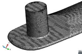
|
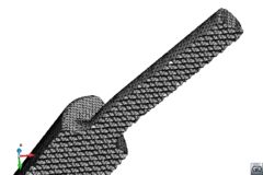
|
| (a) | (b) |
| Figure 94: Mesh generated of the model of . (a) Zoom view of a part of the model. (b) Zoom of a selection of inner tetrahedra. | |
| Number of threads | |
| Mesh general size (uol) | |
| Transition factor | |
| Number of tetrahedra | |
| Number of nodes | |
| Minimum dihedral angle (degrees) | |
| Number of tetrahedra with minimum dihedral angle lower than degrees | |
| Time to generate the mesh (seconds) | |
| Speed (Mtetrahedra per minute) |
7.1.4 Coloring pathological situations
Some validation examples presenting the pathological situations for the ray casting technique detailed in Section 4.2 are shown in this section. The models used are prepared ensuring some of the rays used in the ray casting technique for the nodes coloring intersects the input boundaries in special intersection types (, , or ) creating a MIP (Section 3.4).
7.1.4.1 Validation example VE-C1
The validation example is created repeating a symmetric configuration of volumes ensuring some of the rays of the ray casting process intersects the input boundaries in a MIP with multiple interfaces ( type intersection) and in co-planar intersections ( type intersection).
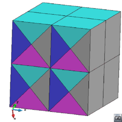
|
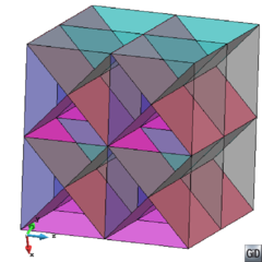
|
| (a) | (b) |
| Figure 95: Model used in the validation example . (a) Render view of the contours of the volumes. (b) Transparent view of the external contours of the model in order to appreciate the inner part of it. | |
The model is shown in Figure 95. It is formed by watertight volumes sharing the contact surfaces between them. The side of the bounding box of the model has uol.
The tetrahedra mesh generated using a general mesh size of uol is depicted in Figure 96. For the node coloring process, no ray has been declared as invalid, so the strategies used for detecting and solving the pathological configurations of rays have been demonstrated to work properly. In particular, intersection types have been involved in this model. This kind of intersections forces to create extra rays from the multiple interface intersection, so more rays are used compared to the single intersection types.
It can also be appreciated that the topology of the model has been correctly represented by the final mesh, as each one of the volumes of the model has its tetrahedra mesh.
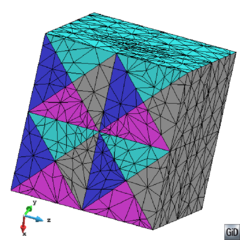
|
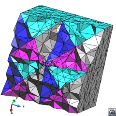
|
| (a) | (b) |
| Figure 96: Results for the validation example . (a) Final tetrahedral mesh. (b) View of internal elements in the final mesh. | |
The data of the generated mesh is detailed in Table 13.
| Number of threads | |
| Mesh general size (uol) | |
| Transition factor | |
| Number of tetrahedra | |
| Number of nodes | |
| Minimum dihedral angle (degrees) | |
| Time to generate the mesh (seconds) | |
| Speed (Mtetrahedra per minute) |
7.1.4.2 Validation example VE-C2
A coil shaped volume has been used for this example. The model is formed by the watertight volume shown in Figure 97, where its characteristic sizes are depicted.
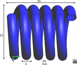
|
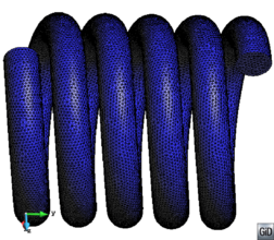
|
| (a) | (b) |
| Figure 97: Model used in the validation example . (a) View of the geometry of the volume and its characteristic sizes in uol. (b) View of the triangle mesh used as the input boundaries for the volume mesher. | |
A large amount of rays used for the nodes coloring of this model intersect tangentially the input boundaries, so it is a suitable validation example to check if the intersection types are well detected and solved.
This model is also interesting from the topology preservation point of view, as the same volume is curved, and some of its parts are very near one from each other. This situation is problematic for many octree based meshers, because they tend to join the parts of the input boundaries which are very close one from each other. This is the case of the mesh depicted in Figure 99.
The tetrahedra mesh generated using the proposed mesher with a desired mesh size of uol is shown in Figure 98. It can be appreciated that all the nodes are colored correctly. Furthermore, the topology of the model is also well captured, thanks to the combination of octree refinement, surface fitting and tetrahedra coloring strategies followed by the presented algorithm.
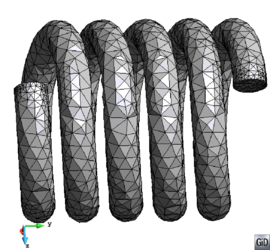
|
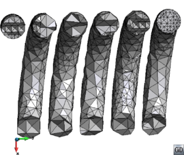
|
| (a) | (b) |
| Figure 98: Results for the validation example . (a) Final tetrahedral mesh. (b) View of internal elements in the final mesh. | |
As in other examples presented, the mesh size chosen in this example is set in order to highlight some feature of the mesher (in this case, the preservation of the topology), but it yields a mesh with a high chordal error in the boundaries due to their curvature. This problem can be solved by just assigning a lower size in the boundaries, as it is shown in Figure 100(b). Some specific make-up and smoothing operations could be also applied to the coarse mesh in order to reduce its chordal error.
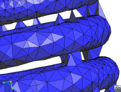
|
| Figure 99: View of a mesh generated with a conventional octree based mesher not preserving the topology of the model. |
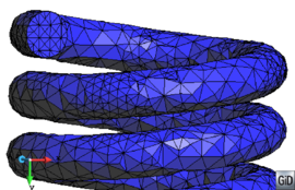
|
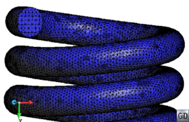
|
| (a) | (b) |
| Figure 100: Zoom view of two meshes of the validation example : (a) with a general mesh size of uol, and (b) with a mesh size of uol assigned to the input surface entities. It can be appreciated the lower chordal error using a lower mesh size. | |
The data of the generated mesh is detailed in Table 14.
| Number of threads | |
| Mesh general size (uol) | |
| Transition factor | |
| Number of tetrahedra | |
| Number of nodes | |
| Minimum dihedral angle (degrees) | |
| Time to generate the mesh (seconds) | |
| Speed (Mtetrahedra per minute) |
7.1.4.3 Validation example VE-C3
This validation example has been created to evidence the local ray casting technique is necessary. This technique is applied when the three Cartesian rays passing through a node are invalid. The model is a cube of uol of side which faces are represented by unconnected triangles in the configuration depicted in Figure 101. The gap size in the center part of the faces is approximately of uol.
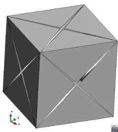
|
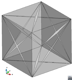
|
| (a) | (b) |
| Figure 101: Model used in the validation example . (a) Render view of the triangle mesh used as input boundary for the mesher. (b) Transparent view in order to appreciate the gaps in the rear faces of the volume. | |
This configuration ensures the node placed in the center of the cube will have its three rays invalid, so its coloring must be made by the local ray casting technique.
The tetrahedra mesh generated with a mesh size of uol is depicted in Figure 102. It can be appreciated that the mesh has been generated successfully, providing with a watertight skin of the tetrahedra. The color of the central node of the cube has been provided using the local ray casting technique, as the three rays passing through it were considered as invalid.
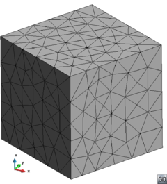
|
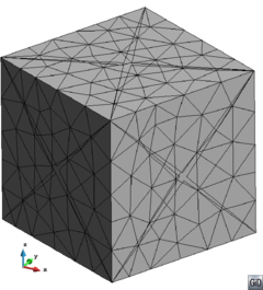
|
| (a) | (b) |
| Figure 102: Results for the validation example . (a) View of the final tetrahedral mesh. (b) The same view of the tetrahedra mesh with the input boundary mesh superposed. | |
The data of the generated mesh is detailed in Table 15.
| Number of threads | |
| Mesh general size (uol) | |
| Transition factor | |
| Number of tetrahedra | |
| Number of nodes | |
| Minimum dihedral angle (degrees) | |
| Time to generate the mesh (seconds) | |
| Speed (Mtetrahedra per minute) |
7.1.5 Surface mesh inner to a volume
In this section an example corresponding to the meshing of surfaces inner to a volume is shown (Section 5.3.10).
7.1.5.1 Validation example VE-I1
This validation example corresponds to a 420 dinghy boat sails set (main, jib and spinnaker). The example includes the mast and other line elements such as the jib halyard, the spinnaker pole and the topping lift. Other elements of the rig such as the shrouds and spreaders have been omitted.
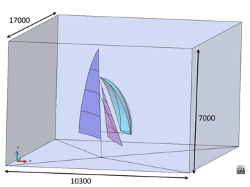
|
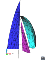
|
| (a) | (b) |
| Figure 103: Model used in the validation example . (a) Render view of the model with transparencies in the outer surfaces of the control volume. Characteristic sizes of the model are depicted in uol. (b) Zoom view of the triangle and linear meshes (used as input boundaries for the mesher) of the sails and the inner line entities to be preserved. | |
From the mesher point of view, the interest of this model is to reach a volume mesh surrounding the sails, and topologically connected to them. Furthermore, the tetrahedra mesh must be also conformal to the line elements (as the mast) present in the model. This means some of the tetrahedra faces should be triangles of the sails, and some of the tetrahedra edges must be 1D linear elements of the model. For this reason a control volume has been built around the model. A view of the model is depicted in Figure 103. From the topological point of view it is interesting to note that the surface entities representing the sails and the line entities representing the other elements are not part of the boundaries of the control volume. They are inside the volume, but with no topological connection to it.
The mesh has been generated with uol as general mesh size, and no specific size assigned to the boundaries. Two different views of the mesh generated are depicted in Figure 104. A view of some internal tetrahedra and the triangles of the sails is shown in Figure 104(a), where it can be appreciated that the tetrahedra are conformal with the triangles of the sails. A view of the triangle and linear elements of the model is depicted in Figure 104(b).
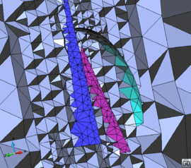
|
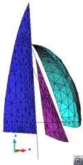
|
| (a) | (b) |
| Figure 104: Results for the validation example . (a) View of some internal tetrahedra with conformal to the triangle mesh of the sails. (b) Triangle and linear meshes of the model. | |
The data of the generated mesh of this validation example is detailed in Table 16.
| Number of threads | |
| Mesh general size (uol) | |
| Transition factor | |
| Number of tetrahedra | |
| Number of nodes | |
| Minimum dihedral angle (degrees) | |
| Time to generate the mesh (seconds) | |
| Speed (Mtetrahedra per minute) |
7.1.6 Embedded mesh
In this section, a validation example of an embedded mesh is presented. As explained in previous sections, an embedded mesh is not body fitted, so its generation is much more faster.
7.1.6.1 Validation example VE-E1
Validation example is a representative volume element (RVE) of a synthetic porous material. A view of the model is depicted in Figure 105.
|
|
| (a) | (b) |
| Figure 105: Model used in the validation example . (a) View of the geometry of the model with transparencies in its external surfaces in order to appreciate the internal voids of it. (b) View of the input mesh used for the mesher. | |
The model is a watertight volume with spherical voids (holes) representing the porous. The voids are made with randomly placed spheres of different diameters. The side of the cube is uol, and the diameters of the spheres goes from to uol. The minimum distance between the spheres and the boundaries of the cube (or between different spheres) is around uol. In order to capture better the interfaces between the voids and the material, a size of uol has been assigned to the input boundaries, and a general mesh size of uol has been assigned to the hole model. The is equal to 1.
The triangle mesh used as the input boundaries for the mesher is shown in Figure 105(b). It can be appreciated that the spherical voids are represented with a fine mesh in order to capture well their shape, as the external surfaces of the cube are represented only by two triangles each one of them. As they are planar, its shape is perfectly captured in this way.
|
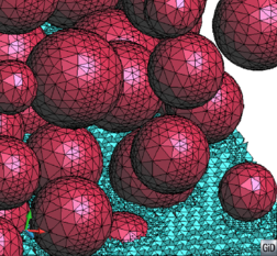
|
| (a) | (b) |
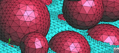
| |
| (c) Results for the validation example . (a) View of the inner part of the final tetrahedra mesh. (b) and (c) Details of the inner part of the final tetrahedra mesh together with the triangle mesh used as the input boundaries. | |
| Figure 106 | |
A view of the inner part of the generated mesh is shown in Figure 106. As it is a non body-fitted mesh, all the tetrahedra come directly from the tetrahedra pattern applied to the octree cells, with no distortion. The level of refinement near the input boundaries due to the smaller desired size applied onto it can be appreciated. In Figure 106(b) a detail of the mesh is depicted together with the input mesh for the mesher. It can be seen that the tetrahedra does not fit with the input boundaries.
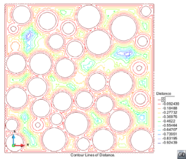
|
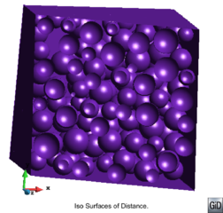
|
| (a) | (b) |
| Figure 107: Results for the validation example . (a) View of a cut of the model with the isolines of distance. (b) View of the iso-surface of distance in the inner part of the volume. | |
A view of the isolines of distance within a cut of the tetrahedra mesh is shown in Figure 107(a), and an inner view of the iso-surface of distance equal to is shown in Figure 107(b). It can be appreciated that the distances on the nodes are well computed.
The data of the generated mesh is detailed in Table 17.
| Number of threads | |
| Mesh general size (uol) | |
| Mesh size in input boundaries (uol) | |
| Transition factor | |
| Number of tetrahedra | |
| Number of nodes | |
| Time to generate the mesh (seconds) | |
| Speed (Mtetrahedra per minute) |
7.1.7 Performance
The validation examples in this section aim to evaluating the efficiency inofhe implementation of the algorithm. For this purpose several meshes of the same models are generated with different sizes in order to get an idea of the performance of the mesher.
It has to be considered that each model has its own particularities, making difficult to extrapolate the speed of the mesher from a model to another. However, knowing the characteristics of the model can give us an idea of the behavior of the mesher for other ones.
As some parts of the algorithm have been implemented using shared memory parallelism, the examples in this section are run with different number of threads (from to ) in order to evaluate its scalability.
For sake of the performance analysis, the following main parts of the algorithm are distinguished:
- Refinement. This relates to all the octree refinement processes and the operations they involve. In case of topology refinement criteria, for instance, the subdivision of a cell implies the creation of the linear octree nodes of its children, as well as their coloring and the determination of their closest point in boundary in case they come from an interface cell.
- Nodes and tetrahedra generation. This includes three main parts:
- The creation of the linear octree nodes just before the coloring process. In this step almost all the octree nodes are created, except the ones created during the topology refinement criteria. The creation of an octree node implies:
- The creation and storage of the node itself.
- The assignation of the corresponding octree position in the cells surrounding the node.
- The search and assignment of its closest position onto the input boundaries. This is done only to the nodes belonging to an interface cell.
- Creation of the tetrahedra from the interface cells applying the tetrahedra pattern. Within the creation of these tetrahedra, the information of the tetrahedra surrounding each node is also stored.
- Creation of tetrahedra from the inner cells following the tetrahedra pattern. These tetrahedra are created at the end of the meshing process, as they are directly part of the final mesh (no mesh edition is performed on them). In this case no neighboring information is stored in the nodes.
- Coloring. This part corresponds to the node coloring process, following the ray casting technique (Section 4). It has to be considered that the majority of the nodes are colored in this step, but not all of them. The coloring of the octree nodes created during the topology refinement criteria is performed inside the refinement part.
- Surface fitting. This part corresponds exactly to the surface fitting process defined in Section 5.3.6.
- Tetrahedra coloring. All the tetrahedra coloring operations, as well as the creation of skin triangles of tetrahedra of the same color, are included in this part. It has to be noted that the process of coloring an undetermined tetrahedra may involve the coloring of some positions in space (points onto some tetrahedra face).
- Make-up and smoothing. This part consists in the following processes:
- Collapse of small edges performed just after the surface fitting process.
- Tetrahedra swapping.
- Smoothing process involving movement of nodes.
- Others. All the other processes of the meshing algorithm not present in the previous ones are included in this part. It is the case, for instance, of the operations related to the preservation of geometric features. It is not treated apart because it is really low time consuming.
7.1.7.1 Validation example VE-S1
The most favorable case for the presented mesher is a model as much massive as possible (maximum sphericity), watertight, with no geometrical features to be preserved, and with a uniform mesh size. The validation example is a sphere of uol of diameter, which fits with these characteristics. The results of this validation test case should provide with an upper limit for assessing the performance of the mesher.
Four different configurations of the sphere have been run, corresponding to different uniform mesh sizes. Each one of the configurations has used a triangle mesh of the same size as the one of the volume as the input boundary.
The minimum dihedral angle of the tetrahedra generated is higher than degrees in all the configurations.
All the configurations have been run using , , and threads. The results of speed and speed-up for each configuration are depicted in Figure 108.
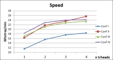
|
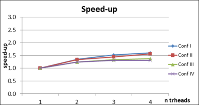
|
| (a) | (b) |
| Figure 108: Graphs of (a) speed (in Mtetrahedra per minute) and speed-up (b) corresponding to the four configurations of validation example . | |
The characteristics of each configuration are depicted in Table 18.
| Configuration | I | II | III | IV |
| Mesh size | ||||
| Number of tetrahedra (millions) | ||||
| Number of nodes (millions) | ||||
| Memory peak (Gb) | ||||
| Memory ratio |
As it can be appreciated, in this example the mesher generates between and millions of tetrahedra per minute (using one thread), depending on the configuration. Increasing the number of threads results in a low speed-up, arriving at around when threads are used. The speed-up is far from the optimal one because of the implementation of the algorithm. The current implementation has been focused in parallelizing the naturally parallel parts of the algorithm. The other parts could be also implemented in parallel, reaching higher speed-up values.
The distribution of time consumed by the main parts of the mesher changes depending on the configuration. The reason for this is the node and tetrahedra generation part is basically proportional to the number of tetrahedra and nodes to be created. This is not the case of the other parts of the algorithm, as they are mostly applied only to the tetrahedra near the contours of the volume.
The distribution of computing times corresponding to configuration IV for the different number of threads used is depicted in Figure 109.
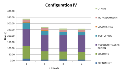
|
| Figure 109: Time consumed in the meshing process of configuration IV of validation example detailed in the different parts of the algorithm. |
It has to be noted that this example (a uniform meshed sphere) is quite particular as some of the main parts of the presented mesher are not representative. The tetrahedra coloring algorithm, for instance, is not applied in this case as there are no undetermined tetrahedra after the surface fitting process. Furthermore this is the model with maximum possible sphericity, so the majority of the tetrahedra (the inner ones) comes directly from applying of the tetrahedra patterns.
7.1.7.2 Validation example VE-S2
This validation example is a synthetic model of a city. A view of the model is depicted in Figure 110.
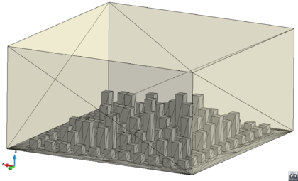
|
| Figure 110: Model used in the validation example . |
The model basically consists in prismatic shapes representing buildings, connected to a planar terrain, and enclosed in a unique watertight control volume. The base of the control volume is by uol, and its height is uol. All the buildings have a base of by uol (they are also separated this distance one from eachother) and their heights go from to uol. A zoom view of some of the buildings is shown in Figure 111.
This model is not so favorable for the mesher, as it contains sharp edges to be preserved, and it will not be meshed with a uniform size, so it could give a more realistic idea of the performance of the mesher applied to real models. The sphericity of the model is .
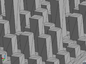
|
| Figure 111: Zoom of the buildings of the model used in the validation example . |
In this case also four configurations have been used to check the performance and scalability of the mesher. Each configuration has the same input boundary (shown in Figure 110(a)), made by triangles. A of is used, and two sizes are assigned: one for the surface entities defining the terrain and the buildings, and a general mesh size for the rest of the domain.
The characteristics of each configuration are detailed in Table 19. The minimum dihedral angle of the tetrahedra generated is higher than degrees in all the configurations.
| Configuration | I | II | III | IV |
| Mesh size in buildings | ||||
| Mesh general size | ||||
| Number of tetrahedra (millions) | ||||
| Number of nodes (millions) | ||||
| Memory peak (Gb) | ||||
| Memory ratio |
All the configurations have been run using , , and threads. The results of speed and speed-up for each configuration are depicted in Figure 112.
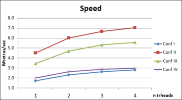
|
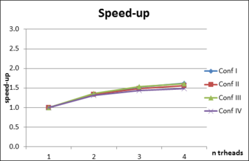
|
| (a) | (b) |
| Figure 112: Graphs of (a) speed (in Mtetrahedra per minute) and speed-up (b) corresponding to the four configurations of validation example . | |
The results obtained in this example show that the mesher generates between and millions of tetrahedra per minute (using thread), depending on the configuration. The speed-up reaches using threads.
The distribution of computing time in the different parts of the mesher is rather similar in the 4 configurations. The one corresponding to configuration IV using thread is depicted in Figure 113. It can be seen that the most consuming parts of the algorithm in this example are the refinement, the mesh improvement operations (make-up and smoothing) and the surface fitting process. Considering the refinement part, more than the half of the time is devoted to the topology refinement criteria.
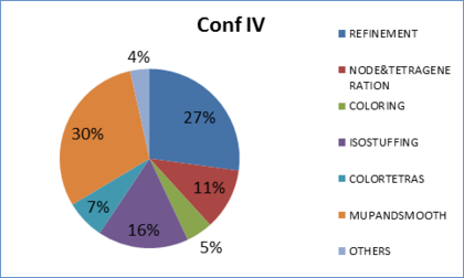
|
| Figure 113: Percentages of time consumed in the meshing process of configuration IV of validation example . |
The speed-up curves of the most relevant parts of the algorithm are depicted in Figure 114. As it can be appreciated, none of them presents an optimal speed-up. This is the reason of the low speed-up reached considering the whole meshing process. The surface fitting process is the one with a higher speed-up, reaching almost with threads.
Some aspects of the implementation of the algorithm could be improved in order to reach a higher speed-up for the whole meshing process.
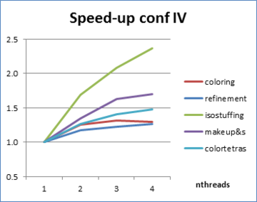
|
| Figure 114: Speed-up of the main parts of the algorithm generating the mesh of validation example . |
7.2 Racing car example
The model used in this section corresponds to a racing car. Specifically, the part of interest for a CFD numerical simulation is the air surrounding the car. For this reason a synthetic wind tunnel (a control volume) has to be build around it. For a CFD simulation the control volume must be large enough to avoid any influence of the boundary conditions in the results. In this example only a small control volume has been build, considering the more interesting part from the meshing point of view is the region near its surfaces.
To run a CFD simulation on this model would imply also to generate a boundary layer mesh near the surfaces of the car and the floor. This is a specific kind of mesh with very thin elements in the normal direction of the flow in order to capture well the high velocity gradients present in that regions.
The generation of the boundary layer mesh is out of the scope of this work, but its requirements have been taken into account. There are two main families of boundary layer meshes:
- A priori: this approach generates first a boundary layer mesh from the input surface entities towards the inner part of the volume. After a given number of layers of elements, the contours of this mesh are used as the input boundaries to feed an isotropic volume mesher [DBLP:conf/imr/GarimellaS98,romainlohner].
- A posteriori: in this case the isotropic mesh is generated first, and afterwards the boundary layer elements are generated from the contours of the isotropic mesh pushing towards the interior of the volume the existing tetrahedra [65]. As it implies the movement of nodes, typically a re-positioning of the nodes near the boundary layer mesh is needed.
As the presented mesher is not constrained (the volume mesh is not conformal to the input surface entities), a boundary layer mesh cannot be generated a priori, so a posteriori method should be used. In the presented example the boundary layer mesh has not been generated, as it is considered as a separated process, and is out of the scope of the monography.
The model is watertight. Some figures of the geometry of the model with its characteristic sizes are shown in Figure 115. Views of the input surface mesh used are depicted in Figure 116. It can be appreciated that the quality of the input surface mesh is quite good, so it could be used probably as an input for an advancing front based mesher. For generating the volume mesh of this model using the presented octree mesher a worse quality mesh could be used to define the boundaries, saving the corresponding time on the surface meshing part.
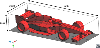
|
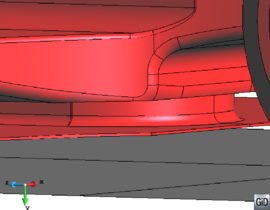
|
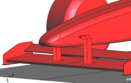
|
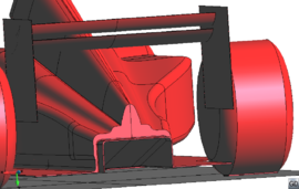
|
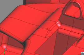
| |
| Figure 115: Different views of the racing car model to be meshed of in this section. | |
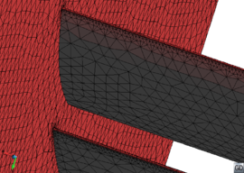
|
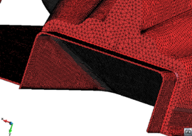
|
| Figure 116: Different views of the triangle mesh used as input boundaries for the racing car model. | |
The mesh has been generated setting a mesh size of uol in the skin of the car, as well as the floor, and a uol in the outlet of the control volume (the surface enclosing the control volume in the rear part of the car). No general mesh size has been assigned, so the element size should grow with the distance to the car and the outlet surface accordingly to the size transition function. A of has been used.
The data of the generated mesh of this example is detailed in Table 20.
| Mesh general size (uol) | None |
| Mesh size in skin of the car and floor (uol) | |
| Mesh size in outlet surface (uol) | |
| Transition factor | |
| Number of tetrahedra (millions) | |
| Number of nodes (millions) | |
| Minimum dihedral angle (degrees) | |
| Number of elements with t min dihedral angle |
Some views of the tetrahedra mesh generated are depicted in Figure 118. It can be appreciated the effect of the size transition function. As the used in this model is lower than , the size of the elements is not growing until a given distance to the skin of the car. However, the octree configuration where the tetrahedra come from force to double the size of the elements at this point, so the size transition is not as gradual as in other meshing methods (like advancing front based ones). A equal to would lead to a faster transition governed by the 2 to 1 constraint. zoom views or the skin mesh of the tetrahedra generated is shown in Figure 117.
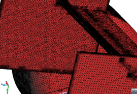
|
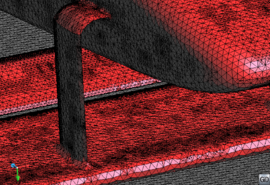
|
| Figure 117: Different views of the skin mesh of the tetrahedra generated for the racing car model. | |
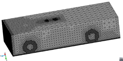
|
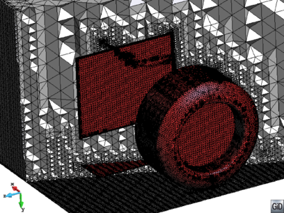
|
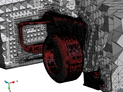
| |
| Figure 118: Different views of the final tetrahedral mesh for the racing car model. | |
The mesh has been generated using , , and threads. The results of speed and speed-up for each configuration are depicted in Figure 119. As it can be seen, the maximum speed-up reached is using threads.
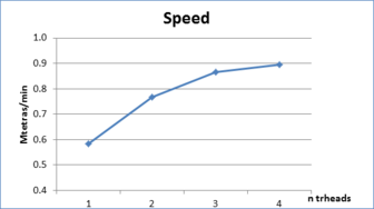
|
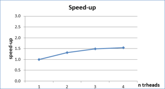
|
| (a) | (b) |
| Figure 119: Graphs of (a) speed (in Mtetrahedra per minute) and speed-up (b) corresponding to the racing car example. | |
The distribution of CPU time in the different parts of the algorithm using thread is depicted in Figure 120. It can be appreciated that in this example the refinement part takes more relevance than in the other examples. Specifically, the octree refinement considering the input mesh sizes and their propagation using the size transition function takes around of the refinement time. This is due to the distribution of mesh size entities used in this model: all the triangles from the input mesh of the skin surfaces of the car and the floor are mesh size entities corresponding to uol. Each one of this triangle generates the corresponding generalized mesh size points, from which the size transition function is applied to propagate the minimum and maximum sizes allowed to the surrounding octree cells considering the influence radius.
The tetrahedra coloring part also consumes an important part of the meshing process in this example. Because of the nature of the model (there are very thin parts to be meshed), there are many tetrahedra with all their nodes in the interface (undetermined tetrahedra) that must be colored using the methodology explained in section 5.3.7.
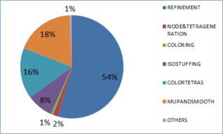
|
| Figure 120: Percentages of CPU time consumed in the meshing process for the racing car example. |
7.3 Barcelona city model
In this example a model of the city of Barcelona is used to generate an embedded mesh. Actually, the model used is a part of the model of the whole city. The model has been provided by the Virtual Visualization Lab, from Barcelona Media company [66], and consists in the Digital Terrain Model (DTM) and simplified models of the buildings.
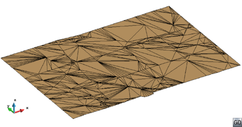
|
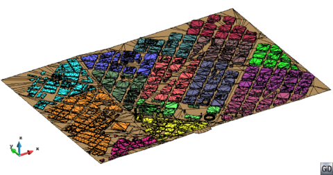
|
| (a) | (b) |
| Figure 121: Model of a part of the city of Barcelona used in this example. (a) View of the digital terrain model (DTM). (b) View of the DTM and the buildings. | |
The scale of the model is and there is no topological connection between the buildings and the terrain model. A view of the DTM and the buildings can be appreciated in Figure 121.
Some zoom views of the model are depicted in Figure 122. As it can be seen, the level of definition of the buildings does not capture all their details, but it is accurate enough to perform a CFD simulation of the air flow around them in the urban environment. It can also be appreciated that the buildings models are not represented by a watertight definition, as they have not any surface entity in its lower part. Furthermore, some of them have gaps and overlapping entities.
|
|
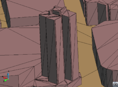
|
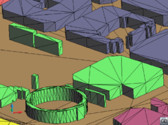
|
| Figure 122: Zoom view of some part of the Barcelona city model in order to appreciate the level of detail of the buildings description. In the first figure it can be appreciated that the building models are opened in their lower part. | |
The presented model is basically a collection of surface entities defining the skin of the city which must act as a barrier for the air flow in an aerodynamic simulation. In order to generate the tetrahedra mesh of the air surrounding the buildings, a volume must be created. Furthermore, as an embedded mesh will be generated, another volume must be created to indicate whether a node is inside the air domain or not. For notation purposes, let us distinguish between the control volume and the embedded volume:
- The control volume is the one where the tetrahedra for the simulation will be generated.
- The embedded volume gives the topological information needed to indicate if a node is inside or outside the fluid domain (where the air flow is calculated). From the topological point of view, the embedded volume can be considered as a hole in the control volume where the simulation should not be applied.
A view of the embedded volume is depicted in Figure 123(a), and the control volume is shown in Figure 123(b). The control volume is extremely simple; it is just a parallepiped. Its shape has been chosen taken into account the way of assigning the boundary conditions of a numerical simulation. The control volume may overlap partially or completely the embedded volume. However, this overlapping does not require a topological relationship between both volumes, which simplifies much its definition.
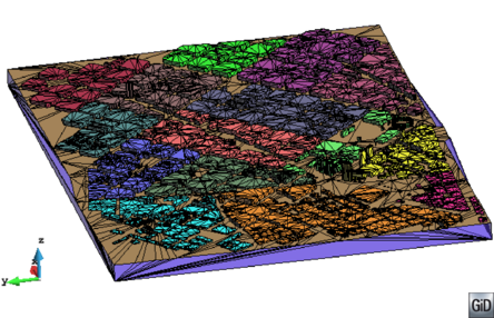
|
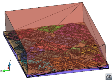
|
| (a) | (b) |
| Figure 123: Barcelona city model. Volumes defined to generate the embedded mesh. (a) Volume defining the lower part of the city, which will act as a hole of the control volume. (b) Control volume where the mesh will be generated. | |
The embedded volume is a non-watertight volume, as the DTM and the buildings have gaps and overlapping entities. Some view of the higher entities of the edges of the DTM and the buildings are shown in Figure 124. Recall that all the edges should have a higher entity value equal to 2 in a watertight volume.
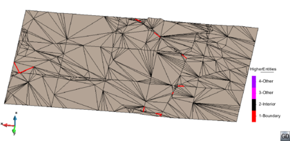
|
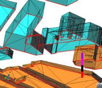
|
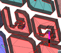
| |
| Figure 124: Different views of the higher entities of the edges of the DTM (upper figure) and some of the buildings (two figures at the bottom). Red edges are considered as boundaries, as they have higher entity equal to . | |
More than non-watertight, this volume is not correctly defined due to the way the buildings are presented with respect to the DTM. 2D schematic embedded surfaces trying to represent this situation are depicted in Figure 125. A scheme of a watertight embedded surface including only the terrain is depicted in Figure 125(a). A watertight definition of the embedded surface including a building is shown in Figure 125(b). A possible valid non-watertight definition of the embedded surface could be the one depicted in Figure 125(c), where there is no topological contact between the terrain and the building. Here, the size of the gap and the overlapping entities in the contact region must be small enough to be used in the coloring process.
The configuration given for this example corresponds to the scheme shown in Figure 125(d). In this case, the part of the embedded volume inside the building is not well defined, as there is a boundary entity (segment in Figure 125(d)) which definition indicates is interfacing the volume and its outer part, but in reality, this boundary is totally inner to the volume. This situation may set as invalid some of the rays aligned with Z direction used in the coloring process.

|
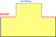
|
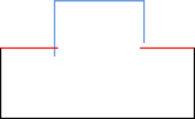
|
| (a) | (b) | (c) |
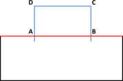
| ||
| (d) | ||
| Figure 125: Barcelona city model. 2D schemes illustrating the bad definition of the embedded volume. (a) Scheme of embedded surface only including the terrain (in red). (b) Scheme of a watertight embedded surface including the terrain and a building (in blue). (c) Scheme of a valid non-watertight definition of the embedded surface. (d) Scheme of a bad definition of the embedded surface including the terrain and a building. | ||
The meshing process of this example is based in two main steps:
- Body fitted mesh. A body fitted mesh of the control volume is generated taking into account the input mesh sizes and not considering the boundaries of the embedded volume.
- Embedded coloring. The nodes of the generated body fitted mesh are colored and their distances to the boundaries are calculated, considering only the surface entities contour of the embedded volume.
Although the meshing algorithm accepts non-watertight geometries as an input, some cleaning operations have been made to the original model, in order to be able to generate the mesh:
- First of all, a rectangular shaped portion of the whole city model have been selected, and the rest part of it have been deleted.
- Delete some internal surface entities present in the buildings. This internal surfaces may affect negatively the node coloring process.
This CAD cleaning operations are considerably simpler and less time consumer than the required to make the model watertight. The time needed to perform these operations manually is less than one hour.
The bad definition of this model make totally necessary the local ray casting operations applied to the nodes where the three Cartesian rays are invalid. Actually, the Cartesian rays color most of the nodes of the model, setting as uncolored the ones in the bad definitions of the boundaries. In these ones the local ray casting is performed.
An adaptation of the local ray casting process has been made in order to deal with this bad defined model. The model has gaps, nevertheless, the pathological situation of this model is given by a sort of fake interface entity (the segment in Figure 125(d)). This should lead to erroneous colors provided by some local ray, like the ones depicted in Figure 126. In that figure, node should be colored using local rays from its three surrounding nodes: , and . Node is outside the volume, and the other two are inside. The ray from node determines that is inner to the volume, as it intersects one time the interface (between inner and outer parts), and node is an outer node. The ray from node also set as inner node, as it has no intersections and node is also an inner node. The problem comes from the ray from node : it has one intersection and is inner to the volume, so it should consider as outer node, which is an error.
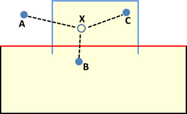
|
| Figure 126: Scheme of local rays used to color node in a bad defined model. Local rays from nodes and set node as an inner node. Local ray from node provides with bad information, as set the node as outer. |
The voting process among the local rays used to color a node may take a bad decision depending on the configuration of the neighbors of the node. The adaptation to the local ray casting technique implemented in order to solve this situation is to give priority to the local rays with no intersection. If there are local rays with no intersections, their information is used, otherwise the ones with intersections are considered.
The mesh has been generated with a desired mesh size of uol for the buildings surface entities, uol for the terrain and leaving the mesher to increase the size in the volume accordingly to a transition factor of . The data of the generated mesh is detailed in Table 21.
| Mesh general size (uol) | None |
| Mesh size in buildings (uol) | |
| Mesh size in terrain (uol) | |
| Transition factor | |
| Number of tetrahedra (millions) | |
| Number of nodes (millions) | |
| Minimum dihedral angle (degrees) |
A zoom view of the inner tetrahedra of the final mesh together with the input boundaries is depicted in Figure 127.
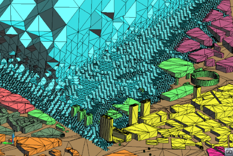
|
| Figure 127: Final mesh for the Barcelona city model. Zoom view of the inner part of the mesh together with the input boundaries. |
A view of the exterior part of the generated mesh is shown in Figure 128(a), and a view of the contourfill of computed distances for embedded method in a cut of the mesh is shown in Figure 128(b), together with the isosurface of distance equal to zero extracted from the generated mesh. Two zoom views of this isosurface are depicted in Figure 129.
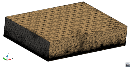
|
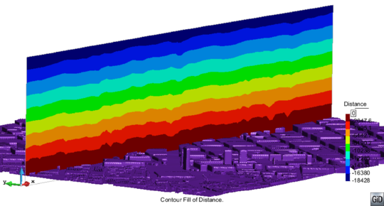
|
| (a) | (b) |
| Figure 128: Final mesh for the Barcelona city model. (a) View of the external part of the mesh. (b) View of the contourfill of distances in a cut plane made on the generated mesh, together with the isosurface corresponding to distance zero. | |
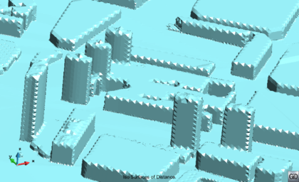
|
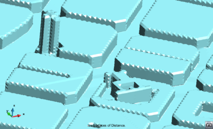
|
| Figure 129: Zoom views of the isosurface corresponding to a distance of the mesh generated in Barcelona model. | |
It can be appreciated that the isosurface corresponding to distance zero is not capturing well the sharp edges of the domain. In this work the coloring of the nodes and the distance propagation is done at global level, only considering the nodes. In order to improve the algorithm the distance of the nodes could be treated locally, considering the edges of the mesh and their intersection points with the input boundaries. Depending on the requirements of the simulation to be done it may be important or not to preserve these geometrical features.
The mesh has been generated using , , and threads. The results of speed for each configuration are depicted in Figure 130. As it can be seen, Mtetrahedra per minute are generated in serial. The maximum speed-up reached is using threads, and the memory peak during the meshing process is Gb.
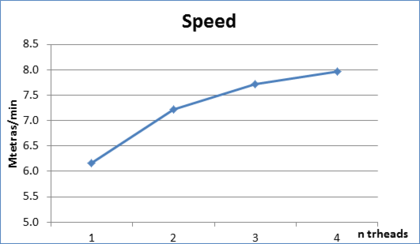
|
| Figure 130: Graph of speed (in Mtetrahedra per minute) corresponding to the Barcelona model example. |
The distribution of times devoted to the two main parts of the algorithm (body fitted mesh of the control volume and embedded coloring) is depicted in Figure 131. It has to be considered that the embedded coloring part includes:
- Enter the surface entities of the embedded volume into the octree. This automatically sets the interface cells.
- Compute the exact distance to the boundaries of the nodes belonging to the interface cells.
- Perform the coloring and compute of distances to the nodes using the ray casting technique.
It can be appreciated that (in serial), both parts of the meshing process consumes approximately the same time.
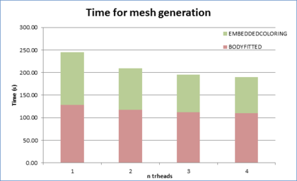
|
| Figure 131: Times consumed for the meshing of the Barcelona model example detailed in the two main parts of the algorithm. |
7.4 General overview
A general analysis of the body-fitted mesher is done in this section. It is based on the results of the examples with more than one million tetrahedra, which are the following ones:
- Validation example .
- Validation example (the four configurations).
- Validation example (the four configurations).
- Racing car example.
The smaller examples are not considered in this section because they should be affected by the time measurements.
Concerning the embedded mesher, as few cases have been run, its analysis is done in the sections of the corresponding examples.
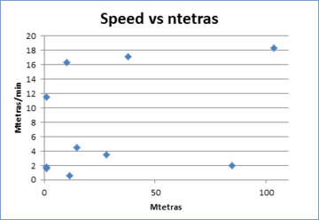
|
| Figure 132: Graph relating the speed of generation (Mtetrahedra per minute) and the number of tetrahedra generated. |
The speed of the mesher is quite variable depending on the characteristics of the model, going from to millions of tetrahedra per minute. Having a look at Figure 132, no relationship between the speed of the mesher and the number of tetrahedra generated can be established. This was expected, as in the presented mesher the main part of the effort is put in the tetrahedra near the boundary, while the inner ones are created very fast.
For this reason, in order to evaluate and compare the speed of an octree based mesher is more appropriate to consider the sphericity of the model to be meshed. A graph relating the speed and the sphericity is shown in Figure 133(a).
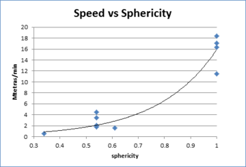
|
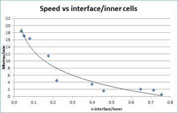
|
| (a) | (b) |
| Figure 133: Speed of tetrahedra generation (Mtetrahedra per minute) versus (a) shpericity of the model and (b) ratio between number of interface and inner cells. Logarithmic tendency line in black. | |
It can be seen that the mesher is faster as the model to be meshed is more massive (higher sphericity), independently on the number of tetrahedra generated. However, it can be appreciated that the same model (with the same sphericity) presents different speeds depending on the configuration of the example. The reason for this is that present implementation of the mesher dedicates almost all the effort in the treatment of the tetrahedra coming from the interface cells, so the same model with different sizes assigned to it may have different ratio between the tetrahedra near the interface and the inner ones.
In order to normalize the speed of the mesher considering this effect, a graph relating the speed of the mesher with the ratio between interface and inner cells is depicted in Figure 133(b). The behaviour of the mesher is well captured, and the speed increases as the ratio decreases.
Considering the main parts of the algorithm defined in Section 7.1.7 for performance analysis, the percentages of time for each one of these parts are very different in the examples. Depending on the characteristics of the geometrical model and the input parameters, it may be more relevant the octree refinement, the surface fitting process, the tetrahedra coloring or the mesh improvement operations (make-up and smoothing). However, the nodes coloring process is rather fast in all the examples.
It has to be commented that this work has been more focused on the mesh generation than on its improvement, so it is expected that the implementation of make-up and smoothing operations can be improved, and this will affect the percentages of time of the different parts of the algorithm.
Concerning the memory consumed by the mesher, all the examples run have a ratio between the memory peak and the memory needed to store the mesh lower than , which represents approximately Gb per Mtetrahedra. A graph of the memory peak value for the examples analyzed is depicted in Figure 134. It can be appreciated that the memory peak needed to generate a mesh with the presented mesher is rather linear with the number of tetrahedra generated.
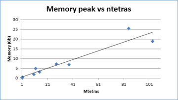
|
| Figure 134: Peak memory consumed (Gb) during the meshing process. Linear tendency line in black. |
The examples studied show that the implementation done has a low scalability when running in parallel. Values of speed-up have been reached using threads, which are far from the optimal ones (4). It has to be commented that this work has been more focused on the algorithm rather than on its implementation: more effort has been put in order to guarantee the mesh is generated than in the parallel implementation of the method. For this reason, it is expected that improvements in the implementation of the algorithm could reach a higher speed-up value. Nevertheless, the implementation of an algorithm always involves a trade-off between the speed and the memory allocated, so an improvement in speed may lead to an increase of memory allocated.
Furthermore the algorithm is based in non-consecutive usage of the memory. Although it has not been measured, a decrease in the cache use efficiency, specially in parallel computations, is expected.
7.4.1 Comparison with other methods
The considerations explained above with regards to the speed of the mesher make it difficult to compare the new mesher with other methods.
Some representative values are presented in Table 22 in order to have an order of magnitude. The method is compared with the advancing front based mesher present in GiD [56,57,58] and the Delaunay based mesher implemented in Tetgen [61], running in the same computer used in the present work.
| Octree-based mesher (this work) | to |
| Advancing front (GiD) | to |
| Delaunay (Tetgen) | to |
It has to be also considered that the implementation of a mesher can affect drastically its performance, so the values provided should be used only as an order of magnitude. There are implementations of advancing front meshers, for instance, reaching a speed of million of tetrahedra per minute [11] using a similar computer than the used in this work.
Another difficulty at the time of comparing speed of different mesher is the mesh improvement operations (make-up and smoothing) performed after the mesh generation itself. The effort needed for this operations depends strongly on two aspects:
- The quality of the mesh just before the mesh generation.
- The quality required by the simulation to be run using that mesh.
These two aspects are not typically specified, so the speed comparison between methods has to be analyzed carefully.
One consideration to be done when comparing the presented mesher with an advancing front-based one is the requirements they have (in terms of quality) on the input boundaries defining the domain. The new octree-based mesher accepts very bad shaped triangles as input boundaries, returning a good quality triangle mesh as the contours of the tetrahedra generated. Advancing front methods require a very good quality contours mesh, so before the volume mesh generation an extra effort should be added in order to edit (or even to regenerate) the contour mesh. In some cases the CAD cleaning operations to reach the final mesh are more time consuming than the mesh generation itself.
No other octree-based mesher has been used in the present work in order to compare the performance. Most of the octree meshers are based on hexahedral meshing, and not all of them satisfy the main requirements presented in this work (basically geometrical features and topology preservation). However, to have an order or magnitude, speeds between and Mtetrahedra per second can be found in the literature [37,40] considering octree-based meshers with the same characteristics as the developed in this work. It has to be considered that the computer used is different for this cases: [37] used a Mac Pro with 2.66 GHz Intel Xeon processor, and [40] a GHz octo-core mac xserve.
Concerning the memory consumed during the meshing process, the presented method consumes approximately the half of the advancing front and Delaunay implementations compared.
8 Conclusions and future lines
8.1 Conclusions
A robust and fast tetrahedra octree based mesher has been developed for embedded and body fitted meshes considering the requirements defined in Section 1.2. An innovative algorithm has been proposed to preserve the geometrical features and the topology of the domain accepting non-watertight definitions of the model. To reach these objectives some improvements and adaptations have been done in existing techniques (such as the ray casting method) in order to solve the Point In Polygon problem considering several volumes.
The effectiveness of the algorithm and its implementation has been verified in some validation examples. The mesh generator preserves the geometrical features and the topology of the model. Examples of non-watertight definitions of the domain have been meshed successfully thanks to the coloring algorithm designed based on the ray casting technique.
A summary of key features of the presented work is listed hereafter:
- The body-fitted mesher preserves the geometrical features existing in the domain, such as ridges and corners.
- The topology of the volumes defining the domain is preserved by the body-fitted meshing algorithm.
- The mesher can generate tetrahedra meshes from non-watertight definitions of the volumes. Cases with gaps and overlapping entities in the definition of their boundaries have been meshed successfully.
- The mesher has been adapted to generate embedded and body-fitted meshes.
- The examples run indicate that the mesher is very robust considering different input parameters. Even when no input parameters are introduced, it generates a valid mesh of the domain.
- The mesher is very robust considering the quality of the input mesh. An important advantage of the mesher is that the triangle mesh defining the boundaries is not needed to have good shaped elements. The only requirement for the input mesh is to represent precisely the shape of the contours, which only implies the fulfillment of a given chordal error criterion. For this purpose typical surface render meshes (optimized for visualization purposes) can be used. As these meshes are often provided by the CAD systems, most CAD cleaning operations are saved using this mesher, with the corresponding saving in time. However, if the quality of the input mesh is very low, some pre-treatment may be done in order to detect the sharp edges to be preserved by the mesher. This part is considered external to the mesher.
- The new mesher is independent of the size of the input boundaries. This makes possible to use the same definition of the domain to generate different volume meshes.
- A strategy has been proposed for embedded meshes combining the body fitted mesher for the control volume, and the node coloring and distances propagation considering the contours of the embedded volume.
- The results from the examples studied show that the mesher is fast in comparison with other meshers analyzed. Depending on the characteristics of the model, the mesher generates between and millions of tetrahedra per minute on a desktop PC.
- A robust and efficient point coloring algorithm based on a ray casting technique have been designed and implemented in order to detect where the nodes of the mesh are: inside a given volume or laying on an interface between volumes. This coloring algorithm works in domains with several volumes and works with non-watertight definitions of them. A solution has been proposed for solving the pathological cases for ray casting technique. The coloring algorithm has been adapted to compute the distances of the nodes of the mesh to the input boundaries for embedded meshes, using the Manhattan distance as an approximation of the exact one.
- An algorithm has been proposed to color the tetrahedra with all its nodes in interface entities: that is, determine the volume these tetrahedra belongs to. This algorithm ensures the preservation of the topology of the model.
- The mesher generates jointly the meshes of several volumes if they share some line or surface entity, and gets as input data triangle meshes defining the boundaries of the volumes.
- The mesh resulting from the meshing algorithm may have poor quality elements depending on the characteristics of the model. For this reason make-up and smoothing operations have been implemented in order to improve the quality of the mesh.
- The presented mesher tries to fit the final mesh with the desired mesh size, but this cannot always be accomplished precisely. This is because the tetrahedra generated come directly from the octree cells, and their size comes from subdividing the octree root recursively. Size transitions between regions with different desired size are controlled by a size transition function. However, the final mesh cannot reproduce smooth size transitions, as the octree cells sizes changes by a factor of two in each refining process.
- The octree structure has been adapted successfully to the mesh generation, using an efficient implementation of a binary octree.
- The current implementation does not preserve the topology of the model in configurations where no proper input mesh size is provided and consequently, if the domain presents very thin parts in comparison with its characteristic length, the topology may not be preserved.
- The isotropic structure of the octree may lead to excessive refined tetrahedra meshes near the boundaries in comparison to other meshing methods.
- The algorithm has been adapted to generate 3D surface meshes which are inner to a volume, or isolated in space.
- The implementation of the mesher has been done following the OpenMP paradigm for parallelizing some of the parts of the algorithm. Nevertheless, the maximum speed-up reached is using threads, which is considered to be improvable.
- The implementation of the mesher generates meshes consuming less than times the memory needed to store the final mesh. This represents approximately Gb of peak memory per Mtetrahedra generated. This is less than the other meshing techniques analysed in this work.
- The mesher could be used for CAD cleaning operations, as it can return a watertight mesh from a non-watertight one.
The mesher has been implemented as a static library and it is used by the version 11.1.9d of the pre and post-processor GiD [63].
8.2 Future research lines
From the design and implementation of the meshing algorithm presented in this work, the following future research lines have been identified:
- Improve the implementation of the algorithm. This work has been focused more on the algorithm rather than on its parallel implementation. The serial part can be parallelized and the parallel part can be improved.
- Implement the meshing algorithm using distributed memory paradigm (MPI). This kind of implementations uses a decomposition of the space in order to treat independently separated parts of it. As the octree structure is a decomposition of the space itself, the implementation could take advantages of its characteristics. However, focusing in one part of the domain, some of the octree refinement criteria need information of other parts, so the implementation of the algorithm is not obvious.
- Improve the make-up and smoothing operations. These operations can be improved in order to get better quality meshes using less time. Furthermore, a coarsening operation could be added in order to avoid the excessive level of refinement present in some parts of the boundaries of the volumes.
- Adapt the mesher to work with 3D images as a definition of the input boundaries (such as medical images (IMR), or tomography ones). In these cases, the boundaries of the volumes involved in the domain are not defined explicitly: they can be extracted from a distance function applied to a 3D regular grid of points. As the presented mesher uses an octree (which a regular grid is an specific case), the information of the distances can be included directly in the algorithm and some of its processes can be adapted to generate the mesh of the different volumes of the domain.
- Adapt the algorithm to generate hexahedra meshes. Actually, the inner cells of the octree are already hexahedra, so they could be used as final elements, defining a given pattern for the cases where two neighbor cells are in different levels (have different size) in order to generate a conformal mesh. The more complicated parts of the algorithm to reach this goal should be the preservation of the geometrical features and the surface fitting process. In the present algorithm, these processes involve the splitting of tetrahedra edges or faces. These operations generate automatically new tetrahedra, but applying them to hexahedra should generate other types of polyhedral. This should require to define a sort of transition element types, or to redefine directly some of the operations involved.
- Adapt the mesher to NURBS curves and surfaces as input for defining the volumes boundaries and forced line entities. The smoother definition of NURBS compared with meshes ensures a better approximation to the shape of the domain. Theoretically the design of the algorithm has been done considering this option, but in practice, the use of geometrical data instead of mesh data as input may lead to some difficulties in terms of implementation. Specially the operations involving intersections. Intersecting an edge with a triangle has a limited number of possible cases, but intersecting it with a NURBS surface is much more complicated, and can present several pathological configurations.
- Implement automatic tools in order to filter and detect the geometrical features to be preserved from the analysis of the input data. When the input boundaries have low quality, the normal of some of the triangles cannot be computed properly, so some edges can be set to be preserved when they are not really sharp edges. Actually, this part can be considered as external to the meshing algorithm, but enables the mesher to be called directly from a CAD system, which may automatize as much as possible the operations to create the input data and saves time at user level.
- Adapt the algorithm to models with specific topology. As seen in the example of the Barcelona city model, adapting slightly the ray casting coloring algorithm, the mesher can deal with bad topological definition of the domain. This can be interesting at the time of trying to adapt the mesher to a set of cases which may be bad defined, but may present known pathological situations. This is the case of most DTM models, as well as in CAD geometries coming from other sources.
- Implement the parts of the topological refinement criteria concerning surface and volume parts. Their implementation should ensure the topological preservation even when there are very thin parts in the model and no mesh size is provided to the mesher.
- For the embedded mesher, the distance from the nodes to the input boundaries can be treated locally, considering each edge of the mesh. This should help to capture the sharp edges of the model by the isosurface of distance zero.
BIBLIOGRAPHY
[1] Zienkiewicz, O.C. and Taylor, R.L. and Zhu, J.Z. (2005) "The Finite Element Method: Its Basis and Fundamentals: Its Basis and Fundamentals". Elsevier Science
[2] Oñate, E. (2009) "Structural Analysis with the Finite Element Method. Linear Statics: Volume 1: Basis and Solids". Springer
[3] Calvo, Nestor and Idelsohn, Sergio R and Oñate, Eugenio. (2003) "The extended Delaunay tessellation", Volume 20. MCB UP Ltd. Engineering Computations 5/6 583–600
[4] Gerald Farin. (1997) "Curves and surfaces for computer-aided geometric design - a practical guide (4. ed.)". Academic Press I-XVII, 1-429
[5] Jonathan Richard Shewchuk. (2012) "Combinatorial Scientific Computing". Chapman and Hall CRC 259-285
[6] Lai, Ming-Chih and Peskin, Charles S. (2000) "An immersed boundary method with formal second-order accuracy and reduced numerical viscosity", Volume 160. Elsevier. Journal of Computational Physics 2 705–719
[7] Löhner, Rainald and Cebral, Juan R and Camelli, Fernando E and Appanaboyina, S and Baum, Joseph D and Mestreau, Eric L and Soto, Orlando A. (2008) "Adaptive embedded and immersed unstructured grid techniques", Volume 197. Elsevier. Computer Methods in Applied Mechanics and Engineering 25 2173–2197
[8] Cebral, Juan R. and Camelli, Fernando E. and Lohner, Rainald. (2002) "A feature-preserving volumetric technique to merge surface triangulations", Volume 55. John Wiley & Sons, Ltd. International Journal for Numerical Methods in Engineering 2 177–190
[9] Nooruddin, Fakir S. and Turk, Greg. (2003) "Simplification and repair of polygonal models using volumetric techniques", Volume 9. IEEE. Visualization and Computer Graphics, IEEE Transactions on 2 191–205
[10] George, P.L. (1991) "Automatic mesh generation: application to finite element methods". Wiley
[11] Löhner, Rainald. (2008) "Applied Computational Fluid Dynamics Techniques: An Introduction Based on Finite Element Methods". Wiley
[12] Frey, P.J. and George, P.L. (2000) "Mesh Generation: Application to Finite Elements". Hermes Science Publications
[13] Zienkiewicz, OC and Phillips, DV. (1971) "An automatic mesh generation scheme for plane and curved surfaces by ‘isoparametric’co-ordinates", Volume 3. Wiley Online Library. International Journal for Numerical Methods in Engineering 4 519–528
[14] Lo, S. H. (1985) "A new mesh generation scheme for arbitrary planar domains", Volume 21. John Wiley & Sons, Ltd. International Journal for Numerical Methods in Engineering 8 1403–1426
[15] Rainald Löhner and Paresh Parikh. (1988) "Generation of Three-Dimensional Unstructured Grids by the Advancing-Front Method", Volume 8. International Journal For Numerical Methods in Fluids 1135-1149
[16] J Peraire and M Vahdati and K Morgan and O.C Zienkiewicz. (1987) "Adaptive remeshing for compressible flow computations", Volume 72. Journal of Computational Physics 2 449 - 466
[17] Nguyen-Van-Phai. (1982) "Automatic mesh generation with tetrahedron elements", Volume 18. John Wiley & Sons, Ltd. International Journal for Numerical Methods in Engineering 2 273–289
[18] Owen, Steven J and Saigal, Sunil. (2000) "H-Morph: an indirect approach to advancing front hex meshing", Volume 49. Wiley Online Library. International Journal for Numerical Methods in Engineering 1-2 289–312
[19] Löhner, Rainald and Oñate, Eugenio. (1998) "An advancing front point generation technique", Volume 14. John Wiley & Sons, Ltd. Communications in Numerical Methods in Engineering 12 1097–1108
[20] Jin, H and Tanner, RI. (1993) "Generation of unstructured tetrahedral meshes by advancing front technique", Volume 36. Wiley Online Library. International Journal for Numerical Methods in Engineering 11 1805–1823
[21] Frykestig, Jan. (1994) "Advancing front mesh generation techniques with application to the finite element method". Chalmers University of Technology
[22] Löhner, Rainald. (1993) "Matching semi-structured and unstructured grids for Navier-Stokes calculations", Volume 3348. AIAA paper 1993
[23] Löhner, Rainald. (1996) "Extensions and improvements of the advancing front grid generation technique", Volume 12. Wiley Online Library. Communications in numerical methods in engineering 10 683–702
[24] Rainald Löhner and Juan R. Cebral. (1999) "Parallel Advancing Front Grid Generation". International Meshing Roundtable, Sandia National Labs 67–74
[25] Cheng, Siu-Wing and Dey, Tamal K. and Shewchuk, Jonathan. (2012) "Delaunay Mesh Generation". Chapman & Hall/CRC, 1st Edition
[26] George, Paul-Louis and Borouchaki, Houman. (1998) "Delaunay triangulation and meshing: application to finite elements". Hermes Paris
[27] George, Paul-Louis and Hecht, Frédéric and Saltel, Éric. (1990) "Fully automatic mesh generator for 3d domains of any shape", Volume 2. Elsevier. IMPACT of Computing in Science and Engineering 3 187–218
[28] Baker, Timothy J. (1987) "Three dimensional mesh generation by triangulation of arbitrary point sets", Volume 87. AIAA paper 1124
[29] Baker, Timothy J. (1989) "Developments and trends in three-dimensional mesh generation", Volume 5. Elsevier. Applied Numerical Mathematics 4 275–304
[30] Weatherill, Nigel P. (1992) "Delaunay triangulation in computational fluid dynamics", Volume 24. Elsevier. Computers & Mathematics with Applications 5 129–150
[31] Akkiraju, N and Edelsbrunner, H and Facello, M and Fu, P and Mücke, E and Varela, C. (1995) "Alpha shapes: definition and software". Proceedings of the 1st International Computational Geometry Software Workshop 63–66
[32] Kohout, Josef and Kolingerová, Ivana and Zára, Jirí. (2005) "Parallel Delaunay triangulation in E2 and E3 for computers with shared memory", Volume 31. Elsevier. Parallel Computing 5 491–522
[33] Blandford, Daniel K and Blelloch, Guy E and Kadow, Clemens. (2006) "Engineering a compact parallel Delaunay algorithm in 3D". ACM. Proceedings of the twenty-second annual symposium on Computational geometry 292–300
[34] Samet, H. (2006) "Foundations of Multidimensional and Metric Data Structures". Elsevier Science
[35] Yerry, M. A. and Shephard, M.S. (1984) "Automatic Three-Dimensional Mesh Generation by the Modified-Octree Technique", Volume 20. International Journal For Numerical Methods in Engineering 1965-1990
[36] Schneiders, R. (1996) "A grid-based algorithm for the generation of hexahedral element meshes", Volume 12. Springer-Verlag. Engineering with Computers 168-177
[37] Labelle, Francois and Shewchuk, Jonathan Richard. (2007) "Isosurface stuffing: fast tetrahedral meshes with good dihedral angles", Volume 26. ACM. ACM Trans. Graph. 3
[38] Mitchell, Scott A and Vavasis, Stephen A. (1992) "Quality mesh generation in three dimensions". ACM. Proceedings of the eighth annual symposium on Computational geometry 212–221
[39] Bern, Marshall and Eppstein, David and Gilbert, John. (1994) "Provably good mesh generation", Volume 48. Elsevier. Journal of Computer and System Sciences 3 384–409
[40] Maréchal, Loïc. (2009) "Advances in Octree-Based All-Hexahedral Mesh Generation: Handling Sharp Features". Proceedings of the 18th International Meshing Roundtable. Springer Berlin Heidelberg 65-84
[41] Shephard, Mark S. and Georges, Marcel K. (1991) "Automatic three-dimensional mesh generation by the finite octree technique", Volume 32. John Wiley & Sons, Ltd. International Journal for Numerical Methods in Engineering 4 709–749
[42] Qian, Jin and Zhang, Yongjie. (2010) "Sharp feature preservation in octree-based hexahedral mesh generation for CAD assembly models". Proceedings of the 19th International Meshing Roundtable. Springer 243–262
[43] Sarah F.Frisken, Ronald N.Perry. (2002) "Simple and Efficient Traversal Methods for Quadtrees and Octrees". MITSUBISHI ELECTRIC RESEARCH LABORATORIES
[44] Yerry, M.A. and Shephard, M.S. (1983) "A Modified Quadtree Approach To Finite Element Mesh Generation", Volume 3. Computer Graphics and Applications, IEEE 1 39 -46
[45] Sommerville, DMY. (1923) "Space-filling tetrahedra in Euclidean space", Volume 41. Cambridge Univ Press. Proc. Edinburgh Math. Soc 49–57
[46] Naylor, D. J. (1999) "Filling space with tetrahedra", Volume 44. John Wiley & Sons, Ltd. International Journal for Numerical Methods in Engineering 10 1383–1395
[47] Nordbeck, S. and Rystedt, B. and Nordisk Tidskrift for Informationsbehandling, vol. 7, fasc. 1, 1967. (1967) "Computer Cartography in Polygon Programs, by Stig Nordbeck [and] Bengt Rystedt"
[48] Huang, Chong-Wei and Shih, Tian-Yuan. (1997) "On the complexity of point-in-polygon algorithms", Volume 23. Pergamon Press, Inc. Comput. Geosci. 1 109–118
[49] Schirra, Stefan. (2008) "How Reliable Are Practical Point-in-Polygon Strategies?". Proceedings of the 16th annual European symposium on Algorithms. Springer-Verlag 744–755
[50] Takashi Ishida and Shun Takahashi and Kazuhiro Nakahashi. (2008) "Efficient and Robust Cartesian Mesh Generation for Building-Cube Method", Volume 2. Journal of Computational Science and Technology 4 435-446
[51] Huang, Jian and Yagel, R. and Vassily Filippov and Kurzion, Y. (1998) "An accurate method for voxelizing polygon meshes". Volume Visualization, 1998. IEEE Symposium on 119-126
[52] Wang, S.W. and Kaufman, A.E. (1993) "Volume sampled voxelization of geometric primitives". Visualization, 1993. Visualization '93, Proceedings., IEEE Conference on 78-84
[53] Appel, Arthur. (1968) "Some techniques for shading machine renderings of solids". Proceedings of the April 30–May 2, 1968, spring joint computer conference. ACM 37–45
[54] Krause, E.F. (1986) "Taxicab Geometry: An Adventure in Non-Euclidean Geometry". Dover Publications
[55] George, Paul-Louis and Borouchaki, Houman. (2003) "Back to Edge Flips in 3 Dimensions.". IMR 393–402
[56] Coll, A. and Ribó, R. and Pasenau, M. and Escolano, E. and Perez, J.Suit. and Melendo, A. and Monros, A. (2012) "GiD v.11 Customization Manual". CIMNE
[57] Coll, A. and Ribó, R. and Pasenau, M. and Escolano, E. and Perez, J.Suit. and Melendo, A. and Monros, A. (2012) "GiD v.11 Reference Manual". CIMNE
[58] Coll, A. and Ribó, R. and Pasenau, M. and Escolano, E. and Perez, J.Suit. and Melendo, A. and Monros, A. (2012) "GiD v.11 User Manual". CIMNE
[59] Sundar, Hari and Sampath, Rahul S and Adavani, Santi S and Davatzikos, Christos and Biros, George. (2007) "Low-constant parallel algorithms for finite element simulations using linear octrees". ACM. Proceedings of the 2007 ACM/IEEE conference on Supercomputing 25
[60] Knoll, Aaron and Wald, Ingo and Parker, Steven and Hansen, Charles. (2006) "Interactive isosurface ray tracing of large octree volumes". IEEE. Interactive Ray Tracing 2006, IEEE Symposium on 115–124
[61] Si, Hang and TetGen, A. (2010) "A quality tetrahedral mesh generator and a 3d delaunay triangulator". UR L http://tetgen. berlios. de
[62] OpenMP. (2013) "www.openmp.org"
[63] CIMNE. (2015) "GiD: The personal pre and post processor"
[64] QuantechATZ. (2014) "www.quantech.es"
[65] Yasushi Ito and Kazuhiro Nakahashi. (2002) "Unstructured Mesh Generation For Viscous Flow Computations". IMR 367-377
[66] Barcelona Media. (2014) "www.barcelonamedia.org/seccio/bm-labs/laboratori-de-visualitzacio-virtual"
A Profiling tables and complete data of examples
This annex compile all the results data from the examples shown in chapter 7.
A.1 Validation example VE-T1
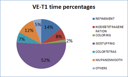
|
| Figure 135: Time percentages of different parts of the algorithm for generating the mesh of validation example . |
| Model data | |
| Sphericity | |
| Number of volumes | |
| Number of triangles input mesh | |
| Watertight | |
| Mesh size (uol) | |
| Transition factor | |
| Result mesh | |
| Number of tetrahedra | |
| Number of nodes | |
| Number of triangles (skin of tetrahedra) | |
| Number of edges | |
| Minimum dihedral angle before make-up and smoothing (degrees) | |
| Tetrahedra with min dihedral angle before make-up and smoothing | |
| Minimum dihedral angle in final mesh (degrees) | |
| Memory | |
| Memory base (Mb) | |
| Memory peak (Mb) | |
| Memory ratio | |
| Algorithm data | |
| Number of local ray casting operations | |
| Number of undetermined tetrahedra | |
| Number of tetrahedra from interface cells | |
| Number of tetrahedra after make-up and smoothing | |
| Number of octree cells (refining the whole root) | |
| Number of outer cells (refining the whole root) | |
| Number of octree cells in the current implementation | |
| Number of interface octree cells | |
| Time and speed | |
| Number of threads | |
| Total time for generating the mesh (s) | |
| Speed (Mtetrahedra per minute) | |
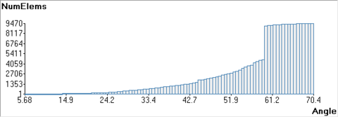
|
| Figure 136: Distribution of minimum dihedral angles in the mesh generated in the validation example . |
A.2 Validation example VE-T2
| Model data | |
| Sphericity | |
| Number of volumes | |
| Number of triangles input mesh | |
| Watertight | |
| Mesh size (uol) | |
| Transition factor | |
| Result mesh | |
| Number of tetrahedra | |
| Number of nodes | |
| Number of triangles (skin of tetrahedra) | |
| Number of edges | |
| Minimum dihedral angle before make-up and smoothing (degrees) | |
| Tetrahedra with min dihedral angle before make-up and smoothing | |
| Minimum dihedral angle in final mesh (degrees) | |
| Memory | |
| Memory base (Mb) | |
| Memory peak (Mb) | |
| Memory ratio | |
| Algorithm data | |
| Number of local ray casting operations | |
| Number of undetermined tetrahedra | |
| Number of tetrahedra from interface cells | |
| Number of tetrahedra after make-up and smoothing | |
| Number of octree cells (refining the whole root) | |
| Number of outer cells (refining the whole root) | |
| Number of octree cells in the current implementation | |
| Number of interface octree cells | |
| Time and speed | |
| Number of threads | |
| Total time for generating the mesh (s) | |
| Speed (Mtetrahedra per minute) | |
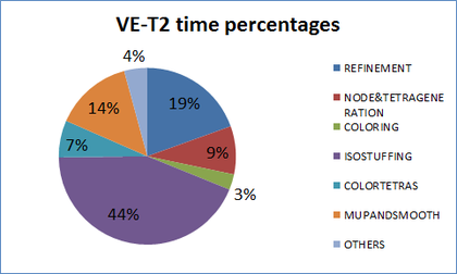
|
| Figure 137: Time percentages of different parts of the algorithm for generating the mesh of validation example . |
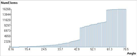
|
| Figure 138: Distribution of minimum dihedral angles in the mesh generated in the validation example . |
A.3 Validation example VE-T3
| Model data | |
| Sphericity | |
| Number of volumes | |
| Number of triangles input mesh | |
| Watertight | |
| Mesh size (uol) | |
| Transition factor | |
| Result mesh | |
| Number of tetrahedra | |
| Number of nodes | |
| Number of triangles (skin of tetrahedra) | |
| Number of edges | |
| Minimum dihedral angle before make-up and smoothing (degrees) | |
| Tetrahedra with min dihedral angle before make-up and smoothing | |
| Minimum dihedral angle in final mesh (degrees) | |
| Memory | |
| Memory base (Mb) | |
| Memory peak (Mb) | |
| Memory ratio | |
| Algorithm data | |
| Number of local ray casting operations | |
| Number of undetermined tetrahedra | |
| Number of tetrahedra from interface cells | |
| Number of tetrahedra after make-up and smoothing | |
| Number of octree cells (refining the whole root) | |
| Number of outer cells (refining the whole root) | |
| Number of octree cells in the current implementation | |
| Number of interface octree cells | |
| Time and speed | |
| Number of threads | |
| Total time for generating the mesh (s) | |
| Speed (Mtetrahedra per minute) | |
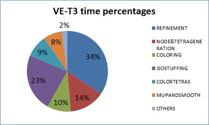
|
| Figure 139: Time percentages of different parts of the algorithm for generating the mesh of validation example . |
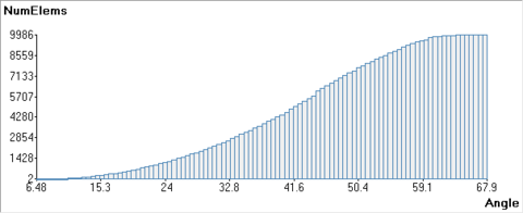
|
| Figure 140: Distribution of minimum dihedral angles in the mesh generated in the validation example . |
A.4 Validation example VE-F1
| Model data | |
| Sphericity | |
| Number of volumes | |
| Number of triangles input mesh | |
| Watertight | |
| General mesh size (uol) | |
| Mesh size in the wing surfaces (uol) | |
| Transition factor | |
| Result mesh | |
| Number of tetrahedra | |
| Number of nodes | |
| Number of triangles (skin of tetrahedra) | |
| Number of edges | |
| Minimum dihedral angle before make-up and smoothing (degrees) | |
| Tetrahedra with min dihedral angle before make-up and smoothing | |
| Minimum dihedral angle in final mesh (degrees) | |
| Tetrahedra with min dihedral angle | |
| Memory | |
| Memory base (Mb) | |
| Memory peak (Mb) | |
| Memory ratio | |
| Algorithm data | |
| Number of local ray casting operations | |
| Number of undetermined tetrahedra | |
| Number of tetrahedra from interface cells | |
| Number of tetrahedra after make-up and smoothing | |
| Number of octree cells (refining the whole root) | |
| Number of outer cells (refining the whole root) | |
| Number of octree cells in the current implementation | |
| Number of interface octree cells | |
| Time and speed | |
| Number of threads | |
| Total time for generating the mesh (s) | |
| Speed (Mtetrahedra per minute) | |
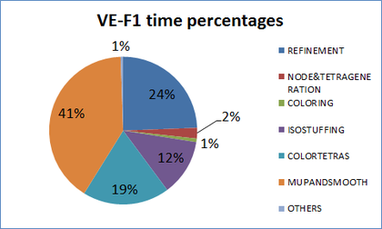
|
| Figure 141: Time percentages of different parts of the algorithm for generating the mesh of validation example . |
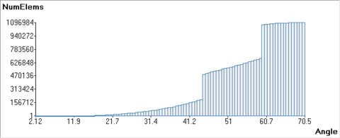
|
| Figure 142: Distribution of minimum dihedral angles in the mesh generated in the validation example . |
A.5 Validation example VE-F2
| Model data | |
| Sphericity | |
| Number of volumes | |
| Number of triangles input mesh | |
| Watertight | |
| Mesh size (uol) | |
| Transition factor | |
| Result mesh | |
| Number of tetrahedra | |
| Number of nodes | |
| Number of triangles (skin of tetrahedra) | |
| Number of edges | |
| Minimum dihedral angle before make-up and smoothing (degrees) | |
| Tetrahedra with min dihedral angle before make-up and smoothing | |
| Minimum dihedral angle in final mesh (degrees) | |
| Tetrahedra with min dihedral angle | |
| Memory | |
| Memory base (Mb) | |
| Memory peak (Mb) | |
| Memory ratio | |
| Algorithm data | |
| Number of local ray casting operations | |
| Number of undetermined tetrahedra | |
| Number of tetrahedra from interface cells | |
| Number of tetrahedra after make-up and smoothing | |
| Number of octree cells (refining the whole root) | |
| Number of outer cells (refining the whole root) | |
| Number of octree cells in the current implementation | |
| Number of interface octree cells | |
| Time and speed | |
| Number of threads | |
| Total time for generating the mesh (s) | |
| Speed (Mtetrahedra per minute) | |
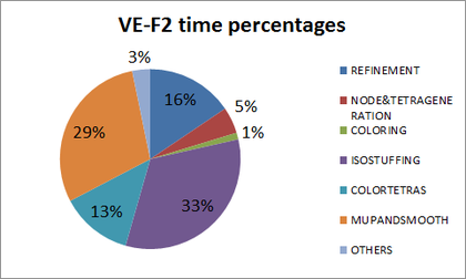
|
| Figure 143: Time percentages of different parts of the algorithm for generating the mesh of validation example . |
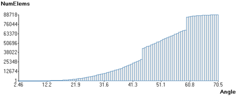
|
| Figure 144: Distribution of minimum dihedral angles in the mesh generated in the validation example . |
A.6 Validation example VE-W1
| Model data | |
| Sphericity | |
| Number of volumes | |
| Number of triangles input mesh | |
| Watertight | |
| Mesh size (uol) | |
| Transition factor | |
| Result mesh | |
| Number of tetrahedra | |
| Number of nodes | |
| Number of triangles (skin of tetrahedra) | |
| Number of edges | |
| Minimum dihedral angle before make-up and smoothing (degrees) | |
| Tetrahedra with min dihedral angle before make-up and smoothing | |
| Minimum dihedral angle in final mesh (degrees) | |
| Memory | |
| Memory base (Mb) | |
| Memory peak (Mb) | |
| Memory ratio | |
| Algorithm data | |
| Number of local ray casting operations | |
| Number of undetermined tetrahedra | |
| Number of tetrahedra from interface cells | |
| Number of tetrahedra after make-up and smoothing | |
| Number of octree cells (refining the whole root) | |
| Number of outer cells (refining the whole root) | |
| Number of octree cells in the current implementation | |
| Number of interface octree cells | |
| Time and speed | |
| Number of threads | |
| Total time for generating the mesh (s) | |
| Speed (Mtetrahedra per minute) | |
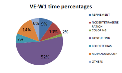
|
| Figure 145: Time percentages of different parts of the algorithm for generating the mesh of validation example . |
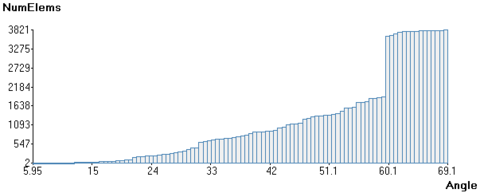
|
| Figure 146: Distribution of minimum dihedral angles in the mesh generated in the validation example . |
A.7 Validation example VE-W2
| Model data | |
| Sphericity | |
| Number of volumes | |
| Number of triangles input mesh | |
| Watertight | |
| Mesh size (uol) | |
| Transition factor | |
| Result mesh | |
| Number of tetrahedra | |
| Number of nodes | |
| Number of triangles (skin of tetrahedra) | |
| Number of edges | |
| Minimum dihedral angle before make-up and smoothing (degrees) | |
| Tetrahedra with min dihedral angle before make-up and smoothing | |
| Minimum dihedral angle in final mesh (degrees) | |
| Tetrahedra with min dihedral angle | |
| Memory | |
| Memory base (Mb) | |
| Memory peak (Mb) | |
| Memory ratio | |
| Algorithm data | |
| Number of local ray casting operations | |
| Number of undetermined tetrahedra | |
| Number of tetrahedra from interface cells | |
| Number of tetrahedra after make-up and smoothing | |
| Number of octree cells (refining the whole root) | |
| Number of outer cells (refining the whole root) | |
| Number of octree cells in the current implementation | |
| Number of interface octree cells | |
| Time and speed | |
| Number of threads | |
| Total time for generating the mesh (s) | |
| Speed (Mtetrahedra per minute) | |
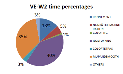
|
| Figure 147: Time percentages of different parts of the algorithm for generating the mesh of validation example . |
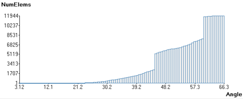
|
| Figure 148: Distribution of minimum dihedral angles in the mesh generated in the validation example . |
A.8 Validation example VE-W3
| Model data | |
| Sphericity | |
| Number of volumes | |
| Number of triangles input mesh | |
| Watertight | |
| Mesh size (uol) | |
| Transition factor | |
| Result mesh | |
| Number of tetrahedra | |
| Number of nodes | |
| Number of triangles (skin of tetrahedra) | |
| Number of edges | |
| Minimum dihedral angle before make-up and smoothing (degrees) | |
| Minimum dihedral angle in final mesh (degrees) | |
| Memory | |
| Memory base (Mb) | |
| Memory peak (Mb) | |
| Memory ratio | |
| Algorithm data | |
| Number of local ray casting operations | |
| Number of undetermined tetrahedra | |
| Number of tetrahedra from interface cells | |
| Number of tetrahedra after make-up and smoothing | |
| Number of octree cells (refining the whole root) | |
| Number of outer cells (refining the whole root) | |
| Number of octree cells in the current implementation | |
| Number of interface octree cells | |
| Time and speed | |
| Number of threads | |
| Total time for generating the mesh (s) | |
| Speed (Mtetrahedra per minute) | |
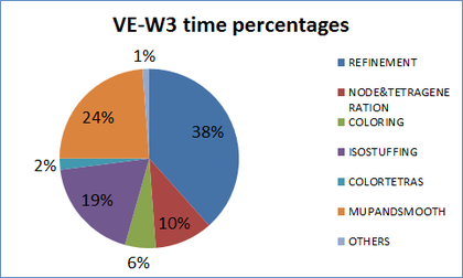
|
| Figure 149: Time percentages of different parts of the algorithm for generating the mesh of validation example . |
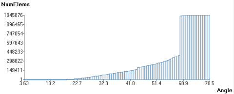
|
| Figure 150: Distribution of minimum dihedral angles in the mesh generated in the validation example . |
A.9 Validation example VE-C1
| Model data | |
| Sphericity | |
| Number of volumes | |
| Number of triangles input mesh | |
| Watertight | |
| Mesh size | |
| Transition factor | |
| Result mesh | |
| Number of tetrahedra | |
| Number of nodes | |
| Number of triangles (skin of tetrahedra) | |
| Number of edges | |
| Minimum dihedral angle before make-up and smoothing (degrees) | |
| Tetrahedra with min dihedral angle before make-up and smoothing | |
| Minimum dihedral angle in final mesh (degrees) | |
| Memory | |
| Memory base (Mb) | |
| Memory peak (Mb) | |
| Memory ratio | |
| Algorithm data | |
| Number of local ray casting operations | |
| Number of undetermined tetrahedra | |
| Number of tetrahedra from interface cells | |
| Number of tetrahedra after make-up and smoothing | |
| Number of octree cells (refining the whole root) | |
| Number of outer cells (refining the whole root) | |
| Number of octree cells in the current implementation | |
| Number of interface octree cells | |
| Time and speed | |
| Number of threads | |
| Total time for generating the mesh (s) | |
| Speed (Mtetrahedra per minute) | |
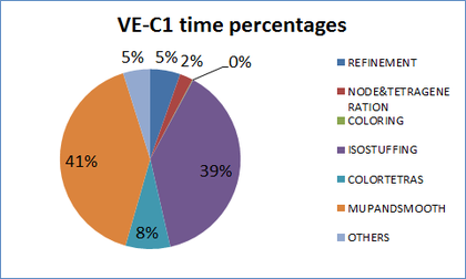
|
| Figure 151: Time percentages of different parts of the algorithm for generating the mesh of validation example . |
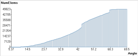
|
| Figure 152: Distribution of minimum dihedral angles in the mesh generated in the validation example . |
A.10 Validation example VE-C2
| Model data | |
| Sphericity | |
| Number of volumes | |
| Number of triangles input mesh | |
| Watertight | |
| Mesh size | |
| Transition factor | |
| Result mesh | |
| Number of tetrahedra | |
| Number of nodes | |
| Number of triangles (skin of tetrahedra) | |
| Number of edges | |
| Minimum dihedral angle before make-up and smoothing (degrees) | |
| Tetrahedra with min dihedral angle before make-up and smoothing | |
| Minimum dihedral angle in final mesh (degrees) | |
| Memory | |
| Memory base (Mb) | |
| Memory peak (Mb) | |
| Memory ratio | |
| Algorithm data | |
| Number of local ray casting operations | |
| Number of undetermined tetrahedra | |
| Number of tetrahedra from interface cells | |
| Number of tetrahedra after make-up and smoothing | |
| Number of octree cells (refining the whole root) | |
| Number of outer cells (refining the whole root) | |
| Number of octree cells in the current implementation | |
| Number of interface octree cells | |
| Time and speed | |
| Number of threads | |
| Total time for generating the mesh (s) | |
| Speed (Mtetrahedra per minute) | |
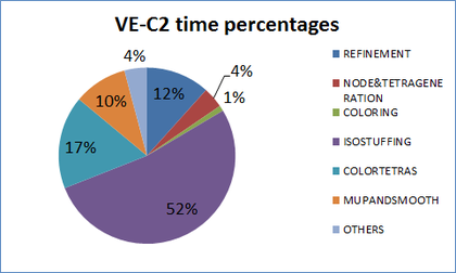
|
| Figure 153: Time percentages of different parts of the algorithm for generating the mesh of validation example . |
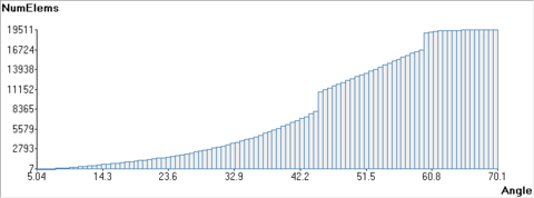
|
| Figure 154: Distribution of minimum dihedral angles in the mesh generated in the validation example . |
A.11 Validation example VE-C3
| Model data | |
| Sphericity | |
| Number of volumes | |
| Number of triangles input mesh | |
| Watertight | |
| Mesh size | |
| Transition factor | |
| Result mesh | |
| Number of tetrahedra | |
| Number of nodes | |
| Number of triangles (skin of tetrahedra) | |
| Number of edges | |
| Minimum dihedral angle before make-up and smoothing (degrees) | |
| Tetrahedra with min dihedral angle before make-up and smoothing | |
| Minimum dihedral angle in final mesh (degrees) | |
| Memory | |
| Memory base (Mb) | |
| Memory peak (Mb) | |
| Memory ratio | |
| Algorithm data | |
| Number of local ray casting operations | |
| Number of undetermined tetrahedra | |
| Number of tetrahedra from interface cells | |
| Number of tetrahedra after make-up and smoothing | |
| Number of octree cells (refining the whole root) | |
| Number of outer cells (refining the whole root) | |
| Number of octree cells in the current implementation | |
| Number of interface octree cells | |
| Time and speed | |
| Number of threads | |
| Total time for generating the mesh (s) | |
| Speed (Mtetrahedra per minute) | |
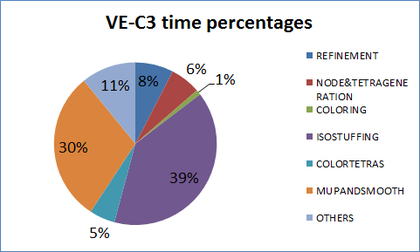
|
| Figure 155: Time percentages of different parts of the algorithm for generating the mesh of validation example . |
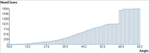
|
| Figure 156: Distribution of minimum dihedral angles in the mesh generated in the validation example . |
A.12 Validation example VE-I1
| Model data | |
| Sphericity | |
| Number of volumes | |
| Number of triangles input mesh | |
| Watertight | |
| Mesh size (uol) | |
| Transition factor | |
| Result mesh | |
| Number of tetrahedra | |
| Number of nodes | |
| Number of triangles (skin of tetrahedra) | |
| Number of edges | |
| Minimum dihedral angle before make-up and smoothing (degrees) | |
| Tetrahedra with min dihedral angle before make-up and smoothing | |
| Minimum dihedral angle in final mesh (degrees) | |
| Memory | |
| Memory base (Mb) | |
| Memory peak (Mb) | |
| Memory ratio | |
| Algorithm data | |
| Number of local ray casting operations | |
| Number of undetermined tetrahedra | |
| Number of tetrahedra from interface cells | |
| Number of tetrahedra after make-up and smoothing | |
| Number of octree cells (refining the whole root) | |
| Number of outer cells (refining the whole root) | |
| Number of octree cells in the current implementation | |
| Number of interface octree cells | |
| Time and speed | |
| Number of threads | |
| Total time for generating the mesh (s) | |
| Speed (Mtetrahedra per minute) | |
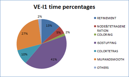
|
| Figure 157: Time percentages of different parts of the algorithm for generating the mesh of validation example . |
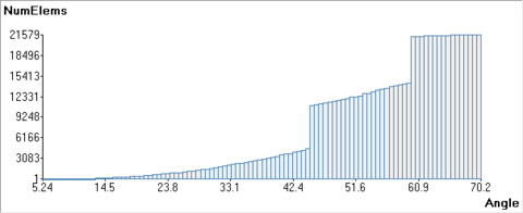
|
| Figure 158: Distribution of minimum dihedral angles in the mesh generated in the validation example . |
A.13 Validation example VE-E1
| Model data | |
| Number of volumes | |
| Number of triangles input mesh | |
| Watertight | |
| General mesh size (uol) | |
| Mesh size in the boundaries (uol) | |
| Transition factor | |
| Result mesh | |
| Number of tetrahedra | |
| Number of nodes | |
| Memory | |
| Memory base (Mb) | |
| Memory peak (Mb) | |
| Memory ratio | |
| Algorithm data | |
| Number of local ray casting operations | |
| Number of octree cells in the current implementation | |
| Number of interface octree cells | |
| Time and speed | |
| Number of threads | |
| Total time for generating the mesh (s) | |
| Speed (Mtetrahedra per minute) | |
A.14 Validation example VE-S1
| Configuration | ||||
| Model data | ||||
| Sphericity | ||||
| Number of volumes | ||||
| Number of triangles input mesh | ||||
| Watertight | ||||
| Mesh size | ||||
| Transition factor | ||||
| Result mesh | ||||
| Number of tetrahedra (millions) | ||||
| Number of nodes (millions) | ||||
| Number of triangles (skin of tetrahedra) | ||||
| Number of edges | ||||
| Min angle (mda) before smoothing (deg) | ||||
| Tetrahedra with mda before smoothing | ||||
| Min dihedral angle in final mesh (deg) | ||||
| Memory | ||||
| Memory base (Mb) | ||||
| Memory peak (Mb) | ||||
| Memory ratio | ||||
| Algorithm data | ||||
| Num of local ray casting operations | ||||
| Num of undetermined tetrahedra | ||||
| Num of tetrahedra from interface cells | ||||
| Num of tetrahedra after smoothing | ||||
| Num of octree cells (refining the whole root) | ||||
| Num of outer cells (refining the whole root) | ||||
| Num of octree cells current implementation | ||||
| Num of interface octree cells | ||||
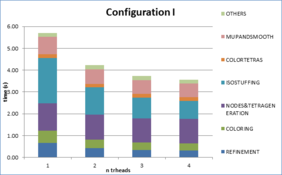
|
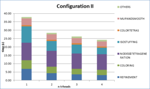
|
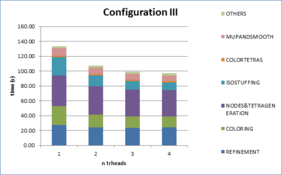
|
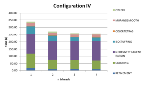
|
| Figure 159: Times consumed in the different parts of the meshing algorithm for the validation example . | |
A.15 Validation example VE-S2
| Configuration | ||||
| Model data | ||||
| Sphericity | ||||
| Number of volumes | ||||
| Number of triangles input mesh | ||||
| Watertight | ||||
| General mesh size (uol) | ||||
| Mesh size in buildings (uol) | ||||
| Transition factor | ||||
| Result mesh | ||||
| Number of tetrahedra (millions) | ||||
| Number of nodes millions) | ||||
| Number of triangles (skin of tetrahedra) | ||||
| Number of edges | ||||
| Min d. angle (mda) before smoothing (deg) | ||||
| Tetrahedra with mda before smoothing | ||||
| Min dihedral angle in final mesh (deg) | ||||
| Memory | ||||
| Memory base (Mb) | ||||
| Memory peak (Mb) | ||||
| Memory ratio | ||||
| Algorithm data | ||||
| Num of local ray casting operations | ||||
| Num of undetermined tetrahedra | ||||
| Num of tetrahedra from interface cells (M) | ||||
| Num of tetrahedra after smoothing | ||||
| Num of octree cells (refining the whole root) | ||||
| Num of outer cells (refining the whole root) | ||||
| Num of octree cells current implementation | ||||
| Num of interface octree cells | ||||
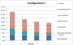
|
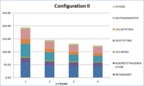
|
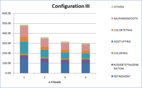
|
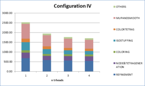
|
| Figure 160: Times consumed in the different parts of the meshing algorithm for the validation example . | |
A.16 Racing car
| Model data | |
| Sphericity | |
| Number of volumes | |
| Number of triangles input mesh | |
| Watertight | |
| Mesh general size (uol) | None |
| Mesh size in skin of the car and floor (uol) | |
| Mesh size in outlet surface (uol) | |
| Transition factor | |
| Result mesh | |
| Number of tetrahedra (millions) | |
| Number of nodes (millions) | |
| Number of triangles (skin of tetrahedra) | |
| Number of edges | |
| Minimum dihedral angle before make-up and smoothing (degrees) | |
| Tetrahedra with min dihedral angle before mesh improvement | |
| Minimum dihedral angle in final mesh (degrees) | |
| Tetrahedra with min dihedral angle | |
| Memory | |
| Memory base (Mb) | |
| Memory peak (Mb) | |
| Memory ratio | |
| Algorithm data | |
| Number of local ray casting operations | |
| Number of undetermined tetrahedra | |
| Number of tetrahedra from interface cells | |
| Number of tetrahedra after make-up and smoothing | |
| Number of octree cells (refining the whole root) | |
| Number of outer cells (refining the whole root) | |
| Number of octree cells in the current implementation | |
| Number of interface octree cells | |
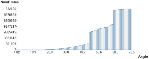
|
| Figure 161: Distribution of minimum dihedral angles in the mesh generated in the racing car example. |
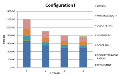
|
| Figure 162: Times consumed in the different parts of the meshing algorithm for the racing car example. |
A.17 Barcelona model
| Model data | |
| Sphericity | |
| Number of volumes | |
| Number of triangles input mesh | |
| Watertight | |
| General mesh size (uol) | |
| Mesh size in buildings (uol) | |
| Mesh size in terrain (uol) | |
| Transition factor | |
| Result mesh | |
| Number of tetrahedra (millions) | |
| Number of nodes | |
| Number of triangles (skin of tetrahedra) | |
| Number of edges | |
| Minimum dihedral angle before make-up and smoothing (degrees) | |
| Minimum dihedral angle in final mesh (degrees) | |
| Memory | |
| Memory base (Gb) | |
| Memory peak (Gb) | |
| Memory ratio | |
| Algorithm data | |
| Number of local ray casting operations | |
| Number of undetermined tetrahedra | |
| Number of tetrahedra from interface cells | |
| Number of tetrahedra after make-up and smoothing | |
| Number of octree cells (refining the whole root) | |
| Number of outer cells (refining the whole root) | |
| Number of octree cells in the current implementation | |
| Number of interface octree cells | |
Document information
Published on 13/03/18
Submitted on 13/03/18
Licence: CC BY-NC-SA license
Share this document
Keywords
claim authorship
Are you one of the authors of this document?
