| (12 intermediate revisions by the same user not shown) | |||
| Line 19: | Line 19: | ||
==Abstract== | ==Abstract== | ||
| − | Urban drainage systems are facing increasing challenges due to climate change, urban growth, and the need for more sustainable water management. To address these issues, the Digital DRAIN project has developed a tool that integrates different models within a GIS environment to analyse the performance of urban drainage systems. The tool helps assess both water flows and pollution, while also supporting the design of sustainable solutions and adaptation strategies. Delivered as the QGIS plugin IberGIS, it provides an accessible framework to improve urban water management and enhance resilience against floods and environmental impacts. | + | Urban drainage systems are facing increasing challenges due to climate change, urban growth, and the need for more sustainable water management. To address these issues, the Digital DRAIN project has developed a tool that integrates different models within a GIS environment to analyse the performance of urban drainage systems. The tool helps assess both water flows and pollution, while also supporting the design of sustainable solutions and adaptation strategies. Delivered as the QGIS plugin IberGIS, it provides an accessible framework to improve urban water management and enhance resilience against floods and environmental impacts. This document is a user's guide to introduce the user how to use IberGIS. |
'''Keywords''': urban drainage, 1D/2D modelling, Iber-SWMM, QGIS | '''Keywords''': urban drainage, 1D/2D modelling, Iber-SWMM, QGIS | ||
| Line 27: | Line 27: | ||
==Resumen== | ==Resumen== | ||
| − | Los sistemas de drenaje urbano se enfrentan a retos cada vez mayores debido al cambio climático, el crecimiento urbano y la necesidad de una gestión del agua más sostenible. Para abordar estos problemas, el proyecto Digital DRAIN ha desarrollado una herramienta que integra diversos modelos en un entorno SIG para analizar el rendimiento de los urban sistemas de drenaje. Esta herramienta permite evaluar tanto el caudal como la contaminación del agua, además de facilitar el diseño de soluciones sostenibles y estrategias de adaptación. Implementada como complemento de QGIS, IberGIS ofrece un marco accesible para mejorar la gestión del agua urbana y aumentar la resiliencia ante inundaciones e impactos ambientales. | + | Los sistemas de drenaje urbano se enfrentan a retos cada vez mayores debido al cambio climático, el crecimiento urbano y la necesidad de una gestión del agua más sostenible. Para abordar estos problemas, el proyecto Digital DRAIN ha desarrollado una herramienta que integra diversos modelos en un entorno SIG para analizar el rendimiento de los urban sistemas de drenaje. Esta herramienta permite evaluar tanto el caudal como la contaminación del agua, además de facilitar el diseño de soluciones sostenibles y estrategias de adaptación. Implementada como complemento de QGIS, IberGIS ofrece un marco accesible para mejorar la gestión del agua urbana y aumentar la resiliencia ante inundaciones e impactos ambientales. Este documento es una guía de usaurio para introducir al usuario en el manejo de IberGIS. |
'''Palabras clave''': drenaje urbano, simulación 1D/2D, Iber-SWMM, QGIS | '''Palabras clave''': drenaje urbano, simulación 1D/2D, Iber-SWMM, QGIS | ||
| Line 218: | Line 218: | ||
|- | |- | ||
| style="text-align: center;width: 45%;"|[[File:Sanz-Ramos_et_al_2025a_1020_Fig_4a.png|1600px]] | | style="text-align: center;width: 45%;"|[[File:Sanz-Ramos_et_al_2025a_1020_Fig_4a.png|1600px]] | ||
| − | | style="text-align: center;width: | + | | style="text-align: center;width: 35%;"|[[File:Sanz-Ramos_et_al_2025a_6524_Fig_4b.png|1600px]] |
|- | |- | ||
| style="text-align: center;"|(a) | | style="text-align: center;"|(a) | ||
| Line 225: | Line 225: | ||
{| style="width: 80%;margin: 1em auto 0.1em auto;border-collapse: collapse;" | {| style="width: 80%;margin: 1em auto 0.1em auto;border-collapse: collapse;" | ||
|- | |- | ||
| − | | style="text-align: center;width: | + | | style="text-align: center;width: 40%;"|[[File:Sanz-Ramos_et_al_2025a_8408_Fig_4c.png|1600px]] |
| style="text-align: center;width: 45%;"|[[File:Sanz-Ramos_et_al_2025a_2187_Fig_4d.png|1600px]] | | style="text-align: center;width: 45%;"|[[File:Sanz-Ramos_et_al_2025a_2187_Fig_4d.png|1600px]] | ||
|- | |- | ||
| Line 282: | Line 282: | ||
The results of the numerical models, SWMM and Iber, can be shown directly in QGIS. In this case, only the 2D results of Iber are available since none sewer network has been simulated through SWMM. Fig. 7 shows the map of flow depth and velocity at the end of the simulation. As expected, the inlet subtracts water from the model surface, affecting the hydrodynamics near the inlet location. The flow accelerates when it approaches to the inlet (Fig. 7b), especially in the X direction (Fig. 7c) while the velocity in the Y direction is almost null except near the inlet. | The results of the numerical models, SWMM and Iber, can be shown directly in QGIS. In this case, only the 2D results of Iber are available since none sewer network has been simulated through SWMM. Fig. 7 shows the map of flow depth and velocity at the end of the simulation. As expected, the inlet subtracts water from the model surface, affecting the hydrodynamics near the inlet location. The flow accelerates when it approaches to the inlet (Fig. 7b), especially in the X direction (Fig. 7c) while the velocity in the Y direction is almost null except near the inlet. | ||
| − | + | {| style="width: 80%;margin: 1em auto 0.1em;border-collapse: collapse;" | |
| − | {| style="width: 80%;margin: 1em auto 0.1em | + | |
|- | |- | ||
| − | | style="text-align: center;width: | + | | style="text-align: center;width: 40%;"|[[File:Sanz-Ramos_et_al_2025a_6546_Fig_7a.png|1600px]] |
| + | | style="text-align: center;width: 5%;"|[[File:Sanz-Ramos_et_al_2025a_8202_Fig_7aa.png|1600px]] | ||
| + | | style="text-align: center;width: 40%;"|[[File:Sanz-Ramos_et_al_2025a_4592_Fig_7b.png|1600px]] | ||
| + | | style="text-align: center;width: 5%;"|[[File:Sanz-Ramos_et_al_2025a_7013_Fig_7bb.png|1600px]] | ||
|- | |- | ||
| − | | style="text-align: center;width: | + | | style="text-align: center;"|(a) |
| + | | style="text-align: center;"| | ||
| + | | style="text-align: center;"|(b) | ||
| + | | style="text-align: center;"| | ||
| + | |} | ||
| + | {| style="width: 80%;margin: 1em auto 0.1em;border-collapse: collapse;" | ||
| + | |- | ||
| + | | style="text-align: center;width: 40%;"|[[File:Sanz-Ramos_et_al_2025a_7344_Fig_7c.png|1600px]] | ||
| + | | style="text-align: center;width: 5%;"|[[File:Sanz-Ramos_et_al_2025a_9148_Fig_7cc.png|1600px]] | ||
| + | | style="text-align: center;width: 40%;"|[[File:Sanz-Ramos_et_al_2025a_2218_Fig_7d.png|1600px]] | ||
| + | | style="text-align: center;width: 5%;"|[[File:Sanz-Ramos_et_al_2025a_4909_Fig_7dd.png|1600px]] | ||
| + | |- | ||
| + | | style="text-align: center;"|(c) | ||
| + | | style="text-align: center;"| | ||
| + | | style="text-align: center;"|(d) | ||
| + | | style="text-align: center;"| | ||
|} | |} | ||
<span style="text-align: center; font-size: 75%;">'''Fig. 7. Results at the end of the simulation: (a) flow depth; (b) flow velocity (modulus); (c) flow velocity in the X direction; (d) flow velocity in the Y direction.'''</span> | <span style="text-align: center; font-size: 75%;">'''Fig. 7. Results at the end of the simulation: (a) flow depth; (b) flow velocity (modulus); (c) flow velocity in the X direction; (d) flow velocity in the Y direction.'''</span> | ||
| Line 414: | Line 431: | ||
{| style="width: 80%;margin: 1em auto 0.1em auto;border-collapse: collapse;" | {| style="width: 80%;margin: 1em auto 0.1em auto;border-collapse: collapse;" | ||
|- | |- | ||
| − | | style="text-align: center;width: | + | | style="text-align: center;width: 80%;"|[[File:Sanz-Ramos_et_al_2025a_7596_Fig_13a.png|1600px]] |
| + | | style="text-align: center;width: 10%;"|[[File:Sanz-Ramos_et_al_2025a_9294_Fig_13aa.png|1600px]] | ||
|- | |- | ||
| − | | style="text-align: center;width: | + | | style="text-align: center;"|(a) |
| + | | style="text-align: center;"| | ||
| + | |} | ||
| + | {| style="width: 80%;margin: 1em auto 0.1em auto;border-collapse: collapse;" | ||
| + | |- | ||
| + | | style="text-align: center;width: 80%;"|[[File:Sanz-Ramos_et_al_2025a_4065_Fig_13b.png|1600px]] | ||
| + | | style="text-align: center;width: 10%;"|[[File:Sanz-Ramos_et_al_2025a_3111_Fig_13bb.png|1600px]] | ||
| + | |- | ||
| + | | style="text-align: center;"|(b) | ||
| + | | style="text-align: center;"| | ||
|} | |} | ||
<span style="text-align: center; font-size: 75%;">'''Fig. 13. Results of maximums at the end of the simulation: (a) flow depth; (b) flow velocity (modulus).'''</span> | <span style="text-align: center; font-size: 75%;">'''Fig. 13. Results of maximums at the end of the simulation: (a) flow depth; (b) flow velocity (modulus).'''</span> | ||
| Line 515: | Line 542: | ||
===3.3.6 Run configuration=== | ===3.3.6 Run configuration=== | ||
| − | Once the simulation ends, accept loading the results of the simulation and, then, visualize them at 1 h of simulation. Fig. | + | Once the simulation ends, accept loading the results of the simulation and, then, visualize them at 1 h of simulation. Fig. 17 shows the map of water depth and flow velocity (modulus) on the surface (results of Iber), and how the flow is transported over the streets mainly to the NE direction (where the outlet conditions are implemented). Considerable water accumulation is produced in five to nine locations (Fig. 18a) due to topographical depressions and the no consideration of outlet conditions (e.g., at southern part of the model). |
{| style="width: 80%;margin: 1em auto 0.1em auto;border-collapse: collapse;" | {| style="width: 80%;margin: 1em auto 0.1em auto;border-collapse: collapse;" | ||
|- | |- | ||
| − | | style="text-align: center;width: | + | | style="text-align: center;width: 80%;"|[[File:Sanz-Ramos_et_al_2025a_8124_Fig_17a.png|1600px]] |
| + | | style="text-align: center;width: 10%;"|[[File:Sanz-Ramos_et_al_2025a_3871_Fig_17aa.png|1600px]] | ||
| + | |- | ||
| + | | style="text-align: center;"|(a) | ||
| + | | style="text-align: center;"| | ||
|} | |} | ||
| − | <span style="text-align: center; font-size: 75%;">'''Fig. | + | {| style="width: 80%;margin: 1em auto 0.1em auto;border-collapse: collapse;" |
| + | |- | ||
| + | | style="text-align: center;width: 80%;"|[[File:Sanz-Ramos_et_al_2025a_3399_Fig_17b.png|1600px]] | ||
| + | | style="text-align: center;width: 10%;"|[[File:Sanz-Ramos_et_al_2025a_3293_Fig_17bb.png|1600px]] | ||
| + | |- | ||
| + | | style="text-align: center;"|(b) | ||
| + | | style="text-align: center;"| | ||
| + | |} | ||
| + | <span style="text-align: center; font-size: 75%;">'''Fig. 17. Hydrodynamic results on surface 1 h after the simulation starts: (a) depths; (b) velocities.'''</span> | ||
| − | We can also check the Report summary of SWMM results. Fig. | + | We can also check the Report summary of SWMM results. Fig. 18 shows an example for node depths, node inflows, link flows and outfall loading. Junction J60 presents a maximum depth of 3.55 m; thus, this node is under pressure and the flow goes from the sewer network to the street (this is one of the causes of water accumulation there, see Fig. 18a). In Node subcharge option we can observe that this node is working in pressurized flow for more than 2 hours. |
The outfall that spills the maximum discharge is O1, located at NE, with a peak discharge above 0.06 m3/s. This is because the sewer network mainly drains into this direction, and the flow in the conduits tends to accumulate in such direction. | The outfall that spills the maximum discharge is O1, located at NE, with a peak discharge above 0.06 m3/s. This is because the sewer network mainly drains into this direction, and the flow in the conduits tends to accumulate in such direction. | ||
| Line 529: | Line 568: | ||
{| style="width: 80%;margin: 1em auto 0.1em auto;border-collapse: collapse;" | {| style="width: 80%;margin: 1em auto 0.1em auto;border-collapse: collapse;" | ||
|- | |- | ||
| − | | style="text-align: center;width: | + | | style="text-align: center;width: 25%;"|[[File:Sanz-Ramos_et_al_2025a_7003_Fig_19a.png|1600px]] |
| + | | style="text-align: center;width: 25%;"|[[File:Sanz-Ramos_et_al_2025a_1932_Fig_19b.png|1600px]] | ||
| + | | style="text-align: center;width: 25%;"|[[File:Sanz-Ramos_et_al_2025a_3713_Fig_19c.png|1600px]] | ||
| + | | style="text-align: center;width: 25%;"|[[File:Sanz-Ramos_et_al_2025a_9956_Fig_19d.png|1600px]] | ||
| + | |- | ||
| + | | style="text-align: center;"|(a) | ||
| + | | style="text-align: center;"|(b) | ||
| + | | style="text-align: center;"|(c) | ||
| + | | style="text-align: center;"|(d) | ||
|} | |} | ||
| − | <span style="text-align: center; font-size: 75%;">'''Fig. | + | <span style="text-align: center; font-size: 75%;">'''Fig. 18. Hydrodynamic results in the sewer network (Summary report): (a) node depths; (b) node inflow; (c) link flow; (d) outfall loading.'''</span> |
==Funding== | ==Funding== | ||
Latest revision as of 06:15, 14 November 2025
Abstract
Urban drainage systems are facing increasing challenges due to climate change, urban growth, and the need for more sustainable water management. To address these issues, the Digital DRAIN project has developed a tool that integrates different models within a GIS environment to analyse the performance of urban drainage systems. The tool helps assess both water flows and pollution, while also supporting the design of sustainable solutions and adaptation strategies. Delivered as the QGIS plugin IberGIS, it provides an accessible framework to improve urban water management and enhance resilience against floods and environmental impacts. This document is a user's guide to introduce the user how to use IberGIS.
Keywords: urban drainage, 1D/2D modelling, Iber-SWMM, QGIS
Resumen
Los sistemas de drenaje urbano se enfrentan a retos cada vez mayores debido al cambio climático, el crecimiento urbano y la necesidad de una gestión del agua más sostenible. Para abordar estos problemas, el proyecto Digital DRAIN ha desarrollado una herramienta que integra diversos modelos en un entorno SIG para analizar el rendimiento de los urban sistemas de drenaje. Esta herramienta permite evaluar tanto el caudal como la contaminación del agua, además de facilitar el diseño de soluciones sostenibles y estrategias de adaptación. Implementada como complemento de QGIS, IberGIS ofrece un marco accesible para mejorar la gestión del agua urbana y aumentar la resiliencia ante inundaciones e impactos ambientales. Este documento es una guía de usaurio para introducir al usuario en el manejo de IberGIS.
Palabras clave: drenaje urbano, simulación 1D/2D, Iber-SWMM, QGIS
1 Introduction
In recent years, the planning, design, construction, and management of urban drainage elements has evolved towards an integrated approach, known as dual drainage. This process focuses on the joint understanding of all physical processes involved, both in terms of water quantity and quality, as well as surface and sewer network flows, and the final receiving environment (rivers, estuaries, seas, and oceans). This requires modelling and analysis tools that account for such coupling (dual drainage). Furthermore, these tools must address today’s global challenges, moving towards a more sustainable world, improving the ecological status of the environment, incorporating climate change adaptation strategies, and ensuring public safety in the face of natural phenomena such as floods.
Along these lines, the project entitled ‘Digital DRAIN. An Integrated Urban Drainage Model’ (DRAIN, CPP2021-008756) aims to develop an open-source, free modelling tool for analysing all processes of urban drainage, integrated within a graphical information system (GIS) environment. Its purpose is to assess hydraulic performance and the effects of diffuse pollution both on the surface, within the drainage network, and in the receiving environment. The tool will also include specific modules for the implementation of Sustainable Urban Drainage Systems (SuDS) and for analysing actions related to climate change adaptation.
The project derived in a plugin of QGIS, called IberGIS. This plugin is a full integration of the one-dimensional urban drainage software SWMM and an integration of the two-dimensional hydrodynamic software Iber, particularly its calculation module Iber-SWMM [1]. Thus, not all capabilities neither calculation modules of Iber are available. Only particular characteristics of the Iber-SWMM module are described below.
QGIS plugin
IberGIS can be freely downloaded through www.iberaula.com.
Data
Data to build-up the models presented in this document is stored here.
Important note
This document does not attempt to be a QGIS manual. Despite the whole model’s build-up process is properly defined, the input data might require a pre-process and previous knowledge in GIS environments. The authors encourage users to familiarise with QGIS by reading the documentation and, in case of general doubts, by contacting to the community.
2 Graphical user interface of IberGIS
2.1 Generalities
The graphical user interface (GUI) of the plugin IberGIS has been developed within the QGIS environment (version 3.40 or greater), and it follows its visual style guide. As for any plugin of QGIS, IberGIS can be installed through Plugins >> Manage and Install Plugins menu and install it loading the *.zip file available from www.iberaula.com. Once installed, and according to the User’s Profile, it will be loaded automatically during the QGIS initialization.
The calculation engine, Iber-SWMM, used in this plugin corresponds to the version of Iber 3.4.0. Older versions are not compatible, while future versions might not be fully compatible.
2.2 Particularities
2.2.1 Model structure
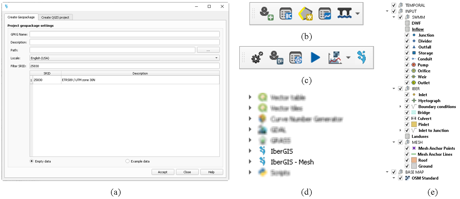
The IberGIS has a workflow fully integrated in the QGIS software. Once installed, the IberGIS button (![]() ) will automatically appear in the toolbars of QGIS. Clicking there, a new window will ask for the geopackage and QGIS project creation (Fig. 1a).
) will automatically appear in the toolbars of QGIS. Clicking there, a new window will ask for the geopackage and QGIS project creation (Fig. 1a).
After that, two new groups of toolbars of IberGIS will appear. One is related to the model’s build-up process (Fig. 1b) and the other to the model’s configuration, checks, run the simulation and visualize the results (Fig. 1c). A brief description of each option is detailed below:
- Import INP (
 ). Imports the *.inp and *.ini files of any SWMM model.
 - Boundary conditions manager (
 ). Window that enables saving different boundary condition scenarios.
 - Create boundary condition (
 ). It automatizes the implementation of boundary conditions.
 - Non visual objects manager (
 ). Window that enables saving different non visual objects, such as timeseries, rules, etc.
 - Bridges actions (
 ). Options to implement and edit bridges.
 - Options (
 ). Main model options window.
 - Generate INP (
 ). Exports the current SWMM layers to a SWMM project.
 - Mesh manager (
 ). Window that enables saving different calculation mesh scenarios.
 - Execute model (
 ). Window that enables defining general options, selecting the calculation mesh and launch the simulation.
 - Results (
 ). Options to visualize the SWMM and Iber results.
 - Check project (
 ). Dialog that starts a check project.
Additionally, the Processing Toolbox will show two specific option for IberGIS plugin (Fig. 1d). Processing Toolbox >> IberGIS is related to automatize general procedures such as project checking, import necessary features (ground, roof, inlets layers), import results, and associate Iber inlets/roofs to SWMM junctions. The other one, accessible though 'Processing Toolbox >> IberGIS – Mesh, is a pack of particular options to obtain a well-conditioned calculation mesh.
|
Fig. 1. IberGIS workflow: (a) geopackage and project creation window; (b) build-up processing toolbar; (c) other options toolbar; (d) processing toolbox of IberGIS; (e) layers structure.
Note that any IberGIS model is saved in two files: a geopackage and the QGIS project. Both are linked and when the user opens the QGIS project, automatically it will look for the geopackage. Additionally, the geopackage contains the model itself, so the user can share it without the QGIS project.
2.2.2 Workflow
All these options and functionalities are oriented to facilitate the model build-up process. Since the model is saved in a unique geopackage, different kind of entities can be saved on it. On one hand, non-visual objects is managed in the abovementioned option (![]() ). On the other hand, the creation and edition of visual objects is based on a strict group of layers (Fig. 1e) that contains TEMPORAL information (e.g., meshes, results), INPUT data (e.g., data of SWMM and Iber models) and a BASE MAP image. It is mandatory to preserve the structure of the INPUT group, since other data saved in different layers will be omitted during the calculation process:
). On the other hand, the creation and edition of visual objects is based on a strict group of layers (Fig. 1e) that contains TEMPORAL information (e.g., meshes, results), INPUT data (e.g., data of SWMM and Iber models) and a BASE MAP image. It is mandatory to preserve the structure of the INPUT group, since other data saved in different layers will be omitted during the calculation process:
INPUT
- SWMM
- Junction (layer of points)
- Divider (layer of points)
- Outfall (layer of points)
- Storage (layer of points)
- Conduit (layer of lines)
- Pump (layer of lines)
- Orifice (layer of lines)
- Weir (layer of lines)
- Outlet (layer of lines)
- IBER
- Inlet (layer of points)
- Hyetograph (layer of points)
- Boundary conditions (layer of lines)
- Bridge (layer of lines)
- Culvert (layer of lines)
- Pinlet (layer of surfaces)
- Landuses (layer of dataset)
- MESH
- Mesh anchor points (layer of points)
- Mesh anchor lines (layer of lines)
- Roof (layer of surfaces)
- Ground (layer of surfaces)
The generation of this group of layers is automatic during the models creation. It can be edit manually, using the available tools of QGIS, or automatically, using the tools of IberGIS developed ad-hoc (Fig. 1d). Thus, a manual edition requires the generation of the geometric entities of some layer of INPUT group. I.e., if the user wants to simulate only a SWMM model, the proper layer must contain all the information together with the IBER and MESH data. Whereas, an Iber model, without sewer network, requires the definition of, at least, Ground and Boundary conditions layers. Roof layer is optional and when exists it can be linked directly to the Ground or to the Junction layer (if an Iber-SWMM model is simulated). In this sense, an Iber-SWMM model, i.e., a coupled urban drainage simulation, also requires the definition of the Inlet layer and, if there is no flow, the definition of the rainfall data, whether it is by hyetographs or rasters of rain.
It is worth noticing that raster data as topography or infiltration losses can be added to any layer’s group. During the Mesh generation process (![]() ) these data, if exists in the project, can be selected. Other raster data, such as rainfall raster, must be defined as a timeseries (
) these data, if exists in the project, can be selected. Other raster data, such as rainfall raster, must be defined as a timeseries (![]() ) by defining the raster name per each time interval. The directory where the raster are located must be provided.
) by defining the raster name per each time interval. The directory where the raster are located must be provided.
Previous to the simulation process (![]() ), a new folder will be created containing the files that calculation engine Iber-SWMM will be used to carry out the simulation, even save the results. As each simulation scenario can be saved independently, different folders will be created. Note if you share the model (*.gpkg and/or *.gps), the folder that contains the results will be lost. So, the model must be re-simulated to generate again the results or consider to share all this information together with the model.
), a new folder will be created containing the files that calculation engine Iber-SWMM will be used to carry out the simulation, even save the results. As each simulation scenario can be saved independently, different folders will be created. Note if you share the model (*.gpkg and/or *.gps), the folder that contains the results will be lost. So, the model must be re-simulated to generate again the results or consider to share all this information together with the model.
2.2.3 Calculation engine
IberGIS uses the calculation engine of Iber and SWMM, and it is particularly oriented to coupled simulations using the integrated module called Iber-SWMM [1]. The urban drainage models usually require high computational effort, especially in large urban areas, the computational time can be an enormous bottleneck. To solve this issue, the simulations are carried out using the parallelised version of Iber-SWMM for NVIDIA graphical processing units (GPU) [2]. This allows accelerations in the computational time from 27 to 250 times faster than the single-threaded version.
Both models are freely distributed:
- SWMM: https://www.epa.gov/water-research/storm-water-management-model-swmm
- Iber: https://www.iberaula.com/
2.3 Current and future versions
As above-mentioned, the current version of IberGIS is particularly oriented to address flood scenarios in urban environments using, in a coupled way, two computational engines: Iber for the rainfall-runoff process and SWMM for the sewer network. Full capabilities and functionalities of the calculation engines are not currently available.
SWMM cannot be run independently since the rainfall-runoff process is carried out by Iber. Future versions might deal with these casuistic by generating a coupled and dual model, part of them being simulated with SWMM and the rest with Iber-SWMM.
Iber currently has 9 calculation modules [3] that works together with the hydrodynamic one, the principal module which the others depends on it. Only functionalities oriented to urban drainage of Iber-SWMM module are currently implemented in IberGIS. Despite that, some other functionalities, especially those related to the general hydrodynamics in flood scenarios assessment, are implemented such as bridges and culverts. Future versions might include other calculation modules of Iber.
3 Study cases
This User’s tutorial is composed by three examples: two real laboratory facility tests and a synthetic case. It is oriented to provide the elemental steps to build-up an IberGIS model, mainly to apply the Iber-SWMM calculation module for urban drainage applications.
3.1 Laboratory case: grate inlet testing platfrom
The experiment facility, located in the Hydraulic and Fluid Mechanics Laboratory of the Polytechnic University of Catalonia (UPC-BarcelonaTECH), consists in a 1:1-scale platform of 5.5 m-length and 3 m-width that represents the roadway of a street. This facility can be feed by a constant discharge up to 200 L/s and it can change its longitudinal and transverse slopes from 0 to 10 % and 0 to 4 %, respectively. It was originally designed to test the efficiency of longitudinal and transversal grate inlets [4-10]; nowadays, it is used to assess hazard criteria for objects that can be floated and transported during rainfall events in urban environments [11-14]. This exercise aims of familiarizing the user with the graphical interface and the structure of the layer, and to present other relevant information.
3.1.1 Data
The model will be build-up using the tools developed ad-hoc to facilitate the whole process. To that end, the following geometric entities are provided:
- Coordinates of the geometric entity (text)
None additional geometric information is needed since the model will be created manually.
3.1.2 Model build-up
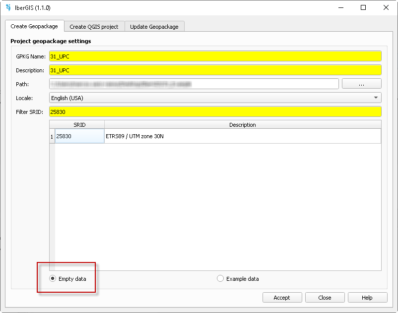
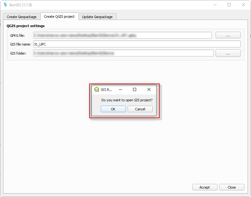
Once opened QGIS, load the IberGIS plugin by clicking on the icon ![]() , and the model generation window will appear (Fig. 2a). Please, enter the model name (GPKG Name) and a description. Then, define the location and the coordinate system using the Spatial Reference System Identifier (SRID) —in this case 25830— and click the Accept button. After that, IberGIS asks for the QGIS project creation (Fig. 2b). This step is mandatory since it will automatically load the geopackage into the QGIS project
, and the model generation window will appear (Fig. 2a). Please, enter the model name (GPKG Name) and a description. Then, define the location and the coordinate system using the Spatial Reference System Identifier (SRID) —in this case 25830— and click the Accept button. After that, IberGIS asks for the QGIS project creation (Fig. 2b). This step is mandatory since it will automatically load the geopackage into the QGIS project
|
|
| (a) | (b) |
Fig. 2. Model generation window: (a) creation of the geopackage tab; (b) creation of the QGIS project tab.
The geometry of the facility is defined by 8 points that we have to load as Delimited Text Layer by the menu Layer >> Add Layer >> Delimited Text Layer. Now, we have to select start editing (![]() ) the layer called ‘Ground’ located in the group INPUT > IBER, which contains the main information of model geometry. Add Polygon Feature (
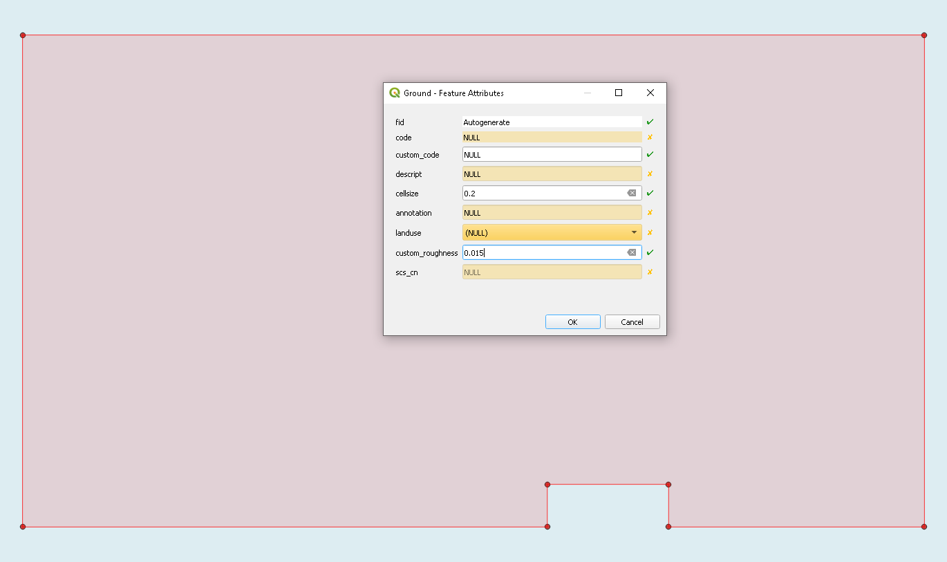
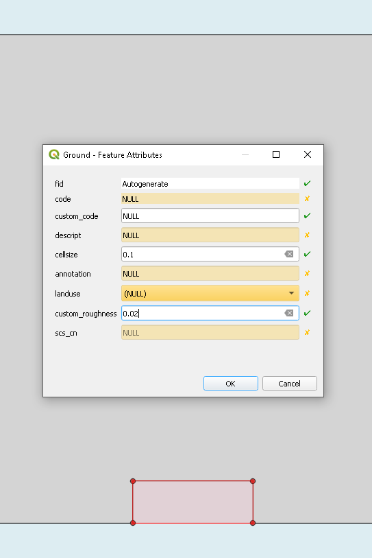
) the layer called ‘Ground’ located in the group INPUT > IBER, which contains the main information of model geometry. Add Polygon Feature (![]() ) by selecting the imported points and creating a polygon that represents the street part of the laboratory facility platform (Fig. 3). After finishing the geometry, the Feature Attribute table of ‘Ground’ layer will appear asking for the geometry properties. We can introduce a ‘cellsize’ of 0.2 m and a ‘custom_roughness’ of 0.015 s·m-1/3 (Fig. 3a). Repeat this action to create the polygon that represents de grate inlet geometry and introducing a ‘cellsize’ and ‘custom_roughness’ of 0.1 m and 0.02, respectively (Fig. 3b). Finish editing mode to save the changes into ‘Ground’ layer. Note, ‘Enable Snapping’ (
) by selecting the imported points and creating a polygon that represents the street part of the laboratory facility platform (Fig. 3). After finishing the geometry, the Feature Attribute table of ‘Ground’ layer will appear asking for the geometry properties. We can introduce a ‘cellsize’ of 0.2 m and a ‘custom_roughness’ of 0.015 s·m-1/3 (Fig. 3a). Repeat this action to create the polygon that represents de grate inlet geometry and introducing a ‘cellsize’ and ‘custom_roughness’ of 0.1 m and 0.02, respectively (Fig. 3b). Finish editing mode to save the changes into ‘Ground’ layer. Note, ‘Enable Snapping’ (![]() ) option will facilitate the creation of the model.
) option will facilitate the creation of the model.
|
|
| (a) | (b) |

|
| (c) |
Fig. 3. ‘Ground’ layer creation: (a) generation of the platform geometry; (b) generation of the grate inlet geometry; (c) View of the attribute table of ‘Ground’ layer.
This geometry corresponds to the grate inlet called ‘Barcelona1’, commonly used in Barcelona city and already experimentally and numerically tested in this facility (e.g., [9,10,15-17]). Open the attribute table of ‘Ground’ layer to verify that, indeed, the geometry is properly saved together with the properties that we defined previously (Fig. 3c). Now, we can edit both the geometry and the properties of each geometrical feature of this layer.
We can hide or delete the auxiliary layer of points used to create the polygons of ‘Ground’ layer.
3.1.3 Hydraulic conditions
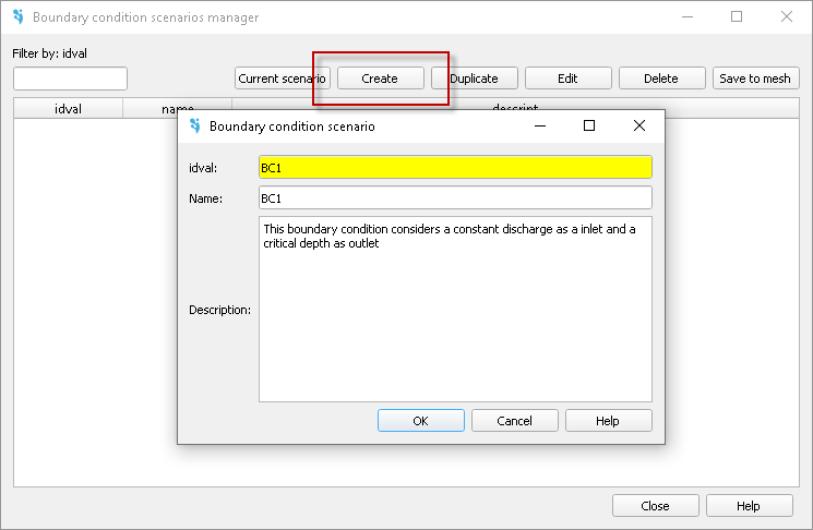
The hydraulic conditions of the model are a constant discharge (left side of the model), as inlet, and a critical flow regime (right side of the model), as outlet. To implement so, we have to open the Boundary conditions manager (![]() ) and create a new by defining the ‘idval’ code (Fig. 4a). The ‘idval’ is a mandatory parameter, ‘name’ and ‘description’ are optional. IberGIS automatically will use this ‘idval’ as ‘Current scenario’. The manager window allows to store different inlet and outlet boundary conditions per scenario using the same ‘idval’ code.
) and create a new by defining the ‘idval’ code (Fig. 4a). The ‘idval’ is a mandatory parameter, ‘name’ and ‘description’ are optional. IberGIS automatically will use this ‘idval’ as ‘Current scenario’. The manager window allows to store different inlet and outlet boundary conditions per scenario using the same ‘idval’ code.
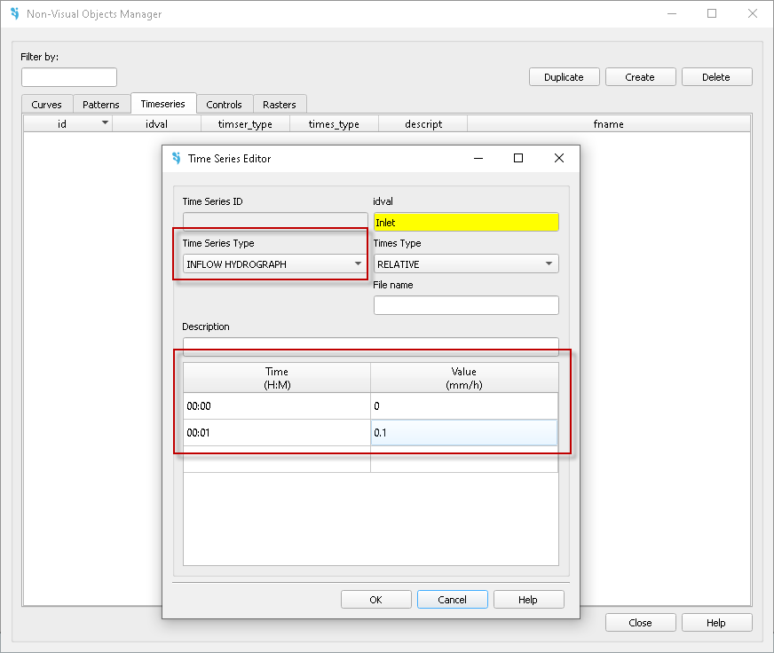
Before creating the boundary conditions, especially those that use a timeseries like as inlet condition defined by a hydrograph, we must create previously a timeseries through Non visual object manager window (![]() ). Go to ‘Timeseries’ tab and create the inlet condition by defining an increasing discharge from 0 to 0.1 m3/s in 60 s (Fig. 4b).
). Go to ‘Timeseries’ tab and create the inlet condition by defining an increasing discharge from 0 to 0.1 m3/s in 60 s (Fig. 4b).
The definition of the inlet/outlet condition can be carried out using the common options of QGIS by editing the layer called ‘Boundary conditions’. Select this layer and enable the editing mode (![]() ). Then, create a line (
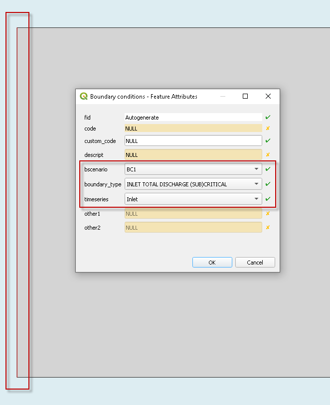
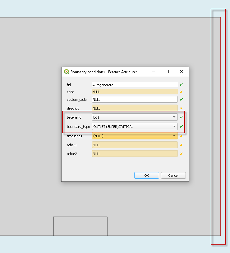
). Then, create a line (![]() ) that define the inlet boundary condition in the left side, as it is shown in Fig. 4c. In the Feature Attribute table of Boundary conditions select both the ‘bcscenario’ (BC1), ‘boundary_type’ (INLET TOTAL DISCHARGE (SUB)CRITICAL) and the ‘timeseries’ (Inlet). Repeat this process by selecting the opposite side for the outlet condition and defining the ‘bcscenario’ and the ‘boundary_type’ as BC1 and OUTLET (SUPER)CRITICAL, respectively (Fig. 4d). Finish the edition mode and save it.
) that define the inlet boundary condition in the left side, as it is shown in Fig. 4c. In the Feature Attribute table of Boundary conditions select both the ‘bcscenario’ (BC1), ‘boundary_type’ (INLET TOTAL DISCHARGE (SUB)CRITICAL) and the ‘timeseries’ (Inlet). Repeat this process by selecting the opposite side for the outlet condition and defining the ‘bcscenario’ and the ‘boundary_type’ as BC1 and OUTLET (SUPER)CRITICAL, respectively (Fig. 4d). Finish the edition mode and save it.
|
|
| (a) | (b) |
|
|
| (c) | (d) |
Fig. 4. Boundary conditions. (a) Creation of the current scenario. (b) Creation of the timeseries of the inlet conditions. (c) Implementation of the Inlet boundary condition. (d) Implementation of the Outlet boundary condition.
We are going to reproduce a grate inlet test; thus, we must define it by editing the ‘Inlet’ layer. Start editing (![]() ) and create (
) and create (![]() ) the inlet by selecting the centroid of the grate inlet surface. A Feature Attribute table will appear and we have to fill it by selecting the ‘outlet_type’ as SINK, a ‘top_elev’ of 0 m, a ‘width’ of 0.26 m, a ‘length’ of 0.74 m, the ‘method’ as W_O (i.e., weir/orifice), a ‘weir_cd’ of 1.6, a ‘orifice_cd’ of 0.7, and a ‘efficiency’ of 100. The rest of parameters by default. Save the changes.
) the inlet by selecting the centroid of the grate inlet surface. A Feature Attribute table will appear and we have to fill it by selecting the ‘outlet_type’ as SINK, a ‘top_elev’ of 0 m, a ‘width’ of 0.26 m, a ‘length’ of 0.74 m, the ‘method’ as W_O (i.e., weir/orifice), a ‘weir_cd’ of 1.6, a ‘orifice_cd’ of 0.7, and a ‘efficiency’ of 100. The rest of parameters by default. Save the changes.
3.1.4 Mesh generation
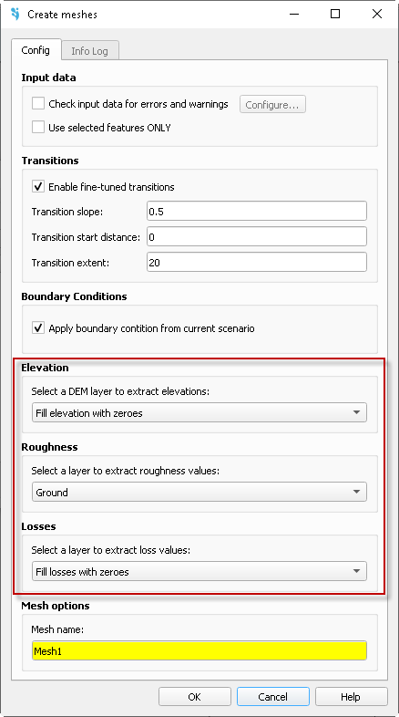
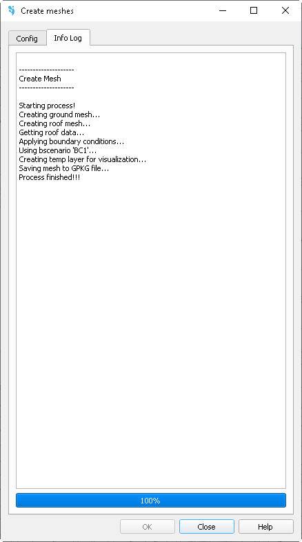
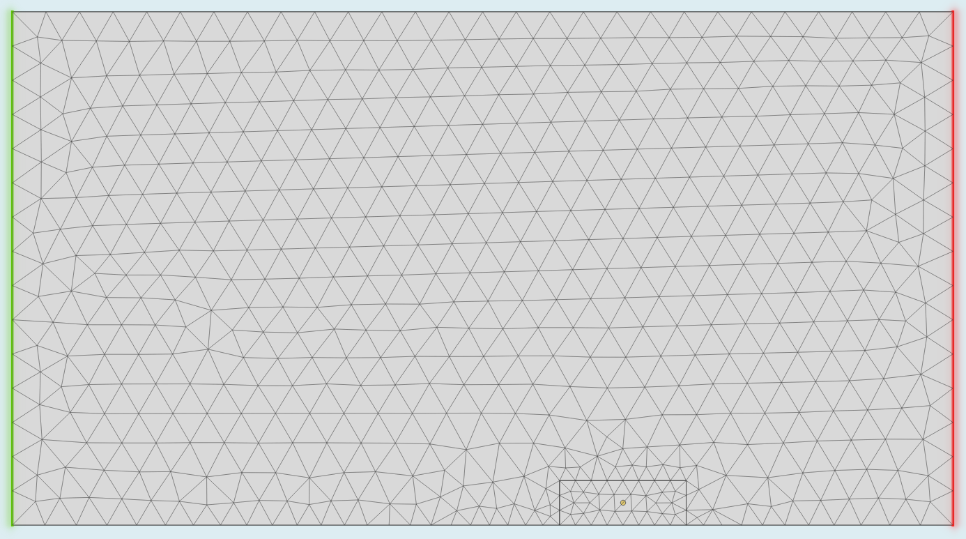
The mesh generation is based on the information of ‘Ground’ layer, particularly on its geometry and the ‘cellsize’ field. As we defined previously, the platform has a 0.2 m of element side length while the grate inlet area of 0.1 m. Go to Mesh manager (![]() ) and create a new one. As the platform is fully horizontal, keep all values by default and press OK (Fig. 5a). If we do so, the mesh generation process will succesfully finish (Fig. 5b) and the computational surface domain will be discretized as shonw in Fig. 5c.
) and create a new one. As the platform is fully horizontal, keep all values by default and press OK (Fig. 5a). If we do so, the mesh generation process will succesfully finish (Fig. 5b) and the computational surface domain will be discretized as shonw in Fig. 5c.
Once the mesh is generated, the current boundary conditions have been automatically assigned to this mesh. However, the user has the posibility to use any of the boundary conditions scenarios defined in the Boundary condition manager.
|
|
|
| (a) | (b) | (c) |
Fig. 5. Mesh generation: (a) definition of the mesh properties; (b) example of error message during the mesh generation; (c) view of the calculation mesh.
3.1.5 Run configuration
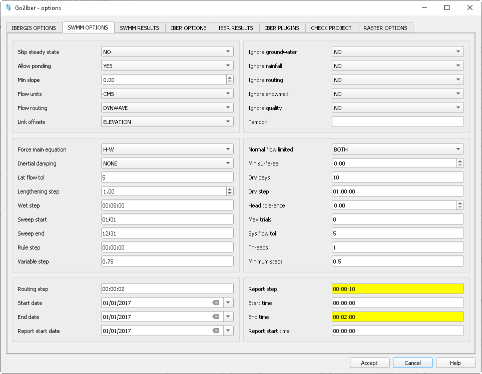
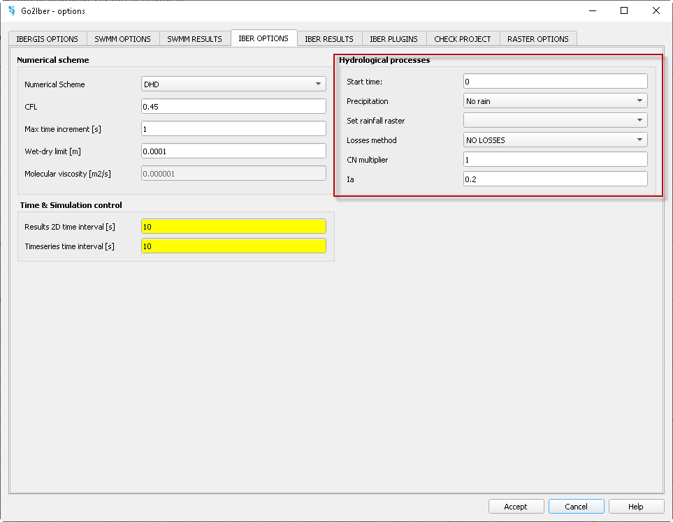
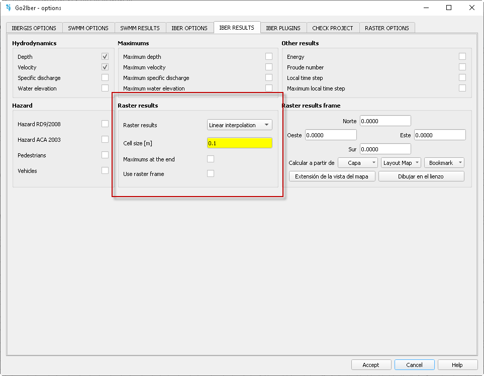
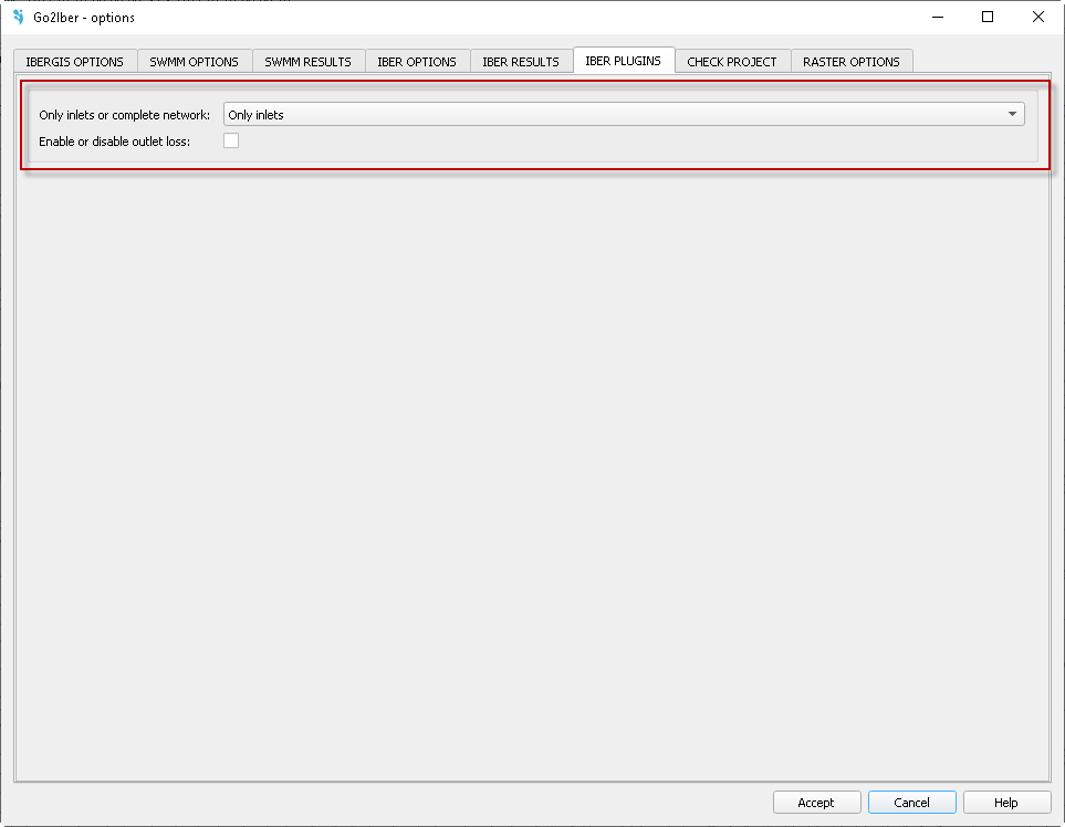
Finally, go to ‘Options’ button (![]() ) and configure the time parameters, results visualization and kind of simulation. In SWMM OPTIONS tab we have to define the ‘End time’ of 00:02:00 for the whole simulation, even if SWMM project is not defined (Fig. 6a). In such cases, Iber will take ‘End time’ as maximum simulation time. Also define a ‘Report step’ of 00:00:10. In tab IBER OPTIONS we have to define both writing times equal to 10 s, and the Hydrological process as No Rain and NO LOSSES (Fig. 6b). The results configuration (IBER RESULTS) by default except for Raster results options that must be defined with a ‘Cell size [m]’ of 0.1 and a Linear interpolation (Fig. 6c). Finally, as we do not have a SWMM project, we will simulate the urban drainage model considering only the inlets; thus, in IBER PLUGINS we must impose Only gullies (Fig. 6d). Accept the configuration.
) and configure the time parameters, results visualization and kind of simulation. In SWMM OPTIONS tab we have to define the ‘End time’ of 00:02:00 for the whole simulation, even if SWMM project is not defined (Fig. 6a). In such cases, Iber will take ‘End time’ as maximum simulation time. Also define a ‘Report step’ of 00:00:10. In tab IBER OPTIONS we have to define both writing times equal to 10 s, and the Hydrological process as No Rain and NO LOSSES (Fig. 6b). The results configuration (IBER RESULTS) by default except for Raster results options that must be defined with a ‘Cell size [m]’ of 0.1 and a Linear interpolation (Fig. 6c). Finally, as we do not have a SWMM project, we will simulate the urban drainage model considering only the inlets; thus, in IBER PLUGINS we must impose Only gullies (Fig. 6d). Accept the configuration.
|
|
| (a) | (b) |
|
|
| (c) | (d) |
Fig. 6. Run configuration: (a) definition of maximum simulation time (SWMM options); (b) Iber options definition; (c) Iber results definition; (d) Iber plugins definition.
To run the simulation, just click on ‘Execute model’ button (![]() ), select the mesh (Mesh1) and the folder where the model will be run. After checking all data, the Iber-SWMM simulation starts. Once the simulation finishes, the plugin asks for loading the results.
), select the mesh (Mesh1) and the folder where the model will be run. After checking all data, the Iber-SWMM simulation starts. Once the simulation finishes, the plugin asks for loading the results.
3.1.6 Results visualization
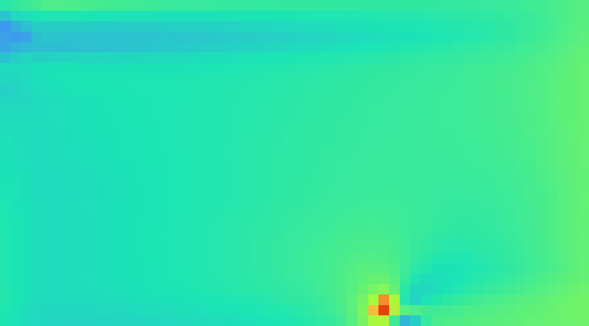
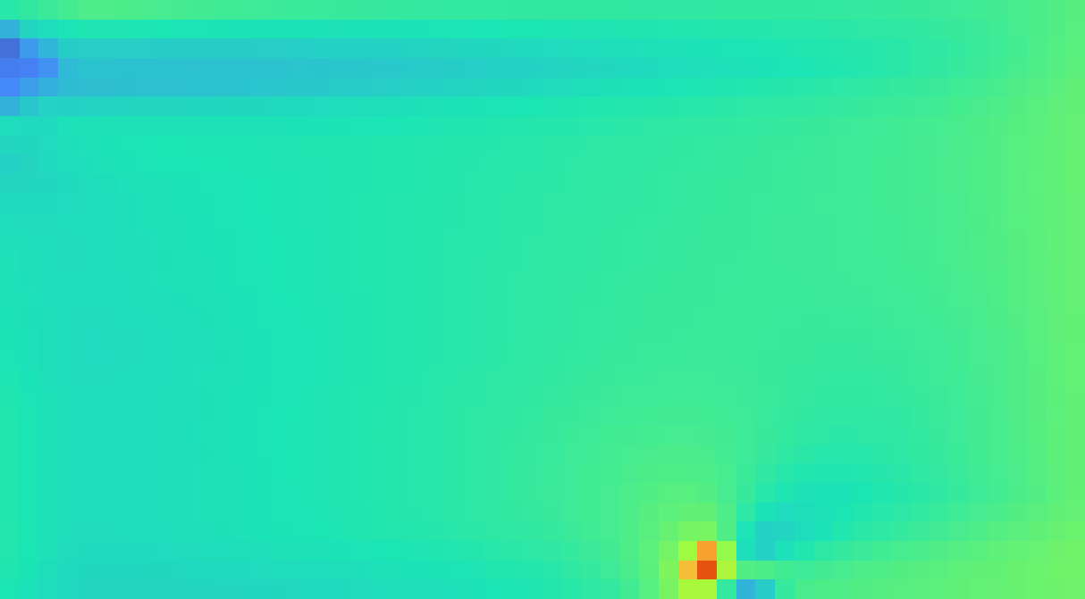
The results of the numerical models, SWMM and Iber, can be shown directly in QGIS. In this case, only the 2D results of Iber are available since none sewer network has been simulated through SWMM. Fig. 7 shows the map of flow depth and velocity at the end of the simulation. As expected, the inlet subtracts water from the model surface, affecting the hydrodynamics near the inlet location. The flow accelerates when it approaches to the inlet (Fig. 7b), especially in the X direction (Fig. 7c) while the velocity in the Y direction is almost null except near the inlet.

|

|
|

|
| (a) | (b) |
|

|

|

|
| (c) | (d) |
Fig. 7. Results at the end of the simulation: (a) flow depth; (b) flow velocity (modulus); (c) flow velocity in the X direction; (d) flow velocity in the Y direction.
3.2 Laboratory case: 'El Barrio'
This exercise will numerically replicate the Scientific Platform for Urban Runoff Testing located at the Center for Technological Innovation in Building and Civil Engineering (CITEEC) of the University of A Coruña. The experimental platform represents a perpendicular intersection of two streets and has a flat area of approximately 100 m2. The surface is connected to a drainage network consisting of four manholes, four pipes, one outlet point, and four inlets. It also has four ceramic tile roofs with variable slopes. Further information can be found in [1,18-20].
3.2.1 Data
The model will be build-up using the tools developed ad-hoc to facilitate the whole process. To that end, the following geometric entities are provided:
- GROUND_layer (shapefile)
- ROOF_layer (shapefile)
- INLETS_layer (shapefile)
- SWMM (*.ini and *inp)
- DEM (raster)
- Rainfall (text)
Each shapefile contains the database (*.dbf) with all data needed to compile the ‘Ground, ‘Roof’ and ‘Inlet’ layers. The SWMM model is also prepared and contains the sewer network information. The digital elevation model (DEM) is a raster file with ~4.4 cm pixel-size resolution, and represents the topography of the laboratory facility.
3.2.2 Model build-up
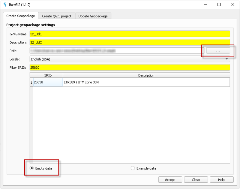
Once opened QGIS, load the IberGIS plugin by clicking on the icon ![]() , and the model generation window will appear (Fig. 8). Please, enter the name of the model (GPKG Name) and a description. Then, define the location and the coordinate system using the Spatial Reference System Identifier (SRID), in this case 25830.
, and the model generation window will appear (Fig. 8). Please, enter the name of the model (GPKG Name) and a description. Then, define the location and the coordinate system using the Spatial Reference System Identifier (SRID), in this case 25830.
|
Fig. 8. Model generation window. Create a new model or use the Example data model.
After a few seconds, the geopackage is generated with all features to build-up the model. First, we are going to import the SWMM model using the button “Import INP” (![]() ). The importation process of the SWMM model is automatic, and no user interaction is required.
). The importation process of the SWMM model is automatic, and no user interaction is required.
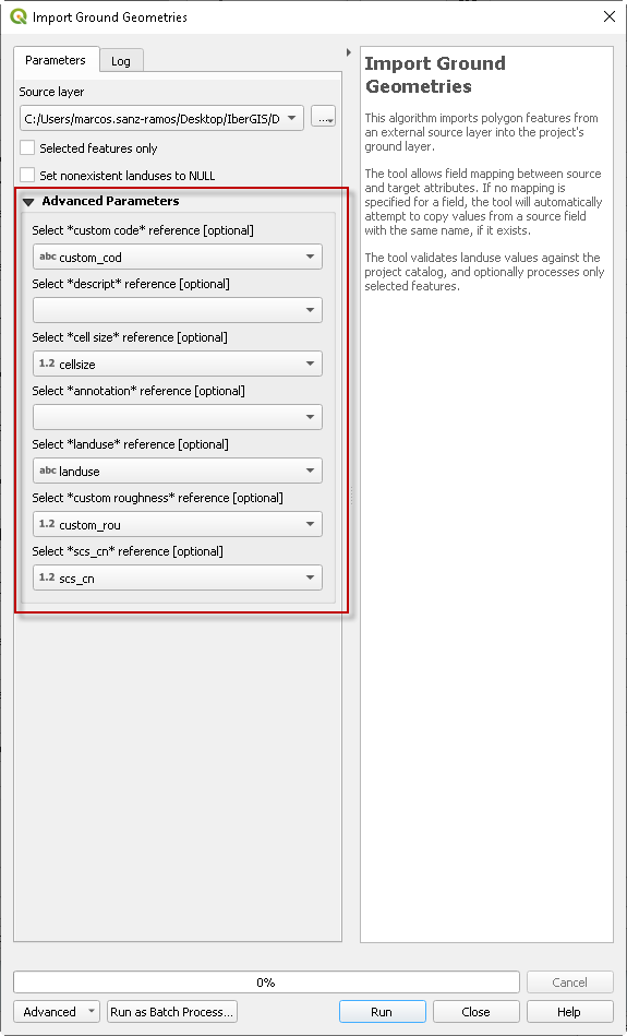
Then, we are going to import the ‘Ground’, ‘Roof’ and ‘Inlet’ layers through the “IberGIS” tools of the Processing Toolbox. In contrast with the SWMM file, to load the file of the geometric entities that define the two-dimensional computational domain, the user might select some fields to be imported to particular fields of the target file. To import the ‘Ground’ layer, go to Processing Toolbox >> IberGIS > Import Ground Geometries, select ‘GROUND_layer’ and define the correspondence of the original to the target database (Fig. 9a). To facilitate this process, similar field names are used in the original file.
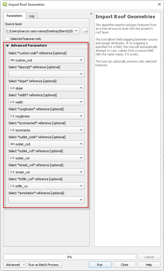
Continue with the ‘ROOF_layer’ through Processing Toolbox >> IberGIS > Import Roof Geometries, and define the correspondence of the original to the target database (Fig. 9b). It is important to highlight that if the field ‘outlet_code’ is used it must be properly defined according to the ‘custom_code’ of the ‘Junction’ layer of SWMM.
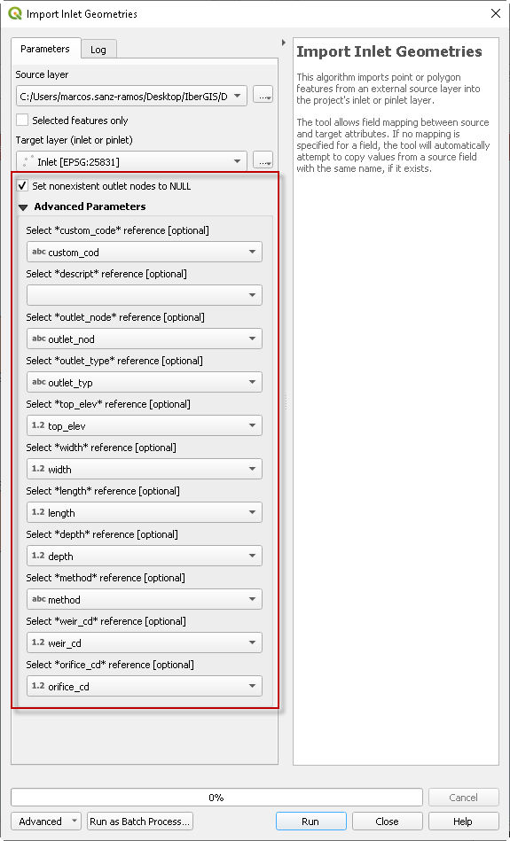
Finally, we import the ‘INLET_layer’ using the menu Processing Toolbox >> IberGIS > Import Inlet Geometries (Fig. 9c). It is worth noticing the target layer must be the one called ‘Inlet’ stored in the group ‘IBER’. Here we have to define properly the fields correspondence (similar field names are used in the original file).
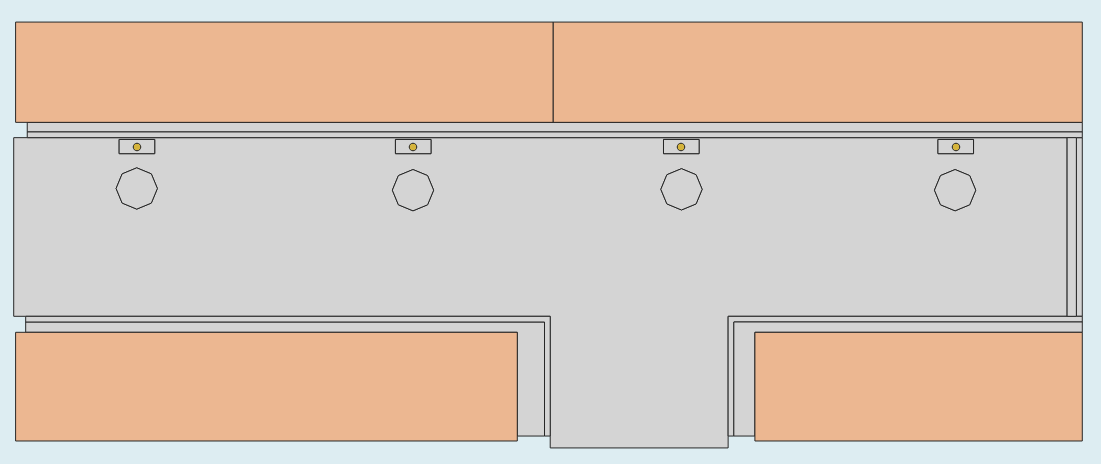
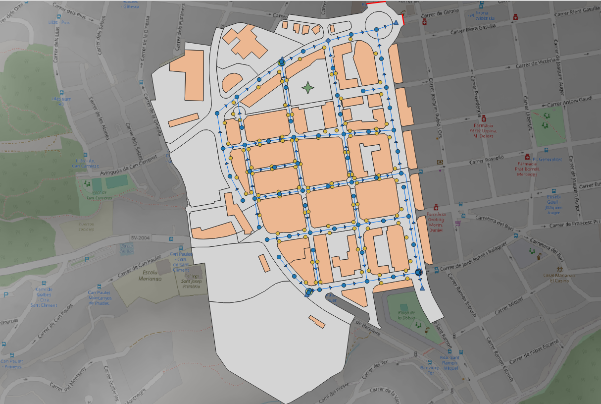
The result of these importation process is show in Fig. 9d. The computational domain is defined by a ground layer (grey polygon), a roof layer (ochre polygon), a inlets layer (yellow points), and the sewer network defined by junctions (blue points), conduits (blue lines) and an outfall (blue triangle).
|
|
|
| (a) | (b) | (c) |
|
| (d) |
Fig. 9. Generating the model domain. (a) Import ‘Ground’ layer window. (b) Import ‘Roof’ layer window. (c) Import ‘Inlet’ layer window. (d) Model domain after the importation process.
3.2.3 Hydraulic and hydrological conditions
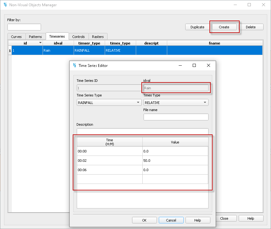
In this facility, the water enters from a rainfall simulator [18–20]. So, we have to define a hyetograph as a time series using the Non visual objects manager button ![]() . Here, we have first to create a Timeseries and, then, introduce the hyetograph provided in the models data (Rainfall.txt). Fig. 10a shows how to create the Timeseries and the configuration to define the hyetograph. Notice a hyetograph is defined as a constant rainfall (in mm/h) from the time when the rainfall value is first defined to the next time; thus, the last row is set as 0 mm/h to force the rain to stop. Otherwise, a constant rainfall intensity will be considered till the end of the simulation. Once the timeseries is defined, we have to create the ‘Hyetograph’ using the common tools of QGIS: select the ‘Hyetograph’ layer, enable the edition (
. Here, we have first to create a Timeseries and, then, introduce the hyetograph provided in the models data (Rainfall.txt). Fig. 10a shows how to create the Timeseries and the configuration to define the hyetograph. Notice a hyetograph is defined as a constant rainfall (in mm/h) from the time when the rainfall value is first defined to the next time; thus, the last row is set as 0 mm/h to force the rain to stop. Otherwise, a constant rainfall intensity will be considered till the end of the simulation. Once the timeseries is defined, we have to create the ‘Hyetograph’ using the common tools of QGIS: select the ‘Hyetograph’ layer, enable the edition (![]() ), and create a new one (
), and create a new one (![]() ) by clicking in the workspace. Immediately it will appear the attribute table creation window where we have only to select the timeseries (called “Rain”). A star-shaped icon (
) by clicking in the workspace. Immediately it will appear the attribute table creation window where we have only to select the timeseries (called “Rain”). A star-shaped icon (![]() ) will appear indicating there is a hyetograph defined. Notice, if a unique hyetograph is defined in the model, Iber assumes uniform rainfall over the whole computational domain; whereas, if more the one hyetographs are defined, Iber uses the Thiessen polygons method [1,22] to distribute spatially the rainfall according to each hyetograph.
) will appear indicating there is a hyetograph defined. Notice, if a unique hyetograph is defined in the model, Iber assumes uniform rainfall over the whole computational domain; whereas, if more the one hyetographs are defined, Iber uses the Thiessen polygons method [1,22] to distribute spatially the rainfall according to each hyetograph.
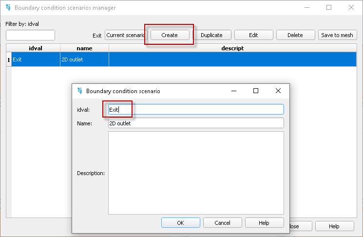
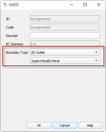
The unique boundary condition needed is an outlet located at the east of the model. To implement it, go to Boundary conditions manager (![]() ), create a new (Fig. 10b) one and assign as ‘Current scenario’. The manager window allows to store different inlet and outlet boundary conditions per scenario using the same ‘idval’ code. The definition of the outlet condition is carried out through the button Create boundary condition (
), create a new (Fig. 10b) one and assign as ‘Current scenario’. The manager window allows to store different inlet and outlet boundary conditions per scenario using the same ‘idval’ code. The definition of the outlet condition is carried out through the button Create boundary condition (![]() ). There we have to 1) select the line or lines that define de boundary conditions and 2) select the ‘Boundary type’ as “2D Outlet” with a “Supercritical/Critical” regime (Fig. 10c). This condition is saved in the layer ‘Boundary conditions’, which is stored in the group called ‘IBER’. It is important to highlight that any boundary condition must be implemented over a line of ‘Ground’ layer that belongs to a real boundary of the model. Hence, lines in contact with ‘Roof’ layer or inner lines must not be added as boundary condition. Abnormal results will appear in such case.
). There we have to 1) select the line or lines that define de boundary conditions and 2) select the ‘Boundary type’ as “2D Outlet” with a “Supercritical/Critical” regime (Fig. 10c). This condition is saved in the layer ‘Boundary conditions’, which is stored in the group called ‘IBER’. It is important to highlight that any boundary condition must be implemented over a line of ‘Ground’ layer that belongs to a real boundary of the model. Hence, lines in contact with ‘Roof’ layer or inner lines must not be added as boundary condition. Abnormal results will appear in such case.
|
|
|
| (a) | (b) | (c) |
Fig. 10. (a) Definition of a hyetograph as a timeseries. (b) Definition of a boundary condition. (c) Boundary condition creation window.
3.2.4 Mesh generation
The meshing process must be always done in the latest step, once all model conditions are implemented. This case requires the utilisation of a digital elevation model (DEM), that we have to load using the common tools of QGIS (Layer >> Add Layer >> Add Raster Layer). We recommend to add the file surface_DEM.tiff into ‘BASE MAP’ group.
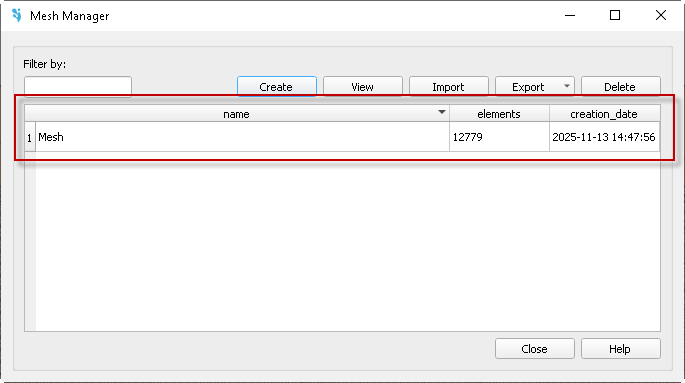
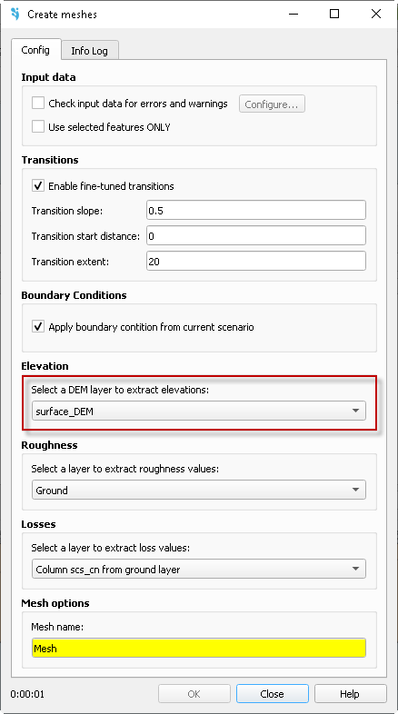
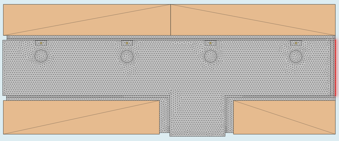
The mesh creation is carried out through the Mesh manager button (![]() ). There, the user can store different mesh configurations according to the mesh size defined in the field ‘cellsize’ of the ‘Ground’ layer, in combination with different boundary condition scenarios (Fig. 11a). In this case, the ‘cellsize’ is already defined as 0.1 m in ‘Ground’ layer; so, we have only to create it selecting the ‘surface_DEM’ raster layer in the Elevation section (Fig. 11b). We have also introduce a mesh name (“Mesh”), without spaces. The rest of parameters, by default (uncheck all Input data if it is checked). Press ‘Ok’ and the mesh will be generated (Fig. 11c) showing, besides the elements view for ‘Ground’ and ‘Roof’ layers, some information about the properties of the mesh (area and wrong normal).
). There, the user can store different mesh configurations according to the mesh size defined in the field ‘cellsize’ of the ‘Ground’ layer, in combination with different boundary condition scenarios (Fig. 11a). In this case, the ‘cellsize’ is already defined as 0.1 m in ‘Ground’ layer; so, we have only to create it selecting the ‘surface_DEM’ raster layer in the Elevation section (Fig. 11b). We have also introduce a mesh name (“Mesh”), without spaces. The rest of parameters, by default (uncheck all Input data if it is checked). Press ‘Ok’ and the mesh will be generated (Fig. 11c) showing, besides the elements view for ‘Ground’ and ‘Roof’ layers, some information about the properties of the mesh (area and wrong normal).
Finally, we have to assign the boundary condition scenario to this mesh. To do so, we have to open again the Boundary conditions manager, select the scenario and ‘Save to mesh’ selecting Mesh1.
|
|
| (a) | (b) |
|
| (c) |
Fig. 11. (a) Mesh properties. (b) Mesh manager window. (c) View of the computational mesh.
3.2.5 Run configuration
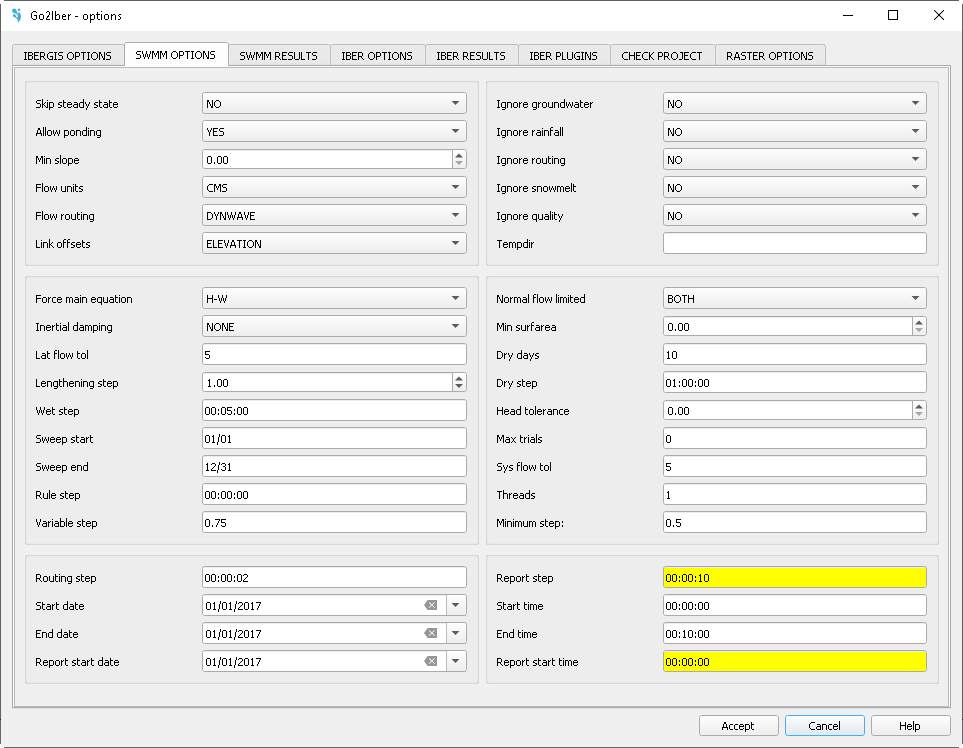
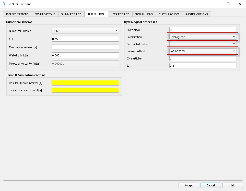
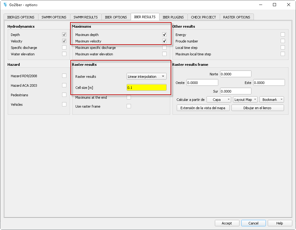
The model is almost ready to be simulated. Go to ‘Options’ button (![]() ) and configure the time parameters and results visualization. In SWMM OPTIONS tab (Fig. 12a) define the Report step (10 s) and End time (10 min). These values are mandatory and controls the maximum simulation time and the reporting results of SWMM. In IBER OPTIONS tab (Fig. 12b) we have to define the Results 2D time interval (10 s, the value as per SWMM results report) and the Timeseries time interval (10 s, not mandatory). Additionally, we have to activate the Hydrological process module of Iber by enabling Precipitation process (select ‘Hyetograph’ as rainfall type) and, in this case, disable Losses method (‘NO LOSSES’) as the laboratory facility is impervious. The rest of parameters, by default. Finally, in IBER RESULTS tab we have to enable Raster results as ‘Linear interpolation’ with a raster cell size of 0.1 m. Keep the rest of parameters by default and Accept the changes.
) and configure the time parameters and results visualization. In SWMM OPTIONS tab (Fig. 12a) define the Report step (10 s) and End time (10 min). These values are mandatory and controls the maximum simulation time and the reporting results of SWMM. In IBER OPTIONS tab (Fig. 12b) we have to define the Results 2D time interval (10 s, the value as per SWMM results report) and the Timeseries time interval (10 s, not mandatory). Additionally, we have to activate the Hydrological process module of Iber by enabling Precipitation process (select ‘Hyetograph’ as rainfall type) and, in this case, disable Losses method (‘NO LOSSES’) as the laboratory facility is impervious. The rest of parameters, by default. Finally, in IBER RESULTS tab we have to enable Raster results as ‘Linear interpolation’ with a raster cell size of 0.1 m. Keep the rest of parameters by default and Accept the changes.
|
|
|
| (a) | (b) | (c) |
Fig. 12. Go2Iber options windows: (a) SWMM options definition. (b) Iber options definition. (c) Iber results definition.
To run the simulation, just click on ‘Execute model’ button (![]() ), select the mesh (Mesh1) and the folder where the model will be run. After checking all data, the Iber-SWMM simulation starts. Once the simulation finish, the plugin asks for loading the results.
), select the mesh (Mesh1) and the folder where the model will be run. After checking all data, the Iber-SWMM simulation starts. Once the simulation finish, the plugin asks for loading the results.
3.2.6 Results visualization
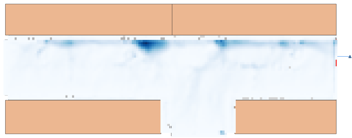
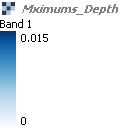
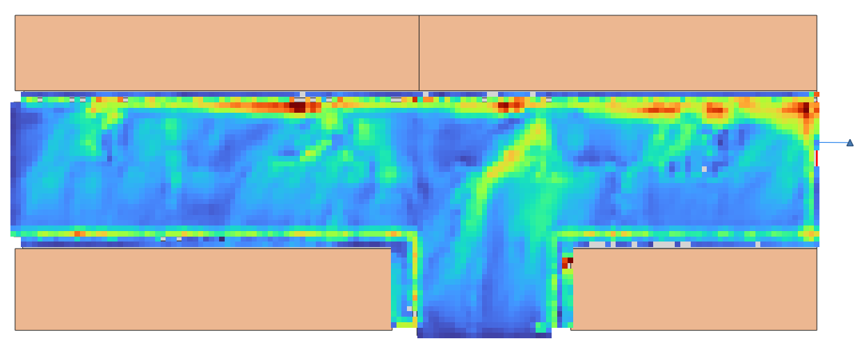
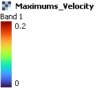
The results of the two numerical models, SWMM and Iber, can be shown directly in QGIS. First, the surface results are loaded automatically when the simulation ends. Fig. 13 shows the maximums values of the flow depth and velocity at the end of the simulation. We can observe how the topography plays an important role in the rainfall-runoff and flow propagation hydrodynamics; in this case, the flow tends to accumulate on the norther part of the main street as it commonly occurs in the cities due to the transversal slope of the streets. Major velocities are observed near the inlets, as we observed in the previous case.
|
|
| (a) |
|
|
| (b) |
Fig. 13. Results of maximums at the end of the simulation: (a) flow depth; (b) flow velocity (modulus).
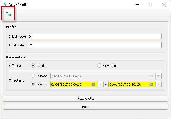
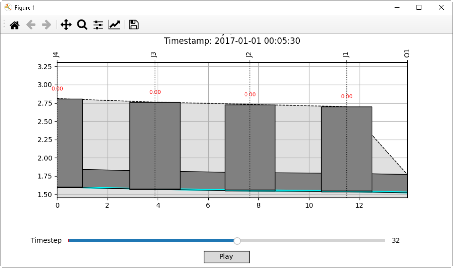
The results of SWMM can be loaded, as well as the Iber ones, by the button ‘Results’ (![]() ). Particularly, we are going to generate a profile along the sewer network conduits. To do so, a new window appear to select the nodes, the kind of offset (by depth or elevation) and the time limits (Fig. 14a). Choose the nodes (
). Particularly, we are going to generate a profile along the sewer network conduits. To do so, a new window appear to select the nodes, the kind of offset (by depth or elevation) and the time limits (Fig. 14a). Choose the nodes (![]() ), the offset by Depth and the time limits as shown in Fig. 14a. Then, once ‘Draw profile’ button is pressed, the profile will appear allowing some editing and the exportation of the figure (Fig. 14b). Additionally, this figure is dynamic and the profile can evolve along the time.
), the offset by Depth and the time limits as shown in Fig. 14a. Then, once ‘Draw profile’ button is pressed, the profile will appear allowing some editing and the exportation of the figure (Fig. 14b). Additionally, this figure is dynamic and the profile can evolve along the time.
|
|
| (a) | (b) |
Fig. 14. Profile results: (a) configuration windows; (b) profile from J4 to J1 node at 00:05:10.
3.3 Real case: synthetic rainfall
The last case aims of showing the performance of IberGIS at neighbourhood scale. It represents a particular zone of Sant Boi de Llobregat, a small town near Barcelona city (Spain). It has an area of ~32.5 ha and a sewer network composed by 66 junctions, 74 conduits and 4 outlets. The connection between the surface and subsurface systems is done by 103 inlets. The sewer network, inlets and roof properties, as well as the hydrological data, have been adapted looking for academic purposes.
3.3.1 Data
This case is provided in IberGIS as Example data. Thus, all data is provided within the geopackage of the Example data.
3.3.2 Model build-up
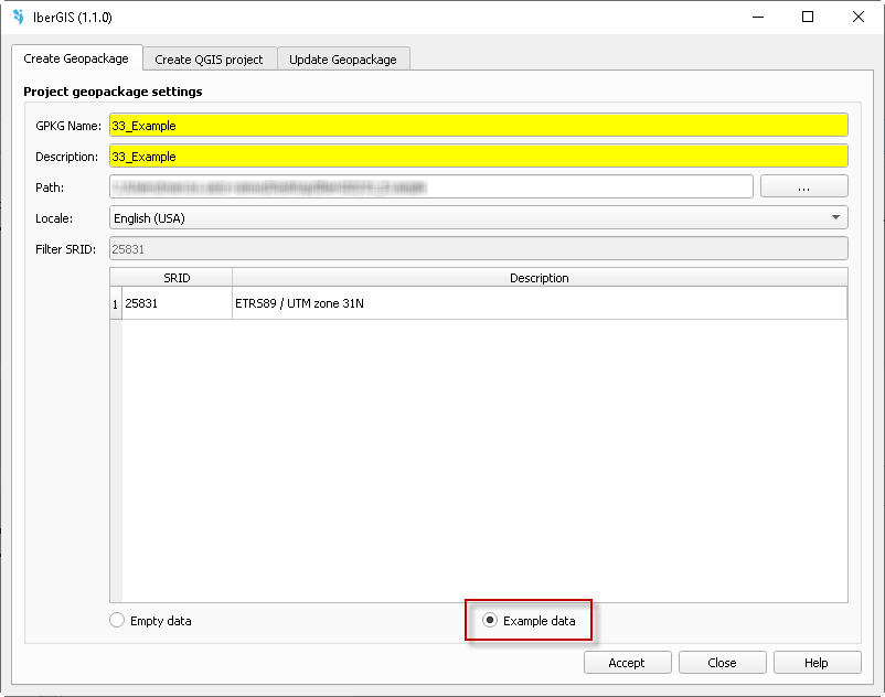
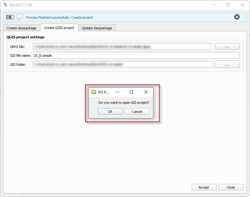
Open QGIS and load the IberGIS plugin by clicking on the icon ![]() . The model generation window will appear (Fig. 15). Please, select Example data and enter the model name (GPKG Name) and a description. The location and the coordinate system using the Spatial Reference System Identifier (SRID) is defined automatically (25831, Catalonia, Spain).
. The model generation window will appear (Fig. 15). Please, select Example data and enter the model name (GPKG Name) and a description. The location and the coordinate system using the Spatial Reference System Identifier (SRID) is defined automatically (25831, Catalonia, Spain).
|
|
| (a) | (b) |
|
| (c) |
Fig. 15. Model generation window: (a) use the Example data model; (b) load the geopackage. (c) General view of the study area.
The unique data provided is the digital terrain model (DTM) of the study area generated by the Cartographic and Geologic Institute of Catalonia [23], a 2 m-size raster file that covers the entire computational domain. We can load it anywhere (![]() ), but we recommend to use the BASE MAP layer, below the layer OSM Standard (Fig. 15c).
), but we recommend to use the BASE MAP layer, below the layer OSM Standard (Fig. 15c).
3.3.3 Hydraulic and hydrological conditions
Despite the model is ready to run, we are going to check all data, conditions and options. The model is already defined and the essential data of SWMM, IBER and MESH layers are included. If we open the attribute table of ‘Ground’ layer, we can observe that the cellsize is set to 10 m. Since the DTM has a resolution of 2 m, we can use this cellsize value instead. So, enable editing (![]() ) and use the field calculator (
) and use the field calculator (![]() ) to update this parameter for the whole entities of this layer. We also modify the ‘scs_cn’ parameter to 90 (Fig. 16a).
) to update this parameter for the whole entities of this layer. We also modify the ‘scs_cn’ parameter to 90 (Fig. 16a).
It is worth noticing that in ‘Ground’ layer there are two related fields: ‘landuse’ and ‘custom_roughness’ (Fig. 16a). If a real value is defined in ‘custom_roughness’, it will be used as Manning coefficient instead of the values defined in the layer ‘Landuses’ of the IBER group. We can also use a raster of Manning coefficient values if the user select it during the mesh generation process.
The ‘Roof’ layer shows relevant information about the roof properties (Fig. 16b), such as the slope, width, roughness, percentage of spilled volume to street, sewer or infiltrates, and what kind of connection have (isconnected: 1, 100% connected; 2, partially connected; 3, disconnected). Keep this layer by default.
The ‘Inlet’ layer also contains all the information of the inlets (Fig. 16c). It is worth noticing that the ‘outlet_type’ is set as TO NETWORK for all inlets because we are going to simulate the complete network. Also, ‘outlet_node’ is set using the same name as the ‘code’ field of the ‘Junction’ layer (Fig. 16d). As we can observe, more than one inlet can be connected to a one junction. Keep these layers by default.

|
| (a) |

|
| (b) |

|
| (c) |

|
| (d) |
Fig. 16. Attribute tables: (a) ‘Ground’ layer; (b) ‘Roof’ layer; (c) ‘Inlet’ layer; (d) ‘Junction’ layer.
Keep the rest of layers by default, although we encourage to have a look on it. For example, if we open the ‘Hyetograph’ layer (![]() , we can check that there is a ‘timeseries’ called T5-5m selected. Check in Non visual object manager (
, we can check that there is a ‘timeseries’ called T5-5m selected. Check in Non visual object manager (![]() ) the values of this hyetograph, with a maximum rainfall intensity of 8.75 mm/h. Modify this hyetograph by adding an extra row at the end (01:00) with none intensity (0 mm/h) to indicate that the rainfall event ends.
) the values of this hyetograph, with a maximum rainfall intensity of 8.75 mm/h. Modify this hyetograph by adding an extra row at the end (01:00) with none intensity (0 mm/h) to indicate that the rainfall event ends.
We can also check the kind of ‘Boundary conditions’ showing the attribute table of this layer: two outlet conditions have been assigned to two lines located at north (Fig. 15c). We can edit or add more editing this layer by using the button Create boundary condition (![]() ).
).
3.3.4 Mesh generation
We are going to generate a mesh (e.g., called Mesh1) using the default values of the Mesh manager button (![]() ). We have to select the DTM raster as the elevation file for the 'Ground' layer. The rest of parameters by default.
). We have to select the DTM raster as the elevation file for the 'Ground' layer. The rest of parameters by default.
3.3.5 Run configuration
The model is ready to be simulated, so we can run the simulation immediately. However, we have to check the ‘Options’ (![]() ) and see what configuration will be used. In SWMM OPTIONS tab the Report step is set as 5 min and the End time at 3 h. In IBER OPTIONS tab we have to define the Precipitation as Hyetograph and Losses method as SCS. Finally, in IBER RESULTS tab we have to enable Raster results as ‘Linear interpolation’ with a raster cell size of 2 m. We are going to simulate the Complete network (IBER PLUGINS) and define a maximum value for depth and velocity legend of 0.25 m and 0.5 m/s (IBERGIS OPTIONS). If the limits are not defined, IberGIS will autimatically defined it each time step.
) and see what configuration will be used. In SWMM OPTIONS tab the Report step is set as 5 min and the End time at 3 h. In IBER OPTIONS tab we have to define the Precipitation as Hyetograph and Losses method as SCS. Finally, in IBER RESULTS tab we have to enable Raster results as ‘Linear interpolation’ with a raster cell size of 2 m. We are going to simulate the Complete network (IBER PLUGINS) and define a maximum value for depth and velocity legend of 0.25 m and 0.5 m/s (IBERGIS OPTIONS). If the limits are not defined, IberGIS will autimatically defined it each time step.
To run the simulation, just click on ‘Execute model’ button (![]() ), select the mesh (Mesh1) and the folder where the model will be run. After checking all data, the Iber-SWMM simulation starts. Once the simulation finish, the plugin asks for loading the results.
), select the mesh (Mesh1) and the folder where the model will be run. After checking all data, the Iber-SWMM simulation starts. Once the simulation finish, the plugin asks for loading the results.
3.3.6 Run configuration
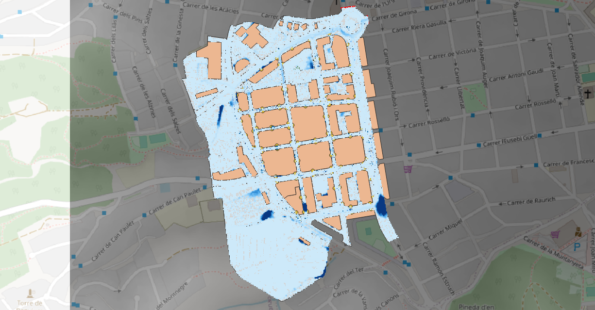
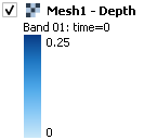
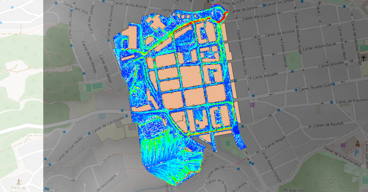
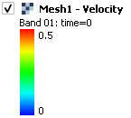
Once the simulation ends, accept loading the results of the simulation and, then, visualize them at 1 h of simulation. Fig. 17 shows the map of water depth and flow velocity (modulus) on the surface (results of Iber), and how the flow is transported over the streets mainly to the NE direction (where the outlet conditions are implemented). Considerable water accumulation is produced in five to nine locations (Fig. 18a) due to topographical depressions and the no consideration of outlet conditions (e.g., at southern part of the model).
|
|
| (a) |
|
|
| (b) |
Fig. 17. Hydrodynamic results on surface 1 h after the simulation starts: (a) depths; (b) velocities.
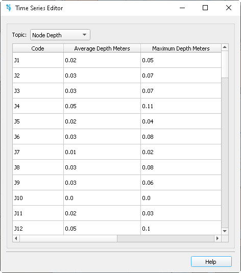
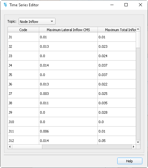
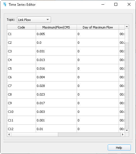
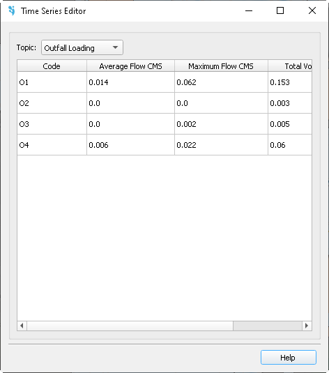
We can also check the Report summary of SWMM results. Fig. 18 shows an example for node depths, node inflows, link flows and outfall loading. Junction J60 presents a maximum depth of 3.55 m; thus, this node is under pressure and the flow goes from the sewer network to the street (this is one of the causes of water accumulation there, see Fig. 18a). In Node subcharge option we can observe that this node is working in pressurized flow for more than 2 hours.
The outfall that spills the maximum discharge is O1, located at NE, with a peak discharge above 0.06 m3/s. This is because the sewer network mainly drains into this direction, and the flow in the conduits tends to accumulate in such direction.
|
|
|
|
| (a) | (b) | (c) | (d) |
Fig. 18. Hydrodynamic results in the sewer network (Summary report): (a) node depths; (b) node inflow; (c) link flow; (d) outfall loading.
Funding
This publication is part of the project “DRAIN - Digital RAIN. An integrated model of urban drainage” (CPP2021-008756) funded by the Spanish Ministry of Science, Innovation and Universities - State Research Agency (MCIN/AEI/10.13039/501100011033) and by the European Union “Next Generation EU/PRTR”.
References
[1] E. Sañudo, L. Cea, J. Puertas, Modelling Pluvial Flooding in Urban Areas Coupling the Models Iber and SWMM, Water (Switzerland) 12 (2020) 2647. https://doi.org/https://doi.org/10.3390/w12092647.
[2] E. Sañudo, O. García-Feal, L. Hagen, L. Cea, J. Puertas, C. Montalvo, R. Alvarado-Vicencio, J. Hofmann, IberSWMM+: A high-performance computing solver for 2D-1D pluvial flood modelling in urban environments, J. Hydrol. 651 (2025) 132603. https://doi.org/10.1016/j.jhydrol.2024.132603.
[3] M. Sanz-Ramos, E. Sañudo, D. López-Gómez, O. García-Feal, E. Bladé, L. Cea, Evolución de la modelización numérica bidimensional del flujo en lámina libre a través del software Iber, Ing. Del Agua 29 (2025) 114–131. https://doi.org/10.4995/ia.2025.23259.
[4] M. Gómez, B. Russo, Hydraulic Efficiency of Continuous Transverse Grates for Paved Areas, J. Irrig. Drain. Eng. 135 (2009) 225–230. https://doi.org/10.1061/(ASCE)0733-9437(2009)135:2(225).
[5] M. Gómez, B. Russo, Comparative Study Of Methodologies To Determine Inlet Efficiency From Test Data: HEC-12 Methodology Vs UPC Method, Water Resour. Manag. III. WIT Trans. Ecol. Environ. 80 (2005) 623–632. https://doi.org/10.2495/WRM050621.
[6] M. Gómez, J. Parés, B. Russo, E. Martínez‐Gomariz, Methodology to quantify clogging coefficients for grated inlets. Application to SANT MARTI catchment (Barcelona), J. Flood Risk Manag. 12 (2019). https://doi.org/10.1111/jfr3.12479.
[7] M. Gómez, B. Russo, J. Tellez-Alvarez, Experimental investigation to estimate the discharge coefficient of a grate inlet under surcharge conditions, Urban Water J. 16 (2019) 85–91. https://doi.org/10.1080/1573062X.2019.1634107.
[8] M. Gómez, J. Tellez-Alvarez, B. Russo, Discharge coefficients to be used in inlet hydraulics, Proc. Inst. Civ. Eng. Water Manag. (2023) 1–11. https://doi.org/10.1680/jwama.22.00059.
[9] M. Sanz-Ramos, J. Téllez-Álvarez, E. Bladé, M. Gómez-Valentín, J.D. Tellez Alvarez, E. Bladé, M. Gómez-Valentín, Simulating the hydrodynamics of sewer-inlets using 2D-SWE based model, in: Adv. Hydroinformatics. SimHydro 2019 - Model. Extrem. Situations Cris. Manag., Springer Singapore, 2020: pp. 821–838. https://doi.org/10.1007/978-981-15-5436-0.
[10] J. Tellez-Alvarez, M. Gómez, B. Russo, Quantification of Energy Loss in Two Grated Inlets under Pressure, Water 12 (2020) 1601. https://doi.org/10.3390/w12061601.
[11] E. Martínez-Gomariz, M. Gómez, B. Russo, P. Sánchez, J.-A. Montes, Methodology for the damage assessment of vehicles exposed to flooding in urban areas, J. Flood Risk Manag. 12 (2018) e12475. https://doi.org/10.1111/jfr3.12475.
[12] E. Martínez-Gomariz, M. Gómez, B. Russo, S. Djordjević, A new experiments-based methodology to define the stability threshold for any vehicle exposed to flooding, Urban Water J. 14 (2017) 1–10. https://doi.org/10.1080/1573062X.2017.1301501.
[13] E. Martínez-Gomariz, M. Gómez, B. Russo, P. Sánchez, J.A. Montes, Metodología para la evaluación de daños a vehículos expuestos a inundaciones en zonas urbanas, Ing. Del Agua 21 (2017) 247. https://doi.org/10.4995/ia.2017.8772.
[14] E. Martínez‐Gomariz, B. Russo, M. Gómez, A. Plumed, An approach to the modelling of stability of waste containers during urban flooding, J. Flood Risk Manag. 13 (2020). https://doi.org/10.1111/jfr3.12558.
[15] B. Russo, D. Sunyer, M. Velasco, S. Djordjević, Analysis of extreme flooding events through a calibrated 1D/2D coupled model: the case of Barcelona (Spain), J. Hydroinformatics 17 (2015) 473–491. https://doi.org/10.2166/hydro.2014.063.
[16] M. Gómez, J. Recasens, B. Russo, E. Martínez-Gomariz, E. Martinez-Gomariz, Assessment of inlet efficiency through a 3D simulation: numerical and experimental comparison, Water Sci. Technol. 74 (2016) 1926–1935. https://doi.org/10.2166/wst.2016.326.
[17] J. Tellez, M. Gómez, B. Russo, J.M. Redondo, Characterize the hydraulic behaviour of grate inlet in urban drainage to prevent the urban’s flooding, in: EGU Gen. Assem. 2016, Viena (Austria), 2016. https://doi.org/10.1061/(ASCE)IR.1943-4774.0000625.
[18] E. Sañudo, L. Cea, J. Puertas, J. Naves, J. Anta, Large‐scale physical facility and experimental dataset for the validation of urban drainage models, Hydrol. Process. 38 (2024). https://doi.org/10.1002/hyp.15068.
[19] J. Naves, J. Anta, J. Suárez, J. Puertas, Hydraulic, wash-off and sediment transport experiments in a full-scale urban drainage physical model, Sci. Data 7 (2020) 44. https://doi.org/10.1038/s41597-020-0384-z.
[20] E. Sañudo, L. Cea, J. Puertas, Comparison of three different numerical implementations to model rainfall‐runoff transformation on roofs, Hydrol. Process. 36 (2022). https://doi.org/10.1002/hyp.14588.
[21] J.L. Aragón Hernández, G.A. Aguilar Martínez, U. Velázquez Ríos, M.R. Jiménez Magaña, A. Maya Franco, Distribución espacial de variables hidrológicas. Implementación y evaluación de métodos de interpolación, Ing. Investig. y Tecnol. 20 (2019) 1–15. https://doi.org/10.22201/fi.25940732e.2019.20n2.023.
[22] V.T. Chow, D.R. Maidment, L.W. Mays, Applied Hydrology, MCGRAW-HIL, New York, USA, 1988..
[23] ICGC, Descàrregues, Inst. Cart. i Geològic Catalunya (2021). https://www.icgc.cat/Descarregues (accessed February 2, 2021).
Document information
Published on 27/10/25
DOI: 10.23967/iber.2025.03
Licence: CC BY-NC-SA license
Share this document
Keywords
claim authorship
Are you one of the authors of this document?